A NEW REAL- TIME FAULT DETECTION

METHODOLOGY FOR SYSTEMS UNDER TEST

PHASE I REPORT

SUBMITTED BY:

DR. ROGER W. JOHNSON, Ph.D., PE

ASSOCIATE PROFESSOR

MECHANICAL, MATERIALS ANDAEROSPACE ENGINEERING

UNIVERSITY OF CENTRAL FLORIDA

ORLANDO, FL 32816

SEPTEMBER 19 th, 1998

CONTRIBUTING GRADUATE STUDENTS:

SAN JAY JAYARAM

RICHARD A. HULL

https://ntrs.nasa.gov/search.jsp?R=20000028356 2018-07-14T20:44:40+00:00Z

F #

f

TABLE OF CONTENTS

1. SUMMARY ............................................................................................................ 1

2. FLIGHT CONTROL ............................................................................................. 2

2.1 Introduction .......................................................................................................... 2

2.2 Statement of Work ................................................................................................ 2

2.3 Objectives ............................................................................................................ 3

2.4 Approach .............................................................................................................. 4

42.5 Flight Control Example ........................................................................................

2.6 System Identification Using MATLAB .................................................................. 7

2.7 Error Detection Filter ........................................................................................... 13

2.8 Detection Filter Algorithm .................................................................................. 14

3. KALMAN FILTERING FOR SIGNAL CONDITIONING ....................... 17

3.1 Kalman Filter Formulations ................................................................................ 18

3.2 Study on Optimal Trajectories of Model State Variables ..................................... 21

3.3 Calculation of Optimal Equations ....................................................................... 21

4. SIMULATION RESULTS ................................................................................ 26

5. LIST OF REFERENCES .................................................................................. 30

(

APPENDIX A

Input - Output Data of Pitch Actuator Controller Test Sequence Used (Figure)

(

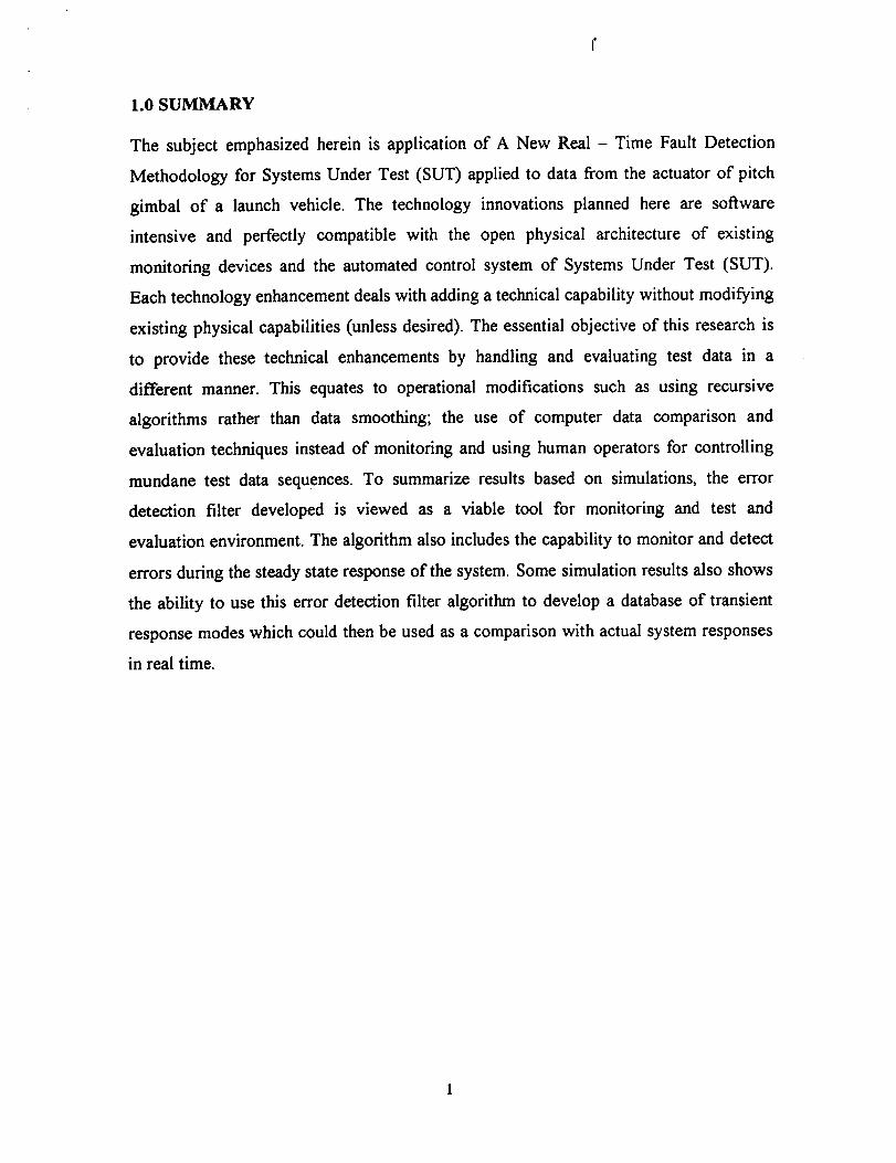
1.0 SUMMARY

The subject emphasized herein is application of A New Real - Time Fault Detection

Methodology for Systems Under Test (SUT) applied to data from the actuator of pitch

gimbal of a launch vehicle. The technology innovations planned here are sottware

intensive and perfectly compatible with the open physical architecture of existing

monitoring devices and the automated control system of Systems Under Test (SUT).

Each technology enhancement deals with adding a technical capability without modifying

existing physical capabilities (unless desired). The essential objective of this research is

to provide these technical enhancements by handling and evaluating test data in a

different manner. This equates to operational modifications such as using recursive

algorithms rather than data smoothing; the use of computer data comparison and

evaluation techniques instead of monitoring and using human operators for controlling

mundane test data sequences. To summarize results based on simulations, the error

detection filter developed is viewed as a viable tool for monitoring and test and

evaluation environment. The algorithm also includes the capability to monitor and detect

errors during the steady state response of the system. Some simulation results also shows

the ability to use this error detection filter algorithm to develop a database of transient

response modes which could then be used as a comparison with actual system responses

in real time.

f

2 - FLIGHT CONTROL

2.1 - INTRODUCTION

The complex automatic systems so widely employed in modern industry can consist of

hundreds of inter-dependent working parts, which are individually subject to malfunction

or failure. It is therefore necessary to provide the required operation of the entire system

by a scheme of monitoring which detects a fault as it occurs, thereby identifying the

malfunction of the faulty component. The principal concern here is this monitoring

function, i.e., the detection, prediction and identification of faults during on-line (real-

time) operation of a dynamic system.

2.2 STATEMENT OF WORK

Upon studying and analyzing the previous work done by various engineers on fault

detection systems, emphasis is given here on a simpler and more effective means of

automatic fault detection methodology which applies the basic principles of identifying

the system and using the model based simulations for detecting failures in the system

components. In the next section, the approach taken is discussed.

The purpose of this research is focussed on the identification/demonstration of critical

technology innovations that will be applied to various applications viz. Detection of

automated machine Health Monitoring (HM), real-time data analysis and control of

Systems Under Test (SUT). This new innovation using a High Fidelity Dynamic Model-

based Simulation (HFDMS) approach will be used to implement a real-time monitoring,

Test and Evaluation (T&E) methodology including the transient behavior of the system

under test. The unique element of this process control technique is the use of high

fidelity, computer generated dynamic models to replicate the behavior of actual Systems

Under Test (SUT). It will provide a dynamic simulation capability that becomes the

reference truth model, from which comparisons are made with the actual raw/conditioned

data from the test elements.

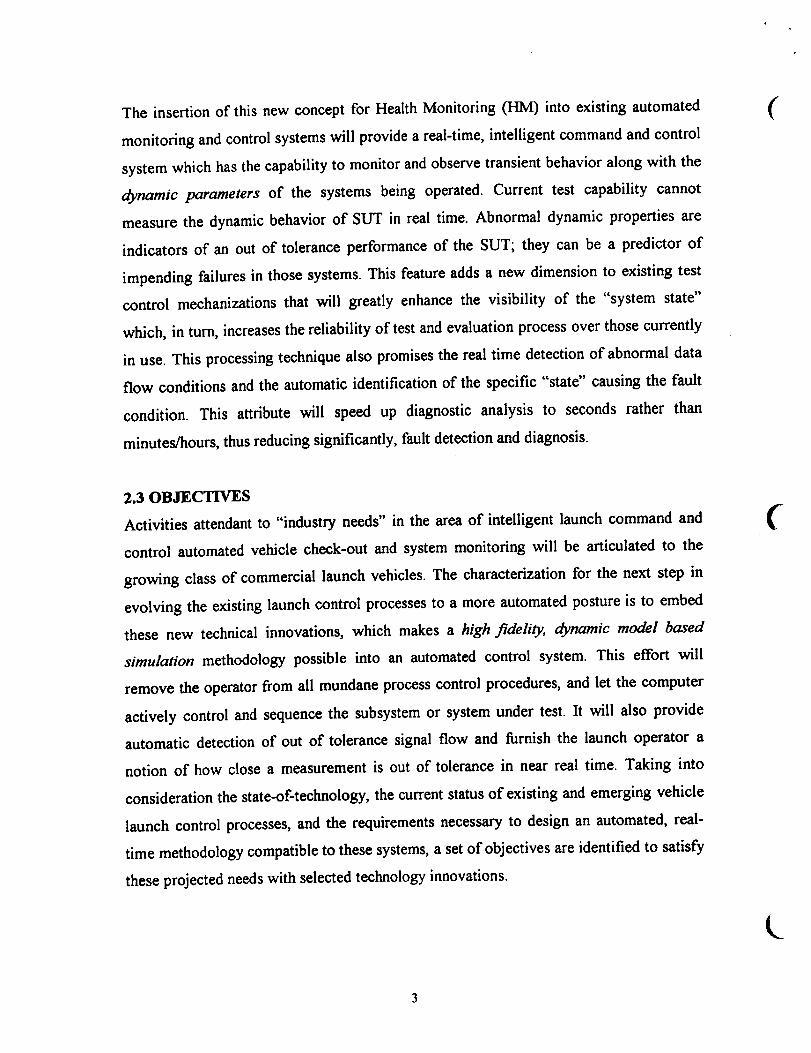
The insertionof this new concept for Health Monitoring (HM) into existing automated

monitoring and control systems will provide a real-time, intelligent command and control

system which has the capability to monitor and observe transient behavior along with the

dynamic parameters of the systems being operated. Current test capability cannot

measure the dynamic behavior of SUT in real time. Abnormal dynamic properties are

indicators of an out of tolerance performance of the SUT; they can be a predictor of

impending failures in those systems. This feature adds a new dimension to existing test

control mechanizations that will greatly enhance the visibility of the "system state"

which, in turn, increases the reliability of test and evaluation process over those currently

in use. This processing technique also promises the real time detection of abnormal data

flow conditions and the automatic identification of the specific "state" causing the fault

condition. This attribute will speed up diagnostic analysis to seconds rather than

minutes/hours, thus reducing significantly, fault detection and diagnosis.

(

2.30B,1ECTIVES

Activities attendant to "industry needs" in the area of intelligent launch command and

control automated vehicle check-out and system monitoring will be articulated to the

growing class of commercial launch vehicles. The characterization for the next step in

evolving the existing launch control processes to a more automated posture is to embed

these new technical innovations, which makes a high fidelity, dynamic model based

simulation methodology possible into an automated control system. This effort will

remove the operator from all mundane process control procedures, and let the computer

actively control and sequence the subsystem or system under test. It will also provide

automatic detection of out of tolerance signal flow and furnish the launch operator a

notion of how close a measurement is out of tolerance in near real time. Taking into

consideration the state-of-technology, the current status of existing and emerging vehicle

launch control processes, and the requirements necessary to design an automated, real-

time methodology compatible to these systems, a set of objectives are identified to satisfy

these projected needs with selected technology innovations.

_

The following objectives will describe the scope of this research:

1. Identifying the System that is under test and developing a High Fidelity Dynamic

Model using the input output data sequence of the actual system.

2. Formulate and apply a new innovation using a High Fidelity Dynamic Model based

Simulation approach to implement a real time monitoring system for automating a

detection system for detecting an "abnormal signal flow" in the Engine Flight Control

System (in particular, the actuator of the pitch axis).

3. Use a Kalman Filter estimation mechanization to reduce raw measurement error

before correlation between simulated and actual responses are generated.

2.4 APPROACH

The approach taken in the development of detection methodology for automating the

control system is to employ High Fidelity Dynamic Model Based Simulation (HFDMS)

method to conduct Test and Evaluation (T&E) procedures. This new innovation of using

Dynamic models (i.e. those that include the characteristic differential equations along

with their dynamic parameters) to replicate the behavior of the actual system under test,

results in a dynamic simulation capability that becomes the reference or truth model,

from which, comparisons are made with the actual raw data from test elements. If

detection of an "abnormal flow" is triggered, an automatic hand-over to the designated

diagnostic component model is implemented for resolution [Ref: 3 and 4].

2.5 FLIGHT CONTROL EXAMPLE

A real - time monitoring and error detection algorithm is developed for application with a

missile control system actuator. A second order discretized model of a first stage rocket

engine pitch gimbal actuator system is developed. An error detection algorithm and

filtering approach is then developed which compares the model output to in-coming data

in real-time. A recursive approximation to the mean square error (MSE) is obtained via a

discrete low pass filter and used with a dynamic threshold detection algorithm. A novel

feature of this method is the use of model rate information and a matched filter approach

to generate the dynamic error threshold. This enables good detection results to be

4

obtainedfor errors in both transient and steady state response characteristics. Actual pre-

launch data is then used to verify the performance of this error detection filter [Ref: 3].

(

ACTUATOR SUBSYSTEM MODEL:

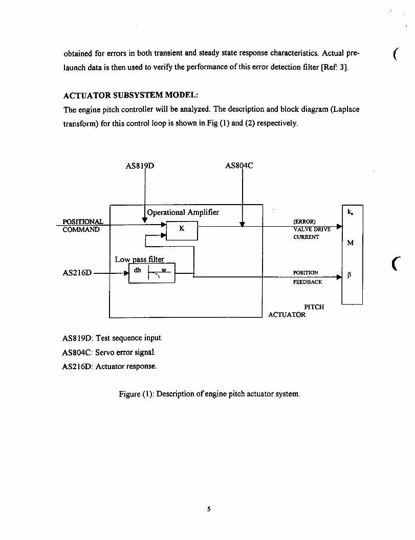
The engine pitch controller will be analyzed. The description and block diagram (Laplace

transform) for this control loop is shown in Fig (1) and (2) respectively.

POSITIONALCOMMAND

AS216D

AS8 )D AS804C

Operational Amplifier

SLow pass filter

r (ERROR)VALVE DRIVE _

CURRENT

POSITION

FEEDBACK

PITCH

ACTUATOR

AS819D: Test sequence input.

AS804C: Servo error signal.

AS216D: Actuator response.

Figure (1): Description of engine pitch actuator system.

5

R(s) E(s)

(GAIN)

w tSIU ACTUATOR

Y(s)

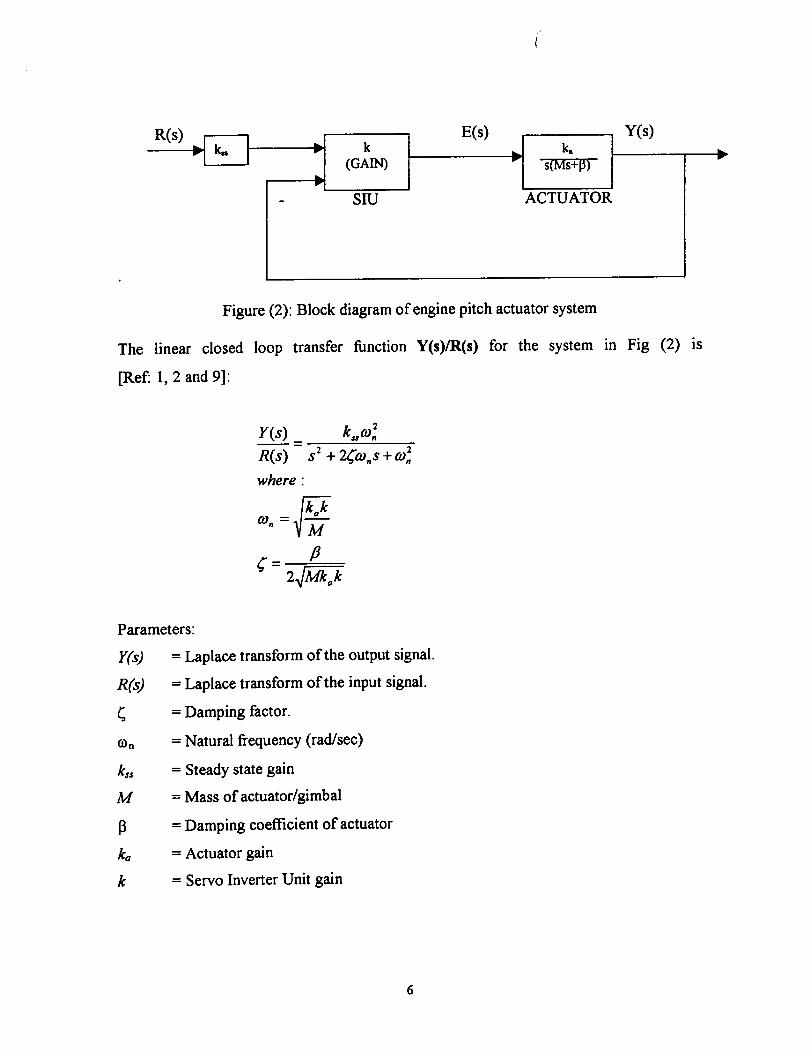
Figure (2): Block diagram of engine pitch actuator system

The linear closed loop transfer function Y(s)/R(s) for the system

[Ref: 1, 2 and 9]:

in Fig (2) is

m

n(s) s _+ z((o.s + co_.where:

P

Parameters:

r(s)

R(s)

On

M

ko

k

= Laplace transform of the output signal.

= Laplace transform of the input signal.

= Damping factor.

= Natural frequency (rad/sec)

= Steady state gain

= Mass of actuator/gimbal

= Damping coefficient of actuator

= Actuator gain

= Servo Inverter Unit gain

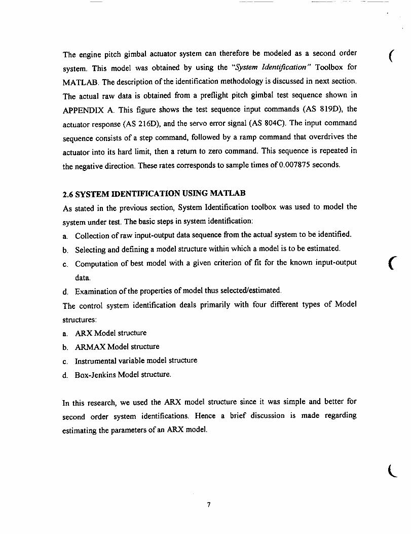
The engine pitch gimbal actuator system can therefore be modeled as a second order

system. This model was obtained by using the "System Identification" Toolbox for

MATLAB. The description of the identification methodology is discussed in next section.

The actual raw data is obtained from a preflight pitch gimbal test sequence shown in

APPENDIX A. This figure shows the test sequence input commands (AS 819D), the

actuator response (AS 216D), and the servo error signal (AS 804C). The input command

sequence consists of a step command, followed by a ramp command that overdrives the

actuator into its hard limit, then a return to zero command. This sequence is repeated in

the negative direction. These rates corresponds to sample times of 0.007875 seconds.

(

2.6 SYSTEM IDENTIFICATION USING MATLAB

As stated in the previous section, System Identification toolbox was used to model the

system under test. The basic steps in system identification:

a. Collection of raw input-output data sequence from the actual system to be identified.

b. Selecting and defining a model structure within which a model is to be estimated.

c. Computation of best model with a given criterion of fit for the known input-output

data.

d. Examination of the properties of model thus selected/estimated.

The control system identification deals primarily with four different types of Model

structures:

a. ARX Model structure

b. ARMAX Model structure

c. Instrumental variable model structure

d. Box-Jenkins Model structure.

f

In this research, we used the ARX model structure since it was simple and better for

second order system identifications. Hence a brief discussion is made regarding

estimating the parameters of an ARX model.

The parametersof anARX structurein ageneralsensearegivenby:

A(q)y(t) = B(q)u(t - nk ) + e(t)

Here A(q) is an ny x ny matrix whose entries are polynomials in the delay operator q-l. It

can be represented as:

A(q) = I,y + Aiq -I + ........ + A,oq-"*

Similarly B(q) is an ny x nu matrix

B(q) = B o + Biq -I + ....... + B,_q -'b

assumption is made that we already know the array z that consists of input/output data

from the system

z=[yu]

For estimating the parameters A(q) and B(q) of the ARX model, use the function arx:

The command is given by:

th = arx(z, [ha nb nk])

Here ha, nb and nk are the corresponding orders and delays that define the exact model

structure. The function arx implements the least squares estimation method using the

MATLAB for overdetermined linear equations. The input variables y and u are column

vectors that contain output and input data. The resulting estimated model is contained in

"th" which is called the "thetaformat". This is the basic format for representing models

in the System Identification Toolbox. It collects information about the model structure

and the orders, delays, parameters and estimated co-variances of the parameters into a

matrix. The theta format can further be translated into any other useful model

representations like Transfer Function representation or State Space representation. For

more details in this subject, reference can be made to [25 and 14].

The model representation obtained by using System Identification Toolbox is obtained

as:

Transfer function representation:

(

C(s)_ 0.8125s + 0.4145

R(s) s _ +17.66s+1.554

State space representation:

A=[-17.66 1 B=[0.8125 C=[1 0]

-1.554 0] 0.4145]

D=0

Discrete transfer function representation:

Y(z) _ 0.0037326z + 0.0035932

R(z) z 2 - 1.8921z + 0.89209

Figure (3) shows a simple simulation block diagram of the Pitch actuator model with file

inputs [Ref: 11 and 13].

lf"

From Fllo G #rain2 Sum

[ pitghrspm.t _ ___

From Fltel y(1)1 Gain1

pttcherr met

From File2 y(1)2

Actuator Model

y(3)

error mtllnel

y(2)

roepoN|e

Figure (3) • Pitch controller simulation model with input files.

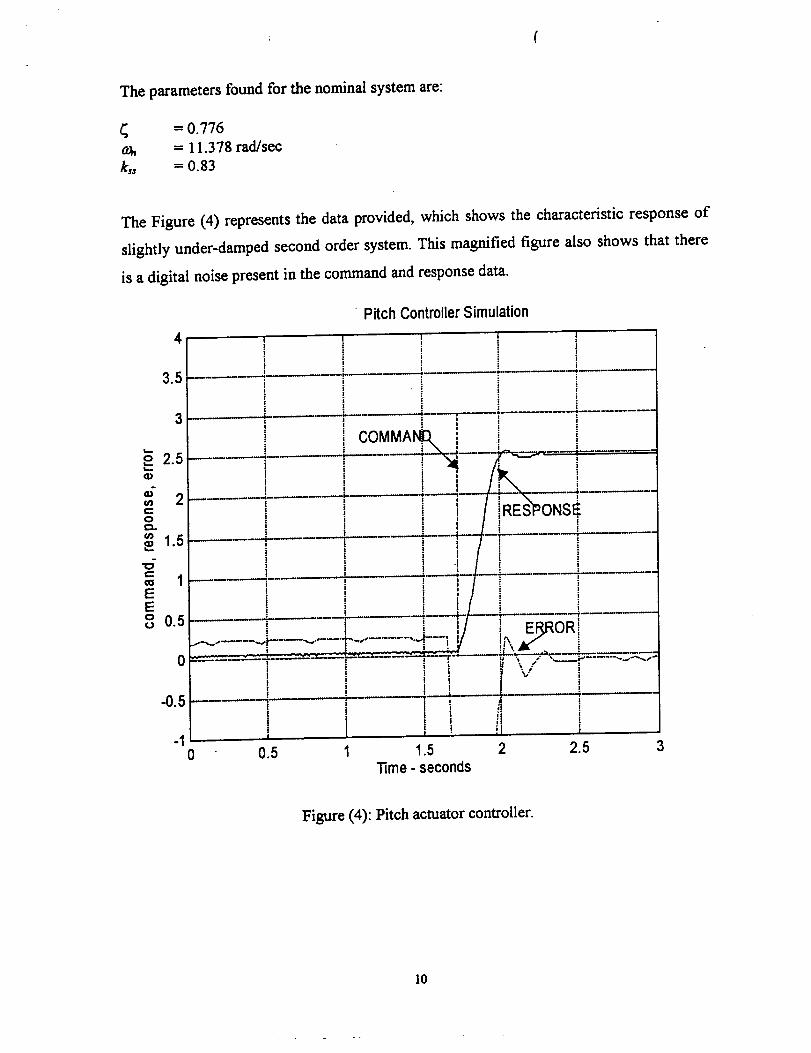
The parameters found for the nominal system are:

=0.776= 11.378 rad/sec

k. = 0.83

The Figure (4) represents the data provided, which shows the characteristic response of

slightly under-damped second order system. This magnified figure also shows that there

is a digital noise present in the command and response data.

• Pitch Controller Simulation

' I i ii. _ i. I

-O.5 ...... I

i-1 I

0 0.5

31-- i..... ,,.'- _ t T...... T/ i i COMMAND. i J J

' i i , i i ---

,..,.o_L-_-----J/ ,'.... ,-------4-"-,4----_---i_'i' _. /L" i.......L_ ' " '-#..:-"x,-'} I : •

• } I i i :m-2 ---_...... , ! , •

g / i i i i / iRESPONSEl " ' '} I

I : I . •I • • i i I

_= ,, = i -- '---I----------4--_ ---ff......_. I .U r---- ! t I / _ i

= ! : • i• I l i I

, ______.__!.--, ..... -;-----_ .--........ _-----1 L- ..... ._- , . ---/--'- .... ,

I ' ' J_L_L..... '1 i i ' i iE_ i i _ --

....

¢D 0 5 .... _ ....o • I--- ', I '. ',-/-- i" ERROR,'t...--.-..... ....I...-- .-.-- t.-.-' --.'f , g !_._ :r i ' .-'-- '" L __.'LD',.._---"-. "

N _ .... --< ÷ -"" I-=..... _ !...... :,-'_--7"_.._......."--.---i i i i ., _i k ,." I

/ i i ! , i v iI i II I iI i

i, i Ii ;i ii ii iI i ii

i _ ii '

1 2 2.5 31.5]]me - seconds

Figure (4): Pitch actuator controller.

10

Figure (5) shows the block diagram of the resulting discretized pitch actuator model. The

inner block shows the discrete version of the unity gain open loop transfer function, taken

as the direct Z transform, using sampling time T = 0.007875 seconds of the transfer

function:

2Y(s) co.

R(s) s_+ 2(_.s

(

which yields:

Y(z) _ 0.0037326

R(z) z _ - 1.8921z + 0.89209

Inputoonmm_

(from n_)

_1)o ¢

¢omnmnd

yO)

J-Vt_

Limit÷1-3.0

Gainl

Actuator

respor_z

f

Figure (5): Pitch actuator controller model - discrete transfer function (input and output

limited saturation protection).

11

The output of this transfer function is then limited to a _+3.0 degrees of travel before

feeding it back to close the loop. The switches shown in the Figure are used to set the

input to the transfer to zero, whenever the output of the transfer function is being driven

into the limit. The steady state gain appears as gain1 in the diagram and is applied to the

input command signal. Outputs are provided from the subsystem model to give actuator

response, actuator rate, and servo error [Ref: 11 and 13].

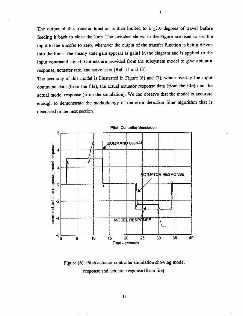
The accuracy of this model is illustrated in Figure (6) and (7), which overlay the input

command data (from the file), the actual actuator response data (from the file) and the

actuai model response (from the simulation). We can observe that the model is accurate

enough to demonstrate the methodology of the error detection filter algorithm that is

discussed in the next section.

Pitch ControllerSimulation

IiII

-60 10 15 30

I

l

1

l

5

t t

t

It!

!I

IIIlli

l

III

MODEL RESPONSEI !l !i !

t !tI I

20 25lime - seconds

IIIii

II

35 40

Figure (6): Pitch actuator controller simulation showing model

response and actuator response (from file).

12

3.5

32.5

1.5

8 o.s

0

Pitch ControllerSimulaUon

1 I i I I I I1 1 ! t t I !L L. i ) L___..J ....

i i I t 1 t it ! I t t ! t! t ! COMI_IAND SIGNALL ! t! t / / I\= ! . I

! I I l I_ i I..... "T..... T- I I I I t i

i , J t ! _AODEL I_ESPONSE Ii i i t fr,,_ i i i i

i I I / !_"_. ! ! ! !

i

--i .... ......s ) ! iE]. ., I ] i ,

.... 4t...... l-'-" il __/___ ! [ ! !___LiJ : ' l........ T'_--7 .....

"-_"-T-_T'-_ "I-'TTT'_T t T'--_T_- ! ....t I I i II t. ! ! t tt t t I !! 1 I t t tt t I I Y I t t t t! i t I 11 t i t t t

"--"il_--T-"_ i i I i ---I" .... I.....t i ! II! ! ! ! I lt I I I/I 1 ! I i It I t 14I I 1 I I t

i ' /I t 1 i I1.2 1.4 1.6 1.8 2 2.2 !.4 2.6 2.8 3

Time - seconds

Figure (7): Pitch actuator controller simulation - model response

and actuator response expanded view.

2.7 ERROR DETECTION FILTER

The error detection filter algorithm developed in this study works by comparing the

actual actuator response data to the response of the actuator subsystem model to the

actual actuator command data. From the output of the error detection filter, mean squared

error is computed. This is then compared with the variable threshold which is the "model

rate of change". If the mean squared error is less than the threshold value, error detect

will be "zero"; if the mean squared error value is more than the threshold value, error

detect will be "one", which triggers the fault detection system and a fault is detected.

13

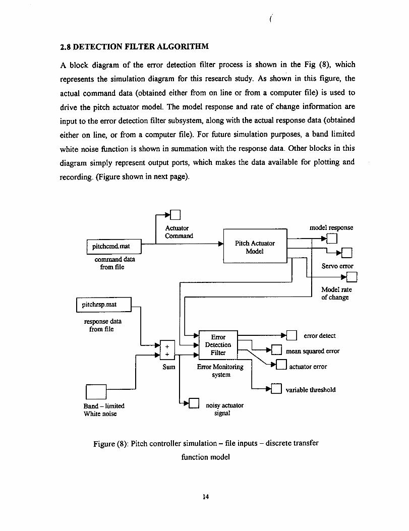
2.8 DETECTION FILTER ALGORITHM

A block diagram of the error detection filter process is shown in the Fig (8), which

represents the simulation diagram for this research study. As shown in this figure, the

actual command data (obtained either from on line or from a computer file) is used to

drive the pitch actuator model. The model response and rate of change information are

input to the error detection filter subsystem, along with the actual response data (obtained

either on line, or from a computer file). For future simulation purposes, a band limited

white noise function is shown in summation with the response data. Other blocks in this

diagram simply represent output ports, which makes the data available for plotting and

recording. (Figure shown in next page).

A_c_tor

pitchrsp.mat [response datafrom file

Sum

r-qBand - limitedWhite noise

ErrorDetection

Filter

kt ErrorMonitoring

system

noisy actuatorsignal

model response

Servo error

Model rate

of change

_lF-'] error detect

_,_mean squared error

actuator error

---_ variable threshold

Figure (8): Pitch controller simulation - file inputs - discrete transfer

function model

14

A detailed block diagram of only the error detection filter is shown in Fig (9). The error

between the system response data and the model response is squared and passed through

a discrete low pass filter. This provides and approximation to the expected (or average)

value of the mean squared error (MSE). This mean squared error value is then compared

to a threshold value and the error detection filter subsystem outputs a "zero" (meaning no

error) if the MSE is below the threshold, and a "one" (meaning an error is detected) if the

MSE is above the threshold [Ref: 11 and 13].

(

I detect I . _---_I,,_h,.,, ,d L :I:;"....... I Jresponse I _ Sumdatarrom I _um 3

Band- signa

O.05z

z-o._ IISquare Diecret |

Fcn I¢ow /

act

__ response

Discret

I.¢owpasschange 1 filter

Sum t

Constant

mean square

error

variablethreshold

.

Figure (9): Error Detection Filter - Recursive mean square - Discrete

approximation with threshold detection.

15

, (

A novel feature of this detection algorithm is the use of the model rate information to

dynamically adjust the error detection threshold. When the system is in steady state, it is

relatively easy to develop a model that accurately represents the system. However, when

the system is changing state rapidly, it is more difficult to accurately represent the

system, and more error should be tolerated to prevent false detects. Therefore, as shown

in the above Figure (9), a dynamic threshold is computed as follows:

T = Tt + y T 2

where:

T

Y

r/

r2

= Dynamic threshold

= Model rate of change

= Steady state threshold

= Rate sensitive factor

For this study, the simulation was run for various values of r_ and re and a optimum

values for these constants were achieved. It was found that rl = 0.02 and r2 = 0.04

worked well.

Finally, it should be noted that the dynamic threshold value itself must be passed through

a discrete digital filter matched to the one used to determine MSE, so that the phase lag

between the two signals remains matched. This greatly reduces false error detections and

allows for tighter setting of the threshold parameters.

16

f.

3- KALMAN FILTER FOR SIGNAL CONDITIONING

The use of Kalman filter is uniquely structured to condition raw data sequences in real-

time. In practice, the following are several cases that can be handled by the recursive

procedure:

i. The state variables can be measured directly; the object will be to filter the noise

from the raw measurement before comparison to the nominal model (false

detection will be the motivation here).

ii. The state variables can be measured directly. If several sensors are used to

measure the same variable, automatic weighing, based on statistical parameters of

the sensors, is applied by the Kalman filter to generate the "best estimate" of that

state variable.

iii. The state variable is impossible to measure directly; this case can be implemented

by finding the "best estimate" of those states by using measured data that can be

related by a known functional relationship to the desired state variables.

The block diagram of the Kalman filter process is shown in Fig (10).

u

MEASUREMENT ERRORS

q,

[ SYSTEM x

STATE

ESTIMATE

A PRIORI

INFORMATION

MEASURF_MENTS

Figure (10): Data flow for filtering process.

17

3.1 KALMAN FILTER FORMULATIONS [Ref: 5 and 6]

The random process to be estimated is modeled in the form of

Xt+ 1 -- CtXk 4" W k

The observation or the output of the system is given by,

gt = Htx* + vt

where:

xt

Wk

Zt

½

= (nx 1) process state vector

= (nxn) state transition matrix

= (nxl) vector, assumed to be white noise with known covariance structure.

= (rex 1) vector measurement (output)

(mxn) measurement to state matrix

= (mxl) measurement error assumed to be white noise with known covariance

structure.

The covariance matrices for wk and vk vectors are given by Qk and Rk. Assumption is

made that the initial estimate of the process is known at some point of time and this

estimate is based on the knowledge of the process. The estimation error is:

And the associated error covariance matrix is:

ek = xt - xk

where - x t - priori -estimate

(

.

With the known apriori estimate, the updated estimate is found:

P; = E[e, er l= E_x. - _, )(xk -_) r ]

where:

Kk = The Kalman filter gain

L

18

Now the error covariancematrix with theupdatedestimateisgiven by:

Pk = E[ek er] = El( x k - i, )(x, - xk )r ]

2, = 5q +Kk(z , -H,'k,)

In terms of noise covariance, Kalman filter gain (Kk) and Hk, the error covariance is given

by:

Pk = (I - KkHk )P_ (I - KkHk ) r + Kk RkKr

Now an expression is found for the computation of the Kalman filter gain (Kk) by

differentiating the above equation with respect to K since we wish to minimize the trace

of P as it is the sum of the mean-square errors of the estimates of all the elements of the

state vector. Hence Kk is given by:

Kk = Pf,-Hkr (HkPf,- Hkr + Rk)-,

A simple expression can be derived for error covariance matrix from above expressions:

Pk = (I- KkHk)P_

The next step is to make the optimal use of the measurement zk÷_. This is accomplished

by first updating the process estimate:

xL, = ¢:,

The error covariance matrix associated with updated process estimate is obtained by:

ell = xk+,- xL, = #kek+ wk

Thus we can write the expression for updated error covariance matrix as:

Pk-÷, = _kPk_ r +Q_

The above equations comprises of Kalman filter recursive equations.

19

Figure (11) shows the Kalman filter recursiv¢ loop structure. (.

Project ahead:A A

x,;. I = _*xk

pj,. = =¢,p, e r+ 0,

Enter prior esbmate _'and

its error covariance Po

Compute Kalman gain:

K, = P;rH_ (H,P;tH_* R,) -]

Compute error covariancefor updated estimate:

Pk = (I - Kj, H_)P k

rUpdate estimate with

measurement zk:A A A

x, = xj; + K, (z, - H,x;_)

Y

ZO, Z I . ...

,

Figure (11): Kalman filter recursive loop.

Now that we are in a stage where the system is' identified using the input output data, a

model has been developed along with a error detection system and error detection filter

algorithms, and a stage has been reached wherein we can study the optimal trajectories of

the model state variables, which will help us in validating the developed model in a

optimal sense. In other words, we can see from the plots of optimal trajectories with

varying initial conditions, that the states and the co-state variables of the model reach

steady state values quite quickly and also all the necessary optimal control conditions are

satisfied by the state equations. Here study has been made using the state equations and

2O

(

forming the Hamiltonian equation to see the behavior of the state and co-state

trajectories. This is discussed in detail in the next section.

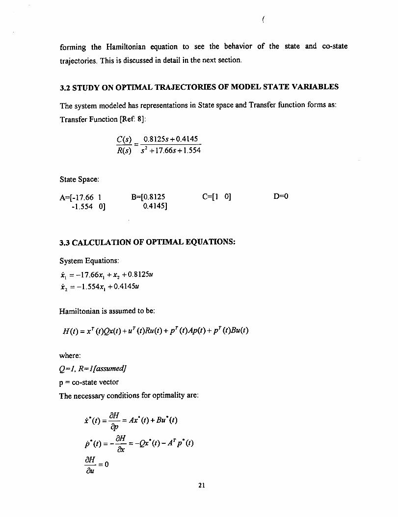
3.2 STUDY ON OPTIMAL TRAJECTORIES OF MODEL STATE VARIABLES

The system modeled has representations in State space and Transfer function forms as:

Transfer Function [Ref: 8]:

C(s)_ 0.8125s +0.4145

R(s) s _ +17.66s+1.554

State Space:

A=[-17.66 1 B=[0.8125

-1.554 0] 0.4145]

C=[1 0] D=0

3.3 CALCULATION OF OPTIMAL EQUATIONS:

System Equations:

_:1 = -17.66xl +x_ +0.8125u

_:_ =-1.554x I +0.4145u

Hamiltonian is assumed to be:

H(t)= x r (t)Qx(t)+u r (t)Ru(t) + pr (t)Ap(t) + pr (t)Bu(t)

where:

Q = I, R = 1[assumed]

p = co-state vector

The necessary conditions for optimality are:

$c"(t) = cgH= Ax"(t) + Bu"(t)@

OHp'(t) =

&c

OH_'-0

0u

- Ox'(t)- A_p" (t)

21

Since the system is of order 2x2, the number of optimal equations we get are four, which

are:

p_ :-17.66p_ + 2x_

p_ =-1.554p; +2x;

0H=0= 2u'(t)+O.8125p_(t)+O.4145p_(t)0u

simplifying =>

u °(t) = -0.40625p_" (t) - 0.20725p_ (t)

(

Substituting this optimal control in state equations, we get:

Yc_(t)=-17.66x_(t)+ x_(t)-O.33p_(t)-O.1684p:(t)

_ (t) = - 1.554xt" (t) - 0.1684p_" (t)- 0.0859p_ (t)

Hence the four optimal differential equations obtained are:

k_ (t) = - 17.66x_ (t) + x_(t)-O.33p_ (t)-O.1684p:(t)

_ (t) = -1.554x_ (t) - O. 1684p1" (t) - 0.0859p_ (t)

p_ =-17.66p_" + 2x_

p; =-1.554p; + 2x_

By solving the above differential equations by the method of finding eigenvalues and

eigenvectors, the resulting equations are in the form:

P_I

x_ i

Where the x's shown in the above equations are the eigenvectors of the differential

equations and 2 's are the corresponding eigenvalues.

A code is written in Matlab to generate various plots for the optimal states, optimal co-

states and optimal control trajectories for different initial conditions. The program is

shown below, by which for different initial conditions, various values of the constants

can be found out:

J

L

22

i (

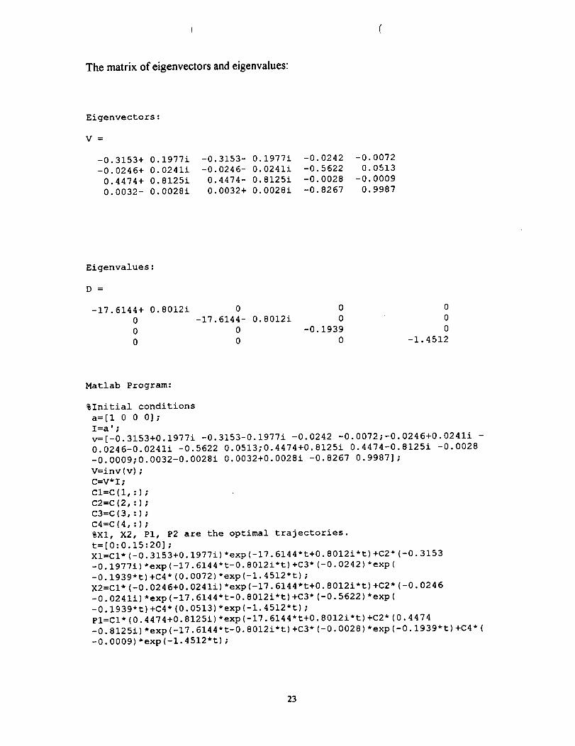
The matrix of eigenvectors and eigenvalues:

Eigenvectors:

V _"

-0.3153+ 0.1977i

-0.0246+ 0.0241i

0.4474+ 0.8125i

0.0032- 0.0028i

-0.3153- 0.1977i

-0.0246- 0.0241i

0.4474- 0.8125i

0.0032+ 0.0028i

-0.0242 -0.0072

-0.5622 0.0513

-0.0028 -0.0009

-0.8267 0.9987

Eigenvalues:

D ---

-17.6144+ 0.8012i 0 0 0

0 -17.6144- 0.8012i 0 0

0 0 -0.1939 0

0 0 0 -1.4512

Matlab Program:

%Initial conditions

a=[l 0 0 0];

I=a';

v=[-0.3153+0.1977i

0.0246-0.0241i -0.5622

-0.0009;0.0032-0.0028i

V=inv(v);

C=V*I;

CI=C(I, :) ;

C2=C (2, : ) ;

C3=C(3, :) ;

C4=C(4, : ) ;

%Xl, X2, PI, P2 are the

t=[0:0.15:20];

-0.3153-0.1977i -0.0242 -0.0072;-0.0246+0.0241i -

0.0513;0.4474+0.8125i 0.4474-0.8125i -0.0028

0.0032+0.0028i -0.8267 0.9987];

optimal trajectories.

Xl=Cl*(-0.3153+0.1977i)*exp(-17.6144*t+0.8012i*t)+C2*(-0.3153

-0.1977i)*exp(-17.6144*t-0.8012i*t)+C3*(-0.0242)*exp(

-0.1939*t)+C4*(0.0072)*exp(-l.4512*t);

X2=Cl*(-0.0246+0.0241i)*exp(-17.6144*t+0.8012i*t)+C2*(-0.0246

-0.0241i)*exp(-17.6144*t-0.8012i*t)+C3*(-0.5622)*exP(

-0.1939*t)+C4*(0.0513)*exp(-l.4512*t);

Pl=Cl*(0.4474+0.8125i)*exp(-17.6144*t+0.8012i*t)+C2*( 0.4474

-0.8125i)*exp(-17.6144*t-0.8012i*t)+C3*(-0.0028)*exp(-0.1939*t)+C4*(

-0.0009)*exp(-l.4512*t);

23

P2=Cl*(0.00320.0028i)*exp(17.6144*t+0.8012i*t)+C2*(0.0032+0.0028i)*exp(

-17.6144*t-0.8012i*t)+C3*(-0.8267)*exp(-0.1939*t)+C4*(0.9987)*exp(-

1.4512"t);

plot(t,Xl,'-',t,X2,' ',t, Pl,'-.',t, P2,'*')

title('Plot of Optimal Trajectories-State and Costate')

xlabel('time')

ylabel('Optimal Trajectories')

gtext('X1')

gtext('X2')

gtext('Pl')

gtext('P2')

gtext('Init Cond: XI=l,X2=l,Pl=0, P2=0')

(

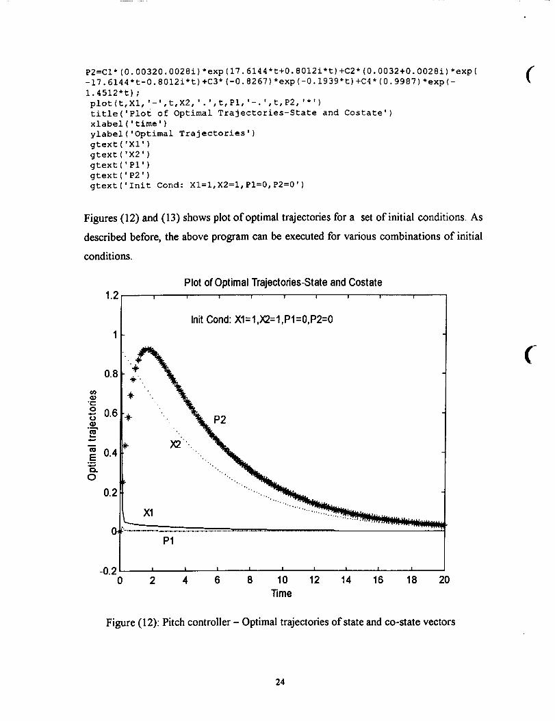
Figures (12) and (13) shows plot of optimal trajectories for a set of initial conditions• As

described before, the above program can be executed for various combinations of initial

conditions.

..-

O

Eo_

o

1.2

0.8

0.6

0.4

0.2

0_

Plot of Optimal Trajectories-State and CostateI I ! ! I ! I I I

Init Cond: X1=1IX2=l,Pl=O,P2=O

P2

X1

P1

-0.2 , , , , , i , , ,0 2 4 6 8 10 12 14 16 18 20

"rime

f

Figure (12): Pitch controller - Optimal trajectories of state and co-state vectors

24

1.2

Plot of Optimal Trajectories-State and Costate

I I I I ! ! I

0.8

._--0•.-. 0.6¢.)

0.4Eo_

0

0.2 X1

Init Cond: X1=1 ,X2=O,PI=O,P2=O

P1

P2

2 4 6 8 10 12 14 16 18 20

_me

Figure (13) • Optimal Trajectories of State and Co-state vectors with different

initial conditions.

Optimal trajectories can be plotted for various initial conditions. Figure (12) and (13)

shows the trajectories for two such initial conditions. We can observe, by initializing x=

and others equal to zero, that the optimal state and co-state trajectories reach steady state

value quite quickly (around 14 seconds). This provides a very good tool to determine the

behavior and to validate that the model is accurate enough.

25

(

f.

L

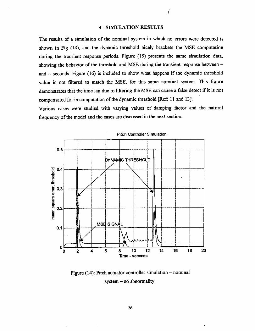
4 - SIMULATION RESULTS

The results of a simulation of the nominal system in which no errors were detected is

shown in Fig (14), and the dynamic threshold nicely brackets the MSE computation

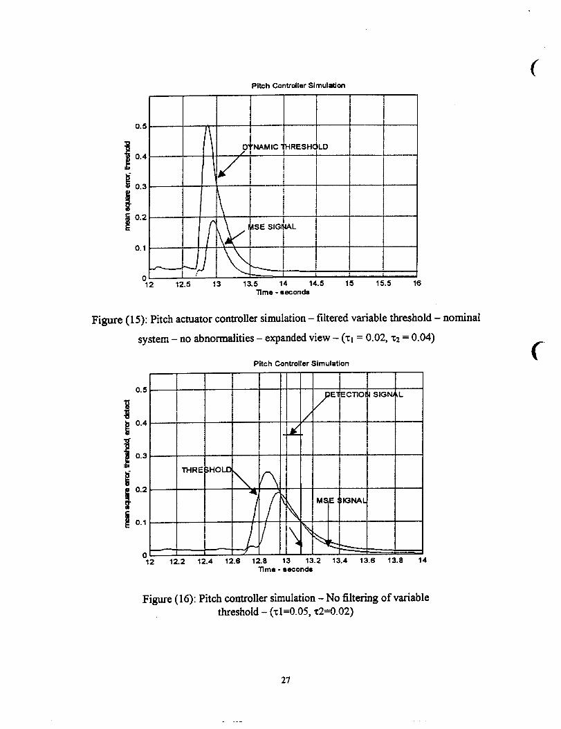
during the transient response periods. Figure (15) presents the same simulation data,

showing the behavior of the threshold and MSE during the transient response between -

and - seconds. Figure (16) is included to show what happens if the dynamic threshold

value is not filtered to match the MSE, for this same nominal system. This figure

demonstrates that the time lag due to filtering the MSE can cause a false detect if it is not

compensated for in computation of the dynamic threshold [Ref: 11 and 13].

Various cases were studied with varying values of damping factor and the natural

fi'equency of the model and the cases are discussed in the next section.

o0

Pitch Controller Simulation

_T I T T T r !

i t I [ !t • ]

! i i i I iI I

l [ DYNAMIC THRESHOLb! 1 1

j I

2 4 6 8 14 16 18 20• me-seconds

Figure (14): Pitch actuator controller simulation - nominal

system - no abnormality.

26

0.5

0.4

i0.3

i0.2

0.1

012 12.5

l

D_'NAMIC

// I

Pitch Controller Simulation

iI

i

i

i

i'HRESHC_LD

1!1

t

/ISE SIGI _AL

i i i i13 13.5 14 14.5 15 15.5 16

Time - seconds

(

Figure (15): Pitch actuator controller simulation - filtered variable threshold - nominal

system - no abnormalities - expanded view - (xl = 0.02, x2 = 0.04)

0.5

i0.4

0.3

0.2

0.1

012 12.2

THRE

Pitch Controller Simulation

1 i I

12.4 12.6 12.8 13 13.2 13.4 13.6 13.8 14Time - seconds

.

Figure (16): Pitch controller simulation- No filtering of variable

threshold - (x 1=0.05, x2=0.02)

27

It is noted here that the variations were made in the control parameters ¢ ca, and k,, to

test this new innovation threshold idea. These control parameters have been shown to

relate directly to the physical parameter of the System Under Test, therefore the detection

of an abnormal control parameter will indicate an abnormal value of the physical

parameter of the system under test.

Various figures were discussed to demonstrate the simulation of transient error in the

system. In one of the demonstrations, different cases have been studied by varying the

damping factor of the model. Figures show the actuator response, model response and

error detection flag in each case. During all transient response periods, the error detection

filter was able to successfully detect and announce the error. Various figures are also

included to show the dynamic threshold, MSE and the error detect flag in detail for all the

cases during the transient response periods.

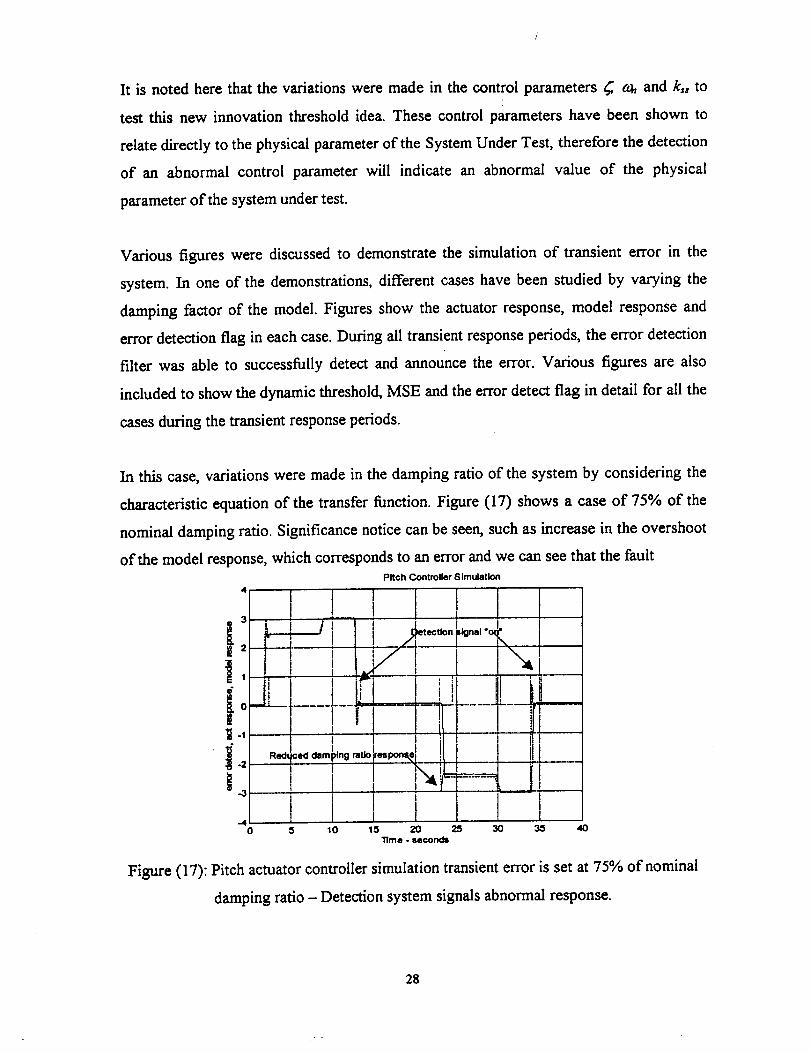
In this case, variations were made in the damping ratio of the system by considering the

characteristic equation of the transfer function. Figure (17) shows a case of 75% of the

nominal damping ratio. Significance notice can be seen, such as increase in the overshoot

of the model response, which corresponds to an error and we can see that the faultPitch Controller Simulation

' l| i_-4--Jt ' _,-.oo_..,-4: I

t I / I I "_1......!--r--FT .......T--!7--

i_ I I , --L 1 1 1

0 5 10 15 20 25 3O 35 4OTime - seconds

Figure (17): Pitch actuator controller simulation transient error is set at 75% of nominal

damping ratio - Detection system signals abnormal response.

28

detectionis "on". Figure (18) shows an expanded view of this which clearly shows that

there is a substantial increase in overshoot; hence the error filtered is triggered to give a

detection signal.

3.5

Pitch Controller Simulation

IRa] "O1'1

_ 3 R_duced ilampl, ratio r _;$_

2.5

l,;

_ 0.5 "

/

1.2 1.4 1.6 1.8 2 2.2Time - secorK:ls

01 2.4 2.6 2.8 3

Figure (18): Pitch actuator controller simulation- Expanded view of 75% _.

(

Also Figure (19) shows Dynamic threshold vs Mean square error signal (MSE) where

detection signal is on at the crossing of these two signals.

Pitch Controller Simulation

;ignal

0.5 I_

0.45 /-x - _Oel ectlon

o -'-it_ 0.35

0.3

\f\,\

tl°= /JI 0.15

0.1

.0.05

/ \×

1.8 2.4 2.6 2.6 31.2 1.4 1.6 2 2.2

Figure (19): Pitch actu_or con_oUer simul_ion - Dynamic threshold vs error signal of

75%_.

(

Similar results can be noticed when the natural frequency of the system is varied. In all

these cases, the error detection filter was able to detect and announce the error

29

successfully. We can also notice the changes in the model behavior; the transient

response of the model is oscillatory and settling time is substantially increased (in the

cases where the natural frequency is less than the nominal natural frequency). In the case

of co > co_, the error was detected to announce the change in the system parameters.

Overall, the error detection filter algorithm was able to determine the errors when the

nominal parameters of the system was changed in both the directions (increasing and

decreasing).

The basic idea behind all these different cases is the validation of the model and the

success &the error detection filter to detect and announce error due to the changes in the

system parameters. By this validation, we come to the conclusion that, if there is any

abnormal measurement input/output data coming from the actual system under test, the

model system parameters will change accordingly and due to these changes, the error

detection filter will detect the faults, hence the basic goal of fault detection is achieved.

30

(

C,

5. LIST OF REFERENCES

1. B. Friedland, ControlSystem Design, McGraw Hill Publications, 1986.

2. Charles L. Phillips and Royce D. Harbor, Feedback Control Systems, Third Edition,

Prentice Hall, 1996.

3. Roger W. Johnson, A Nenv Methodology for Launch�Spacecraft Vehicle Ground

Health Management, Monitoring and Test and Evaluation (White Paper), Institute

for Simulation and Training, University of Central Florida, April 29, 1994.

4. Roger W. Johnson, Sanjay Jayaram, Richard A Hull, A New Real-Time

Detection/Diagnosis Methodology for Automated Manufacturing, University of

Central Florida, 1998.

5. Arthur Gelb, Editor, Applied Optimal Estimation, The M.I.T Press, 1974.

6. Robert Grover Brown, Patrick Y.C. Hwang, Introduction to Random Signals and

Applied Kalman Filtering, Third Edition, John Wiley and Sons, Inc., 1997.

7. Ron Patton, Paul Frank, Robert Clark, Fault Diagnosis in Dynamic Systems -

Theory and Application, Prentice Hall International Inc., First Edition, 1989.

8. Donald E. Kirk, Optimal Control Theory - An Introduction, Prentice Hall

International Inc., First Edition, 1970.

9. Richard C. Doff, Robert H. Bishop, Modern Control Systems, Addison Wesley

Longman Inc., Eighth Edition, 1998.

10. Bernard Friedland, Maximum Likelihood Failure Detection of Aircraft Flight

Control Sensors, Journal of Guidance, Control and Dynamics, Vol. 5, No. 5, 1982,

pp. 498-503.

31

11. John N. Little and Alan J. Laub, Control System Toolbox for Use with MATLAB,

The Math Works Inc., Prentice Hall, 1996.

12. Lennart Ljung, System Identification Toolbox for Use with MATLAB, The Math

Works Inc., Prentice Hall, 1997.

13. The Math Works Inc., SIMULINK- Dynamic System Simulation Software, User's

Guide, 1993 and 1997.

14. The Math Works Inc., MATLAB - High Performance Numeric Computation and

Visualation Software, 1993.

(

f

t.

32

APPENDIX - A

! (

(

f-

ooo_ .... ....

....... . ...... o .... _°.

I I I I

°°°_ ..................

.°

.°.

I I

.._°

IIII II

(-

C

IC O_ W8 SI 1_0 86.