A New Data Mining Model for Hurricane Intensity Prediction

Yu Su, Sudheer Chelluboina, Michael Hahsler and Margaret H. Dunham

Department of Computer Science and Engineering

Southern Methodist University

Dallas, Texas 75275–0122

{mhahsler, mhd}@lyle.smu.edu

Abstract—This paper proposes a new hurricane intensityprediction model, WFL-EMM, which is based on the datamining techniques of feature weight learning (WFL) andExtensible Markov Model (EMM). The data features usedare those employed by one of the most popular intensityprediction models, SHIPS. In our algorithm, the weights ofthe features are learned by a genetic algorithm (GA) usinghistorical hurricane data. As the GAs fitness function we usethe error of the intensity prediction by an EMM learned usinggiven feature weights. For fitness calculation we use a techniquesimilar to k-fold cross validation on the training data. The bestweights obtained by the genetic algorithm are used to buildan EMM with all training data. This EMM is then applied topredict the hurricane intensities and compute prediction errorsfor the test data.

Using historical data for the named Atlantic tropical cyclonesfrom 1982 to 2003, experiments demonstrate that WFL-EMMprovides significantly more accurate intensity predictions thanSHIPS within 72 hours. Since we report here first results, weindicate how to improve WFL-EMM in the future.

Keywords-Hurricane, intensity prediction, Markov chain

I. INTRODUCTION

Hurricanes are tropical cyclones with sustained winds of

at least 64 kt (119 km/h, 74 mph) [1]. On an average,

more than 5 tropical cyclones become hurricanes in the

United States each year causing great human and economic

losses [1]. The major issues in forecasting hurricanes are

predicting their tracks of movement and their intensities.

Intensity is defined as the maximum average windspeed

over a predefined time window (1 or 10 minutes usually).

Compared with prediction of track movement, intensity

prediction is still relatively inaccurate, which may be due

to lack of understanding of all the features that influence

the intensity of hurricanes [2].

This paper proposes a new algorithm for hurricane inten-

sity prediction based on the techniques of weighted feature

learning and EMM. Extensible Markov Model (EMM) [3]

is a dynamic streaming data learning model which pro-

vides efficient methods for outlier detection, pattern analysis

and future state prediction. In this paper we propose a

new algorithm called Weighted Feature Learning EMM

(WFL-EMM) to predict the future intensity of hurricanes

This work was supported in part by the U.S. National Science FoundationNSF-IIS-0948893.

by combining a novel weighted feature learning technique

with EMM. Compared with EMM, WFL-EMM provides

stronger learning abilities as the genetic algorithm learning

component of WFL-EMM actually learns the best EMM for

a set of EMMs defined by different feature weights. EMM

assumes that the input data stream is composed of vectors

of numeric values. The size of the vectors is determined

by the number of features. In this basic case, the EMM

assumes that all features are weighted the same and have the

same importance to the application being studied. However,

we know that for hurricane intensity prediction, all features

are not equal. Rather than treating features equally, WFL-

EMM gives a weight for each feature and these weights

form a weight vector, u, for all the features. A u which

gives the lowest error is then found during the training

process. To locate a good solution, a genetic algorithm [4]

is introduced in our prediction model. Then an EMM is

constructed based on this u and the prediction is made

by using EMM prediction techniques. Experimental results

demonstrate that WFL-EMM is a robust and stable future

state prediction model.

The rest of this paper is organized as follows. The

next section introduces related work on tropical cyclone

intensity prediction. Section III describes the dataset we

used for training and testing of WFL-EMM. Section IV

and Section V give details of EMM techniques and the

genetic algorithm used for learning weights, respectively.

Section VI discusses the experiments. We conclude the paper

in Section VII.

II. RELATED WORK

Many models have been proposed to predict hurricane

intensity. Most of these models are based on regression

and probabilistic methods. Some examples of statistical

prediction models are SHIFOR [5], GFDL [6] and SHIPS [7]

[8] [9]. SHIFOR was the first operational intensity prediction

model. It uses the statistical relationships between clima-

tological and persistence features to predict the hurricane

intensity over water. GFDL (Geographical Fluid Dynamics

Laboratory) model became operational in 1995. It uses initial

cyclone conditions to predict the intensity. SHIPS (Statistical

Hurricane Intensity Prediction Scheme) was developed by

using a multiple linear regression technique with climato-

2010 IEEE International Conference on Data Mining Workshops

978-0-7695-4257-7/10 $26.00 © 2010 IEEE

DOI 10.1109/ICDMW.2010.158

98

2010 IEEE International Conference on Data Mining Workshops

978-0-7695-4257-7/10 $26.00 © 2010 IEEE

DOI 10.1109/ICDMW.2010.158

98

logical, persistence, and synoptic predictors for predicting

intensity changes of Atlantic and eastern North Pacific basin

tropical cyclones. In recent years, some research has applied

data mining techniques to improve the intensity prediction.

One example of such research is [10], which formulates

intensity prediction as a supervised data mining problem and

examines two approaches (particle swarm optimization and

association rules) to discover the patterns in hurricane data.

In recent decades, Markov chain techniques have been

gaining popularity in meteorological circles for forecasting

intensity, track movement and risk assessment [11]. Usually,

in intensity prediction approaches, a Markov chain is defined

as a process of collecting random variables indexed by time.

It implies that the current observation only depends on the

previous states, where a state is a collection of similar

observations. Widely used first-order models assume that

the current state only depends on the previous state. For

instance, let st denote a current state. Then st only depends

on the state st−1, where t − 1 indicates the previous time

interval of t. One early research of intensity prediction based

on Markov chains is [12], which proposes transition proba-

bility analysis to predict the intensity changes to forecast the

hurricane intensity. [13] proposes a probabilistic model for

determining sudden changes at unknown times in records

involving annual hurricane counts. [14] introduces a hybrid

model which combines a climatology-based Markov storm

model with a dynamic decision making for explicit anticipa-

tion of improving the forecasts and fine tuning the decisions

to reduce the total risk and unnecessary preparations for false

warnings.

A. SHIPS Model

Among these intensity prediction models SHIPS [7] [8]

[9], after decades of development, is still one of the best-

performing [2] [10]. The first version of SHIPS (Statistical

Hurricane Intensity Prediction Scheme) is introduced by [7],

which proposes a statistical model for predicting intensity

changes of Atlantic tropical cyclones. An updated version

of SHIPS [8] was also developed for intensity prediction of

the eastern North Pacific basin. The model was developed

by using a multiple linear regression technique with climato-

logical, persistence, and synoptic predictors. Each hurricane

is described by time ordered data indexed with 0h, 12h,

24h, . . ., where time label t indicates the future state after

t 12-hours time intervals from the zero state (first state of a

hurricane). All predictors collected at time t form a feature

vector dt = 〈d1, d2, . . . , dn〉. SHIPS then creates a data set

to learn a multiple linear regression model. For each t the

interdependent variables are dt and the dependent variables

are the intensities in the future (at t+1, t+2, . . . ). For each

time in the future an independent linear regression model is

learned.

Eleven predictors (ten are linear predictors and one is

quadratic predictor) are used in the first version of SHIPS

(1994) [7]. Predictors are removed and added depending on

the performances of the model for different seasons. In 1997,

a considerable change was made by adding and adjusting

features to include the decay over the land. But this resulted

in errors for the cases where a hurricane moves back over

the water. To compensate for this problem, a new version of

SHIPS [9] was proposed by adding the dependent features

which are the differences of intensity between 12 hours. [9]

also increases the forecast period from 3 to 5 days.

III. DATASET DESCRIPTION

There are 37 predictors used in SHIPS 2005 [9]. Among

these, we use 16 predictors (4 are quadratic features) to

evaluate our prediction model. The dataset is formed by time

ordered 12 hour interval records and contains the hurricane

data from seasons 1982 to 2003. Table I gives the description

of predictors used in our model. VMAX is the current

maximum wind intensity in kt. POT is the difference of

maximum possible intensity (MPI) to the initial intensity.

MPI is given by the empirical formula from [7]. The

predictor PER is the change in the intensity with which the

intensification for the next 12 hours can be estimated. ADAY

is the climatological feature that is evaluated before the

forecast interval. ADAY is given by the formula described

in [9]. SHRD is averaged along the cyclone track. LSHR

is a quadratic feature given by the product of vertical shear

feature and the sine of the initial storm latitude. T200 is

the 200-mb temperature averaged over a circular area with

radius of 1000 km centered on initial cyclone position. U200,

Z850 are the linear synoptic predictors. In [8], SPDX is

considered to be a significant feature which distinguishes the

cyclones easterly versus westerly currents. VSHR is also a

quadratic predictor given by the product of maximum initial

intensity and SHRD. RHHI feature is added to represent the

Sahara air layer effect. VPER is a quadratic feature and it is

given by the product of PER and maximum initial intensity.

IV. EMM FOR PREDICTION

Extensible Markov Model (EMM) [3] has the advantage

of using a distance-based clustering technique for modeling

spatial and temporal data. EMM is an efficient model that

maps spatial-temporal events to states of a Markov chain

and provides a dynamical graph-based structure to model the

streaming data when the complete set of states is unknown.

Let GEMM = 〈V,E〉 denote an EMM, where V is a set of

vertices which are centers of clusters of data points and E

is a set of directed edges which indicate the state transitions

between these clusters. Each vertex has a counter and each

edge has a weight associated with it. To generate an EMM,

two basic algorithms are introduced in [15].

1) EMMCluster defines an operation for matching a new

input data point dt+1 at time t + 1 to the cluster set

V in GEMM of time t. If there exists a cluster vi ∈V such that the distance dist(vi,dt+1) is less than a

9999

100100

B. Genetic Algorithm Learning Process

After introducing the weights for different features, a real

number ui ∈ [0, 1] is assigned for the ith feature to indicate

the contribution of this attribute for the prediction. ui =1 implies that ith feature is important and ui = 0 means

that the ith feature is ignored for intensity prediction. For

n attributes and a vector u = 〈u1, . . . , un〉, we see that the

search space is [0, 1]n.

To find a u which gives a close to optimal prediction

error we apply a genetic algorithm [4]. GAs try to locate

the solution with the best fitness for the given problem. For

our algorithm, we define fitness as the smallest root means

square intensity prediction error (see formula 1). We encode

possible solutions, the weight vector u, as a binary string

which is called for GAs the chromosome. Here all weights

are converted into binary numbers (as often for GAs we

use also Gray code here) and then the binary numbers are

concatenated into one string of bits. If we encode each of the

n feature weights ui using m bits, then a chromosome will

be a bit string with mn bits. This results in a search space

size of 2mn. Suppose m = 1, then the possible value of ui is

0 or 1. This reduces the problem to a pure attribute selection

problem. We choose m = 8, which gives 256 possible values

(between 0 and 255) for each ui, where 0 indicates that ith

attribute is ignored. For the n = 16 features in our intensity

prediction data set we get for m = 8 a very large search

space size of 2128.

GAs are based on the idea of random evolution with

survival of the fittest. GAs always have a population ζ of

chromosomes. The initial population ζ0 is populated with

randomly generated chromosomes. Then in each evolution-

ary step, a new population is created from the old population

using several genetic operators. Here we use crossover,

mutation and inversion. The GA stops when the error rate

converges (i.e., the improvement of the error rate falls below

a set value).

For crossover, two chromosomes are selected randomly

from ζi with a probability proportional to their fitness.

This makes sure that fitter chromosomes are chosen more

frequently. One or more break points are randomly selected

over the parents and the offspring is created as a mixture

of the parents (i.e., all bits from the first parent till the

break point and then all remaining bits from the second

parent). Following the crossover operation, the mutation

operation randomly alters one or more bits in the offspring

based on a given probability to allow for local search for

better solutions. Although this given probability usually is

quite small, which means this occurs very infrequently,

mutation operation is believed to be one of main driving

forces for evolution. After considering the length of the

chromosome used in predication process, rather than using

only one mutation point, we alter multiple bits in the new

born offspring. We also use the inversion operation, which

randomly selects a break point in a chromosome and then

exchanges the position of the two pieces. Then the GA

evaluates the fitness of the new chromosomes by calculating

the error (formula 1) and places the obtained chromosome

into ζi+1.

In our GA algorithm, the following steps are followed.

Assume the population size of each generation is τ . For the

initial generation ζ0 (i = 0), the chromosomes are generated

randomly. For each chromosome in ζi we extract the feature

weight vector u. We weight the training data using u and

then use a k-fold cross validation technique with this data

by always learning an EMM with k − 1 parts of the data

and calculating the error for the remaining data. The fitness

is then calculated as the average of the obtained k errors.

After computing the fitness for all chromosomes in ζi, the

GA creates the chromosomes for generation ζi+1 using the

genetic operations described above. We repeat this process

until a stopping condition |Ei+1−Ei| < ǫ is satisfied. Ei and

Ei+1 denotes the average fitness for the i + 1th generation

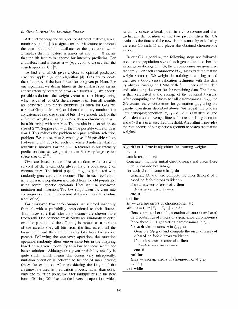
and ǫ > 0 is a user specified threshold. Algorithm 1 provides

the pseudocode of our genetic algorithm to search the feature

weights.

Algorithm 1 Genetic algorithm for learning weights

i← 0smallesterror ←∞Generate τ number initial chromosomes and place these

initial chromosomes into ζifor each chromosome c in ζi do

Generate GEMM and compute the error (fitness) of c

based on k-fold cross validation

if smallesterror > error of c then

Bestchromosomes← c

end if

end for

Ei ← average errors of chromosomes ∈ ζiwhile i = 0 or |Ei − Ei−1| < ǫ do

Generate τ number i+1 generation chromosomes based

on probabilities of fitness of i generation chromosomes

Place these i+ 1 generation chromosomes in ζi+1

for each chromosome c in ζi+1 do

Generate GEMM and compute the error (fitness) of

c based on k-fold cross validation

if smallesterror > error of c then

Bestchromosomes← c

end if

end for

Ei+1 ← average errors of chromosomes ∈ ζi+1

i← i+ 1end while

101101

102102

103103

104104

[10] J. Tang, R. Yang, and M. Kafatos, “Data mining for tropicalcyclone intensity prediction,” Sixth Conference on CoastalAtmospheric and Oceanic Prediction and Processes, January2005, session 7, Tropical Cyclones.

[11] M. Drton, C. Marzban, P. Guttorp, and J. T. Schaefer, “Amarkov chain model of tornadic activity,” Monthly WeatherReview, vol. 131, no. 12, pp. 2941–2953, 2003.

[12] L. Leslie and G. Holland, “Predicting changes in intensity oftropical cyclone using markov chain technique,” 19th Conf.on Hurricanes and Tropical Meteorology, pp. 508–510, 1991.

[13] J. B. Elsner, X. Niu, and T. H. Jagger, “Detecting shifts inhurricane rates using a markov chain monte carlo approach,”Journal of Climate, vol. 17, no. 13, pp. 2652–2666, 2004.

[14] E. Regnier and P. A. Harr, “A dynamic decision model appliedto hurricane landfall,” Weather and Forecasting, vol. 21, no. 5,pp. 764–780, 2006.

[15] Y. Meng and M. H. Dunham, “Mining developing trends ofdynamic spatiotemporal data streams,” Journal of Computers,vol. 1, no. 3, pp. 43–50, June 2006.

[16] S. Shankar and G. Karypis, “A feature weight adjustmentalgorithm for document categorization,” in In Proceedings ofthe Sixth ACM SIGKDD International Conference on Knowl-edge Discovery and Data Mining (ACM SIGKDD 2000),2000.

105105