Working Paper 2009:15Department of Economics

A new consumer price indexthat incorporates housing

Anders Klevmarken, Olle Grünewald andHenrik Allansson

Department of Economics Working paper 2009:15Uppsala University November 2009P.O. Box 513 ISSN 1653-6975 SE-751 20 UppsalaSwedenFax: +46 18 471 14 78

A NEW CONSUMER PRICE INDEX THAT INCORPORATES HOUSING

ANDERS KLEVMARKEN, OLLE GRÜNEWALD AND HENRIK ALLANSSON

Papers in the Working Paper Series are published on internet in PDF formats. Download from http://www.nek.uu.se or from S-WoPEC http://swopec.hhs.se/uunewp/

1

A new consumer price index that incorporates housing

Anders Klevmarken1, Olle Grünewald and Henrik Allansson2

November 3, 2009

A long lasting controversy in Sweden as well as internationally is how to best estimate a price on the

services of owner occupied housing in a consumer price index. There is no international consensus

and different approaches have been adopted. In this paper we use a true cost-of-living index

suggested by one of the authors, apply the model to Swedish data and compare the results to the

current Swedish CPI. We also show that within the economic model underlying the true cost-of-living

index, alternative operationalizations of the index give rather different results. The choice between

these alternatives depends upon the primary purpose of the index.

Keywords: Price index, cost-of-living index, compensation index, price of housing services

JEL

: C43, D91

1 Department of Economics, Uppsala University, Sweden; Email: anders.klevmarken@nek.uu.se 2 Statistics Sweden, Stockholm, Sweden; Email: Olle.Grunewald@scb.se and Henrik.Allanson@scb.se . The views expressed are those of the authors and do not necessarily reflect the policies of Statistics Sweden or the views of other staff members.

2

1.

In many countries housing as a share of private consumption is as much as 25 to 30 percent. The

price of housing services is thus a major component of a consumer price index. Depending on

country these services are to a large extent generated from owner occupied dwellings for which

there is no readily observable price. There is no generally acceptable practice to measure the price of

these housing services. In some countries they are represented by an index of rented apartments, in

other countries attempts are made to estimate some kind of user cost, and in a few countries there is

no index at all for owned housing, which implicitly means that the price of these services is assumed

to follow the general CPI.

Introduction

The literature on price index numbers distinguishes between a few major approaches to measure the

price of services from durable goods: the acquisition approach, the rental equivalence approach, the

payment approach and the user cost approach. The acquisition approach is used for nondurables but

typically also for durables with the exception of owner occupied housing. For most purposes of a CPI

one prefers to measure changes in the price of the services derived from a house rather than

changes in the price of the house as such. The same argument could have been used for any major

durable consumption good, such as vehicles, but the international convention is to use the

acquisition approach in this case. The motivation is probably a desire to avoid all the problems with

the user cost approach and with weak rental markets. In many countries the rental market for

detached houses is very thin, only covering a selected sample of houses. The rental equivalence

approach is thus not operational in these countries. In the payments approach one measures cash

out-payments for the cost of operating an owner occupied dwelling, but ignores depreciation and the

opportunity cost of holding the equity in the owner occupied dwelling.

Many theoretical economists prefer to follow the user cost approach. It recognizes that the purchase

of a house is both a consumption and an investment decision. The purchase price can be

decomposed into one component which represents the services derived from the house in a given

period (depreciation), and another – the end of period value - which is an investment. As an investor

the house owner wants a return on his investment, which can be seen as an opportunity cost. The

practical implementation of the user cost approach involves the estimation of rather elusive

concepts such as; the opportunity cost of the investment, the depreciation of a house, the subjective

3

interest rate that equalizes amounts in the beginning and the end of a period, purchase prices of

constant quality houses, and in some user cost definitions expected future purchase prices. There are

many ways to estimate these concepts and incorporate them in an index formula, one not

necessarily better than another. The resulting index might depend very much on the specific solution

chosen. Typically empirical implementations of the user cost approach result in indices that become

rather volatile.

Some practitioners view a consumer price index simply as a weighted mean of price relatives. The

problem of computing such an index involves the definition of an index formula, the definition of

commodities, finding methods to measure the corresponding prices, and defining the weights. There

are obviously infinitely many combinations of these entities which result in indices with different

properties. In the so called axiomatic approach a number of plausible properties (axioms) are

specified a priori and only indices which satisfy these axioms belong to the feasible set of indices.

Depending on the axioms chosen and the definitions of the entities there is no guarantee for a

nonempty set, nor for a small set. The major problems of this pragmatic approach are, however, that

it is completely unrelated to the behavior of consumers and markets, and also to the major uses of a

CPI.

The theory of the true cost of living index is an attempt to meet these objections and give index

theory a foundation in classical consumer choice theory. In his pioneering work Konüs (1924, 1939)

used a simple static model of consumer optimization. This model only includes nondurables, and it

must be generalized to accommodate durables and to allow the consumer to optimize over more

than one period, before it can become a useful tool to define a true cost of living index that

incorporates housing. Klevmarken (2009) has recently suggested a semi dynamic model of consumer

behavior that incorporates the demand for housing and is consistent with the general purpose of a

consumer price index. He used this model to derive a true cost of living index and showed, given

certain assumptions, that there are conventional Laspeyres approximations which can be computed

with the information usually collected at a statistical bureau.

Using Swedish data we demonstrate in this paper how Klevmarken’s index can be implemented and

compare the results to the current Swedish CPI. It turns out that economic theory and the

accompanying approximations do not yield a unique index. There is still scope for strategic choices

4

which become numerically important. We discuss these choices against the background of the most

important uses of the Swedish CPI. Our results as well as this discussion raise the issue of revising the

current index.

Before reviewing our results we summarize the assumptions and properties of the index proposed in

Klevmarken (2009) and discuss alternative variants. These sections draw heavily on Klevmarken

(2009). We then continue with a summary of the properties of the current Swedish CPI with a focus

on the subindex for housing services. Then follows a description of the practical implementation of

Klevmarken’s index, i.e. the choice of price and weight data, after which we are ready to present our

comparative results and discuss their implications. The empirical implementation draws on

Grünewald, Lundin & Allansson (2009).

2.

A true cost-of-living index as a basis for a consumer price index should be able to answer a rather

simple question: “What income is needed today to compensate for a price change today?” Although

economic decisions about housing typically both influence immediate utility as well as future utility,

we do not necessarily need a multiperiod optimization model to capture the most important features

of this decision situation and at the same time be able to answer the basic CPI question. Klevmarken

(2009) assumes that time is discrete and that a time period is homogenous in the sense that prices

do not change in a period, only between periods. The consumer is assumed to maximize the

following utility function subject to a budget constraint,

A true cost-of-living index

0( , , , , ( ), ( ));h m h r A MU q q q q g A g Mλ+q (1)

where q is a vector of volumes of non-housing commodities, 0hq the initial stock of own housing and

mq the volume of repair and maintenance. mh qq λ+0 then represents the housing stock available for

current consumption including any maintenance and repair. λ is a factor that translates maintenance

5

and repair into house value. A value different from one allows for more or less value enhancing

repair and maintenance activities.3

In principle one could represent the services the consumer obtains from his own house by the

product of a depreciation factor and the stock, but for simplicity this factor is absorbed into the

utility function.4hq is the terminal stock of own housing representing the quantity of house which

has a future consumption value. Through the utility function the consumer attaches a current value

to the future services a house is expected to provide. There is thus a trade off in utility between using

a house today and using it tomorrow. qr is the volume of rented housing services. Most consumers

will have utility functions with properties such that they will either choose a house or an apartment,

but we do not exclude the possibility of having both.

Finally, A is financial assets at the end of a period, and M mortgages and loans. Financial assets can in

the future be used for consumption and having assets for this reason enhances utility today. Their

contribution to utility depends on the expected future real return on assets. The function (.)Ag

represents the consumer’s expectations in this respect. Mortgages and loans do not contribute to

direct utility, only indirectly through the higher consumption volumes of goods and services they

enable. However, higher liabilities increase the consumer’s exposure to market risks. He may also

become more sensitive to health related risks in the sense that illness and accidents may cause

difficulties in satisfying contracted interest payments and payments towards the principal. High multi

3 For simplicity in order not to complicate all formulas we also include in qm the services and material needed to

operate a house such as heating. It is not always easy to make a clear distinction between these goods and

services and those used for maintenance. For instance, if a house is not heated in a Nordic climate it will quickly

wear down.

4 In fact, the services obtained from a given house will in general differ from one consumer to another

depending on the consumers’ preferences. It follows that the services a consumer obtains from a house need

not be the same as a market determined depreciation.

6

period mortgages and loans also constrain future consumption possibilities. In a multi period model

future payment to service a loan are, like other expenditures, usually included in the budget

constraint, and thus determine the consumer’s optimization. The model specified in this paper is not

dynamic in this sense, the budget constraint only includes current expenditures – see below. Instead

we assume that the consumer evaluates the future budget impact of a loan taken today and

translates it into current disutility. There are thus two reasons to include liabilities as an argument in

the utility function: the disutility of increased risk and the disutility of future consumption

constraints. None of these two effects depend on the nominal size of the loans and mortgages, but

rather on a measure relative to collateral, assets owned by the consumer and his earnings capacity.

The function gM(.) makes this translation into a “real” measure. To simplify and focus on the housing

market Klevmarken (2009) assumes that mortgages and loans are primarily or exclusively taken to

finance housing. The collateral of a mortgage is then the market value of an owned home, and a

natural measure of the risk to which the consumer is exposed is the mortgage share M/phqh. It is thus

assumed that,

( )Mh h

Mg M Mp q= = (2)

It is futher assumed that the consumer expects a future real return r on financial assets. It then

follows that,

( ) (1 )Ag A A r A= + = ; (3)

7

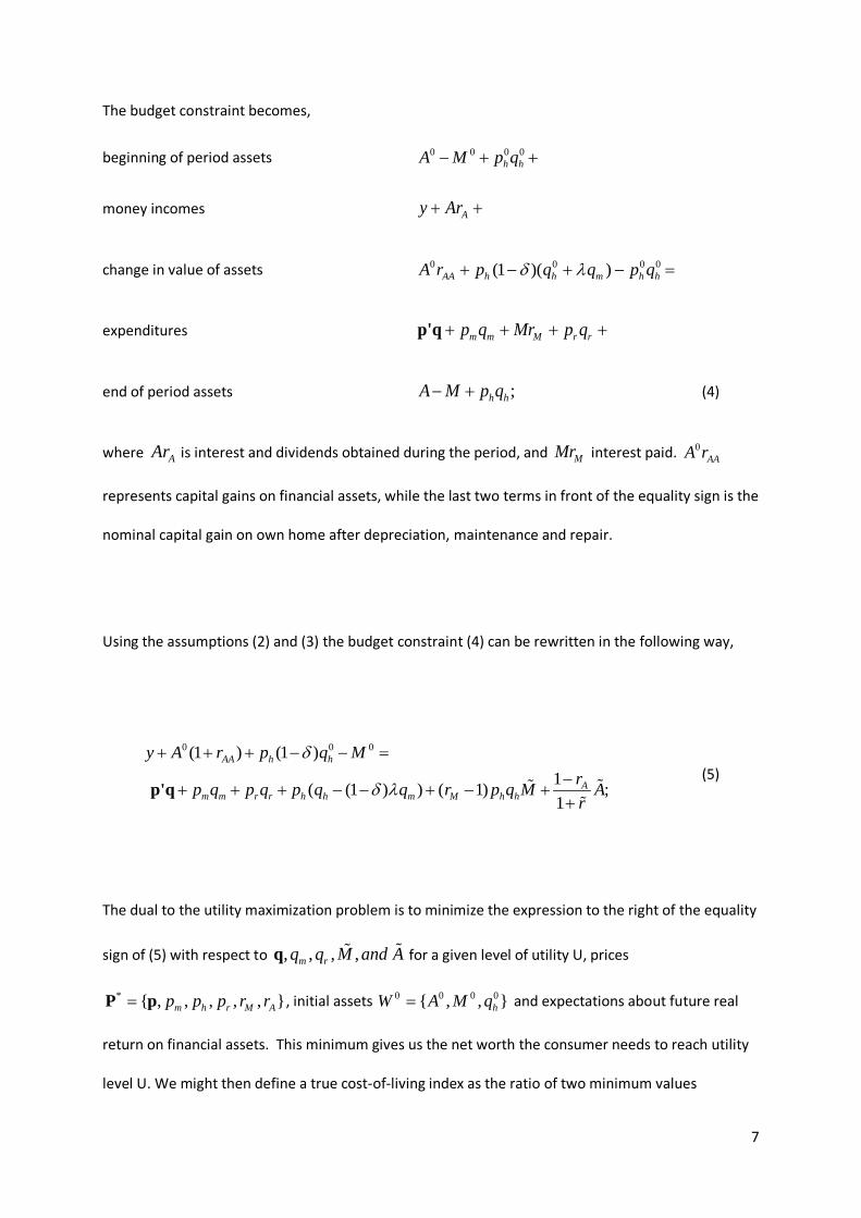
The budget constraint becomes,

beginning of period assets 0 0 0 0h hA M p q− + +

money incomes Ay Ar+ +

change in value of assets 0 0 0 0(1 )( )AA h h m h hA r p q q p qδ λ+ − + − =

expenditures m m M r rp q Mr p q+ + + +p'q

end of period assets ;h hA M p q− + (4)

where AAr is interest and dividends obtained during the period, and MMr interest paid. 0AAA r

represents capital gains on financial assets, while the last two terms in front of the equality sign is the

nominal capital gain on own home after depreciation, maintenance and repair.

Using the assumptions (2) and (3) the budget constraint (4) can be rewritten in the following way,

0 0 0(1 ) (1 )1( (1 ) ) ( 1) ;1

AA h h

Am m r r h h m M h h

y A r p q Mrp q p q p q q r p q M Ar

δ

δ λ

+ + + − − =−

+ + + − − + − ++

p'q

(5)

The dual to the utility maximization problem is to minimize the expression to the right of the equality

sign of (5) with respect to , , , ,m rq q M and Aq for a given level of utility U, prices

* { , , , , , }m h r M Ap p p r r=P p , initial assets 0 0 0 0{ , , }hW A M q= and expectations about future real

return on financial assets. This minimum gives us the net worth the consumer needs to reach utility

level U. We might then define a true cost-of-living index as the ratio of two minimum values

8

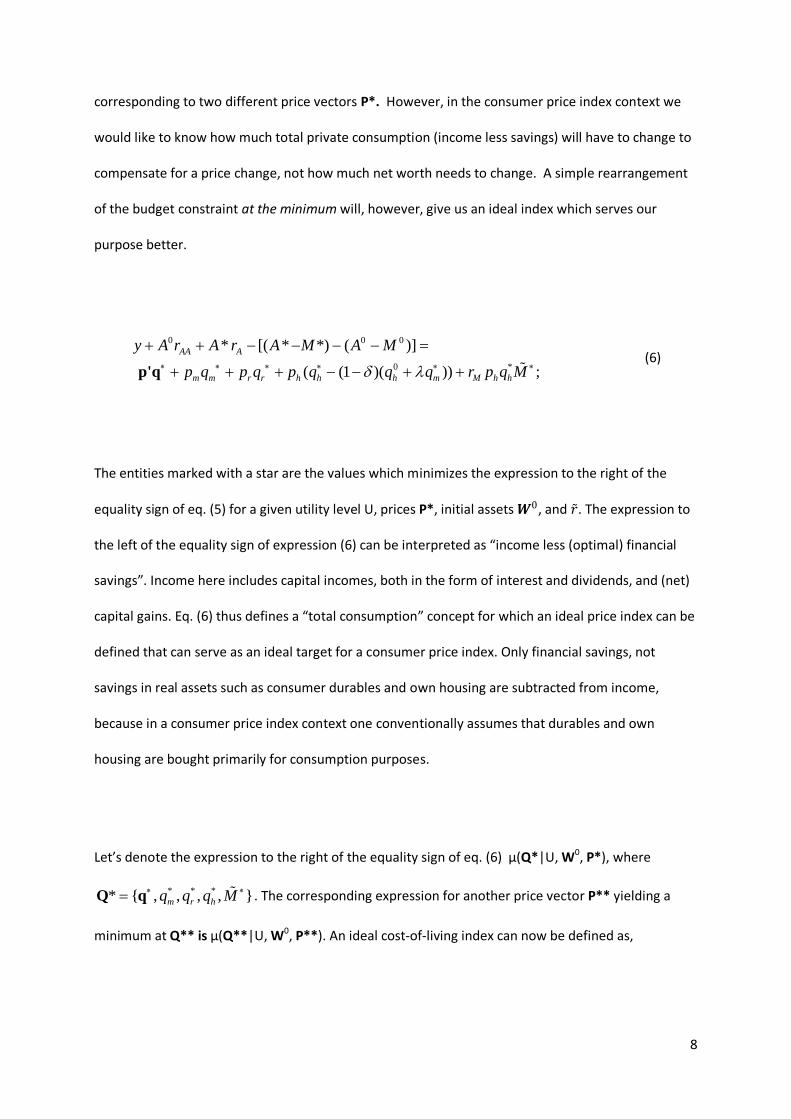
corresponding to two different price vectors P*. However, in the consumer price index context we

would like to know how much total private consumption (income less savings) will have to change to

compensate for a price change, not how much net worth needs to change. A simple rearrangement

of the budget constraint at the minimum will, however, give us an ideal index which serves our

purpose better.

0 0 0

0 *

* [( * *) ( )]

( (1 )( )) ;AA A

m m r r h h h m M h h

y A r A r A M A M

p q p q p q q q r p q Mδ λ∗ ∗ ∗ ∗ ∗ ∗

+ + − − − − =

+ + + − − + +p'q (6)

The entities marked with a star are the values which minimizes the expression to the right of the

equality sign of eq. (5) for a given utility level U, prices P*, initial assets 𝑾𝑾0, and �̃�𝑟. The expression to

the left of the equality sign of expression (6) can be interpreted as “income less (optimal) financial

savings”. Income here includes capital incomes, both in the form of interest and dividends, and (net)

capital gains. Eq. (6) thus defines a “total consumption” concept for which an ideal price index can be

defined that can serve as an ideal target for a consumer price index. Only financial savings, not

savings in real assets such as consumer durables and own housing are subtracted from income,

because in a consumer price index context one conventionally assumes that durables and own

housing are bought primarily for consumption purposes.

Let’s denote the expression to the right of the equality sign of eq. (6) μ(Q*|U, W0, P*), where

* * ** { , , , , }m r hq q q M∗ ∗=Q q . The corresponding expression for another price vector P** yielding a

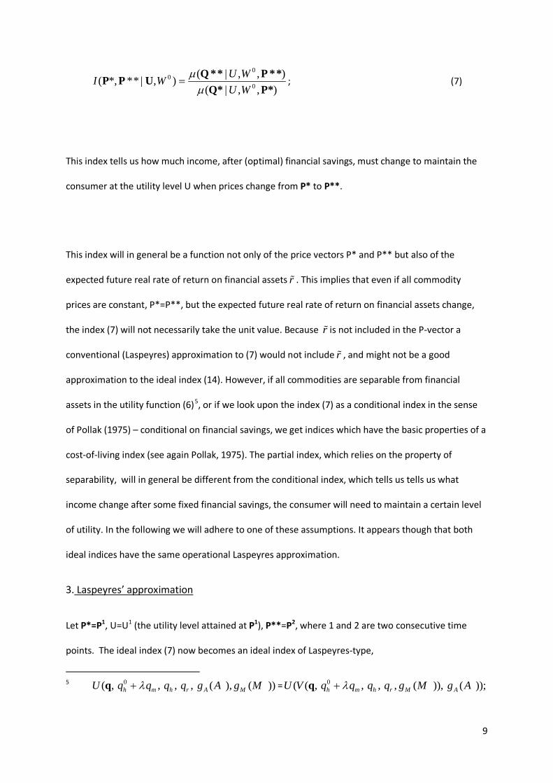
minimum at Q** is μ(Q**|U, W0, P**). An ideal cost-of-living index can now be defined as,

9

0

00

( | , , )( *, ** | , )( | , , )

U WI WU W

µµ

=Q ** P **P P U

Q* P*; (7)

This index tells us how much income, after (optimal) financial savings, must change to maintain the

consumer at the utility level U when prices change from P* to P**.

This index will in general be a function not only of the price vectors P* and P** but also of the

expected future real rate of return on financial assets r . This implies that even if all commodity

prices are constant, P*=P**, but the expected future real rate of return on financial assets change,

the index (7) will not necessarily take the unit value. Because r is not included in the P-vector a

conventional (Laspeyres) approximation to (7) would not include r , and might not be a good

approximation to the ideal index (14). However, if all commodities are separable from financial

assets in the utility function (6)5

3.

, or if we look upon the index (7) as a conditional index in the sense

of Pollak (1975) – conditional on financial savings, we get indices which have the basic properties of a

cost-of-living index (see again Pollak, 1975). The partial index, which relies on the property of

separability, will in general be different from the conditional index, which tells us tells us what

income change after some fixed financial savings, the consumer will need to maintain a certain level

of utility. In the following we will adhere to one of these assumptions. It appears though that both

ideal indices have the same operational Laspeyres approximation.

Let P*=P1, U=U1 (the utility level attained at P1), P**=P2, where 1 and 2 are two consecutive time

points. The ideal index (7) now becomes an ideal index of Laspeyres-type,

Laspeyres’ approximation

5 0( , , , , ( ), ( ))h m h r A MU q q q q g A g Mλ+q = 0( ( , , , , ( )), ( ));h m h r M AU V q q q q g M g Aλ+q

10

1 0 2

1 2 1 01 1 0 1

( | , , )( , | , )( | , , )

U WI U WU W

µµ

=Q ** PP PQ P

(8)

Q** is in general not equal to observable Q2, because Q** is an optimum conditional on U1 and W0,

while Q2 is an optimum conditional on U2 and W1. It is thus not possible to compute this index, but an

upper limit is the Laspeyres index,6

1 2

1 21 1

( | )( , )

( | )L

LL

Iµµ

=Q P

P PQ P

; (9)

Introducing three tax parameters in eq. (6) - a flat rate capital tax τ and a real estate tax 𝜏𝜏ℎ

proportional to a tax assessed value, obtained as the product of the tax parameter β and the market

value of the property – and time period top scripts, we can write the numerator of index (9) as

follows,

1 2 2 1 2 1 2 1

2 1 0 1 2 2 2 1 1 2 2 2 1

( | )

( (1 )( )) (1 )h h

L m m r r

h h h m M h h h

p q p q

p q q q r p q M p q

µ

δ λ τ τ β

= + + +

− − + + − +

Q P p 'q

; (10)

and analogously for 1 1( | )Lµ Q P . This index applies to a single consumer. Using the conventional so

called plutocratic index it can be shown that the numerator of the Lapeyres index for the whole

population of consumers can be written7

6 This property of the Laspeyers index holds if the utility function is separable or if the ideal index is a conditional index.

,

11

1 2

2 2 221 1 1 1 1 1 1 1 0 1

1 1 1 1

2 2 2 22 21 1 1 1 1 1 1

1 1 1 1 1 1

( | )

( (1 )( ))

(1 )(1 )

(1 )

Lii

j m hrj ji m mi r ri h hi hi mi

j i i i ij m r h

h h hMM i h h hi

i iM h h h

p p ppp q p q p q p q q q

p p p p

p prr M p q

r p p

µ

δ λ

τ βττ τ β

τ τ β

=

+ + + − − + +

−− +

−

∑

∑ ∑ ∑ ∑ ∑

∑ ∑

Q P

(11)

where i is the summation script for consumers and j the summation script for non-housing

commodities. The first term corresponds to a price index for non-housing commodities, the second

to an index for maintenance and repair, the third to an index for rented dwellings, the fourth to an

index for investments in new housing, the fifth represents interest payments on mortgages and the

last captures the real estate tax. Note that investments in new housing can either be done by buying

a new house or by repairing and improving an already existing house. But also note that the market

value of houses which exist in both periods will cancel out in the weight sum of the fourth index

component. This weight sum will just be the sum of the market values of new built houses less the

values of demolished houses.

The index component for interest payments has a price relative which depends on the interest rate,

the tax rate and the market price of owned dwellings. If it is not consistent with the purpose of the

index to allow for changes in the tax rates one can condition on a certain value of the tax parameter,

for instance the value of the base period. The tax parameter then drops out of the price relative,

while the weight still is the sum of all interest paid after tax. The market price of owned dwellings

comes into the price relative from the assumption that utility is a function of the mortgage share.

Increases (decreases) in the market price will ceteris paribus decrease (increase) the mortgage share

and increase (decrease) utility. The consumer will then in general adjust to this change in market

prices, for instance by increasing the mortgage and/or increasing the consumption of other

7 See Klevmarken (2009), section 5.

12

commodities. However, if the change in market price is perceived as temporary, the consumer might

not adjust at all. It might be more realistic to assume that the consumer reacts to a more stable long-

run trend in real estate prices. The mortgage share should then be defined as the ratio of all

mortgages to a weighted mean of past and current prices of the property owned8

4.

. It then follows

that the real estate price ratio in the second last term of eq. (11) is replaced by a ratio of weighted

means. The implication is that changes in the market price will not have such a large immediate

impact on this index component, and the impact is thus delayed. (See further the discussion of this

issue in section 6.)

The history of a Swedish cost-of-living index dates back to 1912, while a monthly consumer price

index as we know it today was first computed in 1954.

The current Swedish CPI

9

The theoretical basis of the Swedish CPI is the economic theory for a true cost-of-living index. The CPI

is used for many purposes, but the government has decided that computation of the compensation

which consumers need to maintain their standard of living when prices change, should be the

primary target for the Swedish CPI. This implies that the CPI is used to adjust pensions, social

allowances and other income transfers to households from the public sector. It is, however, also

At this time a distinction was made between

a short term and a long term index. The index was a monthly chain index, but the weights were kept

constant throughout a year (short term index) and only changed in the beginning of January. When

the new weights were available at the end of a year the index for the past year was recomputed

using this new information. This so called long term index was then used to link the CPI to the next

year. In 2005 a new chain index construction was introduced with full year-to-year index links

according to the superlative Walsh index formula and Laspeyres year-to-month links.

8 In practice it might be difficult to know the market price of one’s own property if it has not been put on the market. The consumer is then assumed to make an estimate based on the information he can obtain from the market for similar properties. 9 Statistics Sweden (2001). In the 1930s the so called Myrdal-Bouvin index was computed to cover the period 1830-1914.

13

used as a target by the Swedish Central bank, although the bank uses alternative indices as well

which better serve the purposes of monetary policy.

Housing represents almost 30 percent of the total weight of the CPI. About half of that comprise

rented apartments and condominiums and the other half consists of owner-occupied houses. The

subindex for rented apartments is relatively uncomplicated. It is based on a questionnaire to

landlords covering a relatively large sample of dwellings. Because heating costs, hot and cold water,

citygas etc. are typically included in the rent in Sweden, the rental subindex includes these items,

while electricity for non-heating purposes is not included, but covered separately. There is no

subindex for condominiums, but the price changes of these services are represented by the index for

rented apartments.10

The design of the subindex for owner-occupied housing (mostly single family houses) originates back

to a commission appointed in 1955 to review the principles used to compute the housing subindex.

Since then the computations have been adjusted a few times. One might say that Statistics Sweden

today uses a modified user-cost approach for owner-occupied housing, however the current model is

not theoretically derived from a user-cost model. The following items are included: mortgage

interest, depreciation (maintenance and repair), property tax, site lease fees, heating from different

sources, electricity, water and sewage and insurance. The subindex which is most interesting to us is

that for mortgage interest. It is computed as a product of two separate indices, an interest rate index

and a capital stock index.

The interest rate index weighs together changes in rates for mortgages of varying length issued by

banks and mortgage institutes. For contracts with a fixed rate for a given period the average rate

estimate is a moving average of past and present rates that apply to this kind of contract. For

10 Considering that there has been rent control in Sweden since World War II, while the market for condominiums is free and that prices of condominiums has increased about as much as prices of detached houses, at least in the big cities, it is not an ideal solution to allow the subindex for rented apartments to represent the price change in housing services from condominiums. See the comment at the end of the paper.

14

instance, for mortgages which have a fixed rate for five years, all five years fixed rates in the past 60

months are averaged. Past changes in interest rates will thus influence current inflation.

The capital stock index does not measure changes in the current market value of the stock of owner-

occupied dwellings, but rather changes in the purchase values as of the time of purchase. A house

that does not change owner contributes the same value to the numerator and denominator of the

index, this value is the price at which the house was sold when it last changed owner. A house that

was sold in the index period contributes its new price to the numerator and its old price to the

denominator. The old price might then date many years back. New built houses enter the numerator

with the purchase price and the same price, deflated to the base period by a price index for newly

built single-family houses, is used in the denominator.

The logic behind the treatment of interest in combination with the capital stock in this index

construct is not straight forward. The background is the following. The 1952 index committee

suggested that one should only include interest on borrowed capital. The National Board of Health

and Welfare wanted to include interest on both borrowed and own capital at current market values.

The 1955 commission accepted that interest should apply to both borrowed and own capital, but did

not want to use the current market values. The commission criticized the National Board of Health

and Welfare (Chapter IV, section 2b)11

11 Translated by the authors

: “In our view the less convincing arguments of The National

Board of Health and Welfare become very clear in their treatment of the cost of interest. That

increasing real estate prices through a computed increase in the wealth of house owners would give

them increased interest costs and also increased costs of living is in our view an untenable

interpretation of the concepts of cost and expenditure in the index context.” The commission instead

suggested that the cost of depreciation as well as the cost of interest should be computed against

the market value of the house at the time when the present owner once bought his house. The

commission also added (Chapter VI, section 2c): “If the cost of building a new house increases, the

15

costs of depreciation and interest increases for those who build new homes. These changes should

influence index. The same is true for the share of owned homes which change owners in a year.”

After the 1955 commission Statistics Sweden has computed a capital stock index from historical

transaction prices. The construction of this index thus implies that an increase in the market value of

a house that does not change owner does not contribute to increase the capital stock index, while a

house which does change owner contributes the price change during the whole period the seller

owned the house. The result is that changes in the market price of owner-occupied houses are

smoothed and that historical movements in the price will influence the current index link. Another

implication is that changes in the turn-over of the housing market will influence the price index.

There is no distinction between borrowed and own capital. The index aims at capturing both interest

paid and foregone. The weight thus covers both borrowed and own capital, but valued at historical

transaction prices.

The treatment of depreciation and maintenance and repair in the current CPI also needs a comment.

The weight of the depreciation index is obtained from the assumption that 1.4 percent of the total

market value of an owner-occupied home, excluding the land value, is depreciated each year. The

price component includes price measures of goods and services used to maintain and repair a house.

In addition to the depreciation index there is a subindex for minor maintenance and repair

commodities only covering material.

5.

We now return to the implementation of Klevmarken’s index. The differences between this index

and the current Swedish CPI are found in the treatment of housing, in particular in the index for

owner-occupied housing. We thus compute all non-housing items exactly as in the CPI. This also

means that we have followed the CPI design used in each period. The computations have been done

as if Klevmarken’s approach had been used for the CPI.

Choice of price measures and weight data

16

The CPI subindex for rent and the corresponding weight were used to compute Klevmarken’s index.

We also used CPI data for electricity, heating, citygas to multifamily buildings, water and sewage, and

insurance of single family housing.

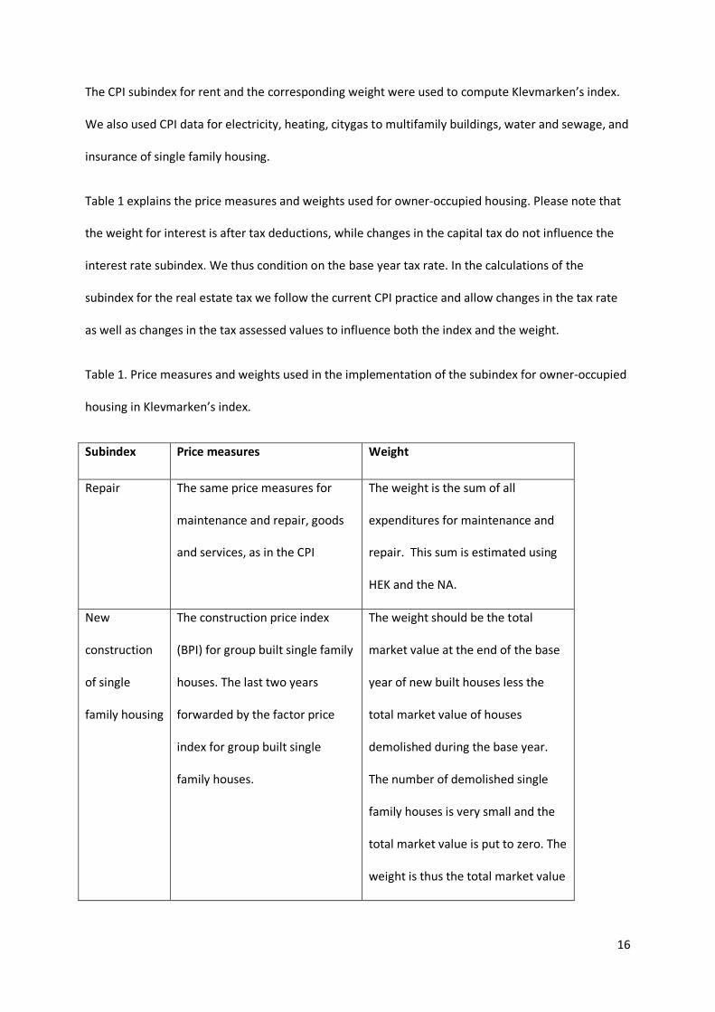
Table 1 explains the price measures and weights used for owner-occupied housing. Please note that

the weight for interest is after tax deductions, while changes in the capital tax do not influence the

interest rate subindex. We thus condition on the base year tax rate. In the calculations of the

subindex for the real estate tax we follow the current CPI practice and allow changes in the tax rate

as well as changes in the tax assessed values to influence both the index and the weight.

Table 1. Price measures and weights used in the implementation of the subindex for owner-occupied

housing in Klevmarken’s index.

Subindex Price measures Weight

Repair The same price measures for

maintenance and repair, goods

and services, as in the CPI

The weight is the sum of all

expenditures for maintenance and

repair. This sum is estimated using

HEK and the NA.

New

construction

of single

family housing

The construction price index

(BPI) for group built single family

houses. The last two years

forwarded by the factor price

index for group built single

family houses.

The weight should be the total

market value at the end of the base

year of new built houses less the

total market value of houses

demolished during the base year.

The number of demolished single

family houses is very small and the

total market value is put to zero. The

weight is thus the total market value

17

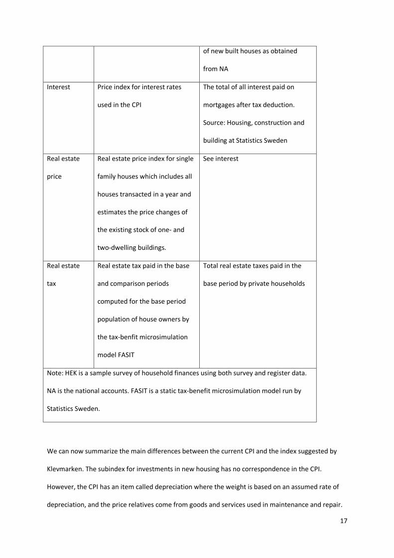
of new built houses as obtained

from NA

Interest Price index for interest rates

used in the CPI

The total of all interest paid on

mortgages after tax deduction.

Source: Housing, construction and

building at Statistics Sweden

Real estate

price

Real estate price index for single

family houses which includes all

houses transacted in a year and

estimates the price changes of

the existing stock of one- and

two-dwelling buildings.

See interest

Real estate

tax

Real estate tax paid in the base

and comparison periods

computed for the base period

population of house owners by

the tax-benfit microsimulation

model FASIT

Total real estate taxes paid in the

base period by private households

Note: HEK is a sample survey of household finances using both survey and register data.

NA is the national accounts. FASIT is a static tax-benefit microsimulation model run by

Statistics Sweden.

We can now summarize the main differences between the current CPI and the index suggested by

Klevmarken. The subindex for investments in new housing has no correspondence in the CPI.

However, the CPI has an item called depreciation where the weight is based on an assumed rate of

depreciation, and the price relatives come from goods and services used in maintenance and repair.

18

Depreciation is a theoretical concept used to capture the wear and tear of the housing stock, but it is

not part of the reality of a house owner and thus difficult to measure. The model used in Klevmarken

(2009) includes depreciation, it is implicitly part of the item for investment in new housing, but as

noted above it is netted out in the aggregation and no specific measure of depreciation is needed.

Klevmarken’s index rather includes a straight forward subindex of goods and services for

maintenance and repair.

The most important difference is found in the subindex for interest. Both the price component and

the weight differ. The weight becomes much smaller in Klevmarken’s index because it only covers

interest paid on borrowed capital after tax deduction, while in the CPI interest is computed for both

borrowed and own capital, and without tax deduction. While the interest index is identical, the way

changes in real estate prices are accounted for is quite different. As explained above the CPI uses

historical purchase values which results in a smoother index compared to the price changes in the

market. In Klevmarkens’s index changes in current market prices determine the price relatives. (See

though the discussion of alternative ways of formulating Klevmarken’s model at the end of Section 3

and below in Section 6.)

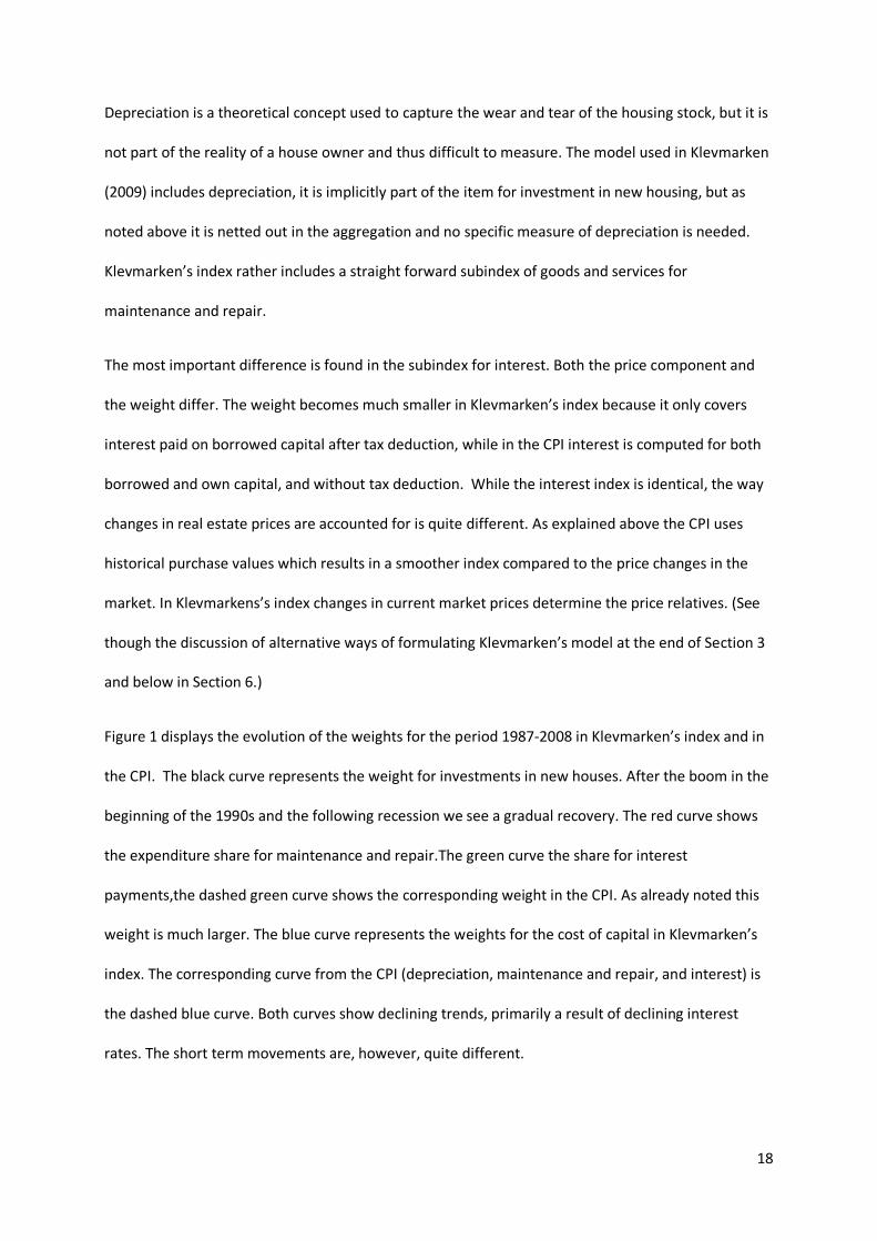
Figure 1 displays the evolution of the weights for the period 1987-2008 in Klevmarken’s index and in

the CPI. The black curve represents the weight for investments in new houses. After the boom in the

beginning of the 1990s and the following recession we see a gradual recovery. The red curve shows

the expenditure share for maintenance and repair.The green curve the share for interest

payments,the dashed green curve shows the corresponding weight in the CPI. As already noted this

weight is much larger. The blue curve represents the weights for the cost of capital in Klevmarken’s

index. The corresponding curve from the CPI (depreciation, maintenance and repair, and interest) is

the dashed blue curve. Both curves show declining trends, primarily a result of declining interest

rates. The short term movements are, however, quite different.

19

Figure 1. Relative weights of the cost of capital and its components 1987-2008 (per mille)

6.

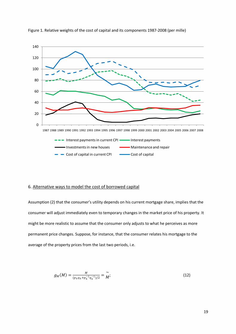
Assumption (2) that the consumer’s utility depends on his current mortgage share, implies that the

consumer will adjust immediately even to temporary changes in the market price of his property. It

might be more realistic to assume that the consumer only adjusts to what he perceives as more

permanent price changes. Suppose, for instance, that the consumer relates his mortgage to the

average of the property prices from the last two periods, i.e.

Alternative ways to model the cost of borrowed capital

𝑔𝑔𝑀𝑀(𝑀𝑀) = 𝑀𝑀(𝑝𝑝ℎ𝑞𝑞ℎ+𝑝𝑝ℎ

−1𝑞𝑞ℎ−1)/2

=~𝑀𝑀; (12)

0

20

40

60

80

100

120

140

1987 1988 1989 1990 1991 1992 1993 1994 1995 1996 1997 1998 1999 2000 2001 2002 2003 2004 2005 2006 2007 2008

Interest payments in current CPI Interest payments

Investments in new houses Maintenance and repair

Cost of capital in current CPI Cost of capital

20

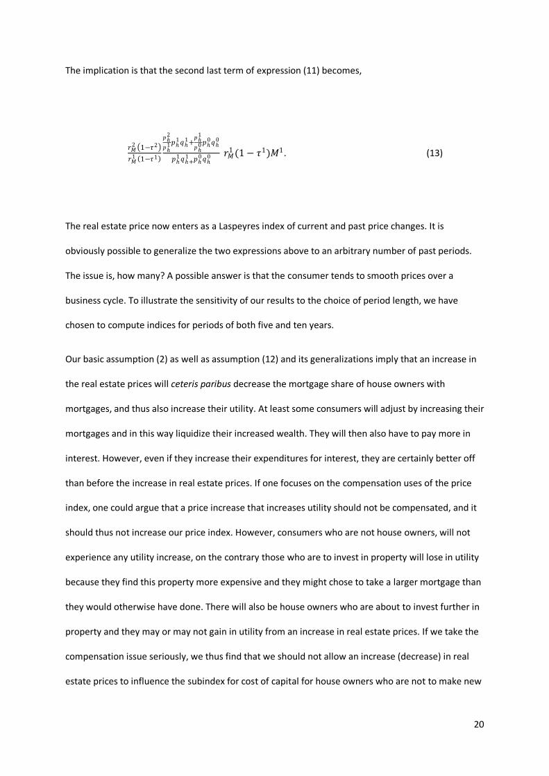
The implication is that the second last term of expression (11) becomes,

𝑟𝑟𝑀𝑀

2 �1−𝜏𝜏2�𝑟𝑟𝑀𝑀

1 (1−𝜏𝜏1)

𝑝𝑝ℎ2

𝑝𝑝ℎ1𝑝𝑝ℎ

1𝑞𝑞ℎ1+

𝑝𝑝ℎ1

𝑝𝑝ℎ0𝑝𝑝ℎ

0𝑞𝑞ℎ0

𝑝𝑝ℎ1𝑞𝑞ℎ+

1 𝑝𝑝ℎ0𝑞𝑞ℎ

0 𝑟𝑟𝑀𝑀1 (1− 𝜏𝜏1)𝑀𝑀1. (13)

The real estate price now enters as a Laspeyres index of current and past price changes. It is

obviously possible to generalize the two expressions above to an arbitrary number of past periods.

The issue is, how many? A possible answer is that the consumer tends to smooth prices over a

business cycle. To illustrate the sensitivity of our results to the choice of period length, we have

chosen to compute indices for periods of both five and ten years.

Our basic assumption (2) as well as assumption (12) and its generalizations imply that an increase in

the real estate prices will ceteris paribus decrease the mortgage share of house owners with

mortgages, and thus also increase their utility. At least some consumers will adjust by increasing their

mortgages and in this way liquidize their increased wealth. They will then also have to pay more in

interest. However, even if they increase their expenditures for interest, they are certainly better off

than before the increase in real estate prices. If one focuses on the compensation uses of the price

index, one could argue that a price increase that increases utility should not be compensated, and it

should thus not increase our price index. However, consumers who are not house owners, will not

experience any utility increase, on the contrary those who are to invest in property will lose in utility

because they find this property more expensive and they might chose to take a larger mortgage than

they would otherwise have done. There will also be house owners who are about to invest further in

property and they may or may not gain in utility from an increase in real estate prices. If we take the

compensation issue seriously, we thus find that we should not allow an increase (decrease) in real

estate prices to influence the subindex for cost of capital for house owners who are not to make new

21

investments, while it should for the share of consumers who are to invest in property in the period.

In practice it might become difficult to distinguish these groups of consumers. However, if we use a

Laspeyres approximation those who do not have any mortgage will not contribute to the subindex

for cost of capital, because in a Laspeyres index the weight is proportional to the base period

mortgage. In this case the issue then becomes how one can distinguish between those mortgage

holders who get a net gain in utility and those who get a net loss.

The compensation issue is primarily a policy issue for the index provider and not a theoretical

problem. To illustrate the numerical consequences of focusing on the compensation uses of the price

index we have computed an alternative which conditions on the base period real estate price in the

sub index for cost of borrowed capital. The change in the real estate price then drops out of this

subindex (c f the second last term of expression (11)), and it becomes a simple interest rate index.

We now have four alternative ways to implement a subindex for the cost of capital: Alternative A

conditions on the base period real estate price and is a simple interest rate index, B is our basic

model alternative in which the interest index is multiplied with an index for the change in the real

estate prices between the base and comparison periods, and D5 and D10 which are similar to B but

assume that the consumer bases its decisions on a trend in the real estate prices rather than on the

current changes. D5 has a price index of real estate prices based on the last five years of price

information, while D10 uses the last 10 years. For the period 1987-2008 Figure 2 displays these four

alternatives as well as the corresponding subindex in the current CPI.

Not unexpectedly we find that alternative A distinguishes itself from the other alternatives as it only

depends on changes in the interest rates, a trend wise decline. The three alternatives including a

property price index all group together in a much higher index path reflecting the general increase in

real estate prices. But they differ in their short term behavior. The longer moving average used in the

real estate price index, the smoother subindex we get. The current CPI subindex lies in between A

and the other alternatives, in this case the rapid increases in real estate prices at the end of the

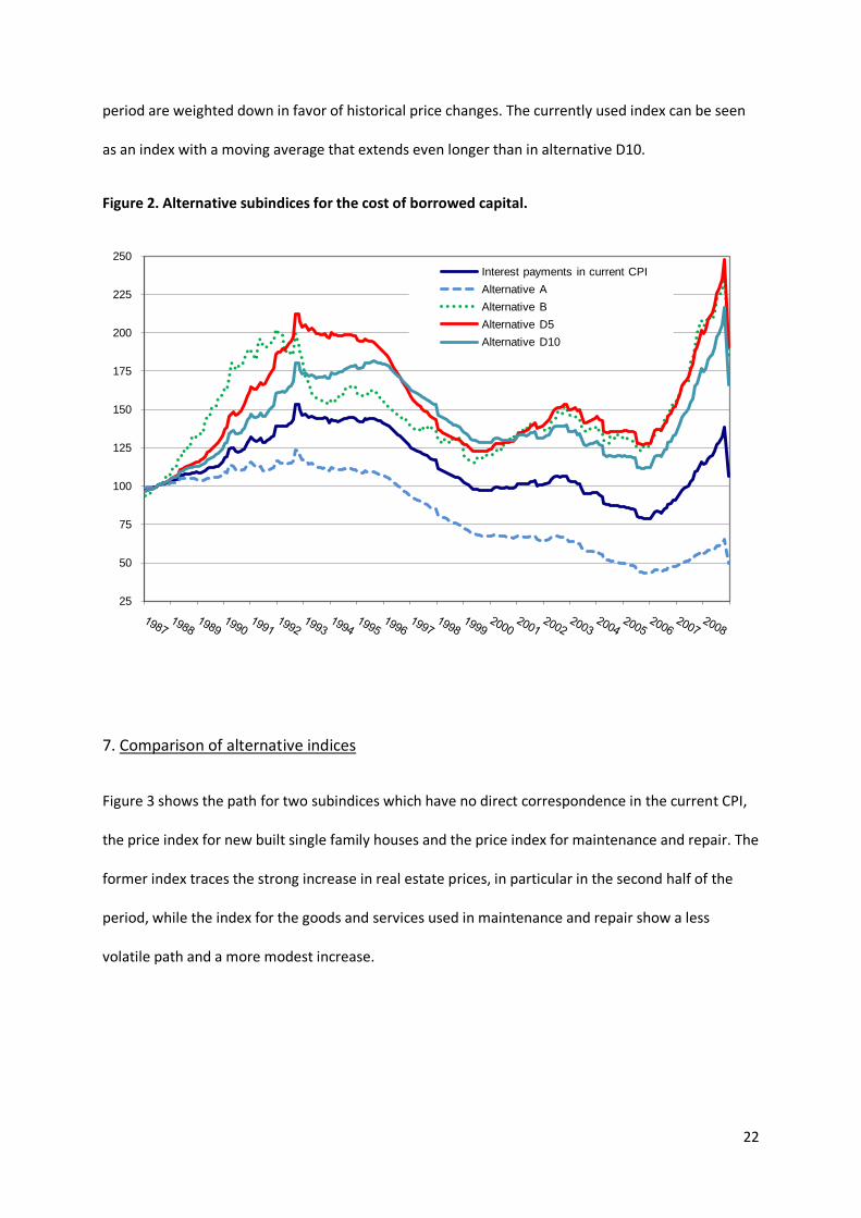
22

period are weighted down in favor of historical price changes. The currently used index can be seen

as an index with a moving average that extends even longer than in alternative D10.

Figure 2. Alternative subindices for the cost of borrowed capital.

7.

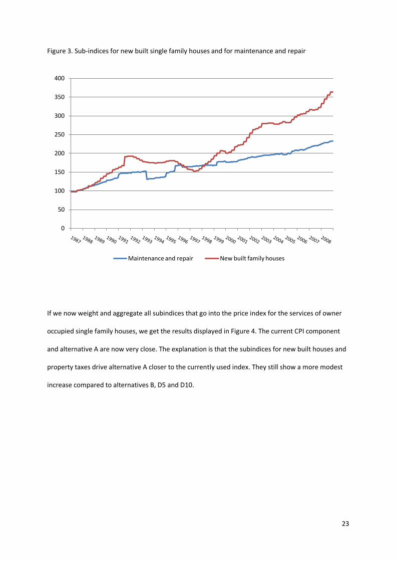
Figure 3 shows the path for two subindices which have no direct correspondence in the current CPI,

the price index for new built single family houses and the price index for maintenance and repair. The

former index traces the strong increase in real estate prices, in particular in the second half of the

period, while the index for the goods and services used in maintenance and repair show a less

volatile path and a more modest increase.

Comparison of alternative indices

25

50

75

100

125

150

175

200

225

250Interest payments in current CPIAlternative AAlternative BAlternative D5Alternative D10

23

Figure 3. Sub-indices for new built single family houses and for maintenance and repair

If we now weight and aggregate all subindices that go into the price index for the services of owner

occupied single family houses, we get the results displayed in Figure 4. The current CPI component

and alternative A are now very close. The explanation is that the subindices for new built houses and

property taxes drive alternative A closer to the currently used index. They still show a more modest

increase compared to alternatives B, D5 and D10.

0

50

100

150

200

250

300

350

400

Maintenance and repair New built family houses

24

Figure 4. Alternative indices for the price of the services from an owner occupied home 1987-2008

We can also compare the alternatives at the level of total CPI. The results are displayed in Figure 5

and Table 2. All alternatives are now much closer as all commodities but owner occupied homes are

identical. There is still, however, a clear difference between the current CPI and alternative A on one

side and B, D5 and D10 on the other. The latter increased by almost ten percentage units more than

the current CPI and alternative A from 1987 to 2008. Table 2 also gives the corresponding estimates

of the average annual rate of inflation and its standard deviation. The current CPI and alternative A

had a mean inflation rate of 2.9 percent while alternatives B, D5 and D10 had a rate of about 3.1.

The standard deviation is about 3 in all cases. Alternative A comes out as the least volatile alternative

as it is least dependent on volatile real estate prices.

50

100

150

200

250

300Owner occupied housing in current CPI

Alternative A

Alternative B

Alternative D5

Alternative D10

25

Figure 5. Alternative consumer price indices 1987-2008, base year 1987=100

Table 2. Inflation rates and corresponding standard errors from alternative consumer price indices

(%)

Statistic Current CPI Alternative A Alternative B Alternative

D5

Alternative

D10

Mean 2.88 2.88 3.11 3.08 3.07

Std. 2.94 2.86 3.05 3.09 2.99

Index Dec.

2008

(1987=100)

179.1 179.8 188.5 187.4 186.9

90,00

110,00

130,00

150,00

170,00

190,00

Current CPI

Alternative A

Alternative B

Alternative D5

Alternative D10

26

8.

Even if the average differences between the alternative indices we have analyzed might appear small

at the level of a total CPI, annual deviations are certainly large enough to become important both for

compensation purposes and in the financial markets. We thus need criteria to choose between these

alternatives. All can be accommodated within the model structure we have chosen, so the problem is

not theoretical, but rather one related to the uses of the CPI index.

Conclusions

It is interesting to note that the currently used CPI is so close to alternative A. The current index

formula can be seen as an attempt by Statistics Sweden to meet the criticism of an index that gives

compensation to consumers that become wealthier from increased real estate prices, but at the

same time recognize that increasing real estate prices will eventually drive people to increase their

mortgages and interest payments. We introduced alternative A just to avoid compensating

consumers who increased their housing wealth. If the index provider decides to focus on the

compensation uses of the CPI one should choose alternative A or an alternative which is close to A.

As discussed above, all home owners might not get a net gain in utility from an increase in the real

estate prices.

However, if the compensation issues are considered less important, and one wants an index that

approximates a true cost-of-living index , one of the alternatives B, D5 or D10 should be preferred.

For long-term price comparisons it does not seem to matter much which of these alternatives is

chosen, but in short-term comparisons it becomes important how much one smoothes the influence

of variations in real estate prices. We have argued that consumers do not necessarily react

immediately to price changes in the real estate market, but try to estimate what they think will

become more permanent changes in the price level. This justifies some smoothing, but hardly a time

span as long as a decade. The preferred choice should then be an index close to D5.

27

The theoretical discussion above and the numerical illustrations have focused on owner occupied

housing. In principle one can treat the price of services from condominiums and related forms of

housing in the same way. If data are available one can also extend the analysis to cover major

durables, and treat them as durables rather than non-durables as in the current CPI practice.

Bostadsposten i konsumentprisindex. 1955 års bostadsindexutrednings betänkande, del I. Stockholm

1955 (Report from the 1955 Housing Index Commission.)

References

Grünewald O., Lundin O. & Allansson H. (2009), Nybygge I KPI – Operationalisering av den

semidynamiska egnahemsansatsen, Memo to the Standing Committee for the Swedish CPI 2009-05-

08, Statistics Sweden, Stockholm

Klevmarken, N.A. (2009), Towards an applicable true cost-of-living index that incorporates housing,

Journal of Economic and Social Measurement, 34(1), 19-34

Konüs, A. A. (1924, 1939), The problem of the true index of the cost-of-living (in Russian), The

Economic Bulletin of the Institute of Economic Conjuncture, No 9-10, pp 64-71; English translation

1939 in Econometrica 7 (1939), 10-29

Pollak, R. A. (1975), Subindexes in the Cost-of-Living Index, International Economic Review 16(1), 135-

150

Statistics Sweden (2001), The Swedish Consumer Price Index. A handbook of methods, Örebro 2001,

ISBN 91-618-1097-5

WORKING PAPERS* Editor: Nils Gottfries 2008:1 Mikael Carlsson, Johan Lyhagen and Pär Österholm, Testing for Purchasing

Power Parity in Cointegrated Panels. 20pp. 2008:2 Che-Yuan Liang, Collective Lobbying in Politics: Theory and Empirical

Evidence from Sweden. 37pp. 2008:3 Spencer Dale, Athanasios Orphanides and Pär Österholm, Imperfect Central

Bank Communication: Information versus Distraction. 33pp. 2008:4 Matz Dahlberg and Eva Mörk, Is there an election cycle in public

employment? Separating time effects from election year effects. 29pp. 2008:5 Ranjula Bali Swain and Adel Varghese, Does Self Help Group Participation

Lead to Asset Creation. 25pp. 2008:6 Niklas Bengtsson, Do Protestant Aid Organizations Aid Protestants Only?

28pp. 2008:7 Mikael Elinder, Henrik Jordahl and Panu Poutvaara, Selfish and Prospective

Theory and Evidence of Pocketbook Voting. 31pp. 2008:8 Erik Glans, The effect of changes in the replacement rate on partial

retirement in Sweden. 30pp. 2008:9 Erik Glans, Retirement patterns during the Swedish pension reform. 44pp. 2008:10 Stefan Eriksson and Jonas Lageström, The Labor Market Consequences of

Gender Differences in Job Search. 16pp. 2008:11 Ranjula Bali Swain and Fan Yang Wallentin, Economic or Non-Economic

Factors – What Empowers Women?. 34pp. 2008:12 Matz Dahlberg, Heléne Lundqvist and Eva Mörk, Intergovernmental Grants

and Bureaucratic Power. 34pp. 2008:13 Matz Dahlberg, Kajsa Johansson and Eva Mörk, On mandatory activation of

welfare receivers. 39pp. 2008:14 Magnus Gustavsson, A Longitudinal Analysis of Within-Education-Group

Earnings Inequality. 26pp. 2008:15 Henrique S. Basso, Delegation, Time Inconsistency and Sustainable

Equilibrium. 24pp. 2008:16 Sören Blomquist and Håkan Selin, Hourly Wage Rate and Taxable Labor

Income Responsiveness to Changes in Marginal Tax Rates. 31 pp. * A list of papers in this series from earlier years will be sent on request by the department.

2008:17 Jie Chen and Aiyong Zhu, The relationship between housing investment and

economic growth in China：A panel analysis using quarterly provincial data. 26pp.

2009:1 Per Engström, Patrik Hesselius and Bertil Holmlund, Vacancy Referrals, Job

Search, and the Duration of Unemployment: A Randomized Experiment. 25 pp.

2009:2 Chuan-Zhong Li and Gunnar Isacsson, Valuing urban accessibility and air

quality in Sweden: A regional welfare analysis. 24pp. 2009:3 Luca Micheletto, Optimal nonlinear redistributive taxation and public good

provision in an economy with Veblen effects. 26 pp. 2009:4 Håkan Selin, The Rise in Female Employment and the Role of Tax

Incentives. An Empirical Analysis of the Swedish Individual Tax Reform of 1971. 38 pp.

2009:5 Lars M. Johansson and Jan Pettersson, Tied Aid, Trade-Facilitating Aid or

Trade-Diverting Aid? 47pp.

2009:6 Håkan Selin, Marginal tax rates and tax-favoured pension savings of the self-employed Evidence from Sweden. 32pp.

2009:7 Tobias Lindhe and Jan Södersten, Dividend taxation, share repurchases and

the equity trap. 27pp. 2009:8 Che-Yuan Liang, Nonparametric Structural Estimation of Labor Supply in

the Presence of Censoring. 48pp. 2009:9 Bertil Holmlund, Incentives in Business and Academia. 12pp. 2009:10 Jakob Winstrand, The Effects of a Refinery on Property Values – The Case

of Sweden. 27pp. 2009:11 Ranjula Bali Swain and Adel Varghese. The Impact of Skill Development

and Human Capital Training on Self Help Groups. 28pp. 2009:12 Mikael Elinder. Correcting Mistakes: Cognitive Dissonance and Political

Attitudes in Sweden and the United States. 25 pp. 2009:13 Sören Blomquist, Vidar Christiansen and Luca Micheletto: Public Provision

of Private Goods and Nondistortionary Marginal Tax Rates: Some further Results. 41pp.

2009:14 Mattias Nordin: The effect of information on voting behavior. 34pp. See also working papers published by the Office of Labour Market Policy Evaluation http://www.ifau.se/ ISSN 1653-6975