Coastal Engineering 67 (2012) 54–66

Contents lists available at SciVerse ScienceDirect

Coastal Engineering

j ourna l homepage: www.e lsev ie r .com/ locate /coasta leng

A new approach to handle wave breaking in fully non-linear Boussinesq models

M. Tissier a,⁎, P. Bonneton a, F. Marche b, F. Chazel c, D. Lannes d

a Université Bordeaux 1, CNRS, UMR 5805-EPOC, Talence, F-33405, Franceb I3M, Université de Montpellier 2, CC 051, F-34000, Montpellier, Francec Université de Toulouse, UPS/INSA, IMT, CNRS UMR 5219, F-31077 Toulouse, Franced DMA, Ecole Normale Supérieure et CNRS UMR 8553, 45 rue d'Ulm, F-75005, Paris, France

⁎ Corresponding author. Now at Institute for Marine apartment of Physical Geography, Faculty of Geoscience80115, 3508 TC, Utrecht, The Netherlands. Tel.: +31 353 11 45.

E-mail addresses: M.F.S.Tissier@uu.nl (M. Tissier),p.bonneton@epoc.u-bordeaux1.fr (P. Bonneton), fabien.(F. Marche), florent.chazel@math.univ-toulouse.fr (F. Ch(D. Lannes).

0378-3839/$ – see front matter © 2012 Elsevier B.V. Alldoi:10.1016/j.coastaleng.2012.04.004

a b s t r a c t

a r t i c l e i n f o

Article history:Received 16 November 2011Received in revised form 9 April 2012Accepted 11 April 2012Available online 14 May 2012

Keywords:Finite volumeBreaking modelShock theoryFully non-linear Boussinesq model

In this paper, a newmethod to handle wave breaking in fully non-linear Boussinesq-typemodels is presented.The strategy developed to treat wave breaking is based on a reformulation of the set of governing equations(namely Serre Green–Naghdi equations) that allows us to split them into a hyperbolic part in the conservativeform and a dispersive part. When a wave is ready to break, we switch locally from Serre Green–Naghdi equa-tions to Non-linear Shallow Water equations by suppressing the dispersive terms in the vicinity of the wavefront. Thus, the breaking wave front is handled as a shock by the Non-linear Shallow Water equations, and itsenergy dissipation is implicitly evaluated from the mathematical shock-wave theory. A simple methodology tocharacterize the wave fronts at each time step is first described, as well as appropriate criteria for the initiationand termination of breaking. Extensive validations using laboratory data are then presented, demonstratingthe efficiency of our simple treatment for wave breaking.

© 2012 Elsevier B.V. All rights reserved.

1. Introduction

Non-linear wave transformations in shallow water, and associatedprocesses such as wave-breaking and run-up, play a key role in thenearshore dynamics. A detailed knowledge of instantaneous non-linear wave characteristics is required in place of wave-averagedquantities for an accurate prediction of suspended sediment transport.Elgar et al. (2001) highlighted the importance of wave asymmetry foronshore bar migration, while recent studies focused on the influenceof different combinations of wave skewness and asymmetry on thenet sediment flux (Grasso et al., 2011; Ruessink et al., 2009). Non-linear effects are also responsible for the generation of infra-gravitywaves, which can strongly affect beach and dune erosion duringhigh energy events (Roelvink et al., 2009). An accurate descriptionof non-linear wave transformations is also necessary for the studyof coastal flooding due to storm waves or tsunamis. The descriptionof these highly non-linear and unsteady processes requires phase-resolving models with a good description of breaking and run-upover complex bathymetries. Themost accuratemodels for the descrip-tion of wave breaking are based on the Navier–Stokes equations. They

nd Atmospheric Research, De-s, Utrecht University, P.O. Box02 53 74 53; fax: +31 3 02

marche@math.univ-montp2.frazel), david.lannes@ens.fr

rights reserved.

can give a detailed description of wave breaking, including waveoverturning, but are highly computationally demanding and thereforenot suitable for large scale propagation applications. For this reason,phase-resolving models based on depth-averaged equations are stillan attractive way to describe wave transformation in the nearshorezone. Two kinds of approaches can be considered: the models can bebased on Non-linear Shallow Water (NSW) or Boussinesq-type (BT)equations.

NSWmodels, with the help of shock-capturing schemes, can accu-rately reproduce broken wave dissipation and swash oscillationswithout any ad hoc parametrization (Bonneton, 2007; Brocchini andDodd, 2008; Kobayashi et al., 1989; Marche et al., 2007). The absenceof dispersive effects restricts their validity domain to areaswhere non-linearities predominate, such as the inner surf and swash zones. Theyare in particular not valid in the shoaling zone, since the absence ofdispersive effects would lead to an incorrect prediction of the locationof wave breaking. On the other hand, BT equations take into account atdifferent degrees of accuracy both non-linear and dispersive aspects ofwave propagation. Denoting by a the order of free‐surface amplitude,h0 the characteristic water depth and L the characteristic horizontalscale, most of Boussinesq models used for nearshore applications arebased on a classical shallow water assumption μ=(h0/L)2≪1 and bal-ance between dispersion and non-linearity ε=O(μ)≪1,with ε=a/h0.Yet, these assumptions do not always hold in the nearshore, in particu-lar in the final stages of shoaling and in the surf and swash zones, whereε can be of order 1. For such applications, fully non-linear BT equationsare required. Wei et al. (1995) showed that accounting for strong non-linearities in BT approaches leads to significantly improved predictions

55M. Tissier et al. / Coastal Engineering 67 (2012) 54–66

of wave heights, wave celerities and internal kinematics priorto breaking. The first set of fully non-linear BT equations was derivedby Serre (1953), and extended to the 2D case by Green and Naghdi(1976). These equations, called Serre Green–Naghdi (S–GN) equationsthereafter, are now recognized to be the relevant system to describefully non-linear weakly dispersive waves propagating in the nearshore(Lannes and Bonneton, 2009). They can accurately predict most phe-nomena exhibited by non-breaking waves in finite depth. However,as they do not include intrinsically energy dissipation due to wavebreaking, they become invalid in the surf zone. Besides, S–GNdispersiveterms become nonphysical in the vicinity of the breaking wave fronts.Several attempts have been made to introduce wave breaking in BTmodels by the mean of ad hoc techniques (e.g., Cienfuegos et al., 2010;Kennedy et al., 2000; Madsen et al., 1997). These approaches generallyrequire (1) the inclusion of an energy dissipation mechanism throughthe activation of extra terms in the governing equations when wavebreaking is likely to occur; (2) explicit criteria to activate/deactivatethese extra terms; (3) a method to follow the waves during theirpropagation since the breaking parametrizations depend on the ageof the breaker. Moreover, the breaking model parameters need to becalibrated to ensure that the artificially induced energy dissipation isin agreement with the rate of energy dissipated in surf zone waves.FUNWAVE (Kirby et al., 1998) is a well-known example of this kind ofmodels. It is based on the fully non linear Boussinesq equations of Weiet al. (1995),with additional parametrizations to includewave breakingand run-up (Kennedy et al., 2000). Except for being formulated in termsof the velocity vector at an arbitrary z level, the equations of Wei et al.are equivalent to the S–GN equations.1 FUNWAVE gives a very gooddescription of wave transformations in the nearshore, but each useof the model implies the tuning of several parameters, as the ones de-termining wave‐breaking dissipation and run-up (Bruno et al., 2009).Recently, Cienfuegos et al. (2010) showed that Kennedy et al.'s eddyviscosity breaking model could hardly predict simultaneously accuratewave height and asymmetry along the surf zone. This observation mo-tivated the development of a new 1D wave-breaking parametrizationincluding viscous-like effects on both the mass and the momentumequations. This approach is able to reproduce wave height decayand intraphase non-linear properties within the entire surf zone(Cienfuegos et al., 2010). However, the extension of this parametriza-tion to 2Dwave cases remains a very difficult task. Therefore, alternativeapproaches to handle wave breaking in BT models may prove veryuseful.

Recently, the so-called non-hydrostatic models, governed by theNSW equations including non-hydrostatic pressure, have been intro-duced as an alternative to BT models2 (e.g., Zijlema et al., 2011). Theycan be run in multi-layered mode, improving their frequency

1 It is shown in Lannes and Bonneton (2009) that the Green–Naghdi Eqs. (1) and (2)are the same, written in a different form, as the equations derived in Green and Naghdi(1976) and Miles and Salmon (1985). In Wei et al. (1995), the velocity unknown is notthe averaged velocity u but, as in Nwogu (1993), the velocity taken at one arbitrarydepth zα (t, x), denoted by Vα (t, x)=V (t, x, zα (t, x)). Replacing u in (1)–(2) by its ex-pression in terms of Vα yields the same equations as in Wei et al. (1995), up to O(μ2)terms. We refer to Section 2 of Chazel et al. (2010) for more details on this point.

2 However, the model derived in Zijlema et al. (2011) in its one-layer formulation(Eqs. (18)–(21)) can be rewritten in a quasi BT form:

∂tζ þ ∂x huð Þ ¼ 0

∂tuþ u∂xuþ g∂xζ ¼ 14h

∂x h3∂xtu� �

−∂x h2∂x huð Þ∂xu� �h i

;

where several non-linear terms present in the S–GN equations have been neglected;moreover, the linear wave celerity associated to these equations is given by c2=gh0

(1−μ/4) which differs at order O(μ) from the exact linear wave celerity c2 ¼ gh0tanh μ1=2ð Þ

μ1=2 ,

while for standard Boussinesq models one gets c2=gh0 (1−μ/3+O(μ2)), which iscorrect up to O(μ2) terms. The precision of these models, that is, the error betweenthe solution of the Green–Naghdi equations and the solution of the full Euler equa-tions is then of order O(μ2t), as shown in Alvarez-Samaniego and Lannes (2008).

dispersion properties, but also include a special treatment for wavebreaking (classical Prandlt mixing length parametrization) as theydo not explicitly account for small-scale turbulent processes.

The fully non-linear numerical model presented in this study isbased on S–GN equations. It is worthwhile to note that S–GN equa-tions degenerate naturally into NSW equations when dispersiveeffects are negligible. These equations are therefore well-suited to de-scribe wave propagation until the swash zone. In order to treat wavebreaking, a hybrid approach has been developed. S–GN equationsare reformulated in away that allows us to split them into a hyperbolicpart corresponding to the NSW equations in the conservative formand a dispersive part (see Bonneton et al., 2011b). The idea is to switchfrom S–GN to NSW equations when the wave is ready to break bysuppressing the dispersive term. This method allows for a naturaltreatment of wave breaking, since the energy dissipation due to wavebreaking is predicted implicitly by the shock theory, and does notrequire to be parametrized. It is an important point since the amountof energy dissipated will determine crucial phenomena such as thewater level set-up (Bonneton, 2007), and will impact wave-driven cir-culation (Bonneton et al., 2010; Bühler, 2000; Smith, 2006).

From a numerical point of view, an operator-splitting approachwithhybrid finite volume/finite‐difference schemes has been implemented(Bonneton et al., 2011b), allowing for the most effective schemes tobe used for each part of the equations. Some hybrid numerical methodshave already been developed in the past years, mainly within theframework of weakly non-linear BT equations (Briganti et al., 2004;Erduran, 2007; Erduran et al., 2005; Orszaghova et al., 2012; Shiachand Mingham, 2009; Soares-Frazão and Guinot, 2008; Soares-Frazãoand Zech, 2002; Tonelli and Petti, 2009, 2010, 2012; Weston et al.,2003), but also recently within the framework of fully-non‐linear BTmodels (Shi et al., 2012). Among thesemodels, only few take advantageof the shock-capturing properties of the Finite Volume schemes to treatwave breaking (Orszaghova et al., 2012; Shi et al., 2012; Tonelli andPetti, 2009, 2010, 2012;Weston et al., 2003). A natural approach to han-dle wave breaking with this kind of models is to estimate the breakingpoint location and subsequently divide the numerical domain spatiallyinto pre- and post- breaking areas, respectively governed by BT andNSW equations (e.g. Shi et al., 2012; Tonelli and Petti, 2009, 2010;Weston et al., 2003). This simple decomposition is of great interest forengineering purposes, in particular for the study of submersion risks,traditionally based on NSW models. Indeed, it allows for an accurateand simple description of both non-breaking and breaking wave trans-formations, and a treatment of shoreline motions without any parame-trization. However, most of these models do not include an explicitcriterion for the termination of breaking. Applying these methods tothe description of irregular wave trains propagating over uneven ba-thymetries is therefore not straightforward, since in this case, series ofalternatively breaking and non-breaking waves can be observed at agiven time. It is only recently that Tonelli and Petti (2012) appliedan extended version of their hybrid model (including an additionalcriterion for the switch back to BT equations) to describe the transfor-mation of irregular waves.

In this paper, a new approach to handle wave breaking in hybridmodels is presented. Instead of defining extended breaking areaswhere theflow is governed by theNSWequations, we treat individuallythe breaking of each wave front. More precisely, our breaking modelis based on switches performed locally in space and time from S–GNto NSW equations in the vicinity of the wave fronts. With this localtreatment, we intend to obtain a model able to account simultaneouslyand accurately for the effects of dispersion, non-linearities and wavebreaking for a given wave. This is of importance when consideringfor instance tsunami wave front transformations in the nearshore,which can evolve into a large range of bore types, including partiallybreaking undular bores. Moreover, the proposed "wave-by-wave"treatment allows for a precise description of the breaking events,from the initiation to the termination. The approach is therefore

56 M. Tissier et al. / Coastal Engineering 67 (2012) 54–66

well-suited to describe the transformation of irregular wave trains, aswell as their transformations over complex bathymetries, includingbarred beaches.

The numerical model is briefly described in Section 2. The strategydeveloped to handle wave breaking is then presented in Section 3.Extensive validations using experimental data are then performed(Section 4), including periodic wave transformations over a planarbeach, solitary wave breaking, run-up and overtopping, and wavebreaking over a bar. At last, some preliminary tests concerning hydraulicbore dynamics are performed, showing promising results concerningthe model ability to predict the complex transition from undular tobreaking bore.

2. Description of the model

Our model is based on a new 2D conservative S–GN formulation.These equations and the numerical methods to solve them are de-scribed in Bonneton et al. (2011b). In this section we sum up themain characteristics of our S–GN model in 1D.

2.1. Governing equations

The model is based on the S–GN equations. These equations can beformulated in term of the conservative variables (h, hu) in the followingdimensionalized form:

∂thþ ∂x huð Þ ¼ 0;

∂t huð Þ þ ∂x hu2 þ gh2=2� �

¼ −gh∂xbþD−f1h

uk ku;

8<: ð1Þ

with u the depth‐averaged horizontal velocity, ζ the surface elevation, hthe water depth, b the variation of the bottom topography and f a non-dimensional friction coefficient. D characterizes non-hydrostatic anddispersive effects and writes:

D ¼ 1αgh∂xζ− 1þ αhT 1

h

� �−1 1αgh∂xζ þ hQ1 uð Þ

� �; ð2Þ

where the linear operator T is defined as

T w ¼ −h2

3∂2x w−h∂xh∂xwþ ∂xζ∂xbþ h

2∂2x b

� �w; ð3Þ

and:

Q1 uð Þ ¼ 2h∂x hþ b2

� �∂xuð Þ2 þ 4

3h2∂xu∂

2x uþ h∂2

x bu∂xu

þ ∂xζ∂2x bþ h

2∂3x b

� �u2

: ð4Þ

α is an optimization parameter that should be taken equal to 1.159 inorder to minimize the phase and group velocity errors in comparisonwith the linear Stokes theory (see the dispersion correctionmethod dis-cussed in Cienfuegos et al. (2006)). Note that the range of validity of thisset of equations can been extended to deeper water, using some addi-tional optimization parameters, as described in Chazel et al. (2010).

The proposed formulation has two important advantages. Firstof all, the dispersive term does not require the direct computationof any third order derivative, allowing for more robust numericalcomputations. Moreover, if D=0, we obtain the NSW equations intheir conservative form. The formulation is therefore well-suited fora splitting approach separating the hyperbolic and the dispersivepart of the equations, allowing for an easy coupling of the sets ofequations.

2.2. Numerical methods

At each time step δt, we decompose the solution operator S(·) as-sociated to Eq. (1) by the second order splitting scheme

S δtð Þ ¼ S1 δt=2ð ÞS2 δtð ÞS1 δt=2ð Þ; ð5Þ

where S1 and S2 are respectively associated to the hyperbolic and dis-persive parts of the S–GN Eq. (1). More precisely:

• S1 (t) is the solution operator associated to NSW equations

∂thþ ∂x huð Þ ¼ 0;

∂t huð Þ þ ∂x hu2 þ gh2=2� �

¼ −gh∂xb−f1h∥u∥u:

8<: ð6Þ

• S2 (t) is the solution operator associated to the remaining (dispersive)part of the equations,

∂th ¼ 0;∂t huð Þ ¼ D:

�ð7Þ

2.2.1. Hyperbolic partOur S–GNmodel has been developed as an extension of the widely

validated NSW code SURF-WB (see Berthon and Marche, 2008;Marche et al., 2007). The system (6) can be regarded as a hyperbolicsystem of conservation laws with a topography source term and afriction term. To perform numerical approximations of the weaksolutions of this system, we use high‐order finite volume method inconservative variables, based on a positive preserving relaxationscheme and MUSCL reconstructions (see Berthon and Marche(2008)). Since we aim at computing the complex interactions be-tween propagating waves and topography, including the preservationof motionless steady states, a well-balanced scheme is used for thediscretization of the topography source term (see Audusse et al.,2004). Gathering these approaches, we obtain a high-order positivepreserving well-balanced shock-capturing scheme, able to handlebreaking bores propagation as well as moving shorelines withoutany trackingmethod (Marche et al., 2007). The friction term is treatedfollowing the method presented in Berthon et al. (2011).

2.2.2. Dispersive termsSystem (7) is solved at each time step using a classic fourth-order

finite-difference approach. It is worth mentioning that we only needto solve one scalar equation (rather than a set of two equations)during this dispersive step. Indeed, h remains constant owing to thefirst equation of (7).

Concerning the time discretization, explicit methods are used bothin (S1) and (S2). The systems are integrated in time using a classicalfourth-order Runge–Kutta method.

2.2.3. Treatment of the shorelineNo special tracking procedure is used to handle shoreline motions.

Dry cells are defined as those in which the water depth is less than athreshold value hε. A small routine is applied to ensure the stabilityof the numerical results at the shoreline: when the water depth h issmaller than hε, we impose v=0 (hε=10−5 in Section 4). The disper-sive terms are suppressed when the water depth vanishes.

Extensive validations of the numerical methods for the 1D problemcan be found in Bonneton et al. (2011a,b) and Chazel et al. (2010).

3. Wave breaking

Prior to breaking, S–GN equations give a very accurate descriptionof wave transformations, including internal kinematics (Carter andCienfuegos, 2011). However, depth-averaged approaches cannot

57M. Tissier et al. / Coastal Engineering 67 (2012) 54–66

reproduce wave overturning and small-scale processes related towave breaking. Approximate representations of the breaking process-es are therefore needed. They are generally less accurate in the firststages of breaking, in particular for plunging breakers. By switchinglocally to NSW equations, we decide to represent breaking wavefronts as shocks: we conserve mass and momentum across the wavefront, and allow energy to dissipate, according to the shock theory.The switch from the S–GN to the NSW equations is performed locallyin time and space, by skipping the dispersive step S2 (δt) when thewave is ready to break. As we aim at applying our code to realisticincoming waves, implying different locations of the breaking point,we need to handle each wave individually. We present in this sectiona simple way to characterize the wave fronts at each time step, as wellas adequate criteria for the initiation and termination of breaking.

3.1. Characterization of the wave fronts

The switches from one set of equations to another are performedin the vicinity of the wave fronts, defined as the parts of the waveslying between the crest and the trough in their direction of propaga-tion. We therefore first need to locate the wave fronts of interest, thatis to say the breaking or broken fronts as well as those likely to break,and then decide which set of governing equations should be appliedin their vicinities.

A simple way to identify these wave fronts at each time step is todetect the shocks forming during the NSW steps through the study ofthe energy dissipation. Indeed, the energy dissipation forms peaks atthe steepest parts of the wave fronts when shocks are forming. Thismethod can also be applied to the detection of the wave fronts likelyto break since shocks are already forming during the NSW steps at thelast stages of shoaling. However, as long as the dispersive terms areactivated, the dispersive step (S2) counteracts the shock developmentoccurring during the NSW steps (S1), preventing wave breaking.

From a practical point of view, we compute at each time step thelocal energy dissipation D (x, t) corresponding to the first NSW step:

D x; tð Þ ¼ − ∂tE þ ∂xFð Þ; ð8Þ

with E ¼ ρ2 hu2 þ gζ2� �

the energy density and F ¼ ρhu u2

2 þ gζ� �

the

energy flux density. We then detect the local maxima of the dissipa-tion, and consider that the wave fronts are centered on these peaks.

In order to distinguish broken wave fronts from others, we quan-tify the amount of energy dissipated at the wave front during the firstNSW step (S1). D (x, t) is integrated over the front and normalized by

h2

h1

Fig. 1. Definition sketch for a broken wave propagating over a sloping beach. lr: rollerlength. lNSW=2.5lr: width of the spatial zone where the switch from S–GN to NSWequations is performed.

the theoretical dissipation across a shock, defined as follows (Stocker,1957):

Db ¼ ρg4

g h2 þ h1ð Þ2h1h2

� �1=2h2−h1ð Þ3; ð9Þ

with h1 and h2 the water depth in front and behind the shock (seeFig. 1). h1 and h2 are respectively approximated by the water depthat the trough and the crest of the wave, defined as the closest surfaceelevation extrema to the dissipation peak. The normalized dissipationΓ=∫ frontD(x, t)dx/Db is close to one for fully broken waves, close tozero when the wave is not breaking. Intermediate values can befound at the initiation and termination of breaking, i.e. when thebreaker is not saturated ((h2−h1)bH, with H the wave height).

Thus, the study of Γ allows for a simple estimation of the wave“state” at each time step, without requiring any wave tracking tech-nique. We consider that for Γ≥0.5, the wave is broken, and for Γb0.5,the wave is either non-breaking or at the very first stages of breaking.Additional criteria are needed to determine when to initiate/terminatewave breaking.

3.2. Breaking criteria

Several criteria for the initiation of breaking can be found in theliterature (e.g., Bjørkavåg and Kalisch, 2011; Kennedy et al., 2000;Okamoto and Basco, 2006; Schäffer et al., 1993; Zelt, 1991). For thetest cases presented in Section 4, a criterion based on the criticalfront slope (Schäffer et al., 1993) is applied, following Lynett (2006)which identified it as the least sensitive breaking threshold. Wedefine Φ the maximal local front slope and Φi the critical slope, andfor Φ≥Φi the breaking process starts. For our model with improveddispersive properties (α=1.159), we choose Φi=30°, optimal angledetermined by Cienfuegos et al. (2010) for their S–GN model.

After breaking, the wave fronts are handled as shocks by the NSWequations. As long as they are governed by these equations, theshocks keep dissipating energy. A physical criterion is needed todetermine when the switch back to S–GN equations has to beperformed, allowing for the breaking process to stop. The proposedcriterion is based on the analogy between a broken wave and abore in the sense of a simple transition between two uniform levels(Peregrine, 1983). Bores stop breaking when their Froude numberFr1=(cb−u1)/(gh1)1/2, with cb the bore celerity and u1 the depth-averaged velocity in front of the bore, drops below a critical value Frc.Our criterion for the cessation of breaking is therefore the following:the wave stops breaking if Fr1bFrc, with Fr1 rewritten as a function ofh1 and h2 only using the mass and momentum conservation acrossthe bore:

Fr1 ¼

ffiffiffiffiffiffiffiffiffiffiffiffiffiffiffiffiffiffiffiffiffiffiffiffiffiffiffiffiffiffiffiffiffiffiffiffiffi2h2=h1 þ 1ð Þ2−1

8

s: ð10Þ

Experimental studies found that the Froude number at the cessa-tion of breaking for a bore propagating on a flat rectangular channelwas ranging from 1.2 to 1.3 (Chanson, 2008; Favre, 1935; Treske,1994). In the following test cases, we set Frc=1.3.

3.3. Suppression of the dispersive term

The zone over which we switch to NSW equations for a givenwave is centered on the wave front, as illustrated in Fig. 1. Its horizon-tal length lNSW must be larger than the order of magnitude of thephysical length of the roller lr (lNSW=a lr, a>1) in order to avoidthe nonphysical effects of the dispersive terms in the vicinity of thebreaking wave front. Haller and Catalán (2010) found experimentallythat lr≈2.9 H was a good estimation of the roller length for well-

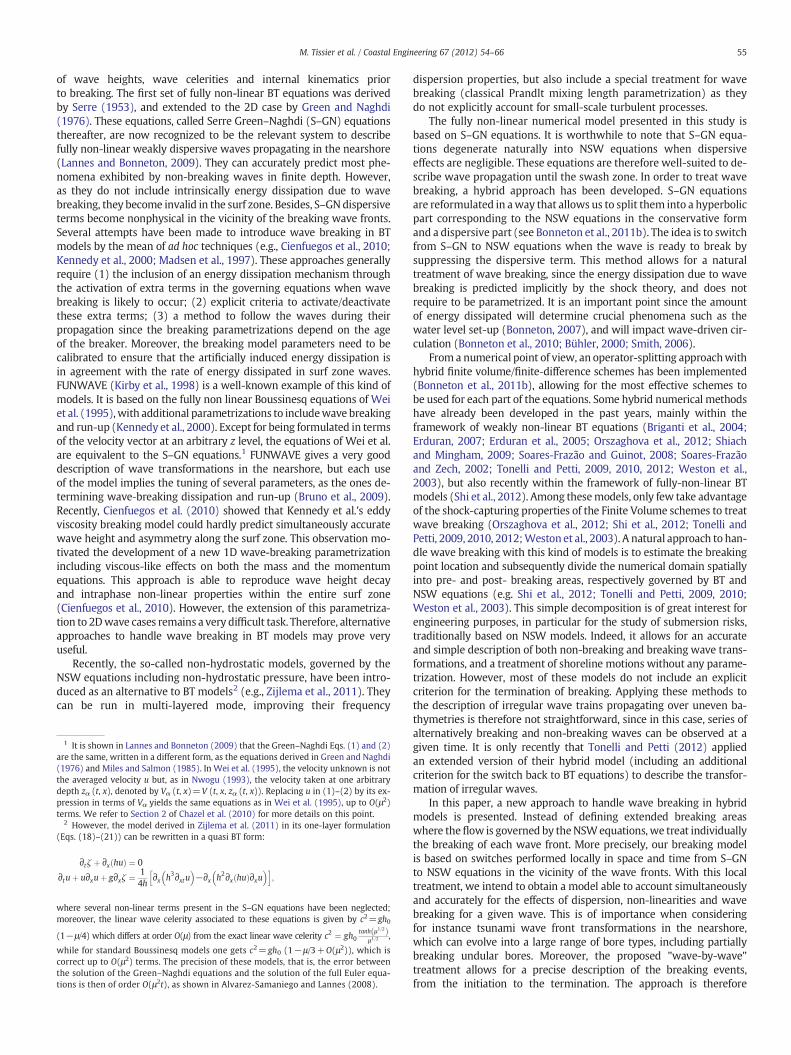
Fig. 2. Wave breaking model.

58 M. Tissier et al. / Coastal Engineering 67 (2012) 54–66

established breakers in agreement with previous experiments byDuncan (1981). Numerical tests showed that a≈2.5 was an appro-priate value. Of note, the length lNSW does not determine the amountof energy dissipated at the breaking wave front nor its spatial distri-bution. For this reason, model predictions appear to be weakly de-pendant from its value, as long as lNSW> lr.

The methodology to handle wave breaking is summarized inFig. 2. At each time step, the wave fronts are first located and theirnormalized dissipation computed following the method detailed inSection 3.1. Four cases are then possible:

• If Γb0.5 and ΦbΦi: the wave is not breaking. The flow is governedby the S–GN equations (see Fig. 2, case 1).

• If Γb0.5 and Φ≥Φi: the wave is in the first stages of breaking. Thefront is governed by NSW equations allowing the shocks to develop(case 2).

• If Γ≥0.5 and Fr1≥Frc: the wave is broken. The wave front is locallygoverned by the NSW equations (case 3).

• If Γ≥0.5 and Fr1bFrc: the wave stops breaking. The wave front isgoverned by the S–GN equations (case 4).

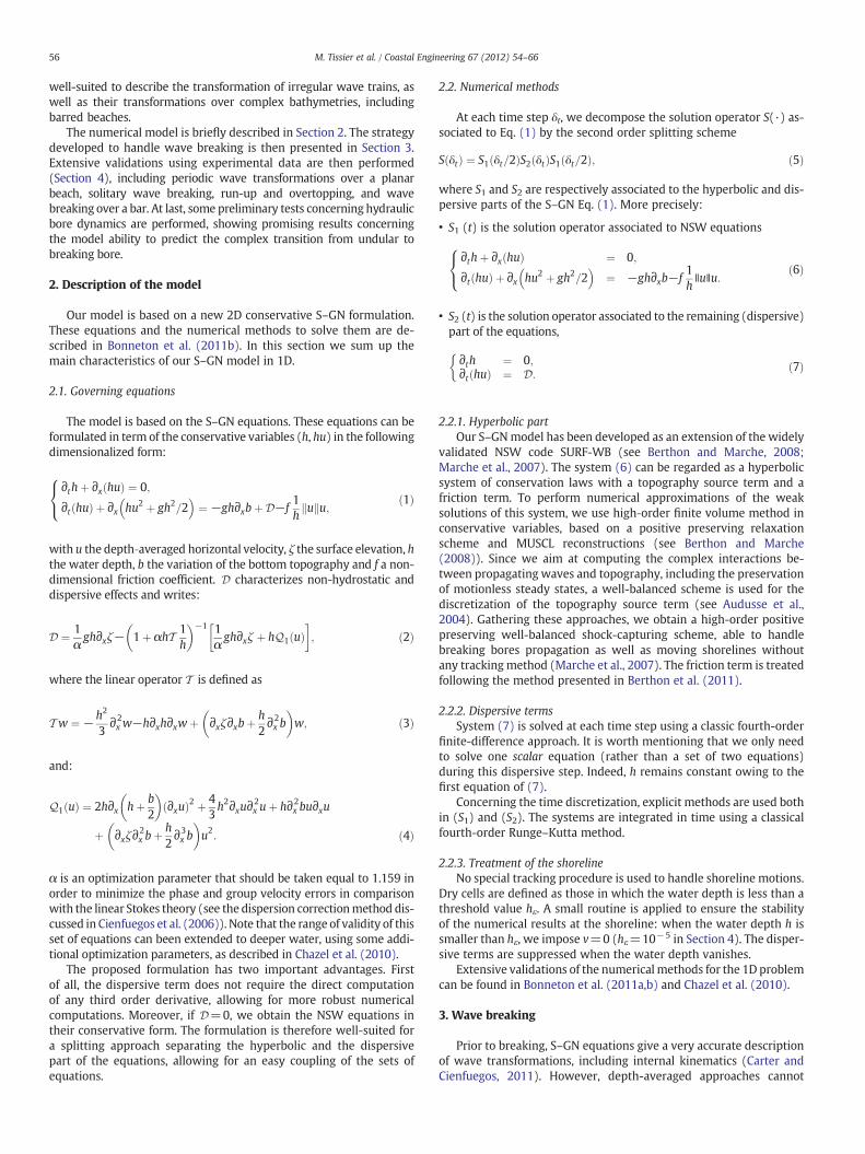
Fig. 3 illustrates our wave-by-wave treatment of breaking using asimulation corresponding to Cox (1995) regular wave experiments.In the shoaling zone, the wave fronts are characterized by a normal-ized dissipation Γ close to zero. As they propagate shoreward, thewaves gradually steepen. When their front slope reaches the criticalvalue Φi, the switch to NSW equations is performed. The wavesenter a transitional zone, where the fronts are steepening furtherwhile shocks are developing (case 2). After a while, the waves arefully broken, and their normalized dissipation is close to one (case3). They dissipate their energy while propagating shoreward, leadingto a progressive decrease of the breaker heights and front slopes. Thewaves will keep breaking as long as their Froude number is such as

0 5 100

0.2

0.4

0.6

0.8

x

h (m

)

L1

Fig. 3. Spatial snapshot of cnoidal waves propagating over a 1:35 sloping beach (Cox, 1995).governed by NSW equations.

Fr1≥Frc, i.e. until the shoreline in this case (see vertical lines inFig. 3). If the broken waves were propagating over a trough (see§4.4 for instance), the bore Froude number would decrease and even-tually get smaller than Frc. The switch back to S–GN equations wouldthen be performed (case 4), resulting in the gradual disappearance ofthe shocks and the decrease of the normalized dissipation Γ.

The transition between the two systems is performed abruptly, with-out any smooth transition zone. In this way, wave propagation is gov-erned by one given set of equations in each cell, and not by anonphysical mix of both sets. The transition generates some distur-bances, but they remain of small amplitude and do not lead to instabil-ities. No numerical filtering is applied. It is worth noting that thegeneration of oscillations is also observed for Boussinesq models basedon the surface roller method when the extra terms responsible forwave breaking are activated.

The proposed breaking model has several advantages. First, theenergy dissipation due to wave breaking is implicitly predicted bythe shock theory and does not require to be parametrized contraryto most of the BT models. Moreover, the characterization of thewaves at each time step is performed in a simple way through thestudy of the energy dissipation. The only important parameters to pre-scribe are the criteria for the initiation and termination of breaking. It isworth noting that the test cases presented in Section 4were all simulatedwith the same set of parameters (Φi=30°, Frc=1.3). The optimizationparameter α for the dispersive properties is taken equal to 1.159.

4. Validations

In order to validate ourmodel, classical test cases are first used. Theyinvolve the transformations of regular wave trains (Section 4.1) andsolitary waves (Section 4.2) over sloping beaches. These commonly-used benchmarks allow for a rigorous testing of our breaking model.More challenging test cases are then considered. The ability of ourmodel to describe wave breaking and swash motions over complexbathymetries, involving the water mass separation into disjoint waterbodies is first studied (Section 4.3). We then investigate themodel abil-ity to predict wave transformations over a bar (Section 4.4). In this testcase, a special focus is placed on the prediction of the terminationof breaking and subsequent wave transformations after the bar. Boredynamics for different Froude numbers is then studied (Section 4.5).These preliminary tests aim at investigating themodel ability to accountsimultaneously for the effects of dispersion, non-linearities and wavebreaking for a given wave.

4.1. Shoaling and breaking of regular waves over a sloping beach

4.1.1. Cox (1995)'s experimentIn our first test case we consider Cox (1995)'s regular waves ex-

periment. Cnoidal waves of relative amplitude H/h0=0.29 and period

15 20

(m)

L2 L3 L4 L5 L6

L1 to L6: locations of the wave gauges. Between 2 consecutive vertical lines, the flow is

8 10 12 14 16 18

−0.05

0

0.05

0.1

0.15

leve

ls (

m)

a

8 10 12 14 16 180

1

2

Sk

b

8 10 12 14 16 18

0

1

2

x (m)

As

c

Fig. 5. Spatial evolution of computed (lines) and experimental data (symbols) for Cox(1995) experiments. (a) ○: Mean Water Level; ▿: trough elevation relative to MWL;▵: crest elevation relative to MWL; (b) Wave skewness Sk; (c) Wave asymmetry As.The computations have been performed for different grid sizes: δx=0.04 m (solidlines), δx=0.02 m (dashed lines) and δx=0.06 m (dash-dot lines).

59M. Tissier et al. / Coastal Engineering 67 (2012) 54–66

T=2.2 s were generated in the horizontal part of a wave flume ofdepth h0=0.4 m. They were then propagating and breaking over a1:35 sloping beach. For this test case, synchronized time series offree‐surface elevation are available at six locations, corresponding towave gages located outside (L1 and L2) and inside (L3 to L6) thesurf zone (see Fig. 3). During the experiment, waves were breakingslightly shoreward to L2.

For this simulation, we choose δx=0.04 m, δt=0.01 s. Fig. 3 showsa spatial snapshot of the free-surface profile computed with themodel. It shows that the model is able to reproduce the typical saw-tooth profile in the Inner Surf Zone (ISZ). Fig. 4 compares the experi-mental and numerical time series of free-surface elevation for thisexperiment. We can see that we have a good overall agreement inboth the shoaling and surf zones. Themain discrepancies are observedin the vicinity of the breaking point, where themaximumwave heightis underestimated. We can also notice that the numerical brokenwave fronts are a bit too steep: this aspect will be discussed laterin this section. It is worth noting that the time series are in phasefor most of the wave gauges, demonstrating that wave celerity iswell predicted by the model. The short time lag observed at the mostonshore location (L6) is a consequence of the slight underestimationof the computed wave height in the inner surf zone (see also Fig. 5a,plain lines).

In particular, the model ability to describe non-linear wave shapeis assessed through the computation of the crest-trough asymmetryor wave skewness parameter, Sk, and the left-right asymmetry pa-rameter, As, defined as (Kennedy et al., 2000):

Sk ¼ζ−�ζ �3D Eζ−�ζ �2D E3=2 ð11Þ

As ¼ −H ζ−�ζ �3D E

ζ−�ζ �2D E3=2 ; ð12Þ

where �ζ is the wave-averaged surface elevation, ⟨⟩ the time-averagingoperator and H the Hilbert transform.

3 4 5 6−0.05

0

0.05

0.1

L1

ζ (m

)

3 4 5 6−0.05

0

0.05

0.1

L2

3 4 5 6−0.05

0

0.05

0.1

L3

ζ (m

)

3 4 5 6−0.05

0

0.05

0.1

L4

3 4 5 6−0.05

0

0.05

0.1

L5

t (s)

ζ (m

)

3 4 5 6−0.05

0

0.05

0.1

L6

t (s)

Fig. 4. Comparisons of computed (solid lines) and experimental (dashed lines) syn-chronized time series of free-surface elevation at the wave gauges for Cox (1995)breaking experiment (δx=0.04 m and δt=0.01 s).

It is well-known that once the waves are broken and representedas shocks, the front steepness depends on the spatial resolution δx. Inorder to evaluate how the grid spacing affects the model predictions,the numerical results obtained for two additional grid sizes arealso displayed in Fig. 5 (δx=0.02 m and 0.06 m, with δt=0.01 sfor all the computations). Fig. 5a shows that all the simulations un-derestimate the wave height at breaking, but predict similar locationsof the breaking point, in agreement with the experimental data. It canbe observed that the maximal wave crest elevation before breakingincreases while the grid size decreases, leading to differences in thewave height predictions in the first stages of breaking. These differ-ences result from the larger numerical dissipation for the simulationsperformed with the coarser grids, and are therefore not due to theshock-capturing properties of our model (see also Shi et al. (2012)for similar conclusions using their fully non-linear BT hybrid model).We can moreover see that the agreement between data and modelis good concerning the prediction of wave set-up. As wave set-upand broken wave energy dissipation are closely related (Bonneton,2007), this result demonstrates that the model gives a realistic de-scription of the energy dissipation.

Concerning the wave shape, Fig. 5b,c shows that the wave skew-ness and asymmetry are well described before breaking for the 3grid sizes, but that the discrepancies increase in the surf zone. Thewave skewness is still relatively well predicted after breaking, evenif a slight underestimation of this parameter is generally observed.Larger discrepancies between experimental and numerical data canbe observed for the asymmetry in the surf zone. The model predictsa too large increase of As in the first stages of breaking. It correspondsto the steepening of the fronts following the switch from S–GN toNSW equations, and therefore to the shock development. Once the

4 6 8 10 12 14 16

−0.05

0

0.05

0.1

0.15

leve

ls (

m)

a

4 6 8 10 12 14 160

1

2

Sk

b

4 6 8 10 12 14 16

0

1

2

As

x (m)

c

Fig. 7. Spatial evolution of computed (lines) and experimental data (symbols) for Tingand Kirby (1994) spilling breaking experiment. (a) ○: spatial evolution of the meanwater level; ▿: trough elevation relative to MWL; ▵: crest elevation relative to MWL.(b) Wave skewness. (c) Wave asymmetry.

60 M. Tissier et al. / Coastal Engineering 67 (2012) 54–66

breaker is fully-developed, the predicted asymmetry stays almostconstant, while the asymmetry computed from the experimentaldata keeps increasing progressively. As expected, the value of Asincreases for decreasing spatial resolution. It is important to keep inmind that the inaccuracies observed in term of asymmetry of thebreaking wave front are not specific to our model, but result fromthe description of breaking wave fronts as shocks by the NSW equa-tions. The choice of δx is therefore crucial to obtain a good order ofmagnitude for the wave asymmetry in the surf zone. As the gridsize determines the length of the numerical roller (represented as ashock), the model abilities could probably be improved by relatingδx to the physical length of the roller, which can be seen as roughlyproportional to the characteristic water depth. The use of a variablegrid size with δx proportional to the characteristic depth could thenlead to a better prediction of the left-right asymmetry by the model.

4.1.2. Ting and Kirby (1994)'s experimentIn this section the numerical model is applied to reproduce

the laboratory experiments performed by Ting and Kirby (1994) forspilling breakers. Cnoidal waves were generated in the horizontalpart of a flume (h0=0.4 m) and were propagating over a 1:35 slopingbeach. The wave period was T=2.0 s and the incident wave heightH=0.125 m. For this experiment, non-synchronized time series ofsurface elevations and mean characteristic levels (crest, trough andmean water levels) are available at 21 locations in the shoaling andsurf zones. For the simulation, the grid size of the mesh is δx=0.05 mand the time step is δt=0.01 s.

Fig. 6 compares the time series of free‐surface elevations at differentlocations, in the shoaling and breaking zone. The main discrepanciesare found in the vicinity of the breaking point, where the wave heightis underestimated, but the overall agreement improves significantlywhile propagating shoreward.

Fig. 7a shows the spatial variations of the crest and trough eleva-tions, as well as the variation of the mean water level for the

0 2 4−0.05

0

0.05

0.1

0 2 4−0.05

0

0.05

0.1

0 2 4−0.05

0

0.05

0.1

0 2 4−0.05

0

0.05

0.1

0 2 4−0.05

0

0.05

0.1

0 2 4−0.05

0

0.05

0.1

0 2 4−0.05

0

0.05

0.1

0 2 4−0.05

t (s)

x =12.5 m x =14.5 m x =16.5 m

x =10 m x =11 m x =12 m

x =4 m x =6 m x =6 m

t (s) t (s)

0

0.05

0.1

0 2 4−0.05

0

0.05

0.1

(m)

(m)

(m)

Fig. 6. Comparisons of computed (solid lines) and measured (dashed lines) time series of free‐surface elevations for Ting and Kirby experiment at different locations.

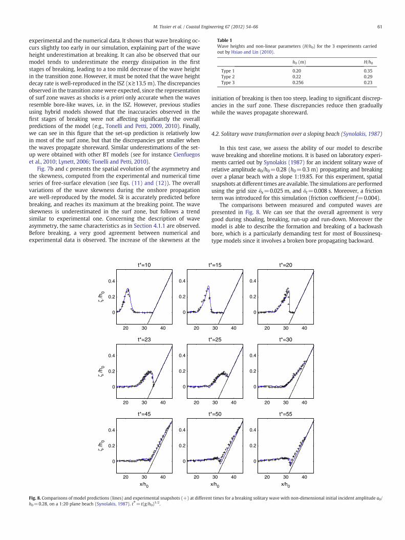
Table 1Wave heights and non-linear parameters (H/h0) for the 3 experiments carriedout by Hsiao and Lin (2010).

h0 (m) H/h0

Type 1 0.20 0.35Type 2 0.22 0.29Type 3 0.256 0.23

61M. Tissier et al. / Coastal Engineering 67 (2012) 54–66

experimental and the numerical data. It shows that wave breaking oc-curs slightly too early in our simulation, explaining part of the waveheight underestimation at breaking. It can also be observed that ourmodel tends to underestimate the energy dissipation in the firststages of breaking, leading to a too mild decrease of the wave heightin the transition zone. However, it must be noted that the wave heightdecay rate is well-reproduced in the ISZ (x≳13.5 m). The discrepanciesobserved in the transition zonewere expected, since the representationof surf zone waves as shocks is a priori only accurate when the wavesresemble bore-like waves, i.e. in the ISZ. However, previous studiesusing hybrid models showed that the inaccuracies observed in thefirst stages of breaking were not affecting significantly the overallpredictions of the model (e.g., Tonelli and Petti, 2009, 2010). Finally,we can see in this figure that the set-up prediction is relatively lowin most of the surf zone, but that the discrepancies get smaller whenthe waves propagate shoreward. Similar underestimations of the set-up were obtained with other BT models (see for instance Cienfuegoset al., 2010; Lynett, 2006; Tonelli and Petti, 2010).

Fig. 7b and c presents the spatial evolution of the asymmetry andthe skewness, computed from the experimental and numerical timeseries of free‐surface elevation (see Eqs. (11) and (12)). The overallvariations of the wave skewness during the onshore propagationare well‐reproduced by the model. Sk is accurately predicted beforebreaking, and reaches its maximum at the breaking point. The waveskewness is underestimated in the surf zone, but follows a trendsimilar to experimental one. Concerning the description of waveasymmetry, the same characteristics as in Section 4.1.1 are observed.Before breaking, a very good agreement between numerical andexperimental data is observed. The increase of the skewness at the

20 30 40

0

0.2

0.4

t*=10

ζ /h

0ζ

/h0

ζ /h

0

20

0

0.2

0.4

t

20 30 40

0

0.2

0.4

t*=23

20

0

0.2

0.4

t

20 30 40

0

0.2

0.4

t*=45

x/h0

20

0

0.2

0.4

t

Fig. 8. Comparisons of model predictions (lines) and experimental snapshots (+) at differenh0=0.28, on a 1:20 plane beach (Synolakis, 1987). t⁎= t(g/h0)1/2.

initiation of breaking is then too steep, leading to significant discrep-ancies in the surf zone. These discrepancies reduce then graduallywhile the waves propagate shoreward.

4.2. Solitary wave transformation over a sloping beach (Synolakis, 1987)

In this test case, we assess the ability of our model to describewave breaking and shoreline motions. It is based on laboratory experi-ments carried out by Synolakis (1987) for an incident solitary wave ofrelative amplitude a0/h0=0.28 (h0=0.3 m) propagating and breakingover a planar beach with a slope 1:19.85. For this experiment, spatialsnapshots at different times are available. The simulations are performedusing the grid size δx=0.025 m, and δt=0.008 s. Moreover, a frictionterm was introduced for this simulation (friction coefficient f=0.004).

The comparisons between measured and computed waves arepresented in Fig. 8. We can see that the overall agreement is verygood during shoaling, breaking, run-up and run-down. Moreover themodel is able to describe the formation and breaking of a backwashbore, which is a particularly demanding test for most of Boussinesq-type models since it involves a broken bore propagating backward.

30 40

*=15

20 30 40

0

0.2

0.4

t*=20

30 40

*=25

20 30 40

0

0.2

0.4

t*=30

30 40

*=50

x/h0

20 30 40

0

0.2

0.4

t*=55

x/h0

t times for a breaking solitary wave with non-dimensional initial incident amplitude a0/

50

0.2

0.41 3 10 15 22 28 37-40 46

6 7 8x (m)

z (m

)

9 10 11 12

Fig. 9. Schematic view of the experimental set‐up in Hsiao and Lin (2010). Vertical lines: location of the wave gauges (WG). Horizontal lines: water levels at rest for the three typesof solitary waves described in Table 1.

62 M. Tissier et al. / Coastal Engineering 67 (2012) 54–66

4.3. Solitary waves overtopping a seawall (Hsiao and Lin, 2010)

We investigate here the ability of our model to describe the com-plex transformations of solitary waves overtopping a seawall. Weconsider experiments carried out by Hsiao and Lin (2010) in a 22 mlong wave flume located in the Tainan Hydraulic Laboratory, NationalCheug Kung University, Taiwan. During this experiment, three typesof solitary waves were generated. Their characteristics are describedin Table 1 (see Fig. 9 for the visualization of the water depth at restfor the 3 cases). In the first case, the solitary wave was breakingon the sloping beach before reaching the wall. In the second case,the solitary wave was breaking on the seawall whereas for case 3the wave was overtopping directly the seawall without any priorbreaking and subsequently collapsing behind the seawall. Hsiao andLin compared the experimental data with predictions with the

2 4 62 4 6 8

t (s)10 12

2 4 62 4 6 8 10 12

2 4 62 4 6 8 10 12

2 4 62 4 6 8 10 12

2 4 62 4 6 8 10 12

0 2 4 6 8 10 0 2 4

-2 -1-2

0.1Type 1: h0=0.20 m Type 2: h

0.05

0

0.1

0.05

0

0.1

0.05

0

0.1

0.05

0

0.1

0.05

0

0.1

0.05

0

0.1

0.05

0

0.1

0.05

0

0.1

0.05

0

0.1

0.05

0

0.1

0.05

0

0.1

0.05

0

0.1

0.05

0

0.1

0.05

0

-1 0 1 2

WGI

WG3

WG10

WG22

WG28

WG37

WG40

ζ (m

)ζ

(m)

ζ (m

)ζ

(m)

ζ (m

)ζ

(m)

ζ (m

)

Fig. 10. Comparison between experimental (○) and numerical (plain lines) time series of fLin, 2010).

volume of fluid (VOF) type model COBRAS (Lin and Liu, 1998), basedon Reynolds-Averaged Navier–Stokes equations with k−ε turbulentclosure. They found a very good agreement between experimentaldata and model predictions, for all stages of wave transformations.This test case will allow us to evaluate the degree of accuracy reachableusing a depth-averaged model only.

For our simulations, we choose δt=0.007 s and δx=0.02 m. Aquadratic friction term is introduced, with a coefficient f=0.01. Aswe assume the dispersive effects not to be significant shoreward ofthe seawall, we decided to suppress them in this entire region. Thisalso prevents the potential development of numerical instabilities atthe multiple boundaries between land and water in this case.

Comparisons between the measured and numerical time series offree-surface elevations at the wave gauges are presented in Fig. 10 forthe three types of solitary waves. A very good agreement is obtained

2 4 6 8

t (s)10 128

t (s)10 12

2 4 6 8 10 128 10 12

2 4 6 8 10 128 10 12

2 4 6 8 10 128 10 12

2 4 6 8 10 128 10 12

6 8 10 0 2 4 6 8 10

-2 -1 0 1 20 1 2

0=0.22 m Type 3: h0=0.256 m0.1

0.05

0

0.1

0.05

0

0.1

0.05

0

0.1

0.05

0

0.1

0.05

0

0.1

0.05

0

0.1

0.05

0

WGI WGI

WG3 WG3

WG15 WG22

WG22 WG38

WG28 WG39

WG37 WG40

WG39 WG46

ree-surface elevation for the 3 types of solitary waves described in Table 1 (Hsiao and

0 2 4 6 8 10−0.05

0

0.05

ζ (m

)

WG 1

0 2 4 6 8 10−0.05

0

0.05

ζ (m

)

WG 2

0 2 4 6 8 10−0.05

0

0.05

ζ (m

)

WG 3

0 2 4 6 8 10−0.05

0

0.05

ζ (m

)

WG 4

0 2 4 6 8 10−0.05

0

0.05

ζ (m

)

WG 5

0 2 4 6 8 10−0.05

0

0.05ζ

(m)

WG 6

0 2 4 6 8 10−0.05

0

0.05

ζ (m

)

WG 7

0 2 4 6 8 10−0.05

0

0.05

ζ (m

)

WG 8

t (s)

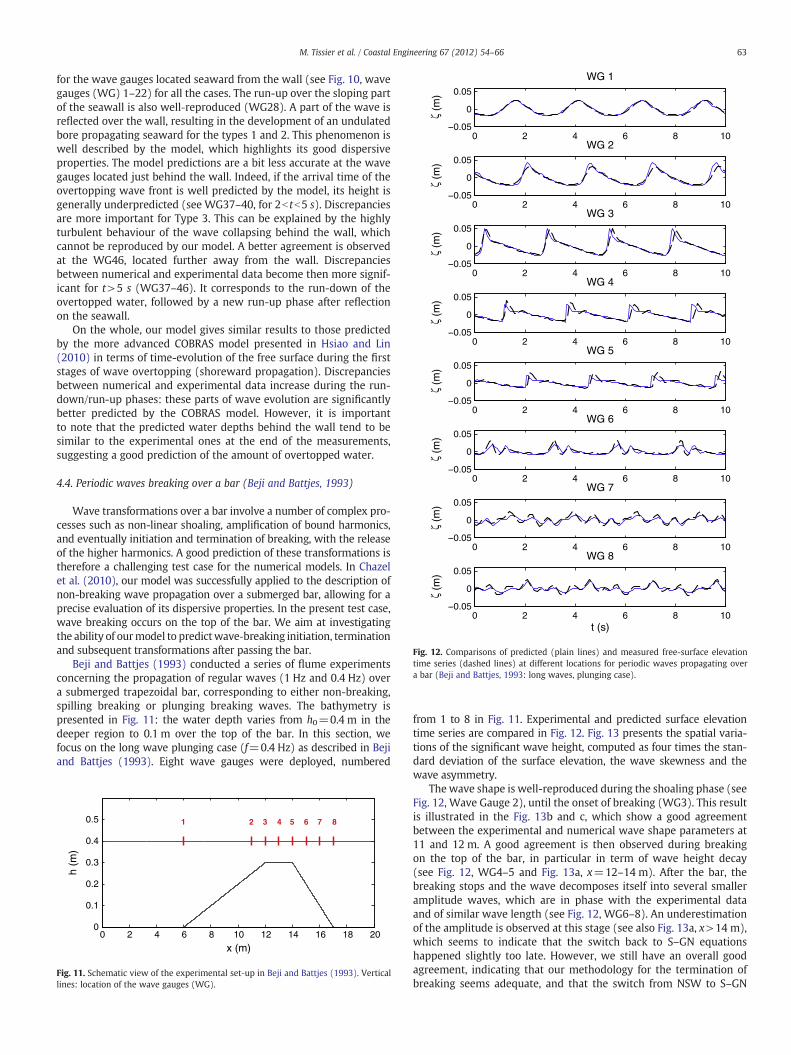
Fig. 12. Comparisons of predicted (plain lines) and measured free-surface elevationtime series (dashed lines) at different locations for periodic waves propagating overa bar (Beji and Battjes, 1993: long waves, plunging case).

63M. Tissier et al. / Coastal Engineering 67 (2012) 54–66

for the wave gauges located seaward from the wall (see Fig. 10, wavegauges (WG) 1–22) for all the cases. The run-up over the sloping partof the seawall is also well‐reproduced (WG28). A part of the wave isreflected over the wall, resulting in the development of an undulatedbore propagating seaward for the types 1 and 2. This phenomenon iswell described by the model, which highlights its good dispersiveproperties. The model predictions are a bit less accurate at the wavegauges located just behind the wall. Indeed, if the arrival time of theovertopping wave front is well predicted by the model, its height isgenerally underpredicted (see WG37–40, for 2b tb5 s). Discrepanciesare more important for Type 3. This can be explained by the highlyturbulent behaviour of the wave collapsing behind the wall, whichcannot be reproduced by our model. A better agreement is observedat the WG46, located further away from the wall. Discrepanciesbetween numerical and experimental data become then more signif-icant for t>5 s (WG37–46). It corresponds to the run-down of theovertopped water, followed by a new run-up phase after reflectionon the seawall.

On the whole, our model gives similar results to those predictedby the more advanced COBRAS model presented in Hsiao and Lin(2010) in terms of time-evolution of the free surface during the firststages of wave overtopping (shoreward propagation). Discrepanciesbetween numerical and experimental data increase during the run-down/run-up phases: these parts of wave evolution are significantlybetter predicted by the COBRAS model. However, it is importantto note that the predicted water depths behind the wall tend to besimilar to the experimental ones at the end of the measurements,suggesting a good prediction of the amount of overtopped water.

4.4. Periodic waves breaking over a bar (Beji and Battjes, 1993)

Wave transformations over a bar involve a number of complex pro-cesses such as non-linear shoaling, amplification of bound harmonics,and eventually initiation and termination of breaking, with the releaseof the higher harmonics. A good prediction of these transformations istherefore a challenging test case for the numerical models. In Chazelet al. (2010), our model was successfully applied to the description ofnon-breaking wave propagation over a submerged bar, allowing for aprecise evaluation of its dispersive properties. In the present test case,wave breaking occurs on the top of the bar. We aim at investigatingthe ability of ourmodel to predictwave‐breaking initiation, terminationand subsequent transformations after passing the bar.

Beji and Battjes (1993) conducted a series of flume experimentsconcerning the propagation of regular waves (1 Hz and 0.4 Hz) overa submerged trapezoidal bar, corresponding to either non-breaking,spilling breaking or plunging breaking waves. The bathymetry ispresented in Fig. 11: the water depth varies from h0=0.4 m in thedeeper region to 0.1 m over the top of the bar. In this section, wefocus on the long wave plunging case (f=0.4 Hz) as described in Bejiand Battjes (1993). Eight wave gauges were deployed, numbered

0 2 4 6 8 10 12 14 16 18 200

0.1

0.2

0.3

0.4

0.5

x (m)

h (m

)

1 2 3 4 5 6 7 8

Fig. 11. Schematic view of the experimental set‐up in Beji and Battjes (1993). Verticallines: location of the wave gauges (WG).

from 1 to 8 in Fig. 11. Experimental and predicted surface elevationtime series are compared in Fig. 12. Fig. 13 presents the spatial varia-tions of the significant wave height, computed as four times the stan-dard deviation of the surface elevation, the wave skewness and thewave asymmetry.

The wave shape is well-reproduced during the shoaling phase (seeFig. 12, Wave Gauge 2), until the onset of breaking (WG3). This resultis illustrated in the Fig. 13b and c, which show a good agreementbetween the experimental and numerical wave shape parameters at11 and 12 m. A good agreement is then observed during breakingon the top of the bar, in particular in term of wave height decay(see Fig. 12, WG4–5 and Fig. 13a, x=12–14 m). After the bar, thebreaking stops and the wave decomposes itself into several smalleramplitude waves, which are in phase with the experimental dataand of similar wave length (see Fig. 12, WG6–8). An underestimationof the amplitude is observed at this stage (see also Fig. 13a, x>14 m),which seems to indicate that the switch back to S–GN equationshappened slightly too late. However, we still have an overall goodagreement, indicating that our methodology for the termination ofbreaking seems adequate, and that the switch from NSW to S–GN

60 80 100 120 140 160 180−1

0

1

2

ζ/(h

2−h 1)

ζ/(h

2−h 1)

ζ/(h

2−h 1)

ζ/(h

2−h 1)

ζ/(h

2−h 1)

Fr = 1.10

60 80 100 120 140 160 180−1

0

1

2

Fr = 1.35

60 80 100 120 140 160 180−1

0

1

2

Fr = 1.40

60 80 100 120 140 160 180−1

0

1

2

Fr = 1.45

60 80 100 120 140 160 180−1

0

1

2

x (m)

Fr = 1.90

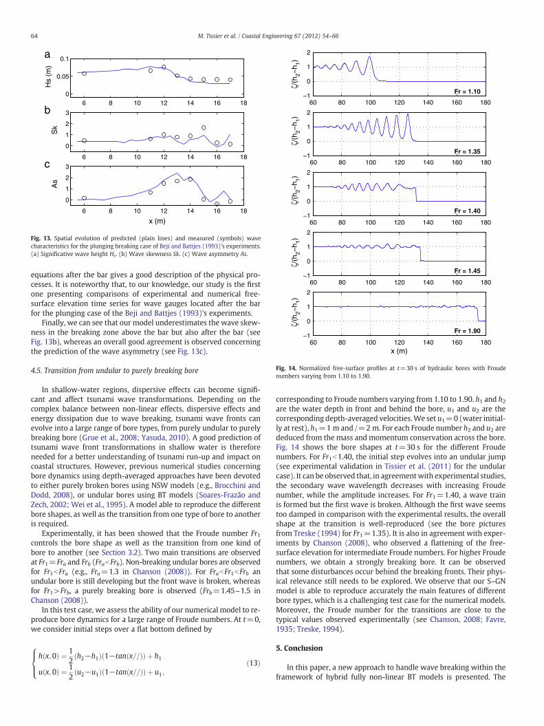
Fig. 14. Normalized free‐surface profiles at t=30 s of hydraulic bores with Froudenumbers varying from 1.10 to 1.90.

6 8 10 12 14 16 180

0.05

0.1

Hs

(m)

a

6 8 10 12 14 16 18

0

1

2

3

As

x (m)

c6 8 10 12 14 16 18

0

1

2

3

Sk

b

Fig. 13. Spatial evolution of predicted (plain lines) and measured (symbols) wavecharacteristics for the plunging breaking case of Beji and Battjes (1993)'s experiments.(a) Significative wave height Hs. (b) Wave skewness Sk. (c) Wave asymmetry As.

64 M. Tissier et al. / Coastal Engineering 67 (2012) 54–66

equations after the bar gives a good description of the physical pro-cesses. It is noteworthy that, to our knowledge, our study is the firstone presenting comparisons of experimental and numerical free‐surface elevation time series for wave gauges located after the barfor the plunging case of the Beji and Battjes (1993)'s experiments.

Finally, we can see that our model underestimates the wave skew-ness in the breaking zone above the bar but also after the bar (seeFig. 13b), whereas an overall good agreement is observed concerningthe prediction of the wave asymmetry (see Fig. 13c).

4.5. Transition from undular to purely breaking bore

In shallow-water regions, dispersive effects can become signifi-cant and affect tsunami wave transformations. Depending on thecomplex balance between non-linear effects, dispersive effects andenergy dissipation due to wave breaking, tsunami wave fronts canevolve into a large range of bore types, from purely undular to purelybreaking bore (Grue et al., 2008; Yasuda, 2010). A good prediction oftsunami wave front transformations in shallow water is thereforeneeded for a better understanding of tsunami run-up and impact oncoastal structures. However, previous numerical studies concerningbore dynamics using depth-averaged approaches have been devotedto either purely broken bores using NSW models (e.g., Brocchini andDodd, 2008), or undular bores using BT models (Soares-Frazão andZech, 2002; Wei et al., 1995). A model able to reproduce the differentbore shapes, as well as the transition from one type of bore to anotheris required.

Experimentally, it has been showed that the Froude number Fr1controls the bore shape as well as the transition from one kind ofbore to another (see Section 3.2). Two main transitions are observedat Fr1=Fra and Frb (FrabFrb). Non-breaking undular bores are observedfor Fr1bFra (e.g., Fra=1.3 in Chanson (2008)). For FrabFr1bFrb anundular bore is still developing but the front wave is broken, whereasfor Fr1>Frb, a purely breaking bore is observed (Frb=1.45–1.5 inChanson (2008)).

In this test case, we assess the ability of our numerical model to re-produce bore dynamics for a large range of Froude numbers. At t=0,we consider initial steps over a flat bottom defined by

h x;0ð Þ ¼ 12

h2−h1ð Þ 1−tan x==ð Þð Þ þ h1

u x;0ð Þ ¼ 12

u2−u1ð Þ 1−tan x==ð Þð Þ þ u1;

8><>: ð13Þ

corresponding to Froude numbers varying from 1.10 to 1.90. h1 and h2are the water depth in front and behind the bore, u1 and u2 are thecorresponding depth-averaged velocities.We set u1=0 (water initial-ly at rest), h1=1 m and /=2m. For each Froude number h2 and u2 arededuced from the mass and momentum conservation across the bore.Fig. 14 shows the bore shapes at t=30 s for the different Froudenumbers. For Fr1b1.40, the initial step evolves into an undular jump(see experimental validation in Tissier et al. (2011) for the undularcase). It can be observed that, in agreementwith experimental studies,the secondary wave wavelength decreases with increasing Froudenumber, while the amplitude increases. For Fr1=1.40, a wave trainis formed but the first wave is broken. Although the first wave seemstoo damped in comparison with the experimental results, the overallshape at the transition is well-reproduced (see the bore picturesfrom Treske (1994) for Fr1=1.35). It is also in agreement with exper-iments by Chanson (2008), who observed a flattening of the free-surface elevation for intermediate Froude numbers. For higher Froudenumbers, we obtain a strongly breaking bore. It can be observedthat some disturbances occur behind the breaking fronts. Their phys-ical relevance still needs to be explored. We observe that our S–GNmodel is able to reproduce accurately the main features of differentbore types, which is a challenging test case for the numerical models.Moreover, the Froude number for the transitions are close to thetypical values observed experimentally (see Chanson, 2008; Favre,1935; Treske, 1994).

5. Conclusion

In this paper, a new approach to handle wave breaking within theframework of hybrid fully non-linear BT models is presented. The

65M. Tissier et al. / Coastal Engineering 67 (2012) 54–66

model has been developed as an extension of the well-validated NSWshock-capturing code SURF-WB (Marche et al., 2007), using hybridfinite volume/finite‐difference schemes (Bonneton et al., 2011b).

The modeling strategy for wave breaking is based on the splittingof S–GN equations between a hyperbolic part corresponding to theNSWE and a dispersive term. When the wave is ready to break, weswitch locally to the NSWE by skipping the dispersive step, such asbroken wave fronts can be described as shocks. Energy dissipationdue to wave breaking is then predicted by the shock theory, and donot require to be parametrized. The characterization of wave frontsat each time step is easily performed through the study of local ener-gy dissipation. Combined with simple criteria for the initiation andtermination of breaking, we obtain an efficient treatment of wavebreaking and broken waves propagation without any complex algo-rithm to follow the waves. Ourmethod has been extensively validatedwith laboratory data. The ability of our model to reproduce regularwave transformation over slopping beaches has been thoroughly in-vestigated. Application of the model to several cases of overtoppingover a seawall and to a case of wave propagation over a bar allowedus to evaluate the model ability to describe wave transformation overcomplex bathymetries. Finally, promising tests concerning hydraulicbore dynamics were performed, showing that the model is able toreproduce the transitions from undular to purely breaking bores. Thestudy of bore dynamics is a particularly challenging test case since itresults from the complex balance between non-linearities, dispersiveeffects and energy dissipation due to wave breaking.

Work is in progress concerning the 2DH extension of the model.The splitting method used in this model, initially presented inBonneton et al. (2011b), can be easily extended to 2DH. Its imple-mentation is in progress. The new 2DH S–GN code could be a power-ful tool to study the generation of wave-induced circulations andmacro-vortices, which are mainly controlled by alongshore variationsin breaking wave energy dissipation (Bonneton et al., 2010; Peregrine,1998).

Acknowledgments

The authors would like to thank Prof. Shih-Chun Hsiao and Ting-Chieh Lin, as well as Prof. Serdar Beji and Prof. Jurjen A. Battjes forproviding the experimental data. The authors would like to acknowl-edge the ANR-funded project MISEEVA, which funded M. Tissier'sPhD thesis, and the scientific support of Dr. Rodrigo Pedreros. Theauthors would also like to acknowledge additional financial andscientific support of the French INSU—CNRS (Institut National desSciences de l'Univers—Centre National de la Recherche Scientifique)program IDAO ("Interactions et Dynamique de l'Atmosphère et del'Océan"), as well as the ANR-funded project MathOcean (ANR-09-BLAN-0301-01).

References

Alvarez-Samaniego, B., Lannes, D., 2008. Large time existence for 3D water-waves andasymptotics. Invent. Math. 171, 485–541.

Audusse, E., Bouchut, F., Bristeau, M., Klein, R., Perthame, B., 2004. A fast and stablewell-balanced scheme with hydrostatic reconstruction for shallow water flows.SIAM Journal on Scientific Computing 25, 2050–2065.

Beji, S., Battjes, J.A., 1993. Experimental investigation of wave propagation over a bar.Coastal Engineering 19, 151–162.

Berthon, C., Marche, F., 2008. A positive preserving high order VFRoe scheme forshallow water equations: a class of relaxation schemes. SIAM Journal on ScientificComputing 30, 2587–2612.

Berthon, C., Marche, F., Turpault, R., 2011. An efficient scheme on wet/dry transitionsfor shallow water equations with friction. Computer and Fluids 48.

Bjørkavåg, M., Kalisch, H., 2011. Wave breaking in Boussinesq models for undularbores. Physics Letters A 375, 1570–1578.

Bonneton, P., 2007. Modelling of periodic wave transformation in the inner surf zone.Ocean Engineering 34, 1459–1471.

Bonneton, P., Bruneau, N., Marche, F., Castelle, B., 2010. Large-scale vorticity generationdue to dissipating waves in the surf zone. Discrete and Continuous DynamicalSystems—Series B 13, 729–738.

Bonneton, P., Barthelemy, E., Chazel, F., Cienfuegos, R., Lannes, D., Marche, F., Tissier, M.,2011a. Recent advances in Serre-Green Naghdi modelling for wave transformation,breaking and runup processes. European Journal of Mechanics—B/Fluids 30, 589–597.

Bonneton, P., Chazel, F., Lannes, D., Marche, F., Tissier, M., 2011b. A splitting approachfor the fully nonlinear and weakly dispersive Green–Naghdi model. Journal ofComputational Physics 230, 1479–1498.

Briganti, R., Brocchini, M., Bernetti, R., 2004. An operator-splitting approach forBoussinesq-type equations. GIMC 2004, XV Congresso Italiano di MeccanicaComputazionale–AIMETA.

Brocchini, M., Dodd, N., 2008. Nonlinear shallow water equation modeling for coastalengineering. Journal of Waterway, Port, Coastal, and Ocean Engineering 134,104–120.

Bruno, D., Serio, F.D., Mossa, M., 2009. The FUNWAVE model application and its valida-tion using laboratory data. Coastal Engineering 56, 773–787.

Bühler, O., 2000. On the vorticity transport due to dissipating or breaking waves inshallow-water flow. Journal of Fluid Mechanics 407, 235–263.

Carter, J.D., Cienfuegos, R., 2011. The kinematics and stability of solitary and cnoidalwave solutions of the Serre equations. European Journal of Mechanics - B/Fluids30, 259–268.

Chanson, H., 2008. Turbulence in positive surges and tidal bores. effects of bed rough-ness and adverse bed slopes. Hydraulic Model Report No. CH68/08 Div. of CivilEngineering, The University of Queensland, Brisbane, Australia. 121 pages.

Chazel, F., Lannes, D.,Marche, F., 2010. Numerical simulation of strongly nonlinear and dis-persive waves using a Green–Naghdi model. Journal of Scientific Computing 1–12.

Cienfuegos, R., Barthélemy, E., Bonneton, P., 2006. A fourth-order compact finite volumescheme for fully nonlinear and weakly dispersive Boussinesq-type equations. Part I:model development and analysis. International Journal for Numerical Methods inFluids 51, 1217–1253.

Cienfuegos, R., Barthélemy, E., Bonneton, P., 2010. Wave-breaking model for Boussinesq-type equations including roller effects in the mass conservation equation. Journal ofWaterway, Port, Coastal, and Ocean Engineering 136, 10–26.

Cox, D.T., 1995. Experimental and numerical modelling of surf zone hydrodynamics.Ph.D. thesis. University of Delaware, Newark, Del.

Duncan, J.H., 1981. An experimental investigation of breaking waves produced by atowed hydrofoil. Proceedings of the Royal Society of London. Series A 377, 331–348.

Elgar, S., Gallagher, E.L., Guza, R.T., 2001. Nearshore sandbar migration. Journal ofGeophysical Research 106 (C6), 11623–11627.

Erduran, K.S., 2007. Further application of hybrid solution to another form of Boussinesqequations and comparisons. International Journal for Numerical Methods in Fluids53, 827–849.

Erduran, K.S., Ilic, S., Kutija, V., 2005. Hybrid finite-volume finite-difference scheme forthe solution of Boussinesq equations. International Journal for Numerical Methodsin Fluids 49, 1213–1232.

Favre, H., 1935. Etude théorique et expérimentale des ondes de translation dans lescanaux découverts. Dunod, Paris.

Grasso, F., Michallet, H., Barthélemy, E., 2011. Sediment transport associated with mor-phological beach changes forced by irregular asymmetric, skewed waves. Journalof Geophysical Research 116.

Green, A.E., Naghdi, P.M., 1976. A derivation of equations for wave propagation in waterof variable depth. Journal of Fluid Mechanics 78, 237–246.

Grue, J., Pelinovsky, E.N., Fructus, D., Talipova, T., Kharif, C., 2008. Formation of undularbores and solitary waves in the Strait of Malacca caused by the 26 December 2004Indian Ocean tsunami. Journal of Geophysical Research C: Oceans 113.

Haller, M.C., Catalán, P.A., 2010. Remote sensing of wave roller lengths in the laboratory.Journal of Geophysical Research 114.

Hsiao, S.C., Lin, T.C., 2010. Tsunami-like solitary waves impinging and overtopping animpermeable seawall: experiment and RANS modeling. Coastal Engineering 57,1–18.

Kennedy, A.B., Chen, Q., Kirby, J.T., Dalrymple, R.A., 2000. Boussinesq modeling of wavetransformation, breaking and run-up. I: one dimension. ASCE Journal of Waterway,Port, Coastal and Ocean Engineering 126 (1), 48–56.

Kirby, J.T., Wei, G., Chen, Q., Kennedy, A.B., Dalrymple, R.A., 1998. FUNWAVE 1.0. Fullynonlinear Boussinesq wave model. Documentation and user's manual. TechnicalReport CACR-98-06Center for Applied Coastal Research, Department of Civil andEnvironmental Engineering, University of Delaware.

Kobayashi, N., Silva, G.D., Watson, K., 1989. Wave transformation and swash oscillationon gentle and steep slopes. Journal of Geophysical Research 94, 951–966.

Lannes, D., Bonneton, P., 2009. Derivation of asymptotic two-dimensional time-dependent equations for surface water wave propagation. Physics of Fluids 21.

Lin, P., Liu, P.L.F., 1998. A numerical study of breaking waves in the surf zone. Journal ofFluid Mechanics 359, 239–264.

Lynett, P.J., 2006. Nearshore wave modeling with high-order Boussinesq-type equa-tions. Journal of Waterway, Port, Coastal and Ocean Engineering 132.

Madsen, P.A., Sørensen, O.R., Schäffer, H.A., 1997. Surf zone dynamics simulated by aBoussinesq type model. Part I. Model description and cross-shore motion of regularwaves. Coastal Engineering 32, 255–287.

Marche, F., Bonneton, P., Fabrie, P., Seguin, N., 2007. Evaluation of well-balanced bore-capturing schemes for 2D wetting and drying processes. International Journal forNumerical Methods in Fluids 53, 867–894.

Miles, J., Salmon, R., 1985. Weakly dispersive nonlinear gravity waves. Journal of FluidMechanics 157, 519–531.

Nwogu, O., 1993. Alternative form of Boussinesq equations for nearshore wave propa-gation. Journal of Waterway, Port, Coastal and Ocean Engineering 119, 618–638.

Okamoto, T., Basco, D., 2006. The relative trough Froude number for initiation ofwave breaking: theory, experiments and numerical model confirmation. CoastalEngineering 53, 675–690.

66 M. Tissier et al. / Coastal Engineering 67 (2012) 54–66

Orszaghova, J., Borthwick, A.G., Taylor, P.H., 2012. From the paddle to the beach—aBoussinesq shallow water numerical wave tank based on Madsen and Sørensen'sequations. Journal of Computational Physics 231, 328–344.

Peregrine, D.H., 1983. Breaking waves on beaches. Annual Review of Fluid Mechanics15, 149–178.

Peregrine, D., 1998. Surf zone currents. Theoretical and Computational Fluid Dynamics10, 295–309.

Roelvink, D., Reniers, A., van Dongeren, A., van Thiel de Vries, J., McCall, R., Lescinski, J.,2009. Modelling storm impacts on beaches, dunes and barrier islands. CoastalEngineering 56, 1133–1152.

Ruessink, B.G., Van Den Berg, T.J.J., Van Rijn, L.C., 2009. Modeling sediment transportbeneath skewed asymmetric waves above a plane bed. Journal of GeophysicalResearch C: Oceans 114.

Schäffer, H.A., Madsen, P.A., Deigaard, R., 1993. A Boussinesq model for waves breakingin shallow water. Coastal Engineering 20, 185–202.

Serre, F., 1953. Contribution à l'étude des écoulements permanents et variables dansles canaux. Houille Blanche 8, 374–388.

Shi, F., Kirby, J.T., Harris, J.C., Geiman, J.D., Grilli, S.T., 2012. A high-order adaptivetime-stepping TVD solver for Boussinesq modeling of breaking waves and coastalinundation. Ocean Modelling 43–44, 36–51.

Shiach, J.B., Mingham, C.G., 2009. A temporally second-order accurate Godunov-typescheme for solving the extended Boussinesq equations. Coastal Engineering 56,32–45.

Smith, J.A., 2006. Wave-current interactions in finite depth. Journal of PhysicalOceanography 36.

Soares-Frazão, S., Guinot, V., 2008. A second-order semi-implicit hybrid scheme forone-dimensional Boussinesq-type waves in rectangular channels. InternationalJournal for Numerical Methods in Fluids 58, 237–261.

Soares-Frazão, S., Zech, Y., 2002. Undular bores and secondary waves—experimentsand hybrid finite-volume modeling. Journal of Hydraulic Research, InternationalAssociation of Hydraulic Engineering and Research (IAHR) 40, 33–43.

Stocker, J.J., 1957. Water Waves—The Mathematical Theory With Applications. Inter-science Publishers, Inc.

Synolakis, C.E., 1987. The runup of solitary waves. Journal of Fluid Mechanics 185,523–545.

Ting, F.C., Kirby, J.T., 1994. Observation of undertow and turbulence in a laboratory surfzone. Coastal Engineering 24, 51–80.

Tissier, M., Bonneton, P., Marche, F., Chazel, F., Lannes, D., 2011. Nearshore dynamics oftsunami-like undular bores using a fully nonlinear Boussinesq model. Journal ofCoastal Research SI 64.

Tonelli, M., Petti, M., 2009. Hybrid finite volume—finite difference scheme for 2DHimproved Boussinesq equations. Coastal Engineering 56, 609–620.

Tonelli, M., Petti, M., 2010. Finite volume scheme for the solution of 2D extendedBoussinesq equations in the surf zone. Ocean Engineering 37, 567–582.

Tonelli, M., Petti, M., 2012. Shock-capturing Boussinesq model for irregular wavepropagation. Coastal Engineering 61, 8–19.

Treske, A., 1994. Undular bores (Favre-waves) in open channels—experimental studies.Journal of Hydraulic Research 32, 355–370.

Wei, G., Kirby, J.T., Grilli, S.T., Subramanya, R., 1995. A fully nonlinear Boussinesq modelfor surface waves. Part 1. Highly nonlinear unsteady waves. Journal of FluidMechanics 294, 71–92.

Weston, B.P., Taylor, P.H., Borthwick, A.G.L., Hunt, A.C., 2003. Godunov-type Boussinesqmodelling of extreme wave run-up. Shallow Flows: Research Presented at theInternational Symposium on Shallow Flows, Delft, Netherlands, pp. 98–403.

Yasuda, H., 2010. One-dimensional study on propagation of tsunami wave in riverchannels. Journal of Hydraulic Engineering ASCE 136.

Zelt, J.A., 1991. The run-up of nonbreaking and breaking solitary waves. Coastal Engi-neering 15, 205–246.

Zijlema, M., Stelling, G.S., Smit, P., 2011. SWASH: An operational public domain code forsimulating wave fields and rapidly varied flows in coastal waters. Coastal Engi-neering 58, 992–1012.