A multi-species, process based vegetation simulation ...

A multi-species, process based vegetationsimulation module to simulate successional forestregrowth after forest disturbance in daily timestep hydrological transport models1

J.D. MacDonald, J.R. Kiniry, G. Putz, and E.E. Prepas

Abstract: To simulate the effects of tree harvest on boreal forest catchment hydrology, the vegetation growth modelwithin the soil and water assessment tool (SWAT) must reproduce the successional stages of forest reestablishment. Theagricultural land management alternatives with numerical assessment criteria (ALMANAC), a multi-species growth model,was modified to simulate vegetation regeneration on forest sites after harvest (ALMANACBF). The model uses similarprinciples of vegetation growth as the current vegetation model in SWAT, and input requirements are consistent with typi-cal forest inventory databases. This article describes the algorithms integrated into the ALMANACBF model to simulatesuccessional stages in forest growth, provides initial estimates of parameters required to simulate multi-species forest suc-cession, and presents examples of the type of variability in vegetation growth scenarios that these algorithms can repro-duce. The model structure and modelling approach shows promise as a tool for foresters to evaluate how patterns andtiming of forest management activities influence forest watershed hydrology.

Key words: SWAT, ALMANAC, boreal forest, forest growth model, evapotranspiration, watershed hydrology.

Resume : Dans le but de simuler les effets de la recolte forestiere (OU la coupe d’arbres) sur l’hydrologie d’un bassin hy-drologique de la foret boreale, le modele de croissance de la vegetation dans le SWAT (Soil and Water AssessmentTool – Outil d’evaluation du sol et de l’eau) doit reproduire les stades successifs de regeneration des forets. Le modele decroissance a plusieurs especes appele ALMANAC (Agricultural Land Management Alternatives with Numerical Assess-ment Criteria) a ete modifie afin de simuler la regeneration de la vegetation sur les sites forestiers apres la recolte (AL-MANACBF). Le modele utilise des principes de croissance de vegetation similaires a ceux du modele de vegetation duSWAT et les entrees requises correspondent aux bases de donnees typiques des inventaires forestiers. Le present article de-crit les algorithmes integres dans ALMANACBF pour simuler les stades successifs de la regeneration des forets, fournitdes estimations preliminaires des parametres requis pour simuler la succession de plusieurs especes forestieres et presentedes exemples du type de variabilite des scenarios de croissance de la vegetation que ces algorithmes peuvent reproduire.La structure du modele et l’approche de modelisation semblent des outils prometteurs pour les experts-forestiers qui desi-rent evaluer la maniere dont les patrons et le moment des activites de gestion forestiere influencent l’hydrologie des bas-sins versants en foret.

Mots-cles : SWAT, ALMANAC, foret boreale, modele de croissance forestiere, evapotranspiration, hydrologie des bassinsversants.

[Traduit par la Redaction]

Received 7 August 2007. Revision accepted 13 March 2008. Published on the NRC Research Press Web site at jees.nrc.ca on 11 July2008.

J.D. MacDonald.2,3 Faculty of Forestry and the Forest Environment, Lakehead University, Thunder Bay, ON P7B 5E1, Canada.J.R. Kiniry. Grassland, Soil, and Water Research Laboratory, United States Department of Agriculture, Temple TX 76502, USA.G. Putz. Department of Civil and Geological Engineering, University of Saskatchewan, Saskatoon, SK S7N 5A9, Canada.E.E. Prepas. Faculty of Forestry and the Forest Environment, Lakehead University, Thunder Bay, ON P7B 5E1, Canada; Department ofBiological Sciences, University of Alberta, Edmonton, AB T6G 2E9, Canada.

Written discussion of this article is welcomed and will be received by the Editor until 31 January 2009.

1This article is one of a selection of papers published in this Supplement from the Forest Watershed and Riparian Disturbance(FORWARD) Project.

2Corresponding author (e-mail: [email protected]).3Present address: Agriculture and Agri-Food Canada/Agriculture et Agroalimentaire Canada, 2560, Boul Hochelaga, QC, QC G1V 2J3,Canada.

Pagination not final/Pagination non finale

S1

J. Environ. Eng. Sci. 7: S1–S17 (2008) doi:10.1139/S08-008 # 2008 NRC Canada

Introduction

Basin-scale hydrologic and water quality simulation mod-els can be useful tools for foresters. In particular, the abilityto simulate changes to streamflow and water quality in theyears following harvesting is of great value in the forestmanagement planning process. The United States Depart-ment of Agriculture soil and water assessment tool (SWAT)(Arnold et al. 1998) has strong potential to simulate basin-scale forest hydrology (King and Balogh 2001; Miller et al.2002; Putz et al. 2003; McKeown et al. 2004). However, thecomplexities of forest growth during the first 50 years fol-lowing harvesting require a more representative vegetationgrowth model than is currently available in SWAT to effec-tively simulate forest disturbance and recovery (Watson etal. 2005; Wattenbach et al. 2005).

The vegetation canopy defines the plant surface area fromwhich evapotranspiration (ET) occurs (Monteith 1965; Allenet al. 1989). The canopy moderates radiation reaching thesoil surface and deposits residue on the soil surface that in-fluences soil temperature. It also acts as a reservoir formoisture, similar to the soil (Wattenbach et al. 2005). Pairedcatchment studies demonstrate the importance of vegetationtype on watershed water balance. Streamflow often changeswhen vegetation changes; coniferous species have the great-est influence followed by deciduous species, shrubs, andgrasses (Bosch and Hewlett 1982; Brown et al. 2005). Mod-ification of vegetation can have an impact on streamflow for5 to 25 years in temperate and tropical environments (Brownet al. 2005). Forest transformations from coniferous to de-ciduous species and afforestation can have permanent im-pacts on catchment water balance (Sahin and Hall 1996;Farley et al. 2005; Wattenbach et al. 2007). Nutrient use, cy-cling and partitioning into different vegetation tissues varieswith tree and plant species (Decatanzaro and Kimmins 1985;Wang et al. 1995). Consequently differences in nutrient ex-port also can be expected with both afforestation and defor-estation (Wang et al. 2007).

Much of the impact of changes in vegetation type can berelated to the timing of the development of the canopy ofdifferent plant types throughout the growing season. Areaswith annual plants have bare soils prior to seedling emer-gence and after leaf senescence. Similarly, areas with decid-uous perennial plants can have bare soil conditions fromearly autumn to early spring. In a coniferous forest, a can-opy remains throughout the year. Consequently, to simulatewatershed hydrological responses to disturbance, forest re-growth simulations must provide a representative estimateof the successional changes in the vegetative canopy annu-ally and over the lifetime of the forest. The vegetationgrowth model in SWAT was originally developed for agri-cultural crops. Hence, SWAT contains the essentials tomodel hydrology and nutrient transport for annual crop pro-duction or perennial grass production. It estimates the pa-rameters required for hydrological calculations (leaf areaand plant height) and also provides a reasonable estimate ofbiomass production, as well as partitioning of nutrients intothe different components of the biomass throughout the an-nual growth cycle. A portion of the biomass is returned tothe soil surface on an annual basis, which impacts both ETand nutrient cycling.

To manage the forest landscape it is divided into land-scape units referred to as stands (Aldred 1981). A stand is adistinct area of forest with a canopy consisting of one treespecies of similar age and productivity (i.e., similar heightand wood volume) or a consistent combination of tree spe-cies each with a specific age class and productivity. Foreststand boundaries are defined by historic disturbance events,climatic cycles, and the inherent heterogeneity of abiotic andbiotic factors resulting in distinct landscape polygons(Waring and Running 1998) that vary in plant and tree spe-cies, as well as productivity.

Like the agricultural crop growth model within SWAT, aforest growth model must simulate parameters required tocalculate ET (leaf area and plant height). It must simulatebiomass production and the partitioning of nutrients into thedifferent components of the biomass throughout the annualgrowth cycle and the life of the forest. This task is morecomplex for forests because stands can consist of multiplespecies in the tree overstorey and an herbaceous under-storey. After a forest disturbance (e.g., harvesting), the standtransforms over time from initial herbaceous vegetationthrough a successional process to an eventual mature treecanopy.

Many stand-level forest growth and yield models exist,such as FORECAST, TRIPLEX, the mixedwood growthmodel and FOREST–BGC (Running and Coughlin 1988; Ti-tus 1998; Kimmins et al. 1999; Peng et al. 2002). Thesemodels are management tools developed to understand howintegrated forest management practices and environmentalchange will influence stand growth, yield, and ecosystemfunction over long time periods (Peng et al. 2002; Welhamet al. 2002). These models require large data sets for repre-sentation of each individual forest stand. They typically onlysimulate pure stands and they function on monthly or yearlytime steps. Assembling the data sets required to make thesemodels function on a watershed scale for hundreds of foreststands is difficult, particularly for remote areas like the bor-eal forest. Consequently, the modeller is left with the choiceto either develop simplified data sets and thereby reduce theaccuracy of the model, or develop representative simplifiedmodels.

The agricultural land management alternatives with nu-merical assessment criteria (ALMANAC) model (Kiniry etal. 1992) is a field-scale agricultural vegetation model thatcan simulate competition growth among a wide range ofplant species. It uses simple algorithms to partition lightamong competing species. The ALMANAC model simulatesthe growth of mixed canopies, an essential feature of themixed forests of the western Canadian Boreal Plain. TheALMANAC model uses the same soil and weather informa-tion as SWAT and the soil parameters are compatible withCanadian and US government soil survey databases. Fur-thermore, ALMANAC simulates plant growth processes inthe same manner as the current SWAT plant growth model,but with more detail. It uses a daily time step and alreadyhas some parameters developed to simulate tree growth (Ki-niry 1998; Saleh et al. 2004).

In the work described here, ALMANAC was modified(renamed ALMANACBF) to simulate forest growth on theBoreal Plain. In modifying ALMANAC, we adapted itsmulti-year simulation algorithms to describe the succes-


S2 J. Environ. Eng. Sci. Vol. 7 (Suppl. 1), 2008

# 2008 NRC Canada

sional stages of forest vegetation reestablishment after dis-turbance. Growth and yield models often focus on simulat-ing the growth to maturity of economically viable cropspecies. We outline a conceptual approach to model basin-scale forest growth using a fixed successional trajectory anddescribe how a basin-scale forest growth model could belinked with typical forestry geographical database informa-tion. We describe the algorithms that were integrated intoALMANACBF, demonstrate the different features of themodel, and provide initial parameters developed from forestinventory data.

Model development: Linking to forestry

A successional trajectory approach to basin-scale forestvegetation modelling

Mature forest stands differ in their species compositionand in rate of growth (productivity). Depending on the spe-cies composition, site productivity and a variety of abioticand biotic factors, different sites may take very differentpaths to regenerate the mature forest after a disturbance. Apart of the challenge of adapting SWAT to model forestvegetation regrowth is defining the successional species pro-gression of a specific area on the landscape. However, in themanagement of forest lands, foresters routinely make quanti-tative predictions of how a forest will regenerate, to provideyield estimates and to plan silvicultural strategies. We havetranslated the empirical approach used by foresters for pre-dicting growth and yield into a deterministic model in AL-MANACBF.

Vegetation inventories based on aerial photographs for theCanadian boreal forest are used by foresters to classify for-est stands by species composition (strata) and productivityclass. For forest yield projections, foresters apply a fixedequation to a forest stand (a single land unit) that describesits growth trajectory based upon empirical yield curves(growth projections) for a given strata, canopy density, andsite productivity class. The site productivity class identifiesthe rate and quantity of crop tree growth. Canopy densitydefines the density of crop trees on a site and strata definethe species composition.

However, in the initial years after disturbance, sites arequickly invaded by grasses, forbs, and woody shrubs thatcan delay crop tree reestablishment (Lieffers and Stadt1994; Beckingham and Archibald 1996; Landhausser andLieffers 1998). To plan the replanting and development ofcrop trees after harvest, foresters use silvicultural prescrip-tions based on ecosite classification, because competitivevegetation will influence the rate of crop tree establishment(Lieffers et al. 1996). Ecosite classification is a standardizedapproach to define sites according to their moisture regime(mesic to hygric) and nutrient richness (poor to rich) (Beck-ingham and Archibald 1996). Gradients are observed in therate of crop tree development and the amount of competitivevegetation moving from poor and mesic sites to rich andhygric sites. Ecosite maps are also derived from vegetationinventories based on aerial photographs. Biomass productionon disturbed sites is highly variable and little work has beendone to quantify biomass production according to ecositeclassification on the Boreal Plain. Nonetheless, some workhas been done to estimate cattle grazing capacities on clear

cuts on the Boreal Plain. Reported annual biomass produc-tion on these sites in the years immediately following forestharvest before a high shrub or tree canopy was establishedvaried between 250–1000 kg ha–1 year–1 for xeric to mesic,poor sites and 3000–8000 kg ha–1 year–1 for rich sub-hygricand hygric sites (Lane et al. 2000; Willoughby 2000, 2005).

ALMANACBF creates a single input file that can be ap-plied to a landscape unit based on the stand’s productivityclass, canopy density, strata, and ecosite classification.When a site is harvested, the model will then proceedthrough a successional growth trajectory, in which vegeta-tion characteristics will vary progressively, over time,based on the characteristics of the stand at the time of har-vest.

Model development: Algorithms

The ALMANACBF annual growth model

The algorithms in ALMANAC describing the annualcycle of plant growth were not modified in ALMANACBF.The fundamental concepts used are identical to those cur-rently used in SWAT (Neitsch et al. 2002), but with algo-rithms to allow simulation of multiple plant species andcompetition between species. Briefly, both ALMANAC andSWAT simulate light interception using Beer’s law, and aspecies-specific value of radiation use efficiency (RUE) tocalculate daily potential biomass accumulation. Seasonalleaf area index (LAI) and plant height growth follow a sig-moid curve in response to growth degree days (GDD) (Phil-lips 1950). Leaf area and biomass growth are reduced whenavailable water in the rooting zone is insufficient to meetpotential ET. For this project, nutrient limitations on forestgrowth were ignored in the modelling, due to the complexityof representing nutrient feedback mechanisms in forestedsites (Landsberg and Waring 1997).

The multiple-species competition portion of ALMANACconsists of a light partitioning model (Spitters and Aerts1983) that divides photosynthetically active radiation (PAR)among competing species. The fraction of the total incominglight intercepted by all species (FRACTION (PAR)) is esti-mated with Beer’s law (eq. [1]) after summing the productsof extinction coefficient (k) and LAI of species ‘‘i’’ for ‘‘n’’species:

½1� FRACTIONðPARÞ ¼ 1� expXni¼1

ki � LAIi

!

Descriptions of the key mathematical coefficients used todescribe annual plant growth processes within ALMA-NACBF are presented in Table 1, and abbreviations, acro-nyms, and units in the List of Symbols.

The proportion of FRACTION (PAR) that is interceptedby individual species in the canopy is a function of its lightextinction coefficient, contribution to total leaf area, andcurrent height. To simulate the effect of shading, a ratio iscalculated (eq. [2]) that estimates the proportion of FRAC-TION (PAR) that each species intercepts based on its heightrelative to the height of the entire plant canopy (Kiniry et al.1992).


MacDonald et al. S3

# 2008 NRC Canada

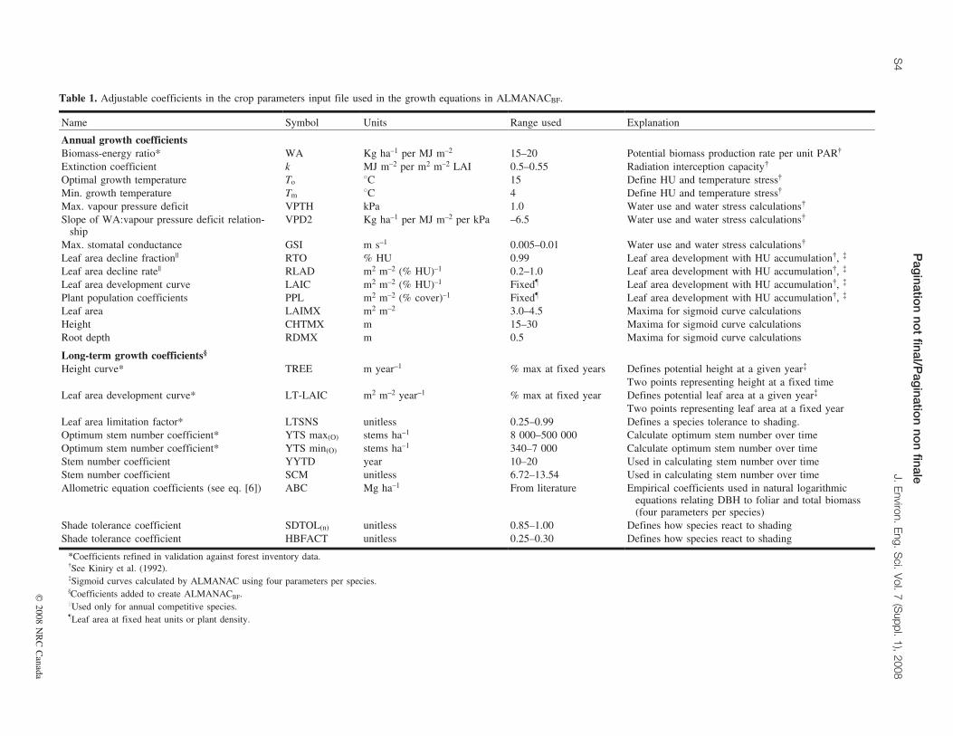
Table 1. Adjustable coefficients in the crop parameters input file used in the growth equations in ALMANACBF.

Name Symbol Units Range used Explanation

Annual growth coefficientsBiomass-energy ratio* WA Kg ha–1 per MJ m–2 15–20 Potential biomass production rate per unit PAR{

Extinction coefficient k MJ m–2 per m2 m–2 LAI 0.5–0.55 Radiation interception capacity{

Optimal growth temperature To 8C 15 Define HU and temperature stress{

Min. growth temperature Tm 8C 4 Define HU and temperature stress{

Max. vapour pressure deficit VPTH kPa 1.0 Water use and water stress calculations{

Slope of WA:vapour pressure deficit relation-ship

VPD2 Kg ha–1 per MJ m–2 per kPa –6.5 Water use and water stress calculations{

Max. stomatal conductance GSI m s–1 0.005–0.01 Water use and water stress calculations{

Leaf area decline fraction|| RTO % HU 0.99 Leaf area development with HU accumulation{, {

Leaf area decline rate|| RLAD m2 m–2 (% HU)–1 0.2–1.0 Leaf area development with HU accumulation{, {

Leaf area development curve LAIC m2 m–2 (% HU)–1 Fixed} Leaf area development with HU accumulation{, {

Plant population coefficients PPL m2 m–2 (% cover)–1 Fixed} Leaf area development with HU accumulation{, {

Leaf area LAIMX m2 m–2 3.0–4.5 Maxima for sigmoid curve calculationsHeight CHTMX m 15–30 Maxima for sigmoid curve calculationsRoot depth RDMX m 0.5 Maxima for sigmoid curve calculations

Long-term growth coefficients§

Height curve* TREE m year–1 % max at fixed years Defines potential height at a given year{

Two points representing height at a fixed timeLeaf area development curve* LT-LAIC m2 m–2 year–1 % max at fixed year Defines potential leaf area at a given year{

Two points representing leaf area at a fixed yearLeaf area limitation factor* LTSNS unitless 0.25–0.99 Defines a species tolerance to shading.Optimum stem number coefficient* YTS max(O) stems ha–1 8 000–500 000 Calculate optimum stem number over timeOptimum stem number coefficient* YTS min(O) stems ha–1 340–7 000 Calculate optimum stem number over timeStem number coefficient YYTD year 10–20 Used in calculating stem number over timeStem number coefficient SCM unitless 6.72–13.54 Used in calculating stem number over timeAllometric equation coefficients (see eq. [6]) ABC Mg ha–1 From literature Empirical coefficients used in natural logarithmic

equations relating DBH to foliar and total biomass(four parameters per species)

Shade tolerance coefficient SDTOL(n) unitless 0.85–1.00 Defines how species react to shadingShade tolerance coefficient HBFACT unitless 0.25–0.30 Defines how species react to shading

*Coefficients refined in validation against forest inventory data.{See Kiniry et al. (1992).{Sigmoid curves calculated by ALMANAC using four parameters per species.§Coefficients added to create ALMANACBF.||Used only for annual competitive species.}Leaf area at fixed heat units or plant density.

Pag

ination

not

final/Pag

ination

non

finale

S4

J.E

nviron.E

ng.S

ci.V

ol.7

(Suppl.

1),2008

#2008

NR

CC

anada

½2� RATIOm ¼ LAIm � km � expð��m � LAIHFmÞXni¼1

ðLAIi � ki � expð��i � LAIHFiÞÞ

where LAI and k are defined above, � is the weighted ex-tinction coefficient for the entire canopy above the halfheight of individual species, and LAIHF represents the sumof leaf area above the half height of individual species. Theexpression for RATIO indicates the PAR reaching an indivi-dual plant species is reduced exponentially by the extinctionof light caused by the canopy above it.

Multi-year growth algorithmsTree growth was included in the original ALMANAC

model to simulate its impact on the growth of understoreyperennials and annuals (Kiniry 1998). Consequently, therewas no real description of a ‘‘forest’’ per se. The ALMA-NACBF edition, includes (1) a general description of thetrees in a forest stand, including stem number (number oftrees), diameter at breast height (DBH), and foliar biomass;(2) an algorithm to account for variable productivity of indi-vidual forest sites; and (3) an algorithm that shifts the com-petitive advantage between the different species that aregrowing on the site to simulate forest successional change.

Forest stand descriptionThe first change that was made to ALMANAC was the

addition of a sigmoid curve to describe maximum annualleaf area and increase in plant height over the life of the for-est. We then incorporated a site-specific input parameter(SFTLAI) that shifts the position on the multi-year leaf areadevelopment curve to modify the potential LAI in year 1after disturbance. The long-term sigmoid curve is mathe-matically the same as annual sigmoid curves in ALMANAC(Kiniry et al. 1992), with the exception that the time scale isexpressed in years rather than degree days. Sigmoid curvesgenerated by ALMANAC are forced through the origin andtwo selected points using eq. [3]:

½3� F ¼ X

X þ expðy1� y2� XÞ

where the fraction (F) is a function of a time dependent fac-tor (X). The model generates the equation from two pairs ofinput values of F and X. For example, annual leaf area inputconsists of two values indicating percentage total leaf area(F) at two corresponding values of GDD (X). Parameters y1and y2 are generated by a curve fit within the model tothese two input points (Kiniry et al. 1992).

To calculate stem number (the number of trees), we de-veloped an attenuated exponential decay curve that was fitto Alberta Phase 3 Forest Inventory data for each tree spe-cies (eq. [4]).

½4� STMXi ¼ ðYTSmaxi � YTSminiÞ � 0:02ðY � YYTDiÞ� �2 � exp

Y � YYTDi

SCMi

� �� þ YTSmini

where for species ‘‘i’’, STMXi is the maximum number ofstems per hectare in a given year, YTS maxi and YTS miniare the maximum and minimum number of stems per hec-tare reported in forest inventory yield tables, respectively, Yis the year after stand establishment, YYTDi is the initialyear of stem number decline and SCMi is a species-specificcrop parameter that defines the steepness of the exponentialdecrease in stem number after stand establishment. TheSTMXi is constant until canopy closure (year YYTDi) andthen decreases exponentially. In ALMANACBF, the userspecifies the values for YTS max, YTS min, and YYTD fora species and ensures that Y ‡ YYTD. On this basis, themodel calculates standard decreases in stem number withstand maturity.

Average diameter at breast height for a tree species(DBHi) is back calculated for species ‘‘i’’ in the forest standusing species-specific allometric equations (Ter-Mikaelianand Korzukhin 1997) (eq. [5]):

½5� DBHi ¼AVBTi

ABC1i

� �ABC2i

where for species ‘‘i’’, AVBTi is the average biomass pertree expressed as biomass per hectare/STMAi, STMAi is thenumber of trees (stems) per hectare, and ABC1i and ABC2iare coefficients relating biomass to DBHi. Foliar biomass(FOLi in eq. [6] is then calculated using an additional allo-metric equation based upon the simulated DBHi.

Net annual above ground biomass production (NPP) for aspecific species ‘‘i’’ is calculated by subtracting losses of an-nual FOLi and annual stem loss from gross annual produc-tion (GPP) for species ‘‘i’’ (eq. [6]).

½6� NPPi ¼ GPPi � FOLi

��ðSTMLYAi � STMAiÞ � AVBTi

�where STMLYAi is stem number for species ‘‘i’’ from theprevious year, and STMAi and AVBTi are as defined above.

Height growth follows a sigmoid curve, but is limited bythe RATIO of intercepted PAR for each individual species.In this manner, height is synchronized with biomass. Themodel selects the dominant shading species (i.e., the speciesthat receives the largest fraction of PAR due to its heightand occupation in the canopy). For this species, heightgrowth is not limited. The dominant shading species is iden-tified using eq. [7]:

½7� HTMODMAX

¼ MAXi¼1 to n

HTMODi ¼ RATIOi �LAIMAXi

LAIPCi

� �

where HTMODi is the RATIO of PAR intercepted by spe-cies 1 to n and normalized by the ratio of the maximum po-tential LAI of the species (LAIMAXi) at 100% cover to the


MacDonald et al. S5

# 2008 NRC Canada

LAI at the percent cover defined by the user in the input file(LAIPCi).

It is important to assure that the height increment is re-duced proportional to the PAR-RATIO, and not due to therelative proportion that the species occupies in the canopy,as defined by the input chosen for the site. Therefore, dailyheight increments of all other species are reduced by theRATIO of PAR received by each species normalized by theratio of LAIMAXi to LAIPCi (eq. [8]):

½8� HTINCRAi

¼ HTINCRPiHTMODi

HTMODMAX � SDTOLi

� �HBFACTi

where HTINCRAi is the actual daily height increment forspecies ‘‘i’’ corrected for the effect of shading, HTINCRPiis the potential height increment calculated as a function ofthe ideal sigmoid height growth curve, HTMODi andHTMODMAX are defined as above, and SDTOLi andHBFACTi are species-specific plant parameters that definehow individual species react to shading. The factor SDTOLiallows species ‘‘i’’ to tolerate a certain amount of shadingwithout reducing height growth to account for species thatmaintain investment in height growth (Perry 1994) whenshaded to the detriment of diameter growth. As SDTOLi de-creases, species ‘‘i’’ will tolerate a certain amount of shad-ing without reducing height growth. The factor HBFACTiaccounts for variable allocations of biomass to diametergrowth because certain species will invest less biomass inheight growth and more in diameter and leaf area growth(Pothier and Prevost 2002; King 2005).

Variable site productivityGenerally, as the productivity of a forest site decreases,

the stem number increases, while DBH, height, and woodvolume (consequently biomass) decrease. These empiricalobservations are incorporated into typical yield tables thatindicate variable productivity (Plonski 1974). To simulatevariable site productivity, we used a similar approach tothat used in the TRIPLEX model (Bossel 1996; Peng et al.2002). ALMANACBF calculates stem number directly fromsite-specific input data. The DBH is back calculated from si-mulated biomass, and foliar biomass is calculated from spe-cies-specific allometric equations based on the simulatedDBH. As stem number increases, the DBH decreases pro-portionally. Consequently, since allometric equations are ex-ponential relationships between DBH and foliar biomass, thefoliar biomass of individual trees decreases exponentially.We assume that as foliar biomass decreases, LAI is reducedproportionally.

The model calculates foliar biomass for a given site pro-ductivity class. In parallel, the model calculates an optimumfoliar biomass based on the ‘‘optimum’’ stem number (op-timum stem number is a species-specific parameter). The ac-tual LAI (LAIPCA) for species ‘‘i’’ that is used to calculatespecies growth is then estimated with eq. [9]:

½9� LAIPCAi ¼ LAIPCi

BFOLSIi

BFOLSIOi

� �

where the maximum potential LAIPC for species ‘‘i’’ at agiven percent cover is reduced by the ratio of foliar biomass

at the site (BFOLSIi) to the optimum foliar biomass (BFOL-SIOi) at a good site with lower stem density and higherDBH trees. Using this simple approach, productivity is re-duced proportionally to allometric differences in trees at dif-ferent stand densities.

Successional changes in species dominationFinally, we incorporated an algorithm that describes suc-

cessional transitions from one plant type to another duringforest growth after disturbance. The transitions are based onshading in the understorey. As the height and leaf area ofthe upper canopy increases, the area available to shorter spe-cies with adequate light to grow becomes limited, and there-fore their frequency of occurrence will decrease (Lieffersand Stadt 1994). As canopy height increases, annual poten-tial LAI for shorter members of the vegetation cover is lim-ited by a species-specific factor (LAILIMm) according toeq. [10]:

½10� LAILIMm ¼ ðHTm � LAIPmÞXni¼1

ðHTi � LAIPiÞ

26664

37775LTSNSm

where LTSNSm is a species-specific factor that defines howa species reacts to shading, HTm and HTi are the heights ofspecies ‘‘m’’ and ‘i’’, respectively, and LAIPm and LAIPi arethe maximum leaf areas attained by species ‘‘m’’ and ‘i’’ inthe previous year, respectively. The factor LAILIMm definesthe maximum potential leaf area that species ‘‘m’’ can reachunder a given canopy.

Parameter summaryTo adapt ALMANACBF to forest growth, we incorporated

a total of 19 parameters under seven categories (Table 1).Most parameters can be found in current scientific literatureor were derived from yield tables, with some parameters likethe sigmoid growth curves, fit to forest inventory data. TheALMANACBF input file was modified to include YTS maxand YTS min and SFTLAI, the factor that modifies potentialLAI in year 1 after disturbance (harvesting). The input forthe sigmoid curve is the current year and the factor SFTLAIis added to the current year. Consequently a SFTLAI factorof 3 will result in the potential leaf area in year 1 after dis-turbance being equivalent to year 4 on the standard curve.

Material and methods

Site descriptionThe ALMANACBF model was developed to address the

complexities of Boreal Plain forests. A comprehensive de-scription of this region of the Boreal Plain is provided inSmith et al. (2003). Briefly, the annual precipitation is 300to 625 mm per year. The relief is flat to gently sloping. Up-land soils are predominantly deep, silty clay luvisols, formedon calcareous deposits with some occurrence of courser tex-tured, more acidic brunisols on glacio-fluvial and glacio-al-luvial deposits. Shallow aquifers exist due to impermeablelayers in glacial deposits resulting in occurrences of organicsoils and gleysols.



# 2008 NRC Canada

The forest structure is complex and mixed forest standsare very common. Dry upland stands are typically rapidlygrowing, consisting of pure lodgepole pine (Pinus contortaDougl. ex Loud. var. latifolia Engelm.), pure trembling as-pen (Populus tremuloides Michx.), and mixed trembling as-pen–lodgepole pine. Richer moist sites have pure whitespruce (Picea glauca (Moench) Voss), pure deciduous(trembling aspen and balsam poplar (Populusbalsamifera L.), and mixed spruce – deciduous stands – fir(Abies sp.). Wetlands and sites with organic soils are pre-dominantly slow growing pure black spruce (Picea mariana(Mill.) BSP) and mixed black spruce – deciduous – Larch(Larix sp.) stands (Beckingham and Archibald 1996).Data sources for model simulations

Most of the input data were obtained from existing publicsources, for example measurements for the Whitecourt, Al-berta weather station from 1984 to 2001 (Environment Can-

ada 2007). However, climate data for 2001 to 2004 wereobtained from a meteorological station located 40 km north-west of Whitecourt, maintained by the Forest Watershed andRiparian Disturbance (FORWARD) project in the MillarWestern Forest Products Ltd. forest management agreement(FMA) area. Data consisted of daily precipitation, maximumand minimum temperature, solar radiation, wind speed, andrelative humidity.

The Agricultural Region of Alberta Soil Inventory Data-base (AGRASID 2001) provided soil parameters requiredfor model simulations. These data consisted of saturated hy-draulic conductivity, bulk density, and water holding charac-teristics for each horizon of each soil series observed inAlberta. For all simulations in this article, one soil type wasused, a common orthic gray luvisol, with silty loam texture(Hubalta series), the dominant soil series in the Millar West-ern FMA area.

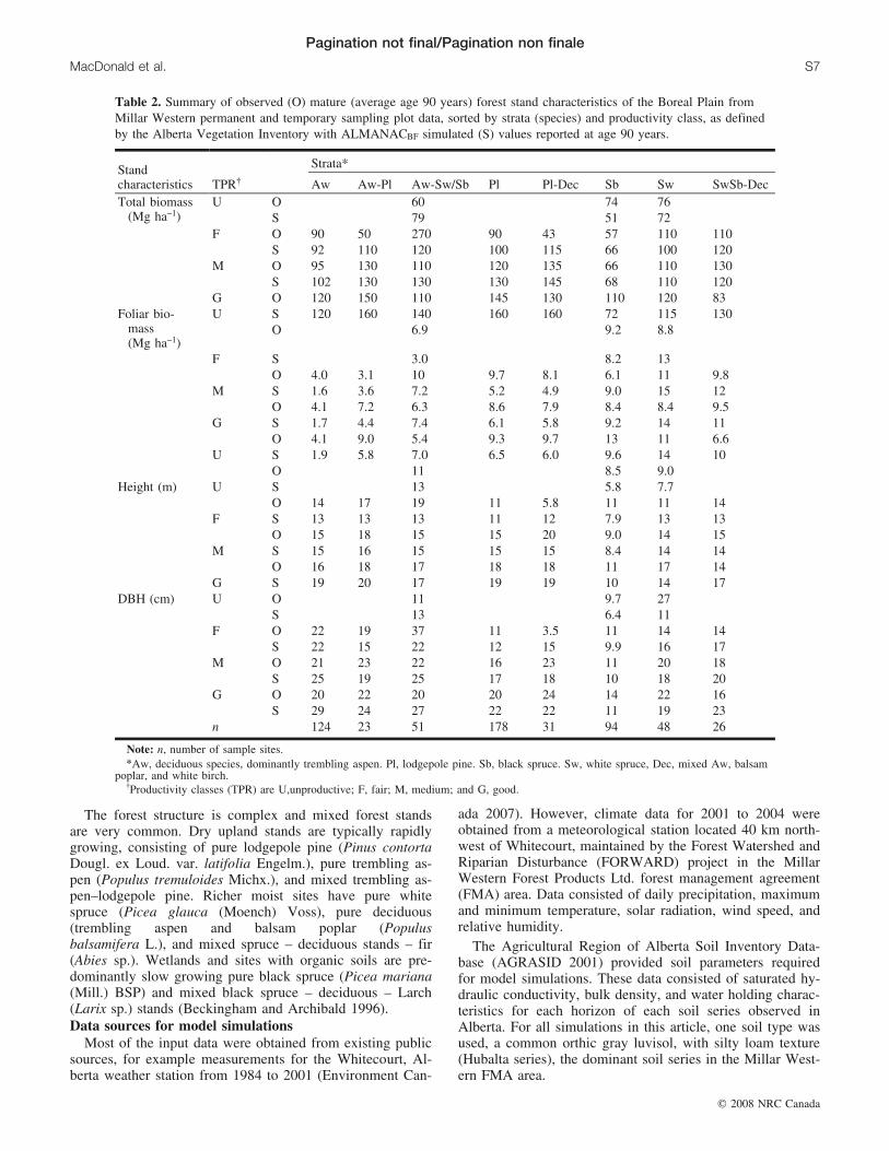
Table 2. Summary of observed (O) mature (average age 90 years) forest stand characteristics of the Boreal Plain fromMillar Western permanent and temporary sampling plot data, sorted by strata (species) and productivity class, as definedby the Alberta Vegetation Inventory with ALMANACBF simulated (S) values reported at age 90 years.

Standcharacteristics TPR{

Strata*

Aw Aw-Pl Aw-Sw/Sb Pl Pl-Dec Sb Sw SwSb-DecTotal biomass

(Mg ha–1)U O 60 74 76

S 79 51 72F O 90 50 270 90 43 57 110 110

S 92 110 120 100 115 66 100 120M O 95 130 110 120 135 66 110 130

S 102 130 130 130 145 68 110 120G O 120 150 110 145 130 110 120 83

Foliar bio-mass(Mg ha–1)

U S 120 160 140 160 160 72 115 130O 6.9 9.2 8.8

F S 3.0 8.2 13O 4.0 3.1 10 9.7 8.1 6.1 11 9.8

M S 1.6 3.6 7.2 5.2 4.9 9.0 15 12O 4.1 7.2 6.3 8.6 7.9 8.4 8.4 9.5

G S 1.7 4.4 7.4 6.1 5.8 9.2 14 11O 4.1 9.0 5.4 9.3 9.7 13 11 6.6

U S 1.9 5.8 7.0 6.5 6.0 9.6 14 10O 11 8.5 9.0

Height (m) U S 13 5.8 7.7O 14 17 19 11 5.8 11 11 14

F S 13 13 13 11 12 7.9 13 13O 15 18 15 15 20 9.0 14 15

M S 15 16 15 15 15 8.4 14 14O 16 18 17 18 18 11 17 14

G S 19 20 17 19 19 10 14 17DBH (cm) U O 11 9.7 27

S 13 6.4 11F O 22 19 37 11 3.5 11 14 14

S 22 15 22 12 15 9.9 16 17M O 21 23 22 16 23 11 20 18

S 25 19 25 17 18 10 18 20G O 20 22 20 20 24 14 22 16

S 29 24 27 22 22 11 19 23n 124 23 51 178 31 94 48 26

Note: n, number of sample sites.*Aw, deciduous species, dominantly trembling aspen. Pl, lodgepole pine. Sb, black spruce. Sw, white spruce, Dec, mixed Aw, balsam

poplar, and white birch.{Productivity classes (TPR) are U,unproductive; F, fair; M, medium; and G, good.


MacDonald et al. S7

# 2008 NRC Canada

Temporary and permanent sample plot dataForest data were obtained for the area surrounding the

FORWARD research watersheds (Smith et al. 2003; Prepaset al. 2006). Temporary (TSP) and permanent sample plot(PSP) data were collected in the FMA area between 1996and 2004 and consisted of 853 individual plots coveringstand ages from 5 years after disturbance to old growthstands as old as 180 years. Detailed descriptions of TSP andPSP vegetation data and detailed methodology on forest plotmeasurements are available elsewhere (The ForestryCorp. 1998; Millar Western Forest Products 2004). Briefly,each tree in a 100 m2 (TSP) or 400 m2 (PSP) plot was clas-sified according to species, height, height to live crown,DBH, crown class (position in the canopy ranked by heightwhether, dominant, co-dominant, intermediate, or sup-pressed), crown development, age (dominant trees werecored), lean, and tree quality.

The Alberta Vegetation Inventory (AVI) (Alberta Envi-ronmental Protection 1996) was used to differentiate the for-ested landscape into individual forest stands throughout theFMA area. The forest stands were differentiated into eightindividual strata based on the dominant species in the domi-nant storey. Information obtained from the AVI for dataanalysis and modelling was strata, site productivity class,and ecosite classification. Additional information was pro-vided by Millar Western regarding forest stands that hadbeen harvested since the development of the forest inven-tory. Stand age for each polygon within the geographic in-formation system database was taken from the AVI andsupplemented with harvest data. All information was re-ceived from Millar Western in the form of a geographicallyreferenced database that had each attribute required to set upmodel input files associated with each polygon within theFMA area.

We summarized the detailed individual tree measurementsbased on crown class only using the trees that were presentin actual forest canopies (i.e., dominant, co-dominant, andintermediate trees). Contributions of suppressed trees to totaland foliar biomass were insignificant (<10%). Total and fo-liar biomass was calculated using allometric equations (Ter-Mikaelian and Korzukhin 1997). Biomass per hectare wascalculated as the stem number per hectare of each crownclass times the average biomass from the average crownclass DBH. The height and DBH of each tree species in theplot was weighted based on number of stems and the aver-age height per canopy class. Individual plot data were sum-marized based on stand strata from AVI polygons and ageclass defined by 10-year intervals.

Results

Characteristics of Boreal Plain forest standsThe TSP and PSP data provided a general overview of the

characteristics of the forests of this region. Eight strata couldbe clearly defined, four of which represented mixed stands(Table 2). In general, late juvenile and mature forest stratathat had not entered into the old growth stage (stands from55 to 125 years of age) increased in total biomass, totalheight, and DBH in the following order: black spruce (Sb),deciduous species (mainly trembling aspen (Aw)), whitespruce (Sw), SwSb–Dec (Dec refers to mixed Aw, balsam

poplar and white birch (Betula papyrifera Marsh.)), Aw–SwSb, Aw–lodgepole pine (Pl), Pl–Dec, Pl. Mixed standswere generally more productive than pure stands of thedominant species occurring in a mixture. Foliar biomass in-creased in the following order: Aw, Aw–SwSb, Aw–Pl, Pl–Dec, SwSb–Dec, Sb, Pl, Sw. This demonstrates a gradientwith increased deciduous plants in mixed forests represent-ing the lower biomass to leaf area ratio of deciduous foliage.Overall productive sites (Good sites) were 35%, 35%, 25%,and 17% greater in biomass, height, foliar biomass, andDBH, respectively, than fair sites and 92%, 80%, 16%, and70% greater in biomass, height, foliar biomass, and DBH,respectively, than unproductive sites.

Model parameterizationALMANACBF was developed so that the characteristics of

the simulated trees could be compared to data that are col-lected by forestry companies in their TSP and PSP samplingprograms. To refine the growth parameters for trees in themodel, we worked with a subset of the TSP and PSP data.Selecting only pure stands of Aw (n = 51), Pl (n = 55), Sb(n = 60), and Sw (n = 42) and summarizing the TSP andPSP data by age class, we created a chronosequence ofheight and biomass.

We refined the biomass energy ratio (WA), leaf area de-velopment curve (LAIC), maximum height (CHTMX), andthe initial and final stem numbers (YTS max(O) andYTS min(O)) (Table 1) iteratively until we had the best fit tothe observed data, judged by a linear regression with thehighest r2 for total biomass, foliar biomass, height, andDBH (Table 3). In previous work (MacDonald et al. 2005),we refined coefficients related to seasonal parameters(height partitioning coefficients, seasonal heat unit relation-ships). We retained these parameters and a standard set ofphysiological parameters (Table 1) throughout all simula-tions.

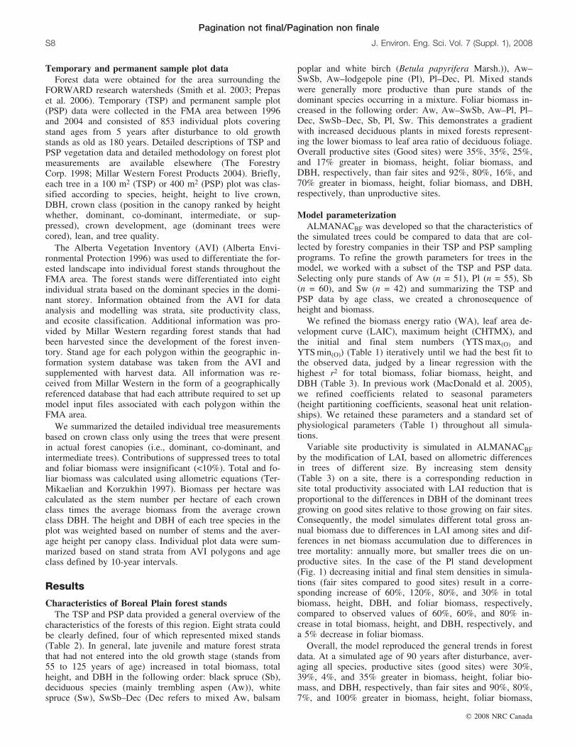
Variable site productivity is simulated in ALMANACBFby the modification of LAI, based on allometric differencesin trees of different size. By increasing stem density(Table 3) on a site, there is a corresponding reduction insite total productivity associated with LAI reduction that isproportional to the differences in DBH of the dominant treesgrowing on good sites relative to those growing on fair sites.Consequently, the model simulates different total gross an-nual biomass due to differences in LAI among sites and dif-ferences in net biomass accumulation due to differences intree mortality: annually more, but smaller trees die on un-productive sites. In the case of the Pl stand development(Fig. 1) decreasing initial and final stem densities in simula-tions (fair sites compared to good sites) result in a corre-sponding increase of 60%, 120%, 80%, and 30% in totalbiomass, height, DBH, and foliar biomass, respectively,compared to observed values of 60%, 60%, and 80% in-crease in total biomass, height, and DBH, respectively, anda 5% decrease in foliar biomass.

Overall, the model reproduced the general trends in forestdata. At a simulated age of 90 years after disturbance, aver-aging all species, productive sites (good sites) were 30%,39%, 4%, and 35% greater in biomass, height, foliar bio-mass, and DBH, respectively, than fair sites and 90%, 80%,7%, and 100% greater in biomass, height, foliar biomass,



# 2008 NRC Canada

Table 3. Input parameters for ALMANACBF derived through optimization and used throughout simulations.

Parameter description Source

Input parameters and variations

YYTD YTS G M F UStand population

descriptionOptimized with biomass,

height and DBH chronose-quence, TSP/PSP data

Aw 10 max 14 000 28 000 38 000 38 000

min 500 590 700 1050Pl 20 max 16 000 30 000 69 000 114 000

min 550 820 1200 2690Sb 20 max 56 000 100 000 120 000 200 000

min 2300 2400 2500 5000Sw 20 max 16 000 20 000 24 000 200 000

min 540 750 1080 2000

Orthic gray luvisol, Hubalta series, common Boreal Plain glacial till soil (silty loam)Soil input AGRASID (2001) Texture % Clay 11–36

Saturated conductivity (mm h–1) 10–100Water holding capacity (% volume) 8–10Coarse fragment (%) 0–18

Tree input parameters Optimized from TSP/PSP bio-mass ratios

Aw-SwSb (percent cover) 70% Aw 30% Sw

Aw-Pl (percent cover) 80% Aw 20% PlPl-Dec (percent cover) 50% Pl 50% Aw

Grouping of Ecosite classifications into three categoriesEcosite category Broad estimate from literature Xeric 40% Annual 40% shrub SFTLAI-0

Mesic 70% Annual 70% shrub SFTLAI-0Sub-hygric 100% Annual 100% shrub SFTLAI-2

Pag

ination

not

final/Pag

ination

non

finale

MacD

onaldet

al.S

9

#2008

NR

CC

anada

and DBH, respectively, than unproductive sites. Simulatedstands increased in total biomass, total height, and DBH inthe order: Sb, Aw, Sw, Aw–SwSb, SwSb–Dec, Pl, Aw–Pl,and Pl–Dec. As was the case in the observed data, simulatedmixed stands were generally more productive than purestands of the dominant species present in a mixture. Thehigher productivity of the mixed stands is a result of thenon-linear (sigmoid) relationship between the percent coverin the input file, and the LAI (parameters PPL in Table 1).Consequently in mixed stands, the potential LAI for thecombined species was slightly elevated relative to a purestand. Foliar biomass increased in the order Aw, Aw–Pl,

Pl–Dec, Aw–SwSb, Pl, Sb, SwSb–Dec, and Sw, demonstrat-ing a gradient with increased deciduous plants in mixed for-ests representing the lower biomass to leaf area ratio ofdeciduous foliage.

Understorey vegetationAcross the three ecozones in the Millar Western FMA

area, there are approximately 50 ecosite classifications. Intheoretical simulations (described in more detail below), wevaried the percent cover (equivalent to the seeding rate forannual crops), as well as the factor SFTLAI, which modifiesthe sigmoid curve controlling potential LAI change with

Fig. 1. ALMANACBF simulations of variable growth in different productivity classes of Lodgepole Pine Stands. (a) Stand biomass. (b) Standheight. (c) Diameter at breast height (DBH). (d) Foliar biomass. Comparison to observed means in TSP/PSP data from stands ranging from55 to 125 years of age.

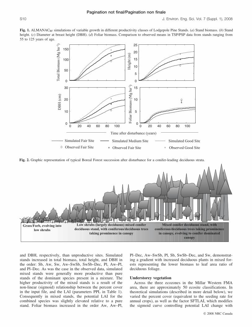
Fig. 2. Graphic representation of typical Boreal Forest succession after disturbance for a conifer-leading deciduous strata.



# 2008 NRC Canada

time (Table 3). A fixed plant growth parameter (mass car-bon per unit energy input) for generic perennial grasses andforbs that have an annual growth cycle was set at 1.2 g CMJ–1 with a maximum potential LAI of 5.0, when fully es-tablished at 100% cover and a maximum height of 1 m. Afixed parameter for deciduous shrubs was set at 1.7 g CMJ–1 with a maximum potential LAI of 3.5, when fully es-tablished at 100% cover and a maximum height of 3.5 m.

Based on these input parameters, we simulated variations inannual biomass production that ranged from 0.22 to 1.5 Mgha–1 in ‘‘xeric’’ sites compared to 3 to 3.7 Mg ha–1 in thesimulated ‘‘sub-hygric’’ sites. The model does not simulatethe extremes reported in the literature; however with simplemodification of input parameters, the model is very capableof providing a reasonable simulation of differences in pro-ductivity.

Successional changes in forests: Leaf area index and lightinterception

While TSP and PSP data provide an idea of the type ofstands that exist on the forest landscape, those forests havepassed through a process of succession to arrive at theirpresent forest structure. A typical growth trajectory in theboreal forest involves successional changes in plant speciescomposition (Fig. 2). Immediately after disturbance, the veg-etation covering the site is dominated by annual forbs andperennial grasses, evolving into low shrub cover. Aroundthe time of canopy closure, we observe a deciduous–conifer-ous tree and shrub canopy, evolving into a young mixed de-ciduous–coniferous forest and eventually, a mature forestdominated by large coniferous species or staying as a decid-uous overstorey. The forest strata (tree species), ecosite, andsite productivity determine how the site will evolve.

In ALMANACBF model simulations, the combination ofthe light partitioning equations (eqs. [1] and [2]) with thelong-term leaf area development equation (eq. [3]) and thesuccessional equation that limits potential leaf area basedon species height and LAI in previous years (eq. [10]) de-scribe changes in LAI over the life of the stand. Leaf areais a fundamental parameter in hydrological modelling, be-cause it defines the area of a vegetative canopy that captureslight and intercepts rainfall.

Different combinations of crop tree species (strata) grow-ing in different ecosites (Figs. 3a to 3f) result in very differ-

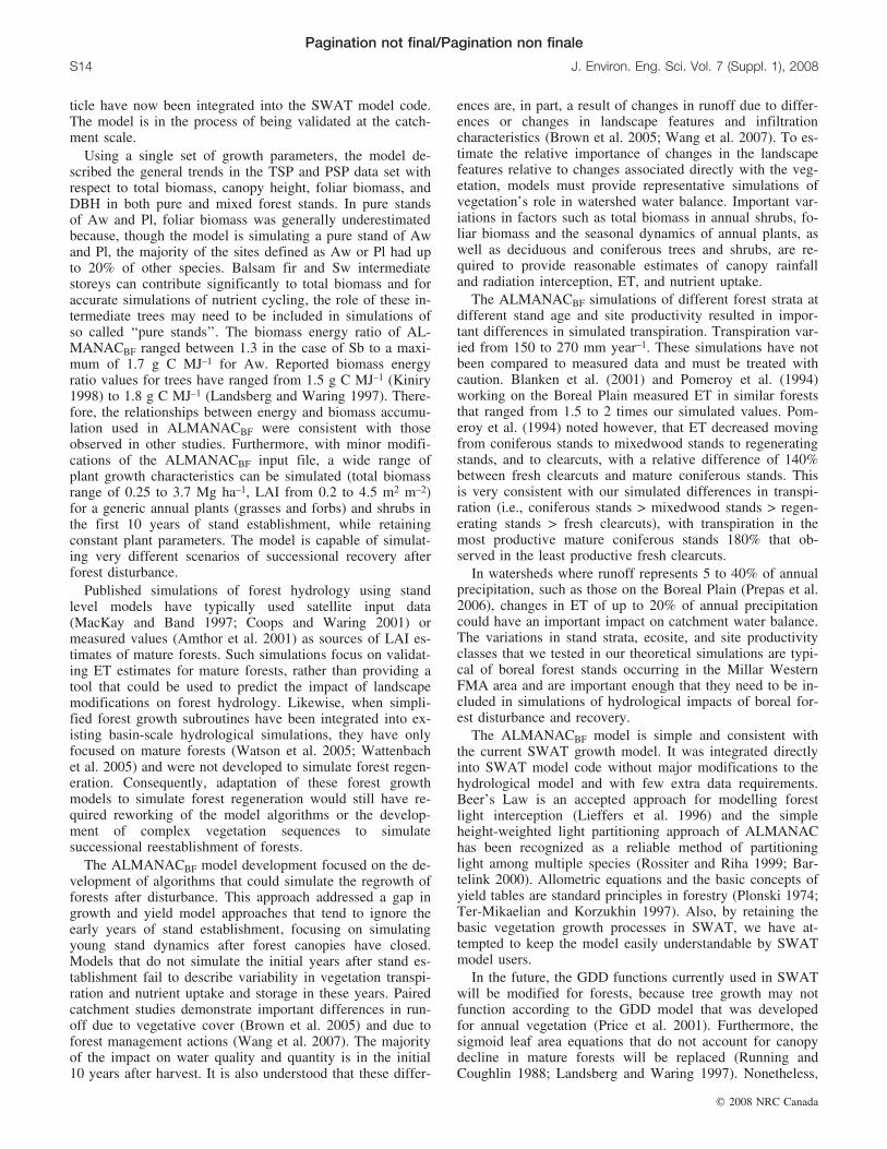
Fig. 4. ALMANACBF simulations of photosynthetically active ra-diation (PAR) interception in: (a) mixed white spruce (Sw)-aspen(Aw) sub-hygric ecosite; (b) mixed lodgepole pine (Pl)-Aw xericecosite.

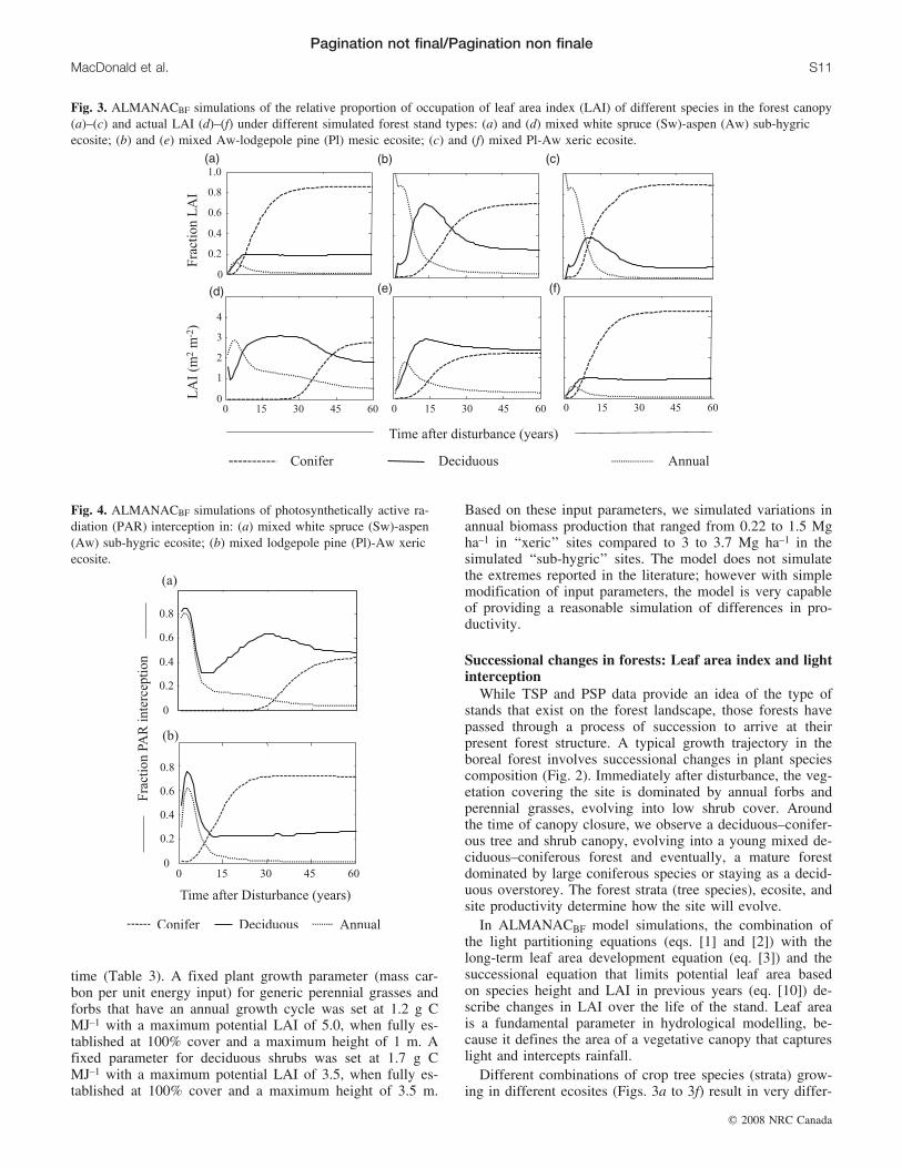
Fig. 3. ALMANACBF simulations of the relative proportion of occupation of leaf area index (LAI) of different species in the forest canopy(a)–(c) and actual LAI (d)–(f) under different simulated forest stand types: (a) and (d) mixed white spruce (Sw)-aspen (Aw) sub-hygricecosite; (b) and (e) mixed Aw-lodgepole pine (Pl) mesic ecosite; (c) and (f) mixed Pl-Aw xeric ecosite.


MacDonald et al. S11

# 2008 NRC Canada

ent growth trajectories as represented by changes in LAIwith time after disturbance. In the years immediately afterdisturbance, annual (i.e., grasses and forbs) plants dominatedthe canopy in all scenarios, but were reduced to 10% of thetotal canopy (0.3–0.5 m2 m–2) over the first 20 to 40 years.In conifer-dominated stands (Figs. 3a and 3c), deciduousspecies dominated the forest canopy from 5 years after dis-turbance to 15 or 50 years, depending on the rate of conifergrowth; pine species rapidly dominating the forest canopy(20–30 years) and spruce developing slowly (40–50 years).In aspen-dominated stands (Fig. 3b), coniferous speciesgradually established a secondary canopy. Each simulatedstrata varied in the period that deciduous, conifer, and an-nual species dominated the forest canopy.

While the proportions of the LAI were dependent on spe-cies combinations, the absolute values of LAI were depend-ent on ecosite and site productivity. In the xeric-sub-mesicsite, leaf area developed slowly over the first 5 to 10 years(0.17 in year 1, 1.3 in year 5, 2.3 m2 m–2 in year 10),whereas it developed rapidly on the hygric site (3.7 in year1, 4.4 in year 5, 4.4 in year 10) and rapidly reached a max-imum in year 8 (Figs. 3d to 3f).

Light interception was partitioned among the differentspecies using the simple PAR partitioning model describedby Kiniry et al. (1992). In general, PAR interception wasproportional to LAI development (Figs. 4a to 4b). However,as tree species established their canopy over the shrub andannual species, the proportion of light allotted to the annualplant and shrub species was decreased relative to their pro-portion of the LAI (eq. [2]). At 50 years after disturbance,annuals maintained an LAI that is 10 to 15% of total canopybut receive only 5 to 10% of total PAR.

Biomass partitioningThe concept of RUE is used to convert PAR to biomass.

Biomass is partitioned among the different species based on

the distribution of LAI (Fig. 3) and the PAR intercepted byeach individual species (Fig. 4). Consequently, the propor-tional changes in biomass are similar to changes observedin the relative proportion of LAI and PAR interception.However, from the perspective of hydrological transportmodelling, it is the distribution of biomass among differentplant types that is important, because the model must pro-vide a reasonable estimate of biomass that is returned to theforest floor in the form of litter and also nutrients that arestored in plant tissues for the long term. The use of speciesspecific allometric equations (eq. [5]) allows an estimate offoliar tissue to be derived by back-calculating DBH from thetotal biomass.

Among different combinations of mixed forests (Fig. 5),foliar biomass also follows the same pattern as LAI andPAR interception with a transformation from an annual spe-cies dominated canopy, to deciduous cover to an eventualconiferous contribution. The exception in the case of foliarbiomass is the disproportionately large biomass of coniferousfoliage per unit leaf area relative to deciduous foliage. As aconsequence, even in sites that are dominated by deciduoustrees with respect to leaf area, coniferous foliage rapidlycomes to occupy the largest proportion of foliar biomass.

As was the case with LAI, variability was seen in the realvalues of foliar biomass observed with the input associatedwith ecosite classification (Figs. 5d to 5f). In simulated sub-hygric sites, annual foliar biomass ranged from 3 to5 Mg ha–1 in the first 10 years after disturbance comparedto only 1 to 1.5 Mg ha–1 in the case of the simulated xericsite.

Changes in evapotranspirationThe ALMANACBF model calculates ET using the Pen-

man-Monteith equation and simulated water uptake exactlyas does the SWAT model, assuming EPCO (the parameterdefining the distribution of water uptake from soil horizons)

Fig. 5. ALMANACBF simulations of the relative proportion of total foliar biomass of different species in the forest canopy of a forest re-generating after disturbance (a)–(c) under different forest trajectories and foliar biomass (d)–(f). Stand types include: (a) and (d) mixedwhite spruce (Sw)-aspen (Aw) sub-hygric ecosite; (b) and (e) mixed Aw-lodgepole pine (Pl) mesic ecosite; (c) and (f) mixed Pl-Aw xericecosite.



# 2008 NRC Canada

is 1.0 (Kiniry et al. 1992; Neitsch et al. 2002). As calculatedby the Penmen-Monteith equation, transpiration is influ-enced only by plant parameters, height and LAI and is lim-ited by plant water availability. Simulated variations inspecies and ecosite result in changes in transpiration thatproduce important variations in simulated seasonal transpira-tion throughout the age of the stand (Figs. 6a to 6c). Themost important differences indicated by the simulationswere (1) the more productive sites, with greater potentialLAI, had roughly 20% greater transpiration than xeric–poorsites in the first year after disturbance (Fig. 6a); (2) transpi-ration increased by as much as 40% (Fig. 6b) from year 1 toa peak beginning in the middle of the growth cycle (64 yearsof age); (3) in the transition from juvenile stands (age 36) tomature stands (age 64) annual transpiration differed by asmuch as 55% among Aw, Sw, and Pl strata (Fig. 6c);

(4) seasonal differences among conifer, annual, and decidu-ous species were evident, with roughly 20% of total annualtranspiration occurring in early spring in coniferous standsbefore deciduous and annual canopies were established(Figs. 6b and 6c); and (5) an increase in stand productivityresulted in an increase of about 14% in the annual total oftranspiration (Aw fair site productivity to Aw good site pro-ductivity) (Fig. 6c).

Discussion and conclusions

ALMANACBF is intended to provide a generic descriptionof variability in forest growth, with very little informationabout individual sites. The simulations presented here werecarried out using the soil, water, and nutrient subroutines inALMANAC, but the model algorithms described in this ar-

Fig. 6. ALMANACBF simulations of cumulative annual evapotranspiration in a theoretical forest site using the Penman-Monteith equationwith constant weather input data. (a) Year 1 after disturbance varying maximum site LAI to simulate ecosites spanning the edatopic grid,varying from rich, hygric sites (moist, nutrient rich sites) to xeric, poor sites (dry nutrient poor sites). (b) Sw–Aw strata at different agesduring the growth trajectory. (c) ET in juvenile and mature forests, different strata, different site productivity.



# 2008 NRC Canada

ticle have now been integrated into the SWAT model code.The model is in the process of being validated at the catch-ment scale.

Using a single set of growth parameters, the model de-scribed the general trends in the TSP and PSP data set withrespect to total biomass, canopy height, foliar biomass, andDBH in both pure and mixed forest stands. In pure standsof Aw and Pl, foliar biomass was generally underestimatedbecause, though the model is simulating a pure stand of Awand Pl, the majority of the sites defined as Aw or Pl had upto 20% of other species. Balsam fir and Sw intermediatestoreys can contribute significantly to total biomass and foraccurate simulations of nutrient cycling, the role of these in-termediate trees may need to be included in simulations ofso called ‘‘pure stands’’. The biomass energy ratio of AL-MANACBF ranged between 1.3 in the case of Sb to a maxi-mum of 1.7 g C MJ–1 for Aw. Reported biomass energyratio values for trees have ranged from 1.5 g C MJ–1 (Kiniry1998) to 1.8 g C MJ–1 (Landsberg and Waring 1997). There-fore, the relationships between energy and biomass accumu-lation used in ALMANACBF were consistent with thoseobserved in other studies. Furthermore, with minor modifi-cations of the ALMANACBF input file, a wide range ofplant growth characteristics can be simulated (total biomassrange of 0.25 to 3.7 Mg ha–1, LAI from 0.2 to 4.5 m2 m–2)for a generic annual plants (grasses and forbs) and shrubs inthe first 10 years of stand establishment, while retainingconstant plant parameters. The model is capable of simulat-ing very different scenarios of successional recovery afterforest disturbance.

Published simulations of forest hydrology using standlevel models have typically used satellite input data(MacKay and Band 1997; Coops and Waring 2001) ormeasured values (Amthor et al. 2001) as sources of LAI es-timates of mature forests. Such simulations focus on validat-ing ET estimates for mature forests, rather than providing atool that could be used to predict the impact of landscapemodifications on forest hydrology. Likewise, when simpli-fied forest growth subroutines have been integrated into ex-isting basin-scale hydrological simulations, they have onlyfocused on mature forests (Watson et al. 2005; Wattenbachet al. 2005) and were not developed to simulate forest regen-eration. Consequently, adaptation of these forest growthmodels to simulate forest regeneration would still have re-quired reworking of the model algorithms or the develop-ment of complex vegetation sequences to simulatesuccessional reestablishment of forests.

The ALMANACBF model development focused on the de-velopment of algorithms that could simulate the regrowth offorests after disturbance. This approach addressed a gap ingrowth and yield model approaches that tend to ignore theearly years of stand establishment, focusing on simulatingyoung stand dynamics after forest canopies have closed.Models that do not simulate the initial years after stand es-tablishment fail to describe variability in vegetation transpi-ration and nutrient uptake and storage in these years. Pairedcatchment studies demonstrate important differences in run-off due to vegetative cover (Brown et al. 2005) and due toforest management actions (Wang et al. 2007). The majorityof the impact on water quality and quantity is in the initial10 years after harvest. It is also understood that these differ-

ences are, in part, a result of changes in runoff due to differ-ences or changes in landscape features and infiltrationcharacteristics (Brown et al. 2005; Wang et al. 2007). To es-timate the relative importance of changes in the landscapefeatures relative to changes associated directly with the veg-etation, models must provide representative simulations ofvegetation’s role in watershed water balance. Important var-iations in factors such as total biomass in annual shrubs, fo-liar biomass and the seasonal dynamics of annual plants, aswell as deciduous and coniferous trees and shrubs, are re-quired to provide reasonable estimates of canopy rainfalland radiation interception, ET, and nutrient uptake.

The ALMANACBF simulations of different forest strata atdifferent stand age and site productivity resulted in impor-tant differences in simulated transpiration. Transpiration var-ied from 150 to 270 mm year–1. These simulations have notbeen compared to measured data and must be treated withcaution. Blanken et al. (2001) and Pomeroy et al. (1994)working on the Boreal Plain measured ET in similar foreststhat ranged from 1.5 to 2 times our simulated values. Pom-eroy et al. (1994) noted however, that ET decreased movingfrom coniferous stands to mixedwood stands to regeneratingstands, and to clearcuts, with a relative difference of 140%between fresh clearcuts and mature coniferous stands. Thisis very consistent with our simulated differences in transpi-ration (i.e., coniferous stands > mixedwood stands > regen-erating stands > fresh clearcuts), with transpiration in themost productive mature coniferous stands 180% that ob-served in the least productive fresh clearcuts.

In watersheds where runoff represents 5 to 40% of annualprecipitation, such as those on the Boreal Plain (Prepas et al.2006), changes in ET of up to 20% of annual precipitationcould have an important impact on catchment water balance.The variations in stand strata, ecosite, and site productivityclasses that we tested in our theoretical simulations are typi-cal of boreal forest stands occurring in the Millar WesternFMA area and are important enough that they need to be in-cluded in simulations of hydrological impacts of boreal for-est disturbance and recovery.

The ALMANACBF model is simple and consistent withthe current SWAT growth model. It was integrated directlyinto SWAT model code without major modifications to thehydrological model and with few extra data requirements.Beer’s Law is an accepted approach for modelling forestlight interception (Lieffers et al. 1996) and the simpleheight-weighted light partitioning approach of ALMANAChas been recognized as a reliable method of partitioninglight among multiple species (Rossiter and Riha 1999; Bar-telink 2000). Allometric equations and the basic concepts ofyield tables are standard principles in forestry (Plonski 1974;Ter-Mikaelian and Korzukhin 1997). Also, by retaining thebasic vegetation growth processes in SWAT, we have at-tempted to keep the model easily understandable by SWATmodel users.

In the future, the GDD functions currently used in SWATwill be modified for forests, because tree growth may notfunction according to the GDD model that was developedfor annual vegetation (Price et al. 2001). Furthermore, thesigmoid leaf area equations that do not account for canopydecline in mature forests will be replaced (Running andCoughlin 1988; Landsberg and Waring 1997). Nonetheless,



# 2008 NRC Canada

the model algorithms outlined in this article that simulatepartitioning of light and biomass among species and biomasswithin species, as well as the simple procedures to simulatesuccession of a stand overtime, are promising. Furthermore,the model algorithms take advantage of all useful site-spe-cific information that can be derived from data available atthe landscape scale in foresters’ geographically referenceddatabases.

AcknowledgementsDuring this study, the FORWARD project was funded by

the Natural Sciences and Engineering Research Council ofCanada (CRD and Discovery Grants to E.E. Prepas), theCanada Foundation for Innovation, Millar Western ForestProducts Ltd., Blue Ridge Lumber Inc. (a division of WestFraser Mills Ltd.), Vanderwell Contractors (1971) Ltd.,ANC Timber Ltd., the Living Legacy Research Program,and the Ontario Innovation Trust. In particular, we wish tothank Jonathan Russell (Millar Western) and Daryl D’Amico(Blue Ridge Lumber). ALMANAC, like SWAT, is availablefrom the United States Department of Agriculture free ofcost. Documentation, code and example data sets can be ob-tained from Dr. Jim Kiniry and Dr. Jeff Arnold.

ReferencesAGRASID. 2001. Agricultural region of Alberta Soil Inventory Da-

tabase (AGRASID). Version 3.0 [online] Agriculture Food andRural Development, Edmonton, Alta. Available from www.agric.gov.ab.ca/$department/deptdocs.nsf/all/sag3249Alberta[cited 20 February 2001].

Alberta Environmental Protection. 1996. Alberta Vegetation Inven-tory Standards Manual. Final Draft Version 2.2 (July). AlbertaEnvironmental Protection, Resource Data Division, Data Acqui-sition Branch, Edmonton, Alta.

Aldred, A.H. 1981. A federal/provincial program to implementcomputer-assisted forest mapping for inventory and updating.Dendron Resource Surveys Ltd., Ottawa, Ont.

Allen, R.G., Jensen, M.E., Wright, J.L., and Burman, R.D. 1989. Op-erational estimates of evapotranspiration. Agron. J. 81: 650–662.

Amthor, J.S., Chen, J.M., Clein, J.S., Frolking, S.E., Goulden,M.L., Grant, R.F., Kimball, J.S., King, A.W., McGuire, A.D.,Nikolov, N.T., Potter, C.S., Wang, S., and Wofsy, S.C. 2001.Boreal forest CO2 exchange and evapotranspiration predicted bynine ecosystem process models: Intermodel comparisons and re-lationships to field measurements. J. Geophys. Res. 106: 33623–33648. doi:10.1029/2000JD900850.

Arnold, J.G., Srinivasan, R., Muttiah, R.S., and Williams, J.R.1998. Large area hydrological modeling and assessment part I:model development. J. Am. Water Resour. Assoc. 34: 73–89.doi:10.1111/j.1752-1688.1998.tb05961.x.

Bartelink, H.H. 2000. A growth model for mixed forest stands. For.Ecol. Manage. 134: 29–43. doi:10.1016/S0378-1127(99)00243-1.

Beckingham, J.D., and Archibald, J.H. 1996. Field guide to ecositesof northern Alberta. Special Report 5. 528 pages, 88 photo-graphs, 88 botanical drawings, 24 figures, 1 large map. NaturalResources Canada, Canadian Forest Service, Northern ForestryCentre, Edmonton, Alta.

Blanken, P.D., Black, T.A., Neumann, H.H., den Hartog, G., Yang,P.C., Nesic, Z., and Lee, X. 2001. The seasonal water and en-ergy exchange above and within a boreal aspen forest. J. Hydrol.245: 118–136. doi:10.1016/S0022-1694(01)00343-2.

Bosch, J.M., and Hewlett, J.D. 1982. A review of catchment ex-

periments to determine the effect of vegetation changes on wateryield and evapotranspiration. J. Hydrol. 55: 3–23. doi:10.1016/0022-1694(82)90117-2.

Bossel, H. 1996. TREEDYN3 Forest Simulation Model. Ecol.Model. 90: 187–227. doi:10.1016/0304-3800(95)00139-5.

Brown, A.E., Zhang, L., McMahon, T.A., Western, A.W., and Ver-tessy, R.A. 2005. A review of paired catchment studies for de-termining changes in water yield resulting from alteration invegetation. J. Hydrol. 310: 28–61. doi:10.1016/j.jhydrol.2004.12.010.

Coops, N.C., and Waring, R.H. 2001. The use of multiscale remotesensing imagery to derive regional estimates of forest growth ca-pacity using 3-PGS. Remote Sens. Environ. 75: 324–334.doi:10.1016/S0034-4257(00)00176-0.

Decatanzaro, J.B., and Kimmins, J.P. 1985. Changes in the weightand nutrient composition of litter fall in three forest ecosystemtypes on coastal British Columbia. Botany, 63: 1046–1056.

Environment Canada. 2007. Digital archive of the Canadian clima-tological data (surface). Atmospheric Environment Service [on-line]. Canadian Climate Centre, Data Management Division,Downsview, Ont. Available from www.climate.weatheroffice.ec.gc.ca/ climateData/canada_e.html [cited 25 February 2001].

Farley, K.A., Jobbagy, E.G., and Jackson, R.B. 2005. Effects of af-forestation on water yield: a global synthesis with implicationsfor policy. Glob. Change Biol. 11: 1565–1576. doi:10.1111/j.1365-2486.2005.01011.x.

Kimmins, J.P., Mailly, D., and Seely, B. 1999. Modelling forestecosystem net primary production: the hybrid simulation ap-proach used in forecast. Ecol. Model. 122: 195–224. doi:10.1016/S0304-3800(99)00138-6.

King, D. 2005. Linking tree form allocation and growth with an al-lometrically explicit model. Ecol. Model. 185: 77–91. doi:10.1016/j.ecolmodel.2004.11.017.

King, K.W., and Balogh, J.C. 2001. Water quality impacts asso-ciated with converting farmland and forests to turfgrass. Trans.ASAE, 44: 569–576.

Kiniry, J.R. 1998. Biomass accumulation and radiation use effi-ciency of honey mesquite and eastern red cedar. Biomass Bioe-nergy, 15: 467–473. doi:10.1016/S0961-9534(98)00057-9.

Kiniry, J.R., Williams, J.R., Gassman, P.W., and Debaeke, P. 1992.A general, process-oriented model for two competing plant spe-cies. Trans. ASAE, 35: 801–810.

Landhausser, S.M., and Lieffers, V.J. 1998. Growth of Populus tre-muloides in association with Calamagrostis canadensis. Can. J.For. Res. 28: 396–401. doi:10.1139/cjfr-28-3-396.

Landsberg, J.J., and Waring, R.H. 1997. A generalised model offorest productivity using simplified concepts of radiation-use ef-ficiency, carbon balance and partitioning. For. Ecol. Manage.95: 209–228. doi:10.1016/S0378-1127(97)00026-1.

Lane, C.T., Willoughby, M.G., and Alexander, M.J. 2000. Rangeplant community types and carrying capacity for the LowerFoothills subregion of Alberta. Pub. No. T/532. Alberta Environ-ment and Alberta Agriculture Food and Rural Development. Ed-monton. Alta. 232 pp.

Lieffers, V.J., and Stadt, K.J. 1994. Growth of understory Piceaglauca, Calamagrostis canadensis, and Epilobium angustifoliumin relation to overstory light transmission. Can. J. For. Res. 24:1193–1198.

Lieffers, V.J., Macmillan, R.B., MacPherson, D., Branter, K., andStewart, J.D. 1996. Semi-natural and intensive silvicultural sys-tems for the boreal mixedwood forest. For. Chron. 72: 286–292.

MacDonald, J.D., Kiniry, J., Arnold, J., McKeown, R., Whitson, I.,Putz, G., and Prepas, E.E. 2005. Developing parameters to simu-late trees with SWAT. In Proceedings of the 3rd International



# 2008 NRC Canada

SWAT 2000 Conference, Zurich, Switzerland. Edited by K. Ab-baspour and R. Srinivasan. Texas Water Resources Institute,College Station, Tex.

MacKay, D.S., and Band, L.E. 1997. Forest ecosystem processes at thewatershed scale: Dynamic coupling of distributed hydrology andcanopy growth. Hydrol. Proc. 11: 1197–1217. doi:10.1002/(SICI)1099-1085(199707)11:9<1197::AID-HYP552>3.0.CO;2-W.

McKeown, R., Putz, G., Arnold, J., and Whitson, I. 2004. Stream-flow modelling in a small forested watershed on the Canadianboreal plain using a modified version of the soil and water as-sessment tool (SWAT). In Proceedings of the 1st Water and En-vironment Specialty conference of the Canadian Society forCivil Engineering. Saskatoon, Sask.

Millar Western Forest Products. 2004. Permanent sample plot man-ual. May 2004. Millar Western Forest Products Ltd., Whitecourt,Alta. 82 pp. plus appendices.

Miller, S.N., Kepner, W.G., Mehaffey, M.H., Hernandez, M., Miller,R.C., Goodrich, D.C., Devonald, K.K., Heggem, D.T., and Miller,W.P. 2002. Integrating landscape assessment and hydrologicmodeling for land cover change analysis. J. Am. Water Resour.Assoc. 38: 915–929. doi:10.1111/j.1752-1688.2002.tb05534.x.

Monteith, J.L. 1965. Evaporation and the environment. In Proceed-ings of the XIXth Symposium The State and Movement ofWater in Living Organisms, Society For Experimental Biology,Swansea. Cambridge University Press. pp. 205–234.

Neitsch, S.L., Arnold, J.G., Kiniry, J.R., Williams, J.R., and King,K.W. 2002. Soil and Water Assessment Tool: Theoretical Docu-mentation, version 2000. TWRI Report TR-191. Texas WaterResources Institute, College Station, Tex. 458 pp.

Peng, C., Liu, J., Dang, Q., Apps, M.J., and Hong, J. 2002. TRI-PLEX: a generic hybrid model for predicting forest growth andcarbon and nitrogen dynamics. Ecol. Model. 153: 109–130.doi:10.1016/S0304-3800(01)00505-1.

Perry, D. 1994. Forest ecosystems. Johns Hopkins University Press,Baltimore, Md. 649 pp.

Phillips, E.E. 1950. Heat summation theory as applied to canningcrops. The Canner, 27: 13–15.

Plonski, W.L. 1974. Normal yield tables (metric) for major forestspecies of Ontario. Ontario Ministry of Natural Resources, Tor-onto, Ont. 40 pp.

Pomeroy, J.W., Hedstrom, N., Dion, K., Elliott, J., and Granger,R.J. 1994. Quantification of Hydrological Pathways in thePrince Albert Model Forest. 1993–1994 Annual Report. NHRIContribution No. CS-94006. 76 pp.

Pothier, D., and Prevost, M. 2002. Photosynthetic light responseand growth analysis of competitive regeneration after partial cut-ting in a boreal mixed stand. Trees (Berl.), 16: 365–373.

Prepas, E.E., Burke, J.M., Whitson, I.R., Putz, G., and Smith, D.W.2006. Associations between watershed characteristics, runoff,and stream water quality: Hypothesis development for watersheddisturbance experiments and modelling in the Forest Watershedand Riparian Disturbance (FORWARD) project. J. Environ.Eng. Sci. 5(Suppl. 1): S27–S37. doi:10.1139/S05-033.

Price, D.T., Zimmermann, N.E., van der Meer, P.J., Lexer, M.J.,Leadley, P., Jorritsma, I.T.M., Shaber, J., Clark, D.F., Lasch, P.,McNulty, S., Wu, J., and Smith, B. 2001. Regeneration in gapmodels: Priority issues for studying forest responses to climatechange. Clim. Change, 51: 475–508. doi:10.1023/A:1012579107129.

Putz, G., Burke, J.M., Smith, D.W., Chanasyk, D.S., Prepas, E.E.,and Mapfumo, E. 2003. Modelling the effects of boreal forestlandscape management upon streamflow and water quality: Ba-sic concepts and considerations. J. Environ. Eng. Sci. 2(Suppl. 1): S87–S101. doi:10.1139/s03-032.

Rossiter, D.G., and Riha, S.J. 1999. Modeling plant competitionwith the GAPS object-oriented dynamic simulation model.Agron. J. 91: 773–783.

Running, S.W., and Coughlin, J.C. 1988. General model of forestecosystem processes for regional applications, hydrological bal-ance, canopy gas exchange and primary production processes.Ecol. Model. 42: 125–154. doi:10.1016/0304-3800(88)90112-3.

Sahin, V., and Hall, M.J. 1996. The effects of afforestation and de-forestation on water yields. J. Hydrol. 178: 293–309. doi:10.1016/0022-1694(95)02825-0.

Saleh, A., Williams, J.R., Wood, J.C., Hauck, L.M., and Blackburn,W.H. 2004. Application of APEX for forestry. Trans. ASAE, 47:751–765.

Smith, D.W., Prepas, E.E., Putz, G., Burke, J.M., Meyer, W.L., andWhitson, I. 2003. The forest watershed and riparian disturbancestudy: A multi-disciplinary initiative to evaluate and managewatershed disturbance on the Boreal Plain. J. Environ. Eng. Sci.2(Suppl. 1): S1–S13. doi:10.1139/s03-030.

Spitters, C.J.T., and Aerts, R. 1983. Simulation of competition forlight and water in crop–weed associations. Aspects Appl. Biol.4: 467–483.

Ter-Mikaelian, M.T., and Korzukhin, M.D. 1997. Biomass equa-tions for sixty-five North American tree species. For. Ecol. Man-age. 97: 1–24. doi:10.1016/S0378-1127(97)00019-4.

The Forestry Corp. 1998. Temporary Sample Plot Program: Proto-col and Establishment. The Forestry Corp., Edmonton, Alta. 30pp.

Titus, S.J. 1998. Adaptation of the Mixedwood Growth Model(MGM) to northeastern British Columbia. Final Report Contract#JV99–011. BC Ministry of Forests, Resources InventoryBranch.

Wang, J.R., Zhong, A.L., Comeau, P., Tsze, M., and Kimmins, J.P.1995. Aboveground biomass and nutrient accumulation in anage sequence of aspen (Populus tremuloides) stands in the Bor-eal White and Black Spruce Zone, British Columbia. For. Ecol.Manage. 78: 127–138. doi:10.1016/0378-1127(95)03590-0.

Wang, X., Saleh, A., McBroom, M.W., Williams, J.R., and Yin, L.2007. Test of APEX for nine forested watersheds in East Texas.J. Environ. Qual. 36: 983–995. doi:10.2134/jeq2006.0087.PMID:17526877.

Waring, R.H., and Running, S.W. 1998. Forest ecosystems: Analy-sis at multiple scales. 2nd ed. Academic Press, New York, NY.370 pp.

Watson, B.M., Coops, N., Ghafouri, M., and Selvalingam, S. 2005.Simulating leaf area index of eucalyptus forest and pine planta-tions for a catchment-scale water balance model. In Proceedingsof the 29th Hydrology and Water Resources Symposium. Can-berra, Australia.

Wattenbach, M., Hattermann, F., Weng, R., Wchsung, F., Krysa-nova, V., and Badeck, F. 2005. A simplified approach to imple-ment forest eco-hydrological properties in regional hydrologicalmodelling. Ecol. Model. 187: 40–59.

Wattenbach, M., Zebisch, M., Hattermann, F., Gottschalk, P., Goe-mann, H., Kreins, P., Badeck, F., Lasch, P., Suckow, F., andWechsung, F. 2007. Hydrological impact assessment of affores-tation and change in tree-species composition- A regional casestudy for the Federal State of Brandenburg (Germany). J. Hy-drol. 346: 1–17. doi:10.1016/j.jhydrol.2007.08.005.

Welham, C., Seely, B., and Kimmins, H. 2002. The utility of thetwo pass harvesting system: an analysis using the ecosystem si-mulation model FORECAST. Can. J. For. Res. 32: 1071–1079.doi:10.1139/x02-029.

Willoughby, M.G. 2000. Guide to range plant communities andcarrying capacity for the Dry and Central Mixedwood subre-



# 2008 NRC Canada

gions of Alberta. Pub. no. T/526. Alberta Environment and Al-berta Agriculture Food and Rural Development, Edmonton,Alta. 187 pp.

Willoughby, M.G. 2005. Range plant communities and carrying ca-pacity for the Upper Foothills. Pub. no. T/003. Alberta Environ-ment and Alberta Agriculture Food and Rural Development,Edmonton, Alta. 138 pp.

List of symbols

ABC1i,ABC2i

species-specific plant parameter. Coefficients usedin allometric equations relating biomass to DBH(unitless).

AVBTi internal model-calculated coefficient. Average bio-mass per tree calculated as biomass per hectareover stem number per hectare (Mg tree–1).

BFOLSIi foliar biomass for an individual tree at the inputproductivity class calculated with allometric equa-tions (kg tree–1).

BFOLSIOi foliar biomass for an individual tree at a good siteat lower stem density and higher DBH trees(kg tree–1).

DBHi average breast height diameter for a tree species(m).

EPCO SWAT model parameter defining the distribution ofwater uptake from soil horizons (unitless).

ET evapotranspiration (mm).FOLi foliar biomass (Mg ha–1).

FRAC-TION(PAR)

internal model-calculated coefficient. Fraction ofPAR intercepted by the complete canopy (unitless).

GDD growth degree days (8C days).GPP gross primary productivity (Mg ha–1 year–1).

HBFACTi species specific plant parameter. Defines how indi-vidual species react to shading to calculated heightgrowth (unitless).

HTi, HTm calculated output. Height of an individual species(m).

HTIN-CRAi

internal model-calculated coefficient. Actual dailyheight increment corrected for the effect of shading(m).

HTINCR-Pi

internal model calculated coefficient. Potentialheight increment calculated as a function of theideal sigmoid height growth curve (m).

HTMODi internal model calculated coefficient. Ratio of PARintercepted by species 1 to n, normalized by the ra-tio of the maximum potential LAI of the species at100% cover to the potential LAI at the cover inputby the user (unitless).

HTMOD-MAX

internal model-calculated coefficient. Value for themaximum ratio of PAR intercepted by the dominantspecies in the input array (unitless)

HU heat units.ki, km species-specific plant parameter. Light extinction

coefficients as defined by Beer’s Law (unitless).LAIi,LAIm

calculated output. Leaf area index (m2 m–2).

LAIHFi,LAIHFm

internal model-calculated coefficient. Value of thecombined leaf area index above half the height of aspecies within the array of modelled species (m2 m–2).

LAILIMi internal model-calculated coefficient. Factor limit-ing leaf area development for understorey species(unitless).

LAIMAXi species specific plant parameter. Leaf area index at100% cover (m2 m–2).

LAIPi,LAIPm

internal model-calculated coefficient. Maximum an-nual leaf area of a species in the year previous tothe current year (m2 m–2).

LAIPCi internal model calculated coefficient. Species leafarea index at the percent cover defined by the userin the input file (m2 m–2).

LAIPCAi internal model-calculated coefficient. Species actualleaf area index corrected for site productivity index(m2 m–2).

LTSNSm species-specific plant parameter. Defines how aspecies reacts to shading in calculating leaf arealimitation in understorey (unitless).

i, m, n subscripts to designate a species in an array of spe-cies (i.e., species 1 through n).

NPP net primary productivity (Mg ha–1 year–1).RATIOi,RATIOm

internal model-calculated coefficient. Relative pro-portion of PAR that a species intercepts taking intoaccount shading (unitless).

RUEi species-specific plant parameter. Radiation use effi-ciency (Kg MJ–2).

SCMi species-specific plant parameter. Defines the expo-nential decrease in stem number after stand estab-lishment (unitless).

SDTOLi species-specific plant parameter. Defines how indi-vidual species react to shading to calculate heightgrowth (unitless).

SFTLAI site specific input. Shifts the multi-year leaf areadevelopment curve depending on the ecosite classi-fication (year).

STMAi calculated output. Stem number in the current year(stems ha–1).

STMLYAi internal model-calculated coefficient. Stem numberfrom the previous year (stems ha–1).

STMXi internal model-calculated coefficient. Maximumnumber of stems per hectare for a species(stems ha–1).

VPD vapour pressure deficit. Difference between theamount of moisture in the air and how much moist-ure the air can hold when saturated (kPa).

Y internal model calculation. The year after stand es-tablishment (year).

YTS maxi site specific input. Maximum number of stems re-ported in yield tables that is associated with a pro-ductivity class (stems ha–1).

YTS mini site-specific input. Minimum number of trees re-ported in yield tables (stems ha–1).

YYTDi species-specific plant parameter. The first year thatstem number begins to decline (year).

�i, �m internal model-calculated coefficients. Theweighted extinction coefficient of the combined ca-nopy above half the height of a species within thearray of modelled species (unitless).



# 2008 NRC Canada

A multi-species, process based vegetation simulation ...

Documents

Transcript of A multi-species, process based vegetation simulation ...