A Model for Window Based Flow Control Packet-Switched

Networks

by

Xiaowei Yang

Submitted to the Department of Electrical Engineering and ComputerScience

in partial fulfillment of the requirements for the degree of

Master of Science

at the

MASSACHUSETTS INSTITUTE OF TECHNOLOGY

March 1998

@ Massachusetts Institute of Technology 1998. All rights reserved.

Author ..... . ...................... . .. . . . . .. . . . .

Department of Electrical Engineering and Computer ScienceMarch 6th, 1998

Certified by . ... . . . . . ..' .. .... . . . . . . .- .. . . . . . . . . . . .. . . . . . . . . . .

Dr. David D. ClarkSenior Research Scientist, Laboratory for Computer Science

Thesis Supervisor

Accepted by ............ ............Arthur C. Smith

Chairman, Departmental Committee on Graduate Students

uf K K ..r~~'" '

A Model for Window Based Flow Control Packet-Switched Networks

by

Xiaowei Yang

Submitted to the Department of Electrical Engineering and Computer Scienceon January 5th, 1998, in partial fulfillment of the

requirements for the degree ofMaster of Science

Abstract

Recently, networks have increased rapidly both in scale and speed. Problems related tothe control and management are of increasing interest. However, there is no satisfactorytool to study the behavior of such networks. The traditional event driven simulation isslow when the network speed is high. The time driven simulation is against the nature ofpacket-switched networks. As Transmission Control Protocol (TCP) is the most widelyused transport layer protocol, and it uses window based flow control mechanism, classicqueuing theories involving Markov Chain assumptions are not applicable.

This thesis develops a model for the window based flow control packet-switched net-works. The model attempts to provide a way to study large and high speed networks usingTCP. In this thesis, we discuss in detail the construction, implementation and application ofthe model. This thesis also compares the results obtained from the model with those fromthe packet by packet event driven simulation. The comparison shows the model is correctlymodeling the networks.

Thesis Supervisor: Dr. David D. ClarkTitle: Senior Research Scientist, Laboratory for Computer Science

I

Acknowledgments

I would like to thank my thesis advisor, Dave Clark, for his advice and support. I appreciate

his kindness to give me a chance to study in the field of networking. I also appreciate his

intuition and patience which helped me go through this project. I thank Karen Sollins and

John Wroclawski for their help whenever I ran into problems.

I thank the system administrator of ANA group, Dorothy Curtis, who spent a lot of

time in setting up my computers, installing software I need and answering all my questions

about UNIX.

I thank Prof. Robert Gallager and Dr. Balaji Prabhakar, who are lecturers of Data

Communication Networks. Not only has their class greatly enriched my knowledge of

networking but also the advice I got from them helped me gain some insight into this

project.

I thank my friends Li-wei Lehman, Dina Katabi and my former officemate Ulana Leg-

edza, for their generous share of knowledge and their encouragement. I also thank Prof.

Lixia Zhang for her guidance through emails and her kindness to help me.

I thank the people in the ANA group: Rob Cheng, Wenjia Fang, Lewis Girod, Mark

Handley, Daniel Lee, Atanu Mukherjee, Alex C. Snoeren, Elliot Schwartz, Rena Yang.

They are always valuable resources to find an answer to any question.

I thank my advisor of my undergraduate study at Tsinghua University, Deyun Lin.

Without his recommendation, I may not have the chance to come to MIT.

I thank my family in China. Though they are far alway from me, the telephone con-

versations with them and their letters give me the strength to overcome all difficulties I

face.

Finally, but by no means less important, I sincerely thank Daniel Jiang, for his dedicated

love and care.

Contents

1 Introduction

1.1 Motivation ...................................

1.2 Organization of this Thesis . .........................

2 Related Work

2.1 Simulation Methods ..............................

2.2 Queuing Theories .......................

2.3 Summary ...................................

3 Model Construction

3.1 End-to-end Window Based Flow Control . ..................

3.2 Basic Assumptions . . . . .............................

3.3 The Model ...................................

4 Algorithm

4.1 The Difficult Point ..............

4.2 How to Find a Solution for the Model . . . .

4.2.1 Ideas . . . . . . . . . . . . ....

4.2.2 D etails . . . . . . . . . . . . . . . .

4.2.3 Another Perspective of the Algorithm

4.3 Short Discussion About the Implementation

27

. . . . . . . . . . . . . .. . 2 8

. . . . . . . . . . . . . . . . 30

. . . . . . . . . . . . . . .. 30

. . . . . . . . . . . . . . . . 30

. . . . . . . . . . . . . . . . 3 3

. . . . . . . . . . . . . . . . 35

5 Implementation Issues and Testing Results

5.1 How to Reduce the Number of Iterations . . . . . . . . . . . .

5.2 How to Solve the Equations in E(a) . ........... .. . .. . . 39

5.3 Performance Analysis ............................. 41

5.4 Results Comparison with those of ns ................... .. 42

5.4.1 A Brief Introduction of a Test Net . ................. 42

5.4.2 Results . . . . . . . . . . . . . . . . . . . . . . . . . . . . . . . . 42

6 Application Results 45

6.1 RED ....................................... 45

6.2 A ssum ptions ........... .. .. ..... ... ... . .. .. .. 46

6.3 The Event Driven Simulation ........... . . ........ . . 46

6.3.1 The Simulating Method ....................... 46

6.3.2 Results . . . . . . . . . . . . . . . . . . . . . . . . . . . . . . . . 48

6.4 The Time Driven Simulation ................... ...... 50

6.4.1 The Simulating Method ................ ....... 50

6.4.2 Results . . . . . . . . . . . . . . . . . . . . . . . . . . . . . . . . 52

7 Summary and Future Work 57

7.1 Sum m ary ... ........... ... . .. ........ . .. .... 57

7.2 Future W ork ... .... ..... .. .. ..... ...... ... . . .. 57

List of Figures

3-1 A simple illustrative example ..........

3-2 A general example ...............

How to recognize congested links: An example

N- C, a .. ................

N C, , a. . ................

Nk, Ck C' . ...............0kL J

..... .......... 22

.. .. .......... 25

. . . . . . . . . . . . . . . 29

..... .......... 33

...... ......... 34

..... .......... 35

5-1 A Redundant Constrain: (A1 + A2 < C3 ) . ..

Simulation Results of a Low Speed Net . . . . . . .

Simulation Results of a High Speed Net .......

Simulation Results of a Low Speed Net: At = 0.30s

Simulation Results of a High Speed Net: At = 0.25s

Simulation Results of a Low Speed Net: At = 0.50s

6-6 Simulation Results of a High Speed Net: At = 0.50s

. . . . . . . . . . 4 9

. . . . . . . . . . . . 4 9

. . . . . . . . . . . . 5 3

. . . . . . . . . . . . 5 4

. . . . . . . . . . . . 5 5

. . . . . . . . . . . . 5 5

4-1

4-2

4-3

4-4

6-1

6-2

6-3

6-4

6-5

10

List of Tables

4.1 Each flow's static round trip delay in Figure 4-1 . .............. 29

5.1 Results Comparison: Queue Lengths ................... .. 43

5.2 Results Comparison: Average rates of flows . ................ 43

12

Chapter 1

Introduction

1.1 Motivation

The Internet has been growing rapidly in recent years, which results in problems related to

routing, flow control, administration etc. Simulation and analysis are the two commonly

used methods to study the characteristics of networks. However, when networks become

very large, neither method is easy to implement. For example, the traditional packet by

packet level event driven simulation is slow when simulating a high speed network. The

fixed granularity of the event driven simulation is the bottleneck of its speed. Unless we

change the abstraction level, it is hard to improve its performance. Analytic method often

uses classic queuing and network stochastic models which are restricted to problems that

can be approximated as Markov chains [1]. As networks are using complicated protocols

such as TCP/IP to implement flow control, they can't be simply modeled by Markov chain

assumption. Thus, we lack a satisfying model to study the behavior of window based flow

control packet-switched networks.

The goal of this thesis is to develop a simple and applicable model for window based

flow control packet-switched networks under some reasonable assumptions. The model is

expected to ignore the packet-level behavior of networks. Instead, it gives a higher level

description, such as the average flow rate and the average queue length at each outgoing

link. Incorporating this model into simulation methods will hopefully provide a practical

way to study the behavior of large scale networks.

1.2 Organization of this Thesis

Chapter 2 is a review of the related work. Chapter 3 introduces the model. It includes basic

assumptions the model depends on and it also describes the meaning of every formula in

the model. Chapter 4 presents an algorithm for applying the model. Chapter 5 discusses

the implementation details. Chapter 6 shows how to apply this model to simulate TCP with

RED. The last chapter is a short summary of the thesis and an assessment of future work.

Chapter 2

Related Work

2.1 Simulation Methods

As networks become larger and more complex, more and more researchers are using sim-

ulation to conduct the study of networks. Two effective ways are used for network simu-

lation. One is the discrete event driven simulation. The other is the discrete time driven

simulation. Since in most networks, data are chopped into discrete packets, discrete event

driven simulation is straightforward and it often can grasp the nature of networks.

The current academic-wide popular network simulator, ns [3], developed by the Net-

work Research Group at Lawrence Berkeley National Laboratory(LBNL), is part of the

Virtual InterNetwork Testbed(VINT) project [2]. The goal of VINT is to build a network

simulator which will facilitate the study of scale and protocol interaction of modem net-

work protocols. ns is a discrete event driven simulator which can simulate a wide range of

protocols, such as TCP and other routing, multicast protocols. In this thesis, ns is used to

test the model.

The representation of an event in ns is the state of a packet. Typical events could be the

arrival or departure of a packet from a queue. Thus, detailed information of each packet's

behavior can be obtained via simulation. ns has a global scheduler which manages an event

queue. This queue is arranged in the time sequence that the events should happen. The

simulation proceeds by simulating each event in the order they are stored in the queue. As

one event takes place, it can trigger other events. These events are also inserted into the

queue based on the time they are to happen. For the packet level event driven simulation,

the simulator has to simulate each packet's behavior even if we are not interested in such a

fine abstraction level.

When the network's size is moderate, ns is an ideal tool to study network protocols. The

detailed information about each packet's trace, such as when the packet arrives at a specific

router, or when and where the packet is dropped, can be precisely recorded. However,

discrete event driven simulation is slow when the speed of networks is high. First, the

packet level granularity is fixed in spite of the size of the network. Second, in order to

update the effects caused by each event, the event order must be kept. A global event

list has to be maintained, which results in an essentially sequential process. These two

phenomena can not be avoided in the discrete event driven simulation.

A discrete time driven simulation updates the state of each simulated object at each

delta time interval. Choosing a proper time interval is always a difficult problem. If the time

interval is too large, the simulation will fail to detect events which should have occurred

during the time interval. If such events are significant, the simulation's error bar will be

high. On the contrary, as the simulator has to update the state of each simulated object at

each delta interval, if the delta interval is too small, the simulator has to do the updating

very frequently. If we have a large network which contains a lot of objects, since not every

object changes its state so frequently, the simulation is very ineffective. Especially when

we are interested in a long time period simulation, it may also take a long time to do so

many updatings.

Another proposal is to use fluid model based time-driven simulation to simulate high

speed networks [7]. This model simulates the network traffic as fluid. It is proved that the

discretization error can be bounded by a constant proportional to the discretization time

interval. This model can quickly locate the time and place of congestion. Besides, by the

nature of time driven simulation, parallelism can be exploited to speed up the simulation.

However, under what circumstance the network traffic can be modeled as fluid still needs

further study. In the window flow control network, the rates of flows are unknowns. The

fluid model needs the arrival rates of flows as input. We do not know whether the fluid

model is adequate enough to model the window based flow control networks.

2.2 Queuing Theories

Also, there are a lot of well developed queuing and stochastic network theories related to

network flow and congestion control. When the network is large, those analytic models tend

to contain some impractical assumptions such as Markov chain. Thus, it is not convenient

to apply such queuing theories to window flow control networks.

2.3 Summary

In a word, for large scale and high speed window flow control networks, there is no satisfy-

ing model. The task of this thesis is to construct an analytic model for such networks. We

will discuss it in the next chapter.

18

Chapter 3

Model Construction

This chapter describes the model for window based flow control networks. We first give

a brief overview of the end-to-end window based flow control mechanism that is used

by TCP. Next, we present an abstraction of the real TCP. Our model is applicable under

some assumptions. Since the network's steady state is the point of interest, omissions of

implementation details of TCP will not hurt the model's praticability.

3.1 End-to-end Window Based Flow Control

A flow of data between a sender A and a receiver B is said to be end-to-end window flow

controlled if there is an upper bound on the data units that have been sent by A but are not

known by A to have been received by B [I]. The upper bound is called window size. In

TCP, the upper bound is used both to keep the sender from overflowing the receiver's buffer

and to keep the sender from overflowing the buffers inside the network. The sender keeps

two window sizes for the two purposes. The congestion window reflects the congestion

condition in the network. When the network is under heavy congestion, by reducing the

congestion window size, the sender holds the data units from entering the network. The

advertised window tells the sender the available buffer size in the receiver's side. The

sender's real window size should never exceed either of them. TCP uses ACKs from the

receiver to inform the sender of the correct receipt of data packets. When there is a full

window size of packets on fly, the sender can not advance its window until it receives an

ACK from the receiver.

Window based flow control can not guarantee a minimum sending rate nor a minimum

packet delay. When the network is suffering congestion, packets are queued up inside the

network. It will take a packet a long time to go through the network. So does the ACK.

If the window size is fixed, the longer the delay is, the lower the throughput is. And if

there are many senders competing for the limited links' capacities, each sender can only

get a small transmitting rate. Thus packets are blocked in output links. The packet delay is

increased with the increase of waiting queues.

3.2 Basic Assumptions

Though window flow control does not guarantee rate and delay, in some circumstances, we

are still interested in knowing how much the average rates window-controlled flows could

achieve and how large the queue size could be at each outgoing link if each flow's window

size is known and fixed. Doing packet by packet level simulation is a way to find out those

parameters. However, simulation is usually time consuming. We aim at a simple model

which can provide us the steady state information fast and fairly accurately.

As we are interested only in the steady state, we want to give some assumptions to

clarify the situation we are studying.

* Network configurations: assume we know the topology of the network, each link's

capacity and propagation delay.

* Routing and Queuing Policy:

1. Assume fix route routing. All packets belonging to the same sender and receiver

travel through the same path. The routing table of each router is known.

2. Assume routers keep a distinct output queue for each outgoing link. The pro-

cessing delay of each packet at the router is negligible compared to the propa-

gation delay, queuing delay and transmission delay.

3. The output buffer is infinite. We do not consider buffer overflow for now.

4. All data packets are of the same priority class. They are all arranged into a

single queue and first come, first transmitted.

* Flows:

1. All flows have fixed window sizes, and the network is in a steady state, e.g.,

each flow has a full window size of packets on fly and the packets are spaced

evenly.

2. Senders always have data to send. In the period of our study, no flows stop

sending data and no new flows start sending.

3. There is only one-way traffic flow. When a receiver receives a data packet, it

sends an ACK back immediately. ACKs travel through the same paths as those

of their acked data packets'. Since ACKs are tiny packets, we assume ACKs

are never backlogged at any link's output queue.

* Packets: All packets are of the same length. In this thesis, we assume the packet

length is 1 Kbyte.

In the next section, we discuss our model based on the above assumptions.

3.3 The Model

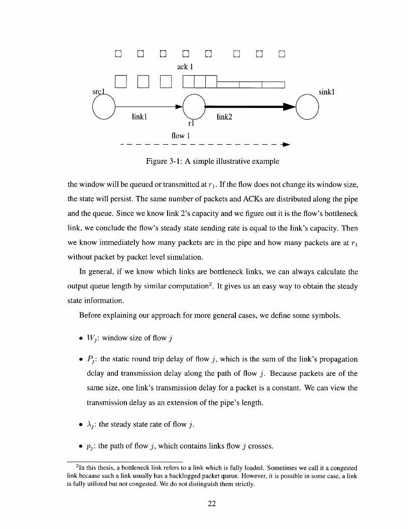
We start from a simple example to get some intuition. Figure 3-1 shows the example. There

is only one sender which is sending with a window size W. By the network's steady state

assumption, the flow has W packets on fly. They are either inside the pipe, transmitted by

srcl or ri or be queued at rl. Since the flow is sending packets evenly spaced, the number

of packets in the pipe is roughly (t + t2 ) (A denotes the flow's rate, e.g., the number of

packets the flow sends per unit time). t1 , t 2 are link 1 and 2's propagation delay. And the

number of returning ACKs is also - + . If link 2 is the bottleneck link, the other packets in

This assumption is not necessary. It only means to simplify programming. If ACKs travel throughsymmetric paths as those of data packets, only the forwarding paths of data packets need to be specified. Themodel is also applicable when ACKs travel through asymmetric paths. The only difference is we have tospecify both data and ACKs' paths in order to calculate the round trip delay.

F-r r-I r- ri rI r-1 r- r-LJ LJ LJ LJ LJ LJ LJ LJ

ack 1

src sinkl

link1 link2rl

flow 1-- - - - - - - - - - - - - - - - - -0

Figure 3-1: A simple illustrative example

the window will be queued or transmitted at rl. If the flow does not change its window size,

the state will persist. The same number of packets and ACKs are distributed along the pipe

and the queue. Since we know link 2's capacity and we figure out it is the flow's bottleneck

link, we conclude the flow's steady state sending rate is equal to the link's capacity. Then

we know immediately how many packets are in the pipe and how many packets are at rl

without packet by packet level simulation.

In general, if we know which links are bottleneck links, we can always calculate the

output queue length by similar computation2 . It gives us an easy way to obtain the steady

state information.

Before explaining our approach for more general cases, we define some symbols.

* Wj: window size of flow j

* P: the static round trip delay of flow j, which is the sum of the link's propagation

delay and transmission delay along the path of flow j. Because packets are of the

same size, one link's transmission delay for a packet is a constant. We can view the

transmission delay as an extension of the pipe's length.

* A : the steady state rate of flow j.

* p3 : the path of flow j, which contains links flow j crosses.

2In this thesis, a bottleneck link refers to a link which is fully loaded. Sometimes we call it a congestedlink because such a link usually has a backlogged packet queue. However, it is possible in some case, a linkis fully utilized but not congested. We do not distinguish them strictly.

* Ni: number of backlogged packets at outgoing link i. If the link i is a congested link,

Ni > 0. Otherwise, Ni = 0.

* nji: number of backlogged packets from flow j at link i. If the link i is a congested

link, n., > 0. Otherwise, nji = 0.

* C: capacity of link i.

According to the assumptions, we have:

For a flow j,P

W,- + nji (3.1)A3 iEp,

For a link i,

Ni = nji (3.2)jEi

Nevertheless, in a general case, we usually do not know each flow's steady state's send-

ing rate. In fact, it is an unknown we want to compute. Thus, from Equation 3.1 and 3.2,

we can not easily get nj nor N. However, Aj and n3i are related. They satisfy a set of

physical constraints. The extra constraints provide a way to find out rates of flows and

queue lengths at congested links.

As we know, if link i is not congested,

njz = 0, Vj Ei (3.3)

Ni = 0 (3.4)

If link i is congested, the link must be sending at its full capacity. So,

Ci = Aj (3.5)jEi

If link i is not congested,

Cz > : A (3.6)jEi

In the steady state, if a link i is congested, each flow j across link i has a constant

number of packets queued at it. The more backlogged packets one flow has at link i's output

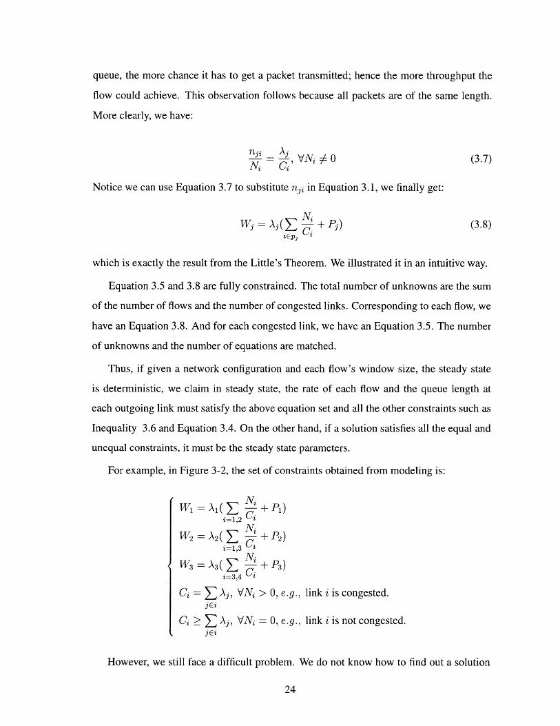
queue, the more chance it has to get a packet transmitted; hence the more throughput the

flow could achieve. This observation follows because all packets are of the same length.

More clearly, we have:

n= , VN 0 (3.7)Ni C'

Notice we can use Equation 3.7 to substitute nji in Equation 3.1, we finally get:

Niwj = Aj( (Z + P j ) (3.8)

iEp j

which is exactly the result from the Little's Theorem. We illustrated it in an intuitive way.

Equation 3.5 and 3.8 are fully constrained. The total number of unknowns are the sum

of the number of flows and the number of congested links. Corresponding to each flow, we

have an Equation 3.8. And for each congested link, we have an Equation 3.5. The number

of unknowns and the number of equations are matched.

Thus, if given a network configuration and each flow's window size, the steady state

is deterministic, we claim in steady state, the rate of each flow and the queue length at

each outgoing link must satisfy the above equation set and all the other constraints such as

Inequality 3.6 and Equation 3.4. On the other hand, if a solution satisfies all the equal and

unequal constraints, it must be the steady state parameters.

For example, in Figure 3-2, the set of constraints obtained from modeling is:

NiW1 = A(Z + P1 )

i=1,2 CiNi

W2 = A2( + P2 )i=1,3 Ci

NiwC = ~(=, NP)

i=3,4 2

Ci = Aj, VNi > 0, e.g., link i is congested.jEi

Ci > ) Aj, VNi = 0, e.g., link i is not congested.jEi

However, we still face a difficult problem. We do not know how to find out a solution

srcl

flowl

link1

src2

link2 sinkl

flow2

src3

Figure 3-2: A general example

for the model. The model consists of multidimensional non-linear equations 3.8 subject to

linear constraints 3.5, 3.6, 3.4. If we can identify the congested links, the problem will

be reduced to finding a root for a set of non-linear equations. It is much easier. We will

discuss the algorithm of identifying the congested links in Chapter 4.

26

Chapter 4

Algorithm

In Chapter 3, we introduced the model. The model mainly consists of two parts. The first

part is:N-

W, = A,( " + P.) (4.1)

N-In the second factor of the left hand side, the first term E is the total queuing delay.

iEP,

The second term is the static round trip delay. The sum of the two is the average round trip

delay of this flow. Thus this part of the model states the fact that in the steady state, a

flow sends a window size of packets every round trip time. The flow's round trip delay is

determined by its own path and the congestion condition of the network, which depends on

the total load of the network.

The second part is:

Ni = 0O

Cz > Ej i A3, if link i is not congested

Ni > 0

Ci - E3ci A3, if link i is congested

The second part states the feasible constraints. A link can not send faster than its ca-

pacity. If the incoming flows require more transmission rate than what the link can handle,

their packets are backlogged. As flows are window controlled, they can not put more than a

window size of packets into the network. Thus flows can not send faster than the returning

rates of ACKs. As a result they will not further overflow the link. The number of back-

logged packets are stable and the link will send at its full speed because every packet it

transmits from the queue will trigger a new incoming packet.

To obtain the steady state parameters from this model, we need to find a satisfactory

solution for the formulas. It is not an easy task. We discuss it in the following sections.

4.1 The Difficult Point

As mentioned in Section 3.1, window flow control does not guarantee a minimum sending

rate nor a minimum delay. This means there is no simple linear relation between window

size and the flow's sending rate or round trip delay. We can also see it from Equation 4.1.

Without changing the window size, the flow's rate could become very low while the round

trip delay becomes very huge. However, as the total number of packets inside the network is

fixed, which is the sum of all flows' window sizes, the queuing delay is determined by both

this number and the network configuration. Therefore, each flow's queuing delay can not

be arbitrary. If we can figure out how packets are distributed along the pipe and backlogged

at each output queue, we can calculate the queuing delay and further more, the steady state

rates. We know that packets are backlogged if and only if the outgoing pipe is full, which

is said by the second part of the model. Combining the two parts, we can find a set of

steady state parameters. The difficult point is how to locate fully utilized links. The rates

of flows are shaped by those links, which is the same phenomenon as TCP's self-clocking

mechanism [4].

There is a simple and attractive idea. For each flow j, the maximum rate it could reach

is 1. This happens when there is no congested link along its path. This rate can be

viewed as the required rate of this flow. For each link, if the sum of required rates from

all incoming flows exceed its capacity, we could conclude the link is the congested link.

However, this is not true. Since the real rates will be reduced by congestion, a flow might

achieve a much lower sending rate than the required one. Thus, some link may seem to be

flowl

C3=200 C4=10000

C5=49

flow2

Figure 4-1: How to recognize congested links: An example

flow index window size (packets) static rtt (ms)1 41 1652 5 45.5

Table 4.1: Each flow's static round trip delay in Figure 4-1

congested but in fact it will not be. Even the seemingly 'most congested link' may turn out

to be non-congested at all. We will give one example to demonstrate this point.

In the example, the network's topology, each flow's route and each link's capacity are

shown in Figure 4-1. Each flow's window size and static round trip delay(the sum of link's

propagation delay and transmission delay along a flow's path) are shown in Table 4.1

The required rate of flow 1 is 41 - 248.5 packets/sec. The required rate of flow 2 is0.165

05 -- 109.9 packets/sec. If we define the most congested link as the one which has the0.0455

maximum (zji - Ci), link 5 is the most congested one ((109.9 - 49)/49 - 1.24 >

(248.5 + 109.9 - 200)/200 - 0.79). However, in the steady state, the real congested link

is link 3. The queue length at link 3 is roughly 17.5 packets. So, flow l's rate is reduced

to 17.5/200+0.165 - 162.5 packets/sec. Flow 2's rate is 17.5/2000.0455 - 37, 5. Link 5 is not

congested.

This example intends to show the difficulty of locating congested links. To make the

model work, we have to develop an algorithm which can solve the problem.

4.2 How to Find a Solution for the Model

4.2.1 Ideas

When the network has reached a steady state, if we 'remove' all the backlogged packets and

reduce each flow's window size correspondingly, the network will still stay in the steady

state and each flow will remain the same sending rate. This is the threshold for the network

to go from non-congestion to congestion. At this point, though some links are sending at

their full speed, they do not have backlogged packets. If we can catch this threshold, we

can easily get each flow's steady state sending rate since there is no queuing delay yet and

the round trip delay of each flow is equal to the static round trip delay. Starting from the

threshold, if we inject packets into the network by increasing flows' window sizes to their

original ones, packets will be queued up only at those links which are sending at the full

speed at the threshold point. That is, the congested links in the steady state are the links that

are sending at the full speed at the threshold point. This idea provides us some insight. We

can add a light load to the network at the beginning. Next, we increase the load gradually

and see whether there are some links that are reaching their capacities. We keep a record

of those links until we increase the load to the given value. We use our record and the

equation set of the model to get the steady state parameters. The details of this algorithm

are discussed in the next section.

4.2.2 Details

We multiply each flow's window size by a scaling factor a (oa E [0, 1]) and substitute W,

in Equation 4.1 with aW. Let Cong(a) denotes the set of congested links for the value a.

Obviously, Cong(O) = (D. Let E(a) be a set of equations chosen from the constraints. Let

n be the number of flows. At each value of a, E(a) has n equations of the form:

aWj = A ( S + P) (4.2)iEp, and icCong(a)

Other equations in E(a) are of the form:

SA, = Ci, Vi E Cong(oa) (4.3)

The algorithm works as follows.

* Step 1: increase a to ca + 6.

* Step 2: solve E(a + 6) assuming Cong(a + 6) = Cong(a).

* Step 3: check the feasible constraints and update Cong(ca) to Cong(a + 6) based

on the following rules. For link i 91 Cong(a), if (jci A - C,) > 0, update Cong

by adding i into it. For link i E Cong, if Ni < 0, delete it from Cong. If neither

happens, e.g., no link is overloaded and no queue size is below zero, Cong remains

the same.

* Step 4: update E based on the current Cong2

* Step 5: if a = 1, solve E and stop. Otherwise, go to Step 1.

By induction, we prove that when a = 1, Cong(1) is the set of congested link when

every flow j 's window size is Wj. Therefore, the feasible solution of E(1) is the solution

of the original equations and inequalities of the model.

Initially, because Cong(O) = D. E(0) only contains

0 x W = XJP, j = 1, 2,..., n (4.4)

The solution of E(0) is A, = 0 for any flow j. Because no link is congested, Cong(O) =

1 is the right congested link set.

Suppose when a reaches some value, Cong(a) is the right set of congested links. We

prove when a is increased by a tiny value 6, our algorithm will correctly update Cong(a)

and as a result the solution of E will give the steady state parameters for the situation each

flow j 's window size is reduced to the new value of aW,.

1 means 'not a member of'.2Details are discussed in Chapter 5

When a is increased by a tiny value, inside the network, three possible situations would

occur.

First, the old congested links remain congested. The newly added load are either queued

at those old congested links or make other non-full pipes more crowded but not full, which

means, no new congested link occurs. In this case, the set of congested links does not

change. If we use the old E(a) set to get a new solution for a + 6, there will be no overflow

for non-congested links and the old queue sizes are still positive since the old links are still

congested. We do not change Cong in this case. And Cong is still the right set of congested

links for the new value of a.

Second, the new load makes some pipe full. Correspondingly, some new congested link

occurs. As the old Cong does not contain the new congested link, the solution of E based

on the old Cong will not satisfy (Ejj Aj - Cj) < 0 for the new congested link. So, if we

find out some constraint is violated, we can conclude the pipe must be filled up by the new

a and we add the link into Cong.

Third, the new load makes some congested link non-congested. It sounds impossible

at first. How could it happen while we add more load and a congested link become non-

congested? The answer is that when a flow puts more packets into a congested link, all

flows sharing the same link will suffer more queuing delay and as a result, their sending

rates will be slowed down. Consequently, if those flows go through other links after trans-

mitted by this link, they add less load to those links. Then it is possible for some former

congested link to change to non-congested. When we solve E in the new value of a and

the old set of congested links, we tend to get a very small queue length or a negative queue

length. Because the link is in the congested link set, which means we assume its pipe is full,

if we still get a positive queue length, that is, the pipe can not accommodate all packets. So

the link should still be congested at that point. The negative queue length implies the link

should not be congested for the new a. We delete it from Cong.

As we update Cong correctly in according to all possible situations, Cong is still the

right set of congested links.

Then we induce that Cong(1) is the right set of congested links when a = 1 and finish

the proof.

I I

Ci

1.0

IC I

Figure 4-2: Ni, C, r,- a

4.2.3 Another Perspective of the Algorithm

The algorithm can be viewed from another perspective. Each flow's rate and each link's

queue length are functions of a. They change dependently. As shown in Figure 4-2, 4-3 and

4-4, when the sum of flows' rates at a link is leveled out by the link's capacity, the link's

queue starts increasing from zero. When the queue is drained out and becomes zero, the

link is underloaded after that. The functions are non-smooth however. They are described

by different formulas in different intervals of a. This is the reason why the equation set

E(a) is also a function of a. But the changing points of a link's queue length and its total

load are the same. At the changing points, both the left side's constraints and the right

side's ones are valid. For example, if at a value of al, a link i starts to be congested, we

can either insert i into Cong(al) or not. Because Ni = 0 and Z.i Aj = Ci are both true

when a = al, if we insert i into Cong(al), and add unknown Ni and Equation 4.3 of Ci

into E(al), the right solution has to satisfy Ni = 0; if Cong(al) has not contained link i

yet, since we force Ni = 0, the right solution of Cong(al) must also satisfy Zji Aj = Ci,

Y kji C1

1.0 - - - - - - - - - - -L

I I

Figure 4-3: N1, ZI) r-' aI

otherwise, Ni = 0 and ECji A3 = Ci can not be both true, which is contradictory to the

feasible constraints. Similarly, if at some point, link i begins to be underloaded, whether

we keep it in the Cong(a) or delete it will both satisfy the constraints.

Though the rates of flows and the queue lengths of links are non-smooth functions

of a, for each value of a, E(a) consists of smooth continuous functions of a. By the

continuousness of a smooth function, if for some value of a, ei3 Aj = Ci is true, within

a small neighborhood of a, such as [a - 6, a + 6], Ci - c < E3ci A < C, + e is also

true. Figure 4-3 gives an example. We assume at point a, link I is not congested. The

induction assumption says it is correct. For this value of a, the set of constraints in E is

a set of continuous smooth functions. If at the two end points of the interval [a, a + 6],

Zjei Aj changes from less than CI to over C1, we deduce there must be a a' e [a, a + 6],

which satisfies EjEt A3 = C1 . As discussed above, this indicates the changing point of the

congestion condition of link 1. By adding link I into Cong(a + 6), we correctly identify

the new congested link. The same analysis is applicable when a link is changed from

C+ 6

x-jCk

I I i

I I

Figure 4-4: Nk, k -, a

congested to non-congested. As the solution of E guarantees the load of a congested link is

its capacity, the change of queue length is used as the indication instead. When a congested

link's queue length goes to negative, it implies the link is going to be non-congested under

the new value of a (See in Figure 4-4). In both cases, the solutions of E(a) assuming

Cong(a) = Cong(a + 6) are the extrapolation of the set of constraint functions in E(a)

(Figure 4-3 and 4-4).

4.3 Short Discussion About the Implementation

At each iteration, the algorithm involves two major operations. One is to solve the equa-

tion set E and the other is updating Cong. The number of iteration is 6- 1. To make the

algorithm efficient, we need to reduce the number of iterations. As the network of window-

based flow control is in fact a non-linear system, in general, it is always hard to obtain state

parameters. In the next Chapter, we will discuss several implementation issues.

36

Chapter 5

Implementation Issues and Testing

Results

This chapter addresses detailed implementation issues. There are two major concerns about

the implementation. To test the correctness and efficiency of the model, we run ns on same

testing cases and compare the results from ns with those of the model. The comparison

shows the model correctly grasps the steady state characteristics of window based flow

control networks. With the current implementation, the model's performance is fairly good

though there is still some potential to improve it.

5.1 How to Reduce the Number of Iterations

The first concern is the number of iterations. Our algorithm relies on the continuousness

of constraint functions in E. If we choose a large increment of a to reduce the number of

iterations, we may miss some changing points, e.g., some links' congestion conditions may

have changed more than once. Then the results we compute from the old congestion set

Cong may not indicate the right modification. Thus, we are not sure whether the updating

based on those results are correct. Our induction of the correctness of the algorithm does

not work. On the other hand, if we choose a small increment, the number of iterations is

huge and the model is not efficient. Besides, if the network's congestion state does not

change very rapidly, there is no need to update the set of congested links so frequently.

We employ the idea of a binary root finding algorithm to solve the dilemma. We keep

two variables. One is left and the other is right. We first choose a large step of increment.

We let left equal to the a of last iteration and right equal to 1. We assume the old set

of congested links are still valid and solve the equations in E for the the value of right.

We check all feasible constraints of the model. If they are all satisfied, we believe we have

chosen the right congested links and get the right solution and we stop the iteration. If some

of the constraints are violated and we can not tell how to modify the set of congested links,

we try a new value of a, a = left+right . If all constraints are satisfied under this new value

of a, we increase left to the current a and set a to the middle of the new left and right

and try again. If some constraints are violated and we are not sure how to update the Cong,

we decrease right to current a and set a to the middle of left and the new right and try

again. If some constraints are violated and we know how to update the congested links,

we update the congested links and start the next iteration with the new a and the congested

link set Cong.

We use two criteria to decide whether it is suitable to change the set of congested links

based on the solution obtained from the old set of congested links. The first one is strict.

The second one is heuristic. As we know, the feasible constraints we check for after we

obtain a solution from a old Cong are :

Ni > O, ViE Cong (5.1)

C, > A,, V i Cong (5.2)jCi

If some constraints are violated but within a small range, such as Min(N) > -e and

Max( ci ) c, we believe the old results are valid to direct the modifications. We

update the congested links as we stated in Section 4.2.2. This is based on the continuous

assumption of constraint functions.

The second criterion for us to update the congested links is when there is only one

constraint violated. We suppose this happens due to only this link's congestion condition

is changed and other links' are not. We do not miss any intermediate changing point. We

then update this link's congestion state. However, it is possible that the net effect of several

links changing congestion state together gives the same violation. In another word, we may

miss changes of the set of congested links. But we believe this case rarely happens. In case

it happens, the new updating must give a wrong solution under the new value of a. We can

tell this by checking the feasible constraints.

Whenever we find we are wrong, we set right to be the current value of a and left to

be the value of a of the last iteration, recover the last update and continue to find the next

correct update.

Another technique is related to how to choose the starting a. In Section 4.2.2, we start

from a = 0. At the starting point, we assume all links are non congested. The equation set

E is consisted of linear independent equations. We can get A = aWj/P, directly. Using

the capacity constraint, E,,i Aj < Ci. we have

Cia < s (5.3)

Ej CZ(Wj/Pj)

The maximum a that satisfies the conditions will be the starting point of a. We do not

need to increase a from zero.

5.2 How to Solve the Equations in E(a)

The set of equations in E(a) is a set of nonlinear equations. As a matter of fact, there are

no good, general methods for solving systems of more than one nonlinear equations [5].

Finding a root for a set of nonlinear equations which have N unknowns is to find points

which are common to N unrelated zero-contour hyper-surfaces(the N equations). Each

equation is of dimension N- i in a N dimension space. The numerical methods for solving

such equations usually involve iterations and matrix operations. The convergence is always

a problem. Newton-Raphson Method is the simplest multidimensional root finding method.

We borrowed the code from book [5] for the equation solving part.

Given the right set of congested links, Newton-Raphson method converges very well

while solving the set of equations in E. However, sometimes, we may introduce some

redundant constraints. If the load of some links are highly dependent, it is very possible

"N flowl

C1=100 ---

C3=200

C2= 190flow2

Figure 5-1: A Redundant Constrain: (A1 + A2 _ C3 )

when all of them are fully loaded, the packets are only backlogged at the first fully loaded

link they cross. In this case, the equation has no deterministic answer. In Figure 5-1,

when link 1 and 2 are both congested, link 3 is also fully loaded. But packets can not be

backlogged at link 3. However, if when we check for the constraints, the loads of all of

the three exceed their capacities by a value less than e under the new value of a, based on

the first criteria, we will insert them all into Cong and add the capacity constraints for C 1,

C2 and C3 into E. If we directly use Newton-Raphson method, the method will report a

singular matrix. Since such a case does not happen very frequently, we do not change the

updating algorithm. Instead, if when we solve the equations, this case happens, we need to

be conservative. We then add the constraint functions into E one by one. Because we only

have one way traffic, the network can be represented as an acyclic graph. We can add the

capacity constraint into E in the order flows across the links. This order can be achieved

by a topology sort. In the graph, routers are nodes and links are directed edges connecting

nodes. We sort the nodes in an order that links always point from lower number nodes

to higher number nodes. We insert the link who has a less from-node number than those

who has a higher one first. In this way, if a redundant constraint is added, we can detect

it immediately. Since packets will be first queued up at the upstream links, we know the

newly added constraint must be redundant. Finally, we will delete all redundant constraints

and correctly solve the equations. At the same time, we can correct the set of congested

links set and delete the redundant links. We will mark those links as redundant ones. In the

next iteration, we will never choose them as a candidate for congested links.

5.3 Performance Analysis

The major cost of the model is the equation solving part. If E contains k valid equations,

the time needed to solve the equations is O(1k3 ). As the number of congested links can not

exceed the number of flows, k is at most 2n (Remember n denotes the number of flows.).

The positive part of this number is that it is not related to the scale of the networks. Only

the number of flows we want to study matters. Unlike the simulation, the cost of solving

the equations is not increased with the increase of the number of links a flow across.

The number of iterations used to identify the congested links depends on the network's

configurations and the total load. In general cases, a link's congestion state will stay stable

within a large range of load, which means, with the increase of a, a link does not switch

from congestion to non-congestion and vice versa very rapidly. As the algorithm is to try

to detect all switching points, if there are not many of them, the number of iterations is

moderate then. We believe in reality, cases such as redundant constraints and misjudged

congested links due to improper incrementing of a will happen infrequently. Our imple-

mentation always tries the aggressive strategy first. That is, when there are several links

overloaded or underloaded within a small range, we update the congestion states of all of

them simultaneously; when there is only one link overloaded or underloaded, we update

its congestion state immediately. In the first case, it is possible to introduce redundant

constraints to the equation set. In the second case, our judgment could be wrong if the

increment of a is too large and some intermediate switching points are missed. In case

either of these happens, we switch to a corresponding backup method. We either update

links' congestion states one by one in their topological order or reduce the increment of a.

The advantage of this strategy is that if the pathological cases do not happen, it runs effi-

ciently. The disadvantage is that it complicates the implementation and in the worst case,

it increases the computation cost.

If we want to further speed up the model, we can change the code of the equation

solving part to some optimized solver package. As in this thesis, we focus on the idea

more than the technique, we did not try this method. Our goal is to show the validity of the

model. We developed the algorithm and the implementation in order to test the model. We

believe there are other ways to find a feasible solution for the model.

5.4 Results Comparison with those of ns

We ran the same test nets on ns and compared the results achieved by modeling and simulat-

ing. In all cases, the model gives very accurate results. It is hard to compare the efficiency

of the model and the simulation by ns because ns is implemented via Tcl interface, which

makes it slower.

5.4.1 A Brief Introduction of a Test Net

Here we give one typical test result. The testing net is based on a network topology gener-

ated by the software gtitm. It is developed by Ken Calvert and Ellen Zegura, and is available

from http://www.cc.gatech.edu/projects/gtitm/gt-itm. The net is hand edited for our need.

The net has 109 links and 110 nodes. We have 21 flows running simultaneously. Each

flow has a window size of 20. The test net contains 5 domains. Each domain contains

3 local nets. Links connecting the end user to the subnet are of capacity 8.0Mb. Links

connecting intra-localnet routers are of capacity 1.6Mb. Links connecting inter-localnet

routers are of capacity 2.4Mb. And links connecting inter-domain routers are of capacity

3.2Mb.

5.4.2 Results

The results comparison for queue length is shown in Table 5.1 (Only the congested links

are listed.). The results for rates comparison are shown in Table 5.2.

On a Pentium '166MHz computer with Free-BSD OS, it roughly takes the model 0.11 sec

to compute the results. For ns , we design the simulating time to be 100 seconds. It takes

link index Ni(model) Ni(ns)3 35.029629 34.34813 52.052593 50.792218 60.631794 58.759665 13.021252 12.705495 27.147820 26.821396 23.433334 22.7227

Table 5.1: Results Comparison: Queue Lengths

flow index Aj(model) Aj(ns)0 78.759331 78.061 73.871986 73.162 49.111660 49.353 49.443676 49.534 48.813347 49.475 64.375900 63.956 70.238083 69.727 53.623520 53.088 48.080269 47.539 67.871315 67.4810 66.501160 66.5711 63.299942 63.4312 71.256714 71.9213 91.414665 90.5314 47.384415 47.215 161.200943 161.5516 41.864876 41.4917 56.379658 56.4918 100.000000 99.9319 46.004486 45.5820 55.750984 56.01

Table 5.2: Results Comparison: Average rates of flows

ns about 65 seconds.

Chapter 6

Application Results

This Chapter discusses the model's application. Since in the real routers, buffer sizes are

limited, when a router's buffer overflows, packets will get dropped. TCP will adjust its win-

dow size correspondingly. In this Chapter, we assume links are using RED (the Random

Early Detection) [6] dropping mechanism. We simulate TCP with RED links by applying

this model. In Section 6.1, a brief introduction of RED is listed. In Section 6.2, we dis-

cuss the assumptions our simulation depends on. In the next two sections, we discuss the

simulating methods and results.

6.1 RED

RED is a congestion avoidance mechanism in packet-switched networks. The router moni-

tors the average queue length. If the average queue length exceeds a low threshold, minth,

the router notifies the connections of early congestion by either dropping or marking ev-

ery incoming packet according to a probability. The probability is calculated based on

the average queue length. When the average queue length exceeds a maximum threshold,

maxth, all incoming packets are either dropped or marked. RED reduces the bias against

bursty traffics and avoids the global synchronization of many TCP connections cutting their

window sizes by half.

6.2 Assumptions

In the assumptions in Chapter 3, we require each flow's window size to be fixed. However,

in a net with RED links, a TCP flow adjusts its window size according to the congestion

condition inside the net. Thus the load of the network changes dynamically. The assump-

tion about steady state loses effect. We exploit the ideas of event driven and time driven

simulation to simulate the dynamic changes. Still, we ignore the detailed implementation

of TCP and RED. Our simple protocol does not consider the slow start, multiple drops and

time-out. The parameters we are interested in is the long term average rate a flow could get.

We assume a flow's window size is determined by its congestion window. A flow opens

its window size by one per round trip time if it does not suffer a packet drop. If a flow

suffers at least one packet drop, it cuts its window by half. We implemented two different

methods, the event driven simulation and the time driven simulation.

6.3 The Event Driven Simulation

6.3.1 The Simulating Method

In our simulation, an event refers to a flow's behavior. Either a flow increasing its window

size or decreasing its window size is counted as an event. When an event happens, we

calculate the current queue length at each router assuming the net with each flow at its

current window size has achieved steady state. We use the queue length computed from the

model as an approximation of the average queue length a RED router computes. We run

RED algorithm based on the current queue length. Since in each round trip time, a flow

has a window size of packets distributed across every link along its path, a window size

of packets of this flow will pass the RED filter at each congested links. If any of them get

dropped, we schedule the next event after the flow's current round trip time with its window

cut by half. If none of them get dropped, we schedule the next event after the flow's current

round trip time with its window increased by one.

The following is the pseudo-code for the event handler. The part of the code for sim-

ulating RED is based on Floyd's paper [6]. The original RED algorithm described in this

paper keeps a variable count, which is the number of unmarked packets that have arrived

since the last marked packet. The dropping probability of a packet is related to count. The

variable count is to help marking packets more uniformly. In our model, because we do not

trace each packet individually, we can not mark packets in the order of their arrivals. Thus,

the variable count does not appear in our code. Other variables such as maxth, minth and

maxp have the same meanings as those in that paper.

Argument: current event for flow j

Initialization: mark = 0

Compute the current queue lengths and flows' rates based on the current window size of each flow

for each link i flow j across

if link i is not congested

continue

if Ni is between [minth, maxth]

Pa = maxp(Ni - minth)/(maxth - minth)

for each packet in the flow j's window

if this packet is going to be dropped according to Pa

mark = 1

break

else if Ni > maxth

mark = 1

if mark == 1

break

if mark == 1

cut flow j's window size by half. If the new window size is

less than one, set it to one.

else

increase flow j's window size by one.

Schedule the next event for this flow in the current round trip time of this flow.

For the queue length computing procedure, we can use the algorithm in Chapter 4 to

solve the equations directly. That is, we assume all links are not congested at first and

we iterate through a until we find the final solution. However, if there is no packet drop

during last time's computation, during this time's computation, only one flow's window

size is increased by one. In this case, links' congestion states should not vary a lot. The

last time's congestion links are probably still congested and the non-congested links are

still non-congested. We then try last time's congestion link set directly. If this gives us

a solution feasible and satisfying all the other constrains, we are set. If this does not, we

invoke the original procedure as a back up.

We simulated the situation that a flow detects a packet drop within a single round trip

time. Multiple drops in one round trip time is dealt with in the same way as a single drop.

We assume this situation is applicable to the real networks.

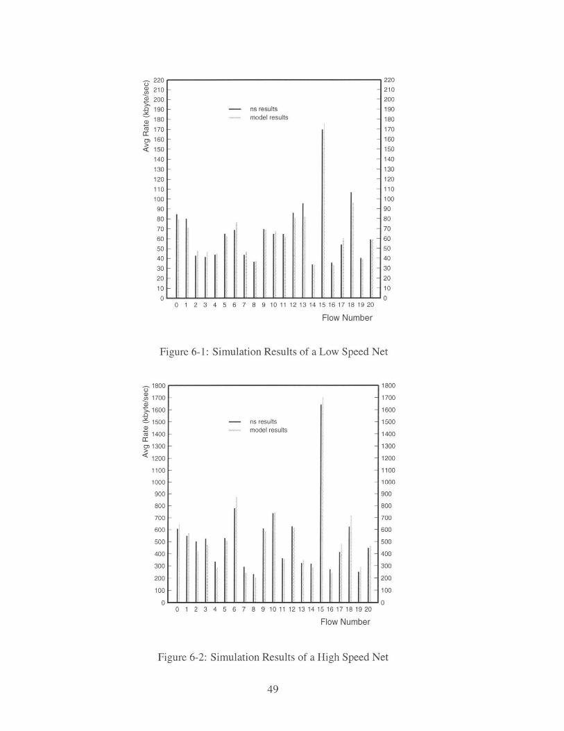
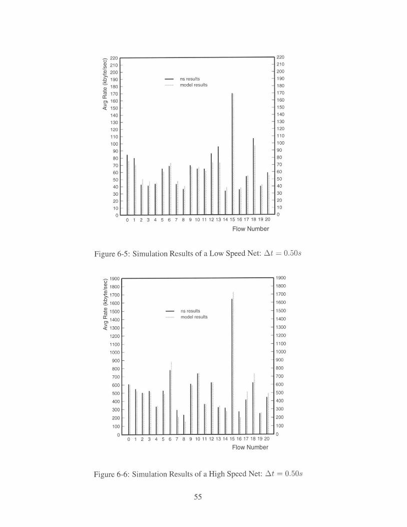
6.3.2 Results

We tested the model's simulation results with those of ns. We designed two test nets. The

first one is the test net introduced in Chap 5. The other one is a high speed net with the

same topology but each link's capacity is increased by a factor of 10. Links connecting the

end user to the subnet are of capacity 80.0Mb. A link connecting intra-localnet routers is

of capacity 16Mb. A link connecting inter-localnet routers is of capacity 24Mb. And a link

connecting inter-domain routers is of capacity 32Mb. We also have 21 flows. The results

are listed in Figure 6-1 and Figure 6-2.

The parameters for RED are minth = 10, maxth = 25, maxp = 0.2. In the simulation

of ns , we use tcp-reno connections to get fast recovery and fast retransmit.

If we assume the results of ns are accurate, the average error of the results for the low

speed net is 6.4%. The one for the high speed net is 9.0%.

We are very interested in the speed of the two methods. In the low speed net test, ns

wins. It takes ns about 65 seconds to do a 100 seconds simulation. For the model, it costs

about 110 seconds. In a low speed net, each flow can only send a small window size of

packets every round trip time. Every state of a packet causes an event. Since the cost of

packet by packet event driven simulation is proportional to the number of events, if the total

number of events is rather small, ns is not slow. However, in the test of a high speed net, it

220

' 210

200

- 190

180

O 170

co 160

< 150

140

130

120

110

100

90

80

70

60

50

40

30

20

100

-1800

co 1700

,1600

1500

ca 1400

c 1300

1200

1100

1000

900

800

700

600

500

400

300

200

100

0

0 1 2 3 4 5 6 7 8 9 10 11 12 13 14 15 1617 18 19 20

Flow Number

Figure 6-1: Simulation Results of a Low Speed Net

0 1 2 3 4 5 6 7 8 9 10 11 12 13 14 15 16 17 18 19 20

1800

1700

1600

1500

1400

1300

1200

1100

1000

900

800

700

600

500

400

300

200

100

0

Flow Number

Figure 6-2: Simulation Results of a High Speed Net

- ns resultsmodel results

- ns resultsmodel results

II I i . . . . . . .. .. . . . .~ _ _ _ _

takes ns about 1.3 hours to do a 100 seconds simulation. For the model, the cost is about

11 seconds. The increase of the cost of ns is due to the increase of each flow's window

size, which results in the increase of events. A packet by packet event driven simulator

has the limit of simulating high speed networks. The decrease of the cost of the model

is due to two reasons. One reason is that in the high speed net with the same number of

flows, the net is lightly loaded. The number of packet drops is reduced. A flow has more

chances to increase its window size by one than it has in a low speed net. Also, it has less

chance to cut its window size by half than it has in a low speed net. In this case, links'

congestion states do not change dramatically. When an event happens, if we assume the set

of congested links is the same as the last event, the assumption is right in most cases. So

we do not need to invoke the original a iteration algorithm. The other reason is if a flow

with a large window cuts its window size by half, it will greatly reduce the congestion of

the network. The network may change from a slightly congested to a non-congested state.

For a non-congested or a net with a few congested links, the cost of solving the equations

is reduced. As the model's cost is mainly increased with the number of flows, unlike ns,

the increase of window sizes does not increase its cost. Therefore, the test of a high speed

net is much faster than the low one.

6.4 The Time Driven Simulation

6.4.1 The Simulating Method

In this section, we study a new simulating method. The model is designed to calculate

the steady state parameters of a network. It is possible that just after one flow changes

its window size, the queue lengths do not change immediately. It may take a short period

for the network to reach a new steady state. Based on this idea, we implemented the time

driven simulation.

We take a 'snapshot' of the simulated network every delta time. Based on the parame-

ters caught at this time, we decide how each flow will change its window size. We assume

each flow will keep its window size within the next delta time. When the next delta time

passes, we take the snapshot again and decide what will happen in the delta time after this

one. Thus the simulation proceeds.

How to choose a proper delta time is a common difficult problem to all time driven

simulations. In window based flow control networks, flows change their window sizes

according to their own round trip times. It is unlikely that there is a global synchronization

that flows change their window sizes if the dropping mechanism is RED. Our simulation

is an approximation. Thus the delta time we choose should base on flows' round trip time.

The simulating result is sensitive to the value of the delta time. Usually, the delta time

should not be less than the largest round trip time among all flows.

Another issue is how to simulate the dropping mechanism of RED. As mentioned

above, we choose the same time interval for each flow to change their window sizes. If

the time interval is larger than a flow's round trip time, in our simulation, we favor this flow

by reducing its packet drop probability since its window size can be cut down at most at

the frequency of every interval time, while its window size can still be increased by one

every round trip time; on the other hand, if the time interval is shorter than a flow's round

trip time, we increase the packet drop probability of this flow since we can cut down its

window size every delta time. As flows have different round trip times, no matter how

we choose the time interval, such problems exist. Thus, a short round trip flow is likely

to have a larger rate share than it should have and vice versa. To compensate for that,

we drop a flow's packet according to its rate share of a congested link's capacity and we

only let the packets in the current queue pass RED filters. Since the number of a flow's

backlogged packets at a congested link is proportional to its share of the capacity1 , if we

drop every single packet according to the rate share of the flow which the packet belongs

to, the net probability of a flow getting a packet drop at each delta time is proportional to

the square of its rate share. This is different from RED. In RED, when the queue length is

between the minimum and the maximum thresholds, every single packet from any flow has

the same dropping probability. So the probability of a flow getting a packet drop is roughly

linear to its rate. We also tested several other dropping mechanism. Here we only list the

1If the link is congested, it is transmitting packets all the time. In the steady state, the more backloggedpackets a flow has at this link, a more rate share it could achieve.

implementation and results about the above dropping method.

The following pseudo-code is for deciding flows' window sizes within the next delta

time.

at time t

if t > the total simulating time, stop

for each flow j

mark = 0

for each link i flow j across

if link i is not congested

continue

if Ni is between [minth, maxth]

Pa = maxp x "

for each flow j's packet in the current queue of link i

if this packet is going to be dropped according to Pa

mark = 1

break

else if Ni > maxth

mark = 1

if mark == 1

break

if mark == 1

cut flow j's window size by half. If the new window size

is less than one, set it to one.

else

increase flow j's window size by Atrttj

t = t + At

6.4.2 Results

Figure 6-3 are test results when At = 0.30s for a low speed net. We chose such a time

interval because the static round trip time of the test net is ranged from 0.080s to 0.26s. The

220 220

Co 210 210

200 200

190 - ns results - 190

S180 - model results - 180

170 - - 170

0 160 - -160

< 150 - - 150

140 - - 140

130 - - 130

120 - - 120

110t

- 110

100- - 100

90 - - 90

80 - 80

70 - 70

60 I- - 60

50 - 50

40 Ii 4030 30

20 20

10 10

0 00 1 2 3 4 5 6 7 8 9 10 11 12 13 14 15 16 17 18 19 20

Flow Number

Figure 6-3: Simulation Results of a Low Speed Net: At = 0.30s

net is heavily loaded. The real maximum round trip time is around 0.30s. The simulated

time is also 100 seconds. The average running time is 18 seconds. The average error is

8.83%. Figure 6-4 shows the results for simulating a high speed net. At = 0.25s. Since

the capacities of links are increased by 10 times, the maximum static round trip delay is

reduced to 0.24s. The queuing delay is also reduced. So, we chose a smaller At. The

average running time for a 100 seconds simulation is 1.6 seconds. The average error is

6.61%.

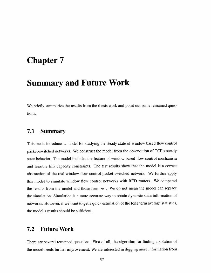
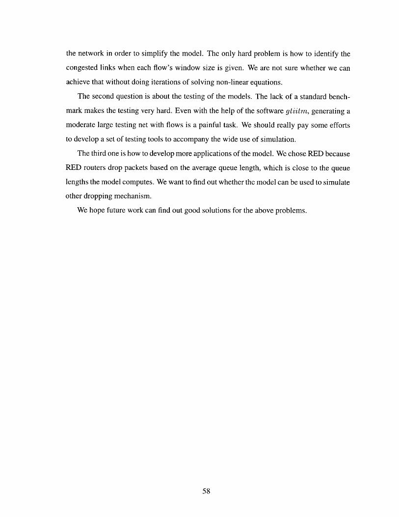
Figure 6-5 and 6-6 are test results when At = 0.50s. For the low speed net, the running

time is nearly 9 seconds. The average error is 8.93%. For the high speed net, the running

time is nearly 0.9 second. The average error is 9.84%. We can see when the time interval At

is increased, the running time is decreased correspondingly. In our simulation mechanism,

we miss more packets drops if At is increased. We favor the short round trip delay flows.

They increase their window sizes faster than they should. Thus long round trip delay flows

get less transmitting rates than they should. The effect can be seen obviously from Figure 6-

- 1900 1900

1800 - - 1800

a 1700 - - 1700

1600 - - 1600

C 1500 - - ns results - 15001400 ........... model results1400 1400

< 1300 - 1300

1200 1200

1100 1100

1000 1000

900 900

800 800

700 700

600 600

500 500

400 - 400

300 300

200 200

100 100

0 00 1 2 3 4 5 6 7 8 9 10 11 12 13 14 15 16 17 18 1920

Flow Number

Figure 6-4: Simulation Results of a High Speed Net: At = 0.25s

4 and 6-6. Flows have high rates in Figure 6-4 are usually short round trip delay flows. They

have higher rates in Figure 6-6. On the contrary, flows have low rates in Figure 6-4 have

lower rates in Figure 6-6.

220

U) 210

200

- 190

180

u 170

a 160

< 150

140

130

120

110

100

90

80

70

60

50

40

30

20

10

0 0 1 3 4 5 6 7 8 9 10 11 12 13 14 15 16 17 18 19 20

0 1 2 3 4 5 6 7 8 9 10 11 12 13 14 15 16 17 18 19 20

Flow Number

Figure 6-5: Simulation Results of a Low Speed Net: At = 0.50s

- 1900

cn 1800" 1700

1600

1500

1400

< 1300

1200

1100

1000

900

800

700

600

500

400

300

200

100

0

- - ns resultsmodel results

-

0 1 2 3 4 5 6 7 8 9 10 11 12 13 14 15 16 17 18 19 20

1900

1800

1700

1600

1500

1400

1300

1200

1100

1000

900

800

700

600

500

400

300

200

100

0

Flow Number

Figure 6-6: Simulation Results of a High Speed Net: At = 0.50s

ns resultsmodel results

56

Chapter 7

Summary and Future Work

We briefly summarize the results from the thesis work and point out some remained ques-

tions.

7.1 Summary

This thesis introduces a model for studying the steady state of window based flow control

packet-switched networks. We construct the model from the observation of TCP's steady

state behavior. The model includes the feature of window based flow control mechanism

and feasible link capacity constraints. The test results show that the model is a correct

abstraction of the real window flow control packet-switched network. We further apply

this model to simulate window flow control networks with RED routers. We compared

the results from the model and those from ns . We do not mean the model can replace

the simulation. Simulation is a more accurate way to obtain dynamic state information of

networks. However, if we want to get a quick estimation of the long term average statistics,

the model's results should be sufficient.

7.2 Future Work

There are several remained questions. First of all, the algorithm for finding a solution of

the model needs further improvement. We are interested in digging more information from

the network in order to simplify the model. The only hard problem is how to identify the

congested links when each flow's window size is given. We are not sure whether we can

achieve that without doing iterations of solving non-linear equations.

The second question is about the testing of the models. The lack of a standard bench-

mark makes the testing very hard. Even with the help of the software gtiitm, generating a

moderate large testing net with flows is a painful task. We should really pay some efforts

to develop a set of testing tools to accompany the wide use of simulation.

The third one is how to develop more applications of the model. We chose RED because

RED routers drop packets based on the average queue length, which is close to the queue

lengths the model computes. We want to find out whether the model can be used to simulate

other dropping mechanism.

We hope future work can find out good solutions for the above problems.

Bibliography

[1] Dimitri Bertsekas and Robert Gallager. Data Networks. Prentice-Hall, Inc, 1992.

[2] http://netweb.usc.edu/vint/. VINT: Virtual InterNetwork Testbed.

[3] http://www nrg.ee.lbl.gov/ns/. ns version 1 - LBNL Network Simulator.

[4] V. Jacobson. Congestion Avoidance and Control. In Proceedings of the ACM SIG-

COMM'88, August 1988.

[5] William H. Press, Saul A. Teukolsky, William T. Vetterling, and Brian P. Flannery.

Numerical Recipes in C. the Press Syndicate of the University of Cambridge, 1992.

[6] Floyd S. and Jacobson V. Random Early Detection gateways for Congestion Avoid-

ance. IEEE/ACM Transactions on Networking, 1(4), August 1993.

[7] Anlu Yan and Wei-Bo Gong. Fluid Simulation for High Speed Networks. In Proceed-

ings of the 15th International Teletraffic Congress, June 1997.