A mid-air collision warning system: Vision-based estimation ofcollision threats for aircraft

Dasun Gunasinghe, Reuben Strydom, Mandyam V. SrinivasanThe University of Queensland, Australia

d.gunasinghe@uq.edu.au

Abstract

This paper describes a vision-based techniquefor predicting whether non-cooperative movingobjects are possible collision threats. The tech-nique predicts the time to minimum separation(TMS), as well as the absolute minimum sep-aration (AMS), to identify object(s) that posea threat based on a predefined safe separationzone. Theory demonstrates how the TMS canbe estimated by measuring changes in the tar-get’s angular visual position as captured by theon-board vision sensor. Furthermore, we showhow the AMS can be estimated from the calcu-lated TMS and the size of the object’s image.The performance of the technique is demon-strated through simulations, as well as in out-door field tests using a rotorcraft.

1 Introduction

Collision avoidance is a key factor in enabling the in-tegration of Unmanned Aircraft (UA) into commercialairspace – be it in civilian or military applications [Phamet al., 2015]. When implementing collision avoidance,one must first establish an early warning system thatdetermines potential conflicts in airspace – for exam-ple, Aircraft Warning System(s) (AWS). Given such asystem, which could ideally rank surrounding obstacles(e.g. aircraft, people, trees, structures, etc.) based oncollision threat, a template for avoidance theory can beestablished.

A review of mid-air collisions between 1961 and 2003[ATSB, 2004] outlines that the probability of a near missbetween aircraft substantially increases in high-densityairspace. Therefore, strict rules and regulations havebeen introduced, and are being continuously updated,to minimise the risk of mid-air collisions [Mcfadyen andMejias, 2016]. Given the larger scale application of AWSin manned airspace, such as the Traffic Alert and Colli-sion Avoidance System (TCAS) and an Automatic De-pendent Surveillance-Broadcast (ADS-B) [Griffith et al.,

2008; Stark et al., 2013; Mcfadyen and Mejias, 2016], wecan see the benefits of adapting such systems to handlethe smaller, cluttered environments that are most likelyto be occupied by small Unmanned Aircraft Systems(UAS). [Hobbs, 1991] states that without such systems,the risk of mid-air collisions would increase by factors of34 and 80 for en-route and terminal areas, respectively.A system with the capability to predict and prevent col-lisions or near misses between aircraft is an importantstep towards ensuring equivalency with current aviationsystems, enabling integration of UA into airspace.

UAS have demonstrated their strengths for applica-tions such as scientific data gathering, surveillance, for-est fire monitoring and military reconnaissance [Lee etal., 2004; Stark et al., 2013]. Many of these applica-tions require low altitude flight, which introduces addi-tional hazards such as pedestrians, trees, power lines etc.Therefore, traditional flight paths and collision warningsystems are unreliable, and often unavailable.

While current regulations are well defined for light andcommercial aircraft, working with small UAS will requirefurther certification. Currently, there is limited trust inthe operation of UAS, where remotely piloted aircraftrules, such as visual line of sight in flight, are imposedfor safety reasons until we reach a level of true autonomyand trust in UAS. Consequently, the future of drone au-tomation in civil airspace will be heavily dependent onthe availability of aircraft warning and avoidance sys-tems, and these systems must comply with the safetystandards of current piloted aircraft.

Current safety standards for large commercial aircraftgenerally involve cooperative AWS (where all aircrafthave knowledge about other aircraft in the vicinity –based on satellite Global Positioning Systems (GPS) andtransponder communication). Some of the major co-operative methods currently used in manned airspaceare TCAS and Traffic Advisory System (TAS), whichrely on transponder communication between aircraft,and ADS-B (satellite-based GPS for aircraft location)[Hobbs, 1991; Griffith et al., 2008; Hottman et al., 2009].

Cooperative systems have demonstrated their safety andreliability through stringent regulations, and years of re-search and testing. However, they require all partici-pating aircraft to have the same technology on-board.This is a significant disadvantage that prevents use onsmaller, light-weight aircraft where size, weight, powerand cost are key factors [Hottman et al., 2009]. Otherdisadvantages include inability to detect ground-basedobstacles such as terrain and urban structures. Thus, inthe context of UAS or light aircraft operating in residen-tial or commercial airspace, it is desirable to implementreliable non-cooperative collision avoidance strategies –where aircraft act individually based on their own sens-ing mechanisms, without relying on information passedbetween nearby aircraft from any central infrastructure.

Non-cooperative systems have the advantage that theydo not require communication between the conflictingaircraft. Furthermore, they have the capacity to detectnot only airborne threats, but also ground-based vehi-cles and structures. These non-cooperative systems canbe classified into (i) active systems that use radar, laser,and sonar systems to detect obstacles [Lee et al., 2004;Griffith et al., 2008; Hottman et al., 2009], and (ii) sys-tems that employ passive sensing, using Electro-Optical(EO) or Infra-red (IR) technology [Griffith et al., 2008;Hottman et al., 2009; Harmsen and Liu, 2016]. EO andIR sensors have the advantage of low power and weight[Griffith et al., 2008; Harmsen and Liu, 2016].

When considering AWS, the ability to judge the timeto collision/contact (TTC) with sufficient Time For Eva-sion (TFE) is a desirable trait [Lee, 1980], especially inautonomous systems that navigate in cluttered environ-ments. TTC has been used to assess conflict scenariosin many vision-based approaches. The time to contactan object that is on a direct collision course can be es-timated by computing the ratio of the angular size ofthe objects’ image to the rate of expansion of the image(e.g. [Lee, 1980; Lee et al., 2004]). This calculation ofTTC does not require information about the absolutesize of the object, or the velocities of the aircraft andthe object.

The key variables being measured for this computationare the angular size of the object’s image, and the rateof its expansion. While these variables can be used topredict the TTC accurately when the angular size of theobject’s image is large, they become imprecise and im-practical when the image is initially small for a long time,and then begins to expand rapidly when sufficiently closeto the time at which collision occurs. This is dangerous,as looming cues allow little TFE. Furthermore, it doesnot provide information on whether the encounter willactually result in a collision or a near miss, and if it isa near miss, what the minimum separation will be. Themethod we propose here addresses these problems, and

provides an estimate of the Time to Minimum Separa-tion (TMS), as well as the Absolute Minimum Separa-tion (AMS). The technique also allows us to rank threatlevels during flight in the vicinity of several UAS, basedon calculations of the TMS and the AMS for each of theaircraft in the vicinity.

The performance of our system is validated throughsimulations (both in MATLAB and our realistic vir-tual environment), as well as through field tests usinga ground and an airborne vehicle (in this case, a rotor-craft). We use a vision system as the primary sensor,due to its low cost, weight, and multi-functionality (e.g.egomotion computation and target detection).

The paper presents the problem definition in section2. The theory, and the implementations in simulationsand field tests are then discussed in sections 3, 4, 5 and6. Finally, sections 7, 8, 9 and 10 discuss the limita-tions, applications and advantages, and future scope ofthe method.

2 Problem Definition

We develop a method, which uses a vision-based geo-metrical approach, to compute the Time to MinimumSeparation (TMS) and the Absolute Minimum Separa-tion (AMS). TMS and AMS provide valuable informa-tion that can be used to predict scenarios including nearmisses, i.e. for trajectories that produce a near missbut not a collision, as well as safe, distant fly-bys. Fur-thermore, this approach enables a UAS to theoreticallyestimate in advance the AMS between itself and all ofthe aircraft operating in its vicinity. Using this infor-mation, we can determine collision avoidance strategiesby ranking levels of threat. One strategy to obtain aquantitative threat measure would be to rank the vari-ous aircraft – first by TMS, and then by AMS – once theAMS has been estimated reliably. The focus of this pa-per is the theoretical derivation of TMS and AMS, andthe testing of the feasibility of this approach for earlywarning of near-misses.

Our analysis makes the following assumptions:

1. The velocity of the UAS and the conflicting targetsare constant. This is reasonable given that, at leastfor relatively small time scales, most aircraft willmaintain a constant heading and velocity when fly-ing along pre-defined trajectories.

2. It is assumed that the target has been detected, andthat its bearing can be computed – only the bear-ing to the target is required for our algorithm tocompute TMS.

3. The instantaneous absolute range to the target canbe directly sensed, or inferred.

3 Theory

The following sections describe the derivation of the the-ory for TMS, as well as the calculation of AMS usinginstantaneous range information.

3.1 Time to Minimum Separation (TMS)

The theory is based on a geometrical approach, similarto a method conducted by [Han and Bang, 2004] and[Park et al., 2008]. However, both of those approachesassume considerable prior knowledge about the state ofthe conflict (near-miss) UAS, including its position andvelocity. For example, [Park et al., 2008] assume theavailability of a system such as ADS-B. Our approachuses only on-board vision, and does not rely on ADS-B.Additionally, our approach takes into account scenarioswhere (i) both the target and the aircraft are moving;(ii) the target is stationary and the aircraft is moving;and (iii) the aircraft is stationary and the target is mov-ing. We first develop our algorithm for flight in a 2Dplane, and show that TMS can be determined by non-cooperative means. We then extend the algorithm toprovide a full 3D solution.

(!3*,'3*)(!4*, '4*)

((,5,(.5 )

((,6,(.6 )

(!3, '3)

(!4,'4)

θ

Rotorcraft

ConflictingUAS

'

!

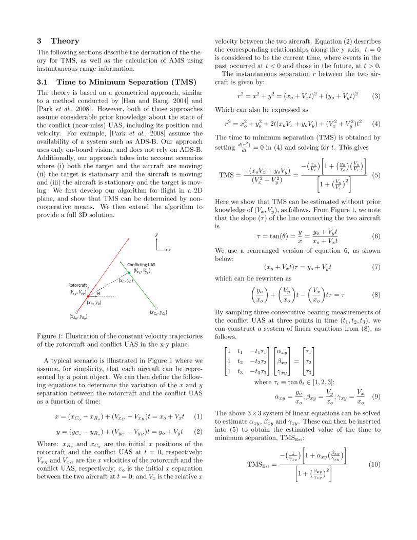
Figure 1: Illustration of the constant velocity trajectoriesof the rotorcraft and conflict UAS in the x-y plane.

A typical scenario is illustrated in Figure 1 where weassume, for simplicity, that each aircraft can be repre-sented by a point object. We can then define the follow-ing equations to determine the variation of the x and yseparation between the rotorcraft and the conflict UASas a function of time:

x = (xCo− xRo

) + (VxC− VxR

)t = xo + Vxt (1)

y = (yCo − yRo) + (VyC − VyR)t = yo + Vyt (2)

Where: xRoand xCo

are the initial x positions of therotorcraft and the conflict UAS at t = 0, respectively;VxR

and VxCare the x velocities of the rotorcraft and the

conflict UAS, respectively; xo is the initial x separationbetween the two aircraft at t = 0; and Vx is the relative x

velocity between the two aircraft. Equation (2) describesthe corresponding relationships along the y axis. t = 0is considered to be the current time, where events in thepast occurred at t < 0 and those in the future, at t > 0.

The instantaneous separation r between the two air-craft is given by:

r2 = x2 + y2 = (xo + Vxt)2 + (yo + Vyt)

2 (3)

Which can also be expressed as

r2 = x2o + y2o + 2t(xoVx + yoVy) + (V 2x + V 2

y )t2 (4)

The time to minimum separation (TMS) is obtained by

setting d(r2)dt = 0 in (4) and solving for t. This gives

TMS =−(xoVx + yoVy)

(V 2x + V 2

y )=

−(xo

Vx

)[1 +

(yoxo

)(Vy

Vx

)][1 +

(Vy

Vx

)2] (5)

Here we show that TMS can be estimated without priorknowledge of (Vx, Vy), as follows. From Figure 1, we notethat the slope (τ) of the line connecting the two aircraftis

τ = tan(θ) =y

x=yo + Vyt

xo + Vxt(6)

We use a rearranged version of equation 6, as shownbelow:

(xo + Vxt)τ = yo + Vyt (7)

which can be rewritten as(yoxo

)+

(Vyxo

)t−(Vxxo

)tτ = τ (8)

By sampling three consecutive bearing measurements ofthe conflict UAS at three points in time (t1, t2, t3), wecan construct a system of linear equations from (8), asfollows.1 t1 −t1τ1

1 t2 −t2τ21 t3 −t3τ3

αxyβxy

γxy

=

τ1τ2τ3

where τi ≡ tan θi ∈ [1, 2, 3];

αxy =yoxo

;βxy =Vyxo

; γxy =Vxxo

(9)

The above 3×3 system of linear equations can be solvedto estimate αxy, βxy and γxy. These can then be insertedinto (5) to obtain the estimated value of the time tominimum separation, TMSEst:

TMSEst =

−(

1γxy

)[1 + αxy

(βxy

γxy

)][1 +

(βxy

γxy

)2] (10)

3.2 Absolute Minimum Separation (AMS)

Assuming that we know the current range to the conflictUAS (and therefore xo and yo, from knowledge of thetarget bearing), we can insert these values into (4) toestimate the absolute minimum separation (AMS), asfollows:

AMS2 = x2o + y2o + 2(TMSEst)

(xoVx + yoVy) + (V 2x + V 2

y )(TMSEst)2 (11)

where:

• xo & yo are the x and y separations between therotorcraft and the conflict UAS (current range);

• Vx = γxy × xo;• Vy = βxy × xo;

3.3 Extension of Theory to 3D

The derivation of TMS for the 3D situation is analogousto the 2D case. We note that:

r2 = (xo + Vxt)2 + (yo + Vyt)

2 + (zo + Vzt)2 (12)

where zo is the initial position difference between theconflict UAS and the rotorcraft in the z dimension, andVz is the relative velocity between the conflict UAS and

the rotorcraft in the z dimension. Setting d(r2)dt = 0, we

derive

TMS3DTheory =

−(xoVx + yoVy + zoVz)

(V 2x + V 2

y + V 2z )

(13)

We estimate TMS3DTheory from (13) by using a procedure

analogous to the 2D case, but now including the x-zplane. It can be shown that:

TMS3DEst =

−(

1γxy

)[1 + αxy

(βxy

γxy

)+ αxz

(βxz

γxz

)][1 +

(βxy

γxy

)2+(βxz

γxz

)2] (14)

where αxz =yoxo

;βxz =Vzxo

; γxz =Vxxo

Proceeding as in the 2D case, we insert TMS3DEst into the

3D range function (12) to derive the estimate of the AMSin 3D:

(AMS3DEst)

2 = x2o + y2o + z2o+

2(TMS3DEst)(xoVx + yoVy + zoVz)+

(V 2x + V 2

y + V 2z )(TMS3D

Est)2 (15)

where:

• zo is the z separation between the rotorcraft and theconflict UAS;

• Vz = βxz × xo;

3.4 Special Cases

If the absolute bearing of the target is constant overtime, the three equations in (9) will be identical, hencethe matrix will be singular. This condition representsone of three possible situations: (i) If the angular sizeof the target is constant, the range of the target is con-stant. This implies that the target is moving in the samedirection and at the same speed, which can be classifiedas non-threatening, requiring no further action. (ii) Ifthe angular size of the target decreases steadily, the tar-get is receding from the UAS – also classified as non-threatening. (iii) If the angular size of the target in-creases steadily, the target is approaching the UAS on adirect collision course. This is obviously a severe threat.The instantaneous distance to the target (and the rate ofdecrease of this distance) can be inferred from the rateof change of the target’s angular size. The TTC canthen be inferred from this information, or even withoutknowledge of the object’s absolute size by using well es-tablished methods for estimating the TTC (e.g. [Lee,1980]). Methods for dealing with these special cases arewell established. Our study focuses instead on near-missscenarios, where it is important to assess the threat levelby estimating the TMS and the AMS.

4 Implementation

This section describes the implementation of our methodfor estimation of TMS and AMS for the virtual envi-ronment and outdoor field tests. To estimate TMS andAMS the following information is required: the aircraft’segomotion, location of the target in the image and thedistance to the target.

Our vision system computes the egomotion of the ro-torcraft using an optic flow and stereo technique, asdetailed in [Strydom et al., 2014; Thurrowgood et al.,2014]. Object detection (and visual bearing computa-tion) is based on a colour detector, utilised for its sim-plicity in the same manner as step (ii) and (iii) in section3 of [Strydom et al., 2015]. We assume that the physicalsize of the object is known, which allows us to computethe instantaneous range to the target from the angularsize of the object in the image – similar to [Molloy et al.,2014]. This computation is important for the estimationof AMS. Alternative methods such as radar can also beused, if available, for range and bearing estimation. Notethat the focus of this research is not target detection perse, but rather to demonstrate the validity of our theoryto compute TMS and AMS.

5 Validation

In this section, we describe the validation of the theoret-ical derivations through simulations, initially in a MAT-LAB environment (important for estimating TMS (14),

and AMS (15) in a real time setting and with simulatednoise) and then in a flight simulator (incorporation of therotorcraft’s dynamics, and visual detection of a conflictUAS (represented by a red ball), including realistic sim-ulations of noise at various levels of the system). Thesetests provide a comprehensive understanding of the pre-diction of these parameters at distances larger than 20m– in comparison to the field tests where the ball is de-tected at approximately 5m.

5.1 MATLAB Implementation

For the system to effectively rank threats from multipleaircraft, an initial simulation in real-time was conductedin MATLAB, as a proof of concept. The simulation useda single-point representation of the rotorcraft and 3 dif-ferent conflict UAS (Figure 2). For each trial, the (con-stant) 3D velocity of the rotorcraft and the conflict UAS’were specified by a random number generator. As thepurpose of this exercise was to validate the basic theory,the aircraft dynamics were omitted.

Figure 2: Illustration of trajectories of a rotorcraft (red)and 3 conflicting UAS (blue): T1, T2 and T3. T2 hasa negative TMS, and therefore poses no threat. T1 ispositive and thus represents a potential threat. However,the threat level (as defined by the minimum acceptableseparation) is negative and does not require action. T3has a positive TMS and exhibits a positive threat level,and therefore requires an evasive manoeuvre.

Calculation and Plotting of TMS and AMS

First, an initial moving window is defined to sample thebearing information of visible targets. In theory, threebearings, sampled at three different times, are requiredfor estimating the TMS (See Theory Section). We set awindow size larger than the minimum 3 bearing window,and solve for the TMS using a pseudo-inverse approach.In this example, a window size of 9 was selected as a 3×9 pseudo-inverse demonstrated reliable results. Figure3(a) compares the theoretical calculation of TMS (14)and AMS (15) with the running real-time TMS and AMS

for the target posing the highest threat – the smallestAMS – (T3) from Figure 2 under no simulated noise.Note the delay in estimation of 9 frames (0.4 sec) due tothe selected window size.

0.4 1.5 2.7 3.8 5.0Time from Initial Estimation (0.4) (sec)

-2

0

2

4

6

8

10Estimation of TMS and AMS for T3 Under No Noise

TMS TheoreticalTMS EstimatedAMS TheoreticalAMS Estimated

-2

0

2

4

6

8

10

AMS(m

)

TMS(sec)

(a)

(b)

0.4 1.5 2.7 3.8 5.0Time from Initial Estimation (0.4) (sec)

-2

0

2

4

6

8

10

TMS(sec)

Estimation of TMS and AMS for T3 Under Noise

TMS TheoreticalTMS EstimatedAMS TheoreticalAMS Estimated

-2

0

2

4

6

8

10

AMS(m

)

Figure 3: Comparison of running estimate of TMS andAMS under (a) no noise and (b) with noise against thetheoretically expected values for T3. The dashed redlines denote the point of minimum separation. Note thatthe AMS value remains constant, as expected. Shadedregion represents a possible reliable detection zone.

It is clear from Figure 3(a) that the technique correctlypredicts the theoretical TMS and AMS – the theoreti-cally expected values of TMS (magenta) and AMS (red)are overlaid perfectly by the estimated TMS (blue) andAMS (green). Following this initial proof of concept,simulated noise is added to the measurements of thebearings and ranges. Figure 3(b) illustrates the resultsobtained for flight trajectory T3 when noise of ±0.05o

and ±0.5m is added to the bearing and range measure-ments, respectively.

Refinement of Technique

While the initial results are promising, they also reveal asensitivity to noise, particularly in situations where theinitial target bearing varies slowly with time. It is evi-dent that the estimated TMS and AMS begin to showgood agreement with the theoretically expected valuesjust a few seconds prior to the instant of minimum sep-aration, as shown by the shaded section in Figure 3(b).The reason for this is that when the target is far away,

its angular bearing slowly changes and is buried in thenoise, leading to noisy and unreliable computations ofthe pseudo-inverse. The time at which the running esti-mates of TMS and AMS first become reliable (as shownby the left boundary of the grey section) defines the in-stant at which a reliable alert can be issued, and an eva-sive response undertaken. We call the temporal widthof the grey box the Time for Evasion (TFE). The TFEspecifies the time that is available for the execution ofan evasive response.

Fortunately, as we shall show below in the flight sim-ulator tests (section 5.2), pre and post filtering meth-ods can be used effectively to reduce some of the com-pounded error in the estimates of TMS and AMS. Toimprove the efficacy of pre and post filtering, (i) Thetemporal separation between the sampled bearings is in-creased from 1 to 6, in order to register larger changesof the target bearing. The 9 bearings required for thepseudo-inverse computation are now sampled at frames[1, 7, 13, 19, 25, 31, 37, 43, 49], resulting in a windowsize of 49. (ii) A second order polynomial fit is performedon the 9 target bearings measured over this window, toobtain more reliable bearing estimates. (iii) A running49-point median filter is used to post-filter the pseudo-inverse results to obtain the TMS and AMS estimates.While these operations reduce the noise, they also intro-duce a delay in the calculation of TMS and AMS. Theselected window size of 49 is the smallest optimal windowgiven a test from 9 through to 99 frames. It was evidentthat a larger TFE was determinable at 49 frames andabove, thus this window size was selected to induce thesmallest delay (1.96 sec before the first pseudo-inverse re-sult becomes available). Furthermore, the post-filteringintroduces another 1.96 second delay before the first me-dian values of TMS and AMS are generated. Thus, thereis a 3.92 sec delay between the acquisition of the firsttarget bearing sample, and the generation of the firstfiltered values of TMS and AMS.

Evaluation of Potential Threats

To determine the potential threat from a UAS, we firstexamine whether the computed TMS is positive or neg-ative. If the TMS is negative, this implies that the mini-mum separation would have already occurred in the past,so that this UAS is no longer a threat (e.g. trajectoryT2 in Figure 2). It is only the aircraft that generatepositive TMS values that imply potential future threats;these are the only aircraft that need to be consideredfurther. We can rank the threat level of these aircraftby computing a threat level parameter:

Threat Level = (Safety range - AMS)

The safety range is the minimum allowable separationbetween the two aircraft, for a safe fly-by. Thus, a threat

exists if TMS > 0, and the threat level is positive; themore positive the threat level, the greater the threat (e.g.trajectory T3 in Figure 2). A positive threat level closeto (safety range) implies a near-direct collision, becausethe AMS is then very close to zero.

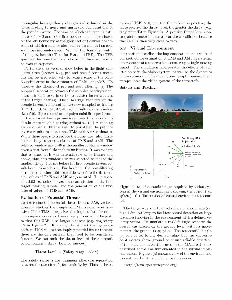
5.2 Virtual Environment

This section describes the implementation and results ofour method for estimation of TMS and AMS in a virtualenvironment of a rotorcraft encountering a single movingtarget. The simulation incorporates the effects of real-istic noise in the vision system, as well as the dynamicsof the rotorcraft. The Open Scene Graph 1 environmentencapsulates the vision system of the rotorcraft.

Set-up and Testing

(a)

(b)

!"#$%&'()*+&'&,-."(/*,0**"(1'&2*3,.'-*4(5(!!"#$

6."7%-3,-"#(8!)(1'&2*3,.'-*4

9*%.3-,:(5(;<=(>?4

%

& =@(>

=@(>

A.,.'3'&7,9*%.3-,:(5(;>?4

1;

1=

1B

1C

1D

1E 1F=G<=G(>

Figure 4: (a) Panoramic image acquired by vision sys-tem in the virtual environment, showing the object (redsphere). (b) Illustration of virtual environment scenar-ios.

The target was a virtual red sphere of known size (ra-dius 1.5m set large to facilitate visual detection at largedistances) moving in the environment with a defined ve-locity vector. To simulate a real-life flight scenario theobject was placed on the ground level, with its move-ment in the ground (x-y) plane. The rotorcraft’s height(z) can be set to any desired value, but was chosen tobe 3 metres above ground to ensure reliable detectionof the ball. The algorithm used in the MATLAB studydescribed above was implemented in the virtual imple-mentation. Figure 4(a) shows a view of the environment,as captured by the simulated vision system.

1http://www.openscenegraph.org/

0246810121416Time to Minimum Separation (sec)

0

2

4

6

8

10

12MeanRMSerrorin

TMS(sec)

Mean RMS Curves for the Seven Trajectories (TMS)

Trajectory 1Trajectory 2Trajectory 3Trajectory 4Trajectory 5Trajectory 6Trajectory 7

(a)

0246810121416Time to Minimum Separation (sec)

0

0.5

1

1.5

2

2.5

MeanRMSerrorin

relative

AMS

Mean RMS Curves for the Seven Trajectories (AMS)

Trajectory 1Trajectory 2Trajectory 3Trajectory 4Trajectory 5Trajectory 6Trajectory 7

(b)

0246810121416Time to Minimum Separation (sec)

00.10.20.30.40.50.60.70.80.9

1

Delta

Theta(x-y)per

Frame(deg) Mean Delta Theta for the Seven Trajectories

Trajectory 1Trajectory 2Trajectory 3Trajectory 4Trajectory 5Trajectory 6Trajectory 7

(c)

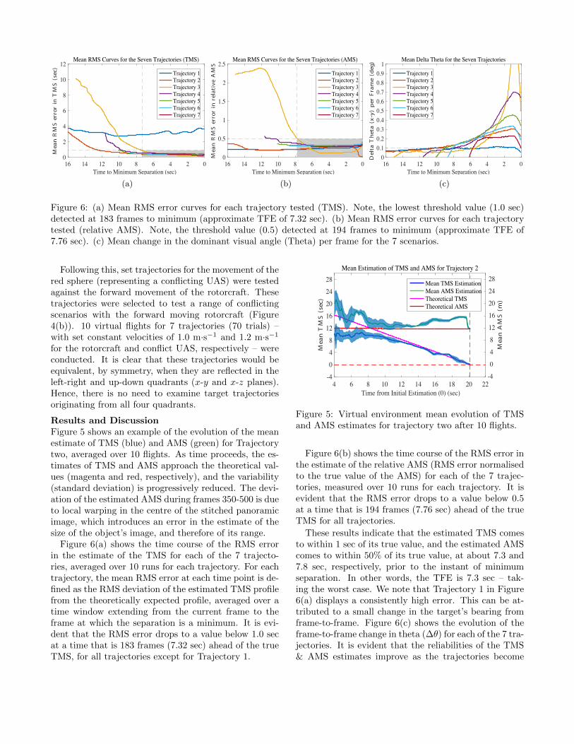
Figure 6: (a) Mean RMS error curves for each trajectory tested (TMS). Note, the lowest threshold value (1.0 sec)detected at 183 frames to minimum (approximate TFE of 7.32 sec). (b) Mean RMS error curves for each trajectorytested (relative AMS). Note, the threshold value (0.5) detected at 194 frames to minimum (approximate TFE of7.76 sec). (c) Mean change in the dominant visual angle (Theta) per frame for the 7 scenarios.

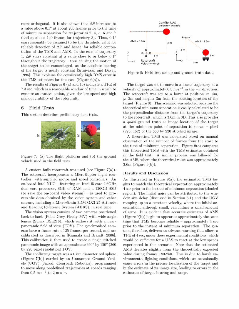
Following this, set trajectories for the movement of thered sphere (representing a conflicting UAS) were testedagainst the forward movement of the rotorcraft. Thesetrajectories were selected to test a range of conflictingscenarios with the forward moving rotorcraft (Figure4(b)). 10 virtual flights for 7 trajectories (70 trials) –with set constant velocities of 1.0 m·s−1 and 1.2 m·s−1

for the rotorcraft and conflict UAS, respectively – wereconducted. It is clear that these trajectories would beequivalent, by symmetry, when they are reflected in theleft-right and up-down quadrants (x-y and x-z planes).Hence, there is no need to examine target trajectoriesoriginating from all four quadrants.

Results and DiscussionFigure 5 shows an example of the evolution of the meanestimate of TMS (blue) and AMS (green) for Trajectorytwo, averaged over 10 flights. As time proceeds, the es-timates of TMS and AMS approach the theoretical val-ues (magenta and red, respectively), and the variability(standard deviation) is progressively reduced. The devi-ation of the estimated AMS during frames 350-500 is dueto local warping in the centre of the stitched panoramicimage, which introduces an error in the estimate of thesize of the object’s image, and therefore of its range.

Figure 6(a) shows the time course of the RMS errorin the estimate of the TMS for each of the 7 trajecto-ries, averaged over 10 runs for each trajectory. For eachtrajectory, the mean RMS error at each time point is de-fined as the RMS deviation of the estimated TMS profilefrom the theoretically expected profile, averaged over atime window extending from the current frame to theframe at which the separation is a minimum. It is evi-dent that the RMS error drops to a value below 1.0 secat a time that is 183 frames (7.32 sec) ahead of the trueTMS, for all trajectories except for Trajectory 1.

4 6 8 10 12 14 16 18 20 22Time from Initial Estimation (0) (sec)

-4

0

4

8

12

16

20

24

28

MeanTMS(sec)

Mean Estimation of TMS and AMS for Trajectory 2

Mean TMS EstimationMean AMS EstimationTheoretical TMSTheoretical AMS

-4

0

4

8

12

16

20

24

28

MeanAMS(m

)

Figure 5: Virtual environment mean evolution of TMSand AMS estimates for trajectory two after 10 flights.

Figure 6(b) shows the time course of the RMS error inthe estimate of the relative AMS (RMS error normalisedto the true value of the AMS) for each of the 7 trajec-tories, measured over 10 runs for each trajectory. It isevident that the RMS error drops to a value below 0.5at a time that is 194 frames (7.76 sec) ahead of the trueTMS for all trajectories.

These results indicate that the estimated TMS comesto within 1 sec of its true value, and the estimated AMScomes to within 50% of its true value, at about 7.3 and7.8 sec, respectively, prior to the instant of minimumseparation. In other words, the TFE is 7.3 sec – tak-ing the worst case. We note that Trajectory 1 in Figure6(a) displays a consistently high error. This can be at-tributed to a small change in the target’s bearing fromframe-to-frame. Figure 6(c) shows the evolution of theframe-to-frame change in theta (∆θ) for each of the 7 tra-jectories. It is evident that the reliabilities of the TMS& AMS estimates improve as the trajectories become

more orthogonal. It is also shown that ∆θ increases toa value above 0.1o at about 200 frames prior to the timeof minimum separation for trajectories 2, 4, 5, 6 and 7(and at about 140 frames for trajectory 3). Thus, 0.1o

can reasonably be assumed to be the threshold value forreliable detection of ∆θ, and hence, for reliable compu-tation of the TMS and AMS. In the case of trajectory1, ∆θ stays constant at a value close to or below 0.1o

throughout the trajectory – thus causing the motion ofthe target to be camouflaged, as the absolute bearingof the target is nearly constant [Srinivasan and Davey,1995]. This explains the consistently high RMS error inthe TMS estimates for this case (Figure 6(a)).

The results of Figures 6 (a) and (b) indicate a TFE of7.3 sec, which is a reasonable window of time in which toexecute an evasive action, given the low speed and highmanoeuvrability of the rotorcraft.

6 Field Tests

This section describes preliminary field tests.

(a) (b)

Figure 7: (a) The flight platform and (b) the groundvehicle used in the field tests.

A custom built rotorcraft was used (see Figure 7(a)).The rotorcraft incorporates a MicroKopter flight con-troller, with supplied motor and speed controllers. Anon-board Intel NUC – featuring an Intel i5 core 2.6GHzdual core processor, 8GB of RAM and a 120GB SSD(to save the on-board video stream) – is used to pro-cess the data obtained by the vision system and othersensors, including a MicroStrain 3DM-GX3-25 Attitudeand Heading Reference System (AHRS), in real time.

The vision system consists of two cameras positionedback-to-back (Point Grey Firefly MV) with wide-anglelenses (Sunex DSL216), which endows it with a near-panoramic field of view (FOV). The synchronised cam-eras have a frame rate of 25 frames per second, and arecalibrated as described in [Kannala and Brandt, 2006].This calibration is then used to create a single stitchedpanoramic image with an approximate 360o by 150o (360by 220 pixel resolution) FOV.

The conflicting target was a 0.8m diameter red sphere(Figure 7(b)) carried by an Unmanned Ground Vehi-cle (UGV) (Jackal, Clearpath Robotics), programmedto move along predefined trajectories at speeds rangingfrom 0.5 m·s−1 to 2 m·s−1.

!

"! "

! "

#$"

%&'$($!)*"

+,-,./.01-234,/5-6$($7"89

"

#: "

! "

;,<145/-$=%'234,/5-6$($7)> "89

%&'$($!)*"

Figure 8: Field test set-up and ground truth data.

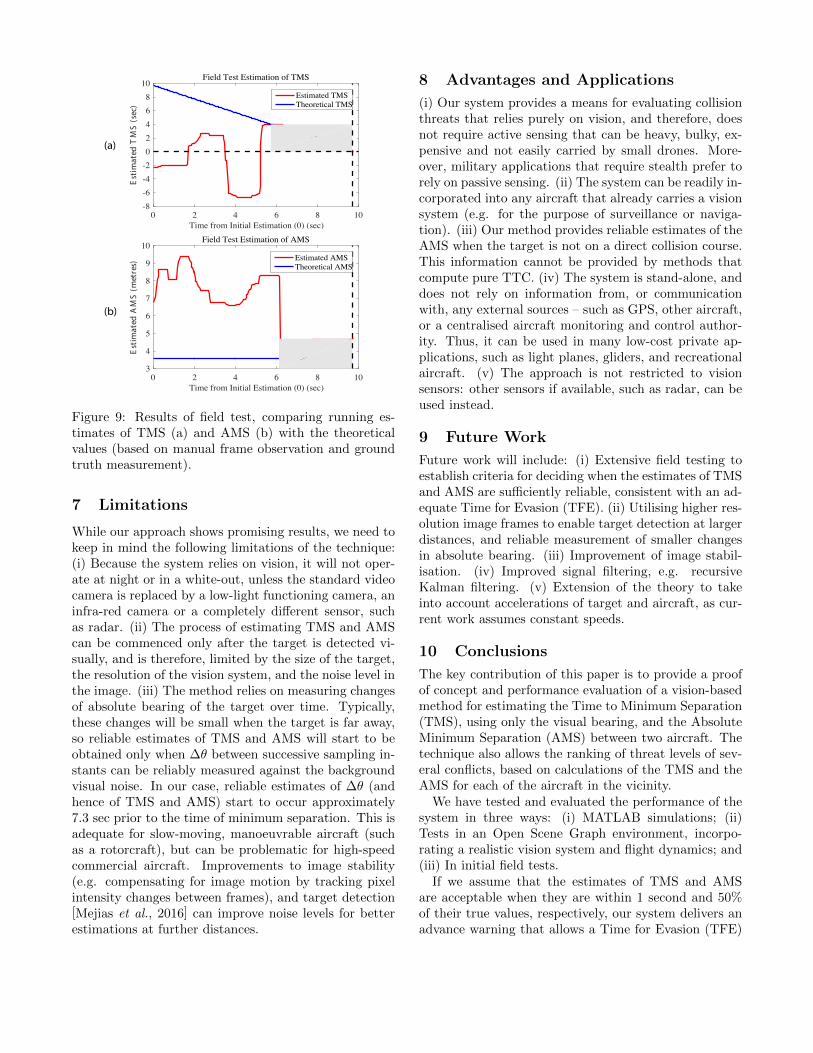
The target was set to move in a linear trajectory at avelocity of approximately 0.5 m·s−1 in the −x direction.The rotorcraft was set to a hover at position x: 4m,y: 3m and height: 3m from the starting location of thetarget (Figure 8). This scenario was selected because thetheoretical minimum separation is easily calculated to bethe perpendicular distance from the target’s trajectoryto the rotorcraft, which is 3.6m in 3D. This also providesa quasi ground truth as image location of the targetat the minimum point of separation is known – pixel(275, 152) of the 360 by 220 stitched image.

A theoretical TMS was calculated based on manualobservation of the number of frames from the start tothe time of minimum separation. Figure 9(a) comparesthis theoretical TMS with the TMS estimates obtainedin the field test. A similar process was followed forthe AMS, where the theoretical value was approximately3.6m (Figure 9(b)).

Results and Discussion

As illustrated in Figure 9(a), the estimated TMS be-gins to match the theoretical expectation approximately4 sec prior to the instant of minimum separation (shadedregion). The initial noise can be attributed to the win-dow size delay (discussed in Section 5.1) and the UGVramping up to a constant velocity, where the initial ac-celeration, although small, can induce a small amountof error. It is evident that accurate estimates of AMS(Figure 9(b)) begin to appear at approximately the sametime that TMS becomes reliable – approximately 4 secprior to the instant of minimum separation. The sys-tem, therefore, delivers an advance warning that allows aTFE of 4 sec, under these experimental conditions, whichwould be sufficient for a UAS to react at the low speedsexperienced in this scenario. Note that the estimatedAMS deviates slightly from the theoretically expectedvalue during frames 180-250. This is due to harsh en-vironmental lighting conditions, which can occasionallycause errors in the precise localisation of the target andin the estimate of its image size, leading to errors in theestimates of target bearing and range.

(a)

(b)

0 2 4 6 8 10Time from Initial Estimation (0) (sec)

-8-6-4-202468

10

Estim

ated

TMS(sec)

Field Test Estimation of TMS

Estimated TMSTheoretical TMS

0 2 4 6 8 10Time from Initial Estimation (0) (sec)

3

4

5

6

7

8

9

10

Estim

ated

AMS(m

etres)

Field Test Estimation of AMS

Estimated AMSTheoretical AMS

Figure 9: Results of field test, comparing running es-timates of TMS (a) and AMS (b) with the theoreticalvalues (based on manual frame observation and groundtruth measurement).

7 Limitations

While our approach shows promising results, we need tokeep in mind the following limitations of the technique:(i) Because the system relies on vision, it will not oper-ate at night or in a white-out, unless the standard videocamera is replaced by a low-light functioning camera, aninfra-red camera or a completely different sensor, suchas radar. (ii) The process of estimating TMS and AMScan be commenced only after the target is detected vi-sually, and is therefore, limited by the size of the target,the resolution of the vision system, and the noise level inthe image. (iii) The method relies on measuring changesof absolute bearing of the target over time. Typically,these changes will be small when the target is far away,so reliable estimates of TMS and AMS will start to beobtained only when ∆θ between successive sampling in-stants can be reliably measured against the backgroundvisual noise. In our case, reliable estimates of ∆θ (andhence of TMS and AMS) start to occur approximately7.3 sec prior to the time of minimum separation. This isadequate for slow-moving, manoeuvrable aircraft (suchas a rotorcraft), but can be problematic for high-speedcommercial aircraft. Improvements to image stability(e.g. compensating for image motion by tracking pixelintensity changes between frames), and target detection[Mejias et al., 2016] can improve noise levels for betterestimations at further distances.

8 Advantages and Applications

(i) Our system provides a means for evaluating collisionthreats that relies purely on vision, and therefore, doesnot require active sensing that can be heavy, bulky, ex-pensive and not easily carried by small drones. More-over, military applications that require stealth prefer torely on passive sensing. (ii) The system can be readily in-corporated into any aircraft that already carries a visionsystem (e.g. for the purpose of surveillance or naviga-tion). (iii) Our method provides reliable estimates of theAMS when the target is not on a direct collision course.This information cannot be provided by methods thatcompute pure TTC. (iv) The system is stand-alone, anddoes not rely on information from, or communicationwith, any external sources – such as GPS, other aircraft,or a centralised aircraft monitoring and control author-ity. Thus, it can be used in many low-cost private ap-plications, such as light planes, gliders, and recreationalaircraft. (v) The approach is not restricted to visionsensors: other sensors if available, such as radar, can beused instead.

9 Future Work

Future work will include: (i) Extensive field testing toestablish criteria for deciding when the estimates of TMSand AMS are sufficiently reliable, consistent with an ad-equate Time for Evasion (TFE). (ii) Utilising higher res-olution image frames to enable target detection at largerdistances, and reliable measurement of smaller changesin absolute bearing. (iii) Improvement of image stabil-isation. (iv) Improved signal filtering, e.g. recursiveKalman filtering. (v) Extension of the theory to takeinto account accelerations of target and aircraft, as cur-rent work assumes constant speeds.

10 Conclusions

The key contribution of this paper is to provide a proofof concept and performance evaluation of a vision-basedmethod for estimating the Time to Minimum Separation(TMS), using only the visual bearing, and the AbsoluteMinimum Separation (AMS) between two aircraft. Thetechnique also allows the ranking of threat levels of sev-eral conflicts, based on calculations of the TMS and theAMS for each of the aircraft in the vicinity.

We have tested and evaluated the performance of thesystem in three ways: (i) MATLAB simulations; (ii)Tests in an Open Scene Graph environment, incorpo-rating a realistic vision system and flight dynamics; and(iii) In initial field tests.

If we assume that the estimates of TMS and AMSare acceptable when they are within 1 second and 50%of their true values, respectively, our system delivers anadvance warning that allows a Time for Evasion (TFE)

of 7.3 sec, which would, in general, provide the time re-quired for a UAS to avoid a potential near-miss or colli-sion – in particular for low-altitude/ low-speed situationsas demonstrated in this paper.

Acknowledgements

The research described here was supported partlyby the ARC Centre of Excellence in Vision Science(CE0561903), by Boeing Defence Australia Grant SMP-BRT-11-044, ARC Linkage Grant LP130100483, ARCDiscovery Grant DP140100896, a Queensland Premier’sFellowship, an ARC DORA (DP140100914) and the loanof a UGV from Boeing Defence Australia. We thankMichael Wilson for his advice and assistance with thefield experiments, Dean Soccol for mechatronic support,and Aymeric Denuelle for assistance with the fine tuningof the colour detection algorithm.

References[ATSB, 2004] Australian Transport Safety Bureau

ATSB. Review of midair collisions involving generalaviation aircraft in australia between 1961 and 2003.2004.

[Griffith et al., 2008] J. Daniel Griffith, Mykel J.Kochenderfer, and James K. Kuchar. Electro-opticalsystem analysis for sense and avoid. 2008.

[Han and Bang, 2004] Su-Cheol Han and Hyo-choongBang. Near-optimai collision avoidance maneuvers foruav. International Journal of Aeronautical and SpaceSciences, 5(2):43–53, 2004.

[Harmsen and Liu, 2016] Alexander J. Harmsen andMelissa X. Liu. Inexpensive, Efficient, Light-weightVision-based Collision Avoidance System for SmallUnmanned Aerial Vehicles. AIAA SciTech. AmericanInstitute of Aeronautics and Astronautics, 2016.

[Hobbs, 1991] Alan Hobbs. Limitations of the see-and-avoid principle. Report, Australian Transport SafetyBureau, 1991.

[Hottman et al., 2009] Stephen B. Hottman, K. R.Hansen, and M. Berry. Literature review on detect,sense, and avoid technology for unmanned aircraft sys-tems. 2009.

[Kannala and Brandt, 2006] Juho Kannala and Sami S.Brandt. A generic camera model and calibrationmethod for conventional, wide-angle, and fish-eyelenses. IEEE transactions on pattern analysis and ma-chine intelligence, 28(8):1335–1340, 2006.

[Lee et al., 2004] Dah-Jye Lee, Randal W. Beard,Paul C. Merrell, and Pengcheng Zhan. See and avoid-ance behaviors for autonomous navigation. In OpticsEast, pages 23–34. International Society for Opticsand Photonics, 2004.

[Lee, 1980] D. N. Lee. The optic flow field: the foun-dation of vision. Philosophical transactions of theRoyal Society of London. Series B, Biological sciences,290(1038):169, 1980.

[Mcfadyen and Mejias, 2016] Aaron Mcfadyen and LuisMejias. A survey of autonomous vision-based see andavoid for unmanned aircraft systems. Progress inAerospace Sciences, 80:1–17, 2016.

[Mejias et al., 2016] Luis Mejias, Aaron Mcfadyen, andJason J. Ford. Sense and avoid technology de-velopments at queensland university of technology.IEEE Aerospace and Electronic Systems Magazine,31(7):28–37, July 2016.

[Molloy et al., 2014] Timothy L. Molloy, Jason J. Ford,and Luis Mejias. Looming aircraft threats: shape-based passive ranging of aircraft from monocular vi-sion. 2014.

[Park et al., 2008] Jung-Woo Park, Hyon-Dong Oh, andMin-Jea Tahk. Uav collision avoidance based on geo-metric approach. In SICE Annual Conference, 2008,pages 2122–2126. IEEE, 2008.

[Pham et al., 2015] Hung Pham, Scott A. Smolka,Scott D. Stoller, Dung Phan, and Junxing Yang. Asurvey on unmanned aerial vehicle collision avoidancesystems. arXiv preprint arXiv:1508.07723, 2015.

[Srinivasan and Davey, 1995] Mandyam V. Srinivasanand Matthew Davey. Strategies for active camouflageof motion. Proceedings of the Royal Society of LondonB: Biological Sciences, 259(1354):19–25, 1995.

[Stark et al., 2013] Brandon Stark, Brennan Stevenson,and YangQuan Chen. Ads-b for small unmannedaerial systems: Case study and regulatory practices.In Unmanned Aircraft Systems (ICUAS), 2013 Inter-national Conference on, pages 152–159. IEEE, 2013.

[Strydom et al., 2014] Reuben Strydom, Saul Thurrow-good, and Mandyam V. Srinivasan. Visual odome-try: autonomous uav navigation using optic flow andstereo. 2014.

[Strydom et al., 2015] Reuben Strydom, Saul Thurrow-good, Aymeric Denuelle, and Mandyam V. Srinivasan.Uav guidance: A stereo-based technique for intercep-tion of stationary or moving targets. In ConferenceTowards Autonomous Robotic Systems, pages 258–269. Springer, 2015.

[Thurrowgood et al., 2014] Saul Thurrowgood, RichardJ. D. Moore, Dean Soccol, Michael Knight, andMandyam V. Srinivasan. A biologically inspired,vision-based guidance system for automatic landingof a fixed-wing aircraft. Journal of Field Robotics,31(4):699–727, 2014.