A MATHEMATICAL PROGRAMMING APPROACH FOR ROUTING …
189
The Pennsylvania State University The Graduate School College of Engineering A MATHEMATICAL PROGRAMMING APPROACH FOR ROUTING AND SCHEDULING FLEXIBLE MANUFACTURING CELLS A Thesis in Industrial Engineering by Richard A. Pitts, Jr. © 2006 Richard A. Pitts, Jr. Submitted in Partial Fulfillment of the Requirements for the Degree of Doctor of Philosophy August 2006
Transcript of A MATHEMATICAL PROGRAMMING APPROACH FOR ROUTING …

The Pennsylvania State University
The Graduate School
College of Engineering
A MATHEMATICAL PROGRAMMING APPROACH FOR
ROUTING AND SCHEDULING FLEXIBLE
MANUFACTURING CELLS
A Thesis in
Industrial Engineering
by
Richard A. Pitts, Jr.
© 2006 Richard A. Pitts, Jr.
Submitted in Partial Fulfillment of the Requirements
for the Degree of
Doctor of Philosophy
August 2006
The thesis of Richard A. Pitts, Jr. was reviewed and approved* by the following:
José A. Ventura Professor of Industrial Engineering Thesis Adviser Chair of Committee
M. Jeya Chandra Professor of Industrial Engineering
Timothy W. Simpson Professor of Industrial Engineering and Mechanical Engineering
Irene J. Petrick Assistant Professor of Information Sciences & Technology
Richard J. Koubek Professor of Industrial Engineering Head of Department of Industrial & Manufacturing Engineering
*Signatures are on file in the Graduate School.
iii
ABSTRACT
Scheduling of resources and tasks has been a key focus of manufacturing-related
problems for many years. With increased competition in the global marketplace,
manufacturers are faced with reduced profit margins and the need to increase
productivity. One way to meet this need is to implement a flexible manufacturing system
(FMS).
A FMS is a computer-controlled integrated manufacturing system with multi-functional
computer numerically controlled (CNC) machines and a material handling system. The
system is designed such that the efficiency of mass production is achieved while the
flexibility of low-volume production is maintained. One type of FMS is the flexible
manufacturing cell (FMC), which consists of a group of CNC machines and one material
handling device (e.g., robot, automated guided vehicle, conveyor, etc.). Scheduling is an
important aspect in the overall control of the FMC. This research focuses on production
routing and scheduling of jobs within a FMC. The major objective is to develop a
methodology that minimizes the manufacturing makespan, which is the maximum
completion time of all jobs. The proposed methodology can also be extended to
problems of minimizing the maximum tardiness and minimizing the absolute deviation of
meeting due dates, among others.
Due to the complexity of the FMC routing and scheduling problem, a 0-1 mixed-integer
linear programming (MILP) model is formulated for M-machines and N-jobs with

iv
alternative routings. Although small instances of the problem can be solved optimally
with a commercial optimization software package, a two-stage algorithm is proposed to
solve medium-to-large-scale problems more efficiently. This two-stage algorithm utilizes
two heuristics to generate an initial feasible sequence and an initial makespan solution
during the construction Stage I. Then, during the improvement Stage II, the resulting
initial solutions acquired from Stage I are combined with a Tabu Search meta-heuristic
procedure. Within the Tabu Search procedure, an efficient pairwise interchange (PI)
method and a linear programming (LP) subproblem are used to acquire improved
solutions.
The mathematical model and the proposed two-stage algorithm are demonstrated on
several test problems for the makespan performance measure. Although the proposed
algorithm does not achieve optimal solutions for every instance, the computational test
results show that the algorithm is very effective in solving small, medium, and large size
FMC scheduling problems. Overall, the proposed two-stage algorithm provides a
tremendous savings in computational time compared to the exact MILP models and could
be used in a true FMC environment with real-time scheduling situations.

v
TABLE OF CONTENTS
LIST OF FIGURES........................................................................................................ viii
LIST OF TABLES ............................................................................................................. x
ACKNOWLEDGEMENTS.............................................................................................. xii
Chapter 1 INTRODUCTION AND OVERVIEW............................................................ 1
1.1. Foreword............................................................................................................ 1
1.2. Problem Statement............................................................................................ 8
1.3. Research Objectives, Contributions, and Applications............................... 10
1.4. Thesis Overview .............................................................................................. 13
Chapter 2 LITERATURE REVIEW .............................................................................. 16
2.1. Introduction..................................................................................................... 16
2.2. Brief History of the FMS................................................................................ 16
2.3. Different Approaches for Solving the FMS Scheduling Problem .............. 18 2.3.1 Mathematical Programming (MP) and MP-based Heuristics................... 19 2.3.2 Simulation ................................................................................................. 29
2.4. FMS Scheduling with Meta-heuristic Methods............................................ 35 2.4.1 Genetic Algorithms (GAs)........................................................................ 36 2.4.2 Simulated Annealing (SA)........................................................................ 37 2.4.3 Tabu Search (TS) ...................................................................................... 39 2.4.4 Ant Colony Optimization (ACO).............................................................. 42 2.4.5 Particle Swarm Algorithm (PSA) ............................................................. 43 2.4.6 Hybrid Meta-heuristic Methods................................................................ 43
2.5. Chapter Summary .......................................................................................... 45
Chapter 3 MODEL DEVELOPMENT .......................................................................... 47
3.1. Introduction..................................................................................................... 47
3.2. Necessary Data for Model Development....................................................... 49
3.3. Basic Model Characteristics........................................................................... 53 3.3.1 Assumptions.............................................................................................. 53 3.3.2 Notation for Basic Model.......................................................................... 55
3.4. Detailed Description of Basic 0-1 MILP Model ........................................... 57 3.4.1 Makespan Objective Function .................................................................. 57 3.4.2 Constraints ................................................................................................ 58 3.4.3 Example Problem...................................................................................... 60 3.4.4 Problem Characterization.......................................................................... 62
3.5. Extensions of the Basic Model ....................................................................... 67
vi
3.5.1 Additional Notation for Model Extensions............................................... 69 3.5.2 Maximum Tardiness Problem................................................................... 69 3.5.3 Earliness/Tardiness (E/T) Problem........................................................... 70 3.5.4 No-Wait (Non-delay) Scheduling Problem .............................................. 73
3.6 Two-Stage Routing and Sequencing MILP (2-MILP) Model..................... 73
3.7 Concluding Summary..................................................................................... 77
Chapter 4 TWO-STAGE TABU SEARCH ALGORITHM ........................................... 79
4.1. Introduction..................................................................................................... 79
4.2. Earliest Completion Time (ECT) Heuristic.................................................. 80 4.2.1 A Detailed Description of the ECT Heuristic ........................................... 81 4.2.2 Illustrative Example of the ECT Heuristic................................................ 82
4.3. Smallest Processing Time Rescheduling (SPTR) Heuristic ........................ 86 4.3.1 Detailed Description of the SPTR Heuristic............................................. 88 4.3.2 Illustrative Example of the SPTR Heuristic.............................................. 90 4.3.3 Computational Study: Routing MILP vs. ECT vs. SPTR........................ 94
4.4. Vancheeswaran-Townsend (VT) Heuristic................................................... 98
4.5. Background on Generic Tabu Search Methodology ................................. 104
4.6. Two-Stage Tabu Search Algorithm (TS Algorithm) Methodology.......... 108 4.6.1 Stage I of the TS Algorithm.................................................................... 110 4.6.2 Stage II of the TS Algorithm .................................................................. 110 4.6.3 Detailed Description of the TS Algorithm.............................................. 116 4.6.4 Illustrative Example of the TS Algorithm .............................................. 119
4.7. Concluding Summary................................................................................... 131
Chapter 5 COMPUTATIONAL RESULTS ................................................................. 133
5.1. Introduction................................................................................................... 133
5.2. Preliminary Test............................................................................................ 133
5.3. 0-1 MILP Model Characterization.............................................................. 138
5.4. Main Test ....................................................................................................... 141
5.5. Concluding Summary................................................................................... 150
Chapter 6 SUMMARY AND FUTURE RESEARCH ................................................. 152
6.1. Summary........................................................................................................ 152
6.2. Contributions................................................................................................. 154
6.3. Future Research............................................................................................ 155
REFERENCES .............................................................................................................. 157

vii
APPENDIX .................................................................................................................... 166
A.1. Maximum Tardiness Example Problem with Preliminary Results ..................... 167
A.2. Maximum Tardiness Example Problem with No-Wait Condition ...................... 173
A.3. E/T Example Problem with Preliminary Results ................................................. 174
viii
LIST OF FIGURES
Figure 1.1. Small MCFMS [courtesy of the Factory for Advanced Manufacturing
Education (FAME) laboratory at the Pennsylvania State University]........................ 2
Figure 1.2. Minimum Makespan Schedule for a 4-job, 3-operation, 4-machine FMC
Scheduling Problem (derived from Table 1.1) ........................................................... 5
Figure 3.1. Layout of a Typical FMS with Two Flexible Manufacturing Cells.............. 48
Figure 3.2. Operations Routing Summary #1 for Bracket (Part #1B-ORS1) ................... 49
Figure 3.3. Operations Routing Summary #2 for Bracket (Part #1B-ORS2) ................... 50
Figure 3.4. Process Plan #1a for Bracket (Part #1B-ORS1) ............................................ 51
Figure 3.5. Process Plan #1b for Bracket (Part #1B-ORS1)............................................ 51
Figure 3.6. Process Plan #2a for Bracket (Part #1B-ORS2) ............................................ 52
Figure 3.7. Process Plan #2b for Bracket (Part #1B-ORS2)............................................ 52
Figure 3.8. Formation of Cumulative Operation Times (COTs) ..................................... 55
Figure 3.9. Run #1: CPU Runtime vs. Number of Jobs................................................... 64
Figure 3.10. Optimal Makespan Schedule for an 8-job, 3-operation, 4-machine FMC
Scheduling Problem (derived from Table 3.1) ......................................................... 65
Figure 3.11. Run #2: CPU Runtime vs. Number of Jobs................................................. 65
Figure 4.1. Final Machine Sequences at the End of the ECT Heuristic .......................... 86
Figure 4.2. Initial Starting Machine Sequences ............................................................... 91
Figure 4.3. Final Machine Sequences at the End of the SPTR Heuristic ......................... 94
Figure 4.4. Example of a 3-job, 2-operation, 3-machine Disjunctive Graph................... 99
ix
Figure 4.5. Job Sequences at the End of the VT Heuristic ............................................ 103
Figure 4.6. Snapshot of the TS Algorithm...................................................................... 109
Figure 4.7. Job Sequences at the End of the TS Algorithm Step 4 (STM phase)........... 125
Figure 4.8. Shifting of Jobs During the MOVE Procedure............................................ 126
Figure 4.9. Job Sequences After the MOVE Procedure is Performed............................ 126
Figure 4.10. Shifting Jobs During the SWITCH Procedure ........................................... 128
Figure 4.11. Job Sequences After the SWITCH Procedure is Performed ...................... 129
Figure 5.1. Average CPU Runtime Comparison for All Methods................................. 151
Figure A.1. Minimum Tardiness Schedule for a 3-job FMS Scheduling Problem (based
on data from Table A.1).......................................................................................... 173
Figure A.2. Minimum Tardiness Nondelay Schedule for a 3-job FMS Scheduling
Problem (based on data from Table A.1)................................................................ 174
Figure A.3. Minimum Absolute Deviation of Due Date Schedule for a 3-job FMS
Scheduling Problem (based on data from Table A.1)............................................. 176
x
LIST OF TABLES
Table 1.1. Processing Times, Machine Routings, and Due Dates (DD) for a 4-job, 3-
operation, 4-machine FMS Scheduling Problem........................................................ 4
Table 3.1. Processing Times and Machine Routings for a 9-job, 3-operation, 4-machine
FMC Scheduling Problem......................................................................................... 61
Table 3.2. Run #1 - Makespan Results with 4 Machines and 2 Operations for 9 Jobs ... 62
Table 3.3. Run #2 - Makespan Results with 4 Machines and 3 Operations for 9 Jobs ... 63
Table 4.1. Processing Times and Machine Routings for a 6-job, 3-operation, 4-machine
FMC Scheduling Problem......................................................................................... 82
Table 4.2. Summary of Iterations (of Step 2) for ECT Heuristic Example Problem....... 85
Table 4.3. Summary of Iterations (of Step 4 & 5) for SPTR Heuristic Example Problem
................................................................................................................................... 93
Table 4.4. Comparison of the ECT Heuristic and SPTR Heuristic vs. the r-MILP Model
................................................................................................................................... 96
Table 4.5. Finding Best Solution During TS Algorithm Step 4 (STM phase)............... 121
Table 4.6. Continuation of the TS Algorithm Step 4 (STM phase)............................... 123
Table 4.7. Summary of Remaining Iterations of TS Algorithm Step 4 (STM phase) ... 124
Table 5.1. Parameters Used for Small, Medium, and Large-size Preliminary Test
Problems ................................................................................................................. 134
Table 5.2. Preliminary Test Results for Makespan Using the TS Algorithm................ 136
xi
Table 5.3. Preliminary Test Results for Total CPU Time (sec) Using the TS Algorithm
................................................................................................................................. 137
Table 5.4. MILP Model Makespan Results for 4-machine Problems (Run #1) ............ 139
Table 5.5. MILP Model Makespan Results for 4-machine Problems (Run #2) ............ 139
Table 5.6. MILP Model Makespan Results for 4-machine Problems (Run #3) ............. 140
Table 5.7. Average Makespan Results Using the 0-1 MILP Model............................... 141
Table 5.8. Breakdown of Small, Medium, and Large Size Test Problems.................... 142
Table 5.9. A Sample of Average Makespan Results Using the TS Algorithm.............. 143
Table 5.10. Results for Small-size FMC Problems of the TS Algorithm, 0-1 MILP
Model, 2-MILP Model and INIT Procedure........................................................... 144
Table 5.11. Results for Medium-size FMC Problems of the TS Algorithm, 2-MILP
Model and INIT Procedure ..................................................................................... 147
Table 5.12. Results for Large-size FMC Problems of the TS Algorithm and the INIT
Procedure w.r.t. Lower Bound................................................................................ 148
Table A.1. Processing Times and Machine Routings for a 3-job, 3-operation, 4-machine
FMC Scheduling Problem....................................................................................... 167
Table A.2. Maximum Tardiness Results for a 6-job, 3-operation, 4-machine FMC
Scheduling Problem (derived from Table A.1)....................................................... 172
Table A.3. Absolute Deviation of Meeting Due Dates Results for a 7-job, 3-operation, 4-
machine Problem (from Table 3.1)......................................................................... 175

xii
ACKNOWLEDGEMENTS
I would like to thank my adviser, Dr. José Ventura, for his guidance, time, and patience
throughout this research work. Thanks for your understanding of the importance of my
family as I pressed through these graduate studies once more. Gratitude is also extended
to my committee members, Dr. M. Jeya Chandra, Dr. Irene Petrick, and Dr. Timothy
Simpson for their time and suggestions.
Thanks goes to two special ‘Deans’ – Dr. Eugene DeLoatch of Morgan State University
and Dr. Pius Egbelu of the NSF Academy – for their recommendations that helped me to
secure two fellowships during my tenure as a graduate student. You two have been a
great inspiration in my life, and I pray that you will continue to motivate many others.
Special thanks are extended to my pastor, P.M. Smith and his family for continuous
encouragement and support. I am finally “bringing home the paper”. In addition, I must
thank my family, church, and close friends for their thoughtfulness as well.
To my wife, Dr. LaTonya Pitts, I express my deepest love and gratitude to you for being
by my side. Thanks for your willingness to be part of this journey. I would like to thank
my three children, Tyra, Richard III, and Joshua for being lots of fun in the midst of my
studies.
Above all, I thank my Lord and Savior Jesus Christ, for without him, this would not have
been possible.
1
Chapter 1
INTRODUCTION AND OVERVIEW
1.1. Foreword
A flexible manufacturing system (FMS) is defined as a computer-controlled
configuration of semi-dependent workstations and material-handling systems designed to
efficiently manufacture low to medium volumes of various job types (Gamila and
Motavalli, 2003). In a manufacturing facility, several workstations are located on the
shop floor. These workstation areas are used for the actual manufacturing of jobs and
form flexible manufacturing cells (FMCs or FMC shops) that generally contain machine
tools (e.g., computer-numerically controlled (CNC) milling and turning centers with
integrated automatic tool magazines), one common material handling device, and storage
buffers. A material-handling system (MHS) controls how the jobs are transported
throughout the FMS, thus allowing parts to flow smoothly between machines and/or
workstations. Robots (or people), conveyors, automated guided vehicles (AGVs), and
automated storage and retrieval systems (AS/RS) are types of equipment used to move,
sort, load, unload, and/or store the parts in a MHS. Once parts (i.e., jobs) arrive into the
system, the processing cycle begins when the material handling equipment transfers the
jobs to one of the flexible manufacturing cells.
A small multi-cell FMS (MCFMS) with two FMCs is shown in Figure 1.1. FMC #1
contains two CNC machines and an automated storage/retrieval system (AS/RS) that
stores raw materials (or parts). In this cell, a human transports the parts between the

2
AS/RS and the CNC machines. When processing is complete, parts are either placed on
the AGV for delivery to FMC #2 for further processing or placed back into the AS/RS for
final shipment. FMC #2 contains three CNC machines, a robot and one storage buffer,
which are serviced by an automated guided vehicle (AGV). In this scenario, the robot
picks up parts from the storage buffer and transports them to one of the CNC machines
for processing. Once completed, a part can be transported back to the storage buffer or to
another CNC machine for further processing.
Figure 1.1. Small MCFMS [courtesy of the Factory for Advanced Manufacturing Education (FAME) laboratory at the Pennsylvania State University]
The flexibility of a FMS is dependent upon several variables such as production planning
activities, equipment, tools, and shop floor control. If used in the most efficient manner,
CNC lathe
CNC mill CNC mill
CNC mill
CNC lathe
AS/RS
AGV
Robot on horizontal track
Storage buffer
FMC #2
FMC #1
AGV path
3
a FMS could help decrease machine setup time and work-in-process (WIP), while
allowing for increased utilization and productivity within a manufacturing facility. In
addition, the products made within the facility will have decreased development times
and lower manufacturing costs.
There are several elements that contribute to the planning activities of a FMS. Two of
these elements include machine setup and job routing. Machine setup is defined as the
process of assigning tools on a machine, in order to perform the next operation(s), from
its initial state or a working state arising from a previous state (Liu and MacCarthy,
1996). Once setup is completed, a machine is ready to perform some pre-determined
functions (e.g., milling, turning, etc.). Job routing is the process of determining the
machines on which each operation for a job is to be performed. In other words, this is the
stage in which sequences for each job traveling through the system are determined.
Production scheduling can be implemented after the planning activities are in place.
Scheduling covers the allocation of available resources over a certain period of time to
meet some performance criteria, such as the minimization of lateness or makespan (i.e.,
the maximum completion time of all jobs).
Controlling such a complex system is quite a task; thus, in order to keep a FMS from
getting out of control, careful production planning and scheduling of resources is
required. Once the right mix of production parameters is specified, the goal of
scheduling becomes clear – to make efficient use of resources to complete tasks in a
timely manner (Chan et al., 2002). Scheduling in conventional machine shops (e.g., flow

4
shops, job shops, etc.) normally involves jobs that travel along some fixed routes through
various machines for processing; however, in a FMS environment, the routing is not
fixed. Many machines can perform different types of operations, and this gives the
system flexibility by allowing jobs to travel through several routes. This research focuses
on production scheduling of jobs in a flexible manufacturing cell.
To illustrate the scheduling problem, consider a specific example of a FMS problem.
Table 1.1 provides processing times and machine routing data for four jobs that are to be
processed over three operations on a set of four machines. For some operations, jobs
may have alternative machines in which they can be processed. A Gantt chart that shows
one choice for scheduling the jobs is presented in Figure 1.2 with a minimum makespan
value of 5 time units.
Table 1.1. Processing Times, Machine Routings, and Due Dates (DD) for a 4-job, 3-operation, 4-machine FMS Scheduling Problem
Operation # Machine 1 Machine 2 Machine 3 Machine 4 1 2 0 0 0
Job 1 2 1 0 2 0 DD = 6 3 0 0 0 1
1 0 1 0 0
Job 2 2 1 2 0 0 DD = 3 3 1 0 0 0
1 0 0 2 0
Job 3 2 0 0 0 2 DD = 6 3 1 0 0 0
1 0 0 1 2
Job 4 2 0 2 0 0 DD = 6 3 0 1 0 0

5
4 Jobs, 3 Operations, and 4 M/Cs
Machine 1 P111 P221 P231 P331 Machine 2 P212 P422 P432 Machine 3 P313 P123 Machine 4 P414 P324 P134 0 1 2 3 4 5 Time (seconds) Key: Pijk = Job i, Operation j, Machine k
Figure 1.2. Minimum Makespan Schedule for a 4-job, 3-operation, 4-machine FMC
Scheduling Problem (derived from Table 1.1)
To get a better understanding of this complex system, Shanker and Modi (1999) noted
some of the important characteristics that should be observed and included in the
scheduling decisions. They are as follows:
(1) A variety of products are produced in medium size batches, and several jobs are
produced simultaneously.
(2) Jobs can arrive all at once or at varying times, and their due dates are usually
tight.
(3) Highly capital-intensive processing and material handling equipment are
employed.
(4) Processing equipment is functionally versatile such that it can perform more than
one task.
(5) Real-time control of scheduling decisions is required to respond to the dynamic
behavior of the system and to attain an effective utilization of resources.
6
(6) Decisions about various manufacturing resources are required to be coordinated
in order to exploit the flexibilities provided by alternate substitutes for some of
the resources.
(7) Jobs are capable of traveling through different routings.
The FMS problem is complicated by the ability to perform several operations on more
than one machine and the inability of the material handling system to handle more than a
fixed number of jobs at the same time (Paulli, 1995). In a conventional job shop, each
operation is usually assigned to a specific machine. This results in a single sequence for
each job in the system. On the other hand, production scheduling in a FMS could involve
alternative sequences for jobs due to alternative process plans, and alternative machine
choices for the individual operations of those jobs. All of these factors make FMS
scheduling intractable, and the complexity of these problems is greater than in classical
scheduling problems such as single-machine, flow shop, and conventional job-shop
problems (MacCarthy and Liu, 1993). Rachamadugu and Stecke (1994) give a more
comprehensive discussion of how FMS scheduling differs from job shop scheduling.
Therefore, this research examines the difficulties involved in scheduling a FMS in order
to solve the production-scheduling problem in a realistic manner.
While different, the FMS scheduling problem and the job-shop scheduling problem have
a commonality in that both have been shown to be NP-hard problems (Blazewicz et al.,
1988). This means, as the problem being solved gets larger and larger, optimal solutions
are more difficult to obtain with available techniques (Baker, 2000). When considering a
7
FMS with a small number of machines and jobs, mathematical programming models are
able to deliver optimal solutions in a reasonable amount of time. As the problem size (in
terms of numbers of machines and jobs) grows, the number of variables and constraints
also increases, which causes the solution time to increase exponentially. Several types of
these mathematical programming models are described in greater detail in Chapter 3.
Obtaining an optimal solution is an important aspect in solving the FMS scheduling
problem, but it is seldom obtainable for very large problems (i.e., four machines and ten
jobs or greater).
In fact, the time that is required for solving some NP-hard problems has led some
researchers to consider heuristic solution procedures (discussed in Chapter 2). These
heuristic procedures could lead to an optimal solution, but even if the solution turns out to
be near-optimal, they usually have a smaller computational requirement than exact
methods. Now, both the economic and practical aspects of the solution technique
become very valuable and extremely important to manufacturing companies. This
research incorporates the following to solve the FMS routing and scheduling problem in
an efficient manner:
• A mathematical programming model is developed.
• Small-scale problems (instances) can be solved by commercial software packages.
• A meta-heuristic methodology is developed for large-scale problems.

8
1.2. Problem Statement
Given a FMC with M machines and N jobs, the basic problem is to minimize
manufacturing makespan while examining routing and scheduling shop floor conditions
so as to improve system performance. The basis of this work is to utilize data from
process plans with potentially many alternatives (in resources and sequences) for shop
floor scheduling in a FMS environment. Thus, minimizing processing time per job while
maximizing system performance helps to find the optimal balance of jobs and system
rsources.
Thus, the motivation for the FMS scheduling in this research stems from several
considerations. First, real-time scheduling is a desirable goal that is often hard to
achieve. What is really necessary presently in most manufacturing environments is to
produce more realistic schedules in a timely fashion. Today, daily “work-to” schedules
are being generated on the previous day or previous shift (Masin et al., 2003). Compared
to what was possible during the last 10 years, the capability of developing daily “work-
to” schedules has grown enormously due largely to huge gains in computer “number-
crunching” power. Further research in this area will allow faster scheduling decisions to
be made even during the same shift if necessary.
Second, the capability of rescheduling is necessary in today’s fast-paced society. During
a production run of jobs, an order could be cancelled; thus, it is possible that several jobs
upstream may not need to be processed. Another possible scenario could be if a rush

9
order is placed into an existing production run of jobs, then the job routes and sequences
on the existing schedule may need to be modified in a short amount of time.
Rescheduling would allow for the re-allocation of operations on alternative machines. As
a result, the production schedule will be improved while job completion times are
reduced. Additionally, it is possible for cutting tools to wear out on a particular machine;
therefore, the job upstream would need to be re-routed to other machines while the tool
changing takes place. These are critical issues that must be addressed in a FMC
environment, and those types of scenarios validate the need for rescheduling capability to
be part of the overall scheduling structure.
Third, there is a lack of models that truly show interchangeability of performance
measures. Regular measures of performance (e.g., flowtime, lateness, tardiness, etc.)
may be all that are necessary for solving traditional scheduling problems under certain
conditions. A regular performance measure is one where the objective can increase only
if at least one of the completion times in the schedule increases (Baker, 2000). In other
words, it is one that is non-decreasing in completion times, and their optimal schedules
normally do not contain any idle time. On the other hand, this is not true for non-regular
performance measures. These schedules can be improved by inserting idle time, thus
adding complexity to the underlying model. Development of a detailed scheduling model
that allows for the interchange of regular and non-regular performance measures would
allow manufacturers with a FMS consisting of individual FMCs to achieve more accurate
representations of future schedules. This is especially important due to inherited
10
manufacturing problems that may arise (i.e., machine breakdowns) or Just-in-Time (JIT)
manufacturing requirements.
Fourth, there is a desire to assist human schedulers to make better decisions in regards to
improving system output. In the late 1980s, there were still quite a number of job shops,
especially small ones, that generated production schedules manually with the use of a
pencil, paper and graphical aids such as Gantt charts (Rodammer and White, 1988).
Today, there are a number of commercial software packages available (i.e., Preactor by
Preactor, International; and RS Scheduler by Rockwell) that allow for schedules to be
automatically generated; however, these lack the flexibility that is possible in the
development of detailed mathematical models that could be used for solving a variety of
problems in a number of shop environments. As for all job shops (small, medium, or
large), the development and use of a flexible automated planning and scheduling tool
would boost productivity and improve decision-making goals (e.g., throughput,
timeliness, turnaround) tremendously. In addition, development of such a scheduling tool
would also help reduce the production schedule “development & generation” time gap
that exists. Thus, the proper tool will reduce the time gap from hours to minutes and
allow for a more productive manufacturing environment.
1.3. Research Objectives, Contributions, and Applications
Several concerns related to scheduling a FMS have been discussed, and current research
shows that many issues still exist in this type of manufacturing environment. Since no
predominant scheduling rule exists for FMS scheduling, interest in this area will remain
11
for some time. Thus, this research addresses the problem of routing and scheduling a
FMC in a single facility. The focus in this research is to develop a methodology that
minimizes the manufacturing makespan (i.e., completion time) within a FMC
environment while reducing the time that is required to develop and produce realistic
production schedules, while the overall goal is to make efficient use of resources to
complete tasks in a timely manner.
There are numerous approaches to solving this problem in the literature (as discussed in
Chapter 2) in relation to minimizing maximum tardiness, makespan, or workload
balancing; however, many choose to use pre-specified single machine allocations for
operations and not multiple machine alternatives in accomplishing a particular objective
within a FMS scenario. Since this is rarely addressed in the literature, this research
addresses the FMC problem with multiple machine alternatives in hopes of stimulating
more interest in the research community. In addition, the proposed methodology
provides optimal and near-optimal solutions for the FMC routing and scheduling
problem, as well as provides more realistic schedules in a shorter amount of time than
exact models.
Several contributions result from this study. These contributions include the following:
1. New 0-1 mixed integer linear programming (MILP) models are proposed for the
M-machine, N-job scheduling problem within a FMC. For small size problems,
these models can be solved optimally (within various time frames) with

12
commercial software that usually incorporates general-purpose techniques such as
branch and bound or cutting plane methods to achieve optimal solutions.
2. A two-stage MILP model is developed for solving the FMC scheduling problem.
Separating the original 0-1 MILP model into two sub-problems (i.e., the first for
solving the routing portion, and the second for solving the sequencing portion)
allows the two-stage MILP model to be used for solving small and medium size
FMC problems.
3. An efficient solution methodology composed of two stages is developed for small,
medium and large-scale problems. The first stage includes a construction
algorithm that incorporates two heuristics that generate initial feasible job routes
and sequences, as well as provide an initial makespan solution.
4. A novel application of the Tabu Search meta-heuristic procedure is developed and
utilized for the second stage of the solution methodology. In this improvement
stage, an efficient pairwise interchange (PI) method is used to find the best job
sequences in the neighborhood of the current solution. Additionally, linear
programming (LP) formulations are developed to determine optimal makespan
solutions for each job sequence determined in the neighborhood. These LP
formulations are automatically generated and utilized in providing the solutions
for those job sequences, which enables the solution methodology to be used for
large, as well as, small and medium size problems. In addition, two procedures
for moving and switching jobs on machines (i.e., used to change job routes) are
utilized.

13
There are several practical applications that arise from the solution methodology
provided in this research. They are as follows:
• Optimal/near-optimal solutions could be achieved in a shorter amount of time
while providing realistic schedules rather than having to use “best guess”
schedules (i.e., useful for the production scheduler).
• It provides a systematic way of planning and scheduling jobs in a FMC, while
reducing the overall time that is necessary to carry out those activities (i.e., useful
for production / shop floor managers).
• Manufacturing lead-times could be reduced, thus allowing the firm to meet the
needs of its customers by having swift delivery (i.e., useful for manufacturers and
consumers).
• Shop floor control in a FMS could be handled more easily if integrated into the
system as a scheduling module, which is oftentimes neglected. The methodology
could be implemented within either a single module in a FMC, or as simultaneous
multiple modules in a multi-cell FMS (MCFMS).
• It provides a fast and easy approach with the use of a computer workstation that
will encourage model usability.
1.4. Thesis Overview
For ease of presentation and understanding, the remainder of the thesis is organized into
five additional chapters. Chapter 2 reviews the relevant literature on the history of

14
flexible manufacturing systems, as well as various FMS scheduling approaches using
mathematical programming (MP) models, simulation, and meta-heuristic methods.
Chapter 3 describes the main MP model formulation for the FMC routing and scheduling
problem used in this research. In addition, an example problem is presented for the
makespan minimization performance measure. Extensions of the MP model are
formulated for the maximum tardiness and earliest/tardiness problems, as well as no-wait
(nondelay) scheduling problems. Lastly, a two-stage version of the MP model is also
described.
Chapter 4 presents the proposed two-stage Tabu Search (TS) algorithm. Detailed
discussion of the solution methodology is explained here. Several stages are involved in
the proposed heuristic such as (1) the generation of initial routes and sequences of jobs,
and the determination of an initial makespan solution are found by two heuristics in the
construction stage; and (2) the determination of final makespan solution and the final
sequences of jobs are established by the Tabu Search procedure combined with an
efficient pairwise interchange (PI) method and an LP model subproblem during the
improvement stage. Additionally, the performance of a new routing heuristic is
compared with that of the routing MP model and an existing widely used routing
heuristic.

15
In Chapter 5, full computational results for the MP model and the TS Algorithm are
presented. The performance of both is compared as well. Lastly, Chapter 6 provides the
summary of the study and future research.

16
Chapter 2
LITERATURE REVIEW
2.1. Introduction
Scheduling of resources and tasks has been a key focus of many manufacturing-related
problems for many years now. When dealing with a FMS, this is one of the major
activities that exist in the shop floor. FMS scheduling has been extensively researched
over the last three decades, and it continues to attract the interest of both the academic
and industrial sectors (Chan and Chan, 2004).
In the following sections, the literature on the history of the FMS, different FMS
scheduling approaches, and meta-heuristic approaches for the FMS scheduling problem
are discussed in detail.
2.2. Brief History of the FMS
Since the days when Henry Ford began making automobiles, many manufacturing
operations have been performed automatically using transfer lines where materials flow
from one workstation to another. The hard automation of the 1940s and 1950s was the
ideal production style for that age because everyone wanted the same things: a new Ford
or Chevrolet, standard light bulbs, and an RCA radio or TV (Asfahl, 1992). Although the
hard automation was expensive, the large volumes of identical products justified a
company’s commitment to “stay its course” and continue to manufacture these products

17
in the same fashion at increasingly lower costs. The performance of this type of system
is dependent on the scheduling of production, the reliability of the individual processing
stages, and the balancing of the line (Tompkins and White, 1984). Today, these transfer
lines can still be found in chemical processing plants, beverage bottling and canning
process plants, and modern automotive assembly line plants.
In today’s society, there is a greater need for flexible production in order to meet the
“multi-option” demand of customers. Thus, flexible manufacturing systems (FMSs) have
emerged as the “must-have” system for manufacturers who want the flexibility to create a
greater variety of products with the equipment that they possess. One of the earliest
systems in the United States was installed in 1964 at Sundstrand Aviation for machining
aircraft constant speed drive housings (Bryce and Roberts, 1982). Others FMSs began to
appear on the scene in the mid-to-late 1960s at the facilities of Ingersoll Milling, Reliance
Electric, and Ingersoll-Rand in Roanoke, Virginia (Co, 2001). The actual term “Flexible
Manufacturing System” was not introduced until 1967 (Spur and Mertins, 1982). Over
the years, it has been given other names such as variable mission manufacturing systems
(Perry, 1969), versatile manufacturing systems (Nof et al., 1979), and computerized
manufacturing systems (Barash, 1979). No matter what they were called, they all had
one thing in common – the ability to accommodate manufacturing changes. Some of the
types of manufacturing changes include the following:
1. Different types of jobs to be produced,
2. Number of jobs to be produced in a day,
3. Routing that the jobs need to traverse, and
18
4. Order in which the jobs should be produced.
In a FMS, workstations (similar to those of transfer lines) are networked together to form
a computer-controlled, reprogrammable manufacturing system. It is the hope of the
manufacturer that by combining robots, programmable logic controllers (PLCs), NC
machines, microprocessors, conveyors and automated guided vehicles (AGVs), company
profits as well as productivity would be boosted. However, without effective scheduling
strategies, this benefit may never be obtained from a given FMS. Clossen and Malstrom
(1982) stated that having millions of dollars worth of computer-controlled equipment and
hundreds of robots are not worth anything if they are under-utilized or if they spend their
time working on the wrong job because of poor planning and scheduling. Thus, there are
numerous approaches that exist for studying various issues related to the FMS scheduling
problem. The next section gives a review of some of the various approaches for this
important manufacturing problem.
2.3. Different Approaches for Solving the FMS Scheduling Problem
In the literature, there are numerous studies that describe various ways in which the FMS
scheduling problem has been approached. One of the most common approaches is
through the use of mathematical programming (MP). Doing so may allow the
performance of the FMS to be significantly improved but may also be computationally
expensive in finding an optimal solution. Other approaches use MP-based heuristic
methods, simulation, meta-heuristic methods, or even hybrid methods to solve the FMS

19
scheduling problem. A brief review of some of these methodologies follows in the next
sections.
2.3.1 Mathematical Programming (MP) and MP-based Heuristics
Some researchers have used non-linear mixed integer programming to solve various
aspects of the FMS scheduling problem. Stecke (1983) formulated the FMS loading
problem in this fashion but solved it through the use of linearization techniques.
Schweitzer and Seidman (1991) used a methodology with non-linear queuing network
optimization in order to find the best minimum cost processing rates for parts in a FMS.
Stecke and Toczylowski (1992) used a combination of non-linear, mixed-integer
programming with a linear mixed-integer relaxation to dynamically select part types for
simultaneous production in a FMS in order to maximize profit over time. Bilge and
Ulusoy (1995) looked at the interaction between machine scheduling and material
handling scheduling with AGVs in a FMS. They also formulated the problem as a non-
linear mixed integer-programming model with an objective of makespan minimization.
One of the most prevalent usages of MP is through applying mixed integer linear
programming (MILP). Over the last two decades, many researchers have used MILPs
extensively to either formulate the model and solve the FMS scheduling problem, or give
insight into the problem in order to develop effective heuristic solution methodologies.
They are normally solved using existing branch and bound techniques or cutting plane
methods. In many cases, when FMS scheduling problems are represented as MILP
formulations, heuristics are still necessary to solve the formulations and seem to be

20
unavoidable as part of the solution methodology (MacCarthy and Liu, 1993). The
following is a selective review of some relevant MILP/heuristic approaches found in the
literature.
Co et al. (1990) formulated a 0-1 MILP model to address FMS batching, machine
loading, and tool-magazine configuration problems, simultaneously. Since this
formulation contained a large number of variables, they realized that the model would not
be useful in actual applications. On the other hand, the MILP model provides a useful
structure that allows for the continuation of FMS research. Due to the complexity of the
model, a four-pass heuristic was developed that used sub-models of the original MILP
model. The performance measure examined was minimization of the sum of the
maximum workload differences for each batch of parts. The computational results
showed that the heuristic approach was able to find the true optimum values much faster
than just using the original MILP model.
Sawik (1990) examined the FMS scheduling problem with the objectives of minimizing
completion time and minimizing maximum lateness, formulating it as a multi-level MILP
model. The main purpose of the research was to present an integer programming
formulation for production scheduling in a FMS that can be used for detailed decision-
making within a hierarchical decision structure. Part-type selection, machine loading,
part input sequencing, and operation scheduling were all considered simultaneously in
this model, but the emphasis is on the detailed operation scheduling. Again, the
complexity of this MILP model was realized; thus, its hierarchical decision structure

21
allowed for a solution algorithm to be developed that consisted of smaller integer
programming formulations. The algorithm proved to be useful; however, he stated that it
needed further verification both theoretically and practically in industry.
A 0-1 integer-programming model was formulated by Jiang and Hsiao (1994) to solve the
‘short-term detailed’ scheduling problem. This type of FMS considers the scheduling of
machines, the material handling system, robots, etc. The purpose of this research was to
consider the operational scheduling problem and the determination of product routing
with alternate process plans simultaneously, such that the advantages of routing
flexibility are enhanced. A stand-alone mathematical model was developed in order to
evaluate two performance measures: (1) minimum absolute deviation of meeting due
dates and (2) minimum total completion time. They noted that solving the problem with
an exact approach MILP is time consuming; however, formulating the problem in this
fashion might help frame the scheduling problem before analyzing it.
D’Alfonso and Ventura (1995) presented a 0-1 integer programming model to solve the
problem of assigning tools to machines in a FMS. The objective was to determine tool
groups that maximize aggregate daily bi-directional production flow among members
within the groups. Realizing the difficulty of such a problem, they used Lagrangian
relaxation to dualize a set of constraints. This technique simplified the solution process
by creating two sub-problems, but it still presented a great number of variables for the
problem at hand. Thus, an algorithm that employed sub-gradient optimization was
developed to get an optimal solution or a good bound on the optimal solution. In

22
addition, a graph theoretic heuristic was developed in order to help overcome some
drawbacks found in using the subgradient optimization algorithm. This heuristic was
based on the Chop the Maximal Spanning Tree (CMST) algorithm. Computational
results showed that in most cases examined, the sub-gradient algorithm performed better
than the CMST heuristic procedure.
Liu and MacCarthy (1997) presented a “global” MILP model for FMS scheduling
involving the loading and sequencing aspects of the problem. Their model takes a
“global” viewpoint by considering machines, material handling systems and storage
buffers simultaneously in determining optimal (or near-optimal) schedules. Three
different performance measures are presented: (1) minimum mean completion time, (2)
minimum makespan, and (3) minimum maximum tardiness. Such a model is very
complex; thus, they developed two heuristic procedures that are based on the global
MILP model and used to achieve reasonable computational results. Both heuristics use
the commonly known solution strategy of performing system loading (e.g. allocation of
operations to machines, initial tool setup, etc.) followed by sequencing of parts. The
difference is that the second heuristic adds a final additional step that provides feedback
in order to improve the final solution.
A unique approach to scheduling a random non-dedicated FMS (i.e., one that can process
a wide variety of different parts with low to medium demand volume) was proposed by
Sabuncuoglu and Karabuk (1998). They developed a heuristic that was based on filtered
beam search – a fast and approximate branch and bound (B & B) method that operates on

23
a search tree. Makespan, mean tardiness, and mean flow times are the performance
criteria evaluated with this algorithm. The algorithm is compared to several machine and
AGV dispatching rules for each performance measure. In addition, they discussed the
effects of an assortment of scheduling factors (e.g., load levels of machines and AGVs,
finite buffer capacity, due date tightness, and routing and sequence flexibilities) on the
overall performance of the FMS. Computational experiments showed that the filtered
beam search algorithm performed significantly better than the dispatching rules under all
scenarios for each scheduling criteria.
Atmani and Lashkar (1998) presented a MILP model that examines the machine loading
and tool allocation problem in a FMS. The main objective was to minimize the total
costs associated with machine setup, machine operation (i.e., part processing), and part
transportation (i.e., material handling). Integrated with a known linearization technique,
the resulting machine-tool-operation model was able to give good results as a planning
model for a FMS but not as an operational FMS model with detailed operation schedules.
Once again, Liu and MacCarthy (1999) presented two heuristic procedures for FMS
scheduling involving the loading and sequencing aspects of the problem for several
performance measures (e.g., minimum mean completion time, minimum makespan, and
minimum maximum tardiness). These heuristic procedures, named SEDEC (SEquential
DEComposition) and CODEC (COordinated DEComposition), break up the very
complex scheduling problem into a series of easily handled subproblems in order to
determine optimal (or near-optimal) production schedules. The SEDEC procedure is a

24
one-directional scheme that decomposes the entire problem into three subproblems,
where the first two sub-problems contain small MILP models, to solve routing,
sequencing, and allocation for other resources (e.g., transport devices, buffers).
Generally, this is the typical “routing and sequencing” sequential approach with an
additional allocation step added for the third subproblem. In order to consider the
routing, sequencing and allocation interactions in both directions, they developed the
CODEC iterative procedure. Although the iterations in both heuristic procedures are
similar, the CODEC procedure represents a new strategy that emphasizes
interconnections between sub-problems in addition to the solution of the individual sub-
problems themselves. Computational experiments were carried out for two FMS
configurations – the FMC and the multi-machine FMS (MMFMS) – in order to compare
the performance of the two heuristics and their original global MILP model (Liu and
MacCarthy, 1997). Final results reveal that the two heuristic methods can generate
optimal schedules with optimality close to the solution of the MILP model in a shorter
amount of time. When comparing the two heuristic approaches, CODEC performed
significantly better on average than the SEDEC procedure, especially when the problem
was either large, complex, or had tight resource constraints.
After first presenting yet another 0-1 MILP formulation, Shanker and Modi (1999) also
found it necessary to develop an effective heuristic for solving an inter-dependent
multiple-product resource-constrained scheduling problem with ‘resource flexibility’ in a
FMS. The main objective considered was minimizing makespan while keeping the
utilization of each resource at a balanced level. They proposed a branch and bound based
25
heuristic procedure that considers both consumable resources (e.g., materials, coolants,
tool tips, etc.) and non-consumable resources (e.g., machines, pallets, fixtures, material
handling, etc.) with multiple alternatives available for each resource. Just as others have
concluded, the heuristic takes significantly less time to find solutions when compared
with the MILP model.
Potts and Whitehead (2001) derived a three-phase integer programming model to solve
the combined scheduling and machine layout problems in a FMS. A bi-criteria approach
was chosen with the objectives of maximizing throughput by balancing workloads and
minimizing the movement of work between machines. This research model was applied
to a proposed FMS where two plastic products (e.g., a chemical badge and a microchip
box) were to be manufactured with ten distinct operations. Optimal layout solutions were
determined in the final results.
More recently, Gamila and Motavalli (2003) have developed a modeling technique for
the loading and sequencing problem in a FMS as well. The problem was formulated as a
0-1 integer-programming problem to load and route the operations and tools between
machines. This research provided one of the first mathematical formulations for
examining three combined performance measures simultaneously in a FMS: (1)
minimizing the summation of the maximum completion time (i.e., makespan), (2)
minimizing the movement of parts between machines (i.e., material handling time), and
(3) minimizing total processing time while considering machine and tool capacities, due
dates of parts, cost of processing, setup and precedence relationships all at once. The
26
integrated planning model was determined to be NP-hard; thus, a heuristic methodology
was developed which used the results of the assignment of operations and tools from the
model. Computational results show that this integrated planning model gained
measurable improvements in total processing time, maximum completion time, setup
cost, utilization, and total cost over the results of Sarin and Chen’s (1987) solutions.
Sawik (2004) presented an MILP model that solves the loading and scheduling problems
in a general flexible assembly system (FAS) – another name for a specific type of FMS
that is made up of a network of assembly stages with finite working space for component
feeders, limited capacity in-process buffers and prohibited revisitation of products to
assembly stations. He developed two MILP models in order to accomplish the main
objective of maximizing system productivity by way of minimizing makespan: one for
simultaneous FAS loading and scheduling and another for sequential FAS loading then
scheduling (i.e., this is a two-level approach that was derived from the simultaneous
model). In meeting the objective, tasks and component feeders are assigned to assembly
stations with evenly distributed workloads and the shortest assembly schedule is
determined. He claims that this is the only exact approach in the literature that is capable
of solving to optimality the hard combinatorial optimization problem of simultaneous
loading and scheduling in a general FAS. Both approaches were compared to each other,
and the computational results showed that the two-level approach was capable of finding
optimal schedules at a much lower computational cost than the simultaneous approach.
27
Some researchers chose not to use a MILP as a starting point for solving the FMS
scheduling problem, opting instead to use integer programming within sub-model(s) of an
overall algorithm. Saygin and Kilic (1999) proposed this type of framework, which
integrated flexible process planning and off-line (i.e., predictive) scheduling in a FMS.
With an overall objective of minimizing completion time, their four-stage algorithm was
developed in order to increase the potential for enhanced system performance and to
improve the decision making during scheduling. The four stages of the algorithm are
machine tool selection, process plan selection, scheduling, and rescheduling. They show
that when using this integrated approach, the complexity of planning and scheduling a
FMS can be reduced to a manageable level. Final results reveal that (1) a considerable
reduction in makespan and waiting time for parts, (2) an optimal process plan (i.e., one
that may have the shortest processing time or smallest number of operations) may not
guarantee the best system performance, and (3) using alternative machines results in
better system performance.
Akturk and Ozkan (2001) proposed a multistage algorithm that solves the scheduling,
tool allocation, and machining conditions optimization problems by exploiting the
interactions among those interrelated problems. The main objective was to minimize the
total production costs (e.g., tooling, operational, and tardiness costs) in a FMS. During
the first stage, optimum machining conditions and their corresponding tool allocations for
all operations are determined through the use of a geometric programming (GP) model
formulation first proposed by Akturk and Avci (1996), as well as a 0-1 MILP model. The
second and third stages use ranking indices (e.g., a machine ranking index and a part

28
ranking index) and piecewise linearization to (1) choose machines that each part can be
loaded on, (2) choose the part type that will be processed, and (3) determine the primary
tool to be used for each operation, in addition to the best alternative tools to be used for
the same operation. They compared the proposed algorithm with some existing
algorithms and determined that it was significantly better in terms of total production
costs than those in the literature.
Above and beyond using integer programming as the main basis of the model, several
other researchers have used an assortment of other types of mathematical modeling
techniques to solve the FMS scheduling problem. Turkcan et al. (2003) proposed a two-
stage algorithm with a multi-objective of minimizing manufacturing costs and total
weighted tardiness simultaneously for non-identical parallel CNC machines. During the
first stage, a geometric programming (GP) model (Akturk and Avci, 1996) is used to
solve the machining optimization problem. Since the two objectives are usually
conflicting ones, they are combined into a single objective function in stage two by using
either a weighted linear function or a weighted Tchebycheff function. The computational
results show that the proposed algorithm performs very well when compared with other
algorithms from the literature; thus, it would also be suitable for use in scheduling FMCs
of a larger FMS.
Sharafali et al. (2004) proposed the use of a cyclic polling model in considering a FMS
environment for a made-to-order situation with jobs (part-families) arriving at random
times, and its main objective was to minimize total average cost. This model represents a
29
multi-channel queueing system in which the queues are served in a cyclic or some other
pre-determined order, by a single server (i.e., the FMS), and helps to decide as to whether
part-families should be mixed or not. After several situations of part-family mixing were
identified, the final results yielded that it is optimal to mix a part-family with no
independent production schedule only with the part-family in the FMS that has the
highest load.
2.3.2 Simulation
Simulation is a descriptive (and sometimes graphic) modeling technique that has been
used to evaluate and validate production schedules through the use computer-based
testing and analysis (i.e., experimentation). Over the years, it has proven to be an
excellent computer software tool for solving dynamic scheduling problems, such as those
concerning FMSs. Since dynamic scheduling has been shown to be NP-complete (Garey
and Johnson, 1979), many researchers have used simulation to solve the FMS scheduling
problem rather than just mathematical modeling techniques alone. A comprehensive
survey of simulation studies on FMS scheduling can be found in (Chan and Chan, 2004).
In this approach, the simulation model is typically developed over several stages:
• Setting the scope and objective of the model
• Collection of data for the model
• Building of the model
• Verification of the model
• Validation of the model, and

30
• Analyzing the output of the model
Performance measures, normally set up as dependent variables, are tested in conjunction
with various dispatching rules (i.e., scheduling priority rules such as SPT, EDD, MDD,
MOD, etc.) and loading strategies (set up as independent variables) to determine the best
results for a given system scenario. The final analysis is generally performed using a
wide array of statistical methodologies that are usually built into the simulation modeling
software itself (or an add-on extension) rather than having to perform the final statistical
analysis separately. This is one of the major differences between using the simulation
modeling approach versus the mathematical modeling approach, and another reason why
researchers are using simulation modeling for investigating complex problems such as
the FMS scheduling problem. Some researchers have begun to combine simulation with
optimization/heuristic techniques. A few recent examples that use this approach for
scheduling a FMS are discussed next.
Roh and Kim (1997) developed three heuristics to address due-date based part loading,
tool loading, and part sequencing problems in a FMS. With a main objective of
minimizing total tardiness, the three heuristic approaches were compared against each
other through simulation experiments using the SIMAN simulation software tool. The
results showed that it is better to consider loading and scheduling problems at the same
time rather than sequentially, and that solutions could be improved significantly if a
feedback process which could update the current solution was embedded.
31
Mohamed (1998) presented an integrated, simulation-based approach to solving the
operations and scheduling problems in a FMS. Several performance measures such as
mean flowtime, mean tardiness, mean lateness, mean waiting time, and mean system
utilization were evaluated using FORTRAN combined with the SLAM II simulation
software tool. In conjunction with the above performance measures, three loading
strategies (e.g. single criterion, bi-criterion, and multi-criterion based) were used. An
evaluation of the statistics for the above parameters suggests that the simulated
manufacturing system could be viewed as a prototype of a real-life system. He
concluded that the final experimental results were consistent with the original objectives
of the model.
Sabuncuoglu and Kizilisik (2003) developed a simulation-based scheduling system in
order to study the reactive scheduling problems in a dynamic and stochastic FMS
environment. They combined simulation with a previously developed schedule
generation mechanism based on filtered beam search (Sabuncuoglu and Karabuk, 1998)
and compared its performance with other scheduling methods. While they were mainly
interested in seeing the effects of external factors such as dynamic job arrivals, process
time variation, and machine breakdowns on scheduling policies, the overall main
performance measure observed was mean flowtime.
Other researchers tend to use simulation modeling without optimization and heuristics to
solve the FMS scheduling problem. Often, this approach is taken because the end result
is not necessarily to find an optimal solution, but rather one that could be used to make
32
significant cost reductions (e.g., operational, maintenance, etc.) for a manufacturing
company, accelerate some operation that is performed on a shop floor, or possibly
improve an existing planning system. Following is a selection of some recent examples
that use this approach.
Williams and Narayanaswamy (1997) used simulation modeling to analyze scheduling,
sequencing, and material handling decisions in order to improve kiln (i.e., a heated
enclosure) utilization and crane utilization in a railroad yard that contains AGVs. Using
the combination simulation/statistical software tool called AutoMod (accompanied with
AutoStat), they were able to achieve favorable results for this unusually large FMS-like
layout, as well as a richly detailed animation of the system in action.
Sabuncuoglu (1998) conducted simulation-based experimental studies of the FMS
scheduling problem. He evaluated the performance measure of mean flowtime for a
random FMS with the use of a discrete-event simulation model written with the SIMAN
simulation software tool. The results showed that the performance of FMSs can be
improved considerably by using the appropriate machine and AGV scheduling rules, and
that scheduling of material handling systems (i.e., an AGV system) is as important as the
machining subsystem.
Starbek et al. (2003) found that FMSs are usually part of an integrated manufacturing
system in which some type of commercially available production planning and control
(PPC) system is used for planning and control. However, analyses have shown that the

33
PPC system modules that involve operative planning (i.e., scheduling of jobs to
machines) are typically insufficient and inflexible. Thus, they presented a method in
which to improve and upgrade a PPC system by adding a simulation module that
combines several scheduling methods (i.e., shifting bottleneck heuristic), priority rules
(e.g., EDD, LRPT, MS, etc.), and decision rules (based on performance measures such as
maximum completion time, maximum tardiness, number of late jobs, system efficiency,
etc). This combination of elements allows a decision-maker to select an optimal
alternative schedule based on the best consequence for the FMS that is being evaluated.
Goswami and Tiwari (2006) developed a comprehensive heuristic to solve the machine-
loading problem for a FMS. In this FMS environment, machines are able to perform
various operations that can be performed on several alternative machines. Thus, the
different jobs (part types) may have alternative routes. They used this new iterative
reallocation procedure within a simulation module to evaluate two main objectives:
minimization of system unbalance and maximization of system throughput. After
performing extensive computational experiments, the authors conclude that the heuristic
achieves very good results when solving the machine loading problem for a small,
medium, and large size FMS.
In a review of scheduling and control of FMSs, Basnet and Mize (1994) concluded that
discrete-event simulation has the potential to make major contributions in the operation
of a FMS and that it can be used to comprehensively model a FMS. Researchers have
combined artificial intelligence (AI) with discrete-event simulation to schedule and

34
control FMSs for many years now. Wu and Wysk (1988, 1989) used an expert system
approach merged with discrete-event simulation to evaluate scheduling and control issues
in a FMS. Others have used fuzzy logic (Srinoi et al., 2006; Chan et al., 1997; Yu et al.,
1999) and neural networks (Min et al., 1998; Kim et al., 1998) to solve the FMS
scheduling problem.
Chan et al. (2002) also stated that in order to enhance the performance of existing FMSs
and to allow for further development of these automated manufacturing systems, proper
procedures for the scheduling and control of these automated systems must be developed
and documented. In addition, since all the system’s data are available and under
computer control, more sophisticated procedures can be designed and implemented.
Over the last two decades, Petri-net based models have been combined with discrete-
event simulation to help schedule and control FMSs (Hatono et al., 1991; Song et al.,
1995; Kim et al., 2001).
Simulation-based real-time scheduling and control of FMSs has emerged to help progress
research in this area as well (Harmonosky, 1990, 1995; Chase and Ramadge, 1992; Drake
et al., 1995; Joshi et al., 1995; Smith and Peters, 1998). However, one of the most
promising ways in which real-time scheduling and control of FMSs could become even
more practical is by automatic simulation model generation. Son and Wysk (2001) and
Son et al. (2003) have investigated this area by using a high fidelity modeling approach,
which automatically generates simulation models used for simulation-based real-time
shop floor control. When dealing with a complex dynamic FMS, a scheduling procedure

35
that is reactive is probably more useful and necessary than one that is predictive. Thus,
Chan (2004) has recently investigated the effects of several control factors on the system
performance of a FMS.
2.4. FMS Scheduling with Meta-heuristic Methods
Meta-heuristic methodologies (i.e., meta-strategies) have gained popularity in solving the
FMS scheduling problem. Traditionally, heuristic methods (also known as hill climbing
approaches) start with some feasible solution and continue to progress toward some local
optimum, but after no more improvements are found, they usually hit a final stopping
point, which may not be a global optimum. In addition, these traditional heuristic
methods are known to provide very good results for hard combinatorial optimization
problems.
Meta-heuristic methods build on the same searching strategies and improvement
procedures of the traditional heuristic procedures; however, they usually provide a
mechanism to escape from the common occurrence of converging to a local optimum.
This key feature makes the use of meta-heuristic methodologies a valuable choice for
solving optimization problems such as those found in a FMS environment. In the
following sections, some meta-heuristic methodologies such as genetic algorithms (GA),
simulated annealing (SA), Tabu Search (TS), and ant colony optimization (ACO) are
discussed.

36
2.4.1 Genetic Algorithms (GAs)
Holland (1975) first developed GAs as natural and artificial adaptive systems that could
simulate the process of evolution proposed by Darwin. His algorithm, called the simple
genetic algorithm (SGA), is able to explore very large search spaces (i.e., neighborhoods)
efficiently; thus, they lend themselves well to solving complex optimization problems. In
addition, GAs have the capability to investigate different regions of a large search space
simultaneously, while sorting and finding the areas of interest within the solution space
very quickly. This key item is required in order to avoid getting trapped in a local
optimum, although occasionally, this too could happen prematurely when using GAs.
In a FMS environment, Holsapple et al. (1993) were among the first to use GAs for
performing scheduling. They developed a hybrid scheduler that generated static
schedules by means of an indirect chromosome representation approach that used a
chromosome to order all of the jobs while a schedule builder performed the rest of the
search in the solution space. Ulusoy et al. (1997) used GAs to simultaneously schedule
machines and identical AGVs in a FMS with the objective of minimizing makespan.
More researchers followed suit by continuing to use GAs for solving the FMS scheduling
problem (Jawahar et al., 1998a, 1998b; Tiwari and Vidyarthi, 2000).
More recently, researchers have combined traditional mathematical programming
methods with GAs. Yang (2001) proposed a new approach called GA-DDP where a new
GA-based discrete dynamic programming (DP) approach is used to generate static

37
schedules in a FMS environment. In this methodology, a GA is used to determine
feasible sequences while a series of discrete DPs are used to form locally optimized
partial production schedules from the given feasible sequences of jobs. Performance
measures such as total makespan and total flowtime were targeted in this research.
Yang and Wu (2002) initially presented a MILP model to handle the combined part type
selection and machine-loading problem in a FMS environment. Knowing the problem
would be NP-hard, they employed a GA such that all the available parts in a whole
planning horizon could be batched simultaneously and completely. The overall objective
was to minimize the difference between maximum and minimum workloads of all the
machine resources in each batch of parts. One year later, they developed an adaptive
genetic algorithm (AGA) to find new sub-optimal schedules in a large and complicated
FMS environment where realistic interruptions may necessitate dynamic rescheduling to
occur (Yang and Wu, 2003). In their research, the main objective was to minimize the
weighted quadratic tardiness of jobs in the system.
2.4.2 Simulated Annealing (SA)
Simulated Annealing (SA) is a popular meta-heuristic approach that is being employed to
solve problems within a FMS environment. Originally proposed by Kirkpatrick et al.
(1983), SA is a random search and iterative improvement technique that is based on the
analogy between the annealing of a solid material and the optimization of a large system
containing many independent variables. Just as a genetic algorithm, SA has the ability to
escape convergence to a local optimum solution. In addition, it has two characteristics
38
that make it very unique and appealing: (1) it generates a new solution with the use of a
perturbation scheme, and (2) it has an annealing schedule that randomizes the iterative
improvement technique in such a way as to reduce the probability of becoming stuck
locally. These elements allow SA to be very useful, yielding good results for
combinatorial intractable problems such as those in a FMS.
Only few researchers have used SA for solving the FMS scheduling problem. Morito et
al. (1993) proposed an algorithm that combined SA with simulation to explore
dispatching priorities of operations in a module-type commercial FMS. While examining
the objective of minimizing tardiness, the computational performance of the algorithm
indicated that good solutions could be achieved. Mukhopadhyay et al. (1998) developed
a SA algorithm for examining a FMS machine-loading problem while attempting to
minimize the system imbalance. After testing, they discovered that this SA approach
obtained some good results, but it did not necessarily decrease computational time.
Low and Wu (2001) first developed a 0-1 MILP model to solve an operation-scheduling
problem optimally with an objective of minimizing total tardiness with setup time
consideration. In order to solve the FMS scheduling problem in an acceptable running
time, they devised a heuristic procedure that employed the use of SA. Their experimental
results showed that the SA-based heuristic performs better than a few other tested
heuristics both in solution quality and computational effort.
39
2.4.3 Tabu Search (TS)
Tabu Search (TS) is another meta-heuristic approach for solving combinatorial
optimization problems such as the FMS scheduling problem. Glover (1989, 1990)
originally proposed this adaptive procedure to have the ability to make use of many other
methods, such as LP algorithms and specialized heuristics, which it directs to overcome
the limitations of local optimality with the use of a Tabu list. This Tabu list is comprised
of neighboring solutions (or sequences) that prohibit revisiting those neighbors for a
limited period of time to save on overall computational time. More details of this
iterative improvement methodology can be found in Section 4.1. Next, relevant research
involving the TS methodology is discussed.
Paulli (1995) proposed a hierarchical decomposition approach that finds a schedule for
the operations on the machines and links jobs into pallet-jobs while minimizing the
makespan in a FMS environment. The schedule takes into account precedence
constraints, the no-preemption constraint, and a pallet-limitation constraint. This
decomposition solution procedure yielded satisfactory computational results for the FMS
scheduling problem.
Srivastava and Chen (1996) presented a 0-1 MILP formulation of the loading problem in
a FMS. The main objective was makespan minimization. Tool overlap was not
considered in hopes of (1) eliminating the large number of nonlinear terms that would
result from a relatively small-sized problem (as found in Stecke, 1983), and (2)

40
eliminating the difficulty in finding an optimal solution. Thus, three heuristic procedures
were proposed to solve the problem efficiently. The first heuristic used Lagrangian
relaxation, while the last two procedures were based on the TS methodology.
The TS meta-heuristic approach was adopted in an improvement algorithm by Basnet
(1996) to solve another loading problem for a FMS. With the objective of minimizing
machining costs, he compared his improvement algorithm to a branch and bound search
algorithm and noted that his algorithm performed well in terms of both the solution
obtained and the computational time needed to find those solutions.
Logendran and Sonthinen (1997) first presented a 0-1 MILP model for the problem of
scheduling parts in a job-shop type FMS. They proved that the problem was strongly
NP-hard, which rules out the possibility to develop a polynomial-time algorithm that is
capable of determining an optimal solution for real problems found in industry. Thus,
this verification helped their case and defended their reasons for employing the TS meta-
heuristic methodology to solve a FMS scheduling problem. Six different versions of TS-
based heuristics were developed to investigate the objective of minimizing makespan.
The results show that the branch and bound technique used to solve the 0-1 MILP model
fails to identify a good solution even for small problems, let alone an optimal one, while
the heuristic methodologies performed particularly well when compared to it.
Agnetis et al. (1997) solved the joint part/tool grouping problem in a FMC. They
developed a hierarchical decomposition strategy, similar to Paulli (1995), which employs
41
the TS methodology to search over the solution space for job sequences while
investigating the objectives of minimizing makespan and minimizing maximum lateness.
The final computational experience provided good results for both objectives, but they
suggested that further work was needed for different flexible manufacturing cell
configurations.
Weintraub et al. (1999) developed an iterative simulation-based scheduling algorithm to
investigate the objective of minimizing maximum lateness in a large-scale manufacturing
system. To further reduce the maximum lateness, they developed a second scheduling
algorithm that incorporated a TS methodology to identify process plans with alternative
operations and routings for jobs. After exploring a broad range of industrial settings,
their results showed that the second algorithm which encompassed the TS-based
methodology rapidly identified optimal or near-optimal schedules while minimizing
overall manufacturing costs and satisfying due dates.
Arikan and Erol (2006) proposed a joint MILP model to examine part selection, operation
assignment and tool magazine configuration simultaneously in a FMS. The structure of
the problem made the solution difficult and time-consuming, thus they developed SA and
TS algorithms to implement and test eight randomly-generated problems of different
sizes. The objective of the problem is maximizing the profit gained by selecting parts to
be produced for the next production cycle. After performing the computational results,
the TS-based algorithm (with long-term and short-term memory components) was found
42
to be the most effective as compared to the SA algorithm with respect to overall solution
quality.
2.4.4 Ant Colony Optimization (ACO)
Ant Colony Optimization (ACO) is a newer meta-heuristic methodology that was
developed to continuously improve the constructive heuristics for scheduling problems.
First proposed by Dorigo and Gambardella (1997), this approach was inspired from the
methods and behavior in which ants search for food. Thus far, one only work is present
in the literature where an ACO technique has been applied to the FMS scheduling
problem.
Kumar et al. (2003) proposed a weighted graph-based ACO methodology, which
incorporates two additional preventive measures: avoidance of stagnation (i.e., becoming
motionless) and prevention of early convergence of the solution. While solving the FMS
scheduling problem with the makespan minimization objective, final computational
results showed that this ACO methodology was superior to another existing Petri-net
based method. Lastly, the authors suggest that with a few modifications to suit a
particular problem environment, the proposed ACO meta-heuristic methodology can be
used to solve a wide range of problems.
Chan and Swarnkar (2006) proposed an ACO-based approach for the machine selection
problem in a FMS. They first model the problem as a fuzzy goal programming model to
43
minimize the following objectives: (1) total machining cost, (2) total set-up cost, and (3)
total material handling costs. The final results indicate that the ACO approach reduces
computational time, and solution quality remains optimal for real-life industrial scenarios.
2.4.5 Particle Swarm Algorithm (PSA)
Jerald et al (2005) proposed a particle swarm algorithm (PSA) to solve a FMS scheduling
problem. In PSA, each single solution is a ‘bird’ (i.e., identified as particles) in the
search space. All particles have some fitness values that are evaluated by some fitness
function to be optimized, and velocities that direct the flight of the particles. The
particles are ‘flown’ through the problem space by following the current optimum
particles. The particle swarm optimizer tracks the best value and the solution associated
with it is the solution to the overall problem. In their research, the particles are
equivalent to jobs in a shop. The PSA performed well for determining optimum solutions
for the multi-objective function of minimizing total penalty costs and minimizing total
machine idleness. After comparing the PSA with a GA, SA algorithm, and memetic
algorithm, they concluded that the PSA yields the minimum combined objective function
for the FMS scheduling problem.
2.4.6 Hybrid Meta-heuristic Methods
Recently, some researchers have begun to combine multiple methodologies to create
hybrid meta-heuristic methodologies in order to solve the FMS scheduling problem. For
instance, a GA has been combined with a SA algorithm to improve solution quality and

44
computational efficiency for these complex scheduling manufacturing problems (Lee et
al., 1997; Haq et al., 2003). As mentioned in Section 2.4.1, GAs possess a weakness in
that they sometimes may converge prematurely (i.e., stop when a local optimum solution
is found). Therefore, the rationale behind the hybridization of a GA with SA is to exploit
the desirable convergence properties of SA, while maintaining the population approach
and recombinative power of GA.
Guo et al. (2003) proposed a new hybrid optimization algorithm that integrates an
improved dynamic region-shrunk GA and an enhanced continuous Tabu Search
algorithm. This optimization portion is later incorporated into a simulation module,
which attempts to examine the objective of maximizing tool utilization in a machine cell.
Swankar and Tiwari (2004) proposed a 0-1 MILP formulation to examine a machine-
loading problem of a FMS with bi-criterion objectives of minimizing system unbalance
and maximizing throughput. Since this type of problem contains a large number of
variables, the proposed MILP model may not be able to be solve the problem efficiently
(or at all); thus, the authors developed a hybrid algorithm based on TS and SA meta-
heuristic methodologies. Combining TS and SA would allow the advantages of both
methods to be exploited in order to achieve sub-optimal solutions at minimal iterations.
The final results showed that the computational time needed to achieve near-optimum
solutions was considerably reduced, and that the number of solution revisits was
significantly reduced due to the use of a Tabu list as compared to just the SA approach
alone.
45
2.5. Chapter Summary
In review, this chapter presented a brief history of the FMS, and discussed various
approaches found in literature that solve the FMS scheduling problem. The different
approaches reviewed include the following:
1. Mathematical programming (MP) & MP-based heuristics
a. Non-linear programming models
b. 0-1 mixed integer linear programming (MILP) models
c. Geometric programming
d. Cyclic polling method
2. Simulation
a. Programming with heuristics
b. Expert systems
c. Fuzzy logic
d. Neural networks
3. Meta-heuristic methodologies
a. Genetic algorithms
b. Simulated annealing algorithms
c. Tabu search algorithms
d. Ant colony optimization algorithms
e. Particle swarm algorithm
f. Hybrid meta-heuristic algorithms
46
This research incorporates both 0-1 MILP models and the Tabu Search meta-heuristic
methodology to solve FMC scheduling problems of various sizes (e.g., small, medium
and large). While most researchers focus on either routing or sequencing jobs as separate
entities, the research incorporated in this study uses both routing and sequencing of jobs
jointly to examine a single objective of minimizing the manufacturing makespan in a
FMC. The next chapter describes the formulation of the main 0-1 MILP model used for
solving the FMC routing and scheduling problem. Also, an example problem is
presented for the makespan minimization objective function, extensions of the model are
formulated for other regular and non-regular performance measures, and a two-stage
version of the 0-1 MILP model is described.

47
Chapter 3
MODEL DEVELOPMENT
3.1. Introduction
The objective in this research is to develop a methodology for minimizing manufacturing
completion time (i.e., makespan) for jobs that involve machining operations in a typical
FMS environment. While minimizing the manufacturing makespan, the solution
methodology will determine the sequence of the jobs on the machines where they will be
processed. In the example shown in Figure 3.1, the FMS has been subdivided into two
groups of flexible manufacturing cells (FMCs) that consist of mixed (i.e., identical and
non-identical) computer-numerically controlled (CNC) machine tools with built-in
automatic tool changers (material processors denoted as MP) and robots (material
handlers denoted as MH). Other components shown, typically found in many FMSs, are
an automated storage and retrieval system (denoted as AS/RS) and buffers (denoted as
BS). Jointly, all of the aforementioned equipment works together to manufacture batches
of jobs. The current study only focuses on one aspect of a FMS – the single FMC.
Fundamental to this study are the general assumptions that all jobs require machining
operations on CNC machines without any additional requirement of assembly operations
and that jobs may require multiple machining operations. For each job, several
operations are usually performed on one CNC machine (if possible) before moving on to

48
the next CNC machine. For the purpose of simplification, these operations are combined
to form a single operation with a large processing time.
Figure 3.1. Layout of a Typical FMS with Two Flexible Manufacturing Cells
Henceforth, these combined processing times are called cumulative operation times
(COTs). A detailed explanation of how to form these COTs is discussed in Section 3.3.
The general assumptions previously mentioned lay the foundation for the development of
a 0-1 mixed integer linear programming (MILP) model presented later in Section 3.4.
AS/RS
Shop Floor Controller
MH
CNC
CN
C
CN
C C
NC
BS
MH
CN
C BS
CNC
MH
CN
C C
NC
FMC #1 FMC #2 BS
CNC

49
Additional system constraints based on the given data and the underlying assumptions
(detailed in Section 3.3) for the given FMC setting have been developed.
3.2. Necessary Data for Model Development
The following describes the type of data that is necessary for the model.
• Operations Routing Summary (ORS) – shows the type of equipment on which a
job is to be processed, a brief description of how to process the job, and the time
required for processing the job. Figure 3.2 shows an example ORS for a bracket.
Planner: #202 Part name: Bracket Location: FAME Lab Part number: 1B-ORS1 Material: hot rolled 1040 steel rectangular bar Quantity: 1 Hardness: 200 BHN
Item Equipment Description Time (sec)
1 Retrieval Retrieve pre-cut 7.65” x 4.15” x 0.65” steel bar 60
2 Vertical / Horizontal Machining Center #1 Face datum surfaces 259
3 Vertical / Horizontal Machining Center #2 Drill and ream holes 33
4 Inspect Inspect to print 60
5 Shipping Pack & ship 120
Total time = 532
Figure 3.2. Operations Routing Summary #1 for Bracket (Part #1B-ORS1)
Some jobs may have multiple ORSs; thus, allowing a few jobs to be processed on
alternative machines and flow along alternative paths. Normally, the ORS chosen
is the one that minimizes manufacturing time or cost. On the other hand, if a
machine is down or not available, an alternative path that would allow for
completion of the part is chosen. An example of an alternative ORS for the
bracket is shown in Figure 3.3. Note in Item 3 that when a different CNC
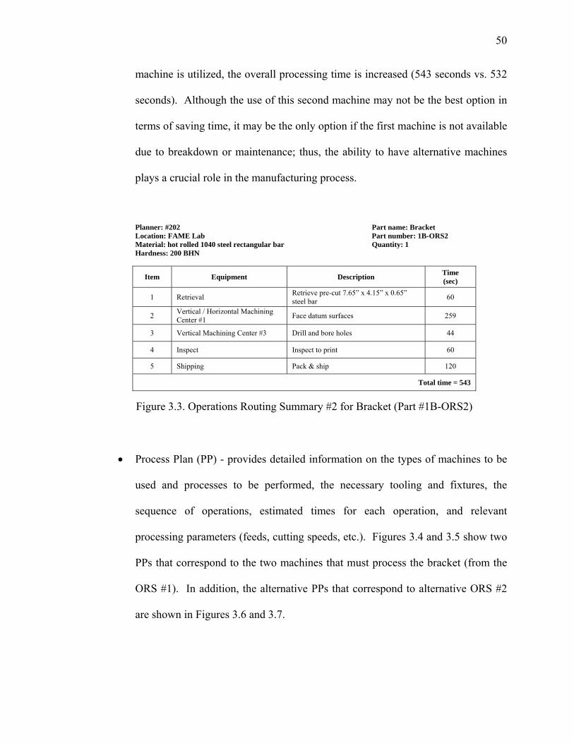
50
machine is utilized, the overall processing time is increased (543 seconds vs. 532
seconds). Although the use of this second machine may not be the best option in
terms of saving time, it may be the only option if the first machine is not available
due to breakdown or maintenance; thus, the ability to have alternative machines
plays a crucial role in the manufacturing process.
Planner: #202 Part name: Bracket Location: FAME Lab Part number: 1B-ORS2 Material: hot rolled 1040 steel rectangular bar Quantity: 1 Hardness: 200 BHN
Item Equipment Description Time (sec)
1 Retrieval Retrieve pre-cut 7.65” x 4.15” x 0.65” steel bar 60
2 Vertical / Horizontal Machining Center #1 Face datum surfaces 259
3 Vertical Machining Center #3 Drill and bore holes 44
4 Inspect Inspect to print 60
5 Shipping Pack & ship 120
Total time = 543
Figure 3.3. Operations Routing Summary #2 for Bracket (Part #1B-ORS2)
• Process Plan (PP) - provides detailed information on the types of machines to be
used and processes to be performed, the necessary tooling and fixtures, the
sequence of operations, estimated times for each operation, and relevant
processing parameters (feeds, cutting speeds, etc.). Figures 3.4 and 3.5 show two
PPs that correspond to the two machines that must process the bracket (from the
ORS #1). In addition, the alternative PPs that correspond to alternative ORS #2
are shown in Figures 3.6 and 3.7.

51
Planner: #202 Part name: Bracket Location: FAME Lab Part number: 1B-ORS1 Material: hot rolled 1040 steel rectangular bar Quantity: 1 Hardness: 200 BHN Process Plan number: 1a Machine: VF-OE
Operation # Description Tooling Velocity, V
(fpm) Feed,
f + Depth of
cut, d (in) Time (sec)#
10 Clamp part on Datum C and C’* Special fixture & automatic clamp 15
20 Face mill Datum A down to 0.5” (2 passes)
2.5” face mill cutter 125 0.012 0.15 92
30 Un-clamp & re-clamp part on Datum A and A’
Special fixture & automatic clamp 25
40 Face mill Datum C down to 4.0” (1 pass)
2.5” face mill cutter 125 0.012 0.15 46
50 Un-clamp & re-clamp part on Datum A and A’
Special fixture & automatic clamp 25
60 Face mill Datum B down to 7.5” (1 pass)
2.5” face mill cutter 125 0.012 0.15 31
70 Un-clamp & re-clamp part on Datum C and C’
Special fixture & automatic clamp 25
Total time = 259 * NOTE: C’ refers to the surface opposite the Datum C surface (A’ and B’ are also opposite surfaces) + feed f : ipr for drilling & boring ; iprpt for milling
Figure 3.4. Process Plan #1a for Bracket (Part #1B-ORS1)
Planner: #202 Part name: Bracket Location: FAME Lab Part number: 1B-ORS1 Material: hot rolled 1040 steel rectangular bar Quantity: 1 Hardness: 200 BHN Process Plan number: 1b Machine: VF-OA
Operation # Description Tooling Velocity, V
(fpm) Feed,
f + Depth of
cut, d (in) Time (sec)#
80 Drill large hole 0.75” Twist drill 85 0.013 0.5 8
90 Quick-change tooling 4
100 Drill small hole 0.4844” Twist drill 80 0.010 0.5 7
110 Quick-change tooling 4
120 Ream hole 0.5” Reamer 45 0.013 0.5 10
Total time = 33 * NOTE: C’ refers to the surface opposite the Datum C surface (A’ and B’ are also opposite surfaces) + feed f : ipr for drilling & boring ; iprpt for milling
Figure 3.5. Process Plan #1b for Bracket (Part #1B-ORS1)

52 Planner: #202 Part name: Bracket Location: FAME Lab Part number: 1B-ORS2 Material: hot rolled 1040 steel rectangular bar Quantity: 1 Hardness: 200 BHN Process Plan number: 2a Machine: VF-OE
Operation # Description Tooling Velocity, V
(fpm) Feed, F +
Depth of cut, d (in)
Time (sec)#
10 Clamp part on Datum C and C’* Special fixture & automatic clamp 15
20 Face mill Datum A down to 0.5” (2 passes)
2.5” face mill cutter 125 0.012 0.15 92
30 Un-clamp & re-clamp part on Datum A and A’
Special fixture & automatic clamp 25
40 Face mill Datum C down to 4.0” (1 pass)
2.5” face mill cutter 125 0.012 0.15 46
50 Un-clamp & re-clamp part on Datum A and A’
Special fixture & automatic clamp 25
60 Face mill Datum B down to 7.5” (1 pass)
2.5” face mill cutter 125 0.012 0.15 31
70 Un-clamp & re-clamp part on Datum C and C’
Special fixture & automatic clamp 25
Total time = 259
Figure 3.6. Process Plan #2a for Bracket (Part #1B-ORS2)
Planner: #202 Part name: Bracket Location: FAME Lab Part number: 1B-ORS2 Material: hot rolled 1040 steel rectangular bar Quantity: 1 Hardness: 200 BHN Process Plan number: 2b Machine: VF-3
Operation # Description Tooling Velocity, V
(fpm) Feed,
f + Depth of
cut, d (in) Time (sec)#
80 Drill large hole 0.75” Twist drill 70 0.012 0.5 11
90 Quick-change tooling 4
100 Drill small hole 0.4844” Twist drill 70 0.009 0.5 9
110 Quick-change tooling 4
120 Bore hole 0.5” Boring bar 120 0.003 0.5 16
Total time = 44
Figure 3.7. Process Plan #2b for Bracket (Part #1B-ORS2)
Generally, PPs are not readily available; thus, processing times in this research is
generated randomly to mimic those that are found in real PPs.

53
• FMC Capability - provides the specifications of a FMC such as programmability
(and re-programmability) of the necessary machines (e.g., robots, CNC machines,
AGVs, etc.), necessary tooling that is capable of supporting a variety of parts or
products, part fixtures (i.e., pallet fixtures) that allow for easy transportation of
parts from one station to another, and system architecture (i.e., the entire network
of equipment and processes that is controlled by a single computer workstation).
3.3. Basic Model Characteristics
When planning these systems, FMS control requirements are very significant aspects to
be considered. In addition, the objective of makespan minimization plays an important
role during this control stage (Shanker and Modi, 1999). This is mainly due to the reality
that jobs usually have tight due dates and arrive at varying times, and there is normally a
requirement to keep the scheduling horizon short. The objective of the basic model for
the FMC scenario considered in this research is to produce a set of sequences over all
machines that minimizes the manufacturing makespan. Details of the model follow in
Section 3.4. The remainder of Section 3.3 articulates underlying model assumptions and
notations.
3.3.1 Assumptions
• All jobs are manufactured at the same facility.
• Raw materials and the tools necessary for production are readily available as
needed since the jobs are processed within a single facility for a specified period.
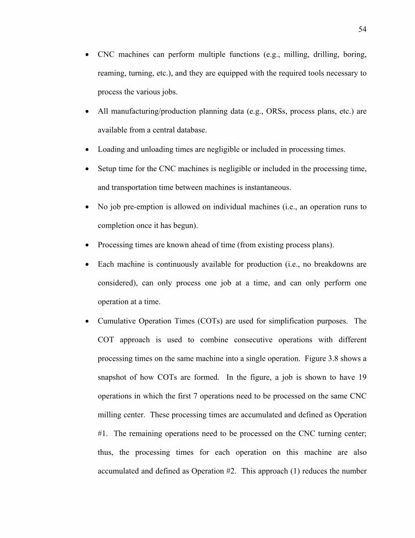
54
• CNC machines can perform multiple functions (e.g., milling, drilling, boring,
reaming, turning, etc.), and they are equipped with the required tools necessary to
process the various jobs.
• All manufacturing/production planning data (e.g., ORSs, process plans, etc.) are
available from a central database.
• Loading and unloading times are negligible or included in processing times.
• Setup time for the CNC machines is negligible or included in the processing time,
and transportation time between machines is instantaneous.
• No job pre-emption is allowed on individual machines (i.e., an operation runs to
completion once it has begun).
• Processing times are known ahead of time (from existing process plans).
• Each machine is continuously available for production (i.e., no breakdowns are
considered), can only process one job at a time, and can only perform one
operation at a time.
• Cumulative Operation Times (COTs) are used for simplification purposes. The
COT approach is used to combine consecutive operations with different
processing times on the same machine into a single operation. Figure 3.8 shows a
snapshot of how COTs are formed. In the figure, a job is shown to have 19
operations in which the first 7 operations need to be processed on the same CNC
milling center. These processing times are accumulated and defined as Operation
#1. The remaining operations need to be processed on the CNC turning center;
thus, the processing times for each operation on this machine are also
accumulated and defined as Operation #2. This approach (1) reduces the number
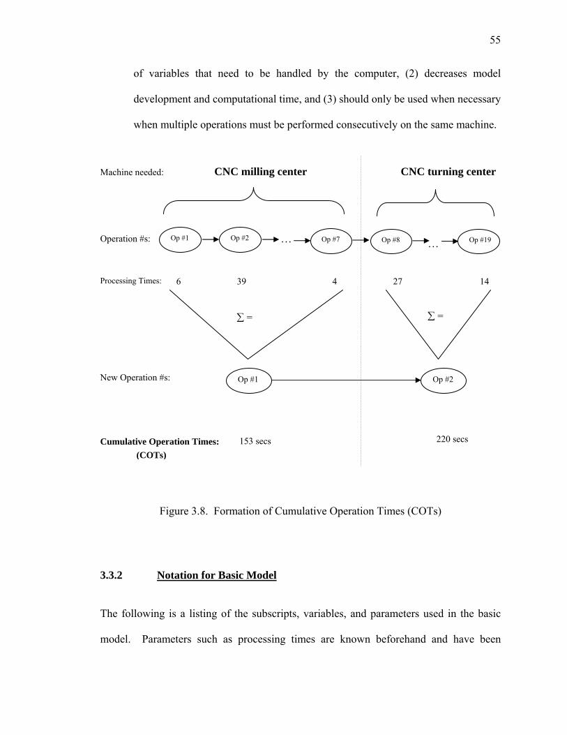
55
(COTs)
of variables that need to be handled by the computer, (2) decreases model
development and computational time, and (3) should only be used when necessary
when multiple operations must be performed consecutively on the same machine.
Machine needed: CNC milling center CNC turning center
Operation #s:
Processing Times:
New Operation #s:
Cumulative Operation Times:
Figure 3.8. Formation of Cumulative Operation Times (COTs)
3.3.2 Notation for Basic Model
The following is a listing of the subscripts, variables, and parameters used in the basic
model. Parameters such as processing times are known beforehand and have been
153 secs
… … Op #1 Op #2 Op #7 Op #8 Op #19
6 39 4 27 14
Op #1 Op #2
220 secs
∑ = ∑ =

56
randomly generated or extracted from given process plans similar to those previously
discussed in Section 3.2.
Subscripts
i or g = 1, 2, ...., N, index for a job in the FMC, where N is the total number of jobs.
j or h = 1, 2, ...., J(i), index for processing operations in the FMC, where J(i) is the final
operation of job i, i = 1, 2, …, N.
k = 1, 2, ...., M, index for a machine in the FMC, where M is the total number of
machines.
Mij (or Mgh) = set of valid optional machines for operation j of job i, j = 1, 2, …, J(i); i =
1, 2, …, N. For example, M32 = {1, 3} denotes that the second operation of job 3
can be performed on either machine 1 or machine 3.
Variables and Parameters
Bij = manufacturing starting time of operation j of job i, j = 1, 2, …, J(i); i = 1, 2, …, N.
Pijk = manufacturing processing time required for operation j of job i on machine k,
j = 1, 2, …, J(i); i = 1, 2, …, N; k = 1, 2, …, M.
γ = large positive integer value used in the disjunctive constraints which help to order
jobs which use the same machine into a specific sequential order.
Xijk = ⎩⎨⎧
otherwise,0, , machineon performed is job of operation if1, kij
k ∈ Mij, Mij : i = 1, 2, …, N; j = 1, 2, …, J(i).

57
Yijghk = ⎪⎩
⎪⎨
⎧
otherwise,0, ,machine sameon the
job of operation beforeperformed is job of operation if1,k
ghij
i ≠ g; k ∈ Mij ∩ Mgh, Mij : i = 1, 2, …, N; j = 1, 2, …, J(i); Mgh : g = 1, 2, …, N;
h = 1, 2, …, J(g).
Ri = ready time of job i.
MS = max {Ci : i = 1, 2, …, N}, makespan is defined as the maximum completion time of
all jobs.
3.4. Detailed Description of Basic 0-1 MILP Model
A MILP model is developed for routing and sequencing a set of N jobs over a limited set
of M machines in a FMC. The model was formulated under the assumptions presented in
Section 3.3.1, and the details of the model are described in the subsequent sections.
3.4.1 Makespan Objective Function
The objective in this model is to minimize the manufacturing completion time or
makespan (MS) for processing all jobs of a batch (or an order). Mathematically, the
problem of minimizing the manufacturing makespan is equivalent to the following
formulation:
Min MS = f(Pijk) (3.1)

58
3.4.2 Constraints
,1, +∈
≤+ ∑ jiMk
ijkijkij BXPBij
i = 1, 2, …, N; j = 1, 2, …, J(i)-1. (3.2)
Constraint set (3.2) ensures that an operation j+1 cannot start before the previous
operation j of the same job i has been completed.
,0)(
)()()(, ≤−+ ∑∈
MSXPBiiJMk
kiiJkiiJiJi i = 1, 2, …, N. (3.3)
Constraint set (3.3) ensures that the starting time and processing time of the last operation
J(i) for job i, i = 1, 2, …, N is less than or equal to the makespan (MS).
,1=∑∈ ijMk
ijkX i = 1, 2, …, N; j = 1, 2, …, J(i). (3.4)
Equations (3.4) ensure that one operation j of job i can only be performed on only one
machine k at a time. In essence, this constraint guarantees that each job i takes only one
path through the system.
,1 ghijkijghkijkghk YYXX +≤−+ (3.5)
i = 1, 2, …, N; g = 1, 2, …, N; i ≠ g; j = 1, 2, …, J(i);
h = 1, 2, …, J(g); k ∈ Mij ∩ Mgh.
Constraint set (3.5) restricts two operations of two different jobs that are scheduled on the
same machine from being performed at the same time. Thus, only one operation of one
job is always performed before the other operation of the second job.

59
,1≤+ ghijkijghk YY (3.6)
i = 1, 2, …, N; g = 1, 2, …, N; i ≠ g; j = 1, 2, …, J(i);
h = 1, 2, …, J(g); k ∈ Mij ∩ Mgh.
,)1()()( ijkijkghijkghkghkghijkijkij XPYXPBXPB ≥−++−+ γ (3.7)
i = 1, 2, …, N; g = 1, 2, …, N; i ≠ g; j = 1, 2, …, J(i);
h = 1, 2, …, J(g); k ∈ Mij ∩ Mgh.
,)1()()( ghkghkijghkijkijkijghkghkgh XPYXPBXPB ≥−++−+ γ (3.8)
i = 1, 2, …, N; g = 1, 2, …, N; i ≠ g; j = 1, 2, …, J(i);
h = 1, 2, …, J(g); k ∈ Mij ∩ Mgh.
Constraint set (3.6) guarantees that if operations j and h from jobs i and g, respectively,
are to be performed on the same machine k, then the two operations can not be performed
simultaneously. Constraint set (3.7) ensures that if operation j of job i is chosen to be
processed before operation h of job g, the starting time and processing time of operation j
of job i must be less than the starting time of operation h of job g. The same logic applies
to constraint set (3.8) for the reverse case when operation h of job g is chosen to be
processed before operation j of job i. Again, these constraints reinforce that one job is
always processed before a second job on a given machine to avoid conflicts.
,1 ii RB ≥ i = 1, 2, …, N. (3.9)

60
Constraint set (3.9) ensures that the first operation of a job i cannot start before it is
ready.
,0≥ijB i = 1, 2, …, N; j = 2, …, J(i). (3.10)
,0≥MS (3.11)
Non-negativity constraints (3.10) and (3.11) ensure that all starting times for the
remaining operations and the manufacturing makespan are positive.
Xijk ∈ {0,1}, i = 1, 2, …, N; j = 1, 2, …, J(i); k = 1, 2, …, M. (3.12)
Yijghk ∈ {0,1}, i = 1, 2, …, N; j = 1, 2, …, J(i); g = 1, 2, …, N; (3.13)
h = 1, 2, …, J(g); k = 1, 2, …, M.
Constraints (3.12) and (3.13) show the integer constraints for the 0-1 variables.
3.4.3 Example Problem
A simple example of the proposed formulation is presented next. In Table 3.1, sample
data that was randomly generated using Microsoft Excel is given. The processing times
and due dates have been generated from integer uniform distributions between 1 and 2,
and between 3 and 6, respectively. This data represents the processing times and
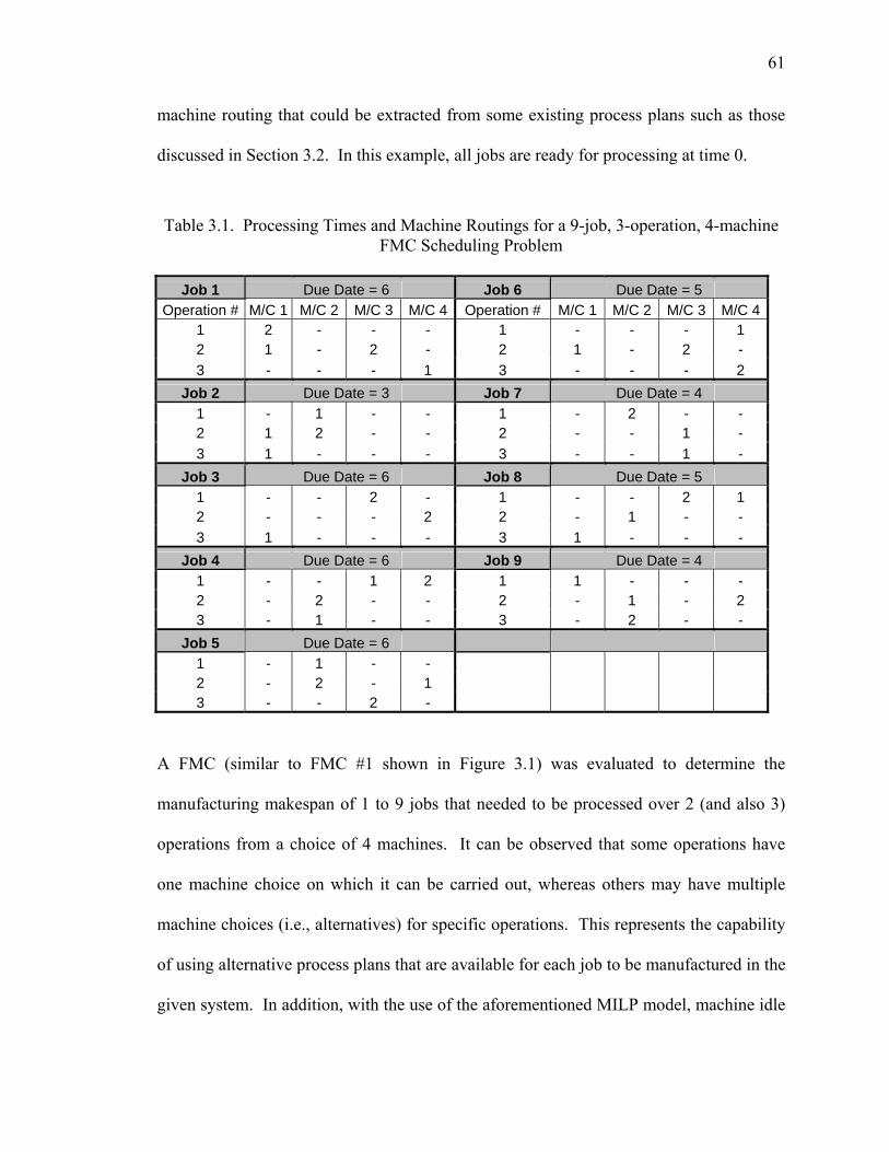
61
machine routing that could be extracted from some existing process plans such as those
discussed in Section 3.2. In this example, all jobs are ready for processing at time 0.
Table 3.1. Processing Times and Machine Routings for a 9-job, 3-operation, 4-machine FMC Scheduling Problem
Job 1 Due Date = 6 Job 6 Due Date = 5
Operation # M/C 1 M/C 2 M/C 3 M/C 4 Operation # M/C 1 M/C 2 M/C 3 M/C 41 2 - - - 1 - - - 1 2 1 - 2 - 2 1 - 2 - 3 - - - 1 3 - - - 2
Job 2 Due Date = 3 Job 7 Due Date = 4 1 - 1 - - 1 - 2 - - 2 1 2 - - 2 - - 1 - 3 1 - - - 3 - - 1 -
Job 3 Due Date = 6 Job 8 Due Date = 5 1 - - 2 - 1 - - 2 1 2 - - - 2 2 - 1 - - 3 1 - - - 3 1 - - -
Job 4 Due Date = 6 Job 9 Due Date = 4 1 - - 1 2 1 1 - - - 2 - 2 - - 2 - 1 - 2 3 - 1 - - 3 - 2 - -
Job 5 Due Date = 6 1 - 1 - - 2 - 2 - 1 3 - - 2 -
A FMC (similar to FMC #1 shown in Figure 3.1) was evaluated to determine the
manufacturing makespan of 1 to 9 jobs that needed to be processed over 2 (and also 3)
operations from a choice of 4 machines. It can be observed that some operations have
one machine choice on which it can be carried out, whereas others may have multiple
machine choices (i.e., alternatives) for specific operations. This represents the capability
of using alternative process plans that are available for each job to be manufactured in the
given system. In addition, with the use of the aforementioned MILP model, machine idle

62
time is reduced while the actual routing and sequencing of the operations are efficiently
performed.
3.4.4 Problem Characterization
To illustrate the computational requirements of the exact mathematical programming
(MP) model using an optimization software package, the 0-1 MILP model presented in
Section 3.4.1 was tested using LP_Solve 5.5 (Berkelaar et al., 2004) on a Pentium 4
2.0GHz computer workstation. The sample data from Table 3.1 was run and evaluated
with the 0-1 MILP model for a total of 18 test case problems in two trial runs: Run #1
used only the first two operations of each job for the test case problems where N ranged
from 1 to 9 jobs, while Run #2 used all three operations of each job for the test case
problems where N ranged from 1 to 9 jobs. Thus, the total number of test cases problems
was 18. The results from these trial runs are presented in Table 3.2 and Table 3.3.
Table 3.2. Run #1 - Makespan Results with 4 Machines and 2 Operations for 9 Jobs
Jobs, N
Operations, J(i)
Machines, M
Number of
Variables
Number of Integer Variables
Number of Constraints
Best Objective (Solution)
CPU Runtime (seconds)
1 2 4 10 2 4 3 0.015 2 2 4 23 8 16 3 0.015 3 2 4 32 10 23 4 0.015 4 2 4 51 22 47 4 0.031 5 2 4 76 40 83 5 0.093 6 2 4 103 60 123 5 0.391 7 2 4 128 78 162 6 5.0638 8 2 4 167 110 226 7 241.219 9 2 4 208 144 294 7 1375.656

63
Table 3.3. Run #2 - Makespan Results with 4 Machines and 3 Operations for 9 Jobs
Jobs, N
Operations, J(i)
Machines, M
Number of
Variables
Number of
Integer Variables
Number of Constraints
Best Objective (Solution)
CPU Runtime (seconds)
1 3 4 13 2 5 4 0.016 2 3 4 33 12 26 4 0.015 3 3 4 55 24 54 5 0.031 4 3 4 83 42 91 5 0.047 5 3 4 123 72 152 6 0.188 6 3 4 169 108 225 7 4.297 7 3 4 211 140 293 7 22.281 8 3 4 402 194 402 8 985.890 9 3 4 347 256 527 11* 36029.750
* = non-optimal solution; user stopped once 10 hours was reached
For each test case problem, these tables show the following information: number of jobs,
number of operations, number of machines, number of variables, number of integer
variables, number of constraints generated, best makespan solution found, and total CPU
runtime. Several test cases were verified for correctness by examining the data from the
LP_Solve output files and plotting Gantt charts to ensure that the final starting time and
makespan parameters were accurate. In addition, LP_Solve has several built-in basis
factorization packages that ensure optimization accuracy. As observed, the nine test case
problems in Run #1 have a range of 2 to 144 integer variables and 4 to 294 total
constraints. The largest problem with 9 jobs and 2 operations had an optimal solution of
7 time units, which was achieved in 1375.656 seconds (22 min, 55.656 sec). It can be
noted here that there is a significant difference in CPU runtime between 7 jobs to 9 jobs;
thus, it is most likely that the CPU runtime will continue to grow exponentially as the
number of jobs are increased. A graphical representation of Run #1 which shows the
CPU runtime compared with the number of jobs is presented in Figure 3.9.
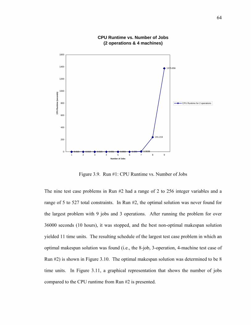
64
CPU Runtime vs. Number of Jobs(2 operations & 4 machines)
0.015 0.015 0.015 0.031 0.093 0.391 5.0638
241.219
1375.656
0
200
400
600
800
1000
1200
1400
1600
1 2 3 4 5 6 7 8 9
Number of Jobs
CPU
Run
time
(sec
onds
)
CPU Runtime for 2 operations
Figure 3.9. Run #1: CPU Runtime vs. Number of Jobs
The nine test case problems in Run #2 had a range of 2 to 256 integer variables and a
range of 5 to 527 total constraints. In Run #2, the optimal solution was never found for
the largest problem with 9 jobs and 3 operations. After running the problem for over
36000 seconds (10 hours), it was stopped, and the best non-optimal makespan solution
yielded 11 time units. The resulting schedule of the largest test case problem in which an
optimal makespan solution was found (i.e., the 8-job, 3-operation, 4-machine test case of
Run #2) is shown in Figure 3.10. The optimal makespan solution was determined to be 8
time units. In Figure 3.11, a graphical representation that shows the number of jobs
compared to the CPU runtime from Run #2 is presented.

65
8 Jobs, 3 Operations, 4 M/Cs Machine 1 P111 P121 P221 P231 P621 P331 P831 Machine 2 P212 P512 P422 P712 P822 P432 Machine 3 P413 P313 P533 P723 P733 Machine 4 P614 P814 P524 P134 P324 P634 0 1 2 3 4 5 6 7 8
Time (seconds)
Figure 3.10. Optimal Makespan Schedule for an 8-job, 3-operation, 4-machine FMC Scheduling Problem (derived from Table 3.1)
CPU Runtime vs. Number of Jobs(3 operations & 4 machines)
0.016 0.015 0.031 0.047 0.188 4.297 22.281985.89
36029.75
0
5000
10000
15000
20000
25000
30000
35000
40000
1 2 3 4 5 6 7 8 9
Number of Jobs
CPU
Run
time
(sec
onds
)
CPU Runtime for 3 operations
Figure 3.11. Run #2: CPU Runtime vs. Number of Jobs
66
In reality these problems are not very large in terms of number of jobs, but the increasing
number of integer variables makes them very difficult to solve in a timely manner. This
increase is due mainly to having multiple machine alternatives available for the jobs. For
instance, in the largest integer variable case, the problem required 347 variables (of
which 256 were integer), and 527 constraints. The computer would have to perform 2256
combinations in order to solve this problem.
If it takes over 10 hours to find an optimal solution for this type of problem, it is assumed
that it would probably take an equivalent amount of time or longer for problems with a
greater number of integer variables and constraints just to search for an optimal solution.
In order to perform realistic FMC scheduling in a timely manner, a problem of this
magnitude would prohibit the use of such a MP model and limit its usability from a
practical standpoint.
It is apparent from both Figure 3.9 and Figure 3.11 that the computational requirements
grow exponentially as the problem size increases, which supports the fact that this type of
problem is NP-hard. This dilemma inspired the development of a two-stage heuristic
methodology that is presented in Chapter 4. By developing a two-stage methodology, the
following items can be accomplished immediately:
(1) Provide insight for the formation of an effective heuristic method to be used for
scheduling decisions,

67
(2) Ability to solve the same types of FMC problems or larger sized problems (as
those discussed Section 3.4.3) in a fraction of the time it would normally take for
the exact 0-1 MILP model,
(3) Provide optimal or non-optimal (but very good) solutions for various size FMC
scheduling problems, and
(4) Generate high quality “useful” schedules in a reasonable amount of time for the
FMS environment.
Before presenting the heuristic methodology, a few extensions of the basic model are
presented in the next section. These extensions show the flexibility and robustness of the
overall MILP model structure presented in Section 3.4, and they also lay the foundation
for future research in which this full MILP model framework could be used. In addition,
a two-stage MILP model is presented. This dual model approach is developed with the
idea of trying to solve the FMC routing and scheduling problem more efficiently.
3.5. Extensions of the Basic Model
Unlike a simulation model, a 0-1 MILP formulation is designed to give an optimal
solution, as well as provide a basic understanding and foundation for a given FMS
scheduling problem. Thus, it lends itself to be easily extended to a number of
performance measures that are dependent on what a scheduler needs to resolve for a
specific manufacturing environment. With minimal change to the basic model, some of
the regular performance measures that could be used with this MILP formulation are total

68
completion time, mean completion time, total flowtime, mean flowtime, maximum
lateness, maximum tardiness, or even the number of tardy jobs.
Additionally, another nice characteristic about this MILP model is that it could also be
used to evaluate non-regular performance measures such as minimizing deviations from a
common due date. Normally, when trying to measure conformance to due dates, jobs
that finish late have traditionally been penalized; however, the jobs that complete their
processing early are often overlooked and are not penalized. With increasing global
competition, the Just-In-Time (JIT) philosophy has become a growing interest in recent
times. In this type of scheduling environment, jobs that finish processing early are held
as overstock inventory until they reach their due dates, and the jobs that finish processing
late will get to the customer well beyond an agreed due date. This situation with early
jobs and late jobs is known as the “earliness and tardiness (E/T) penalties” problem
because both types of jobs are penalized. Occasionally, jobs need to be processed
immediately without any interruptions or delays in order to reduce machine idle time.
This is referred to as no-wait (or nondelay) scheduling (Hutchison and Chang, 1990).
In the following sections, the minimum changes that are required to extend this model for
two additional performance measures and one scheduling condition are presented. The
measures to be discussed involve minimizing tardiness (regular performance measure)
and minimizing the absolute deviation of meeting due dates (non-regular performance),
as well as the no-wait scheduling condition. However, before doing so, additional
variables and parameters need to be introduced.

69
3.5.1 Additional Notation for Model Extensions
Ci = manufacturing completion time of job i, i = 1, 2, …, N.
Di = due date of job i, i = 1, 2, …, N.
Ei = max {0, Di - Ci}, the earliness of job i, i = 1, 2, …, N.
Ti = max {0, Ci - Di}, the tardiness of job i, i = 1, 2, …, N.
Tmax = maxi {Ti}, the maximum tardiness.
αi = the unit earliness penalty for job i, where αi > 0, i = 1, 2, …, N.
βi = the unit tardiness penalty for job i, where βi > 0, i = 1, 2, …, N.
3.5.2 Maximum Tardiness Problem
In order to minimize tardiness, due date parameters are required in addition to the
processing times and machine routing information that is usually provided in process
plans. To use the existing basic MILP model (from Section 3.4), the makespan
minimization objective function that was given in (3.1) must be changed to the following:
Min Tmax (3.14)
This represents that the new objective is to minimize the maximum tardiness. In
addition, constraint set (3.3) must be replaced with the following set of constraints:
,)(
)()()(, iMk
kiiJkiiJiJi CXPBiiJ
=+ ∑∈
i = 1, 2, …, N. (3.15)

70
The following additional set of constraints must be added:
,0max ≤−− TDC ii i = 1, 2, …, N. (3.16)
Lastly, constraint (3.11) must be replaced with the following constraint:
.0max ≥T (3.17)
Constraint set (3.15) ensures that the starting time and processing time of the last
operation J(i) for job i, i = 1, 2, …, N is equivalent to the manufacturing completion time,
while constraint set (3.16) ensures that the tardiness of job i, i = 1, 2, …, N is less than or
equivalent to the maximum tardiness. The combination of (3.14), (3.15) and (3.16), that
is the new objective function with the new constraints, will ensure that the maximum
tardiness objective is minimized while (3.17) ensures that the maximum tardiness value
will be nonnegative. An example problem for this regular performance measure can be
found in the Appendix (see Section A.1).
3.5.3 Earliness/Tardiness (E/T) Problem
Very few models address the minimization of absolute deviation of meeting due dates
(i.e., E/T penalties) in a FMS environment. In the literature, flowtime-related measures
have attracted the most attention, followed by tardiness-related measures and utilization
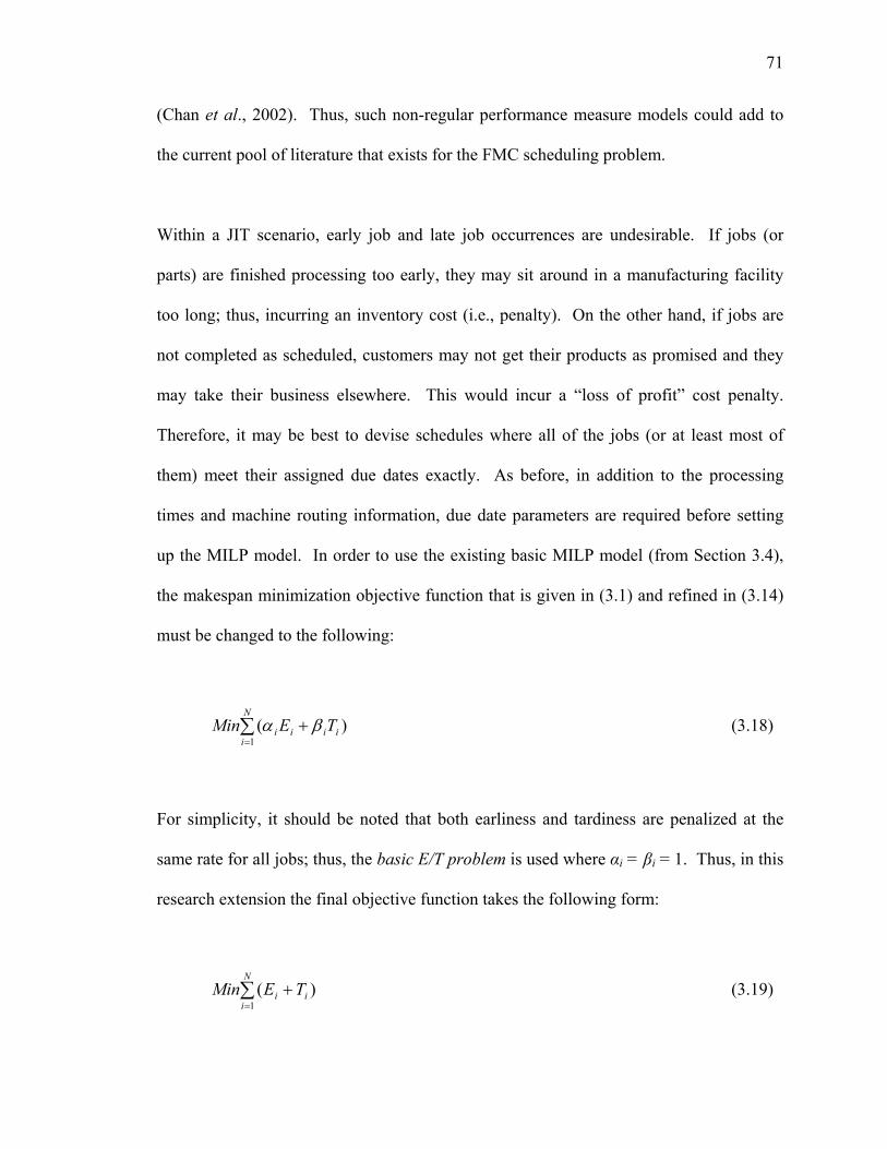
71
(Chan et al., 2002). Thus, such non-regular performance measure models could add to
the current pool of literature that exists for the FMC scheduling problem.
Within a JIT scenario, early job and late job occurrences are undesirable. If jobs (or
parts) are finished processing too early, they may sit around in a manufacturing facility
too long; thus, incurring an inventory cost (i.e., penalty). On the other hand, if jobs are
not completed as scheduled, customers may not get their products as promised and they
may take their business elsewhere. This would incur a “loss of profit” cost penalty.
Therefore, it may be best to devise schedules where all of the jobs (or at least most of
them) meet their assigned due dates exactly. As before, in addition to the processing
times and machine routing information, due date parameters are required before setting
up the MILP model. In order to use the existing basic MILP model (from Section 3.4),
the makespan minimization objective function that is given in (3.1) and refined in (3.14)
must be changed to the following:
∑=
+N
iiiii TEMin
1)( βα (3.18)
For simplicity, it should be noted that both earliness and tardiness are penalized at the
same rate for all jobs; thus, the basic E/T problem is used where αi = βi = 1. Thus, in this
research extension the final objective function takes the following form:
∑=
+N
iii TEMin
1)( (3.19)

72
Additionally, the constraint set denoted in (3.3) must be replaced with (3.15) from
Section 3.5.2.
The following two additional constraints must be added to ensure all jobs i are completed
as close to their due dates as possible (without being too early or too late):
,0≤−− iii ECD i = 1, 2, …, N. (3.20)
,0≤−− iii TDC i = 1, 2, …, N. (3.21)
Lastly, constraint (3.11) must be replaced with the following constraints:
,0≥iE i = 1, 2, …, N. (3.22)
,0≥iT i = 1, 2, …, N. (3.23)
The combination of constraints (3.15), (3.19), (3.20) and (3.21), which represent the new
objective function with the new constraints, ensure that the absolute deviation of meeting
due dates objective is indeed minimized while (3.22) and (3.23) ensure that the earliness
and tardiness values will be nonnegative. Another example problem for this non-regular
performance measure can be found in the Appendix (see section A.3).

73
3.5.4 No-Wait (Non-delay) Scheduling Problem
In a no-wait (or non-delay) scheduling environment, jobs need to be processed without
interruption from start to finish for their assigned sequences. In addition, no machine
should be kept idle for any period of time in which processing could begin on any
subsequent operations. For instance, a job in a bakery may need to travel from one oven
to another while maintaining a specific baking temperature range. Non-delay schedules
are necessary for this type of processing facility and allow the jobs never to undergo
drastic temperature changes, thus allowing the final baked goods to be just right. In order
to achieve these no-wait schedules, constraint set (3.2) must be replaced with the
following constraint:
,1, +∈
=+ ∑ jiMk
ijkijkij BXPBij
i = 1, 2, …, N; j = 1, 2, …, J(i) – 1. (3.24)
Constraint set (3.24) ensures that an operation j+1 must begin immediately on some
downstream machine k after operation j of the same job i has been completed. An
example problem for this special scheduling condition is presented in the Appendix (see
section A.2).
3.6 Two-Stage Routing and Sequencing MILP (2-MILP) Model
Since it has been established earlier that the basic 0-1 MILP model from Section 3.4 is
NP-hard, it is necessary to determine a methodology that can solve the FMC routing and
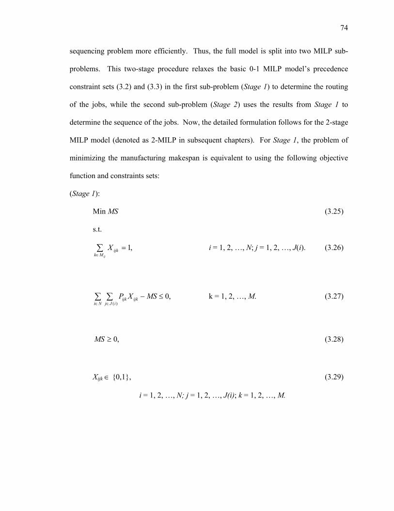
74
sequencing problem more efficiently. Thus, the full model is split into two MILP sub-
problems. This two-stage procedure relaxes the basic 0-1 MILP model’s precedence
constraint sets (3.2) and (3.3) in the first sub-problem (Stage 1) to determine the routing
of the jobs, while the second sub-problem (Stage 2) uses the results from Stage 1 to
determine the sequence of the jobs. Now, the detailed formulation follows for the 2-stage
MILP model (denoted as 2-MILP in subsequent chapters). For Stage 1, the problem of
minimizing the manufacturing makespan is equivalent to using the following objective
function and constraints sets:
(Stage 1):
Min MS (3.25)
s.t.
,1=∑∈ ijMk
ijkX i = 1, 2, …, N; j = 1, 2, …, J(i). (3.26)
,0)(
∑ ∑∈ ∈
≤−Ni iJj
ijkijk MSXP k = 1, 2, …, M. (3.27)
,0≥MS (3.28)
Xijk ∈ {0,1}, (3.29)
i = 1, 2, …, N; j = 1, 2, …, J(i); k = 1, 2, …, M.

75
In this Stage 1 sub-problem, only one new constraint set (3.27) was added. This new
constraint set ensures that for every machine k, which is loaded with selected operations
j ∈ J(i) of jobs i ∈ N, the total processing time on each machine is less than or equal to
the overall makespan. The remaining equations (3.25), (3.26), (3.28) and (3.29) are taken
from the original formulation of the basic 0-1 MILP model from Section 3.4.
Once the Stage 1 model is formulated and solved, the Xijk routing variables are fixed (i.e.,
the routes are fixed for all of the jobs to be processed). The Xijk variables that are
assigned a value of one indicate that operation j of job i is assigned to machine k, while
those assigned a value of zero are not assigned to any machines. Thus, a new subscript
ijM (or ghM ) is introduced where },1:{ˆijijkij MkXkM ∈== . This represents the
selection of the single machine k that is chosen (i.e., the job assigned to the machine) in
Stage 1 from the set of optional machines Mij for operation j of job i. Once this important
information has been established, the Stage 2 sub-problem can now be formulated with
the following objective function and constraint sets:
(Stage 2):
Min MS (3.30)
s.t.
,1, +≤+ jiijkij BPB i = 1, 2, …, N; j = 1, 2, …, J(i)-1; ijMk ˆ∈ . (3.31)
,0),(,)(, ≤−+ MSPB kiJiiJi i = 1, 2, …, N; )(ˆ
iiJMk ∈ . (3.32)
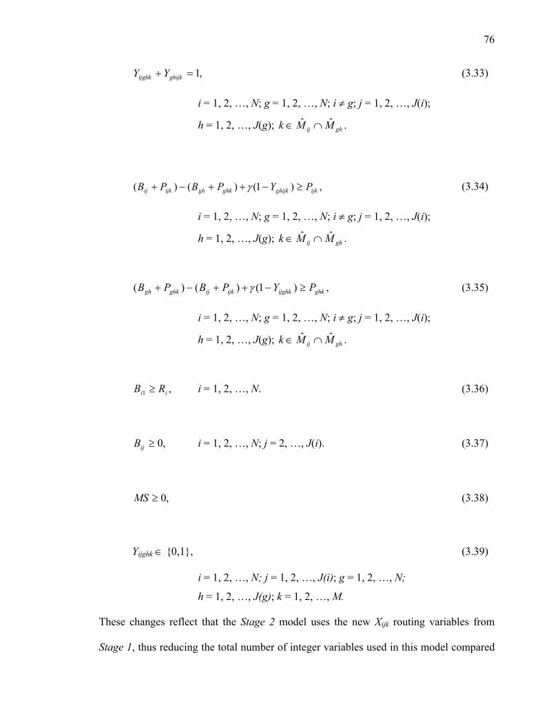
76
,1=+ ghijkijghk YY (3.33)
i = 1, 2, …, N; g = 1, 2, …, N; i ≠ g; j = 1, 2, …, J(i);
h = 1, 2, …, J(g); ghij MMk ˆˆ ∩∈ .
,)1()()( ijkghijkghkghijkij PYPBPB ≥−++−+ γ (3.34)
i = 1, 2, …, N; g = 1, 2, …, N; i ≠ g; j = 1, 2, …, J(i);
h = 1, 2, …, J(g); ghij MMk ˆˆ ∩∈ .
,)1()()( ghkijghkijkijghkgh PYPBPB ≥−++−+ γ (3.35)
i = 1, 2, …, N; g = 1, 2, …, N; i ≠ g; j = 1, 2, …, J(i);
h = 1, 2, …, J(g); ghij MMk ˆˆ ∩∈ .
,1 ii RB ≥ i = 1, 2, …, N. (3.36)
,0≥ijB i = 1, 2, …, N; j = 2, …, J(i). (3.37)
,0≥MS (3.38)
Yijghk ∈ {0,1}, (3.39)
i = 1, 2, …, N; j = 1, 2, …, J(i); g = 1, 2, …, N;
h = 1, 2, …, J(g); k = 1, 2, …, M.
These changes reflect that the Stage 2 model uses the new Xijk routing variables from
Stage 1, thus reducing the total number of integer variables used in this model compared
77
with the amount used in the original 0-1 MILP model. Once Stage 2 has been solved, all
jobs that have been previously routed are now in machine sequences, and a final
makespan value is determined. Some computational results of using this 2-stage MILP
model approach as compared with the original full 0-1 MILP model, and the new
algorithm can be found Chapter 5.
3.7 Concluding Summary
While the makespan performance measure is normally used as a predictive measure, both
performance measures (maximum tardiness and minimum absolute deviation of due dates
presented in Section 3.5) could be used as objective measures as well. For example, if a
machine has a breakdown and a manufacturer already knows that some of the jobs to be
processed are going to be late, these measures could help to determine which jobs should
have more priority in a given batch and sequence. Depending on how late a job may be
beyond its assigned due date, the manufacturer will have the ability to reschedule the
remaining jobs in the FMC, or the actual earliness/tardiness penalties may help to
determine which jobs need to be completed and shipped out of the manufacturing plant
immediately instead of sitting in the plant for some unknown period of time. The non-
delay scheduling condition is always useful if a manufacturer needs to reduce machine
idle time and process jobs in succession without interruption. Again, FMC problems that
utilize these model extensions will require growing computational effort as the number of
jobs increase. Thus, it is best to use the structures of these extended models to develop
efficient methods for solving larger FMC problems. In this research, the major focus is
78
on the makespan performance measure; however, all of the extensions mentioned in this
section are discussed as part of future research.
One efficient method for solving larger FMC problems is to split the full 0-1 MILP
model into two stages. The two-stage routing and sequencing MILP model (2-MILP), as
discussed in Section 3.6., uses the first stage to solve the routing problem, and the second
stage to solve the sequencing problem. Although the 2-MILP model method can solve
problems somewhat faster and slightly larger that the full 0-1 MILP model, this method is
still limited by the size of the problems. To avoid using these limited MILP models, an
efficient algorithm, such as the Tabu Search algorithm (TS Algorithm) presented in the
next chapter, is developed. The TS Algorithm is a method that can solve large problems
efficiently, as well as small and medium size problems.
79
Chapter 4
TWO-STAGE TABU SEARCH ALGORITHM
4.1. Introduction
In medium-to-large size FMC scheduling problems, the computational effort needed to
solve the problem grows tremendously as the number of jobs increases. Several attempts
have been made to address this problem (discussed previously in Chapter 2) using
various heuristic methods and mathematical programming approaches, but usually small
instances of the problem yield the best results when using regular performance measures.
As the problem size increases, the formation of the initial sequences becomes a more
critical component in determining an optimal solution; thus, a very good heuristic
methodology should be used to find these initial sequences. When they are combined
with a meta-heuristic procedure such as Glover’s (1989, 1990) Tabu Search, one could
find optimal/near-optimal solutions for the FMC scheduling problem with a smaller
amount of computational effort. A Two-stage Tabu Search Algorithm (henceforth,
designated as the TS Algorithm) is developed in this research and uses these principles to
solve the FMC scheduling problem more efficiently than using stand-alone MILP
models.
The TS Algorithm contains the following two stages: (1) in Stage I the initial job
sequences are formed, and an initial makespan solution is determined, and (2) in Stage II
the makespan solution is improved (if possible), and the job sequences are modified if an
80
improvement in the solution is found. In the following sections of this chapter, two
heuristics used to assign job operations to machines (i.e., job routing) with example
problems are discussed. Then, a heuristic determine the initial sequences of job
operations and initial makespan is discussed. These heuristics are the components that
are utilized in Stage I of the TS Algorithm. Next, a brief description of Glover’s Tabu
Search methodology follows. Finally, a discussion of the overall TS Algorithm and a full
illustrative example problem using this new algorithm is presented.
4.2. Earliest Completion Time (ECT) Heuristic
An existing greedy heuristic called the earliest completion time (ECT) heuristic
developed by Ibarra and Kim (1977) was utilized to determine initial sequences with
relaxed job precedence constraints. The objective of the heuristic is to schedule N jobs
on M machines so that the maximum completion time Cmax (i.e., the makespan or MS
value) is minimized. This MS value represents the total processing time on the most
heavily loaded machine. Despite its age, this heuristic is one of the few greedy heuristics
used for solving a non-identical (unrelated) M-machine N-job scheduling problem, which
does not require the use of any linear or integer programming techniques.
Since multiple job operations are incorporated, the original job i with operation j will be
called job (i,j) from this point on. In addition, a job (i,j) can be processed on any machine
k in set Mij and processing times Pijk may be different. In this heuristic, the earliest
possible completion time of each unscheduled job is determined, and the job (i,j) that has
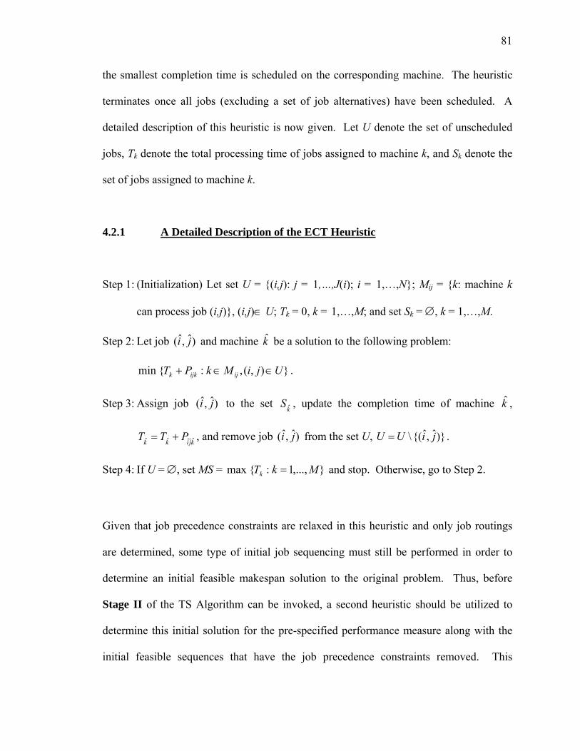
81
the smallest completion time is scheduled on the corresponding machine. The heuristic
terminates once all jobs (excluding a set of job alternatives) have been scheduled. A
detailed description of this heuristic is now given. Let U denote the set of unscheduled
jobs, Tk denote the total processing time of jobs assigned to machine k, and Sk denote the
set of jobs assigned to machine k.
4.2.1 A Detailed Description of the ECT Heuristic
Step 1: (Initialization) Let set U = {(i,j): j = 1,…,J(i); i = 1,…,N}; Mij = {k: machine k
can process job (i,j)}, (i,j)∈ U; Tk = 0, k = 1,…,M; and set Sk = ∅, k = 1,…,M.
Step 2: Let job )ˆ,ˆ( ji and machine k be a solution to the following problem:
}),(,:{min UjiMkPT ijijkk ∈∈+ .
Step 3: Assign job )ˆ,ˆ( ji to the set k
S ˆ , update the completion time of machine k ,
kjikkPTT ˆˆˆˆ += , and remove job )ˆ,ˆ( ji from the set U, )}ˆ,ˆ{(\ jiUU = .
Step 4: If U = ∅, set MS = },...,1:{max MkTk = and stop. Otherwise, go to Step 2.
Given that job precedence constraints are relaxed in this heuristic and only job routings
are determined, some type of initial job sequencing must still be performed in order to
determine an initial feasible makespan solution to the original problem. Thus, before
Stage II of the TS Algorithm can be invoked, a second heuristic should be utilized to
determine this initial solution for the pre-specified performance measure along with the
initial feasible sequences that have the job precedence constraints removed. This

82
heuristic (i.e., the Vancheeswaran-Townsend heuristic) is discussed in Section 4.4. Next,
an illustrative example of the ECT heuristic is shown.
4.2.2 Illustrative Example of the ECT Heuristic
A simple example with randomly generated data is presented in Table 4.1. The
processing times have been generated from integer uniform distributions between 5 and
30. The parameters in Table 4.1 indicate that there are 6 jobs with 3 operations each.
Each operation can be performed on at least 1 of 4 machines. In addition, some
operations can be processed on alternative machines. For example, operation 2 of job 4
can be processed on either machine 1 or machine 4.
Table 4.1. Processing Times and Machine Routings for a 6-job, 3-operation, 4-machine FMC Scheduling Problem
Operation
# M/C
1 M/C
2 M/C
3 M/C
4 Operation #
M/C 1
M/C 2
M/C 3
M/C 4
1 - - 22 - 1 - - - 20 JOB 1 2 5 - - - JOB 4 2 27 - - 19
3 22 - - 26 3 14 - - - 1 18 12 - - 1 18 - - -
JOB 2 2 17 24 - - JOB 5 2 17 25 - - 3 - - - 25 3 - 17 - - 1 - - 17 25 1 - - 21 18
JOB 3 2 16 - - - JOB 6 2 - - - 25 3 16 30 - 3 21 - - -
Each step of the ECT heuristic example problem is outlined as follows:
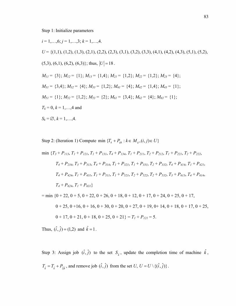
83
Step 1: Initialize parameters
i = 1,…,6; j = 1,…,3; k = 1,…,4.
U = {(1,1), (1,2), (1,3), (2,1), (2,2), (2,3), (3,1), (3,2), (3,3), (4,1), (4,2), (4,3), (5,1), (5,2),
(5,3), (6,1), (6,2), (6,3)}; thus, 18=U .
M11 = {3}; M12 = {1}; M13 = {1,4}; M21 = {1,2}; M22 = {1,2}; M23 = {4};
M31 = {3,4}; M32 = {4}; M33 = {1,2}; M41 = {4}; M42 = {1,4}; M43 = {1};
M51 = {1}; M52 = {1,2}; M53 = {2}; M61 = {3,4}; M62 = {4}; M63 = {1};
Tk = 0, k = 1,…,4 and
Sk = ∅, k = 1,…,4.
Step 2: (Iteration 1) Compute }),(,:{min UjiMkPT ijijkk ∈∈+
min {T3 + P113, T1 + P121, T1 + P131, T4 + P134, T1 + P211, T2 + P212, T1 + P221, T2 + P222,
T4 + P234, T3 + P313, T4 + P314, T1 + P321, T1 + P331, T2 + P332, T4 + P414, T1 + P421,
T4 + P424, T1 + P431, T1 + P511, T1 + P521, T2 + P522, T2 + P532, T3 + P613, T4 + P614,
T4 + P624, T1 + P631}
= min {0 + 22, 0 + 5, 0 + 22, 0 + 26, 0 + 18, 0 + 12, 0 + 17, 0 + 24, 0 + 25, 0 + 17,
0 + 25, 0 +16, 0 + 16, 0 + 30, 0 + 20, 0 + 27, 0 + 19, 0+ 14, 0 + 18, 0 + 17, 0 + 25,
0 + 17, 0 + 21, 0 + 18, 0 + 25, 0 + 21} = T1 + P121 = 5.
Thus, )2,1()ˆ,ˆ( =ji and 1ˆ =k .
Step 3: Assign job )ˆ,ˆ( ji to the set k
S ˆ , update the completion time of machine k ,
kjikkPTT ˆˆˆˆ += , and remove job )ˆ,ˆ( ji from the set U, )}ˆ,ˆ{(\ jiUU = .

84
S1 = {(1,2)}; S2 = ∅; S3 = ∅; S4 = ∅.
T1 = T1 + P121 = 0 + 5; thus, T1 = 5.
)}2,1{(\UU = = {(1,1), (1,3), (2,1), (2,2), (2,3), (3,1), (3,2), (3,3), (4,1), (4,2), (4,3),
(5,1), (5,2), (5,3), (6,1), (6,2), (6,3)}; thus, 17=U .
Since U ≠ ∅, go to Step 2.
Step 2: (Iteration 2) Compute }),(,:{min UjiMkPT ijijkk ∈∈+
min {T3 + P113, T1 + P131, T4 + P134, T1 + P211, T2 + P212, T1 + P221, T2 + P222, T4 + P234,
T3 + P313, T4 + P314, T1 + P321, T1 + P331, T2 + P332, T4 + P414, T1 + P421, T4 + P424,
T1 + P431, T1 + P511, T1 + P521, T2 + P522, T2 + P532, T3 + P613, T4 + P614, T4 + P624,
T1 + P631}
= min {0 + 22, 5 + 22, 0 + 26, 5 + 18, 0 + 12, 5 + 17, 0 + 24, 0 + 25, 0 + 17, 0 + 25,
5 +16, 5 + 16, 0 + 30, 0 + 20, 5 + 27, 0 + 19, 5 + 14, 5 + 18, 5 + 17, 0 + 25,
0 + 17, 0 + 21, 0 + 18, 0 + 25, 5 + 21} = T2 + P212 = 12.
Thus, )1,2()ˆ,ˆ( =ji and 2ˆ =k .
Step 3: Assign job )ˆ,ˆ( ji to the set k
S ˆ , update the completion time of machine k ,
kjikkPTT ˆˆˆˆ += , and remove job )ˆ,ˆ( ji from the set U, )}ˆ,ˆ{(\ jiUU = .
S1 = {(1,2)}; S2 = {(2,1)}; S3 = ∅; S4 = ∅.
T2 = T2 + P212 = 0 + 12; thus, T2 = 12.
)}1,2{(\UU = = {(1,1), (1,3), (2,2), (2,3), (3,1), (3,2), (3,3), (4,1), (4,2), (4,3), (5,1),
(5,2), (5,3), (6,1), (6,2), (6,3)}; thus, 16=U .
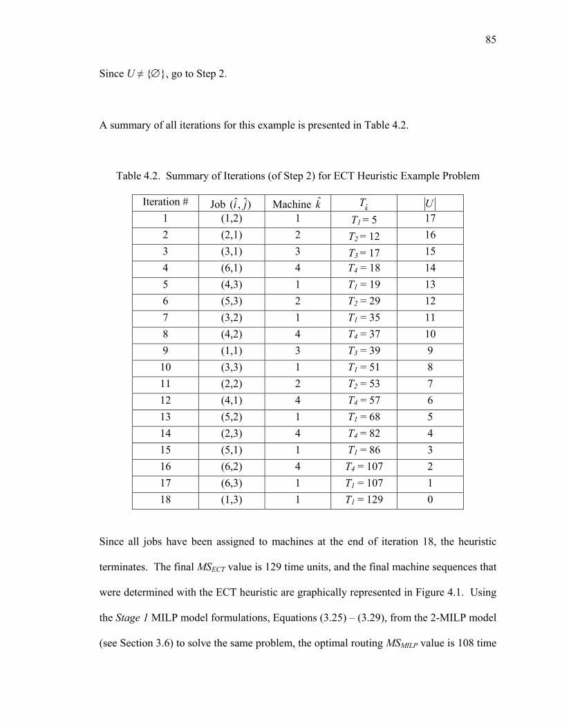
85
Since U ≠ {∅}, go to Step 2.
A summary of all iterations for this example is presented in Table 4.2.
Table 4.2. Summary of Iterations (of Step 2) for ECT Heuristic Example Problem
Iteration # Job )ˆ,ˆ( ji Machine k kT ˆ U
1 (1,2) 1 T1 = 5 17 2 (2,1) 2 T2 = 12 16 3 (3,1) 3 T3 = 17 15 4 (6,1) 4 T4 = 18 14 5 (4,3) 1 T1 = 19 13 6 (5,3) 2 T2 = 29 12 7 (3,2) 1 T1 = 35 11 8 (4,2) 4 T4 = 37 10 9 (1,1) 3 T3 = 39 9 10 (3,3) 1 T1 = 51 8 11 (2,2) 2 T2 = 53 7 12 (4,1) 4 T4 = 57 6 13 (5,2) 1 T1 = 68 5 14 (2,3) 4 T4 = 82 4 15 (5,1) 1 T1 = 86 3 16 (6,2) 4 T4 = 107 2 17 (6,3) 1 T1 = 107 1 18 (1,3) 1 T1 = 129 0
Since all jobs have been assigned to machines at the end of iteration 18, the heuristic
terminates. The final MSECT value is 129 time units, and the final machine sequences that
were determined with the ECT heuristic are graphically represented in Figure 4.1. Using
the Stage 1 MILP model formulations, Equations (3.25) – (3.29), from the 2-MILP model
(see Section 3.6) to solve the same problem, the optimal routing MSMILP value is 108 time
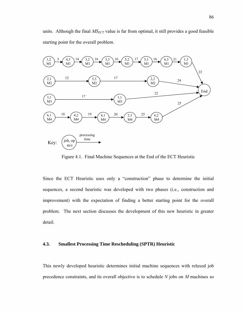
86
units. Although the final MSECT value is far from optimal, it still provides a good feasible
starting point for the overall problem.
Figure 4.1. Final Machine Sequences at the End of the ECT Heuristic
Since the ECT Heuristic uses only a “construction” phase to determine the initial
sequences, a second heuristic was developed with two phases (i.e., construction and
improvement) with the expectation of finding a better starting point for the overall
problem. The next section discusses the development of this new heuristic in greater
detail.
4.3. Smallest Processing Time Rescheduling (SPTR) Heuristic
This newly developed heuristic determines initial machine sequences with relaxed job
precedence constraints, and its overall objective is to schedule N jobs on M machines so
17 5 1,2 M1
job, op m/c
processing time
Key:
6,3 M1
4,1 M4
3,2 M1
6,2 M4
2,3 M4
3,3 M1
5,2 M1
22
20
16
25
16 5,1 M1
End
18 6,1 M4
4,2 M4
17 3,1 M3
1,1 M3
22
12 2,1 M2
5,3 M2
2,2 M2
1,3 M1
17 24
25
18
19
4,3 M1
14 21

87
that the maximum completion time Cmax (i.e., the makespan MS value) is minimized. As
designated in the previous section, a job (i,j) can be processed on any machine k in set
Mij. Processing times, Pijk, are associated with each job and they may be different since
one or more operations of the job can be performed on another machine k’ in set Mij.
Generally, the SPTR Heuristic is comprised of two phases – a construction phase and an
improvement phase. In this heuristic, unscheduled jobs are initially assigned to machines
based on their smallest processing time values and an initial MS value is determined
during the construction phase. After this preliminary assignment of jobs to machines is
performed, the improvement phase attempts to improve the MS value during each
iteration by moving a job (i,j) previously assigned to a bottleneck machine k to an
alternative machine k’∈ Mij when slack time is greater than Pijk’. Henceforth, this
procedure is denoted as MOVE. When MOVE improves the makespan value with
respect to machines k and k’, the overall makespan value is updated. This MOVE
process repeats until no improvement in the solution is found.
Next, the improvement phase attempts to improve the MS once more by switching a pair
of jobs )ˆ,ˆ( ji and (i’,j’). Hereafter, this procedure is designated as SWITCH. Job )ˆ,ˆ( ji
is moved from the bottleneck machine k to an alternative machine k’, and job (i’,j’) is
moved from an alternative machine k’ to the bottleneck machine k . When SWITCH
improves the makespan value with respect to machines k and k’, the overall makespan
value is updated once again. This entire process repeats (i.e., re-starting with MOVE)
until no improvement in the solution is found, and then the heuristic terminates.
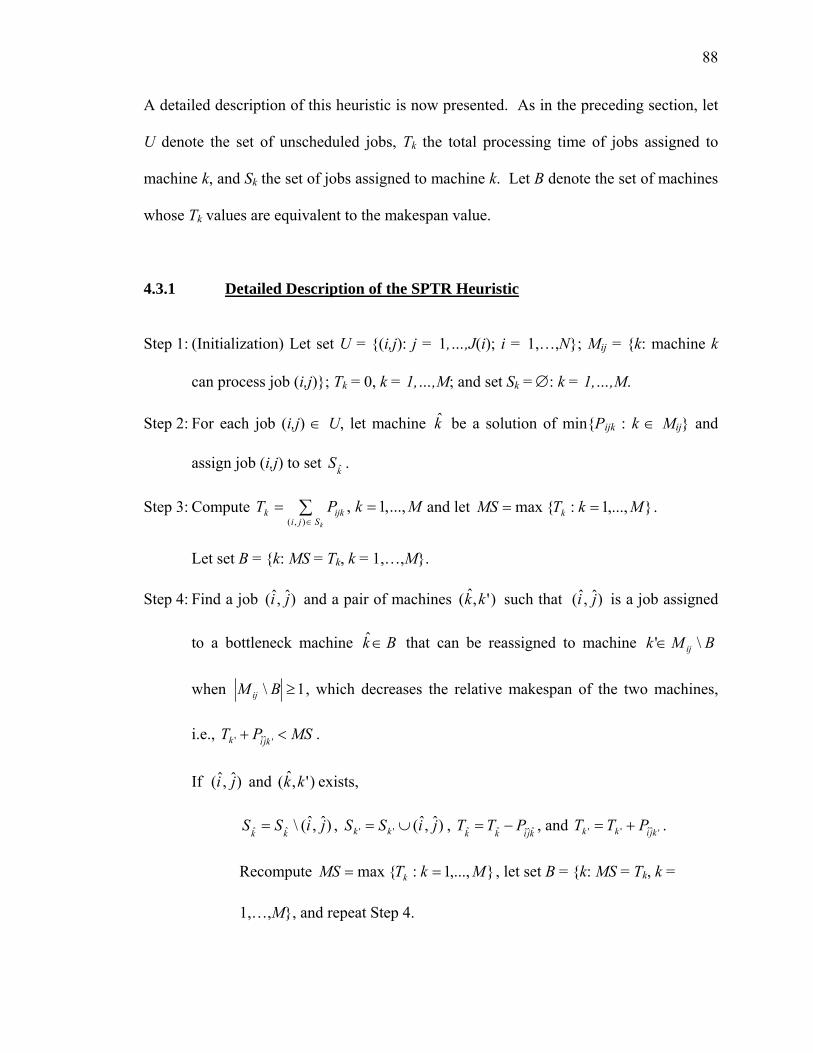
88
A detailed description of this heuristic is now presented. As in the preceding section, let
U denote the set of unscheduled jobs, Tk the total processing time of jobs assigned to
machine k, and Sk the set of jobs assigned to machine k. Let B denote the set of machines
whose Tk values are equivalent to the makespan value.
4.3.1 Detailed Description of the SPTR Heuristic
Step 1: (Initialization) Let set U = {(i,j): j = 1,…,J(i); i = 1,…,N}; Mij = {k: machine k
can process job (i,j)}; Tk = 0, k = 1,…,M; and set Sk = ∅: k = 1,…,M.
Step 2: For each job (i,j) ∈ U, let machine k be a solution of min{Pijk : k ∈ Mij} and
assign job (i,j) to set k
S ˆ .
Step 3: Compute MkPTkSji
ijkk ...,,1,),(
== ∑∈
and let },...,1:{max MkTMS k == .
Let set B = {k: MS = Tk, k = 1,…,M}.
Step 4: Find a job )ˆ,ˆ( ji and a pair of machines )',ˆ( kk such that )ˆ,ˆ( ji is a job assigned
to a bottleneck machine Bk ∈ˆ that can be reassigned to machine BMk ij \'∈
when 1\ ≥BM ij , which decreases the relative makespan of the two machines,
i.e., MSPT kjik <+ 'ˆ' .
If )ˆ,ˆ( ji and )',ˆ( kk exists,
)ˆ,ˆ(\ˆˆ jiSSkk
= , )ˆ,ˆ('' jiSS kk ∪= , kjikk
PTT ˆˆˆˆˆ −= , and 'ˆˆ'' kjikk PTT += .
Recompute },...,1:{max MkTMS k == , let set B = {k: MS = Tk, k =
1,…,M}, and repeat Step 4.

89
Otherwise, goto Step 5.
Step 5: Find a pair of jobs )ˆ,ˆ( ji and (i’,j’) and a pair of machines )',ˆ( kk such that )ˆ,ˆ( ji
is a job assigned to a bottleneck machine Bk ∈ˆ that can be reassigned to machine
BMk ij \'∈ when 1\ ≥BM ij , and (i’,j’) is a job assigned to machine BMk ij \'∈
that can be reassigned to machine Bk ∈ˆ , all while decreasing the relative
makespan of the two machines, i.e., MSPPTkjikjik
<+− ˆ''ˆˆˆ and
MSPPT kjikjik <+− 'ˆ'''' .
If )ˆ,ˆ( ji , (i’,j’), and )',ˆ( kk exists,
)''()]ˆ,ˆ(\[ ˆˆ jijiSSkk
∪= , )ˆ,ˆ()]''(\[ '' jijiSS kk ∪= , kjikjikk
PPTT ˆ''ˆˆˆˆˆ +−= ,
and 'ˆˆ''''' kjikjikk PPTT +−= . Recompute },...,1:{max MkTMS k == , let set
B = {k: MS = Tk, k = 1,…,M}, and repeat Step 4.
Otherwise, stop.
Theorem: The SPTR algorithm terminates in a finite number of iterations.
Proof: At each execution of Step 4 and Step 5 either the cardinality of B decreases by 1
or MS decreases. Since B is a subset of a finite number of machines, the cardinality of B
can only decrease a finite number of times for a given MS value. Since MS is always the
sum of a finite number of processing times and the number of jobs is finite, MS can only
decrease a finite number of times. Therefore, this algorithm must terminate in a finite
number of iterations.
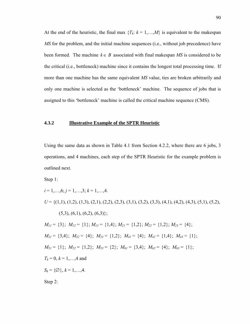
90
At the end of the heuristic, the final max {Tk: k = 1,…,M} is equivalent to the makespan
MS for the problem, and the initial machine sequences (i.e., without job precedence) have
been formed. The machine Bk ∈ associated with final makespan MS is considered to be
the critical (i.e., bottleneck) machine since it contains the longest total processing time. If
more than one machine has the same equivalent MS value, ties are broken arbitrarily and
only one machine is selected as the ‘bottleneck’ machine. The sequence of jobs that is
assigned to this ‘bottleneck’ machine is called the critical machine sequence (CMS).
4.3.2 Illustrative Example of the SPTR Heuristic
Using the same data as shown in Table 4.1 from Section 4.2.2, where there are 6 jobs, 3
operations, and 4 machines, each step of the SPTR Heuristic for the example problem is
outlined next.
Step 1:
i = 1,…,6; j = 1,…,3; k = 1,…,4.
U = {(1,1), (1,2), (1,3), (2,1), (2,2), (2,3), (3,1), (3,2), (3,3), (4,1), (4,2), (4,3), (5,1), (5,2),
(5,3), (6,1), (6,2), (6,3)};
M11 = {3}; M12 = {1}; M13 = {1,4}; M21 = {1,2}; M22 = {1,2}; M23 = {4};
M31 = {3,4}; M32 = {4}; M33 = {1,2}; M41 = {4}; M42 = {1,4}; M43 = {1};
M51 = {1}; M52 = {1,2}; M53 = {2}; M61 = {3,4}; M62 = {4}; M63 = {1};
Tk = 0, k = 1,…,4 and
Sk = {∅}, k = 1,…,4.
Step 2:

91
S1 = {(1,2), (1,3), (2,2), (3,2), (3,3), (4,3), (5,1), (5,2), (6,3)}
S2 = {(2,1), (5,3)}
S3 = {(1,1), (3,1)}
S4 = {(2,3), (4,1), (4,2), (6,1), (6,2)}
Step 3:
T1 = 146, T2 = 29, T3 = 39, T4 = 107;
MS = max {T1, T2, T3, T4} = T1 = 146;
B = {1}.
A graphical representation of these initial starting sequences is shown in Figure 4.2.
Figure 4.2. Initial Starting Machine Sequences
17 18 5 1,2 M1
job, op m/c
processing time
Key:
1,3 M1
2,2 M1
3,2 M1
5,2 M1
3,3 M1
4,3 M1
5,1 M1
22 17 16 16 14 6,3 M1
End
12 2,1 M2
5,3 M2
22 1,1 M3
3,1 M3
17
25 2,3 M4
4,1 M4
4,2 M4
6,1 M4
6,2 M4
20 19 18
25
21
17

92
Step 4. (Iteration 1)
Job (1,3) and machines (1,4) are identified: i = 1, j = 3, k = 1, k’ = 4.
Since T4 + P134 = 107 + 26 = 133 < 146, reschedule the job (update the values).
S1 = S1 \{(1,3)} = {(1,2), (2,2), (3,2), (3,3), (4,3), (5,1), (5,2), (6,3)};
S4 = )}3,1{(4 ∪S = {(2,3), (4,1), (4,2), (6,1), (6,2), (1,3)};
T1 = T1 – P131 = 146 – 22 = 124;
T4 = T4 + P134 = 107 + 26 = 133;
MS = max {T1, T2, T3, T4} = T4 = 133;
B = {4}. Repeat Step 4.
Step 4. (Iteration 2)
Job (4,2) and machines (4,1) are identified: i = 4, j = 2, k = 4, k’ = 1.
Since T1 + P421 = 124 + 27 > 133, do not reschedule the job and search for another job.
Job (6,1) and machines (4,3) are identified: i = 6, j = 1, k = 4, k’ = 3.
Since T3 + P613 = 39 + 21 = 60 < 133, reschedule the job (update the values).
S4 = S4 \{(6,1)} = {(2,3), (4,1), (4,2), (6,2), (1,3)};
S3 = )}1,6{(3 ∪S = {(1,1), (3,1), (6,1)};
T4 = T4 – P614 = 133 – 18 = 115;
T3 = T3 + P613 = 39 + 21 = 60;
MS = max {T1, T2 ,T3 ,T4} = T4 = 115.
B = {4}. Repeat Step 4.
All iterations for this example are summarized in Table 4.3.

93
Table 4.3. Summary of Iterations (of Step 4 & 5) for SPTR Heuristic Example Problem
Iteration # )ˆ,ˆ( ji )','( ji )',ˆ( kk kT ˆ 'kT MS
B
Initialization (Step 1 – 3) - - - - - 146 {1}
1 (Step 4) (1,3) - (1,4) T1 = 124 T4 = 133 133 {4}
2 (Step 4) (6,1) - (4,3) T4 = 115 T3 = 60 124 {1}
3 (Step 4) (2,2) - (1,2) T1 = 107 T2 = 53 115 {4}
4 (Step 4) - - - - - 115 {4}
5 (Step 5) - - - - - 115 {4}
In Iteration 3, MOVE (Step 4) is performed and job (2,2) is removed from Machine 1 and
placed on Machine 2. Machine 4 remains as the bottleneck machine with a makespan
value of 115. In Iteration 4, MOVE (Step 4) is performed once more and two jobs in this
CMS were identified as possible move candidates (i.e., they had alternative machine
choices). Neither job (4,2) nor job (1,3) could move (be rescheduled) from the bottleneck
Machine 4 to another machine since these moves did not improve the makespan value.
Finally, in Iteration 5, an attempt was made to SWITCH jobs (Step 5). No jobs on the
bottleneck Machine 4 could switch with another job on another machine. The empty
column 3 of Table 4.3 indicates that no switch of jobs was made during this particular
problem; thus, all jobs have been assigned to the machines at this point, and the heuristic
stops with a final MSSPTR value of 115 time units. This final MSSPTR value is much closer
to the optimal routing MSMILP value of 108 time units when compared with the final

94
1,2 M1
6,3 M1
2,2 M2
3,2 M1
3,3 M1
4,3 M1
5,1 M1
End
2,1 M2
5,3 M2
1,1 M3
3,1 M3
2,3 M4
4,1 M4
4,2 M4
6,1 M3
6,2 M4
5,2 M1
1,3 M4
MSECT value of 129 time units. The final machine sequences that were determined with
the SPTR Heuristic are graphically represented in Figure 4.3.
Figure 4.3. Final Machine Sequences at the End of the SPTR Heuristic
4.3.3 Computational Study: Routing MILP vs. ECT vs. SPTR
The routing MILP (henceforth, denoted as r-MILP) model formulation from Section 3.6
was coded and solved using LP_Solve 5.5, and both heuristics (ECT and SPTR) were
coded using Microsoft Visual C++ .NET. All problems were tested on a Pentium 4
2.0GHz PC. Since no sample problems have been found in the literature to be used as a
benchmark for testing the heuristics, a total of 27 test problems have been generated
randomly in three data sets as follows. The size of each test problem is represented by
the number of jobs (NJ) and the number of machines (NM), where the number of jobs
ranges between 5 and 140. Each job had 3 operations (NO) and these operations could be
processed on at least 1 of 4 total machines. Processing times were generated from an
19 25
16 14 5
job, op m/c
processing time
Key:
21
24
16
12
22 17
20
21
26
18
17
17
25

95
integer uniform distribution between 5 and 30. The results are summarized in Table 4.4.
For each test problem, that table shows the following information: number of jobs (NJ),
number of operations (NO), number of machines (NM), average makespan values,
average CPU runtime values and average relative errors (Avg. RE) for the ECT and
SPTR Heuristic methods, and the r-MILP model.
Although the ECT Heuristic is good for achieving feasible near-optimal solutions for the
routing sub-problem, it never outperformed the SPTR Heuristic in any of the 27 test
problems as indicated in Table 4.4. All three methods (i.e., ECT Heuristic, SPTR
Heuristic, and the r-MILP model formulation) require little computational effort as noted
in the “Average CPU runtime” columns. However, it should be noted that both the ECT
Heuristic and SPTR Heuristic are much easier to implement than the r-MILP model (i.e.,
running heuristic programs require less effort than formulating and solving entire MP
models). This is especially true for problems with more than 5 jobs because MP models
become very large.
The percent relative error, RE, measures the deviation of the current MS solution, MSECT,
from the best known solution, MSr-MILP, (i.e., the value RE = [ (MSECT - MSr-MILP) /
MSr-MILP] * 100 ). For the examples discussed, three data sets are used to determine the
average percent relative error. Thus, the overall average RE for the ECT Heuristic was
determined to be 11.00%, with the average RE for all jobs ranging from 6.58% to 15.2%.
The ECT Heuristic only found the optimal solution once in Data Set #1 for the case
where N = 5 jobs. The other solutions found were worst.
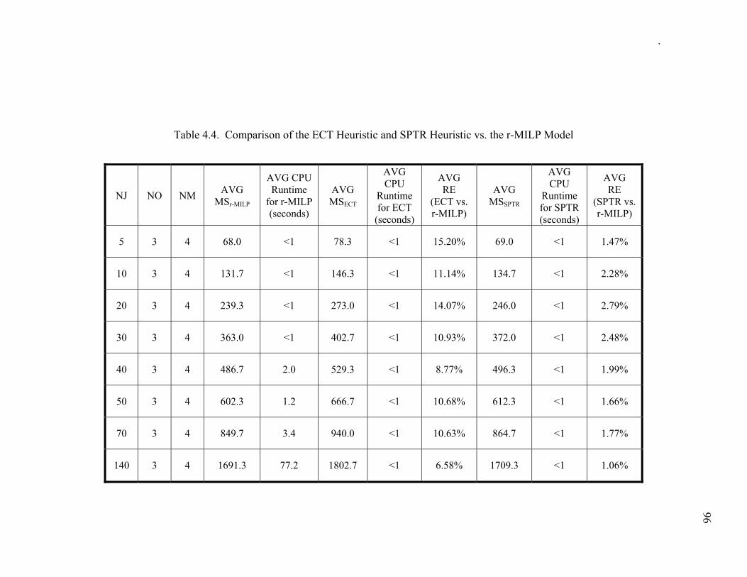
96
Table 4.4. Comparison of the ECT Heuristic and SPTR Heuristic vs. the r-MILP Model
NJ NO NM AVG MSr-MILP
AVG CPU Runtime
for r-MILP (seconds)
AVG MSECT
AVG CPU
Runtime for ECT
(seconds)
AVG RE
(ECT vs. r-MILP)
AVG MSSPTR
AVG CPU
Runtime for SPTR (seconds)
AVG RE
(SPTR vs. r-MILP)
5 3 4 68.0 <1 78.3 <1 15.20% 69.0 <1 1.47%
10 3 4 131.7 <1 146.3 <1 11.14% 134.7 <1 2.28%
20 3 4 239.3 <1 273.0 <1 14.07% 246.0 <1 2.79%
30 3 4 363.0 <1 402.7 <1 10.93% 372.0 <1 2.48%
40 3 4 486.7 2.0 529.3 <1 8.77% 496.3 <1 1.99%
50 3 4 602.3 1.2 666.7 <1 10.68% 612.3 <1 1.66%
70 3 4 849.7 3.4 940.0 <1 10.63% 864.7 <1 1.77%
140 3 4 1691.3 77.2 1802.7 <1 6.58% 1709.3 <1 1.06%
. 96

97
It is better to achieve the optimal (or best near-optimal) solutions during this first segment
(Stage I) of the overall TS Algorithm in hopes of spending less computational time
during Stage II when improvement is necessary. Thus, in order to accomplish this, the
SPTR Heuristic was developed in hopes of making an improvement in the makespan
objective values with respect to the RE. The SPTR Heuristic was tested for the same
three data sets. The test results in Table 4.4 show that this new heuristic performs well
for the given test problems.
The SPTR Heuristic found the optimal solution in only 3 cases, but for the most part, the
solutions were very close to the optimal values found with the routing MILP models.
Comparing the SPTR Heuristic with the routing MILP model, the overall average RE was
determined to be 1.94%, with the average RE for all jobs ranging from 1.1% to 2.8%.
Again, the results in Table 4.4 indicate that this heuristic is an excellent choice for
achieving optimal/near-optimal solutions for the routing sub-problem.
Overall, the SPTR Heuristic performed much better than the ECT Heuristic using the
same test data; therefore, it is the better heuristic for the first segment of Stage I in the TS
Algorithm. Thus, by using this heuristic to find “very good to excellent” initial solutions
during Stage I of the TS Algorithm, less computational time is used during Stage II. The
results from the SPTR Heuristic are used as input for a common job shop scheduling
heuristic developed by Vancheeswaran and Townsend (1993). Henceforth, this heuristic

98
is denoted as the VT Heuristic in this research. Next, a detailed description of the VT
Heuristic is discussed.
4.4. Vancheeswaran-Townsend (VT) Heuristic
The VT Heuristic is a two-phase algorithm that utilizes a network scheduling approach to
determine initial feasible near-optimal sequences of jobs using an urgency criterion in its
first phase, and then improves these sequences during its second phase. However, in this
research, the second phase of the VT Heuristic is not utilized since it only evaluates job
sequence changes and does not provide adequate improvement of the solution. Instead,
the Tabu Search meta-heuristic procedure is utilized. It has a structure that allows it be
used to evaluate changes in both job sequences during a short-term memory segment and
job routes during a long-term memory segment. Thus, Glover’s Tabu Search meta-
heuristic procedure is very useful and has been adopted for Stage II of the TS Algorithm
in this research.
The overall objective of the VT Heuristic is to schedule N jobs on M machines for a
general job shop environment, where each job (i,j) has some specified sequence of
operations (i.e., precedence constraints) on the available machines. Each job (i,j) is
represented as a node (i.e., a small circle), and the directed graph of the sequential
ordering of each job (i,j) results in a conjunctive graph for all the jobs. Since many jobs
may need to be processed on any given machine, a complete disjunctive graph

99
End Start 2,1 M1
2,2 M2
3,1 M3
3,2 M2
1,1 M1
1,2 M1
representation (i.e., with start and end nodes) that shows all of the possible job sequence
orderings is utilized. A small example of a disjunctive graph is illustrated in Figure 4.4.
Figure 4.4. Example of a 3-job, 2-operation, 3-machine Disjunctive Graph
The solid lines in the graph of Figure 4.4 indicate job precedence constraints and include
the conjunctive graph, while the dashed lines indicate the possible job orderings on
machines and comprise the disjunctive graph. For example, job (1,1) must be processed
on machine 1 before job (1,2) is processed on machine 1; however, job (1,1) could be
processed before job (2,1) on machine 1 or job (2,1) could be processed before job (1,1).
In summary, the overall scheduling objective in the VT Heuristic is to sequence the jobs
on each machine with respect to the previously mentioned urgency criterion to meet
some objective value. In other words, the disjunctive graph must be resolved into a
specific precedence of jobs on each machine, subject to the conjunctive constraints, all
while minimizing the makespan objective.
24 14
12
25
30
15
job, op m/c
processing time
Key: Job orderings =

100
The first phase of the VT Heuristic is comprised of a one-pass computational procedure
working in a forward fashion through the job shop. By means of the disjunctive graph
approach, each machine k is scheduled every time a job (i,j) has completed processing
anywhere in the job shop. The sequence of local decisions are made so that once every
job (i,j) of the shop is completely scheduled, the last job’s completion time is minimized
(or near-minimized). Now, a detailed description of the first phase of the VT Heuristic is
presented after a summary of the necessary parameters and variables.
Let tijkUC denote the urgency criterion for job (i,j) on machine k, where t is an iteration
counter. This is a priority factor for each job (i,j) that depends on the remaining work,
which is the processing times of operations which follow the job (i,j), and includes the
work for the present operation. That is, those jobs that do not occupy the immediately
needed machine for long durations should be favored. In addition, the criterion helps to
determine which operations (with lower processing times) will have increased priority on
the present machine. Let TWRij denote the total work remaining (i.e., the remaining
processing time for the current operation of job (i,j) and all operations j which require
processing after the current job (i,j) is completed), and let FPTij denote the time to finish
work on previous machines (i.e., the processing time for all operations j prior to
processing the current job (i,j)). Let ESLij denote the earliest start time for the last node
of job (i,j), PTLij denote the processing time for the last node of job (i,j), ESPij denote the
earliest (conjunctive) start time for the present node of job (i,j). Let ESEij denote the
earliest start time for the earlier node of job (i,j), PTEij denote the processing time for the
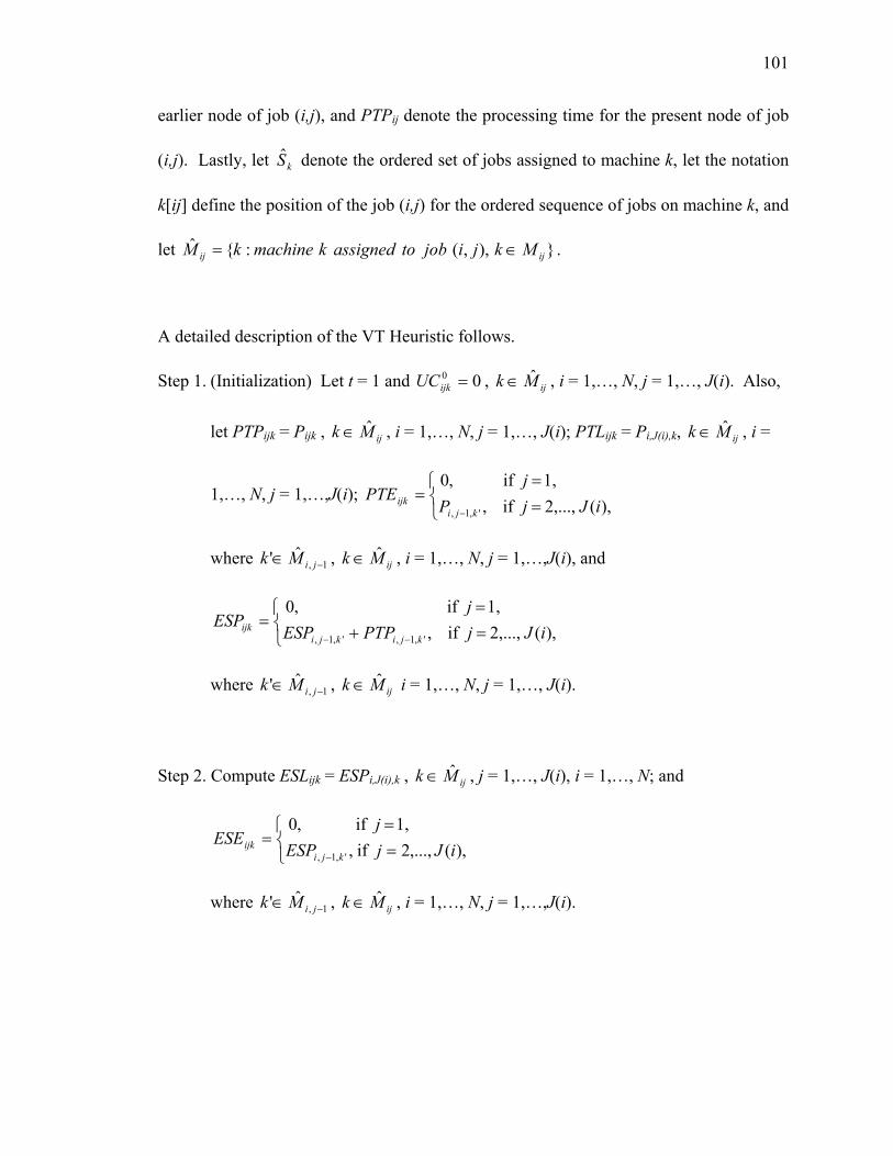
101
earlier node of job (i,j), and PTPij denote the processing time for the present node of job
(i,j). Lastly, let kS denote the ordered set of jobs assigned to machine k, let the notation
k[ij] define the position of the job (i,j) for the ordered sequence of jobs on machine k, and
let }),,(:{ˆijij MkjijobtoassignedkmachinekM ∈= .
A detailed description of the VT Heuristic follows.
Step 1. (Initialization) Let t = 1 and 00 =ijkUC , ijMk ˆ∈ , i = 1,…, N, j = 1,…, J(i). Also,
let PTPijk = Pijk , ijMk ˆ∈ , i = 1,…, N, j = 1,…, J(i); PTLijk = Pi,J(i),k, ijMk ˆ∈ , i =
1,…, N, j = 1,…,J(i); ⎩⎨⎧
==
=− ),( 2,..., if,
1, if,0
',1, iJjPj
PTEkji
ijk
where 1,ˆ' −∈ jiMk , ijMk ˆ∈ , i = 1,…, N, j = 1,…,J(i), and
⎩⎨⎧
=+=
=−− ),( 2,..., if,
1, if,0
',1,',1, iJjPTPESPj
ESPkjikji
ijk
where 1,ˆ' −∈ jiMk , ijMk ˆ∈ i = 1,…, N, j = 1,…, J(i).
Step 2. Compute ESLijk = ESPi,J(i),k , ijMk ˆ∈ , j = 1,…, J(i), i = 1,…, N; and
⎩⎨⎧
==
=− ),(,...,2 if,
1, if,0
',1, iJjESPj
ESEkji
ijk
where 1,ˆ' −∈ jiMk , ijMk ˆ∈ , i = 1,…, N, j = 1,…,J(i).

102
Step 3. Compute the urgency criterion ( tijkUC ) defined in Equations (4.1) – (4.3).
ijkijk
ijktijk PTPFPT
TWRUC
+= , ijMk ˆ∈ , i = 1,…, N, j = 1,…, J(i), (4.1)
where,
TWRijk = ESLijk + PTLijk - ESPijk, and (4.2)
FPTijk = ESEijk + PTEijk . (4.3)
Step 4. If tijkUC = 1−t
ijkUC , ijMk ˆ∈ , i = 1,…, N, j = 1,…, J(i), go to Step 6.
Otherwise, for each machine k, k = 1,…, M, arrange all jobs (i,j), such that
ijMk ˆ∈ , in kS in non-ascending order of the tijkUC values. Let t = t + 1.
Step 5. Recompute
⎪⎪⎩
⎪⎪⎨
⎧
>>++=>+>=+==
=
−−−−
−−
−−
,1][ and 1 if},,max{,1][ and 1 if,,1][ and 1 if,,1][ and 1 if,0
1][1][',1,',1,
',1,',1,
1][1][
ijkjPTPESPPTPESPijkjPTPESPijkjPTPESPijkj
ESP
ijkijkkjikji
kjikji
ijkijkijk
where 1,ˆ' −∈ jiMk , ijMk ˆ∈ , i = 1,…, N, j = 1,…,J(i),
and go to Step 2.
Step 6. Set =+= iPTLESLMS kiJikiJi :){(max ),(,),(, },...,1,,...,1 MkN = and stop.

103
End Start
1,1 M3
1,2 M1
1,3 M4
2,1 M2
2,2 M2
2,3 M4
3,1 M3
3,2 M1
3,3 M1
4,1 M4
4,2 M4
4,3 M1
5,1 M1
5,2 M1
5,3 M2
6,1 M3
6,2 M4
6,3 M1
Figure 4.5. Job Sequences at the End of the VT Heuristic
The job (i,j) with the maximum completion time is the critical job, and the time
associated with this job is the makespan MS. Henceforth, at the end of performing the
VT Heuristic, the makespan value yielded will be denoted as MSINIT (i.e., the initial
solution at the end of Stage I of the TS Algorithm). The sequence that contains this
critical job is known as the critical path (or the critical machine sequence - CMS), and
22
5
12
16 17
24
16
17
21
20
17
19
25
25
18
26
21
14
[0]
[82]
[60]
[114]
[135]
job, op m/c processing
time
Key: critical machine sequence (CMS) =
[ES] = earliest start time
[38]
[65]
[21] [98]
104
later designated as a seed sequence. In Figure 4.5, four job sequences that were
determined (from the results of the SPTR Heuristic example problem in Section 4.3.2)
after performing the VT Heuristic are shown. The critical machine sequence is denoted
as the path with the solid line and it has a final makespan MSINIT value of 149 time units.
This sequence is used as the seed sequence for the Stage II of the TS Algorithm.
4.5. Background on Generic Tabu Search Methodology
In Glover’s Tabu Search methodology, two important concepts – short-term memory
(STM) and long-term memory (LTM) – are employed. During the short-term memory
phase, the Tabu Search method intensifies the search for a solution by keeping limited
track of a few moves (i.e., job pairs that are kept on a Tabu list of a specified length) in
order to avoid cycling and guide the search out of a local optimum. At each iteration step
of the STM phase, a neighborhood of sequences is generated with the use of a
perturbation technique such as adjacent pairwise interchange (Baker, 2000; Croce, 1995;
French, 1982) from an initial seed sequence. Based on some objective function, the
neighborhood sequence that correlates to best solution is chosen as the seed sequence for
the next iteration, and the job pair that causes the perturbation of the initial seed sequence
is placed on a Tabu List (TL).
This TL (which is initially empty) is continuously updated (since it is cyclic) throughout
the search by adding and removing selected best moves (i.e., job pairs). In addition, this

105
list is updated circularly according to the TL size – that is, if the list was stored up to its
maximum size, the oldest (earliest at the top of list) move must be removed before adding
the next sequence. During subsequent iterations, before a neighborhood sequence is
chosen as having the best solution, the job pair in the sequence that causes the
perturbation of the seed is checked against the TL. If the job pair is present in the TL, the
move is marked as a forbidden move, and the next best solution value and neighborhood
sequence are inspected. Along the way, any improvements found in the overall objective
solution are stored and updated as well.
This is repeated for a period of time until some maximum number of STM iterations
(denoted later as Z and MAXSTM) since the initial iteration is reached. At this point, the
LTM phase is invoked. In this phase, performing some type of improvement procedure
such as moving jobs from one machine to another (as in the MOVE procedure described
in Section 4.3) to determine an improved solution for the objective function and allow the
search to diversify. This is considered as “re-starting” or “cleaning” the search, and it
uses previous STM searches to bias new searches. In addition, the LTM phase allows for
new unexplored regions to be searched, and old regions to be blocked from being visited
for some period of time. Next, the STM procedure is repeated by starting with a new
seed sequence that is determined from the best solution chosen during the prior LTM
phase. The entire methodology cycles repeatedly by switching between STM and LTM
phases until some maximum number of LTM iterations (denoted later as Z’ and
MAXNLTM) since the best improvement was last found or some pre-specified maximum

106
number of LTM iterations is attained. When this value is reached, the procedure stops,
and the best solution along with its associated sequences are revealed. A generic version
of Glover’s Tabu Search methodology is presented as follows.
Step 1. Retrieve some initial feasible sequence. Find its objective function value.
Step 2. Initialize the Tabu list as an empty set. Assign the initial solution as the best
solution.
Step 3. Do the following loop for some number of Z iterations during the STM phase.
Step 3a. Perturb the feasible sequence to get a new sequence.
Step 3b. Check to see if the new sequence is better than the best solution. If so,
assign the new sequence as the next seed sequence and place the move
associated with this new sequence on the TL while removing the
earliest move from the list.
Step 3c. If the best solution has improved, update the objective function value.
Step 4. Invoke the LTM phase and use the current best sequence as the new seed
sequence.
Step 4a. Create an evaluation criteria (or improvement procedure) that is
designed to produce a new starting point for the search. The criteria
should guide the heuristic process to regions in the search space that
contrast those explored thus far in order to try to improve on the best
solution.
107
Step 4b. If the evaluation criteria (or improvement procedure) provides a better
solution, assign the new sequence as the next seed sequence (Note: A
TL may or may not be used during this phase).
Step 4c. If the best solution has improved, update the objective function value.
Step 5. Repeat Step 3 and Step 4 until a number of Z’ iterations is reached during the
LTM phase or until no improvement in the objective function value has been
found for some number of Z’ iterations.
Step 6. Stop the heuristic once Z’ is reached. The best solution has been found along
with its associated sequences.
In this research, the Yijghk sequencing variables from the basic 0-1 MILP model previously
discussed in Chapter 3 are used in the STM phase of Stage II of the TS Algorithm to
intensify the search. When the seed sequence is perturbed during any given STM
iteration, the Yijghk sequencing variables are altered to reflect these changes. That is, jobs
are re-sequenced (reordered) such that the move may potentially improve the objective
value every time a new neighborhood sequence is formed.
The Xijk routing variables are used in the LTM phase of Stage II of the TS Algorithm to
diversify the search. Here, jobs are re-routed (re-allocated) such that moving a job from
one machine to another alters two or more sequences. This causes Xijk routing variables
to be altered and could potentially improve the objective value once more. Another
possibility for changing two or more sequences is by exchanging (i.e., switching) two

108
jobs on two different machines. In the scheduling research literature, usually one of these
procedures (moving jobs or switching jobs) is utilized; however, both are incorporated in
this research in an attempt to get improved results.
In summary, the intensification property of Glover’s Tabu Search meta-heuristic enables
the Yijghk sequencing variables to be extensively searched in a promising feasible region
of the solution space. This region is based on a given set of Xijk routing variables. When
no more improvements are found in this feasible region, the diversification property takes
over by allowing another unexplored feasible region to be searched using a new set of
sequences with modified Xijk variables. These two properties comprise the basic structure
of the TS Algorithm, and they are explained in greater detail in the next section.
4.6. Two-Stage Tabu Search Algorithm (TS Algorithm) Methodology
While there have been some use of Glover’s Tabu Search meta-heuristic method to solve
the FMS scheduling problem, the methodology presented in this research uses the Tabu
Search method in a new and unique way. The algorithm includes two stages: (1) a
method to generate initial feasible sequences of jobs is developed and used during the
construction stage, and (2) the Tabu Search meta-heuristic method is used in conjunction
with an efficient pairwise interchange (PI) method, LP sub-problem formulations, and job
reassignment procedures (i.e., MOVE and SWITCH procedures from Section 4.3), which
constitute the improvement stage. A snapshot of the TS Algorithm is shown in Figure

109
4.6. An overview of both Stage I and Stage II follows in the next sub-sections, and then
the detailed steps are given.
Figure 4.6. Snapshot of the TS Algorithm
Seed: 1-2-3-4 N1: 2-1-3-4 N2: 1-3-2-4
5
Improvement Phase – Stage II
Tabu Search – Short-term memory (TS-STM)
: :
Automatic generation of LP
Call LP solver for solution
LP Subroutine
Tabu List (STM) Iteration
2-1, 1-2 (Yijghk info.)
Iteration #2
Solution
8
Move/Switch Procedures – moves & switches jobs (Xijk information) then chooses best MS value & sequence
VT Heuristic – determines new job sequences & MS values
: :
Tabu Search – Long-term memory (TS-LTM)
Final STM Iteration
After no improvement in MS solution during a # of LTM iterations, STOP Heuristic and select final best makespan & sequences; Elsewise, proceed to TS-STM to perform STM iterations.
Return solution to TS STM
Choose best MS value (5) & proceed to Iteration #2 using N1 as new seed seq.
Iteration #1
After Final STM Iteration, proceed to Long-term memory (TS-LTM) with best MS and sequences
Retrieve Data
Construction Phase – Stage I
SPTr Heuristic -determines initial job routings
VT Heuristic – determines initial job sequences & initial makespan solution

110
4.6.1 Stage I of the TS Algorithm
The first stage of the algorithm utilizes two heuristics: (1) the SPTR Heuristic (from
Section 4.3) is used to initially allocate jobs to machines, and (2) the VT Heuristic (from
Section 4.4) is used to determine the initial feasible job sequences and an initial
makespan value. The combination of these two heuristics is denoted as the INIT
procedure from this point forward. Once the initial makespan value and job sequences
are determined, Stage II is invoked.
4.6.2 Stage II of the TS Algorithm
Next, the short-term memory (STM) function of the Tabu Search meta-heuristic
procedure is utilized. In this phase, neighborhood sequences are formed from the seed
sequence (i.e., the critical machine sequence) using the adjacent pairwise interchange
(API) method where two adjacent jobs are switched, and for each neighborhood sequence
(in conjunction with the other remaining sequences) an LP model is automatically
generated if the switch does not contain Tabu job pairs. This is equivalent to changing
the Yijghk sequencing variables in the original 0-1 MILP model previously described in
Chapter 3. Next, an LP solver (i.e., LP_Solve) subroutine is called to determine a MSLP
value for the current neighborhood sequence. This process is repeated for each
neighborhood sequence.

111
The 0-1 MILP model developed in Section 3.3 is the basis for the LP sub-problem used
within this heuristic methodology by fixing various Xijk and Yijghk variables. Recall from
Section 3.3.2 that the Xijk variables represent the routing determination factors (i.e., where
operations are assigned to machines) and the Yijghk variables represent the sequencing
determination factors (i.e., when the order to perform operations of jobs is determined).
When all of the Xijk and Yijghk variables are fixed in the basic MILP model, it becomes an
LP model that is solvable in polynomial time. This happens because once the Xijk and
Yijghk integer variables from the 0-1 MILP model are set to 0 and 1 values, the computer
no longer has to perform exhaustive enumeration using every possible combination of the
0 and 1 variables. At this point, the remaining variables no longer have integer
conditions. A job sequence is fixed, and optimal job starting times are easily obtainable
with the use of an optimization LP solver such as LP_Solve or Lingo. This entire
procedure of generating an LP model automatically, solving the LP model, and retrieving
a makespan solution value (MSLP) from the LP model is denoted as GENERATELP
henceforth.
A new subscript ijM (or ghM ), where },1:{ˆijijkij MkXkM ∈== is introduced, and it
represents the set of machines specifically assigned to process job (i,j). The transformed
version of the original 0-1 MILP model (from Section 3.4) into the new LP model is
shown in the following mathematical formulation:
Min MS (4.4)

112
s.t.
,1, +≤+ jiijkij BPB i = 1, 2, …, N; j = 1, 2, …, J(i)-1; ijMk ˆ∈ . (4.5)
,0)()(, ≤−+ MSPB kiiJiJi i = 1, 2, …, N; )(ˆ
iiJMk ∈ . (4.6)
,0≥−− ghkghij PBB (4.7)
i = 1, 2, …, N; g = 1, 2, …, N; i ≠ g; j = 1, 2, …, J(i);
h = 1, 2, …, J(g); ghij MMk ˆˆ ∩∈ and Yijghk = 0.
,0≥−− ijkijgh PBB (4.8)
i = 1, 2, …, N; g = 1, 2, …, N; i ≠ g; j = 1, 2, …, J(i);
h = 1, 2, …, J(g); ghij MMk ˆˆ ∩∈ and Yijghk = 1.
,1 ii RB ≥ i = 1, 2, …, N. (4.9)
,0≥ijB i = 1, 2, …, N; j = 2, …, J(i). (4.10)
,0≥MS (4.11)
Notations are defined in Section 3.3, and the constraint set definitions are similar to those
described previously in Section 3.4. In a makespan scheduling problem, this formulation
113
becomes useful for finding optimal starting and completion times quickly. Additionally,
with an E/T scheduling problem, this becomes useful for identifying optimal inserted idle
times. Thus, instead of creating a heuristic methodology that has no optimality in its
structure, using newly generated LP models within Tabu Search guarantee some degree
of optimality during each iteration of the methodology. In order to optimally solve the
LP subproblems at each iteration, a free MILP/LP solver called LP_Solve is integrated
and used within the C++ coded TS Algorithm.
From all solution sequences determined, the best sequence is chosen and becomes the
next seed sequence during the following iteration. It should be noted that the best
solution might not necessarily be the one that improves the overall solution, but it helps
the procedure to escape from being trapped at a local optima. In addition, the pair of jobs
that were interchanged (according to the original seed sequence) is added to the short-
term Tabu list (TL). This cyclic list is used to keep track of a few moves where the
search was previously performed, and it is constantly updated during each STM iteration.
Any pair of jobs that is on the TL during later iterations is forbidden to be used to
generate a new sequence. This mechanism helps to avoid cycling and getting the same
seed sequence and neighborhood sequences during subsequent iterations. The entire
process is repeated for some maximum number of short-term iterations (MAXSTM) before
the LTM function is invoked. However, at some point in time, every move in a
neighborhood may contain a Tabu move. If this happens, another function of the Tabu

114
Search meta-heuristic is activated. This function is known as aspiration A, and its
purpose is to restrict the search from being trapped at a solution surrounded by Tabu
neighbors. When a neighborhood has only Tabu solutions, the sequence with the
smallest solution that is greater than the aspiration value is chosen as the next candidate
seed sequence.
If at any time during the STM phase the makespan for the TS Algorithm (MSTS) is
improved, the makespan value found during the STM iteration (MSSTM) is updated as the
current best makespan (i.e., MSTS = MSSTM). Also, the sequence associated with this MSTS
value becomes the current best seed sequence, and the aspiration value is updated A =
MSSTM. This information is carried into the next step of the algorithm – the LTM phase
of the Tabu Search.
In the LTM phase, the idea is to bias the search such that a new search space is explored
in order to try to improve the objective. In this research, two features are investigated.
The first feature uses a procedure named MOVE (Step 4 of the SPTR Heuristic from
Section 4.3) in which jobs in the seed sequence are shifted (i.e., moved) from their
current machines to different machines if job alternatives exist for any particular
operation. The determination of the makespan value during this step is not necessary; so,
it is ignored for now. From this point, the VT Heuristic is called upon to rearrange the
job sequences into the best order that may yield the best possible makespan value based
on the change. Hence, the Yijghk sequencing variables are changed while using a modified
115
set of Xijk routing variables (i.e., routing variables). The second feature uses a procedure
named SWITCH (Step 5 of the SPTR Heuristic from Section 4.3). Wherein, jobs on the
bottleneck machine, which contains the seed sequence, are interchanged (i.e., switched)
with other jobs in one of the other machines if job alternatives exist, and the makespan
determination is ignored once more at this step. Then, the VT Heuristic is utilized again
to determine the makespan value after the switch of jobs is performed.
Both the MOVE and SWITCH procedures are equivalent to changing the Xijk routing
variables in the original 0-1 MILP model previously described in Chapter 3. This is a
new approach to solving the FMC scheduling problem, since most of the literature
usually focus on just changing the job sequences (Y variables) or the job routes (X
variables) but usually not both simultaneously within the same methodology. After
finding the best makespan solution from either the MOVE or SWITCH procedures,
denoted as MSLTM, the critical machine sequence associated with this makespan solution
is used as the new seed sequence, and the short-term memory phase is repeated once
more. From here, both STM and LTM phases are repeated until there is no improvement
in the overall makespan value for a number of long-term memory iterations (MAXNLTM).
Once this value is reached, the algorithm stops.
Next, a detailed description of the TS Algorithm is presented. Let SIZETL denote the size
of the TL, ISTM denote the STM iteration counter, ILTM denote the LTM iteration counter,
and INLTM denote a counter which represents that no improvement was found for the MSTS

116
value at the end of a LTM iteration. Let MSMOVE denote the best makespan solution
found during the MOVE procedure, and MSSWITCH denote the best makespan solution
found during the SWITCH procedure. Recall from Section 3.3.2 that γ is a large positive
integer value used in the disjunctive constraints, but here it to reset certain MS values.
4.6.3 Detailed Description of the TS Algorithm
Stage I (Data retrieval and perform initial heuristics)
Step 1: Retrieve scheduling data. This includes all job processing times, all job
sequences, and all machines that are available for each job.
Step 2: Invoke the INIT procedure to get an initial makespan value (MSINIT) and its
associated seed sequence.
Stage II (STM & LTM phases)
Step 3. Initialize parameters
Let MAXSTM = 8; MAXNLTM = 5; SIZETL = 4 (these values are determined in
Chapter 5); TL = ∅; ISTM = 0; ILTM = 0; INLTM = 0; MSSTM = γ; MSLTM = γ; MSLP =
γ; A = MSINIT; MSMOVE = γ; MSSWITCH = γ; and MSTS = MSINIT.
Step 4. Invoke the Tabu Search – Short Term Memory (STM) Phase

117
(1) Form neighborhood sequences from the seed sequence using API by
interchanging adjacent jobs in each sequence if the job moves are not tabu.
If all job moves are tabu (i.e., forbidden interchanged job pairs that are
already on set TL), aspiration occurs. During aspiration, for each tabu
neighborhood sequence perform the GENERATELP procedure to determine a
MSLP. Select the sequence with the smallest MSLP value, such that MSLP > A,
as the next seed sequence and go to Step 4-3. If all job moves are not tabu,
perform the GENERATELP procedure to determine a MSLP for each feasible
non-tabu neighborhood sequence.
(2) Examine each neighborhood sequence to choose the best neighborhood
solution as the next seed sequence. Let LPSM ˆ be the MS value for the best
neighborhood sequence. If LPSM ˆ < MSSTM, then let MSSTM = LPSM ˆ and A =
MSSTM. Assign the sequence associated with the solution that corresponds to
the best MSSTM as the next seed sequence and update the set TL. If MSSTM <
MSTS, let MSTS = MSSTM, assign its associated sequence as the overall best
sequence and go to Step 4-3.
(3) Let ISTM = ISTM + 1. If ISTM = MAXSTM, then let ISTM = 0, MSSTM = γ, A = γ,
and go to Step 5.
Otherwise, let MSSTM = γ and repeat Step 4.
Step 5. Invoke the Tabu Search – Long Term Memory (LTM) Phase
(1) Generate a new seed sequence from the current seed sequence by moving one
job to another machine using the MOVE procedure:
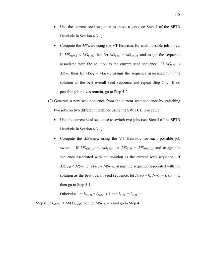
118
• Use the current seed sequence to move a job (see Step 4 of the SPTR
Heuristic in Section 4.3.1).
• Compute the MSMOVE using the VT Heuristic for each possible job move.
If MSMOVE < MSLTM, then let MSLTM = MSMOVE and assign the sequence
associated with the solution as the current seed sequence. If MSLTM <
MSTS, then let MSTS = MSLTM, assign the sequence associated with the
solution as the best overall seed sequence and repeat Step 5-1. If no
possible job moves remain, go to Step 5-2.
(2) Generate a new seed sequence from the current seed sequence by switching
two jobs on two different machines using the SWITCH procedure:
• Use the current seed sequence to switch two jobs (see Step 5 of the SPTR
Heuristic in Section 4.3.1)
• Compute the MSSWITCH using the VT Heuristic for each possible job
switch. If MSSWITCH < MSLTM, let MSLTM = MSSWITCH and assign the
sequence associated with the solution as the current seed sequence. If
MSLTM < MSTS, let MSTS = MSLTM, assign the sequence associated with the
solution as the best overall seed sequence, let INLTM = 0, ILTM = ILTM + 1,
then go to Step 5-1.
Otherwise, let INLTM = INLTM + 1 and ILTM = ILTM + 1.
Step 6. If INLTM < MAXNLTM, then let MSLTM = γ and go to Step 4.

119
Otherwise, STOP the TS Algorithm. The best makespan value (MSTS) has been
found along with its associated machine sequences. At this time, a production
schedule can be generated.
4.6.4 Illustrative Example of the TS Algorithm
Suppose that Stage I (i.e., the INIT procedure) was previously performed (as detailed in
Section 4.3 and Section 4.4), resulting with an initial makespan solution of 122 (MSINIT),
and seed sequence on machine 1 (see Figure 4.4). From this point, Stage I (i.e., Steps 1 –
2) is completed and Stage II of this example problem is outlined next.
Step 3. Initialize parameters
Let MAXSTM = 8; MAXNLTM = 5; SIZETL = 4; (for this example only)
TL = {∅}; ISTM = 0; ILTM = 0; INLTM = 0; MSSTM = γ; MSLTM = γ; MSLP = γ ; A =
149; MSMOVE = γ; MSSWITCH = γ; and MSTS = 149. (Note: γ is a very large number)
Step 4. Invoke the Tabu Search – Short Term Memory (STM) Phase
The information in Table 4.5, Table 4.6 and Table 4.7 show a summary of Step 4 of the
TS Algorithm. Each column represents the STM iteration counter, neighborhood
sequence number, the actual neighborhood sequence, the makespan solution value, and
the actual Tabu list. Each table is explained in greater detail in the following paragraphs.
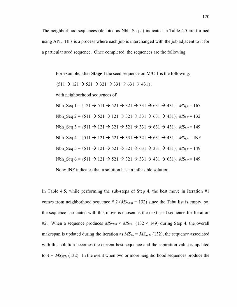
120
The neighborhood sequences (denoted as Nbh_Seq #) indicated in Table 4.5 are formed
using API. This is a process where each job is interchanged with the job adjacent to it for
a particular seed sequence. Once completed, the sequences are the following:
For example, after Stage I the seed sequence on M/C 1 is the following:
{511 121 521 321 331 631 431},
with neighborhood sequences of:
Nbh_Seq 1 = {121 511 521 321 331 631 431}; MSLP = 167
Nbh_Seq 2 = {511 521 121 321 331 631 431}; MSLP = 132
Nbh_Seq 3 = {511 121 321 521 331 631 431}; MSLP = 149
Nbh_Seq 4 = {511 121 521 331 321 631 431}; MSLP = INF
Nbh_Seq 5 = {511 121 521 321 631 331 431}; MSLP = 149
Nbh_Seq 6 = {511 121 521 321 331 431 631}; MSLP = 149
Note: INF indicates that a solution has an infeasible solution.
In Table 4.5, while performing the sub-steps of Step 4, the best move in Iteration #1
comes from neighborhood sequence # 2 (MSSTM = 132) since the Tabu list is empty; so,
the sequence associated with this move is chosen as the next seed sequence for Iteration
#2. When a sequence produces MSSTM < MSTS (132 < 149) during Step 4, the overall
makespan is updated during the iteration as MSTS = MSSTM (132), the sequence associated
with this solution becomes the current best sequence and the aspiration value is updated
to A = MSSTM (132). In the event when two or more neighborhood sequences produce the
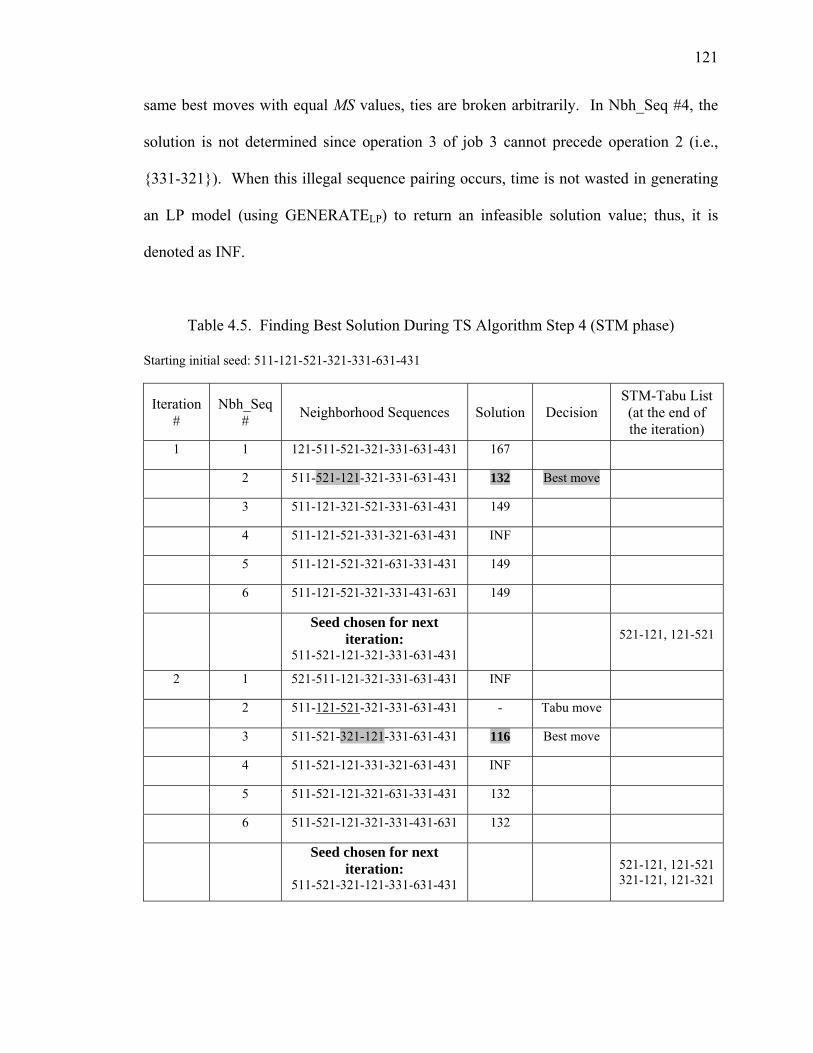
121
same best moves with equal MS values, ties are broken arbitrarily. In Nbh_Seq #4, the
solution is not determined since operation 3 of job 3 cannot precede operation 2 (i.e.,
{331-321}). When this illegal sequence pairing occurs, time is not wasted in generating
an LP model (using GENERATELP) to return an infeasible solution value; thus, it is
denoted as INF.
Table 4.5. Finding Best Solution During TS Algorithm Step 4 (STM phase)
Starting initial seed: 511-121-521-321-331-631-431
Iteration #
Nbh_Seq # Neighborhood Sequences Solution Decision
STM-Tabu List (at the end of the iteration)
1 1 121-511-521-321-331-631-431 167
2 511-521-121-321-331-631-431 132 Best move
3 511-121-321-521-331-631-431 149
4 511-121-521-331-321-631-431 INF
5 511-121-521-321-631-331-431 149
6 511-121-521-321-331-431-631 149
Seed chosen for next
iteration: 511-521-121-321-331-631-431
521-121, 121-521
2 1 521-511-121-321-331-631-431 INF
2 511-121-521-321-331-631-431 - Tabu move
3 511-521-321-121-331-631-431 116 Best move
4 511-521-121-331-321-631-431 INF
5 511-521-121-321-631-331-431 132
6 511-521-121-321-331-431-631 132
Seed chosen for next
iteration: 511-521-321-121-331-631-431
521-121, 121-521 321-121, 121-321

122
In addition, the sequence job pairs {521-121, 121-521} are added to the TL, and MSSTM
and A were updated as 132. In Iteration #2, the API switch of jobs during Nbh_Seq #2
produces an illegal pairing of {121-521}. Since this pair of jobs is already on the TL, the
sequence is bypassed and the LP model is not generated. The sequence in Nbh_Seq #3
produces the best move and its solution of 116 improves the overall solution as well,
thus, MSSTM, MSTS, and A are updated as 116. In addition, its associated sequence
becomes the current best sequence, and the TL is updated again with a second set of
sequence job pairs {321-121, 121-321}.
The continuation of the TS Algorithm is presented in Table 4.6. In Iteration #3, another
sequence is determined as infeasible (Nbh_Seq #1), and the sequence in Nbh_Seq #3 has
a Tabu move. Thus, both are bypassed and not used. The sequence in Nbh_Seq #4
produces the best move and its solution of 115 improves the overall solution once again.
Therefore, MSSTM, MSTS, and A are updated as 115, and the TL is updated once more with
a third set of sequence job pairs {331-121, 121-331}. In Iteration #4, two sequences are
found as infeasible (Nbh_Seq #1 and Nbh_Seq #3), and one sequence has a Tabu move
(Nbh_Seq #3), so these sequences are all bypassed and not used. The overall sequence is
not improved in this iteration.
The remaining iterations of this example are summarized in Table 4.7. For Iteration #5
through Iteration #7, only the best sequences and solutions chosen are displayed along
with the updated Tabu list. In the final Iteration #8 in Table 4.7, all neighborhood

123
sequence information is presented. Additionally, the final MSSTM yields a value of 115
(which is also equivalent to overall best solution MSTS). Since ISTM = 8 (MAXSTM), the
values for MSSTM and A are reset just before Step 4 ends, and the algorithm progresses to
Step 5.
Table 4.6. Continuation of the TS Algorithm Step 4 (STM phase)
Iteration #
Nbh_Seq # Neighborhood Sequences Solution Decision
STM-Tabu List (at the end of the iteration)
3 1 521-511-321-121-331-631-431 INF
2 511-321-521-121-331-631-431 127
3 511-521-121-321-331-631-431 - Tabu move
4 511-521-321-331-121-631-431 115 Best move
5 511-521-321-121-631-331-431 116
6 511-521-321-121-331-431-631 116
Seed chosen for next
iteration: 511-521-321-331-121-631-431
521-121, 121-521 321-121, 121-321 331-121, 121-331
4 1 521-511-321-331-121-631-431 INF
2 511-321-521-331-121-631-431 127
3 511-521-331-321-121-631-431 INF
4 511-521-321-121-331-631-431 - Tabu move
5 511-521-321-331-631-121-431 122
6 511-521-321-331-121-431-631 115 Best move
Seed chosen for next
iteration: 511-521-321-331-121-431-631
521-121, 121-521 321-121, 121-321 331-121, 121-331 431-631, 631-431

124
Table 4.7. Summary of Remaining Iterations of TS Algorithm Step 4 (STM phase)
Iteration #
Nbh_Seq # Neighborhood Sequences Solution Decision
STM-Tabu List (at the end of the iteration)
5 5 (chosen) Seed chosen for next
iteration: 511-521-321-331-431-121-631
115 Best move 321-121, 121-321 331-121, 121-331 431-631, 631-431 431-121, 121-431
6 4 (chosen) Seed chosen for next
iteration: 511-521-321-431-331-121-631
115 Best move 331-121, 121-331 431-631, 631-431 431-121, 121-431 431-331, 331-431
7 3 (chosen) Seed chosen for next
iteration: 511-521-431-321-331-121-631
116 Best move 431-631, 631-431 431-121, 121-431 431-331, 331-431 431-321, 321-431
8 1 521-511-431-321-331-121-631 INF
2 511-431-521-321-331-121-631 133
3 511-521-321-431-331-121-631 - Tabu move
4 511-521-431-331-321-121-631 INF
5 511-521-431-321-121-331-631 115 Best move
6 511-521-431-321-331-631-121 137
Seed chosen for next
iteration: 511-521-431-321-121-331-631
431-121, 121-431 431-331, 331-431 431-321, 321-431 121-331, 331-121
Next, all job sequence information is carried into Step 5 of the TS Algorithm – the LTM
phase of TS Algorithm. The current job sequences are shown in Figure 4.7, with the
critical machine sequence on machine 1.

125
Figure 4.7. Job Sequences at the End of the TS Algorithm Step 4 (STM phase)
Step 5. Invoke the Tabu Search – Long Term Memory (LTM) Phase
(1) Evaluate the current seed sequence using the MOVE procedure:
• Use the seed sequence to move a job (see Step 4 of the SPTR Heuristic in
Section 4.3.1)
The job (5,2) and machines (1,2) are identified: i = 5, j = 2, k = 1, k’ = 2.
S1 = S1 \{(5,2)} = {(5,1), (3,2), (3,3), (1,2), (6,3), (4,3)};
S2 = )}2,5{(2 ∪S = {(2,1), (2,2), (5,3), (5,2)}.
The shifting action of moving a job from one machine to another is depicted
in Figure 4.8.
M/C 1 sequence = {511 521 321 331 121 631 431}
M/C 2 sequence = {212 222 532}
M/C 3 sequence = {613 313 113}
M/C 4 sequence = {414 424 624 234 134}
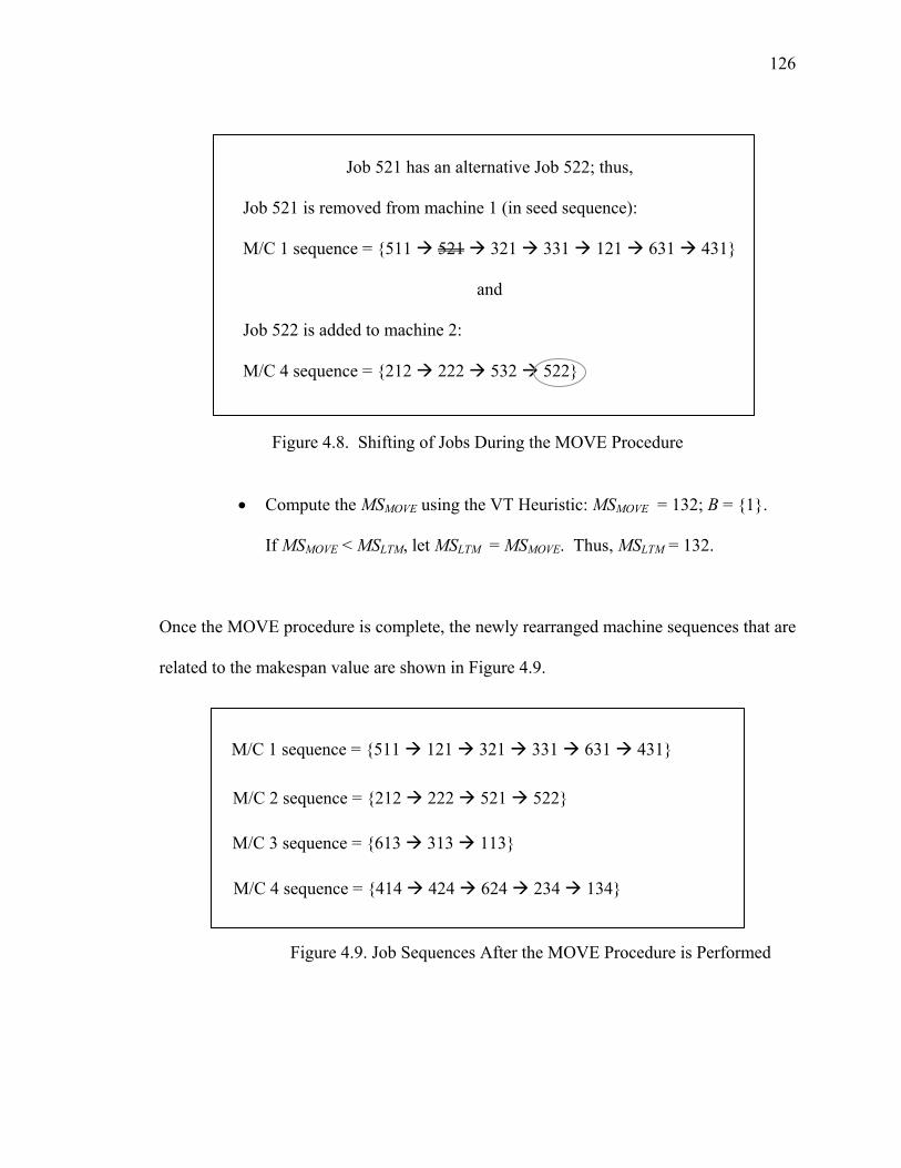
126
Job 521 has an alternative Job 522; thus, Job 521 is removed from machine 1 (in seed sequence): M/C 1 sequence = {511 521 321 331 121 631 431}
and
Job 522 is added to machine 2: M/C 4 sequence = {212 222 532 522}
Figure 4.8. Shifting of Jobs During the MOVE Procedure
• Compute the MSMOVE using the VT Heuristic: MSMOVE = 132; B = {1}.
If MSMOVE < MSLTM, let MSLTM = MSMOVE. Thus, MSLTM = 132.
Once the MOVE procedure is complete, the newly rearranged machine sequences that are
related to the makespan value are shown in Figure 4.9.
Figure 4.9. Job Sequences After the MOVE Procedure is Performed
M/C 1 sequence = {511 121 321 331 631 431}
M/C 2 sequence = {212 222 521 522}
M/C 3 sequence = {613 313 113}
M/C 4 sequence = {414 424 624 234 134}

127
Repeat Step 5-1 for remaining jobs in the current seed sequence if possible.
The job (3,3) and machines (1,2) are identified: i = 3, j = 3, k = 1, k’ = 2.
S1 = S1 \{(3,3)} = {(5,1), (5,2), (3,2), (1,2), (6,3), (4,3)};
S2 = )}3,3{(2 ∪S = {(2,1), (2,2), (5,3), (3,3)}.
After the jobs are shifted, MSMOVE is computed using the VT Heuristic:
MSMOVE = 117; B = {1}.
If MSMOVE < MSLTM, let MSLTM = MSMOVE. Thus, MSLTM = 117.
Since the remaining jobs in the current seed sequence do not have alternative jobs
available, the algorithm proceeds to the SWITCH procedure.
(2) Evaluate the current seed sequence using the SWITCH procedure:
• Use the seed sequence to switch two jobs (see Step 5 of the SPTR
Heuristic in Section 4.3.1)
The jobs (5,2), (2,1) and machines (1,2) are identified:
i = 5, j = 2, i’ = 2, j’ = 1, k = 1, k’ = 2.
S1 = [S1 \{(5,2)}] ∪ {(2,1)} = {(5,1), (2,1), (3,2), (3,3), (1,2), (6,3), (4,3)};
S2 = [S2 \{(2,1)}] ∪ {(5,2)} = {(5,2), (2,2), (5,3)}.
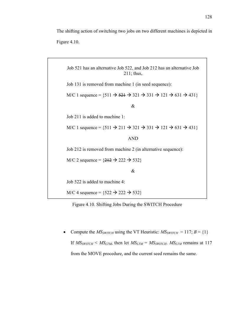
128
The shifting action of switching two jobs on two different machines is depicted in
Figure 4.10.
Figure 4.10. Shifting Jobs During the SWITCH Procedure
• Compute the MSSWITCH using the VT Heuristic: MSSWITCH = 117; B = {1}
If MSSWITCH < MSLTM, then let MSLTM = MSSWITCH. MSLTM remains at 117
from the MOVE procedure, and the current seed remains the same.
Job 521 has an alternative Job 522, and Job 212 has an alternative Job 211; thus,
Job 131 is removed from machine 1 (in seed sequence): M/C 1 sequence = {511 521 321 331 121 631 431}
&
Job 211 is added to machine 1: M/C 1 sequence = {511 211 321 331 121 631 431}
AND Job 212 is removed from machine 2 (in alternative sequence): M/C 2 sequence = {212 222 532}
& Job 522 is added to machine 4: M/C 4 sequence = {522 222 532}
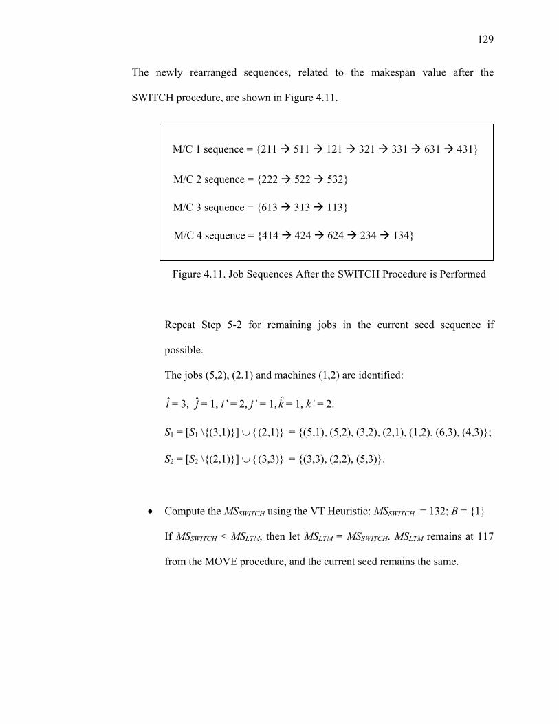
129
The newly rearranged sequences, related to the makespan value after the
SWITCH procedure, are shown in Figure 4.11.
Figure 4.11. Job Sequences After the SWITCH Procedure is Performed
Repeat Step 5-2 for remaining jobs in the current seed sequence if
possible.
The jobs (5,2), (2,1) and machines (1,2) are identified:
i = 3, j = 1, i’ = 2, j’ = 1, k = 1, k’ = 2.
S1 = [S1 \{(3,1)}] ∪ {(2,1)} = {(5,1), (5,2), (3,2), (2,1), (1,2), (6,3), (4,3)};
S2 = [S2 \{(2,1)}] ∪ {(3,3)} = {(3,3), (2,2), (5,3)}.
• Compute the MSSWITCH using the VT Heuristic: MSSWITCH = 132; B = {1}
If MSSWITCH < MSLTM, then let MSLTM = MSSWITCH. MSLTM remains at 117
from the MOVE procedure, and the current seed remains the same.
M/C 1 sequence = {211 511 121 321 331 631 431}
M/C 2 sequence = {222 522 532}
M/C 3 sequence = {613 313 113}
M/C 4 sequence = {414 424 624 234 134}
130
There are no more jobs in the current seed sequence with job alternatives that can be
switched; thus, the algorithm proceeds to Step 4 with the best minimum solution from the
LTM phase (which occurred in the MOVE procedure). The current seed sequence
associated with this value is the new seed sequence for the STM phase.
MSLTM = 117.
Since the MOVE procedure has the best LTM solution, the sequence of jobs on machine
1 becomes the new seed sequence: S1 = {(5,1), (3,2), (1,2), (5,2), (6,3), (4,3)}. All of the
job sequences associated with this move are now used for the next round of STM
iterations. INLTM and ILTM are updated to 1. MSTS was not improved during this LTM
phase.
Step 6. Since INLTM < MAXNLTM, reset MSLTM = γ and go to Step 4.
During a latter STM iteration after the LTM has been performed twice, the overall MSTS
was improved to 108. Next, the overall makespan never improved and algorithm
continued until INLTM = 5 (i.e., the MAXNLTM). Once that value was reached, the algorithm
stopped and the best overall makespan remained at 108. In addition, this solution
happens to be equivalent to the optimal solution found using the 0-1 MILP model from
Chapter 3.

131
4.7. Concluding Summary
In summary, several contributions have been presented in this chapter. First, the SPTR
Heuristic was developed to solve the routing sub-problem in Stage I of the overall TS
Algorithm. The effectiveness of this heuristic was shown in a comparison test with an
existing routing heuristic – the ECT Heuristic. When the SPTR Heuristic was combined
with the pre-existing VT Heuristic, the two heuristics jointly formed the INIT procedure.
Here, the sequencing sub-problem in Stage I of the overall TS Algorithm was solved, and
an initial makespan solution was determined. In Stage II of the TS Algorithm, Glover’s
Tabu Search meta-heuristic method was utilized. In the STM phase, the API method and
the automatic generation of LP model formulations were combined to re-sequence jobs,
while MOVE and SWITCH procedures were borrowed from the SPTR Heuristic and
utilized in the LTM phase to re-route jobs in order to find improved solutions. With all
of these methodologies combined, the TS Algorithm was determined to be a very useful
algorithm for solving FMC scheduling problems.
Finding the optimal (or near-optimal) makespan value is crucial for many situations in
the real world, however, the major improvement comes in how fast the TS Algorithm
solves the FMC problem. It only took 14.511 seconds to solve the example problem
optimally versus 8.01 hours using the 0-1 MILP model. The CPU time-savings is
significant when using the TS algorithm; thus, this heuristic methodology is very useful
in solving larger FMC scheduling problems which could take days or weeks to find an

132
optimal solution when using the traditional 0-1 MILP model approach. In Chapter 5,
computational results show that this approach is indeed faster than using full 0-1 MILP
approach, and that it provides optimal or near-optimal solutions for various size FMC
scheduling problems.

133
Chapter 5
COMPUTATIONAL RESULTS
5.1. Introduction
In an effort to evaluate the performance of the developed solution methodology in
Chapter 4, the TS Algorithm was tested and compared with the full 0-1 MILP model, the
2-MILP model, and the INIT procedure. Two tests were performed: (1) a preliminary
test to determine which Tabu parameters were to be selected and used during the main
test, and (2) a main test with full computational results which compares the various
methods by observing the average makespan values and average CPU runtime values for
small, medium, and large size FMC problems. In addition, the average relative error
(RE) from the optimal solutions (found using the 0-1 MILP model) for small-size FMC
problems, and the average RE from a lower bound (LB) for medium and large-size FMC
problems.
5.2. Preliminary Test
The MILP formulations, LP formulations, and TS Algorithm described in Chapter 3 and
Chapter 4 have been coded in Microsoft Visual C++ .NET and run on a Pentium 4
2.0GHz PC. Since no sample problems have been found in the literature that could be
used as a benchmark for testing the TS Algorithm, all of the processing times and
machine routing alternatives (similar to those found in Table 4.1) have been randomly
generated for all test problems, and the associated parameters used are displayed in Table

134
5.1. The number of jobs, number of operations, and number of machines determines the
size of each test problem. The number of jobs ranges between 3 and 10, while the
number of operations vary between 2 or 3 and the number of machines is either 3 or 4.
Job processing times have been generated using an integer uniform distribution as shown
in Table 5.1.
Table 5.1. Parameters Used for Small, Medium, and Large-size Preliminary Test Problems
DATA TEST VALUES Number of jobs (NJ) 3, 5, 10
Number of operations (NO) 2, 3 Number of machines (NM) 3, 4
Max. number of STM iterations (MAXSTM) 8, 14, 20 Max. number of LTM non-improvement
iterations (MAXNLTM) 5, 10
Tabu List size (SIZETL) 4, 7 Processing times (PT) Uniform [5,30]
Other parameters such as the number of short-term memory iterations (MAXSTM),
maximum number of long-term memory iterations (MAXNLTM) while no improvement in
solution value is found, and Tabu list size (SIZETL) are given as well. All MILP and LP
formulations (including those which are automatically generated in the TS Algorithm),
have been solved using the LP_Solve 5.5 MILP Solver to find optimal solutions
whenever possible.
The experiments are divided into two parts: a preliminary test and a main test (in Section
5.3). In the preliminary test, 12 test problems of various sizes (144 cases in total) were

135
generated according to the data in Table 5.1. These problems were solved for the FMC
scheduling problem to investigate the best combination of parameters to use in the main
test for the TS Algorithm. The computational results of the preliminary test for
makespan values are shown in Table 5.2.
For all of the test problems in the preliminary test, the makespan values found for each of
the given parameters were equivalent. Thus, from observation, any combination of
parameters could be selected. However, in order to justify the best combination of
parameters selected, the total CPU time was observed as well for each problem. The
results of the preliminary test for total CPU time are shown in Table 5.3. Observing the
computational results, the smallest average total CPU time for each combination of
parameters resulted in 30.495 seconds. This correlates to the following parameter
settings: (a) MAXSTM = 8, (b) MAXNLTM = 5, and (c) SIZETL = 7, which are the
parameter values that are chosen for the forthcoming main test problems based on the
preliminary test results. The most significant difference was observed when using the
various values (e.g., 8, 14, 20) for the number of short-term memory iterations. For each
MAXSTM parameter, selecting the value of 5 for the MAXNLTM parameter yielded the
shortest CPU times for every case as compared to the value of 10 for MAXNLTM, thus, the
value of 10 is value should not be used. The SIZETL parameter values (e.g., 4, 7) did not
show much significance in combination with the other parameters; thus, the size of the
TL could be selected as either 4 or 7. As noted above, the SIZETL parameter was set to 7
in this study.
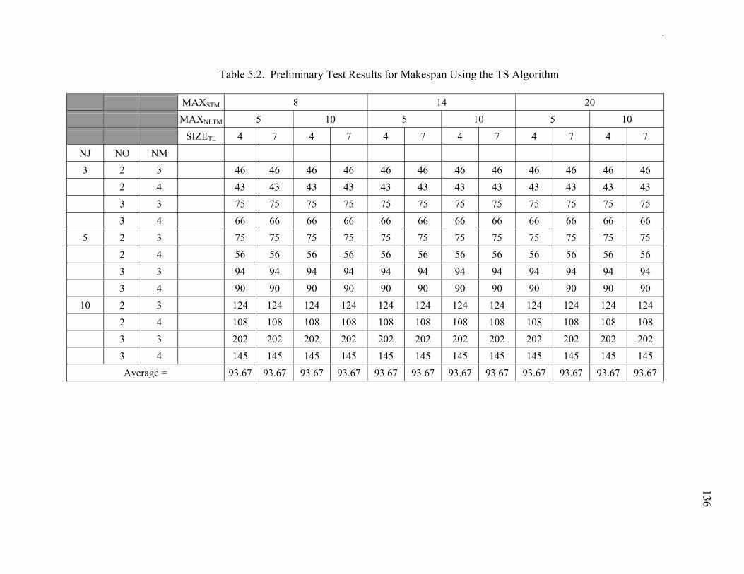
136
Table 5.2. Preliminary Test Results for Makespan Using the TS Algorithm
MAXSTM 8 14 20 MAXNLTM 5 10 5 10 5 10 SIZETL 4 7 4 7 4 7 4 7 4 7 4 7
NJ NO NM 3 2 3 46 46 46 46 46 46 46 46 46 46 46 46 2 4 43 43 43 43 43 43 43 43 43 43 43 43 3 3 75 75 75 75 75 75 75 75 75 75 75 75 3 4 66 66 66 66 66 66 66 66 66 66 66 66
5 2 3 75 75 75 75 75 75 75 75 75 75 75 75 2 4 56 56 56 56 56 56 56 56 56 56 56 56 3 3 94 94 94 94 94 94 94 94 94 94 94 94 3 4 90 90 90 90 90 90 90 90 90 90 90 90
10 2 3 124 124 124 124 124 124 124 124 124 124 124 124 2 4 108 108 108 108 108 108 108 108 108 108 108 108 3 3 202 202 202 202 202 202 202 202 202 202 202 202 3 4 145 145 145 145 145 145 145 145 145 145 145 145
Average = 93.67 93.67 93.67 93.67 93.67 93.67 93.67 93.67 93.67 93.67 93.67 93.67
. 136

137
Table 5.3. Preliminary Test Results for Total CPU Time (sec) Using the TS Algorithm
MAXSTM 8 14 20 MAXNLTM 5 10 5 10 5 10 SIZETL 4 7 4 7 4 7 4 7 4 7 4 7
NJ NO NM 3 2 3 2.614 2.704 4.837 4.967 3.558 4.847 7.721 8.422 6.320 6.810 11.597 11.777
2 4 1.532 1.693 2.633 2.954 2.764 3.054 4.897 5.048 3.505 4.056 6.600 7.000
3 3 6.049 6.549 10.706 11.241 10.835 11.177 16.703 18.727 15.442 16.569 24.475 24.590
3 4 3.485 3.626 6.179 6.299 6.249 7.215 10.475 10.736 8.812 8.933 14.301 14.341
5 2 3 8.462 8.663 16.253 15.091 14.991 14.561 26.979 27.272 22.976 21.011 38.075 35.561
2 4 5.088 5.357 10.205 9.684 9.296 9.834 17.178 18.126 12.898 13.419 25.317 24.495
3 3 21.351 20.800 35.921 34.279 36.712 38.145 59.185 58.915 53.117 51.794 84.261 84.491
3 4 16.113 16.293 28.781 28.434 28.951 28.291 50.373 52.071 38.015 39.046 68.419 69.009
10 2 3 57.492 56.453 99.012 98.671 99.383 99.693 177.615 173.890 144.508 143.276 249.589 244.011
2 4 31.242 31.124 55.530 57.182 50.853 50.943 92.810 93.445 72.605 74.437 131.940 135.004
3 3 136.777 135.974 249.208 247.456 237.962 234.417 439.081 424.281 341.270 333.590 623.066 611.897
3 4 77.231 76.700 142.374 139.651 139.250 140.651 254.422 259.341 197.357 208.791 363.483 374.939
Average = 30.620 30.495 55.137 54.659 53.400 53.569 96.453 95.856 76.402 76.811 136.760 136.426
137.

138
5.3. 0-1 MILP Model Characterization
Before analyzing the TS Algorithm, the computational requirements of the 0-1 MILP
formulations were observed in an example problem using 3 different runs. Table 5.4
shows Run #1 with 6 test problems that were randomly generated for a 4-machine 3-
operation problem using a number of jobs ranging from 2 to 7. The processing times
were generated in a similar fashion as those in Table 4.1 from Section 4.2.2. For each
test case (i.e., data set) problem, the table shows the following information: number of
jobs, operations, and machines evaluated; number of variables, integer variables, and
constraints generated; best makespan solution found; and total CPU runtime. Table 5.5
and Table 5.6 show similar results for two additional runs of 6 test problems for a total of
18 total test problems. In these tables, optimal values are those indicated in bold-type
fonts.
From these 18 randomly generated test problems, the total number of constraints required
had a range from 27 to 455. The total number of variables generated had a range from 35
to 301, which contained integer variables that ranged from 14 to 230. Since the problem
is NP-hard, the computational requirements grew tremendously as the number of jobs
increased. This causes the number of machine alternatives to increase as well, which
results in the number of integer variables to also increase drastically. The worst case for
an optimally solved problem is observed for the 6-job problem in Data Set #5 of Run #1
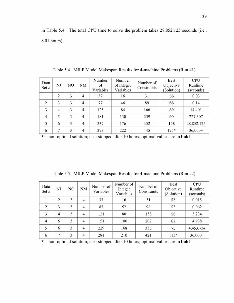
139
in Table 5.4. The total CPU time to solve the problem takes 28,852.125 seconds (i.e.,
8.01 hours).
Table 5.4. MILP Model Makespan Results for 4-machine Problems (Run #1)
Data Set # NJ NO NM
Number of
Variables
Number of Integer Variables
Number of Constraints
Best Objective (Solution)
CPU Runtime (seconds)
1 2 3 4 37 16 31 56 0.03 2 3 3 4 77 46 89 66 0.14 3 4 3 4 125 84 166 80 14.401 4 5 3 4 181 130 259 90 227.307 5 6 3 4 237 176 352 108 28,852.125 6 7 3 4 293 222 445 195* 36,000+
* = non-optimal solution; user stopped after 10 hours; optimal values are in bold
Table 5.5. MILP Model Makespan Results for 4-machine Problems (Run #2)
Data Set # NJ NO NM Number of
Variables
Number of Integer
Variables
Number of Constraints
Best Objective (Solution)
CPU Runtime (seconds)
1 2 3 4 37 16 31 53 0.015
2 3 3 4 83 52 98 53 0.062
3 4 3 4 121 80 158 56 3.234
4 5 3 4 151 100 202 62 4.938
5 6 3 4 229 168 336 75 4,453.734
6 7 3 4 281 210 421 113* 36,000+ * = non-optimal solution; user stopped after 10 hours; optimal values are in bold

140
Table 5.6. MILP Model Makespan Results for 4-machine Problems (Run #3)
Data Set # NJ NO NM Number of
Variables
Number of Integer
Variables
Number of Constraints
Best Objective (Solution)
CPU Runtime (seconds)
1 2 3 4 35 14 27 52 0.016
2 3 3 4 67 36 69 54 0.047
3 4 3 4 113 72 139 59 1.078
4 5 3 4 183 132 254 66 78.297
5 6 3 4 245 184 359 69 9,603.281
6 7 3 4 301 230 455 87* 36,000+ * = non-optimal solution; user stopped after 10 hours; optimal values are in bold
Although the optimal makespan value is achieved for the 6-job problems, the time
required to do it may take up to 8 hours – this comprises an entire work shift in the real
world. This may be fine for the scenario where a new schedule is not needed until the
next day and the data can be run overnight; however, if a machine breaks down and all
the jobs need to be rescheduled immediately, this method is too expensive in terms of
time. In fact, much time would be wasted in determining an optimal value when using an
exact method such as a 0-1 MILP formulation for such problems; thus, another
methodology (such as the TS Algorithm) becomes very useful for finding optimal or
near-optimal results in a more time effective manner. Table 5.7 shows the average
solutions obtained by the 0-1 MILP model for the test cases with 3 to 6 jobs.
For each of the three runs, an attempt was made to solve the 7-job problem with 3
operations and 4 machines. Each problem was run for 36,000 seconds (10 hours), but the
optimal solution was never achieved within this time frame. In addition, 2-job problems
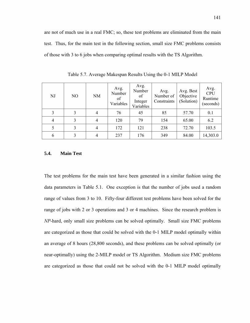
141
are not of much use in a real FMC; so, these test problems are eliminated from the main
test. Thus, for the main test in the following section, small size FMC problems consists
of those with 3 to 6 jobs when comparing optimal results with the TS Algorithm.
Table 5.7. Average Makespan Results Using the 0-1 MILP Model
NJ NO NM
Avg. Number
of Variables
Avg. Number
of Integer
Variables
Avg. Number of Constraints
Avg. Best Objective (Solution)
Avg. CPU
Runtime (seconds)
3 3 4 76 45 85 57.70 0.1
4 3 4 120 79 154 65.00 6.2
5 3 4 172 121 238 72.70 103.5
6 3 4 237 176 349 84.00 14,303.0
5.4. Main Test
The test problems for the main test have been generated in a similar fashion using the
data parameters in Table 5.1. One exception is that the number of jobs used a random
range of values from 3 to 10. Fifty-four different test problems have been solved for the
range of jobs with 2 or 3 operations and 3 or 4 machines. Since the research problem is
NP-hard, only small size problems can be solved optimally. Small size FMC problems
are categorized as those that could be solved with the 0-1 MILP model optimally within
an average of 8 hours (28,800 seconds), and these problems can be solved optimally (or
near-optimally) using the 2-MILP model or TS Algorithm. Medium size FMC problems
are categorized as those that could not be solved with the 0-1 MILP model optimally
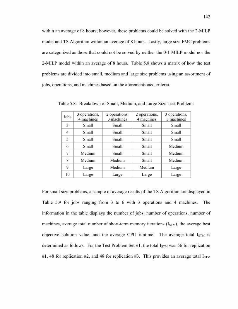
142
within an average of 8 hours; however, these problems could be solved with the 2-MILP
model and TS Algorithm within an average of 8 hours. Lastly, large size FMC problems
are categorized as those that could not be solved by neither the 0-1 MILP model nor the
2-MILP model within an average of 8 hours. Table 5.8 shows a matrix of how the test
problems are divided into small, medium and large size problems using an assortment of
jobs, operations, and machines based on the aforementioned criteria.
Table 5.8. Breakdown of Small, Medium, and Large Size Test Problems
Jobs 3 operations, 4 machines
2 operations, 3 machines
2 operations, 4 machines
3 operations, 3 machines
3 Small Small Small Small 4 Small Small Small Small 5 Small Small Small Small 6 Small Small Small Medium 7 Medium Small Small Medium 8 Medium Medium Small Medium 9 Large Medium Medium Large
10 Large Large Large Large
For small size problems, a sample of average results of the TS Algorithm are displayed in
Table 5.9 for jobs ranging from 3 to 6 with 3 operations and 4 machines. The
information in the table displays the number of jobs, number of operations, number of
machines, average total number of short-term memory iterations (ISTM), the average best
objective solution value, and the average CPU runtime. The average total ISTM is
determined as follows. For the Test Problem Set #1, the total ISTM was 56 for replication
#1, 48 for replication #2, and 48 for replication #3. This provides an average total ISTM

143
value of 50.67 iterations. The average CPU runtime shows the average time it takes for
the TS Algorithm to find an initial solution to the final improved solution.
Table 5.9. A Sample of Average Makespan Results Using the TS Algorithm
Test Problem
Set # NJ NO NM
Avg. Total ISTM
Avg. Best Objective (Solution)
Avg. CPU
Runtime (seconds)
1 3 3 4 50.67 61.00 0.871 2 4 3 4 43 68.00 0.361 3 5 3 4 48 75.70 0.189 4 6 3 4 58.67 88.00 7.849
The results from the TS Algorithm and the 2-MILP have been compared with the optimal
solutions from the 0-1 MILP model in Table 5.10. The small size FMC problem category
includes the range of 3 to 6 jobs with 3 operations and 4 machines, and 6 to 7 jobs with 2
operations and 3 or 4 machines. Medium size problems include the range of 7 to 8 jobs
with 3 operations and 4 machines, 6 to 7 jobs with 3 operations and 3 machines, and 8 to
9 jobs with 2 operations and 3 or 4 machines. The large size problems include the range
of 9 to 10 jobs with 2 to 3 operations, and 3 to 4 machines in this research.
In Table 5.10, the average solution values and average CPU runtime for the TS
Algorithm and 0-1 MILP model, as well as the average relative error (Avg. RE) values
are presented. In addition, the results of the 2-MILP model (from Section 3.6) as well as
the INIT procedure (the initial makespan results at the end of Stage II) have been
compared with the 0-1 MILP model and are also reported in the table.

144
Table 5.10. Results for Small-size FMC Problems of the TS Algorithm, 0-1 MILP Model, 2-MILP Model and INIT Procedure
NJ NO NM AVG MSMILP
AVG CPU Runtime for MILP (seconds)
AVG MS2-MILP
AVG CPU Runtime
for 2-MILP
(seconds)
AVG RE
(2-MILP vs. MILP)
AVG MSINIT
AVG CPU
Runtime for INIT (seconds)
AVG RE
(INIT vs. MILP)
AVG MSINIT
AVG CPU Runtime for TS
(seconds)
AVG RE
(TS vs. MILP)
3 3 4 65.00 0.101 76.00 0.037 16.92% 73.67 0.020 13.33% 65.33 0.871 0.51%
4 3 4 73.33 5.307 76.67 0.063 4.55% 81.33 0.023 10.91% 75.67 0.361 3.18%
5 3 4 81.00 141.412 82.67 0.153 2.06% 87.33 0.072 7.82% 81.67 0.189 0.82%
6 3 4 84.00 14303.047 87.00 0.968 3.57% 111.33 0.023 32.54% 88.00 7.849 4.76%
6 2 3 87.33 74.120 87.67 0.370 0.38% 96.67 0.020 10.69% 90.00 3.301 3.05%
7 2 4 82.33 59.929 82.33 0.179 0.00% 83.67 0.023 1.62% 83.67 0.023 1.62%
144.
145
When comparing the 0-1 MILP model makespan solutions with those achieved using the
TS Algorithm, the TS Algorithm fared very well. The overall average relative error
(Avg. RE) for the small size FMC problems (all three data sets) was determined to be
2.33%, with the Avg. RE for all jobs ranging from 0.51% to 4.76% for the TS Algorithm.
The 2-MILP model’s results had range from 0% to 16.92% for its average relative error,
with an overall average of 4.58% while the INIT procedure yielded an overall average
RE of 12.82% with a range from 1.62 to 32.54%.
For most instances, the CPU runtime for the TS Algorithm are significantly smaller than
those of the 0-1 MILP model, and only a few instances when compared to the 2-MILP
model. The time-savings are a significant factor between the two MILP methods. The 0-
1 MILP model CPU runtime values ranged from an average of 0.101 to 14,303 seconds
with an average of 2430.652 seconds and the 2-MILP model values ranged from 0.037 to
0.968 seconds with an average of 0.295 seconds, while the TS Algorithm values only
ranged from an average of 0.023 to 7.849 seconds with an average of 2.099. Thus, while
the TS Algorithm may not be able to solve every small size FMC problem optimally, it
solves the test problems within 2.33% of the optimal value on the average overall in
substantially less time.
For medium-to-large size FMC problems, the results from the TS Algorithm have been
compared with the solutions provided from the 2-MILP model (when possible), and also
with the initial solution from Stage I (i.e., INIT procedure). In addition, the lower bound

146
(LB) of the makespan was used to help gauge the quality of the solution for these
medium-to-large test problems, especially since optimality is not certain when solving the
problems using the 2-MILP model. Recall from Section 3.6 that this model used relaxed
precedence constraints in its first stage; thus, optimality is not guaranteed during its
second stage. However, the solutions should remain somewhat close those of the 0-1
MILP model on the average. The equation for the LB is as follows:
M
PLB
M
kijkji
∑== 1 ,
}{min (5.1)
Table 5.11 provides the average solutions and CPU runtime for the TS Algorithm and 2-
MILP model for medium size problems, as well as the average relative error (Avg. RE).
In addition, the results of the 2-MILP model and the initial makespan results from Stage I
are also reported in the table.
The overall average relative error (Avg. RE) from the LB for the medium size FMC
problems (all three data sets) was determined to be 8.18%, with the Avg. RE for all jobs
ranging from 5.29% to 10.94% for the TS algorithm. The 2-MILP model yielded an
overall Avg. RE of 8.95% from a range of 4.79 to 11.85%. The INIT procedure yielded
results with an Avg. RE ranging from 10.94 to 38.81% for an overall average of 20.84%
at the end of Stage I. Thus, the TS Algorithm gives a slight advantage over the 2-MILP
model with respect to the makespan results.

147
Table 5.11. Results for Medium-size FMC Problems of the TS Algorithm, 2-MILP Model and INIT Procedure
NJ NO NM AVG LB
AVG MS2-MILP
AVG CPU Runtime
for 2-MILP
(seconds)
AVG RE
(2-MILP vs. LB)
AVG MSINIT
AVG CPU
Runtime for INIT (seconds)
AVG RE
(INIT vs. LB)
AVG MSTS
AVG CPU
Runtime for TS
(seconds)
AVG RE
(TS vs. LB)
AVG MSMILP
7 3 4 93.67 100.00 50.200 6.76% 111.33 0.172 18.85% 100.00 7.905 6.76% 28,800+
8 3 4 100.67 111.70 7595.422 10.96% 118.00 0.027 17.21% 106.00 13.842 5.29% 28,800+
8 2 3 97.33 102.00 48.943 4.79% 113.00 0.020 16.10% 104.33 6.733 7.19% 28,800+
9 2 4 88.33 95.67 13.000 8.30% 98.00 0.155 10.94% 98.00 0.155 10.94% 28,800+
6 3 3 111.67 124.00 62.521 11.04% 155.00 0.030 38.81% 122.00 7.568 9.25% 28,800+
7 3 3 121.00 135.33 1205.271 11.85% 149.00 0.027 23.14% 132.67 3.275 9.64% 28,800+
. 147

148
Table 5.12. Results for Large-size FMC Problems of the TS Algorithm and the INIT Procedure w.r.t. Lower Bound
NJ NO NM AVG LB AVG MSINIT
AVG CPU
Runtime for INIT (seconds)
AVG RE
(INIT vs. LB)
AVG MSTS
AVG CPU
Runtime for TS
(seconds)
AVG RE
(TS vs. LB)
AVG MSMILP
AVG MS2-MILP
9 3 4 122.67 139.00 0.030 13.32% 133.67 2.641 8.97% 28,800+ 28,800+
10 3 4 131.67 159.33 0.030 21.01% 140.33 8.449 6.58% 28,800+ 28,800+
9 3 3 165.67 203.00 0.023 22.54% 180.00 15.662 8.65% 28,800+ 28,800+
10 3 3 185.67 218.67 0.111 17.77% 195.33 8.328 5.21% 28,800+ 28,800+
10 2 3 123.33 137.33 0.118 11.35% 129.33 5.069 4.86% 28,800+ 28,800+
10 2 4 90.67 103.00 0.027 13.60% 99.67 3.345 9.93% 28,800+ 28,800+
148.
149
Once again, the average CPU runtime values for the TS Algorithm were substantially
smaller than those of the 2-MILP model for the medium size FMC problems. For the
medium size problems, the TS Algorithm found solutions from a range of 0.155 to
13.842 seconds on average with an overall average of 6.58 seconds, while the 2-MILP
model ranged from 13.00 to 7,595.422 seconds on average with an overall average of
1495.893 seconds. Thus, even when comparing the TS Algorithm to the 2-MILP model,
there is a significant difference in the overall solution time.
Table 5.12 provides the average solutions and CPU runtime for the TS Algorithm and
INIT procedure for large size problems, as well as the average relative error (Avg. RE).In
addition, the results of the initial makespan results from Stage I are also reported in the
table.
The overall average relative error (Avg. RE) from the lower bound (LB) for the large size
FMC problems (all three data sets) was determined to be 7.37%, with the Avg. RE for all
jobs ranging from 4.86% to 9.93% for the TS algorithm. The INIT procedure yielded
results with an Avg. RE ranging from 11.35 to 22.54% at the end of Stage I, giving an
overall average of 16.60%. Thus, the TS Algorithm performed well with respect to the
LB as well.
The average CPU runtime values for the TS Algorithm were substantially smaller than
those of the INIT procedure for the large size FMC problems. For the large size

150
problems, the TS Algorithm found solutions that ranged from 2.641 to 15.662 seconds
with an overall average of 7.249 seconds, while the INIT procedure ranged from 0.030 to
0.118 seconds on average with an overall average of 0.057 seconds.
5.5. Concluding Summary
In conclusion, the power of the TS Algorithm is graphically displayed in Figure 5.1. In
this figure, notice that the average CPU runtime value of the TS Algorithm is
considerably smaller than the average value found using the 0-1 MILP model for small
size FMC problems, and noticeably smaller than the average CPU runtime value of the 2-
MILP model for medium size FMC problems.
The TS Algorithm is an efficient methodology that collectively uses various heuristic
techniques to solve small, medium and large size FMC problems. The computational
results show that the algorithm is effective in achieving near-optimal (and in some cases
optimal) solutions for a wide range of test problems with pre-set parameters for its Stage
II component. With the use of two separate stages, the TS Algorithm is shown to
improve its objective function value while keeping CPU runtime very small. Overall,
this algorithm could be used to solve a variety of FMC problems for a number of jobs to
help to reduce system makespan, reduce computational effort, and determine very good
production schedules.

151
Average CPU Runtimes for Small, Medium,and Large Size FMC Problems
2430.652
0.295
2.099
1495.893
6.58 7.249
0.1
1
10
100
1000
10000
0-1 MILP 2-MILP TS Algorithm
Various Methods
CPU
Run
time
(sec
onds
)
Small size problems
Medium size problems
Large size problems
Log. (Medium size problems)
Figure 5.1. Average CPU Runtime Comparison for All Methods

152
Chapter 6
SUMMARY AND FUTURE RESEARCH
6.1. Summary
This research has addressed the problem of routing and scheduling a FMC in a single
facility. The primary objective in this research was to develop a methodology that
minimizes the manufacturing makespan within a FMS environment, while reducing the
time that is required to develop and produce a realistic production schedule. Additional
extensions of the MILP model that could be used to minimize the maximum tardiness and
minimize the absolute deviation of meeting due dates were also discussed.
In order to achieve the primary research objective, the following developments were
undertaken:
1. In the first portion of this research, a formal mathematical model was formulated
and used as a starting point for determining FMS schedules. The objective in this
model was to minimize manufacturing makespan for jobs processed in a FMC
environment. The model’s objective function was characterized for solvability in
terms of size (e.g., jobs, operations, and machines). This was performed using a
commercially available optimization software tool called LP_Solve. The initial
preliminary test problems consisted of using small processing times with at most
nine jobs, three operations, and four machines. Later on, the problem is scaled up
153
to a larger processing times and various number of jobs, operations, and available
machines (see Sections 3.4 and 5.4 for details).
2. In the second portion of this research, a two-stage algorithm was created to solve
various instances of the problem in a more time efficient manner since the formal
mathematical model is NP-hard. The two-stage algorithm was coded using
Microsoft Visual C++ .NET on a Pentium 4 2.0GHz computer workstation.
Several test problems were solved, including those problems solved with the exact
MILP mathematical model (see Chapter 4 for details).
3. In the last portion of this research, the effectiveness of the newly proposed
methodology (i.e., the TS Algorithm) versus the NP-hard mixed integer linear
programming (MILP) mathematical model was demonstrated. In order to
accomplish this, an experimental comparison was performed using several test
problems of various system sizes (i.e., changing the number of jobs, operations,
and machines), and an examination of the FMC was conducted using the
makespan performance measure. Small/medium/large size problems were
compared using the results of the developed 0-1 MILP model solved with the
LP_Solve optimization software against the results from the C++ coded TS
Algorithm. These were also compared with the 2-MILP model and the INIT
procedure for the problems that could not be solved optimally within an average
of 8 hours. It was shown that the TS Algorithm found optimal solutions for
several of the problems. For the small-size problems that had optimal makespan

154
solutions, the TS Algorithm was within 2.33% of the optimum makespan solution
values on the overall average and the CPU runtime was substantially smaller.
6.2. Contributions
The following contributions result from this study:
• New 0-1 mixed integer linear programming (MILP) models were developed for
the M-machine, N-job scheduling problem within a FMC, and these models were
utilized for solving small size problems optimally.
• A two-stage MILP model (i.e., 2-MILP model) was developed for solving the
FMC scheduling problem by splitting the original 0-1 MILP model into two sub-
problems: (1) the first for sub-problem solves the routing problem, while (2) the
second solves the sequencing problem. This model was utilized for solving small
and medium size FMC problems.
• An efficient algorithm (i.e., the TS Algorithm) composed of two stages was
developed for solving small, medium and large-scale FMC problems. The first
stage (i.e., the construction phase) incorporates two heuristics that generate initial
feasible job routes and sequences. The first heuristic (i.e., the SPTR Heuristic) is
a newly developed methodology that solves the routing FMC problem, and the
second heuristic (i.e., the VT Heuristic) is a pre-existing heuristic that solves the
sequencing FMC problem. When united together, these two heuristics form Stage
I of the TS Algorithm, and are called the INIT procedure because jointly they
155
produce an initial feasible near-optimal (and sometimes optimal) makespan
solution.
• A novel application of the Tabu Search meta-heuristic procedure was developed
and utilized for the second stage (i.e., improvement phase) of the algorithm.
During this Stage II segment, the Adjacent Pairwise Interchange (API) method is
utilized to find the best job sequences from a neighborhood of the current
solution. In addition, linear programming (LP) formulations are developed and
automatically generated to determine optimal makespan solutions for each job
sequence determined in each neighborhood during the short-term memory phase.
The long-term memory phase of this stage utilizes two procedures (i.e., MOVE
and SWITCH) that are borrowed from the previously mentioned SPTR Heuristic
to change job routes.
6.3. Future Research
Additional FMC scheduling problems could be examined using other regular
performance measures such as maximum tardiness and non-regular performance
measures such as the absolute deviation of due dates using earliness/tardiness penalties.
These will be best examined by using the 0-1 MILP model formulations previously
discussed in Section 3.5 as a basis, then developing a heuristic (or utilize an existing one)
for Stage I, and feed the results into the existing Stage II from this research.
156
The following is a listing of other features that could be added to enhance the future
research of this problem:
• Use other pairwise interchange methods (e.g., Non-Adjacent Pairwise Interchange
- NAPI, Extraction and Forward Shifted Reinsertion – EFSR, and Extraction and
Backward Shifted Reinsertion - EBSR) within the Tabu search procedure of Stage
II
• Use alternative process plans rather than just alternative machines for each job
• Use varying ready times to represent a dynamic FMC versus a static system
• Integrate material handling and storage information as resource constraints for the
0-1 MILP model (which is utilized in the LP sub-problems of Stage II)
• Use varying earliness/tardiness penalties for the earliness/tardiness problems as
discussed in Chapter 3
• Consider more realistic constraints to represent the use of tools, pallets and
fixtures
• Consider performance measures both with and without the no-wait restriction as
discussed in Chapter 3

157
REFERENCES
Agnetis, A., Akfieri, A., Brandimarte, P., and Prinsecchi, P. (1997), Joint job/tool scheduling in a flexible manufacturing cell with no on-board tool magazine. Computer Integrated Manufacturing Systems, 10(1), 61-68. Akturk, M.S. and Avci, S. (1996), Tool allocation and machining conditions optimization for CNC machines. European Journal of Operational Research, 94(2), 335-348. Akturk, M.S. and Ozkan, S. (2001), Integrated scheduling and tool management in flexible manufacturing systems. International Journal of Production Research, 39(12), 2697-2722. Arikan, M. and Erol, S. (2006), Meta-heuristic approaches for part selection and tool allocation in flexible manufacturing systems. International Journal of Computer Integrated Manufacturing, 19(4), 315-325. Asfahl, C.R. (1992), Robots and Manufacturing Automation. John Wiley & Sons, Inc., New York, NY. Atmani, A. and Lashkari, R.S. (1998), A model of machine-tool selection and operation allocation in FMS. International Journal of Production Research, 36(5), 1339-1349. Baker, K. (2000), Elements of Sequencing and Scheduling. Dartmouth College Press, Hanover, NH. Barash, M.M. (1979), Computerized systems in the scheme of things. AIIE Proceedings of the 1979 Fall Industrial Engineering Conference, Houston, TX, 239-246. Basnet, C. (1996), Tabu search heuristic for a loading problem in flexible manufacturing systems. International Journal of Production Research, 34(4), 1171-1174. Basnet, C. and Mize, J.H. (1994), Scheduling and control of flexible manufacturing systems: a critical review. International Journal of Computer Integrated Manufacturing, 7(6), 340-355. Berkelaar, M., Dirks, J., Eikland, K., Notebaert, P., and Gourvest, H. (2004), LPSolve IDE Version 5.1.0.2, Free Software Foundation, Inc., Boston, MA. Bilge, Ü. and Ulusoy, G. (1995), A time window approach to simultaneous scheduling of machines and material handling system in an FMS. Operations Research, 43(6), 1058-1070.

158
Blazewicz, J., Finke, G., Haupt, R., and Schmidt, G. (1988), New trends in machine scheduling. European Journal of Operational Research, 37(3), 303-317. Bryce, A.L.G. and Roberts, P.A. (1982), Flexible manufacturing systems in the U.S.A. Proceedings of the 1st International Conference on Flexible Manufacturing Systems, Brighton, United Kingdom, 49-69. Chan, F.T.S. (2004), Impact of operation flexibility and dispatching rules on the performance of a flexible manufacturing system. International Journal of Advanced Manufacturing Technology, 24(5-6), 447-459. Chan, F.T.S. and Chan, H.K. (2004), A comprehensive survey and future trend of simulation study on FMS scheduling. Journal of Intelligent Manufacturing, 15(1), 87-102. Chan, F.T.S., Chan, H.K., and Lau, H.C.W. (2002), The state of the art in simulation study on FMS scheduling: a comprehensive survey. International Journal of Advanced Manufacturing Technology, 19(11), 830-849. Chan, F.T.S., Kazerooni, A., and Abhary, K. (1997), A fuzzy approach to operation selection. Engineering Applications of Artificial Intelligence, 10(4), 345-356. Chan, F.T.S. and Swarnkar, R. (2006), Ant colony optimization approach to a fuzzy goal programming model for a machine tool selection and operation allocation problem in an FMS. Robotics and Computer-Integrated Manufacturing, 22, 353-362. Chase, C. and Ramadge, P.J. (1992), On real-time scheduling policies for flexible manufacturing systems. IEEE Transactions on Automatic Control, 37(4), 491-496. Clossen, R.J. and Malstrom, E.M. (1982), Effective capacity planning for automated factories requires workable simulation tools and responsive shop floor control. Industrial Engineering, 15, 73-79. Co, H.C. (2001), Managing flexible manufacturing technology: must parts in an FMS always move in a job-shop manner? International Journal of Production Research, 39(13), 2851-2866. Co, H.C., Biermann, J.S., and Chen, S.K. (1990), A methodical approach to flexible-manufacturing-system batching, loading and tool configuration problems. International Journal of Production Research, 28(12), 2171-2186. Croce, F.D. (1995), Generalized pairwise interchanges and machine scheduling. European Journal of Operations Research, 83(2), 310-319.

159
D’Alfonso, T. and Ventura, J. (1995), Assignment of tools to machines in a flexible manufacturing system. European Journal of Operations Research, 81(1), 115-133. Dorigo, M. and Gambardella, L.M. (1997), Ant colony system: a cooperative learning approach to the traveling salesman problem. IEEE Transactions on Evolutionary Computation. 1(1), 53-66. Drake, G., Smith, J.S., and Peters, B.A. (1995), Simulation as a planning and scheduling tool for flexible manufacturing systems. Proceedings of the 1995 Winter Simulation Conference, Arlington, VA, 805-812. French, S. (1982), Sequencing and Scheduling: An Introduction to the Mathematics of the Job-Shop. Wiley, New York, NY. Gamila, M.A. and Motavalli, S. (2003), A modeling technique for loading and scheduling problems in FMS. Robotics and Computer-Integrated Manufacturing, 19(1-2), 45-54. Garey, M.R. and Johnson, D.S. (1979), Computers and Intractibility: A Guide to Theory of NP-Completeness. Freeman, New York, NY. Glover, F. (1989), Tabu search – Part I. ORSA Journal on Computing, 1(3), 190-206. Glover, F. (1990), Tabu search – Part II. ORSA Journal on Computing, 2(1), 4-32. Goswami, M. and Tiwari, M.K. (2006), A reallocation-based heuristic to solve a machine loading problem with material handling constraint in a flexible manufacturing system. International Journal of Production Research, 44(3), 569-588. Guo, Y., Chen, L.-P, Wang, S., and Zhou, J. (2003), A new simulation optimization system for the parameters of a machine cell simulation model. International Journal of Advanced Manufacturing Technology, 21(8), 620-626. Haq, A.N., Karthikeyan, T., and Dinesh, M. (2003), Scheduling decisions in FMS using a heuristic approach. International Journal of Advanced Manufacturing Technology, 22(5-6), 374-379. Harmonosky, C.M. (1990), Implementation issues using simulation for real-time scheduling, control, and monitoring. Proceedings of the 1990 Winter Simulation Conference, New Orleans, LA, 595-598. Harmonosky, C.M. (1995), Simulation-based real-time scheduling: review of recent developments. Proceedings of the 1995 Winter Simulation Conference, Arlington, VA, 220-225.
160
Hatono, I., Yamagata, K., and Tamura, H. (1991), Modeling and on-line scheduling of flexible manufacturing systems using petri-nets. IEEE Transactions on Software Engineering, 17(2), 126-132. Holland, J.H. (1975), Adaptation in Natural and Artificial Systems: An Introductory Analysis with Applications to Biology, Control, and Artificial Intelligence. The University of Michigan Press, Ann Arbor, MI. Holsapple, G.W., Jacob, V.S., Pakath, R., and Zaveri, J.S. (1993), A genetics based hybrid scheduler for generating static schedules in flexible manufacturing contexts. IEEE Transactions on Systems, Man, and Cybernetics, 23(4), 953-972. Hutchison, J. and Chang, Y.-L. (1990), Optimal nondelay job shop schedules. International Journal of Production Research, 28, 245-257. Ibarra, O.H. and Kim, C.E. (1977), Heuristic algorithms for scheduling independent tasks on nonidentical processors. Journal of the Association for Computing Machinery, 24(2), 280-289. Jawahar, N., Aravindan, P., and Ponnambalam, S.G. (1998a), A genetic algorithm for scheduling flexible manufacturing systems. International Journal of Advanced Manufacturing Technology, 14(8), 588-607. Jawahar, N., Aravindan, P., Ponnambalam, S.G., and Karthikeyan, A.A. (1998b), A genetic algorithm-based scheduler for setup-constrained FMC. Computers in Industry, 35(3), 291-310. Jerald, J., Asokan, P., Prabaharan, G., and Saravanan, R. (2005), Scheduling optimization of flexible manufacturing systems using particle swarm optimization algorithm. International Journal of Advanced Manufacturing Technology, 25, 964-971. Jiang, J. and Hsiao, W. (1994), Mathematical programming for the scheduling problem with alternate process plans in FMS. Computers and Industrial Engineering, 27(1-4), 15-18. Joshi, S.B., Mettala, E.G., Smith, J.S., and Wysk, R.A. (1995), Formal models for control of flexible manufacturing cells: physical and system model. IEEE Transactions on Robotics and Automation, 11(4), 558-570. Kim, C.-O., Min, H.-S., and Yih, Y. (1998), Integration of inductive learning and neural networks for multi-objective FMS scheduling. International Journal of Production Research, 36(7), 2497-2509.
161
Kim, Y.W., Inaba, A., Suzuki, T., and Okuma, S. (2001), FMS scheduling based on timed petri net model and RTA* algorithm. Proceedings of the 2001 IEEE International Conference on Robotics and Automation, Seoul, Korea, 848-853. Kirkpatrick, F., Gelatte, C.D., and Vecchi, M.P. (1983), Optimization by simulated annealing. Science, 220, 671-680. Kumar, R., Tiwari, M.K., and Shankar, R. (2003), Scheduling of flexible manufacturing systems: an ant colony approach. Proceedings of the Institute of Mechanical Engineers, Part B: Journal of Engineering Manufacture, 217(10), 1443-1453. Lee, I., Sikora, R., and Shaw, M.J. (1997), A genetic algorithm-based approach to flexible flow-line scheduling with variable lot sizes. IEEE Transactions on Systems, Man, and Cybernetics–Part B: Cybernetics, 27(1), 36-54. Liu, J. and MacCarthy, B.L. (1996), The classification of FMS scheduling problems. International Journal of Production Research, 34(3), 647-656. Liu, J. and MacCarthy, B.L. (1997), A global MILP model for FMS scheduling. European Journal of Operational Research, 100(3), 441-453. Liu, J. and MacCarthy, B.L. (1999), General heuristic procedures and solution strategies for FMS scheduling. International Journal of Production Research, 37(14), 3305-3333. Logendran, R. and Sonthinen, A. (1997), A tabu search-based approach for scheduling job-shop type flexible manufacturing systems. Journal of the Operational Research Society, 48(3), 264-277. Low, C. and Wu, T.-H. (2001), Mathematical modeling approaches to operation scheduling problems in an FMS environment. International Journal of Production Research, 39(4), 689-708. MacCarthy, B.L. and Liu, J. (1993), Addressing the gap in scheduling research: a review of optimization and heuristic methods in production scheduling. International Journal of Production Research, 31(1), 59-79. Masin, M., Shaikh, N.I., and Wysk, R.A. (2003), A parameter variation modeling approach for enterprise optimization. IEEE Transactions on Robotics and Automation, 19(4), 529-542. Min, H.-S., Yih, Y., and Kim, C.-O. (1998), A competitive neural network approach to multi-objective FMS scheduling. International Journal of Production Research, 36(7), 1749-1765.

162
Mohamed, N.S. (1998), Operations planning and scheduling problems in an FMS: an integrated approach. Computers and Industrial Engineering, 35(3-4), 443-446. Morito, S., Lee, K.H., Mizoguchi, K., and Awane, H. (1993), Exploration of a minimum tardiness dispatching priority for a flexible manufacturing system – a combined simulation / optimization approach. Proceedings of the 1993 Winter Simulation Conference, Los Angeles, CA, 829-837. Mukhopadhyay, S.K., Singh, M.K., and Srivasta, R. (1998), FMS machine loading: a simulated annealing approach. International Journal of Production Research, 36(6), 1529-1547. Nof, S.Y., Barash, M.M., and Solberg, J.J. (1979), Operational control of item flow in versatile manufacturing systems. International Journal of Production Research, 17(5), 479-489. Paulli, J. (1995), A hierarchical approach for the FMS scheduling problem. European Journal of Operational Research, 86, 32-42. Perry, C.B. (1969), Variable mission manufacturing systems. Proceedings of the International Conference on Product Development and Manufacturing Technology, University of Strathclyde, Glasgow, Scotland. Potts, C.N. and Whitehead, J.D. (2001), Workload balancing and loop layout in the design of a flexible manufacturing system. European Journal of Operational Research, 129(2), 326-336. Rachamadugu, R. and Stecke, K. (1994), Classification and review of FMS scheduling procedures. Production Planning and Control, 5(1), 2-20. Rodammer, F.A. and White, K.P. Jr. (1988), A recent survey of production scheduling. IEEE Transactions on Systems, Man, and Cybernetics, 18(6), 841-851. Roh, H.-K. and Kim, Y.-D. (1997), Due-date based loading and scheduling methods for a flexible manufacturing system with an automatic tool transporter. International Journal of Production Research, 35(11), 2989-3003. Sabuncuoglu, I. (1998), A study of scheduling rules of flexible manufacturing systems: a simulation approach. International Journal of Production Research, 36(2), 527-546. Sabuncuoglu, I. and Karabuk, S. (1998), A beam search-based algorithm and evaluation of scheduling approaches for flexible manufacturing systems. IIE Transactions, 30(2), 179-191.
163
Sabuncuoglu, I. and Kizilisik, O.B. (2003), Reactive scheduling in a dynamic and stochastic FMS environment. International Journal of Production Research, 41(17), 4211-4231. Sarin, S.C. and Chen, C.S. (1987), Machine loading and tool allocation problem in a flexible manufacturing system. International Journal of Production Research, 25(7), 1081-1094. Sawik, T. (1990), Modelling and scheduling of a flexible manufacturing system. European Journal of Operations Research, 45(2-3), 177-190. Sawik, T. (2004), Loading and scheduling of a flexible assembly system by mixed integer programming. European Journal of Operational Research, 154(1), 1-19. Saygin, C. and Kilic, S.E. (1999), Integrating flexible process plans with scheduling in flexible manufacturing systems. International Journal of Advanced Manufacturing Technology, 15(4), 268-280. Schweitzer, P.J. and Seidman, A. (1991), Optimizing processing rates for flexible manufacturing systems. Management Science, 37(4), 454-466. Shanker, K. and Modi, B.K. (1999), A branch and bound based heuristic for multi-product resource constrained scheduling problem in FMS environment. European Journal of Operational Research, 113(1), 80-90. Sharafali, M., Co, H.C., and Goh, M. (2004), Production scheduling in a flexible manufacturing system under random demand. European Journal of Operational Research, 158(1), 89-102. Smith, J.S. and Peters, B.A. (1998), Simulation as a decision-making tool for real-time control of flexible manufacturing systems. Proceedings of the 1998 IEEE International Conference on Robotics and Automation, Leuven, Belgium, 586-590. Son, Y.J. and Wysk, R.A. (2001), Automatic simulation model generation for simulation-based, real-time shop floor control. Computers in Industry, 45(3), 291-308. Son, Y.J., Wysk, R.A., and Jones, A.T. (2003), Simulation-based shop floor control: formal model, model generation and control interface. IIE Transactions, 35(1), 29-48. Song, A.H., Ootsuki, J.T., Yoo, W.K., Fujii, Y., and Sekiguchi, T. (1995), FMS’s scheduling by colored petri-net model and hopfield neural network algorithm. Proceedings of the 34th SICE Annual Conference, Hokkaido, Japan, 1285-1290.

164
Spur, G. and Mertins, K. (1982), Flexible manufacturing systems in Germany, conditions and development trends. Proceedings of the 1st International Conference on Flexible Manufacturing Systems, Brighton, United Kingdom, 37-47. Srinoi, P., Shayan, E., and Ghotb, F. (2006), A fuzzy logic modeling of dynamic scheduling in FMS. International Journal of Production Research, 44(11), 2183-2203. Srivastava, B. and Chen, W.H. (1996), Heuristic solutions for loading in flexible manufacturing systems. IEEE Transactions on Robotics and Automation, 12(6), 858-868. Starbek, M., Kušar, J., and Brezovar, A. (2003) Optimal scheduling of jobs in FMS. CIRP - Journal of Manufacturing Systems, 32(5), 43-48. Stecke, K.E. (1983), Formulation and solution of nonlinear integer production planning problems for flexible manufacturing systems. Management Science, 29(3), 273-287. Stecke, K.E. and Toczylowski, E. (1992), Profit-based FMS dynamic part type selection over time for mid-term production planning. European Journal of Operations Research, 63(1), 54-65. Swankar, R. and Tiwari, M.K. (2004), Modeling machine loading problem of FMSs and its solution methodology using a hybrid tabu search and simulated annealing-based heuristic approach. Robotics and Computer-Integrated Manufacturing, 20(3), 199-209. Tiwari, M.K. and Vidyarthi, N.K. (2000), Solving machine loading problems in a flexible manufacturing system using a genetic algorithm based heuristic approach. International Journal of Production Research, 38(14), 3357-3384 Tompkins, J.A., and White, J.A. (1984), Facilities Planning. John Wiley & Sons, Inc., New York, NY. Turkcan, A., Akturk, M.S., and Storer, R. (2003), Non-identical parallel CNC machine scheduling. International Journal of Production Research, 41(10), 2143-2168. Ulusoy, G., Sivrikaya-Serifoğlu, F., and Bilge, Ü. (1997), A genetic algorithm approach to the simultaneous scheduling of machines and automated guided vehicles. Computers and Operations Research, 24(4), 335-351. Vancheeswaran, R. and Townsend, M.A. (1993), Two-stage heuristic procedure for scheduling job shops. Journal of Manufacturing Systems, 12(4), 315-325. Weintraub, A., Cormier, D., Hodgson,T., King, R., Wilson, J., and Zozom, A. (1999), Scheduling with alternatives: a link between process planning and scheduling. IIE Transactions. 31(11), 1093-1102.
165
Williams, E.J. and Narayanaswamy, R. (1997), Application of simulation to scheduling, sequencing, and material handling. Proceedings of the 1997 Winter Simulation Conference Proceedings, Atlanta, GA, 861-865. Wu, S.Y.D. and Wysk, R.A. (1988), Multi-pass expert control system – a control/scheduling structure for flexible manufacturing cells. Journal of Manufacturing Systems, 7(2), 107-120. Wu, S.Y.D. and Wysk, R.A. (1989), An application of discrete-event simulation to on-line control in flexible manufacturing. International Journal of Production Research, 27(9), 1603-1623. Yang, J.-B. (2001), GA-based discrete dynamic programming approach for scheduling in FMS environments. IEEE Transactions on Systems, Man, and Cybernetics–Part B: Cybernetics, 31(5), 824-835. Yang, H. and Wu, Z. (2002), GA-based integrated approach to FMS part type selection and machine-loading problem. International Journal of Production Research, 40(16), 4093-4110. Yang, H. and Wu, Z. (2003), The application of adaptive genetic algorithms in FMS dynamic rescheduling. International Journal of Computer Integrated Manufacturing, 16(6), 382-397. Yu, L., Shih, H.M., and Sekiguchi, T. (1999), Fuzzy inference-based multiple criteria FMS scheduling. International Journal of Production Research, 37(10), 2315-2333.

166
APPENDIX
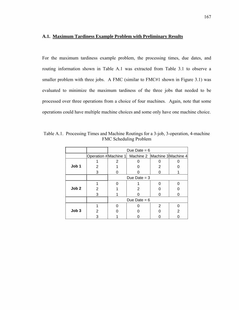
167
A.1. Maximum Tardiness Example Problem with Preliminary Results
For the maximum tardiness example problem, the processing times, due dates, and
routing information shown in Table A.1 was extracted from Table 3.1 to observe a
smaller problem with three jobs. A FMC (similar to FMC#1 shown in Figure 3.1) was
evaluated to minimize the maximum tardiness of the three jobs that needed to be
processed over three operations from a choice of four machines. Again, note that some
operations could have multiple machine choices and some only have one machine choice.
Table A.1. Processing Times and Machine Routings for a 3-job, 3-operation, 4-machine FMC Scheduling Problem
Due Date = 6 Operation # Machine 1 Machine 2 Machine 3 Machine 4 1 2 0 0 0
Job 1 2 1 0 2 0 3 0 0 0 1 Due Date = 3 1 0 1 0 0
Job 2 2 1 2 0 0 3 1 0 0 0 Due Date = 6 1 0 0 2 0
Job 3 2 0 0 0 2 3 1 0 0 0
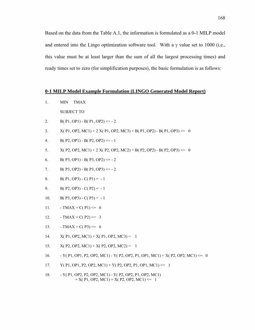
168
Based on the data from the Table A.1, the information is formulated as a 0-1 MILP model
and entered into the Lingo optimization software tool. With a γ value set to 1000 (i.e.,
this value must be at least larger than the sum of all the largest processing times) and
ready times set to zero (for simplification purposes), the basic formulation is as follows:
0-1 MILP Model Example Formulation (LINGO Generated Model Report) 1. MIN TMAX SUBJECT TO 2. B( P1, OP1) - B( P1, OP2) <= - 2 3. X( P1, OP2, MC1) + 2 X( P1, OP2, MC3) + B( P1, OP2) - B( P1, OP3) <= 0 4. B( P2, OP1) - B( P2, OP2) <= - 1 5. X( P2, OP2, MC1) + 2 X( P2, OP2, MC2) + B( P2, OP2) - B( P2, OP3) <= 0 6. B( P3, OP1) - B( P3, OP2) <= - 2 7. B( P3, OP2) - B( P3, OP3) <= - 2 8. B( P1, OP3) - C( P1) = - 1 9. B( P2, OP3) - C( P2) = - 1 10. B( P3, OP3) - C( P3) = - 1 11. - TMAX + C( P1) <= 6 12. - TMAX + C( P2) <= 3 13. - TMAX + C( P3) <= 6 14. X( P1, OP2, MC1) + X( P1, OP2, MC3) = 1 15. X( P2, OP2, MC1) + X( P2, OP2, MC2) = 1 16. - Y( P1, OP1, P2, OP2, MC1) - Y( P2, OP2, P1, OP1, MC1) + X( P2, OP2, MC1) <= 0
17. Y( P1, OP1, P2, OP2, MC1) + Y( P2, OP2, P1, OP1, MC1) <= 1
18. - Y( P1, OP2, P2, OP2, MC1) - Y( P2, OP2, P1, OP2, MC1)
+ X( P1, OP2, MC1) + X( P2, OP2, MC1) <= 1

169
19. Y( P1, OP2, P2, OP2, MC1) + Y( P2, OP2, P1, OP2, MC1) <= 1
20. - Y( P1, OP1, P2, OP3, MC1) - Y( P2, OP3, P1, OP1, MC1) <= - 1
21. Y( P1, OP1, P2, OP3, MC1) + Y( P2, OP3, P1, OP1, MC1) <= 1
22. - Y( P1, OP2, P2, OP3, MC1) - Y( P2, OP3, P1, OP2, MC1) + X( P1, OP2, MC1) <= 0 23. Y( P1, OP2, P2, OP3, MC1) + Y( P2, OP3, P1, OP2, MC1) <= 1 24. - Y( P1, OP1, P3, OP3, MC1) - Y( P3, OP3, P1, OP1, MC1) <= - 1 25. Y( P1, OP1, P3, OP3, MC1) + Y( P3, OP3, P1, OP1, MC1) <= 1 26. - Y( P1, OP2, P3, OP3, MC1) - Y( P3, OP3, P1, OP2, MC1) + X( P1, OP2, MC1) <= 0 27. Y( P1, OP2, P3, OP3, MC1) + Y( P3, OP3, P1, OP2, MC1) <= 1 28. - Y( P2, OP2, P3, OP3, MC1) - Y( P3, OP3, P2, OP2, MC1) + X( P2, OP2, MC1) <= 0 29. Y( P2, OP2, P3, OP3, MC1) + Y( P3, OP3, P2, OP2, MC1) <= 1 30. - Y( P2, OP3, P3, OP3, MC1) - Y( P3, OP3, P2, OP3, MC1) <= - 1 31. Y( P2, OP3, P3, OP3, MC1) + Y( P3, OP3, P2, OP3, MC1) <= 1 32. - 100 Y( P1, OP1, P2, OP2, MC1) - B( P1, OP1) + B( P2, OP2) >= - 98 33. - 100 Y( P2, OP2, P1, OP1, MC1) - X( P2, OP2, MC1) + B( P1, OP1) - B( P2, OP2) >= - 100 34. - 100 Y( P1, OP2, P2, OP2, MC1) - X( P1, OP2, MC1) - B( P1, OP2) + B( P2, OP2) >= - 100 35. - 100 Y( P2, OP2, P1, OP2, MC1) - X( P2, OP2, MC1) + B( P1, OP2) - B( P2, OP2) >= - 100 36. - 100 Y( P1, OP1, P2, OP3, MC1) - B( P1, OP1) + B( P2, OP3) >= - 98 37. - 100 Y( P2, OP3, P1, OP1, MC1) + B( P1, OP1) - B( P2, OP3) >= - 99 38. - 100 Y( P1, OP2, P2, OP3, MC1) - X( P1, OP2, MC1) - B( P1, OP2) + B( P2, OP3) >= - 100 39. - 100 Y( P2, OP3, P1, OP2, MC1) + B( P1, OP2) - B( P2, OP3) >= - 99 40. - 100 Y( P1, OP1, P3, OP3, MC1) - B( P1, OP1) + B( P3, OP3) >= - 98 41. - 100 Y( P3, OP3, P1, OP1, MC1) + B( P1, OP1) - B( P3, OP3) >= - 99 42. - 100 Y( P1, OP2, P3, OP3, MC1) - X( P1, OP2, MC1) - B( P1, OP2) + B( P3, OP3) >= - 100 43. - 100 Y( P3, OP3, P1, OP2, MC1) + B( P1, OP2) - B( P3, OP3) >= - 99 44. - 100 Y( P2, OP2, P3, OP3, MC1) - X( P2, OP2, MC1) - B( P2, OP2) + B( P3, OP3) >= - 100

170
45. - 100 Y( P3, OP3, P2, OP2, MC1) + B( P2, OP2) - B( P3, OP3) >= - 99 46. - 100 Y( P2, OP3, P3, OP3, MC1) - B( P2, OP3) + B( P3, OP3) >= - 99 47. - 100 Y( P3, OP3, P2, OP3, MC1) + B( P2, OP3) - B( P3, OP3) >= - 99 48. - Y( P1, OP2, P3, OP1, MC3) - Y( P3, OP1, P1, OP2, MC3) + X( P1, OP2, MC3) <= 0 49. Y( P1, OP2, P3, OP1, MC3) + Y( P3, OP1, P1, OP2, MC3) <= 1 50. - 100 Y( P1, OP2, P3, OP1, MC3) - 2 X( P1, OP2, MC3) - B( P1, OP2) + B( P3, OP1) >= - 100 51. - 100 Y( P3, OP1, P1, OP2, MC3) + B( P1, OP2) - B( P3, OP1) >= - 98 52. - Y( P1, OP3, P3, OP2, MC4) - Y( P3, OP2, P1, OP3, MC4) <= - 1 53. Y( P1, OP3, P3, OP2, MC4) + Y( P3, OP2, P1, OP3, MC4) <= 1 54. - 100 Y( P1, OP3, P3, OP2, MC4) - B( P1, OP3) + B( P3, OP2) >= - 99 55. - 100 Y( P3, OP2, P1, OP3, MC4) + B( P1, OP3) - B( P3, OP2) >= - 98 56. B( P1, OP1) >= 0 57. B( P2, OP1) >= 0 58. B( P3, OP1) >= 0 59. B( P1, OP2) >= 0 60. B( P1, OP3) >= 0 61. B( P2, OP2) >= 0 62. B( P2, OP3) >= 0 63. B( P3, OP2) >= 0 64. B( P3, OP3) >= 0 65. TMAX >= 0 END 1. INTE Y( P1, OP1, P2, OP2, MC1) 2. INTE Y( P1, OP1, P2, OP3, MC1) 3. INTE Y( P1, OP1, P3, OP3, MC1) 4. INTE Y( P1, OP2, P2, OP2, MC1)

171
5. INTE Y( P1, OP2, P2, OP3, MC1) 6. INTE Y( P1, OP2, P3, OP1, MC3) 7. INTE Y( P1, OP2, P3, OP3, MC1) 8. INTE Y( P1, OP3, P3, OP2, MC4) 9. INTE Y( P2, OP2, P1, OP1, MC1) 10. INTE Y( P2, OP2, P1, OP2, MC1) 11. INTE Y( P2, OP2, P3, OP3, MC1) 12. INTE Y( P2, OP3, P1, OP1, MC1) 13. INTE Y( P2, OP3, P1, OP2, MC1) 14. INTE Y( P2, OP3, P3, OP3, MC1) 15. INTE Y( P3, OP1, P1, OP2, MC3) 16. INTE Y( P3, OP2, P1, OP3, MC4) 17. INTE Y( P3, OP3, P1, OP1, MC1) 18. INTE Y( P3, OP3, P1, OP2, MC1) 19. INTE Y( P3, OP3, P2, OP2, MC1) 20. INTE Y( P3, OP3, P2, OP3, MC1) 21. INTE X( P1, OP2, MC1) 22. INTE X( P1, OP2, MC3) 23. INTE X( P2, OP2, MC1) 24. INTE X( P2, OP2, MC2)
The first set of 65 lines represents the various constraints that are necessary to model the
FMC problem. The second set of 24 lines represents the integer variables that are
required. The example problem was characterized for 6 jobs and the results are shown in
Table A.2. Since it is an NP-hard problem, it is assumed that the number of variables,

172
number of integer variables, and number of constraints will continue to grow as the
problem size increases beyond the 6 jobs. Thus, the CPU Runtime would also increase
beyond 90 seconds as well. Note that the third line in Table A.2 matches the
aforementioned number of constraints and number of integer variables.
Table A.2. Maximum Tardiness Results for a 6-job, 3-operation, 4-machine FMC Scheduling Problem (derived from Table A.1)
Jobs, N
Machines, M
Operations, J(i)
Number of
Variables
Number of
Integer Variables
Number of Constraints
Best Objective (Solution)
CPU Runtime (seconds)
1 4 3 51 2 7 0 < 1 2 4 3 173 12 29 1 < 1 3 4 3 366 24 65 1 < 1 4 4 3 633 42 100 1 < 1 5 4 3 971 72 163 1 < 1 6 4 3 1380 108 232 2 90
The resulting optimal schedule for the example problem is shown in Figure A.1. It
reveals that Job #1 is completed at time 7; thus, it is tardy (i.e., late) by 1 time unit since
it had a due date of 6 time units. Job #2 is completed at time 5 and is also tardy by 1 time
unit because of its due date requirement of 4 time units. Job #3 is completed at time 5
and is not tardy at all; therefore, the maximum tardiness is only one time unit for this
example problem.

173
3 JOBS, 3 OPERATIONS Machine 1 P111 P231 P331 P121 Machine 2 P212 P222 Machine 3 P313 Machine 4 P324 P134
0 1 2 3 4 5 6 7
Time
Figure A.1. Minimum Tardiness Schedule for a 3-job FMS Scheduling Problem (based on data from Table A.1)
A.2. Maximum Tardiness Example Problem with No-Wait Condition
While observing the maximum tardiness objective, suppose the FMC had an additional
requirement that no machine should be kept idle for any period of time in which parts
could be processed immediately for subsequent operations without interruptions. This
would require the no-wait (nondelay) condition (as discussed in section 3.5.3) to be
imposed on the 0-1 MILP model. In addition, since this only requires one inequality
constraint set #(2) to be changed into an equality constraint set #(24), the problem
characterization is identical to that shown in Table A.1. However, the resulting optimal
schedule for this example problem has changed slightly and is shown in Figure A.2. It
reveals that Part #1 is now completed at time 6; thus, it now meets its due date of 6 time
units. Part #2 and Part #3 remained the same – meaning that Part #2 is still tardy by 1
time unit and Part #3 finishes before its due date. Therefore, the maximum tardiness
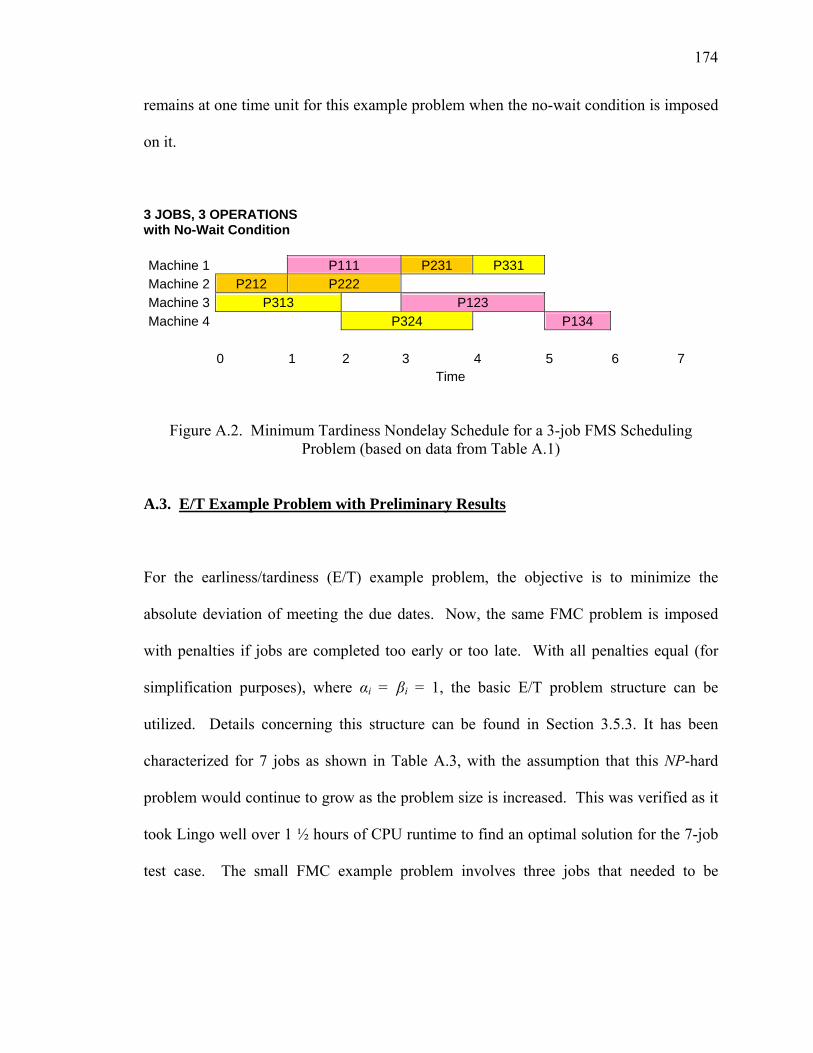
174
remains at one time unit for this example problem when the no-wait condition is imposed
on it.
3 JOBS, 3 OPERATIONS with No-Wait Condition Machine 1 P111 P231 P331 Machine 2 P212 P222 Machine 3 P313 P123 Machine 4 P324 P134
0 1 2 3 4 5 6 7
Time
Figure A.2. Minimum Tardiness Nondelay Schedule for a 3-job FMS Scheduling Problem (based on data from Table A.1)
A.3. E/T Example Problem with Preliminary Results
For the earliness/tardiness (E/T) example problem, the objective is to minimize the
absolute deviation of meeting the due dates. Now, the same FMC problem is imposed
with penalties if jobs are completed too early or too late. With all penalties equal (for
simplification purposes), where αi = βi = 1, the basic E/T problem structure can be
utilized. Details concerning this structure can be found in Section 3.5.3. It has been
characterized for 7 jobs as shown in Table A.3, with the assumption that this NP-hard
problem would continue to grow as the problem size is increased. This was verified as it
took Lingo well over 1 ½ hours of CPU runtime to find an optimal solution for the 7-job
test case. The small FMC example problem involves three jobs that needed to be
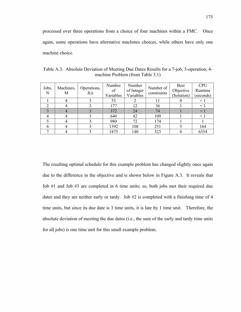
175
processed over three operations from a choice of four machines within a FMC. Once
again, some operations have alternative machines choices, while others have only one
machine choice.
Table A.3. Absolute Deviation of Meeting Due Dates Results for a 7-job, 3-operation, 4-
machine Problem (from Table 3.1)
Jobs, N
Machines, M
Operations, J(i)
Number of
Variables
Number of Integer Variables
Number of constraints
Best Objective (Solution)
CPU Runtime (seconds)
1 4 3 53 2 11 0 < 1 2 4 3 177 12 36 1 < 1 3 4 3 372 24 74 1 < 1 4 4 3 640 42 109 1 < 1 5 4 3 980 72 174 1 1 6 4 3 1392 108 251 5 164 7 4 3 1875 140 323 8 6354
The resulting optimal schedule for this example problem has changed slightly once again
due to the difference in the objective and is shown below in Figure A.3. It reveals that
Job #1 and Job #3 are completed in 6 time units; so, both jobs met their required due
dates and they are neither early or tardy. Job #2 is completed with a finishing time of 4
time units, but since its due date is 3 time units, it is late by 1 time unit. Therefore, the
absolute deviation of meeting the due dates (i.e., the sum of the early and tardy time units
for all jobs) is one time unit for this small example problem.
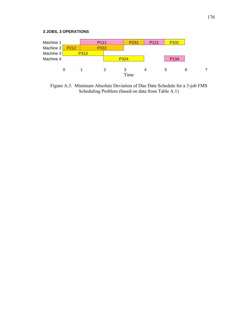
176
3 JOBS, 3 OPERATIONS Machine 1 P111 P231 P121 P331 Machine 2 P212 P222 Machine 3 P313 Machine 4 P324 P134 0 1 2 3 4 5 6 7
Time
Figure A.3. Minimum Absolute Deviation of Due Date Schedule for a 3-job FMS Scheduling Problem (based on data from Table A.1)
VITA
Richard A. Pitts, Jr. was born on July 26, 1969 in Baltimore, Maryland. He received his
B.S. in Industrial Engineering (IE) in May 1991 from Morgan State University (MSU).
After working briefly in industry, Richard returned to MSU to work as a Special Projects
Engineer where he setup, operated and managed the Automation & Robotics Laboratory
in the School of Engineering. He was introduced to teaching at the University level
during this time and decided to return back to school in August 1992. Upon completion
of the M.S. degree in Industrial Engineering at the Pennsylvania State University (PSU),
Richard returned to MSU to become a faculty member of the IE department. During the
next 6 years, Richard taught several courses, advised many students, and was selected for
the Who’s Who Among America's Teachers Award in 1998. Leaving MSU once again,
he returned back to PSU to pursue the Ph.D. degree in Industrial Engineering. He was an
ONR/HBEC Future Faculty Fellow and an ASEE Helen T. Carr Fellow during his Ph.D.
studies. Recently, Richard has been selected to be honored twice in the “The
Chancellor’s List, 2004-2005, and 2005-2006” publications. He is an active member of
the Institute of Industrial Engineers (IIE) and the Society of Manufacturing Engineers
(SME). His research interest includes the following: Industrial Scheduling, Meta-
heuristic Algorithms, Robotics & Automation, Material Handling Systems, and
Simulation.