A Macroscopic Plasma Lagrangian and its Application to ... · A Macroscopic Plasma Lagrangian and...
262
A Macroscopic Plasma Lagrangian and its Application to Wave Interactions and Resonances by Yueng-Kay Martin Peng June 1974 SUIPR Report No. 575 National Aeronautics and Space Administration Grant NGL 05-020-176 National Science Foundation Grant GK-32788X (NASA-CR-138649) A MACROSCOPIC PLASMA N74-27231 LAGRANGIAN AND ITS APPLICATION TO WAVE INTERACTIOUS AND RESONANCES (Stanford Univ.) 262 p HC $16.25 CSCL 201 Unclas G3/25 41289 INSTITUTE FOR PLASMA RESEARCH STANFORD UNIVERSITY, STANFORD, CALIFORNIA NIZ~a https://ntrs.nasa.gov/search.jsp?R=19740019118 2018-06-15T10:26:53+00:00Z
Transcript of A Macroscopic Plasma Lagrangian and its Application to ... · A Macroscopic Plasma Lagrangian and...

A Macroscopic Plasma Lagrangianand its Application to WaveInteractions and Resonances
by
Yueng-Kay Martin Peng
June 1974
SUIPR Report No. 575
National Aeronautics and Space AdministrationGrant NGL 05-020-176
National Science FoundationGrant GK-32788X
(NASA-CR-138649) A MACROSCOPIC PLASMA N74-27231LAGRANGIAN AND ITS APPLICATION TO WAVEINTERACTIOUS AND RESONANCES (StanfordUniv.) 262 p HC $16.25 CSCL 201 Unclas
G3/25 41289
INSTITUTE FOR PLASMA RESEARCHSTANFORD UNIVERSITY, STANFORD, CALIFORNIA
NIZ~a
https://ntrs.nasa.gov/search.jsp?R=19740019118 2018-06-15T10:26:53+00:00Z

A MACROSCOPIC PLASMA LAGRANGIAN AND ITS APPLICATION TO WAVEINTERACTIONS AND RESONANCES
by
Yueng-Kay Martin Peng
National Aeronautics and Space AdministrationGrant NGL 05-020-176
National Science FoundationGrant GK-32788X
SUIPR Report No. 575
June 1974
Institute for Plasma ResearchStanford UniversityStanford, California
I
A MACROSCOPIC PLASMA LAGRANGIAN AND ITS APPLICATION TO WAVEINTERACTIONS AND RESONANCES
by
Yueng-Kay Martin PengInstitute for Plasma Research
Stanford UniversityStanford, California 94305
ABSTRACT
This thesis is concerned with derivation of a macroscopic plasma
Lagrangian, and its application to the description of nonlinear three-
wave interaction in a homogeneous plasma and linear resonance oscilla-
tions in a inhomogeneous plasma.
One approach to obtain -the--Lagrangian is via the inverse problem
of the calculus of variations for arbitrary first and second order
quasilinear partial differential systems. Necessary and sufficient
conditions for the given equations to be Euler-Lagrange equations of a
Lagrangian are obtained. These conditions are then used to determine
the transformations that convert some classes of non-Euler-Lagrange
equations to Euler-Lagrange equation form. The Lagrangians for a linear
resistive transmission line and a linear warm collisional plasma are
derived as examples.
Using energy considerations, the correct macroscopic plasma
Lagrangian is shown to differ from the velocity-integrated Low Lagrangian,
by a macroscopic potential energy that equals twice the particle thermal
kinetic energy plus the energy lost by heat conduction. The generalized
variables are the macroscopic plasma cell position (Eulerian coordinates)
defined in Lagrangian coordinates, and the vector and scalar potentials
APReC Pr.A. AOpiii" ' TAhi NO)T FED
defined in Eulerian coordinates. With the continuity and heat flow
equations treated as constraints, the Euler-Lagrange equations are shown
to be the force law and Maxwell's equations. The effects of viscosity,
heat conduction, and elastic collisions are included in this variational
principle. The corresponding macroscopic Hamiltonian, and the micro-
scopic Hamiltonian corresponding to the Low Lagrangian, are also derived.
Under the assumptions of scalar pressure and adiabatic processes,
the macroscopic Lagrangian is approximated by expansions in weak pertur-
bations of the generalized variables. The averaged Lagrangian method
is then used to derive nonlinear three-wave coupling coefficients in a
warm homogeneous two-component plasma. The effects of wave damping
are included phenomenologically in the coupled mode equations. The
general results are then specialized to make detailed quantitative
comparisons between theory and available experimental results on parame-
trically excited ion-acoustic waves.
The approximate quadratic Lagrangian is also used to estimate the
electrostatic (Tonks-Dattner) resonance properties of an inhomogeneous
plasma. The Rayleigh-Ritz procedure is applied directly to the Lagrangian
corresponding to a system of Euler-Lagrange equations. Use of an appro-
priate set of trial functions then leads to frequency and eigenfunction
estimates in excellent agreement with the existing theoretical and experi-
mental results for a low pressure positive column. Since this method
mainly involves evaluating finite integrals, and solving algebraic eigen-
value equations, it is found to be more efficient than numerically solving
differential equations, and more accurate than inner-outer expansions.
iv

TABLE OF CONTENTS
Page
ABSTRACT. . . . . . . . . . . . .......................... iii
LIST OF TABLES. . . . . ...... . . . . ...... . viii
LIST OF ILLUSTRATIONS . ... ... . ............ ix
LIST OF SYMBOLS . . ....... . . . . . . . . .* xvi
ACKNOWLEDGMENTS . . . . . . . . . * * * * xl
1. INTRODUCTION . . . . . . . ........................1
2. INVERSE PROBLEM OF THE CALCULUS OF VARIATIONS . ........
2.1 Introduction . .............. . . . .. . . 52.2 First Order Differential Equations .... ....... 7
2.2.1 Necessary Conditions . . . . ... ...... .. 82.2.2 Sufficient Conditions ...... . . . . . . . 9
2.2.3 Linear Differential Equations . .. . ...... 122.3 Second Order Differential Equations. . .......... 13
2.3.1 Necessary Conditions ... ..... ..... . 142.3.2 Sufficient Conditions .............. 15
2.3.3 Nonlinear Differential Equations of theSecond Rank .. ..... . o o ...... ....... 18
2.4 Differential Transformations . . o ....... ... 212.4.1 Differential Transformation of Linear
Differential Equations. ........... 222.4.2 Resistive Transmission Line . . . . ........... o 232.4.3 Warm Collisional Plasma .............. 25
2.5 Discussion . . . . ....................... 28
3. LAGRANGIAN AND HAMILTONIAN DENSITIES FOR PLASMAS. ... ...... 313.1 Introduction . . . . . . ..................... 31
3.2 Lagrangian Density . ...... . . .. ............ .. 363.2.1 Macroscopic Approximation to the Low
Lagrangian. . . . . . . . . . .37
3.2.2 Macroscopic Potential, U . ............ 423.2.3 Application of Hamilton's Principle ..... . . 46
v

Page
3.3 Hamiltonian Density. . . . . . . . . . . . . . . . . . . 56
3.3.1 Lagrangian Coordinates, , . . . . . . . . . . . 57
3.3.2 Modified Legendre Transformation . . . . . . . . 61
3.3.3 Hamilton Equations. ..... . . . . . . . . . . . . 63
3.3.4 Poisson Brackets. . . . . . . . . . . . .. . . . 65
3.3.5 Energy Conservation Equation. . . . . . . . . . . 67
3.3.6 Microscopic Hamiltonian Density . . . . . . . . . 69
3.3.7 Entropy for Plasmas . . . . . . . . . . . . . . . 73
3.4 Discussion of the Macroscopic Potential, . . . . . . . 74
3,4.1 Relation of U to Viscosity and HeatConduction . . . . . . . . . . . . . . . . . . . . 75
3.4.2 Loss of Particle Discreteness in ApplyingMacroscopic Approximation . . . .... . . . . . . 76
3.4.3 Definition of Plasma Cell Boundary. .. . . . . . 78
3.4.4 Relations Among the Variational Principles ofVarious Models. . ................ . 79
3.5 Discussion .................... . . . . 81
4. THREE-WAVE INTERACTIONS: THEORY . . .............. . 84
4.1 Introduction ................... . . . . 84
4.2 Perturbation Approximation to L . ........... 86
4.2.1 Definition of Perturbations . . . . . . . . . . . 87
4.2.2 Expansions of , , n ', P . ....... ........ . 89
4.2.3 Expansion of the Lagrangian . . . . . . . . . . . 934.3 Nonlinear Wave Coupling Coefficients . . . . . . . . . . 96
4.3.1 Averaged Lagrangian . .............. 96
4.3.2 Linear Waves . ................. . 99
4.3.3 Wave Coupling Coefficients . . . . . . . . . . . 100
4.4 Parametric Wave Amplification . ............ . 104
4.4.1 Parametric Amplification Without WaveDamping .. ................ .. . 105
4.4.2 Wave Damping. . . .j..... ....... . . .. 112
4.4.3 Effects of Other Nonlinear Processes andPlasma Inhomogeneity ............... . 120
4./ Discussion . . . . . . . . . . . . . . . . . . . . . . . 125
vi

Page
THREE-WAVE INTERACTION: APPLICATIONS ..... ..... . . ...126
5.1 Introduction• ............ . . . .... . .126
5.2 Nonlinear Interaction of Ion-Acoustic Waves . . . ... .133
5.2.1 The Experiment and Interpretation . ..... .. 133
5.2.2 Ion-Acoustic Waves (I) and CouplingCoefficient: 0 = 0 *....... ... .. . . . . . 139
5.2.3 Dependence of ZO on e (0) ............ .141
5.3 Excitation of an Ion-Acoustic Wave by Two ElectronPlasma Waves ... ....... . . ..... . . . . . . .1445.3.1 Electron Plasma Waves (P) and Coupling
Coefficients: 8 = 0 ....... . . . . ....144
5.3.2 Evolution of Fi and es ....... . . . . .146
5.4 Excitation of an Ion-Acoustic Wave by Two Whistlers:Collinear Propagation . . ..... . . .. . ........... 148
5.4.1 Experimental Observations. ..... . ..... 149
5.4.2 Whistler Waves (R) and the CouplingCoefficient: 0 =,0 . ...... . . . . . . . ...... 192
5.4.3 Evolution of i and es . ........ .. 154Excitation of an Ion-Acoustic Wave by TwoWhistlers:Oblique Propagation .. . . . . . . . ................. 1975.5.1 Obliquely Propagating Ion-Acoustic Waves (I").
K" = [K" 0, K" . . 1585.5.2 Obliquely Propagating Whistlers (R ),K = Kx O, Kj . . . . . . . . . . . . . . . .160
5..3 Synchronism Conditions and CouplingCoefficient ..... . . . . .............. . 161
,.,.4 Evolution of 8. and s . . . . . .1645.6 Discussion........ . . . . . . . .. . . . .167
6. CONCLUSIONS. . . . . .. . . . .............. . . . . . . 169
REFERENCES ........ . . . . ................ . . .174
APPENDIX A SOLUTION OF ULTRAHYPERBOLIC EQUATIONS . ... .. .181
APPENDIX B VARIATIONAL CALCULATIONS FOR RESONANCEOSCILLATIONS OF INHOMOGENEOUS PLASMASby Y-K. M. Peng and F.W. Crawford
vii
LIST OF TABLES
Number Page
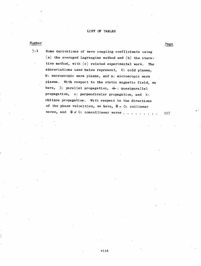
5.1 Some derivations of wave coupling coefficients using
(a) the averaged Lagrangian method and (b) the itera-
tive method, with (c) related experimental work. The
abbreviations used below represent, C: cold plasma,
M: macroscopic warm plasma, and m: microscopic warm
plasma. With respect to the static magnetic field, we
have, II: parallel propagation, -1-: quasiparallel
propagation, 1: perpendicular propagation, and X:
oblique propagation. With respect to the directions
of the phase velocities, we have, = 0: collinear
waves, and ® 0: noncollinear waves . . . . . . ... . 127
viii

LIST OF ILLUSTRATIONS
Figure Page
2.1 Resistive transmission line. . .............. . 24
3.1 In phase space, a particle trajectory (-) can be
specified by its Lagrangian (initial) coordinates,
( O0,0,0), or its Eulerian (present) coordinates,
(x,v,t). The polarization vector, , used by
Sturrock (1958), connects the real particle trajec-
tory (---) to a specified trajectory (--) ........ 32
3.2 Particles of a species that occupy a spatial volume
V at time t are assumed to occupy a volume V0
at t = 0. This approximation is acceptable when t
is sufficiently close to t = 0 ... . . . . . . . . . 39
3.3 The size of AV is assumed to be much larger than
the particle mean free path so that the same
particles of a species are contained in AV for
a time period much larger than the mean particle
transit time across AV. This assumption of large
AV size enables us to justify the necessary correc-
tion to the v-integrated Low Lagrangian. It will
be seen in Section 3.5 that the large size assumption
is not necessary for the Lagrangian of (3.22). . ..... . 44
3.4 The definition of nonlocal and local variations in
n due to the virtual displacement ((x,t). The
nonlocal variation, 68n, is defined by comparing
n with n for the same cell, while the local
variation, 6n, is for the same coordinate x, before
and after the virtual displacement. The trajec-
tories of the same cell before and after virtual
displacement are denoted by -- and ---, respec-
tively . ...... . . .......... ... ...... .
ix

LIST OF ILLUSTRATIONS (cont.)
Figure Page
3.5 The definition of nonlocal and local variations in
zD due to the virtual displacement (xt). The
nonlocal variation, 8 is obtained by com-
paring D with vD for the same cell, while the
local variation, 6v D) is for the same coordinate x.
The trajectories of the same cell before and after
virtual displacement are denoted by -- and ---,
respectively. The virtually displaced trajectory
that passes through (xt) is denoted by
. .. . . . . . . . ,. . . . .. . . . . . . . .5 1
3.6 The approach of a real displacement, Ax, performed
in a short time period, At, to the virtual dis-
placement, , as At diminishes to zero. Since
(3.29) describes the changes in n and Tr P/2
along the path Ax, the virtual displacements in
n and Tr P/2 are then described by (3.29) as a
special case when At - 0 and Ax . ....... . . . .. 2
3.7 The conceptual difference between the cells of the
(a) microscopic and (b) macroscopic models in a
collisionless plasma. The arrows in (a) indicate
the motions of the particles that carry the boundary
surfaces of dx with them. In (b), do is the
surface area of dx with an outward normal. The
cell, d,, in the macroscopic model, can only move
with the macroscopic drift, yD. The particle thermal
motion then gives rise to momentum and energy
transfer across do . . . . . .. . . . . . . . . . . . . 72
x

LIST OF ILLUSTRATIONS (cont.)
Figure Page
3.8 Relations among the variational principles of various
plasma models. Here LT and H T represent the
total Lagrangian and Hamiltonian, respectively, in
the collisional microscopic model; LL and HL,represent the (Low) Lagrangian and Hamiltonian,
respectively, in the collisionless microscopic
model; H.P. represents Hamilton's principle; L.T.
represents the Legendre transformation, and E.C.E.
represents the total energy conservation equation. .... . 80
4.1 The definition of perturbation in the macro-
scopic plasma cell position from x to x'.
The perturbation is performed in such a way that
the number of particles of a Species in the cell
is fixed. The perturbed and unperturbed cell
trajectories are denoted as - and --- , respec-
tively. The cell velocities before and after
perturbation are denoted by v (x,t) and v (x',t)
respectively. The velocity of the cell that
is at (x,t) after perturbation is denoted by
t) 88v.(.t).................... ...... 88
4.2 The distinction between (a) the co-flow
(forward scatter) and (b) the contra-flow
(back scatter) cases of parametric amplifi-
cation. The solid lines indicate the dis-
persion curves near the (K,) of the pump,
signal, and idler waves. In the co-flow
case, the group velocities (U = dQ/dK) of the
signal and idler have the same sign, while in
the contra-flow case, their group velocities
have opposite signs .. . ............ . . .... 107
xi
LIST OF ILLUSTRATIONS (cont.)
Figure Page
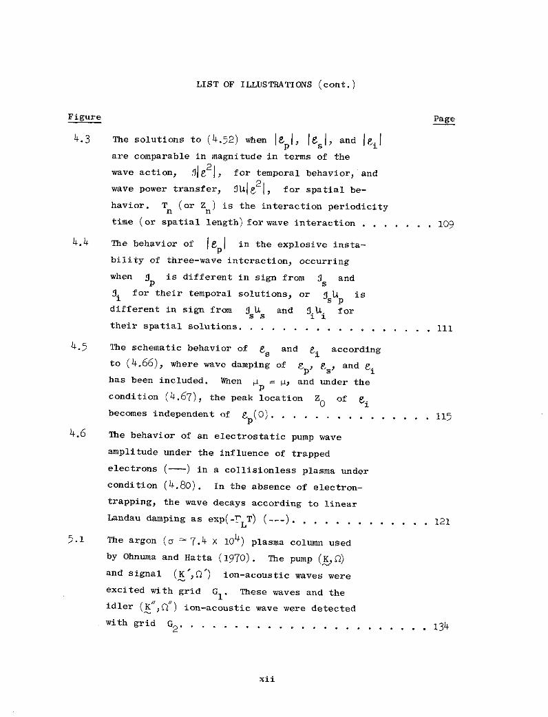
4.3 The solutions to (4.52) when le,1, le, and lil
are comparable in magnitude in terms of the
wave action, ik2 , for temporal behavior, and
wave power transfer, U[le21, for spatial be-
havior. T (or Zn ) is the interaction periodicity
time (or spatial length) for wave interaction . . . .. . . 109
4.4 The behavior of lep in the explosive insta-
bility of three-wave interaction, occurring
when jp is different in sign from Is and
3i for their temporal solutions, or s Up is
different in sign from 3s s and I.51. for
their spatial solutions .. . . . . . . . . . . . . . . . . 111
4.r The schematic behavior of 8s and 8i according
to (4.66), where wave damping of e, gs, and i
has been included. When p = 4, and under the
condition (4.67), the peak location ZO of Fibecomes independent of p (0) . . . . . . . . . . .... . 115
4.6 The behavior of an electrostatic pump wave
amplitude under the influence of trapped
electrons (--) in a collisionless plasma under
condition (4.80). In the absence of electron-
trapping, the wave decays according to linear
Landau damping as exp(-rLT) (---). . . . . . . . . . . . 121
5.1 The argon (o - 7.4 X 10⁴) plasma column used
by Ohnuma and Hatta (1970). The pump (K,2)
and signal (K','0) ion-acoustic waves were
excited with grid G1 . These waves and the
idler (K",Y ) ion-acoustic wave were detected
with grid G2 . * * *. . . . . . * , * . . . . . . . . . 134
xii

LIST OF ILLUSTRATIONS (cont.)
Figure Page
5.2 A typical observation by Ohnuma and Hatta (1970) of
interaction among collinear ion-acoustic waves. The
exciting grid for the pump, 8 , and signal, es,
is located at z = 0. The peak of the idler, e,
is located at z0 .................. . 136
5.3 The measured behavior of 8p for several exciting
voltages,V , at the grid. For z < 4 cm, the
spatial decay rate, p, of P, was found to in-
crease with Vp when Vp > Vth - 2V [Ohnuma
and Hatta (1970), figure 16] . . . . ............. 137
5.4 The dispersion curve for ion-acoustic waves (I)
propagating parallel to the dc magnetic field
under the conditions of (5.6). The synchronism
conditions for nonlinear coupling of three ion-
acoustic waves (p, s, and i) are always satisfied
over its linear portion ....... . . . . . . . . . . 140
5.5 (a) The increase of 4p with the grid exciting
voltage, Vp , for the pump wave, as deduced from
figure 5.3, and their approximate relation.
(b) The dependence of the peak location, Z0,
of the idler, Ei, on the boundary values of the
pump, 8p(0), according to (5.4) and the rela-
tion, ZO ~ 0.7/ p used by Ohnuma and Hatta
(1970) . . . . . . . . . . . . . . . .. . . . . . . . . .143
$.6 Dispersion curves and synchronism conditions
for longitudinal electron plasma (pump and
signal) waves (P) and ion-acoustic (idler)
waves (I) ... . . . . . . . . . ..................... . 145
xiii
LIST OF ILLUSTRATIONS (cont.)
Figure Page
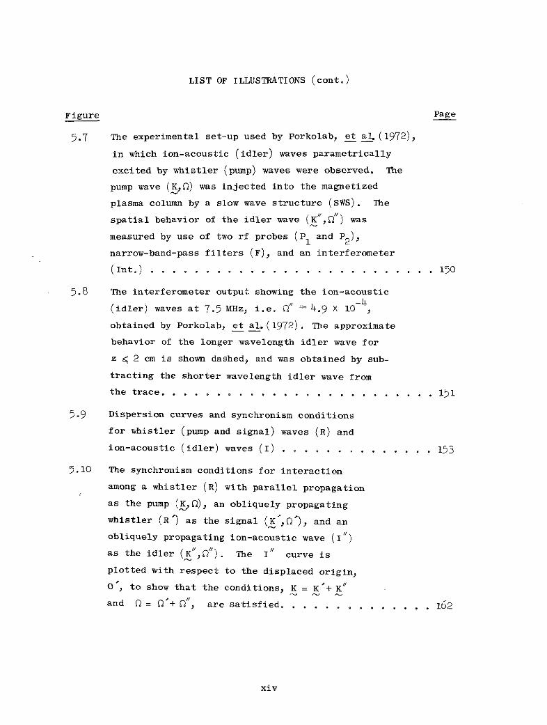
5.7 The experimental set-up used by Porkolab, et al (1972),
in which ion-acoustic (idler) waves parametrically
excited by whistler (pump) waves were observed. The
pump wave (K,2) was injected into the magnetized
plasma column by a slow wave structure (SWS). The
spatial behavior of the idler wave (K ,") was
measured by use of two rf probes (P1 and P2)9
narrow-band-pass filters (F), and an interferometer
(Int.) . . . . . . . . . . . . . . . . . . . . . . .. . . 150
5.8 The interferometer output showing the ion-acoustic• . 1-4
(idler) waves at 7.5 MHz, i.e. 2// 4.9 x 10
obtained by Porkolab, et al.(1972). The approximate
behavior of the longer wavelength idler wave for
z < 2 cm is shown dashed, and was obtained by sub-
tracting the shorter wavelength idler wave from
the trace. . . . . . . . . . . . . . . . . . ..... . 151
5.9 Dispersion curves and synchronism conditions
for whistler (pump and signal) waves (R) and
ion-acoustic (idler) waves (I) .............. 153
5.10 The synchronism conditions for interaction
among a whistler (R) with parallel propagation
as the pump (K.0), an obliquely propagating
whistler (R') as the signal (K ,2'), and an
obliquely propagating ion-acoustic wave (I")
as the idler (K / 2). The I curve is
plotted with respect to the displaced origin,
0 , to show that the conditions, K = K + K"
and R = R+ , are satisfied. .. ....... . . . . . 162
xiv

LIST OF ILLUSTRATIONS (cont.)
Figure Page
5.11 Comparison between the observed evolution of the
short wavelength idler ion-acoustic wave, deduced
from a result obtained by Porkolab, et al.(1972)
(figure 5.8), and the theoretical evolution of
gi(Z), according to (5.48), with ei(0):egs():gingiven approximately as 5:4:1. The theoretical
evolution of the signal whistler wave amplitude,
e,s(Z) is subject to future experimental
verification. . . . . . . . . . . . . . . . . . .. .. . 166
xv

LIST OF SYMBOLS
Symbol Section where used;page of definition
(1) Latin Alphabet
a constant defined in (5.34) 5;159
a arbitrary constant 2;27
a coefficient defined in (2.36) 2;18ij
a coefficient defined in (2.36) 2;18ij
aU1aijk coefficient defined in (2.36) 2;18
ijAij coefficient defined in (2.21) 2;14
A vector potential 2,3,,4;l0
A perturbed vector potential 4;87
Al perturbation vector potential 4;87
AM macroscopic vector potential 3;41
A random vector potential 3;41
a normalized A 4;96
b constant defined in (5.34) 5;159
b arbitrary constant 2;27
b coefficient defined in (2.36) 2;18
b coefficient defined in (2.36) 2;18
b y coefficient defined in (2.36) 2;18
b coefficient defined in (2.36) 2;18
xvi
LIST OF SYMBOLS (cont.)
Symbol Section where used;page of definition
bi coefficient defined in (2.36) 2;18
bij coefficient defined in (2.36) 2;18
B' coefficient defined in (2.21) 2;14
B magnetic field 1,2,3;1
B static magnetic field 4;96
c speed of light in vacuum 4;96
c arbitrary constant 2;27
ci coefficient defined in (2.1) 2;12
C normalized capacitance 2;23
C collision term in Boltzmann equation 3;48
C 1Cpsi 4,5;113
Cij differential transformation operator 2;27
C coefficient defined in (2.1) 2;7
Cpsi nonlinear wave-wave coupling 4,5;104coefficient
UVWSKK K nonlinear wave-wave coupling 4,5;104
coefficient
d arbitrary constant 2;27
dx differential volume in x 3;36
d coefficient defined in (2.15) 2;12
xvii

LIST OF SYMBOLS (cont.)
Symbol Section where used:page of definition
D coefficient defined in (2.1) 2;7
D constant defined in (5.5) 5;139
Dxx Dxy Dzz elements of D 4;100
D wave dispersion tensor 4;100
aeyijk function defined in (2.39) 2;19
e electron charge 2,4;26
e arbitrary constant 2;27
e0 exp(1) = 2.718 4;117
e coefficient defined in (2.15) 2;12
e unit wave polarization vector in E 4,5;100
U'e eK 4, 5 ;101
UIe eK 5;158
eU of U wave 5;139
UK e of U wave with wavenumber K 4;101
E perturbation electric field 2;26
E normalized E 2; 26
E electric field vector 1,3;1
E perturbation in E 4;99
" , 4; lOU
xviii

LIST OF SYMBOLS (cont.)
Symbol Section where used;page of definition
FT constant defined in (4.83) 4;122
8n thermal fluctuation field in 5;147ion-acoustic wave
eth threshold of 8p 4,5;112
K wave amplitude in e 4;101
s pump, signal, or idler wave 4,5;105amplitudes, respectively
U8e 8 of U wave 4;104
& normalized E 4;99
f new dependent variable 2;25
f Boltzmann distribution function 1,3;1
fM smoothed f 3;41
fR random portion of f 3;41
FM macroscopic force on a particle 3;43
F random force on a particle 3;43
*si ith component of J 3;67
i ith component of M 3;67
energy flux defined in (3.82) 3;68
energy flux in macroscopic Eulerian 3;68coordinates
xix

LIST OF SYMBOLS (cont.)
Symbol Section where used;
page of definition
-k quadratic wave energy flux density 4;102
L energy flux defined in (3.94) 3;71
particle functional (energy) flux 3;66
electromagnetic field functional 3;66(energy) flux
g new dependent variable 2;25
G arbitrary physical quantity 3;65
§,s ,§ arbitrary physical quantities 3;66defined in (3.76) or (3.91)
h new dependent variable 2;25
h single particle Hamiltonian 3;70
fi Planck's constant 3;63
H macroscopic plasma Hamiltonian 3;62
HL microscopic plasma Hamiltonian 3;69
HT total microscopic plasma Hamiltonian 3;80
HQM quantum mechanical Hamiltonian 3;63of electron gas
plasma Hamiltonian density in 3;62Eulerian coordinates
AK quadratic wave energy density 4;102
9L microscopic plasma Hamiltonian 3;70density
xx
LIST OF SYMBOLS (cont.)
Symbol Section where used;page of definition
plasma Hamiltonian density 3;62s defined in (3.63)
quantum mechanical Hamiltonian 3;63density of electron gas
i unit vector in the positive z 5;139direction
I action integral 2,3;7
I normalized electric current 2;23
I action integral defined in (3.42) 3;54
I. action integral defined from 4;98
5K wave action 4;103
I pump, signal, or idler wave actions, 4,-5;10respectively
U 9 . of U wave 4;104P9syl p)s,i
J Jacobian of x with respect to x 3;57
J Jacobian of x with respect to x 4;89
J vth Bessel function of the first kind 4;i16
function defined in (2.25) 2;15
k.'k k" wavenumbers 4 ;96
K z-component of K 5;139
Kij inverse matrix of xij 3;57
xxi
LIST OF SYMBOLS (cont.)
Symbol Section where used;page of definition
K,K , K// normalized k k or k 4;96respectively
K pump, signal, or idler wavenumber, 4,5;104~psi respectively
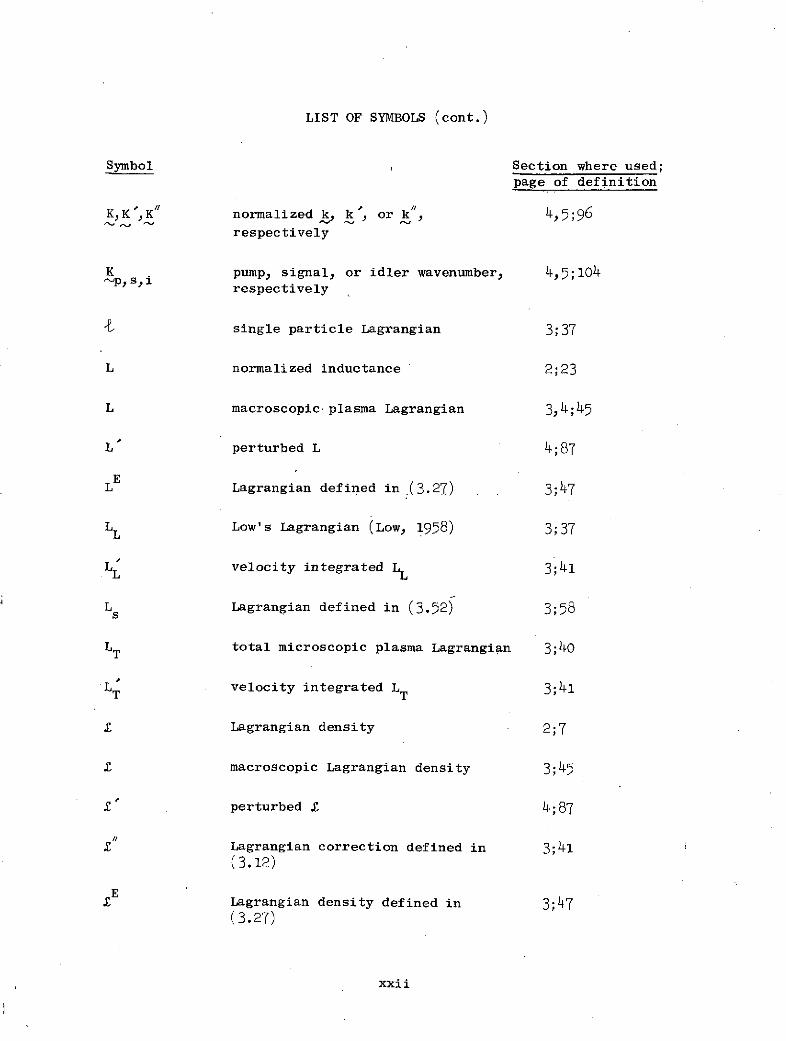
-single particle Lagrangian 3;37
L normalized inductance 2;23
L macroscopic plasma Lagrangian 3,4;45
L perturbed L 4;87
LE Lagrangian defined in (3.27) 3;47
LL Low's Lagrangian (Low, 1958) 3;37
LL velocity integrated LL 3;41
Ls Lagrangian defined in (3.52) 3;58
LT total microscopic plasma Lagrangian 3;40
LT velocity integrated LT 3;41
X Lagrangian density 2;7
£ macroscopic Lagrangian density 3;4r
£ perturbed £ 4;87
iLagrangian correction defined in 3;41(3.12)
IE Lagrangian density defined in 3;47(3.27)
xxii

LIST OF SYMBOLS (cont.)
Symbol Section where used;page of definition
i ith order perturbation expansion 4;93of I (i = 1,2, ... )
.L Lagrangian density of LL 3;37-
£ velocity integrated £L 3;41L L
SNewcomb's Lagrangian density 3;36(Newcomb, 1962)
£ Lagrangian density defined in (3.51) 3;58s
m electron mass 2;26
m particle mass of a species l,3;1
m e, electron or ion mass, respectively 4;96
M total number of dependent variables 2;7
M function defined in (4.66) 4,5;114
M0 constant defined in (4.66) 4,r;114
M function defined in (2.17) 2;121
M , M ,xx xy elements of M 4;99
... , Ms
polarization constant of the sth 4a;99particle species
Tnh function defined in (2.4) 2;8
n arbitrary function of x. 2;12
n perturbation electron density 2;26
xxiii

LIST OF SYMBOLS (cont.)
Symbol Section where used;page of definition
n density of a particle species 1,3;1
n density at A' after virtual 3;47displacement
n density at x after perturbation 4;87
n normalized n 2;26
nO static electron density 2;26
nO initial value of n 3;58
ne,i electron or ion density, respectively 4,5;97
n. ith order nonlocal expansion of n , 4;911 (i = 1,2,...)
nLi ith order local expansion of n', 4;91(i = 1,2,...)
nn neutral density 5;135
N total number of independent variables 2;7
N vth order Bessel function of the 4;116second kind
n function defined in (2.4) 2;8
K/D 4; 100
Pi function defined in (2.43) 2;19apy
Pi function defined in (2.43) 2;19
P perturbation electron pressure 2;26
xxiv
LIST OF SYMBOLS (cont.)
Symbol Section where used;page of definition
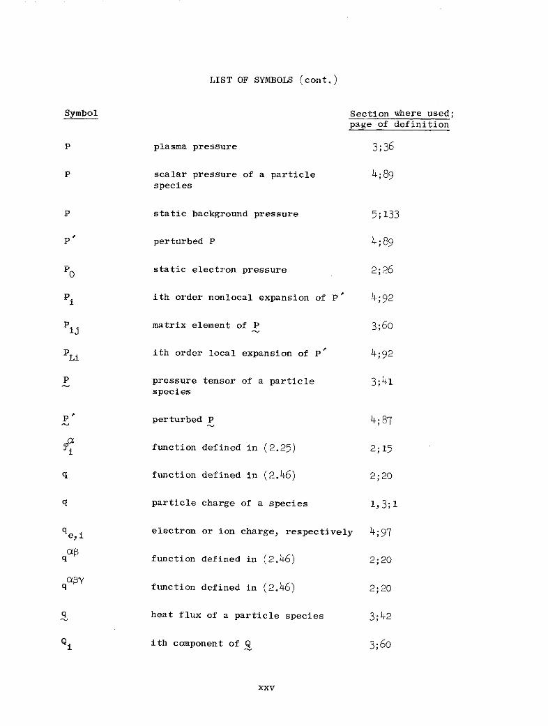
P plasma pressure 3;36
P scalar pressure of a particle 4;89species
P static background pressure 5;133
P perturbed P 4;89
PO static electron pressure 2;26
Pi ith order nonlocal expansion of P' 4;92
Pij matrix element of P 3;60
PLi ith order local expansion of P' 4;92
P pressure tensor of a particle 3;41species
P perturbed P 4;87
function defined in (2.2) 2;15
Sfunction defined in (2.46) 2;20
q particle charge of a species 1,3;1
qei electron or ion charge, respectively 4;97
Sfunction defined in (2.46) 2;20
q function defined in (2.46) 2;20
qheat flux of a particle species 3;42
Qi ith component of Q 3;60
xxv

LIST OF SYMBOLS (cont.)
Symbol Section where used;
page of definition
Q energy transport by heat 3;43conduction
Q function defined in (2.25) 2;15
R normalized resistance 2;23
R function defined in (2.49) 2;22
R. position of the center of AV 3;43
Uf function defined in (2.33) 2;171
S entropy 3;73
S entropy function defined in (3.96) 3;73
SO entropy constant 3;73
S function defined in (2.49) 2;22
t displacement in time 1,2,3;1
tl't 2 limits of integration in time 3;r4
T normalized t according to (2.57) 2;26
T normalized t according to (4.30) 4;96
TO quiescent plasma temperature 4;122
T electron or ion temperature, 5;133respectively
Texp explosive instability period 4;110
T. function defined in (2.49) 2;22
JN kinetic energy contribution to N 3;36
xxvi

LIST OF SYMBOLS (cont.)
Symbol Section where used;page of definition
u constant defined in (5.34) 5;157
u hydromagnetic plasma velocity 3;36
U a th dependent variable 2;7
U. derivative of U with respect to x. 2;71 1
U.1 second derivative of U with respect 2;14to x. and x.
UU group velocity of the U wave 5;1
ix. x- or z-component of ., 4,5;119respectively
A x- or z-component of Us 45;119respectively
K group velocity of the U wave with 4;103wavenumber K
,i pump, signal, or idler wave group 4,5;104velocity, respectively
U 1 . of the U wave 4;104psl ~ psi
v perturbation electron drift velocity 2;26
v normalized v 2;26
v. ith component of v 3;59
vt electron thermal speed 2;26
v particle velocity 1,3;1
v0 initial particle velocity 3;31
xxvii

LIST OF SYMBOLS (cont.)
Symbol Section where used;page of definition
D macroscopic drift velocity of a 3;41particle species
D dv /dt 3;65
vD D at x' after virtual displacement 3;49
vD perturbed v at x 4;87
v. ith order nonlocal expansion of 4;90
D (i = 1,2,...)
Li ith order local expansion of v 4;90i(i = 1,2...)
vR particle random velocity with 3;45respect to v
V normalized voltage 2;23
V spatial volume 3;36
V perturbed V 4;87
V0 initial plasma volume of a 3;37particle species
V new ath dependent variable 2;22
V derivative of V with respect to x. 2;221 1
V ion-acoustic speed 5;139
VA Alfvn speed 5;158
Ve i normalized electron or ion thermal 4,5;96speed, respectively
xxviii

LIST OF SYMBOLS (cont.)
Symbol Section where used;page of definition
V pump wave exciting voltage 5;135
VQM quantum mechanical potential 3;63
Vth threshold of.V 5;135p
macroscopic potential energy density 3;42of a particle species
7 beat condlcition contribution to 1 3;42
" potential energy contribution to £N 3;36
UR random collisional contribution to t 3;42
x one-dimensional displacement in space 2;23
XOi ith component of1o 3;57
x, ith independent variable 2;7
x ith component of x
x. ith component of x 3;57
x.. ax./axoj 3;5711 Oj
x3. dx. ./dt 3;59
x particle position vector 3;31
x macroscopic cell position of a 3;42particle species
0 initial particle position 3;31
p0 initial cell position of a 3;43particle species
xxix

LIST OF SYMBOLS (cont.)
Symbol Section where used;
page of definition
x" macroscopic plasma cell position 3;49after virtual displacement
x perturbed macroscopic plasma cell 4;87position
x 3; 8
x dv/dt 3;65--D
x particle random position with 3;43respect to R
X normalized x according to (2.57) 2;26
X normalized x according to (4.30) 4;119
X normalized x according to (4.30) 4;96
z displacement in the z-direction 4;106
z peak position of Pi(z) 5;135
Z normalized z according to (4.30) 4,5;106
Z0 normalized z0 according to (4.30) 5;138
Z explosive instability length 4;110
(2) Greek Alphabet
a constant defined in (4.89) 4;125
a canonical momentum conjugate to A 3;61
Y adiabatic index for electrons 2;26
Y adiabatic index of a particle 3;89species
xxx

LIST OF SYMBOLS (cont.)
Symbol Section where used;page of definition
y adiabatic index for electrons or 4,5;97ei ions, respectively
Y i Landau damping rate of the 5;141ion-acoustic wave
Fo spatial parametric amplification rate 4,5;106
, 0i idler wave spatial growth constant 4;106
rU normalized temporal damping rate 5;141for the U wave
P normalized collisional damping rate 5;155c
L normalized electron Landau damping 4,5;120rate
r cyclotron resonance damping rate 5;115for whistlers
ps i normalized temporal damping rate of 4,5;112p ' es, or i,, respectively
8 local variation 3;48
8' nonlocal variation 3;48
6.. Kronecker delta 3, 4;581J
8(s-2') delta function in R2 4;98
8(K-K ) delta function in K 4;98
As function defined in (4.41) 4;100
AK departure from synchronism in 4;124wavenumber
xxxi
LIST OF SYMBOLS (cont.)
Symbol Section where used;page of definition
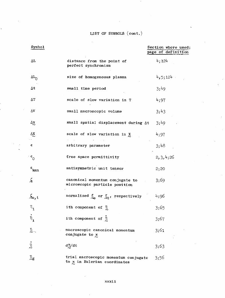
AL distance from the point of 4;124perfect synchronism
AL0 size of homogeneous plasma 4,5;124
At small time period 3;49
AT scale of slow variation in T 4;97
AV small macroscopic volume 3;43
Ax small spatial displacement during At 3;49
AX scale of slow variation in X 4;97
arbitrary parameter 3;48
.0 free space permittivity 2,3,4;26
ekmn antisymmetric unit tensor 2;20
canonical momentum conjugate to 3;69microscopic particle position
,i normalized ~ or i, respectively 4;96
i ith component of 1 3;65
.i3 ith component of 1 3;67
macroscopic canonical momentum 3;61conjugate to x
SdZ/dt 3;63
2 E trial macroscopic momentum conjugate 3;56to x in Eulerian coordinates
xxxii

LIST OF SYMBOLS (cont.)
Symbol Section where used;page of definition
e angle between K and the static ;139magnetic field
e" angle between K' and the static 5;158magnetic field
9" angle between X" and the static 5;152magnetic field
K temporal parametric amplification 4;112rate with wave damping included
0 temporal parametric amplification 4;106rate
KOi idler wave temporal growth constant 4;106
Kth constant defined in (4.63) 4;112
K plasma equivalent permittivity tensor 4;110
AD normalized Debye length 4;96s
AI field-particle interaction contri- 4;101bution to AKK-K"
AT particle thermal contribution to 4;101AKK "K
A(2) K quadratic Lagrangian density in 4;98(K,~) space
Aei(2) electron, ion contribution to 4;98
K'
F(2)AK, electromagnetic field contribution 4;98
to A(2)
AKK" cubic Lagrangian density defined 4;101"~ in (4.46)
xxxiii

LIST OF SYMBOLS (cont.)
Symbol Section where used;page of definition
UVW
AKK K" KK * *, ;104'
O free space permeability 3,4;36
Up normalized spatial damping rate 5;141
of the U wave
normalized spatial damping rate of 4,5;112ps,ip. ,Es, or i., respectively
ix, z i in the X or Z direction, 4,5;119respectively
ss in the X or Z direction, 4,9;119respectively
effective electron-ion and -neutral 2;26momentum transfer collisionfrequency
V constant defined in (4.69) 4;116
v normalized V 2;26
Ve effective electron-ion and -neutral 4;123energy transfer collisionfrequency
v effective electron-neutral momentum 5;133transfer collision frequency
vin effective ion-neutral momentum ';133transfer collision frequency
polarization vector in particle 3;32position
virtual displacement in macroscopic 3;49plasma cell position
xxxiv
LIST OF SYMBOLS (cont.)
Symbol Section where used;page of definition
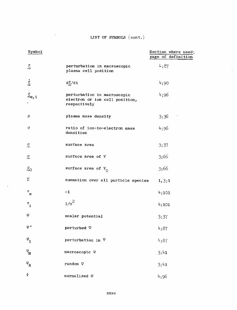
perturbation in macroscopic 4;87plasma cell position
d /dt 4;90
perturbation in macroscopic 4;96electron or ion cell position,respectively
p plasma mass density 3;36
a ratio of ion-to-electron mass 4;96densities
a surface area 3;37
surface area of V 3;66
ZO surface area of V0 3;66
Ssummation over all particle species 1,3;1
e -1 4;101
7i 1/02 4;101
Pscalar potential 3;37
perturbed Y 4;87
CP perturbation in P 4;87
CM macroscopic cp 3;41
PR random CP 3;41
normalized cp 4;96
xxxV

LIST OF SYMBOLS (cont.)
Symbol Section where used;
page of definition
4N equivalent potential defined 4;123in (4.84)
X function defined in (4.69) 4;116
Xlis functions defined in (4.71) 4;117
X 2is functions defined in (4.73) 4;117
Schrdinger wave function 3;63
angle between the static magnetic 4,;119field and 1 or i., respectively
--- -II
w ,c 1 frequencies 4;96
CD electron plasma frequency 2;26
pe electron plasma frequency 4,5;96
normalized w, C,, or w , 4,5;96respectively
"B electron bounce frequency 4,5;120
c c- ,5;100
e c_- 4;100
a. 2 /a 4,5; 1001 c y
si pump, signal, or idler wave 4,r;104frequency, respectively
£c normalized electron cyclotron 4;96frequency
xxxvi

LIST OF SYMBOLS (cont.)
Symbol Section where used;page of definition
(3) Subscripts
o at t = o 3;58
0 static 2;26
1 perturbation 4;87
a acoustic 1;139
A Alfven 5;158
B bounce 4;120
C collisional 5;155
D drift 3;49
e,i of electron or ion, respectively 4;96
i ith order in perturbation amplitude 4;93
H of heat conduction 3;42
i,j ith or jth component of a vector 3;97
i,j,k ... i,j, or kth independent variable 2;10
L Low's (collisionless, Vlasov) 3;37plasma model
L Landau damping 4,5;120
M macroscopic 3;41
n neutral 5;135
N Newcomb's hydromagnetic model 3;36
xxxvii
LIST OF SYMBOLS (cont.)
Symbol Section where used;
page of definition
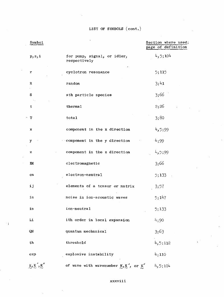
p,si for pump, signal, or idler, 4,5;104respectively
r cyclotron resonance 5;115
R random 3;41
S sth particle species 3;66
t thermal 2;26
T total 3;80
x component in the x direction 4,5;99
y component in the y-direction 4;99
z component in the z direction 4,5;99
EM electromagnetic 3;66
en electron-neutral 5;133
ij elements of a tensor or matrix 3;57
in noise in ion-acoustic waves 5;147
in ion-neutral 5;133
Li ith order in local expansion 4;90
QM quantum mechanical 3;63
th threshold 4,5;112
exp explosive instability 4;110
KK ,K of wave with wavenumber K,K', or K 4 5;104
xxxviii

LIST OF SYMBOLS (cont.)
Symbol Section where used;page of definition
(4) Superscripts
s sth particle species 4;99
E in Eulerian coordinates 3;68
F of electromagnetic field 4;98
U, V, W of the U,V, or W wave 4; 104
a, , y, ... , or Yth dependent variable 2;10
xxxix

ACKNOWLEDGMENTS
I am deeply indebted to my research advisor, Professor Frederick W.
Crawford, for his patient guidance throughout this work and for his
proficient help in organizing the thesis. His advices have profoundly
influenced my view of plasma physics.
I also would like to express my sincere appreciation to Dr.
Kenneth J. Harker for making available numerous hours of discussion
during my study at Stanford and for making constructive criticism in
preparing the thesis.
I am grateful to Professor Peter A. Sturrock for reading and commenting
on the dissertation, and to Professor Oscar Buneman for his beneficial
commentary on computer applications of Lagrangian formulations. Thanks
are also due to Dr. Hongjin Kim for many stimulating discussion sessions
and for verifying the derivations. Numerous fruitful conversations with
Mr. David M. Sears, Dr. Dragan Ilic, and Dr. James J. Galloway are also
acknowledged with pleasure.
I want to thank Evelyn Mitchell, who expertly and cheerfully typed
and retyped this manuscript, and to thank Jane Johnston and Joanne Russell,
who have offered efficient assistance during my study at the Institute
for Plasma Research.
Finally, my deepest gratitude belongs to my wife San-San for her
understanding and encouragement during the entire period of my graduate
work, to my father for his instruction, and to God for His provisions.
xl
1. INTRODUCTION
In theoretical descriptions of plasmas, three approximate models
are commonly employed. These are the cold, .the microscopic, and the
macroscopic plasma models, all of which use Maxwell's equations. To
complete the system of equations, the cold plasma model uses Newton's
force law,
dv (1.1)m d= q(E vX B) ,(1.1)
where E and B are the electric and magnetic fields, and v, m. and
q are the particle velocity, mass, and charge of a species. The
plasma is then regarded as consisting of interpenetrating cold fluids
with charge and current densities, E qn and Z qnv, respectively, where C
sums over all particle species, and n is the particle number density.
The microscopic plasma model uses Newton's force law in (1.1) for each
particle, and the Boltzmann-Vlasov equation (Clemmow and Dougherty, 1969)
f dv-+ v v + * V f = , (1.2)
t + dt v
where f(x,v,t) is the Boltzmann distribution function for each particle
species. The expressions for charge and current densities now become
E qffdv and E qffvdv, respectively. The plasma is regarded as a system
of charged particles evolving under the influence of their own electro-
magnetic fields, and externally applied fields (if any). In principle,
complete solutions to the particle force law for all particles will auto-
matically generate the solution of f(xv,t) because (1.2) is a statement
1

of particle conservation along the particle trajectories in a six-
dimensional phase space (xv). When it is not necessary to obtain the
particle trajectories, solutions of f(x,,t) are obtained by use of
(1.2) together with Maxwell's equations.
The macroscopic plasma model uses velocity moments of the Boltzmann-
Vlasov equation (1.2). Examples of these equations are expressed by
(3.29) and (3.46). The charge and current densities are now written as
C qn and Z qn , where zD is the drift velocity, i.e. the averaged
local velocity of a particle species [see (3.13)]. Here, the plasma is
approximated in terms of localized variables such as density, drift
velocity, pressure, and heat flux. In terms of degree of approximation,
the macroscopic model falls between the other two models.
The appropriate Lagrangians for the cold plasma model (Galloway and
Crawford, 1970) and the microscopic plasma model (Low, 1958) are already
well-known. However, the Lagrangian for the macroscopic plasma model,
that corresponds to Maxwell's equations and the moments of the Boltzmann-
Vlasov equation, has not been established. The gap will be filled in
this thesis.
The interests in developing this variational principle stem from
the fact that current theoretical investigations in nonlinear wave-wave
and wave-particle interaction properties of homogeneous plasmas, and in
linear properties of inhomogeneous plasmas, are at the limit of analytic
tractability. While a suitable variational principle does not provide
new fundamental laws, it leads to a relatively concise formulation and
easy manipulation for these otherwise difficult problems.
To obtain the suitable macroscopic Lagrangian, the first problem that
arises is the inverse problem of the calculus of variations, i.e. the
2
derivation of Lagrangians from arbitrary equations. This mathematical
approach will be examined in Section 2 in contrast to the approach via
energy considerations commonly used for physical problems. From this
general point of view, it will be shown that energy dissipation effects
can be included in variational (minimal) principles,in general, and the
results will be demonstrated with examples.
The approach of the inverse problem treats all dependent variables
as generalized variables. The plasma variational principle to be presented
in Section 3 will treat only the macroscopic plasma cell position and the
electromagnetic potentials as generalized variables. This type of formula-
tion for a system of discrete charged particles, was described in a
relativistically covariant form by Landau and Lifschitz (1969), and
in the non-relativistic form by Goldstein (1950). Extensions of these
Lagrangian densities to the microscopic plasma model to include a velocity-
distributed system of particles,.have been proposed by Sturrock (1958a)
and Low (1958). Based on Low's Lagrangia and using energy considerations,
we shall obtain the corresponding Lagrangian and Hamiltonian for the
macroscopic plasma model, with the effects of viscosity, heat conduction,
and elastic collisions takeh into account.
In applications of Lagrangians to problems involving homogeneous
plasmas, there has been progress in the areas of linear waves (Kim, 1972),
nonlinear three-wave interactions (Galloway and Crawford, 1970), wave-
background interactions (Dewar, 1970), wave kinetic equations (Suramlishvili,
1964 and 1965; Galloway, 1972), higher order nonlinear wave processes
(Dewar, 1972; Dysthe, 1974), and statistical analysis of plasma turbulence
(Kim and Wilhelm, 1972). For problems in inhomogeneous plasmas, results
3
have been presented in the area of energy principles (Newcomb, 1962), and
in the use of the Rayleigh-Ritz procedure to obtain approximate solutions
(Dorman, 1969). As compared with other branches of physics, these cases
comprise a disproportionately small fraction of the theoretical effort
in plasma physics.
In this work, the new macroscopic Lagrangian will be used in two
ways. In Section 4 we shall be concerned with the general description
of nonlinear three-wave interactions in a homogeneous plasma by use of
the averaged Lagrangian technique (Whitham, 196'). These results will
be specialized in Section 5 to parametric amplification of ion-acoustic
waves to make quantitative comparisons with available experimental data.
The second application of the Lagrangian will be presented in Appendix BY
where the Rayleigh-Ritz procedure is applied to obtain approximate solu-
tions for electrostatic resonances in a low pressure positive column. It
will be shown that the results compare favorably with available experimen-
tal data and conventional numerical calculations by others (Parker, Nickel,
and Gould, 1964).
Some conclusions are drawn in Section 6, where new contributions and
future extensions of this research are briefly discussed.
4
2. INVERSE PROBLEM OF THE CALCULUS OF VARIATIONS
2.1 Introduction
In the calculus of variations Hamilton's principle is applied to
the integral of a given Lagrangian density, often referred to. as the
action integral, to obtain the Euler-Lagrange equations extremizing the
action integral (see for example, Courant and Hilbert, 1966). The
inverse problem of the calculus of variations is to find the conditions
that arbitrary differential equations must satisfy to be the Euler-
Lagrange equations of a certain Lagrangian density, and to determine
an appropriate Lagrangian density from the given differential equations.
The term 'Lagrangian density' as used here will include cases with
multiple independent variables. Recent developments of a method of
studying weakly nonlinearwave propagation in distributed systems makes
the inverse problem for a system of partial differential equations of
particular interest (Whitham, 1965; Galloway and Crawford, 1970; see
Chapter 4). A general approach is required to obtain appropriate Lagran-
gian densities for systems of equations including effects of energy loss
due to .heat flow, viscosity, and collisions.
The inverse problem of the calculus of variations attracted
attention over a century ago, when Jacobi (1837) examined the character-
istic properties of an ordinary Euler-Lagrange differential equation of
second order (Kiirschak, 1906; Akhiezer, 1962). More involved problems
have since been studied. Such work includes that by LaPaz (1930), who
treated the case of one dependent variable in many independent variables
using the necessary property of self-adjointness of the Euler-Lagrange
equation. Douglas (1941) has studied the case of many dependent variables

in one independent variable, by considering the characteristic forms of
the coefficients in a system of Euler-Lagrange equations. Van der Vaart
(1969) has applied the results of Douglas (1941) to a system of ordinary
linear differential equations of second order. A survey of the litera-
ture on this approach to the inverse problem may be found in the book
by Funk (1970).
The general case of many dependent and independent variables has
been considered by Vainberg (1964). By treating the dependent variables
as points in a coordinate system of functions, the invariance of an action
integral under the variation of the functions is shown to be analogous
to the invariance of a potential under the variation of the path of inte-
gration (Tonti, 1969a). This analogy has led to definition of poten-
tiality conditions for the operators of the system of equations. For
differential equations, these potentiality conditions are then the necessary
and sufficient conditions for solutions of the inverse problem of the
calculus of variations (Tonti, 1969b).
The treatment to be-presented in Sections 2.2 and 2.3 will be con-
fined to quasilinear differential systems of first and second order,
respectively. We shall emphasize special forms of the Euler-Lagrange
differential system, following the approach used by Douglas (1941), while
generalizing to the case of partial differential equations. Since we
are looking for some scheme that generates a Lagrangian density, the
conditions for the given equations to be Euler-Lagrange equations will
be established in such a way that, once satisfied by the differential
equations, an explicit Lagrangian will be derivable. The cases of linear
and weakly nonlinear differential equations are treated as examples in
Sections 2.2.3 and 2.3.3, respectively.
6

In supplement to these conditions, the nonuniqueness in the form of
the given differential system requires discussion: there are operations,
such as multiplication of the system by some matrix expressions (Davis, 1929),
and changes of the dependent variables, that can convert apparently non-
Euler-Lagrange equations to equivalent Euler-Lagrange equations. In
Section 2.4, we shall discuss one of these techniques, differential
transformation of the dependent variables. As examples, we derive
appropriate Lagrangian densities for a resistive transmission line, and
for a warm collisional plasma in Sections 2.4.2 and 2.4.3, respectively.
2.2 First Order Differential Equations
A system of first order quasilinear differential equations has the
general form,
C U + D = 0 (i=l, ... , ; , = 1, ... , M) , (2.1)
where the coefficients C. and D are explicit expressions in indepen-1
dent variables x. and dependent variables Up, and U is written for1 1
the derivative U /3x i. Repeated indices of i (or j,k, ... etc.) are
summed over the N independent variables; repeated indices of a (or
., y, ... etc.) are summed over the M dependent variables. We see that,
in general, the numbers of the CT and Da are MN and M
respectively.
The inverse problem of the calculus of variations aims at deriving
a Lagrangian density, £ [= £(U~, U, xi)], that gives (2.1) as the set
of Euler-Lagrange equations obtained by extremizing the action integral,
I = dNx £(U, U, xi) , (2.2)
7
through variations of the dependent variables, U . For an arbitrary
i (UI, U~, xi), the Euler-Lagrange equations take the form,
dx alO N, M) (2.3)
where d/dx. operates on both the explicit and the implicit x -
dependences through Ui (x.) and U (x.).
Equation (2.3) is a highly specialized form of (2.1): the coefficients
Ci andu D are functions only of the derivatives of I (U, u xi).
The necessary conditions for (2.1) to be a set of Euler-Lagrange equations
will be obtained in Section 2.2.1 by elimination of X (uC, Uf, x.) from
the expressions for q and D . More important, however, are the suffi-
cient conditions on CT and DP so that a corresponding £ (UI, Ui, xi)
exists. In Section 2.2.2, we shall establish conditions which will enable
us to solve the expressions of Co and D for S (U, U, xi).1 1
2.2.1 Necessary Conditions
In view of (2.3), £ must be linear in the U6 to give a set of1
Euler-Lagrange equations of the form (2.1). We write
c= xU0 +v (2.4)
where M [=a (Ux )] and [= (U,xi)] are functions of UC and
xi' The Euler-Lagrange equations of this Lagrangian density with respect
to U a then become
S-+- - =O . (2.5. U 1 x i au
8

Comparing (2.1) and (2.5) gives,
3ni i _ 6)0 6C i i D ' i a (2.6)1 B U axi U
The C. and D must satisfy the following equations, obtained by1
eliminating the T and R from (2.6),1
CT + CC = 0 , , -E- + + - = 0 . (2.7)1 1 axi Ip 2mU 6U U UP
2.2.2 Sufficient Conditions
Given C43(U',x.) and D(UP,x.), we require conditions sufficient
to guarantee that (2.6) can be solved for the i 1 and ) in terms of
the Up and x.. Note that the uniqueness of solutions is not required.1
The first equation of (2.6) represents at most M2N equations for
the MN unknowns Ml , with Up as independent variables. For l to1 1
exist, (2.7) must be satisfied. In particular, C! = _C C, so that
the number of distinct equations covered by the first equation of (2.6)
is reduced to MN(M-1)/2. These can be divided into N independent
groups of M(M-1)/2 equations for each i. Consider in each of these
groups the subset of equations relating Ma i and '. If we
assume a form for T R, we may then use the first expression in (2.6),
which yields
a c , -- , (2.8)
9
to solve for T. and 1Y, subject to the constraint that the particular1 i
solutions-of T. and m. must satisfy1 1
i 1 (2.9)
This self-consistency condition requires that C , C and C satisfy
the final relation of (2.7).
As a digression, it is of interest to note that this self-consistency
condition is analogous to the well-known condition that magnetic fields
are source-free. For the magnetic field, B, and the corresponding
vector potential, A, we have
V. B = 0~ B = VX A (2.10)
The analogy follows by taking a = 1, P = 2,y = 3, and
B = I 3C 3,C 2 A = M2~m M o , = -' a 3u iU2' iu 3
(2.11)
The foregoing argument is valid for any triplet from the set Mac.
Therefore, with Inu arbitrarily chosen, and the final expression of (2.7)
satisfied, we can always use the first relation of (2.6) to solve for
i13ui', etc. Having obtained this set of particular solutions, they can
be substituted in the second expression of (2.6), together with the
given DP, to obtain M equations for the single unknown function (U P).
A solution for n exists if we have
10 U ) U (2.12)
10
Use of (2.6) indicates that this condition implies that the D must be
related according to (2.7).
The consistency relation of (2.7) for triplets such as CT, CY ,
CYC6 reduces the number of independent equations in (2.6) from M(M-I)/2i
to (M-l) for each i. This follows since use of the equations,
1 2M2 1 312 1 13
C 1 2 1 1 1 3 1 , (2.13)U U U U
in the final expression of (2.7) will result in
C23 = - + A(U2 ,U3 ) (2.14)i 6U3 2)U2
where A(U2;U 3 ) is the constant of integration. Since nR2 and JR3i 1
also contain arbitrary functions of U2 and U 3 , because of (2.13),
it is always possible to adjust them to make L(U 2,U3) = 0. Symbolically,
we can express the result that (2.14) follows from (2.13) as
12, 13 - 23,
12, 13, 14 - 23, 24, 34,
12, 13, 14, 1M - 23, 24, ... , (M-I)M
Thus, by imposition of the third condition of (2.7), the first expres-
sion of (2.6) is reduced to only M-1 independent equations for each i.
By choosing 1 arbitrarily, M (p > 1) can then be obtained consis-
tently by use of (2.6).
11

It is now clear that the relations expressed by (2.7) are the necessary
and sufficient conditions for (2.1) to be a set of Euler-Lagrange equations
of a Lagrangian density of the form given in (2.4). When expressions
for C. and Da satisfying these conditions are given, the procedure1
for deriving the corresponding Lagrangian density will involve only
direct integrations. It should be noted that since 31 is arbitrary,1
the set of 31 and the function R are not unique. In addition to the1
freedom in choosing , the set of a and the function n are deter-
mined only to within arbitrary functions of the x..
2.2.3 Linear Differential Equations
As an exercise, we shall derive a Lagrangian density for a system
of first order linear differential equations for which
C = c (x i ) , D = d (xi)U + e (xi) 21
The sufficient conditions of (2.7) then reduce to
acapcCI = d - dPaC (2.16)
where the final relation of (2.7) has dropped out. We shall choose a1
to be the form, MTU where, by (2.6), the MT are related according
to
c = M - MTa (2.17)1 i i
For convenience, we shall impose the condition MC = -Mp..X 1
With the assumed form of 3l, we obtain by use of (2.6)
U - e(2.18)
12

Accordingly, ) assumes the form,
S= N U - eAC + n(x) , N- d )= N . (2.19)
Combining these results into (2.4) gives the Lagrangian density
1 = ciUiU + 2d U U - eU + n , (2.20)
where n is an arbitrary function of the x..1
2.3 Second Order Differential Equations
A system of second order quasilinear differential equations can
always be transformed into a first order differential system by treating
the derivatives of the dependent variables as new dependent variables
(Courant and Hilbert, 1966). However, this approach to the inverse
problem is unsatisfactory for plasma problems because the introduction
of new dependent variables is equivalent to introducing artificial
degrees of freedom. Also, if we leave the number of degrees of
freedom unchanged, the Lagrangian density for second order differential
equations describing physical systems generally has a corresponding
Hamiltonian density, 3C. Conditions sufficient for the existence of a
Lagrangian density, J, will then also guarantee the existence of (,
and allow it to be used in such applications as evaluating nonlinear wave
coupling coefficients (Sturrock, 1960a; Harker) 1970).
For purposes of example, the system of quasilinear second order
differential equations will be assumed to have the form
13

A U + B = 0 (i = 1, ... , N; ,B = 1, ... , M) , (2.21)
where Ua is the set of dependent variables; the coefficients A andij
B are functions of U , Ut, and x., and U. and U . denote theS1 i 13
first and second derivatives of U , respectively. Since UC. = U.,
the matrix A. can be assumed symmetric in the indices i and jij
without loss of generality.
2.3.1 Necessary Conditions
Equation (2.3) may be written
2 2 2a U. +6 U -0 . (2.22)6U aU P 6vBU i arU 3x. 6U
Comparing with (2.21) gives the necessary conditions for that system to
be the set of Euler-Lagrange equations of £ as
2AO 2 + , B = U + (2.23)1) 6UBU P 6uB u 1 UTP U ax 6U,1 j j 1 1
Eliminating £ allows us to express these conditions in the form
j + jk ki + ki
k J
+. . 62i + UB6B- A+A = A. , + - 2 + Uiij ij U iUt bYxj U
1 1
( + a 73 6 0 +A B + 1 1 _ B + _2B (2.24)2)x k k Ua aUp bu Ij a U 2 trf kUc U U 6U
14
14

2.3.2 Sufficient Conditions
We can assume the general form of the Lagrangian density as
S= p(u,u,xj) + ya(UP,x.)U + Q(Uaxi) (2.25)
where 9 is responsible for A ij. Then it follows from the first rela-
tion of (2.23) that
2A = 2 + 2 (2.26)
where only the set (U$J are treated as independent variables. By
interchanging a and B, we see that this differential equation can
be solved only when A = A.., which is the second relation of (2.24).ij ji31
Equation (2.26) constitutes MN(M+l)(N+i)/4 linear differential
equations to be solved for P. For p to exist, consistency among the
third order partial derivatives is required, i.e.
(2.27)
This implies that the first condition of (2.24),must be satisfied.
In the cases where either a = B or i = j, 9 can be obtained
by simple integration of (2.26). When both a P B and i 4 j, (2.26)
becomes an ultrahyperbolic differential equation with constant coeffi-
cients (Koshlyakov, Smirnov, and Gliner, 1964). Its particular solutions
can be obtained by Fourier transforms (Koshlyakov, Smirnov, and Gliner,
(1964). The general solution of 9 should include that of the homo-
geneous equation,
15
+ a = 0 (2.28)
which can be solved by separation of variables (see Appendix A). We shall
show below that this nonuniqueness in will be restricted by other
sufficient conditions.
From the second expression of (2.23) and (2.25), we obtain,
U. + - U - b a- + B (2.29)
\BU Bel - OJi bU ' ua BU Bixi v U
Since (2.29) is an identity in U, U , and x., the right-hand side
must be linear in U. Taking the derivative with respect to Ui, yields
4 aB 2 2 2+ U + a V - b + (2-30)
the left-hand side of which is antisymmetric in a and P. The third
expression in (2.24) guarantees that the right-hand side is also anti-
symmetric in a and P. However, the fourth expression, which shows that
(2.31) is symmetric in i and j, is not sufficient to establish that
the right-hand side of (2.30) is independent of U . This requirement1
can be obtained by differentiating (2.30) with respect to U,
+ U8 a 6 a 2 + a3 + a 2 (t231)
R bxk k a aup bUU au 06b aU' bU U B U UC cB U aUpb
This is more restrictive than the third necessary condition, and represents
limitations on in addition to the fourth.
16

Additional conditions from (2.30) for P. to exist arei
S+ . + - 0 , (2.32)
analogous to the last expression of (2.8), where Q is defined by1
-+j al. a (2.33)
The solution of (2.30) enjoys one arbitrary choice of , just as the
solutions of the first expression of (2.6) for 3n, for each i. But
if (2.29) is to give a consistent solution for 0, additional conditions
restricting the set of i then follow from (2.29), from the requirement
that
a-ua ( ) fu ua) (2.34)
analogous to (2.12). We have
+ U a + + eU Y !Uu)(611 abaau auauc au au ' 1uY au 6uC"
(2.35)
In summary, sufficient conditions for (2.21) to represent a set of
Euler-Lagrange equations of a Lagrangian density, I, of the form (2.25)
are as follows: for a solution of (2.26) for to exist, AT must1ij
satisfy the first two conditions of (2.24); for a solution of (2.30) for
P? to exist, g must be further restricted by (2.31) and (2.32), while
A. and B must satisfy the third condition of (2.24); for a solutionj1
17

of (2.29) for 0 to exist, T, p, and Ba must be restricted by (2.35).
These conditionsas well as those of Section 2.2.2 for first order equa-
tions agree with the general forms obtained by Tonti (1969b) by poten-
tiality analysis of differential operators in function space (Vainberg,
1964; Tonti, 1969a).
2.3.3 Nonlinear Differential Equations of the Second Rank
As a demonstration of the foregoing results, sufficient conditions,
and the corresponding Lagrangian density, will be obtained for the
differential system
A.. = a°l + aTY U + a1j ij ij ijk k '
B b + b U + b UU+ b.U + b U' + + UbY boUU. (2.36)1 1 ij 1 j
o ~ aThe coefficients, a , etc. and b , etc., are functions of xi; the
a. are symmetric in i and j, the bC y in p and y, and theij
bO . in (p,i) and (y,j). With the coefficients of (2.36), the equa-1j
tions of (2.21) are nonlinear and of the second rank because of the
presence of a. , aY bO43 bTY and b0"ij ijk' i ij
Substituting (2.36) into (2.24) yields for the a0 , etc.,ij .
ao= a aO=Y a( , a?.Y = a OYj 13 ij 1 ij 1j ijk Ljk
aC + a o Y ap y + aYC4 (2.37)ijk jki kij kij
and for the b , etc.,
18

bi + b = 2 ( bP- + b) = 2/ i,
aybOY + bo- ay ijk1b + bj a1 + (2.38)ij 1j ij x k
We can now assume the general form for 2 as
+)TYUCVupuy +1 (aT a Y Y a u% , (2.39)ijk i j k 2 j (2.39)
and choose to impose
S Y (2.40)ijk = jik ikj (2.)
The requirement of (2.31) reduces to
xk ij j - (2.41)
while (2.32) becomes
bO + b Ya + b4' = a a + a . (2.42)"- j\ ij ij ij
Using (2.30) we find that ap takes the form
1 = pU + pUU' , (2.43)
where p. and pi are to be obtained from the differential relations,
pT p b 13 pj y po 4 1. (2.44)xx (2.)
19

The conditions of (2.35) reduce to
i 1 7 , (2.45)bC - - aB x x(
without further restricting the choices of p. and p
The general form of Q is
0 = -bU~ + qC43UU + qO4YUU + q(xi) , (2.46)
where, according to (2.29),
-qb apq- q CY _ 1 , (2.47)
and q(xi) is arbitrary.
We find that the Y are determined from (2.41) only to within anijk
arbitrary curl tensor, e bd9 /x , where e is the antisymmetrickmn 13 n m kmn
unit tensor. According to (2.44) the p. and p are both deter-1 1
mined only to within an arbitrary tensor symmetric in a and 8.
In the special case that the set of differential equations expressed
by (2.21) are linear, the relevant sufficient conditions reduce to
aT = a C b0 + b = 2 j) b0 - bB (3 a ijij 13 1 i - axx 1 ax
(2.48)
These are equivalent to those used by van der Vaart (1967), who con-
sidered the case N = 1 [Equation (16) by van der Vaart (1967)].
20

2.4 Differential Transformations
In Sections 2.2 and 2.3, we assumed that the QCth equation of the
differential systems represented by (2.1) and (2.21) is an Euler-Lagrange
equation with respect to variation of U0. Now these sets of equations
are transformable, for example by change of variables, to equivalent
sets which no longer satisfy the sufficiency conditions. Solution of
the inverse problem of the calculus of variations is consequently less
restrictive than is suggested by the sufficiency conditions: it may be
possible to convert seemingly non-Euler-Lagrange equations to Euler-
Lagrange equation form by use of appropriate transformations. The
problem this poses is how to recognize when such transformation is
possible. Here we shall comment briefly on the transformations likely
to be involved. We cannot provide a general solution.
Among the range of possible transformations, those retaining the
number of dependent variables unchanged include: (a) matrix transformation
of the dependent variables; (b) matrix transformation of the differential
equations, by use of integration factors, leaving the dependent variables
unchanged (Davis, 1929); and (c) differential transformation that raises
the order of the differential equations. For a self-consistent system
of M differential equations,Method (a) involves M2 functions of x.
as the elements of the transformation matrix; Method (b) involves M2
functions of x. as matrix elements, the dependent variables, and
perhaps their first derivatives, while Method (c) involves only M
functions of x., the new dependent variables, and their derivatives.
In each of these cases, the number of functions at our disposal in
general falls short of the number of sufficient conditions to be applied.
21

Consequently, we cannot expect that these methods will always be success-
ful in transforming non-Euler-Lagrange equations to Euler-Lagrange equations.
Despite their inability to guarantee successful transformation,
methods (a)-(c) are of interest in dealing with equations of forms, such
as those occurring in some physical and engineering problems, where the
number of sufficient conditions is reduced. Well-known examples can be
readily found in the cases of replacing electromagnetic field variables
by potential variables (Goldstein, 1950), and velocity variables by
Clebsch variables (Lamb, 1930), before the Lagrangian densities can be
obtained. To illustrate their use here, we shall apply a linear differen-
tial transformation to convert a first order linear non-Euler-Lagrange
system to a second order Euler-Lagrange system in Section 2.4.1. Using
the sufficiency conditions obtained in Section 2.3.3, we shall then
determine the maximum number of dependent and independent variables for
a successful transformation to be possible. As examples, a resistive
transmission line, and a warm collisional plasma, will be studied in
Sections 2.4.2 and 2.4.3, respectively.
2.4.1 Differential Transformation of Linear Differential Equations
Under the linear transformation,
uv = T (x.)V + SI (x.)V + R(x.i ) , (2.49)1 31 1
the first order linear differential equations of (2.1) and (2.15)
become second order equations, with coefficients of the form (2.36)
given by
22

a i Tj + cT. b. = c+ d + SIJ j 1 1 j i J 1
b = ciL d S , b =c dRB + e . (2.50)
The sufficiency conditions imposed on these coefficients by (2.48)
constitute MN(M-1)(N+l)/4+MN(M+1)/2+M(M-1)/2 conditions to be
satisfied by the M 2(N+l) unknown functions, T and SP. The1
number of unknowns will consequently be no less than that of the
conditions only when
M(M-1)(N+I)(N-2) 4M . (2.51)
When (2.51) is satisfied, the equations obtained by substituting
(2.50) into (2.48) are in general solvable for the T, SP, and
for the given coefficients c , d , and e . The resulting second
order differential equations will automatically become Euler-Lagrange
equations, with the corresponding Lagrangian density derivable using
the results of Section 2.3.3.
2.4.2 Resistive Transmission Line
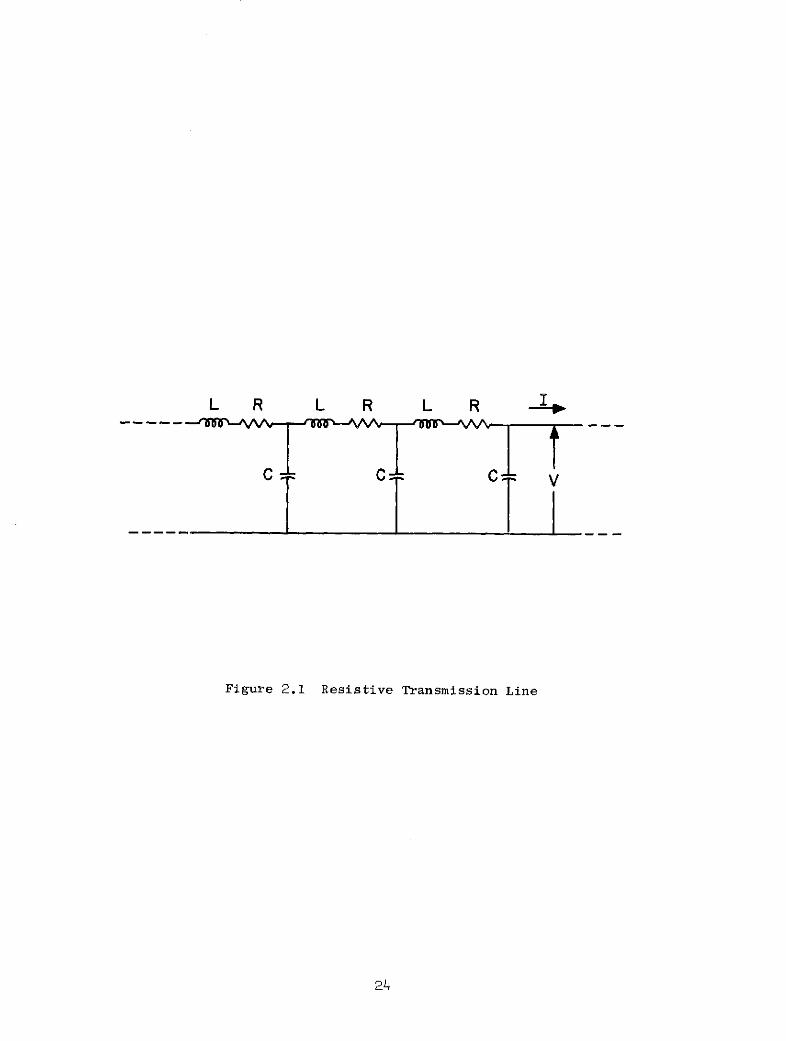
The first order equations for a linear resistive transmission line,
as shown in figure 2.1, take the form,
I + V cvI v- + C = 0 L b + - + RI = 0 (2.r2)ax at at 6x
where I, V, C, L, and R denote the normalized current, voltage,
distributed capacitance, inductance, and resistance, respectively.
According to (2.16), (2.52) is not in Euler-Lagrange equation form.
23
L R L R L R
Figure 2.1 Resistive Transmission Line
24
With [I,V] = [U ,U2] and If,g) = [V ,V2 , the procedure outlined in
Section 2.4.1 may be followed to give
Lv ,x (2.53)
as an appropriate transformation. The corresponding Lagrangian density
is obtained, through the use of (2.25), (2.39), (2.43), (2.44), (2.46),
and (2.48), in the form,
= + 2 + L bx ) + CL _-
S2 VF) ax ax a aat 0
SL af 2 / g 2+ L c + + + 2 - L _ax ( t at 2 I t )t at (t
RC [gibf +f) lg +g C 2 22 a at x at I
The Euler-Lagrange equations of (2.54) can be shown to agree with the
result of using (2.53) in (2.52). Because the number of sufficient con-
ditions is less than the number of transformation coefficients, Ti
and S , (2.54) is but one example among an unlimited number of appro-
priate Lagrangian densities.
2.4.3 Warm Collisional Plasma
For small one-dimensional perturbations in a plasma with a homogeneous
immobile neutralizing positive ion background, the macroscopic equations
25
E en an av avS+ -- = 0 -- + n O ,0 m -- + mvv + YP n + eE = 0ax a0 t o0 x t x'
(25)
where m and e are the electron mass and charge; no and PO are the
quiescent electron density and pressure; v is the effective electron-
ion and electron-neutral momentum transfer collision frequency; y is the
adiabatic index, and cO is the permittivity of free space. The pressure
anterm, yPo a nO' results from assuming an adiabatic equation of state
for the electrons,
(P+P)(nO+n)-Y = POn0 Y (2.56)
In (2.55), the dependent variables are the electric field, E, the
electron density perturbation, n. and the electron drift velocity, v.
Application of (2.16) indicates that these equations are not in Euler-
Lagrange equation form. They satisfy (2.51), however, so that the
differential transformation defined in Section 2.4.1 can be used. To
reduce apparent complexity, it is helpful to rewrite (2.55) in terms of
normalized variables, defined by
- eE - n - vE = n vmvt p n vt
M xtp 0 t
Tt v- (2.57)P X
wrt Pv[emP
where vt [= (PO/m)1 / 2 ] and [= (noe2/m) 1/2] are the electron
thermal velocity and plasma frequency, respectively. We then have, in
place of (2.55),
26

-E an av ay an -S+ + 0 , + v v + Y- + E 0 (2.58)x nT ax BT x
From (2.48) - (2.50), and (2.58), it can be shown that are appropriate
transformation,
E C11 C12 C13 f
S C C C 23
L 31 C32 C33 j hj
should have the following elements:
C -- +-a C - c - a11 ax 12 CX a '
C -ya +c b -vc C =c13 X T 21 C '
C d C d c v d C -a22 N ' 23 BT ' 31 X Y
C 3 2 c e ax--+ a (2.60)32 y ' C33 -
where a, b, c, d, and e are arbitrary constants, except that they should
make (2.59) a reversible transformation.
The corresponding Lagrangian density, obtained through using (2.25),
(2.39), (2.43), (2.46), and (2.48), may be expressed in terms of f, g,
and h as,
27

bf 2 +- f ag + iag f h Ye ah2Xax X X I ax 2 aX
/ \2 - 2e h ag d hf
+ + + (d+e)2Y BT WT a ax aT ax aT e x aT
+(b + c - e) -h f + (c + v d) _- g + g+a - hbX ax Y aT aT
+ f- a fh + + V~+ h (2.61)-
The Euler-Lagrange equations of (2.61) can be shown to agree with the
result of using (2.59) and (2.60) in (2.58).
2.5 Discussion
In this section, we have considered the inverse problem of the cal-
culus of variations for systems of first and second order quasilinear
partial differential equations. The approach has been to compare the
form of the Euler-Lagrange equations with that of an arbitrarily chosen
set of equations. The resulting sufficiency conditions agree with
general results obtained previously by the more abstract method of imposing
conditions of potentiality of operators in a function space (Vainberg,
1964; Tonti, 1969). By restricting ourselves to equations of quasilinear
form, we were able to determine the Lagrangian density explicitly, if the
sufficient conditions are satisfied by the given set of differential
equations. As examples, the results were applied to systems of first
order linear equations, and second order nonlinear equations.
The explicit formulation described here has led to some success in
using differential transformations to convert non-Euler-Lagrange equations
to Euler-Lagrange equation form by changing the dependent variables. The
28
examples on the resistive transmission line and warm collisional plasma
served to show their importance. This operation, together with the
other transformation techniques discussed in Section 2.4, constitute
powerful mathematical ways to define appropriate generalized (dependent)
variables in a given inverse problem. This is complementary to the
procedure of choosing suitable 'geometric' and 'force' variables in
physical variational problems, described by Penfield and Haus (1967).
Our discussion of transformation techniques suggests some significant
problems for further study in the inverse problem of the calculus of
variations. For instance, recognition of equivalent systems of formally
different differential equations becomes important if the area of appli-
cation of the inverse problem is to be enlarged.
Although the mathematical approach is rigorous, the need to choose
appropriate generalized variables, and to rewrite the equations in Euler-
Lagrange equation form, reduces the practical value of our approach to
the inverse problem in those physical situations in which intuitive energy
considerations can be readily used to guess at, and establish appropriate
Lagrangian densities. The latter approach relies on the experience that
a physical system with well-defined energy can be described in terms
of Hamilton's variational principle. The trial procedure then involves
assigning generalized variables, according to the number of degrees of
freedom, before guessing a Lagrangian density that includes various
forms of kinetic and potential energies. The trial Lagrangian is then
checked by the relatively simple process of applying Hamilton's principle
to produce Euler-Lagrange equations that are the correct equations of the
problem. A small number of trial-and-error exercises may then result in
a suitable Lagrangian density.
29
In anticipation of the Lagrangian applications to plasma physics,
to be discussed in Section 3, we may point out two other problems. The
first concerns the explicit distinction between dependent and indepen-
dent variables generally assumed in the inverse problem; the variation
principle established in Section 3 relies on an unorthodox arrangement
which we term the 'dual role' of the variables. This dual role can be
understood to be some implicit dependence, in the form x[y(z)], with
both x and y assuming the role of generalized variables. The exten-
sion of the present results to incorporate this dual role is a problem
that we have not had time to study in detail.
The second problem is related to the so-called 'Lagrange (or Bolza)
problem' (Rund, 1966; Bliss, 1946). This deals with the variation
principles whose solutions are to be determined under subsidiary constraints.
This type of problem immediately introduces serious practical difficulties
into the corresponding inverse problem, since there is no mathematical
rule to determine which of the given differential equations are to be
treated as constraint equations. In the corresponding physical problem,
however, no such difficulty arises once the degrees of freedom are
determined.
30

3. LAGRANGIAN AND HAMILTONIAN DENSITIES FOR PLASMAS
3.1 Introduction
In this section, appropriate Lagrangian and Hamiltonian densities
will be established for the macroscopic model, in which the plasma is
described by Maxwell's equations and moments of the Boltzmann equation.
We shall first construct the Lagrangian density from energy considerations,
rather than the formal mathematical approach of Section 2, and then
verify its validity by applying Hamilton's principle to obtain the re-
quired Euler-Lagrange equations. Next, the corresponding Hamiltonian
density will be derived.
Lagrangian densities have already been obtained for plasmas under
various assumptions. In the microscopic model, in which the plasma is
described by Maxwell's equations and the Vlasov equation, an. appropriate
Lagrangian has been obtained by Low (1958). The Lagrangian in a
relativistically covariant formulation was discussed by Sturrock (195 8 a),.
who pointed out a difficulty associated with the choice of variables:
the calculus of variations distinguishes between the generalized (dependent)
and the integration (independent) variables; the description of plasmas,
however, involves the charged particle trajectory, which is conventionally
treated in Lagrangian coordinates, and the electromagnetic field, which
is conventionally treated in Eulerian coordinates. The distinction is
illustrated in figure 3.1, which shows a particle trajectory in phase
space. The Eulerian coordinates, (x,v,t), describe the particle with
relation to a fixed set of axes, whereas in the Lagrangian description,
the axes follow the trajectory and the particle location is denoted by
(x' 0o).
31

/(x+ + ,t)
(x,v,t)
0 x
Figure 3.1 In phase space, a particle trajectory (-) can
be specified by its Lagrangian (initial) coordi-
nates, (xoY. ,O), or its Eulerian (present)
coordinates, (x, t). The polarization vector,
, used by Sturrock (1958), connects the real
particle trajectory (---) to a specified tra-
jectory (-).
32
To resolve this difficulty, Sturrock introduced a "field-like"
expansion of the total Lagrangian with the particle position vector
written as x + 4, where ( is the polarization vector with respect to
a specified particle position x. The case when E is defined by com-
paring the two position vectors simultaneously is also shown in figure 3.1.
Thus x becomes the integration variable for both the particle displace-
ment, 4 , and the electromagnetic field. On the other hand, Low pre-
ferred to modify the conventional formulation of the calculus of variations
in order to incorporate the two types of variables into his Lagrangian:
it is composed of two parts, one for the motion of the particles in a
given electromagnetic field, and the other for Maxwell's equations with
given particle trajectories. In the application of Hamilton's principle,
this requires that the electromagnetic potentials be treated as given
functions of particle spatial position, x , in the variations with
respect to the particle trajectory, x ( O' t), and that x be
treated as an integration variable in the variations with respect to the
electromagnetic potentials. Since the particle spatial coordinates play
the dual role of generalized and integration variables, while the
electromagnetic potentials play the dual role of given functions and
generalized variables, in what follows we shall describe this as the
"dual role" approach.
A Lagrangian analogous to that of Low (1958) and Sturrock (1958a) has
not yet been presented for the macroscopic plasma model. There have
been successful attempts at derivation for simplified models, often using
Lagrange multipliers that necessitate the use of generalized variables
not corresponding to the physical degrees of freedom. For example,
33

Katz (1961) has given an appropriate Lagrangian for a one-fluid, com-
pressible plasma, with scalar pressure and adiabatic motions assumed.
He obtained Maxwell's equations and the equation of fluid motion by
application of Hamilton's principle, with the use of two Lagrange multi-
pliers to incorporate the fluid mass and charge continuity conditions. Su
(1961) has obtained a suitable Lagrangian for an inviscid, adiabatic plasma
with infinite electrical conductivity. The resulting Euler-Lagrange
equations include Maxwell's equations, number density continuity equa-
tions, and three other equations from which the correct force law can be
derived. Because he used some implicit form for the pressure term in
his Lagrangian, the number density, n, was also treated as a generalized
variable. Newcomb (1962) derived the Lagrangian for a hydromagnetic
plasma, without using Lagrange multipliers, for the cases of scalar and
axisymmetric pressure. The mass and magnetic flux continuity equations,
and the plasma adiabatic pressure state equation, were treated as subsi-
diary constraints that define the variation of the Lagrangian and result
in the correct force law.
The foregoing results (Katz, 1961; Su, 1961; Newcomb, 1962) are
characterized by the absence of the dual role of the variables used in
their formulations. In contrast, our own approach in Section 3.2 will
follow that of Low closely: the plasma cell trajectories and the electro-
magnetic potentials will be used in dual roles. The Lagrangian thus
established includes tensor pressure and elastic collisions. Following
the technique of Newcomb, the first (continuity) and third (heat flow)
moment equations are used as subsidiary constraints to show that the
Euler-Lagrange equations obtained by application of Hamilton's principle
34

are the second (momentum) moment equation and Maxwell's equations. Our
reasons for taking the "dual role" Low approach, rather than the polari-
zation vector approach of Sturrock, will become clear in Section 4.2,
where we shall show that the perturbation expansion necessary to treat
nonlinear wave-wave interactions is thus greatly facilitated.
After the appropriate macroscopic Lagrangian is established through
the dual role approach, an important question arises: does this form of
Hamilton's principle, synthesized at the expense of the explicit distinc-
tion between the dependent and independent variables, form an acceptable
basis for a plasma canonical formulation that agrees with the known
plasma equations? If this can be answered affirmatively, the macroscopic,
as well as the Low Lagrangian, will be acceptable in their total form.
This constitutes our motivation to derive the appropriate plasma Hamiltonian
and canonical mechanics through the dual role approach. Furthermore, the
corresponding Hamiltonians will be readily subjected to perturbation
approximations, analogous to those applied to the Lagrangians (Low, 1958;
Sturrock, 1918a; Newcomb, 1962; Galloway and Kim, 1971; see also Section 4).
The resulting approximate Hamiltonians, although not to be derived here,
should have important applications to nonlinear plasma problems (Sturrock,
19 6 0a; Harris, 1969; Harker, 1970).
Sturrock (1958a) and Newcomb (1962) have derived Hamiltonians for
their quadratic plasma Lagrangians. In classical mechanics, if a
given .Lagrangian is at least quadratic in the derivatives of the
generalized variables, a corresponding Hamiltonian can always be
obtained (Goldstein, 1950). Obvious difficulties arise in the case of
the macroscopic Lagrangian to be derived, in which the variables play
35
dual roles. Sections 3.3.2 to 3.3.4 will show how to modify the well-known
Legendre transformation and Poisson brackets so that the dual role is
embodied in a self-consistent Hamiltonian formulation. For completeness,
a Hamiltonian is derived in Section 3.3.6 from the Low Lagrangian to
facilitate a comparison between the microscopic and macroscopic models
of plasma Hamiltonian mechanics.
3.2 Lagrangian Density
Newcomb (1962) has given the following Lagrangian density, X,
1 2 P B2
SN N ' pu , y- , (3.1)
where YN and UN denote the kinetic and potential energy densities,
respectively; p is the mass density; u and P are the plasma velocity
and scalar pressure; B is the magnetic field; y is the adiabatic index,
and 10 is the permeability of free space. Gravity has been neglected,
and the hydromagnetic assumption of infinite conductivity,
E + u X B = 0 , (3.2)
has been made.
Choosing x as the generalized variable, he applies Hamilton's
principle to the total Lagrangian,
L = dx£ (3.3)
V
The variations in p, P, and B, due to that in x, are defined by the
constraint equations of mass continuity, adiabatic state, and magnetic
36

flux conservation, respectively,
pdx = constant Pp- = constant , B . do = constant , (3.4)
where do denotes an area element moving with the fluid. The resulting
Euler-Lagrange equation is the appropriate force law in the hydromagnetic
approximation,
- (pu) + v. (puu) + VP - (VxB)xB = . (3.5)
With the general form of (3.1) in mind, the main part of I will
be obtained in Section 3.2.1 by integrating the Low Lagrangian in velocity
space. Use of Eulerian coordinates in Section 3.2.2 enables us to
establish the necessary corrections to complete this approximate Lagrangian.
Section 3.2.3 confirms its validity by demonstrating that the corresponding
Euler-Lagrange equations are Maxwell's equations and the force law for
macroscopic plasmas.
3.2.1 Macroscopic Approximation to the Low Lagrangian
The total Low Lagrangian, LL, has the form
LL =Elfolj o f(' fl0o' ) + f 2V0 ' V
= m v2(O, v0, t) - q[p(x,t) - v(x , vD, t) * A(x,t)] , (3.6)
where the summation g implies more than one particle species; f is
the velocity distribution function; x and v are the particle position
37
and velocity at time t; x and v are their values at t = 0;
V denotes the spatial volume occupied by all the particles under con-
sideration at time t; V0 denotes the spatial volume occupied by the
particles of a species at t = 0, as is schematically shown in figure 3.2;
m and q denote the particle mass and charge; e0 is the permittivity
of free space; E, B ,p, and A represent the electric and magnetic
fields, and the scalar and vector potentials, respectively, where
aAE B = V X A (3.7)
Note that we have chosen to use V and Vo, as shown in figure 3.2, to
confine ourselves to a plasma temporarily enclosed in volume V at time
t, as opposed to letting V -, , as in Low's and Newcomb's work. The
double integral contains the part 6, the Lagrangian due to each particle,
whose first term represents kinetic energy and second term represents the
interaction energy of each particle with the electromagnetic field. The
second integral describes the energy associated with the free space
electromagnetic field. A careful discussion of the application of
Hamilton's principle to LL has been given by Galloway and Kim (1971).
The variation of LL due to the variation in x (x O' ~.' t), constrained
by the continuity of particles in phase space,
f(x,v,t) dx dv = constant , (3.8)
and with the electromagnetic field treated as a given function of x,
gives the particle force law. The variations in cp and A, with x
treated as the integration variable, yield Maxwell's equations.
38

ox, vt)
Figure 3.2 Particles of a species that occupy a spatial
volume V at time t are assumed to occupy
a volume V0 at t = 0. This approximation
is acceptable when t is sufficiently close
to t= O.
39

In anticipation of Section 3.2.2, the integration variables in LL
may be transformed from the Lagrangian (initial) phase space (x 0 , )
to the Eulerian phase space (x,v). Applying the conservation of particles
in phase space
f(o' co) dx dv = f(x,v,t) dx dv (3.9)
transforms (3.2) to
LL= dx SV
2
E = dv f X,v,t)( v2 - q + qv.A + E B (310)-- 2 2+ (3.10)
Equation (3.10) applies to a collisionless (Vlasov) plasma, for which
f is the smoothed velocity distribution function. The elementary volume,
or cell, dx, must be much larger than the mean particle spacing to
justify the smoothing, and much smaller than the mean free path to justify
neglect of collisions. The electromagnetic field variables are treated
as constants within dx, and represent the collective charge effects.
We shall refer to this model, used by Low, as the "collisionless micro-
scopic model".
The Lagrangian, LT, for plasmas in the "collisional microscopic
model", is identical to that of (3.10), but with different interpretations
for f, dx, E, B, p, and A: the distribution function, f, is now fine
grained; the cell, dx, roughly speaking, becomes smaller than the mean
particle spacing and larger than the size of the particles; the electro-
magnetic field variables include the microscopic particle self-fields
effective in collisions.
40

Despite their similarity in form, L and L T are not equal in
value. The difference can be determined by relating the quantities in
the two models by
(P = M + = M R , etc.,
f(x,v,t) = fM(x,v,t) + fR(x,v,t) , (3.11)
where subscript R denotes quantities which average to zero in a cell
of the collisionless microscopic model. Substituting (3.11) in (3.10)
yields the macroscopic approximations, L T and LL, of L T and LL as
L' L' + L" = dx(' + ") ,
V
2 2, Em 2 1 (OEM MI= nvD2 + Tr P - qn(YM + EM2 BM2
1AS DreD 2 2
f q(cpR - v + (3.12)f d R -R M O 2A0 M 0 .12)
where Tr represents the trace of a tensor; the macroscopic density, n,
drift velocity, gD, and pressure tensor, P, are defined by
n dv fM(x,vt) , = 1 dv fM (x,v,t)
= m dv(v-)(D D)t) (3.13)
and the size of dx corresponds to that of the collisionless microscopic
model.
41

If Hamilton's principle is applied to L , the correct macroscopic
force law cannot be obtained as one of the Euler-Lagrange equations. The
discrepancies arise in two ways. First, there is no term in 1 that
accounts for the energy associated with the heat flux, q, defined by,
= dv(v-v )Iv-v 2 f(x,vt) . (3.14)
To perform the variation of the term Tr P/2, one then has to assume
q negligible. Second, the Euler-Lagrange equation resulting from varia-
in x (x ,t) is found to be correct only if the sign preceding the term
Tr P/2 in 1L is reversed. Clearly, it would be convenient if we
could prove that £" -2 Tr P. This would involve a statistical theory
of plasma fluctuations (Harker and Crawford, 1973), which may be con-
sidered as elastic multiparticle collisions, with the added complication
of elastic two-particle collisions. We shall take a much more direct
approach, however. Since we already know that the corrections should
contain -E Tr P, and may result from including energy contributions
from the plasma fluctuations and particle collisions, we shall obtain
them from energy considerations.
3.2.2 Macroscopic Potential, V
We postulate that, for each particle species, the corrections can
be considered as a macroscopic potential energy density, V, that has
two parts: a random (collisional and fluctuational) potential, UR
(when particle collisions are sufficiently frequent) and a heat transport
potential, UH, defined by,
42
V = +H , + 'OH 'JR = AVx v .P , -H= VQ , 3.15)Av
where, as shown in figure 3.3, AV is a macroscopic volume with size
much larger than the particle mean free path and a boundary moving with
a fixed number of particles of a species; the random collisional force,
F ' and position of the particles, ,R are defined with respect to the
macroscopic force, , and the position, R, of AV, and Q is the
total density of heat energy transported across a macroscopic cell as it
moves along its trajectory, x (x,t) ,
Q = dt q[x(xO,t),t] (3.16)
To obtain an explicit macroscopic expression for VR, consider the
following equation which appears in proving the virial theorem in classi-
cal mechanics (Goldstein, 1950b),
d- dxjdv f(x,v,t)mv - x = dx dv f(x,v,t)[mv2 + (F + x] , (3.17)
AV AV
where we have used the fact that the number of particles of a species in
AV is constant. Rather than averaging over a long time period, as in
classical mechanics, we shall consider the approximation over a large
number of particles within AV. Expressing (3.17) in terms of the macro-
scopic and random quantities yields
d dSd v f m(vD R+ ) = AV(mnvD +Tr P+n F R)+ d fF *x
(3.18)
43
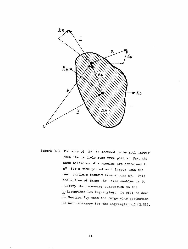
ID
R 1 1V
F
Figure 3.3 The size of AV is assumed to be much largerthan the particle mean free path so that the
same particles of a species are contained in
AV for a time period much larger than the
mean particle transit time across AV. This
assumption of large aV size enables us to
justify the necessary correction to the
V-integrated Low Lagrangian. It will be seen
in Section 3.5 that the large size assumptionis not necessary for the Lagrangian of (3.22).
44
where R is the random particle velocity with respect to v Since
v = dR/dt and F = mdv /dt, (3.18) simplifies to,D
dJ dxdv f m . x = AV Tr P + d fF (3.19)
AV AV
The left-hand side of (3.19) involves d(AV)/dt. In the case when this
is zero, e.g., in a stationary plasma, combination of (3.16) and (3.13)
then gives the expected expression,
U =Tr P . (3.20)R
This agrees with a result obtained by Gartenhaus (1961), who showed that
the collisional interaction potential of a stationary gas is proportional
to the particle thermal energy.
Combination of (3.16) and (3.20) gives a guess for £", at least
for the case when sufficiently frequent collisions can be assumed,
£" = V-U , U= Tr P + V.Q . (3.21)
Substitution of (3.21) in (3.12) then gives the total Lagrangian as
L = dx 1
V
E 2 B 2m nv2 (3.22)0M
nvD 2 M -Tr P - Q - qn( 2 ( 2 21o (3.22)
where the subscript M will be dropped from here on.
First,. we should point out that the assumption of a stationary
plasma in obtaining (3.20) can be relaxed for the purpose of obtaining
45
L in (3.22), if we let V tend to infinity. This can be seen by making
AV - dx in (3.19), and integrating dx over V -- , making the left-
hand side automatically zero because no particle now crosses the boundary
of V. Second, the assumption of sufficiently frequent collisions requires
that the size of AV be much larger than the particle mean free path. In
the following, it will be seen that this requirement is overly restric-
tive since the macroscopic quantities in (3.22) are well-defined in a
cell whose size need only be much larger than the mean particle spacing.
Further discussion of this point will be included in Section 3.4.
3.2.3 Application of Hamilton's Principle
We shall now test the validity of (3.22) by application of Hamilton's
principle. Note that L contains the generalized variables x (0t),
A (x,t), and P (x,t).
Variation with respect to A and y: The variation of L with
respect to A and y is comparatively simple since x is now treated as
an integration variable. For variations 6A and 6., which vanish on
the boundary of V and at times tI and t2, the Euler-Lagrange equa-
tions corresponding to
t2
I = dt L (3.23)
ti
take the standard form (Schiff, 1968),
a 'EA- 'L o (3.24)
46

where the functional derivatives of L with respect to A and c, in
Eulerian coordinates, are defined by
S3 1 (325)
Using (3.7) in (3.22), and then applying (3.24), leads to the Euler-Lagrange
equations,
aE- VX B = qnv , e V E = qn . (3.26)10O 0 at D 0
These equations, together with (3.7), form the set of Maxwell equations.
Variation with respect to 2: For x variation, the Lagrangian is
simply,
LE = dx E
V
E m 2 1S nv 2 1 Tr P - .Q -- qn( - v A) (3.27)2 D 2
where the superscript E signifies Eulerian coordinates, and the integral
of the electromagnetic field energy in (3.22) has been dropped because it
has no effect on the resulting Euler-Lagrange equation (Hill, 1991;
Galloway and Kim, 1971). The quantities vD, n, Tr P, and V . Q
are to be considered as implicit functions of x via subsidiary con-
straints. [Otherwise, the resulting Euler-Lagrange equation will be
a zero identity (Hill, 1951). ] These constraints are the first and
third moment equations derived from the Boltzmann equation (Braginskii,
1965),
47
af M dv-- + v f + -. f = C (3.28)t M dt vM
where C represents the contribution of elastic collisions. These are
the continuity and heat flow equations (Braginskii, 1965),
dn-- + nV .v = 0dt -
t (Tr P) + Tr P V.vD P:Vv+ . q = dv (v22v - D)C . (3.29)
The dyad notation will be used for dot products of adjacent vectors and
tensors. The continuity equation is equivalent to the mass conservation
law, the first expression of (3.4), used by Newcomb (1962), but the heat
flow equation is not in the form of a conservation law such as the second
expression of (3.4).
Virtual displacement method: A modified version of the virtual dis-
placement method used by Serrin (1959) and Lundgren (1963) will now be
employed to derive the variations of L from (3.29). This method consists
of introducing an arbitrary parameter, 6, into n (x,t;e), etc. The
corresponding nonlocal and local variations are then defined as, respectively,
'( ) (,t fixed, e = 0)
6( ) = (x,t fixed, e = 0) (3.30)
For our problem, it is more convenient to use t in this role, without
introducing e.
48
The nonlocal and local variations are defined in figure 3.4, from
which we can write
8'n(x,t) = n'(x',t) - n(x,t)
8n(x,t) = n'(x,t) - n(x,t) , (3.31)
with n denoting the density after the virtual displacement of
(v, t) = x-x (3.32)
Variation in vD: A schematic definition of 8'v and 8v is
shown in figure 3.5, from which we obtain immediately
, ,dx' dx d
D t -D(x 25) t ) dt dt dt
, d6-o= 6 o- o= dt - V , (3.33)
where (3.32) has been used to obtain the first expression, and Taylor
series expansion of vD'(x ,t) at x has been used for the second
expression.
Variation in n: We shall now use the first expression of (3.29)
to obtain the virtual displacement in n. First, we perform a real
displacement, Ax(xt), of a plasma cell in a short time period, At,
with the particles of the species in the cell conserved. This operation
is illustrated in figure 3.6, which shows both Ax and . Applying
the first expression of (3.29) along the path, Ax, we obtain,
49

(x',t)-
-n (xt)
n'(x,t) n (x,t)
(x,t)
Figure 3.4 The definition of nonlocal and local varia-
tions in n due to the virtual displacement
(xt). The nonlocal variation, 86n, is
defined by comparing n' with n for the
same cell, while the local variation, 8n, is
for the same coordinate x, before and after
the virtual displacement. The trajectories
of the same cell before and after virtual
displacement are denoted by - and --- ,
respectively.
50

S(x t)t)
Figure 3.5 The definition of nonlocal and local variations
in zD due to the virtual displacement (xt).
The nonlocal variation, 6 D, is obtained by
comparing v D with vD for the same cell, while
the local variation, 6v , is for the same coordi--
nate x. The trajectories of the same cell
before and after virtual displacement are denoted
by - and --- , respectively. The virtually
displaced trajectory that passes through (x,t)
is denoted by- - -
51

n'(x',t)
(x't)n'(x +Ax,t +At)
n (, txt)
Figure 3.6 The approach of a real displacement, Ax, performed
in a short time period, At, to the virtual dis-
placement, , as At diminishes to zero. Since
(3.29) describes the changes in n and Tr P/2
along the path Ax, the virtual displacements in
n and Tr P/2 are then described by (3.29) as a
special case At - 0 and Ax -.
52

-+ n Z~ =o An = (x+ Ax,t) - n(x,t) (3.34)At At
Since Ax and At are arbitrary, we can let Ax ( when At * 0.
Hence by definition, An, the change of n in the real displacement,
approaches the nonlocal variation 8'n. By cancelling At in (3.34)
before approaching the limit At = 0, we obtain
An - 6 'n -n V . (3.35)
The local variation in n is obtained by subtracting .Vn from 6'n,
giving
6n = -V •((n) (3.36)
Variation in (Tr P/2 + V. Q): The foregoing procedure can be applied
to any equation linear in d/dt and v such as the second expression
in (3.29). Caution must be exercised however, for those terms which do
not contain vD explicitly. From (3.29), we have along the displacement
Ax
1 1A(Tr P) + - Tr P V (x) + P :V(x) + (V g)At
- fv2C dv) At - m v (Ax)C dv (3.37)
When At - 0, the term (mfv2C dv/2) At will vanish if the macroscopic
displacement Ax does not significantly alter the microscopic random
processes within the cell. The term (V. q) At does not vanish: the
identity
53

v. ( = (V.Q)+ DV 3.38)
implies the relation,
(v.q)At = A(v.Q) + V(x): VQ (3.39)
Substitution of (3.39) into (3.37) before taking the limit At = 0, and
A = ', gives the following nonlocal variations:
6 Tr P + V. - Tr P V . - P: V : - V:V - Mv C dv (3.40)
The local variation corresponding to (3.40) is obtained by subtracting
* V (Tr P/2 + V .Q),
6(2 Tr + V.Q)= -V. Trp+ .i) v C dv . (3.41)
The Euler-Lagrange equation with respect to x: We are now in aposition to derive the Euler-Lagrange equation from LE by variation with
respect to x. The starting point is the integral of LE from time
t1 to t2-
I dt L(3.42)
t I
Because the integration variables are x and the time t (for fixed x),
local variations are to be used. The vector (x,t) is assumed to vanish
on the boundary of V, and at times tl and t2. Using (3.27), the
54

variation of (3.42) becomes,
fE = dt 6LE
t1
8LE = dx n[ vD2 c .A + n 6v D (myD+ qA) - 6 Tr P+ V.(3.43)
V
Substituting (3.33), (3.36), and (3.41) for 86Z, 6n, and 6(Tr P/2 + V. Q),
in (3.43), integrating by parts those terms involving ( L/ t) and V(,
dropping any surface integral that involves on the boundary of V,
and dropping any initial (tl) and final (t2 ) terms that involve _, we
obtain from (3.43) by straightforward manipulation the following result,
8L dx -mn(t + -74*P- ) n( p +
+qn( VA - D VA)- (mD +qA) + . (nv + m C dv (3.44)
Use of the dyadic relation,
vD X ( VXA) = VA - .DVA ,A (3.45)
and substitution of (3.7) and the first expression of (3.29) in (3.44),
finally gives the Euler-Lagrange equation as
dvmn dt + V.P = qn(E+ v XB) + mv Cdv , (3.46)
which we recognize as the macroscopic force law, with general pressure
tensor and elastic particle collisions (Braginskii, 1965).
In the above derivation, Q is not restricted any further than by
its definition in (3.16). The form V Q in the integrand of L is
not sufficient to make Q disappear from the final form of 8LE , since
Q is in general nonzero on the boundary of V. In arriving at (3.44),
however, it can be shown that Q appears in the integrand of 6LE only
in the form, V . ( .VQ), and hence drops out since vanishes on
the boundary of V.
3.3 Hamiltonian Density
When the independent (integration) variables of a Lagrangian, L,
are distinctly different from the generalized variables, and L is qua-
dratic in the time derivatives of the generalized variables, the
Hamiltonian, H, can be obtained by straightforward application of the
well-known Legendre transformation (Goldstein, 1950). The canonical
Hamilton system of equations is then obtained by varying each of the
generalized variables, and their conjugate momenta, separately.
For L of (3.22), however, the dual role of the variables calls for
additional care in formulating the correct Legendre transformation. If
the momentum conjugate to x is defined as
MLE v n(mvD + qA) (3.47)ZE Bv D=
by the use of (3.25) in the Eulerian coordinates, TE will be dependent
on x, because x is the integration variable. This violates the re-
quirement of the Legendre transformation that 6JE and ~ (= ) are to be
independent of each other. A way to avoid this difficulty is to trans-
form the integration variable from x to 2 S for that part of L
describing the particles, so that the integration is effectively performed
56

at t = 0. The dual roles played by A and C require that their
dependence on xSo be only through their explicit dependence on x (xSOt).
The momenta conjugate to the electromagnetic potentials must be defined
only in the Eulerian coordinates (x,t) (see Section 3.3.2).
The validity of the foregoing modifications to the Legendre trans-
formation will be established in Section 3.3.3, where the Hamilton equa-
tions will be shown to agree with the Euler-Lagrange equations obtained
in Section 3.2.3. After making similar changes in the definition
of the Poisson brackets, the energy equation is obtained correctly,
proving that the canonical formulation is self-consistent.
For completeness, a Hamiltonian corresponding to the Low Lagrangian
will be obtained in Section 3.3.6. The resulting total microscopic and
macroscopic energy conservation equations will be compared to help clarify
the meaning of the macroscopic potential, L.
3.3.1 Lagrangian Coordinates
In deriving their variational principles, Katz (1961) and Newcomb
(1962) used the transformations between x and extensively. These
transformation relations include, for x (~Ot), the Jacobian, J, the
transformation matrix, x.j, and its inverse matrix, Kij,
S1 xOj
J ij - x0j K (3.48)
whence it is easily shown that
J(JKji)- JK.. Kki x ij jk = dx =Jdx , (349)ij 0ki

where 8ij is the Kronecker delta with respect to the Cartesian
coordinate indices i and j, and the summation convention has been
implied. The initial value of n(x,t) is n 0 (0). By conservation
of particles along the cell trajectory, we have
ndx = n 0 dxO , nO = Jn (3.50)
Under these transformations, the Lagrangian, L, of (3.22) becomes
L dx I + eE B2
A- --U s Y- 2 2 ,OV0 V
s n - qn 0 (P-- A) - J Tr P +V . (3.51)
The time derivative, x (= dx/dt), used above is taken with fixed ZO.
The x-dependence of A and CP in the integrand should be retained,
in keeping with the dual roles of these variables.
The Euler-Lagrange equations with respect to A and T need not
be explicitly rederived in the Lagrangian coordinates (,0,t). They
should agree with those in the Eulerian coordinates since Hamilton's
principle is invariant under transformation of integration variables
(Courant and Hilbert, 19r3). The variation of L with respect to x,
however, should be re-examined, since x is no longer the integration
variable. To do so, only the part Ls, corresponding to a particle
species,
Ls dx1 s (3.52)
V0
58 U'

has to be considered. The standard form of the Euler-Lagrange equation
for x is then
d ( Ls
In Lagrangian coordinates, the functional derivatives of Ls with
respect to x and x have the forms
s s s s s a l
-- i =i xoj.axj X uj - ' -1 1 j 3i. 1 1 j ij
which may be compared to those for OL/OA, etc. in Eulerian coordinates
in (3.25).
The only part-in 1- whose partial derivatives with respect to x.s 1
and x. are unknown at this point is Tr P/2 + V .Q. To obtain them,
we use the heat flow equation, but in a different fashion from that of
Section 3.2.3. In Lagrangian coordinates, (3.29) becomes
Sd (Tr P)+ 1 Tr P V x+P:V ;+ V q = (2 - 2v . x)C dv (3. 5)
where the gradient, V, is to be read as Kji /ax 0j Replacing q
by the dyad identity (3.39) converts (3.55) to the form
Tr P + V .Q - (Tr )K Xij - P Kkj ik
bx kj ik ji i P ~-x .; xim x c dv+I v C dv
S --- ij Tr P+V Tr P+V .Q + -Tr P+V. , (3.56)
59
where the third formal expression is obtained by treating Tr P/2+ V. Q
as a uniquely determined function of x .(t), xi(t), and t. Thus,
by equating the coefficients of x.i and x., we obtain
+Yx .+ V - Tr P K - P K K--
xji ik jk x. jk
ax- TrP + V -m v Cv Cdv , TrP+V7.Q2 v2Cdv . (3.57)
These relations enable us to find expressions for BL /ax. by derivings 1
J s/ x and s /ax.i from (3.51). After some algebra, we obtain
A - - + Jf m v. C dv
Ka +Vkaj- jk axOj ik + ji ax V.Q Kjk axOj I ]
BL nO(m + q (3.58)
By replacing Kji /8x 0oj by / xi, we find that the two terms involving
Q in the first expression in (3.58) cancel each other. It is now
straightforward to use (3.49), (3.50), and (3.58) in (3.53) to show that
the resulting Euler-Lagrange equation is identical to (3.46), except
for a-multiplicative factor, J.
6o

3.3.2 Modified Legendre Transformation
Since x is no longer formally used as an integration variable in
(3.52), the momentum variable conjugate to x for each particle species
can be properly defined as (Schiff, 1968)
L
S- = no(mx + qA) , (3.59)
where the second expression of (3.58) has been used.
The momentum variable, 9, conjugate to A, must be defined
differently. It is reasonable to let 0 have exactly the same dual
role property as A has in L. The way to assure this is to make
(Zt), rather than ( O,t), the independent variable in the definition
of C.- Thus, we have
= ,(3.60)
which, by using (3.22), may be put in the familiar form (Schiff, 1968),
= o CPV + o = . (3.61)
A momentum variable conjugate to CP does not exist, because L does
not involve bcp/bt.
Since the conjugate momenta of (3.99) and (3.61) are defined in
Lagrangian and Eulerian coordinates, respectively, the Hamiltonian must
be defined by adding contributions separately from the plasma variables
(x,1) , and the electromagnetic field variables (A,G2p). It is given
by the following modified form of Legendre transformation
61
H = dO • x + dx - L , (3.62)
VO V
which is assembled in a similar form to the Low Lagrangian, LL in
(3.6), and the macroscopic Lagrangian, L in (3.51). Substitution of
L from (3.51), and elimination of x and A/ t by use of (3.59)
and (3.61), reduce H to the form,
H=[ d[ + + _xI + 1V O s d 80 2 0Vo V
s I2- qn 12 + qn 0 CP + J Tr P+ V ) (3.63)
Alternatively, H can be transformed to Eulerian coordinates by use of
the last expression of (3.49) and the first expression of (3.50),
H = dx ]
V
22+ I VxA12= - qnA 2 Tr P+ V . Q+ qn + - . . (364)
By use of (3.59) and (3.61), we have from (3.64)
VD + Tr P + V . Q + qnP) + e E + e . Vp , (3.65)(T,. 24 .0
which is the familiar form of energy density for a plasma, plus the term
V * Q. The latter represents all of the energy density lost through
heat conduction prior to time t, by a cell of a particle species, as
it moves along its trajectory.
62

It is of interest to compare H with that given by Schiff for a
quantum mechanical system of charged particles in an electromagnetic
field [Schiff, 1968, equation (57.4)]
HQM = dx ,QM
y 12 jVx A 2
= I(-iV - qA) 2 + qJ + + 2 a VCP+M M 2e0+ 2 ' (3.66)
now written in MKS units. In (3.66), Y and V. are the Schrodinger
wave function and potential, respectively, and -iV is the particle
momentum operator. With the understanding that Ii12 is equivalent to
particle number density, a term-by-term correspondence is observed
between (3.66) and (3.64), with the potential energy density V Jlj 2
corresponding to Tr P/2 + V .Q, in agreement with the interpretation of
the negative sign that the latter has in the macroscopic Lagrangian.
3.3.3 Hamilton Equations
The approach of Section 3.3.2 has been plausible. To establish
that the formulation is self-consistent, we should verify that the
Hamilton equations derived from H agree with the Euler-Lagrange equa-
tions derived from L.
Using (3.59) and (3.60), the Euler-Lagrange equations, (3.53) and
(3.24), become
EL EL i aL- ' , A. t O . (3.67)
The variation of L of (3.51),
63

6L= LL d( d[ 8A+ 8(6A) L1 (3.68)+ "A + d((a/t 8 , c3.68)Vo V
can be put in the form
6L= d ['( .x)+ .*-x.*8' + dx[6 * +.' -6A * ,6
0 (3.69)
where (3.59), (3.60), and (3.67) have been used, and 6 (6') is the
local (nonlocal) variation defined in Section 3.2.3. The variation of
(3.62) consequently becomes
8H = - d * d"xiA 6) . (3.70)t 6U0(3-70)
v0 V
Since the variables in H to be separately varied are x, T, A, , and
cp, it is convenient to write 8H as
6H= d *+ J gdx * 6A+ * acpi , (3.71)
V0 V
where the functional derivatives of H are analogous to those of L
given in (3.54) and (3.25).
Comparison of (3.70) and (3.71) shows that the correct forms of the
Hamilton equation for macroscopic plasmas described in terms of variables
with dual role, are
aABH ~ H
- 1 ' - '(3.72)
which are identical to (3.59) and (3.61), and
64

- x t - .= o (3.73)
The last two expressions of (3.73) lead to (3.26) by straightforward
differentiations of (3.64) before using (3.61). The right-hand side of
the first expression of (3.73) can be written as -# /.x. +s 1
(a/xoj )(s /x ij). Its first term can be derived from (3.63) as
Oj s A j
xs ( --qn 0 A ) + qn0 Jmv C dv (3.74)1 1 1
where the second expression of (3.57) has been used. Its second term
can be shown to be
Ss Ik- ik= JK JK JK-ap a - -J ap(3 aka x xa x 'ak)x (375)
;xOj ij x0j k J xj _gi
where the first and third expressions of (3.49), and the first expression
of (3.57) have been used to obtain the first result, and the relation,
a/ax. = K. j /Bxoj, has been used to obtain the second result. It is1 1Ji
then straightforward to show that the first expression of (3.73) is equiva-
lent to (3.46) by the use of (3.75), (3.74), (3.59), (3.45), and the
relation, = v
3.3.4 Poisson Brackets
Poisson brackets are convenient in writing down the time derivative
of a physical quantity in a system that is formulated in terms of a
Hamiltonian. They must also be modified on account of the dual role of
the variables. Consider in general a physical quantity G, which is a
functional of x , A, O, , and their first derivatives. Without
loss of generality, we may write
G dx = dO + fdx EM , (3.76)
V VO V
where gEM is a function of A, Cp, and their first derivatives, only,
and contains terms that must involve x, I, their first derivatives,
and Tr P/2 + V *Q. The time derivative of G can be obtained by
accounting for the dual roles played by the variables, x, A,
and CP. in G. This requires that
dG cd dg s= 1dx dx , (3-77)
Vo V
where, in the right-hand side, the first time derivative is defined with
A, a, and CP treated as given functions of x, and the second time
derivative is defined with x and treated as constants. Use of the
Hamilton equations, (3.72) and (3.73), transforms (3.77) to
sdt- t d .s + -f do * (3. 78)
S S
where the plasma and electromagnetic field Poissoh brackets, and the
functional fluxes, Is and , are defined by
66
9 G .H G BH G P
V
-j -_ X- B(aj /ax
aA. 2
j a(A s/ax 7 at a(a_ _ t (i3A.I 3 A-x -+ +(/axj ) -t- '(BP/x) -t (3.79)
In the integrals of (3.78), s0 and S are the bounding surfaces of
V0 and V, and d0 and do are the elementary surface areas, with
vectors taken along the outward normals. The partial time derivative,
8G/6t, takes care of any explicit time-dependence that G may have in
addition to its implicit time-dependence through x, T A, Z and (P.
3.3.5 Energy Conservation Equation
Equation (3.78) can be used to formally separate the time deriva-
tive of any physical quantity into the bulk and the surface contributions,
and the plasma and electromagnetic field terms. As a demonstration that
the foregoing formulations are self-consistent, the total energy con-
servation equation is derived by substituting H for G in (3.78).
We obtain
dH + M = d (3.80)
So S
where the plasma and electromagnetic energy flux densities, ys and
ZE, respectively, are given by
67
sj i[jk( ik + K k
JEM X B - eE - (3.81)
A more familiar form may be obtained from (3.80) by use of the third
expression of (3.48) and (3.49), and the second expression of (3.50).
After some manipulation, we have
dddt - (v Q d) + dx(V. - 0
aAS= (P. +q) 1 X B E (3.82)
By use of the identity,
- (dx) dx(VO ) , (3.83)
and the differentiation scheme of (3.77), we can further transform (3.82)
to the following form in Eulerian coordinates,
a (-ZV.Q) + V. != 0
Et- v D + Tr P) + P D+ S + - EXB (- E) (3.84)
Since 4 - E V. Q is the energy density in the plasma at time t, (3.81),
to which (3.84) is equivalent, is the correct expression of energy con-
servation in the mixture of Eulerian and Lagrangian coordinate systems.
68
It is also possible to derive (3.84) by evaluating a/Bt from (3.65),
and then using (3.20), (3.46), and Maxwell's equations.
The derivation of (3.84) completes our development of a self-
consistent Hamiltonian description of a plasma in the macroscopic
approximation; the difficulties associated with the dual role of the
variables in the description of the field-particle system, originally
pointed out by Sturrock (1958a), have been resolved. Since the Low
Lagrangian also assumes 'dual role, the microscopic Hamiltonian descrip-
tion of a Vlasov plasma can also be established in a similar fashion, as
will be shown briefly in the next section.
3.3.6 Microscopic Hamiltonian Density
By the use of the Low Lagrangianin (3.6) and (3.10), the conjugate
momenta can be defined in forms analogous to (3.59) and (3.60) as
LL - m +qAS(oo, t) , mx qA(xt) ,
aL aL F LV: Ba( x,t) A/t) = -A/at/ - [ o ,V4 A t (3.85)
where the second expression for _ follows because * does not involve
a/bx0 and a/VO terms.
The corresponding Hamiltonian is defined analogously to H as in
(3.63),
HL = dv f( , x + dxa - LL (3.86)
V0 V
69

After some manipulation, this takes the form
HL E dx~ dvo f (O,)h + dIx 2 0 .*
V0 V
1 2h 2 -qm + q.
The Eulerian form of HL can be obtained from (3.87) by use of (3.9),
HL = dx L ,
V
L f ,vt v2 + q + 2 + + eEvP . (3.88)L= 2 2 2p 0
With the definitions of (3.85), the Euler-Lagrange equations of LL
are
L L L LAx - A at ' cp (3.89)
These can be shown to represent the microscopic particle force law and
Maxwell's equations. Taking the variation of HL, and using (3.89),
the Hamilton equations are easily obtained as
aHL aA HL OHL 2 HL HL
tx t - A a cp =
(3.90)
Since HL does not involve the derivatives of x and with
respect to x: and v0' it suffices to consider a physical quantity,
70

G, for plasma with the same simplification. We may write
G = dx (x, ; , A,9Cp)
V
x d vZfd o f(o,O) s(x,_) + (dx E(A,,C) . (3.91)
VO V
The expression for dG/dt analogous to that of (3.78) is then obtained
as
dtG - GH+LG) - d *FE (3.92)LI P I L EM V ;.- '.V
where the microscopic Poisson brackets, and 'f j, are defined by
GH f(Lx=) dG* - *
VO
($G BH _G WHL MG SmG, H dx +
V
- + + (393)andE j at a(apAax.) a a(mpax. at a(acax) (3-93)
The energy conservation equation in the microscopic plasma model is ob-
tained by replacing G by HL in (3.92). We obtain
dH LAL 1
+ d IL = O L - 0 t X B - eE "7 (3.94 )
dt ko at ( 3.94V
By use of (3.88), the following is obtained from (3.94)
71
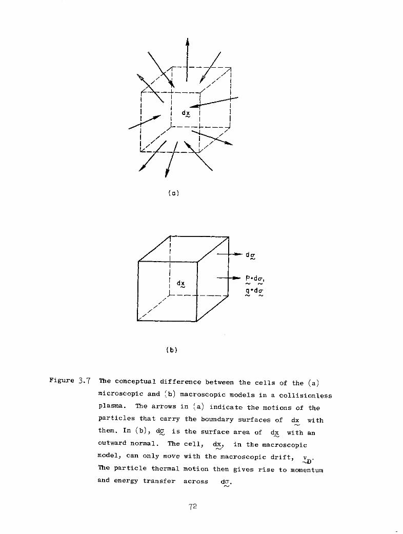
/7
-< I
dxI
(b)
,H / -oo
(b)
The particle thermal motion then gives rise to momentum
and energy transfer across do.
72

(dx L) + dx(V . = 0 . (3.9dt XIL
A comparison of the energy conservation equations in the microscopic
and macroscopic models, (3.99) and (3.82), respectively, can be found
in Section 3.4.3.
3.3.7 Entropy for Plasmas
In this section the Lagrangian and Hamiltonian formulations have
been developedso far,for the purpose of obtaining self-consistency and
consistency with the well-known equations describing plasmas in the
macroscopic model, e.g. the force law, Maxwell's equations, and the
energy conservation equation. Now, the dual role approach has resulted
in a canonical formulation of plasma dynamics in which the plasma and
electromagnetic field variables are all treated as canonical variables.
It is proposed that these canonical variables may also be effectively
used to express other plasma quantities of interest, such as the appro-
priate plasma entropy.
The question of whether the Gibbs or the Boltzmann H-function is
the correct definition for a many-particle system with arbitrary inter-
particle forces, has been discussed by Jaynes (1965).. He concluded
that an appropriate definition of entropy must include all of the degrees
of freedom that we intend to use for the physical system. In this
section, the number of degrees of freedom equals the number of generalized
field-like variables. Thus an appropriate expression for entropy in the
macroscopic plasma model can be obtained only in terms of all of the
generalized variables and momenta. Since the Boltzmann H-function, in
73
its hydrodynamic form (Braginskii, 1965),
S = n , S = n (Tr P) (3.96)
is defined without including the degrees of freedom associated with the
electromagnetic field variables, it clearly does not represent the total
entropy of a plasma in the macroscopic model.
Consequently, the Boltzmann H-theorem is likely to be violated in
plasmas whenever the process involves an appreciable change in the electro-
magnetic field energy. This conclusion agrees with recent results of
Jaynes (1971), who has shown that the necessary condition for violating
the Boltzmann H-theorem is that the initial kinetic energy associated
with particle velocities, both drift and random, be greater than the
equilibrium kinetic energy. The difference is then converted into
potential energy, associated with particle interaction forces, both
collective and random, during the evolution towards equilibrium.
An important question which we have not had time to pursue is the
nature of an appropriate expression for plasma entropy based on the
canonical models established in this section.
3.4 Discussion of the Macroscopic Potential, V
In this section, we have been mainly concerned with a rigorous
verification of the Lagrangian and Hamiltonian formulations for a plasma
in the macroscopic model. However, in order to obtain the correct
macroscopic Lagrangian, a heuristic argument that assumes sufficiently
frequent particle collisions was used in Section 3.2.2.
74

This assumption was in turn found to be overly restrictive because
the macroscopic Lagrangian and Hamiltonian, verified in Sections 3.2.3
and 3.3.3, respectively, are equally applicable to a collisionless
macroscopic model when the moments of the Vlasov equation are appro-
priate. Therefore, it is of great interest to find a reasonable
explanation for the necessity of introducing U of (3.21) also for
the collisionless macroscopic plasma model. We shall proceed by con-
sidering the relation of V to viscosity and heat conduction first.
3.4.1 Relation of V to Viscosity and Heat Conduction
According to (3.21), V represents twice the thermal energy density
of a particle species plus the energy density lost due to heat conduc-
tion by a macroscopic plasma cell, as it moves along its trajectory.
The relation of V to viscosity and heat conduction can be further
demonstrated by considering the particles of a species in a macroscopic
cell, dx, that has a size much larger than the mean particle spacing
and follows some trajectory in the plasma. By the use of (3.83), (3.29),
and (3.38), the total time derivative of V within dx is given by
S(dx U) = dx -2P:Vv +m(v 2v ,v)C d + V- 2q , (3.97)dt Iat (
The first term in the right-hand side brackets represents twice the time
rate of heat generation in dx due to viscosity and mechanical compression
(Braginskii, 1965). The second term is twice the time rate of heat
generation in a particle species resulting from collisions with particles
of other species. The third term contains twice the rate of energy
gain due to heat conduction.
75
If (3.97) is integrated over V, before summing over all species of
particles, the collisional term will drop out because of conservation of
energy and momentum in elastic collisions. Equation (3.97) then becomes
d- . Q+ -2q (3.98)
V V
The phenomena of viscosity and heat conduction, which are usually regarded
as dissipative, are being compensated for. The total energy of the plasma
in the macroscopic model, as denoted by H in (3.63)-(3.65), is con-
served through the inclusion of -V in X' of (3.12).
3.4.2 Loss of Particle Discreteness in Applying Macroscopic Approximation
Equations (3.97) and (3.98) are applicable also in the case when
collisions are negligible, e.g. in the macroscopic approximation
of a Vlasov plasma with the size of dx much larger than the mean
particle spacing. In this case, the argument of Section 3.2.2 that leads
to the expression for U is no longer appropriate because the assumption
of frequent particle collisions within dx is no longer valid.
The following question consequently arises: why is it still necessary
to include V in 1L, in the macroscopic approximation of a Vlasov
plasma, to obtain the correct macroscopic Lagrangian, L, of (3.22),
now that UR in (3.15) can no longer be considered as the energy
associated with particle collisional interactions? This question suggests
the following argument; that it is actually the loss of particle dis-
creteness in applying the macroscopic approximation of (3.12) which must
be compensated by the correction expressed by (3.15).
76
In the collisionless microscopic model, the trajectory of each
particle is, in theory, to be solved. When the Low Lagrangian is
written, the cell dx is used for the purpose of summing the contribu-
tions of particles within dx. Owing to the assumed particle continuity
in phase space, the bounding surface of dx in this model is considered
completely flexible; if dx is cubic at time t, we can, in theory,
always deform the shape of dx to include the same particles at some
later time. This definition of dx is illustrated in figure 3.7(a),
which implies that, in the microscopic model, as long as the particle
trajectories are solved, there is no momentum and energy transfer
across the flexible boundaries of dx. In the macroscopic model, however,
particles of the same species are indistinguishable. Only the spatial
coordinates of the macroscopic cell, dx, can be used to identify the
plasma, as shown in figure 3.7(b). Although moving with the drift velo-
city, D' the macroscopically smooth boundaries of dx are penetrated
by particles due to thermal motion. This then gives rise to the well-
defined outward macroscopic momentum and energy transfers V * P dx and
V *q dx, rexpectively, from dx. Furthermore, since elastic collisions
conserve momentum and energy, they do not affect these macroscopic trans-
port phenomena. In terms of these momentum and energy transfers, the
dynamics of the cell, dx, and that of a cell, BV, introduced in
Section 3.2.2, become identical. The macroscopic potential energy of
(3.15) must correspondingly be introduced for a collisionless macroscopic
plasma.
77
3.4.3 Definitions of Plasma Cell Boundary
That the microscopic and macroscopic models define the boundary of
a spatial volume differently can also be seen by comparing the micro-
scopic and macroscopic energy conservation equations, (3.95) and (3.82),
respectively. We see that the difference between the microscopic and
macroscopic energy flux densities, !L in (3.94) and F in (3.82),
respectively, is the flux density, E (PZ -+q), associated with
particle thermal motion. Mathematically, this flux density is absent
in _L, because the microscopic Hamiltonian, HL in (3.87), does not
contain any derivatives of x and _ with respect to x and v
Physically, this difference between (3.95) and (3.82) is attributable
to a difference in defining the microscopic and macroscopic plasma cell
boundaries.
Consider the time derivatives of HL in (3.88) using two different
definitions of the volume, V. First, define V as a stationary volume.
We have,
/ 2HL + xxd-2+ q + + e * , (3.99)
St at at 0 2 'V 2
which can be reduced to the macroscopic energy conservation equation,
(3.82), by use of the Vlasov equation, Maxwell's equations, and integra-
tion over velocity space (Van Kampen and Felderhof, 1967). Second,
define the boundary of V as moving with the enclosed particles, so that
the Liouville theorem can be applied. We then have
d xdv f(x,vt) = ddx dvo f(x0,0) = constant , (3.100)
V V0
78
because of (3.8). The total time derivative now becomes,
dHL dv d dx--+ B 2 +d L- dx dv f my *+d( fdx(--+ + E + Vp) (3.101)
V V
which can easily be reduced to the microscopic energy conservation equa-
tion in (3.95) by use of the particle force law, Maxwell's equations,
and integration over velocity space.
Since these energy conservation equations, (3.95) and (3.82), are
also derivable from their corresponding Hamiltonians, (3.87) and (3.63),
which are in turn derived from the corresponding Lagrangians, (3.6) and
(3.51), it is seen that the difference between the Low Lagrangian, LL,
and the macroscopic Lagrangian, L, is to reflect the difference in
defining the microscopic and macroscopic volumes (or cells) and their
boundaries.
3.4.4 Relations Among the Variational Principles of Various Models
The arguments of Sections 3.2.2 and 3.4.1 - 3.4.3 are helpful for
the purpose of understanding the macroscopic Lagrangian, L, and potential
energy density, U. The relation between these viewpoints can be under-
stood from figure 3.8, which compares the plasma variational principles
of the collisional and collisionless microscopic models defined in
Section 3.2.1, and the macroscopic model. Procedure 1A involves dropping
the random terms defined in (3.11) to relate LT to LL, while
Procedure IB involves only smoothing within the macroscopic cell, dx,
as described in (3.12), to obtain LT from LT, by keeping the quadratic
random terms. Procedure 2 reflects the difference in definitions of
the plasma volume, V, or cell, dx, in the microscopic and macroscopic
79

Euler-LagrangeApproximate
EquationsModels: Equations Liouville'subsidiary
(constraints) Laws
Collisional EL.T. H.P. Particle Force Law One-Particle
Microscopic T T Particle continuit Liouville'sin Phase Space Law
1A 1A 1A 1 1B
CollisionlessEc .. P. Particle Force LawCollsionessECE H L.T. L LP article.i Vasov BoltzmannMicroscopic L in Phase Space Equations Equation
00) (2 dv0
Sdv fjdvMacroscopic Force
Macroscopic E.C.E. H T H L LawContinuity and HeatBalance Equations
Figure 3.8 Relations among the variational principles of various plasma models. Here
LT and HT represent the total Lagrangian and Hamiltonian, respectively,
in the collisional microscopic model; LL and H L represent the (Low)
Lagrangian and Hamiltonian, respectively, in the collisionless microscopic
model; H.P. represents Hamilton's principle; L.T. represents the Legendre
transformation, and E.C.E. represents the total energy conservation equation.

plasma models, as discussed in Section 3.4.3, with regard to the energy
conservation equations in the two plasma models. In the case of a
collisional plasma, Procedure 3 represents the heuristic approach of
Section 3.2.2 that led to the appropriate expression of U in (3.21).
For a collisionless plasma, Procedure 4 represents the argument of
Section 3.4.2 that discusses the loss of particle discreteness when we go
from the microscopic model to the macroscopic model, and the dynamic
equivalence between the macroscopic cells of the collisionless and
collisional plasmas, so that the introduction of 1 is seen to be
necessary also for the collisionless macroscopic model.
All of these arguments should be considered less rigorous, for the
purpose of proving the validity of L of (3.22), than the rigorous
verification by application of Hamilton's principle in Section 3.2.3.
These different viewpoints do, however, converge to the conclusion that,
in general, the macroscopic potential energy density, 1, is a result
of the combined contributions of plasma fluctuations (which is equiva-
lent to elastic multiparticle collisions), elastic two-particle collisions,
the loss of particle discreteness, and a redefinition of the plasma
cell, d x, in the process of making the macroscopic approximation.
3.5 Discussion
The principal contributions of this section verification of an
appropriate Lagrangian density in Section 3.2.3 and Hamiltonian density
in Section 3.3.2 for the macroscopic plasma model, including a pressure
tensor, heat conduction, and elastic particle collisions. In Section 3.3.2,
it was shown to be necessary to introduce a macroscopic potential energy
density ) (= Tr P+ V .Q). In order to obtain the Hamiltonian density,
81

it was necessary to modify the conventional Legendre transformation to
conform to the dual role of the generalized variables. Low's Lagrangian
(Low, 1958) shares the same property; the modified Legendre transforma-
tion was used successfully to derive a corresponding Hamiltonian in
Section 3.3.6. The modified form of the Hamilton equations and Poisson
brackets presented in Sections 3.3.3 and 3.3.4 may have further interesting
implications in the canonical formulation of plasma dynamics.
The plasma model used in this section is, of course, a macroscopic
approximation to the microscopic model described by the Boltzmann
equation, or the Vlasov equation when collisions are negligible. The
Euler-Lagrange equations, (3.26) and (3.46), consequently have a one-
to-one correspondence with those of the Low Lagrangian. The continuity
of particles in phase space, (x,v), is used by Low to constrain the
variation with respect to the particle trajectory, x (:,ov ,t), while
here the first (particle continuity) and third (heat balance) moment
equations are used to constrain the variations with respect to the
plasma macroscopic cell trajectory, x(xo,t). That only two moment
equations are sufficient here does not imply that the mathematical system
is closed at the second order moment equation. What we have done is to
apply Hamilton's principle to a mathematically open system of equations:
the Maxwell equations, and the moment equations. The latter are not
truncated, since q appears in the heat flow equation, and can only be
obtained by use of higher order moment equations. In practice, trunca-
tion will be accomplished by making some arbitrary assumption about q,
typically q = 0.
Whenever the scale length of variation of the macroscopic quantities
becomes comparable with the mean particle spacing, the results presented
82
in this section for the macroscopic model becomes questionable. In addi-
tion, the assumption of elastic collisions neglects excitation, ioniza-
tion, and recombination phenomena, and electromagnetic radiation
associated with charged particle collisions (bremsstrahlung). Never-
theless, the variational principle developed here is appropriate to a
multicomponent plasma, including neutral components.
In later sections, we shall apply our results to a number of plasma
problems involving perturbation expansions. While these are straight-
forward for v and n (Newcomb, 1962), difficulty arises in connection
with the term Tr P/2 + V *Q in S. Inspection of the heat flow equa-
tion in (3.29), reveals that it is not self-consistent: even with an
explicit form given for C, we have to solve for all of the elements of
P as well as the components of q; these depend on higher order moment
equations. Even when truncation at a specified moment of the Boltzmann
equation is assumed, the heat flow equation is not generally equivalent
to some constant of motion for a particle species. For the case in which
q and C are neglected, approximate expressions for P in terms of
the perturbation in x are generally impossible to derive mathematically
(see Section 4.2.2). It is not surprising that only problems in which
collisions between different particle species are neglected, and adiabatic
processes are assumed to occur with either a scalar or axisymmetric
pressure, have been successfully studied in terms of perturbation expan-
sions. Such problems form the subject of Section 4.
83

4. THREE-WAVE INTERACTIONS: THEORY
4.1 Introduction
In this section, we shall show how the macroscopic Lagrangian ob-
tained in Section 3 can be applied to the description of nonlinear
wave-wave interactions in homogeneous plasmas. After developing a
perturbation expansion of the Lagrangian, the method of averaged
Lagrangians will be employed to derive general coupled mode equations.
In Section 5, these equations will be specialized to a number of cases
involving parametric amplification of ion-acoustic waves for which
experimental data are available.
The use of Lagrangians in describing nonlinear wave phenomena
was considered by Sturrock in 1961. He showed that in a conservative
distributed system the time-averaged Poincare invariants, which he
later extended to the case of field variables (Sturrock, 1962), are
equivalent to power-balance relations of the type well-known to electri-
cal engineers as "Manley-Rowe relations" (Penfield, 1960). These results
were extended by Whitham (1965) who averaged the Lagrangian in such a
way as to remove rapidly varying terms, but conserve the slow variations
in amplitude, frequency, and wave vector characteristic of a wave train
in a weakly nonlinear medium. Vedenov and Rudakov (1965) used this
approach to describe the interaction between ion-acoustic and Langmuir
waves in a plasma. Using Low's Lagrangian (Low, 1958) and its pertur-
bation approximation, several cases were examined by Suramlishvili,
who derived the wave coupling coefficients for interactions between Langmuir
and ion-acoustic waves (Suramlishvili, 1964), between one transverse
and two longitudinal waves (Suramlishvili, 1969), between Alfvn and
84
whistler waves (Suramlishvili, 1967), between Alfvn and ion-acoustic
waves (Suramlishvili, 1970), and among magnetoacoustic waves
(Suramlishvili, 1971). A variety of general results have been established
by Galloway (1972) and Dysthe (1974), using the averaged Lagrangian
method. In particular, the former demonstrated that the energy conservation
equation may be used to derive the Manley-Rowe relations, and the
coupled mode equations describing wave-wave interactions. He has also
shown that the wave energy and energy flux follow directly from the
energy and energy flux terms quadratic in the perturbations, while the
nonlinear wave coupling coefficient follows directly from the term in
the Lagrangian cubic in the perturbations. Similar general results were
employed by Boyd and Turner (1972b), who used Low's Lagrangian to examine
the generation of longitudinal plasma waves by two high frequency electro-
magnetic waves in a warm field-free plasma, and the interaction of
three electromagnetic waves in a cold magnetized plasma. This approach
will be followed in Section 4.3.
Generalizations of the averaged Lagrangian method to nonlinear plasma
phenomena other than wave-wave interactions have been made. Using a
hydromagnetic Lagrangian derived by Newcomb (1962), Dewar has shown that
the interactions between the wave and the slowly varying background
plasma may be derived by use of Hamilton's principle (Dewar, 1970).
Dougherty (1970) has obtained ray tracing and coupled mode equations, and
demonstrated the conservation of wave action in a relativistically
covariant formulation. Four-wave interactions, self-action effects, and
sideband decay phenomena have been treated in the paper by Dysthe (1974)
mentioned above. Derivations of the wave kinetic equation have been
85
supplied by Suramlishvili (1964; 1965) and Galloway (1972); the latter
has also provided a description of quasilinear wave-particle inter-
action. A Lagrangian theory for nonlinear wave-packets propagating in
a collisionless plasma has been developed by Dewar (1972) which describes
the nonlinear frequency shift, Landau damping, and modulational sideband
instabilities.
It will be clear from the foregoing remarks that the averaged
Lagrangian method has been utilized to discuss many of the significant
nonlinear phenomena occurring in plasmas. It has the merits of concise-
ness and efficiency in the analysis, and gives considerable insight
into the physical mechanisms involved.
4.2 Perturbation Approximations to L
Prior to its use in Section 4.3, we shall expand the Lagrangian,
(3.22), in terms of perturbations in the generalized variables, x, Cp
and A, up to the third order. Similar to the well-known approach for
the macroscopic Lagrangian (Newcomb, 1962), the perturbations in n,
ZD1 and Tr P/2 + V .Q will be considered as due only to those in the
generalized variables. Denoting the perturbed and unperturbed Lagrangians
by L' and L, respectively, we write
LI = L + L1 L2 + L+ ... , L i Idx 'Li (4.1)
V
where Li denotes the Lagrangian ith order in perturbations. The qua-
dratic Lagrangian, L2, will provide the first order equations that
determine the linear wave properties, and the cubic Lagrangian, L3' will
lead directly to the nonlinear coupling coefficients among the waves.
86
4.2.1 Definition of Perturbations
The perturbations in the generalized variables are defined as,
x + xt) CP, c P+ Y1 A'= A+ A (4.2)
where (x, P), A) and (A 41' A~) are the unperturbed and perturbation
variables, respectively. Figure 4.1 illustrates the definition of ~,
which is analogous to the particle displacement vector defined by Sturrock
(1958a) and Low (1958), and the macroscopic cell displacement vector
defined by Newcomb (1962). The quantities (cp, A) and (cp1 A ) are
considered as functions of the Eulerian coordinates (x,t). consistent
with their dual roles discussed in Sections 3.1 and 3.2.1.
The perturbed Lagrangian differs from-the unperturbed Lagrangian
(3.22) due to two factors: first, the presence of , 91' and A1 at
a given , and second, the use of the integration variable x rather
than x. Thus the perturbed Lagrangian may be written as
=L' dx' £,
V
•2' 2
'. Tn v2 1 Tr P" - 9*Q -qn" D'*A + O B20D 2 2 2pO
where the summation applies to the particle species. In (4.3), and what
follows, primed and unprimed quantities are functions of x' and x
respectively, unless otherwise noted.
Imposing the condition that the particles are conserved in the
process of applying perturbations, implies that,
87

Sn( ,t)
Figure 4.1 The definition of perturbation in the macroscopic
plasma cell position from x to x'. The perturba-
tion is performed in such a way that the number of
particles of a species in the cell is fixed. The
perturbed and unperturbed cell trajectories are
denoted as and ------ , respectively. The cell
velocities before and after perturbation are denoted
by v.(xt) and v(x',t), respectively. The velocity
of the cell that is at (,t) after perturbation is
denoted by v(:t).
88

ndx = n'dx (4.4)
while the Jacobian, J, of the transformation from x to x is
dx
dx
The integral in (4.3) can consequently be written in terms of an
x-integration as
L= dx 1
V
£=[nvD2_ J Tr P + V*Q') - qn( A-IA' + ( - . (4.6)
4.2.2 Expansions of v, n , and P
The terms that involve vD J, ', A', E', and B are easily expanded
by the use of (4.2), (4.4), and (4.5), and the Taylor series expansions
at x. However, expansion of the terms, Tr P /2 + V *Q , in (4.6)
introduces considerable difficulty. We shall confine ourselves to the
case of scalar pressure and adiabatic processes satisfying the equation
of state
p n ijP
for each particle species, with Y being the adiabatic index.
89
Expansion of zD: Taking the time derivative of the first expression
of (4.2), we obtain
vD= v + ; (4.8)
where % denotes dj[x(,o,t),t]/dt. Then the nonlocal expansion of
vD is seen to be,
vD =D+ v+ v2+ v3+ ... ,
vv = = O (4.9)-1 : , 42 -3
If we define the local expansion of v'(x,t) as
Z (x t) = + VL + L2 L3+ ... , (4.10)
it can be shown by Taylor series expansion of v'(x',t) at x that
i
v. = .i + . (" V)i v (4.11)j=l
As a result, we have
VL1 = - , vL2 = -" V + - -:VV,- + " V* . V . (4.12)
Expansion of n': Combination of (4.4) and (4.5) gives the particle
conservation law along as (Newcomb, 1962)
nJ = n (4.13)
90
With the Jacobian, J, expressed in -its exact expansion,
J I + V + IvV+11 \ I
(VJ - + V- V 17j Vj: + V (4.14)
the nonlocal expansion of n* becomes
n - n + nl + n2 + n3 +...
n = -nV n 2- + V:Vn31 -2
By use of a relation between ni and nLi analogous to (4.11), the local
expansion of n then takes the form
n (x t) = n + nL + nL2 + nL3 + ...
nL1= -V * (n) , nL 2 = - :( ~ ) .(4.1)
The results of (4.16) agree with Sturrock's generalization of the
Lagrange expansion in the form (Sturrock, 1960b)
nL. i! k " k "' n)(k,j = 1,2,3; i = 1,2, ... ) , (4.17)
while nLl and nL2 have been derived by Newcomb (1962).
91

Expansion of P': The nonlocal expansion of P' can be obtained by
substituting (4.1) and the second expression of (4.14) in the first
expression of (4.7),
P = P+ P1+ P2 + P3 +...
P = -yp(v . ) , P 1 P [ ( * V2'2 2
2P,- Y (V2 )3+ 7F)(v e + Q7
By use of a relation between P. and PLi analogous to (4.11), we obtain
from (4.18),
P(x,t) P+ P + PL L2 +
PL1 = -yPV -. VP
PL2 = [2 (v.) 2 + :V .
+ k [- + y(v • , + VP+ :VVP (4.19)
Because ZvL3, nL3 , and PL3 will not be needed to derive the second
order expansions of the perturbed force law (3.46) and Maxwell's equations
(3.26), these local expansions of vd, n', and P were not given
in (4.12), (4.16), and (4.19). The nonlocal expansions, v 3, n3 , and
P3, however, are included in (4.9), (4.1), and (4.18) because they will
be used in deriving L3.
92

4.2.3 Expansion of the Lagrangian
The expressions for the £. of (4.1) can be obtained by substitution
of (4.8), (4.14), (4.18), and the second expression of (4.7) in (4.6).
Thenfor the unperturbed Lagrangian density, we have
m 2 p e n0.AD E2 B2= nvD - qn( -A) + - - (4.20)
y-l
where the term P/(Y-I) is a result of generalization from P - 1
by replacing 5/3 by Y (Newcomb, 1962). For the perturbation Lagrangian
densities, we have after using integration by parts,
nD+ PV*.-qn(pl+ Vq(P- "A)+ qnvD 1(+ *VA) + E BlB1 ,
£2 = n 2 [(-1)(V)2 + VV:V - qn(~. + I VV
S 2 2
2 + 2 2
£3 -C [pl) (-v.) 3 + y! (.V)(V3:V0 ) +
+ qn * :VVA1 + 1~ :VVA) + .VA1 + 1 V A):V . (4.21)
The Euler-Lagrange equations of L, from I of (4.20), with respect to
x, A, and cp, are the unperturbed force law and Maxwell's equations,
93
mnvD + VP- qn(E + v X B) = 0
aEVX B- O B qnv = , EE- qn 0 . (4.22)
Use of these shows that L 1, from £1 of (4.21), is identically zero.
The Euler-Lagrange equations of L2, from £2 of (4.21), form the
system of linear equations in , Al, and cpl, describing wave propagation.
We shall not derive them at this point, but consider the Euler-Lagrange
equations resulting from variation of L2 + L3, describing nonlinear
wave-wave interactions.
Variation in P1: Taking the variation of L2 + L3 with respect
to (1 yields
e0V'E 1 + q (n) - VV(:(n = 0 (4.23)
Local expansion of the second expression of (3.26), and use of the last
expression of (4.22), gives
e0 V E1 - q(nL1 + nL2 )= 0 . (4.24)
By use of (4.16), it is easy to demonstrate that (4.23) and (4.24) are
identical.
Variation in AI: Taking the variation of L2 + L with respect
to A yields
o '7 - oa - q i- v(n ) - o(n )+ v:(n =0 . (4.25)
94
Local expansion of the first expression of (3.26), and use of the second
expression of (4.24), gives
OVX -1 q n + + nv + vL + nL2D = 0. (4.26)40 -1 0aLt nLl,D nI nL Ll 1,"
Use of (4.12) and (4.16) shows that (4.29) and (4.26) are identical.
Variation in $: Taking the variation of L2 + L3 with respect to
Syields
mn - (Y-1)VP V *(- *VP+ yP Y-1))(V- ) V(V*(+ V(V : V )+ V *V(V*.)
+ -1 VP[(Y-l)(V*)2 + : (Y-1)(V.)V.7P + VP
- qn 1 + .VE+ v X'B1 - B XV + B1 ~D -1 ~ +D
- qn VE+ + :VVE v :V)X - B1 +.VB X =0 . (4.27)
The local expansion of (3.46) at x, with V *P replaced by VP,
does not agree with (4.27). The discrepancy occurs because the former
is inconsistent with the nonlocal expansion of L' of (4.3). The
appropriate expansion of the force law must be constrained by the particle
conservation law, i.e. by comparing the first expression of (4.22) with
the force law
dv'J mn Z t+ V'P - qn (E'+ v X B = , (4.28)[ dt
95

which describes the same cell of particles in its perturbed motion.
The nonlocal expansion of (4.28) is
+ 1 L
mn ( + P - ( ) 2 (VJ:VJ)
+ + v + 1 ( 25 -1 (VE:V ) PL1+ VVP+ VPL 2 + S*VVL E
- qn ( 1+ + 1E'VEI+ e:VVE - qn XB+ VDXB 1 - VB Xv
+ x -~ x -*V 1 :vBx~) , (4.29)
where (4.8), (4.14), (4.15), and the first expression of (4.22) have been
used. Introduction of (4.19) establishes that (4.28) and (4.29) are
identical. A similar force law expansion is examined in Appendix B.
4.3 Nonlinear Wave Coupling Coefficients
We shall now use L2 + L3 to obtain the coupling coefficients for
waves in a homogeneous, stationary, two-component magnetoplasma. The
general expression will be derived by the averaged-Lagrangian technique.
4.3.1 Averaged Lagrangian
It is convenient to introduce the normalized quantities
n.m. Ps /2 eB1 1 s
nm s 2 Ds c mee e \nsms c pe e
pe e e- c -s 2 1 mc 1
mc ee
D c peSP x T = t , (4.30)
-- - c pepe pe
96
where the subscript s denotes electrons or ions; o is the electronpe
plasma frequency, c is the free space speed of light, and ADs is the
Debye length normalized against c/Ope. Then £2 and X3 from (4.21)
may be written as
j j 2 _. 2 1 . ( x X f) + V1
1 2 e 2 2 1)1 2 Ve V )e2( e - 2 + e -m e Zc^e
1 IV + *12 I Ijx al2
2r i ei (2-Y 3] i• 1
+ Ve e - ' )( : O - (2-Ye)( -' a e:VV , (4.31)
£2 V2
where the values of "2 and £3 have been normalized against nemec ;
the pressure terms have been reduced from their counterparts in (4.21)
by integration by parts, and we have assumed the background charge to be
neutral (qini = ene ) qe = -e) and the dc VVA and Vcp to be zero.
The averaged forms of £2 and X3 may be obtained using the Fourier
transformation
eXi1T) f -J12 C (K,0)exp i(OT- K X) (4.32)
where C(K,0), K, and 0 can vary slowly with the normalized space
and time coordinates, X and T, due to weak nonlinear wave-wave inter-
action. If the scales of these slow variations, AX and AT, satisfy
97
then we have (Schiff, 1970)
fdX f dT exp i (0-0')T- (K-K X (21) 6(-0') 8(K-K') (4.34)AX AT
The action integral of (4.31),
Ii = dXdT Xi (i = 2,3) , (4.35)
can be rewritten by use of (4.32) and (4.34). For 12, we have
= d A2 ) (2) i(2) e(2) F(2)1 2 *LKA, AK K, + A K + A
= a 2 i 2 vi I, I + i i i x )+ i(K* )
Ae(2) =02 2 e 2 1!. 22 l 2 -*X_e Oc) e)
A2 = -K- Q2 K2 (4.36)
where the Coulomb gauge (V.a = 0), and the symmetry, C*(-K,-)=~ (K,Q),have been assumed. The latter reflects the requirement that (X,T)
be rea] and has also been applied to ki, 4, and G.
To reduce 13 to its simplest form, it will be necessary to use the
properties of linear waves, which can be obtained from 12. We shall
therefore establish them before proceeding further.
98
4.3.2 Linear Waves
By taking the variations of 12 with respect to )s(K ) and
a (KO), we obtain the following linear equations
S - yVi2 K(K )] - ia+ iO +i x = X 0
02 - V 2 K(K* ) + ina - iKO - iC X 0 = O2e 2
K2 + ~(K - a) - ic(; -e ) = 0 (4.37)
By introducing the normalized electric field,
eEe = i(K - Qa) = eE (1W mc
pe e
we can obtain from (4.37)
K 2 e -s
Here, the polarization tensor, M , is defined in a Cartesian coordinate
system with 2 in the positive z-direction. Its elements are given by
xx 1 2 s s~52(K + K2)] , s 12 - s2(K2+ K2)]s 1 2 2 2
xxM A - yV(K + K y --
zz s s y - s
iK 2s s 1 2 s
M =M V KK- sxy yx As VsK x y 5
y V2 K iK C y V2K iK
zy =Ms s s z K yM ss (4.40)xz zy x y y As
99
where * denotes the complex conjugate, and e, i., and As are defined
as
s = i c Y V22s K2 2 sVsK2)z (4.41)
Using (4.39) in (4.37) yields the familiar results (Allis, Buchsbaum,
and Bers, 1963)
D*8 = 0 D = )1 - I + K
Mi KL-e T a = ' (4.42)
where K is the plasma equivalent permittivity tensor. Nontrivial solutions
for (4.42) exist when K and Q satisfy the dispersion relation,
det D = 0 (4.43)
For these values of Q(K), the electric field polarization vector is
e i(D D -DxyDyz) (D D -D D) (D D -D D ) (4.)Iyyy xz Z , (xyy x - D (4.44)
We shall postpone discussion of the various linear waves described by (4.43)
until Section 5, where Langmuir, ion-acoustic, and whistler waves will be
treated in applications of the results to be derived in this section.
4.3.3 Wave Coupling Coefficients
We now return to the derivation of wave coupling coefficients from
£3* We first separate &(KE) into its component wave amplitudes and
unit polarizations,
100
Jcs ne Y ((X, T)4.4r)
U
where K~(XT) has slow X- and T-dependences because of nonlinear
wave interaction. Use of (4.4--), (4.32), (4.34), (4.35), and (4.39),
in (4.31) then gives
I I dKdK'dK" '" 8 A K.KI3 1 - ~ KKK
S
A =T As K A s K KKAK K K s T I A ( ]
As ,K" V Ks - s e" Ms e e
. + )(Ke." (4.46)
i K K e K*M *e (4.47)where T., Te, e , and 8" are given by
'r. = I/0" , = -i , e U =e , 8= 8U, (4.47)1 e - K K "
In I 3 the integration, over , K , and K" is restricted by the
Ssynchronism conditions,
K + K' + K" = 0 C(K) + 0'(K') + n"(K") = 0 (4.48)
101
The summation in AKK K" is assumed to cover all permutations of its
following terms with respect to K, K , and K//. By use of the frequency
synchronism condition of (4.48), we find that the second term of
A (K,K',K"), when summed over all permutations, will make zero contribu-
tion to A KK K
It is noted that AKK K" is composed of two types of nonlinear inter-
action energies. One is associated with the thermal motion of the charged
particles, represented by A (K,K ,K"). The other, As(K,K ,K")
r 4/ s A/ -s '\ /A= "" e* -e .KM e 2 , is the field-particle interaction contri-
bution associated with the current, charge density, and electric and
magnetic fields. It consists of those terms in £3 of (4.31) that are
multiplied, by the unperturbed charge density, q n.s s
The quantity (AKK K + c.c.), with c.c. representing the complex
conjugate, can be interpreted as the rate of energy transfer to the (-K)
wave due to nonlinear interaction between the K' and K" waves of unit
amplitude in the normalized electric field (Galloway, 1972). Because of
this energy transfer, the energy of a single wave is no longer conserved,
as in the linear case. Insteadwe have (Galloway and Kim, 1971)
K + X-KU dK dK AKK (4.49)S
where S signifies that the synchronism conditions of (4.48) are satisfied.
The wave energy and energy flux densities, 3K and YK' can be obtained
by applying the Legendre transformation to £2, but retaining the original
dependent variables s, 4, and 0 , before applying the averaging process.
They are given by,
102

H2 dK , F 2 = dKK
U U
uK 2 U K 2)
ae ivle e 2+ight-h *e+ M *I s+aMn* syee rc
ye* K-K*e eU i 2 i i(4. e 0)
4 V. K*M *e M e +- V K e e +(2a i 2 e - 2C?
with * denoting the complex conjugate. When only three discrete waves
are involved, the right-hand side of (4.49) reduces to a summation symmetric
in K, K', and K". We have,by substitution of (4.50),
+ K F H_ + le12T* -\X 12= I/j aa"
\6T + K = e- AKK K
The first two equations are the Manley-Rowe relations expressing the
conservation of wave action, Ki 2 , in three-wave interaction
(Louisell, 1960). ,
The coupled mode equation can be obtained from (4.51) by cancelling
P , 8 , and 8 in (4.51),
103

P P-p pX p psi s i*
(a + -a )v = Cs e Us T s s psi p
i ax 1 psi s p ' (4.2)
where U, V, and W denote the waves, and the following substitutions have
been assumed,
UVW U VW U U'C psi KK A K KK K -K ' p
K = -K K =KA K.KU (4 3)-p s -K l-= K
with the last two relations following from (4.-0). The subscripts p, s,
and i denote the pump, signal, and idler waves, respectively. This
nomenclature is commonly used in describing parametric amplifiers, where
a large amplitude pump wave, e, is applied to amplify the signal and
idler waves (Louisell, 1960).
4.4 Parametric Wave Amplification
In Section 4.3 we have derived the general coupled mode equations for
nonlinear three-wave interaction under three important assumptions: first,
that the waves are undamped; second, that the background plasma is homo-
geneous, and third, that there are no additional nonlinear wave processes,
such as wave-particle interaction. We shall now consider spatial solutions
to the coupled mode equations,and assess the effects of relaxing some of
104
these assumptions. In particular, some results with damping taken into
account will be considered. They will be of use in Section 5 for com-
paring theoretical predictions with experiments on parametric amplification.
4.4.1 Parametric Amplification Without Wave Damping
The solutions of the coupled mode equations in (4.52) are well-known,
and will be briefly discussed in this subsection. We proceed with the
assumption of a large pump wave amplitude.
lepl >> 8le, leiI: In this case, 8p can be considered as a constant
because the right-hand side of the first expression of (4.52) is now
negligible. The remaining two equations become linear in Es and .
Their solutions are then subject to the instability criteria well-known
in the linear wave theory concerning absolute (temporal) and convective
(spatial) growth (Sturrock, 1958b; Briggs, 1964; Derfler, 1967). This type
of analysis has been extended by Harker and Crawforl (196 9a) and
Van Hoven (1971). In particular, they have shown that, (a) if s~ 1. > 0
and si > 0, Es and ti are convectively unstable with both
temporal and spatial growth possible, (b) if sj i > 0 and 'Us 8i < 0,
they become absolutely unstable, and evanescent in space but amplified
in time, (c) if Osi < 0 and s1 i > O, they are evanescent in time
but amplified in space, and (d) if js i < 0 and 's i < 0, they vary
like beat waves and no persistent amplification in space or time is
possible. Cases (a) and (c), in which the signal and idler wave group
velocities are in the same direction (l s i > 0), are usually termed
co-flow or forward scatter, while Cases (b) and (d), in which the signal
105

and idler wave group velocities have opposite directions (us i < 0),
are usually termed contra-flow or back scatter. The distinction
between the two types of parametric amplification is illustrated in
figures 4.2(a) and 4.2(b).
The temporal (assuming space-independence) and spatial (assuming
time-independence) parametric amplification rates, P 0 and KO0
respectively, are given by (Louisell, 1960),
O = KO( si )1/ 2 Cpsi pl * )= , !(4.54)
=0s i
These expressions can be obtained from the last two relations of (4.52)
by assuming that es and Pi vary as exp(OT) or exp(K0 Z) in a one-
dimensional approximation in the z-direction. Since imaginary O0 or
K0 amounts to a small nonlinear frequency or wavenumber shift, respectively,
for the signal and idler, the results of (4.54) are seen to be consistent
with those by Harker (1969) and Van Hoven (1971).
If we assume that the initial (or boundary) value of 8i is zero,
(4.54) breaks down because 8i can no longer be an exponential function
in T (or Z). We then find from the right-hand side of the second expression
of (4.52) that the initial slope of es in T (or Z) is zero. Also,
from the last expression of (4.52), the starting behavior of 8. is seen1
to be rOiZ (or K OiT), with
c .* (0)e (0)rO0 i = K0 i psi s p (
1
When le( becomes comparable to esl due to this linear growth, the
exponential growth of (4.54) is then applicable. The spatial behavior
106

(Kp,,ap)
(Ki, i( , s i
/ /
/ (KS,1S)
/ -
o (b) K
Figure 4.2 The distinction between (a) the co-flow (forward scatter)
and (b) the contra-flow (back scatter) cases of parametric
amplification. The solid lines indicate the dispersion
curves near the (K,Q) of the pump, signal and idler waves.
In the co-flow case, the group velocities (1 = d/dK) of
the signal and idler have the same sign, while in the
contra-flow case, their group velocities have opposite signs.
107
of 8 and 8. in each of the above mentioned four cases were presenteds 1
in a summary paper by Barnes (1964).
I - esi - . : In the case of parametric growth in and
8i, the results of (4.54) and (4.55) can be considered accurate only near
the boundary where, or soon after the initial time when, the pump wave is
being injected. These results break down as soon as 8 and 8eiI
become comparable to lepl. In this case, the temporal solutions to
(4.52) must be put in terms of elliptic integrals involving the wave
actions leIpl2 %IE 12 , and 5.. 12 . The solutions of these wave
actions, when all the 5's have the same sign, are illustrated in
figure 4.3 (see for example, Sagdeev and Galeev, 1969). Several features
of this figure should be noted: first, that lepl can no longer be con-
sidered as a constant; second, that the interaction process is reversible
and has a nonlinear period Tn, which can be shown to be roughly propor-
tional to the inverse of the maximum value of IFpl, and third, that the
Manley-Rowe type of wave action conservation laws, derivable from (4.51),
p lep2 Fs 2 = constant isls 2 + .il ei 2 = constant , (4.56)
are satisfied. Finally, it should be noted that if all the 1's
have the same sign, the spatial solutions in this case are similar to the
temporal solutions shown in figure 4.3. To complete the analogy, it is
only necessary to replace T and the I 812 's in figure 4.3 by Z
and the corresponding 5 ~182's, respectively. Also, (4.56) becomes,
Jp p Ip 2 - s Ies 12 = constant s s 2 + J 11 ie, 12 = constant , (4.57)
which is the Manley-Rowe type of power-balance formula (Penfield, 1960).
108

i9i\orr J El
Tn (or Zn ) T (or Z)
Figure 4.3 The solutions to (4.-2) when IFpl, les, and ei are
comparable in magnitude are in terms of the wave action,
j 12, for temporal behavior,and wave power transfer,
jb18e1 2, for spatial behavior. Tn (or Zn) is the
interaction periodicity time (or spatial length) of
wave interaction.
109
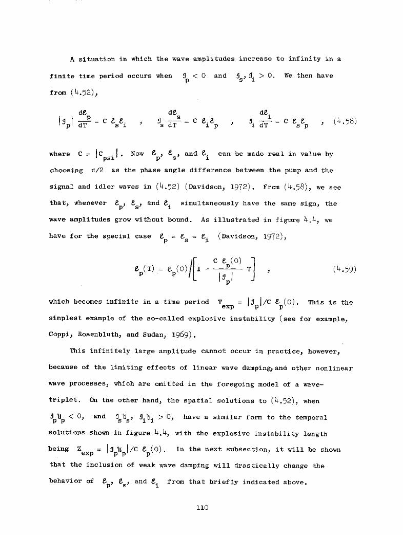
A situation in which the wave amplitudes increase to infinity in a
finite time period occurs when 3 < 0 and s, . > 0. We then havep s I
from (4.52),
de de de.
p P e. s =C e. . , = C ee(4.58)p dT s I s dT I p 1 dT sp
where C =C psi. Now 8p, s) , and 6. can be made real in value by
choosing n/2 as the phase angle difference between the pump and the
signal and idler waves in (4.r2) (Davidson, 1972). From (4.r8), we see
that, whenever p , 8&, and ei simultaneously have the same sign, the
wave amplitudes grow without bound. As illustrated in figure 4.4, we
have for the special case 8 = s = _ (Davidson, 1972),p s 1
ep(T) = p() p T] (4.r9)p p p
which becomes infinite in a time period Tex p = 1 /C e (0). This is the
simplest example of the so-called explosive instability (see for example,
Coppi, Rosenbluth. and Sudan, 1969).
This infinitely large amplitude cannot occur in practice, however,
because of the limiting effects of linear wave dampingand other nonlinear
wave processes, which are omitted in the foregoing model of a wave-
triplet. On the other hand, the spatial solutions to (4.52), when
5 p < 0, and Is 1i i > O, have a similar form to the temporal
solutions shown in figure 4.4, with the explosive instability length
being Zexp = 131 p/C ep (0). In the next subsection, it will be shown
that the inclusion of weak wave damping will drastically change the
behavior of p, , and ,i from that briefly indicated above.
110

I~pI
I-
ST (or Zp) T(or Z)Texp(Or Zexp)
Figure 4.4 The behavior of J in the explosive instability of
three-wave interaction, occurring when jp is different
in sign from Is and 9i for their temporal solutions,
or 9j lp is different in sign from jss and '9. .
for their spatial solutions.
111
4.4.2 Wave Damping
The effects of weak linear wave damping can be included phenomenolo-
gically in the coupled mode equations (4.52) (Sj8lund and Stenflo, 1967),
+ + e = -c e.+p axp psi s i
+ s *- + F = C 8.8s (T s SX s s psi g p
i\aT i aX i i -psi sp
where the rp,s,i represent the normalized damping rates of the pump,
signal, and idler. Due to the presence of rp . , le p must be larger
than some threshold before es and P. can be amplified. This threshold
field, eth for amplification can be obtained by setting /T = = 0= /aX in
the last two expressions of (4.60). We then obtain
th (4.61)ICpsiI
after cancelling es and .. When the pump field is not far above the
threshold, we may obtain the initial parametric amplification rate for
waves propagating parallel to Z, in a fashion similar to that used in
obtaining (4.54) (Louisell, 1960), as
2 22 KO th
K+ (4.62)s i+
where Kg is given by (4.54); ps, i" and Kth are defined by
112
s i = Ko , (4.63)s i = e
p th
2 2and we have assumed (s + i ) >> 4( K th
For the case of a large amplitude undamped pump wave, the spatial
solutions for linearly damped signal and idler waves have already been
presented in the context of nonlinear optics (Bloembergen, 1965; Bobroff,
1965). The stability analysis, in line with the approach by Harker and
Crawford (1969a) and Van Hoven (1971), has been extended to this case by
Bers, Chambers, and Hawryluk (1973). Here, we wish to extend the analysis
to account for a damped pump wave. A similar problem has been studied
by Ohnuma and Hatta (1970), and by Porkolab and Chang (1970).
By making the phase of t different from those of s and Pi by
n/2 in (4.60), we have for the one-dimensional case (Davidson, 1972),
s sdZ + sI cs (4.64)U ( ) = C &i p i i i i = C s ( .
where C = ICpsil; ep, es, and ei are real in value, and we assume an
exponentially decaying, large amplitude pump wave
?P= p(0)exp(-t Z) (le >> JjeI) (4.6))
Case 1. p i 4s = pi = p.: The simplified case where 4p = ks= i=
has been treated by Ohnuma and Hatta (1970), and a further simplifi'cation
to second harmonic generation by a large amplitude ion-acoustic wave has
been studied by them and by Litzenberger, et al. (1972). For purposes
of comparison between theory and experiment in Section 5.2.3, we shall
113

consider solutions for parametric amplification when 4. p p.s = p = 4.
We then have as solutions of (4.64) , for the case of co-flow (figure 4.2a)
es = [s() cosh M + i(0)i1-s s sinh M exp(-pZ)
=i 8i(0) cosh M + es(0)(si ) sinh M exp(-pZ)
F CS (0) e(o)M(Z)=ML- exp(-Z) , MO) 1/2 (4.66)
p (U11ssi .i) 1/2 th p
where Ps(0) and e.(0) are the values of es and e at Z = 0, and
the second expression for M0 is obtained by using (4.61).
By evaluating ds/dZ and dSi/dZ at Z = 0, we find that es
and 8i grow in the vicinity of Z = 0 according to (4.61) and (4.62).
For Z such that p Z >> i, PS and e both decay by linear damping.
This behavior is illustrated in figure 4.5 and is drastically different
from that shown in figure 4.3 where damping was not included. In the simpler
theoretical model used by Ohnuma and Hatta (1970), in which 4p = p., the
following assumptions were made,
M(Z) << 1 , es(0) > 1 j- , (4.67)() M0 (i/s
where the second condition is obtained by making de./dZ > 0 at Z = 01
according to the second expression of (4.66). It then follows that F.1
has its maximum value at ZO = in2/p 0 .7/p, a result obtained
without assuming 4p = p.
114

S
0 Zo Z
Figure 4.5 The schematic behavior of Ps and i according
to (4.66), where wave damping of 8p, 8s, and 8i
has been included. When p = p, and under the
condition (4.67), the peak location Z0 of 8i
becomes independent of p (0).

Case 2. p / p. p. : The solutions for s and e. must now be
expressed in terms of Bessel functions (Porkolab and Chang, 1970). We
shall consider only the case where p > 0 (Ip > 0), .s < 0 (Us < 0),
and pi > 0 ('Ui > 0), i.e. the contra-flow or back scatter case (Barnes,
1964; Bloembergen, 1965), as illustrated in figure 4.2b, relevant to
examples in Sections -.3.2, 5.4.3, and 5.5.4. Under these conditions the
solutions of (4.64) for 8s and 6i can be written as5. 1
= [Cl Jv (X) + C p N,,1 (X) exp[-(4p+ +p +i z1
s = [Csl Jv(X) C N(X) exp[-( p + (ps i(4.68)
where the quantities X, v, IMOI Cil,2 and Csl,2 are defined by
X = M01 exp-pZ v= - - - p5
IM01= C (0) (0s 1s -/2p (ru I .)th p
Cil = I2 NIv-1(MO s1 2 (0) - N( I0 ) (0)
Ci2 [v 0/ i) - s V, 2 -1 (vlIMO i s(O
C 1 IMO s 1/2
Cs1 TM I [N v-1 (IMO (0) -) I N 11 M I (0
T IMO j 111(I j s 1l/2 ( (I o 1Cs2 = 2 [ is sJ v\O' i(0 - Jv-l\ s0 ,0 (4.69)
116

where J (X) and N (X) are Bessel functions of the first and second
kinds (Abramovitz and Stegun, 1965).
Simplifications of (4.68) are possible under various conditions of
interest for Section 5:
X << : In this case, 8i and 8s reduce to
si i
X exp [ -p + IsI + ZZ (4.71i
V X: We now have for /. and the expressions
+ [ Xs(O)X2i - + (o) 1 )2 exp ( )
s e s(o) e(v-01)X M
X exp [(4 p + s + (4.70)
where X i and X are defined by
117117
where X2i and X2s are defined by
IMQO ss1/2 MO s 1s .1/22i ' 2s 2v '. (4.73)
and e0 has been written for exp(l) = 2.718...
X > v >> 1: In this approximation, 8. and s reduce to1 s
L s ui i I $ L s if 2' s&(0)cos M + e.(o lA \1
(/2+
es [Pss(0)cos M + Pi(0( 1 ) sin M exp[- s + i (4"74)
We note that,
M(Z) = 1M [1 - exp(-pZ)] j 0 pZ , (4I71)
where the second expression for M(Z) is appropriate when p Z << 1. In
(4.70), (4.72), and (4.75), the quantity IMo0 has been defined in (4.69).
It will be seen in Section 5 that the behavior of e and e. accordingS 1
to (4.70)-(4.75) is drastically different from that indicated in
Section 4.4.1 where linear damping is neglected.
Case 3. Noncollinear Propagation: So far we have assumed that
the group velocities are collinear. In preparation for Section 5.5.4,
we now consider the case when 11 '1 , and '1 are no longer collinear.
The coupled mode equations (4.64) become
118

s x C e.ep
a 1 + r) es C Ip(.76)i xx X iz i Z 1 s p
where sx' 1sz ',ix, and 1iz are defined by
X = C sinV s ' Oz 1 cosY It. = 'U. sin, 'U . z=UicosY.,(4.77)
with Y and Y. being the angles of 't and 1i with respect to thes 1 "-'5
positive Z direction. Substituting
EP(X,Z) = es(Z) exp(-sxX ) , &(X,Z) = .i(Z) exp(-4ix) ,
s s sx 1 ix
SX - sinY 7 s = U. cosY ' COS . sinTi iz- . cosYiS S 1 1
(4.78)
(4.76) can be reduced to
S~ s - + sz) e(z) = c .(z) (z) exp[(s- )
d - i) e.(z) C (z) e exp[( - p. (4.79)S --iz dZ 1 s p .ix sx
It will be seen that, along a path with X constant, (4.79) is equivalent
to (4.64), but with different wave coupling coefficients. Along an
appropriately chosen Z-axis, where X = O, e.g. the central plane of a
plasma slab, the form of (4.79) becomes identical to that of (4.64). The
solutions, (4..68)-(4.75), become the solutions of (4.79) when Us i' 4s'
and ki are replaced by '1sz 1iz' sz' iz, respectively.
119
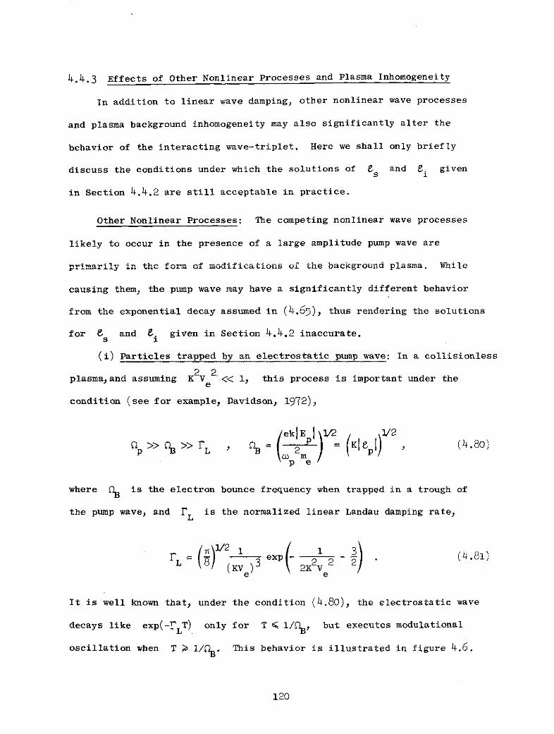
4.4.3 Effects of Other Nonlinear Processes and Plasma Inhomogeneity
In addition to linear wave damping, other nonlinear wave processes
and plasma background inhomogeneity may also significantly alter the
behavior of the interacting wave-triplet. Here we shall only briefly
discuss the conditions under which the solutions of 8 and L. givens 1
in Section 4.4.2 are still acceptable in practice.
Other Nonlinear Processes: The competing nonlinear wave processes
likely to occur in the presence of a large amplitude pump wave are
primarily in the form of modifications of the background plasma. While
causing them, the pump wave may have a significantly different behavior
from the exponential decay assumed in (4.65), thus rendering the solutions
for 8 and 8. given in Section 4.4.2 inaccurate.s 1
(i) Particles trapped by an electrostatic pump wave: In a collisionless
plasma.and assuming K 2V 2<< 1, this process is important under thee
condition (see for example, Davidson, 1972),
ek E (Klp) 2 (4.80)
Q >> >> rL 2 = K , (4.80)p e
where CB is the electron bounce frequency when trapped in a trough of
the pump wave, and FL is the normalized linear Landau damping rate,
L () 1 exp 2 - 3 (4.81)L 8 (KVe) 3 " 2K2V e2 2
It is well known that, under the condition (4.80), the electrostatic wave
decays like exp(-FLT) only for T E 1/B, but executes modulational
oscillation when T > 1/D. This behavior is illustrated in figure 4.6.
120

oC Exp (-rLT)
0 2rr 4,r 6r
,BT
Figure 4.6 The behavior of an electrostatic pump wave amplitude under
the influence of trapped electrons (-) in a collisionless
plasma under condition (4.80). In the absence of electron-
trapping, the wave decays according to linear Landau
damping as exp(-LT) (----).
121

The results of Section 4.4.2 are therefore appropriate only for T 1 1/1B,
or for Z < 1/S1p when considering spatial evolution.
The first condition in (4.80) is necessary to restrict the size of
lepl so that the electron density perturbation is much smaller than the
quiescent density (Davidson, 1972), and is consistent with the assumption
of weak perturbation used in Section 4.2 in approximating the Lagrangian.
The second condition in (4.80) is required to allow the trapped electrons
to make many bounces in a wave trough before they become untrapped due towave damnin. Therefore when +he c1o onl d -, is much larger
. ... .- - I D ILUU11 UalllrL c
than rL rc should replace PL in (4.80). Following the same reasoning,
ec should be replaced by the total measured pump wave damping rate p ,
which may be a sum of rc and the nonlinear damping rate rNL that
accounts for all the nonlinear effects on the pump wave. We then have
from (4.80),
P 1/2(4.82)
as the condition under which the trapped particle effects on an electro-
static pump wave are negligible.
(ii) Plasma heating: Substantial background modification in the
form of plasma heating by an incident wave can occur in a collisional
plasma due to collisional randomization of the ordered perturbation in
electron motion. It has been shown that the electron temperature, Te
increases from its quiescent value, T , roughly according to
(Ginzburg, 1970),
S1+ ( II 'T v , (4.83)
122
2 2 2when a >> v, pe with ve being the electron-ion and electron-neutral
energy transfer collisional frequency. When l 2 >> ~, it is seen
that the corresponding temperature increase can be substantial, thus
changing the wave coupling coefficients and linear wave properties.
Thus, in the presence of a large amplitude pump wave, the electron
temperature should be determined from (4.83) before using the results of
Section 4.4.2.
(iii) Density Modifications: Particle trapping and plasma heating
deal with the modification of the plasma background in velocity space.
Modifications in configuration space can occur when the large amplitude
wave is inhomogeneous in amplitude, as is the case in (4.69). This results
2in an equivalent potential energy, N (normalized to m c ), for each
Ne
charged particle (Ginzburg, 1970),
le I e (0)12- 2 - 2 exp(-24pZ) . (4.84)
This nonlinear effect becomes important when N is comparable with the
2average electron thermal energy, V 2/2. So the condition under which
e
the background plasma density is not significantly altered by an inhomo-
geneous large amplitude pump wave is then,
.l (2 2 2p e (4.85)
over the plasma region where aZ .1. The effects of background
inhomogeneity on the three-wave interaction process will be briefly
discussed below.
123

Plasma Inhomogeneity: The size of the plasma region, ALO, in which
nonlinear wave interaction occurs, may be limited either by boundaries
in the case of a uniform plasma, or by satisfying the synchronism condi-
tions (4.48) in the case of a slightly inhomogeneous plasma.
(i) Bounded homogeneous plasma: In this casewe require
KAL 0 >> 1 , KAO > 1 , (4.86)
to see significant nonlinear wave amplification within ALO . If there
is a departure AK (= -K'-K/) from synchronism, then the parametric
growth will be substantially unaffected only if
AK * AL < . (4.87)
This conclusion may be reached by considering the exact expression for
the integral in (4.34) (Schiff, 1970; Phelps, Van Hoven, and Rynn, 1973)
AK AK *ALOL dZ exp(iAK * Z) = 2 sin AK Lo
-L AK s a (4.88)
which has the significant value of roughly unity only when (4.87) is
satisfied. Note here that we have neglected the reflection of waves from
the boundaries.
(ii) Weakly inhomogeneous background: In this case, the quantity
AK is a function of AL, where AL is the distance from the point of
perfect synchronism. Then (4.87) can be used to determine the width,
AL0, of the region over which synchronism is sufficiently well satisfied
for parametric amplification to occur. Assuming linear dependence of AK
on AL, we then have from (4.87)
124
ALO < 1 ,/ AK = aL (4.89)
which agrees With a result by Harker and Crawford (1970).
4.5 Discussion
The purpose of this section has been to apply the macroscopic-
Lagrangian obtained in Section 3 to the description of parametric wave
amplification phenomena in a homogeneous plasma. In Section 4.2, the
Lagrangian of .(3.22) was expanded in terms of the perturbations, ~ A,
and pl, in plasma cell position x and the vector and scalar potentials
A and cp. In Section 4.3, the averaged Lagrangian) technique was applied
to obtain the energy densities and energy flux densities of the linear
waves,and the nonlinear wave coupling coefficients. We specialized in
Section 4.4 the analysis of the three-wave coupled mode equations to
parametric amplification, and demonstrated how to solve them in the presence
of linear wave damping. The results will be used in Section 5 to make
comparisons between theory and experiment.
125

r- THREE-WAVE INTERACTIONS: APPLICATIONS
5.1 Introduction
Nonlinear wave-wave interaction represents the lowest order correc-
tion to linear plasma wave theory. It must be described and understood,
together with the phenomena of nonlinear wave-particle interactions, which
have been ignored in this thesis, before effective progress can be made
towards understanding such significant plasma problems as turbulence and
anomalous transport (Kadomtsev, 1961). In view of its importance, one
would expect to find a variety of theoretical predictions for interactions
between various types of plasma waves, and a corresponding series of
experimental investigations designed to test the validity of the theory.
This desirable stage has not been reached, however. Although there
have been many analyses of wave-wave interactions, there have been few
experiments carried out to test them rigorously. A representative sample
of the literature is given in Table 5.1. The list is not intended to be
exhaustive, but illustrative. Most of the nonlinear wave coupling
coefficients have been derived by the conventional iterative method. This
approach is conceptually simple, but generally involves greater algebraic
complexity than the Lagrangian method.
Although all of those results listed could be rederived by the
averaged Lagrangian methodby use of an appropriate Lagrangian density,
only a small number of the analyses were carried out by this method.
These may be categorized by the plasma models used.
Cold Plasma: Using the cold plasma Lagrangian, Galloway and Crawford
(1970) have obtained the coupling coefficients for transverse waves
propagating at arbitrary angles to the static magnetic field. As men-
tioned in Section 4.1, a similar study has been presented by Boyd and
126

Table 5.1 Some derivations of wave coupling coefficients using (a) the
averaged Lagrangian method and (b) the iterative method, with
(c) related experimental work. The abbreviations used below
represent, C: cold plasma, M: macroscopic warm plasma, and
m: microscopic warm plasma. With respect to the static
magnetic field, we have, 11: parallel propagation, -- : quasi-
parallel propagation, 1: perpendicular propagation, and
X: oblique propagation. With respect to the directions of the
phase velocities, we have, O = 0: collinear waves,and 8 ; 0:
noncollinear waves.
Interacting Waves, References; Theoretical Assumptions
Three ion-acoustic (b) Litzenberger and Bekefi (1969); M, = 0waves (b)(c) Ohnuma and Hatta (1970); M, 8 = 0
i(b)(c) Litzenberger, Mix, and Bekefi (1972);
M, = 0
Two electron plasma (a) Suramlishvili (1964); m, a 0waves and one ion- (a) Kim (1972); M, 8 = 0acoustic wave
(b) Oraevskii and Sagdeev (1963); M, G ' 0
(b) Lee and Su (1966); M, 8 0
(b) Gratzl (1971); m, 0
Three electron plasma (a) Galloway and Kim (1971); m, 8 = 0waves (a) Kim (1972); m-, t 0
Two whistlers and one (b) Forslund, Kindel, and Lindman (1972);
ion-acoustic wave M and m, I
(b) Porkolab (1972); m, X, O 0
(c) Porkolab, Arunasalam, and Ellis (1972)
127

Table 5.1 (cont.)
Interacting Waves References; Theoretical Assumptions
One long wavelength (a) Kim (1972); Mordinary wave, one (b) Nishikawa (1968); Melectron plasma wave,and one ion-acoustic (b) Lee and Su (1966); Mwave (b) Harker (1971); M
(b) Dubois and Goldman (1965); m
(b) Silin (1965); m
(c) Stern and Tzoar (1966b)
One extraordinary (b) Porkolab (1972); m, X, 8 / 0wave, one elec-tron plasma wave,and one ion-acousticwave
One cyclotron harmonic (b) Gratzl (1971); m, X, 8 / 0wave, one or twoelectron plasma waves,and one ion-acousticwave
Two ion cyclotron, or (a) Suramlishvili (1970); m, X, V 0two Alfven waves,and one ion-acoustic (b) Lee and Kaw (1972); M, m, If
wave (b) Hollweg (1971); M, II
(c) Belcher and Davis (1971)
(c) Dubuvoi and Fedyakov (1968)
Two (or one) lower (a) Suramlishvili (1971); m, x, X 0hybrid waves andone ion cyclotron, or (b) Kindel, Okuda, and Dawson (1972);magnetosonic, wave (or m, X, 8 V 0
two ion-acoustic (b) Fidone (1973); m, X, O V 0waves) (b) Karney, Bers, and Kulp (1973); M, X, o 0
(c) Hooke and Bernarbei (1972)
128
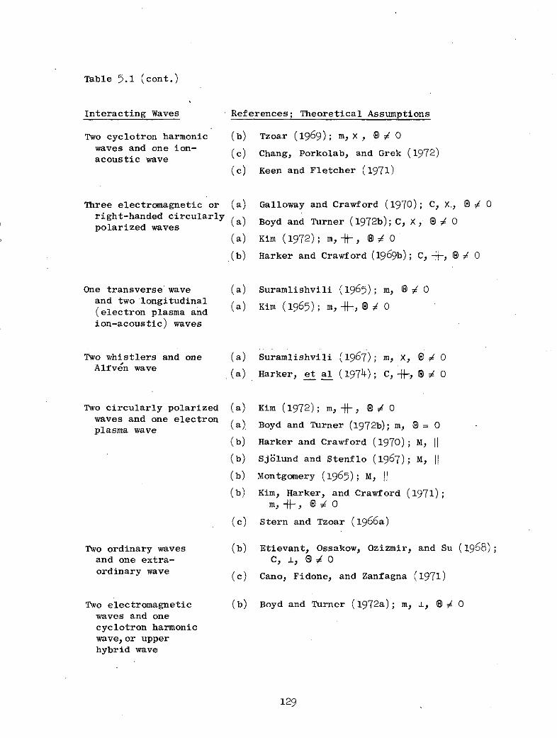
Table 5.1 (cont.)
Interacting Waves References; Theoretical Assumptions
Two cyclotron harmonic (b) Tzoar (1969); m, x , e 4 0waves and one ion- (c) Chang, Porkolab, and Grek (1972)acoustic wave
(c) Keen and Fletcher (1971)
Three electromagnetic or (a) Galloway and Crawford (1970); C, X., V 0right-handed circularly (a) Boyd and Turner (1972b); C, X, - 0polarized waves
(a) Kim (1972); m,- . 8 - 0
(b) Harker and Crawford (1969b); C, S-, O 0 O
One transverse wave (a) Suramlishvili (1965); m, -j 0and two longitudinal(electron plasma andion-acoustic) waves
Two whistlers and one (a) Suramlishvili (1967); m, X, 8 ® 0Alfv'n wave
(a) Harker, et al (1974); C, H-, S 0
Two circularly polarized (a) Kim (1972); m,0-, O Owaves and one electronwaves and one electron (a) Boyd and Turner (1972b); m, e = 0plasma wave
(b) Harker and Crawford (1970); M, II
(b) Sjblund and Stenflo (1967); M, I
(b) Montgomery (1965); M, II
(b) Kim, Harker, and Crawford (1971);m,-H-, 9V0
(c) Stern and Tzoar (196 6a)
Two ordinary waves (b) Etievant, Ossakow, Ozizmir, and Su (1968);and one extra- C, 1, ® 0
ordinary wave (c) Cano, Fidone, and Zanfagna (1971)
Two electromagnetic (b) Boyd and Turner (1972a); m, ±, 8 V 0
waves and onecyclotron harmonicwave,or upperhybrid wave
129

Table 5.1 (cont.)
Interacting Waves References; Theoretical Assumptions
Three cyclotron (a) Kim (1972); m, 1, 8 1 0
harmonic waves (b) Harker and Crawford (1968); m, A, S 1 0
(c) Porkolab and Chang (1970)
(c) Chang and Porkolab (1970)
130
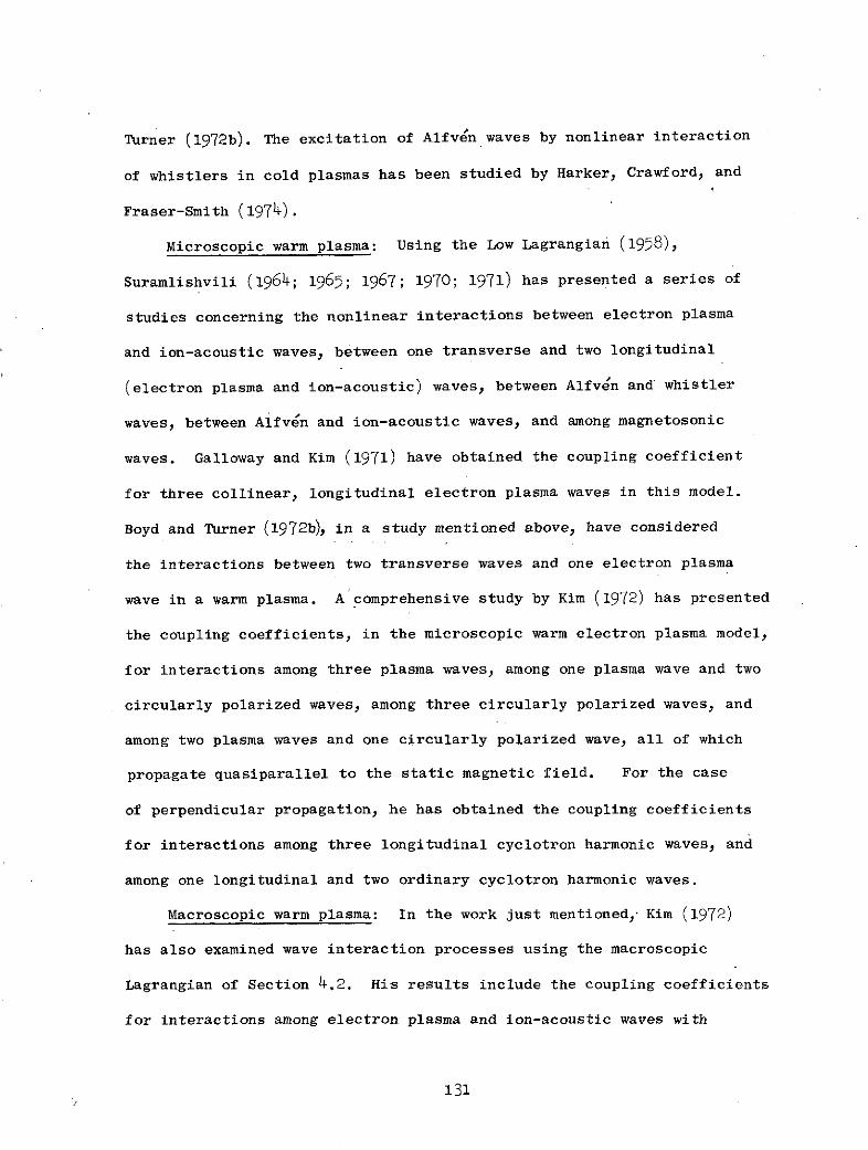
Turner (1972b). The excitation of Alfven waves by nonlinear interaction
of whistlers in cold plasmas has been studied by Harker, Crawford, and
Fraser-Smith (1974).
Microscopic warm plasma: Using the Low Lagrangian (1958),
Suramlishvili (1964; 1965; 1967; 1970; 1971) has presented a series of
studies concerning the nonlinear interactions between electron plasma
and ion-acoustic waves, between one transverse and two longitudinal
(electron plasma and ion-acoustic) waves, between Alfven and whistler
waves, between Alfvn and ion-acoustic waves, and among magnetosonic
waves. Galloway and Kim (1971) have obtained the coupling coefficient
for three collinear, longitudinal electron plasma waves in this model.
Boyd and Turner (1972b), in a study mentioned above, have considered
the interactions between two transverse waves and one electron plasma
wave in a warm plasma. A comprehensive study by Kim (1972) has presented
the coupling coefficients, in the microscopic warm electron plasma model,
for interactions among three plasma waves, among one plasma wave and two
circularly polarized waves, among three circularly polarized waves, and
among two plasma waves and one circularly polarized wave, all of which
propagate quasiparallel to the static magnetic field. For the case
of perpendicular propagation, he has obtained the coupling coefficients
for interactions among three longitudinal cyclotron harmonic waves, and
among one longitudinal and two ordinary cyclotron harmonic waves.
Macroscopic warm plasma: In the work just mentioned, Kim (1972)
has also examined wave interaction processes using the macroscopic
Lagrangian of Section 4.2. His results include the coupling coefficients
for interactions among electron plasma and ion-acoustic waves with
131

parallel propagation, and among an ordinary wave with perpendicular pro-
pagation, an electron plasma wave with quasiparallel propagation, and
an ion-acoustic wave with quasiparallel propagation.
Most theories of wave-wave interaction have been carried out assuming
the plasma to be homogeneous. In the experiments with which they have
been compared, the plasmas have often been strongly inhomogeneous,
rendering the wavenumber synchronism condition (4.48) difficult to
realize experimentally. In these cases, comparison between theory and
experiment will be impossible, unless the theory is improved by taking
background inhomogeneity into account (Kino, 1960; Larsen, 1972). In
mitigation, it should be pointed out that many of the experiments were
aimed at studying the anomalous absorption of large amplitude waves, and
the subsequent heating of the plasma (Porkolab, et al.,1972; Stern and
Tzoar, 1966b; Dubuvoi and Fedyakov, 1968; Hooke and Bernarbei, 1972; Chang,
et al. 1972; Keen and Fletcher, 1971), rather than to produce ideal
conditions for testing basic plasma theory.
Some experiments have, however, been carried out in effectively
homogeneous plasmas with synchronism in both frequency and wavenumber
realized. In particular, second harmonic generation caused by an ion-
acoustic wave propagating along a plasma column have been observed by
Litzenberger, et al.(1972). Three interacting ion-acoustic waves have
been studied by Ohnuma and Hatta (1970). Three interacting cyclotron
harmonic waves have been studied by Chang and Porkolab (1970). Parametric
excitation of ion-acoustic waves by whistler waves has been observed
by Porkolab, et al.(1972). To explain the observed wave behavior, it
was found necessary to include the effects of wave damping. With the
132

exception of the case for harmonic generation by ion-acoustic waves
(Litzenberger et al., 1972), only qualitative agreement between the
solutions of the coupled mode equation and the waves observed has been
achieved (Ohnuma and Hatta, 1970; Chang and Porkolab, 1970; Porkolab,
et al., 1972). The purpose of this section, then, is to establish
more nearly complete quantitative comparisons between some of these
experiments and the theory developed in Section 4.
In this section we shall specialize the general results of Section 4
to two experimental situations. The first will be that of Ohnuma and
Hatta (1970), for which we shall consider the collinear excitation of an
ion-acoustic wave by two other ion-acoustic waves (Section 5.2), and by
two longitudinal electron plasma waves (Section 5.3). The second will
be that of Porkolab, et al.(1972), for which we shall consider the exci-
tation of a collinear (Section ;.4),and a noncollinear (Section ".5),ion-
acoustic wave by a large amplitude whistler.
5.2 Nonlinear Interaction of Ion-Acoustic Waves
..2.1 The Experiment and Interpretation
The experimental set-up used by Ohnuma and Hatta (1970) is shown
schematically in figure 5.1. Their plasma had the typical parameters:
n n. 1 109/cm , T 5 10 4 oK , Ti 3000 Ke 1 e 1
P 9 mTorr v 4.6 X 10sec , . . 3.0 X 10/sec , (5.1en in
where the effective electron- and ion-neutral momentum transfer collision
frequencies have been calculated from (Ginzburg, 1970)
133
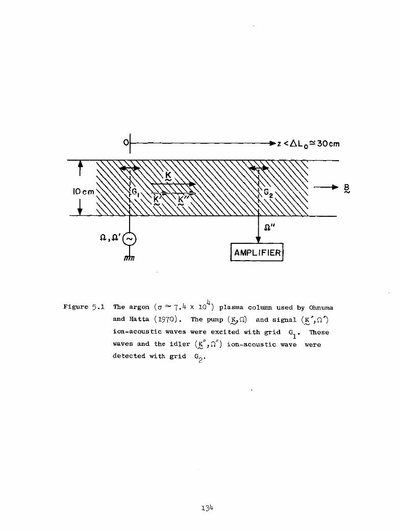
oj > z <ALo, 30cm
10 cmK\
AMPLIFIER
Figure 5.1 The argon (a 7.4 10 4 ) plasma column used by Ohnuma
and Hatta (1970). The pump (b Q) and signal (K , ')
ion-acoustic waves were excited with grid G . These
waves and the idler (K , ,Q) ion-acoustic wave were
detected with grid G2.
134
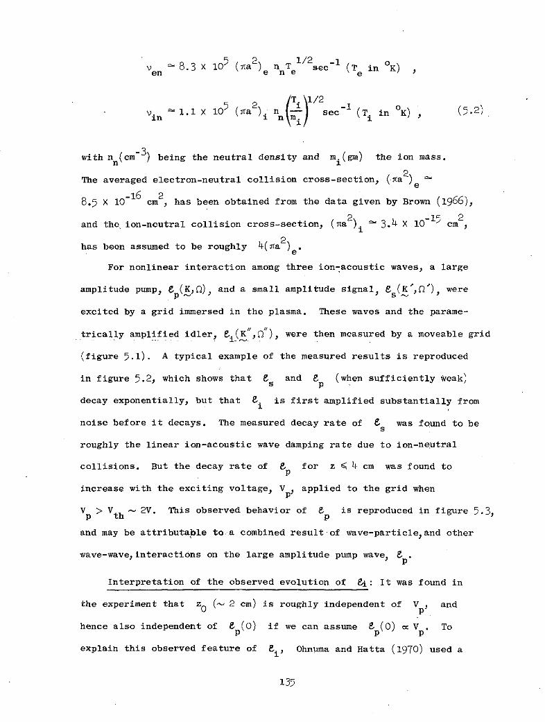
P 2 c1/2 -Ven 8.3 x 10 (a )e n e sec (T e in K)
v. 1.1 X 10 (a2 n -31- sec -1(T. in OK) (;.2)in iln )
with n (cm-3) being the neutral density and m.(gm) the ion mass.
The averaged electron-neutral collision cross-section, (Ta 2)e
8.5 X 1016 cm , has been obtained from the data given by Brown (1966),
and the ion-neutral collision cross-section, (Ta2).i 3.4 X 10⁻¹ cm
has been assumed to be roughly 4(3a 2 ) e
For nonlinear interaction among three ion-acoustic waves, a large
amplitude pump, ep(KD), and a small amplitude signal, es (K',D) were
excited by a grid immersed in the plasma. These waves and the parame-
trically amplified idler, 8i(K ",2), were then measured by a moveable grid
(figure 5.1). A typical example of the measured results is reproduced
in figure 5.2, which shows that 8 and 8 (when sufficiently Weak)s p
decay exponentially, but that 8. is first amplified substantially from1
noise before it decays. The measured decay rate of es was found to be
roughly the linear ion-acoustic wave damping rate due to ion-neutral
collisions. But the decay rate of 8 for z 4 4 cm was found top
increase with the exciting voltage, Vp, applied to the grid when
Vp > Vth - 2V. This observed behavior of Fp is reproduced in figure 5.3,
and may be attributable to a combined result of wave-particle,and other
wave-wave, interactions on the large amplitude pump wave, 8p.
Interpretation of the observed evolution of ei: It was found in
the experiment that z0 (- 2 cm) is roughly independent of Vp , and
hence also independent of 8p () if we can assume P. (0) = V . To
explain this observed feature of ei, Ohnuma and Hatta (1970) used a
135

S E (120kHz)kHz)
I, I
W
0D 8 (I2OkHz)
LJI-
-J
-J
CIC 0 -(80 kHz)
IZo Z0 I ~I I I0 2 z 0 4 6 8
z (cm)
Figure 5.2 A typical observation by Ohnuma and Hatta (1970) of inter-
action among collinear ion-acoustic waves. The exciting
grid for the pump, 6 , and signal, es, is located at
z = 0. The peak of the idler, 8i, is located at z0 .
136

Ep(200 kHz)
S 2
A A
V 15V
-10 \A\ o
>
\\ 5
I-I1O E
I I
0 4 8z (cm)
Figure 5.3 The measured behavior of ap for several exciting voltages,
V p at the grid. For z 4 4 cm, the spatial decay rate,
p4 of 8 was found to increase with V whenp p p
Vp > Vth ~ 2V.[Ohnuma and Hatta (1970), figure 16].
137

set of coupled mode equations with identical wave damping rates, i.e.
Pp = s i i = ~. Assuming (4.67), they were able to show that
ZO (- 0.7/p = 0.7/) is independent of 8 (0), as was shown in the
paragraph containing (4.67) in Section 4.4.2.
As indicated in figure 5.3, however, 4p increases substantially
with p (0) [assuming p (0) = V p]. Therefore, the theoretical behavior
of 8i is more suitably described by assuming pp f .s = p.i = p. in
the coupled mode equations (4.64), whose solutions for this case are given
by (4.66). Furthermore, because e8 is damped nonlinearly, it is
reasonable to assume that p (0) > eth. Thenfrom (4.66), we have
_ (o).M(Zo) M e p 1 (. 3)0 0 th
p
showing that the first condition of (4.67) fails. Therefore, the apparent
independence of ZO in P (0) was not satisfactorily explained by the
formula Zg 0.7/ p.
Since we can only assume es(0) >> ei(0), use of (4.66) then shows
that ZO should satisfy
exp(-pZ 0 ) Z O tanh MO[ - exp(- (.4)
To determine ZO from (0.4), it is necessary to evaluate p, and
evaluate M 0 and 4p as functions of e (0)/Sth. This calls for the
examination of the linear properties and the nonlinear coupling coeffi-
cient of the ion-acoustic waves.
138

5.2.2 Ion-Acoustic Waves (I) and Coupling Coefficient: 0 = 0
In this case we have K = Ki , where i is the unit vector in
the positive z direction, along which the static magnetic field is
directed. The polarization constant, M , of (4.40) then reduces to
-itMs Ms 1 s 1 s s* s
M M M M = Msxx yy 2_ 2 zz D xy yx Q 2 2
5s s
Ms = = M == M s * 0 , D = 2-Y V 2K 2(5.5)xz zx yz zy s ss z
For the experiment, we can assume
2 V 2 V 2V >> CV (T >> T) V << 1 , (.6)e i e e z
-3where the second condition follows because V 2.9 X 10 from (5.1),
e
and Kz - 50 for a typical experiment wavelength of 0.21 cm.
Under the assumption of a low frequency longitudinal wave,
e = 10,0,13 , «<<1 , (57)
the approximate ion-acoustic wave (I) dispersion relation can be obtained
by using (5.5) and (5.6) in (4.42) and (4.43). For V K << 1, it ise z
02 V 2K 2 1 V 2a z a a ee
where V is the ion-acoustic speed. As illustrated in figure 5.4, thea
wave coupling synchronism conditions are automatically satisfied over the
linear portion represented by (5.8).
139
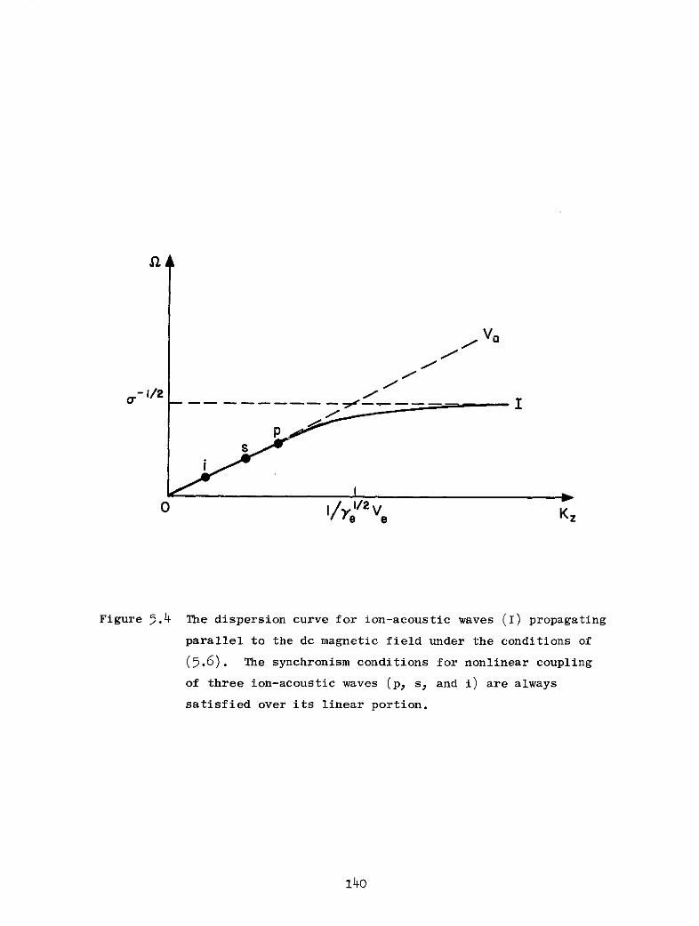
i
- 1 /2 VK
Figure 5.4 The dispersion curve for ion-acoustic waves (I) propagating
parallel to the dc magnetic field under the conditions of
(5.6). The synchronism conditions for nonlinear coupling
of three ion-acoustic waves (p, s, and i) are always
satisfied over its linear portion.
140
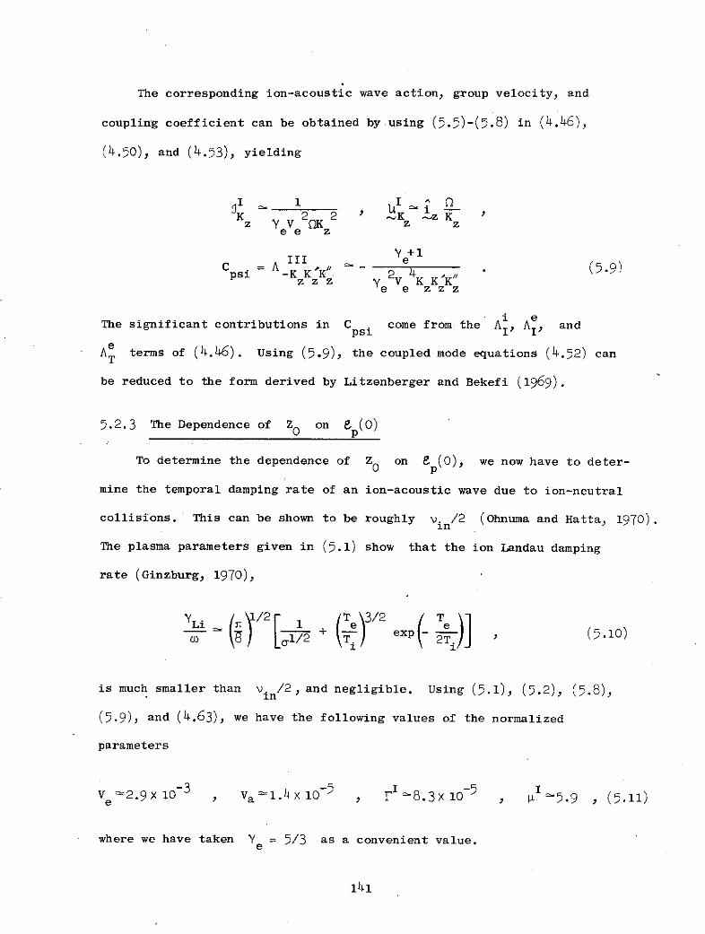
The corresponding ion-acoustic wave action, group velocity, and
coupling coefficient can be obtained by.using (5.5)-(58) in (4.46),
(4.50), and (4.53), yielding
I 1 I ^0
K 2 2 ' K -Z K zz YV OK z z
ee z
y +1III e
C = A - e (R 9 )psi -K K 2 459)z z z y V K K K"
ze e zzz
i eThe significant contributions in Cp. come from the Al, A~, and
psi I Ie
AT terms of (4.46). Using (5.9), the coupled mode equations (4.52) can
be reduced to the form derived by Litzenberger and Bekefi (1969).
5.2.3 The Dependence of ZO on 8 (0)
To determine the dependence of ZO on e (0), we now have to deter-
mine the temporal damping rate of an ion-acoustic wave due to ion-neutral
collisions. This can be shown to be roughly vin/ 2 (Ohnuma and Hatta, 1970).
The plasma parameters given in (5.1) show that the ion Landau damping
rate (Ginzburg, 1970),
yL /2 (T /2 TS+ - exp (e 10)
l[l 1
is much smaller than v. /2, and negligible. Using (5.1), (5.2), (5.8),in
(5.9), and (4.63), we have the following values of the normalized
parameters
V e 2.9X 3 Va l.4 X 0- , ~ 8.3X 10⁵ , .9 , (5.11)
where we have taken Y = 5/3 as a convenient value.
141

It remains to obtain the dependence of p /p and M 0 on 8 (0)/Sth
From figure 5.3, we first plot the corresponding values of p /p and the
pump wave exciting voltage, Vp, as shown in figure 5.5(a). Assuming
e (0) Vp, figure 5.5(a) indicates the approximate relations between
1p/p and 8p(0)/Sth, and MO and p/p4,
0.23-- + 0.77 , MO 4.3 - 3 .3 - , (5.12). th p
where the second relation has been obtained from (4.66) by use of the
first relation. Combination of (5.12) with (5.4) then determines the
dependence of ZO on ep (0)/eth, which is as shown in figure 5.5(b).
It is seen that z0 (- 2.5 cm) is in good agreement with the observed
value of 2 cm and its dependence on 8 (0)/8th according to (5.4) is
much weaker than that according to Z0 0.7/p , which is obtained under
the conditions (4.67) used by Ohnuma and Hatta (1970). Thus we conclude
that, for 8p () > eth' and with an externally applied signal wavees >> ~, the apparent independence of ZO from P (0) observed by
Ohnuma and Hatta is likely to be a result of the increase in 4p with
ep(0).
Finally, it is of interest to examine the magnitude of 8th for
the typical pump field strength indicated by Ohnuma and Hatta, which is
E ~ 32 V/cm, corresponding to a ratio of rf to dc charge densities of
roughly 1/20. For the typical pump and signal frequencies of 200 and
120 kHz, we have, by use of (4.30), (5.1), and (5.8),
n ' 7.0 x 10 , '" 4 .2 X 10 , K 50 , Kz 30 .(5.13)
142
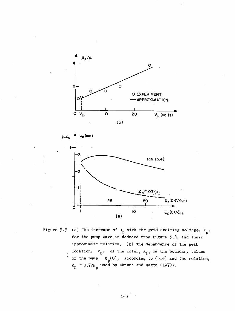
4-0
2 O
0 EXPERIMENTO - APPROXIMATIONI
0 Vth 10 20 Vp (volts)
(a)
yZ o zo(cm)
I-
-3eqn. (5.4)
2j\
25 50 Ep(O)(V/cm)
0 1I 10 Ep(O)/-th
(b)
Figure 5.5 (a) The increase of p with the grid exciting voltage, Vpp p
for the pump wave,as deduced from figure 5.3, and theirapproximate relation. (b) The dependence of the peak
location, ZO, of the idler, Fi, on the boundary values
of the pump, p (0), according to (5.4) and the relation,
ZO - 0.7/4p used by Ohnuma and Hatta (1970).
143
Then use of (4.61), (5.9), (5.11), and (5.13) gives eth 1.3 10 - 4 ,th
corresponding to a pump threshold of 4.2 V/cm. This value confirms that
the assumption p (0) > Pth in connection with (5.3) and (5.4) is
appropriate.
5.3 Excitation of an Ion-Acoustic Wave by Two Electron Plasma Waves
We will now examine the possibility of exciting an ion-acoustic wave
by two electron plasma waves in the experimental plasma discussed in
Section 5.2.1. Our purpose is to determine whether the nonlinearly excited
ion-acoustic wave should be observable under practical conditions, so that
a measurement of the coupling coefficient can be carried out.
5.3.1 Electron Plasma Waves (P) and Coupling Coefficient: e = 0
Use of (5.5) and (5.6) in (4.43) and (4.44),with the assumption of
S> 1, yields the dispersion relation for the electron plasma wave (P),
2 22 P2 1 + e = ,0, 1 . (5.14)
This P wave dispersion relation is plotted, together with that of the
ion-acoustic wave (I), in figure 5.6, which shows that the interaction
between the electron plasma (pump and signal) and ion-acoustic (idler)
waves is of the contra-flow type according to the definition shown in
figure 4 .2(b). Because the slope of the P curve at V K - 0.1 isez
much larger than Va, we have approximately K" - 2K - -2K'.z z z
The electron plasma wave action and group velocity can be obtained
by using (5.5), (5.6), and (5.14) in (4.50), giving
SP Ky z
K z ee - " (5.15)z z
144

/Ye/ \
( ZKV-'
Figure 5.6 Dispersion curves and synchronism conditions for longitu-
dinal electron plasma (pump and signal) waves (P) and
ion-acoustic (idler) waves (I).
145

The coupling coefficient can be obtained by using (5.5)-(so8) and (5.14)
in (4.46) and (4.53), yielding
C A PPI 1psi -K K'K" 2 .16)
z zz Y V Kee z
Equations (5.15) and (5.16) may be used in (4.54) to obtain the temporal
amplification rate, F0, for the ion-acoustic wave as
T, 2 , p
0 2' vee
which agrees with the result given by Kadomtsev (1965), who considered
the case Y = 1.e
5.3.2 Evolution of Fi and es
As an example, let us consider an ion-acoustic wave excited with
frequency 400 kHz and wavelength 1.1 cm, so that p2" 1.4 X 10- 3 and
K z 100. The corresponding pump wave number is then K 50. TheZ z
Landau damping rate, 'L pe for this electron plasma pump wave can then
be obtained from (4.81). It shows that I'ape is much smaller than the
damping rate due to electron-neutral collisions, ven/2, whose value is
given by (5.2) (Ginzburg, 1970). Thus we have TP 1.3 10 - 2 . By use
of this result,and (4.63), (4.61), (5.9), (5.15), and (5.16), the para-
meters in (4.68) and (4.69) take the values
p s 21 i .9 Z < 1.8 = 1.1
Pth 2.1 X 10 M01 2.1 10-2- - o. . (-.18)
146
Since X < 1M0o << 1, the approximate solution of (4.70) can be used.
When (5.18) is substituted, (4.70) becomes
t. - (0) [exp(-2.1Z) - 10-3exp(2.1Z) + 0.021 e(0)sinh(2.1Z) exp(-3Z) ,
e +s(O)exp(23Z) - 0.0019 ei(O)sinh(23Z) exp(-3Z) (5.19)
-4where we have assumed & (0) - 5.8 x 10 , corresponding to a field
p
strength of 17 V/cm.
The idler equation in (5.19) shows that if es(0) < 50 &in where
S(0) = 8in is the thermal noise level for some acceptable measuring
frequency bandwidth, no observable 8i(Z) above 8in is possible.
Assuming a measurement bandwidth of 2 kHz, the thermal fluctuations in
the electric field of the ion-acoustic wave branch may be estimated roughly
-4to be 1.5 X 10 V/cm near 400 kHz (Bekefi, 1966). To excite ei to
above this level near Z 0.2, i.e. 3.5 cm from the pump sourcewith a
-717 V/cm pump field, will require that 8(0) > 2.5 X 10⁻⁷, corresponding
to a signal field strength of 7.5 mV/cm. According to the signal equation
in (5.19), this requirement is equivalent to having es(0.3) > 10 , i.e.
injecting a 3 V/cm contra-flow signal wave at z 5 cm.
It remains to determine whether these parameters represent an acceptable
experiment to demonstrate the interaction between collinear electron plasma
and ion-acoustic waves. According to (4.82), the condition to allow trapped
-6electron effects on the pump wave to be neglected is 8 3.4x 10⁶. Fromp.
(4.83), the condition to allow electron heating effects due to the pump
wave to be neglected is ep - 2.6 X 10 - 5 . Also, from (4.85), the
147

plasma will not become significantly inhomogeneous due to spatial variation
-3of the pump wave amplitude, provided that a < V - 2.9 X 10 . Withp e
-kthe value of p - 5 X 10 , it is seen that, first, the assumption
8p = exp(-i4 Z) is inappropriate because of the trapped-particle effects,
thus rendering (5.19) also inappropriate, and second, according to (4.83),
the background electron temperature may become roughly 100 times the
value given in (5.1) when the pump wave is injected, thus significantly
changing the linear wave properties and nonlinear coupling coefficient
used in this subsection. Also, due to the temperature incrase, the
thermal fluctuations in the ion-acoustic wave branch may become much
stronger than the previously indicated value of 1.5 X 10⁻⁴ V/cm. As a
result, we conclude that it will be difficult to demonstrate the interaction
between electron plasma and ion-acoustic waves in the experimental plasma
defined in Section 5.2.1.
5.4 Excitation of an Ion-Acoustic Wave by Two Whistlers; CollinearPropagation
This nonlinear process has been observed in an experiment by Porkolab,
Arunasalam, and Ellis (1972). A detailed quantitative comparison between
the theoretical results of Section 4 and the observed parametric amplifi-
cation process in this experiment will be given here. It will be shown
that there is wide disagreement between theory and experiment. The compari-
son will suggest that important factors were overlooked in the theoretical
model, and indicate possible directions in which the theory might be
improved.
148
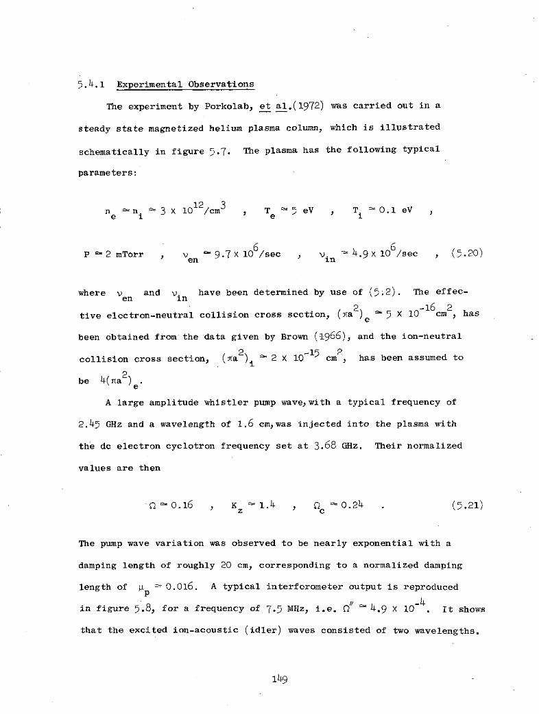
5.4.1 Experimental Observations
The experiment by Porkolab, et al.(1972) was carried out in a
steady state magnetized helium plasma column, which is illustrated
schematically in figure 5.7. The plasma has the following typical
parameters:
n n 3 X 10 12/cm T eV , T. - 0.1 eVe 1 e 1
P 2 mTorr en 9.7 X 10 6 /sec v. 4.9 10 /sec , (5.20)en 9in
where v and v. have been determined by use of (:.2). The effec-en in
(a2 10-16 2tive electron-neutral collision cross section, (a ) e 5 X 10 cm has
been obtained from the data given by Brown (1966), and the ion-neutral
collision cross section, (a2)i. 2 X 1015cm has been
be 4(Ta 2 ) e
A large amplitude whistler pump wave,with a typical frequency of
2.45 GHz and a wavelength of 1.6 cmwas injected into the plasma with
the dc electron cyclotron frequency set at 3.68 GHz. Their normalized
values are then
nOo.16 , K 1.4 , O 0.24 . (5.21)z c
The pump wave variation was observed to be nearly exponential with a
damping length of roughly 20 cm, corresponding to a normalized damping
length of 4 0.016. A typical interferometer output is reproduced
• 1o_4in figure 5.8, for a frequency of 7.5 MHz, i.e. O 4.9 X 10 . It shows
that the excited ion-acoustic (idler) waves consisted of two wavelengths.
149

01 <&L o 3m
I
c K
Figure 5.7 The experimental set-up used by Porkolab, et al.(1972),
in which ion-acoustic (idler) waves parametrically ex-
cited by whistler (pump) waves were observed. The pump wave
(K,O) was injected into the magnetized plasma column by a
slow wave structure (SWS). The spatial behavior of the idler
wave (K","Y') was measured by use of two rf probes (Pl1 and P2),narrow-band-pass filters (F), and an interferometer (Int.).
150

LaI-
0 2 4 6AXIAL POSITION z(cm)
Figure 5.8 The interferometer output showing the ion-acoustic1-4
(idler) waves at 7.5 MHz, i.e. 0" a 4.9 X 10
obtained by Porkolab, et al. (1972). The approxi-
mate behavior of the longer wavelength idler wave
for z 4 2 cm is shown dashed, and was obtained
by subtracting the shorter wavelength idler wave
from the trace.
151
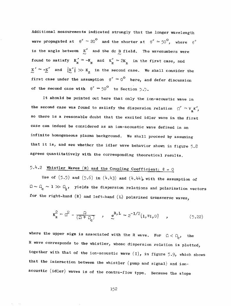
Additional measurements indicated strongly that the longer wavelength
wave propagated at 90 200 and the shorter at 0 # 500, where 8"
is the angle between K# and the dc B field. The wavenumbers were
found to satisfy K' -K and Kf 2K in the first case, andz z z z
K -K / and IK"I >> K in the second case. We shall consider the
first case under the assumption 0# 0o here, and defer discussion
of the second case with 8" 500 to Section 5.5.
It should be pointed out here that only the ion-acoustic wave in
the second case was found to satisfy the dispersion relation O p V K1a -7
so there is a reasonable doubt that the excited idler wave in the first
case can indeed be considered as an ion-acoustic wave defined in an
infinite homogeneous plasma background. We shall proceed by assuming
that it is, and see whether the idler wave behavior shown in figure 5.8
agrees quantitatively with the corresponding theoretical results.
5.4.2 Whistler Waves (R) and the Coupling Coefficient: e = 0
Use of (5.5) and (.6) in (4.43) and (4.44), with the assumption of
2- c 1 >> i., yields the dispersion relations and polarization vectors
for the right-hand (R) and left-hand (L) polarized transverse waves,
2 2 _ eR, L -1/2z ( ) e 2 1i,0} , .22)
where the upper sign is associated with the R wave. For < c, the
R wave corresponds to the whistler, whose dispersion relation is plotted,
together with that of the ion-acoustic wave (I), in figure 5.9, which shows
that the interaction between the whistler (pump and signal) and ion-
acoustic (idler) waves is of the contra-flow type. Because the slope
152

S
Kz
Figure 5.9 Dispersion curves and synchronism conditions for
whistler (pump and signal) waves (R) and ion-
acoustic (idler) waves (I).
153

of the R curve at Kz " 1.4 is much larger than Va) we have approximately
K// 2K -2K'. Since this condition was observed experimentally, thez z z
collinear approximation to the wave interaction process is seen to be
appropriate.
The whistler wave action and group velocity can be obtained by using
(5.5), (5.6), and (5.22) in (4.50), giving
2R 1 z 1 z (-.2)9 + +K 2 2 2 ' rz 2 2
The coupling coefficient can be obtained by using (5.5)-(5.8) and (7.22)
in (4.46) and (4.53), yielding
C cRRI ALRI 1 z z .24)psi K K K KKK 2K 2 n (5.24)z z z zz yV Ke e z c
where we have used the relation, R = . In this expression, thei!!K K
factor 1/y V K2 is due to the factor 1/D in M e of (5.5). Ifeez e zz
the ion-acoustic wave (I) were replaced by an electron plasma wave (P),
this denominator would be replaced by 2 - Y V2K 2 2 1, by useee z
of (5.5) and (5.6). The resulting coupling coefficient, AK K "' is
then identical to that obtained by Harker and Crawford (1970) for the
interaction between two right-hand polarized waves and an electron
plasma wave.
5.4.3 Evolution of 8. and P_1 s
To determine the behavior of -., we need to obtain the whistler
and the ion-acoustic wave damping rates. The whistler wave is damped by
electron-neutral collisions (Fc) and, and by cyclotron resonance (rr) when
154
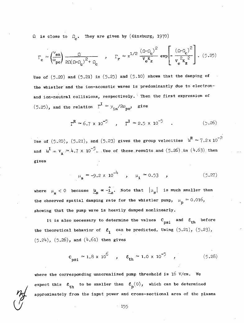
Q is close to 0 . They are given by (Ginzburg, 1970)c
1/2 c )2pe) 2D(- Vc)2 exp - ( . (.2
c/c Oce z Ve2Kz (
Use of (5.20) and (5.21) in (5.25) and (5.10) shows that the damping of
the whistler and the ion-acoustic waves is predominantly due to electron-
and ion-neutral collisions, respectively. Then the first expression of
(5.25), and the relation I in/aope give
IR =6.7 X 10- 5 r 2.5 x 10 . (5.26)
Use of (5.20), (5.21), and (5.23) gives the group velocities 1R 7.2x 10⁻²
and U -= V 4.7 X 10-'. Use of these results and (5.26) in (4.63) thena
gives
-4ts -9.2 X 10 0.53 (5.27)
where < O0 because U -i . Note that s is much smaller than
the observed spatial damping rate for the whistler pump, tp 0.016,
showing that the pump wave is heavily damped nonlinearly.
It is also necessary to determine the values Cps i and Eth before
the theoretical behavior of i. can be predicted. Using (5.21), (5.23),
(5.24), (5.26), and (4.61) then gives
6 -C. 1.8 X 10 8 1.0 X 10 , (5.28)
psi th
where the corresponding unnormalized pump threshold is 16 V/cm. We
expect this eth to be smaller than ep(0), which can be determined
approximately from the input power and cross-sectional area of the plasma
155
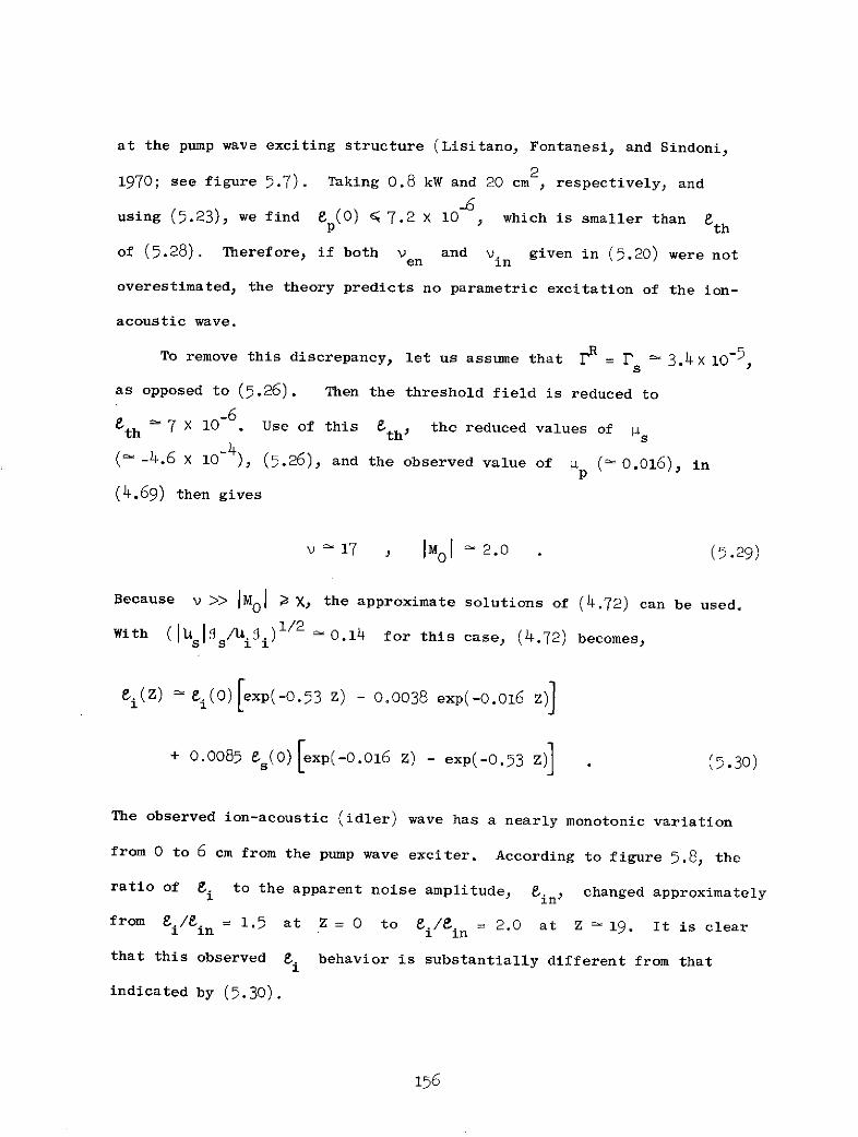
at the pump wave exciting structure (Lisitano, Fontanesi, and Sindoni,
1970; see figure 5.7). Taking 0.8 kW and 20 cm 2, respectively, and
-6using (5.23), we find 8 (0) 7.2 X 10 , which is smaller than eth
of (5.28). Therefore, if both v and v. given in (5.20) were noten in
overestimated, the theory predicts no parametric excitation of the ion-
acoustic wave.
To remove this discrepancy, let us assume that r = rs 3.4 x 10⁻⁵,
as opposed to (5.26). Then the threshold field is reduced to
66eth 7 X 10- Use of this eth' the reduced values of 4s-4
(- -4.6 x 10 ), (5.26), and the observed value of k (- 0.016), in
(4.69) then gives
v 17 , IM0 1 2.0 (5.29)
Because v >> IMO I X, the approximate solutions of (4.72) can be used.
With (ll U1s/1ii) 1/2 ' 0.14 for this case, (4.72) becomes,
ei(z) e'i(0)[exp(-0.53 Z) - 0.0038 exp(-0.016 Z)
+ o.008s es(0) [exp(-0.0l6 Z) - exp(-0.53 Z)] (5.30)
The observed ion-acoustic (idler) wave has a nearly monotonic variation
from 0 to 6 cm from the pump wave exciter. According to figure 5.8, the
ratio of ei to the apparent noise amplitude, in, changed approximately
from ./ in = 1.5 at Z = 0 to /i .in = 2.0 at Z 19. It is clear
that this observed i behavior is substantially different from that
indicated by (5.30).
156

The discrepancy between theory and experiment for this case may be
due to the effects of the finite plasma column size, the noncollinear wave
propagation (i.e. 0" 200), and some other nonlinear processes, which
were neglected in the foregoing theoretical model. In a more realistic
model, the parameters used in (4.68) and (4.69) may be modified by these
effects. It will be noted, in particular, that because i > > p > > Is
in the case of interest here, 8e(Z ) depends most strongly on 4i
(through v). If we reduce FL i by a factor of 4 from (5.27) to 4 .~0.13
and fi 0.6 x 10²F, with s (s -4.6 x 10⁻⁴ ) already reduced by a
factor of 2, then we have E (0) 28eth, V , 4.7, and IMo0 2.0. Using
these parameters, (4.72) can be used to estimate 8. and 8 as1 S
Pi(z i(0)l exp(-0.13 z) - 0.061 exp(-0.016 z)
+ 0.038 s(0) [exp(-0.016 Z)- exp(-0.13 z)
-4es(Z) - es()exp(4. 6 X 10 Zloz) (5.31)
Equation (5.31) gives a good match to the observed i with 0():8s(0):.in
given approximately as 1:80:1. It is also seen from (5.31) that for
Z t 19, we have 8 s(Z) es(0) 80 e.n. To determine if this modification
in Fi is appropriate, it would be necessary to measure es(Z)/. ins in
the corresponding experiment.
5.5 Excitation of an Ion-Acoustic Wave by Two Whistlers: ObliquePropagation
In Section 5.4 it was shown that the observed behavior of the idler
ion-acoustic wave with wavelength 0.8 cm does not correspond to the
collinear three-wave interaction theory in an infinite homogeneous plasma
157/

background. Here, we shall examine the theoretical behavior of e.
corresponding to the second observed idler ion-acoustic wave with
wavelength roughly equal to 0.16 cm (see figure 5.8). Typical wave-
numbers of the idler ion-acoustic and signal whistler waves were found
to be
K" 15 , ,480 , K 14 , O '2+ 52 . (.32)
Since obliquely propagating waves are involved in this wave interaction
process, the linear characteristics of these waves may be very different
from their corresponding waves with parallel propagation. Therefore, we
shall proceed with a discussion of these obliquely propagating waves.
5.5.1 Obliquely Propagating Ion-Acoustic Waves (I'), K' = (K",0,K")x y
In the hydromagnetic. region (0" << ne - 3.3 x 10 ), the linear
ion-acoustic wave dispersion properties may be significantly affected by
the presence of a sufficiently strong dc magnetic field. For the experi-
mental plasma of interest here, the Alfvn speed, V (0 1/2A I c-32.8 x 10 , is much larger than the ion-acoustic speed, V a 4.7x 10- .a
The ion-acoustic wave dispersion relation,and the polarization vector in
the hydromagnetic region, are then (Ginzburg, 1970)
2 _ 2K 202 _V K ' 2 e [0,1,0 . (5.33)
Here e" is linearly polarized perpendicular to K/ and B.
The ion-acoustic wave observed in the experiment, however, had a
frequency a" - 4.9 X 10 , and therefore does not fall into the hydro-
magnetic region. It is necessary to examine the properties of the wave
158

2 ,2 2in more detail. Under the condition (5.6), and with 2 >> >>
we have from (4.40)
i , i i, 1 i. i. -in.
M = M 1 =M , M = M 1xx yy . zz a,2 xy yx n/3
, 2 2+ 2 ee -u e u +a sinxx 2 ' yy 2 2os
c c
e 1 [2 2 2 2 2e e -iu2M a (a +tan e) (u +a xy yx Mzz 2 xy yx a c
zz t c
S e* +a2 e e -itaneM = M +a tane , M = M 2xz zx 2 ' yz zy 2(u 2
nc n q(u +a
2 2 2 2 2 b 2
Y V 2Ka2 o2 s2 2
Although a , b << 1 in (5.34), they are included because the zero order
terms are found to cancel each other in the derivation of the dispersion
relation and the polarization vector. Substitution of (5.34) in (4.42)-(4.44),
we then have
f,2 K 2 2K 2S 2 VK , e sin se"in cose" , (5.35)
(1/Va2 )-(K /VA2 ) a sine",,
revealing a nearly linearly polarized longitudinal wave since O" -15 ..1
2 2 K2 2 2 2/VThe approximation. Qf2 _ V K , is appropriate because l/V 30 K /VA.a a x A
When C << , we note that e reduces to (5.33) of the hydromagnetic
case.
We may now substitute (5.34) and (5.35) in (4.50) to obtain
S' i Va sine", 0, cos" . (.36)1 eV e2 K" K 2
159

When 0, (5.36) reduces to the corresponding expressions in (5.9).
Also, we have Y. = e since U. is parallel to KI.
5.5.2 Obliquely Propagating Whistlers (R'), K = [K, 0, KJ}
Reduced forms of the plasma polarization constant, M , can be
obtained from (5.5) by use of (5.6), and the condition 2 >> V K2ee
Sin /0 0c
M - M /1 0 (5.37)2 0 0 1-0 2 ,2
c
The dispersion relation and the polarization vector for the oblique
whistler wave may be obtained from (4.42)-(4.44) by use of (5.6), (5.37),
and the conditions Q < 0 and 02 a 2 sin4 ' << (2 -1)2cos26e (seec c
for example, Helliwell, 1965). We have
2'+ 2 cos9 2 2
K' _ i>' >
sin2 2 , Cosa + 38)sK 2tan OK2 sin KK' 2 tanV K2sine c2
R ,2When 0' 0, e' reduces to e of (5.22). Since K 2 >> 0 we~ c
have e [ sino9, 0, cose'J, which represents a linearly polarized
longitudinal wave, corresponding to a whistler wave that is near the
oblique cyclotron resonance <' - cos" (3T/2 > "> n/2).
Use of (5.37) and (5.38) in (4.50) now gives
160

22 1 + sin + ,2 os css 2(2c 2 a2 c2 'sin26 '
--_ 2 t-cose', O, sine' (5.39)S 0 O'K sine'c
Here, the second equation for ss is obtained by replacing Q" by
-C cose'(l - 1/K2 ), from (5.38), before eliminating terms involving
1/K "2 as small compared with unity. From (5.39), we see that the direc-
tion of 1 is perpendicular to K' and oriented so that Y = e - T/2.
5.5.3 Synchronism Conditions and Coupling Coefficient
Synchronism conditions: Since the signal and idler waves propagate
obliquely, the synchronism conditions become less obvious than those
cases shown in figures 5.4, 5.6, and 5.9. The synchronism conditions for
this case are shown schematically in figure 5.10. It contains the dis-
persion curve R from (5.22), for whistler waves with parallel propaga-
tion; the dispersion curve R' from (5.38), for whistler waves with
oblique propagation near e' + 520, and the dispersion curve I
from (5.35) (plotted with respect to a displaced origin O'), for ion-
acoustic waves with oblique propagation near e/" 480. Since the whistler
signal on the R curve is nearly at the oblique cyclotron resonance, we
have
0 ' Icose'l >> . (5.40)
RR"ICoupling Coefficient: To obtain the coupling coefficient, CKK'IK
LR 'I R L(4.53) shows that we have to evaluate A-KKK"' since e- e-K This
161
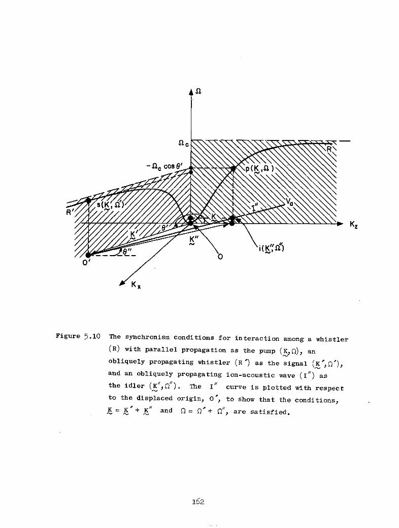
Figure 5.10 The synchronism conditions for interaction among a whistler(R) with parallel propagation as the pump (K), an
obliquely propagating whistler (R ') as the signal (K' ,O ),
and an obliquely propagating ion-acoustic wave (i) as
the idler (K",") . The I" curve is plotted with respect
to the displaced origin, 0, to show that the conditions,
162
Fiue~.0 Te ycrnimcndtosfo s(Kcinamn wite
162

requires M i and Me for a left-handed circularly polarized wave, which
can be obtained from (5.36) as
Mi = M , Me = Me ' (5.41)
Then use of (5.22), (5.34), (5.35), (5.37), (5.38), and (5.41) reduces the
LR "I'expression for AKK K from (4.46) to a simpler form. With the parameters
given in (5.20), (5.32), and (5.40), the significant terms are, in order
of ,decreasing importance
LR"I e Me e " M ee " * Me .e
S ee fS Me e") . (5.42)
The corresponding coupling coefficient, Cpsi is then
RRI" 1/2 K"sin 00 sin 2 1 RR-I 2 Ksin1 (.43)
Cpsi -KK K" Q( c -) a 2_ YeVe2K2
RR Iwhere we have made the additional simplifications to AKK RK, I appropriate
to the experimental conditions of interest, K" - K >> Kzi e -- I
Sn' >> '", and >> V e 2K/2 . The first term in the square brackets
of (5.43) is the combined contribution of the first two terms of (5.42).
Note that (5.43) cannot be reduced to (5.24), for the coupling coefficient
among whistlers and ion-acoustic waves with parallel propagation,by
making 0 = 0. This is because the polarization vector, e' in (5.38) for
the obliquely propagating whistlers, is nearly a linearly polarized longi-
tudinal wave, rather than a circularly polarized transverse wave of (5.22).
163
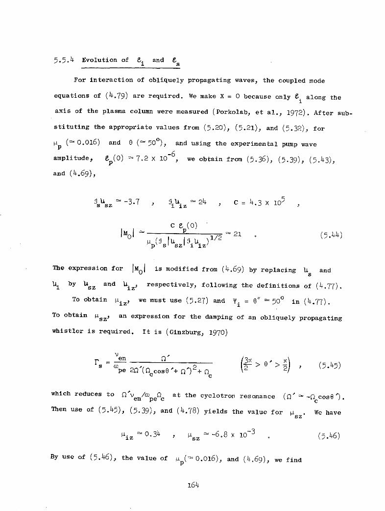
. .4 Evolution of 8. and 81 s
For interaction of obliquely propagating waves, the coupled mode
equations of (4.79) are required. We make X = 0 because only ei along the
axis of the plasma column were measured (Porkolab, et al., 1972). After sub-
stituting the appropriate values from (5.20), (5.21), and (5.32), for
4p ( 0.016) and e ( 500), and using the experimental pump wave
-6amplitude, e (0) 7.2 X 10 , we obtain from (5.36), (5.39), (5.43),
and (4.69),
s A -3.7 , 9.. -24 C = 4.3 x 10's sZ 1 iZ
M01 P2 21 (r.44)p(0 js sz 13i z
The expression for IM0 1 is modified from (4.69) by replacing 1 ands
1i by Usz and hiz. respectively, following the definitions of (4.77).
To obtain piz' we must use (5.27) and 0i = " 50 ° in (4.77).
To obtain psz' an expression for the damping of an obliquely propagating
whistler is required. It is (Ginzburg, 1970)
en (3T >_>_ _ _
pe 20 (Q cose'+ 2+c c
which reduces to 'ven /pe at the cyclotron resonance (0, -c cose ).en pe c c
Then use of (5.45), (5.39), and (4.78) yields the value for psz. We have
4iz 0.34 , sz -6.8 x 10- 3 (0.46)
By use of (5.46), the value of 4p (- 0.016), and (4.69), we find
164

1( - + 12 . (5.47)p
According to figure 5.8, we are interested in the region where z 4 2 cm,
which corresponds to Z < 5, and hence 4 Z << 1. Therefore, from
(5.44) and (5.47), we have X I M1O > v 1, so (4.74) can be used to
approximate e. and e . Substitution of (5.44), (5.46), and (5.47)1 s
in (4.74) then gives
i(z) - li(O)cos(O.34 z) + 0.39 e (O)sin(0.34 Z) exp(-0.17 Z) ,
es(Z) s(0)cos(0.34 z) - 0.39 i(0O)sin(0.34 Z)exp(-0.17 z) , (5.48)
which have been plotted in figure 5.11. Note that good agreement of e.1
with the experimental observations has been obtained without changing the
value of 4 given in (5.27). This indicates that this value of 4 i is
acceptable as the collisional damping for short wavelength ion-acoustic
waves (K" 1). For K/" 3, however, the results of Section 5.4
suggest that the long wavelength ion-acoustic wave may have been strongly
modified by those factors in the experiment not included in the wave
theory of an infinite homogeneous plasma background. Finally, to make the
agreement more satisfactory, s (Z) and P. should be measured ins in
the experiment to see whether the theoretical result in (5.48) is also
acceptable.
165

5- 0 EXPERIMENT
0 Fi/in eqn. (5.47)
T 2 3 z (cm)
5 Io-" Z
Figure '.11 Comparison between the observed evolution of the shortwavelength idler ion-acoustic wave, deduced from a result
obtained by Porkolab, et ai.(1972) (figure 5.8), and thetheoretical evolution of i(Z) according to (5.48) with
8i(0):es(0): in given approximately as 5:4:1. Thetheoretical evolution of the signal whistler wave amplitude,s (Z), is subject to future experimental verification.
166

5.6 Discussion
The verification of linear plasma wave theory imposes only the
necessity for verifying the dispersion relation, i.e. measuring
K and n. In the case of nonlinear wave-wave interaction, it is
necessary to establish not only that the linear waves satisfy the dis-
persion relation, but that also that the synchronism conditions are satisfied
and coupling coefficients follow theory. This requires more extended
series of measurements, providing details of the amplitude variations
of the pump, signal, and idler waves with distance. Few satisfying
comparisons between theory and experiment have been made so far.
We have tried to remedy this difficiency to some extent by predicting,
in Section 4, the wave amplitude behavior in space, taking into account
such practical factors as damping of the pump, signal, and idler waves.
In this section we have tested this theory against available experimental
results (Ohnuma and Hatta, 1970; Porkolab, et al.,1972). Unfortunately,
these experiments do not provide all the data required for a complete
quantitative comparison with theory, since they are confined to a qualita-
tive presentation of the idler wave behavior without specifying the
observed values of pump threshold, noise intensity, and, in one case
(Porkolab, et al, 1972), the signal wave behavior.
The four examples treated have all involved the excitation of ion-
acoustic waves, either by other ion-acoustic waves) electron plasma waves,
or whistlers. In Section 5.2 we have shown satisfactorily that the
observed independence of the location of the idler wave peak from the ion-
acoustic pump wave amplitude is due to the increased pump wave damping
167
with amplitude. In Section 5.3,we have examined the difficulty of exciting
an ion-acoustic wave to observable amplitude by injecting two counter-
streaming electron plasma waves into a weakly ionized plasma when
appreciable collisional damping occurs. In Section 5.4, the predicted idler
wave behavior has disagreed with the experimental results. We have shown
that the discrepancy can be explained if the effective ion-acoustic wave
damping was substantially lower than that due to electron-neutral collisions.
Further theoretical and experimental work is necessary to determine
whether this discrepancy is caused by inhomogeneous plasma background,
oblique wave propagation, or by other nonlinear wave processes. Good agree-
ment has been obtained in Section 5.5, where the excitation of an obliquely
propagating ion-acoustic wave of short wavelength was considered. The
results have served to demonstrate the need for extensive and detailed
measurements to be taken, in which wave and noise amplitudes are thoroughly
documentedso that detailed comparisons can be made against theories such
as those of Section 4.
It will be realized by the reader that the averaged Lagrangian method
is more efficient and versatile than the conventional iterative method
for the description of nonlinear wave-wave interaction processes. The
results of Sections 4 and 5 can be readily applied to wave interaction
processes other than those studied in this section.
168
6. CONCLUSIONS
The main aim of this thesis has been the establishment and applica-
tion of Lagrangian methods to magnetoplasmas described by macroscopic
equations. This involves derivation of a Lagrangian of which the
given macroscopic equations are the Euler-Lagrange equations obtained
by applying Hamilton's principle. We have taken two approaches to this
problem. In Section 2, we considered the general mathematical inverse
problem of the calculus of variations, i.e. the derivation of Lagrangian
densities from an arbitrary set of equations. We were able to establish
sufficient conditions for systems of first and second order, quasilinear,
differential equations, and used these conditions to transform equations
apparently not in Euler-Lagrange form to Euler-Lagrange form. As examples,
appropriate Lagrangians were obtained for a linear resistive transmission
line, and for a linear, collisional, one-dimensional warm plasma.
For reasons summarized in Section 2.5, it was found that substantial
further development is necessary before this general mathematical approach
can be used to obtain Lagrangians for plasmas. Consequently, in Chapter 3,
a suitable Lagrangian density was obtained for the macroscopic plasma
description through energy considerations, taking account of the dual
roles played by the dynamic variables, i.e. the macroscopic plasma cell
position and electromagnetic potentials. The effects of viscosity, heat
conduction, and elastic collisions were included by energy balance
arguments. To obtain the corresponding Hamiltonian, the canonical
momentum conjugate to the plasma cell position was defined in Lagrangian
coordinates, while the canonical momentum conjugate to the electromagnetic
vector potential was defined in Eulerian coordinates. The resulting
169

Hamiltonian was shown to equal the appropriate macroscopic plasma energy
at t = 0. For completeness, the Hamiltonian corresponding to the Low
Lagrangian (Low, 1958), appropriate to the microscopic description of
plasmas, was obtained, and shown to equal the appropriate microscopic
plasma energy at time t. It was found that, for a collisionless (Vlasov)
plasma, the macroscopic Lagrangian could not be obtained by a simple
velocity integration of the Low Lagrangian. This fact was traced to
the loss of particle discreteness in the macroscopic approximation.
In Section 4, the macroscopic Lagrangian was expanded in terms of
small perturbations for the case of scalar pressure and adiabatic compres-
sion, and used to study nonlinear three-wave interactions in a homogeneous
magnetoplasma. The averaged Lagrangian method was applied to obtain the
coupled mode equations. These were extended to include phenomenologically
the effects of wave damping. Solutions of the coupled mode equations were
given describing the spatial variations of the signal and idler waves
under the assumption of a strong but damped pump wave.
In Section ,these solutions were specialized to experimental
conditions involving parametric excitation of ion-acoustic waves by
other ion-acoustic waves, by electron plasma waves. and by whistlers.
Quantitative comparison with available experimental data demonstrated good
agreement for situations in which the propagation characteristics of the
uncoupled waves could be measured accurately. Suggestions were given .in
Section 5.6 for improved theory and experiments to reduce the most
significant discrepancies between them.
Although Lagrangian techniques can be used to obtain complete solutions
to plasma wave problems, such solutions may not always be necessary. For
170
example, in determining the oscillation properties of a bounded plasma,
the variational properties of the action integral can be used to obtain
the resonance frequencies, using only approximate trial functions for
the electromagnetic fields and plasma dynamics. We have treated one such
problem in Appendix B. The quadratic Lagrangian obtained in Section 4
was specialized to the problem of electrostatic resonances in an inhomo-
geneous plasma column. The Rayleigh-Ritz procedure was applied directly
to the Lagrangian. For a low pressure positive column, it was found
that accurate frequencies and eigenfunctions could be obtained efficiently
for the first few resonances,. provided that appropriate coordinate functions
were defined. In contrast to numerical solutions to this problem obtained
by Parker, Nickel, and Gould (1964), the variational approach was found
to be applicable for the entire range of the ratio (column radius/electron
Debye length) without incurring serious numerical instability in the
calculation of the first few resonance frequencies.
Some extensions to the work described in this thesis have already
been discussed in the individual sections. Among, and in addition to,
these are the following:
First,. the general mathematical approach of the inverse problem of
the calculus of variations was found to be less effective in practice than
the more intuitive approach by energy considerations used in Section 3.
One of the reasons for this is that the mathematical approach lacks an
independent definition of the dynamic variables that represent the degrees
of freedom in the corresponding physical problem. It would be of interest
to consider a problem in which the dependent (generalized) variables are
defined by the physical degrees of freedom before employing the general
results of the inverse problem. We have not treated the question of
171

subsidiary constraints. When these are imposedthe results of Section 2
must be modified to include them.
Second, one of the long-standing difficulties associated with varia-
tional principles is that of including energy dissipation effects in a
physical system (see for example, Goldstein, 1959). We have only
partially succeeded in eliminating this drawback: in Section 2, because
of the difficulties associated with solving first order, nonlinear partial
differential equations, the examples on dissipative systems were limited
to linear equations; in Section 3, by closing the system of energy transfer
in the macroscopic plasma, the effects of viscosity, heat conduction, and
elastic collisions, were included in the Lagrangian. These effects had
to be discarded in Section 4.2, however, because of difficulties involved
in obtaining the corresponding perturbation approximations. The phenome-
nological approach used in Section 4.4.2 includes the wave damping effects
in the coupled mode equations, rather than the Lagrangian leading to them.
It would be of interest to see if dissipation effects could be included
in the Rayleigh-Ritz procedure used in Appendix B. A possible procedure
has been suggested by Mikhlin (1964).
Third, the results of Section 4.3 were written completely in termsof quantities representing the linear wave properties: the polarization
vector e, the plasma polarization constant Ms, the frequency 0, and
the wavenumber K. In the case of nonlinear wave-wave interactions, the
averaged Lagrangian method is equivalent to expressing the approximate
Lagrangians in terms of the linear eigenfunctions, e exp[i(OT-K .X)],
of the homogeneous plasma. The Manley-Rowe relations, and the synchronism
conditions, can then be viewed as results of the orthogonality property
of these eigenfunctions. Extensions of the averaged Lagrangian method
172
to inhomogeneous plasmas should then be straightforward: we would start
with the general energy conservation theorem derivable from the approximate
Lagrangians obtained in Section 4. A formal substitution of the eigen-
functions, in place of the dynamic variables, could then be made. The
orthogonality property of the eigenfunctions should lead to selection
rules for the appropriate eigenvectors, and a power balance relationship
between the interacting linear modes. In those cases where the exact
eigenfunctions are difficult to obtain, the approximate eigenfunctions
could be obtained by the Rayleigh-Ritz method used in Appendix B.
173
REFERENCES
Abramowitz, M. and Stegun, I.A. 1965 Handbook of Mathematical Functions,
pp. 358; 360; 365. Dover.
Akhiezer, N.I. 1962 The Calculus of Variations, p. 164. Blaisdell.
Allis, W.P., Buchsbaum, S.J. and Bers, A. 1963 Waves in Anisotropic
Plasmas. M.I.T. Press.
Barnes, C.W. 1964 Proc. IEEE 52, 64; 295.
Bekefi, G. 1966 Radiation Processes in Plasmas, p. 130. John Wiley.
Belcher, J.W. and Davis, L. Jr. 1971 J. Geophys. Res. 76, 3534.
Bers, A., Chambers, F.W. and Hawryluk, R.J. 1973 M.I.T. Research
Laboratory of Electronics, Quarterly Progress Report No. 111, p. 31.
Bliss, G.A. 1946 Lectures on the Calculus of Variations, Part II.
University of Chicago Press.
Bloembergen, N. 1965 Nonlinear Optics, p. 96. Benjamin.
Bobroff, D.L. 1965 J. Appl. Phys. 36, 1760.
Boyd, T.J.M. and Turner, J.G. 1972a J. Phys. A 5, 132.
Boyd, T.J.M. and Turner, J.G. 1972b J. Phys. A 5, 881.
Braginskii, S.I. 1965 Review of Plasma Physics (ed. M.A. Leontovich),
vol. 1. Consultants Bureau.
Briggs, R.J. 1964 Electron-Stream Interaction with Plasmas. M.I.T.
Press.
Brown, S.C. 1966 Basic Data of Plasma Physics, p. 22. M.I.T. Press.
Cano, R., Fidone, I. and Zanfagna, B. 1971 Phys. Fluids 14, 811.
Chang, R.P.H. and Porkolab, M. -1970 Phys. Fluids 13, 2766.
Chang, R.P.H., Porkolab, M. and Grek, B. 1972 Phys. Rev. Letters
28, 206.
174

Clemmow, P.C. and Dougherty, J.P. 1969 Electrodynamics of Particles
and Plasmas, p. 225. Addison-Wesley.
Coppi, B., Rosenbluth, M.N. and Sudan, R.N. 1969 Ann. Phys. , 207.
Courant, R. and Hilbert, D. 1953 Methods of Mathematical Physics, vol. I,
pp. 43; 164; 222. Interscience.
Davidson, R.C. 1972 Methods in Nonlinear Plasma Theory, pp. 63; 123.
Academic Press.
Davis, D.R. 1929 Bull. Amer. Math. Soc. 35, 371.
Derfler, H. 1967 Phys. Letters 24A, 763.
Dewar, R.L. 1970 Phys. Fluids 13, 2710.
Dewar, R.L. 1972 J. Plasma Phys. 4, 267.
Dorman, G. 1969 J. Plasma Phys. 3, 387.
Dougherty, J.P. 1970 J. Plasma Phys. 4, 76.
Douglas, J. 1941 Trans. Amer. Math. Soc. 50, 71.
Dubois, D.F. and Goldman, M.V. 1965 Phys. Rev. Letters 14, 544.
Dubuvoi, L.V. and Fedyakov, V.P. 1968 Sov. Phys. JETP 26, 485.
Dysthe, K.B. 1974 J. Plasma Phys. 11, 63.
Etievant, C., Ossakow, S.,. Ozizmir, E. and Su, C.H. 1968 Phys. Fluids
11, 1778.
Fidone, I. 1973 Phys. Fluids 16, 1i44.
Forslund, D.W., Kindel, J.M. and Lindman, E.L. 1972 Phys. Rev. Letters
29, 249.
Funk, P. 1970 Variationsrechnung und ihre Anwendung in Physik und
Technik, 2nd ed. Springer-Verlag.
Galloway, J.J. 1972 Stanford University Institute for Plasma Research
Report No. 488.
175

Galloway, J.J. and Crawford, F.W. 1970 Proc. 4th European Conf. on
Controlled Fusion and Plasma Physics, Rome (CNEN), Italy, p. 161.
Galloway, J.J. and Kim, H. 1971 J. Plasma Phys. 6, 53.
Gartenhaus, S. 1961 Symposium on Electromagnetics and Fluid Dynamics
of Gaseous Plasma, Polytechnic Institute of Brooklyn, Apr., p. 185.
Ginzburg, V.L. 1970 The Propagation of Electromagnetic Waves in Plasmas,
2nd ed., pp. 52; 63; 82; 83; 96; 168; 201; 269; 502. Pergamon Press.
Goldstein, H. 1950 Classical Mechanics, pp. 19;21; 215; 366; 369.
Addison-Wesley.
Gratzl, H. 1971 Phys. Fluids 14, 2006.
Harker, K.J. 1970 Stanford University Institute for Plasma Research
Report No. 395.
Harker, K.J. 1971 Int. J. Electron. 32, 297.
Harker, K.J. and Crawford, F.W. 1968 J. Appl. Phys. 39, 5959.
Harker, K.J. and Crawford, F.W. 196 9a J. Appl. Phys. 40, 3247.
Harker, K.J. and Crawford, F.W. 1969b J. Geophys. Res. 74, 5029.
Harker, K.J. and Crawford, F.W. 1970 J. Geophys. Res. 75, 5459.
Harker, K.J. and Crawford, F.W. 1974 J. Plasma Phys. (in press).
Harker, K.J., Crawford, F.W. and Fraser-Smith, A.C. 1974 J. Geophys.
Res. 79, 1836.
Harris, E.G. 1969 Advances in Plasma Physics (ed. A. Simon and W.B.
Thompson), vol. 3, p. 157. Interscience.
Helliwell, R.A. 1965 Whistlers and Related Ionospheric Phenomena,
p. 27 Stanford University Press.
Hill, E.L. 1951 Rev. Modern Phys. 23, 253.
Hollweg, J.V. 1971 Phys. Rev. Letters 27, 1349.
176

Hooke, W.M. and Bernabei, S. 1972 Phys. Rev. Letters 29, 1218.
Jacobi, C.G.J. 1837 J. Math. 17, 68.
Jaynes, E.T. 1969 Amer. J. Phys. 33, 391.
Jaynes, E.T. 1971 Phys. Rev. A4, 747.
Kadomtsev, B.B. 1965 Plasma Turbulence, p. 39. Academic Press.
Karney, C.F.F., Bers, A. and Kulp, J.L. 1973 M.I.T. Research Laboratory
of Electronics, Quarterly Progress Report No. 110, p. 104.
Katz, S. 1961 Phys. Fluids 4, 345.
Keen, B.E. and Fletcher, W.H.W. 1971 J. Phys. A4, L67.
Kim, H., Harker, K.J. and Crawford, F.W. 1971 J. Appl. Phys. 42, 199.
Kim, H. 1972 Stanford University Institute for Plasma Research Report
No. 470.
Kim,. S.H. and Wilhelm, H.E. 1972 Phys. Rev. , A1813.
Kindel, J.M.. Okuda, H. and Dawson, J.M. 1972 Phys. Rev. Letters
29, 995.
Kino, G.S. 1960 J. Appl. Phys. 31, 1449.
Koshlyakov, N.S., Smirnov, M.M. and Gliner, E.B. 1964 Differential
Equations of Mathematical Physics, pp. 12; 216. North-Holland.
Kurschak, J. 1906 Mathematische Annalen 60, 157.
Lamb, H. 1930 Hydrodynamics, 5th ed., p. 229. Cambridge University
Press.
Landau, L. and Lifschitz, E. 1969 The Classical Theory of Fields,
p. 43. Addison-Wesley.
LaPaz, L. 1930 Trans. Amer. Math. Soc. 32, 509.
Larsen, J-M. 1972 Stanford University Institute for Plasma Research
Report No. 493.
177
Lee, Y.C. and Su, C.H. 1966 Phys. Rev. 152, 129.
Lee, Y.C. and Kaw, P.K. 1972 Phys. Fluids 15, 911.
Lisitano, G., Fontanesi, M. and Sindoni, E. 1970 Appl. Phys. Letters
16, 122.
Litzenberger, L.N. and Bekefi, G. !969 M.I.T. Research Laboratory of
Electronics, Quarterly Progress Report No. 93, p. 72.
Litzenberger, L.N., Mix, L.P. Jr. and Bekefi, G. 1972 Phys. Fluids
15, 2020.
Louisell, W.H. 1960 Coupled Mode and Parametric Electronics. John Wiley.
Low, F.E. 1958 Proc. Roy. Soc. A248, 282.
Lundgren, T.S. 1963 Phys. Fluids 6, 898.
Mikhlin, S.G. 1964 Variational Methods in Mathematical Physics.
Pergamon Press.
Montgomery, D. 1965 Physica 31, 693.
Newcomb, W.A. 1962 Nucl. Fusion Supplement Part 2, 451.
Nishikawa, K. 1968 J. Phys. Soc. Japan 24, 916; 1152.
Ohnuma, T. and Hatta, Y. 1970 J. Phys. Soc. Japan 29, 1597.
Oraevskii, V.N. and Sagdeev, R.Z. 1963 Sov. Phys. Tech. Phys. 7, 955.
Parker, J.V., Nickel, J.C. and Gould, R.W. 1964 Phys. Fluids 7, 1489.
Penfield, P. Jr. 1960 Frequency-Power Formulas. M.I.T. Press.
Penfield, P. Jr. and Haus, H.A. 1967 Electromagnetics of Moving Media,
chapter 6 . M.I.T. Press.
Phelps, D., Van Hoven, G. and Rynn, N. 1973 Phys. Fluids 16, 1078.
Porkolab, M. 1972 Nuclear Fusion 12, 329.
Porkolab, M." Arunasalam, V. and Ellis, R.A. Jr. 1972 Phys. Rev.
Letters 29, 1438.
178
Porkolab, M. and Chang, R.P.H. 1970 Phys. Fluids 13, 2054.
Rund, H. 1966 The Hamilton-Jacobi Theory in the Calculus of Variations,
chapter 5. Van Nostrand.
Sagdeev, R.Z. and Galeev, A.A. 1969 Nonlinear Plasma Theory, p. 18.
Benjamin.
Schiff, L.I. 1968 Quantum Mechanics, 3rd ed., pp. 56; 494. McGraw-Hill.
Serrin, J. 1959 Handbuch der Physik (ed. S. Fliigge), vol. VIII/1,
p. 145. Springer-Verlag.
Silin, V.P. 1965 Sov. Phys. JETP 21; 1127.
Sj8lund, A. and Stenflo, L. 1967 Physica 35, 499.
Stern, R.A. and Tzoar, N. 1966a Phys. Rev. Letters 16, 785.
Stern, R.A. and Tzoar, N. 1966b Phys. Rev. Letters 17, 903.
Sturrock, P.A. 1958a Ann. Phys. 4, 306.
Sturrock, P.A. 19,8b Phys. Rev. 112, 1488.
Sturrock, P.A. 1960a Ann. Phys. 9, 422.
Sturrock, P.A. 1960b J. Math. Phys. 1, 40o.
Sturrock, P.A. 1961 Ann. Phys. 15, 290.
Sturrock, P.A. 1962 J. Math. Phys. 3, 43.
Su, C.H. 1961 Phys. Fluids 4, 1376.
Suramlishvili, G.I. 1964 Sov. Phys. - Dokl. 8, 1096.
Suramlishvili, G.I. 1965 Sov. Phys. JETP 21, 1161.
Suramlishvili, G.I. 1967 Sov. Phys. JETP 25, 165.
Suramlishvili, G.I. 1970 Sov. Phys. Tech. Phys. 14, 1334.
Suramlishvili, G.I. 1971 Sov. Phys. Tech. Phys. 15, 1407.
Tonti, E. 196 9a Acad. Roy. Belg. Bull. Cl. Sciences 5, 137.
Tonti, E. 196 9b Acad. Roy. Belg. Bull. Cl. Sciences , 262.
179
Tzoar, N. 1969 Phys. Rev. 178, 356.
Vainberg, M.M. 1964 Variational Methods for the Study of Nonlinear.
Operators, chapter 2. Holden-Day.
Van der Vaarti H.R-. 1967 Amer. J. Phys. 35, 419.
Van Hoveni G. 1971 Phys. Rev. A3, 153.
Van Kampen, N.G. and Felderhof, B.V. 1967 Theoretical Methods in Plasma'
Phys'ics, chapter XI. John Wiley.
Vedenov, AA. and Rudakov, L.I. 1965 Sov. Phys. - Dokl. 9, 1073.
Whifham, G.B. 1965 J. Fluid Mech. 22, 273.
180

APPENDIX A: SOLUTION OF ULTRAHYPERBOLIC EQUATIONS
To obtain the solution of the homogeneous part of (2.26),
2 2y + = u 0 (A.1)
when at p and i ; j, we first convert it to ultrahyperbolic form
(Koshlyakov, Smirnov, and Gliner, 1964),
2 2 2 2
2 2 2 2 - (A.2)1 2 1 2
by the substitutions,
U~= s+1 = ,s 1 = s+t2 U = s2-t 2
(U , U U13 UC' U,' 2) . (A.3)
Equation (A.2) is similar to the wave equation in a homogeneous two-
dimensional medium, but with two-dimensional time coordinates. Its
general solution can readily be obtained by separation of variables.
Assuming
S= V(sl) v 2(s2 ) wl(t ) w2(t 2 ) (A.4)
leads to the system of ordinary differential equations,

d 2v d2 v d2 wSV2 12 - alv1 2 a22 1 2 b1 1ds ds dt1
1 2 1
2 = b-w2 al + a2 = bl + b2 A.)
where al, a2 bl., and b2 are constants. The explicit solutions of
Vl, etc. are sinusoidal functions. Because no boundary conditions or
initial values restrict the solution for the general solution of
(A.2) takes the form,
S= dalda2db C(al,a2, b 1)V(alv2(a2)Wl(b l)2(al+a2-bl (A.6)
where the weighting function, C(ala2,bl), will be restricted by the
sufficient conditions of (2.31), (2.32), and (2.34).
182
APPENDIX B:
VARIATIONAL CALCULATIONS FOR RESONANCE OSCILLATIONS
OF INHOMOGENEOUS PLASMAS
by
Y-K. M. Peng and F. W. Crawford
NASA Grant NGL 05-020-176
SU-IPR Report No. 548
November 1973
Institute for Plasma Research
Stanford University
Stanford, California 94305
p I
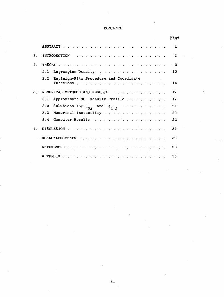
CONTENTS
Page
ABSTRACT . . . . . . . . . . . . . . . . . . . . ... 1
1. INTRODUCTION . . . . . . . . . . . . . . . . . . . . 2
2. THEORY . . . . . . . . . . . . . . . . . . . . . ... . . 6
2.1 Lagrangian Density . .. .... .. ... .. . 10
2.2 Rayleigh-Ritz Procedure and Coordinate
Functions .. .......... . ... . . . . 14
3. NUMERICAL METHODS AND RESULTS . ........... 17
3.1 Approximate DC Density Profile . .... .... 17
3.2 Solutions for CSj and ,j . . . . . . . . . . 21
3.3 Numerical Instability . ............. 22
3.4 Computer Results . ..... . . ......... 24
4. DISCUSSION . ..... .. . .... . .... . . ... . 31
ACKNOWLEDGMENTS .................... 32
REFERENCES .................. ..... 33
APPENDIX . . . . . . . . . . . . . . . . . . . . ... 35
ii

FIGURES
Figure Page
1 Definition of plasma perturbation . ... . . . 8
2 Plasma column geometry . ........ .... . . 13
3 Comparison between (22) (indicated by dots),
and Parker's density profile,for the
parameters given in Table 1 . ........... 18
24 Approximate solutions for 1/A = 72, = 1 . . . . . 26
5 Approximate solutions for 1/A = 510, 1 .... 27
6 Approximate solutions for 1/A = 4500,C =1 . . . 28
7 Dipole resonance spectrum of Tube No. 1
(Parker et al.), compared with estimates
by the variational method (indicated by
crosses). The value 7 = 3 has been used. . . 29
iii

TABLES
No, Page
Parameters used in (22), and Figure 3, for a
mercury-vapor positive column. The conversion
between l/A 2 and l/AD is obtained by the
calculation of Parker (1963) ............ 19
2 Dipole resonance frequency estimates obtained
with Ar = 0.05. Significant numerical
instability sets in when N 8 . The 'best
estimates' are obtained with Ar = 0.01
and N = 9 ....... . . . ............... . . . . . 23
iv
VARIATIONAL CALCULATIONS FOR RESONANCE OSCILLATIONS
OF INHOMOGENEOUS PLASMAS
by
Y-K. M. Peng and F. W. Crawford
Institute for Plasma Research
Stanford University
Stanford, California 94305
ABSTRACT
In this paper, the electrostatic resonance properties of an inhomo-
geneous plasma column are treated by application of the Rayleigh-Ritz
method. In contrast to Parker, Nickel, and Gould (1964), who carried
out an exact computation, We have used a description of the rf equation
of motion and pressure term that allows us to express the system of
equations in Euler-Lagrange form. The Rayleigh-Ritz procedure is then
applied to the corresponding Lagrangian to obtain approximate resonance
frequencies and eigenfunctions. An appropriate set of trial coordinate
functions is defined, which leads to frequency and eigenfunction esti-
mates in excellent agreement with the work of Parker, et al. (1964).
1. INTRODUCTION
This paper is concerned with the use of the Rayleigh-Ritz procedure
to estimate the electron resonance frequencies of a warm inhomogeneous
plasma column. This procedure has been extensively applied to single self-
adjoint equations with great success (Mikhlin, 1964). For a system of
equations, however, theoretical extensions have been noted only for the
case of elliptic equations (Mikhlin, 1965). For the equations to be
used here, which are not elliptic, it will be shown that accurate resonance
frequencies can be predicted,provided that a certain set of coordinate
functions is defined.
Previous theoretical treatments of the electron resonance problem
give predictions which agree well with experimental data. However, these
approaches have encountered difficulties stemming from the inhomogeneous
electron density profile. For example, Parker, Nickel, and Gould (1964)
solved numerically an appropriate fourth-order differential equation for
the rf potential in a cylindrical positive column. Because of the exponential
nature of the solutions in the cutoff region, their calculations were
limited by the condition, a / D < 4500, where a is the column
radius, D (= E0 KT/ne2 ) is the mean-squared Debye length, and nO
is the mean electron density in the column. Baldwin (1969) used a
kinetic model in the low-temperature approximation to obtain the external
admittance of a cylindrical plasma capacitor. The appropriate differential
equation was solved after using inner-outer expansions connected through
the resonance region. A WKB description was used for the inner region,
where resonant waves are essentially evanescent, while a travelling wave
description was used for the outer region, where Landau damping is important.
Because the wave nature of the solutions was assumed in the outer region,
2
this theory is appropriate only for higher order resonances. Similar
difficulties have been shown to occur in the simpler one-dimensional model
(Harker, Kino, and Eitelbach, 1968; Miura and Barston, 1971; Peratt and
Kuehl, 1972).
Variational methods offer an attractive alternative to these treatments.
They have been used previously to estimate plasma resonance frequencies
with simplified trial functions. Resonances of a cold inhomogeneous plasma
were treated by Crawford and Kino (1963). Using the variational principle
established by Sturrock (1958), Barston (1963) approximated the dispersion
relations for wave propagation along an infinite cold plasma slab, and
along the interface between two semi-infinite, counter-streaming cold
plasmas. Some general features of the guided waves on a cold, transversely
inhomogeneous plasma column in an axial magnetic field were studied by
Briggs and Paik (1968). These papers (Crawford and Kino, 1963; Barston,
1963; Briggs and Paik, 1968) show that, with appropriate variational
principles and judicious choices of trial functions, useful results can
be obtained with relative ease by the variational approach.
A theoretical variational formulation for the electrostatic resonance
oscillations of a warm, inhomogeneous plasma column in a dc electric or
magnetic field of arbitrary direction was presented by Barston (1965)
with the adiabatic index, 7 , taken as unity. The variational prin-
ciple to be presented here, however, is not restricted in the values of
7 . One important feature in Barston's (1965) analysis is that the
rf electric potential was treated as the solution of the rf Poisson
equation, with the rf electron density considered given. It will be
seen that the coordinate functions to be used here are defined in a
similar fashion. A variational method of the Rayleigh-Ritz type has
3
been applied successfully by Dorman (1969) to a one-dimensional, warm,
and field-free plasma with arbitrary dc density profile. A single
second order differential equation for the electric field was obtained,
and shown to have hermitian operators. The variational principle to
be used here differs from Dorman's (1969) in that we are dealing
directly with a system of Euler-Lagrange equations. In so doing, we
can keep down the order of the equations, and are able to consider
warm inhomogeneous plasmas in more than one dimension.
In this paper, we shall show that by appropriate definitions of the
rf equation of motion and pressure term, the equations of the hydrodynamic
model used by Parker, et al. (1964) become Euler-Lagrange equations. This
will enable us to demonstrate the effectiveness of the Rayleigh-Ritz
procedure in estimating the resonance frequencies of an inhomogeneous plasma.
The associated numerical method mainly involves evaluations of definite
integrals and solutions of finite algebraic eigenvalue equations, and is
applicable over the entireorange of a /XD >> 1 for estimating the first
few resonance frequencies.
In most of the papers that deal with the electrostatic resonance
problem (Crawford and Kino, 1963; Parker et al., 1964; Harker et al., 1968;
Baldwin, 1969; Dorman, 1969; Miura and Barston, 1971; Peratt and Kuehl,
1972), it is assumed that the rf plasma current normal to the glass wall
2 2is zero. However, in the low temperature limit, a / D , the main
resonance frequency seems to agree with that of cold plasma theory,in which
the normal rf plasma current is retained. We consider this problem and
show that the resulting difference in predicted resonance frequencies is
negligibly small for low pressure positive columns.
4
In §2, we present the basic equations, the corresponding Lagrangian,
and the procedure to be applied in the variational approach. In 83, the
numerical methods are explained before comparing computations with those
of Parker et al. (1964). The paper concludes with a brief discussion
in §4.
5

2. THEORY
For a low pressure positive column, moment equations with scalar
pressure and negligible heat conduction are appropriate when the wave
phase velocity is much larger than the thermal speed. For the first few
electrostatic resonances, the wave phase velocity may be scaled to pa ,
where W p[=(e2nO(0)/me0 ) 1/2 is the axial plasma frequency. Thus we require
a/XD > i. A stationary ion background will be assumed, since we are
interested only in electron resonances. Dissipation due to collisions,
and Landau damping, will be neglected. Our analysis will consequently be
valid only for the first few resonances. Also, the analysis will be quasi-
static. Apart from some differences in definition of the rf equation
of motion and pressure term, the equations we shall use are essentially
those used by Parker, et al. (1964). The equations are generalized here
to include dc magnetic field, B and electron drift velocity, v
We have,
an-- + (nv) = 0 , 8-E + e(n-n )= 0
mn -+ v*"v + VP + en (E + v X B) = 0 at + (1)
Specialized to small perturbations, these reduce to the de equations,
O*(nOv O ) = 0 , e 7.E + e (n 0-n ) = 0
(2)mnov ov +VPo+ eno(E + O) = 0 (at r O ,
and rf equations,
an1-t + r'(n vl + nl 0) = 0 , E r£ + en -= ,t 0 -1 *
mn 0 k + ('[)uP 0 + VP1 + '(PP O
+ en0 ( V + E1 + jX B + X Bl ) = (3)
6
where = dg/dt = 2/dt + v.* . In these equations, m and -e are
the electron mass and charge; n and P are the electron density and
pressure; E is the electric field; n I is the ion density; E0 is the
vacuum permittivity; and I is the perturbation displacement for the
electrons (Figure 1).
The magnitude of v0 is relatively small in the plasma region, but
increases in the sheath region from the ion-acoustic speed to roughly the
electron thermal speed at the glass wall (Self, 1963; Parker, 1963). We
shall consequently neglect it in our analysis. However, due to the presence
of non-zero v,' , and an rf electric field at the wall, a non-zero rf
normal current term arises, and hence an rf surface charge term. The
inclusion of this surface charge term, in the cases where the electron
rf excursion exceeds the Debye length, is equivalent to the use of the
dielectric model for a cold plasma column (Crawford, 1965). Further
discussion of this surface charge term will be given in V3.4. With v0
neglected, the following relations become appropriate
no(r) = nO(0)f(r) , f(r) = exp[-ecpO(r)/KTe]
(4)
n= -v(n) , 1 ,
where K is the Boltzmann constant, ~O(r) is the dc column potential,
E (r) = -Vc (r) , (5)
and the first equation of (3) has been used to obtain nl. The rf
electron pressure, P1 , is determined by the adiabatic equation of state,
P(r 0+)/P (r) = n(r-+O)Y/n O (r ) P = n KTe (6)
The form of (6) can be understood by reference to Figure 1, and
follows from the fact that when a cell is displaced from r to r +
7
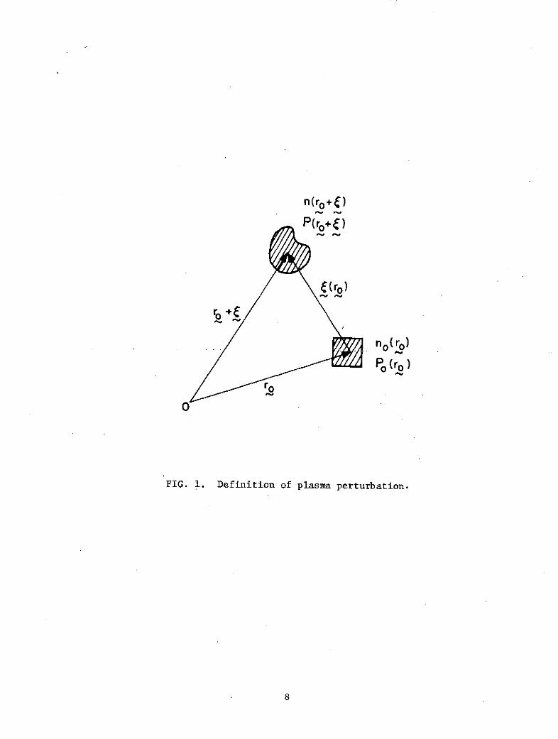
n(ro +)
P(ro+C)
Po (ro)
0
FIG. 1. Definition of plasma perturbation.
8
P is defined for the given cell,rather than for the given position, r-0*
The adiabatic equation of state must consequently be applied to the same
cell, before and after the displacement. Using the usual definition of
perturbations,
P(r) = P (r) + P (r) , n(r) = n0(r) + nl(r) , (7)
and (4), we obtain
P1 = -YPoV' - VP0 . (8)
The rf force law in (3) is obtained by comparing the force laws in (1)
and (2) in the same fashion (Newcomb, 1962).
It is now straightforward to use (4), (5), and (8) to rewrite (3)
in terms of only J and the rf potential, cpl(-P 1 = E
mnC - (7-1)vP 0 .- - 'VP 0 - 0 )
- en 0 ( 1 + -VVP0O - x) = 0 ,
2EV 2 1 + eV.(n0 ) = 0 . (9)
Equations in (9) can be Fourier-transformed, normalized, and expressed
in a cylindrical coordinate system, (r,8), for a column of cylindrical
symmetry,
02f r c 2[ i i
+ D f( r + r R ) + f0r ) = O , (10)
2 c2f, 1 2 ( , 1
0 f C QcO + D r D R r R -r - R e
+ f + , (11)
9
S(R 1 + (Rf R = 0 , (12)
where the derivative with respect to R is denoted by (') and
S0(0) = O , =-r r + (ie )
1(R,O,T) =E dQ1 (R)exp i(CT+L9) , (13)
with i denoting unit vectors. The normalized quantities are defined as
R = r/a , T = Wt , O = W/w ,
Oc = eBO/Bp a ,
2 2 2 2 2 2AD =D/ = T0 e/nO(0)e a = pc/n(0)ea2 , (14)
and a static axial magnetic field, BO , has been included.
2.1 Lagrangian Density
The forms of the force law in (3),and the rf pressure in (7)
represent the important differences from the paper by Parker, et al. (1964)
in that they make (9),as well as (10)-(12),systems of Euler-Lagrange
equations without having to restrict the values of 7 (Barston, 1965).
In one of the models used by Dorman (1969), an appropriate pressure term
similar to (7) was used without the benefit of the rf force law in (3).
As a result, he was able to establish the variational principle only for
the one-dimensional case.
The Lagrangian corresponding to (10)-(12) can be shown to be the
following, by straightforward application of Hamilton's variational principle,
10

12 = fo d(
2 ( l ) t( ,) = D2 A - c2 DB + H
1 1
A fRdR (IrI2 + I2) ' B = fRdR (r + *rO)
O O
H =-A D (T+T) - VOS - I+F+F' < 0
1
T = fRdR''+ 1 21 f r + -r ) + c.e '7- ,2 + . JR=
S z rr r 0 JR=1
1
T' = fRdR r( -) + C*) + C.C.
0
+ 2 [fC*(- r + f r) + ) + c.c.]R=1 '
1
S = fRdR (¢oCr2 + r oC,12)
0
1 1
I fRdR 1 + C + c.c., F = RdR + 12 112)
0 0 R
Rb R
F' = egRdR (l2 IjI2 + RdR (,2 20 R R R
Rb
bRb =Rc (15)
11
where c.c. denotes complex conjugate. Equation (15) is appropriate
to the configuration shown in Figure 2 of a concentric metal cylinder
surrounding a glass tube, of relative permittivity E , that contains
the plasma column. In the expressions for T and T' , the boundary
terms are included to modify the natural boundary conditions on C7
and C. (see for example, Courant and Hilbert, 1953) that would other-
with be unphysical. In the expressions for H and S , 0 0 (r) and VO
are defined as
00(r) = - (r)/VO , VO =- (a)
Substitution of the exact solutions of (10)-(12) would make £2( ,)
zero. We see from (15) that, for negligible ic ' D , and V0 , the
resonance frequencies are determined essentially by the values of I, F,
and F' . Since V0 is approximately proportional to AD (Self, 1963;
Parker, 1963), the effect of higher electron temperature is to raise each
resonance frequency. When Oc 0 , the roots of £2( ,4) = O are
1,2 = QcB/2A [(Q cB/2A) 2 - H/A]1/2 (16)
Since Q and - L are indistinguishable in experimental observations, we
.see that all the resonance frequencies are predicted by (16) to split
in two,in agreement with the theoretical results of Barston (1965), and
Vandenplas and Messiaen (1965). For sufficiently small Oc , when the
values of B and A are not greatly affected by the presence of an
axial static magnetic field, the amount of-the split, IncB/AI , will
be proportional to Oc. This is in agreement with the observed splitting
character of the main dipole resonance frequencies (Crawford, Kino, and
Cannara, 1963; Messiaen and Vandenplas, 1962). Furthermore, since
A IBI, where the equal sign applies when y a ( ' this split is predicted
to be always less than or equal to c
12

FIG. 2. Plasma column geometry.
13
2.2 Rayleigh-Ritz Procedure and Coordinate Functions
For a single linear Euler-Lagrangian equation, the Rayleigh-Ritz
procedure is efficient in obtaining an approximate solution,by use of a
weighted summation of a set of judiciously chosen coordinate functions.
These coordinate functions must be linearly independent and complete,
and satisfy the boundary conditions specified by the problem. The
weighting coefficients that appear in the approximated Lagrangian are
varied independently. This results in a system of algebraic equations
that take the place of the original equation. Theoretically, better
approximations can be obtained by using more coordinate functions. When
eigenvalues are involved, the approximate eigenvalues always converge to
the exact values from above (see for example, Mikhlin, 1964).
Much less attention has been given to the analogous problem for a
system of linear Euler-Lagrangian equations, e.g. (10)-(12), though the
theoretical extension of the variational method to a system of second order
elliptic equations has been mentioned by Mikhlin (1965): the way to set
up the corresponding coordinate functions is similar to that for the single
equation case, i.e. the coefficients of each dependent variable are varied
independently.
For our problem, in which (10)- (12) are not in elliptic form, the
coordinate functions and the coefficients must be more restricted. In the
Appendix to the paper it is shown that acceptable estimates of resonance
frequencies and eigenfunctions can be obtained for our problem provided
that the coordinate functions chosen for each dependent variable are
related by (10)-(12).
By expanding Cr, , and 1 in power series of R, and substituting
in (10)-(12), we see that for small R , r C R - 1 , and W
14
Thus, for ( 1 , the solutions are well behaved at R = 0 . If we
also choose even functions for f(R) and 0 (R) , then 5r and C' are
even in R , and 1 is odd in R , when t is odd, and vice versa.
Since there are no other singularities in (10)-(12), polynomials in R
constitute appropriate coordinate functions for our problem. For convenience,
the coordinate functions chosen for Sr will be
r = R - l - R+2j-1 (j = 1,2,...) , (17)
which conform to the usual assumption of zero normal rf current, since
rj (1) = 0
Rather than choosing C.j and l,j independently, we must determine
them via the original differential equations and (17). After eliminating
1 in (10) and (11), it follows by using the second equation of (4) that
RO2(RC' + - tcr ) = [R Oc Q + t(7-1)A0 ](Rr + '- )e) (18)
With a given expression for o0 (r) , and an assigned value of 0 , e.g.
= 1 , .j can then be easily determined for any given rrj
An immediate question arises concerning the dependence of the resulting
variational estimate of resonance frequencies on the size of 0 chosen
arbitrarily here. We have found that the first few resonance frequencies
-4do not change by more than 10 4 when 0 in (18) changes from 0.4 to 1
for all the values of l/A2 used in this paper. If this were not the
case, an iterative procedure would have to be used, i.e. the resulting
variational estimate of Q would have to be used in (18) to obtain a
new set of j . These would be used in turn to obtain improved frequency
estimates, and so on.
The corresponding coordinate function, lj ' is obtained by solving
(12) (Barston, 1965),with conditions of continuity of potential and normal
displacement across the boundaries defined in Figure 2. According to the
15

discussion given in the Appendix, identical coefficients are assigned to
each set of coordinate functions,
N N N
Cr = aj rj r 6 = aj , 1= a 1 ,j , (19)
j=l j=1 j=1
before substitution in the Lagrangian, 2(,t), of (15). The resulting
Lagrangian then gives the algebraic Euler-Lagrange equation below,
N 2
(Q2Aji - CO B. + Hji)a = 0 (i 1, 2, ... , N) ,
1
Aij = fRdR(ri rj + oi j) . (20)
where A. , B.. , and H . -are the matrix-elements of the integrals, A,ij 13 13
B, and H, given in (15), respectively, and are obtained by substituting
the coordinate functions in a fashion given by the above A.. expression.
Equation (20) can be transformed into a generalized eigenvalue problem
(Dorman, 1969)
2N
S(2Aij - B. )b. 0 (i = 1,2,... , 2N)
I 'j=l
b. (ai,a ) (j = 1,2,..., 2N, i = 1,2,... , N) ,
-H 0 0 -H
A ( B =(+ ) (21)
with superscript + signifying the transposition of a matrix. Equation (21)
is now solvable by standard computer codes.
16

3. NUMERICAL METHODS AND RESULTS
The computing procedure is straightforward:
(i) read in physical and computational parameters,
(ii) compute coordinate functions j , ., and all other functions
appearing in the Lagrangian, P2( ,i) , at intervals Ar ,
(iii) compute 22 (Q,) by Simpson's rule to obtain Aij , B..ij , and
H.. , and
(iv) solve (21) for Q and aj ,and compute relevant eigenfunctions for
N, N-1, and N-2 coordinate functions.
3.1. Approximate DC Density Profile
A density profile which approximates Parker's results (Parker,
1963), and is convenient for both analytical and numerical manipulation,
is given by
f(R) = exp[- 0 (R)] , 40 (R) = iR 2 + (1-)Rh , (22)
where h(> 2) is an even integer, < 1 , and [= V0/A ] is the wall
value of the potential function, J(r) , used by Self (1963) and Parker
(1963). The particular form of (22) is used to justify the choice of
coordinate functions of (17). Furthermore, with the use of (22), Cej
and l,j can now be solved analytically in terms of power series in R,
in addition to the numerical solutions of (12) and (18). Comparison of
the solutions by the two methods will provide an estimate of the degree
of accuracy achieved in obtaining 0,j and l1,j
The values of P and h are varied until f(r) best approximates,
by least-square deviation, the profile given by Parker for specified values
of AD and ~ . The resulting profiles are shown in Figure 3, and the
corresponding values of p and h are given in Table 1. It will be
seen that as increases in value, (22) decreases in accuracy because
17

f(R) f(R)
(a) (d)
C R
() I (e)
1 0
FIG. 3. Comparison between (22) (indicated by dots), and Parker's
density profile, for the parameters given in Table 1.

Table 1
Parameters used in (22), and Figure 3, for a mercury-vapor
positive column. The conversion between l/A2 and 1A2
D Dis obtained by the calculations of Parker (1963).
2 2 2 21/A 1/AD 1 h E2 t 2R
2 1 * 4a 3.4 X 10 7.2 X 10 6.72 0.447 4 6.2 X 10 - 4
b 1.3 X 10³ 5.1 X 10² 6.60 0.221 8 i.3 X 10-4
c 8.2 X 10³ 4.5 X 10³ 6.52 0.159 20 t6.2 X 10 - 4
d 6.7 X 10⁴ 4.3 X 10⁴ 6.44 0.142 54 t2.9 x 10- 3
e 6.2 X 10⁵ 4.2 X 10⁵ 6.40 0.141 156 t7.5 X 10 - 3
f o m 1.08 0.644 12 tl.3 x 10-4
19

of the increasing degree of steepness displayed by the density profile
in the sheath region. At zero temperature, the sheath is omitted and
an accurate approximation can again be obtained. The approximation of
(22), however, was found to be sufficient to give accurate frequency
and eigenfunction estimates for all of the values of 1/A listed in
Table 1.
20
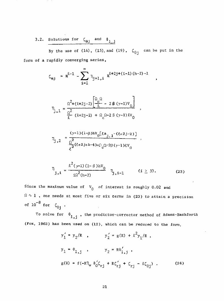
3.2. Solutions for C j and l,j
By the use of (14), (15),and (19), C6j can be put in the
form of a rapidly converging series,
j =R -1 - j+l,i R+2j+(i-l)(h-2)-1
i=l
j 2+(Z+2j-2)- - 28 (7 -l)V0
- (Z+2j-2) + ic -2 B (7 -1)Z£V
(7-1)(i-P)hVO[Jaj, 1-(i+2j-2)]
2(C+ 2 j+ h - 4 )+ c - 2 (7y- 1 ) v O
-2(r-)(i- 4)hV0j,i 2 j ,i-1 (i > 3). (23)iQ 2(h-2)
Since the maximum value of V0 of interest is roughly 0.02 and
Q2 ' 1 , one needs at most five or six terms in (23) to attain a precision
-8of 108 for C@j .
To solve for 01,j , the predictor-corrector method of Adams-Bashforth
(Fox, 1962) has been used on (12), which can be reduced to the form,
S = 2 /R , 2
= g(R) + k2 1 /R
1 l,j ' Y2 = Rl,j '
g(R) = f(-R1w 00rj + R 'j + j - £C j) (24)21rj rj rj
21

Since the complementary solution of (24) is N y R and itsl,j 1
P R +2jparticular solution, yl , is proportional to R near r = 0 ,
P' P/l (0) and y2 (0) are both equal to zero. So the starting values of
P Py and y2 are well-behaved, and easily obtained by Taylor series
expansion near R = . The total solution of 1,j can then be written
as
l, = c R + l , (25)
where cj is determined by imposing the boundary conditions of 1
By making the interval Ar = 0.01, and using double precision, ij-8
can be calculated to within 10 . This is arrived at, first, by com-
paring results that use different values of 6r , and secondly, checking
against solutions of (12) obtained by power-series expansions in R
3.3 Numerical Instability
In the process of solving the algebraic equation,(21), the size
of N is limited by the inaccuracy involved in obtaining A.. , etc.
This inaccuracy introduces a numerical instability whenever the coordinate
functions are not orthogonal functions with respect to the differential
operators of (10)-(12) (Mikhlin, 1971, Chap. 2). The situation is best
illustrated by an example in which the dipole resonance frequencies
corresponding to Figure 3(b) are calculated for different values of N
while holding the size of Ar constant at 0.05.
As shown in Table 2, as N is increased from 2 , the first few
resonance frequencies are approached from above with rapidly stabilized
estimates. When N is increased beyond 8, undesirable fluctuations
larger than 10- 4 , and clearly erratic changes in the values of D , start
to appear. In the case N = 9, for example, one would obtain an erroneous
22

Table 2
Dipole resonance frequency estimates obtained with Ar = 0.05
for the case of Figure 3(b). Significant numerical insta-
bility sets in when N 8 . The 'best estimates' are
obtained with Ar = 0.01 and N = 9
N Main First Second Third Fourth
Best estimates: 0.4447 0.7099 0.8746 0.9924 1.080
2 0.4703 0.8813
3 0.4486 0.7446 0.9250
4 0.4450 0.7155 0.8818 1.022
5 0.4448 0.7119 0.8757 0.9958 1.084
6 0.4448 0.7117 0.8753 0.9956 1.084
7 0.4448 0.7104 0.8751 0.9947 1.082
8 0.4448 0.7098 0.8748 0.9921 1.081
23
fundamental resonance frequency. Characteristic of the variational
nature of the Lagrangian, £2(0,t), more serious errors are found in
the approximate eigenfunctions, than in the resonance frequencies. The
optimal combination of N and Ar , that produces acceptable results
in the shortest computation time, can be obtained by trial and error.
Repeated solution of (21) for a few adjacent values of N thus becomes
an economical technique: this requires computation of the matrices A..
etc. only once, and offers safeguards against obtaining erroneous results
due to numerical instabilities.
3.4 Computer Results
As a practical example, the approximate density profiles given
in Table 1 have been used to predict dipole resonances for Tube No. 1
used by Parker, et al. (1964) (t = 1; a = 0.5 cm; effective relative
permittivity at the surface of the column Keff 1 = 2.1). The
computation time varies roughly as N2 . With N = 10, a typical calcu-
lation takes about 40 seconds, and requires a core space of less than
100K bytes in an IBM 370/67 machine.
The resulting approximate solutions for gri , nl' 1' , and (p
are plotted in Figures 4-6. The density and the radial electric field
solutions, n1(R) and 1 resemble very closely those given by Parker, et al.
(1964), and Parbhakar and Gregory (1971), respectively. The relative
amplitudes of gr and shown in these figures are retained, revealing
that as I/AD increases, Sr progressively dominates over (e. For
1/AD > 4500 , it will be seen that the perturbations should be progressively
compressed toward the sheath region as 1/A increases in value. These
24
solutions are not reproduced here because they also exhibit undesirable
oscillations with wavenumber equal to N , an expected characteristic
when we try to approximate rapidly varying functions with truncated
polynomials. Since only a moderate computer storage is used for N 10 ,
there is room to increase N, and decrease Ar, to obtain better approxi-
mate solutions. However, this is considered unimportant for our purpose,
since we are able to obtain good frequency estimates for this region with
N : 10, as Figure 7 reveals.
The corresponding estimates of resonance frequencies are shown in
Figure 7. Since the electron temperature corresponding to the experimental
resonance data of Parker et al. (1964) was adjusted to fit their theoretical
spectrum, it would be reasonable for us to make a similar adjustment. As
is evident from Figure 7, however, no such adjustment is necessary. Indeed,
our result seems to be in slightly better agreement with the T = 3 eVe
data. The minor differences between the two theoretical results probably
come from the differences in the rf equation of motion and pressure
term used in the two treatments
Similar to other papers (Crawford, 1964; Parker et al. 1964; Harker
et al. 1968; Baldwin, 1969; Dorman, 1969; Miura and Barston, 1971; Peratt
and Kuehl, 1972), we have assumed zero normal rf plasma current density
at the glass wall,through the form of Crj in (17). This is appropriate
when the plasma is sufficiently warm that the electron excursion velocity
is much smaller than the thermal speed,and f(l) << 1 . This assumption,
however, is inconsistent with the dielectric model for a cold plasma
column, where normal rf plasma current must be included. It is of
interest to ask why the main resonance frequency of a warm plasma column,
25
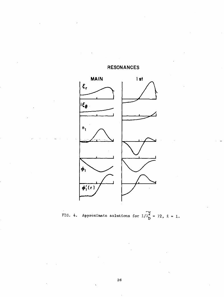
RESONANCES
MAIN I st
n
FIG. 4. Approximate solutions for 1/A = 72, k =
26

RESONANCESMAIN I st 2nd
r
n I,
FIG. 5. Approximate solutions for 1/ = 510, k = 1
27

RESONANCES
MAIN Ist 2 nd
r
FIG. 6. Approximation solution for 1/X = 4500, Z = 1
28

3.01TUBE NO. I- DIPOLE
1 a = 0.5cmKeff= 2 .1
2 .0 + Te= 3eV
0 2 nd
co 0 stI3 o oI.o-. .l +0 .1, + - - ------- + +
0 0 00. 0_' o oo +
oo
IO' I03 104 IOs o
I/A'
FIG. 7. Dipole resonance spectrum of Tube No. 1 (Parker et al.), compared with
estimates by the variational method (indicated by crosses).
in the limit of low temperature, approaches the principal resonance of
a cold plasma column. To answer this question, we need only change (17)
to
Crj = R-1+ (j = 1,2,...), (26)
and impose the requirement of continuity of normal displacement in the
form
(1 ) + f(1)Cr(1) = cg(1 + ) . (27)
The resulting solutions of Cr are found to be only slightly different
from the previous case near R = 1 [Figures 4-6, where the dashed lines
correspond to the use of (17)]. Furthermore, the main resonance is
lowered by less than 1 per cent for all of the values of 1/ used
here, including the case l/A . This is well within the experi-
mental errors.
30
4. DISCUSSION
In this paper, we have applied the Rayleigh-Ritz procedure to a system
of three Euler-Lagrangian equations that describe the electron resonances
of a nonuniform warm plasma column. It is shown that accurate frequencies
for the first few resonances can be obtained for the entire range of
1/A >> 1 . Results which agree closely with those of Parker, et al.
(1964) have been obtained
Contrary to the case of a system of elliptic equations, where the
coefficients are assigned independently to each dependent variable
(Mikhlin, 1971), we have found that for (10)-(12), the same coefficient
must be assigned to each set of coordinate functions, e.g. (19). In
addition to the usual requirements,that the coordinate functions must be
linearly independent and complete, we have chosen that they be set up in
accordance with (10)-(12).
The present method can be easily modified to include the effects
of electron dc drift, dc magnetic field, and ion motion. With the axial
dimensions and rf magnetic field included, this procedure would be efficient
in solving travelling wave problems in a nonuniform plasma waveguide.
31
ACKNOWLEDGMENTS
The authors are indebted to Drs. K. J. Harker and H. Kim for many
useful discussions. The work was supported by the National Aeronautics
and Space Administration.
32

REFERENCES
Baldwin, D. E. 1969, Phys. Fluids, 12, 279.
Barston, E. M. 1963, Phys. Fluids, 6, 828.
Barston, E. M. 1965, Phys. Rev., 139, A394.
Briggs, R. J. and Paik, S. F. 1968, Int. J. Electron., 23, 163.
Courant, R. and Hilbert, D. 1953, Methods of Mathematical Physics, Vol. 1,
Interscience, p. 208.
Crawford, F. W., Kino, G. S. 1963, C. R. Hebd. Seanc. Acad. Sci.,
Paris, 256, 1939 and 2798.
Crawford, F. W., Kino, G. S. and Cannara, A. B. 1963, J. Appl. Phys.,34,
3168.
Crawford, F. W. 1964, J. Appl. Phys., 35, 1365.
Crawford, F. W. 1965, Int. J. Electron., 19, 217.
Dorman, G. 1969, J. Plasma Phys., 3, 387.
Fox, L. 1962, Numerical Solution of Ordinary and Partial Differential
Equations, Addison-Wesley, p. 29.
Harker, K. J., Kino, G. S., and Eitelbach, D. L. 1968, Phys. Fluids, 11,
425.
Messiaen, A. M. and Vandenplas, P. E. 1962, Physica, 28, 537.
Mikhlin, S. G. .1964, Variational Methods in Mathematical Physics, Pergamon.
Mikhlin, S. G. 1965, The Problem of the Minimum of a Quadratic Functional,
Holden-Day, p. 148.
Mikhlin, S. G. 1971, The Numerical Performance of the Variational Method,
Wolters-Noordhoff.
Miura, R. M. and Barston, E. M. 1971, J. Plasma Phys., 6, 271.
Newcomb, W. A. 1962, Nucl. Fusion, Supplement, Part 2, 451.
Parbhakar, K. J. and Gregory, B. C. 1971, Can. J. Phys., 49, 2578.
33
Parker, J. V. 1963, Phys. Fluids, 6, 1657.
Peratt, A. L., Kuehl, H. H. 1972, Phys. Fluids,15, 1117.
Parker, J. V., Nickel, J. C., and Gould, R. W. 1964, Phys. Fluids, 7,
1489.
Self, S. A. 1963, Phys. Fluids, 6, 1762.
Sturrock, P. A. 1958, Ann. Phys., 4, 306.
Vandenplas, P. E. and Messiaen, A. M. 1965, Nucl. Fusion, 5, 47.
34

APPENDIX
Here we shall show that the coordinate functions, crj I ,ej ' and
,j, must be assigned the same coefficients, aj , for the Rayleigh-
Ritz procedure applied to £2(cA) of (15) to be successful: it will
be shown that, by restricting these coordinate functions according to
(10)-(12), the appropriate Rayleigh-Ritz procedure can be established.
A system of second order elliptic equations can be written as
(DjkU)' + XEjkU = 0 , Djk = D kj , Ejk = Ekj (A.1)
thwhere Uk is the k dependent variable, the matrices Djk and Ejk
are functions of the independent variable x , the eigenvalue is X( 0),
and the summation convention has been used. Ellipticity demands that
Djkja k > 0 , Ejkj Ck ~ 0, (A.2)
for any real non-zero vector a. . The solutions of (A.1) then admit
of variational estimates, as outlined by Mikhlin (1965).
When we apply the Rayleigh-Ritz procedure to the Lagrangian for (A.1),
1
L = dx (DjkUjUk - X EjkUjUk) , (A.3)
0
the coefficients preceding the coordinate function for each Uk can be
varied independently. Suppose a set of legitimate trial functions,
Uk = CkVk (summation convention not used here) with coefficient Ck , are
used in (A.3). Because of (A.2),we can obtain crude estimates of
larger than the lowest eigenvalue,even if only one of the Ck is non-zero.
If the same procedure is applied to the Lagrangian in (15), we will
obtain erroneous estimates of L1 . Consider the case of a cold, uniform
plasma column with B0 = 0 , so that H =-I + F + F' . Suppose C
35 r
35
C and C are the coefficients for the coordinate functions rj
CrO and ij , respectively. Then if C = , the value of the R
estimate will be zero, and fail the requirement of the Rayleigh-Ritz
sequence.
Consequently, to make (-H/A)1/2 from (15) at least non-zero, we
must use a single coefficient for each set of the coordinate functions
Crj ' j , and 1,j Merely making Cr = CO = C a. is insuffi-
cient to produce a legitimate Rayleigh-Ritz sequence, because the value
of i for example, can be arbitrarily small in comparison with
Crj and Cej , making the Q estimates also arbitrarily small. We
see that restricting these coordinate functions according to (10)-(12),
is sufficient to reduce the resulting approximated Lagrangian to a single
Euler-Lagrange equation. The appropriateness of the resulting Rayleigh-
Ritz procedure can then be guaranteed. It is conceivable, of course,
that there may be less restrictive choices of appropriate coordinate
functions corresponding to the Lagrangian in (15), but we have not chosen
to pursue this point.
36