Going from microscopic to macroscopic on non-uniform...

Going from microscopic to macroscopic on non-uniform

growing domains

Christian A. Yates,1, ∗ Ruth E. Baker,2, † Radek Erban,3, ‡ and Philip K. Maini4, §

1Centre for Mathematical Biology,

Mathematical Institute, University of Oxford,

24-29 St Giles’,Oxford OX1 3LB, UK



24-29 St Giles’, Oxford OX1 3LB, UK

3Centre for Mathematical Biology and Oxford

Centre for Collaborative Applied Mathematics,


24-29 St Giles’, Oxford OX1 3LB, UK



24–29 St Giles’, Oxford OX1 3LB, UK

(Dated: July 10, 2012)

1

Abstract

Throughout development, chemical cues are employed to guide the functional specifi-

cation of underlying tissues while the spatio-temporal distributions of such chemicals are

often influenced by the growth of the tissue itself. These chemicals, termed morphogens,

are often modeled using partial differential equations (PDEs). The connection between

discrete stochastic and deterministic continuum models of particle migration on grow-

ing domains was elucidated for the first time in (R.E. Baker, C.A. Yates and R. Erban.

From microscopic to macroscopic descriptions of cell migration on growing domains. Bull.

Math. Biol., 72(3):719-762, 2010) in which the migration of individual particles was mod-

eled as an on-lattice position-jump process. We build on this work by incorporating a

more physically reasonable method of domain growth. Instead of allowing underlying lat-

tice elements to instantaneously double in size and divide, we allow incremental element

growth and splitting upon reaching a pre-defined threshold size. Such a method of domain

growth necessitates a non-uniform partition of the domain. We first demonstrate that an

individual-based stochastic model for particle diffusion on such a non-uniform domain par-

tition is equivalent to a PDE model of the same phenomenon on a non-growing domain,

providing the transition rates (which we derive) are chosen correctly and that we partition

the domain in the correct manner. We extend this analysis to the case where the domain

is allowed to change in size, altering the transition rates as necessary. Through a novel

application of the master equation we derive a PDE for particle density on this growing

domain and corroborate our findings with numerical simulations.

PACS numbers: 87.10.Mn, 87.15.nr, 87.17.Pq, 87.17.Aa, 05.40.-a, 87.15.Ya

∗[email protected]; http://people.maths.ox.ac.uk/yatesc/†[email protected]; http://people.maths.ox.ac.uk/baker/‡[email protected]; http://people.maths.ox.ac.uk/erban§[email protected]; http://people.maths.ox.ac.uk/maini

2

I. INTRODUCTION

When modeling particle diffusion we often have a choice between macroscopic

population-based models and micro/mesoscopic individual-based models. The latter

are often formulated as a population of individuals undergoing an on-lattice random

walk [1–3]. Considering multiple short bursts of experimental data it may be possible

to derive the coefficients of a microscopic Fokker-Planck equation or, equivalently, a

stochastic differential equation, which describes the movement rules for individual

particles, using the so-called ‘equation-free technique’ [4, 5]. This approach has

been successful for the modeling of biological motion on larger scales, specifically for

locust movement [6, 7]. It may also be possible to derive the transition rates for a

mesoscopic position-jump model by simply overlaying a grid on experimental data.

However, these micro/mesoscopic models are generally mathematically intractable

and, when considering large numbers of individuals, will take (in general) orders

of magnitude longer to simulate than macroscopic population-based models. Addi-

tionally, macroscopic models are often more straightforward to write down and are

easier and faster to simulate, especially for large particle numbers. Partial differen-

tial equation (PDE) models are also amenable to mathematical analysis via a range

of well characterized techniques.

We first present a macroscopic approach in which a characteristic of the whole

population is considered directly. This approach leads to a PDE model where the

diffusion of particles can be modeled by analogy to Fick’s law:

∂u

∂t= ∇ · (D∇u) . (1)

The derivation of a macroscopic diffusion coefficient, D, from a microscopic model

is relatively simple for many microscopic models [8], although it can be decidedly

more difficult when particles are modeled as having a finite size rather than being

point particles, as in the case of the cellular Potts model [9, 10]. For some models

the diffusion coefficient, D, depends on the particle density, u [2, 11]. In some cases

it may even be replaced by a more general (anisotropic) diffusion tensor, obtained by

the diffusion approximation of the transport equation that describes the underlying

3

random walk model [12, 13].

A. Incorporating domain growth

Using standard conservation of matter arguments, as in the case of the stationary

domain, in combination with the Reynolds transport theorem, we can alter the

classical diffusion equation (1) to account for a time-dependent growing domain,

Ω(t). We arrive at the following partial differential equation (PDE) for the particle

density, u(x, t):

∂u

∂t+ ∇ · (vu) = ∇ · (D∇u) , (x, t) ∈ Ω(t) × [0, ∞), (2)

where v(x, t) = dx/dt is the velocity field generated by domain growth (see Baker

et al. [14] for a detailed derivation).

In a previous work, Baker et al. [14], we demonstrated an equivalence between a

stochastic individual-based model (a position-jump model on a regular underlying

lattice of elements) incorporating domain growth and a continuum representation

of the form of equation (2). Domain growth was implemented through the instanta-

neous doubling and dividing of underlying lattice elements. We would like to move

away from this unphysical description of growth to a model where the underlying

lattice elements grow and divide in a more natural, continuous way. Stochasticity

will be introduced by making growth of the individual tissue elements a random

process. The consideration of domain elements of differing sizes motivates the con-

sideration of non-uniform domains. We expect that this work will provide us with

a more realistic method of simulating stochastic pattern formation on growing do-

mains. Potential biological application areas include modeling the movement of cells

in response to chemical signals [1] and the simulation of morphogen concentrations

on developing embryos [15] amongst others [16].

B. Outline

As an introduction to the area we will briefly summarize our previous work on

the equivalence between stochastic and continuum models of diffusion in one di-

4

mension both with and without domain growth [14]. In Baker et al. [14] we were

able to incorporate the important two-way feedback between particle density and

domain growth into the equivalence framework. In this paper, however, we will

focus purely on the technical aspects of incorporating non-uniform domain parti-

tions into our equivalence framework and leave the inclusion of the dependence of

domain growth on particle density for a future work. In Section III the desire for a

more physically reasonable description of domain growth will stimulate us to con-

sider stochastic models with non-uniform domain division which we will investigate

initially on a non-growing one-dimensional domain. We also discuss the important

distinction between two different types of domain partition, which were equivalent

on the uniform domain. In Section IV domain growth will be introduced. In Section

V we demonstrate an equivalence between our new model and a PDE describing the

change in particle density across the growing domain by consideration of a master

equation. We corroborate our findings in Section VI with numerical simulations

which demonstrate the equivalence of the two models. In Section VII we conclude

with a short discussion of the limitations and possible consequences of our work.

II. MODELLING PARTICLE MIGRATION IN FIXED DOMAINS

All the individual, particle-based stochastic models outlined in this paper con-

sider some fixed (unless otherwise stated) population of N particles restricted to

move on a finite domain. The domain is not, for the moment, considered to be

biological tissue. Instead we consider a general framework which will allow us to

subsequently incorporate biologically motivated features. Nevertheless we still refer

to an individual section of the domain as a tissue element, interval or box through-

out the rest of this paper. Particles are allowed to move via random diffusion. We

assume, unless explicitly stated, that there are no reactions between particles and

no particle degradation on the time-scale of interest and that particles may not

enter or leave the domain, although such effects could be easily incorporated into

our framework and have been in other similar frameworks (see Baker et al. [14]).

These zero flux boundary conditions in combination with the absence of particle

5

creation/degradation render the population constant in time. The first model pre-

sented for this process is at a discrete particle-level in which all the particles are

modeled as identical individuals moving subject to probabilistic rules.

Consider the nondimensionalized stationary (time-independent) domain x ∈ [0, 1]

discretized into k intervals each of length ∆x = 1/k. ∆x will be known as the

‘standard interval length’. The random variable denoting the number of particles

in interval i is Ni and the evolution of particle numbers over the whole domain can

be denoted by the vector N (t) = [N1(t), N2(t), . . . , Nk(t)] (On the uniform grid,

described here, particle density and particle numbers will scale by a constant factor,

the length of a tissue interval, so that we can use the terms almost interchangeably.

However, when we come to consider a non-uniform domain partition the numbers of

particles in each interval must be divided by the length of that interval in order to

calculate the particle density in that part of the domain.) Initially, in this stochastic

position-jump model, we assume that the particles are restricted to move on a spatial

grid between points defined to be at the center of each element, and we denote the

transition rates for a particle to move out of interval i to the left as T −i and to the

right as T +i . These rates may depend on the particle density, N , external signaling

factors, s, and time, t. To complete the formulation of the model we specify initial

and boundary conditions. In order to model the conservation of particles on the

domain we assume T −1 = T +

k = 0. This is analogous to zero flux boundary conditions

in a continuum model. Each interval is initialized to contain a particular number of

particles so that the total number across the domain sums to N .

It is possible to construct a reaction-diffusion master equation (RDME) describing

the evolution of particle density, N . Let Pr(n, s, t) be the joint probability that N =

n at time, t, under deterministic external conditions, s, with n = [n1, n2, . . . , nk]

and s = [s1, s2, . . . , sk] and define the operators J+i : Rk → R

k, for i = 1, . . . , k − 1

and J−i : Rk → R

k, for i = 2, . . . , k, by

J+i : [n1, . . . , ni, . . . , nk] → [n1, . . . , ni−2, ni−1, ni + 1, ni+1 − 1, ni+2 . . . , nk],

J−i : [n1, . . . , ni, . . . , nk] → [n1, . . . , ni−2, ni−1 − 1, ni + 1, ni+1, ni+2 . . . , nk].

By considering all the possible particle movements in a time interval δt, small

enough that the probability of more than one particle movement in δt is O(δt), we

6

can write down the RDME as follows [14]:

∂ Pr(n, t)

∂t=

k−1∑

i=1

T +i

(ni + 1) Pr(J+i n, s, t) − ni Pr(n, s, t)

+k∑

i=2

T −i

(ni + 1) Pr(J−i n, s, t) − ni Pr(n, s, t)

. (3)

Consider the vector of stochastic means, defined as

M(t) = [M1(t), . . . , Mk(t)] =∑

nn Pr(n, s, t) ≡

∞∑

n1=0

∞∑

n2=0

. . .∞∑

nk=0

n Pr(n, s, t).(4)

It can be demonstrated that these means satisfy

dM1

dt= T −

2 M2 − T +1 M1, (5)

dMi

dt= T +

i−1Mi−1 −(

T +i + T −

i

)

Mi + T −i+1Mi+1, for i = 2, . . . , k − 1, (6)

dMk

dt= T +

k−1Mk−1 − T −k Mk, (7)

providing T ±i is independent of particle density [1, 14]. Equation (6) is similar to

the master equation for the positional probability of a random walker on a lattice

as derived by Othmer and Stevens [1] and Painter and Hillen [2].

To draw a rigorous correspondence between equations (5)-(7) and a population-

level description of the variation of particle density with time, terms of the form

Mi±1 = M(xi ± ∆x, t) are expanded about xi. Taking transition rates T ±i = d for

i = 1, . . . , k, for example, gives

∂M

∂t(xi, t) = d(∆x)2 ∂2M

∂x2(xi, t) + O((∆x)2), (8)

where M(xi, t) = Mi. Here ∆x = 1/k, the distance between the centers of the

intervals, is the same as the length of each interval. Allowing ∆x → 0 in such a

way[1] that lim∆x→0 d(∆x)2 = D, gives the diffusion equation for particle density,

u(x, t):∂u

∂t= D

∂2u

∂x2, (x, t) ∈ [0, 1] × [0, ∞). (9)

Conservation of particles in the deterministic model can be derived from the moment

equations and correspond to zero flux boundary conditions on u:

∂u

∂x

∣

∣

∣

∣

∣

x=0,1

= 0. (10)

7

III. PARTICLE DIFFUSION ON A NON-UNIFORM DOMAIN

In order to consider a more physically reasonable approach to domain growth than

in previous studies (see [14]), we would like to allow the underlying domain elements

to grow by small increments and then divide upon reaching a critical size, rather than

instantaneously doubling in size and dividing as has previously been implemented

(see Fig. 1). Incorporating incremental stochastic interval growth necessitates the

consideration of domain elements of different sizes. This will affect transition rates

between the elements. For example, if, in a microscopic model, a particle is assumed

to be exhibiting an unbiased, Brownian random walk it will take longer, on average,

for that particle to exit a larger element than a smaller one. To begin with we will

characterize the diffusion process on a non-growing, non-uniform domain, deriving

transition rates for tissue elements of different sizes. Once the correct transition

rates have been established on the stationary domain we will attempt to incorporate

growth into the one-dimensional model.

A. Particle migration on a stationary, non-uniform grid

Now that we are considering a non-uniform grid we must be careful about how

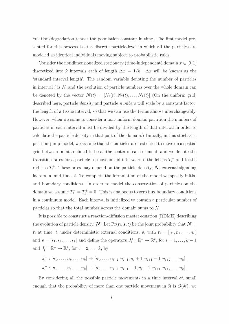
we define our domain partition. There are two natural ways to do this (see Fig. 2).

1. Points x1, x2, . . . , xk are chosen and are associated with intervals, 1, . . . , k,

respectively. The interval edges, y0 = 0, yk = 1 and yi = (xi + xi+1)/2, for i =

1, . . . , k − 1, are then naturally defined in a Voronoi neighborhood sense: a point on

the domain is defined to lie in the interval i if it is nearer to xi than any other xj

for j = 1, . . . , k, j 6= i.

2. The edges of the intervals, y0, y1, . . . , yk, are chosen (with y0 = 1 and yk = 1

defining the end points of the domain) and the point xi associated with interval i,

for i = 1, . . . , k, is defined to be the center of that interval (i.e. xi = (yi−1 + yi)/2

for i = 1, . . . , k).

The Voronoi domain partition is the natural particle-position-focused extension

of the uniform domain partition. The positions where the particles are considered

to lie are defined first and the interval boundaries are defined to bisect these points.

8

(a)

(b)

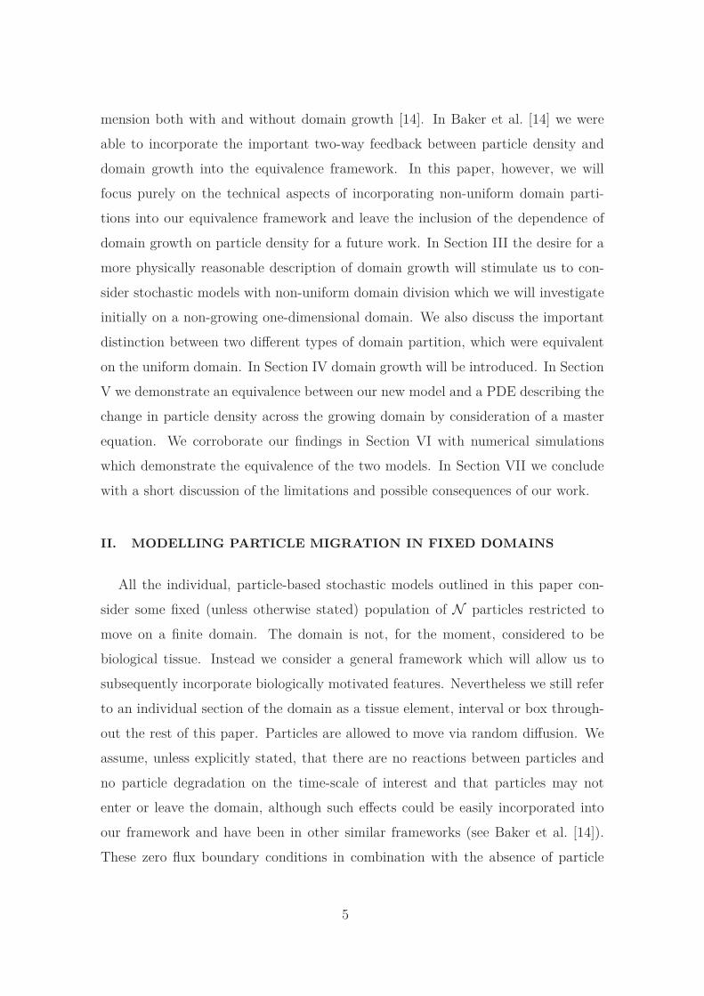
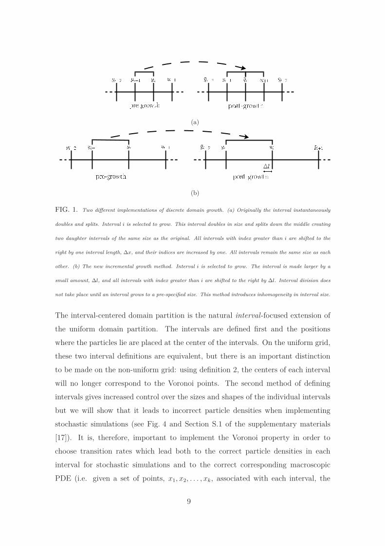
FIG. 1. Two different implementations of discrete domain growth. (a) Originally the interval instantaneously

doubles and splits. Interval i is selected to grow. This interval doubles in size and splits down the middle creating

two daughter intervals of the same size as the original. All intervals with index greater than i are shifted to the

right by one interval length, ∆x, and their indices are increased by one. All intervals remain the same size as each

other. (b) The new incremental growth method. Interval i is selected to grow. The interval is made larger by a

small amount, ∆l, and all intervals with index greater than i are shifted to the right by ∆l. Interval division does

not take place until an interval grows to a pre-specified size. This method introduces inhomogeneity in interval size.

The interval-centered domain partition is the natural interval-focused extension of

the uniform domain partition. The intervals are defined first and the positions

where the particles lie are placed at the center of the intervals. On the uniform grid,

these two interval definitions are equivalent, but there is an important distinction

to be made on the non-uniform grid: using definition 2, the centers of each interval

will no longer correspond to the Voronoi points. The second method of defining

intervals gives increased control over the sizes and shapes of the individual intervals

but we will show that it leads to incorrect particle densities when implementing

stochastic simulations (see Fig. 4 and Section S.1 of the supplementary materials

[17]). It is, therefore, important to implement the Voronoi property in order to

choose transition rates which lead both to the correct particle densities in each

interval for stochastic simulations and to the correct corresponding macroscopic

PDE (i.e. given a set of points, x1, x2, . . . , xk, associated with each interval, the

9

number of particles at xi is independent of how we define the boundaries of the

intervals, since (as we will demonstrate) transition rates are only dependent on

the distances between neighboring points. However, when we come to calculating

particle densities the interval boundaries become important and we can show (see

Section S.1 of the supplementary materials [17]) that the Voronoi domain partition

gives smoothly varying particle densities, which correspond to the derived PDE,

because the interval sizes are related to the transition rates in a unique way.). In

what follows we primarily use the first method to partition our domain into intervals

(known hereafter as Voronoi partitioning). We will, however, give comparisons of

the two partition methods on both fixed and growing domains demonstrating the

propriety of the Voronoi partition. In Section IV C we also discuss when it might

be more appropriate to use the interval-centered domain partition to increase our

control over the interval sizes.

The Voronoi partition implies that the boundaries for interval i will be at yi−1 =

(xi−1 + xi)/2 (left-hand boundary) and yi = (xi + xi+1)/2 (right-hand boundary).

As in the case of the uniform domain, particles are considered to be positioned at

x1, x2, . . . , xk for intervals 1, . . . , k, respectively (see Fig. 2). Intervals 2, . . . , k − 1

will be known as ‘interior’ intervals and intervals 1 and k as ‘end’ intervals.

Previously, the scalings of the transition rates for particles to move between in-

tervals have been specified somewhat artificially by considering equations (5)-(7)

(or their analogues), Taylor expanding the terms at i ± 1 and choosing the scal-

ing so that we return to a macroscopic PDE [1]. Now that we are considering a

non-uniform domain it is not so simple to see what the requisite scaling for each

transition rate should be. In order to ensure correspondence with a PDE the tran-

sition rates should depend in some way on the sizes of the intervals between which

a particle moves. Even if we could guess the transition rates and plug them into

equations (5)-(7) to check that we derive the correct macroscale equation, it would

be preferable to have a microscale justification of these scalings. The transition

rate for a particle at xi should depend on the distance to the associated domain

definition points in the neighboring intervals, xi−1 and xi+1. As such, we consider

a microscale migration process in the interval [xi−1, xi+1]. We will consider this mi-

10

(a)

(b)

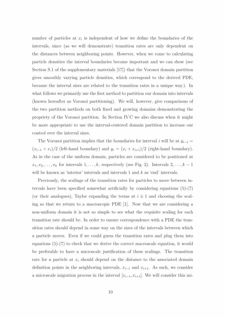
FIG. 2. Two different domain partitions. (a) The Voronoi partition method. Particle positions, xi, are chosen

first and interval i is defined to be all the points which lie closer to xi than any of the other particle positions xj

for j 6= i. This gives interval edges at yi = (xi + xi+1) /2. The Voronoi partition method allows for the natural

incorporation of transition rates which are inversely proportional to interval size, which cannot be done within the

interval-centered framework. (b) The interval-centered definition. Interval boundaries, yi, are defined first and

particles are assumed to lie in the centers of these intervals. In both partitions the distance between neighboring

particle positions, xi and xi−1, is denoted hi = xi − xi−1 and, similarly, hi+1 = xi+1 − xi. For the end intervals

indexed 1 and k, h1 and hk+1 are not defined, so we choose h1 = 2x1 and hk+1 = 2(yk − xk) for consistency with

later results.

croscale process to be simple Brownian motion and expect to derive transition rates

which lead us, via our mesoscale position-jump process, to the diffusion equation

on the macroscale. It is also possible to consider alternative underlying microscale

processes which correspond to biased and/or correlated random walks and which

give rise to advection-diffusion PDEs.

B. From microscopic to mesoscopic

A particle moving according to Brownian motion, with position X(t), obeys a

stochastic differential equation (SDE)

dX(t) =√

2DdWt, (11)

11

where dWt is a standard Wiener process and D is the diffusion coefficient of the

diffusion equation corresponding to this SDE. The probability density function of

the particle, p(x, t), evolves according to the classical diffusion equation:

∂p(x, t)

∂t= D

∂2p(x, t)

∂x2. (12)

Given that we know the initial position of the particle, xi, we have a δ function

initial condition in probability, p(x, t) = δ(x − xi). Finding the transition rates for

the mesoscale position-jump process reduces to a first passage problem. In order to

find the transition rate for moving out of interval i in the position-jump model, we

consider the process in which a particle starting at xi exits the interval [xi−1, xi+1]

and find the probability for it to do so at either end. The interval [xi−1, xi+1] is the

appropriate interval for the calculation of the first passage time since it requires that

the particle finishes its transition in an equivalent position, in an adjacent interval,

to the position at which it started in the original interval. The absorbing boundary

conditions p(xi−1, t) = p(xi+1, t) = 0 complete the formulation of the above problem.

This is a classic first passage problem, the likes of which are dealt with thoroughly

by Redner [18]. Note that the formulation of the first passage problem and hence

the transition rates between intervals are independent of the position of the interval

boundaries. Here we briefly summarize Redner’s derivation of the mean first passage

time.

We first calculate the probabilities for the particle to leave at either end of the

interval, known as the eventual hitting probabilities,

ε−(xi) =xi+1 − xi

xi+1 − xi−1, (13)

ε+(xi) =xi − xi−1

xi+1 − xi−1. (14)

We next calculate the conditional mean exit times to leave the interval at either end,

〈t(xi)〉− =(xi − xi−1)(2xi+1 − xi − xi−1)

6D, (15)

〈t(xi)〉+ =(xi+1 − xi)(xi+1 + xi − 2xi−1)

6D, (16)

which we can use in conjunction with the eventual hitting probabilities (see equations

12

(13) and (14)) to calculate the unconditional mean exit time from the interval,

〈t(xi)〉 = ε−(xi)〈t(xi)〉− + ε+(xi)〈t(xi)〉+,

=1

2D(xi − xi−1)(xi+1 − xi). (17)

We can invert this to give the unconditional mean exit rate and by multiplying

through by the eventual hitting probabilities calculate the conditional mean exit

rates or transition rates,

T −i =

2D

hi(hi + hi+1), (18)

T +i =

2D

hi+1(hi + hi+1), (19)

where, for brevity, as previously defined, we denote hi = xi − xi−1 and similarly

hi+1 = xi+1 − xi. These transition rates are the same as those derived by Engblom

et al. [19] using a finite element discretization of the macroscopic diffusion equation.

Recall the equations relating the mean numbers of particle in each interval (5)-(7):

dM1

dt= T −

2 M2 − T +1 M1,

dMi

dt= T +

i−1Mi−1 −(

T +i + T −

i

)

Mi + T −i+1Mi+1, i = 2, . . . , k − 1,

dMk

dt= T +

k−1Mk−1 − T −k Mk.

Although these equations were derived initially for a uniform mesh, they remain

valid for the non-uniform mesh. We can re-write this equation in terms of particle

densities ui = Mi/li, where li is the length of interval i:

du1

dt=

1

l1

(

T −2 u2l2 − T +

1 u1l1)

, (20)

dui

dt=

1

li

(

T +i−1ui−1li−1 −

(

T +i + T −

i

)

uili + T −i+1ui+1li+1

)

, i = 2, . . . , k − 1, (21)

duk

dt=

1

lk

(

T +k−1uk−1lk−1 − T −

k uklk)

. (22)

We now use Taylor series expansions about position xi on the appropriate terms.

For example,

ui+1 = u(xi+1) = u(xi) + (hi+1)∂u

∂x(xi) +

1

2(hi+1)2 ∂2u

∂x2(xi) + . . . . (23)

13

Allowing the number of domain elements, k, to tend to infinity on the Voronoi

domain partition (i.e. with the appropriate choices of li), implying hi, hi+1 → 0 ∀ i,

we obtain the diffusion equation for particle density, u(x, t):

∂u

∂t= D

∂2u

∂x2, for (x, t) ∈ [0, 1] × [0, ∞), (24)

with the usual zero flux boundary conditions. For a more detailed derivation and a

justification of the necessity of the Voronoi domain partition see Section S.1 of the

supplementary materials [17].

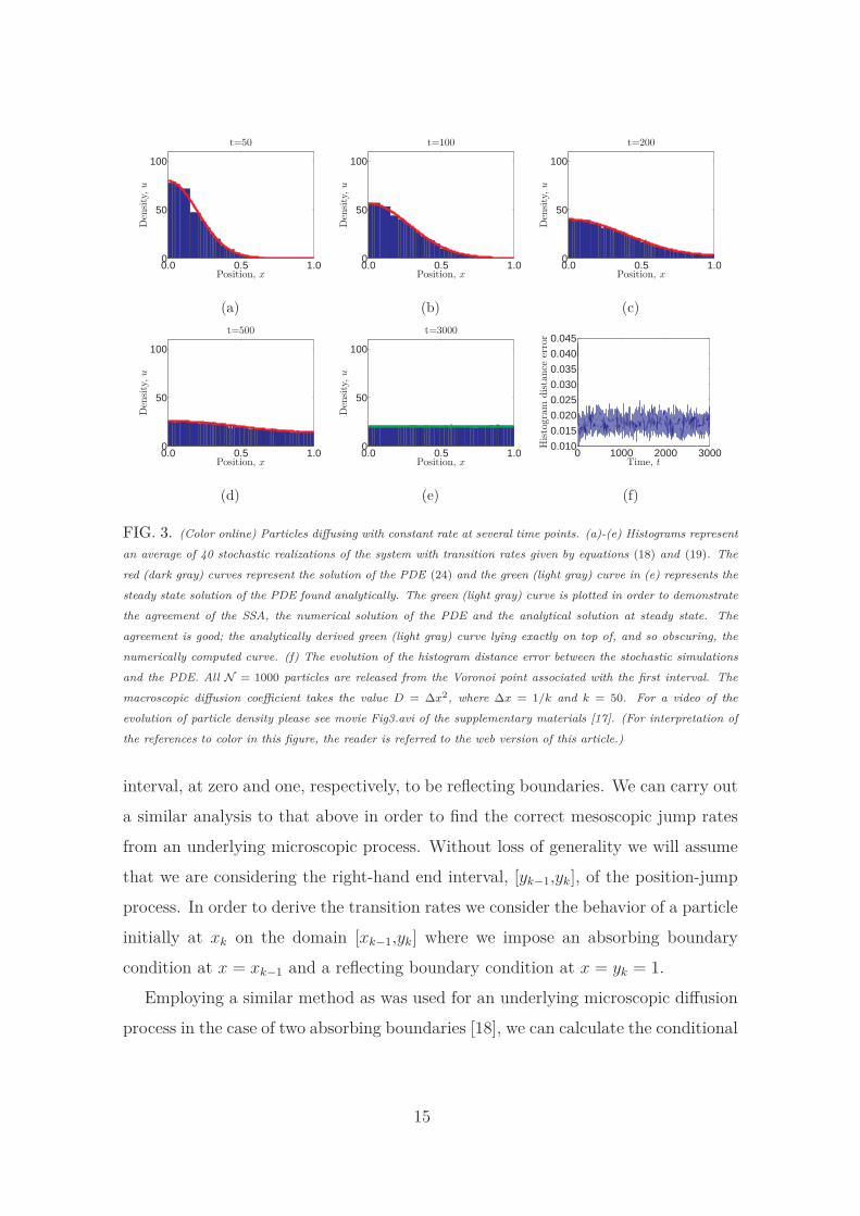
Fig. 3 shows a numerical comparison of the stochastic simulations and the derived

PDE (24). Qualitatively, the PDE for particle density matches the particle density

of the stochastic simulations well. In Fig. 3 (f), in order to give a more quantitative

comparison of the two simulation types, we have plotted the variation of the his-

togram distance error/metric, between the stochastic particle density and the PDE,

over time. The histogram distance metric between two curves (defined at discrete

points), having normalized frequencies ai and bi at point i (i.e.∑

ai =∑

bi = 1), is

given by

D =

∑ |ai − bi|2

, (25)

where the sum is over all i such that either ai 6= 0 or bi 6= 0. Since our particle

densities are defined at non-regular lattice points, xi, we interpolate the value of

the PDE at each lattice point in order to compare the curves. Fig. 3 (f) shows a

low histogram distance error for the duration of the simulation, indicating good

agreement between the two simulation types.

For all simulations we employ Gillespie’s exact Direct Method (DM) Stochastic

Simulation Algorithm (SSA) [20] and release all N = 1000 particle from x1, the

Voronoi point of the first interval.

C. Using a mixed boundary interval to derive transition rates for the end

intervals

In order to implement zero flux boundary conditions on the macroscopic domain

we designate the left-hand end of the first interval and the right-hand end of the last

14

0.0 0.5 1.00

50

100

Position, x

Density,u

t=50

(a)

0.0 0.5 1.00

50

100

Position, x

Density,u

t=100

(b)

0.0 0.5 1.00

50

100

Position, x

Density,u

t=200

(c)

0.0 0.5 1.00

50

100

Position, x

Density,u

t=500

(d)

0.0 0.5 1.00

50

100

Position, x

Density,u

t=3000

(e)

0 1000 2000 30000.010

0.015

0.020

0.025

0.030

0.035

0.040

0.045

Time, t

Histogram

distance

error

(f)

FIG. 3. (Color online) Particles diffusing with constant rate at several time points. (a)-(e) Histograms represent

an average of 40 stochastic realizations of the system with transition rates given by equations (18) and (19). The

red (dark gray) curves represent the solution of the PDE (24) and the green (light gray) curve in (e) represents the

steady state solution of the PDE found analytically. The green (light gray) curve is plotted in order to demonstrate

the agreement of the SSA, the numerical solution of the PDE and the analytical solution at steady state. The

agreement is good; the analytically derived green (light gray) curve lying exactly on top of, and so obscuring, the

numerically computed curve. (f) The evolution of the histogram distance error between the stochastic simulations

and the PDE. All N = 1000 particles are released from the Voronoi point associated with the first interval. The

macroscopic diffusion coefficient takes the value D = ∆x2, where ∆x = 1/k and k = 50. For a video of the

evolution of particle density please see movie Fig3.avi of the supplementary materials [17]. (For interpretation of

the references to color in this figure, the reader is referred to the web version of this article.)

interval, at zero and one, respectively, to be reflecting boundaries. We can carry out

a similar analysis to that above in order to find the correct mesoscopic jump rates

from an underlying microscopic process. Without loss of generality we will assume

that we are considering the right-hand end interval, [yk−1,yk], of the position-jump

process. In order to derive the transition rates we consider the behavior of a particle

initially at xk on the domain [xk−1,yk] where we impose an absorbing boundary

condition at x = xk−1 and a reflecting boundary condition at x = yk = 1.

Employing a similar method as was used for an underlying microscopic diffusion

process in the case of two absorbing boundaries [18], we can calculate the conditional

15

hitting probabilities at x = xk−1 and x = 1 to be

ε−(xk) = 1, ε+(xk) = 0, (26)

which implies we are certain to exit the interval at the left-hand boundary, which

is to be expected. We can calculate the conditional mean exit time at the left-hand

boundary as

〈t(xk)〉− =1

2D(2(yk − xk−1)hk − h2

k). (27)

Rearranging gives the transition rate as

T −k =

2D

hk(2(yk − xk−1) − xk + xk−1),

=2D

hk(hk + hk+1), (28)

recalling the definitions h1 = 2x1 and hk = 2(yk − xk). In an entirely analogous

manner we can derive the transition rate to move right out of the first interval as

T +1 =

2D

h2 (x2 + x1),

=2D

h2 (h1 + h2). (29)

On the uniform domain these transition rates reduce to

T −k = T +

1 =D

h2, (30)

as we might reasonably expect.

D. Comparison with the interval-centered domain partition

In order to demonstrate the propriety of the Voronoi domain partition in compari-

son to the interval-centered domain partition we have carried out similar simulations

to those detailed above with the interval-centered domain partition. The transition

rates are the same as those derived in previous subsections (see equations (18) and

(19) in Section III B and (28) and (29) in Section III C) only now the positions,

xi, where particles are assumed to reside are the centers of the corresponding inter-

vals. It is evident from glancing at Fig. 4 (a)-(e) that the particle densities deviate

16

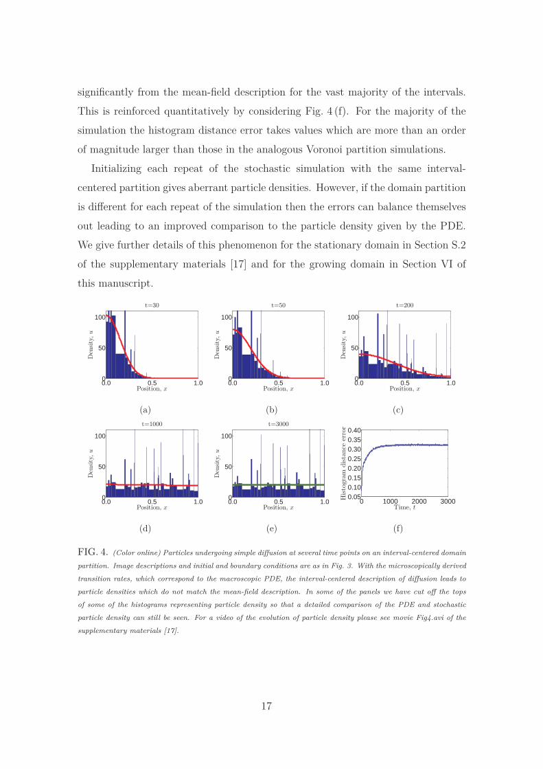
significantly from the mean-field description for the vast majority of the intervals.

This is reinforced quantitatively by considering Fig. 4 (f). For the majority of the

simulation the histogram distance error takes values which are more than an order

of magnitude larger than those in the analogous Voronoi partition simulations.

Initializing each repeat of the stochastic simulation with the same interval-

centered partition gives aberrant particle densities. However, if the domain partition

is different for each repeat of the simulation then the errors can balance themselves

out leading to an improved comparison to the particle density given by the PDE.

We give further details of this phenomenon for the stationary domain in Section S.2

of the supplementary materials [17] and for the growing domain in Section VI of

this manuscript.

0.0 0.5 1.00

50

100

Position, x

Density,u

t=30

(a)

0.0 0.5 1.00

50

100

Position, x

Density,u

t=50

(b)

0.0 0.5 1.00

50

100

Position, x

Density,u

t=200

(c)

0.0 0.5 1.00

50

100

Position, x

Density,u

t=1000

(d)

0.0 0.5 1.00

50

100

Position, x

Density,u

t=3000

(e)

0 1000 2000 30000.050.100.150.200.250.300.350.40

Time, t

Histogram

distance

error

(f)

FIG. 4. (Color online) Particles undergoing simple diffusion at several time points on an interval-centered domain

partition. Image descriptions and initial and boundary conditions are as in Fig. 3. With the microscopically derived

transition rates, which correspond to the macroscopic PDE, the interval-centered description of diffusion leads to

particle densities which do not match the mean-field description. In some of the panels we have cut off the tops

of some of the histograms representing particle density so that a detailed comparison of the PDE and stochastic

particle density can still be seen. For a video of the evolution of particle density please see movie Fig4.avi of the

supplementary materials [17].

17

IV. PARTICLE MIGRATION WITH DOMAIN GROWTH

Previously, growth has been implemented using interval splitting, where an in-

terval doubles in length and divides instantaneously [14]. In order to represent the

growth of the underlying tissue elements more realistically it is preferable to allow

intervals to grow by small increments (more akin to a continual growth process) and

to divide upon reaching a pre-determined size. Several different methods for this

more incremental domain growth description are detailed below.

A. Deterministic domain growth

Each time a particle jumps, we allow each of the intervals to grow an amount

proportional to its length. This produces exponential domain growth of each interval

and hence exponential domain growth of the whole domain. We allow intervals to

grow to roughly (given the stochastic nature of the time stepping) twice the standard

interval size (to 2∆x) before dividing. Upon division, an interval splits into two

equally sized daughter intervals and the particles which resided in that interval are

divided randomly between these two ‘daughter’ intervals using a number drawn

from a binomial random variable, B(ni, 0.5), where ni is the number of particles in

parent interval i (see Baker et al. [14] for a further discussion of possible methods

to reallocate particles into daughter intervals). We call this a “division event”.

Intervals initialized with the same length retain this uniformity and we are not,

therefore, required to consider non-uniform domain partitions. Interval division will

be synchronous and simple to implement.

However, allowing initial inhomogeneity requires the Voronoi partition in order to

produce consistent particle densities (see Section S.1 of the supplementary materials

[17]). Deterministic domain growth maintains the Voronoi property of the domain

and the main issue is how to appropriately repartition the domain once an interval

has become large enough to divide (a “division event”). Ideally we would divide the

parent interval into two equally sized daughter intervals, each half the length of the

original parent interval. Unfortunately, in general, it is not possible to do this whilst

maintaining the Voronoi partition. Instead it is necessary to redefine the boundaries

18

of the two neighboring intervals of the interval that divides (see Fig. 5). We are,

however, at least able to choose daughter intervals that are of equal sizes.

Begin by considering interior intervals. We can express the restriction of main-

taining a Voronoi partition mathematically in terms of the positions of the pre-

division Voronoi point of dividing interval i, xi, those of the two neighboring inter-

vals, xi−1 and xi+1, and the positions of the Voronoi points after division xi−1, xi,

xi+1, xi+2. Where we have relabeled the Voronoi points on the post-division domain

with an ‘over-bar’. In order to ensure that only these three intervals are affected

by the division event we must ensure that the Voronoi points xi−1 and xi+1 remain

unchanged i.e. xi−1 = xi−1 and xi+1 = xi+2. We can express the condition that the

two daughter intervals should be of the same size as

2l = xi+1 − xi−1 = xi+2 − xi, (31)

where l is the length of the daughter intervals. We must also maintain the strict

ordering of the Voronoi points:

xi−1 < xi < xi+1 < xi+2. (32)

These inequalities can be shown (after manipulation) to bound the length of the

daughter intervals above and below:

xi+2 − xi−1

4< l <

xi+2 − xi−1

2. (33)

Choosing the daughter intervals to be half as long as the parent interval, l = (xi+2 −xi−1)/4, would mean choosing the two new Voronoi points to be coincident, xi =

xi+1. At the other extreme, choosing each daughter interval to be the same length

as the parent interval, l = (xi+2 − xi−1)/2, requires each new point to be coincident

with an already existing point, xi = xi−1 and xi+1 = xi+2. Neither of these extreme

situations is acceptable. An unbiased choice, therefore, would be

l =3

8(xi+2 − xi−1) . (34)

This choice fully determines the position of the new Voronoi points (see Fig. 5):

xi =3

4xi−1 +

1

4xi+2, (35)

xi+1 =1

4xi−1 +

3

4xi+2. (36)

19

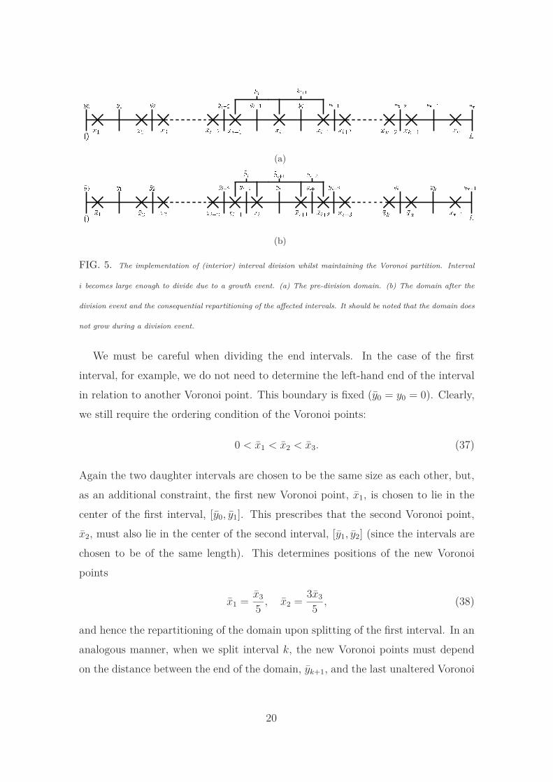
(a)

(b)

FIG. 5. The implementation of (interior) interval division whilst maintaining the Voronoi partition. Interval

i becomes large enough to divide due to a growth event. (a) The pre-division domain. (b) The domain after the

division event and the consequential repartitioning of the affected intervals. It should be noted that the domain does

not grow during a division event.

We must be careful when dividing the end intervals. In the case of the first

interval, for example, we do not need to determine the left-hand end of the interval

in relation to another Voronoi point. This boundary is fixed (y0 = y0 = 0). Clearly,

we still require the ordering condition of the Voronoi points:

0 < x1 < x2 < x3. (37)

Again the two daughter intervals are chosen to be the same size as each other, but,

as an additional constraint, the first new Voronoi point, x1, is chosen to lie in the

center of the first interval, [y0, y1]. This prescribes that the second Voronoi point,

x2, must also lie in the center of the second interval, [y1, y2] (since the intervals are

chosen to be of the same length). This determines positions of the new Voronoi

points

x1 =x3

5, x2 =

3x3

5, (38)

and hence the repartitioning of the domain upon splitting of the first interval. In an

analogous manner, when we split interval k, the new Voronoi points must depend

on the distance between the end of the domain, yk+1, and the last unaltered Voronoi

20

point, xk−1, in the following way:

xk =3xk−1

5+

2yk+1

5, xk+1 =

xk−1

5+

4yk+1

5. (39)

For the purpose of particle redistribution upon splitting we assume that particles

are distributed evenly across each interval. When interval boundaries are redrawn

upon the splitting of interval i the number of particles in the new intervals are chosen

as close as possible (given the integer nature of particle numbers) to

ni−1 =

(

yi−1 − yi−2

yi−1 − yi−2

)

ni−1, (40)

ni =

(

yi−1 − yi−1

yi−1 − yi−2

)

ni−1 +

(

yi − yi−1

yi − yi−1

)

ni, (41)

ni+1 =

(

yi − yi

yi − yi−1

)

ni +

(

yi+1 − yi

yi+1 − yi

)

ni+1, (42)

ni+2 =

(

yi+1 − yi+1

yi+1 − yi

)

ni+1. (43)

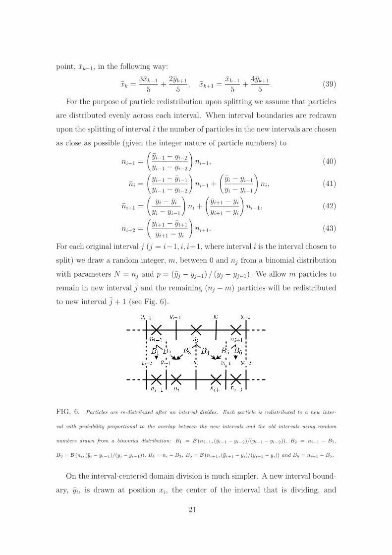
For each original interval j (j = i−1, i, i+1, where interval i is the interval chosen to

split) we draw a random integer, m, between 0 and nj from a binomial distribution

with parameters N = nj and p = (yj − yj−1) / (yj − yj−1). We allow m particles to

remain in new interval j and the remaining (nj − m) particles will be redistributed

to new interval j + 1 (see Fig. 6).

FIG. 6. Particles are re-distributed after an interval divides. Each particle is redistributed to a new inter-

val with probability proportional to the overlap between the new intervals and the old intervals using random

numbers drawn from a binomial distribution: B1 = B (ni−1, (yi−1 − yi−2)/(yi−1 − yi−2)), B2 = ni−1 − B1,

B3 = B (ni, (yi − yi−1)/(yi − yi−1)), B4 = ni − B3, B5 = B (ni+1, (yi+1 − yi)/(yi+1 − yi)) and B6 = ni+1 − B5.

On the interval-centered domain division is much simpler. A new interval bound-

ary, yi, is drawn at position xi, the center of the interval that is dividing, and

21

new interval centers are defined at xi = (yi−1 + xi)/2 = (yi−1 + yi)/2 and xi+1 =

(yi + xi)/2 = (yi + yi+1)/2. All interval centers and edges to the right of the interval

that is dividing are relabeled by increasing their index by one i.e. xj = xj+1 and

yj = yj+1 for j = i + 1, . . . , k. The ni particles that previously resided in interval i

are redistributed evenly into the two daughter intervals.

B. Stochastic domain growth

A possible alternative method for implementing domain growth is to allow inter-

vals to grow in pairs (intervals must grow in pairs in order to preserve the Voronoi

property of the domain. However, when considering the interval-centered domain

partition it is possible, and indeed preferable, to allow intervals to grow individ-

ually) rather than all synchronously as described in Section IV A. We call this a

“growth event”. Growth must be implemented carefully in order to preserve the

Voronoi property of the domain. Intervals i and i + 1 are chosen to grow with a

probability proportional (with constant of proportionality, r) to the size of interval

i: li = (yi − yi−1). All the Voronoi points to the right of xi (xi+1, . . . , xk) move by

a constant amount ∆l to the right, where ∆l is some small fraction of the standard

interval length, ∆x. ∆l is defined such that, when taking the continuum limit, the

ratio ∆l/∆x ≪ 1 remains constant as ∆x → 0 so that terms that are of order ∆l2

may still be neglected in comparison to terms that are of order lj, the length of the

jth interval (see Section V C). The boundary, yi, is then re-drawn ∆l/2 to the right

of its original position. Thus growth causes intervals i and i + 1 to grow by ∆l/2

each (see Fig. 7). The only exception to this rule is for the right-hand-most interval

of the domain where we can simply move the right-hand boundary of the interval

by ∆l without disturbing the Voronoi property. Upon growing to a predetermined

size, ∆xsplit, intervals are divided and particles redistributed in the same manner

as described above. By considering a master equation for the domain length, L(t),

we can show that (see Section S.7 of the supplementary materials [17]), on average,

this process leads to exponential domain growth; L(t) = exp(r∆lt). Crucially this

growth process maintains the Voronoi property of the partition.

22

If we are considering an interval-centered domain partition (which may be justi-

fied in some circumstances, see Sections S.2 and S.8 of the supplementary materials

[17]) we can implement domain growth in a much more straightforward manner.

Growth of interval i occurs with rate proportional to its length, li. Interval edges to

the right of the growing interval (yj for j = i + 1, . . . , k) are shifted to the right by

∆l and point xi is shifted to the right by ∆l/2 in order to preserve its position in

the center of interval i. Only one interval changes in size. By considering a master

equation for domain length (see Section IV C) we can show that each interval (and

hence the whole domain) grows exponentially.

(a)

(b)

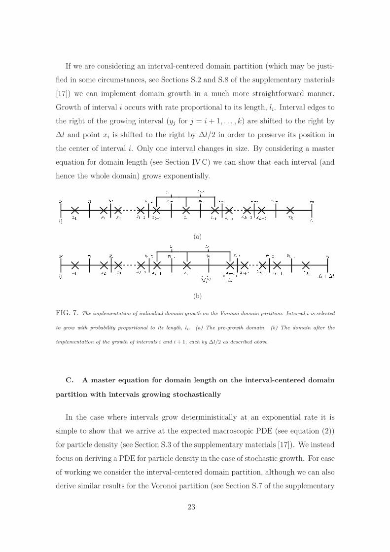
FIG. 7. The implementation of individual domain growth on the Voronoi domain partition. Interval i is selected

to grow with probability proportional to its length, li. (a) The pre-growth domain. (b) The domain after the

implementation of the growth of intervals i and i + 1, each by ∆l/2 as described above.

C. A master equation for domain length on the interval-centered domain

partition with intervals growing stochastically

In the case where intervals grow deterministically at an exponential rate it is

simple to show that we arrive at the expected macroscopic PDE (see equation (2))

for particle density (see Section S.3 of the supplementary materials [17]). We instead

focus on deriving a PDE for particle density in the case of stochastic growth. For ease

of working we consider the interval-centered domain partition, although we can also

derive similar results for the Voronoi partition (see Section S.7 of the supplementary

23

materials [17]). The interval-centered partition admits the possibility of individual

interval growth with rate proportional to interval length and simple interval division.

In addition it is possible to repartition the interval-centered domain in order to

calculate the particle densities which correspond to the mean-field PDE and, as

such, the interval-centered domain partition may be as valid as the Voronoi domain

partition for simulating particle migration on growing domains (see Section S.8 of

the supplementary materials [17]).

Consider a time interval small enough that the probability of more than one

growth event occurring in [t, t + δt) is O(δt) and ignore, for the meantime, the

movement of particles. Define L = (L1, . . . , Lk) to be the vector of random variables

representing the length of each interval. We express the probability that the jth

component of L, representing the length of interval j, takes the value lj at time

t + δt via the following master equation:

d Pr(L = l, t)

dt= r

k∑

i=1

Pr (L = (l1, . . . , li − ∆l, . . . , lk) , t) (li − ∆l)

− rk∑

i=1

li Pr(L = l, t), (44)

where l = (l1, . . . , lk) is the current state of the vector of interval length random

variables. In order to find the mean length of interval j we multiply through by

lj and sum over all the (finite number of) possible values that l can take. Upon

simplification we arrive at an ODE which describes how the mean of each interval

grows:

d 〈lj〉dt

= r∆l 〈lj〉 for j = 1, . . . , k, (45)

⇒ 〈lj〉 (t) = lj(0) exp(r∆lt) for j = 1, . . . , k, (46)

where lj(0) is the initial size of interval j. By taking the sum of ODEs (45) we can

arrive at an ODE for the average domain length, 〈L〉:d 〈L〉

dt= r∆l 〈L〉 , (47)

⇒ 〈L〉 (t) = L(0) exp(r∆lt), (48)

where L(0) =∑k

j=1 lj(0) is the original length of the domain.

24

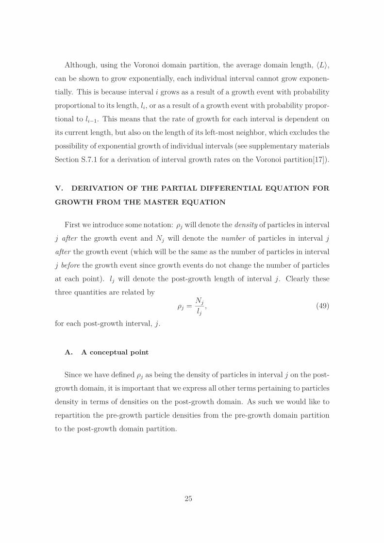
Although, using the Voronoi domain partition, the average domain length, 〈L〉,can be shown to grow exponentially, each individual interval cannot grow exponen-

tially. This is because interval i grows as a result of a growth event with probability

proportional to its length, li, or as a result of a growth event with probability propor-

tional to li−1. This means that the rate of growth for each interval is dependent on

its current length, but also on the length of its left-most neighbor, which excludes the

possibility of exponential growth of individual intervals (see supplementary materials

Section S.7.1 for a derivation of interval growth rates on the Voronoi partition[17]).

V. DERIVATION OF THE PARTIAL DIFFERENTIAL EQUATION FOR

GROWTH FROM THE MASTER EQUATION

First we introduce some notation: ρj will denote the density of particles in interval

j after the growth event and Nj will denote the number of particles in interval j

after the growth event (which will be the same as the number of particles in interval

j before the growth event since growth events do not change the number of particles

at each point). lj will denote the post-growth length of interval j. Clearly these

three quantities are related by

ρj =Nj

lj, (49)

for each post-growth interval, j.

A. A conceptual point

Since we have defined ρj as being the density of particles in interval j on the post-

growth domain, it is important that we express all other terms pertaining to particles

density in terms of densities on the post-growth domain. As such we would like to

repartition the pre-growth particle densities from the pre-growth domain partition

to the post-growth domain partition.

25

B. Pre-growth densities on the post-growth domain partition

To repartition particles from the pre-growth domain to the post-growth domain

we must first repartition the pre-growth particle numbers on the pre-growth domain

partition, denoted by the vector N , to the post-growth domain partition. This

repartitioned vector will be denoted N ′. Since the pre- and post-growth domain

partitions are the same up to the interval i, which grows, we have N ′j = Nj for j < i.

Since interval i grows, the number of particle in the pre-growth domain that lie in the

post-growth interval i is N ′i = Ni+Ni+1∆l/li+1. This corresponds to all the particles

that lie in the pre-growth interval i added to the fraction ∆l/li+1 of the particles

which lie in the pre-growth interval i+1, Ni+1. This fraction ( ∆l/li+1) is the amount

of overlap between the post-growth interval i and the pre-growth interval i + 1 and

our repartitioning assumes particles are spread homogeneously across each interval.

In a similar manner, the number of particles in the pre-growth domain that lie in

post-growth interval j > i is N ′j = Nj (1 − ∆l/lj)+(∆l/lj+1) Nj+1. The factor ∆l/lj

corresponds to the fraction of particles in pre-growth interval j lost to post-growth

interval j − 1 (hence 1 − ∆l/lj corresponds to the fraction of particles in pre-growth

interval j that are also in post-growth interval j). Correspondingly ∆l/lj+1 is the

number of particles requisitioned by post-growth interval j from pre-growth interval

j + 1 (see Fig. 8). Finally, the number of particles that lie in post-growth interval k

is N ′k = Nk (1 − ∆l/lk), where 1 − ∆l/lk represents the overlap fraction of pre- and

post-growth intervals, k.

Now that we have repartitioned the particle numbers to the post-growth domain

partition, it is a simple matter to find the pre-growth densities on the post-growth

domain partition, qj. For all j < i we have

qj =Nj

lj= ρj, (50)

since the boundaries of these intervals are the same on the post- and pre-growth

domain partition (see Fig. 8). For j = i:

qi =Ni + Ni+1 (∆l/li+1)

li= ρi +

∆l

liρi+1. (51)

Similarly, if i < j < k then we can write the pre-growth densities on the post-growth

26

(a)

(b)

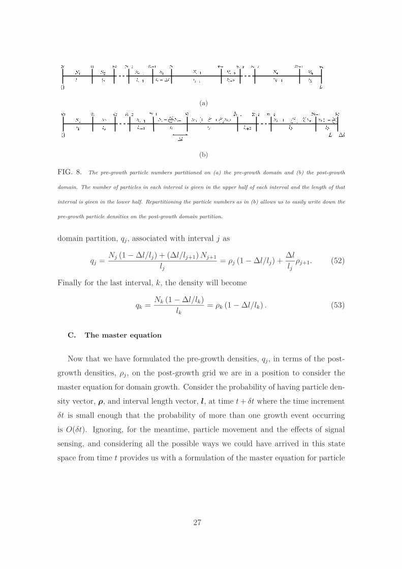
FIG. 8. The pre-growth particle numbers partitioned on (a) the pre-growth domain and (b) the post-growth

domain. The number of particles in each interval is given in the upper half of each interval and the length of that

interval is given in the lower half. Repartitioning the particle numbers as in (b) allows us to easily write down the

pre-growth particle densities on the post-growth domain partition.

domain partition, qj, associated with interval j as

qj =Nj (1 − ∆l/lj) + (∆l/lj+1) Nj+1

lj= ρj (1 − ∆l/lj) +

∆l

ljρj+1. (52)

Finally for the last interval, k, the density will become

qk =Nk (1 − ∆l/lk)

lk= ρk (1 − ∆l/lk) . (53)

C. The master equation

Now that we have formulated the pre-growth densities, qj, in terms of the post-

growth densities, ρj, on the post-growth grid we are in a position to consider the

master equation for domain growth. Consider the probability of having particle den-

sity vector, ρ, and interval length vector, l, at time t + δt where the time increment

δt is small enough that the probability of more than one growth event occurring

is O(δt). Ignoring, for the meantime, particle movement and the effects of signal

sensing, and considering all the possible ways we could have arrived in this state

space from time t provides us with a formulation of the master equation for particle

27

density on a growing domain:

∂ Pr(ρ, l, t)

∂t= r

k∑

i=1

Pr(q1, . . . , qi, qi+1, . . . , qk, l1, . . . , li − ∆l, . . . , lk, t) (li − ∆l)

− rk∑

i=1

Pr(ρ, l, t)li. (54)

Multiplying through by the particle density in interval j, ρj, and summing over all

the possible values that particle density can take we arrive at

∂ 〈ρj〉∂t

= rk∑

i=1

∑

ρρj Pr(q1, . . . , qi, qi+1, . . . , qk, l1, . . . , li − ∆l, . . . , lk, t) (li − ∆l)

− rk∑

i=1

〈ρjli〉 , (55)

where 〈ρj〉 =∑

ρ ρj Pr(ρ, l, t) represents the mean number of particles in interval j

and 〈ρjli〉 =∑

ρ ρjli Pr(ρ, l, t). Note that values that particle density can take are

determined by the number of particles in the interval and the width of that interval.

Therefore, in the above equation and elsewhere, we use the shorthand notation,∑

ρ, to represent the double sum over all possible particle numbers and all possible

interval widths,∑

N∑

l. For the first sum on the right-hand side of equation (55)

we must carefully consider each value of i. For i > j the terms are of the form

r∑

ρρj Pr(q1, . . . , qi, qi+1, . . . , qk, l1, . . . , li − ∆l, . . . , lk, t) (li − ∆l) = r 〈ρjli〉 , (56)

since qj = ρj for j < i. However, if i ≤ j then the growth event occurs at, or to the

left of, interval j and things are not so simple.

For j = i:

r∑

ρρj Pr

(

ρ1, . . . , ρj−1, ρj +∆l

ljρj+1, ρj+1

(

1 − ∆l

lj+1

)

+∆l

lj+1ρj+2, . . . , ρk (1 − ∆l/lk) ,

l1, . . . , lj − ∆l, . . . , lk, t

)

(lj − ∆l)

= r∑

ρ

(

ρj +∆l

ljρj+1

)

Pr

(

ρ1, . . . , ρj−1, ρj +∆l

ljρj+1, ρj+1

(

1 − ∆l

lj+1

)

+∆l

lj+1

ρj+2, . . . ,

ρk (1 − ∆l/lk) , l1, . . . , lj − ∆l, . . . , lk, t

)

(lj − ∆l)

− r∑

ρ

∆l

ljρj+1 Pr

(

ρ1, . . . , ρj−1, ρj +∆l

ljρj+1, ρj+1

(

1 − ∆l

lj+1

)

+∆l

lj+1ρj+2, . . . ,

28

ρk (1 − ∆l/lk) , l1, . . . , lj − ∆l, . . . , lk, t

)

(lj − ∆l)

= r 〈ρjlj〉 − r∑

ρ

∆l

lj

(

lj+1

lj+1 − ∆l

)

ρj+1

(

1 − ∆l

lj+1

)

+∆l

lj+1

ρj+2

Pr

(

ρ1, . . . , ρj−1, ρj +∆l

ljρj+1,

ρj+1

(

1 − ∆l

lj+1

)

+∆l

lj+1

ρj+2, . . . , ρk (1 − ∆l/lk) , l1, . . . , lj − ∆l, . . . , lk, t

)

(lj − ∆l) + O(∆l2)

= r 〈ρjlj〉 − r∆l 〈ρj+1〉 + O(∆l2). (57)

To go between the first and second equality in this statement we have added and

subtracted terms that are O(∆l2), namely:

r∑

ρ

∆l

lj

(

lj+1

lj+1 − ∆l

)

∆l

lj+1ρj+2 Pr(. . . ) (lj − ∆l) , (58)

where the term we have added is incorporated into the O(∆l2) term. To go between

the second and third equalities we have used the Taylor expansion of 1/(lj+1 − ∆l)

and grouped all O(∆l2) terms together:

1

lj+1 − ∆l=

1

lj+1

+∆l

(lj+1)2+ O(∆l2), (59)

so that ∆l(lj+1/(lj+1 − ∆l)) may be approximated by ∆l + O(∆l2). We have also

made use of the following Taylor expansion of 1/lj:

1

lj=

1

(lj − ∆l) + ∆l=

1

lj − ∆l− ∆l

(lj − ∆l)2 + O(∆l2), (60)

so that ∆l/lj may be approximated as ∆l/ (lj − ∆l) + O(∆l2).

In general, for 1 ≤ i < j all terms will take a similar form:

r∑

ρρj Pr

(

q1, . . . , qj−1, ρj (1 − ∆l/lj) +∆l

ljρj+1, ρj+1 (1 − ∆l/lj+1) +

∆l

lj+1

ρj+2, . . . ,

ρk (1 − ∆l/lk) , l1, . . . , li − ∆l, . . . , lk, t

)

(li − ∆l)

= r∑

ρ

(

ljlj − ∆l

)(

ρj (1 − ∆l/lj) +∆l

ljρj+1

)

Pr

(

q1, . . . , qj−1, ρj (1 − ∆l/lj) +∆l

ljρj+1,

ρj+1 (1 − ∆l/lj+1) +∆l

lj+1

ρj+2, . . . , ρk (1 − ∆l/lk) , l1, . . . , li − ∆l, . . . , lk, t

)

(li − ∆l)

− r∑

ρ

(

∆l

lj − ∆l

)

ρj+1 Pr

(

q1, . . . , qj−1, ρj (1 − ∆l/lj) +∆l

ljρj+1, ρj+1 (1 − ∆l/lj+1) +

∆l

lj+1ρj+2,

29

. . . , ρk (1 − ∆l/lk) , l1, . . . , li − ∆l, . . . , lk, t

)

(li − ∆l)

= r∑

ρ

(

1 +∆l

lj − ∆l

)(

ρj (1 − ∆l/lj) +∆l

ljρj+1

)

Pr

(

q1, . . . , qj−1, ρj (1 − ∆l/lj) +∆l

ljρj+1,

ρj+1 (1 − ∆l/lj+1) +∆l

lj+1

ρj+2, . . . , ρk (1 − ∆l/lk) , l1, . . . , li − ∆l, . . . , lk, t

)

(li − ∆l)

− r∑

ρ

(

∆l

lj − ∆l

)(

lj+1

lj+1 − ∆l

)

ρj+1

(

1 − ∆l

lj+1

)

+∆l

lj+1ρj+2

Pr

(

q1, . . . , qj−1,

ρj (1 − ∆l/lj) +∆l

ljρj+1, ρj+1 (1 − ∆l/lj+1) +

∆l

lj+1ρj+2, . . . , ρk (1 − ∆l/lk) , l1,

. . . , li − ∆l, . . . , lk, t

)

(li − ∆l) + O(∆l2)

= r 〈ρjli〉 + r∆l

⟨

ρjlilj

⟩

− r∆l

⟨

ρj+1lilj

⟩

+ O(∆l2). (61)

Again, to arrive at the last equality we have used a Taylor expansion of 1/(lj − ∆l):

1

lj − ∆l=

1

lj+ ∆l

1

(lj)2+ O(∆l2), (62)

and the Taylor expansion of 1/(lj+1 − ∆l) from the case i = j, above. We substitute

the expressions from equations (56), (57) and (61) into the right-hand side of the

master equation (55):

∂ 〈ρj〉∂t

= rk∑

i=1

〈ρjli〉 − rk∑

i=1

〈ρjli〉

+ r∆lj−1∑

i=1

⟨

ρjlilj

⟩

−⟨

ρj+1lilj

⟩

+ r∆l

⟨

ρjljlj

⟩

− r∆l

⟨

ρj+1ljlj

⟩

− r∆l 〈ρj〉 + O(∆l2), (63)

where we have added and subtracted r∆l 〈ρjlj/lj〉 = r∆l 〈ρj〉 to the right-hand side.

This can be written more simply as:

∂ 〈ρj〉∂t

= −r∆l 〈ρj〉 − r∆lj∑

i=1

(⟨

ρj+1lilj

⟩

−⟨

ρjlilj

⟩)

. (64)

We make a moment closure approximation in order to make these terms manageable.

To do this we assume:⟨

ρjlilj

⟩

=〈ρj〉〈li〉

〈lj〉. (65)

30

We justify the use of this moment closure approximation using numerical simulations

in Section VI C. Upon applying this moment closure approximation we can re-write

equation (64) as∂ 〈ρj〉

∂t= −r∆l 〈ρj〉 − xr∆l

〈ρj+1〉 − 〈ρj〉〈lj〉

, (66)

where we have recognized that∑j

i=1 〈li〉 = x. Taylor expanding the term ρj+1 and

taking the limit of the interval sizes tending to zero (note that in order to maintain

a constant rate of domain growth, as lj → 0, we allow ∆l → 0 in such a way that

r∆l remains constant) i.e. lj → 0 yields a PDE formulation:

∂u

∂t= D

∂2u

∂x2− r∆lu − xr∆l

∂u

∂x, (67)

for particle density, u = u(x, t), where we have reintroduced terms due to particle

movement since their inclusion does not affect the derivation of the domain growth

terms.

These are precisely the terms we would expect, as per equation (2), when consid-

ering exponential domain growth. The term r∆l 〈ρj〉 corresponds to local dilution

due to volume increase and xr∆l∂ 〈ρj〉 /∂x corresponds to material being trans-

ported along the domain by the flow induced by growth.

Here we have derived a PDE for the mean density, 〈ρj〉 = 〈Nj/lj〉. It should

be noted that it may be simpler to derive a PDE for the mean number of particles

in each interval divided by the mean interval length 〈Nj〉 / 〈lj〉, which can in some

senses be thought to be the mean density. Such a derivation for the interval-centered

domain partition is given in Section S.3 of the supplementary materials [17]).

The derivation of the PDE on the Voronoi domain is similar to that of the PDE

on the interval-centered domain partition, illustrated above, and is given in Section

S.7.2 of the supplementary materials [17]). As we have already hinted, the PDE

derived for the Voronoi domain partition is similar to, but not exactly the same

as, the PDE derived above for the interval-centered partition. This is because the

domain growth is not uniformly exponential across each interval of the Voronoi

domain partition.

31

VI. NUMERICAL SIMULATIONS

To corroborate our findings we have carried out extensive numerical simulations

using different domain growth mechanisms and interval partitions.

We note the difficulty in representing average particle densities over several re-

peats: in the stochastic implementations of domain growth the partition of the

domain in each of the repeat simulations will be different. In the deterministic

implementations of domain growth (see Section IV A) all the intervals grow at the

same rate implying that the domain partition should be the same at all the sampled

time points. However, due to the stochastic nature of the particle movement and

the time-step chosen for each reaction, simulations cannot be sampled with exactly

the same domain partition. These factors require us to rethink what we mean by

average particle density. To circumvent this problem we define a uniform mesh over

the domain and redistribute particle density into these regions at time-points where

we wish to record the density. This relies on the assumption that particles are spread

homogeneously across each interval.

A. Particles diffusing on an initially uniform domain partition with deter-

ministic exponential interval growth

In Fig. 9 we implement deterministic domain growth on an initially uniform do-

main partition, as described in Section IV A. In this case the interval-centered and

Voronoi domain partitions are equivalent. Particle densities in both the stochastic

and PDE models are found to match well, as evidenced quantitatively by the evo-

lution of the histogram distance error with time (see Fig. 9 (f)). Note that in all

the histogram distance error figures in this manuscript, when particles are initial-

ized in the first interval the error starts off large as an artifact of the way we are

forced to initialize our PDE to replicate this condition. When we initialize with an

exponentially decaying profile of particles (see Fig. S.1 in the supplementary mate-

rials [17]) for example) we do not see this initial disparity since this initial profile is

straightforward to replicate in the continuum model.

The domain in the individual-level model grows, on average, at the same rate as

32

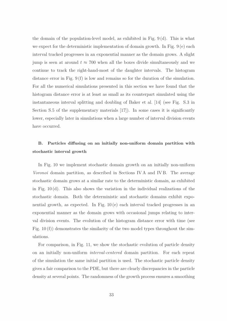
the domain of the population-level model, as exhibited in Fig. 9 (d). This is what

we expect for the deterministic implementation of domain growth. In Fig. 9 (e) each

interval tracked progresses in an exponential manner as the domain grows. A slight

jump is seen at around t ≈ 700 when all the boxes divide simultaneously and we

continue to track the right-hand-most of the daughter intervals. The histogram

distance error in Fig. 9 (f) is low and remains so for the duration of the simulation.

For all the numerical simulations presented in this section we have found that the

histogram distance error is at least as small as its counterpart simulated using the

instantaneous interval splitting and doubling of Baker et al. [14] (see Fig. S.3 in

Section S.5 of the supplementary materials [17]). In some cases it is significantly

lower, especially later in simulations when a large number of interval division events

have occurred.

B. Particles diffusing on an initially non-uniform domain partition with

stochastic interval growth

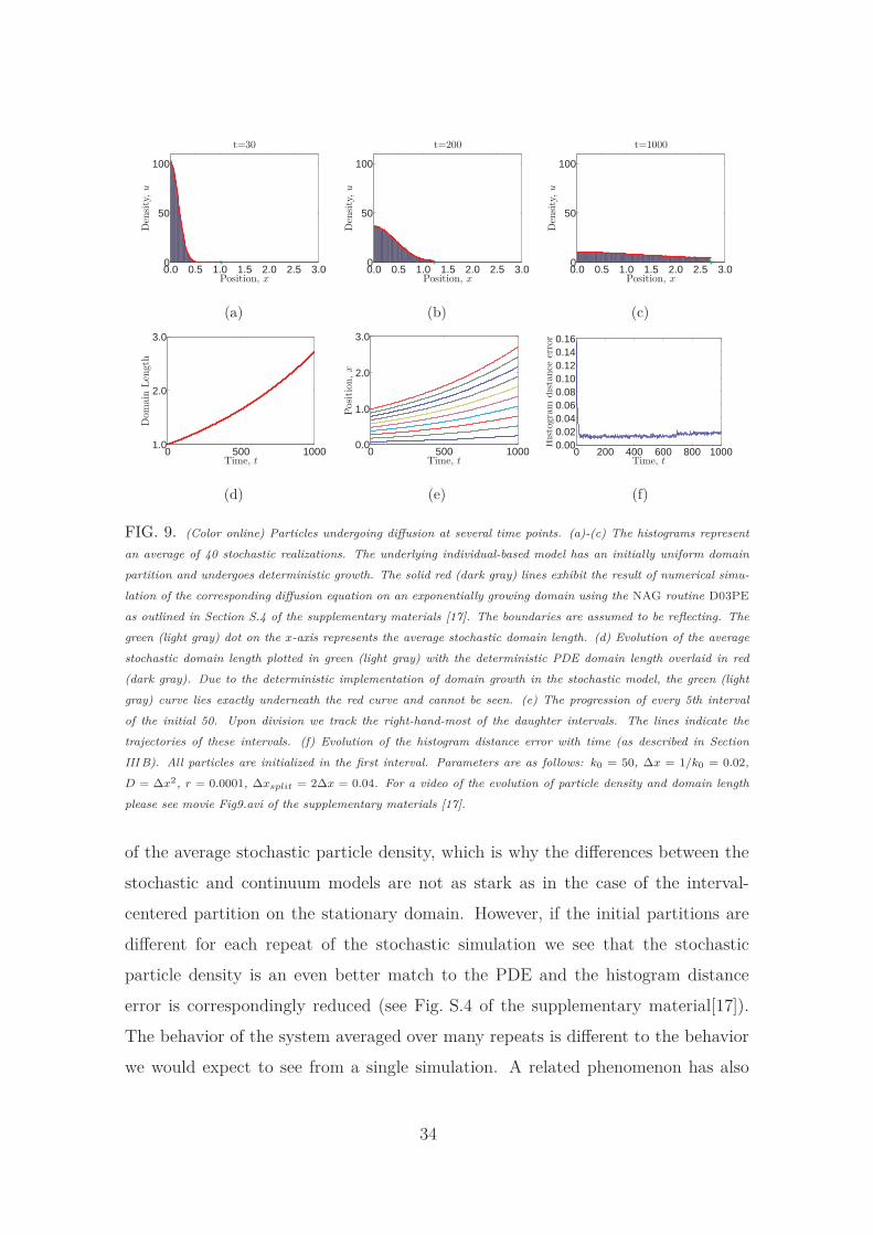
In Fig. 10 we implement stochastic domain growth on an initially non-uniform

Voronoi domain partition, as described in Sections IV A and IV B. The average

stochastic domain grows at a similar rate to the deterministic domain, as exhibited

in Fig. 10 (d). This also shows the variation in the individual realizations of the

stochastic domain. Both the deterministic and stochastic domains exhibit expo-

nential growth, as expected. In Fig. 10 (e) each interval tracked progresses in an

exponential manner as the domain grows with occasional jumps relating to inter-

val division events. The evolution of the histogram distance error with time (see

Fig. 10 (f)) demonstrates the similarity of the two model types throughout the sim-

ulations.

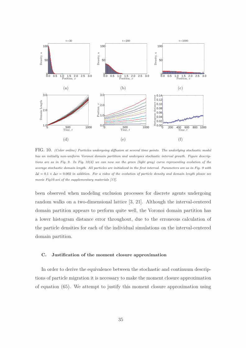
For comparison, in Fig. 11, we show the stochastic evolution of particle density

on an initially non-uniform interval-centered domain partition. For each repeat

of the simulation the same initial partition is used. The stochastic particle density

gives a fair comparison to the PDE, but there are clearly discrepancies in the particle

density at several points. The randomness of the growth process ensures a smoothing

33

0.0 0.5 1.0 1.5 2.0 2.5 3.00

50

100

Position, x

Density,u

t=30

(a)

0.0 0.5 1.0 1.5 2.0 2.5 3.00

50

100

Position, x

Density,u

t=200

(b)

0.0 0.5 1.0 1.5 2.0 2.5 3.00

50

100

Position, x

Density,u

t=1000

(c)

0 500 10001.0

2.0

3.0

Time, t

Domain

Length

(d)

0 500 10000.0

1.0

2.0

3.0

Time, t

Position,x

(e)

0 200 400 600 800 10000.000.020.040.060.080.100.120.140.16

Time, t

Histogram

distance

error

(f)

FIG. 9. (Color online) Particles undergoing diffusion at several time points. (a)-(c) The histograms represent

an average of 40 stochastic realizations. The underlying individual-based model has an initially uniform domain

partition and undergoes deterministic growth. The solid red (dark gray) lines exhibit the result of numerical simu-

lation of the corresponding diffusion equation on an exponentially growing domain using the NAG routine D03PE

as outlined in Section S.4 of the supplementary materials [17]. The boundaries are assumed to be reflecting. The

green (light gray) dot on the x-axis represents the average stochastic domain length. (d) Evolution of the average

stochastic domain length plotted in green (light gray) with the deterministic PDE domain length overlaid in red

(dark gray). Due to the deterministic implementation of domain growth in the stochastic model, the green (light

gray) curve lies exactly underneath the red curve and cannot be seen. (e) The progression of every 5th interval

of the initial 50. Upon division we track the right-hand-most of the daughter intervals. The lines indicate the

trajectories of these intervals. (f) Evolution of the histogram distance error with time (as described in Section

III B). All particles are initialized in the first interval. Parameters are as follows: k0 = 50, ∆x = 1/k0 = 0.02,

D = ∆x2, r = 0.0001, ∆xsplit = 2∆x = 0.04. For a video of the evolution of particle density and domain length

please see movie Fig9.avi of the supplementary materials [17].

of the average stochastic particle density, which is why the differences between the

stochastic and continuum models are not as stark as in the case of the interval-

centered partition on the stationary domain. However, if the initial partitions are

different for each repeat of the stochastic simulation we see that the stochastic

particle density is an even better match to the PDE and the histogram distance

error is correspondingly reduced (see Fig. S.4 of the supplementary material[17]).

The behavior of the system averaged over many repeats is different to the behavior

we would expect to see from a single simulation. A related phenomenon has also

34

0.0 0.5 1.0 1.5 2.0 2.5 3.00

50

100

Position, x

Density,u

t=30

(a)

0.0 0.5 1.0 1.5 2.0 2.5 3.00

50

100

Position, x

Density,u

t=200

(b)

0.0 0.5 1.0 1.5 2.0 2.5 3.00

50

100

Position, x

Density,u

t=1000

(c)

0 500 10001.0

2.0

3.0

Time, t

Domain

Length

(d)

0 500 10000.0

1.0

2.0

3.0

Time, t

Position,x

(e)

0 200 400 600 800 10000.00

0.02

0.04

0.06

0.08

0.10

0.12

0.14

Time, t

Histogram

distance

error

(f)

FIG. 10. (Color online) Particles undergoing diffusion at several time points. The underlying stochastic model

has an initially non-uniform Voronoi domain partition and undergoes stochastic interval growth. Figure descrip-

tions are as in Fig. 9. In Fig. 10(d) we can now see the green (light gray) curve representing evolution of the

average stochastic domain length. All particles are initialized in the first interval. Parameters are as in Fig. 9 with

∆l = 0.1 × ∆x = 0.002 in addition. For a video of the evolution of particle density and domain length please see

movie Fig10.avi of the supplementary materials [17].

been observed when modeling exclusion processes for discrete agents undergoing

random walks on a two-dimensional lattice [3, 21]. Although the interval-centered

domain partition appears to perform quite well, the Voronoi domain partition has

a lower histogram distance error throughout, due to the erroneous calculation of

the particle densities for each of the individual simulations on the interval-centered

domain partition.

C. Justification of the moment closure approximation

In order to derive the equivalence between the stochastic and continuum descrip-

tions of particle migration it is necessary to make the moment closure approximation

of equation (65). We attempt to justify this moment closure approximation using

35

0.0 0.5 1.0 1.5 2.0 2.5 3.00

50

100

Position, x

Density,u

t=30

(a)

0.0 0.5 1.0 1.5 2.0 2.5 3.00

50

100

Position, x

Density,u

t=200

(b)

0.0 0.5 1.0 1.5 2.0 2.5 3.00

50

100

Position, x

Density,u

t=1000

(c)

0 500 10001.0

2.0

3.0

Time, t

Domain

Length

(d)

0 500 10000.0

1.0

2.0

3.0

Time, t

Position,x

(e)

0 200 400 600 800 10000.02

0.04

0.06

0.08

0.10

0.12

0.14

Time, t

Histogram

distance

error

(f)

FIG. 11. (Color online) Particles undergoing diffusion at several time points. The underlying stochastic model

has an initially non-uniform interval-centered domain partition and undergoes stochastic interval growth. All

repeats are initialized with the same domain partition. Figure descriptions are as in Figs. 9 and 10. All particles

are initialized in the first interval. Parameters are as in Fig. 10. For a video of the evolution of particle density

and domain length please see movie Fig11.avi of the supplementary materials [17].

the results of our stochastic simulations by plotting(⟨

ρjlilj

⟩

− 〈ρj〉〈li〉〈lj〉

)/⟨

ρjlilj

⟩

, (68)

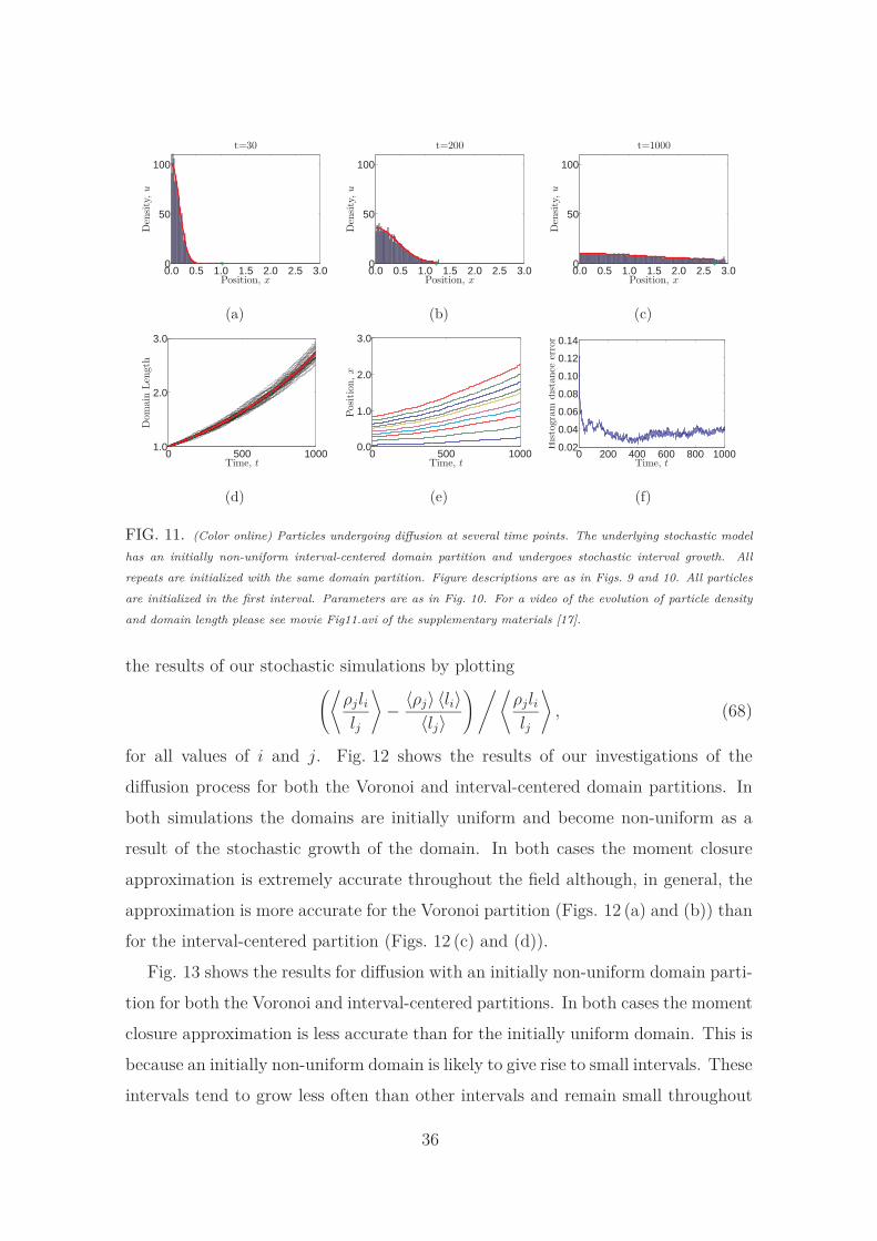
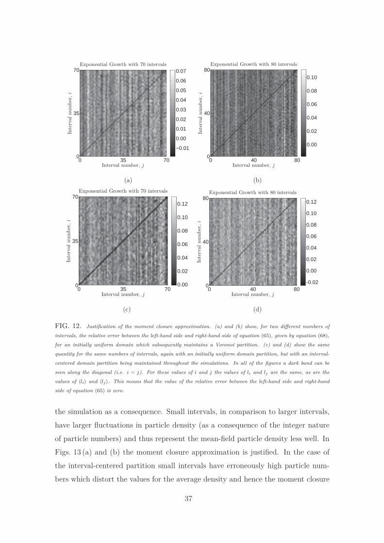
for all values of i and j. Fig. 12 shows the results of our investigations of the

diffusion process for both the Voronoi and interval-centered domain partitions. In

both simulations the domains are initially uniform and become non-uniform as a

result of the stochastic growth of the domain. In both cases the moment closure

approximation is extremely accurate throughout the field although, in general, the

approximation is more accurate for the Voronoi partition (Figs. 12 (a) and (b)) than

for the interval-centered partition (Figs. 12 (c) and (d)).

Fig. 13 shows the results for diffusion with an initially non-uniform domain parti-

tion for both the Voronoi and interval-centered partitions. In both cases the moment

closure approximation is less accurate than for the initially uniform domain. This is

because an initially non-uniform domain is likely to give rise to small intervals. These

intervals tend to grow less often than other intervals and remain small throughout

36

Interval number, j

Inte

rvalnum

ber

,i

Exponential Growth with 70 intervals

0 35 70

70

35

0

−0.01

0.00

0.01

0.02

0.03

0.04

0.05

0.06

0.07

(a)

Interval number, j

Inte

rvalnum

ber

,i


0 40 80

80

40

0

0.00

0.02

0.04

0.06

0.08

0.10

(b)

Interval number, j

Intervalnumber,i


0 35 70

70

35

0 0.00

0.02

0.04

0.06

0.08

0.10

0.12

(c)

Interval number, j

Intervalnumber,i


0 40 80

80

40

0-0.02

0.00

0.02

0.04

0.06

0.08

0.10

0.12

(d)

FIG. 12. Justification of the moment closure approximation. (a) and (b) show, for two different numbers of

intervals, the relative error between the left-hand side and right-hand side of equation (65), given by equation (68),

for an initially uniform domain which subsequently maintains a Voronoi partition. (c) and (d) show the same

quantity for the same numbers of intervals, again with an initially uniform domain partition, but with an interval-

centered domain partition being maintained throughout the simulations. In all of the figures a dark band can be

seen along the diagonal (i.e. i = j). For these values of i and j the values of li and lj are the same, as are the

values of 〈li〉 and 〈lj〉. This means that the value of the relative error between the left-hand side and right-hand

side of equation (65) is zero.

the simulation as a consequence. Small intervals, in comparison to larger intervals,

have larger fluctuations in particle density (as a consequence of the integer nature

of particle numbers) and thus represent the mean-field particle density less well. In

Figs. 13 (a) and (b) the moment closure approximation is justified. In the case of

the interval-centered partition small intervals have erroneously high particle num-

bers which distort the values for the average density and hence the moment closure

37

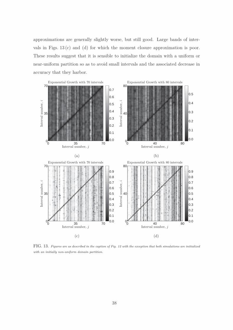
approximations are generally slightly worse, but still good. Large bands of inter-

vals in Figs. 13 (c) and (d) for which the moment closure approximation is poor.

These results suggest that it is sensible to initialize the domain with a uniform or

near-uniform partition so as to avoid small intervals and the associated decrease in

accuracy that they harbor.

Interval number, j

Intervalnumber,i


0 35 70

70

35

0 0.0

0.1

0.2

0.3

0.4

0.5

0.6

0.7

(a)

Interval number, j

Intervalnumber,i


0 40 80

80

40

0 0.0

0.1

0.2

0.3

0.4

0.5

(b)

Interval number, j

Intervalnumber,i


0 35 70

70

35

0 0.0

0.1

0.2

0.3

0.4

0.5

0.6

0.7

0.8

0.9

(c)

Interval number, j

Intervalnumber,i


0 40 80

80

40

0 0.0

0.1

0.2

0.3

0.4

0.5

0.6

0.7

0.8

0.9

(d)

FIG. 13. Figures are as described in the caption of Fig. 12 with the exception that both simulations are initialized

with an initially non-uniform domain partition.

38

VII. CONCLUSIONS

A. Summary

We began this work, in Section II, by summarizing a stochastic position-jump

framework for considering particle movement on an regular domain partition and

demonstrated, via a continuous time RDME describing probability density, that the

evolution of the mean density of particles in each interval can be linked to a PDE

using a Taylor series expansion to convert from discrete space to continuous space.

In Section III we generalized these results to a stochastic framework in which the

domain partition was no longer uniform. In order to derive transition rates between

non-uniform intervals we solved the first passage problem for an underlying micro-

scopic process defined by an SDE and corresponding FPE. The derived transition

rates were found to be a generalization of the transition rates on the uniform domain

partition. Numerical simulations were used to confirm the validity of our results.

Developing this equivalence framework between discrete microscale processes and

continuum macroscale processes is important as it potentially allows us to base our

models on experimental observations at an individual level and also to derive an

equivalent description at the level of the whole population. These models provide

us with a tool which is capable of representing both global and individual-level

properties. Individual-level models are compatible with the incorporation of micro-

scopic experimental data whilst the macroscopic PDE models allow us to extort the

wide range of analytical tools available and to analyze the global properties of such

models.

The main motivation for the consideration of non-uniform domain partitions was

a more physically reasonable incorporation of domain growth into position-jump

models than has previously been presented [14]. Instead of allowing intervals to

instantaneously double in size and divide, in Section IV, we made growth a more

continuous process and loosened the coupling between interval growth and interval

division, with intervals dividing only upon reaching a certain size. As a toy model we

introduced deterministic domain growth in order to verify that domain growth could

be implemented in an incremental fashion. However, we derived our main result,

39

pertaining to stochastic, incremental domain growth in Section V. We used a master

equation formalism to show that the stochastic process of domain growth introduced

in Section IV was equivalent to a classic PDE describing continuous exponential

domain growth under some mild moment closure assumptions. We justified these

assumptions, in Section VI, as well as corroborating our theoretical derivations with

numerical simulations demonstrating the qualitative and quantitative equivalence of

the stochastic and continuum models for diffusion.

B. Discussion

Position-jump models, like the ones considered in this paper, are by no means

the only individual-based models from which continuum models for particle density

can be derived. Bodnar and Velazquez [22] and Murray et al. [23] derive continuum

versions of off-lattice individual-based models in one dimension.

Bellomo et al. [24] provide a useful overview of the use of asymptotic theory

to transition from microscopic to macroscopic descriptions of particle migration,

where the fundamental microscopic model employed is the velocity-jump process

investigated in [8, 12, 13].

Considering on-lattice, individual-based models, it is often possible to write down

a probability master equation describing the evolution of the probability that a

system is in a certain state. Turner et al. [9] use the probability master equation

on a one-dimensional cellular Potts model incorporating inter-individual adhesion in

order to derive a linear diffusion equation whose diffusion coefficient can be linked

explicitly to the model parameters. Alber et al. [10] extend this work into two

dimensions.

The individual-level models which allow for the most straightforward derivation

of a continuum limit are, like the models presented in this paper, on-lattice, position-

jump models. Individuals are assumed to be points particles (as opposed to having

finite size as in the cellular Potts model) and are restricted to (local) movement to

one of their neighboring lattice sites with prescribed, possibly signal mediated, tran-

sition rates. Elementary examples of such discrete-continuum equivalence frame-

40

works based on simple random walk models can be found in the influential texts

of Berg [25] and Lin and Segel [26]. Codling et al. [27] also provides an overview

of the derivation of continuum models of both biased and unbiased position-jump

(or uncorrelated) random walks, as well as their velocity-jump (or correlated) coun-

terparts. Other authors who have dealt with on-lattice individual-based models via

the reaction-diffusion master equation formalism approach adopted in this paper

include Isaacson [28], Drawert et al. [29] and Ferm et al. [30].

The canonical model on which our work is founded is the position-jump (or

‘kangaroo’ as they refer to it) model of Othmer et al. [8]. They are able to derive

a continuum limit by considering an appropriate probability master equation and

show, with a special choice of the jump kernel (so that only unbiased, discrete jumps

of size ∆ are allowed), that the continuum equation reduces to the diffusion equation.

At present we do not consider interactions between particles in our model. Painter

and Hillen [2], however, do incorporate particle interaction into the transition rates

of their on-lattice, individual-based model. Upon taking the continuum limit, in a

similar manner to Othmer and Stevens [1], they arrive at a system of Keller-Segel-

like equations.

The discrete-continuum equivalence frameworks on the stationary domain, built

up in the above mentioned works, have inspired us to ask questions about how to

appropriately incorporate domain growth into such frameworks. Domain growth

has been successfully included in models of particle migration and such models have

been used to demonstrate peak insertion and splitting in fish skin patterning [31, 32].

Adapted chemotaxis models with volume filling have also been used to show that

peak insertion or splitting is not a necessary result of pattern formation on a growing

domain [2]. Using similar PDE models Landman et al. [33] study a population of

cells chemotaxing on a growing domain.

Despite these successes in a continuum setting the realistic incorporation of do-

main growth into on-lattice, individual-level position-jump models has not previ-

ously been elucidated. In this paper we have built directly on our previous work,

[14], by attempting to make the method of domain growth in the individual model

more physically reasonable. We combined a basic position-jump type model with a

41

novel domain growth method which allows the underlying lattice elements to grow

incrementally. Using a further adapted master equation-type formalism we were able

to derive a continuum equivalent to our model. Our numerical simulations demon-

strate that this new method of domain growth tends to make our individual-based

models more similar to their continuum counterparts than our previous method.

Despite the advances made in this current work there remain a multitude of

related open problems.

C. Open problems

There are several possible avenues for further research. Firstly, the domain parti-

tion dichotomy between the Voronoi and the interval-centered domain partitions is

by no means perfect. It is obvious that on the stationary domain we should use the

Voronoi partition to ensure the correct density of particles in each interval. However,

on the growing domain we cannot derive a closed-form PDE for cell density with the

Voronoi partition due to the enforced nature of interval growth: two intervals must

grow at the same time in order to preserve the Voronoi property of the domain,

thus preventing each interval from growing exponentially. We have demonstrated

that the interval-centered domain partition allows us to derive a master equation

which corresponds closely with the expected PDE for particle density on the growing

domain. We have also seen, however, that the particle densities on this partition

will, ultimately, not correspond to the mean-field densities. This poses a question as

to whether some sort of domain partition duality might be more appropriate. The

interval-centered domain partition may be employed to ensure the correct interval

growth rates and the Voronoi domain partition used in order to find the correct par-

ticle densities (see Figs. S.5 and S.6 of the supplementary materials [17]. Each time

we require particle density it would be simple enough, keeping interval centers as

fixed points, to find the corresponding Voronoi domain partition on which we might

expect particle density to be correct. This, does, however, pose questions as to what

exactly we mean by particle density. Even more troubling, from a computational

point of view, is the situation in which particle migration or domain growth are

42

dependent on density. This would require conversion from the interval-centered to

the Voronoi domain partition at every time-step which would surely lead to a large

increase in simulation times.

Secondly, the question of robust pattern formation for stochastic processes on

growing domains is one of much biological and mathematical interest [34, 35]. Un-

til now there has been no method to simulate such stochastic processes robustly,

without artificially changing the nature of the pattern formed by implementing in-

stantaneous ‘growth and division’ events. We envisage that our new incremental

interval growth method, and its corresponding PDE, will be of great interest to

mathematicians and biologists alike, allowing for the correct simulation of stochas-

tic pattern formation and evolution even with strong ubiquitous growth.

Thirdly, the two way coupling between particle migration and tissue growth is

important from a biological point of view. Not only does growth affect the move-

ment of the particles on the domain, but the particles can also feed back and affect

growth of the domain [15, 36]. In our previous work, Baker et al. [14] we were able

to incorporate different mechanisms of domain growth (including density-dependent

growth) into our discrete-continuum equivalence framework. This has yet to be ac-

complished for our more physically reasonable method of domain growth but, given

the insights gained in this paper with regards to the necessity of the Voronoi domain

partition for the calculation of the correct particle densities, we have provided the

platform to make this possible.

Finally, we have yet to apply the domain growth modeling work presented in

this paper to experimental systems. There are many possibilities which we might

consider. Kruse [16] presents an initially individual-based one-dimensional position-

jump model for the localization of the division septum in dividing Escherichia coli

bacterial cells. As an approximation, the time-scale of the localization is assumed to

be fast in comparison to the time-scale of growth and hence the effects of growth are

neglected. Our modeling regime would potentially allow for the effects of domain

growth on the localization of the division septum to be explored in the context of

Kruse’s model.

The goal of our research is to provide insights into the mechanisms underlying

43

the movement of individuals (be they inert particles, proteins or cells) on growing

domains. The work of Kruse [16] is just one of many potential applications of

the modeling regime we have presented in this paper. It seems prudent that, in

applying our modeling paradigm to biological situations, further model analysis

and parametrization, followed by repeats of the “alter-predict-test” cycle should be

carried out in order to suggest ways in which the models should be improved.

Acknowledgements

CAY would like to thank Christ Church College for a Junior Research Fellowship.

RE would also like to thank Somerville College, University of Oxford for Fulford

Junior Research Fellowship. The research leading to these results has received fund-

ing from the European Research Council under the European Community’s Seventh

Framework Programme (FP7/2007-2013)/ ERC grant agreement No. 239870. PKM

was partially supported by a Royal Society Wolfson Research Merit Award.

[1] H.G. Othmer and A. Stevens. Aggregation, blowup, and collapse: the ABC’s of taxis

in reinforced random walks. SIAM J. Appl. Math., 57(4):1044–1081, 1997.

[2] K.J. Painter and T. Hillen. Volume-filling and quorum-sensing in models for

chemosensitive movement. Canad. Appl. Math. Quart., 10(4):280–301, 2002.

[3] M.J. Simpson, K.A. Landman, and B.D. Hughes. Multi-species simple exclusion

processes. Physica A, 388(4):399–406, 2009.

[4] R. Erban, I.G. Kevrekidis, D. Adalsteinsson, and T.C. Elston. Gene regulatory net-

works: a coarse-grained, equation-free approach to multiscale computation. J. Chem.

Phys., 124(8):084106:1–17, 2006.

[5] I.G. Kevrekidis, C.W. Gear, J.M. Hyman, P.G. Kevrekidis, O. Runborg, and

C. Theodoropoulos. Equation-free, coarse-grained multiscale computation: enabling

microscopic simulators to perform system-level analysis. Commun. Math. Sci., 1(4):

715–762, 2003.

44

[6] C.A. Yates, R. Erban, C. Escudero, I.D. Couzin, J. Buhl, I.G. Kevrekidis, P.K.

Maini, and D.J.T. Sumpter. Inherent noise can facilitate coherence in collective

swarm motion. Proc. Natl. Acad. Sci. USA., 106(14):5464–5469, 2009.

[7] C. Escudero, C.A. Yates, J. Buhl, I.D. Couzin, R. Erban, I.G. Kevrekidis, and P.K.

Maini. Ergodic directional switching in mobile insect groups. Phys. Rev. E, 82(1):

11926, 2010.

[8] H.G. Othmer, S.R. Dunbar, and W. Alt. Models of dispersal in biological systems.

J. Math. Biol., 26(3):263–298, 1988.

[9] S. Turner, J.A. Sherratt, K.J. Painter, and N.J. Savill. From a discrete to a continuous

model of biological cell movement. Phys. Rev. E, 69(2):021910, 2004.

[10] M. Alber, N. Chen, P.M. Lushnikov, and S.A. Newman. Continuous macroscopic

limit of a discrete stochastic model for interaction of living cells. Phys. Rev. Lett., 99

(16):168102, 2007.

[11] T. Hillen and K.J. Painter. A user’s guide to PDE models for chemotaxis. J. Math.

Biol., 58(1):183–217, 2009.

[12] T. Hillen and H.G. Othmer. The diffusion limit of transport equations derived from

velocity-jump processes. SIAM J. Appl. Math., 61(3):751–775, 2000.

[13] H.G. Othmer and T. Hillen. The diffusion limit of transport equations II: Chemotaxis

equations. SIAM J. Appl. Math., 62(4):1222–1250, 2002.

[14] R.E. Baker, C.A. Yates, and R. Erban. From microscopic to macroscopic descriptions

of cell migration on growing domains. Bull. Math. Biol., 72(3):719–762, 2010.

[15] A.M. Smith, R.E. Baker, D. Kay, and P.K. Maini. Incorporating chemical signalling

factors into cell-based models of growing epithelial tissues. J. Math. Biol., 2011.

[16] K. Kruse. A dynamic model for determining the middle of Escherichia coli. Biophys.

J., 82(2):618–627, 2002.

[17] See Supplemental Material at [URL will be inserted by publisher] for more details

and movies.

[18] S. Redner. A Guide to First-Passage Processes. Cambridge University Press, 2001.

[19] S. Engblom, L. Ferm, A. Hellander, and P. Lötstedt. Simulation of stochastic reaction-

diffusion processes on unstructured meshes. SIAM J. Sci. Comput., 31(3):1774–1797,

45

2009.

[20] D.T. Gillespie. Exact stochastic simulation of coupled chemical reactions. J. Phys.

Chem., 81(25):2340–2361, 1977.

[21] F. Spitzer. Interaction of Markov processes. Adv. Math., 5(2):246–290, 1970.

[22] M. Bodnar and J.J.L. Velazquez. Derivation of macroscopic equations for individual

cell-based models: a formal approach. Math. Method. Appl. Sci., 28(15):1757–1779,

2005.

[23] P.J. Murray, C.M. Edwards, M.J. Tindall, and P.K. Maini. From a discrete to a

continuum model of cell dynamics in one dimension. Phys. Rev. E, 80(3):031912,

2009.

[24] N. Bellomo, A. Bellouquid, J. Nieto, J. Soler, and F. Brezzi. On the asymptotic

theory from microscopic to macroscopic growing tissue models: an overview with

perspectives. Math. Mod. Meth. Appl. S., 21(1):1130001, 2012.

[25] H.C. Berg. Random Walks in Biology. Princeton University Press, 1993.

[26] C.C. Lin and L.A. Segel. Mathematics Applied to Deterministic Problems in the

Natural Sciences, volume 1. Macmillan, New York., 1988.

[27] E.A. Codling, M.J. Plank, and S. Benhamou. Random walk models in biology. J.

Roy. Soc. Interface., 5(25):813–834, 2008.

[28] S.A. Isaacson. The reaction-diffusion master equation as an asymptotic approxima-

tion of diffusion to a small target. SIAM Journal on Applied Mathematics, 70(1):

77–111, 2009.

[29] B. Drawert, M.J. Lawson, L. Petzold, and M. Khammash. The diffusive finite state

projection algorithm for efficient simulation of the stochastic reaction-diffusion master

equation. J. Chem. Phys., 132(7):074101, 2010.

[30] L. Ferm, A. Hellander, and P. L

"otstedt. An adaptive algorithm for simulation of stochastic reaction-diffusion pro-

cesses. Technical report, Uppsala University, Disciplinary Domain of Science and

Technology, Mathematics and Computer Science, Department of Information Tech-

nology, Numerical Analysis, 2009.

46

[31] K.J. Painter, P.K. Maini, and H.G. Othmer. Stripe formation in juvenile Pomacanthus

explained by a generalized Turing mechanism with chemotaxis. Proc. Natl. Acad. Sci.

USA., 96(10):5549–5554, 1999.

[32] S. Kondo and R. Asai. A reaction-diffusion wave on the skin of the marine angelfish

Pomacanthus. Nature, 376(6543):765–768, 1995.

[33] K.A. Landman, G.J. Pettet, and D.F. Newgreen. Mathematical models of cell colo-

nization of uniformly growing domains. Bull. Math. Biol., 65(2):235, 2003.

[34] B.J. Binder and K.A. Landman. Exclusion processes on a growing domain. J. Theor.

Biol., 259(3):541–551, 2009.

[35] T.E. Woolley, R.E. Baker, E.A. Gaffney, and P.K. Maini. Power spectra methods for

a stochastic description of diffusion on deterministically growing domains. Phys. Rev.

E, 84(2):021915, 2011.

[36] L. Hufnagel, A. A. Teleman, H. Rouault, S. M. Cohen, and B. I. Shraiman. On the

mechanism of wing size determination in fly development. Proc. Natl. Acad. Sci.

USA., 104(10):3835–3840, 2007.

47

Going from microscopic to macroscopic on non-uniform...

Documents

Transcript of Going from microscopic to macroscopic on non-uniform...