Nova Southeastern UniversityNSUWorks

HCBE Theses and Dissertations H. Wayne Huizenga College of Business andEntrepreneurship

2010

A Macroeconomic Approach of Foreign DirectInvestment (FDI) in Post-Castro CubaOrlando Raimundo VillaverdeNova Southeastern University, nlx7@aol.com

This document is a product of extensive research conducted at the Nova Southeastern University H. WayneHuizenga College of Business and Entrepreneurship. For more information on research and degree programsat the NSU H. Wayne Huizenga College of Business and Entrepreneurship, please click here.

Follow this and additional works at: https://nsuworks.nova.edu/hsbe_etd

Part of the Business Commons

Share Feedback About This Item

This Dissertation is brought to you by the H. Wayne Huizenga College of Business and Entrepreneurship at NSUWorks. It has been accepted forinclusion in HCBE Theses and Dissertations by an authorized administrator of NSUWorks. For more information, please contact nsuworks@nova.edu.

NSUWorks CitationOrlando Raimundo Villaverde. 2010. A Macroeconomic Approach of Foreign Direct Investment (FDI) in Post-Castro Cuba. Doctoraldissertation. Nova Southeastern University. Retrieved from NSUWorks, H. Wayne Huizenga School of Business andEntrepreneurship. (114)https://nsuworks.nova.edu/hsbe_etd/114.

A Macroeconomic Approach of Foreign Direct Investment (FDI) in Post-Castro Cuba

By Orlando R. Villaverde

A DISSERTATION

Submitted to H. Wayne Huizenga School of Business and Entrepreneurship

Nova Southeastern University

in partial fulfillment of the requirements for the degree of

DOCTOR OF BUSINESS ADMINISTRATION

2010

Abstract

A Macroeconomic Approach of Foreign Direct Investment (FDI) in Post-Castro Cuba

By

Orlando R. Villaverde

The Republic of Cuba has been experiencing economic fluctuations for at least the last 50 years due to endogenous and exogenous socio-economic and political conditions. Based on these factors, Cuba has lost market share and Foreign Direct Investment (FDI). This dissertation studied macro variables from 13 countries and tested their relationships with FDI to Cuba during the period of 1998 through 2008. The results showed that level of technology, GNI per capita, and human capital had significantly impacted FDI to Cuba. The result also determined that financial capital, energy and natural resources, transportation and communication, market type, environmental factors and governmental factors in these 13 countries did not influence FDI to Cuba. Lastly, China, India and the Russian Federation had the most number of significant variables impacting FDI to Cuba. This was followed by Jamaica, Haiti, Peru, Madagascar and Nepal. The United States, Japan, France, Germany and Spain had the least impact on FDI to Cuba.

ACKNOWLEDGEMENTS

I would like to take this opportunity in giving the outmost gratitude to several individuals that have inspired me by selecting and obtaining the necessary educational resources for completing this project. I would like to thank my family, particularly my parents for giving me the support in measuring success by being persistent and having perseverance against all odds. I would also want to thank my daughter Isabella, who was supportive during the dissertation process. It is also an honor to thank the professors and staff of Nova Southeastern University for the support and success of the doctoral program. I would like thank my chair, Dr. Albert Williams, for his tremendous patience, support and guidance to complete this dissertation. In addition, I would like to thank Dr. Pedro F. Pellet, whose long tenure for the development of Cuba’s economy has been an inspiration for this study. I would also like to thank Dr. Kader Mazouz for his guidance with the methodology required to complete this dissertation. Lastly, I would like to honor those individuals who have worked for the development of Cuba’s economy despite the failures and setbacks they faced in the past. Their own perseverance in overcoming adversity is a quality that will inspire others to do the same.

TABLE OF CONTENTS Page List of Figures ........................................... xiv Chapter

I. INTRODUCTION ...................................... 1 Background of Research ............................ 1 Overview and International Trade Theories ........ 2 Statement of the Research Question ................. 12 Purpose of the Research .......................... 15 Theoretical Framework ............................. 19 Justification and Rationale ........................ 22 Scope and Limitations ........................... 24 Definition of Key Terms .......................... 26 International Markets ............................. 26 Foreign Direct Investment .......................... 27 Advanced Countries ................................ 28 Developing Countries ............................... 29 Less Developed Countries............................ 29 Summary .......................................... 30

II. REVIEW OF THE LITERATURE ........................... 32 Overview of the Chapter ........................... 32 Dunning’s Eclectic Paradigm Theory ................ 33 Hymer’s Oligopolistic Theory ..................... 41 Adler & Hufbauer Inward/Outward FDI Theories ....... 46 Kotler’s Marketing Development Theory ............. 50 Kotler’s Buyers Behavior School of Thought ........ 52 The Activist School of Thoughts Theory ............ 54 Kotler’s Customer Retention Theory ................ 58 Competitive Strategic Decision-making ............. 60 Porter’s Competitive Advantage Theory ............. 62 Porter’s Three Generic Strategies ............. 67

vi

Chapter Page Porter’s Product Differentiation .................. 67 Porter’s Overall Cost Leadership .................. 68 Porter’s Focus Strategy ........................... 70 FDI in Cuba’s Product and Service Sector ........... 71 Cuba’s Economic Infrastructure prior to 1959 ....... 71 Cuba’s Economic Infrastructure 1959 to 1989 ....... 76 Cuba Democracy Act of 1992 ......................... 83 Cuba’s Economic Infrastructure 1989 to 2001 ....... 89 Cuba’s Economic Infrastructure 2001 to 2009 ....... 112 Previous Research on Key Variables.................. 123 FDI Implementation in Developing Economies ........ 125 Governance Infrastructure .......................... 126 Technological Advantage ............................ 128 Corruption in FDI Markets .......................... 129 Former Centrally Planned Economies.................. 132 Central and Eastern Europe ......................... 132 China’s Mixed Economy .............................. 137 China’s Privatization .............................. 139 China’s Technology through FDI ................... 145 Summary ............................................ 148

III. METHODOLOGY ........................................ 152 Proposed Research Design and Model ................ 152 Research Questions Examined ....................... 153 Primary and Secondary Analysis ..................... 154 Gathering Method Analysis .......................... 156 Structure of the Variables ......................... 158 Dependent Variables ................................ 159 Independent Variables .............................. 160 Hypotheses ......................................... 162 Data Collection .................................... 167 Reliability of the Data............................. 167 Validity of the Data ............................... 168 Originality and Limitations of the Data ............ 169 Sampling Techniques ................................ 169

vii

Chapter Page Statistical Methods ................................ 170 Summary ........................................... 182

IV ANALYSIS AND FINDINGS .............................. 184 Introduction ....................................... 184 Data ............................................... 184 Results for Hypothesis 1 ........................... 185 Results for GNI per Capita ......................... 188 Results for Category I (Advanced Countries)

Using the Independent Variable, GNI Per Capita Atlas .......................... 188

Results for Category II (Developing Countries) Using the Independent Variable, GNI Per Capita Atlas .......................... 196

Results for Category III (Least Developed Countries) Using the Independent Variable, GNI Per Capita Atlas ....................... 202

Summary of Results for Hypothesis 1 ................ 209 Category I (Advanced Countries) .................... 209 Category II (Developing Countries).................. 209 Category III (Least Developing Countries) .......... 210 Results for Hypothesis 2 ........................... 210 Pearson Correlation Analysis ...................... 212 Results for Category I (Advanced Countries)

Using the Independent Variable, Gross Fixed Capital Formation .................... 213

Pearson Correlation Analysis ...................... 221 Results for Category I (Advanced Countries)

Using the Independent Variable, Gross Capital Formation .......................... 221

Results for Category II (Developing Countries) Using the Independent Variable, Gross Fixed Capital Formation ................... 229

Results for Category II (Developing Countries) Using the Independent Variable, Gross

viii

Chapter Page

Capital Formation .......................... 234 Results for Category III (Least Developed

Countries) Using the Independent Variable, Gross Fixed Capital Formation ............... 240

Results for Category III (Least Developed Countries) Using the Independent Variable, Gross Capital Formation .................... 247

Summary of Results for Hypothesis 2 ............... 254 Category I (Advanced Countries) ................... 254 Category II (Developing Countries) ................. 255 Category III (Least Developing Countries) .......... 255 Results for Hypothesis 3 ........................... 256 Pearson Correlation Analysis ...................... 258 Results for Category I (Advanced Countries)

Using the Independent Variable, High Technology Exports ........................ 259

Pearson Correlation Analysis ...................... 267 Results for Category I (Advanced Countries)

Using the Independent Variable, Industry Value Added ................................ 267

Results for Category II (Developing Countries) Using the Independent Variable, High Technology Exports ........................ 275

Results for Category II (Developing Countries) Using the Independent Variable, Industry Value Added ................................ 277

Results for Category III (Least Developed Countries) Using the Independent Variable, High Technology Exports .................... 283

Results for Category III (Least Developed Countries) Using the Independent Variable, Industry Value Added ....................... 288

Summary of Results for Hypothesis 3 ................ 295 Category I (Advanced Countries) ................... 295 Category II (Developing Countries) ................. 296 Category III (Least Developing Countries) .......... 296

ix

Chapter Page Results for Hypothesis 4 ........................... 297 Pearson Correlation Analysis ...................... 300 Results for Category I (Advanced Countries)

Using the Independent Variable, School Enrollments .............................. 300

Pearson Correlation Analysis ...................... 307 Results for Category I (Advanced Countries)

Using the Independent Variable, Total Unemployment .............................. 308

Results for Category II (Developing Countries) Using the Independent Variable, School Enrollments ................................ 315

Results for Category II (Developing Countries) Using the Independent Variable, Total Unemployment ............................... 320

Results for Category III (Least Developed Countries) Using the Independent Variable, School Enrollments ......................... 325

Results for Category III (Least Developed Countries) Using the Independent Variable, Total Unemployment ......................... 334

Summary of Results for Hypothesis 4 ................ 341 Category I (Advanced Countries) .................... 341 Category II (Developing Countries) ................. 342 Category III (Least Developing Countries) .......... 342 Results for Hypothesis 5 ........................... 343 Pearson Correlation Analysis ...................... 345 Results for Category I (Advanced Countries) Using

the Independent Variable, Energy Use ....... 346 Pearson Correlation Analysis ...................... 353 Results for Category I (Advanced Countries) Using

the Independent Variable, Fuel Imports ..... 354 Results for Category II (Developing Countries)

Using the Independent Variable, Energy Use .. 362 Results for Category II (Developing Countries)

Using the Independent Variable,

x

Chapter Page

Fuel Imports ............................... 367 Results for Category III (Least Developed

Countries) Using the Independent Variable, Energy Use ................................. 372

Results for Category III (Least Developed Countries) Using the Independent Variable, Fuel Imports ............................... 378

Summary of Results for Hypothesis 5 ............... 384 Category I (Advanced Countries) ................... 384 Category II (Developing Countries) ................. 385 Category III (Least Developing Countries) .......... 385 Results for Hypothesis 6 .......................... 386 Pearson Correlation Analysis ...................... 389 Results for Category I (Advanced Countries)

Using the Independent Variable, Air Transport ................................. 390

Pearson Correlation Analysis ...................... 397 Results for Category I (Advanced Countries)

Using the Independent Variable, Fixed Line and Mobile Phone Subscribers .............. 397

Pearson Correlation Analysis ...................... 404 Results for Category I (Advanced Countries)

Using the Independent Variable, Internet Users ...................................... 405

Results for Category II (Developing Countries) Using the Independent Variable, Air Transport ................................. 412

Results for Category II (Developing Countries) Using the Independent Variable, Fixed Line and Mobile Phone Subscribers ............... 417

Results for Category II (Developing Countries) Using the Independent Variable, Internet Users ...................................... 422

Results for Category III (Least Developed Countries) Using the Independent Variable, Air Transport ............................. 428

xi

Chapter Page Results for Category III (Least Developed

Countries) Using the Independent Variable, Fixed Line and Mobile Phone Subscribers ..... 434

Results for Category III (Least Developed Countries) Using the Independent Variable, Internet Users ............................ 441

Summary of Results for Hypothesis 6 ................ 447 Category I (Advanced Countries) ................... 447 Category II (Developing Countries).................. 448 Category III (Least Developing Countries) .......... 448 Results for Hypothesis 7 ........................... 449 Pearson Correlation Analysis ...................... 451 Results for Category I (Advanced Countries)

Using the Independent Variable, Merchandise Trade ....................................... 452

Results for Category II (Developing Countries) Using the Independent Variable, Merchandise Trade ....................................... 460

Results for Category III (Least Developed Countries) Using the Independent Variable, Merchandise Trade .......................... 466

Summary of Results for Hypothesis 7 ................ 473 Category I (Advanced Countries) .................... 473 Category II (Developing Countries).................. 473 Category III (Least Developing Countries) .......... 473 Results for Hypothesis 8 ........................... 474 Pearson Correlation Analysis ...................... 476 Results for Category I (Advanced Countries)

Using the Independent Variable, Agriculture Value Added ................................ 477

Results for Category II (Developing Countries) Using the Independent Variable, Agriculture Value Added ................................ 483

Results for Category III (Least Developed Countries) Using the Independent Variable, Agriculture Value Added .................... 489

xii

Chapter Page Summary of Results for Hypothesis 8 ................ 496 Category I (Advanced Countries) .................... 496 Category II (Developing Countries) ................. 496 Category III (Least Developing Countries) .......... 497 Results for Hypothesis 9 .......................... 497 Pearson Correlation Analysis ....................... 500 Results for Category I (Advanced Countries)

Using the Independent Variable, Worker’s Remittances and Employees Compensation ...... 500

Results for Category II (Developing Countries) Using the Independent Variable, Worker’s Remittances and Employees Compensation ...... 508

Results for Category III (Least Developed Countries Using the Independent Variable, Worker’s Remittances and Employees Compensation ...... 514

Summary of Results for Hypothesis 9 ................ 522 Category I (Advanced Countries) .................... 522 Category II (Developing Countries).................. 522 Category III (Least Developing Countries) .......... 523

V. CONCLUSION ......................................... 524 Introduction ....................................... 524 Overview .......................................... 524 Summary of the Findings ........................... 525 Summary of Results from the 13 Countries ........... 540 Implication of the Study ........................... 545 Theoretical Implications ........................... 549 Limitation of the Study ........................... 555 Future Research Recommendations ................... 556 Summary ........................................... 557

BIBLIOGRAPHY .......................................... 559

xiii

LIST OF FIGURES

Figure Page

1. Worldwide reported inward FDI stock at the end of year, 1985-2004 (billions of dollars).............. 48 2. United States income receipts from FDI............. 50 3. Evaluation of the Buyer Behavior School............ 54 4. Kotler’s Paradigm of Product Categories............ 55 5. Price/Quality Strategies........................... 58 6. Comparison between Cuba and the United States...... 79 7. Economic GDP in Cuba, 1963-1977.................... 81 8. Cuban macroeconomic indicators: 1989-2001.......... 98 9. Cuban external sector indicators: 1989-2001........ 103 10. Indicators......................................... 108 11. Cuban labor and social indicators: 1989-2001....... 111 12. China’s oil production and consumption............. 139

 

xiv

1

CHAPTER I

INTRODUCTION

Background of the Research

Cuba has been allocating resources and

production, primarily through its centrally planned

economy, which created an inappropriate labor

incentives system, leading to deteriorating economic

conditions (Pellet, 1976, 1986). These factors

negatively affected Cuba’s economy. For example, the

Gross Domestic Product (GDP) per capita in 1995 was

$1,926 compared to $2,067 per capita in 1959 before

the economy was transformed in the early 1960s

(Maddison, 2003). Cuba’s agriculture contribution to

GDP has decreased from 24 percent in 1965 to 7 percent

in 2000 (Maddison, 2003). However, many other

countries, including Spain, Canada, Mexico, Italy and

Venezuela continue to trade and invest in Cuba. This

implied that economic and other activites in these

countries influence their direct investments in other

2

countries. This dissertation studied characteristics

of other countries that affected FDI inflow to the

Republic of Cuba.

Overview of FDI and International Trade Theories

According to Dunning’s theory of FDI in

international production (Dunning, 1988a), a firm will

invest abroad if the host country offers certain

location-specific advantages (LSA). These specific

advantages can be classified into two categories. The

first category is proprietary advanced technology and

expertise offered by the country providing the FDI.

The second category of advantages, provided by the

receiving country, is a combination of vertical and

horizontal integration, economies of scales, and an

internal financial market (Dunning, 1988a). Dunning’s

ability to integrate LSA has been widely recognized

and embodied with the onset of globalization. The

increasing ability to globalize the world’s economies

has been influential by embracing innovation through

3

the expansion of FDI (Dunning, 1988a). Countries with

economic stabilization and expansion will potentially

attract FDI (Dunning, 1988a). Dunning’s theory has

also been influential through the use of innovative

technological resources such as computers and the

world wide web, as countries compete for economic

integration and expansion. The dominant ‘eclectic

paradigm’ of international production, which relates

to the characteristics of MNE’s (multinational

enterprises) activity and the global economic scenario

through FDI, offers a more comprehensible reason to

set up production in a foreign country, since

ownership, rival competition, and easy access to

operating in a foreign country will allow further

expansion over its competitors (Dunning, 1988a). The

term ‘eclectic’ includes the three main forms of

foreign investment by MNCs, which are direct

investment, exports, and contractual resource

transfer, and identifies the preferred route when FDI

is administered from the host to a foreign country

4

(Dunning, 1981a) (Molina-Lacayo, 2003). Facilitating

improvement to operate from a host to a foreign

country by virtue of patents, proprietary technology,

and or managerial and, marketing expertise would

provide the firm specific advantage for Direct Foreign

Investment (DFI). Yadoung and Peng (1999) stress that in a

developed economy, unskilled labor is not a

distinctive resource and can be employed in the market

without much networking effort. An investor in pursuit

of cheap labor typically operates in an enclave, in

which all the resources except labor are brought in

from the home-based networks (Yadoung and Peng, 1999,

p. 269). This is an important milestone that the Cuban

economy must undergo in order to receive FDI to expand

economic development in the island nation. Local

presence is also useful in building local

relationships because it provides gravitational

proximity to the foreign networks in which activities

are centralized (Dunning, 1988a). Cuba has an

abundance of local unskilled labor in which FDI is

5

able to typically operate and mobilize its labor force

(Dunning, 1988a). The ultimate purpose of FDI is for

overseas investors to pursue complicated local

linkages, procuring and allowing components, parts,

services, research and development, and local

financing to promote their migration in a foreign

country (Dunning, 1988a).

Hymer (1976) also stressed that in order to

engage in international production in a given host

country, a firm must possess substantial advantages

that offset its natural disadvantages to promote

international investment(i.e. cultural uncertainty and

geographic distance) vis-à-vis domestic firms in that

country.

According to Adler & Hufbauer (2008), inward and

outward FDI is attributed to policy liberalization

explained by market forces and technological changes

(Adler & Hufbauer, 2008). The inward and outward FDI

can impact economic conditions, as firms are able to

expand internationally to other countries,

specifically developing and less developing economies

6

who are FDI recicpients (Adler & Hufbauer, 2008).

Such integration can affect the FDI inflow from the

host country who are basically attempting to

reallocate their resources to FDI recipient countries

in an attempt to maximize their profits through

globalization.

The international market has shown that a key

factor that drives international competitiveness is a

nation’s foreign direct investment (FDI) (Kotler,

1997). According to Kotler (1997), two policies

associated with the fundamental purpose of FDI exist.

The first policy, FDI in the short run, seeks to

attract foreign investment, augmenting stock capital

available to the nation (Kotler, 1997, p. 385). The

second policy views a nation’s FDI achieving a

competitive advantage over its competitor by utilizing

the value chain analysis (customer value as a chain of

activities transforming inputs into outputs) presented

by Porter (Porter, 1996) (Kotler, 1997, p. 385)

(Pearce & Robinson, 2003, p.137).

7

According to Kotler (1997), industrial

development of a country is one of the principal

factors that is highly recognized by the world’s

economy. This empowers a nation to redirect its

foreign policy to attract FDI. By allowing FDI, a

country’s economy is affected by products and services

from the country providing FDI. FDI does not only

affect a country’s economy, but also provides an

exposure to the world’s economy. Kotler’s (1997)

Buyer’s Behavior Theory, which relates to how and why

consumers purchase goods and services, is more likely

to apply to FDI in a less developed economy because

its consumers focus more on purchasing of goods and

services and less on market structure decisions.

Porter’s competitive strategic decision making

and his three generic strategies that include his

product differentiation, cost leadership and focus

strategy to FDI are further discussed as it pertains

to market changes of a firm achieving a competitive

advantages once international convergence is

8

considered (Porter, 1980, 1996, 2001) (Pearce &

Robinson, 2003).

FDI is also positively influenced by the size of

the host country’s economy as measured by its Gross

Domestic Product (GDP) or population (Kobrin, 1976). A

country in need of FDI would require the population to

respond to such need. If there is a resistance to

foreign capital, then FDI becomes an expensive and

risky proposition (Kobrin, 1976).

Another factor influencing FDI in the

international market is the level of human capital in

the host countries (Noorbakhsh, Paloni, & Youseff,

2001, p. 1593). The empirical findings are: (a) human

capital is a statistically significant determinant of

FDI inflows; (b) human capital is one of the most

important determinants; and (c) its importance has

become increasingly greater through time (Noorbakhsh,

Paloni, & Youseff, 2001, p. 1593). Several other

factors influencing FDI can be linked to individual

organizational factors, such as greater specificity

and differentiation in the development of macrosocial

9

strategies, consideration of subjectivity in relation

to increased efficiency, productivity, organization

through new levels of education, as well as training

(Molina & Valdesfully, 2000). FDI firms adapt their

human resource management to powerful social

institutions in a transitional economy, such as the

case with the People’s Republic of China, whose human

capital has allowed FDI to penetrate the country’s

financial institutions and grow within its

transitional system, rather than FDI firms invading

local institutions (Law, Tse, & Zhou, 2003).

Large markets provide a reasonable scope for

investment, and hence influence market-seeking FDI

(Love, 2003, p. 1167). The size of the market and its

population is a measure of a country’s size. As

traditionally known, the land, labor, capital, and

knowledge may not guarantee a host country from

investing in a foreign country based on certain

variables like a country’s population. A systematic

way of investing includes measuring a country’s

population to determine whether the size of the

10

country is a determinant factor for investment. Other

factors include the receiving country’s ability to

expand markets (Kobrin, 1976). Firms will orient

themselves to invest if the conditions exist for

market profitability, even if the country’s ability is

not conditioned for changes based on the political and

economic conditions or environmental influences under

which the country may be operating (Kobrin, 1976).

Such condition will insure positive changes once FDI

is transferred from the host country to the foreign

country receiving FDI (Kobrin, 1976).

The presence of better productive infrastructure

in a host country is more likely to attract Direct

Foreign Investment (DFI). The number of passenger cars

per square miles is used as a proxy for productive

infrastructure (Kogut & Singh, 1988). Not all

countries that are FDI candidates have a proxy in

passenger cars per square miles. For example,

telecommunications systems, such as the amount of

cellular telephones or telephones lines per square

miles, have been a reliable proxy in countries with

11

less developed economies (Kogut & Singh, 1988). To

have a variety of proxies, such as passenger cars and

telecommunication system, allows investment firms to

choose investment opportunities that will invite a

furtherance of FDI from the host country (Kogut &

Singh, 1988).

Per capita income is a good measure of market

strength and is normalized here using purchasing power

parity (PPP) (Frankel 1997). Cuba has not undergone

PPP normalization since the onset of communism in

1959, when its per capita income was depleted by a

black market economy and the country’s population did

not have the financial means to purchase products and

services (Frankel, 1997). The country’s ability to

considered PPP is depended on inflow of FDI entering

the island nation (Frankel 1997). Furthermore, Cuba’s

introduction of an income-based PPP to its 11 million

people has been limited to internationalization

distribution and marketing goods and services from an

inflow of FDI from foreign investors. (Frankel, 1997).

12

Fuat and Ekrem (2002) wrote that FDI into low-

wage countries has also witnessed a bandwagon effect

or opportunism, by exploiting emerging markets through

FDI. Therefore, a less developed country that has not

been subject to a bandwagon effect, like Cuba, may

have an overabundance of FDI entering the country once

economic conditions change the country’s ability to

attract FDI (Fuat & Ekrem, 2002). Cuba’s condition

makes the country attractive to inflow of FDI. In

addition, FDI flowing to developing countries has

increased dramatically in the 1990s and accounts for

about 40 percent of global FDI (Caves, 1971).

Statement of the Research Question

According to Kotler (1997), a nation’s foreign

direct investment (FDI) is an important factor in the

process of globalization. The advantages that a

country possesses when providing FDI to a less

developed economy includes a greater return on

investment (Kotler, 1997). Both the host country and

the country providing the direct investment will

13

ultimately profit. In addition, increased trade

between both countries will be more likely. A base

theory to answer the question or questions rests with

the advantages that a host country possesses when

investing abroad (Dunning, 1988). However,

disadvantages to investment are costly in terms of

adaptation to an environment, predominantly unknown

and hostile socially and economically (Letto-Gilles,

2002). In the case of Cuba, a tremendous advantage for

the host country is the restriction of trading in the

open market due to its totalitarian form of government

(Letto-Gilles, 2002). The objective of this

dissertation was to answer the following research

questions:

1. What factors in three groups of countries

(advanced, developing, and less developed)

impact FDI to Cuba?

2. What factors in three groups of countries

(advanced, developing, and less developed) do

not impact FDI to Cuba?

14

The list of factors to be tested includes:

1. GNI Per Capita: Measured by a country’s Gross

National Income through GNI per capita (Atlas

based) on the country’s domestic monetary system.

2. Financial Capital: Measured by gross fixed

capital formation and gross capital formation

(Dunning, 1988).

3. Level of Technology: Measured by high technology

exports and industry, value added (Blomstrom &

Sjoholm, 1999; Dunning, 1988a).

4. Human Capital: Measured by school enrollment and

total unemployment (Sawalha, 2007).

5. Energy and Natural Resources: Measured by the

ratio of know how that offers certain location

specific advantages (LSA) to a foreign country

through energy use and fuel imports (Dunning,

1988a).

6. Transportation and Communication: Measured by the

ratio of total vertical and horizontal

integration of local firms through air transport,

15

fixed line and mobile phone subscribers and

Internet users (Dunning, 1988a).

7. Market type: The ability to create a marketing

concept through FDI potentials and highly

competitive value chain as measured by

merchandise trade (Dunning, 1988b; Kotler, 1997;

Porter, 1996).

8. Environment Factors: Measured by the agriculture

value added, which has a direct and indirect

affect of MNCs conducting FDI ventures (Kobrin,

1976).

9. Governmental Factors: Measured by the worker’s

remittances and employees’ compensation as it

pertains to a country’s labor system.

Purpose of the Research

The purpose of this dissertation is to identify the

characteristics of severals countries that impact FDI

to the Republic of Cuba in a post-Castro era. The

strategy for investing into the Republic of Cuba rests

16

with Cuba’s ability to accept changes by accepting FDI

for economic reforms (Dunning, 1988).

The purposes of this research are stated below.

1. The first purpose of this research was reform for

international participation and economic changes

would influence the Republic of Cuba to position

itself for changes in order to attract foreign

investment (Mesa-Lago, 2001). This research

provided policy makers in Cuba and multi-national

corporations with a list of factors in other

countries that affect FDI to Cuba and other

developing countries.

2. The natural resources that a country possesses

through its FDI product firms would benefit the

country’s overall competitive advantages, such as

agricultural, land and unskilled labor. (Mesa-

Lago, 2001). According to the theories of Dunning

(1988) and Kotler (1997), the prerequisite for a

nation to be highly competitive requires changing

the levels of labor productivity and augmenting

17

capital for further reforms once an inflow of FDI

is established (Dunning, 1988). Taking into

consideration the process in shaping the future

of the Republic of Cuba by using these

fundamental aims, the second purpose of this

research was to investigate two important areas

of consideration including: (a) whether the

acceptance of an inflow of FDI to Cuba showed a

significant relationship with all of the 13 host

countries analyzed in this study; and (b) whether

there is a significant relationship between FDI

to Cuba and the three categories of countries,

classified as advanced, developing and less

developed countries.

3. The researcher considered Cuba’s system of

government, which is and has been centrally

planned but augmented competitively in the

international market (Mesa-Lago, 2001). The

Republic of Cuba as a nation for the last fifty-

years has seen an economy in decline with little

competition for expansion and a large potential

18

market (Mesa-Lago, 2001). The country has gone

through cyclical periods with an economy that has

responded very modest through the process of

reform (Mesa-Lago, 2001). The third purpose of

this study was to determine whether FDI to Cuba

under a centrally planned economic system was

significantly related to the three categories

countries.

4. The country’s ability in attracting FDI through

certain restrictions such as the United States

embargo and other government restrictions that

have decreased Cuba’s overall FDI. Coupled with a

deteriorating economy and the United States laws

to include the Helm-Burton and the Toricelli Acts

created obstacles to promote investments and

trade in the island nation through a third

country (Urquhart, 1997)(Pellet, 1976, 1986). In

fact, the Helm-Burton Law imposes a fine of as

much as 1 million United States dollars against

American companies that violate Washington’s

trade embargo that includes tourism by companies

19

from the host countries through a third country

(Urquhart, 1997)(Pellet, 1976, 1986). The ability

to create a diverse group of business interest in

ending the embargo and motivating 11 million

citizens 90 miles from Cuba is a multibillion-

dollar market waiting to occur in the travel-

tourism (Birnbaum, 2002, p. 1). The fourth

purpose was to determine whether the United

States impacted FDI to Cuba.

Theoretical Framework

Several theoretical frameworks were presented in this

research. First, the main base theory of the research

focused on Dunning’s ‘eclectic theory/paradigm’

(1988b, 1998). Dunning’s theory explains the firm’s

contribution by investing abroad if the host country

possesses certain advantages to allow an inflow of FDI

to a foreign country. FDI must also be coupled with

economic growth and political stability for the host

country to be willing to invest abroad (Dunning,

1988a). Dunning’s eclectic theory/paradigm also

20

provided three main forms of foreign investment by

MNCs conducting FDI. These are exports, contracts and

resource transfer (Dunning, 1981a) (Molina-Lacayo,

2003).

The second theorist included Hymer (1960) who

focused on oligopolistic theory. He observed that FDI

was a means of transferring knowledge and assets, both

tangible and tacit, in order to organize production

abroad in a foreign country (Sethi, Guisinger, Phelan

& Berg, 2003, p. 31). Hymer’s own dissertation

describes operations into foreign countries as costly,

due to conditions of hostility and cultural diversity.

The third theory was developed by Adler &

Hufbauer (2008). This theory was called inward and

outward FDI theory, which identified technological

spillovers as a contributing factor for impacting FDI.

The inward flow of FDI influenced economic integration

to developing and less developing countries such as

Cuba. Such integration would also create outward flow

of FDI once firms were able to transfer their

operation away from the host country and reallocate

21

their resources by adjusting their technological

skills to FDI recipient countries (Adler & Hufbauer,

2008).

A fourth major theory focused on Kotler’s (1975)

marketing development, which was a direct result of

the emerging interest in applying marketing practice

and concepts to nonprofit organizations. Kotler’s

(1967) buyer behavior theory focused on the

production, selling, and customer-oriented marketing

philosophies re-directed towards the latter

orientation in marketing practices. Sheth and Wright

(1973, 1974) also viewed the buyer behavior theory in

terms of social and public services such as population

control, education, health care, transportation, and

nutrition. The augmentation of redirecting a host

country to invest abroad is the common link in adding

value for a nation to compete outside in the

international arena (Kotler, 1997). Therefore, several

well-known theories such as those of Dunning (1988)

and Kotler (1997) played in explaining why firms

entered developing and less developing countries such

22

as Cuba where badly needed capital was required for

economic growth (Mesa-Lago, 2001).

The fifth theory includes Porter’s competitive

strategic decision-making and his three generic

strategies. Both of these strategies that are part of

this study’s fifth theory was developed by Michael E.

Porter (Free Press, 1985). Porter (1985) discussed the

value chain concept. The core questions to be answered

were “what activities added value to a firm,” “what

generic chain was to be expanded,” as well as how to

redefine the suppliers and customers through marketing

strategies (Weinstein & Johnson, 1999, p. 300).

Justification and Rationale

The study provided a summary of theorists

developed by Dunnning (1988b), Hymer (1960, 1970),

Adler & Hufbauer (2008), Kotler (1975) and Porter

(1985). These theories provide the framework required

to fulfill and justify the objective of the study,

which was to test if FDI to Cuba was significantly

related to variables in 13 countries categorized as

23

advanced, developing, and less developed. Several

justifications are presented. First, the study

attempted to examine specific hypotheses related to

FDI to Cuba and macro-variables in 13 countries.

Second, the study provided all parties concerned with

information about factors in other countries that can

influence FDI to Cuba. Third, the study was the

foundation for future research on FDI to Cuba and

other developing countries. Fourth, this study

identified a subset of micro-variables in 13 countries

that impacted FDI to Cuba and possibility of other

developing countries. Lastly, the study observed the

effectiveness of the U.S. trade embargo on FDI to

Cuba.

The rationale of the study is unique since it

attempted to observe a relationship between the macro-

variables in 13 countries and the FDI to Cuba. Most of

the previous studies by Mesa-Lago (1979, 2001, 2005),

Suarez (1996), Institute for Cuban & Cuban-American

Studies (2002), Font (1996), and Cruz (2003) focused

in identifying the variables from one country or a

24

combination of only a selected few with the Republic

of Cuba. This was the first study that utilized a

macroeconomic approach in order to examine FDI to

Cuba. Hence, there was no comparative study of

previous research done of multiple countries, with FDI

to Cuba.

In summary, the research studies the relationship

between the FDI to Cuba and the macro-variables in 13

countries.

Scope and Limitations of this Study

Consequently, the scope of the study focused on

FDI inflow from 13 countries selected. The countries

were divided into three categories, including

advanced, developing, and less developing countries.

The countries in the advanced category include the

United States, Japan, France, Germany and Spain. The

five countries (United States, Japan, France, Germany

and Spain) are selected based on their current and

past economic relationship and FDI investment with the

Republic of Cuba (McPherson & Trumbull, 2007) (Mesa-

25

Lago, 2005). The United States despite the existing

trade embargo with Cuba was a viable market in the

past and is currently providing humanitarian aid and

FDI investment on a cash basis only. The second

category of countries includes China, India and the

Russian Federation. All three countries are involved

in significant FDI to Cuba and have previously

invested into the Republic of Cuba (Mesa-Lago, 1979,

2001, 2005). The third category of countries includes

Jamaica, Haiti, Peru, Madagascar and Nepal. Jamaica

was chosen based on its past and current FDI

investment with Cuba. Haiti, Peru, Madagascar and

Nepal had similar economic conditions to Cuba (Journal

of Commerce, 1998; Mesa-Lago, 2005). Haiti,

Madagascar and Nepal share similar economic trades,

but not necessarily with Cuba, while Peru’s natural

resources that includes mining excavation allocates

similar characteristics with Cuba’s natural resources.

This study did not look at all countries that

could impact Cuba’s FDI. The second limitation was

data. Cuba’s data was incomplete and possibly biased.

26

Hence, variables from Cuba could not be included in

the model. The third limitation was the data used

were primarily only from 1998 to 2007. The fourth

limitation was the data for a few countries were not

available and affected the testing of four hypotheses.

The fifth limitation was the inability to compare

Cuba’s economy with the once centrally planned

economies of Eastern Europe (Czech Republic, Slovakia,

Poland, Germany) and Asia (China, South Korea) since

Cuba’s economy remains stagnant with no major form of

reforms for the last fifty years, as well as

unavailability of data.

Definition of Key Terms

International Markets

International markets are integrated within the

global markets, resulting from an import and export

trades where physical and environmental forces existed

(Nickels, McHugh & McHugh, 2005, p. 75). As a greater

degree, the international market employed in this

27

study referred to advanced, developing and least

developing countries whose economies were either in

its infancy and or in a mature stage. International

markets allowed products to be traded, fascilitating

product development from the host country and creating

a continuous incremental improvement of cost, and

quality; therefore, making the product liable and

attractive for overseas markets (Nickels, McHugh &

McHugh, 2005).

Foreign Direct Investment

FDI defined, as the buying of permanent property,

businesses in a foreign country and the ability to

compare the amount of money foreign creditors owe to a

nation, as well as ownership value owned in other

countries (Nickels, McHugh & McHugh, 2005, p. 74). FDI

separated into an expansionary type seeked to exploit

the firm specific advantage in the host country, while

defensive FDI seeks cheap labor in the host country to

reduce cost production (Chen & Ku-YH, 2000). FDI was

also defined as the cross border control of facilities

28

through acquisition, lease, or new construction

(Deichmann, 2004). According to UNCTAD’s (2001), FDI

involved the equity control of at least ten percent of

a facility’s value and as a result can established

operation from the host country. According to Dunning

(1979), FDI implementation may confer to such

advantages as parent-local firm economies of scale in

production, diversification of risk and broader access

to production inputs and markets.

Advanced Countries

Advanced countries or developed economies is the

name given to the industrialized nations of Western

Europe, Japan, Australia, New Zealand, Canada, Israel

and the United States (Ball et al., 2002). These

countries classification apply to all industrialized

nations, which are most technically developed based on

the nations’ economies. These countries have an income

of $9,266 or more per annum (Ball et al, 2002, p.131).

For purpose of this study, the advanced countries

29

include United States, Japan, France, Germany and

Spain.

Developing Countries

The term developing countries classifies the

world’s lower income nations as less technically

developed. Developing countries in the global economy

like Chile, Brazil, China and India have been

classified as countries progressing towards becoming

more industrialized (Ball et al., 2002). With the

onset of the European nations after the fall of

communism in the late 1980s, there are developing

economies that are progressing as a lower income and

less technically oriented (Ball et al., 2002). These

countries have an income between $756-$9,266 or more

per annum (Ball et al, 2002, p.131). For purpose of

the study, the developed countries include China,

India and the Russian Federation.

Less Developed Countries

30

Those countries with a lower standard of living,

lacking natural resources, manufacturing, obstacles to

trade and are highly in debt are classified as less

develop countries (Nickels, McHugh, & McHugh 2005).

These countries lack technical skills and are less

industrialized, progressing to a low income in

relations to the world’s income. These countries have

an income of $755 or less per annum (Ball et al, 2002,

p.131). For purpose of the study, the less develop

countries include Jamaica, Haiti, Peru, Madagascar and

Nepal.

Summary

The summary Chapter I provides a justification

for this research. It also provides an important

insight of the various theories that explained FDI.

The theories discussed provide a framework for FDI

transfer to the Republic of Cuba from 13 international

countries. Chapter 2 provided a detailed review of

the theories presented in this chapter. Chapter 3

presents the methodology, which includes research

31

design, hypothesis to be tested, and statistical

estimation procedures. Chapter 4 provides the

statistical results and Chapter 5 provides the

conclusion and recommendations for further study.

32

CHAPTER 2

REVIEW OF THE LITERATURE

Overview of the Chapter

This chapter covered the keys theories developed

that would explain the nature, cause, and the result

of utilizing FDI in order to promote economic

advantages from the host to foreign countries. They

were; (1) Dunning’s Eclectic Paradigm (1979, 1980);(2)

Hymer’s Efficiency of Multinational Corporations

(1970); (3) Adler & Hufbauer (2008) Inward/Outward FDI

Theories; (4) Philip Kotler (1975) Marketing

Development Theory; and (5) Porter (1980, 1996, 2001),

Competitive Strategic Decision Making and Three

Generic Strategies (Pearce & Robinson, 2003).

The above listed theories evolved as a direct

result from multinational corporations (MNCs)

investing outside of their borders and engaging in

socio-economic growth in the country that they served.

33

These were complementary and bipartisan theories in

order to properly analyzed the structure of FDI and

the purpose it serves when foreign countries are

involved.

A discussion of FDI in Cuba’s product and service

sector, previous research on key variables, former

centrally planned economies and a summary of the

chapter was thoroughly explained.

Dunning’s Eclectic Paradigm Theory

The first empirical study by Dunning (1979)

stated that national firms would invest abroad in

order to diversify their products and resources in a

foreign country (Dunning, 1979). He further stated

that MNCs was to transfer their product and services

away from the host country in an attempt to acquire

avenues for growth and to diversify in the

international markets. MNCs were then able to develop

new product lines, to acquire knowledge in the

international market and to transform themselves into

34

strong international corporations (Dunning, 1979).

Dunning’s greatest contribution was that firms would

also invest away from the host country in order to

transfer the firms’ human skills, knowledge, and other

ownership specific advantages to capitalize on those

opportunities in foreign countries where markets were

imperfect (Dunning, 1979). Dunning created the

location and internalization (OLI) advantages-based

framework to analyze why and where these multinational

enterprises (MNEs) would invest abroad (Dunning,

1980). Depending on the nature of the advantages that

firms were seeking, FDI would be classified into

marketing seeking, resource seeking, efficiency

seeking, or strategic asset seeking (Dunning, 1993).

The OLI paradigm also seeked ownership advantages by

improvising certain conditions of financial, social

and spatial attributes of targets countries that

enabled the motivating firms to invest and diversify

itself away from the host country (Dunning, 1980).

According to Dunning (1992), technology

contributed to unique competitive advantages, but

35

technology transfer abroad brought with it the

possibility of the dissipation of knowledge and the

encouragement of competition. Though technology also

brought innovation, through research and development

(R&D), it played a crucial role in enhancing the

competitiveness of firms. Over time, a variety of

factors had encouraged a greater dispersion of R&D

activities within multinational systems (Dunning,

1992). Technology, like R&D, was evidence that the

host country factors were important in technology

transfer (Dunning, 1992).

There was also the role of government, which

according to Dunning (1992), was critical, not only in

ensuring sound management of the macro economy, but

also in the implementation of what was called the

micro-organizational strategy or the firms level

strategy that attempts to entrench MNCs in a web of

local technological settings. The micro-organizational

strategy was distributed through MNCs, and was

considered an advantage for conducting business abroad

(Dunning, 1992). Also, those MNCs companies utilizing

36

FDI, found it easier to expand their operations in the

foreign country or in other foreign countries (Letto-

Gilles, 2002). Often, competitive advantages

originating in one nation would be efficiently

transferred to another (e.g., proprietary

technological knowledge) (Dunning, 1998). By far,

Dunning’s theory (1998) has improvised internalization

when penetrating foreign markets and exploiting

technological advantages by allowing MNEs to choose

between setting up subsidiaries and or signing up

licensing agreements with foreign markets. Dunning

(2003), also stated that improvised internalization

allowed a MNCs ‘moral ecology’ of capitalism to

transfer away from the host country to economies where

FDI was needed. Most countries, where FDI had been

instituted through land, labor, entrepreneurship and

capital, had created moral ecology where typical MNEs

firm would prosper and would provide opportunity for

further economic growth in foreign countries through

capitalism (Dunning, 2003). The core theory in the

area of international business (IB) dealt with the

37

analysis of multinational enterprise (MNE); whereby,

the ‘eclectic paradigm’ proposed by Dunning was that

MNEs were able to expand their operation to developing

economies (Dunning, 1988).

Dunning’s eclectic paradigm offered a unifying

framework for determining the extent and pattern of

foreign owned activities (Dunning, 1981a)(Cantwell &

Narula, 2003). Through the eclectic theory, Dunning

(1981a) considered the three main forms of foreign

involvement by MNCs. They were direct investment,

exports and contractual resource transfer (Molina-

Lacayo, 2003). Dunning (1981a) eclectic theory main

focus was to explain the reasons and willingness of a

firm to engage in serving and choosing an

international rather than a domestic market by way of

exports or FDI instead of contractual resource

transfers (Molina-Lacayo, 2003). It posited that

multinational activities were driven by three sets of

advantages, namely ownership, location and

internalization (OLI) (Dunning, 1981a) (Cantwell &

Narula, 2003). It was the configuration of these sets

38

of advantages that either encouraged or discouraged a

firm from undertaking foreign activities and becoming

an MNE.

When Dunning (1988) wrote his original work,

manufacturing and trade were the focus of MNE

activities. This strategy expanded when most MNE value

creation evolved from domestic to international

boundaries; thereby, creating major sources of MNE

competitive advantages (Cantwell & Narula, 2003, p.

456). This finding was largely consistent with the

organization-location-internalization (OLI) theory of

the determinants of FDI, developed by Dunning (1977).

He stated that firms would undertake FDI when

ownership advantages, advantages from locating in

foreign countries, and incentives to internalize

markets existed (Dunning, 1977) (Wooster, 2003).

According to Newburry & Yakova (2003), normal

activities of firms were embedded locally rather than

in the international markets, since the economic goals

and non-economic goals were intertwined. These ties

developed because of associations with local

39

stakeholders based upon interdependent work practices

and common culture, which lead employees to

concentrate their attention locally, instead of

opposed to an organizational MNC network (Newburry &

Yakova, 2003; Dunning, 1995).

According to Dunning (1995), MNEs had a greater

market expansion in a foreign country and emerging

markets. Therefore, their goals differed from the

diverse goals set for subsidiaries in industrialized

countries (e.g., learning knowledge acquisition and

the strengthening of corporate image) or in developing

countries (e.g., raw materials and natural resources)

(Luo, 2001). Dunning (1988, 1993) also viewed the role

of imperfect markets as an intangible assets and the

core reason why MNEs would expand and flourish,

specifically when operating in a foreign country.

Dunning’s eclectic theory (1988, 1993, 1995) explained

the expansion into developing economies. The

globalization strategies that enabled this successful

expansion of its local market and having those market

flourish in a foreign country. Dunning’s eclectic

40

theory (1988, 1993, 1995) also referred to the

inability of a local market to expand unless needed

capital was provided by MNEs. The global market had

allowed these firms to enter the local foreign market

without ingesting much needed capital from the host

country. Since Dunning (1993, 1995), globalization had

given the added reassurance to invest due to limited

tariffs and restriction. Dunning (1993) also pointed

out that those local firms would not compete in

certain markets away from the host country because of

size, financing, marketing power or other unfair

advantages that restricted these firms from expanding

holistically in a developing economy. It was a

strategic advantage that firms with limited capability

would be able to adapt to new emerging local markets

in order to reassure confidence that FDI was properly

implemented. Therefore, expanding the economic

infrastructure of a develop economy would achieve

rising markets within and utilize local workers and

local suppliers as the economy grows away from the

host country (Dunning, 1993).

41

Lastly, Dunning’s (1977, 1980) greatest

contribution occurred when he indicated through his

eclectic theory that firms providing FDI were able to

create vertical and horizontal spillovers of

technology, expansion of greater specialization of

production associated with scale economies, as well as

management and logistics that would benefit a country

(Blomstrom & Sjoholm, 1999). Substantial direct and

indirect evidence through Dunning’s eclectic theory

reiterated that FDI created spillovers that would

benefit a developing economy and had greater range of

expansion through local markets once FDI was

administered in a foreign country (Dunning, 1977,

1980).

Hymer’s Oligopolistic Theory

In 1958, Hymer wrote an influential doctoral

dissertation, the Dynamics of Oligopolistic

Competition in monopoly or competitive market, where

profit-maximizing decisions involved the price or

output between supply and demand (Graham, 2000, p. 4).

42

Hymer expanded on competitive markets and elongated

the demand/supply competition when differentiating in

a monopoly or competitive market and an oligopolist

when responding to rival firms in setting its own

price or decision output (Graham, 2000, p. 4). This

price (p) was formalized by a firm selling a single,

undifferentiated product, deciding on what quantity

(q) of this product offered in order to maximize total

profits at the price. The problem was simply to

maximize such total profits where = PQ-TC(q), when

TC(q) was total cost (Graham, 2000, p. 4).

Experts on direct investment generally subscribed

to the thesis first proposed by Hymer (1976). He

stated that the driving force for firms to expand

abroad was the application of firm-specific skills or

technology to a wide market and not only to reallocate

the world’s capital. Therefore, Hymer (1976) theory

was used to explain the ever growing allocation of FDI

in countries where capital was needed and expanding in

direct proportion to economies that were considered

less developed, including the Caribbean and other

43

countries in the Western Hemisphere. This expansion

was also observed in countries that acquired

purchasing power (the exchange rate between two

countries by changes in the country’s price levels

through purchasing power parity), in order to invest

in their own product and services with minimum risk

for failures since they depended on FDI as their main

support for economic liberalization (Frankel, 1997)

(Krugman & Obstfeld, 2009). As economic expansion

matured in the 1980s, Hymer’s (1976) oligopolistic

competition theory became a model for explaining why

countries expanded their FDI support. The rewards were

most favorable to broaden their own scope of market

penetration without using the local country’s

resources since the inflow of FDI was available from

the host country.

Hymer (1976) pointed out many years ago why a

firm would take the risk of all the problems in

operating in a foreign market for market penetration.

Hymer (1976) made it clear that firms would have not

endured such a risk unless it did not have some

44

advantage over local firms that had greater

familiarity with the local business environment. Hymer

(1976) further added that a foreign firm would

penetrate the foreign market when the opportunity of

market exploitation allowed for the expansion of its

intellectual property rights. Exploitation of the

foreign markets provided spillover benefits to the

host country by allowing multinational enterprises to

pay more taxes, to pay wages higher than the

prevailing rate, and to increase demand for labor

(Blomstrom & Sjoholm, 1999).

Hymer (1976) mentioned that markets were highly

imperfects for firm-specific technology. As a result,

well-managed local firms, drawing on their home court

advantage, would be able to obtain a greater return on

good technology than distant firms hovering in

unfamiliar territory (Hymer, 1976). For these

particular reasons, those MNCs that were successful

would undoubtedly penetrate and exploit their

proprietary technology (Hymer, 1976).

45

Hymer (1976) stated that MNCs would provide FDI

along with technology to developing countries. The

technology would be transferred to developing

countries in order to compare the world’s stock of

FDI, to increase market share of the world’s

population in emerging markets, and to increase the

share of the world’s Gross Domestic Product (GDP)

(Hymer, 1976).

In his own dissertation, Hymer (1960) tackled the

problem of definition and determinants of foreign

direct investment (FDI) where circumstances cause a

firm to control an enterprise in a foreign country by

identifying: (1) the existence of firms advantages in

particular activities and the wish to exploit them

profitably by establishing foreign operations; (2)

gaining control of enterprises in more than one

country in order to remove competition between them;

and (3) diversification and risk spreading. He did not

considered diversification and risk spreading to be a

major determinant of FDI since it did not necessarily

involve control (Letto-Gilles, 2002, p. 2).

46

Adler & Hufbauer Inward/Outward FDI Theories

The impact of Inward FDI stock growth was

categorized as technological spillovers, since it

underestimated the payoff in the impact of FDI on

economic integration (Adler & Hufbauer, 2008). The

evaluation of benefits of rising trade densities on

economic outputs resulted from impact of inward FDI on

economic integration (Adler & Hufbauer, 2008). Such

integration of economic development from inward FDI

would be counterproductive if FDI was not administered

to developing or less developed economies since such

economies would not have the foundation to attract

inward FDI (Adler & Hufbauer, 2008). Developing

economies with surplus resources but without an inward

FDI, would not have the ability to attract or acquire

FDI (Adler & Hufbauer, 2008). One such example was

private GDP in the United States, over the period 1982

to 2006, growing about 13 percent per year in real

terms (using 2000 dollars) (Adler & Hufbauer, 2008)

(Figure 1).

47

Graham and Krugman (1995) identified two broadly

defined avenues through which an economy would benefit

from inward FDI: increased international integration

and external economies (spillovers effects). Increased

integration came from the impact of FDI on trade in

goods, services, and knowledge (e.g., headquarters

coordination) (Adler & Hufbauer, 2008). External

economies usually took the form of technological

spillovers that occurred when domestic firms imitated

the best practices of foreign firms. In an effort to

quantify the benefits of the United States inward FDI

stock growth, and ultimately the role of policy

liberalization, the technological spillovers would be

considered (Adler & Hufbauer, 2008). Increased

integration was an important benefit to the United

States from inward FDI, but as Graham and Krugman

(1995) indicated, an inward of FDI would provide

expected returns from an abundance of integration that

was qualitatively the same to the conventional gains

from trades whether they were import or export types

(Figure 1).

48

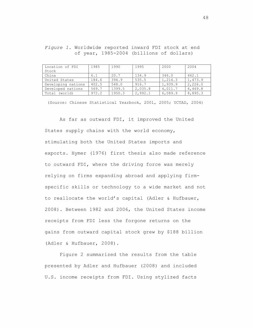
Figure 1. Worldwide reported inward FDI stock at end of year, 1985-2004 (billions of dollars)

Location of FDI Stock

1985 1990 1995 2000 2004

China 6.1 20.7 134.9 346.0 462.1 United States 184.6 394.9 535.5 1,214.3 1,473.9 Developing nations 402.5 548.0 916.7 1,939.9 2,226.0 Developed nations 569.7 1399.5 2,035.8 4,011.7 6,469.8 Total (world) 972.2 1950.3 2,992.1 6,089.9 8,895.3 (Source: Chinese Statistical Yearbook, 2001, 2005; UCTAD, 2004)

As far as outward FDI, it improved the United

States supply chains with the world economy,

stimulating both the United States imports and

exports. Hymer (1976) first thesis also made reference

to outward FDI, where the driving force was merely

relying on firms expanding abroad and applying firm-

specific skills or technology to a wide market and not

to reallocate the world’s capital (Adler & Hufbauer,

2008). Between 1982 and 2006, the United States income

receipts from FDI less the forgone returns on the

gains from outward capital stock grew by $188 billion

(Adler & Hufbauer, 2008).

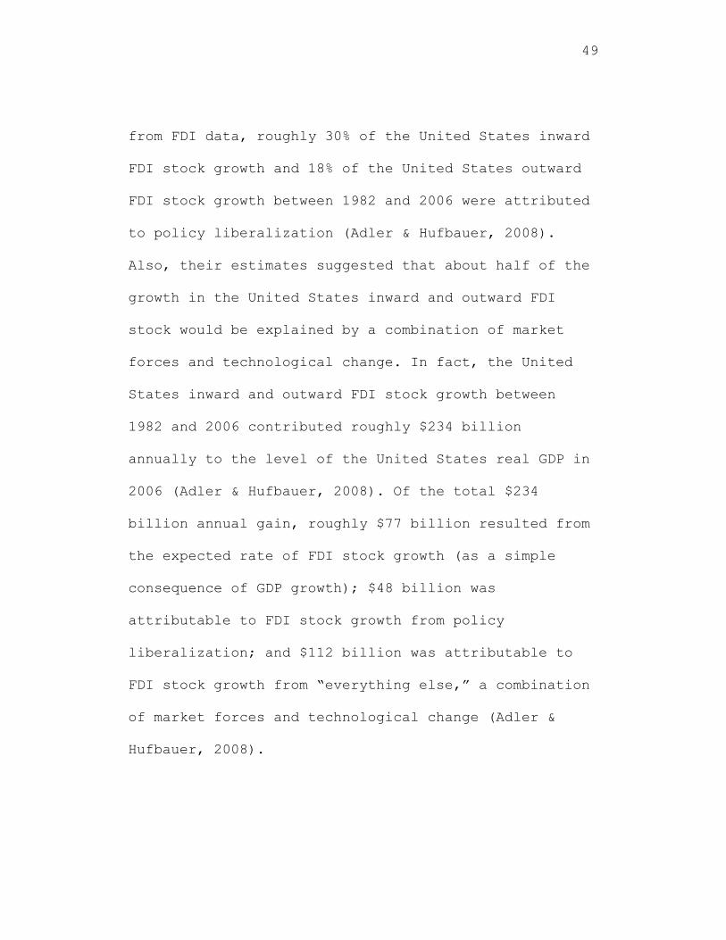
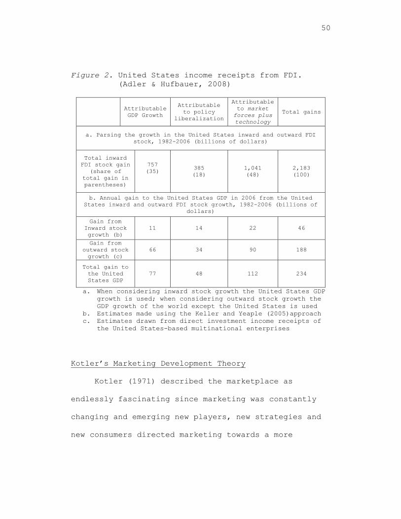
Figure 2 summarized the results from the table

presented by Adler and Hufbauer (2008) and included

U.S. income receipts from FDI. Using stylized facts

49

from FDI data, roughly 30% of the United States inward

FDI stock growth and 18% of the United States outward

FDI stock growth between 1982 and 2006 were attributed

to policy liberalization (Adler & Hufbauer, 2008).

Also, their estimates suggested that about half of the

growth in the United States inward and outward FDI

stock would be explained by a combination of market

forces and technological change. In fact, the United

States inward and outward FDI stock growth between

1982 and 2006 contributed roughly $234 billion

annually to the level of the United States real GDP in

2006 (Adler & Hufbauer, 2008). Of the total $234

billion annual gain, roughly $77 billion resulted from

the expected rate of FDI stock growth (as a simple

consequence of GDP growth); $48 billion was

attributable to FDI stock growth from policy

liberalization; and $112 billion was attributable to

FDI stock growth from “everything else,” a combination

of market forces and technological change (Adler &

Hufbauer, 2008).

50

Figure 2. United States income receipts from FDI. (Adler & Hufbauer, 2008)

Attributable GDP Growth

Attributable to policy

liberalization

Attributable to market forces plus technology

Total gains

a. Parsing the growth in the United States inward and outward FDI stock, 1982-2006 (billions of dollars)

Total inward FDI stock gain

(share of total gain in parentheses)

757 (35)

385 (18)

1,041 (48)

2,183 (100)

b. Annual gain to the United States GDP in 2006 from the United States inward and outward FDI stock growth, 1982-2006 (billions of

dollars)

Gain from Inward stock growth (b)

11 14 22 46

Gain from outward stock growth (c)

66 34 90 188

Total gain to the United States GDP

77 48 112 234

a. When considering inward stock growth the United States GDP growth is used; when considering outward stock growth the GDP growth of the world except the United States is used

b. Estimates made using the Keller and Yeaple (2005)approach c. Estimates drawn from direct investment income receipts of

the United States-based multinational enterprises

Kotler’s Marketing Development Theory

Kotler (1971) described the marketplace as

endlessly fascinating since marketing was constantly

changing and emerging new players, new strategies and

new consumers directed marketing towards a more

51

scientific approach through the use of modeling

concepts. The modeling concept was optimized with an

overall marketing optimization where all marketing

instruments were in need of a comprehensive marketing

system (Kotler, 1971, p. 667). In the area of

international FDI, for any new business launched,

whether an emerging technology or a mature business,

business planners must deal with at least five issues:

(1) what was the total demand, (2) what price would

the market bear, (3) would costs be controlled so that

the product would be built and sold at a profit, (4)

was the market ready for the product, (5) what were

the capabilities and intentions of competitors (Bers,

Lynn, & Spurling, 1997, p. 2).

Kotler (1997) further expanded marketing

techniques as trend analysis, substitution analysis,

and chain ratio analysis that would be applied to

estimate demand from prior history and industry

trends. In a mature market, new products had markets

for which dimensions would be determined; either the

product would displace existing competitors within

52

established market, or the product would be reasonably

close substitute for other established products (Bers,

Lynn, & Spurling, 1997, p. 2).

Kotler’s Buyers Behavior School of Thought

Kotler (1967) also referred to the evaluation of

the managerial school of thoughts through his buyer’s

behavior theory. He identified the key policy issues

of marketing practices and provided adequate

definitions to fundamental concepts such as the

product life cycle, the marketing mix, and market

segmentation (Sheth, Gardner & Garrett 1988, p. 105).

Through the buyer behavior theory, Kotler (1967)

sharply contrasted the production, selling, and

customer-oriented marketing philosophies with a strong

advocacy toward the latter orientation in marketing

practices. The buyer behavior school focused on

customers in the market place and in addition to the

demographic information on how many and who were the

customers. The buyer behavior school of marketing

attempted to address the question of why customers

53

behaved, the way they did in the marketplace (Sheth,

Gardner & Garrett 1988, p. 110). Such popularity of

the buyer behavior school indicated an analysis

suggesting two major reasons for the evaluation and

rapid popularity of the behavior school: (1) the

emergence of the marketing concept; and (2) the

established body of knowledge in behavioral science

(Sheth, Gardner & Garrett 1988, P. 111) (Figure 3). A

major area of research in buyer behavior focused on

social and public services such as population control,

education, health care, transportation, and nutrition

when utilized through FDI (Sheth & Wright, 1974). This

was also a direct result of the emerging interest in

applying marketing practice and concepts to nonprofit

organizations (Kotler, 1975) (Figure 3).

54

Figure 3. Evaluation of the Buyer Behavior School (Sheth, Gardner, & Garrett, 1988, p. 126)

Criterion

Rationale Score

Structure

Several specific constructs that are well defined and properly integrated.

8

Specification

Theories provide specific hypotheses that delimit their scope.

8

Testability

Problems with several midrange theories. 6

Empirical Support

Much Empirical research, but often-

conflicting results.

8

Richness

Produced comprehensive theories and highly generalizable midrange theories.

9

Simplicity

Mixed reviews

8

Total

47

The Activist School of Thoughts Theory

The Activist School of Thoughts was similar to

the buyer behavior theory since it took the

perspective of the consumer in the marketplace rather

than the marketer (Sheth, Gardner, & Garrett 1988).

Kotler (1972b) believed that the practice of the

marketing concept with its costumer orientation was

necessary to mesh the actions of business with the

interests of consumers (Sheth, Gardner & Garrett 1988,

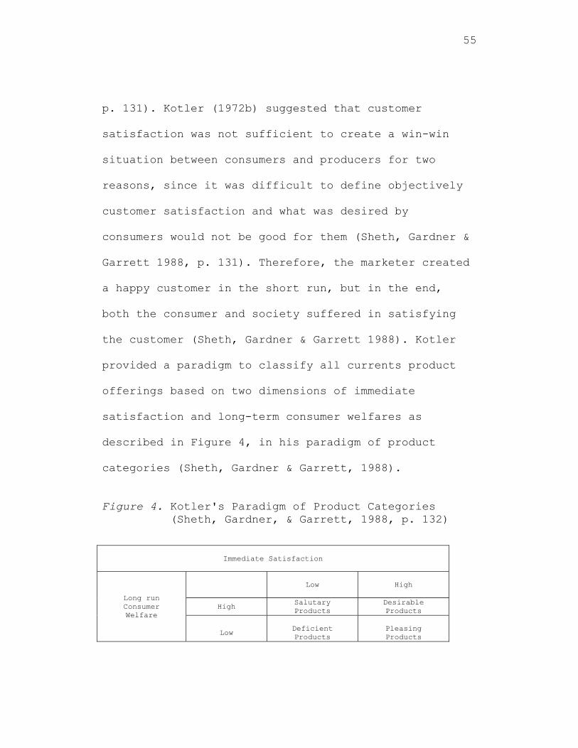
55

p. 131). Kotler (1972b) suggested that customer

satisfaction was not sufficient to create a win-win

situation between consumers and producers for two

reasons, since it was difficult to define objectively

customer satisfaction and what was desired by

consumers would not be good for them (Sheth, Gardner &

Garrett 1988, p. 131). Therefore, the marketer created

a happy customer in the short run, but in the end,

both the consumer and society suffered in satisfying

the customer (Sheth, Gardner & Garrett 1988). Kotler

provided a paradigm to classify all currents product

offerings based on two dimensions of immediate

satisfaction and long-term consumer welfares as

described in Figure 4, in his paradigm of product

categories (Sheth, Gardner & Garrett, 1988).

Figure 4. Kotler's Paradigm of Product Categories (Sheth, Gardner, & Garrett, 1988, p. 132)

Immediate Satisfaction

Long run Consumer Welfare

Low

High

High Salutary Products

Desirable Products

Low

Deficient Products

Pleasing Products

56

Kotler’s (1972b) fourfold classification of products

(see Figure 4), based on the two criteria of long-run

consumer welfare and immediate customer satisfaction

had considerable merit, suggesting that long run

consumer welfare measured marketing effectiveness,

whereas immediate customer satisfaction measured

marketing efficiency (Sheth, Gardner & Garrett 1988,

p. 132). In the process of FDI, an industry with many

desirable products was both effective, efficient, and

balanced the interests of the company and the public

(Sheth, Gardner & Garrett 1988, p. 133). On the other

hand, an industry full of pleasing products would be

very efficient or profitable, but would not be

effective from society’s viewpoint; therefore, it

would require social regulation (Sheth, Gardner &

Garrett 1988, p. 133).

Kotler (1986b) proposed a broadened view of

marketing, explicitly focusing on problems associated

with emerging blocked or protected markets (markets

characterized by high entry barriers through FDI).

Kotler suggested that marketing was increasingly

57

becoming a political exercise, by companies operating

in certain markets to master the art of supplying

benefits to parties other than target consumers

(Sheth, Gardner & Garrett 1988, p. 144). The need

extended beyond the requirements to serve and satisfy

normal intermediaries like agents, distributors and

agents (Sheth, Gardner & Garrett 1988, p. 144). Kotler

argued that, faced with blocked or protected markets,

marketers must engage in “Megamarketing, in which the

concept of power and public relations were given

emphasis, in addition to the four Ps of marketing

strategy, product, price, place, and promotion”

(Sheth, Gardner & Garrett 1988, p. 144).

In the area of pricing, Kotler (1997) related to

a useful tool for guiding value pricing was the price-

value grid, which helped firms when implementing FDI

to determine the efficacy of their value pricing, as

shown in Figure 5. (Weinstein, Johnson, & William,

1999, p. 93).

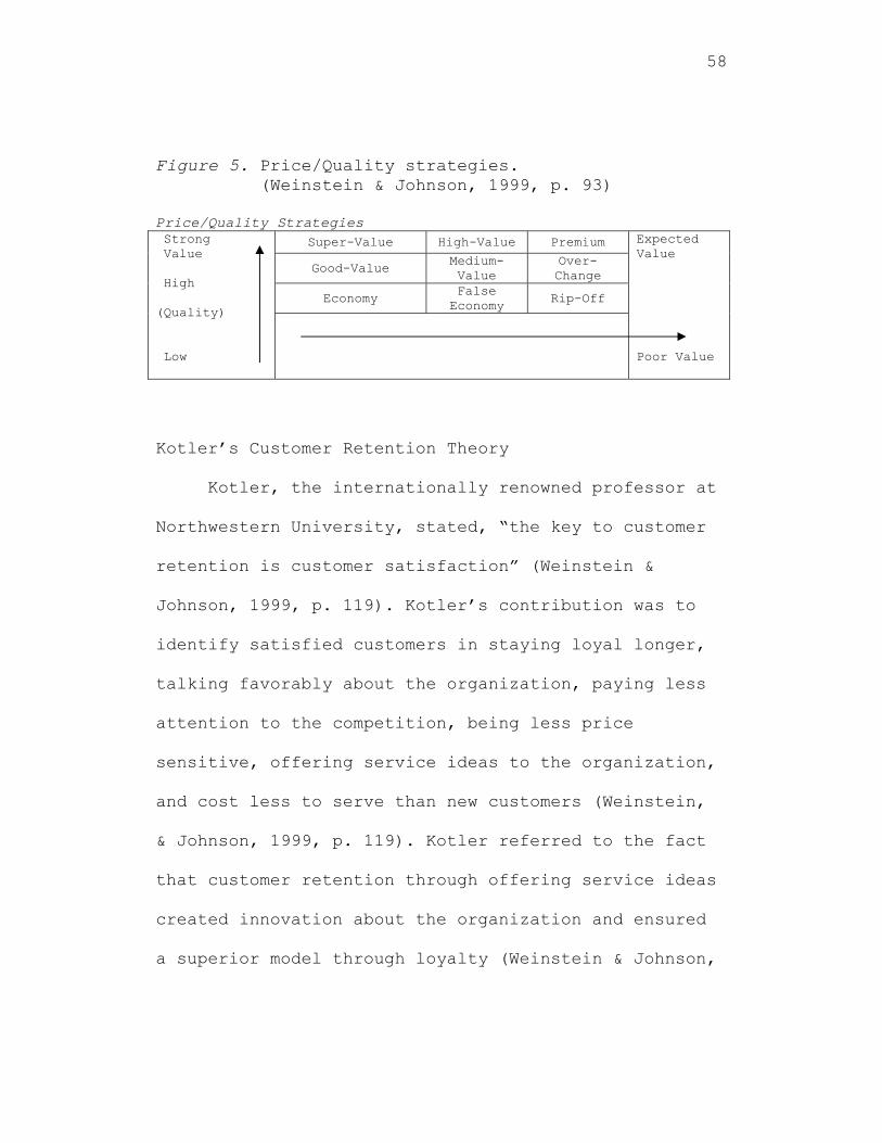
58

Figure 5. Price/Quality strategies. (Weinstein & Johnson, 1999, p. 93) Price/Quality Strategies Strong Value High (Quality) Low

Super-Value High-Value Premium Expected Value Poor Value

Good-Value Medium-Value

Over-Change

Economy False Economy

Rip-Off

Kotler’s Customer Retention Theory

Kotler, the internationally renowned professor at

Northwestern University, stated, “the key to customer

retention is customer satisfaction” (Weinstein &

Johnson, 1999, p. 119). Kotler’s contribution was to

identify satisfied customers in staying loyal longer,

talking favorably about the organization, paying less

attention to the competition, being less price

sensitive, offering service ideas to the organization,

and cost less to serve than new customers (Weinstein,

& Johnson, 1999, p. 119). Kotler referred to the fact

that customer retention through offering service ideas

created innovation about the organization and ensured

a superior model through loyalty (Weinstein & Johnson,

59

1999, p. 119). Loyalty further expanded in the core

elements that created value in an organization where

Kotler’s theory played a vital role in the founding

principle of customer retention (Weinstein & Johnson,

1999, p. 119). Customer value was built through the

proper mix of quality, service, price (QSP), image,

innovation, and intangible (the 3I’s), those elements

that attracted customer to the organization

(Weinstein, & Johnson, 1999, p. 120). The traditional

marketing paradigm of the 4P’s of marketing, expanded

by Kotler’s Megamarketing created short-term

perspectives. He also stated that companies would move

from a short-term transaction orientation to long-term

relationship-building goals, specificaly when

expanding abroad from the host country (Weinstein, &

Johnson, 1999, p. 132). The relationship of long-term

building goals was the objective in which Kotler

examined that would create a more profound, solid

market foundation and a permanent principle where

retention would be diluted in creating and keeping

customers (Weinstein & Johnson, 1999). By creating

60

more profound solid customer retention, a loyal

customer base would represent a fundamental

transformation that would enhance a traditional market

for business success away from the host country

(Weinstein & Johnson, 1999).

Competitive Strategic Decision-making

Through competitive strategy, a firm’s central

goal would create long-term superior return on

investment (Porter, 1996). A strategy was situation

specific, consistent of external and internal factors

and distinctive competence as the central idea to the

company, specifically as they expand their operations

to foreign countries (Porter, 1996).

Porter, an economics professor at Harvard

Business School, is a leading advocate in the

strategic decision making process and a contributor in

the theoretical concept of strategy as it pertained to

competitive, market changes and superior performance

of a firm (Porter, 1996). In strategy, managers had

been learning to play by a new set of rules, where

61

companies were flexible to respond rapidly to

competitive and market changes as they transfer their

operations through FDI (Porter, 1996, p. 62).

Therefore, through strategy, it would be able to

provide a variety of management decisions, resulting

from benchmarking continuously, outsourcing

aggressively to gain efficiency and positioning of a

firm (Porter, 1996).

Strategy was broadly expanded from the

battlefield of wars and became a more significant part

of the management process after World War II (Pearce &

Robinson, 2003). Through strategy, a company’s game

plan was explored and broadly understood as a

framework for managerial decision. A strategy

reflected a company’s awareness of how, when, and

where it would compete; against whom it would compete;

and for what purposes it would compete (Pearce &

Robinson, 2003, p. 4). Similarly, strategic management

was defined as a set of decisions and actions,

resulting in the formulation and implementation of

plans designed to achieve a company’s objectives

62

(Pearce & Robinson, 2003, p. 3). Similarly, strategic

decision making had social responsibilities, ranging

from mission statements expressed in terms of how the

company intended to contribute to the society that

sustained it to corporate performance (Pearce &

Robinson, 2003, p. 15).

Porter’s Competitive Advantage Theory

Porter’s Competitive Advantage referred to the

sources surrounding the prominent sources, consisting

of cost leadership, differentiation, market focus and

speed (Porter, 2001). Porter (2001) illustrated that

the average profitability under pressure in many

industries was influenced by the Internet. Therefore,

it was imperative individual companies achieved a

sustainable competitive advantage by operating at a

lower cost, allowing a premium price, or a combination

of both (Porter, 2001). Porter (2001) further added

that cost and price advantages would be achieved in

two ways. One was operational effectiveness or doing

the same things competitors do, but doing them better.

63

Second was the ability to improving operational

effectiveness. Companies increased sustainable

advantages if they were able to achieve and sustain

higher levels of operational effectiveness than

competitors (Porter, 2001, p. 71). Such sustainable

advantage would be identified once companies extend

their operations in a foreign country. Porter (2001)

further added that rivals tended to copy best

practices in competition quickly, eventually leading

to competitive convergence with companies doing the

same things in the same way, where customers decided

on price and undermining industry profitability. A

company can outperform rivals only if it established a

difference that would be preserved by delivering a

greater value to customers or would create comparable

value at a lower cost, or do both (Porter, 1996, p.

62). The arithmetic of superior profitability followed

by delivering a greater value by allowing a company to

charge higher average unit prices and increasing

efficiency resulting in lower average unit costs

(Porter, 1996, p. 62).

64

By contrast, operational effectiveness referred

to any number of practices that allowed a company to

better utilize its inputs by reducing defects in

products or developing better products faster (Porter,

1996, p. 62). Differences in operational effectiveness

were at the heart of the Japanese challenge to Western

companies in the 1980s, in which the Japanese were far

ahead in operational effectiveness allowing them to

lower cost and providing a superior quality at the

same time (Porter, 1996, p. 62). This operational

effectiveness was also attributed to lean production

displaying an overall substantial improvement in

manufacturing productivity and asset utilization, as

well as TQM (Total Quality Management) and

benchmarking maximizing efficiency, whereby improving

customer satisfaction and best practices (Porter,

1996, p. 63). The result of the competitors by

operational effectiveness would quickly imitate

management techniques, new technologies, input

improvements, and superior ways of meeting customer’s

needs (Porter, 1996, p. 63).

65

The second way was achieving advantage through

strategic positioning, or doing things differently

from competitors in a way that delivered a unique type

of value to customers (Porter 2001, p. 70). By

applying strategic positioning once FDI is considered,

the only way to generate higher levels of economic

value was to gain a cost advantage or price premium by

competing in a distinctive way, which would lead to

being ahead of its competition (Porter, 2001, p. 72).

Porter (2001) inferred that without distinctive

strategic direction, speed and flexibility would lead

nowhere, either no unique competitive advantages would

be created, or improvements would be generic and would

not be sustained. Porter (2001) rationale was that

strategy was a matter of discipline, requiring and

viewing profitability as the central focus rather than

relying on a company’s overall growth. Porter (2001)

proactive role was the company’s direction toward

making tough decisions during time of upheaval, for

example operating in foreign countries, while pressing

66

on issues of the company focus on distinct positioning

in the best practice to remain competitive.

Porter (1980) provided a conceptual view, such as

new product introductions and price decreases that

would have potentially negative impact on

profitability of other players in the industry, and

therefore, countermoves would be expected. By

contrast, cooperative or non-threatening moves did not

trigger competitive responses. Cooperative moves had

the property that they did not interfere with the

objectives of the rival competitor (Kuester, Homburg &

Robertson, 1999, p. 91). Price increases were

generally designed as cooperative moves. The initiator

anticipated that other competitors would follow

(Kuester et al., 1999, p. 91). A firm would respond to

competitive actions, which would add sustainability or

competitive advantage and would determine the

company’s organizational performance reacting strongly

to the new product, which would jeopardized once it

was introduced to the consumer (Kuester et al., 1999,

p. 91).

67

Porter’s Three Generic Strategies

Porter’s Product Differentiation

According to Porter (1980), the first generic

firm strategies was differentiation, which involved a

firm creating higher value than its competitors based

on various elements, including brand image, product

positioning, customer service and differentiated

components in a product, etc. Porter (1980) further

explained that a firm used differentiation by citing

to include design or brand image, technology,

features, customer service, and dealer network.

According to Pearce and Robinson (2003), the

differentiation of products was real or perceived,

often intensified by competition among existing firms.

Firms operating internationally were able to compete

for differentiation which was advantageous based on

certain design principles or a change of technology

(Pearce & Robinson, 2003). However, successful

differentiation posed a competitive disadvantage for

firms that attempted to enter an industry (Pearce,

Robinson, 2003, p. 79).

68

Perceived differentiation was further expanded on

firms attempting to sell their product by educating

the consumer that their product differed significantly

from the competition (Pearce & Robinson, 2003). The

significant difference would create a symbolic value

or a significant distinctiveness that would create an

attraction toward certain customers (Pearce &

Robinson, 2003). Porter’s (1980) differentiation

theory was compared to Miles and Snow’s (1978)

prospectors theory which stated that firms continually

searching for new markets, for example operating

through FDI ventures, which in certain cases, was

favorable, but also less efficient due to the markets

inability to allowed promoting from within an

organization.

Porter’s Overall Cost Leadership

Porter (1980) stated in his second generic

strategy that a firm, using overall cost leadership

strategy, seeked to produce its product at the lowest

cost in an industry. Striving for low cost leadership

69

would achieve certain capabilities to include having

secured suppliers of scarce raw materials, being in a

dominant market share position, or having a high

degree of capitalization (Pearce, Robinson, 2003, p.

160). Such specialization would be attributed when

enduring FDI practices. A low cost leader was able to

enjoy cost reduction, which would have a direct effect

in improving overall sustainability in maximizing

economies of scales and cost-cutting techniques in

technologies and reduction in overhead expenses

(Pearce & Robinson, 2003, p. 160). The cost leader was

also able to apply cost advantage to charge lower

prices or to enjoy higher profit margins. Therefore, a

firm such as one in an FDI venture would effectively

defend itself in price wars would attack competitors

on price to gain market share, or, if already dominant

in the industry, would simply benefit from exceptional

returns (Pearce, Robinson, 2003, p. 160).

70

Porter’s Focus Strategy

According to Porter (1980), third generic

strategy a firm would utilize focus strategy for

maximizing profitability. By conducting a more

profound focus of an industry, Porter (1980), added

that a firm was able to concentrate on certain segment

areas of strategic target market more effectively than

a competitors’ holistic approach that was competing

broadly. A firm pursuing a focus strategy was willing

to service isolated geographic areas to satisfy the

needs of customers with special financing, inventory,

or servicing problems; or to tailor the product to a

unique demand of the small to medium sized customer

(Pearce, Robinson, 2003, p. 161). The focusing firm

was able to profit from their willingness to serve

otherwise ignored or underappreciated customer segment

(Pearce, Robinson, 2003, p. 161). A prime example of

focus strategy was firms conducting FDI through MNCs

willingness to serve isolated rural areas away from

urban locations, served by traditional markets. This

allowed these firms utilizing a focus approach to have

71

greater than average industry returns (Pearce &

Robinson, 2003).

FDI in Cuba’s Product and Service Sector

Cuba’s Economic Infrastructure prior to 1959

Cuba’s economy and distribution of goods was

similarly well developed in the 1950s. Of the total

value of wholesale trade and services in 1955,

imported products accounted for 55 percent and

domestic products for 45 percent (Institute for Cuban

Studies, 2001, p. 1). Local markets in both the

product and service sectors had a variety of wholesale

and retail trades that was carried simultaneously,

while there was no price list published and no indices

existed to give farmers a reliable estimate of the

worth of their products (Institute for Cuban Studies,

2001, p. 1). At that time, merchants had an

opportunity to exploit both farmer and consumer since

the goods were not subject to any grading method

(Institute for Cuban Studies, 2001, p. 1). However,

72

farmers were able to sell some products to nearby

towns and in remote areas. These farmers resorted to

bartering and cash exchange developed (Institute for

Cuban Studies, 2001). The cash exchange between

farmers and nearby towns led the way for a supply

chain to develop, between retailers and wholesalers,

from towns to major cities including the capital of

Havana that was able to profit from these exchanges.

Before 1959, retail prices were assigned

inconsistently with mark-ups on the United States

items ranging frequently between 20 percent and 200

percent above the United States retail price. Prices

often varied according to the avenues of trades from

manufacturer to consumer. Some manufactures sold

directly to small retail outfits, while others

preferred bulk sales to wholesalers (Institute for

Cuban Studies, 2001).

Cuba was a relatively advanced country in 1958,

certainly by Latin American standards and, in some

areas, by world standards (Institute for Cuban

Studies, 2002, p. 1). The data appeared to indicate

73

that Cuba had maintained high levels of development in

health and education, but at an extraordinary cost to

the overall welfare of the Cuban people, to include

access to basics levels of food, electricity and

access to consumer goods availability which increased

in recent decades in other Latin American countries

(Institute for Cuban Studies, 2002, p. 1). Cuba had an

excellent educational system and impressive literacy

rates in the 1950s, which ranked the 13th lowest in the

world (Institute for Cuban Studies, 2002, p. 1).

As far as the capita food consumption, Cuba

ranked third in Latin America in per capita food

consumption, today it ranks last (Institute for Cuban

Studies, 2002, p. 1). The 1960 UN statistical yearbook

ranked pre-revolutionary Cuba third out of 11 Latin

American countries based on per capita daily caloric

consumption. In 2002, Cuba ranked last (Institute for

Cuban Studies, 2002, p. 2). The number of telephone

lines in Cuba once ranked first in Latin America and

fifth in the world in television sets per capita,

whereas in 2002, it barely ranked fourth in Latin

74

America and was well back in ranks globally (Institute

for Cuban Studies, 2002, p. 1). In 1957, Cuba had more

television stations (23) than any other country in

Latin America, easily outdistancing larger countries

such as Mexico (12 television stations) and Venezuela

(10 television stations) (Institute for Cuban Studies,

2002, p. 5).

During the late 1950s, Cuba ranked second only to

Uruguay in Latin America in terms of radios per

capita, with 169 radios per 1,000 people (Institute

for Cuban Studies, 2002, p. 4). Cuba also ranked

eighth in the world in number of radio stations (160),

ahead of such countries as Austria (83 radio

stations), United Kingdom (62), and France (50),

according to UN statistical yearbook (Institute for

Cuban Studies, 2002, p. 5). In addition, Cuba’s rice

production has fallen since 1958, when it ranked

fourth in the region in production of this staple

(Institute for Cuban Studies, 2002, p. 4). Cuba’s

export in 1958 far exceeded those of Chile and

Colombia, countries that have since exceeded Cuba’s

75

export due to Cuba’s inability to diversify their

export to other countries in the hemisphere (Institute

for Cuban Studies, 2002). As of 1958, the value of the

United States FDI (foreign direct investment) in Cuba

was $861 million, and adjusting for inflation that

foreign investment number amounts to more than 4.3

billion United States dollars in today’s currency

(Institute for Cuban Studies, 2002, p. 5).

In the case of sugar production, the United

States’ investors were not focused on the sugar

industry in the beginning of 1935, and began selling

their Cuban sugar holdings to Cuban firms (Institute

for Cuban Studies, 2002, p. 4). By 1958, the United

States’ firms owned fewer than 40 of the 161 Cuba’s

sugar mills since the United States’ firms were

investing in a range of other venture, especially in

infrastructure development (Institute for Cuban

Studies, 2002, p. 5). Advances were made in the sugar

mills where the use of machinery and steam replaced

animals in the production and transportation of sugar

(Institute for Cuban Studies, 2002, P. 5). Cuba’s

76

economy was healthy in 1958, with gold as a foreign

exchange reserve, which was the preferred measure at

that time of a healthy balance of payments. It had a

total of $387 million in 1958 (Institute for Cuban

Studies, 2002, p. 5). In 1958, Cuba’s reserves ranked

third in Latin American behind Venezuela and Brazil,

which was impressive by Latin America standards since

the population in the island was fewer than 7 million

people (Institute for Cuban Studies, 2002, p. 5).

Cuba’s Economic Infrastructure, 1959 TO 1989

On January 7, 1959, the United States recognized

that the government of Fidel Castro as the ruling

party of Cuba. Cuba’s government changed from a

dictatorship under Fulgencio Batista under a

democratic economic system to a totalitarian communist

centrally planned system under Fidel Castro (Institute

for Cuban Studies, 2002). After Cuba signed a trade

agreement with the former Soviet Union in 1960 for the

purpose of Cuba bartering sugar for crude oil from the

Soviet Union, the relationship between Cuba and the

77

United States declined during the time period of the

Cold War, leading to a total trade embargo by the

United States on exports to Cuba (except medicine and

food) (Institute for Cuban Studies, 2002). By 1961,

Fidel Castro acknowledged the Marxist-Leninist

affiliation, identifying Cuba’s revolution as

socialist, anti-imperialist and implementing a

centrally planned system of government. The centrally

planned system of government in Cuba seized private

companies and the control of the public sector was

solely governed by a communist regime (Institute for

Cuban Studies, 2002). Soviet assistance and subsidies

kept the Cuban economy afloat from the 1960s until the

end of the Soviet Union in 1991 (the United States

Department of State, 2003, p. 1).

Since the 1960s, the quality of life in Cuba had

deteriorated with a depletion of the middle class

exiting the island and migrating to the United States.

The centrally planned system eliminated the private

sector and the public sector was controlled by the

Castro government, dictating the product/services’

78

supply chain (United States Department of State,

2003). Cuba per capita consumption of cereals, tubers,

and meat are today all below 1950s levels (Institute

for Cuban Studies, 2002, p. 1). The number of

automobiles in Cuba had fallen since the 1950s, as

well as telephone lines in Cuba had been virtually

frozen at 1950s levels (Institute for Cuban Studies,

2002, p. 1). The Castro government also shut down what

was a remarkably vibrant media sector in the 1950s. At

that time, Cuba, a small country, had 58 daily

newspapers of differing political views and current

information on business information. Cuba ranked

eighth in the world in number of radio stations

(Institute for Cuban Studies, 2002, p. 1).

Cuba’s government after 1959, appraised as having

one of the most advanced health care system, even

though the analysis ignored the fact that the

revolutionary government inherited an already advanced

health care system when it took power in 1959 from the

previous government of Fulgencio Batista (Institute

for Cuban Studies, 2002, p. 2).

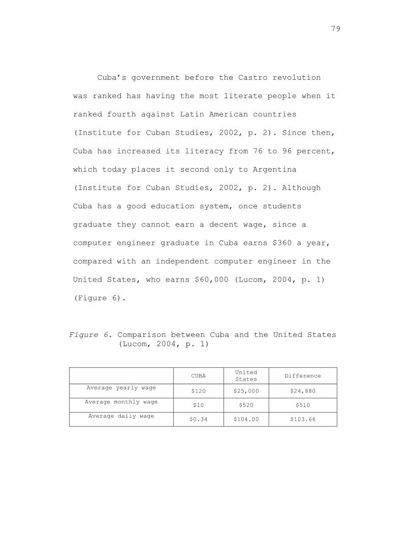
79

Cuba’s government before the Castro revolution

was ranked has having the most literate people when it

ranked fourth against Latin American countries

(Institute for Cuban Studies, 2002, p. 2). Since then,

Cuba has increased its literacy from 76 to 96 percent,

which today places it second only to Argentina

(Institute for Cuban Studies, 2002, p. 2). Although

Cuba has a good education system, once students

graduate they cannot earn a decent wage, since a

computer engineer graduate in Cuba earns $360 a year,

compared with an independent computer engineer in the

United States, who earns $60,000 (Lucom, 2004, p. 1)

(Figure 6).

Figure 6. Comparison between Cuba and the United States (Lucom, 2004, p. 1)

CUBA United States

Difference

Average yearly wage

$120 $25,000 $24,880

Average monthly wage $10 $520 $510

Average daily wage

$0.34 $104.00 $103.66

80

From 1963 through 1977, an examination showed

that the Cuban Economy indicated a period of rise and

decline with the country’s Gross Domestic Product

(GDP) (Mesa-Lago, 1979). The Cuban economy went

through a decline starting from 1962-63, which was the

lowest indicator in GDP as a basis of reform that the

revolution undertook as a centrally planned system

went into effect with a stabilization process (Mesa-

Lago, 1979, p. 98). From 1963-1965, a rise in GDP

occurred on a small fraction since annual GDP absolute

showed 3.8 percent per 100 and 1.2 percent per 100

capita (Mesa-Lago, 1979, p. 98) (Figure 7). From 1967

through 1977, there were indicators of GDP decline due

to an inflation which affected the country’s ability

of economic prosperity; even though, 1966 through

1970, the country’s economy deteriorated severely with

GDP declining at 0.4 percent per 100 and -1.3 percent

per 100 capita (Mesa-Lago, 1979, p. 98). By 1971

through 1977, Cuba’s economy began a recuperation

process due to more profound economic measures,

specifically from 1971-72, particularly during the

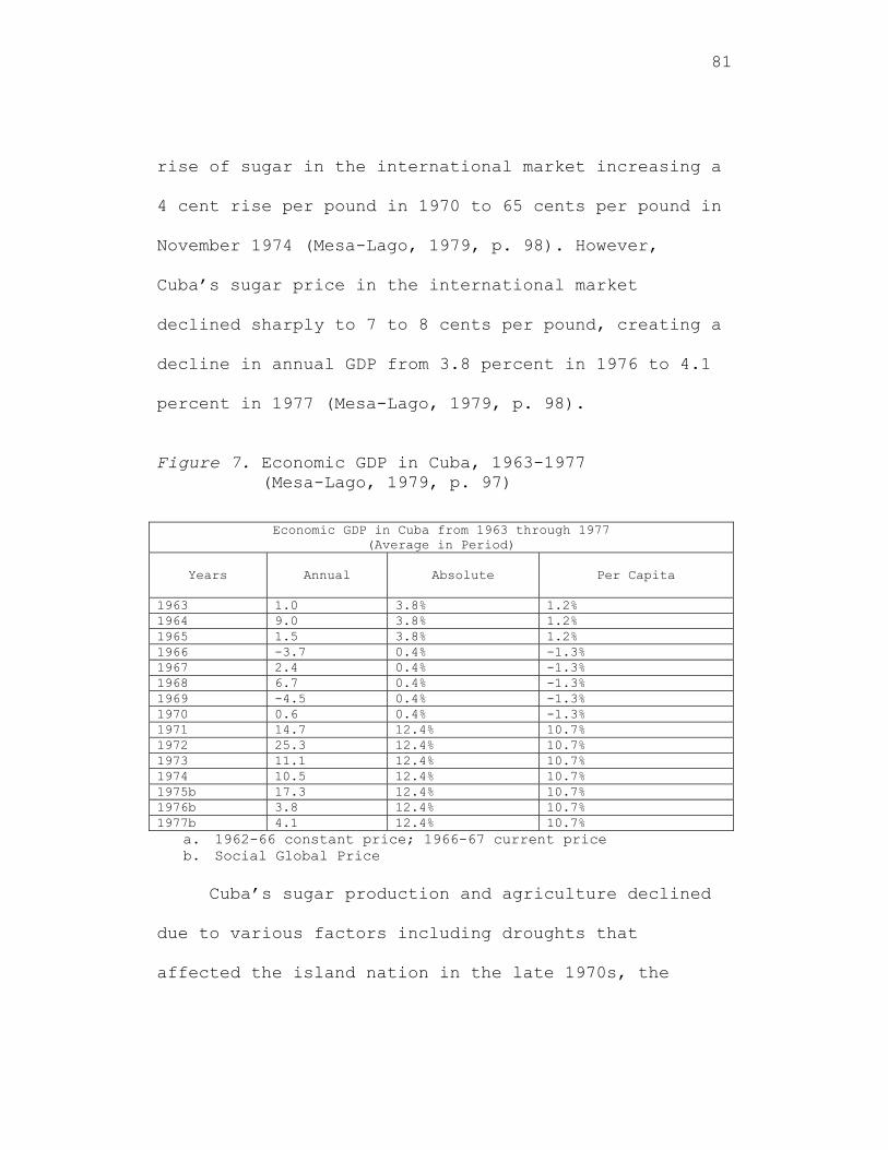
81

rise of sugar in the international market increasing a

4 cent rise per pound in 1970 to 65 cents per pound in

November 1974 (Mesa-Lago, 1979, p. 98). However,

Cuba’s sugar price in the international market

declined sharply to 7 to 8 cents per pound, creating a

decline in annual GDP from 3.8 percent in 1976 to 4.1

percent in 1977 (Mesa-Lago, 1979, p. 98).

Figure 7. Economic GDP in Cuba, 1963-1977

(Mesa-Lago, 1979, p. 97)

Economic GDP in Cuba from 1963 through 1977 (Average in Period)

Years

Annual Absolute Per Capita

1963 1.0 3.8% 1.2% 1964 9.0 3.8% 1.2% 1965 1.5 3.8% 1.2% 1966 -3.7 0.4% -1.3% 1967 2.4 0.4% -1.3% 1968 6.7 0.4% -1.3% 1969 -4.5 0.4% -1.3% 1970 0.6 0.4% -1.3% 1971 14.7 12.4% 10.7% 1972 25.3 12.4% 10.7% 1973 11.1 12.4% 10.7% 1974 10.5 12.4% 10.7% 1975b 17.3 12.4% 10.7% 1976b 3.8 12.4% 10.7% 1977b 4.1 12.4% 10.7%

a. 1962-66 constant price; 1966-67 current price b. Social Global Price

Cuba’s sugar production and agriculture declined

due to various factors including droughts that

affected the island nation in the late 1970s, the

82

decline in sugar price in the world’s market, the

delay in modernizing the country’s sugar mills and

agricultural mills by the assistance of the Soviet

Union, which affected Cuba’s economic infrastructure

by start of the 1980s’ (Mesa-Lago, 1979, p. 102). By

1982, Cuba was unable to repay principal on external

debts estimated at 10.5 billion to 11 billion dollars,

including hard currency debts of about 3 billion US

dollars (Wall Street Journal, 1982, p. 1). Cuba was

also subject to being unable to repay their external

debts but also to repay their debts to international

banks, which placed the country in a deteriorating

financial crisis throughout the 1980s (Wall Street

Journal, 1982, p. 1). “By 1989, the collapse of

communism in Eastern Europe, followed by the former

Soviet Union, brought the Cuban economy to a further

decline at least 35-40 percent from 1990 through 1993,

when aid to Cuba was cut off by the former Soviet

Union and other Eastern Bloc countries” (Font, 1996,

p. 1).

83

Cuban Democracy Act of 1992

By 1991, the Cuban economy contracted even

further by 25 percent. It also contracted by 10

percent per year for three consecutive years, forcing

the question of reform that led to the Cuban Democracy

Act of 1992 with the Torriceli Act and The Helms-

Burton Act that followed in 1994 (Font, 1996, p. 3).

As the crisis began in the early 1990s and deepened in

1993, internal reforms were adapted by the Cuban

government in order for Cubans to hold dollars and use

them in commercial transactions throughout the island

since the onset of the revolution in 1959 (Font, 1996,

p. 5). These internal reforms led the way to a wide

differential between the official exchange rate and

the black-market rate (still 25-30 pesos to one U.S.

dollar), but as high as 120 to 1 in 1994 (Font, 1996,

p. 5). As a result, this measure encouraged the inflow

of dollars, which led the way for the Cuban government

in setting up dollar stores and currency exchange

office to capture the bulk of incoming hard currency

(Font, 1996, p. 5). As the number of goods and

84

services transacted in dollars increased, a growing

number of Cubans felt the need to obtain and use them,

thus fueling the emergent markets in dollars and

creating a private sector root within the central

planned economic system that existed in Cuba (Font,

1996, p. 5).

The Cuban Democracy Act (CDA), introduced by the

United States Representative Robert Toricelli in 1992,

forbade foreign subsidiaries of the United States

companies from dealing with Cuba. However, encouraged

through legislation, the assistance of the Cuban

people by reducing certain sanctions imposed by the

United States embargo in 1960 and allowing for

response to positive development in Cuba’s economy,

specifically telecommunications (Inside the United

States Trade, 1992, p. 8). By 1994, Cuba began

consolidations, particularly on fiscal adjustments

calling for higher taxes and lower expenditures as

well as monetary policies to reduce pressure on the

peso and accommodate the new economic sectors (Font,

1996, p. 7). The budget deficit was also reduced and

85

the value of the dollar in the open market was brought

to pre-1993 black market levels, allowing for food

production and distribution with the decentralization

of agriculture and the farmer’s market. This process

further pushed prices down, proclaiming small positive

growth rates for 1994 and 1995, at 0.7 percent and 2.5

percent, and even a higher rate of 5 percent for 1996

(Font, 1996, p. 7).

Cuba was also able to expand in the international

market with Canada and Mexico where trades were common

with these countries (Font, 1996, p. 10). Moreover,

the relationship with Mexico expanded even further

with 200 companies having commercialized relations

with Cuba. In addition, Canada became one of Cuba’s

leading economic partners in the 1990s. Cuba also

allowed 20 to 30 Canadian companies to invest

approximately 150 million U.S. dollars, largely in

mining and tourism that led the way in the development

of new hotels and resorts for Canadian tourist

visiting the island nation (Font, 1996, p. 12).

Canada’s stake even expanded with Cuba in the

86

production of nickel and cobalt mining in eastern Cuba

(Font, 1996, p. 12). The joint venture between Cuba

and the Canadian company Canada’s Sherritt, Inc,

invested about 165 million dollars to modernize the

Moa Bay Plant initially built in the late 1950s, by

the United States in order to produce 24,000 tons of

nickel and cobalt a year by 1999. An additional $175

million was invested to double production in the

following decades (Font, 1996, p. 12).

The Helm-Burton Law, known as the Cuban Liberty

and Democratic Solidarity Act, was an attempt to

tighten and broaden the United States embargo of Cuba

that emerged under the late Senator, Jesse Helms, and

the United States Representative, Dan Burton

(Vanderbush & Haney, 2002, p. 174). One of the clauses

in the Helm-Burton Law in Title IV was to deter

further economic activity in Cuba by foreign companies

and to induce divestment by companies currently doing

business on the island (the United States Congress

1996, p. 66). The primary targets of enforcement were

executives of the Canadian firm Sherritt International

87

and the Mexican firm Grupo Domos and the Italian

Company Stet International for doing business with

Cuba (Vanderbush & Haney, 2002, p. 177). Grupo Domos,

a partner in the Cuban telephone company relinquished

its stake due to a combination of the weak Cuban peso

and the threat posed by the Helm-Burton Law

(Vanderbush & Haney, 2002, p. 177). Stet, another

telecommunication company on the other hand, immunized

itself against Helm-Burton by agreeing to compensate

ITT (International Telephone & Telegraph) company for

their confiscated assets (Jonquieres, 1997, p. 4).

Sherritt International Corporation was later excluded

from the United States because of title IV, but the

clause in the Helms-Burton Law did make Canadian

executives who operated in Cuba liable to law suits in

United States courts and sanctions from the United

States government (Font, 1996, p. 13). For Cuba,

Canada was a very important and political partner.

Precisely how Canada chose to exercise this advantage

had considerable internal implications (Font, 1996, p.

13). The Helm-Burton Law did provide a further

88

modification for democratization of the island to

include the proposed sale of food by the United States

companies and American farms, as well as medicine to

the Cuban people (Vanderbush, Haney, 2002, p. 181).

For Cuba, the emerging of economic partners also

surfaced in the mid 1990s with the European Union,

building partnership with countries like Spain,

France, and the Netherlands (Font, 1996, p. 13). In

1994-95 and after, companies like Spain’s Tabacelera,

France’s Seita, and London’s Hunters & Frankau

received income credits of 40 million per year from

the European Union, allowing these companies to

purchase tobacco crops directly from Cuba (Font, 1996,

p. 13). Spanish entrepreneurs also invested $350

million in hotels and tourist facilities. However, by

1996, European Union’s suspended negotiations with the

Cuban government due to Cuba’s inability to conduct

economic and political reforms (Font, 1996, p. 13).

Latin America, like the European Union, has also been

involved in commercial and diplomatic relations with

Cuba, particularly in the travel and tourism but the

89

partnership did not create an economic integration in

the 1990s like Canada, Mexico and the European Union

(Font, 1996). The biggest obstacles from foreign firms

integrating in an economic partnership with Cuba by

the end of the decade of the 1990s was the Helm-Burton

Law, creating a chilling effect with enforcement being

imposed by the United States (Font, 1996, p. 15).

However, there are foreign firms that see the Helm-

Burton Law as an arbitrary and offensive imposition by

the United State government (Font, 1996, p. 15).

Cuba’s Economic Infrastructure, 1989 TO 2001

In June 2000, the United States’ Congress lifted

sanctions on sales of agriculture products and

medicine to Cuba (Calzon, 2002, p. 3). At the start of

the millennium, Cuba was financially bankrupt,

accumulating a vast amount of debt since 1986.

Castro’s Western creditors (including Canada, France

and Spain) have sought to recover some part of their

$10 billion dollars in loans to Cuba (Calzon, 2002, p.

3). In fact, the amount of loans accrued from years of

90

conducting business with Western nations like Canada,

Mexico and some of the European countries created debt

that had not been paid and had diminish Cuba’s ability

to acquire future credit (Calzon, 2002). Havana

refused to even repay Moscow’s larger loans from the

former Soviet Union, since they insisted the debt was

to the Soviet Union and not Russia, “a country that no

longer exists” (Calzon, 2002, p. 3).

American agribusiness believed there were huge

profits to be made by trading with Havana, since a

foreign policy consideration would not prevent trade

even if strengthening regimes like Libya, Iraq, and

Cuba would someday put lives of the United States’

servicemen at risk (Calzon, 2002, p. 3). Cuba trades

with the United States had been on a humanitarian

level (food and medicine) and on a cash basis only due

to Cuba’s inability to pay loans on credit, resulting

from Cuba’s past practice in defaulting on credit

purchased from foreign trade countries (Calzon, 2002,

p. 3).

Cuba’s financial decline was due to the following

91

1. Cuba’s economic woes continued to mount as a

result of being especially hard hit by the world

wide economics slow down and the fall-off in

international travel after the September 11

attacks (Calzon, 2002, p. 3).

2. Tourism, Cuba’s most important economic sector

had declined sharply. Hotel occupancy was down at

least 25 percent in Havana and 40 percent in

Varadero (Cuba’s most popular beach resort)

(Calzon, 2002, p. 3).

3. Cuba’s second largest source of foreign exchange,

expatriate remittances were down due to the

downturn in the United States (Calzon, 2002, p.

3).

4. Removal of Russian surveillance facilities cost

the Cuban economy $200 million dollars in Russian

rent (Calzon, 2002, p. 4).

5. Cuba’s former Vice President Carlos Lage had

cited “the hard blow by a fall in the world

prices for Cuba’s commodity exports such as sugar

and nickel” (Calzon, 2002, p. 4).

92

Recent and reliable good economic data about Cuba

are difficult to obtain, but during the year 2000,

France withheld a shipment of grain due to Castro’s

inability to pay for earlier transactions and canceled

$160 million dollars in new credits to Havana (Calzon,

2002, p. 4). Furthermore, in earlier 2001, Chile was

attempting to establish a payment plan for a $20

million debt for mackerel shipped the previous year

(Calzon, 2002, p. 4).

Another country, South Africa, according to The

Johannesburg Sunday Times was frustrated by Havana’s

failure to settle a $13 million dollar debt, and

Pretoria’s Trade and Industry Ministry refused to

approve credit guarantees to Cuba (Calzon, 2002, p.

4). Lastly, Thailand also refused to provide export

insurance, resulting in the cancellation of rice sales

to the island worth millions of dollars (Calzon, 2002,

p. 4).

According to a United States’ Commission Report,

rice exports to Cuba would be worth between $40

million and $59 million dollars, increasing the value

93

of the United States rice exports by 4 to 6 percent

(Calzon, 2002, p. 4). The problem with this analogy

was the United States exporters would be highly

competitive with current suppliers is that Castro’s

trade would be based on politics and not on economic

conditions. In turn, it could backfire since a

centralized system of government would favored the

government ability to acquire wealth by improvising a

share of more than 51 percent to Cuba’s ideological

allies like China and Vietnam and not favored any FDI

investment from the United States (Calzon, 2002, p.4).

This evidence had been noted in previous and recent

foreign business transactions where Cuba acquired a

large amount of debt from countries in the Western

Hemisphere and Europe; similarly creating an inability

to acquire credit for future trades that would improve

the country’s economic conditions (Calzon, 2002).

Castro wanted the benefits of capitalism, without

benefiting the Cuban workers since strikes and labor

union are forbidden (Calzon, 2002, p. 6). Foreign

investors would not hire workers directly, but would

94

hire them from the government that supplied the labor

to these foreign companies. Sheritt, the Canadian

nickel company, pays the Castro government $9,500

dollars per year per worker; in turn, the regime pays

the workers the equivalent of $20 dollars a month

(Calzon, 2002, p. 6).

In 2001, Cuba began an economic slowdown due to

several events, including (United States Department of

State, 2003):

1. The Events of the September 11, 2001, which

affected the global economy and indirectly

created a slowdown in the Cuban Economy (the

United States Department of State, 2003, p. 1).

2. The devastating effects of Hurricane Michelle,

which hit the island in November 2001; and

3. A decline in the world market for sugar and

nickel, which were Cuba’s main export commodities

(United States Department of State, 2003, p. 1).

Tourism was also affected with revenues declining from

over 1.9 billion dollars to 1.8 billion dollars in

2001, as well as the entire Cuban economy began a slow

95

down with only a modest growth of 1.5 percent by 2003

(the United States Department of State 2003, p.1). In

fact, a report prepared by the Cuba Transition Project

(United States Department of State, 2003, p.2)

indicated the following:

1. Living conditions in Cuba had deteriorated, as

evidenced by an acute housing shortage estimated

at 1.66 million dwelling (United States

Department of State, 2003, p. 2).

2. At least 13 percent of the population was

clinically undernourished, as the state food

rationing system now provided for only a week to

10 days of basic alimentary needs (United States

Department of State, 2003, p.2);

3. Unemployment reached 12 percent, based on

official data, and as many as 30 percent of

workers were displaced or underemployed (United

States Department of State, 2003, p.2);

4. With real wages down nearly 50 percent since

1989, and average salaries of $10 dollars per

month, university enrollment had fallen 46

96

percent as potential college students opted for

more lucrative jobs in the tourism industry

(United States Department of State, 2003, p.2);

5. Cuba was projected to have Latin America’s oldest

population by 2025 with the island demographic

growth expected at 0.2 percent. The elderly are

already the most vulnerable as real pensions have

declined by 42 percent and most pensioners

survive on the equivalent of $4 dollars per month

(United States Department of State, 2003, p. 2).

Cuba’s Macroeconomic Performance indicated a slow

down from 6.2 percent in 1999 to 5.5 percent in 2000

and 3 percent in 2001; the rate in the last year was

lower than the average of 4.3 percent during the

recovery of 1995-2000 (Mesa-Lago, 2001, p. 2) (Figure

8). Cuba’s GDP by 2001 was 23 percent below the 1989

level and at the average growth rate of 1994-2001, it

would take six years to recover GDP absolute level of

1989 and eight years to recover the per capita level

(Mesa-Lago, 2001, p. 2) (Figure 8). Cuba’s capital

formation as percentage of GDP shrunk from 26.7

97

percent to 5.4 percent in 1989-1993, but rose since

1995 and reached 13.2 percent in 2000, with an

indicator below 1989 level (Mesa-Lago, 2001, p. 2)

(Figure 8). Cuba’s inflation based on consumer price

index (CPI) peaked at 25.7 percent in 1994 and turned

into a deflationary economy from 1999-2000, while an

inflation rate of 0.5 percent was reported in 2001

(Mesa-Lago, 2001, p. 2) (Figure 8). The devaluation of

the peso at the end of 2001 and particularly in early

2002 has decreased the population’s purchasing power

(Mesa-Lago, 2001, p.2). As a result, the price of

grains, vegetables, tubers and fruits in state of

dollar shops rose 26 percent in November-December of

2001 and even more in the free agricultural markets

(Mesa-Lago, 2001, p. 2) (Figure 8). Fiscal deficit

indicated that the island nation’s percentage GDP was

cut from 33.5 percent in 1993, to 2.1 percent in 1997-

2000 (Mesa-Lago, 2001, p. 2) (Figure 8).

However, fiscal deficit rose to 2.5 percent or

2.7 percent in 2001, based on official sources to

include the component of the deficit being the fiscal

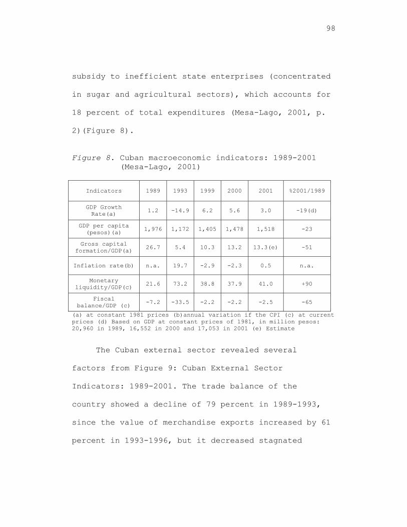
98

subsidy to inefficient state enterprises (concentrated

in sugar and agricultural sectors), which accounts for

18 percent of total expenditures (Mesa-Lago, 2001, p.

2)(Figure 8).

Figure 8. Cuban macroeconomic indicators: 1989-2001

(Mesa-Lago, 2001)

Indicators

1989 1993 1999 2000 2001 %2001/1989

GDP Growth Rate(a)

1.2 -14.9 6.2 5.6 3.0 -19(d)

GDP per capita (pesos)(a)

1,976 1,172 1,405 1,478 1,518 -23

Gross capital formation/GDP(a)

26.7 5.4 10.3 13.2 13.3(e) -51

Inflation rate(b) n.a. 19.7 -2.9 -2.3 0.5 n.a.

Monetary liquidity/GDP(c)

21.6 73.2 38.8 37.9 41.0 +90

Fiscal balance/GDP (c)

-7.2 -33.5 -2.2 -2.2 -2.5 -65

(a) at constant 1981 prices (b)annual variation if the CPI (c) at current prices (d) Based on GDP at constant prices of 1981, in million pesos: 20,960 in 1989, 16,552 in 2000 and 17,053 in 2001 (e) Estimate

The Cuban external sector revealed several

factors from Figure 9: Cuban External Sector

Indicators: 1989-2001. The trade balance of the

country showed a decline of 79 percent in 1989-1993,

since the value of merchandise exports increased by 61

percent in 1993-1996, but it decreased stagnated

99

thereafter; export value was 1.7 billion pesos in

2001, still 68 percent below the 1989 level (Mesa-

Lago, 2001, p. 2) (Figure 9). Imports of goods dropped

75 percent in 1989-1993, but readily rose reaching 5.1

billion pesos in 2001, still 37 percent less than in

1989 (Mesa-Lago, 2001, p. 2)(Figure 9). The trade

balance deficit of goods rose about four fold in 1993-

2001, reaching the historical record of 3.2 billion

pesos in 2000 and 3.4 billion in 2001, 26 percent

higher than the 1989 deficit (Mesa-Lago, 2001, p. 2)

(Figure 9).

One of the major differences between 2001 and

1989 was that Cuba did not benefit from long-term

loans since they had to resort to short-term loans

from foreign banks and other financial institutions by

charging high interest (Mesa-Lago, 2001, p. 3). The

merchandise trade deficit was due to compensation with

a substantial surplus from services, mainly tourism,

and yet the current account balance was negative: -462

million pesos in 1999 (1.8 percent of GDP), -687

million pesos in 2000 (2.5 percent of GDP) and -758

100

million pesos in 2001 (4.4 percent of GDP). These were

the highest deficits since the end of the 1980s and

exhibited a rising trend (Mesa-Lago, 2001, p. 3).

As far as trades, from 1989-2000 (Figure 9) trade

decreased by 50 percentage points, resulting from a

drop in sugar production dropping about one third

while the price of oil jumped 2.5 times creating 18.3

percent deterioration in terms of trades (Mesa-Lago,

2001, p. 3). In 2000, rising oil prices cost $500

million dollars more of a similar volume of oil

imported in 1999 and the increase in prices of sugar

and nickel did not compensate for the high oil prices,

resulting in 22 percent deterioration in terms of

trades (Mesa-Lago, 2001, p. 4). In 2001, the price of

nickel also dropped to 40 percent and prices of sugar

improved, but were still below the 2000 level (prices

of the main exports fell by 25 percent) (Mesa-Lago,

2001, p. 4). Astonishing was in 2000 when Cuba signed

a five-year preferential agreement with Venezuela oil

corporation (PDVSA), which compensated Cuba’s negative

terms of trades by receiving 53,000 barrels of oil

101

daily equivalent to 3 million tons annually, meeting

35 percent of domestic needs (8.6 million tons) (Mesa-

Lago, 2001, p. 4). Cuba was able to receive Venezuela

oil at 25 percent discount and was estimated that the

deal will amount to 2.6 billion U.S. dollar transfer,

as Cuba would resell Venezuelan oil below standard

market price; therefore, earning a sizeable profit in

the international market (Mesa-Lago, 2001, p. 4).

The trade composition of sugar decreased between

73 percent to 27 percent of total export value from

1989-2000, as well as nickel due to world prices,

resulting from 70 percent to 80 percent (about $100

million) in its export values (Mesa-Lago, 2001, p. 4).

Cuba’s trade partners among others include Venezuela,

Spain, Canada, Netherlands, China, Russia, France,

Mexico, and Italy (Mesa-Lago, 2001, p. 4). These

trades partners helped the country in achieving

foreign trades, but the island nation had not reached

full membership status with any of the regional

commercial associations like FTAA (Free Trades of the

Americas) and ACP (Asian, Caribbean and Pacific

102

Groups) limiting the country from expanding its

foreign trades with other countries (Mesa-Lago, 2001).

Cuba’s external debts (Figure 9), jumped from

$6.2 to $11.2 billions in 1989-1998 (mainly due to

accumulation of non paid interests) and slightly

declined to $11.1 billion in 1999 and $10.96 billion

in 2000-2001, because of the depreciation of

currencies that made up most of that debt in relation

to the dollar (Mesa-Lago, 2001, p. 5). Most of Cuba’s

debt had not been paid; even though, the country had

been desperately trying to negotiate short/long term

loans with their Asian, European and Latin American

partners, while making contingencies with foreign

creditors in order to re-establish a credit line with

postpone payments that would be satisfied at a later

date (Mesa-Lago, 2001).

Since 1990 after the collapse of the Soviet Union

and Eastern European block countries, Cuba’s foreign

investment (Figure 9) was visrtually stagnant. In

1995, it was reported at $2.1 billion and in 1998 it

was $2.2 billion (Mesa-Lago, 2001, p. 5). In 2000, it

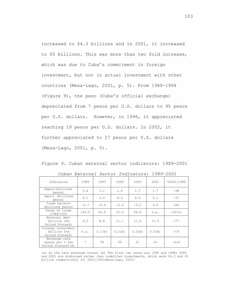
103

increased to $4.3 billions and in 2001, it increased

to $5 billions. This was more than two fold increase,

which was due to Cuba’s commitment in foreign

investment, but not in actual investment with other

countries (Mesa-Lago, 2001, p. 5). From 1989-1994

(Figure 9), the peso (Cuba’s official exchange)

depreciated from 7 pesos per U.S. dollars to 95 pesos

per U.S. dollars. However, in 1996, it appreciated

reaching 19 pesos per U.S. dollars. In 2002, it

further appreciated to 27 pesos per U.S. dollars

(Mesa-Lago, 2001, p. 5).

Figure 9. Cuban external sector indicators: 1989-2001

Cuban External Sector Indicators: 1989-2001

Indicators

1989 1993 1999 2000 2001 %2001/1989

Export(billions pesos) 5.4 1.1 1.4 1.7 1.7 -68

Import (billions pesos)

8.1 2.0 4.3 4.9 5.1 -37

Trade balance (billions pesos) -2.7 -0.9 -2.9 -3.2 3.4 +26

Terms of trade (1989=100)

100.0 54.4 55.9 49.9 n.a. -50(c)

External debt (billion the

United States$) 6.2 8.8 11.1 11.0 11.0 +77

Foreign investment (billion the

United States$) n.a. 2.1(b) 2.2(b) 2.2(b) 2.5(b) +19

Exchange rate (pesos per 1 the

United States$)(a) 7 78 20 21 22 +214

(a) At the rate exchange houses (b) The first two years are 1995 and 1998; 2000 and 2001 are disbursed rather than committed investments, which were $4.3 and $5 billion respectively (c) 2001/1993(Mesa-Lago, 2001)

104

Figure 10 showed the problems that Cuba was

facing with their physical output from 1989-2001

(Mesa-Lago, 2001). A decade after the collapse of

communism and the end of Soviet economic support to

Cuba had not created an economic recovery (Mesa-Lago,

2001). Even the rise of the Cuban Democracy Act of

1992 that began in the early 1990s had not improved

the economy. The Cuban economy declined well into the

21st century (Mesa-Lago, 2001). The indicators in the

physical output showed that the sugar industry

declined since 1989 and, by 2001, the declined output

was reduced to 3.5 million tons, the third lowest

under the revolution. It was 30 percent below the

target of 5 million tons, and 59 percent below the

1989 level (Mesa-Lago, 2001, p. 6). Nickel’s

production decreased 43 percent from 1989-1994, but

with the assistance of investment from Sheritt

International, it surpassed the previous peak in 1996,

and increased to 76,000 tons in 2001, or 62 percent

above the 1989 level (Mesa-Lago, 2001, p. 7). Crude

oil extraction peaked at almost one million tons in

105

1986, but rapidly expanded in 1989-2001, reaching a

record 2.8 million tons due to $450 million in foreign

investment (mainly Sherritt International nickel’s

production), or two thirds of the total investment

(Mesa-Lago, 2001, p. 7). Cuba’s total energy were met

by forty two percent with domestic production, mainly

from bagasse (25 percent) and crude oil (17 percent).

The contribution of natural gas and hydroelectric

power was minimal (0.3 percent), while imported fuel

covered the remaining 58 percent (Mesa-Lago, 2001, p.

7). Cuba did increase its domestic production and

reduced its foreign dependency on oil. However, with

the aid Venezuela was providing Cuba with the sale of

oil at a discount price, Cuba dependency on foreign

oil increased to 77 percent by 2001 (Mesa-Lago, 2001,

p. 7).

In the manufacturing area, both for domestic

consumption and export, the output was drastically

reduced in 1989-1993 but rose thereafter; however, the

reduced output in 2000-2001 was below the 1989 level

in the following manufacturing areas: -87 percent in

106

fertilizers, -78 percent in textiles, -65 percent in

cement and -6 percent in electricity (Mesa-Lago, 2001,

p. 7). Cigars production was 7 percent above the 1989

level based on the international demand and foreign

companies purchasing most of the Cuban cigar industry

(Mesa-Lago, 2001, p. 7). Fishing catch peaked at

244,000 tons in 1986 and by 1989 had declined to

192,000 tons. It was drastically reduced to 88,000 in

1994 but slowly increased to 162,300 tons by 2000

(Mesa-Lago, 2001, p. 7-8). By 2001, the fish

production was 16 percent below the 1989 level and 34

percent below the 1986 peak. The catch in 2001

decreased as follows: 24 percent in tuna, 9 percent in

shrimp, 9 percent in lobster and 24 percent in other

species (Mesa-Lago, 2001, p. 8). Most of the fishing

industry problems resulted from damages inflicted by

several hurricanes in the late 1990s and early 2000,

high indebtedness, bad financial situation, lack of

liquidity both in pesos and in dollars, poor

credibility among the creditors and corruption (Mesa-

Lago & Carmelo, 2001, p. 8).

107

Lastly, Figure 10 provided an insight into

agriculture since the domestic consumption and export

had a history of bad performance. In 2000-2001,

output levels fell compared to 1989. This included a

decline in agriculture: 46 percent in milk, 43 percent

in eggs, 42 percent in rice and 12 percent in citrus

(Mesa-Lago & Carmelo, 2001, p. 8). The drop in dairy

products has been the lack of fodder for cattle. In

addition, chicken imports had fallen to 52 percent

from 1989-2000. The hurricanes affected the citrus

plantations creating a decline in output. This reduced

production-forced Cuba to buy food products from the

United States, including $35 million dollars on rice,

corn and wheat, as well as $600,000 dollars for 10

million eggs (Mesa-Lago, 2001, p. 8). The third

agrarian reforms, introduced in 1993-1994, was unable

to resolve the problems with the agriculture industry,

due to the inefficiency and lack of incentives as Cuba

bought its agricultural output from its farmers at

prices below the market level. This created serious

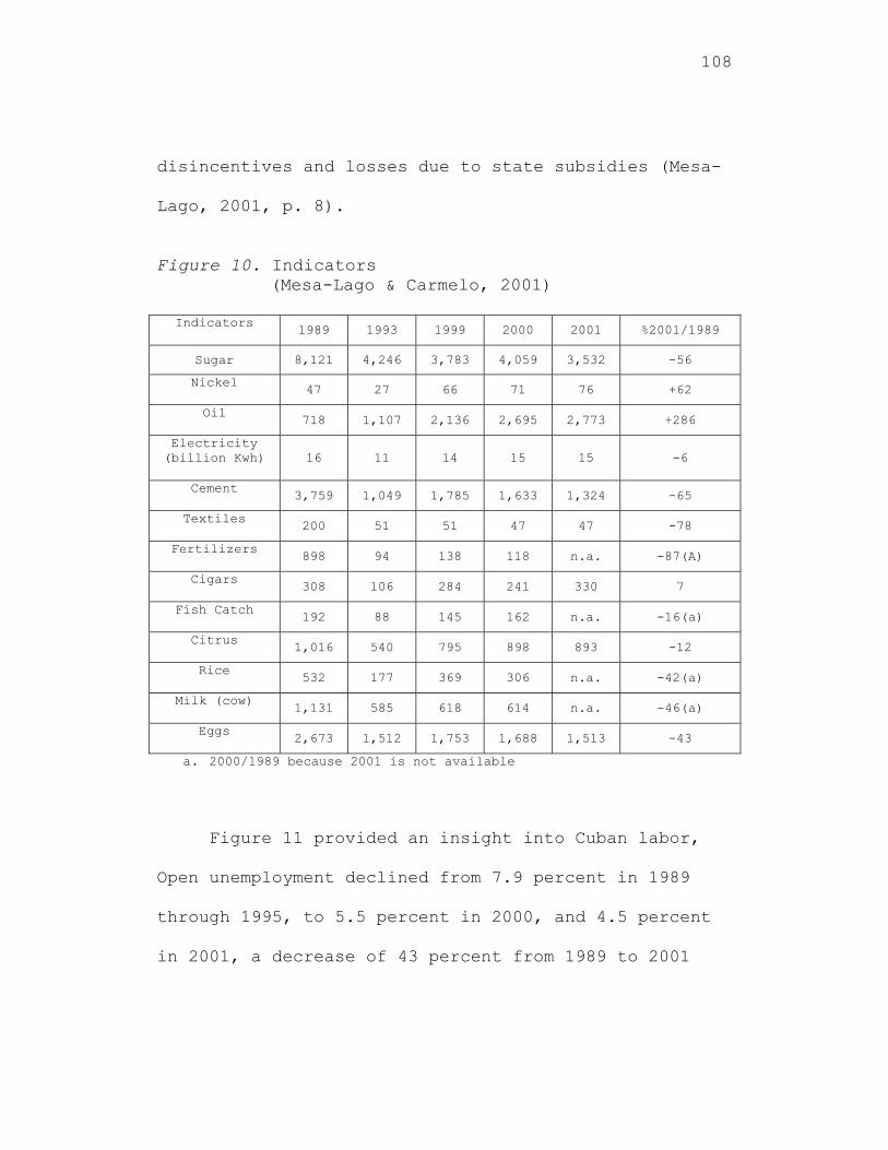
108

disincentives and losses due to state subsidies (Mesa-

Lago, 2001, p. 8).

Figure 10. Indicators

(Mesa-Lago & Carmelo, 2001)

Indicators

1989 1993 1999 2000 2001 %2001/1989

Sugar 8,121 4,246 3,783 4,059 3,532 -56

Nickel

47 27 66 71 76 +62

Oil

718 1,107 2,136 2,695 2,773 +286

Electricity (billion Kwh)

16 11 14 15 15 -6

Cement

3,759 1,049 1,785 1,633 1,324 -65

Textiles

200 51 51 47 47 -78

Fertilizers

898 94 138 118 n.a. -87(A)

Cigars

308 106 284 241 330 7

Fish Catch

192 88 145 162 n.a. -16(a)

Citrus

1,016 540 795 898 893 -12

Rice

532 177 369 306 n.a. -42(a)

Milk (cow)

1,131 585 618 614 n.a. -46(a)

Eggs

2,673 1,512 1,753 1,688 1,513 -43

a. 2000/1989 because 2001 is not available

Figure 11 provided an insight into Cuban labor,

Open unemployment declined from 7.9 percent in 1989

through 1995, to 5.5 percent in 2000, and 4.5 percent

in 2001, a decrease of 43 percent from 1989 to 2001

109

(Mesa-Lago, 2001, p. 8). One of the contributing

factors resulted from state owned business and halting

some of the private sector whose businesses was

catering towards the tourist (Mesa-Lago, 2001). The

Cuban government halted new licenses for tiny

restaurants or so called (paladares), prohibiting

private taxis to take tourist, closing of independent

galleries, allowing only state galleries to operate

under government control and taxing 300 pesos to video

saloons and 800 pesos for rental of dresses (Mesa-

Lago, 2001, p. 9). As a result, the unemployment rate

increased and registered self employed independent

workers decreased from 208,500 at the end of 1995 to

156,600 in 1999 (Mesa-Lago, 2001, p. 9). Social

security wages did increase due to several factors

including virtual universal health care and social

assistance coverage, and low wages of retirement and

pensions. Social security expenditures expanded 14

percent by 2001 from previous years and expected to

continue increasing in the coming years (Mesa-Lago,

2001, p. 9).

110

Real wages’ data were not available for 2000 and

2001. However, there was a recorded decline of about

40 percent from 1989-1999 based on a lack of

connection between wages and real prices which was a

disincentive to labor productivity and an obstacle for

the improvement of the population consumption (Mesa-

Lago, 2001, p. 9). Lastly, infant mortality and

university enrollment according to Figure 11, both

showed considerable decreases during the period of

1989-2001, due to the various factors affecting the

country’s economic slowdown and scarce resources

(Mesa-Lago, 2001, p. 10). In the case of infant

mortality, the rate was 11.1 percent (per 1,000 born

alive) in 1989, falling to 6.4 percent in 1999, rising

to 7.2 percent in 2000 and falling further in 2001 to

6.2 percent, a decline of 44 percent for the whole

period (Mesa-Lago, 2001, p. 10). The contributing

factor dealt with lack of proper nutrition, housing,

water, sanitation and contagious diseases increasing

like acute respiratory, chicken pox, hepatitis,

scarlet fever, syphilis, tuberculosis and typhoid

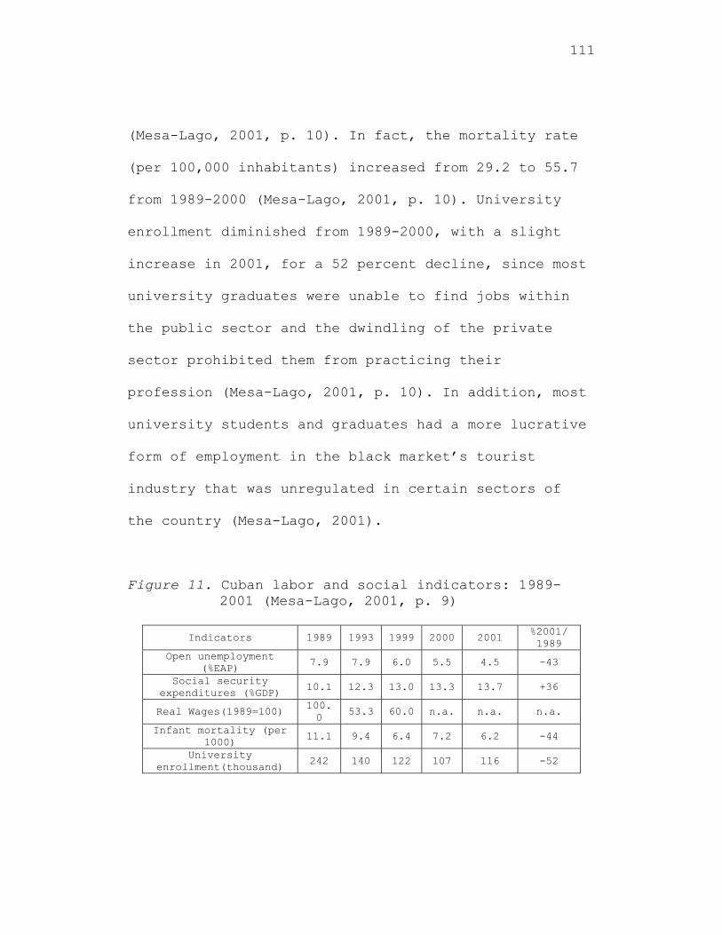
111

(Mesa-Lago, 2001, p. 10). In fact, the mortality rate

(per 100,000 inhabitants) increased from 29.2 to 55.7

from 1989-2000 (Mesa-Lago, 2001, p. 10). University

enrollment diminished from 1989-2000, with a slight

increase in 2001, for a 52 percent decline, since most

university graduates were unable to find jobs within

the public sector and the dwindling of the private

sector prohibited them from practicing their

profession (Mesa-Lago, 2001, p. 10). In addition, most

university students and graduates had a more lucrative

form of employment in the black market’s tourist

industry that was unregulated in certain sectors of

the country (Mesa-Lago, 2001).

Figure 11. Cuban labor and social indicators: 1989-2001 (Mesa-Lago, 2001, p. 9)

Indicators 1989 1993 1999 2000 2001

%2001/ 1989

Open unemployment (%EAP)

7.9 7.9 6.0 5.5 4.5 -43

Social security expenditures (%GDP)

10.1 12.3 13.0 13.3 13.7 +36

Real Wages(1989=100) 100.0

53.3 60.0 n.a. n.a. n.a.

Infant mortality (per 1000)

11.1 9.4 6.4 7.2 6.2 -44

University enrollment(thousand)

242 140 122 107 116 -52

112

Cuba’s Economic Infrastructure, 2001 to 2009

By 2002, Cuban purchased from the United States

Agricultural fair with 288 food producers and

exporters a total of 250 million U.S. dollars, said by

Pedro Alvarez, head of the state-run Alimport food

procurement company (William, 2003, p. A.1). In fact,

according to Pedro Alvarez, Cuba would spend at least

60 percent of its $1 billion in foreign food purchases

on the U.S. products if the U.S. embargo and its

credit restrictions were lifted (William, 2003, p.

A.1).

The United States Chamber of Commerce is also

looking at the opportunity to promote contact in Cuba

despite the legal implications facing most of the

United States firms from the existing embargo and the

Helm-Burton Act, which creates barriers in conducting

trades with Cuba (Mesa-Lago, 2001). Besides the

monthly mailings, corporate members are receiving

special studies on investment in Cuba, the United

States and Cuban laws, and invitations to special

programs and meeting of groups reflecting an

113

optimistic view for future commercial trades with the

island nation (Mesa-Lago, 2001).

AmCham Cuba is a prestigious advisory council

helping the United States business copes in the

relationship and forming bridges in order to access

business view on Cuba’s commercial future. AmCham Cuba

has promoted contacts among persons and MNCs in doing

business with Cuba and establishing a long-term

relationship. In fact, United States Food &

Agribusiness Exhibition has been the first and remains

the only event to be specifically authorized by the

Office of Foreign Assets Control (OFAC) of the United

States Department of the Treasury in conducting (on a

cash basis only) food and agricultural product

business transactions with Cuba (PWN Exhibicon, 2009).

Among the products sold from the United States to Cuba

since 2001, 34 states have been the source for more

than 700,000 metric tons of food products and

agricultural products exported to Cuba under the

provisions of the Trade Sanctions and Export

Enhancement Act (TRSA) of 2000 (PWN Exhibicon, 2009).

114

According to the official report, Cuba’s GDP grew

5 percent in 2004 (Rodriguez, 2004), slightly below

the regional average of 5.5 percent (ECLAC 2004c) UN

Economic Commission for Latin America and the

Caribbean (ECLAC). Cuba’s growth rate in 2004 was

reported at 3 percent; even though, it did not publish

the inflation rate for that fiscal year (Mesa-Lago,

2005, p. 3). According to Cuban Minister of Economics

and Planning, Jose Luis Rodriguez, using the

purchasing power parity of the peso, compared with

other currencies to buy a given basket of goods would

result in calculating a GDP that was 109 percent

higher than using conventional exchange rates (Mesa-

Lago, 2005, p. 3). Rodriguez gave two figures of GDP

growth: one based on the international methodology was

2.6 percent and another adding the value of free

social services and consumption subsidies to the

population was 3.8 percent (Mesa-Lago, 2005, p. 3).

The unemployment rate decreased to 1.9 percent in

2004, reaching an amount to full employment and the

lowest reported in Latin America and the world (Mesa-

115

Lago, 2005, p. 4). The only problem with this data

included a modest expansion of Cuba’s independent

workers during the early 1990s with the Cuban

Democracy Act. The private sector has been contracting

since 2002 due to several problems including the

restructuring of the sugar industry (Mesa-Lago, 2005,

p. 4). Furthermore, there were reports from

independent Cuban Journalist, in which the electricity

crisis of 2004 led to the shutting of 107 industries

and a number of hotels (Mesa-Lago, 2005, p. 4).

Furthermore, sugar harvest was delayed from December

2004, to January 2005, and only 56 sugar mills

operated during that period. To save electricity,

resulting in the working day being reduced by 2.5

hours per week from October 25, 2004, to February 28,

2005, and the number of self employed workers shrank

by 43 percent in 1997-2003 (Mesa-Lago, 2005, p. 4).

As far as the tourist arrivals and revenues

generated during the five-year period from 2000

through 2004, the annual rates of growth slowed down

to 3.1 percent for number of tourists and 3.2 percent

116

for gross revenue (Mesa-Lago, 2005, p. 5). Cuba was

also involved in the discovery of new oil deposits off

shore (Mesa-Lago, 2005, p.6). By 2004, Sheritt-Pebeco

found very promising deposits in Santa Cruz, offshore,

located 55km east of Havana where extraction began of

1,000 tons of crude oil (Mesa-Lago, 2005, p. 7). The

projected path is that Cuba would begin exploration of

offshore drilling in 2006/2007 and well into the

future since there were confirmations of oil in the

cities of Tarara, Guanabo, and Jibacoa, which are

expected to have the same features of the Santa Cruz

deposit (Castro, 2004b). An agreement was made with

Venezuela to supply oil to Cuba. The Venezuela’s state

oil corporation, PDVSA, was to deliver 53,000 barrels

daily, equivalent to 2.7 million tons of oil per

annum, supplying about 30 percent of domestic needs

(Mesa-Lago, 2005, p. 8). By 2004, PDVSA reportedly

increased its delivery from 53,000 to 78,000 barrels

per day (from 2.7 million tons to 4 million tons per

annum) (Mesa-Lago, 2005, p. 9). Cuba’s agreement was

further expanded with Venezuela signing a wider

117

economic and trade agreements with the conditions of

terms to include:

1. Economic integration of both countries, including

the openings of banks and reciprocal banking

credit contracts to facilitate payments in

financial and commercial transactions ((Mesa-

Lago, 2005, p. 9).

2. Elimination of trade tariffs in both countries,

but Cuba benefiting in buying Venezuela oil at

$27 a barrel (about half the current world price)

and keeping 51 percent of ownership in all

foreign investment including Venezuela companies

investing in the country ((Mesa-Lago, 2005, p.

9).

3. Cuba sending to Venezuela tens of thousands of

Cuban physicians, nurses, teachers and sport

trainers who will now be paid by Venezuela

(before this agreement the salaries were paid by

Cuba for reimbursement of supply oil) ((Mesa-

Lago, 2005, p. 9).

118

4. Cuba providing 2,000 annual higher education on

opportunities in energy and award Cubans all the

needed fellowships for research studies, while

Venezuela financing Cuban projects in agriculture

and industry infrastructure, energy, paving of

streets, construction of aqueducts and sewage

treatment facilities for improving Cuba’s economy

through FDI inflow from Venezuela ((Mesa-Lago,

2005, p. 9).

5. Further negotiation between Cuba, Venezuela,

China and Canada’s Sherritt International

Corporation to built thermoelectric plants in

Mariel, Cuba and rebuilding old Soviet oil

refineries in Cienfuegos, Cuba ((Mesa-Lago, 2005,

p. 9).

Cuba’s domestic problems in the agricultural

industry continue well into the 21st Century since the

island nation has been suffering from severe droughts

and in three years (2001-2004), the country was

battered by five major hurricanes (Mesa-Lago, 2005, p.

13). The destruction of the hurricanes totaled $2.15

119

billion in damages to include 54,325 hectares of

crops; 2.4 million animals that had to be moved

causing the reduction of production of pigs and

poultry (800,000 chickens died); 5,360 dwellings

destroyed and 94,896 dwellings damaged (Mesa-Lago,

2005, p. 13-14). The losses also due to drought from

2003 to 2004 were reported at $834 million, including

127,600 cattle dead, 53 million liters of milk lost,

220,000 tons of tubers destroyed, 40,000 tons of

tomatoes destroyed, and 28,160 hectares of other crops

lost and 39,972 hectares damaged (Mesa-Lago, 2005, p.

14). Other key agricultural products were also

significantly affected causing production levels to be

way below 1989 levels. Sugar, rice, coffee and citrus

production fell by 73 percent, 49 percent, 48 percent,

20 percent, respectively. Tobacco production fell by

36 percent. Beef, milk, and egg production also fell

by 54 percent, 46 percent, and 33 percent,

respectively (Mesa-Lago, 2005, p. 14).

Cuba’s biggest crisis occurred in 2004, when the

Antonio Guiteras thermoelectric plant in Matanzas, one

120

of the country’s major power plants, was temporarily

shut down for maintenance due to using domestically

produced heavy oil with high sulfur content (Mesa-

Lago, 2005, p. 16). The shutdown of the plant caused

electric blackouts and severe lack of electricity,

which caused the government to imposed new measures to

include:

1. Shutting down of non-essential activities of

state enterprises (Mesa-Lago, 2005, p. 17).

2. Granting of paid leave to non-essential workers

(Mesa-Lago, 2005, p. 17).

3. Eliminating air conditioning in state offices and

turning off lights early in the night (Mesa-Lago,

2005, p. 17).

4. Scheduling of irrigation activities during the

evening and dawn hours (Mesa-Lago, 2005, p. 17).

5. Closing 4,000 hotel rooms in Havana, Cuba as well

as Varadero, Cayo Largo del Sur, Las Tunas,

Trinidad and Santiago (Mesa-Lago, 2005, p. 17).

6. Shutting down 188 factories during October 2004,

including the largest steel mill (for 220 days),

121

sugar mills, paper producers, and citrus

processing plants (Mesa-Lago, 2005, p. 17).

7. Reducing the length of the workday by 30 minutes

(2.5 hours weekly) for four months, which ended

on February 28, 2005 (Mesa-Lago, 2005, p. 17).

Cuba took other measures in forcing enterprises

and joint ventures to deposit all hard currencies

income in a single account at the BCC (Banco Central

de Cuba) (Mesa-Lago, 2005, p. 39). By depositing the

hard currencies in a single account and requesting its

permission for all transactions involving hard

currency and convertibles pesos from dollars, the BCC

obtained control of credit cards in dollars and

charging them with a ten percent fee, and completely

prohibiting the possessions of dollars (Mesa-Lago,

2005, p. 39).

Cuba’s ill-conceived economic policies have been

unable to recover GDP per capita from the 1989 level.

Nine key agricultural products in 2003 decline from

from 20 percent to 73 percent below their levels of

1989. Production of oil and nickel in six crucial

122

industrial lines (cement, electricity, steel,

textiles, fertilizers and cigars) were from 65 to 85

percent below their pre-crisis levels or remained

stagnant from 1989 level (Mesa-Lago, 2005, p. 41).

Cuba’s new leader, Raul Castro, who took over

power from his ill brother Fidel Castro in 2006, began

opening trades with countries like China. China’s

short-term economic aid may not reduce Cuba’s debt,

which totals $200 million (Mesa-Lago, 2005, p. 44).

However, long term deals with European and Chinese

partners have resume production in the nickel industry

in Cuba. An investment of $500 million of it

ferronickel plant left unfinished by the former Soviet

Union and East European partners totaling $1.3 billion

was implemented by these countries in order to improve

Cuba’s nickel deposit (Mesa-Lago, 2005). These two

projects may not solve the economic problems that the

island is currently experiencing with shortage of food

and basic needs to the Cuban people (Mesa-Lago, 2005).

However, the opening of the United States’ embargo

would be favorable for further trade with the island

123

nation, since currently, the restrictions are still

imposed by the United States Embargo on Cuba. Note

that the embargo does not include food and medicines.

For example, in 2005, agricultural products have made

the United States Cuba’s number one food supplier.

Note that Cuba was the third largest U.S agricultural

importer in Latin America (Mesa-Lago, 2005).

Previous Research on Key Variables

The list of factors previously tested:

According Sawalha (2007) dissertation “The role

of the multinational corporations in economic

development for countries with limited resources”, his

study focused on the role of MNCs in the economic

development using FDI inflow towards countries with

limited resources, identified as developed, developing

and least developing, while making a comparison among

them. His conclusion, through the null hypothesis

indicated countries with higher level of financial

capital, technology, human capital, energy and natural

124

resources, transportation and communication, and

leadership would increase the chances of attracting

more FDI inflows (Sawalha, 2007, p. 106). Furthermore,

the research result confirmed many of the previous

studies that he presented in the literature review in

the field of FDI and its host countries prerequisites,

but added a microlevel perspective testing the

relationship between the elements that constitute the

independent variables and FDI inflows (Sawalha, 2007,

p. 107). According to Pellet (1976, 1986) a system of

labor incentives in the Cuban economy from 1950 to

1970 and socio-economic models and impacts of a small

socialist economy like Cuba, makes reference that the

inappropriate labor incentive was the leading cause to

the deterioration of the Cuban economy. Dr. Pellet

contribution was notable in the area of FDI, since he

was the dissertation chairperson for Dr. Luis I.

Molina-Lacayo and a committee member for Dr. Nabeel N.

Sawalha, two of the reference cited.

125

FDI Implementation in Developing Economies

FDI implementation must have an econometric

analysis using a two-stage estimation procedure, where

the recipient of FDI must have a combination of

governance infrastructure to promote free transparent

markets (Globerman & Shapiro, 2003, p. 3). A country

must also poses a macroeconomic approach in order to

explore those regional distributions of FDI, which

will allow the firm to invest in countries where low

wage levels exist and secure its standing in new and

vibrant markets (Sethi et al., 2003). FDI markets must

be able to provide a geographic advantage by trading

with its FDI recipient countries and should have the

ability to attract technological transfer through the

host country and transfer such information from the

host country via spillover effects (Love, 2003). FDI

has also been linked to corruption, where the levels

of such corruption is either brought from the host

country or created once FDI is transferred by foreign

investors. This impacts the country’s competitive

climate in attracting FDI (Habib & Zurawicki, 2002).

126

FDI must also posses economical and investment

opportunities associated with short and long term

effect in order to allowed a competitive edge for FDI

expansion (Lall, Norman & Featherstone, 2003).

Governance Infrastructure

The importance in preserving a country’s FDI

depends on several factors on legislation and

regulation when transacting and promoting free and

transparent market. FDI preservation would be achieved

through government input, by allowing FDI through

diplomacy and free trade. According to Globerman and

Shapiro (2003), most countries that do not receive FDI

from the United States are small and are classified as

developing countries. Hence, the benefits, in terms of

FDI, are most pronounced for those countries (p. 3).

Moreover, for countries with limited or no FDI,

governance infrastructure is a contributing factor to

the amount received (Globerman & Shapiro, 2003, p. 3).

As governance infrastructure improves and enables a

country in promoting investment decisions with MNCs,

127

the ability of entrepreneurship would be encouraged

and would increase FDI (Globerman & Shapiro, 2003, p.

3). Kaufmann, Kraay, and Zoido-Lobaton (1999) further

explained that one of the governance measures is

estimated by the extent of regulation and market

openness, including tariffs and import control.

Governance infrastructure is correlated directly

and indirectly to the probability of a country

achieving FDI (Globerman & Shapiro, 2003, p. 3). The

results indicated that countries failing to achieve a

minimum threshold of effective governance are unlikely

to receive any of the United States FDI (Globerman &

Shapiro, 2003). Globerman and Shapiro (2003) made

reference that a country with developing economy and a

weak currency is least likely to receive any positive

FDI. It is therefore imperative that those countries

improve their governance in order to create a positive

FDI flows.

128

Technological Advantages

Dunning’s eclectic paradigm, made reference to

the role of technology in expanding FDI. Where a

company has some ownership, a company will set up

production facilities in a foreign country as long as

there are specific advantages in the host country,

which makes FDI preferable to exporting (Love, 2003,

p. 2). Love (2003) illustrates that FDI using

technology is a key element in transferring that

technology that would promote innovation and

development from the home to the host country. Dunning

(1993) often suggested that an increasing share of FDI

is either skill-seeking or efficiency-seeking in high-

technology industries. Such technology can be imposed

in various sectors of the supply and service sector,

such as the transportation and communication industry.

Fosfuri and Motta (1999), questioned the need for

firm-specific advantages to give rise to multinational

activity and provide a formal model of FDI in which

the motivation is not to exploit existing

technological advantages in a foreign country, but to

129

access such technology and transfer it from the host

economy to the investing multinational corporation via

spillover effects (Love, 2003, p. 2). These spillover

effects in accessing technology are beneficial to

developing economies since they lack technological

advances and do not have the capacity in reaching

technological standing, specifically in product

innovation and development (Love, 2003).

Corruption in FDI Markets

FDI and corruption has been analyzed by Habib and

Zurawicki (2002, p. 1), where they referred to

corruption that does not deter in absolute terms.

Recent studies revealed China, Brazil, Thailand, and

Mexico attract large flows of FDI, even though high

levels of corruption exist within these developing

countries (Habib & Zurawicki, 2002). Habib and

Zurawicki (2002) provided an understanding that the

pernicious role of corruption in FDI is important

since it produces bottlenecks, heightens uncertainty,

and raises costs. Furthermore, the corruption between

130

the host country providing FDI assistance to the home

country would be detrimental to the investors of MNCs

doing business abroad (Habib & Zurawicki, 2002, p.1).

The level of corruption would determine how

substantial FDI is perceived and dealt with between

both the host and home country (Habib & Zurawicki

2002, p. 2). Tanzi (1998) referred to corruption

stemming from The World Bank and emphasized the abuse

of public power for private benefit (Habib & Zurawicki

2002, p. 2). However, the benefit also applies to the

private firms engaged in corruption by themselves or

engaged in a business model with the public firms

(Tanzi, 1998). Since most developing countries are

involved in FDI investments, corruption can be

operationalized as an all-inclusive factor, comprising

of bribes, bureaucratic inefficiency, and political

instability in both the private and public sector

(Habib & Zurawicki 2002, p. 3). Foreign investors may

consider corruption morally wrong and may be alienated

from those countries where corruption has reached high

levels (Wir, 2001). An example, several African

131

countries, where corruption is rampant the economy of

these countries are limited in their growth, would

therefore ultimately receive a limited amount of FDI

(Wir, 2001). Furthermore, a corrupt economy does not

provide growth of its economic infrastructure, since

equality for open market and competition is limited,

and bribery may interfere with the ability to transfer

goods in a competitive market (Wir, 2001). Similarly,

corruption does persist in certain cases of FDI,

because some companies can use it to advance their own

interest in an open competitive market (Drabek &

Payne, 1999). Drabek and Payne (1999), indicated that

the use of non-transparency FDI resulted in a negative

impact on the receiving country due to composite

corruption, unstable economic policies, weak and poor

property rights protection, and poor governance.

Corruption can be monitored with the use of

international organizations that allows screening for

corrupt officials, deterring of corrupt environmental

influences using certain watchdogs like Transparency

International (TI) (Habib & Zurawicki, 2002, p. 6).

132

However, in countries where corruption is deeply

ingrained or fully acceptable as a form of business,

bringing organizations like Transparency International

(TI) may not have the pursuing interest to combat

corruption (Habib & Zurawicki, 2002, p. 6).

Former Centrally Planned Economies

Central and Eastern Europe

The business environment in Central and Eastern

Europe has been dramatically altered by the

privatization of state owned enterprises that have

been on going since the fall of communism in 1989

(Fahy et al., 2003, p. 2). According to Thomas (1993),

after the fall of a centrally planned system, a

variety of privatization have evolved in the region

from the sale of state owned assets by government

which has been popular in Hungary to mass ownership

transformation, as it was relatively successful in

Poland and the Czech Republic after 1989 (Fahy et al.,

2003, p. 2). These distinctions were visible when

133

state owned assets were transfer to domestic investors

(insiders) to foreign investors (outsiders) allowing

the movement to attract further FDI and thereby

increasing a firm’s resource base (Fahy et al., 2003,

p. 3). According to Fahy et al. (2003), privatization

was conducted partly or fully with the introduction of

new personnel, the transfer of technology, equipment,

the development of new skills and capabilities through

training and exchange. Firms that were once state

owned and were able to revert and become privatized

through domestic investment, enjoyed greater access to

acquiring resources through foreign assets (Fahy et

al., 2003, p. 4). These foreign assets through FDI

were able to transfer personnel and training. This

most likely resulted in the improvement of capital

intelligence in overcoming the socio-cognitive

obstacles to capability development (Fahy et al.,

2003, p. 4).

Foreign investment by Eastern Central European

countries has shown that countries like Hungary,

Poland, and Czech Republic have the most favorable

134

macroeconomic characteristics for transition to market

based economies and are, therefore, more likely to

receive FDI (Smith & Rebne, 1992, p. 2). Since 1988,

the number of value of the United States investments

in Hungary has increased fourfold. Also, since 1992,

more than three-fourths of all United States

investments in East Central Europe orginated from FDI

(Smith & Rebne, 1992, p. 3). By 1989, demand for FDI

became a focal point of the Hungarian transition,

while Poland with a transition market economy was

pursuing foreign investment by privatization of state

owned firms (Smith & Rebne, 1992, p. 3).

Other social science and managerial fields (such

as political economy and international human resource

management) would include Dunnings’s (1979) eclectic

theory when referring to these East Central European

countries. The dimension of both FDI source and host

nations are addressed by using Dunning’s model and

appear to be subsumed under the omnibus term

foreignness, or, as Dunning has put it, “psychic

distance” (Smith & Rebne, 1992, p. 5).

135

Ownership advantages in FDI includes several

characteristics that a firm must posses such as (1)

proprietorial knowledge, technology, etc.,(2) human

capital, and (3) favored access to production inputs

or markets, as well as (4) FDI implementation from

parent local firms, economies of scales in production

and (5) diversification of risk and access to

production inputs and markets (Smith & Rebne, 1992, p.

5). Poland, using characteristics in developing a

broad presence in Polish banking, focused on

manufacturing, government, office automation and

transportation (Smith & Rebne, 1992, p. 6). Polish

banking in using the first three steps characteristics

of ownership advantages, was able through its joint

venture of Furnel International by Imperial Chemical

(ICL; UK) and Furnel (Poland), to become one of

Poland’s top hard currency earners, and increased the

country’s ability to attract foreign investment (Smith

& Rebne, 1992, p. 6).

In another joint venture between Linde-Technoplyn

(Germany) and Technoplyn-Praha (Czechoslovakia),

136

another state utility privatization, Germany’s Linde

has established a major presence as a producer of

industrial gases formerly provided by the state owned

firm Technoply-Praha (Smith, Rebne, 1992, p. 7). Also,

United Technologies that was well established in

Hungary in 1991 purchased a production site in

Godollo, Hungary, as a basis for foreign sources of

automotive parts (Smith & Rebne, 1992, p. 8). Expected

to cost $10 million to bring the plant into

production, United Technologies was able to create a

domestic market through a FDI wholly owned subsidiary

investment in order minimize expense (Smith & Rebne,

1992, p. 8).

Most notably, the economic transformation of

Poland that began in 1989 has created extraordinary

investment opportunities through foreign firms. The

Polish Agency for Foreign Investment reported that in

2001, 906 firms had made investment of at least one

million dollars, totaling $53.6 in cumulative value

(Deichmann, 2004, p. 1). The acceleration of

investment into Poland has been widely attributed to

137

the reversal of its government’s anti-foreign policies

toward FDI (Michalak, 1993) and Poland’s radical shock

therapy reform program, featuring privatization with a

system of corporate stabilization, liberalization, and

the promotion of inward investment (Balcerowicz,

Blaszczyk, & Dabrowski, 1997, p. 2).

China’s Mixed Economy

China’s mixed economy has grown and is rapidly

growing since its Gross Domestic Product (GDP) has

grown considerably, expected to increase beyond 9.9

percent per annum from 2005 (Energy Information

Administration (EIA), 2006). Inflow of Foreign Direct

Investment (FDI) into China totaled $86.1 billion in

2005, a new record, and twice the level of 2001 (EIA,

2006).

The country’s entry into the World Trade

Organization (WTO) in 2001 and the Chinese

government’s ability in opening trades with foreign

firms have given the country the ability to expand its

economic and investment liberalization. China’s

138

commitment to trades with foreign investment countries

and modifying its once centrally planned economy to a

more revolving mixed economy by opening liberalization

to the private sector has given the country’s a more

profound ways in opening the Chinese economy to

privatization. China’s communist system of government

remains in control of large State Owned Enterprises

(SOEs), many that remain inefficient and unprofitable

(EIA, 2006). China’s major investment has been the

recent oil exploration that began in the 1990s, but

has been fully implemented since 2006. Efforts have

been made to exploit onshore oil and natural gas

fields in the Western providence of Xiniang, Sichuan,

Gansu, and Inner Mongolia, as well as off shore fields

in the Bohay Bay, Pearl River Delta, and South China

Sea (EIA, 2006). China had 18.3 million barrels of

proven oil reserves as of January 2006, and its

consumption totaled 7.4 million barrels of oil per day

that makes the country dependent on foreign oil. The

reserves will undoubtedly provide the country’s

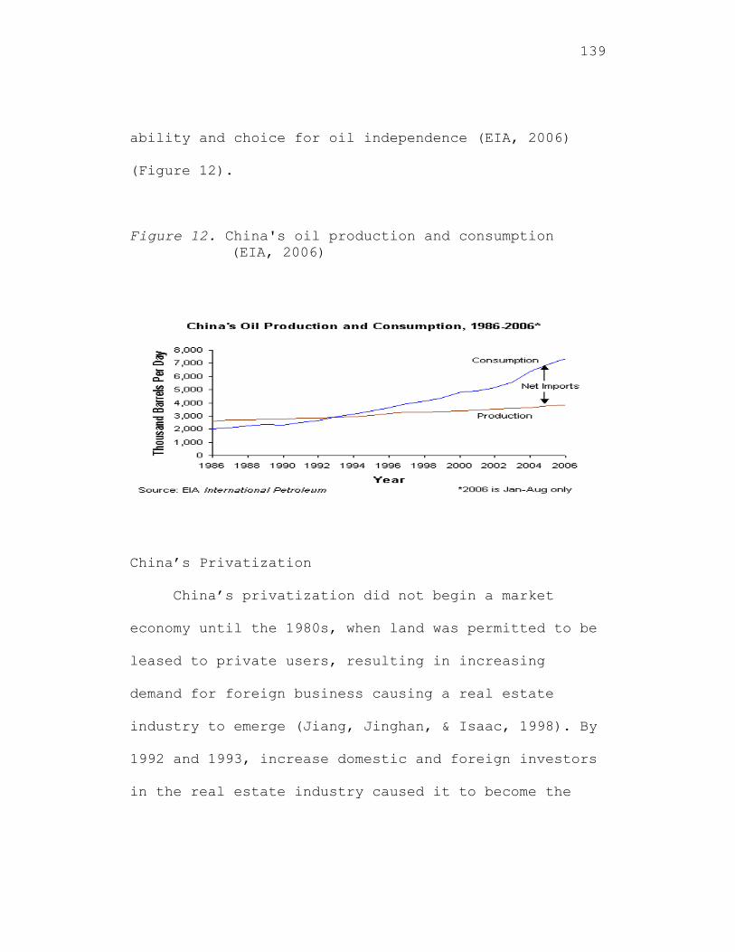
139

ability and choice for oil independence (EIA, 2006)

(Figure 12).

Figure 12. China's oil production and consumption (EIA, 2006)

China’s Privatization

China’s privatization did not begin a market

economy until the 1980s, when land was permitted to be

leased to private users, resulting in increasing

demand for foreign business causing a real estate

industry to emerge (Jiang, Jinghan, & Isaac, 1998). By

1992 and 1993, increase domestic and foreign investors

in the real estate industry caused it to become the

140

leading industry, causing total revenue of the

industry to increase from 52.9 to 113.6 billion yuan

(Jiang, Jinghan, & Isaac, 1998, p. 2). A survey from

the China State Statistical Bureau (1994) stated that

more than 50 million square miles of un-salable houses

located in various cities and rural areas were bought

for about 3 to 6 billion yuan, causing prosperity in

the real estate industry from privatization, which

occurred in cities like Shanghai, Beijing and Tianjin

(Jiang, Jinghan & Isaac, 1998, p. 2). As the real

estate industry emerged, the Central Bank in China

from 1990 and 1991 decreased the country’s interest

rate three times (Jiang, Jinghan, & Isaac, 1998, p.

3). These rates were notable on construction fund

loans which reduced from 11.34 per cent (one-year

loans) and 19.26 per cent (ten-year loans) to 8.64 per

cent and 9.72 per cent to 8.64 per cent and 9.72,

respectively. This reduction in interest rates

benefited the real estate sector (Jiang, Jinghan, &

Isaac, 1998, p. 3). Privatization of the real estate

industry resulted in new investment since the banks

141

were able to extend loans to new domestic and foreign

investors (Jiang, Jinghan, & Isaac, 1998). Such

reforms and readjustments allowed China to expand its

real estate investment, but not at an alarming rate

(Jiang, Jinghan, & Isaac, 1998, p. 4). The interest

rates were increased during the years when China was

transforming its economy from a planned system to a

new process of privatization (Jiang, Jinghan, & Isaac,

1998, p. 4). The slow down caused China to evaluate

its total revenue after 1994.

China was also able to minimize privatization

through the gradual restructuring of the country’s

State Owned Enterprises (SOEs) that began in the mid

1980s (Varouj, Ying, & Jiaping, 2005). According to

Yarrow (1986), Vickers and Yarrow (1991), and Allen

and Gale (1999), less radical steps were taken to

minimize privatization by using methods such as

deregulation and increased competition through State

Owned Enterprises (SOEs), the use of management

performance contracts. There can be effective

solutions for SOE restructuring. The Chinese State

142

Owned Enterprises (SOEs) were able to also modify or

reevaluate the privatization scheme by sharing issue

privatization (SIP) where some, but not all, of the

government’s stake in these firms was sold to

investors through a public share offerings (Varouj,

Ying, & Jiaping, 2005, p. 4). China was able to apply

a gradual approach to SOEs’s reform and was successful

in increasing economic growth and productivity. This

was different from countries like Lithuania, the Czech

Republic and Russia where the reform through mass

privatization has been small since they began reforms

after the collapse of communism (Varouj, Ying, &

Jiaping, 2005, p. 6). According to Groves et al.

(1994), Chinese productivity improved significantly

after 1978, because of the introduction of some basic

incentives like autonomy of the firms in retaining

more of their profits and the incentives of SOEs’s

workers, which were strengthened via bonus payments

and differing work contracts. Because of these

changes, the SOEs’s firms were able to increase

worker’s income and firms investments (Varouj, Ying, &

143

Jiaping, 2005, p. 6). Groves et al. (1995) also

referred to the reform in incentive schemes in the

labor market improving managerial resource allocation

and in turn leading to improvements in SOEs’s

management productivity. In studying Chinese

privatization, Li (1997), documented a significant

increase in the marginal and total factor

productivities of 272 State Owned Enterprises (SOEs).

There was a positive indication where growth in

productivity grew by approximately 90 percent since

there were improved incentives, increase in the

product market competition and a positive outlook for

a more profound allocation of incentive programs

(Varouj, Ying, & Jiaping, 2005, p. 6). In turn,

Shirley and Xu (1998) concluded that incentive

contracts indicated a negative impact on SOEs’s, since

12 SOE contracts had no effect on profitability and

labor productivity, but an adverse effects in the

growth of total factor productivity (Variouj, Ying, &

Jiaping, 2005, p. 6-7). Most notably, Wei, Varela,

D’Souza, and Hassen (2003), conducted a study which

144

evaluated the financial and operating performance of

208 firms in China from 1990-1997. It revealed

significant growth in real output, real assets and

sales efficiency after privatization (Varouj, Ying, &

Jiaping, 2005, p. 7). Furthermore, Sun and Tong (2003)

documented improvements of privatization of SOEs’s

that were significant in earning, sales, and worker’s

productivity for 634 SOEs’s that were privatized

through Share Issue Privatization (SIP) from 1994-1998

(Varouj, Ying, & Jiaping, 2005, p. 7). The impacts of

corporatization on SOE performance were specified in

the following formula:

it =it+it+i+t+i+

where the dependent variable it is the performance

measure for firm i at time t. it is the treatment

variable and is equal to 1 if date t is after

corporatization of firm i, and 0 otherwise, is a

constant, and the i‘s are dummy variables of firms

i’s fixed characteristics including sector, location

and government supervisory level (Varouj, Ying,

145

Jiaping 2005, p. 12). These constant firm

characteristics are omitted in the fixed effect model

since they are captured by the fixed effect term. t

is a set of time dummy variables controlling for

possible variation in the macroeconomic environment

over time (Varouj, Ying,& Jiaping, 2005, p. 12). i is

the firm’s individual characteristics and is included

to control for the unobservable individual effect of

firm i that could be correlated with firm performance

(Varouj, Ying, Jiaping 2005, p. 12). it is the error

term (Varouj, Ying, Jiaping 2005, p. 12).

China’s Technology through FDI

Since 1979, China’s ability to attract advanced

technology through FDI had been notable, with its open

door policy of manufacturing technology in China and

exporting them abroad to foreign countries (Liu,

1995). As a result, a record of FDI has shown a

distinct group of technological investment, classify

as:

146

(1). group of advantages derived from proprietary

advanced technology, such as patented technology and

know how (Shi, 2001, p. 3); and

(2). group of advantages derived from synergies such

as vertical and horizontal integration, which China

was able to promote through technological transfer

across borders through FDI (Shi, 2001, p. 3). China’s

technological transfer was identified through Dunning

(1988a) base theory in a number of location-specific

advantages (LSAs) that led the way to advantages in

the areas of natural resources, cheap land and labor

costs, potential local markets and government policies

that China was able to promote for foreign investors

(Shi, 2001, p. 3). China was able to profit from a

market for technology, which allowed the country to

lure foreign firms to transfer advanced technology

into China (Shi, 2001, p. 6). Therefore, foreign firms

were able to utilize the advanced technology and

allowed in selling their products to local users

through an import substitution scheme in addition to

other preferential treatment (Shi, 2001, p. 6).

147

By establishing a market oriented production

system in China, a market design strategy allowed

parent companies to integrate and better internalize

their labor and land in order to reduce their

production cost and gradually compete in the world’s

market (Shi, 2001, p. 8). Technological transfer, as

was the case in China in the 1980s, created an

innovation through research and development (R&D) over

time, which enhanced the country’s ability to attract

and develop competitiveness of firms over time (Young

& Lan, 1997). R&D also played a crucial role on

technology transfer from parent MNEs that increased

foreign (R&D) affiliates and spillovers to

technological upgrading through domestic privatization

(Young & Lan, 1997). Dunning (1994), makes reference

to China’s technology transfer, assimilation and

innovatory capabilities are increased when the host

country is more attractive as a location for FDI with

an increase value of R&D.

148

Summary

The literature review revealed several theories

important to the research. First, Dunning’s eclectic

theory (1979) was thoroughly explained which

illustrated FDI through internalization of

transferring the products and services away from the

host to a foreign country. In his eclectic theory,

Dunning (1979) referred by investing abroad the

products and services have ownership advantages, along

with technology, humans skills and knowledge.

Dunning’s contribution also provided an explanation

through FDI multinational activities that were driven

by three sets of advantages such as namely ownerships,

location and internatilization (Cantwell & Narula,

2003). The second theory analyze was Hymer’s

Oligopolistic theory (1976), which expanded in the

area of competitive market and demand/supply through

FDI. Hymer’s contribution made it favorable for

countries to expand their FDI support through market

penetration as FDI is transferred from the host to the

FDI recipient country. He made it clear that a well-

149

managed local firm should be able to penetrate foreign

markets with a greater return of good technology that

would enhance in developing countries and emerging

markets (Hymer, 1976). The third theoretical framework

in the study was the inward/outward theories of Adler

and Hufbauer (2008), whose contribution on FDI

economic contribution was discussed. Adler and

Hufbauer (2008) referred than an inward of FDI

requires productive measures of foundation in order to

attract them to develop and less develop economies.

An outward of FDI, Adler and Hufbauer (2008) indicated

through Hymer (1976), that firms must expand abroad by

applying firms-specific skills or technology to a wide

market. The fourth theory discussed was Kotler’s

(1971) marketing development, through his buyer’s

behavior theory, which contrasted production, selling

and customer oriented marketing philosophies, as well

as Megamarketing and how they are transcented through

FDI (Weinstein & Johnson, 1999). The fifth theory

focused on Porter (1996) competitive strategy and

decision making where his discussion was directed at

150

firms responding to competitive market changes as they

transfer their operations through FDI. Porter (1980)

provides an explanation of delivering customer

satisfaction, creating comparable values for superior

profitability and TQM as a strategic positioning once

FDI is considered (Porter 2001, p. 70). Porter (1980)

also provide through his three generic strategies an

explanation of differentiation, overall cost

leadership and focus strategy once firms concentrate

in segments of the market when pursuing FDI (Pearce,

Robinson, 2003).

Cuba’s product and services and its economic

infrastructure from 1959 through 2009 was thoroughly

examined in order to determine the country’s economic

condition for FDI inflow. Data from 1959 through 2009

was able to conclude that the Republic of Cuba is a

viable market for investment by foreign countries.

Lastly, a discussion of FDI implementation in

developing economies and a discussion of former

centrally planned economies in Europe and China was

also discussed since they provided a proxy of FDI and

151

internal restructuring of economic reforms that would

be considered by the Republic of Cuba. They were

beneficial in this study since these formely centrally

planned economies in Eastern Europe and China would

served as a proxy for Cuba’s economic reforms through

FDI.

152

CHAPTER 3

METHODOLOGY

Proposed Research Design and Model

The purpose of this dissertation was to

investigate FDI in the Republic of Cuba in a Post-

Castro Cuba. This study looks at characteristics of

advanced, developing and least developing countries

that affect FDI to the Republic of Cuba (Sawalha,

2007). Such investment of FDI were previously

researched by well-known scholars as Dunning (1977,

1979, 1980, 1988a, 1988b, 1988, 1992, 1993, 1994,

1995, 1998, 2000 & 2003) and Hymer (1970, 1976). FDI

also included marketing strategies by well known

authors, like Adler and Hufbauer (2008), Kotler (1967,

1971, 1972b, 1975, 1986b & 1997) and Porter (1980,

1996, & 2001). This investigation discussed the

research design, data collection, statistical

sampling, hypothesis development, and statistical

testing.

153

In the design of the research, the theory

discussed in Chapters 1 and 2 formulated interest and

ideas about the macro-economic approach to FDI.

Research Questions Examined

The research questions of this study focused on

linking the characteristics of other countries and FDI

to the Republic of Cuba. The questions examined had

explicit determination of relevancy that were

introduced in Chapter I, and thoroughly explained in

Chapter II. Conclusively, the research was used to

analyze the framework of the research questions

regarding the followings: (1) whether the country of

Cuba had the ability to attract FDI (Foreign Direct

Investment) in a post-Castro era; and (2) were

countries willing to invest in Cuba during the onset

of economic conditions and the country’s ultimate

ability in attracting FDI. By identifying these

questions, the statement of the problem established

the goal for this research effort.

154

Primary and Secondary Analysis

According to Leedy & Ormrod, (2004), the layers

that were measured closest to the truth were

considered primary data (p. 89). These consisted of

surveys, particularly useful in describing

characteristics of a large population, as described by

Babbie (2001). Primary data was obtained from data

queries of the World Bank, Freedom House (2000-2001),

International Labor Office Database, World Investment

Report, (UNCTAD, 1998-2008), World Resource Institute

and United Nations for the period, 1998 through 2008

for the 13 countries obtained from the period of 1998-

2008. Based on previous data queries collected,

identified as primary from previous research, the same

data was used in the study as secondary in order to

test the hypotheses.

Secondary data, according to Leedy & Ormrod,

(2004), was farther away from the truth itself, but a

derivative in certain cases from the primary data (p.

89). Secondary data or analysis included various

factors such as academia journals, scholarly materials

155

from well-respected authors, respected journals, and

literature research from recognized scholars in areas

of research and expert testimony. Babbie (2001) also

provided that a secondary analysis was a form of

research where the data was collected, processed by

one researcher and were further re-analyzed with

different purpose by another. The secondary data were

collected for the sample of the 13 countries from the

World Bank, Freedom House (2000-2001), International

Labor Office Database, World Resource Institute and

United Nation’s data queries from 1998-2008. The 13

countries were categorized into three groups: (1)

advanced countries with high GNI Per Capita like the

United States, Japan, Germany, France and Spain;(2)

developing countries with lower and middle level GNI

Per Capita like China, India and the Russian

Federation; and (3) least developed countries (LCD’s)

with low current GNI Per Capita that included Jamaica,

Haiti, Peru, Madagascar and Nepal. The 13 countries

were selected based on their demographics, economic

156

category status and or their FDI relationship with the

Republic of Cuba.

Gathering Method Analysis

Through the gathering method, it should be clear

in the selection process to be essential. The

countries in the advanced category include the United

States, Japan, France, Germany and Spain. The five

countries (United States, Japan, France, Germany and

Spain) were selected based on their past and present

economic trade with the Republic of Cuba (McPherson &

Trumbull, 2007) (Mesa-Lago, 2005). The United States

despite the existing trade embargo with Cuba was a

viable market before 1959. Cuba dependent on the U.S

economy and profited from FDI investment of U.S.

products and services. The second category of

countries includes China, India and the Russian

Federation. All three countries are involved in

significant FDI to Cuba and have previously invested

into the Republic of Cuba (Mesa-Lago, 1979, 2001,

2005). Most notably, the Russian Federation had a long

157

political and economic relationship with Cuba after

the revolution of 1959 and beyond. The third category

of countries includes Jamaica, Haiti, Peru, Madagascar

and Nepal. Jamaica was selected due to its long-

standing trade with Cuba and as a neighboring country

in the Caribbean, both Cuba and Jamaica have built

coalition for positive trade relationship. Haiti,

Peru, Madagascar and Nepal had similar economic

conditions like Cuba, but they would differ in their

economic trade since Cuba has been regulated from

trading in the open market (Journal of Commerce, 1998;

Mesa-Lago, 2005). Haiti, Madagascar and Nepal share

similar economic trades, but not necessarily with

Cuba, while Peru’s natural resources that includes

mining excavation allocates similar characteristics

with Cuba’s natural resources; even though, Cuba’s

deteriorating economy and trade policy excluded other

countries and limited only a few from investing in

Cuba’s natural resources (Mesa-Lago, 2005).

158

Structure of the Variables

The structure of the variables obtained from the

data queries of the 13 countries were grouped into

three different categories. First was advanced

countries and included United States, Japan, France,

Germany and Spain. The second was developing countries

and included China, India and the Russian Federation.

Third as the least developed countries, which included

Jamaica, Haiti, Peru, Madagascar and Nepal. There are

nine independent variables identified as: (1) GNI per

capita, (2) financial capital, (3) level of

technology, (4) human capital, (5) energy and natural

resources, (6) transportation and communication, (7)

market type, (8) environment factors, and (9)

government factors. Additionally, there are fifteen

sub-variables identified as: (1) GNI per capita atlas,

(2) gross fixed capital formation, (3) gross capital

formation, (4) high technology exports, (5) industry

value added, (6) school enrollment, (7) total

unemployment, (8) energy use, (9) fuel imports, (10)

air transport, (11) fixed line and mobile phone

159

subscribers, (12) internet users, (13) merchandise

trade, (14) agriculture value added, and (15) worker’s

remittances and employees’ compensation. The unit of

analysis consisted of the fifteen sub-variable data

grouped into the nine variables for examination

purposes. All of the sub-variable data raw values were

uploaded into an excel file and transferred to a SPSS

program in order to test the hypotheses through a

statistical analysis against the dependent variable.

Dependent Variables

Leedy & Omrod (2004) mentioned that a variable

that is potentially influenced by the independent

variable that “something else” in many cases, is

identified as the dependent variable, because it is

influenced by, and some extent depends on the

independent variable (p. 218). The dependent variable

in this research was the amount of FDI per year

provided to Cuba.

160

The dependent variable FDI to Cuba was obtained from

1998-2007, which remained constant throughout the

testing of the sub-variables from the independent

variables.

Independent Variables

According to Leedy & Omrod (2004), an independent

variable is what a researcher studies as a possible

cause of something else (p. 218). In many cases, this

is one that the researcher directly manipulates is

called an independent variable (Leedy & Omrod, 2004,

p. 218).

The independent variables included:

1. GNI Per Capita: Measured by a country’s Gross

National Income through GNI per capita atlas

based on the country’s domestic monetary system.

2. Financial Capital: Measured by gross fixed

capital formation and gross capital formation

(Dunning, 1988).

161

3. Level of Technology: Measured by high technology

exports and industry, value added (Blomstrom &

Sjoholm, 1999; Dunning, 1988a).

4. Human Capital: Measured by school enrollment and

total unemployment (Sawalha, 2007).

5. Energy and Natural Resources: Measured by the

ratio of know how that offers certain location

specific advantages (LSA) to a foreign country

through energy use and fuel imports (Dunning,

1988a).

6. Transportation and Communication: Measured by the

ratio of total vertical and horizontal

integration of local firms through air transport,

fixed line and mobile phone subscribers and

Internet users (Dunning, 1988a).

7. Market type: The ability to create a marketing

concept through FDI potentials and highly

competitive value chain as measured by

merchandise trade (Dunning, 1988b; Kotler, 1997;

Porter, 1996).

162

8. Environment Factors: Measured by the agriculture

value added, which has a direct and indirect

affect of MNCs conducting FDI ventures (Kobrin,

1976).

9. Governmental Factors: Measured by the worker’s

remittances and employees’ compensation as it

pertains to a country’s labor system.

Hypotheses

The hypotheses were developed based on the independent

variables listed above.

Hypothesis 1 - (GNI per capita)

Hypothesis H01: The level of contribution of

FDI inflow to Cuba is not significantly

related to the GNI per capita for the three

groups of countries.

Hypothesis HA1: The level of contribution of

FDI inflow to Cuba is significantly related to

163

the GNI per capita for the three groups of

countries.

Hypothesis 2 - Financial Capital

Hypothesis H02: The level of contribution of FDI

inflow to Cuba is not significantly related to

the financial capital for the three groups of

countries.

Hypothesis HA2: The level of contribution of FDI

inflow to Cuba is significantly related to the

financial capital for the three groups of

countries.

Hypothesis 3 - Level of Technology

Hypothesis H03: The level of contribution of FDI

inflow to Cuba is not significantly related to

the level of technology for the three groups of

countries.

164

Hypothesis HA3: The level of contribution of FDI

inflow to Cuba is significantly related to the

level of technology for the three groups of

countries.

Hypothesis 4 - Human Capital

Hypothesis H04: The level of contribution of FDI

inflow to Cuba is not significantly related to

human capital for the three groups of

countries.

Hypothesis HA4: The level of contribution of FDI

inflow to Cuba is significantly related to

human capital for the three groups of

countries.

Hypothesis 5 - Energy and Natural Resources

Hypothesis H05: The level of contribution of FDI

inflow to Cuba is not significantly related to

the energy and natural resources for the three

groups of countries.

165

Hypothesis HA5: The level of contribution of FDI

inflow to Cuba is significantly related to the

energy and natural resources for the three

groups of countries.

Hypothesis 6 - Transportation and Communication

Hypothesis H06: The level of contribution of FDI

inflow to Cuba is not significantly related to

the transportation and communication for the

three groups of countries.

Hypothesis HA6: The level of contribution of FDI

inflow to Cuba is significantly related to the

transportation and communication for the three

groups of countries.

Hypothesis 7 - Market Type

Hypothesis H07: The level of contribution of

FDI inflow to Cuba is not significantly

related to the market type for the three

groups of countries.

166

Hypothesis HA7: The level of contribution of

FDI inflow to Cuba is significantly related to

the market type for the three groups of

countries.

Hypothesis 8 - Environment Factors

Hypothesis H08: The level of contribution of

FDI inflow to Cuba is not significantly

related to the environmental factors for the

three groups of countries.

Hypothesis HA8: The level of contribution of

FDI inflow to Cuba is significantly related to

the environmental factors for the three groups

of countries.

Hypothesis 9 - Governmental Factors

Hypothesis H09: The level of contribution of

FDI inflow to Cuba is not significantly

related to the governmental factors for the

three groups of countries.

167

Hypothesis HA9: The level of contribution of

FDI inflow to Cuba is significantly related to

the governmental factors for the three groups

of countries.

Data Collection

The data collected were obtained for 13 countries from

the World Bank, Freedom House (2000-2001),

International Labor Office Database, World Investment

Report, (UNCTAD, 1998-2008), World Resource Institute

and United Nations for the period, 1998 through 2008.

The FDI to Cuba was obtained from UNCTAD (United

Nations Conference on Trade and Development) through

the Harvard College Library website under FDI

statistics.

Reliability of the Data

Leedy and Ormrod (2004) mentioned that the

reliability of the data would draw objective decision

that will undoubtedly conclude drawing to an

appropriate conclusion without biased or subjective

168

terms. The reliability of the data is based on the

accuracy of the data compilation done by World Bank,

Freedom House, International Labor Office Database,

World Investment Report, World Resource Institute and

United Nations. Data are updated yearly.

Validity of the Data

The validity of the data, according to Babbie

(2001), made reference to judgment of an explanation

is to promote credibility. The empirical evidence of

the data obtained revealed that the Republic of Cuba,

as well as the 13 countries in the study belonged to

the United Nations (UN) and the World Bank. Therefore,

data collected from FDI to Cuba and the 13 countries

showed a validity ratio per year since it was

extracted from reputable organizations like the United

Nations (UN) and the World Bank. The data was further

evaluated for validity through other sources to

include Freedom House, International Labor Office,

World Investment Report and the World Resource

Institute database.

169

Originality and Limitations of the Data

In this dissertation, the researcher identified

the following limitations:

1. The researcher understood the limitation in

obtaining information from countries with

advanced, developing, or least developed

economies (Sawalha, 2007).

2. The researcher was limited to 13 countries and

the Republic of Cuba may not have been a

direct correlation to the standard regarding

FDI investment to the Republic of Cuba.

Sampling Techniques

The samples of the 13 countries were grouped into

three different categories, including advanced

countries, developing countries and least developed

countries. The countries classified as advanced

countries were United States, Japan, France, Germany

and Spain. The developing countries were China, India

and the Russian Federation. The least developed

countries were Jamaica, Haiti, Peru, Madagascar and

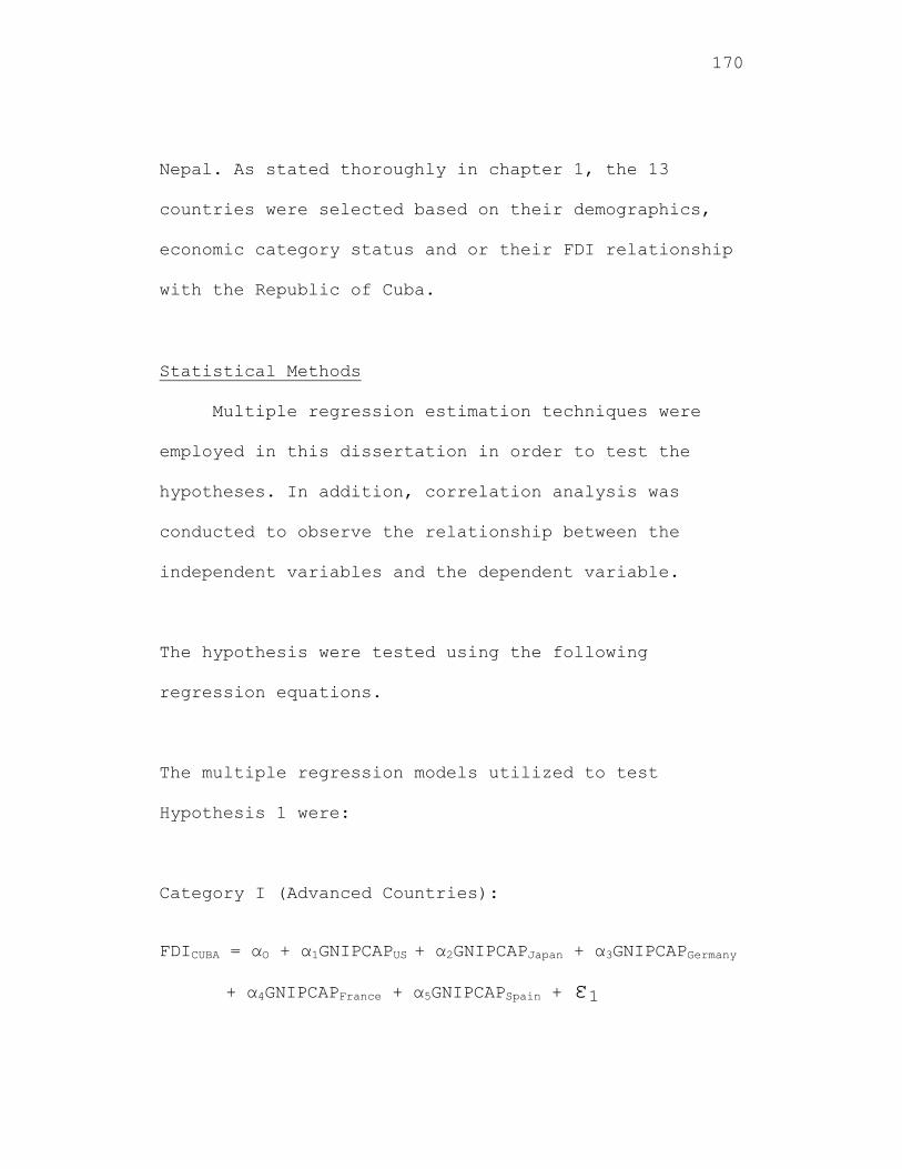
170

Nepal. As stated thoroughly in chapter 1, the 13

countries were selected based on their demographics,

economic category status and or their FDI relationship

with the Republic of Cuba.

Statistical Methods

Multiple regression estimation techniques were

employed in this dissertation in order to test the

hypotheses. In addition, correlation analysis was

conducted to observe the relationship between the

independent variables and the dependent variable.

The hypothesis were tested using the following

regression equations.

The multiple regression models utilized to test

Hypothesis 1 were:

Category I (Advanced Countries):

FDICUBA = αO + α1GNIPCAPUS + α2GNIPCAPJapan + α3GNIPCAPGermany

+ α4GNIPCAPFrance + α5GNIPCAPSpain + ε1

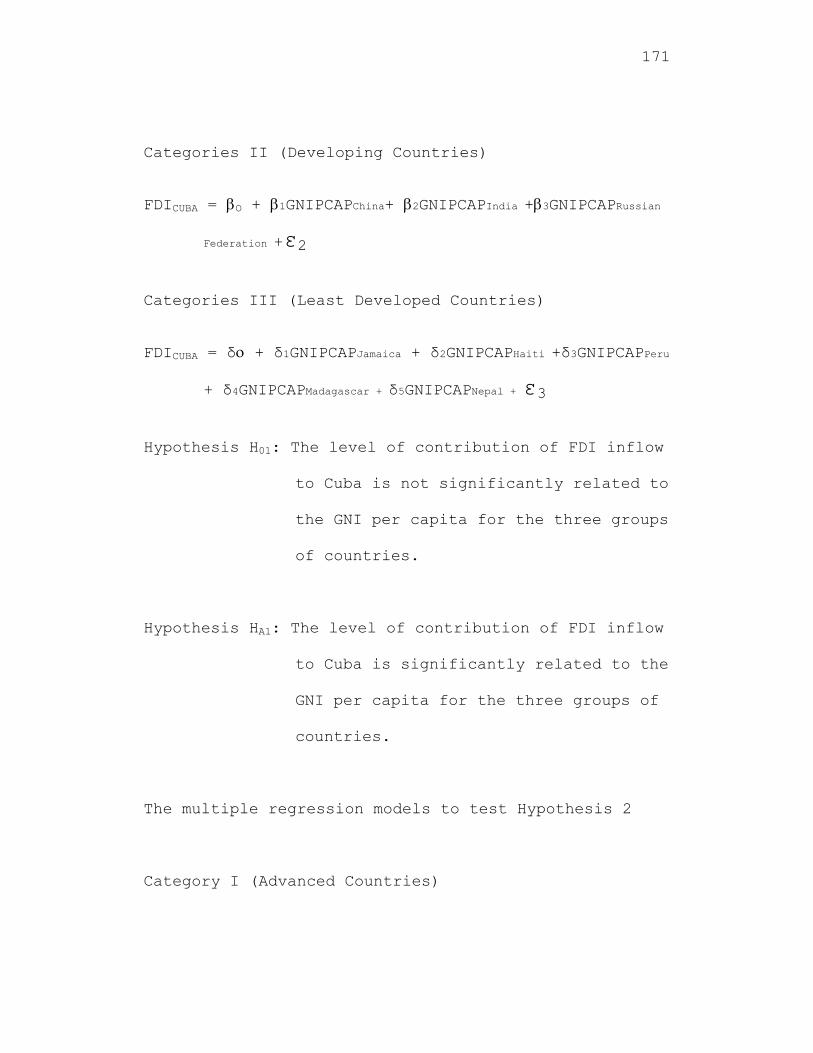
171

Categories II (Developing Countries)

FDICUBA = O + 1GNIPCAPChina+ 2GNIPCAPIndia +3GNIPCAPRussian

Federation +ε2

Categories III (Least Developed Countries)

FDICUBA = δ + δ1GNIPCAPJamaica + δ2GNIPCAPHaiti +δ3GNIPCAPPeru

+ δ4GNIPCAPMadagascar + δ5GNIPCAPNepal + ε3

Hypothesis H01: The level of contribution of FDI inflow

to Cuba is not significantly related to

the GNI per capita for the three groups

of countries.

Hypothesis HA1: The level of contribution of FDI inflow

to Cuba is significantly related to the

GNI per capita for the three groups of

countries.

The multiple regression models to test Hypothesis 2

Category I (Advanced Countries)

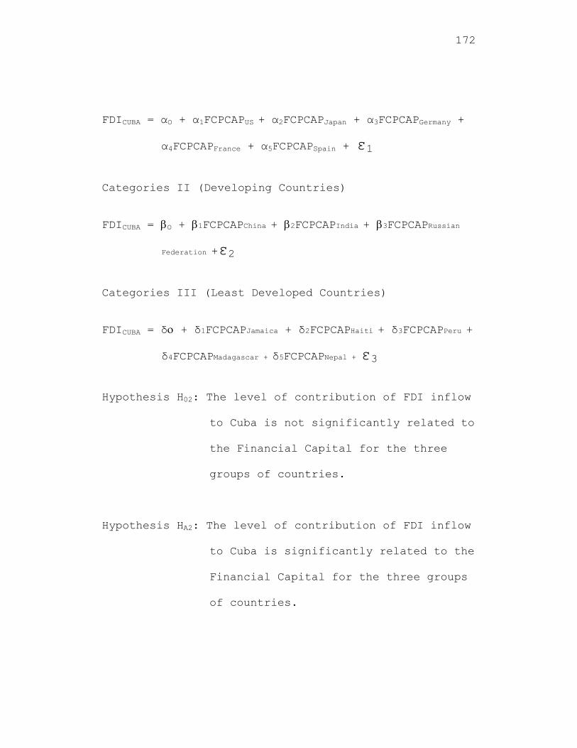
172

FDICUBA = αO + α1FCPCAPUS + α2FCPCAPJapan + α3FCPCAPGermany +

α4FCPCAPFrance + α5FCPCAPSpain + ε1

Categories II (Developing Countries)

FDICUBA = O + 1FCPCAPChina + 2FCPCAPIndia + 3FCPCAPRussian

Federation +ε2

Categories III (Least Developed Countries)

FDICUBA = δ + δ1FCPCAPJamaica + δ2FCPCAPHaiti + δ3FCPCAPPeru +

δ4FCPCAPMadagascar + δ5FCPCAPNepal + ε3

Hypothesis H02: The level of contribution of FDI inflow

to Cuba is not significantly related to

the Financial Capital for the three

groups of countries.

Hypothesis HA2: The level of contribution of FDI inflow

to Cuba is significantly related to the

Financial Capital for the three groups

of countries.

173

The multiple regression models to test Hypothesis 3

Category I (Advanced Countries)

FDICUBA = αO + α1LEVELTECHUS + α2LEVELTECHJapan +

α3LEVELTECHGermany + α4LEVELTECHFrance +

α5LEVELTECHSpain + ε1

Categories II (Developing Countries)

FDICUBA = O + 1LEVELTECHChina + 2LEVELTECHIndia +

3LEVELTECHRussian Federation +ε2

Categories III (Least Developed Countries)

FDICUBA = δ + δ1LEVELTECHJamaica + δ2LEVELTECHHaiti +

δ3LEVELTECHPeru + δ4LEVELTECHMadagascar +

δ5LEVELTECHNepal + ε3

Hypothesis H03: The level of contribution of FDI inflow

to Cuba is not significantly related to

the Level of Technology for the three

groups of countries.

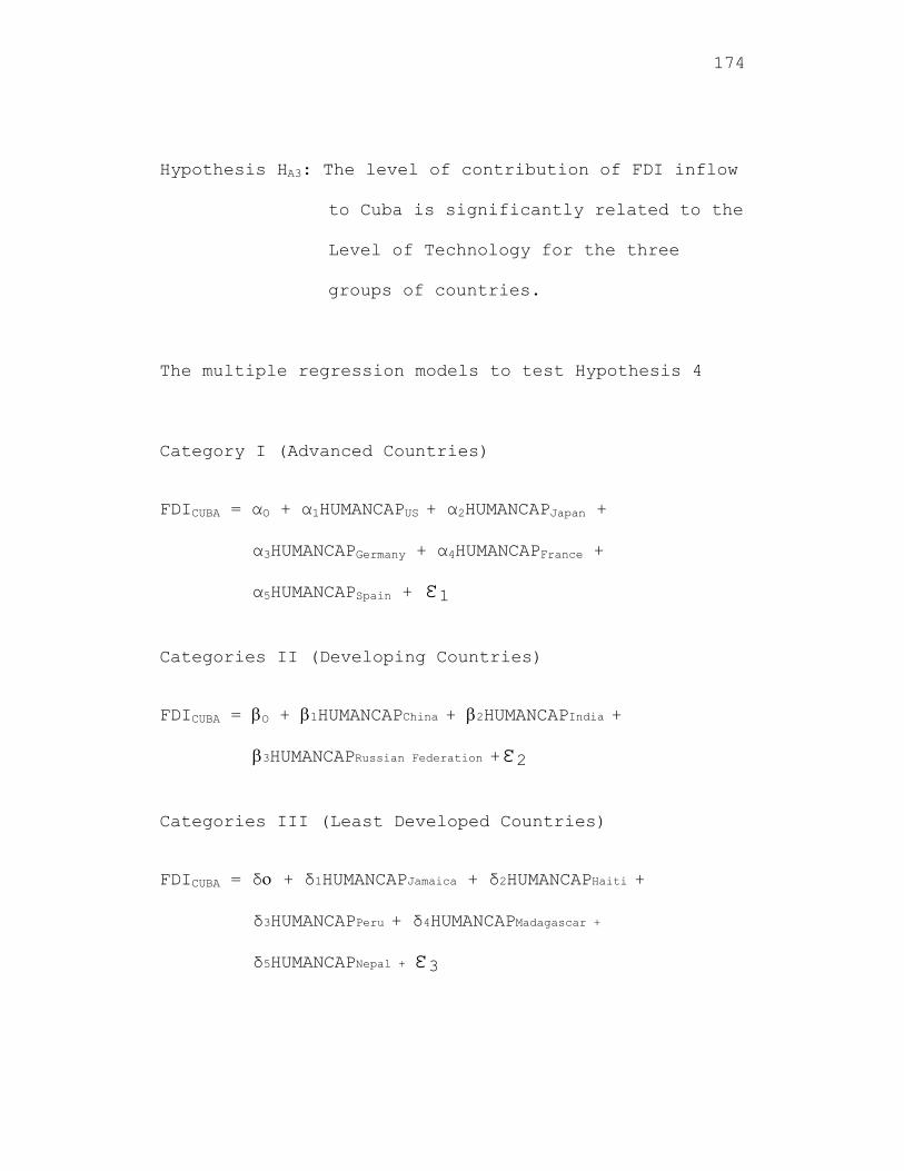
174

Hypothesis HA3: The level of contribution of FDI inflow

to Cuba is significantly related to the

Level of Technology for the three

groups of countries.

The multiple regression models to test Hypothesis 4

Category I (Advanced Countries)

FDICUBA = αO + α1HUMANCAPUS + α2HUMANCAPJapan +

α3HUMANCAPGermany + α4HUMANCAPFrance +

α5HUMANCAPSpain + ε1

Categories II (Developing Countries)

FDICUBA = O + 1HUMANCAPChina + 2HUMANCAPIndia +

3HUMANCAPRussian Federation +ε2

Categories III (Least Developed Countries)

FDICUBA = δ + δ1HUMANCAPJamaica + δ2HUMANCAPHaiti +

δ3HUMANCAPPeru + δ4HUMANCAPMadagascar +

δ5HUMANCAPNepal + ε3

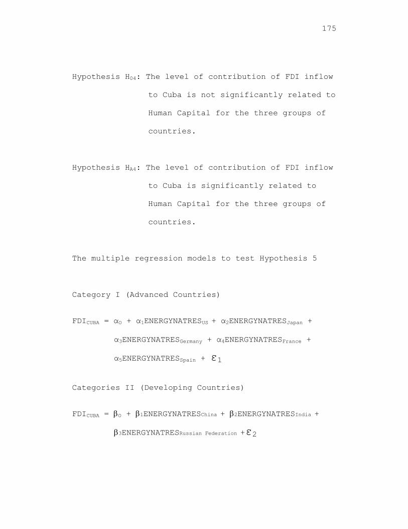
175

Hypothesis H04: The level of contribution of FDI inflow

to Cuba is not significantly related to

Human Capital for the three groups of

countries.

Hypothesis HA4: The level of contribution of FDI inflow

to Cuba is significantly related to

Human Capital for the three groups of

countries.

The multiple regression models to test Hypothesis 5

Category I (Advanced Countries)

FDICUBA = αO + α1ENERGYNATRESUS + α2ENERGYNATRESJapan +

α3ENERGYNATRESGermany + α4ENERGYNATRESFrance +

α5ENERGYNATRESSpain + ε1

Categories II (Developing Countries)

FDICUBA = O + 1ENERGYNATRESChina + 2ENERGYNATRESIndia +

3ENERGYNATRESRussian Federation +ε2

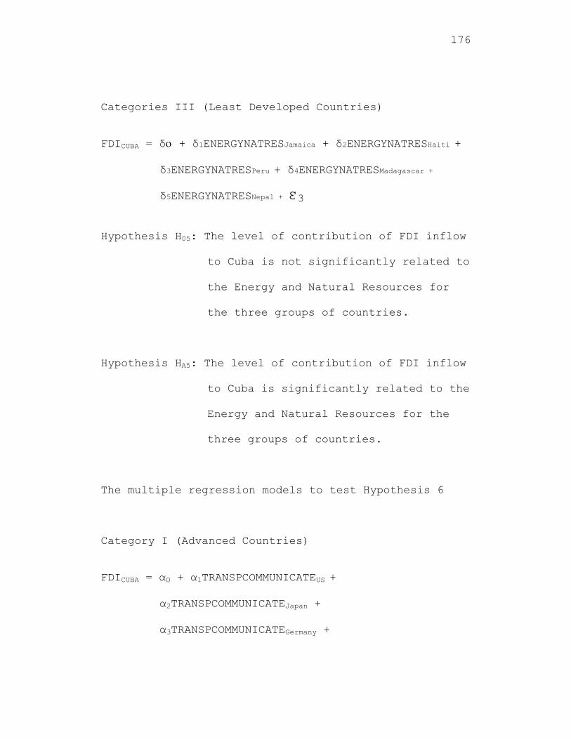
176

Categories III (Least Developed Countries)

FDICUBA = δ + δ1ENERGYNATRESJamaica + δ2ENERGYNATRESHaiti +

δ3ENERGYNATRESPeru + δ4ENERGYNATRESMadagascar +

δ5ENERGYNATRESNepal + ε3

Hypothesis H05: The level of contribution of FDI inflow

to Cuba is not significantly related to

the Energy and Natural Resources for

the three groups of countries.

Hypothesis HA5: The level of contribution of FDI inflow

to Cuba is significantly related to the

Energy and Natural Resources for the

three groups of countries.

The multiple regression models to test Hypothesis 6

Category I (Advanced Countries)

FDICUBA = αO + α1TRANSPCOMMUNICATEUS +

α2TRANSPCOMMUNICATEJapan +

α3TRANSPCOMMUNICATEGermany +

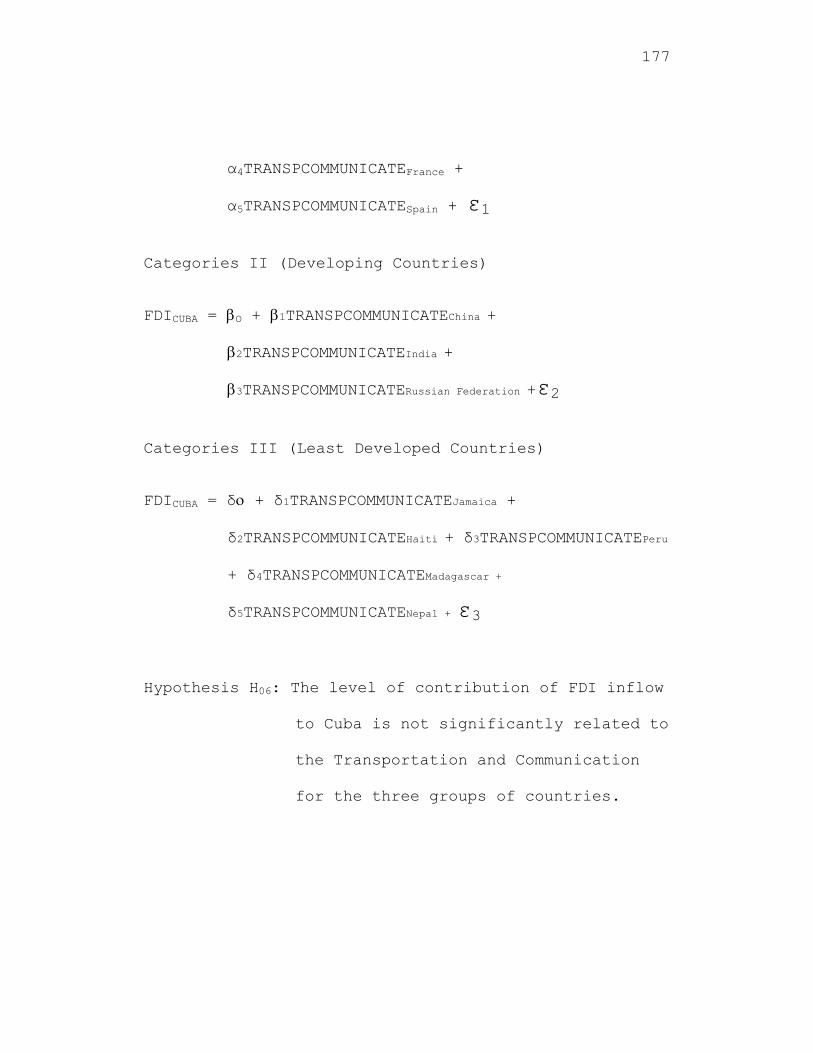
177

α4TRANSPCOMMUNICATEFrance +

α5TRANSPCOMMUNICATESpain + ε1

Categories II (Developing Countries)

FDICUBA = O + 1TRANSPCOMMUNICATEChina +

2TRANSPCOMMUNICATEIndia +

3TRANSPCOMMUNICATERussian Federation +ε2

Categories III (Least Developed Countries)

FDICUBA = δ + δ1TRANSPCOMMUNICATEJamaica +

δ2TRANSPCOMMUNICATEHaiti + δ3TRANSPCOMMUNICATEPeru

+ δ4TRANSPCOMMUNICATEMadagascar +

δ5TRANSPCOMMUNICATENepal + ε3

Hypothesis H06: The level of contribution of FDI inflow

to Cuba is not significantly related to

the Transportation and Communication

for the three groups of countries.

178

Hypothesis HA6: The level of contribution of FDI inflow

to Cuba is significantly related to the

Transportation and Communication for

the three groups of countries.

The multiple regression models to test Hypothesis 7

Category I (Advanced Countries)

FDICUBA = αO + α1MARKETTYPEUS + α2MARKETTYPEJapan +

α3MARKETTYPEGermany + α4MARKETTYPEFrance +

α5MARKETTYPESpain + ε1

Categories II (Developing Countries)

FDICUBA = O + 1MARKETTYPEChina + 2MARKETTYPEIndia +

3MARKETTYPERussian Federation +ε2

Categories III (Least Developed Countries)

FDICUBA = δ + δ1MARKETTYPEJamaica + δ2MARKETTYPEHaiti +

δ3MARKETTYPEPeru + δ4MARKETTYPEMadagascar +

δ5MARKETTYPENepal + ε3

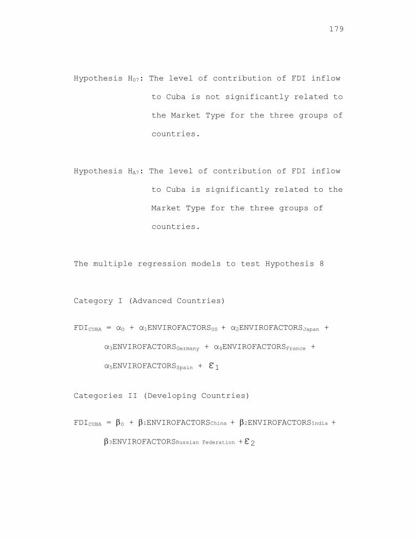
179

Hypothesis H07: The level of contribution of FDI inflow

to Cuba is not significantly related to

the Market Type for the three groups of

countries.

Hypothesis HA7: The level of contribution of FDI inflow

to Cuba is significantly related to the

Market Type for the three groups of

countries.

The multiple regression models to test Hypothesis 8

Category I (Advanced Countries)

FDICUBA = αO + α1ENVIROFACTORSUS + α2ENVIROFACTORSJapan +

α3ENVIROFACTORSGermany + α4ENVIROFACTORSFrance +

α5ENVIROFACTORSSpain + ε1

Categories II (Developing Countries)

FDICUBA = O + 1ENVIROFACTORSChina + 2ENVIROFACTORSIndia +

3ENVIROFACTORSRussian Federation +ε2

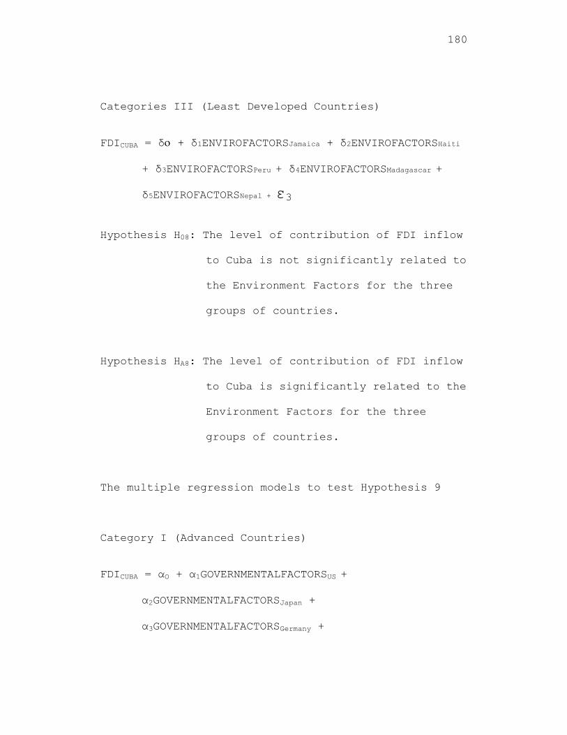
180

Categories III (Least Developed Countries)

FDICUBA = δ + δ1ENVIROFACTORSJamaica + δ2ENVIROFACTORSHaiti

+ δ3ENVIROFACTORSPeru + δ4ENVIROFACTORSMadagascar +

δ5ENVIROFACTORSNepal + ε3

Hypothesis H08: The level of contribution of FDI inflow

to Cuba is not significantly related to

the Environment Factors for the three

groups of countries.

Hypothesis HA8: The level of contribution of FDI inflow

to Cuba is significantly related to the

Environment Factors for the three

groups of countries.

The multiple regression models to test Hypothesis 9

Category I (Advanced Countries)

FDICUBA = αO + α1GOVERNMENTALFACTORSUS +

α2GOVERNMENTALFACTORSJapan +

α3GOVERNMENTALFACTORSGermany +

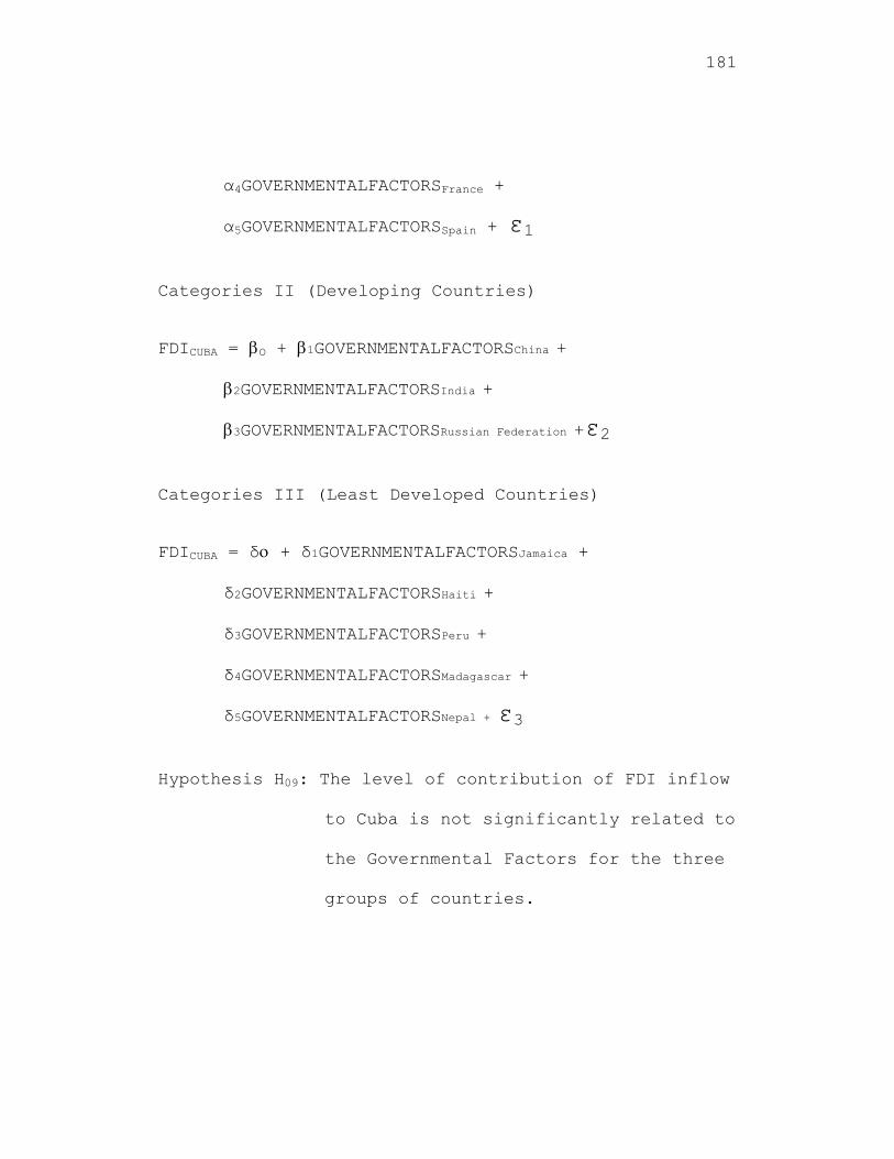
181

α4GOVERNMENTALFACTORSFrance +

α5GOVERNMENTALFACTORSSpain + ε1

Categories II (Developing Countries)

FDICUBA = O + 1GOVERNMENTALFACTORSChina +

2GOVERNMENTALFACTORSIndia +

3GOVERNMENTALFACTORSRussian Federation +ε2

Categories III (Least Developed Countries)

FDICUBA = δ + δ1GOVERNMENTALFACTORSJamaica +

δ2GOVERNMENTALFACTORSHaiti +

δ3GOVERNMENTALFACTORSPeru +

δ4GOVERNMENTALFACTORSMadagascar +

δ5GOVERNMENTALFACTORSNepal + ε3

Hypothesis H09: The level of contribution of FDI inflow

to Cuba is not significantly related to

the Governmental Factors for the three

groups of countries.

182

Hypothesis HA9: The level of contribution of FDI inflow

to Cuba is significantly related to the

Governmental Factors for the three

groups of countries.

Summary

This chapter illustrated the research methodology

design for the study, which was further analyzed by

proposed research and design model. The research

questions were examined, describing the primary and

secondary analysis, illustrating the gathering method

and the structure of the variables. Furthermore, the

operation of the dependent and independent variables,

the research hypotheses, a measure of the data

collection with sampling techniques and statistical

methods in the manner the sample was selected and

discussed in the research. Chapter 4 presents further

evidence of the research sample and the analytical

examination of the data. Furthermore, the result of

the statistical examination of the research hypothesis

183

was tested in order to verify if the null hypothesis

would either be accepted or rejected.

184

CHAPTER 4

ANALYSIS AND FINDINGS

Introduction

This chapter provides a discussion of the data,

data analysis and the research findings. This study

tested the variables from 13 non-oil producing

countries that can impact FDI inflow to Cuba. The

variables were: GNI per capita, Financial Capital,

Level of Technology, Human Capital, Energy and Natural

Resources, Transportation and Communication, Market

Type, Environment Factors and Governmental Factors.

The 13 non-oil producing countries were selected based

on their demographics, economic category status and or

their FDI relationship with the Republic of Cuba.

Data

The data described in Chapter 3 were obtained for

13 countries from the World Bank, Freedom House (2000-

185

2001), International Labor Office Database, World

Investment Report, (UNCTAD, 1998-2008), World Resource

Institute and United Nations for the period, 1998

through 2008. The samples of countries were grouped

into three different categories, including advanced

countries, developing countries and least developed

countries. The countries classified as advanced

countries were United States, Japan, France, Germany

and Spain. The developing countries were China, India

and the Russian Federation. The least developed

countries were Jamaica, Haiti, Peru, Madagascar and

Nepal. All hypotheses were tested using SPSS.

Results for Hypothesis 1

FDI to Cuba was the dependent variable. For the

advanced countries, the independent variables were GNI

per capita for the United States, Japan, Germany,

France and Spain (Sawalha, 2007). The independent

variables for the developing countries were GNI per

capita for China, India and the Russian Federation

(Sawalha, 2007). The independent variables for the

186

Least Developed Countries (LCD’s) were GNI per capita

for Jamaica, Haiti, Peru, Madagascar and Nepal. The

Republic of Cuba’s GNI per capita was not included in

the model as there were only three data points.

The correlation coefficient for GNI per Capita Atlas

and GNI per capita PPP for the United States was

0.9926, implying that these measures were highly

correlated. Similar results were found for GNI per

capita for the other countries. Hence, Hypothesis 1

was only tested with GNI per Capita Atlas. The

difference between GNI per Capita Atlas and PPP is

based on the measurement of GNI per Capita. GNI per

capita Atlas was based on the country’s domestic

monetary measurement, while GNI per PPP was based on

the international monetary measurement (worldbank

report, 2008).

The first hypothesis to be tested is:

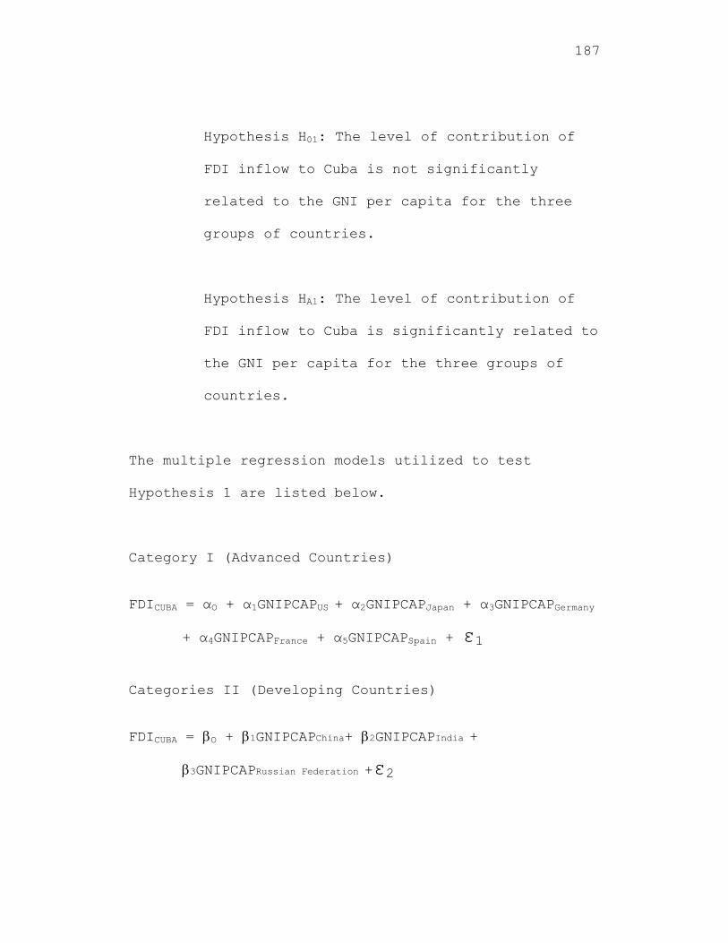
187

Hypothesis H01: The level of contribution of

FDI inflow to Cuba is not significantly

related to the GNI per capita for the three

groups of countries.

Hypothesis HA1: The level of contribution of

FDI inflow to Cuba is significantly related to

the GNI per capita for the three groups of

countries.

The multiple regression models utilized to test

Hypothesis 1 are listed below.

Category I (Advanced Countries)

FDICUBA = αO + α1GNIPCAPUS + α2GNIPCAPJapan + α3GNIPCAPGermany

+ α4GNIPCAPFrance + α5GNIPCAPSpain + ε1

Categories II (Developing Countries)

FDICUBA = O + 1GNIPCAPChina+ 2GNIPCAPIndia +

3GNIPCAPRussian Federation +ε2

188

Categories III (Least Developed Countries)

FDICUBA = δ + δ1GNIPCAPJamaica + δ2GNIPCAPHaiti +

δ3GNIPCAPPeru + δ4GNIPCAPMadagascar + δ5GNIPCAPNepal + ε3

The results were presented for the independent

variables measuring GNI Per Capita Atlas for each of

the three categories of countries.

Results for GNI Per Capita

Results for Category I (Advanced Countries) Using the Independent Variable, GNI Per Capita Atlas

The multiple regression analysis, with FDI to

Cuba as the dependent variable and GNI Per Capita

Atlas for the advanced countries, the United States,

Japan, Germany, France and Spain as the independent

variables, did not revealed any significant

relationships. From the ANOVA, the F-value = 4.038

with a p-value = 0.100 implying that the model was not

significant (Table 1). This was also seen from the

189

multiple regression analysis where the beta

coefficients were not significant, implying the null

hypothesis was not rejected for these countries (Table

2). Therefore, there was no significant correlation

between the FDI to Cuba and the GNI Per Capita Atlas

for these advanced countries, the United States,

Japan, Germany, France and Spain. This result was

surprising as Germany, France and Spain had been

providing significant FDI to Cuba. From the

collinearity diagnostics, the variance inflation

factors (VIF) were 227.125, 9.760, 2952.463, 4482.878

and 636.668 for the United States, Japan, Germany,

France and Spain, respectively, implying a major

multicollinearity problem. (A VIF greater than 5 is

usually an indication of a multicollinearity problem.)

This implies that the five independent variables are

highly correlated and cannot be utilized for multiple

regression analysis. A correlation analysis further

reinforced this position. Simple linear regression was

conducted for each of these countries.

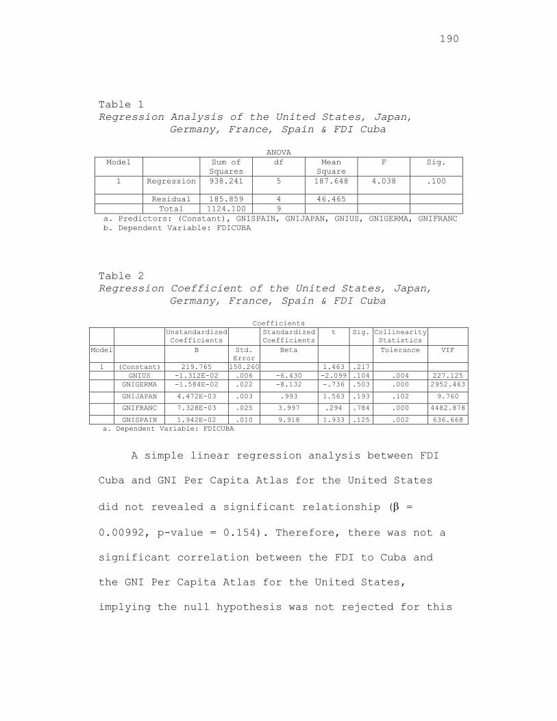
190

Table 1 Regression Analysis of the United States, Japan,

Germany, France, Spain & FDI Cuba

ANOVA Model Sum of

Squares df Mean

Square F Sig.

1 Regression 938.241 5 187.648 4.038 .100

Residual 185.859 4 46.465 Total 1124.100 9

a. Predictors: (Constant), GNISPAIN, GNIJAPAN, GNIUS, GNIGERMA, GNIFRANC b. Dependent Variable: FDICUBA

Table 2 Regression Coefficient of the United States, Japan,

Germany, France, Spain & FDI Cuba

Coefficients Unstandardized

Coefficients Standardized

Coefficientst Sig. Collinearity

Statistics

Model B Std. Error

Beta Tolerance VIF

1 (Constant) 219.765 150.260 1.463 .217 GNIUS -1.312E-02 .006 -6.430 -2.099 .104 .004 227.125 GNIGERMA -1.584E-02 .022 -8.132 -.736 .503 .000 2952.463

GNIJAPAN 4.472E-03 .003 .993 1.563 .193 .102 9.760

GNIFRANC 7.328E-03 .025 3.997 .294 .784 .000 4482.878

GNISPAIN 1.942E-02 .010 9.918 1.933 .125 .002 636.668 a. Dependent Variable: FDICUBA

A simple linear regression analysis between FDI

Cuba and GNI Per Capita Atlas for the United States

did not revealed a significant relationship ( =

0.00992, p-value = 0.154). Therefore, there was not a

significant correlation between the FDI to Cuba and

the GNI Per Capita Atlas for the United States,

implying the null hypothesis was not rejected for this

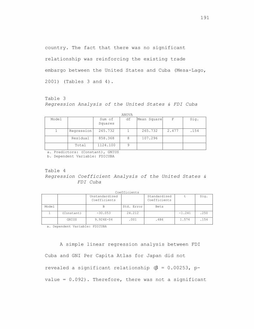
191

country. The fact that there was no significant

relationship was reinforcing the existing trade

embargo between the United States and Cuba (Mesa-Lago,

2001) (Tables 3 and 4).

Table 3 Regression Analysis of the United States & FDI Cuba

ANOVA Model Sum of

Squares df Mean Square F Sig.

1 Regression 265.732 1 265.732 2.477 .154

Residual 858.368 8 107.296

Total 1124.100 9

a. Predictors: (Constant), GNIUS b. Dependent Variable: FDICUBA Table 4 Regression Coefficient Analysis of the United States &

FDI Cuba

Coefficients Unstandardized

Coefficients Standardized

Coefficients t Sig.

Model B Std. Error Beta

1 (Constant) -30.053 24.212 -1.241 .250

GNIUS 9.924E-04 .001 .486 1.574 .154

a. Dependent Variable: FDICUBA

A simple linear regression analysis between FDI

Cuba and GNI Per Capita Atlas for Japan did not

revealed a significant relationship ( = 0.00253, p-

value = 0.092). Therefore, there was not a significant

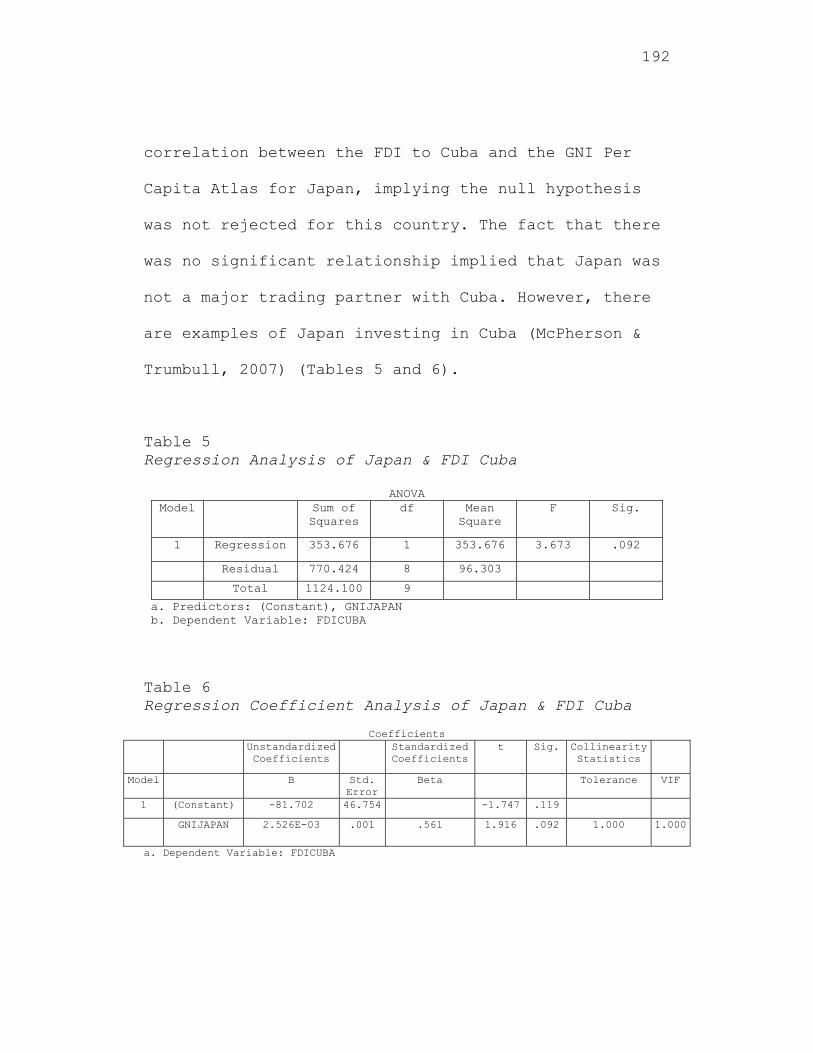
192

correlation between the FDI to Cuba and the GNI Per

Capita Atlas for Japan, implying the null hypothesis

was not rejected for this country. The fact that there

was no significant relationship implied that Japan was

not a major trading partner with Cuba. However, there

are examples of Japan investing in Cuba (McPherson &

Trumbull, 2007) (Tables 5 and 6).

Table 5 Regression Analysis of Japan & FDI Cuba

ANOVA Model Sum of

Squares df Mean

Square F Sig.

1 Regression 353.676 1 353.676 3.673 .092

Residual 770.424 8 96.303

Total 1124.100 9

a. Predictors: (Constant), GNIJAPAN b. Dependent Variable: FDICUBA Table 6 Regression Coefficient Analysis of Japan & FDI Cuba

Coefficients Unstandardized

Coefficients Standardized

Coefficientst Sig. Collinearity

Statistics

Model B Std. Error

Beta Tolerance VIF

1 (Constant) -81.702 46.754 -1.747 .119

GNIJAPAN 2.526E-03 .001 .561 1.916 .092 1.000 1.000

a. Dependent Variable: FDICUBA

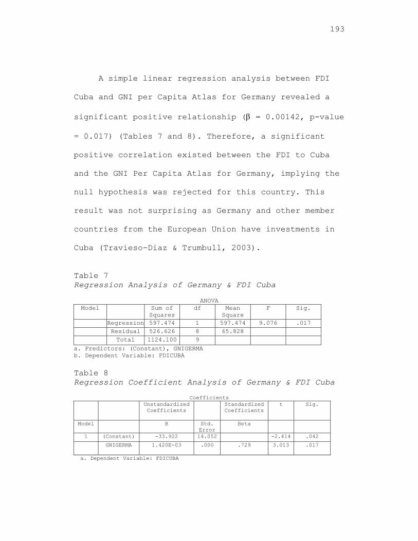
193

A simple linear regression analysis between FDI

Cuba and GNI per Capita Atlas for Germany revealed a

significant positive relationship ( = 0.00142, p-value

= 0.017) (Tables 7 and 8). Therefore, a significant

positive correlation existed between the FDI to Cuba

and the GNI Per Capita Atlas for Germany, implying the

null hypothesis was rejected for this country. This

result was not surprising as Germany and other member

countries from the European Union have investments in

Cuba (Travieso-Diaz & Trumbull, 2003).

Table 7 Regression Analysis of Germany & FDI Cuba

ANOVA Model Sum of

Squares df Mean

Square F Sig.

Regression 597.474 1 597.474 9.076 .017 Residual 526.626 8 65.828 Total 1124.100 9

a. Predictors: (Constant), GNIGERMA b. Dependent Variable: FDICUBA

Table 8 Regression Coefficient Analysis of Germany & FDI Cuba

Coefficients Unstandardized

Coefficients Standardized

Coefficients t Sig.

Model B Std. Error

Beta

1 (Constant) -33.922 14.052 -2.414 .042

GNIGERMA 1.420E-03 .000 .729 3.013 .017

a. Dependent Variable: FDICUBA

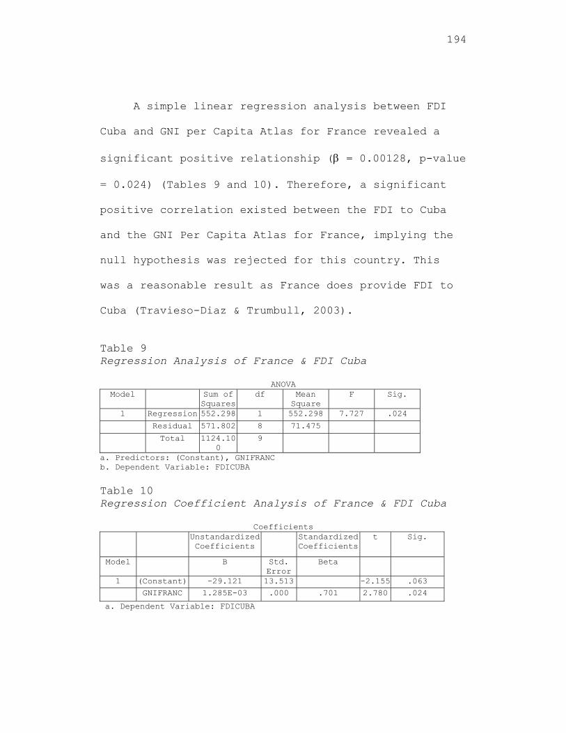
194

A simple linear regression analysis between FDI

Cuba and GNI per Capita Atlas for France revealed a

significant positive relationship ( = 0.00128, p-value

= 0.024) (Tables 9 and 10). Therefore, a significant

positive correlation existed between the FDI to Cuba

and the GNI Per Capita Atlas for France, implying the

null hypothesis was rejected for this country. This

was a reasonable result as France does provide FDI to

Cuba (Travieso-Diaz & Trumbull, 2003).

Table 9 Regression Analysis of France & FDI Cuba

ANOVA Model Sum of

Squaresdf Mean

Square F Sig.

1 Regression 552.298 1 552.298 7.727 .024

Residual 571.802 8 71.475

Total 1124.100

9

a. Predictors: (Constant), GNIFRANC b. Dependent Variable: FDICUBA

Table 10 Regression Coefficient Analysis of France & FDI Cuba

Coefficients Unstandardized

Coefficients Standardized

Coefficientst Sig.

Model B Std. Error

Beta

1 (Constant) -29.121 13.513 -2.155 .063

GNIFRANC 1.285E-03 .000 .701 2.780 .024

a. Dependent Variable: FDICUBA

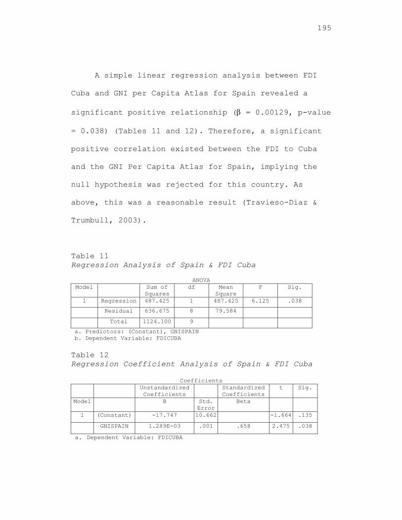
195

A simple linear regression analysis between FDI

Cuba and GNI per Capita Atlas for Spain revealed a

significant positive relationship ( = 0.00129, p-value

= 0.038) (Tables 11 and 12). Therefore, a significant

positive correlation existed between the FDI to Cuba

and the GNI Per Capita Atlas for Spain, implying the

null hypothesis was rejected for this country. As

above, this was a reasonable result (Travieso-Diaz &

Trumbull, 2003).

Table 11 Regression Analysis of Spain & FDI Cuba

ANOVA Model Sum of

Squares df Mean

Square F Sig.

1 Regression 487.425 1 487.425 6.125 .038

Residual 636.675 8 79.584

Total 1124.100 9

a. Predictors: (Constant), GNISPAIN b. Dependent Variable: FDICUBA

Table 12 Regression Coefficient Analysis of Spain & FDI Cuba

Coefficients Unstandardized

Coefficients Standardized

Coefficients t Sig.

Model B Std. Error

Beta

1 (Constant) -17.747 10.662 -1.664 .135

GNISPAIN 1.289E-03 .001 .658 2.475 .038

a. Dependent Variable: FDICUBA

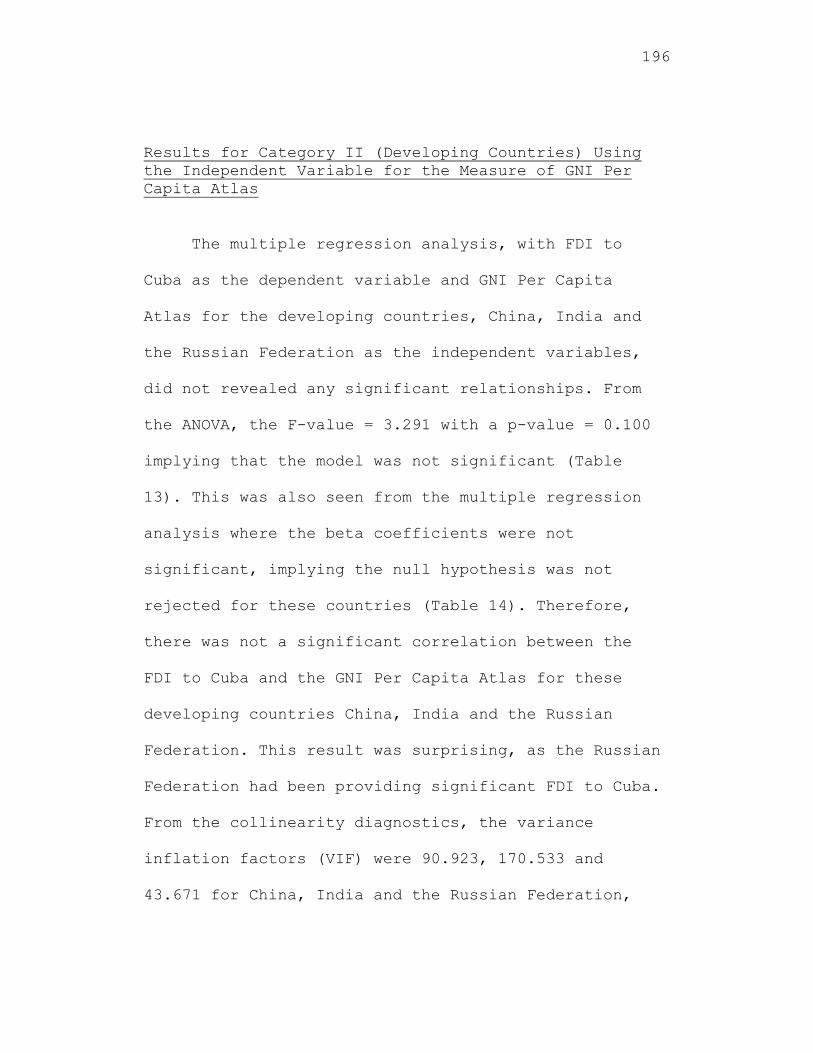
196

Results for Category II (Developing Countries) Using the Independent Variable for the Measure of GNI Per Capita Atlas

The multiple regression analysis, with FDI to

Cuba as the dependent variable and GNI Per Capita

Atlas for the developing countries, China, India and

the Russian Federation as the independent variables,

did not revealed any significant relationships. From

the ANOVA, the F-value = 3.291 with a p-value = 0.100

implying that the model was not significant (Table

13). This was also seen from the multiple regression

analysis where the beta coefficients were not

significant, implying the null hypothesis was not

rejected for these countries (Table 14). Therefore,

there was not a significant correlation between the

FDI to Cuba and the GNI Per Capita Atlas for these

developing countries China, India and the Russian

Federation. This result was surprising, as the Russian

Federation had been providing significant FDI to Cuba.

From the collinearity diagnostics, the variance

inflation factors (VIF) were 90.923, 170.533 and

43.671 for China, India and the Russian Federation,

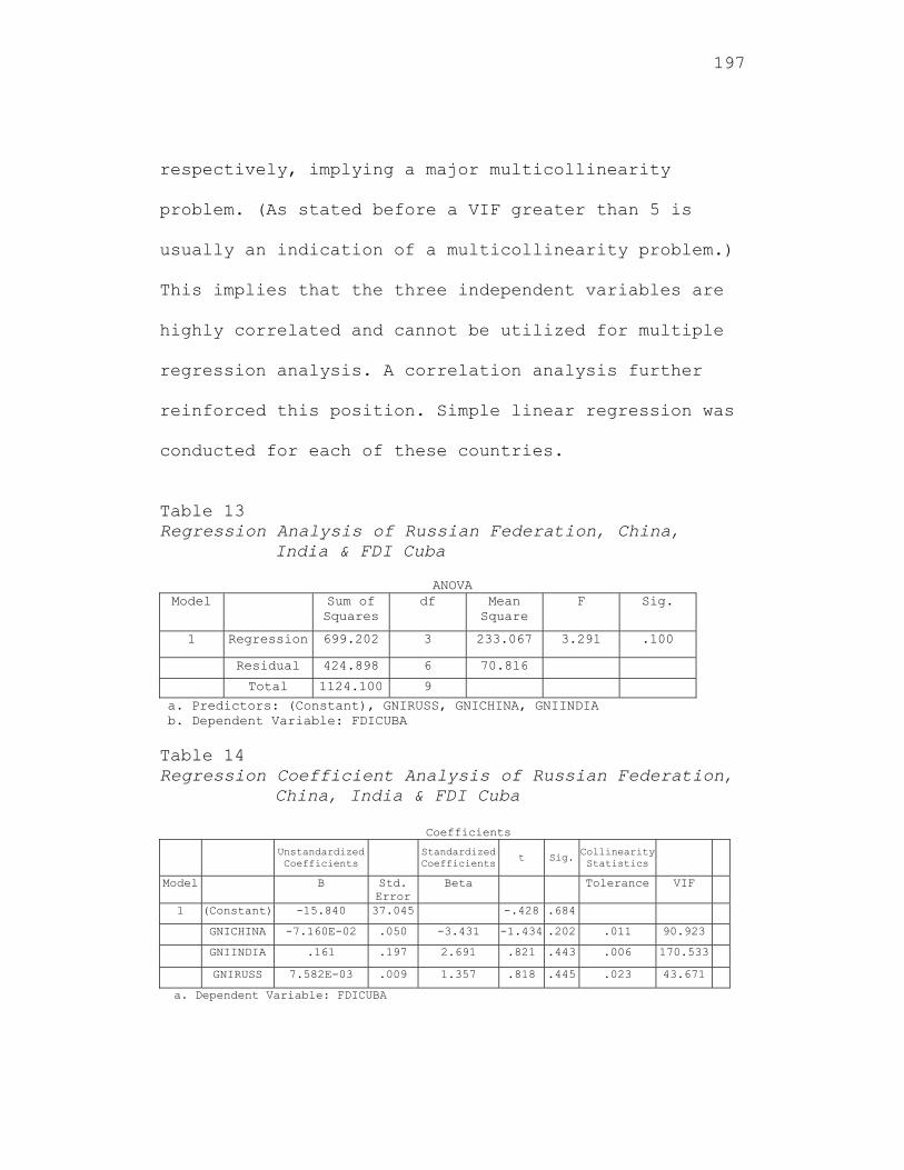
197

respectively, implying a major multicollinearity

problem. (As stated before a VIF greater than 5 is

usually an indication of a multicollinearity problem.)

This implies that the three independent variables are

highly correlated and cannot be utilized for multiple

regression analysis. A correlation analysis further

reinforced this position. Simple linear regression was

conducted for each of these countries.

Table 13 Regression Analysis of Russian Federation, China,

India & FDI Cuba

ANOVA Model Sum of

Squares df Mean

Square F Sig.

1 Regression 699.202 3 233.067 3.291 .100

Residual 424.898 6 70.816

Total 1124.100 9

a. Predictors: (Constant), GNIRUSS, GNICHINA, GNIINDIA b. Dependent Variable: FDICUBA Table 14 Regression Coefficient Analysis of Russian Federation,

China, India & FDI Cuba

Coefficients Unstandardized

Coefficients Standardized Coefficients t Sig. Collinearity

Statistics

Model B Std. Error

Beta Tolerance VIF

1 (Constant) -15.840 37.045 -.428 .684

GNICHINA -7.160E-02 .050 -3.431 -1.434 .202 .011 90.923

GNIINDIA .161 .197 2.691 .821 .443 .006 170.533

GNIRUSS 7.582E-03 .009 1.357 .818 .445 .023 43.671

a. Dependent Variable: FDICUBA

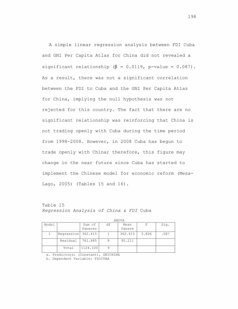
198

A simple linear regression analysis between FDI Cuba

and GNI Per Capita Atlas for China did not revealed a

significant relationship ( = 0.0119, p-value = 0.087).

As a result, there was not a significant correlation

between the FDI to Cuba and the GNI Per Capita Atlas

for China, implying the null hypothesis was not

rejected for this country. The fact that there are no

significant relationship was reinforcing that China is

not trading openly with Cuba during the time period

from 1998-2008. However, in 2008 Cuba has begun to

trade openly with China; therefore, this figure may

change in the near future since Cuba has started to

implement the Chinese model for economic reform (Mesa-

Lago, 2005) (Tables 15 and 16).

Table 15 Regression Analysis of China & FDI Cuba

ANOVA Model Sum of

Squaresdf Mean

Square F Sig.

1 Regression 362.415 1 362.415 3.806 .087

Residual 761.685 8 95.211

Total 1124.100 9

a. Predictors: (Constant), GNICHINA b. Dependent Variable: FDICUBA

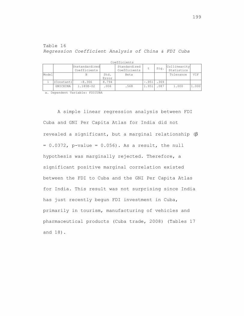
199

Table 16 Regression Coefficient Analysis of China & FDI Cuba

Coefficients Unstandardized

Coefficients Standardized

Coefficients t Sig. Collinearity

Statistics

Model B Std. Error

Beta Tolerance VIF

1 (Constant) -8.366 8.794 -.951 .369 GNICHINA 1.185E-02 .006 .568 1.951 .087 1.000 1.000

a. Dependent Variable: FDICUBA

A simple linear regression analysis between FDI

Cuba and GNI Per Capita Atlas for India did not

revealed a significant, but a marginal relationship (

= 0.0372, p-value = 0.056). As a result, the null

hypothesis was marginally rejected. Therefore, a

significant positive marginal correlation existed

between the FDI to Cuba and the GNI Per Capita Atlas

for India. This result was not surprising since India

has just recently begun FDI investment in Cuba,

primarily in tourism, manufacturing of vehicles and

pharmaceutical products (Cuba trade, 2008) (Tables 17

and 18).

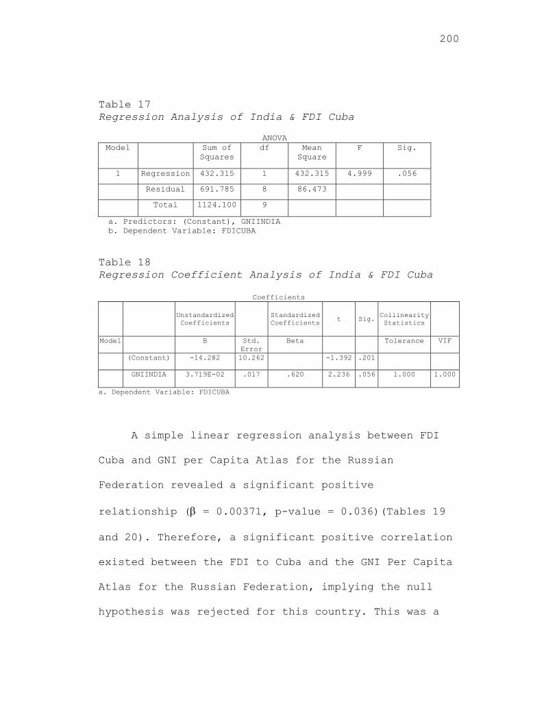
200

Table 17 Regression Analysis of India & FDI Cuba

ANOVA Model Sum of

Squares df Mean

Square F Sig.

1 Regression 432.315 1 432.315 4.999 .056

Residual 691.785 8 86.473

Total 1124.100 9

a. Predictors: (Constant), GNIINDIA b. Dependent Variable: FDICUBA Table 18 Regression Coefficient Analysis of India & FDI Cuba

Coefficients

Unstandardized Coefficients

Standardized Coefficients

t Sig.Collinearity Statistics

Model B Std. Error

Beta Tolerance VIF

(Constant) -14.282 10.262 -1.392 .201

GNIINDIA 3.719E-02 .017 .620 2.236 .056 1.000 1.000

a. Dependent Variable: FDICUBA

A simple linear regression analysis between FDI

Cuba and GNI per Capita Atlas for the Russian

Federation revealed a significant positive

relationship ( = 0.00371, p-value = 0.036)(Tables 19

and 20). Therefore, a significant positive correlation

existed between the FDI to Cuba and the GNI Per Capita

Atlas for the Russian Federation, implying the null

hypothesis was rejected for this country. This was a

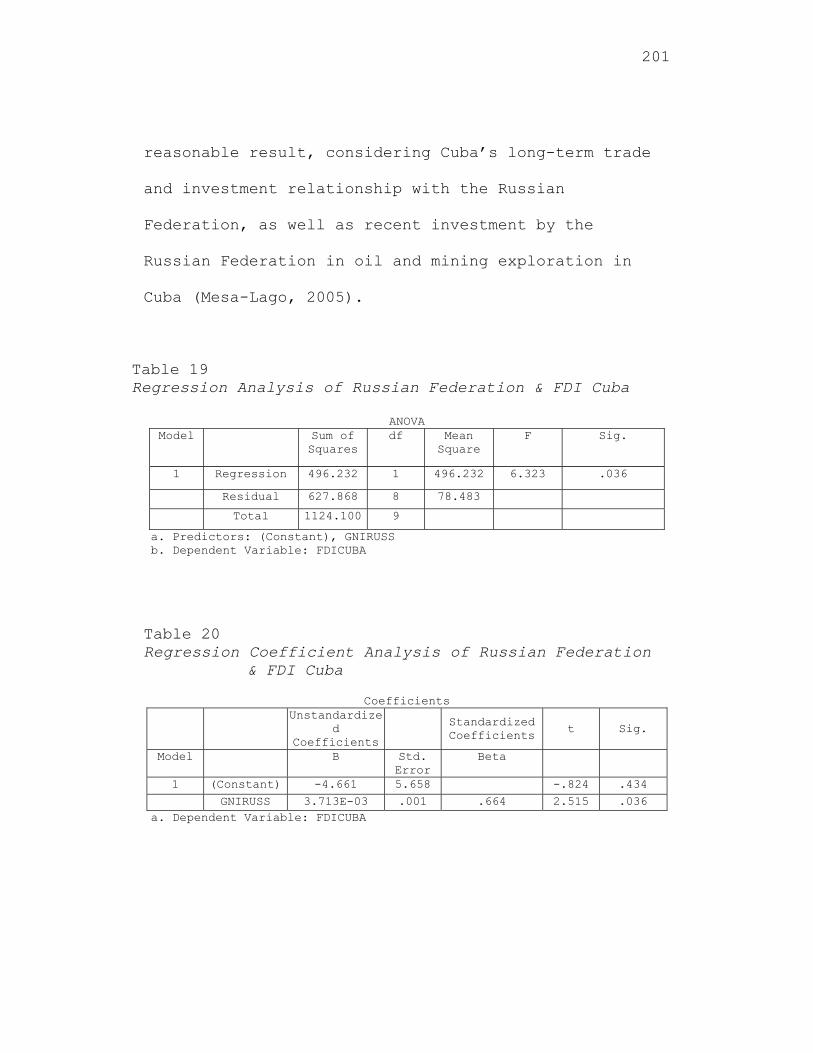
201

reasonable result, considering Cuba’s long-term trade

and investment relationship with the Russian

Federation, as well as recent investment by the

Russian Federation in oil and mining exploration in

Cuba (Mesa-Lago, 2005).

Table 19 Regression Analysis of Russian Federation & FDI Cuba

ANOVA Model Sum of

Squares df Mean

Square F Sig.

1 Regression 496.232 1 496.232 6.323 .036

Residual 627.868 8 78.483

Total 1124.100 9

a. Predictors: (Constant), GNIRUSS b. Dependent Variable: FDICUBA

Table 20 Regression Coefficient Analysis of Russian Federation

& FDI Cuba

Coefficients Unstandardize

d Coefficients

Standardized Coefficients

t Sig.

Model B Std. Error

Beta

1 (Constant) -4.661 5.658 -.824 .434

GNIRUSS 3.713E-03 .001 .664 2.515 .036 a. Dependent Variable: FDICUBA

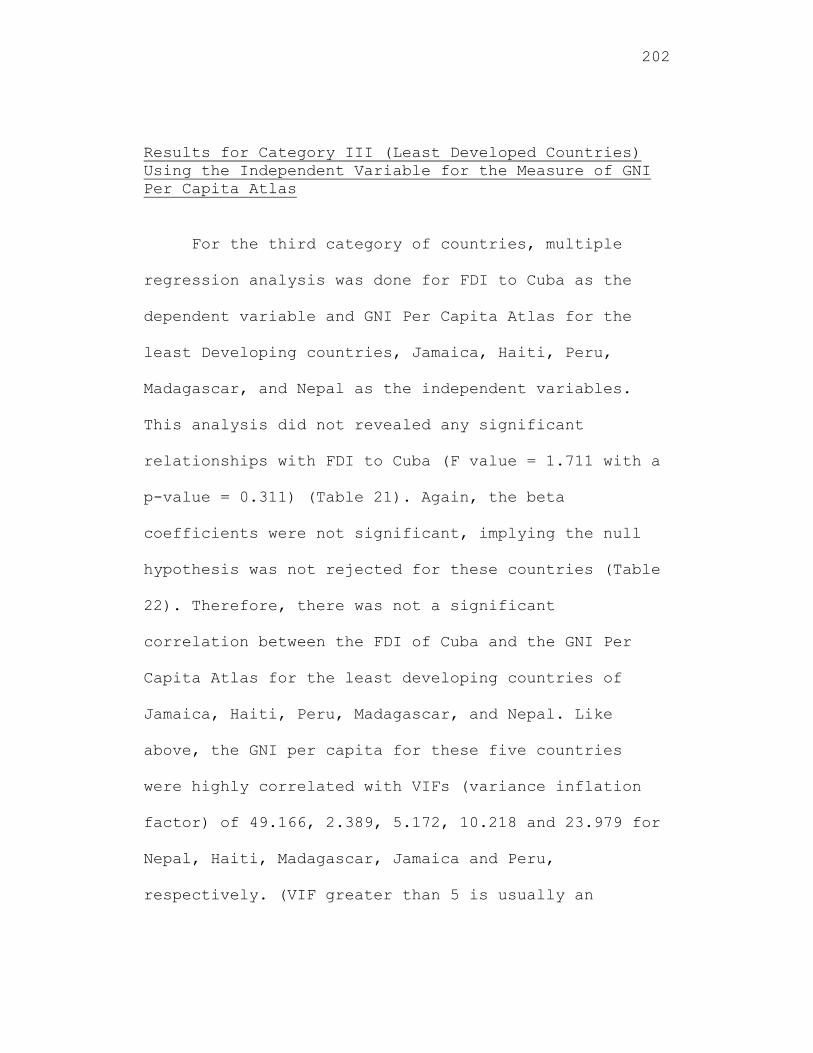
202

Results for Category III (Least Developed Countries) Using the Independent Variable for the Measure of GNI Per Capita Atlas

For the third category of countries, multiple

regression analysis was done for FDI to Cuba as the

dependent variable and GNI Per Capita Atlas for the

least Developing countries, Jamaica, Haiti, Peru,

Madagascar, and Nepal as the independent variables.

This analysis did not revealed any significant

relationships with FDI to Cuba (F value = 1.711 with a

p-value = 0.311) (Table 21). Again, the beta

coefficients were not significant, implying the null

hypothesis was not rejected for these countries (Table

22). Therefore, there was not a significant

correlation between the FDI of Cuba and the GNI Per

Capita Atlas for the least developing countries of

Jamaica, Haiti, Peru, Madagascar, and Nepal. Like

above, the GNI per capita for these five countries

were highly correlated with VIFs (variance inflation

factor) of 49.166, 2.389, 5.172, 10.218 and 23.979 for

Nepal, Haiti, Madagascar, Jamaica and Peru,

respectively. (VIF greater than 5 is usually an

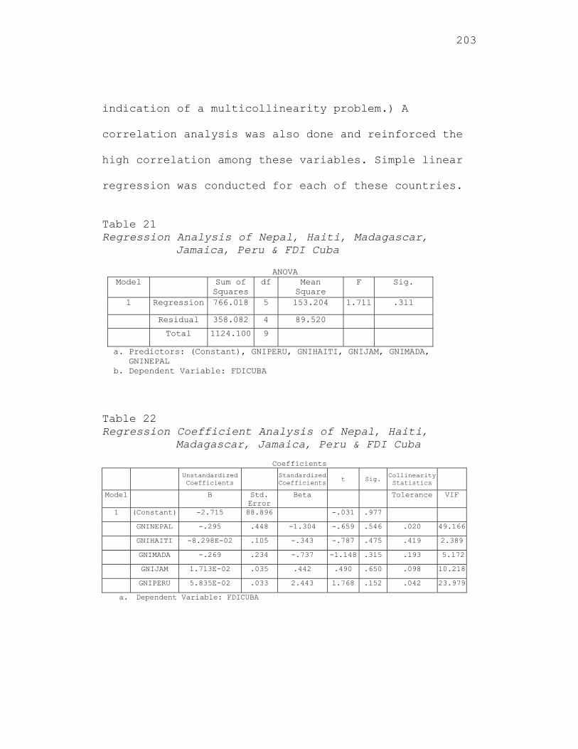
203

indication of a multicollinearity problem.) A

correlation analysis was also done and reinforced the

high correlation among these variables. Simple linear

regression was conducted for each of these countries.

Table 21 Regression Analysis of Nepal, Haiti, Madagascar,

Jamaica, Peru & FDI Cuba

ANOVA Model Sum of

Squares df Mean

Square F Sig.

1 Regression 766.018 5 153.204 1.711 .311

Residual 358.082 4 89.520

Total 1124.100 9

a. Predictors: (Constant), GNIPERU, GNIHAITI, GNIJAM, GNIMADA, GNINEPAL b. Dependent Variable: FDICUBA

Table 22 Regression Coefficient Analysis of Nepal, Haiti,

Madagascar, Jamaica, Peru & FDI Cuba Coefficients

Unstandardized Coefficients Standardized

Coefficients t Sig. Collinearity Statistics

Model B Std. Error

Beta Tolerance VIF

1 (Constant) -2.715 88.896 -.031 .977

GNINEPAL -.295 .448 -1.304 -.659 .546 .020 49.166

GNIHAITI -8.298E-02 .105 -.343 -.787 .475 .419 2.389

GNIMADA -.269 .234 -.737 -1.148 .315 .193 5.172

GNIJAM 1.713E-02 .035 .442 .490 .650 .098 10.218

GNIPERU 5.835E-02 .033 2.443 1.768 .152 .042 23.979

a. Dependent Variable: FDICUBA

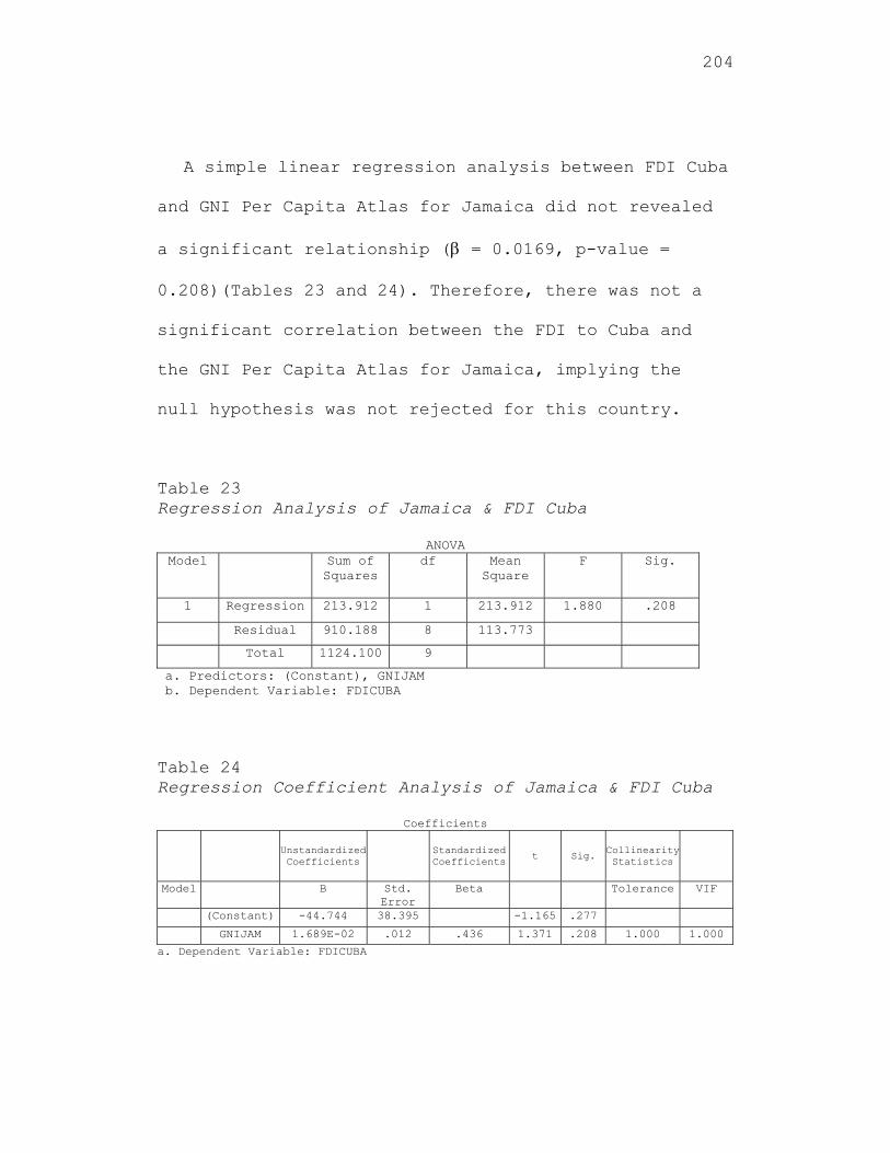
204

A simple linear regression analysis between FDI Cuba

and GNI Per Capita Atlas for Jamaica did not revealed

a significant relationship ( = 0.0169, p-value =

0.208)(Tables 23 and 24). Therefore, there was not a

significant correlation between the FDI to Cuba and

the GNI Per Capita Atlas for Jamaica, implying the

null hypothesis was not rejected for this country.

Table 23 Regression Analysis of Jamaica & FDI Cuba

ANOVA Model Sum of

Squares df Mean

Square F Sig.

1 Regression 213.912 1 213.912 1.880 .208

Residual 910.188 8 113.773

Total 1124.100 9

a. Predictors: (Constant), GNIJAM b. Dependent Variable: FDICUBA Table 24 Regression Coefficient Analysis of Jamaica & FDI Cuba

Coefficients

Unstandardized Coefficients Standardized

Coefficients t Sig. Collinearity Statistics

Model B Std. Error

Beta Tolerance VIF

(Constant) -44.744 38.395 -1.165 .277

GNIJAM 1.689E-02 .012 .436 1.371 .208 1.000 1.000

a. Dependent Variable: FDICUBA

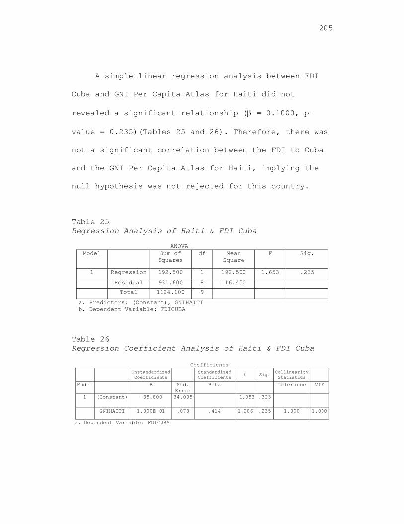
205

A simple linear regression analysis between FDI

Cuba and GNI Per Capita Atlas for Haiti did not

revealed a significant relationship ( = 0.1000, p-

value = 0.235)(Tables 25 and 26). Therefore, there was

not a significant correlation between the FDI to Cuba

and the GNI Per Capita Atlas for Haiti, implying the

null hypothesis was not rejected for this country.

Table 25 Regression Analysis of Haiti & FDI Cuba

ANOVA Model Sum of

Squares df Mean

Square F Sig.

1 Regression 192.500 1 192.500 1.653 .235

Residual 931.600 8 116.450

Total 1124.100 9

a. Predictors: (Constant), GNIHAITI b. Dependent Variable: FDICUBA Table 26 Regression Coefficient Analysis of Haiti & FDI Cuba

Coefficients Unstandardized

Coefficients Standardized Coefficients t Sig. Collinearity

Statistics

Model B Std. Error

Beta Tolerance VIF

1 (Constant) -35.800 34.005 -1.053 .323

GNIHAITI 1.000E-01 .078 .414 1.286 .235 1.000 1.000

a. Dependent Variable: FDICUBA

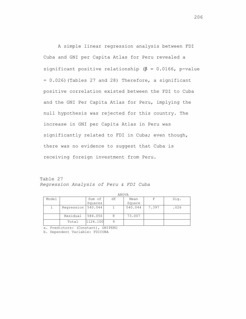
206

A simple linear regression analysis between FDI

Cuba and GNI per Capita Atlas for Peru revealed a

significant positive relationship ( = 0.0166, p-value

= 0.026)(Tables 27 and 28) Therefore, a significant

positive correlation existed between the FDI to Cuba

and the GNI Per Capita Atlas for Peru, implying the

null hypothesis was rejected for this country. The

increase in GNI per Capita Atlas in Peru was

significantly related to FDI in Cuba; even though,

there was no evidence to suggest that Cuba is

receiving foreign investment from Peru.

Table 27 Regression Analysis of Peru & FDI Cuba

ANOVA Model Sum of

Squaresdf Mean

Square F Sig.

1 Regression 540.044 1 540.044 7.397 .026

Residual 584.056 8 73.007

Total 1124.100 9

a. Predictors: (Constant), GNIPERU b. Dependent Variable: FDICUBA

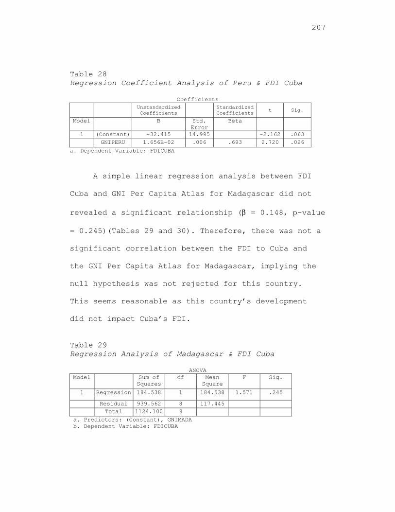
207

Table 28 Regression Coefficient Analysis of Peru & FDI Cuba

Coefficients Unstandardized

Coefficients Standardized

Coefficientst Sig.

Model B Std. Error

Beta

1 (Constant) -32.415 14.995 -2.162 .063 GNIPERU 1.656E-02 .006 .693 2.720 .026

a. Dependent Variable: FDICUBA

A simple linear regression analysis between FDI

Cuba and GNI Per Capita Atlas for Madagascar did not

revealed a significant relationship ( = 0.148, p-value

= 0.245)(Tables 29 and 30). Therefore, there was not a

significant correlation between the FDI to Cuba and

the GNI Per Capita Atlas for Madagascar, implying the

null hypothesis was not rejected for this country.

This seems reasonable as this country’s development

did not impact Cuba’s FDI.

Table 29 Regression Analysis of Madagascar & FDI Cuba

ANOVA Model Sum of

Squares df Mean

Square F Sig.

1 Regression 184.538 1 184.538 1.571 .245

Residual 939.562 8 117.445 Total 1124.100 9

a. Predictors: (Constant), GNIMADA b. Dependent Variable: FDICUBA

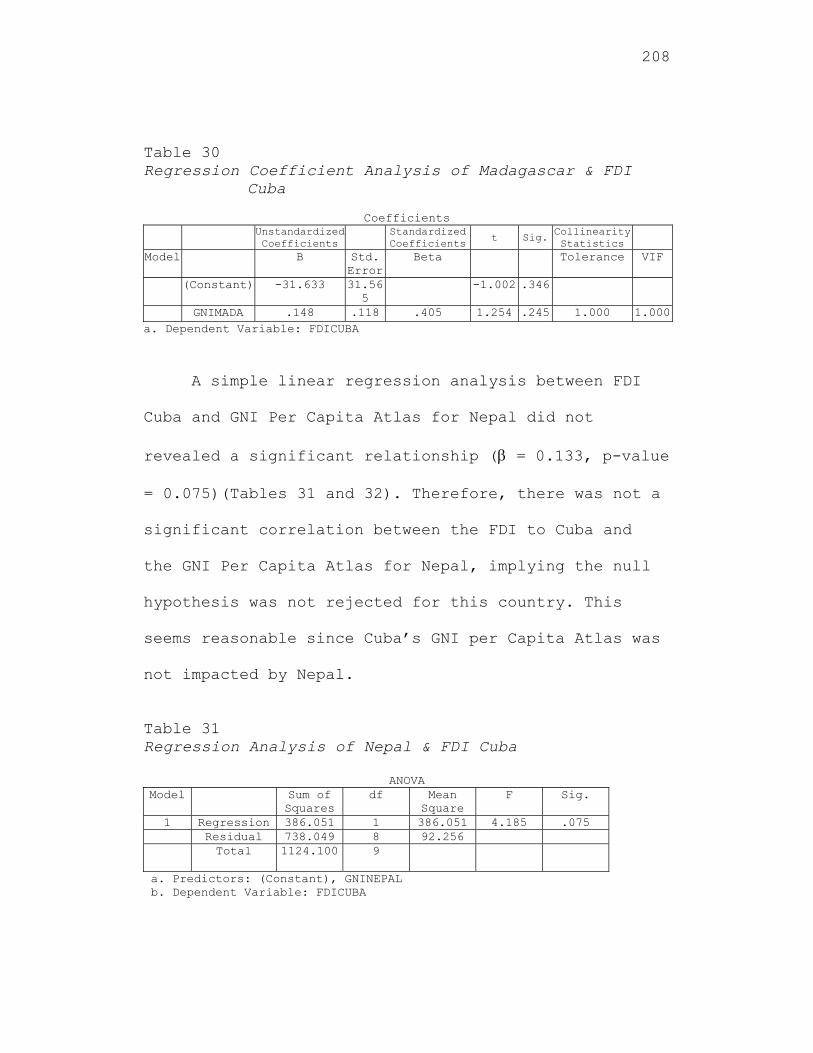
208

Table 30 Regression Coefficient Analysis of Madagascar & FDI

Cuba

Coefficients Unstandardized

Coefficients Standardized

Coefficientst Sig. Collinearity

Statistics

Model B Std. Error

Beta Tolerance VIF

(Constant) -31.633 31.565

-1.002 .346

GNIMADA .148 .118 .405 1.254 .245 1.000 1.000a. Dependent Variable: FDICUBA

A simple linear regression analysis between FDI

Cuba and GNI Per Capita Atlas for Nepal did not

revealed a significant relationship ( = 0.133, p-value

= 0.075)(Tables 31 and 32). Therefore, there was not a

significant correlation between the FDI to Cuba and

the GNI Per Capita Atlas for Nepal, implying the null

hypothesis was not rejected for this country. This

seems reasonable since Cuba’s GNI per Capita Atlas was

not impacted by Nepal.

Table 31 Regression Analysis of Nepal & FDI Cuba

ANOVA Model Sum of

Squares df Mean

Square F Sig.

1 Regression 386.051 1 386.051 4.185 .075 Residual 738.049 8 92.256 Total 1124.100 9

a. Predictors: (Constant), GNINEPAL b. Dependent Variable: FDICUBA

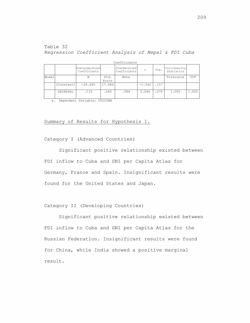
209

Table 32 Regression Coefficient Analysis of Nepal & FDI Cuba

Coefficients

Unstandardized Coefficients Standardized

Coefficients t Sig. Collinearity Statistics

Model B Std. Error

Beta Tolerance VIF

(Constant) -26.695 17.086 -1.562 .157

GNINEPAL .133 .065 .586 2.046 .075 1.000 1.000

a. Dependent Variable: FDICUBA

Summary of Results for Hypothesis 1.

Category I (Advanced Countries)

Significant positive relationship existed between

FDI inflow to Cuba and GNI per Capita Atlas for

Germany, France and Spain. Insignificant results were

found for the United States and Japan.

Category II (Developing Countries)

Significant positive relationship existed between

FDI inflow to Cuba and GNI per Capita Atlas for the

Russian Federation. Insignificant results were found

for China, while India showed a positive marginal

result.

210

Category III (Least Developing Countries)

Significant positive relationship existed between

FDI inflow to Cuba and GNI per Capita Atlas for Peru.

Insignificant results were found for Jamaica, Haiti,

Madagascar and Nepal.

Results for Hypothesis 2

FDI to Cuba was the dependent variable. For the

advanced countries, the independent variables were the

Financial Capital for the United States, Japan,

Germany, France and Spain (Sawalha, 2007). The

independent variables for the developing countries

were Financial Capital for China, India and the

Russian Federation (Sawalha, 2007). The independent

variables for the Least Developed Countries (LCD’s)

were Financial Capital for Jamaica, Haiti, Peru,

Madagascar and Nepal. The Republic of Cuba’s Financial

Capital was not included in the model as there were

only three data points. Proxies for financial capital

included two variables, Gross Fixed Capital Formation

211

(percent annual growth of GDP) and Gross Capital

Formation (percent of GDP).

The second hypothesis to be tested is:

Hypothesis H02: The level of contribution of FDI

inflow to Cuba is not significantly related to

the Financial Capital for the three groups of

countries.

Hypothesis HA2: The level of contribution of FDI

inflow to Cuba is significantly related to the

Financial Capital for three groups of

countries.

The multiple regression models to test Hypothesis 2

are listed below.

Category I (Advanced Countries)

FDICUBA = αO + α1FCPCAPUS + α2FCPCAPJapan + α3FCPCAPGermany +

α4FCPCAPFrance + α5FCPCAPSpain + ε1

212

Categories II (Developing Countries)

FDICUBA = O + 1FCPCAPChina + 2FCPCAPIndia + 3FCPCAPRussian

Federation +ε2

Categories III (Least Developed Countries)

FDICUBA = δ + δ1FCPCAPJamaica + δ2FCPCAPHaiti + δ3FCPCAPPeru +

δ4FCPCAPMadagascar + δ5FCPCAPNepal + ε3

The results was presented for both independent

variables measuring gross fixed capital and gross

capital formation for each of the three categories of

countries.

Results for Gross Fixed Capital Formation

Pearson Correlation Analysis

A Pearson Correlation Analysis among the

advanced, developing, and least developed non-oil

producing countries revealed a significant correlation

between FDI for Cuba and Gross Fixed Capital Formation

(percent annual growth of GDP) for India (Table 33).

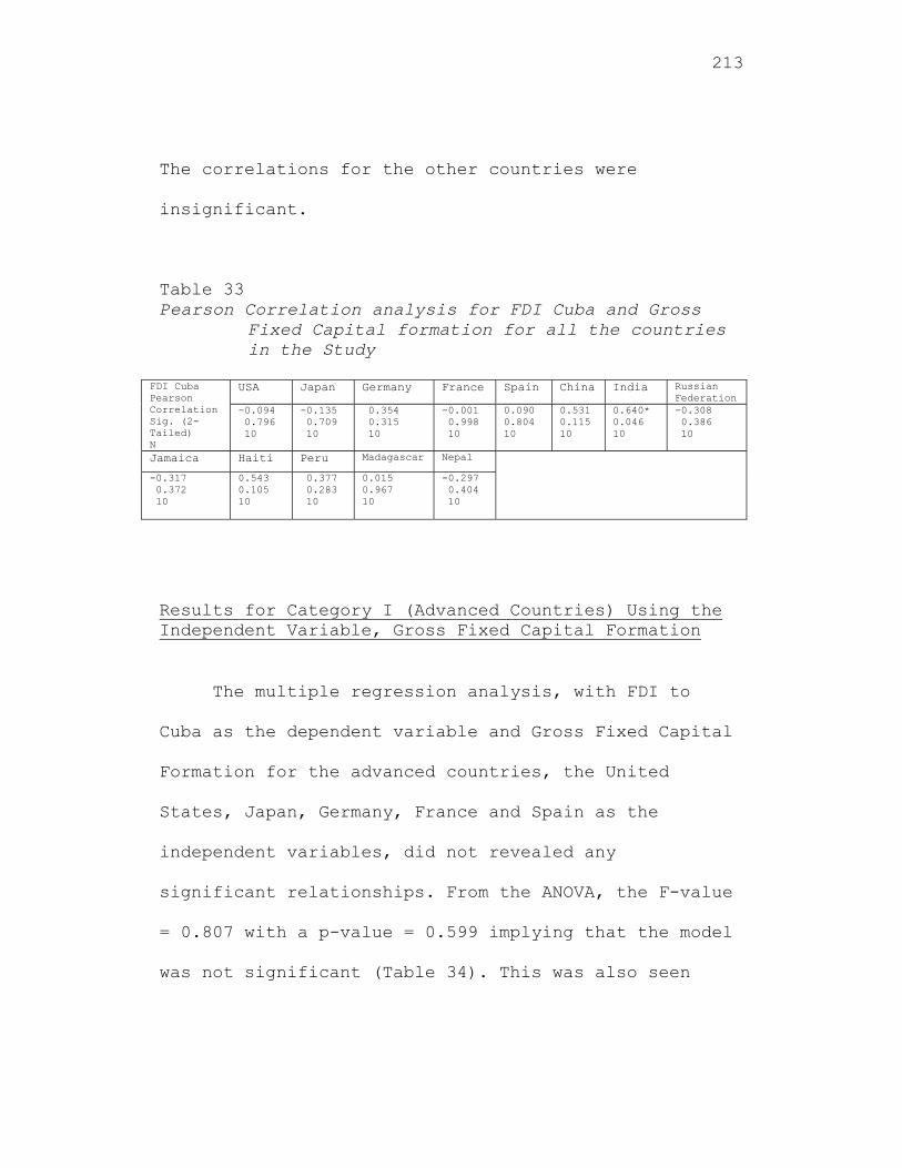
213

The correlations for the other countries were

insignificant.

Table 33 Pearson Correlation analysis for FDI Cuba and Gross

Fixed Capital formation for all the countries in the Study

FDI Cuba Pearson Correlation Sig. (2-Tailed) N

USA Japan Germany France Spain China India Russian Federation

-0.094 0.796 10

-0.135 0.709 10

0.354 0.315 10

-0.001 0.998 10

0.090 0.804 10

0.531 0.115 10

0.640* 0.046 10

-0.308 0.386 10

Jamaica Haiti Peru Madagascar Nepal

-0.317 0.372 10

0.543 0.105 10

0.377 0.283 10

0.015 0.967 10

-0.297 0.404 10

Results for Category I (Advanced Countries) Using the Independent Variable, Gross Fixed Capital Formation

The multiple regression analysis, with FDI to

Cuba as the dependent variable and Gross Fixed Capital

Formation for the advanced countries, the United

States, Japan, Germany, France and Spain as the

independent variables, did not revealed any

significant relationships. From the ANOVA, the F-value

= 0.807 with a p-value = 0.599 implying that the model

was not significant (Table 34). This was also seen

214

from the multiple regression analysis where the beta

coefficients were not significant, implying the null

hypothesis was not rejected for these countries (Table

35). Therefore, there was not a significant

correlation between the FDI to Cuba and the Gross

Fixed Capital Formation for these advanced countries,

the United States, Japan, Germany, France and Spain.

This result was surprising as Germany, France and

Spain had been providing significant FDI to Cuba. From

the collinearity diagnostics, the variance inflation

factor (VIF) was 2.005, 1.578, 3.611, 5.414 and 3.356

for the United States, Japan, Germany, France and

Spain, respectively, implying a multicollinearity

problem. (VIF greater than 5 is usually an indication

of a multicollinearity problem.) This implied that one

of the five independent variables was highly

correlated with one or more of the other four

independent variables. A correlation analysis further

reinforced this position. Simple linear regression was

conducted for each of these countries.

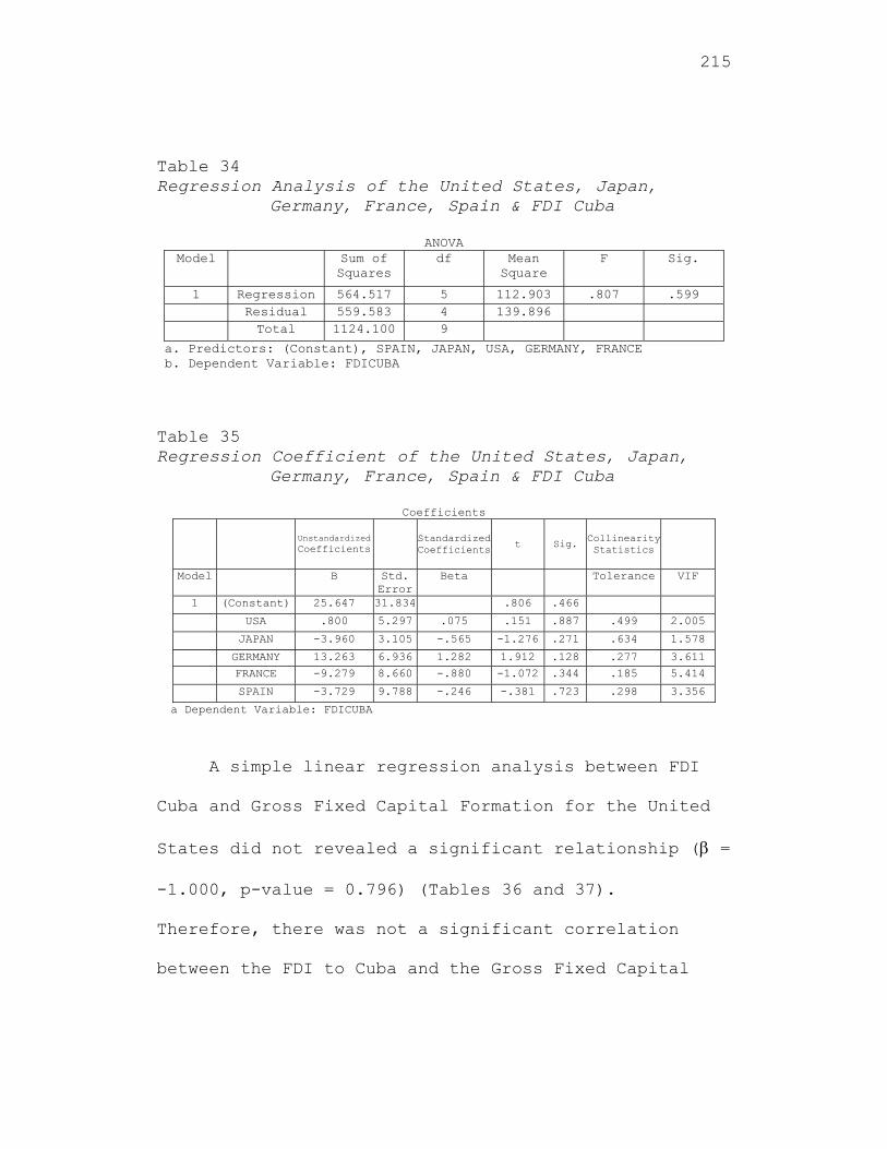
215

Table 34 Regression Analysis of the United States, Japan,

Germany, France, Spain & FDI Cuba

ANOVA Model Sum of

Squares df Mean

Square F Sig.

1 Regression 564.517 5 112.903 .807 .599 Residual 559.583 4 139.896 Total 1124.100 9

a. Predictors: (Constant), SPAIN, JAPAN, USA, GERMANY, FRANCE b. Dependent Variable: FDICUBA Table 35 Regression Coefficient of the United States, Japan,

Germany, France, Spain & FDI Cuba

Coefficients

Unstandardized Coefficients Standardized

Coefficients t Sig. Collinearity Statistics

Model B Std. Error

Beta Tolerance VIF

1 (Constant) 25.647 31.834 .806 .466

USA .800 5.297 .075 .151 .887 .499 2.005

JAPAN -3.960 3.105 -.565 -1.276 .271 .634 1.578

GERMANY 13.263 6.936 1.282 1.912 .128 .277 3.611

FRANCE -9.279 8.660 -.880 -1.072 .344 .185 5.414

SPAIN -3.729 9.788 -.246 -.381 .723 .298 3.356

a Dependent Variable: FDICUBA

A simple linear regression analysis between FDI

Cuba and Gross Fixed Capital Formation for the United

States did not revealed a significant relationship ( =

-1.000, p-value = 0.796) (Tables 36 and 37).

Therefore, there was not a significant correlation

between the FDI to Cuba and the Gross Fixed Capital

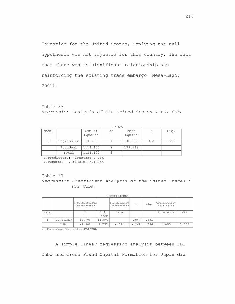
216

Formation for the United States, implying the null

hypothesis was not rejected for this country. The fact

that there was no significant relationship was

reinforcing the existing trade embargo (Mesa-Lago,

2001).

Table 36 Regression Analysis of the United States & FDI Cuba

ANOVA Model Sum of

Squares df Mean

Square F Sig.

1 Regression 10.000 1 10.000 .072 .796

Residual 1114.100 8 139.263

Total 1124.100 9

a.Predictors: (Constant), USA b.Dependent Variable: FDICUBA Table 37 Regression Coefficient Analysis of the United States &

FDI Cuba

Coefficients

Unstandardized Coefficients Standardized

Coefficients t Sig. Collinearity Statistics

Model B Std. Error

Beta Tolerance VIF

1 (Constant) 10.700 11.801 .907 .391

USA -1.000 3.732 -.094 -.268 .796 1.000 1.000

a. Dependent Variable: FDICUBA

A simple linear regression analysis between FDI

Cuba and Gross Fixed Capital Formation for Japan did

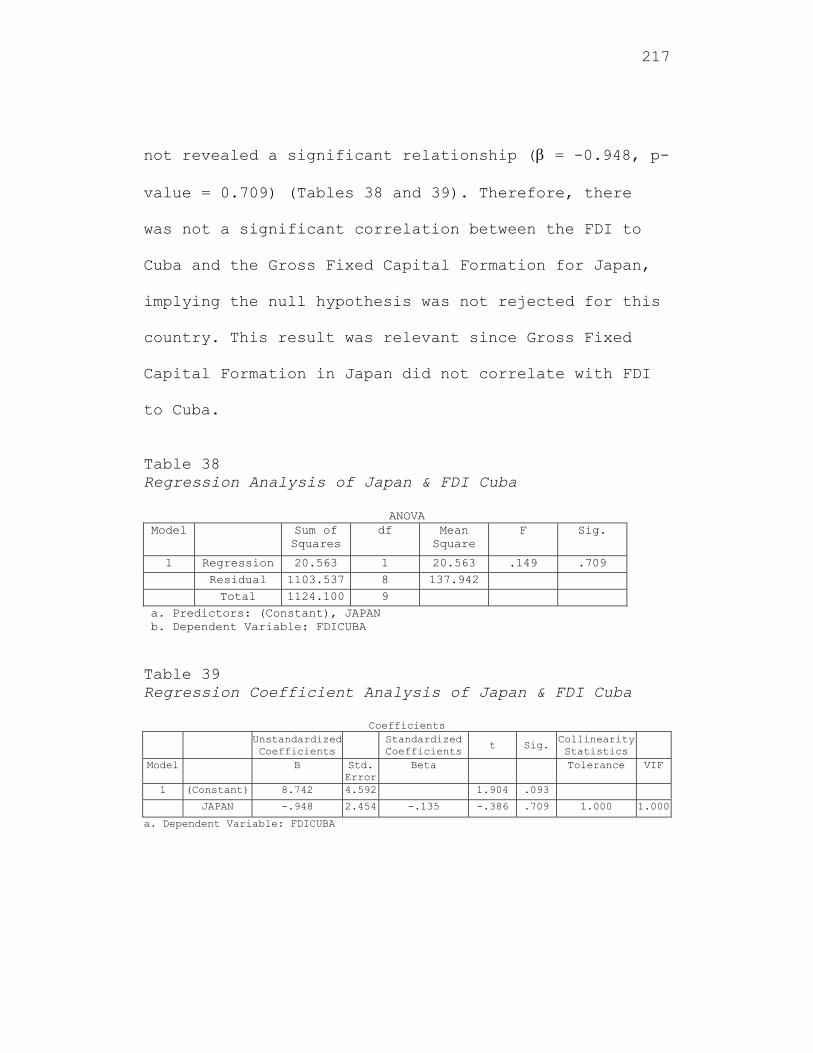
217

not revealed a significant relationship ( = -0.948, p-

value = 0.709) (Tables 38 and 39). Therefore, there

was not a significant correlation between the FDI to

Cuba and the Gross Fixed Capital Formation for Japan,

implying the null hypothesis was not rejected for this

country. This result was relevant since Gross Fixed

Capital Formation in Japan did not correlate with FDI

to Cuba.

Table 38 Regression Analysis of Japan & FDI Cuba

ANOVA Model Sum of

Squares df Mean

Square F Sig.

1 Regression 20.563 1 20.563 .149 .709 Residual 1103.537 8 137.942 Total 1124.100 9

a. Predictors: (Constant), JAPAN b. Dependent Variable: FDICUBA Table 39 Regression Coefficient Analysis of Japan & FDI Cuba

Coefficients Unstandardized

Coefficients Standardized

Coefficientst Sig. Collinearity

Statistics

Model B Std. Error

Beta Tolerance VIF

1 (Constant) 8.742 4.592 1.904 .093

JAPAN -.948 2.454 -.135 -.386 .709 1.000 1.000

a. Dependent Variable: FDICUBA

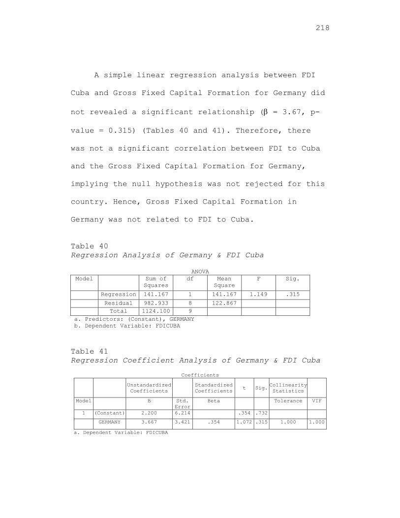
218

A simple linear regression analysis between FDI

Cuba and Gross Fixed Capital Formation for Germany did

not revealed a significant relationship ( = 3.67, p-

value = 0.315) (Tables 40 and 41). Therefore, there

was not a significant correlation between FDI to Cuba

and the Gross Fixed Capital Formation for Germany,

implying the null hypothesis was not rejected for this

country. Hence, Gross Fixed Capital Formation in

Germany was not related to FDI to Cuba.

Table 40 Regression Analysis of Germany & FDI Cuba

ANOVA Model Sum of

Squares df Mean

Square F Sig.

Regression 141.167 1 141.167 1.149 .315

Residual 982.933 8 122.867 Total 1124.100 9

a. Predictors: (Constant), GERMANY b. Dependent Variable: FDICUBA Table 41 Regression Coefficient Analysis of Germany & FDI Cuba

Coefficients

Unstandardized Coefficients

Standardized Coefficients

t Sig. Collinearity Statistics

Model B Std. Error

Beta Tolerance VIF

1 (Constant) 2.200 6.214 .354 .732

GERMANY 3.667 3.421 .354 1.072 .315 1.000 1.000

a. Dependent Variable: FDICUBA

219

A simple linear regression analysis between FDI

Cuba and Gross Fixed Capital Formation for France did

not revealed a significant relationship ( = -0.00990,

p-value = 0.998) (Tables 42 and 43). Therefore, there

was not a significant correlation between FDI to Cuba

and the Gross Fixed Capital Formation for France,

implying that the null hypothesis was not rejected for

this country. This result was relevant since Gross

Fixed Capital Formation in France did not correlate

with FDI to Cuba.

Table 42 Regression Analysis of France & FDI Cuba

ANOVA

Model Sum of Squares

df Mean Square F Sig.

1 Regression 9.901E-04 1 9.901E-04 .000 .998 Residual 1124.099 8 140.512 Total 1124.100 9

a. Predictors: (Constant), FRANCE b. Dependent Variable: FDICUBA

Table 43 Regression Coefficient Analysis of France & FDI Cuba

Coefficients

Unstandardized Coefficients

Standardized Coefficients t Sig.

Collinearity Statistics

Model B Std. Error

Beta Tolerance VIF

1 (Constant) 7.723 9.362 .825 .433

FRANCE -9.901E-03 3.730 -.001 -.003 .998 1.000 1.000

a. Dependent Variable: FDICUBA

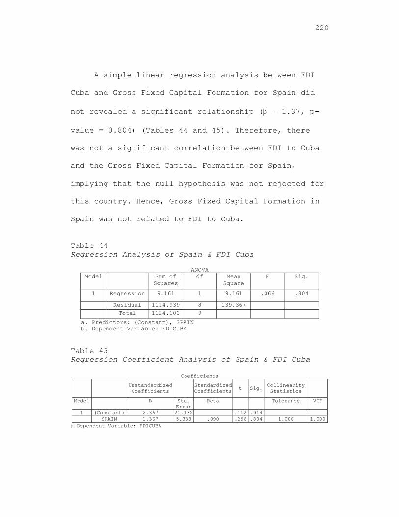
220

A simple linear regression analysis between FDI

Cuba and Gross Fixed Capital Formation for Spain did

not revealed a significant relationship ( = 1.37, p-

value = 0.804) (Tables 44 and 45). Therefore, there

was not a significant correlation between FDI to Cuba

and the Gross Fixed Capital Formation for Spain,

implying that the null hypothesis was not rejected for

this country. Hence, Gross Fixed Capital Formation in

Spain was not related to FDI to Cuba.

Table 44 Regression Analysis of Spain & FDI Cuba

ANOVA Model Sum of

Squares df Mean

Square F Sig.

1 Regression 9.161 1 9.161 .066 .804

Residual 1114.939 8 139.367 Total 1124.100 9

a. Predictors: (Constant), SPAIN b. Dependent Variable: FDICUBA Table 45 Regression Coefficient Analysis of Spain & FDI Cuba

Coefficients

Unstandardized Coefficients

Standardized Coefficients t Sig.

Collinearity Statistics

Model B Std. Error

Beta Tolerance VIF

1 (Constant) 2.367 21.132 .112 .914 SPAIN 1.367 5.333 .090 .256 .804 1.000 1.000

a Dependent Variable: FDICUBA

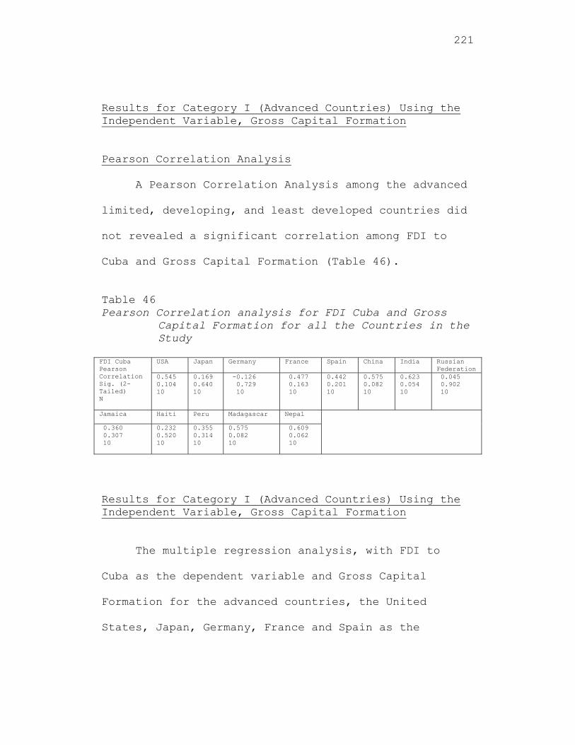
221

Results for Category I (Advanced Countries) Using the Independent Variable, Gross Capital Formation

Pearson Correlation Analysis

A Pearson Correlation Analysis among the advanced

limited, developing, and least developed countries did

not revealed a significant correlation among FDI to

Cuba and Gross Capital Formation (Table 46).

Table 46 Pearson Correlation analysis for FDI Cuba and Gross

Capital Formation for all the Countries in the Study

FDI Cuba Pearson Correlation Sig. (2-Tailed) N

USA Japan Germany France Spain China India Russian Federation

0.545 0.104 10

0.169 0.640 10

-0.126 0.729 10

0.477 0.163 10

0.442 0.201 10

0.575 0.082 10

0.623 0.054 10

0.045 0.902 10

Jamaica Haiti Peru Madagascar Nepal

0.360 0.307 10

0.232 0.520 10

0.355 0.314 10

0.575 0.082 10

0.609 0.062 10

Results for Category I (Advanced Countries) Using the Independent Variable, Gross Capital Formation

The multiple regression analysis, with FDI to

Cuba as the dependent variable and Gross Capital

Formation for the advanced countries, the United

States, Japan, Germany, France and Spain as the

222

independent variables, did not revealed any

significant relationships. From the ANOVA, the F-value

= 1.817 with a p-value = 0.291 implying that the model

was not significant (Table 47). This was also seen

from the multiple regression analysis where the beta

coefficients were not significant, implying the null

hypothesis was not rejected for these countries (Table

48). Therefore, there was not a significant

correlation between the FDI to Cuba and the Gross

Capital Formation for these advanced countries, the

United States, Japan, Germany, France and Spain. This

result is surprising as Germany, France and Spain had

been providing significant FDI to Cuba. From the

collinearity diagnostics, the variance inflation

factor (VIF) was 5.838, 10.513, 8.113, 8.273 and

21.285 for the United States, Japan, Germany, France

and Spain, respectively implying a major

multicollinearity problem (A VIF greater than 5 is

usually an indication of a multicollinearity problem.)

This implies that all the independent variables are

highly correlated and cannot be utilized for multiple

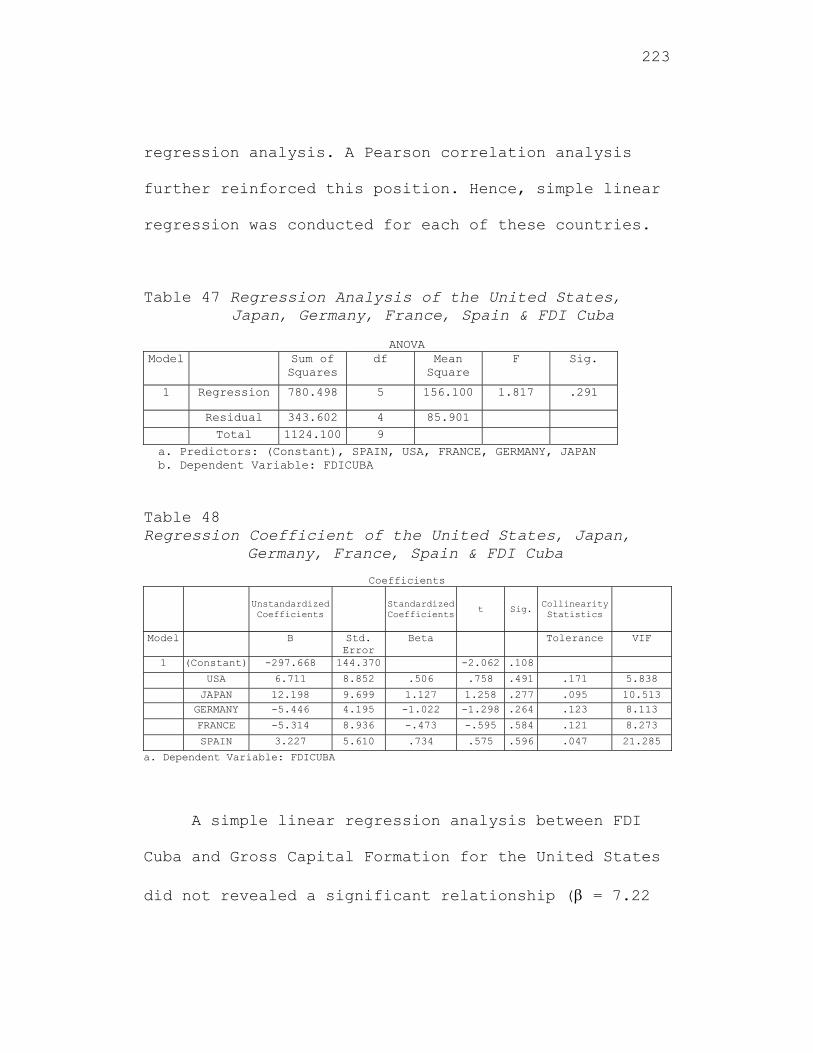
223

regression analysis. A Pearson correlation analysis

further reinforced this position. Hence, simple linear

regression was conducted for each of these countries.

Table 47 Regression Analysis of the United States,

Japan, Germany, France, Spain & FDI Cuba

ANOVA Model Sum of

Squares df Mean

Square F Sig.

1 Regression 780.498 5 156.100 1.817 .291

Residual 343.602 4 85.901

Total 1124.100 9

a. Predictors: (Constant), SPAIN, USA, FRANCE, GERMANY, JAPAN b. Dependent Variable: FDICUBA

Table 48 Regression Coefficient of the United States, Japan,

Germany, France, Spain & FDI Cuba

Coefficients

Unstandardized Coefficients Standardized

Coefficients t Sig. Collinearity Statistics

Model B Std. Error

Beta Tolerance VIF

1 (Constant) -297.668 144.370 -2.062 .108

USA 6.711 8.852 .506 .758 .491 .171 5.838

JAPAN 12.198 9.699 1.127 1.258 .277 .095 10.513 GERMANY -5.446 4.195 -1.022 -1.298 .264 .123 8.113

FRANCE -5.314 8.936 -.473 -.595 .584 .121 8.273

SPAIN 3.227 5.610 .734 .575 .596 .047 21.285

a. Dependent Variable: FDICUBA

A simple linear regression analysis between FDI

Cuba and Gross Capital Formation for the United States

did not revealed a significant relationship ( = 7.22

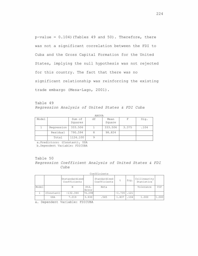
224

p-value = 0.104)(Tables 49 and 50). Therefore, there

was not a significant correlation between the FDI to

Cuba and the Gross Capital Formation for the United

States, implying the null hypothesis was not rejected

for this country. The fact that there was no

significant relationship was reinforcing the existing

trade embargo (Mesa-Lago, 2001).

Table 49 Regression Analysis of United States & FDI Cuba

ANOVA Model Sum of

Squares df Mean

Square F Sig.

1 Regression 333.506 1 333.506 3.375 .104

Residual 790.594 8 98.824

Total 1124.100 9

a.Predictors: (Constant), USA b.Dependent Variable: FDICUBA

Table 50 Regression Coefficient Analysis of United States & FDI

Cuba

Coefficients

Unstandardized Coefficients

Standardized Coefficients

t Sig. Collinearity Statistics

Model B Std. Error

Beta Tolerance VIF

1 (Constant) -132.344 76.298 -1.735 .121

USA 7.219 3.930 .545 1.837 .104 1.000 1.000

a. Dependent Variable: FDICUBA

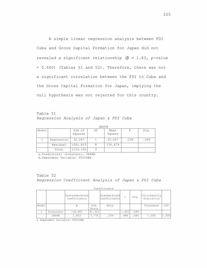
225

A simple linear regression analysis between FDI

Cuba and Gross Capital Formation for Japan did not

revealed a significant relationship ( = 1.83, p-value

= 0.640) (Tables 51 and 52). Therefore, there was not

a significant correlation between the FDI to Cuba and

the Gross Capital Formation for Japan, implying the

null hypothesis was not rejected for this country.

Table 51 Regression Analysis of Japan & FDI Cuba

ANOVA Model Sum of

Squares df Mean

Square F Sig.

1 Regression 32.267 1 32.267 .236 .640

Residual 1091.833 8 136.479

Total 1124.100 9

a.Predictors: (Constant), JAPAN b.Dependent Variable: FDICUBA

Table 52 Regression Coefficient Analysis of Japan & FDI Cuba

Coefficients

Unstandardized Coefficients

Standardized Coefficients

t Sig. Collinearity Statistics

Model B Std. Error

Beta Tolerance VIF

1 (Constant) -36.667 91.321 -.402 .699 JAPAN 1.833 3.770 .169 .486 .640 1.000 1.000

a Dependent Variable: FDICUBA

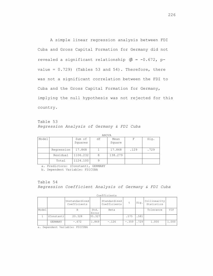
226

A simple linear regression analysis between FDI

Cuba and Gross Capital Formation for Germany did not

revealed a significant relationship ( = -0.672, p-

value = 0.729) (Tables 53 and 54). Therefore, there

was not a significant correlation between the FDI to

Cuba and the Gross Capital Formation for Germany,

implying the null hypothesis was not rejected for this

country.

Table 53 Regression Analysis of Germany & FDI Cuba

ANOVA Model Sum of

Squares df Mean

Square F Sig.

Regression 17.868 1 17.868 .129 .729

Residual 1106.232 8 138.279

Total 1124.100 9

a. Predictors: (Constant), GERMANY b. Dependent Variable: FDICUBA Table 54 Regression Coefficient Analysis of Germany & FDI Cuba

Coefficients

Unstandardized Coefficients

Standardized Coefficients t Sig.

Collinearity Statistics

Model B Std. Error

Beta Tolerance VIF

1 (Constant) 20.328 35.327 .575 .581

GERMANY -.672 1.869 -.126 -.359 .729 1.000 1.000

a. Dependent Variable: FDICUBA

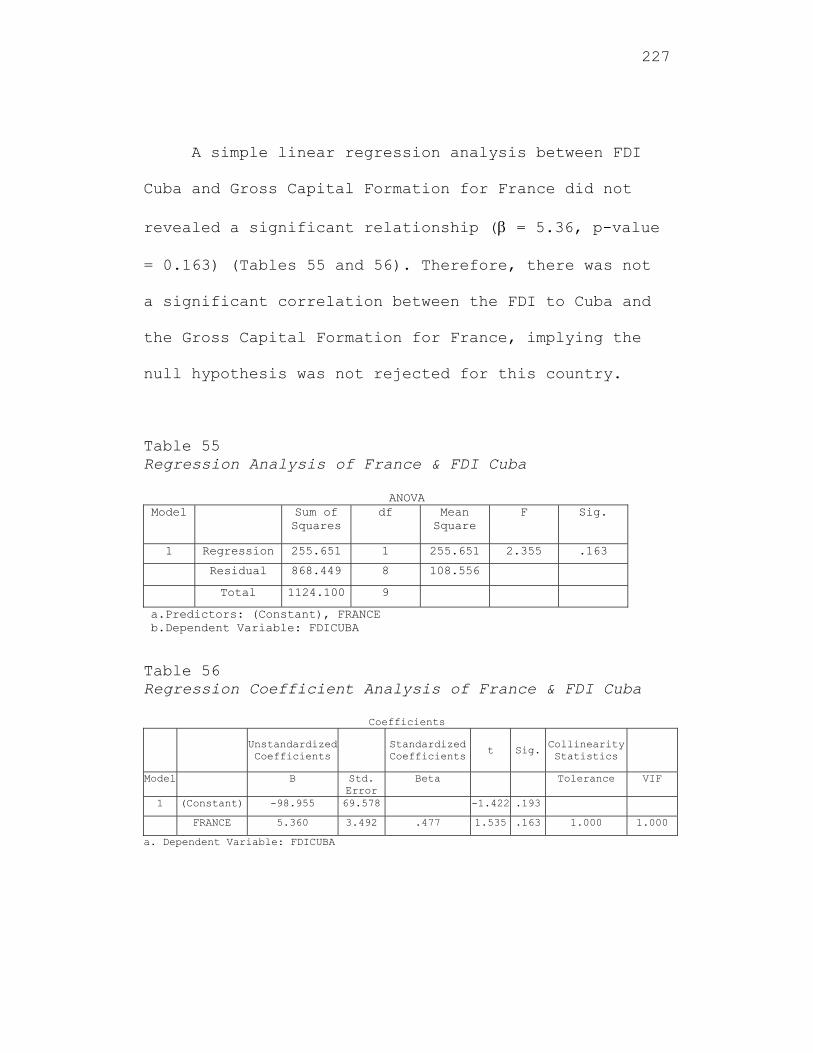
227

A simple linear regression analysis between FDI

Cuba and Gross Capital Formation for France did not

revealed a significant relationship ( = 5.36, p-value

= 0.163) (Tables 55 and 56). Therefore, there was not

a significant correlation between the FDI to Cuba and

the Gross Capital Formation for France, implying the

null hypothesis was not rejected for this country.

Table 55 Regression Analysis of France & FDI Cuba

ANOVA Model Sum of

Squares df Mean

Square F Sig.

1 Regression 255.651 1 255.651 2.355 .163

Residual 868.449 8 108.556

Total 1124.100 9

a.Predictors: (Constant), FRANCE b.Dependent Variable: FDICUBA

Table 56 Regression Coefficient Analysis of France & FDI Cuba

Coefficients

Unstandardized Coefficients

Standardized Coefficients t Sig.

Collinearity Statistics

Model B Std. Error

Beta Tolerance VIF

1 (Constant) -98.955 69.578 -1.422 .193

FRANCE 5.360 3.492 .477 1.535 .163 1.000 1.000

a. Dependent Variable: FDICUBA

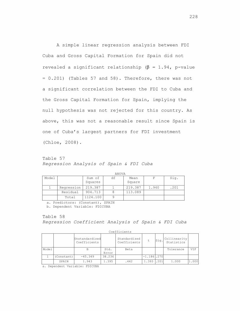
228

A simple linear regression analysis between FDI

Cuba and Gross Capital Formation for Spain did not

revealed a significant relationship ( = 1.94, p-value

= 0.201) (Tables 57 and 58). Therefore, there was not

a significant correlation between the FDI to Cuba and

the Gross Capital Formation for Spain, implying the

null hypothesis was not rejected for this country. As

above, this was not a reasonable result since Spain is

one of Cuba’s largest partners for FDI investment

(Chloe, 2008).

Table 57 Regression Analysis of Spain & FDI Cuba

ANOVA Model Sum of

Squares df Mean

Square F Sig.

1 Regression 219.387 1 219.387 1.940 .201 Residual 904.713 8 113.089

Total 1124.100 9

a. Predictors: (Constant), SPAIN b. Dependent Variable: FDICUBA

Table 58 Regression Coefficient Analysis of Spain & FDI Cuba

Coefficients

Unstandardized Coefficients

Standardized Coefficients

t Sig. Collinearity Statistics

Model B Std. Error

Beta Tolerance VIF

1 (Constant) -45.349 38.236 -1.186 .270

SPAIN 1.943 1.395 .442 1.393 .201 1.000 1.000

a. Dependent Variable: FDICUBA

229

Results for Category II (Developing Countries) Using the Independent Variable, Gross Fixed Capital Formation

The multiple regression analysis, with FDI to

Cuba as the dependent variable and Gross Fixed Capital

Formation for the developing countries, China, India

and the Russian Federation as the independent

variables, did not revealed a significant

relationship. From the ANOVA, the F-value = 3.524 with

a p-value = 0.089 implying that the model was not

significant (Table 59). This was also seen from the

multiple regression analysis where the beta

coefficient was not significant, implying the null

hypothesis was not rejected for these countries (Table

60). This result was surprising as the Russian

Federation and China have been providing significant

FDI to Cuba. From the collinearity diagnostics, the

variance inflation factor (VIF) was 3.011, 2.684 and

1.204 for China, India and the Russian Federation,

respectively, which did not imply a major

multicollinearity problem. (As stated before a VIF

greater than 5 is usually an indication of a

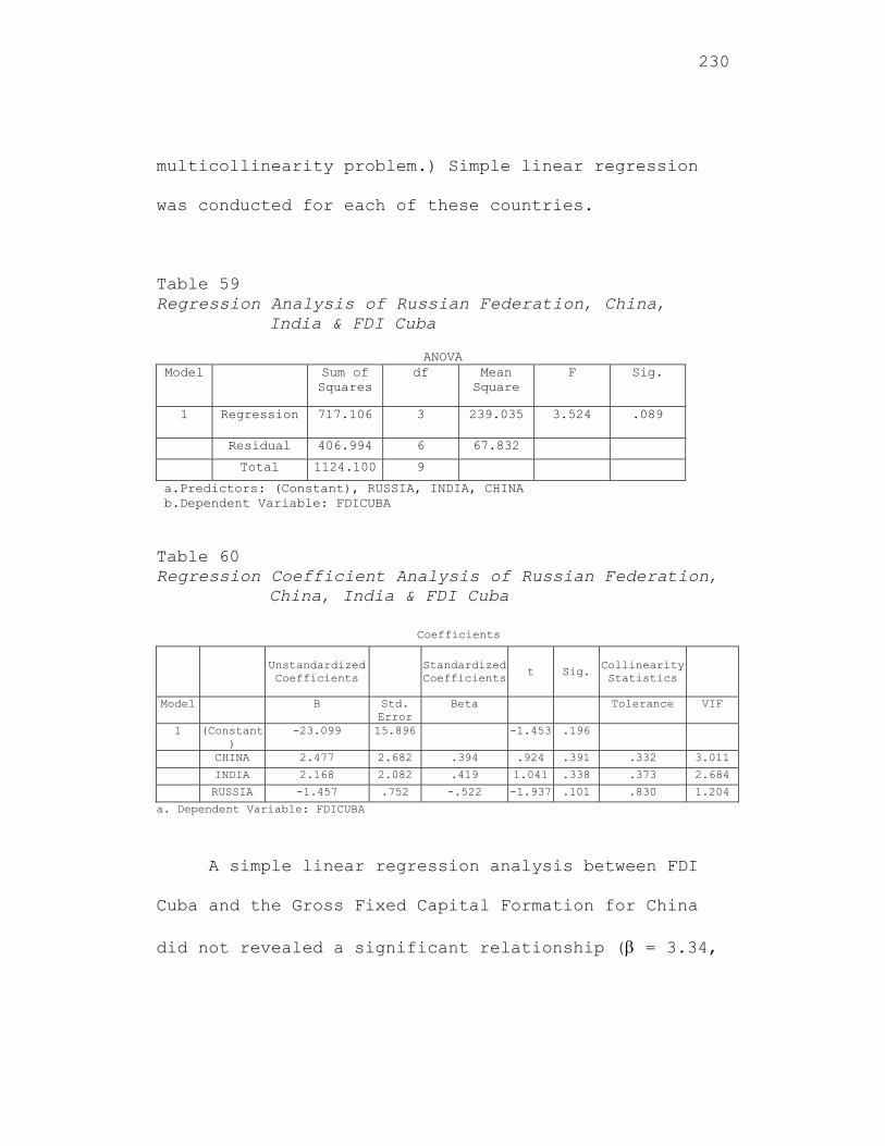
230

multicollinearity problem.) Simple linear regression

was conducted for each of these countries.

Table 59 Regression Analysis of Russian Federation, China,

India & FDI Cuba

ANOVA Model Sum of

Squares df Mean

Square F Sig.

1 Regression 717.106 3 239.035 3.524 .089

Residual 406.994 6 67.832

Total 1124.100 9

a.Predictors: (Constant), RUSSIA, INDIA, CHINA b.Dependent Variable: FDICUBA Table 60 Regression Coefficient Analysis of Russian Federation,

China, India & FDI Cuba

Coefficients

Unstandardized Coefficients

Standardized Coefficients t Sig.

Collinearity Statistics

Model B Std. Error

Beta Tolerance VIF

1 (Constant)

-23.099 15.896 -1.453 .196

CHINA 2.477 2.682 .394 .924 .391 .332 3.011

INDIA 2.168 2.082 .419 1.041 .338 .373 2.684

RUSSIA -1.457 .752 -.522 -1.937 .101 .830 1.204

a. Dependent Variable: FDICUBA

A simple linear regression analysis between FDI

Cuba and the Gross Fixed Capital Formation for China

did not revealed a significant relationship ( = 3.34,

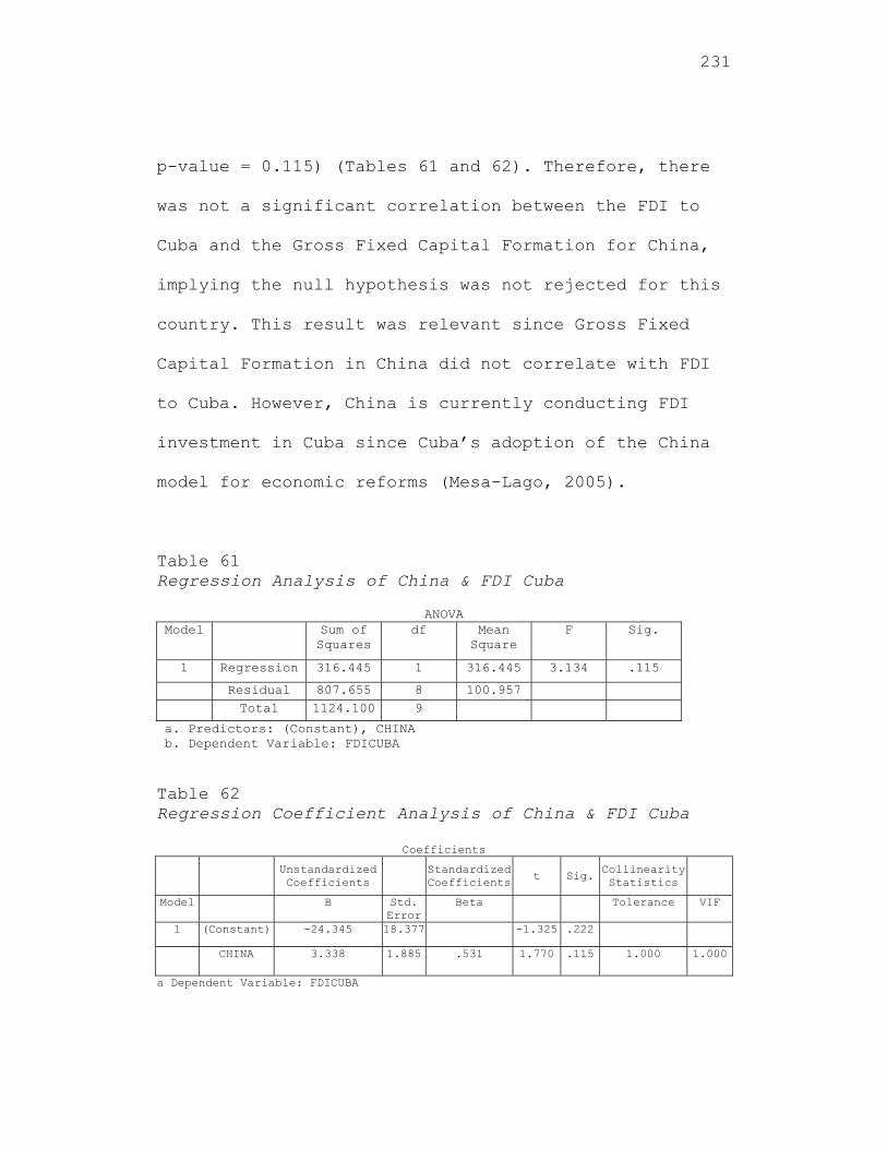
231

p-value = 0.115) (Tables 61 and 62). Therefore, there

was not a significant correlation between the FDI to

Cuba and the Gross Fixed Capital Formation for China,

implying the null hypothesis was not rejected for this

country. This result was relevant since Gross Fixed

Capital Formation in China did not correlate with FDI

to Cuba. However, China is currently conducting FDI

investment in Cuba since Cuba’s adoption of the China

model for economic reforms (Mesa-Lago, 2005).

Table 61 Regression Analysis of China & FDI Cuba

ANOVA Model Sum of

Squares df Mean

Square F Sig.

1 Regression 316.445 1 316.445 3.134 .115

Residual 807.655 8 100.957 Total 1124.100 9

a. Predictors: (Constant), CHINA b. Dependent Variable: FDICUBA Table 62 Regression Coefficient Analysis of China & FDI Cuba

Coefficients Unstandardized

Coefficients Standardized

Coefficientst Sig. Collinearity

Statistics

Model B Std. Error

Beta Tolerance VIF

1 (Constant) -24.345 18.377 -1.325 .222

CHINA 3.338 1.885 .531 1.770 .115 1.000 1.000

a Dependent Variable: FDICUBA

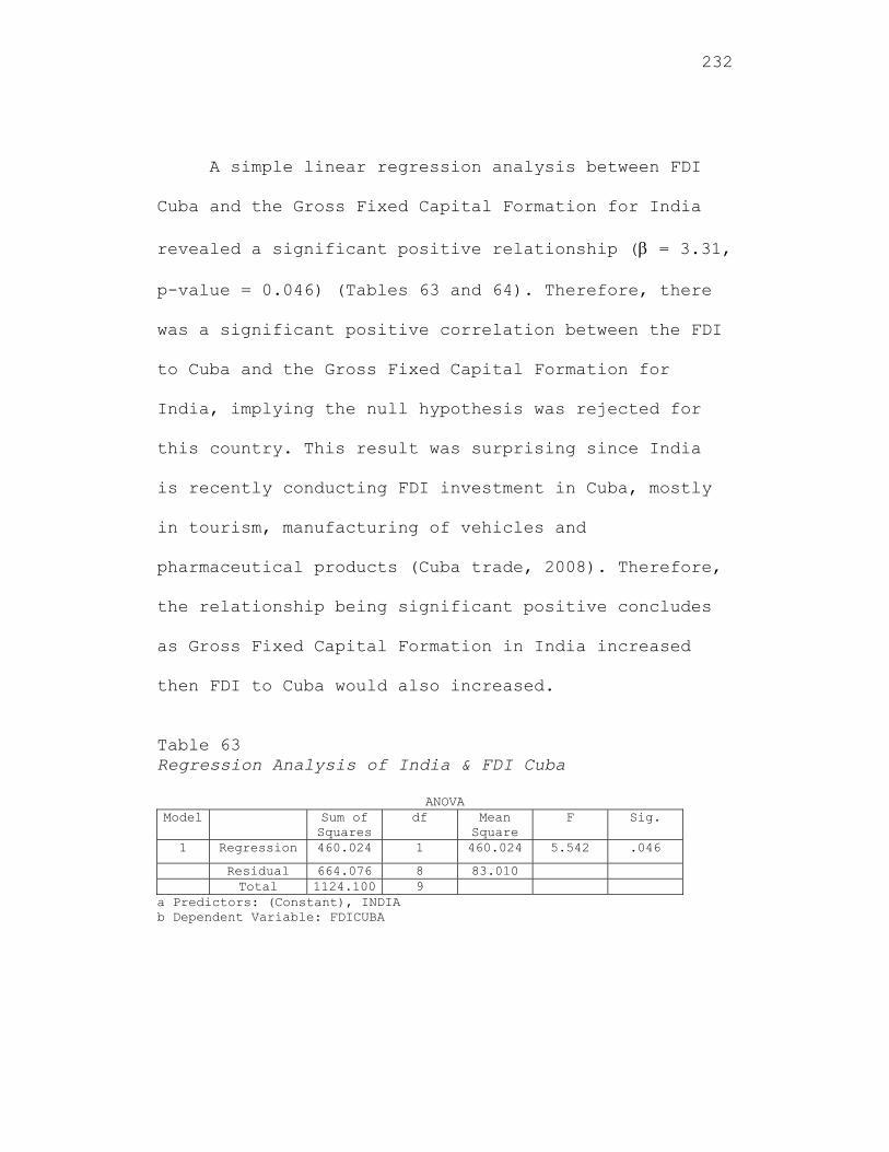
232

A simple linear regression analysis between FDI

Cuba and the Gross Fixed Capital Formation for India

revealed a significant positive relationship ( = 3.31,

p-value = 0.046) (Tables 63 and 64). Therefore, there

was a significant positive correlation between the FDI

to Cuba and the Gross Fixed Capital Formation for

India, implying the null hypothesis was rejected for

this country. This result was surprising since India

is recently conducting FDI investment in Cuba, mostly

in tourism, manufacturing of vehicles and

pharmaceutical products (Cuba trade, 2008). Therefore,

the relationship being significant positive concludes

as Gross Fixed Capital Formation in India increased

then FDI to Cuba would also increased.

Table 63 Regression Analysis of India & FDI Cuba

ANOVA Model Sum of

Squares df Mean

Square F Sig.

1 Regression 460.024 1 460.024 5.542 .046

Residual 664.076 8 83.010 Total 1124.100 9

a Predictors: (Constant), INDIA b Dependent Variable: FDICUBA

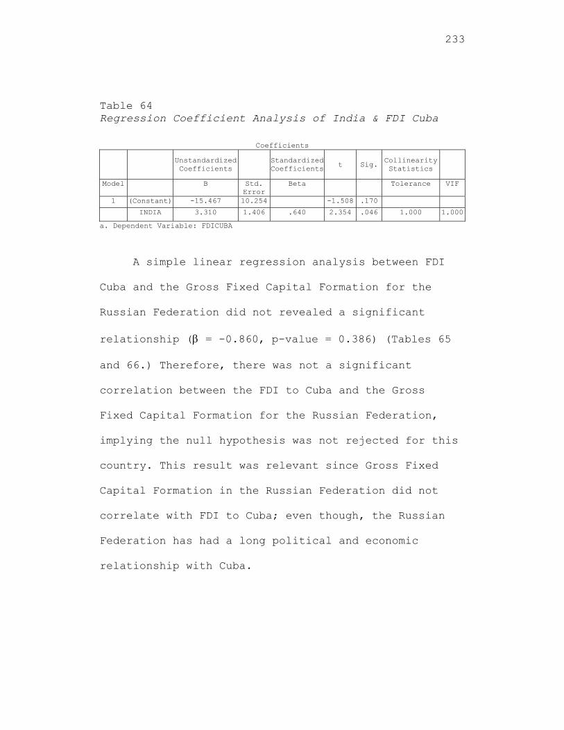
233

Table 64 Regression Coefficient Analysis of India & FDI Cuba

Coefficients

Unstandardized Coefficients

Standardized Coefficients t Sig.

Collinearity Statistics

Model B Std. Error

Beta Tolerance VIF

1 (Constant) -15.467 10.254 -1.508 .170

INDIA 3.310 1.406 .640 2.354 .046 1.000 1.000

a. Dependent Variable: FDICUBA

A simple linear regression analysis between FDI

Cuba and the Gross Fixed Capital Formation for the

Russian Federation did not revealed a significant

relationship ( = -0.860, p-value = 0.386) (Tables 65

and 66.) Therefore, there was not a significant

correlation between the FDI to Cuba and the Gross

Fixed Capital Formation for the Russian Federation,

implying the null hypothesis was not rejected for this

country. This result was relevant since Gross Fixed

Capital Formation in the Russian Federation did not

correlate with FDI to Cuba; even though, the Russian

Federation has had a long political and economic

relationship with Cuba.

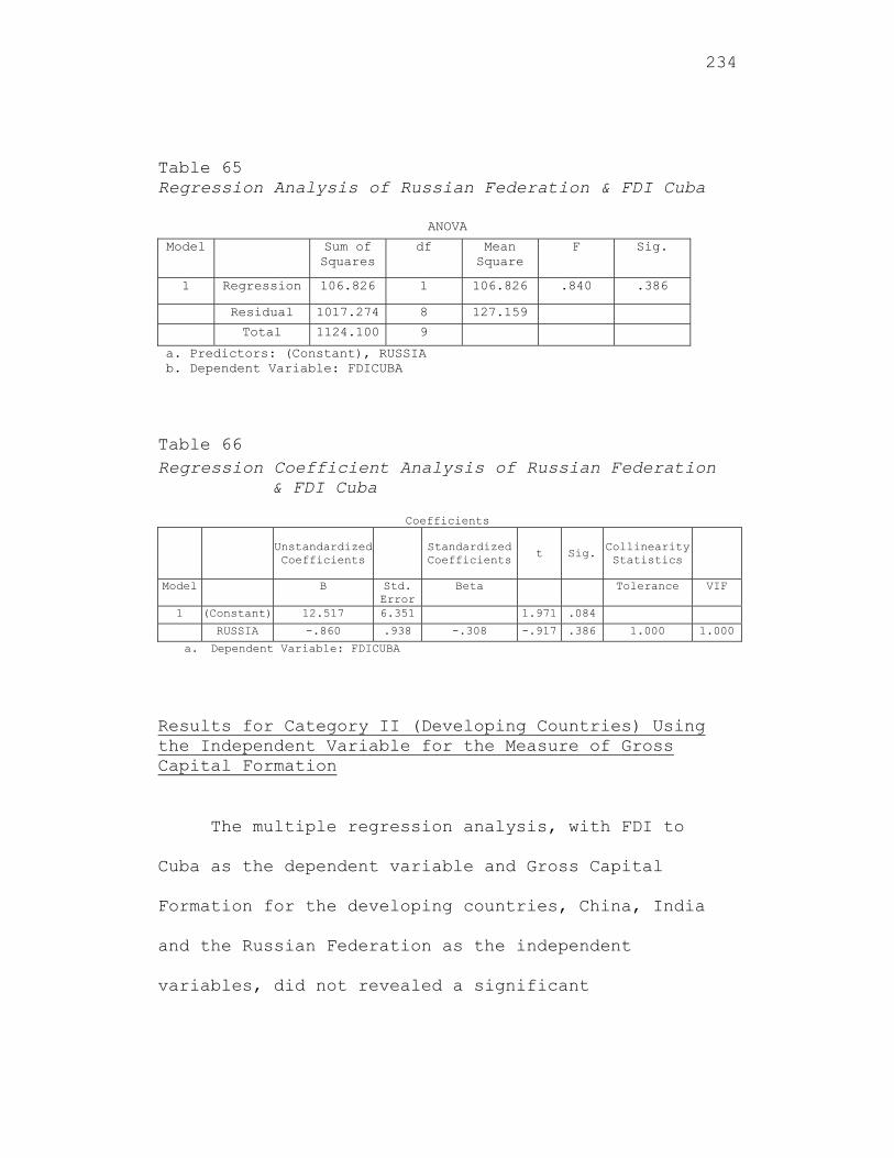
234

Table 65 Regression Analysis of Russian Federation & FDI Cuba

ANOVA

Model Sum of Squares

df Mean Square

F Sig.

1 Regression 106.826 1 106.826 .840 .386

Residual 1017.274 8 127.159

Total 1124.100 9

a. Predictors: (Constant), RUSSIA b. Dependent Variable: FDICUBA

Table 66 Regression Coefficient Analysis of Russian Federation

& FDI Cuba

Coefficients

Unstandardized Coefficients

Standardized Coefficients

t Sig. Collinearity Statistics

Model B Std. Error

Beta Tolerance VIF

1 (Constant) 12.517 6.351 1.971 .084

RUSSIA -.860 .938 -.308 -.917 .386 1.000 1.000

a. Dependent Variable: FDICUBA

Results for Category II (Developing Countries) Using the Independent Variable for the Measure of Gross Capital Formation

The multiple regression analysis, with FDI to

Cuba as the dependent variable and Gross Capital

Formation for the developing countries, China, India

and the Russian Federation as the independent

variables, did not revealed a significant

235

relationship. From the ANOVA, the F-value = 2.673 with

a p-value = 0.141, implying that the model was not

significant (Table 67). This was also seen from the

multiple regression analysis where the beta

coefficient was not significant, implying the null

hypothesis was not rejected for these countries (Table

68). Therefore, there was not a significant

correlation between the FDI to Cuba and the Gross

Capital Formation for these developing countries,

China, India and the Russian Federation. This result

was surprising as the Russian Federation and China had

been providing significant FDI to Cuba. From the

collinearity diagnostics, the variance inflation

factor (VIF) was 5.581, 6.668 and 1.638 for China,

India and the Russian Federation, respectively, which

implied a major multicollinearity problem. (As stated

before a VIF greater than 5 is usually an indication

of a multicollinearity problem.) This implies that two

of the three independent variables are highly

correlated and cannot be utilized for multiple

regression analysis. A correlation analysis further

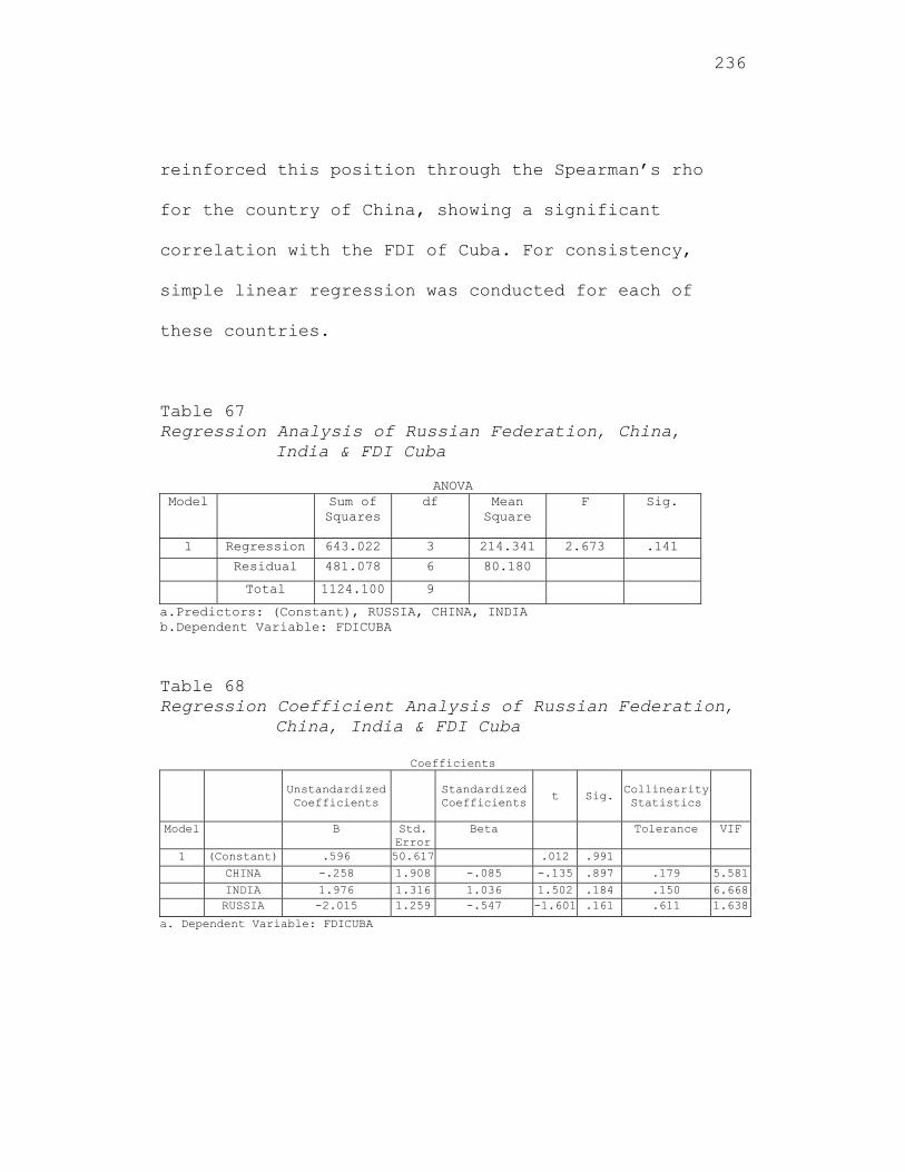
236

reinforced this position through the Spearman’s rho

for the country of China, showing a significant

correlation with the FDI of Cuba. For consistency,

simple linear regression was conducted for each of

these countries.

Table 67 Regression Analysis of Russian Federation, China,

India & FDI Cuba

ANOVA Model Sum of

Squares df Mean

Square F Sig.

1 Regression 643.022 3 214.341 2.673 .141

Residual 481.078 6 80.180

Total 1124.100 9

a.Predictors: (Constant), RUSSIA, CHINA, INDIA b.Dependent Variable: FDICUBA

Table 68 Regression Coefficient Analysis of Russian Federation,

China, India & FDI Cuba

Coefficients

Unstandardized Coefficients

Standardized Coefficients

t Sig. Collinearity Statistics

Model B Std. Error

Beta Tolerance VIF

1 (Constant) .596 50.617 .012 .991

CHINA -.258 1.908 -.085 -.135 .897 .179 5.581

INDIA 1.976 1.316 1.036 1.502 .184 .150 6.668 RUSSIA -2.015 1.259 -.547 -1.601 .161 .611 1.638

a. Dependent Variable: FDICUBA

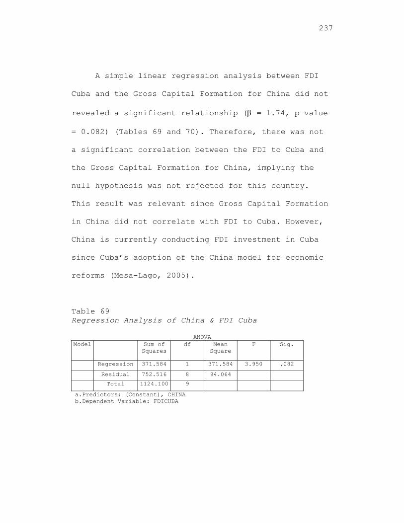
237

A simple linear regression analysis between FDI

Cuba and the Gross Capital Formation for China did not

revealed a significant relationship ( = 1.74, p-value

= 0.082) (Tables 69 and 70). Therefore, there was not

a significant correlation between the FDI to Cuba and

the Gross Capital Formation for China, implying the

null hypothesis was not rejected for this country.

This result was relevant since Gross Capital Formation

in China did not correlate with FDI to Cuba. However,

China is currently conducting FDI investment in Cuba

since Cuba’s adoption of the China model for economic

reforms (Mesa-Lago, 2005).

Table 69 Regression Analysis of China & FDI Cuba

ANOVA Model Sum of

Squares df Mean

Square F Sig.

Regression 371.584 1 371.584 3.950 .082

Residual 752.516 8 94.064

Total 1124.100 9

a.Predictors: (Constant), CHINA b.Dependent Variable: FDICUBA

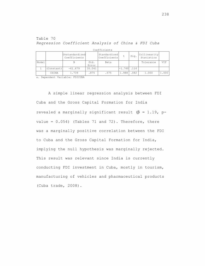
238

Table 70 Regression Coefficient Analysis of China & FDI Cuba

Coefficients

UnstandardizedCoefficients

Standardized Coefficients t Sig.

Collinearity Statistics

Model B Std. Error

Beta Tolerance VIF

1 (Constant) -61.679 35.041 -1.760 .116

CHINA 1.739 .875 .575 1.988 .082 1.000 1.000

a. Dependent Variable: FDICUBA

A simple linear regression analysis between FDI

Cuba and the Gross Capital Formation for India

revealed a marginally significant result ( = 1.19, p-

value = 0.054) (Tables 71 and 72). Therefore, there

was a marginally positive correlation between the FDI

to Cuba and the Gross Capital Formation for India,

implying the null hypothesis was marginally rejected.

This result was relevant since India is currently

conducting FDI investment in Cuba, mostly in tourism,

manufacturing of vehicles and pharmaceutical products

(Cuba trade, 2008).

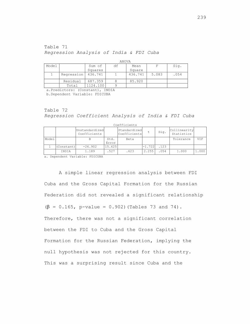
239

Table 71 Regression Analysis of India & FDI Cuba

ANOVA

Model Sum of Squares

df Mean Square

F Sig.

1 Regression 436.741 1 436.741 5.083 .054

Residual 687.359 8 85.920 Total 1124.100 9

a.Predictors: (Constant), INDIA b.Dependent Variable: FDICUBA

Table 72 Regression Coefficient Analysis of India & FDI Cuba

Coefficients Unstandardized

Coefficients Standardized

Coefficientst Sig. Collinearity

Statistics

Model B Std. Error

Beta Tolerance VIF

1 (Constant) -26.902 15.625 -1.722 .123 INDIA 1.189 .527 .623 2.255 .054 1.000 1.000

a. Dependent Variable: FDICUBA

A simple linear regression analysis between FDI

Cuba and the Gross Capital Formation for the Russian

Federation did not revealed a significant relationship

( = 0.165, p-value = 0.902)(Tables 73 and 74).

Therefore, there was not a significant correlation

between the FDI to Cuba and the Gross Capital

Formation for the Russian Federation, implying the

null hypothesis was not rejected for this country.

This was a surprising result since Cuba and the

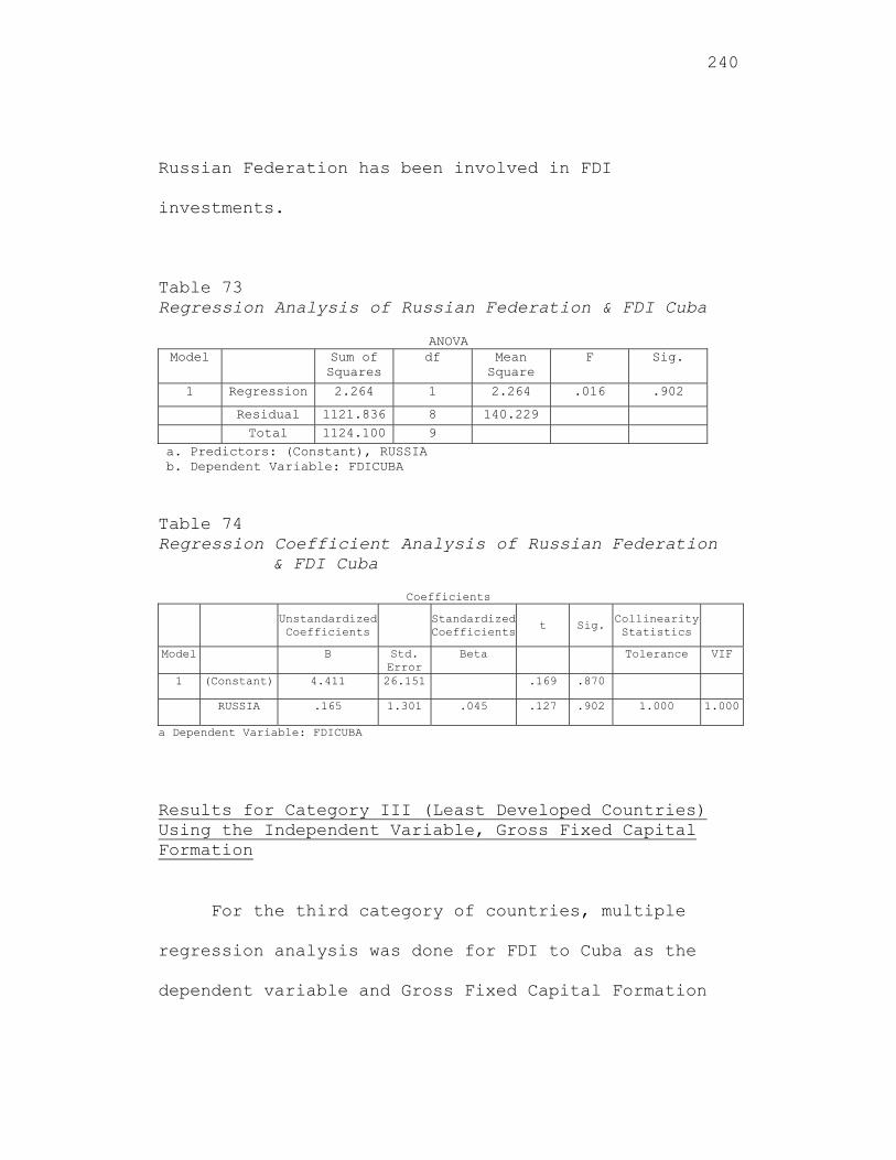
240

Russian Federation has been involved in FDI

investments.

Table 73 Regression Analysis of Russian Federation & FDI Cuba

ANOVA Model Sum of

Squares df Mean

Square F Sig.

1 Regression 2.264 1 2.264 .016 .902

Residual 1121.836 8 140.229 Total 1124.100 9

a. Predictors: (Constant), RUSSIA b. Dependent Variable: FDICUBA

Table 74 Regression Coefficient Analysis of Russian Federation

& FDI Cuba

Coefficients

Unstandardized Coefficients

Standardized Coefficients

t Sig. Collinearity Statistics

Model B Std. Error

Beta Tolerance VIF

1 (Constant) 4.411 26.151 .169 .870

RUSSIA .165 1.301 .045 .127 .902 1.000 1.000

a Dependent Variable: FDICUBA

Results for Category III (Least Developed Countries) Using the Independent Variable, Gross Fixed Capital Formation

For the third category of countries, multiple

regression analysis was done for FDI to Cuba as the

dependent variable and Gross Fixed Capital Formation

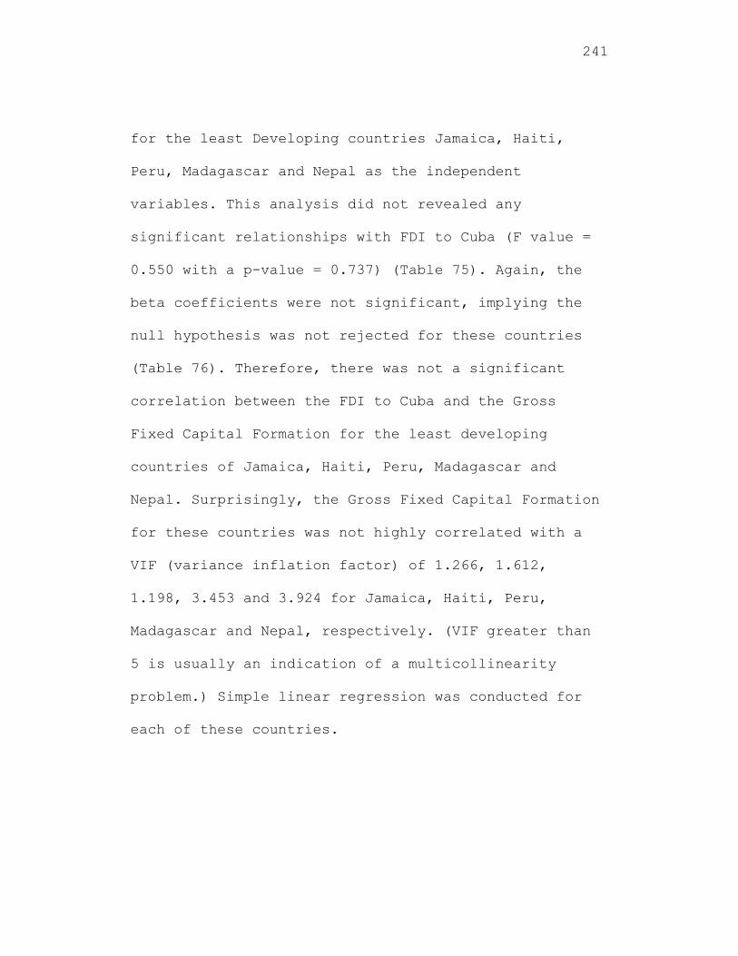
241

for the least Developing countries Jamaica, Haiti,

Peru, Madagascar and Nepal as the independent

variables. This analysis did not revealed any

significant relationships with FDI to Cuba (F value =

0.550 with a p-value = 0.737) (Table 75). Again, the

beta coefficients were not significant, implying the

null hypothesis was not rejected for these countries

(Table 76). Therefore, there was not a significant

correlation between the FDI to Cuba and the Gross

Fixed Capital Formation for the least developing

countries of Jamaica, Haiti, Peru, Madagascar and

Nepal. Surprisingly, the Gross Fixed Capital Formation

for these countries was not highly correlated with a

VIF (variance inflation factor) of 1.266, 1.612,

1.198, 3.453 and 3.924 for Jamaica, Haiti, Peru,

Madagascar and Nepal, respectively. (VIF greater than

5 is usually an indication of a multicollinearity

problem.) Simple linear regression was conducted for

each of these countries.

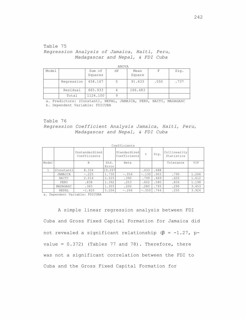
242

Table 75 Regression Analysis of Jamaica, Haiti, Peru,

Madagascar and Nepal, & FDI Cuba

ANOVA Model Sum of

Squares df Mean

Square F Sig.

Regression 458.167 5 91.633 .550 .737

Residual 665.933 4 166.483

Total 1124.100 9

a. Predictors: (Constant), NEPAL, JAMAICA, PERU, HAITI, MADAGASC b. Dependent Variable: FDICUBA Table 76 Regression Coefficient Analysis Jamaica, Haiti, Peru,

Madagascar and Nepal, & FDI Cuba

Coefficients

Unstandardized Coefficients

Standardized Coefficients

t Sig. Collinearity Statistics

Model B Std. Error

Beta Tolerance VIF

1 (Constant) 8.334 19.267 .433 .688 JAMAICA -.225 1.730 -.056 -.130 .903 .790 1.266 HAITI 2.016 2.525 .390 .799 .469 .620 1.612 PERU .838 1.392 .253 .602 .580 .834 1.198 MADAGASC .365 1.305 .200 .280 .793 .290 3.453 NEPAL -1.820 5.206 -.266 -.350 .744 .255 3.924

a. Dependent Variable: FDICUBA

A simple linear regression analysis between FDI

Cuba and Gross Fixed Capital Formation for Jamaica did

not revealed a significant relationship ( = -1.27, p-

value = 0.372) (Tables 77 and 78). Therefore, there

was not a significant correlation between the FDI to

Cuba and the Gross Fixed Capital Formation for

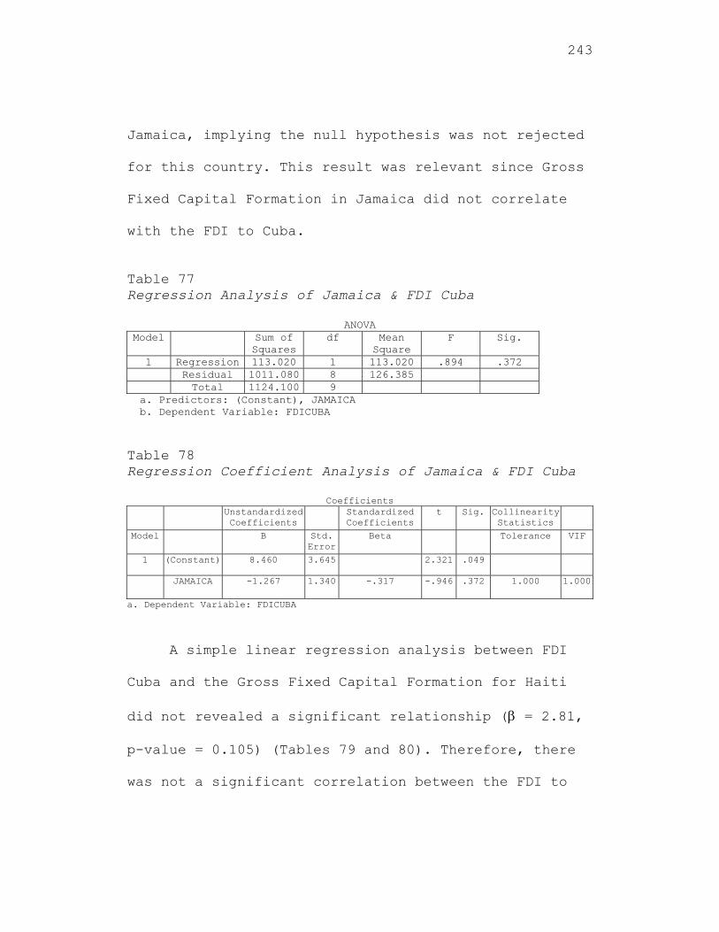
243

Jamaica, implying the null hypothesis was not rejected

for this country. This result was relevant since Gross

Fixed Capital Formation in Jamaica did not correlate

with the FDI to Cuba.

Table 77 Regression Analysis of Jamaica & FDI Cuba

ANOVA Model Sum of

Squares df Mean

Square F Sig.

1 Regression 113.020 1 113.020 .894 .372 Residual 1011.080 8 126.385 Total 1124.100 9

a. Predictors: (Constant), JAMAICA b. Dependent Variable: FDICUBA Table 78 Regression Coefficient Analysis of Jamaica & FDI Cuba

Coefficients Unstandardized

Coefficients Standardized

Coefficients t Sig. Collinearity

Statistics

Model B Std. Error

Beta Tolerance VIF

1 (Constant) 8.460 3.645 2.321 .049

JAMAICA -1.267 1.340 -.317 -.946 .372 1.000 1.000

a. Dependent Variable: FDICUBA

A simple linear regression analysis between FDI

Cuba and the Gross Fixed Capital Formation for Haiti

did not revealed a significant relationship ( = 2.81,

p-value = 0.105) (Tables 79 and 80). Therefore, there

was not a significant correlation between the FDI to

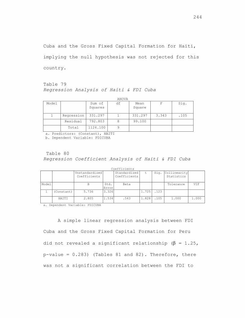
244

Cuba and the Gross Fixed Capital Formation for Haiti,

implying the null hypothesis was not rejected for this

country.

Table 79 Regression Analysis of Haiti & FDI Cuba

ANOVA

Model Sum of Squares

df Mean Square

F Sig.

1 Regression 331.297 1 331.297 3.343 .105

Residual 792.803 8 99.100

Total 1124.100 9

a. Predictors: (Constant), HAITI b. Dependent Variable: FDICUBA

Table 80 Regression Coefficient Analysis of Haiti & FDI Cuba

Coefficients Unstandardized

Coefficients Standardized

Coefficientst Sig. Collinearity

Statistics

Model B Std. Error

Beta Tolerance VIF

1 (Constant) 5.736 3.326 1.725 .123

HAITI 2.805 1.534 .543 1.828 .105 1.000 1.000

a. Dependent Variable: FDICUBA

A simple linear regression analysis between FDI

Cuba and the Gross Fixed Capital Formation for Peru

did not revealed a significant relationship ( = 1.25,

p-value = 0.283) (Tables 81 and 82). Therefore, there

was not a significant correlation between the FDI to

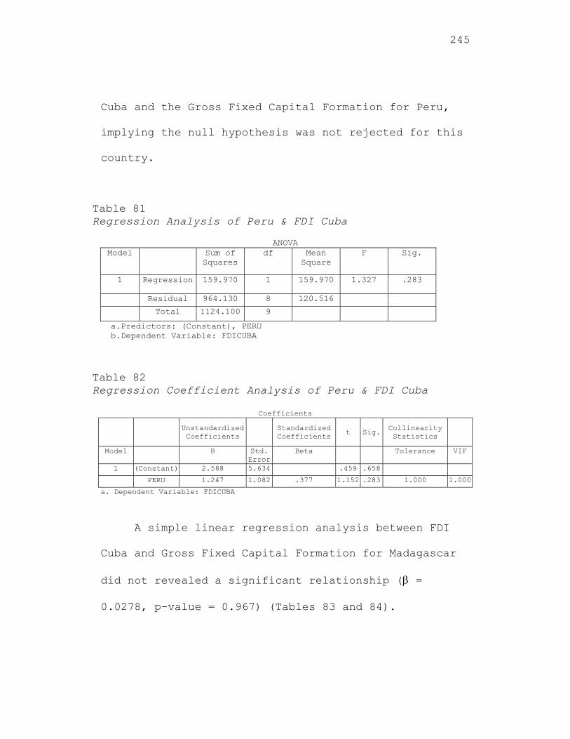
245

Cuba and the Gross Fixed Capital Formation for Peru,

implying the null hypothesis was not rejected for this

country.

Table 81 Regression Analysis of Peru & FDI Cuba

ANOVA Model Sum of

Squares df Mean

Square F Sig.

1 Regression 159.970 1 159.970 1.327 .283

Residual 964.130 8 120.516

Total 1124.100 9

a.Predictors: (Constant), PERU b.Dependent Variable: FDICUBA

Table 82 Regression Coefficient Analysis of Peru & FDI Cuba

Coefficients

Unstandardized Coefficients

Standardized Coefficients

t Sig. Collinearity Statistics

Model B Std. Error

Beta Tolerance VIF

1 (Constant) 2.588 5.634 .459 .658

PERU 1.247 1.082 .377 1.152 .283 1.000 1.000

a. Dependent Variable: FDICUBA

A simple linear regression analysis between FDI

Cuba and Gross Fixed Capital Formation for Madagascar

did not revealed a significant relationship ( =

0.0278, p-value = 0.967) (Tables 83 and 84).

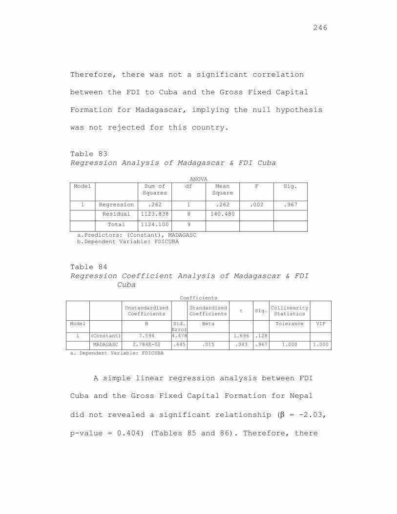
246

Therefore, there was not a significant correlation

between the FDI to Cuba and the Gross Fixed Capital

Formation for Madagascar, implying the null hypothesis

was not rejected for this country.

Table 83 Regression Analysis of Madagascar & FDI Cuba

ANOVA Model Sum of

Squares df Mean

Square F Sig.

1 Regression .262 1 .262 .002 .967

Residual 1123.838 8 140.480

Total 1124.100 9

a.Predictors: (Constant), MADAGASC b.Dependent Variable: FDICUBA

Table 84 Regression Coefficient Analysis of Madagascar & FDI

Cuba

Coefficients

Unstandardized Coefficients

Standardized Coefficients

t Sig. Collinearity Statistics

Model B Std. Error

Beta Tolerance VIF

1 (Constant) 7.594 4.478 1.696 .128

MADAGASC 2.784E-02 .645 .015 .043 .967 1.000 1.000

a. Dependent Variable: FDICUBA

A simple linear regression analysis between FDI

Cuba and the Gross Fixed Capital Formation for Nepal

did not revealed a significant relationship ( = -2.03,

p-value = 0.404) (Tables 85 and 86). Therefore, there

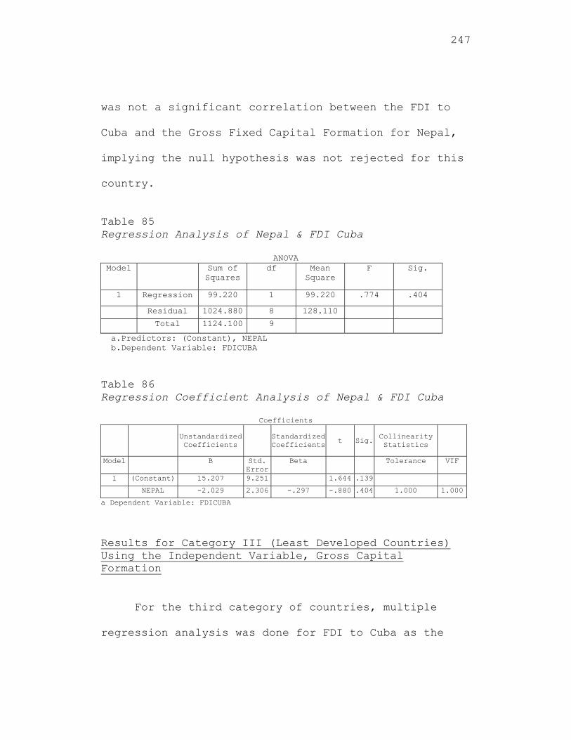
247

was not a significant correlation between the FDI to

Cuba and the Gross Fixed Capital Formation for Nepal,

implying the null hypothesis was not rejected for this

country.

Table 85 Regression Analysis of Nepal & FDI Cuba

ANOVA Model Sum of

Squares df Mean

Square F Sig.

1 Regression 99.220 1 99.220 .774 .404

Residual 1024.880 8 128.110

Total 1124.100 9

a.Predictors: (Constant), NEPAL b.Dependent Variable: FDICUBA

Table 86 Regression Coefficient Analysis of Nepal & FDI Cuba

Coefficients

Unstandardized Coefficients

Standardized Coefficients t Sig.

Collinearity Statistics

Model B Std. Error

Beta Tolerance VIF

1 (Constant) 15.207 9.251 1.644 .139

NEPAL -2.029 2.306 -.297 -.880 .404 1.000 1.000

a Dependent Variable: FDICUBA

Results for Category III (Least Developed Countries) Using the Independent Variable, Gross Capital Formation

For the third category of countries, multiple

regression analysis was done for FDI to Cuba as the

248

dependent variable and Gross Capital Formation for the

least Developing countries, Jamaica, Haiti, Peru,

Madagascar, and Nepal as the independent variables.

This analysis did not revealed any significant

relationships with FDI to Cuba (F value = 0.740 with a

p-value = 0.632) (Table 87). Again, the beta

coefficients were not significant, implying the null

hypothesis was not rejected for these countries (Table

88). Therefore, there was not a significant

correlation between the FDI to Cuba and the Gross

Capital Formation for the least developing countries

of Jamaica, Haiti, Peru, Madagascar, and Nepal. Like

above, the Gross Capital Formation for four out of the

five countries were not highly correlated with VIFs

(variance inflation factor) of 4.259, 1.664, 1.981,

6.521 and 3.737 for Jamaica, Haiti, Peru, Madagascar

and Nepal, respectively. (VIF greater than 5 is

usually an indication of a multicollinearity problem.)

Simple linear regression was conducted for each of

these countries.

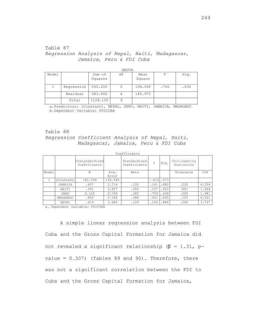
249

Table 87 Regression Analysis of Nepal, Haiti, Madagascar,

Jamaica, Peru & FDI Cuba

ANOVA Model Sum of

Squares df Mean

Square F Sig.

1 Regression 540.200 5 108.040 .740 .632

Residual 583.900 4 145.975

Total 1124.100 9

a.Predictors: (Constant), NEPAL, PERU, HAITI, JAMAICA, MADAGASC b.Dependent Variable: FDICUBA Table 88 Regression Coefficient Analysis of Nepal, Haiti,

Madagascar, Jamaica, Peru & FDI Cuba

Coefficients

Unstandardized Coefficients

Standardized Coefficients

t Sig. Collinearity Statistics

Model B Std. Error

Beta Tolerance VIF

1 (Constant) -83.599 136.545 -.612 .573 JAMAICA .437 2.714 .120 .161 .880 .235 4.259 HAITI .301 2.827 .050 .107 .920 .601 1.664 PERU 2.124 2.799 .385 .759 .490 .505 1.981 MADAGASC .920 2.184 .388 .421 .695 .153 6.521 NEPAL .419 2.686 .109 .156 .884 .268 3.737

a. Dependent Variable: FDICUBA

A simple linear regression analysis between FDI

Cuba and the Gross Capital Formation for Jamaica did

not revealed a significant relationship ( = 1.31, p-

value = 0.307) (Tables 89 and 90). Therefore, there

was not a significant correlation between the FDI to

Cuba and the Gross Capital Formation for Jamaica,

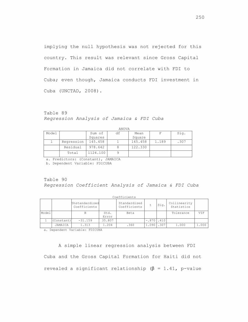
250

implying the null hypothesis was not rejected for this

country. This result was relevant since Gross Capital

Formation in Jamaica did not correlate with FDI to

Cuba; even though, Jamaica conducts FDI investment in

Cuba (UNCTAD, 2008).

Table 89 Regression Analysis of Jamaica & FDI Cuba

ANOVA Model Sum of

Squares df Mean

Square F Sig.

1 Regression 145.458 1 145.458 1.189 .307

Residual 978.642 8 122.330

Total 1124.100 9

a. Predictors: (Constant), JAMAICA b. Dependent Variable: FDICUBA

Table 90 Regression Coefficient Analysis of Jamaica & FDI Cuba

Coefficients

Unstandardized Coefficients

Standardized Coefficients t Sig.

Collinearity Statistics

Model B Std. Error

Beta Tolerance VIF

1 (Constant) -31.159 35.807 -.870 .410 JAMAICA 1.313 1.204 .360 1.090 .307 1.000 1.000

a. Dependent Variable: FDICUBA

A simple linear regression analysis between FDI

Cuba and the Gross Capital Formation for Haiti did not

revealed a significant relationship ( = 1.41, p-value

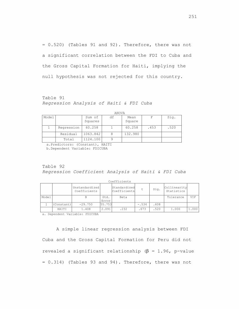
251

= 0.520) (Tables 91 and 92). Therefore, there was not

a significant correlation between the FDI to Cuba and

the Gross Capital Formation for Haiti, implying the

null hypothesis was not rejected for this country.

Table 91 Regression Analysis of Haiti & FDI Cuba

ANOVA Model Sum of

Squares df Mean

Square F Sig.

1 Regression 60.258 1 60.258 .453 .520

Residual 1063.842 8 132.980

Total 1124.100 9

a.Predictors: (Constant), HAITI b.Dependent Variable: FDICUBA Table 92 Regression Coefficient Analysis of Haiti & FDI Cuba

Coefficients

Unstandardized Coefficients

Standardized Coefficients

t Sig. Collinearity Statistics

Model B Std. Error

Beta Tolerance VIF

1 (Constant) -29.750 55.753 -.534 .608

HAITI 1.408 2.091 .232 .673 .520 1.000 1.000

a. Dependent Variable: FDICUBA

A simple linear regression analysis between FDI

Cuba and the Gross Capital Formation for Peru did not

revealed a significant relationship ( = 1.96, p-value

= 0.314) (Tables 93 and 94). Therefore, there was not

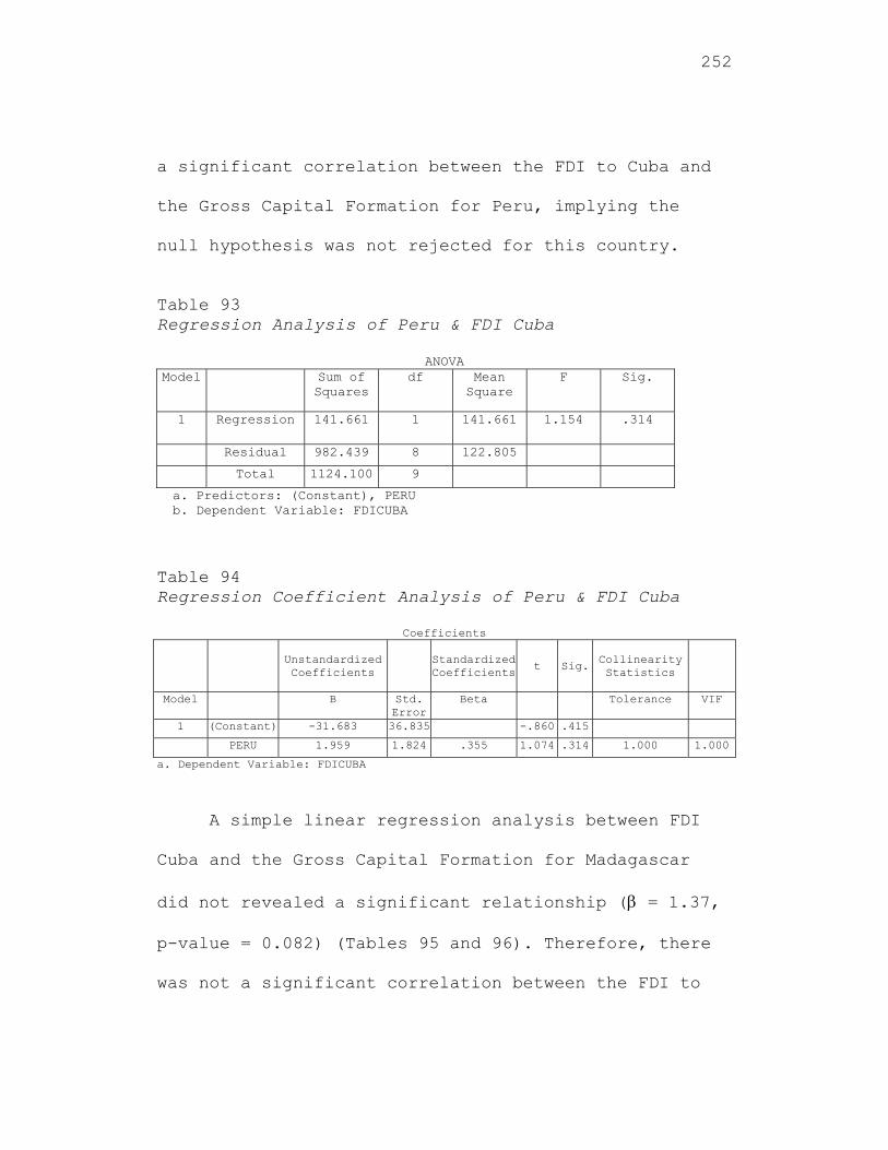
252

a significant correlation between the FDI to Cuba and

the Gross Capital Formation for Peru, implying the

null hypothesis was not rejected for this country.

Table 93 Regression Analysis of Peru & FDI Cuba

ANOVA Model Sum of

Squares df Mean

Square F Sig.

1 Regression 141.661 1 141.661 1.154 .314

Residual 982.439 8 122.805

Total 1124.100 9

a. Predictors: (Constant), PERU b. Dependent Variable: FDICUBA Table 94 Regression Coefficient Analysis of Peru & FDI Cuba

Coefficients

Unstandardized Coefficients

Standardized Coefficients t Sig.

Collinearity Statistics

Model B Std. Error

Beta Tolerance VIF

1 (Constant) -31.683 36.835 -.860 .415

PERU 1.959 1.824 .355 1.074 .314 1.000 1.000

a. Dependent Variable: FDICUBA

A simple linear regression analysis between FDI

Cuba and the Gross Capital Formation for Madagascar

did not revealed a significant relationship ( = 1.37,

p-value = 0.082) (Tables 95 and 96). Therefore, there

was not a significant correlation between the FDI to

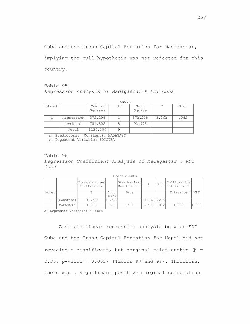
253

Cuba and the Gross Capital Formation for Madagascar,

implying the null hypothesis was not rejected for this

country.

Table 95 Regression Analysis of Madagascar & FDI Cuba

ANOVA Model Sum of

Squares df Mean

Square F Sig.

1 Regression 372.298 1 372.298 3.962 .082

Residual 751.802 8 93.975

Total 1124.100 9

a. Predictors: (Constant), MADAGASC b. Dependent Variable: FDICUBA

Table 96 Regression Coefficient Analysis of Madagascar & FDI Cuba

Coefficients

Unstandardized Coefficients

Standardized Coefficients t Sig.

Collinearity Statistics

Model B Std. Error

Beta Tolerance VIF

1 (Constant) -18.522 13.526 -1.369 .208

MADAGASC 1.366 .686 .575 1.990 .082 1.000 1.000

a. Dependent Variable: FDICUBA

A simple linear regression analysis between FDI

Cuba and the Gross Capital Formation for Nepal did not

revealed a significant, but marginal relationship ( =

2.35, p-value = 0.062) (Tables 97 and 98). Therefore,

there was a significant positive marginal correlation

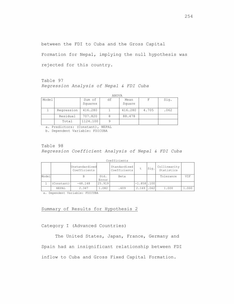
254

between the FDI to Cuba and the Gross Capital

Formation for Nepal, implying the null hypothesis was

rejected for this country.

Table 97 Regression Analysis of Nepal & FDI Cuba

ANOVA Model Sum of

Squares df Mean

Square F Sig.

1 Regression 416.280 1 416.280 4.705 .062

Residual 707.820 8 88.478

Total 1124.100 9

a. Predictors: (Constant), NEPAL b. Dependent Variable: FDICUBA

Table 98 Regression Coefficient Analysis of Nepal & FDI Cuba

Coefficients

Unstandardized Coefficients

Standardized Coefficients t Sig.

Collinearity Statistics

Model B Std. Error

Beta Tolerance VIF

1 (Constant) -48.148 25.919 -1.858 .100

NEPAL 2.347 1.082 .609 2.169 .062 1.000 1.000

a. Dependent Variable: FDICUBA

Summary of Results for Hypothesis 2

Category I (Advanced Countries)

The United States, Japan, France, Germany and

Spain had an insignificant relationship between FDI

inflow to Cuba and Gross Fixed Capital Formation.

255

The United States, Japan, France, Germany and

Spain had an insignificant relationship between FDI

inflow to Cuba and Gross Capital Formation.

Category II (Developing Countries)

Significant positive correlation existed between

FDI inflow to Cuba and Gross Fixed Capital Formation

for India. Insignificant relationships were found for

China and the Russian Federation.

Insignificant relationship existed between FDI

inflow to Cuba and Gross Capital Formation for China

and the Russian Federation. A marginal positive

correlation was found between the FDI inflow to Cuba

and the Gross Capital Formation in India.

Category III (Least Developing Countries)

Insignificant relationship existed between FDI

inflow to Cuba and Gross Fixed Capital Formation for

Jamaica, Haiti, Peru, Madagascar and Nepal.

256

Insignificant relationship existed between FDI

inflow to Cuba and Gross Capital Formation for

Jamaica, Haiti, Peru, Madagascar, while Nepal showed a

positive marginal result.

Results for Hypothesis 3

FDI to Cuba was the dependent variable. For the

advanced countries, the independent variables were the

Level of Technology for the United States, Japan,

Germany, France and Spain (Sawalha, 2007). The

independent variables for the developing countries

were Level of Technology for China, India and the

Russian Federation (Sawalha, 2007). The independent

variables for the Least Developed Countries (LCD’s)

were Level of Technology for Jamaica, Haiti, Peru,

Madagascar and Nepal. The Republic of Cuba’s Level of

Technology was not included in the model as there were

only three data points. The Level of Technology

hypothesis included two variables, High Technology

Exports (percentage of manufactured Exports) and

Industry value added (percentage of GDP).

257

The third hypothesis to be tested is:

Hypothesis H03: The level of contribution of FDI

inflow to Cuba is not significantly related to

the Level of Technology for the three groups of

countries.

Hypothesis HA3: The level of contribution of FDI

inflow to Cuba is significantly related to the

Level of Technology for the three groups of

countries.

The multiple regression models to test Hypothesis 3

are listed below.

Category I (Advanced Countries)

FDICUBA = αO + α1LEVELTECHUS + α2LEVELTECHJapan +

α3LEVELTECHGermany + α4LEVELTECHFrance +

α5LEVELTECHSpain + ε1

Categories II (Developing Countries)

258

FDICUBA = O + 1LEVELTECHChina + 2LEVELTECHIndia +

3LEVELTECHRussian Federation +ε2

Categories III (Least Developed Countries)

FDICUBA = δ + δ1LEVELTECHJamaica + δ2LEVELTECHHaiti +

δ3LEVELTECHPeru + δ4LEVELTECHMadagascar +

δ5LEVELTECHNepal + ε3

The results were present for both independent

variables high technology exports and industry value

added, for each of the three categories of countries.

Results for High Technology Exports as Measured by Percentage of Manufactured Exports

Pearson Correlation Analysis

A Pearson correlation analysis among the

advanced, developing and least developed of the 13 non

oil-producing countries revealed a significant

negative correlation between High Technology Exports

(percentage of Manufactured Exports) for the country

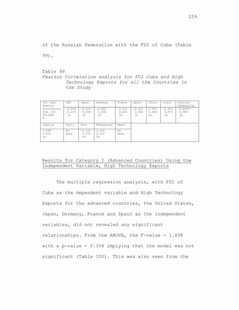
259

of the Russian Federation with the FDI of Cuba (Table

99).

Table 99 Pearson Correlation analysis for FDI Cuba and High

Technology Exports for all the Countries in the Study

FDI Cuba Pearson Correlation Sig. (2-Tailed) N

USA Japan Germany France Spain China India Russian Federation

-0.414 0.235 10

-0.614 0.059 10

-0.402 0.250 10

-0.273 0.445 10

-0.601 0.066 10

0.307 0.389 10

-0.203 0.574 10

-0.820** 0.004 10

Jamaica Haiti Peru Madagascar Nepal

0.292 0.412 10

No Data

-0.316 0.374 10

0.236 0.512 10

No Data

Results for Category I (Advanced Countries) Using the Independent Variable, High Technology Exports

The multiple regression analysis, with FDI of

Cuba as the dependent variable and High Technology

Exports for the advanced countries, the United States,

Japan, Germany, France and Spain as the independent

variables, did not revealed any significant

relationships. From the ANOVA, the F-value = 1.498

with a p-value = 0.358 implying that the model was not

significant (Table 100). This was also seen from the

260

multiple regression analysis where the beta

coefficients were not significant, implying the null

hypothesis was not rejected for these countries

(Table 101). Therefore, there was not a significant

correlation between the FDI of Cuba and High

Technology Exports for these advanced countries, the

United States, Japan, Germany, France and Spain. This

result is surprising as Germany, France and Spain had

been providing significant FDI to Cuba. From the

collinearity diagnostics, the variance inflation

factor (VIF) was 9.365, 12.080, 3.260, 4.088 and

12.033 for the United States, Japan, Germany, France

and Spain, respectively, implying a major

multicollinearity problem. (A VIF greater than 5 is

usually an indication of a multicollinearity problem.)

This implies that three of the five independent

variables are highly correlated and cannot be utilized

for multiple regression analysis. A correlation

analysis further reinforced this position. For

consistency, simple linear regression was conducted

for each of these countries.

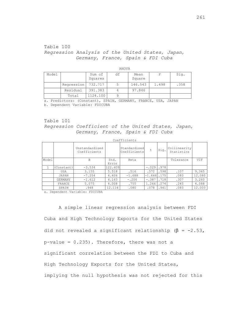
261

Table 100 Regression Analysis of the United States, Japan,

Germany, France, Spain & FDI Cuba

ANOVA

Model Sum of Squares

df Mean Square

F Sig.

Regression 732.717 5 146.543 1.498 .358

Residual 391.383 4 97.846

Total 1124.100 9 a. Predictors: (Constant), SPAIN, GERMANY, FRANCE, USA, JAPAN b. Dependent Variable: FDICUBA

Table 101 Regression Coefficient of the United States, Japan,

Germany, France, Spain & FDI Cuba

Coefficients

Unstandardized Coefficients

Standardized Coefficients t Sig.

Collinearity Statistics

Model B Std. Error

Beta Tolerance VIF

1 (Constant) -3.534 122.409 -.029 .978 USA 3.155 5.518 .516 .572 .598 .107 9.365 JAPAN -7.254 4.406 -1.688 -1.646 .175 .083 12.080 GERMANY -1.612 4.163 -.206 -.387 .718 .307 3.260 FRANCE 5.075 4.008 .755 1.266 .274 .245 4.088 SPAIN .948 12.116 .080 .078 .941 .083 12.003

a. Dependent Variable: FDICUBA

A simple linear regression analysis between FDI

Cuba and High Technology Exports for the United States

did not revealed a significant relationship ( = -2.53,

p-value = 0.235). Therefore, there was not a

significant correlation between the FDI to Cuba and

High Technology Exports for the United States,

implying the null hypothesis was not rejected for this

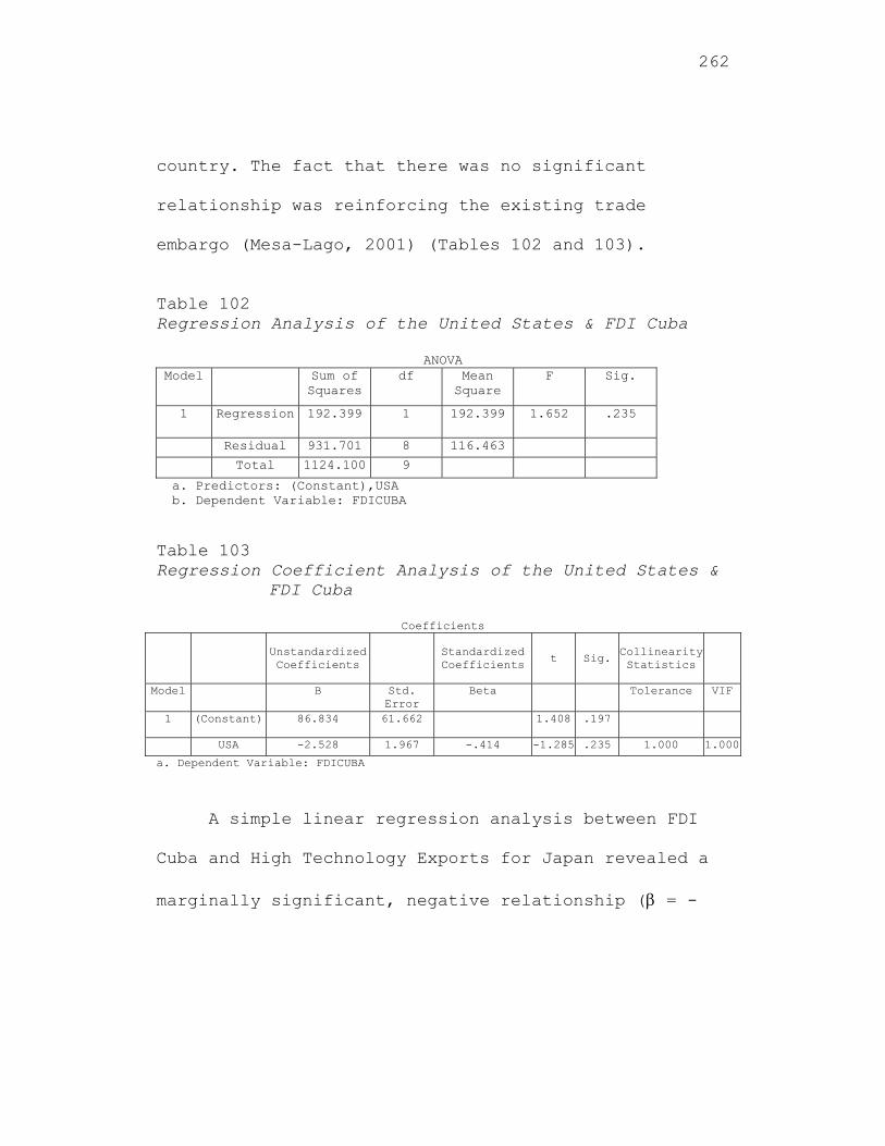
262

country. The fact that there was no significant

relationship was reinforcing the existing trade

embargo (Mesa-Lago, 2001) (Tables 102 and 103).

Table 102 Regression Analysis of the United States & FDI Cuba

ANOVA Model Sum of

Squares df Mean

Square F Sig.

1 Regression 192.399 1 192.399 1.652 .235

Residual 931.701 8 116.463

Total 1124.100 9

a. Predictors: (Constant),USA b. Dependent Variable: FDICUBA Table 103 Regression Coefficient Analysis of the United States &

FDI Cuba

Coefficients

Unstandardized Coefficients

Standardized Coefficients t Sig.

Collinearity Statistics

Model B Std. Error

Beta Tolerance VIF

1 (Constant) 86.834 61.662 1.408 .197

USA -2.528 1.967 -.414 -1.285 .235 1.000 1.000

a. Dependent Variable: FDICUBA

A simple linear regression analysis between FDI

Cuba and High Technology Exports for Japan revealed a

marginally significant, negative relationship ( = -

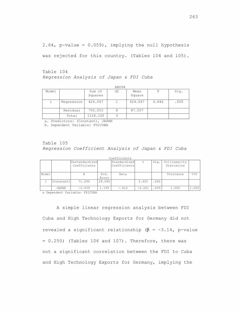
263

2.64, p-value = 0.059), implying the null hypothesis

was rejected for this country. (Tables 104 and 105).

Table 104 Regression Analysis of Japan & FDI Cuba

ANOVA Model Sum of

Squares df Mean

Square F Sig.

1 Regression 424.047 1 424.047 4.846 .059

Residual 700.053 8 87.507

Total 1124.100 9

a. Predictors: (Constant), JAPAN b. Dependent Variable: FDICUBA

Table 105 Regression Coefficient Analysis of Japan & FDI Cuba

Coefficients Unstandardized

Coefficients Standardized

Coefficientst Sig. Collinearity

Statistics

Model B Std. Error

Beta Tolerance VIF

1 (Constant) 71.294 29.040 2.455 .040

JAPAN -2.639 1.199 -.614 -2.201 .059 1.000 1.000

a Dependent Variable: FDICUBA

A simple linear regression analysis between FDI

Cuba and High Technology Exports for Germany did not

revealed a significant relationship ( = -3.14, p-value

= 0.250) (Tables 106 and 107). Therefore, there was

not a significant correlation between the FDI to Cuba

and High Technology Exports for Germany, implying the

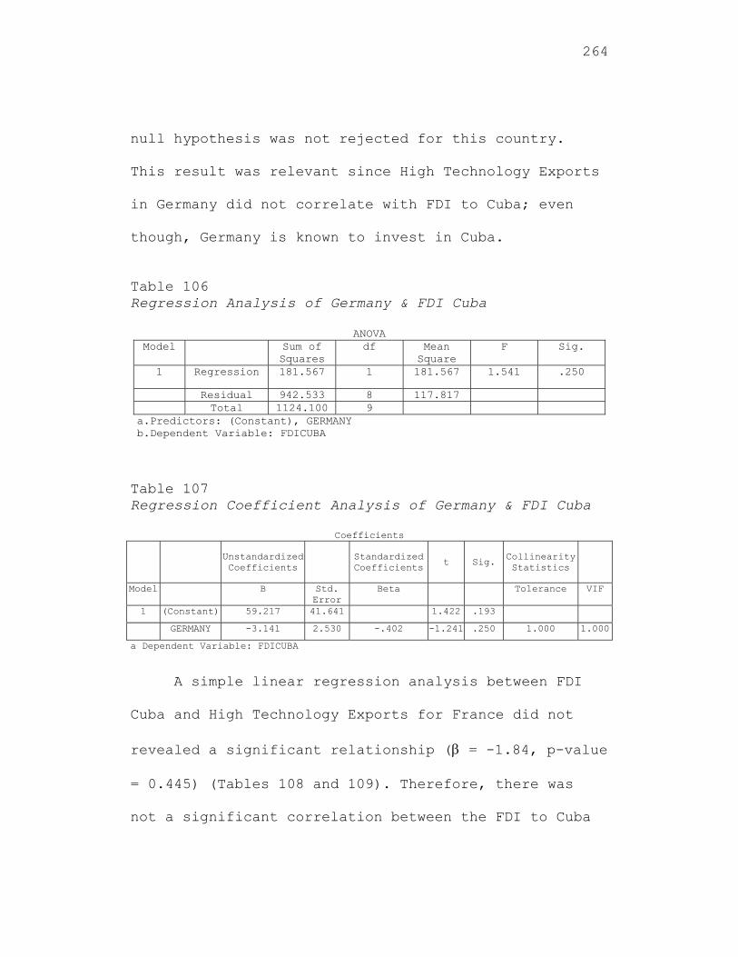
264

null hypothesis was not rejected for this country.

This result was relevant since High Technology Exports

in Germany did not correlate with FDI to Cuba; even

though, Germany is known to invest in Cuba.

Table 106 Regression Analysis of Germany & FDI Cuba

ANOVA Model Sum of

Squares df Mean

Square F Sig.

1 Regression 181.567 1 181.567 1.541 .250

Residual 942.533 8 117.817 Total 1124.100 9

a.Predictors: (Constant), GERMANY b.Dependent Variable: FDICUBA Table 107 Regression Coefficient Analysis of Germany & FDI Cuba

Coefficients

Unstandardized Coefficients

Standardized Coefficients

t Sig. Collinearity Statistics

Model B Std. Error

Beta Tolerance VIF

1 (Constant) 59.217 41.641 1.422 .193

GERMANY -3.141 2.530 -.402 -1.241 .250 1.000 1.000

a Dependent Variable: FDICUBA

A simple linear regression analysis between FDI

Cuba and High Technology Exports for France did not

revealed a significant relationship ( = -1.84, p-value

= 0.445) (Tables 108 and 109). Therefore, there was

not a significant correlation between the FDI to Cuba

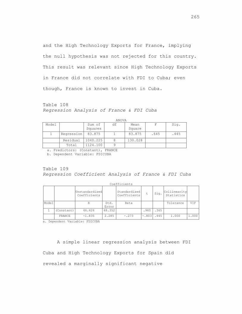
265

and the High Technology Exports for France, implying

the null hypothesis was not rejected for this country.

This result was relevant since High Technology Exports

in France did not correlate with FDI to Cuba; even

though, France is known to invest in Cuba.

Table 108 Regression Analysis of France & FDI Cuba

ANOVA Model Sum of

Squares df Mean

Square F Sig.

1 Regression 83.875 1 83.875 .645 .445

Residual 1040.225 8 130.028 Total 1124.100 9

a. Predictors: (Constant), FRANCE b. Dependent Variable: FDICUBA Table 109 Regression Coefficient Analysis of France & FDI Cuba

Coefficients

Unstandardized Coefficients

Standardized Coefficients

t Sig. Collinearity Statistics

Model B Std. Error

Beta Tolerance VIF

1 (Constant) 46.426 48.352 .960 .365

FRANCE -1.835 2.285 -.273 -.803 .445 1.000 1.000

a. Dependent Variable: FDICUBA

A simple linear regression analysis between FDI

Cuba and High Technology Exports for Spain did

revealed a marginally significant negative

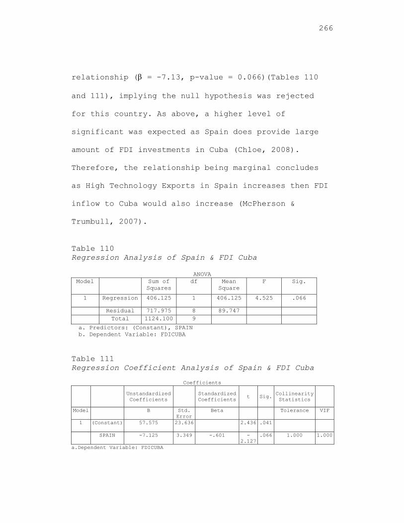
266

relationship ( = -7.13, p-value = 0.066)(Tables 110

and 111), implying the null hypothesis was rejected

for this country. As above, a higher level of

significant was expected as Spain does provide large

amount of FDI investments in Cuba (Chloe, 2008).

Therefore, the relationship being marginal concludes

as High Technology Exports in Spain increases then FDI

inflow to Cuba would also increase (McPherson &

Trumbull, 2007).

Table 110 Regression Analysis of Spain & FDI Cuba

ANOVA Model Sum of

Squares df Mean

Square F Sig.

1 Regression 406.125 1 406.125 4.525 .066

Residual 717.975 8 89.747 Total 1124.100 9

a. Predictors: (Constant), SPAIN b. Dependent Variable: FDICUBA Table 111 Regression Coefficient Analysis of Spain & FDI Cuba

Coefficients

Unstandardized Coefficients

Standardized Coefficients

t Sig. Collinearity Statistics

Model B Std. Error

Beta Tolerance VIF

1 (Constant) 57.575 23.636 2.436 .041

SPAIN -7.125 3.349 -.601 -2.127

.066 1.000 1.000

a.Dependent Variable: FDICUBA

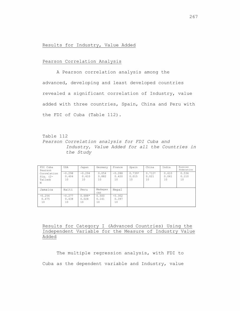
267

Results for Industry, Value Added

Pearson Correlation Analysis

A Pearson correlation analysis among the

advanced, developing and least developed countries

revealed a significant correlation of Industry, value

added with three countries, Spain, China and Peru with

the FDI of Cuba (Table 112).

Table 112 Pearson Correlation analysis for FDI Cuba and

Industry, Value Added for all the Countries in the Study

FDI Cuba Pearson Correlation Sig. (2-Tailed) N

USA Japan Germany France Spain China India Russian Federation

-0.298 0.404 10

-0.294 0.410 10

0.054 0.882 10

-0.288 0.420 10

0.739* 0.015 10

0.712* 0.021 10

0.610 0.061 10

0.536 0.110 10

Jamaica Haiti Peru Madagascar

Nepal

-0.256 0.475 10

-0.277 0.438 10

0.688* 0.028 10

0.500 0.141 10

-0.302 0.397 10

Results for Category I (Advanced Countries) Using the Independent Variable for the Measure of Industry Value Added

The multiple regression analysis, with FDI to

Cuba as the dependent variable and Industry, value

268

added for the advanced countries, the United States,

Japan, Germany, France and Spain as the independent

variables, did not revealed any significant

relationships. From the ANOVA, the F-value = 2.411

with a p-value = 0.207 implying that the model was not

significant (Table 113). This was also seen from the

multiple regression analysis where the beta

coefficients were not significant except for Spain

(Table 114). Therefore, there was not a significant

correlation between the FDI to Cuba and the Industry,

value for the United States, Japan, Germany, France

and Spain, implying the null hypothesis was not

rejected for these countries. This result is

surprising as Germany, France and Spain had been

providing significant FDI to Cuba. From the

collinearity diagnostics, the variance inflation

factor (VIF) was 1501.068, 1530.216, 6.188, 5.078 and

1.908 for the United States, Japan, Germany, France

and Spain, respectively, implying a major

multicollinearity problem. (A VIF greater than 5 is

usually an indication of a multicollinearity problem.)

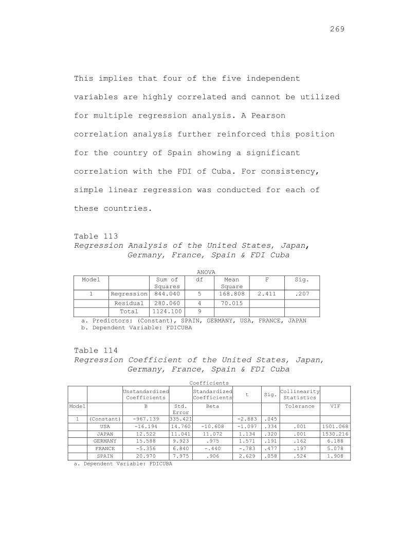
269

This implies that four of the five independent

variables are highly correlated and cannot be utilized

for multiple regression analysis. A Pearson

correlation analysis further reinforced this position

for the country of Spain showing a significant

correlation with the FDI of Cuba. For consistency,

simple linear regression was conducted for each of

these countries.

Table 113 Regression Analysis of the United States, Japan,

Germany, France, Spain & FDI Cuba

ANOVA Model Sum of

Squares df Mean

Square F Sig.

1 Regression 844.040 5 168.808 2.411 .207

Residual 280.060 4 70.015 Total 1124.100 9

a. Predictors: (Constant), SPAIN, GERMANY, USA, FRANCE, JAPAN b. Dependent Variable: FDICUBA Table 114 Regression Coefficient of the United States, Japan,

Germany, France, Spain & FDI Cuba

Coefficients Unstandardized

Coefficients Standardized

Coefficientst Sig. Collinearity

Statistics

Model B Std. Error

Beta Tolerance VIF

1 (Constant) -967.139 335.421 -2.883 .045 USA -16.194 14.760 -10.608 -1.097 .334 .001 1501.068 JAPAN 12.522 11.041 11.072 1.134 .320 .001 1530.216 GERMANY 15.588 9.923 .975 1.571 .191 .162 6.188 FRANCE -5.356 6.840 -.440 -.783 .477 .197 5.078 SPAIN 20.970 7.975 .906 2.629 .058 .524 1.908

a. Dependent Variable: FDICUBA

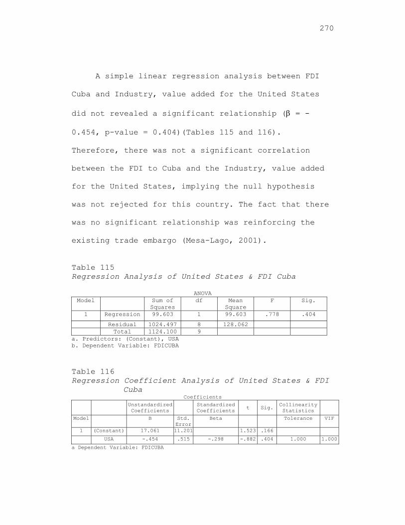
270

A simple linear regression analysis between FDI

Cuba and Industry, value added for the United States

did not revealed a significant relationship ( = -

0.454, p-value = 0.404)(Tables 115 and 116).

Therefore, there was not a significant correlation

between the FDI to Cuba and the Industry, value added

for the United States, implying the null hypothesis

was not rejected for this country. The fact that there

was no significant relationship was reinforcing the

existing trade embargo (Mesa-Lago, 2001).

Table 115 Regression Analysis of United States & FDI Cuba

ANOVA Model Sum of

Squares df Mean

Square F Sig.

1 Regression 99.603 1 99.603 .778 .404

Residual 1024.497 8 128.062 Total 1124.100 9

a. Predictors: (Constant), USA b. Dependent Variable: FDICUBA

Table 116 Regression Coefficient Analysis of United States & FDI

Cuba Coefficients

Unstandardized Coefficients

Standardized Coefficients t Sig.

Collinearity Statistics

Model B Std. Error

Beta Tolerance VIF

1 (Constant) 17.061 11.201 1.523 .166

USA -.454 .515 -.298 -.882 .404 1.000 1.000

a Dependent Variable: FDICUBA

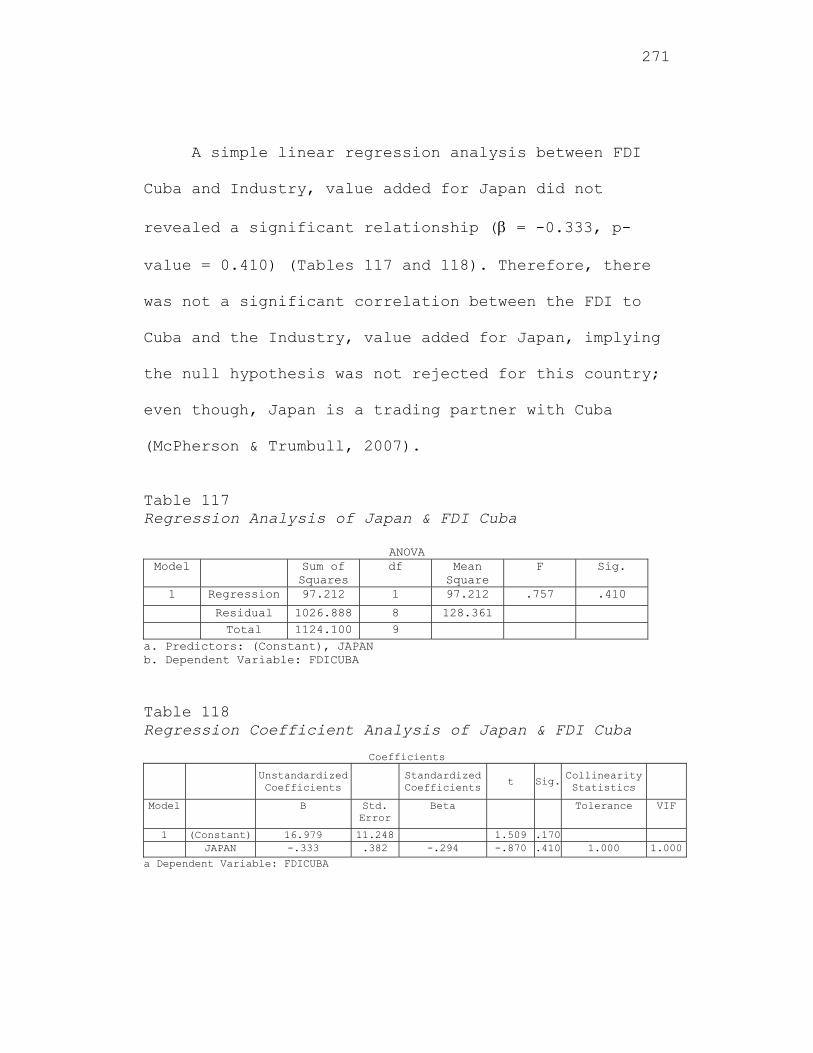
271

A simple linear regression analysis between FDI

Cuba and Industry, value added for Japan did not

revealed a significant relationship ( = -0.333, p-

value = 0.410) (Tables 117 and 118). Therefore, there

was not a significant correlation between the FDI to

Cuba and the Industry, value added for Japan, implying

the null hypothesis was not rejected for this country;

even though, Japan is a trading partner with Cuba

(McPherson & Trumbull, 2007).

Table 117 Regression Analysis of Japan & FDI Cuba

ANOVA Model Sum of

Squares df Mean

Square F Sig.

1 Regression 97.212 1 97.212 .757 .410

Residual 1026.888 8 128.361 Total 1124.100 9

a. Predictors: (Constant), JAPAN b. Dependent Variable: FDICUBA

Table 118 Regression Coefficient Analysis of Japan & FDI Cuba

Coefficients

Unstandardized Coefficients

Standardized Coefficients

t Sig.Collinearity Statistics

Model B Std. Error

Beta Tolerance VIF

1 (Constant) 16.979 11.248 1.509 .170 JAPAN -.333 .382 -.294 -.870 .410 1.000 1.000

a Dependent Variable: FDICUBA

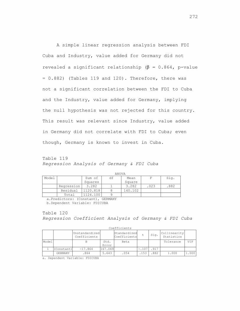
272

A simple linear regression analysis between FDI

Cuba and Industry, value added for Germany did not

revealed a significant relationship ( = 0.864, p-value

= 0.882) (Tables 119 and 120). Therefore, there was

not a significant correlation between the FDI to Cuba

and the Industry, value added for Germany, implying

the null hypothesis was not rejected for this country.

This result was relevant since Industry, value added

in Germany did not correlate with FDI to Cuba; even

though, Germany is known to invest in Cuba.

Table 119 Regression Analysis of Germany & FDI Cuba

ANOVA Model Sum of

Squares df Mean

Square F Sig.

Regression 3.282 1 3.282 .023 .882 Residual 1120.818 8 140.102 Total 1124.100 9

a.Predictors: (Constant), GERMANY b.Dependent Variable: FDICUBA

Table 120 Regression Coefficient Analysis of Germany & FDI Cuba

Coefficients Unstandardized

Coefficients Standardized

Coefficientst Sig. Collinearity

Statistics

Model B Std. Error

Beta Tolerance VIF

1 (Constant) -17.864 167.069 -.107 .917 GERMANY .864 5.643 .054 .153 .882 1.000 1.000

a. Dependent Variable: FDICUBA

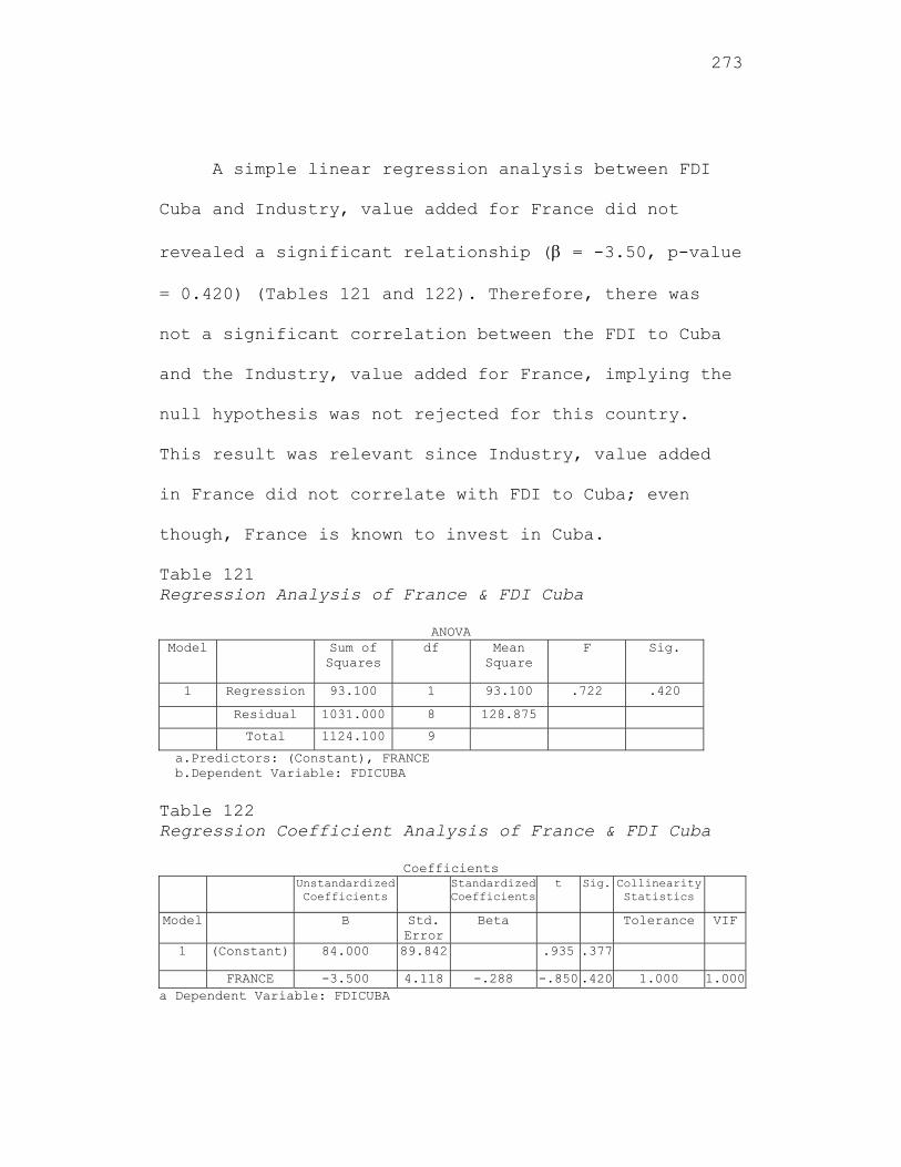
273

A simple linear regression analysis between FDI

Cuba and Industry, value added for France did not

revealed a significant relationship ( = -3.50, p-value

= 0.420) (Tables 121 and 122). Therefore, there was

not a significant correlation between the FDI to Cuba

and the Industry, value added for France, implying the

null hypothesis was not rejected for this country.

This result was relevant since Industry, value added

in France did not correlate with FDI to Cuba; even

though, France is known to invest in Cuba.

Table 121 Regression Analysis of France & FDI Cuba

ANOVA Model Sum of

Squares df Mean

Square F Sig.

1 Regression 93.100 1 93.100 .722 .420

Residual 1031.000 8 128.875

Total 1124.100 9

a.Predictors: (Constant), FRANCE b.Dependent Variable: FDICUBA

Table 122 Regression Coefficient Analysis of France & FDI Cuba

Coefficients Unstandardized

Coefficients Standardized

Coefficientst Sig. Collinearity

Statistics

Model B Std. Error

Beta Tolerance VIF

1 (Constant) 84.000 89.842 .935 .377

FRANCE -3.500 4.118 -.288 -.850 .420 1.000 1.000a Dependent Variable: FDICUBA

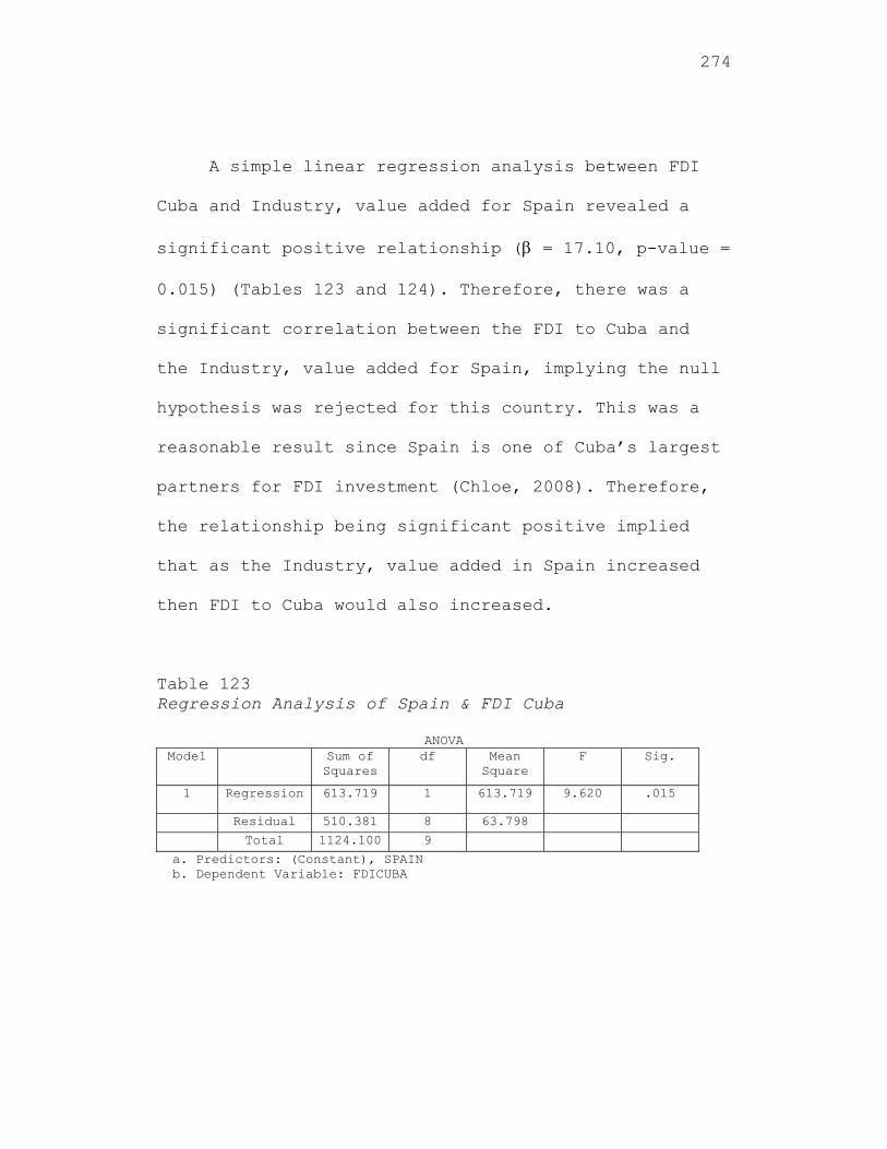
274

A simple linear regression analysis between FDI

Cuba and Industry, value added for Spain revealed a

significant positive relationship ( = 17.10, p-value =

0.015) (Tables 123 and 124). Therefore, there was a

significant correlation between the FDI to Cuba and

the Industry, value added for Spain, implying the null

hypothesis was rejected for this country. This was a

reasonable result since Spain is one of Cuba’s largest

partners for FDI investment (Chloe, 2008). Therefore,

the relationship being significant positive implied

that as the Industry, value added in Spain increased

then FDI to Cuba would also increased.

Table 123 Regression Analysis of Spain & FDI Cuba

ANOVA Model Sum of

Squares df Mean

Square F Sig.

1 Regression 613.719 1 613.719 9.620 .015

Residual 510.381 8 63.798

Total 1124.100 9

a. Predictors: (Constant), SPAIN b. Dependent Variable: FDICUBA

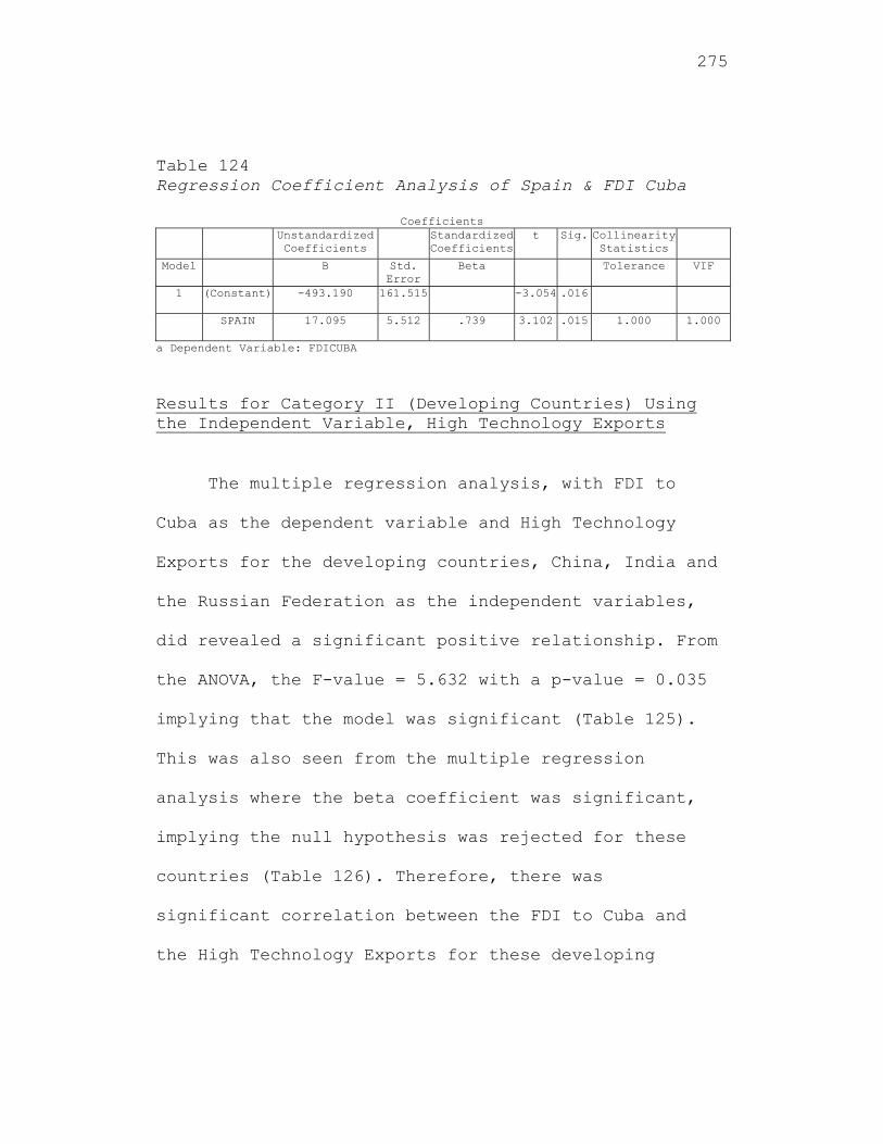
275

Table 124 Regression Coefficient Analysis of Spain & FDI Cuba

Coefficients Unstandardized

Coefficients Standardized

Coefficientst Sig. Collinearity

Statistics

Model B Std. Error

Beta Tolerance VIF

1 (Constant) -493.190 161.515 -3.054 .016

SPAIN 17.095 5.512 .739 3.102 .015 1.000 1.000

a Dependent Variable: FDICUBA

Results for Category II (Developing Countries) Using the Independent Variable, High Technology Exports

The multiple regression analysis, with FDI to

Cuba as the dependent variable and High Technology

Exports for the developing countries, China, India and

the Russian Federation as the independent variables,

did revealed a significant positive relationship. From

the ANOVA, the F-value = 5.632 with a p-value = 0.035

implying that the model was significant (Table 125).

This was also seen from the multiple regression

analysis where the beta coefficient was significant,

implying the null hypothesis was rejected for these

countries (Table 126). Therefore, there was

significant correlation between the FDI to Cuba and

the High Technology Exports for these developing

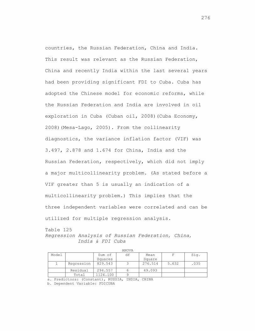
276

countries, the Russian Federation, China and India.

This result was relevant as the Russian Federation,

China and recently India within the last several years

had been providing significant FDI to Cuba. Cuba has

adopted the Chinese model for economic reforms, while

the Russian Federation and India are involved in oil

exploration in Cuba (Cuban oil, 2008)(Cuba Economy,

2008)(Mesa-Lago, 2005). From the collinearity

diagnostics, the variance inflation factor (VIF) was

3.497, 2.878 and 1.674 for China, India and the

Russian Federation, respectively, which did not imply

a major multicollinearity problem. (As stated before a

VIF greater than 5 is usually an indication of a

multicollinearity problem.) This implies that the

three independent variables were correlated and can be

utilized for multiple regression analysis.

Table 125 Regression Analysis of Russian Federation, China,

India & FDI Cuba

ANOVA Model Sum of

Squares df Mean

Square F Sig.

1 Regression 829.543 3 276.514 5.632 .035

Residual 294.557 6 49.093 Total 1124.100 9

a. Predictors: (Constant), RUSSIA, INDIA, CHINA b. Dependent Variable: FDICUBA

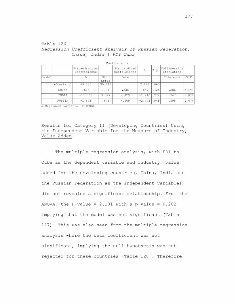
277

Table 126 Regression Coefficient Analysis of Russian Federation,

China, India & FDI Cuba

Coefficients Unstandardized

Coefficients Standardized

Coefficientst Sig. Collinearity

Statistics

Model B Std. Error

Beta Tolerance VIF

1 (Constant) 69.330 30.440 2.278 .063

CHINA .618 .721 .335 .857 .425 .286 3.497

INDIA -11.366 9.397 -.429 -1.210 .272 .347 2.878

RUSSIA -1.673 .676 -.669 -2.474 .048 .598 1.674

a Dependent Variable: FDICUBA

Results for Category II (Developing Countries) Using the Independent Variable for the Measure of Industry, Value Added

The multiple regression analysis, with FDI to

Cuba as the dependent variable and Industry, value

added for the developing countries, China, India and

the Russian Federation as the independent variables,

did not revealed a significant relationship. From the

ANOVA, the F-value = 2.101 with a p-value = 0.202

implying that the model was not significant (Table

127). This was also seen from the multiple regression

analysis where the beta coefficient was not

significant, implying the null hypothesis was not

rejected for these countries (Table 128). Therefore,

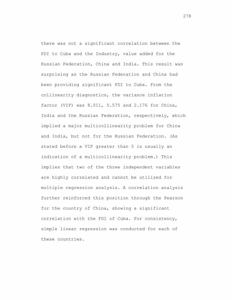
278

there was not a significant correlation between the

FDI to Cuba and the Industry, value added for the

Russian Federation, China and India. This result was

surprising as the Russian Federation and China had

been providing significant FDI to Cuba. From the

collinearity diagnostics, the variance inflation

factor (VIF) was 8.011, 5.575 and 2.176 for China,

India and the Russian Federation, respectively, which

implied a major multicollinearity problem for China

and India, but not for the Russian Federation. (As

stated before a VIF greater than 5 is usually an

indication of a multicollinearity problem.) This

implies that two of the three independent variables

are highly correlated and cannot be utilized for

multiple regression analysis. A correlation analysis

further reinforced this position through the Pearson

for the country of China, showing a significant

correlation with the FDI of Cuba. For consistency,

simple linear regression was conducted for each of

these countries.

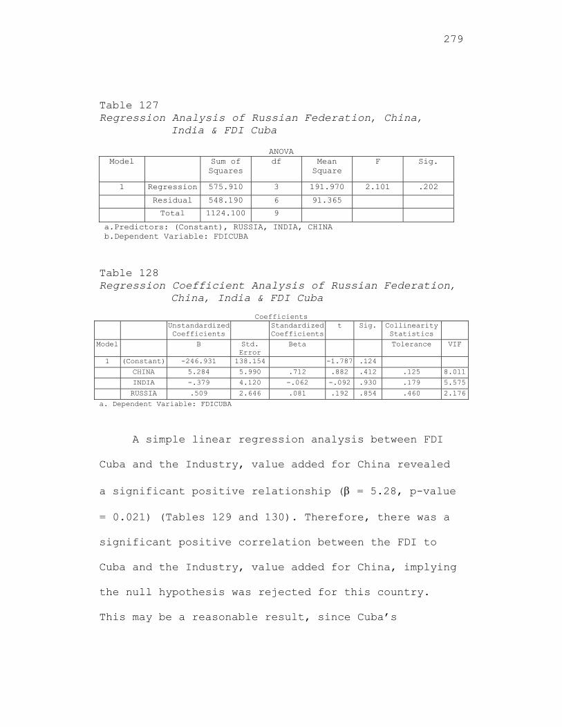
279

Table 127 Regression Analysis of Russian Federation, China,

India & FDI Cuba

ANOVA Model Sum of

Squares df Mean

Square F Sig.

1 Regression 575.910 3 191.970 2.101 .202

Residual 548.190 6 91.365

Total 1124.100 9

a.Predictors: (Constant), RUSSIA, INDIA, CHINA b.Dependent Variable: FDICUBA

Table 128 Regression Coefficient Analysis of Russian Federation,

China, India & FDI Cuba

Coefficients Unstandardized

Coefficients Standardized

Coefficientst Sig. Collinearity

Statistics

Model B Std. Error

Beta Tolerance VIF

1 (Constant) -246.931 138.154 -1.787 .124

CHINA 5.284 5.990 .712 .882 .412 .125 8.011

INDIA -.379 4.120 -.062 -.092 .930 .179 5.575

RUSSIA .509 2.646 .081 .192 .854 .460 2.176

a. Dependent Variable: FDICUBA

A simple linear regression analysis between FDI

Cuba and the Industry, value added for China revealed

a significant positive relationship ( = 5.28, p-value

= 0.021) (Tables 129 and 130). Therefore, there was a

significant positive correlation between the FDI to

Cuba and the Industry, value added for China, implying

the null hypothesis was rejected for this country.

This may be a reasonable result, since Cuba’s

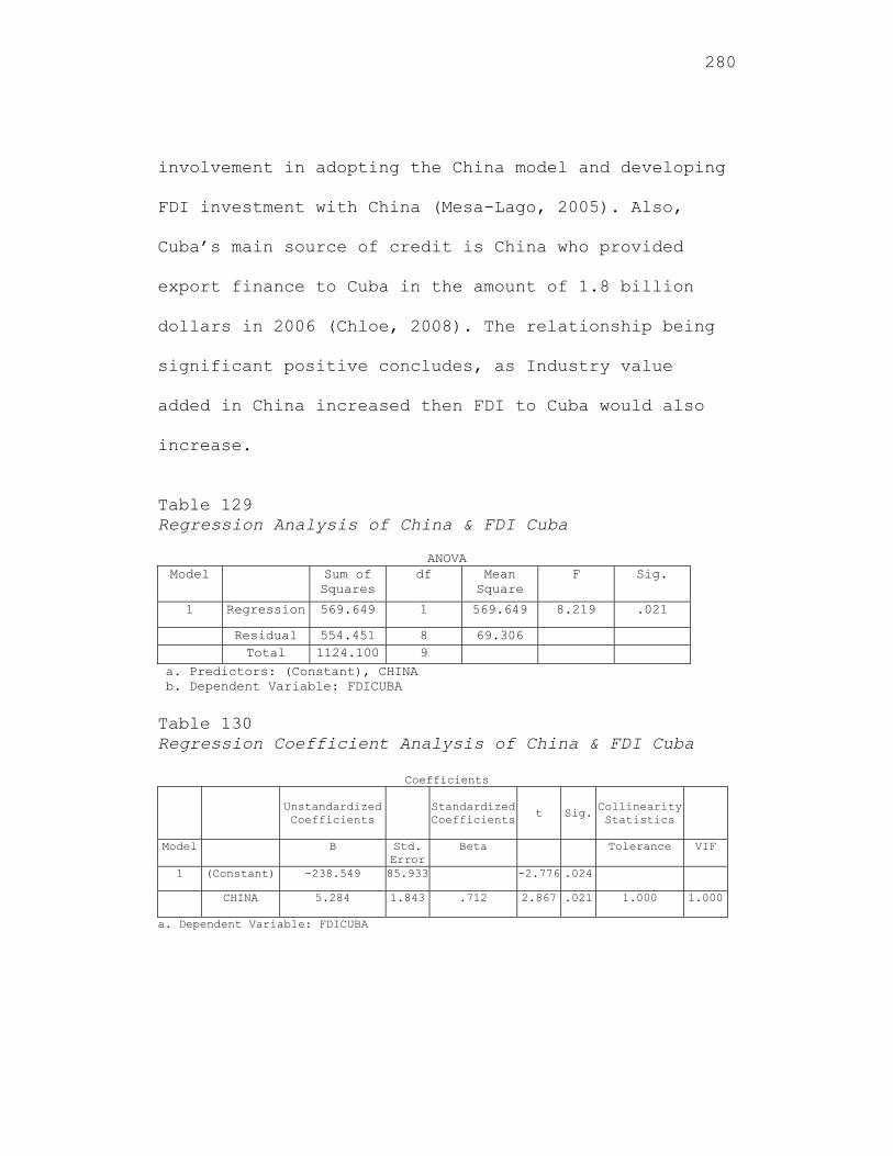
280

involvement in adopting the China model and developing

FDI investment with China (Mesa-Lago, 2005). Also,

Cuba’s main source of credit is China who provided

export finance to Cuba in the amount of 1.8 billion

dollars in 2006 (Chloe, 2008). The relationship being

significant positive concludes, as Industry value

added in China increased then FDI to Cuba would also

increase.

Table 129 Regression Analysis of China & FDI Cuba

ANOVA Model Sum of

Squares df Mean

Square F Sig.

1 Regression 569.649 1 569.649 8.219 .021

Residual 554.451 8 69.306 Total 1124.100 9

a. Predictors: (Constant), CHINA b. Dependent Variable: FDICUBA

Table 130 Regression Coefficient Analysis of China & FDI Cuba

Coefficients

Unstandardized Coefficients

Standardized Coefficients

t Sig. Collinearity Statistics

Model B Std. Error

Beta Tolerance VIF

1 (Constant) -238.549 85.933 -2.776 .024

CHINA 5.284 1.843 .712 2.867 .021 1.000 1.000

a. Dependent Variable: FDICUBA

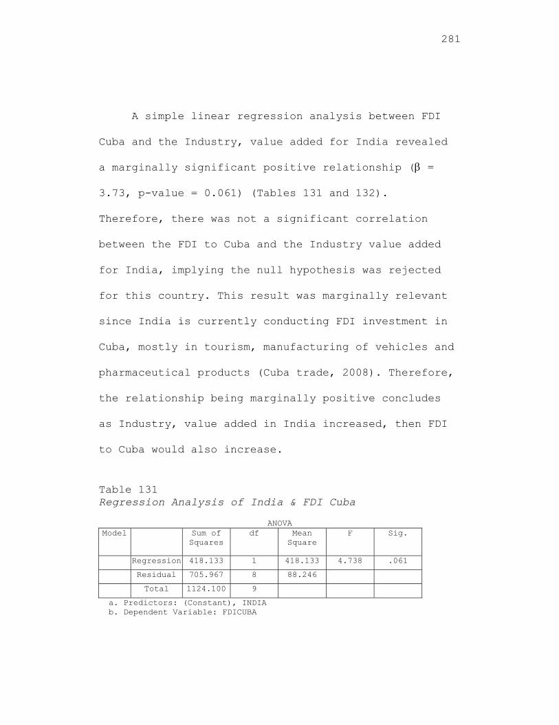
281

A simple linear regression analysis between FDI

Cuba and the Industry, value added for India revealed

a marginally significant positive relationship ( =

3.73, p-value = 0.061) (Tables 131 and 132).

Therefore, there was not a significant correlation

between the FDI to Cuba and the Industry value added

for India, implying the null hypothesis was rejected

for this country. This result was marginally relevant

since India is currently conducting FDI investment in

Cuba, mostly in tourism, manufacturing of vehicles and

pharmaceutical products (Cuba trade, 2008). Therefore,

the relationship being marginally positive concludes

as Industry, value added in India increased, then FDI

to Cuba would also increase.

Table 131 Regression Analysis of India & FDI Cuba

ANOVA Model Sum of

Squares df Mean

Square F Sig.

Regression 418.133 1 418.133 4.738 .061

Residual 705.967 8 88.246

Total 1124.100 9

a. Predictors: (Constant), INDIA b. Dependent Variable: FDICUBA

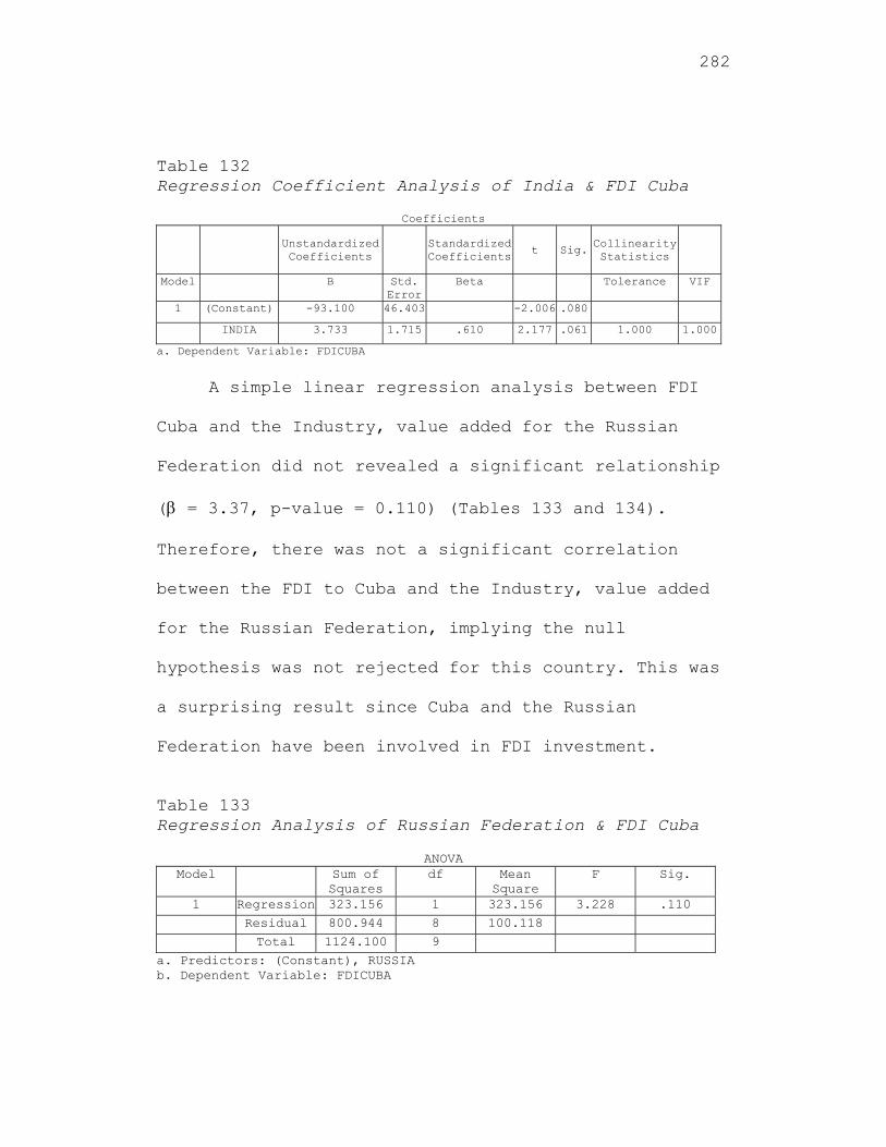
282

Table 132 Regression Coefficient Analysis of India & FDI Cuba

Coefficients

Unstandardized Coefficients

Standardized Coefficients t Sig.

Collinearity Statistics

Model B Std. Error

Beta Tolerance VIF

1 (Constant) -93.100 46.403 -2.006 .080

INDIA 3.733 1.715 .610 2.177 .061 1.000 1.000

a. Dependent Variable: FDICUBA

A simple linear regression analysis between FDI

Cuba and the Industry, value added for the Russian

Federation did not revealed a significant relationship

( = 3.37, p-value = 0.110) (Tables 133 and 134).

Therefore, there was not a significant correlation

between the FDI to Cuba and the Industry, value added

for the Russian Federation, implying the null

hypothesis was not rejected for this country. This was

a surprising result since Cuba and the Russian

Federation have been involved in FDI investment.

Table 133 Regression Analysis of Russian Federation & FDI Cuba

ANOVA Model Sum of

Squares df Mean

Square F Sig.

1 Regression 323.156 1 323.156 3.228 .110

Residual 800.944 8 100.118

Total 1124.100 9

a. Predictors: (Constant), RUSSIA b. Dependent Variable: FDICUBA

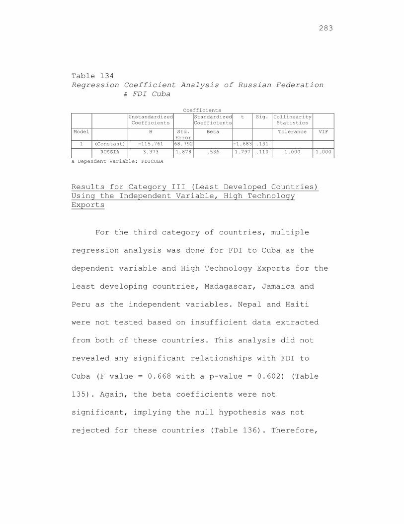
283

Table 134 Regression Coefficient Analysis of Russian Federation

& FDI Cuba

Coefficients Unstandardized

Coefficients Standardized

Coefficientst Sig. Collinearity

Statistics

Model B Std. Error

Beta Tolerance VIF

1 (Constant) -115.761 68.792 -1.683 .131

RUSSIA 3.373 1.878 .536 1.797 .110 1.000 1.000

a Dependent Variable: FDICUBA

Results for Category III (Least Developed Countries) Using the Independent Variable, High Technology Exports

For the third category of countries, multiple

regression analysis was done for FDI to Cuba as the

dependent variable and High Technology Exports for the

least developing countries, Madagascar, Jamaica and

Peru as the independent variables. Nepal and Haiti

were not tested based on insufficient data extracted

from both of these countries. This analysis did not

revealed any significant relationships with FDI to

Cuba (F value = 0.668 with a p-value = 0.602) (Table

135). Again, the beta coefficients were not

significant, implying the null hypothesis was not

rejected for these countries (Table 136). Therefore,

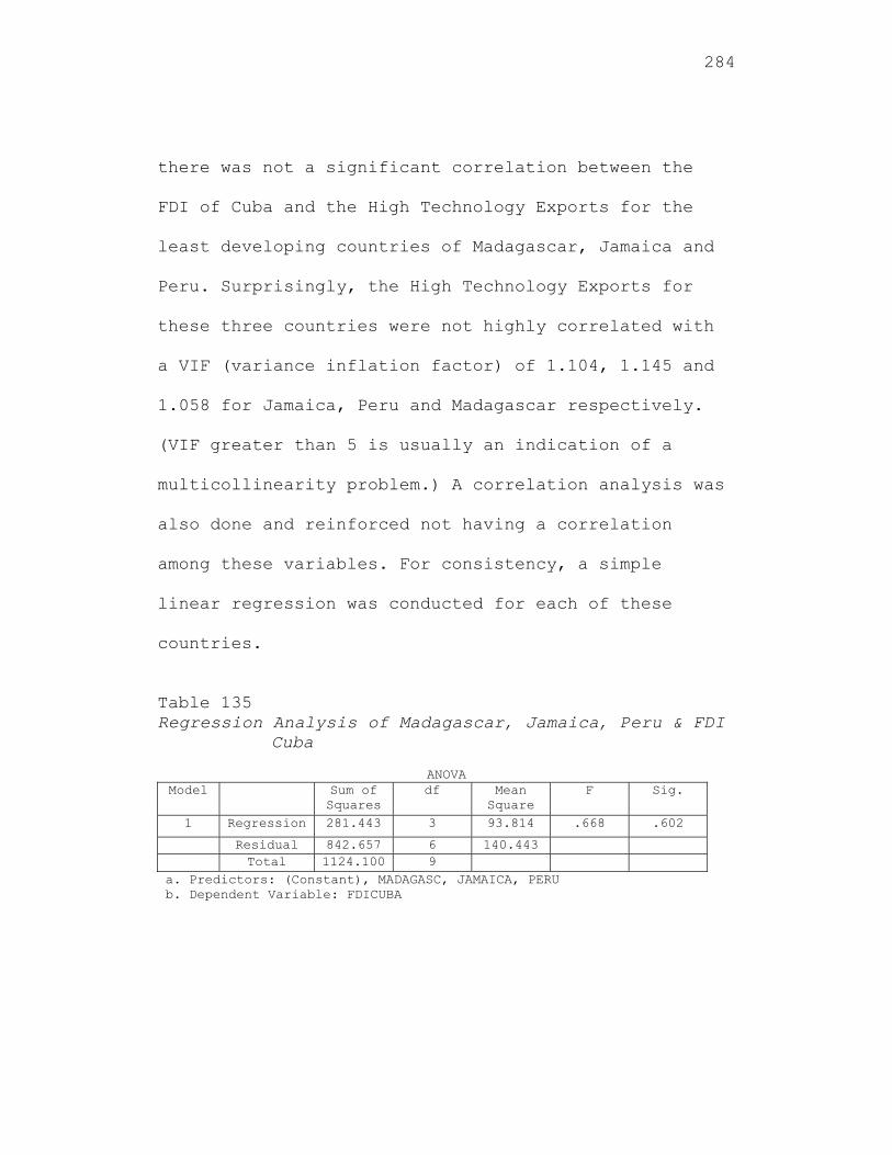
284

there was not a significant correlation between the

FDI of Cuba and the High Technology Exports for the

least developing countries of Madagascar, Jamaica and

Peru. Surprisingly, the High Technology Exports for

these three countries were not highly correlated with

a VIF (variance inflation factor) of 1.104, 1.145 and

1.058 for Jamaica, Peru and Madagascar respectively.

(VIF greater than 5 is usually an indication of a

multicollinearity problem.) A correlation analysis was

also done and reinforced not having a correlation

among these variables. For consistency, a simple

linear regression was conducted for each of these

countries.

Table 135 Regression Analysis of Madagascar, Jamaica, Peru & FDI

Cuba

ANOVA Model Sum of

Squares df Mean

Square F Sig.

1 Regression 281.443 3 93.814 .668 .602

Residual 842.657 6 140.443 Total 1124.100 9

a. Predictors: (Constant), MADAGASC, JAMAICA, PERU b. Dependent Variable: FDICUBA

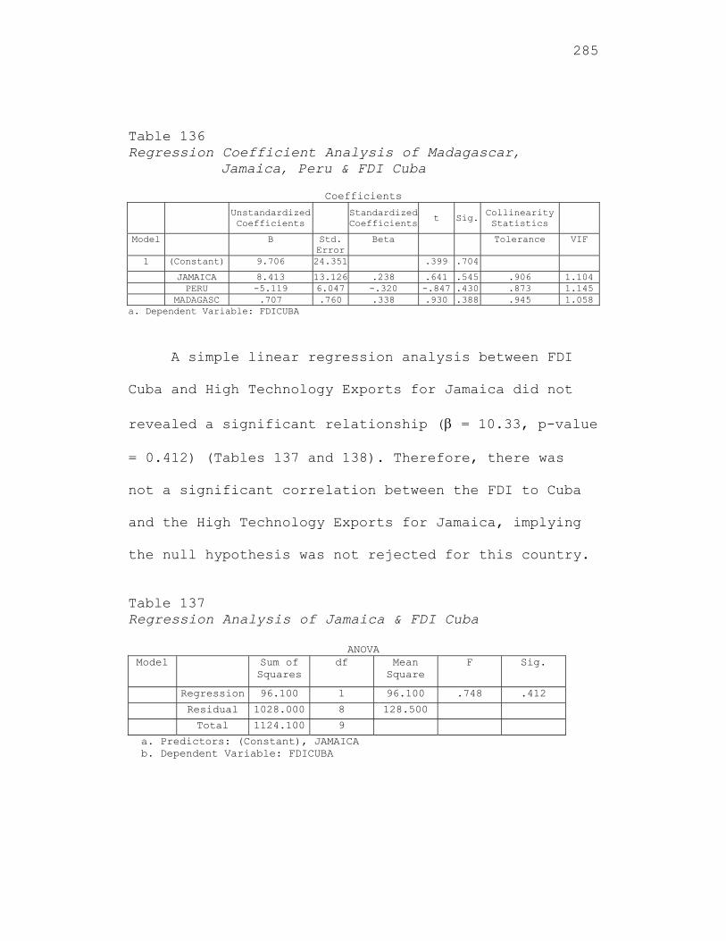
285

Table 136 Regression Coefficient Analysis of Madagascar,

Jamaica, Peru & FDI Cuba

Coefficients Unstandardized

Coefficients Standardized Coefficients t Sig.

Collinearity Statistics

Model B Std. Error

Beta Tolerance VIF

1 (Constant) 9.706 24.351 .399 .704

JAMAICA 8.413 13.126 .238 .641 .545 .906 1.104 PERU -5.119 6.047 -.320 -.847 .430 .873 1.145 MADAGASC .707 .760 .338 .930 .388 .945 1.058

a. Dependent Variable: FDICUBA

A simple linear regression analysis between FDI

Cuba and High Technology Exports for Jamaica did not

revealed a significant relationship ( = 10.33, p-value

= 0.412) (Tables 137 and 138). Therefore, there was

not a significant correlation between the FDI to Cuba

and the High Technology Exports for Jamaica, implying

the null hypothesis was not rejected for this country.

Table 137 Regression Analysis of Jamaica & FDI Cuba

ANOVA Model Sum of

Squares df Mean

Square F Sig.

Regression 96.100 1 96.100 .748 .412

Residual 1028.000 8 128.500

Total 1124.100 9

a. Predictors: (Constant), JAMAICA b. Dependent Variable: FDICUBA

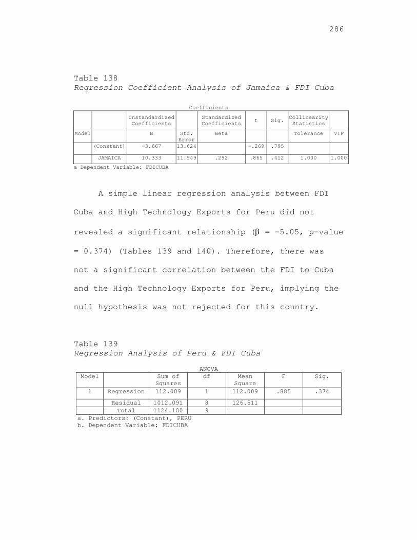
286

Table 138 Regression Coefficient Analysis of Jamaica & FDI Cuba

Coefficients

Unstandardized Coefficients

Standardized Coefficients

t Sig. Collinearity Statistics

Model B Std. Error

Beta Tolerance VIF

(Constant) -3.667 13.624 -.269 .795

JAMAICA 10.333 11.949 .292 .865 .412 1.000 1.000

a Dependent Variable: FDICUBA

A simple linear regression analysis between FDI

Cuba and High Technology Exports for Peru did not

revealed a significant relationship ( = -5.05, p-value

= 0.374) (Tables 139 and 140). Therefore, there was

not a significant correlation between the FDI to Cuba

and the High Technology Exports for Peru, implying the

null hypothesis was not rejected for this country.

Table 139 Regression Analysis of Peru & FDI Cuba

ANOVA Model Sum of

Squares df Mean

Square F Sig.

1 Regression 112.009 1 112.009 .885 .374

Residual 1012.091 8 126.511 Total 1124.100 9

a. Predictors: (Constant), PERU b. Dependent Variable: FDICUBA

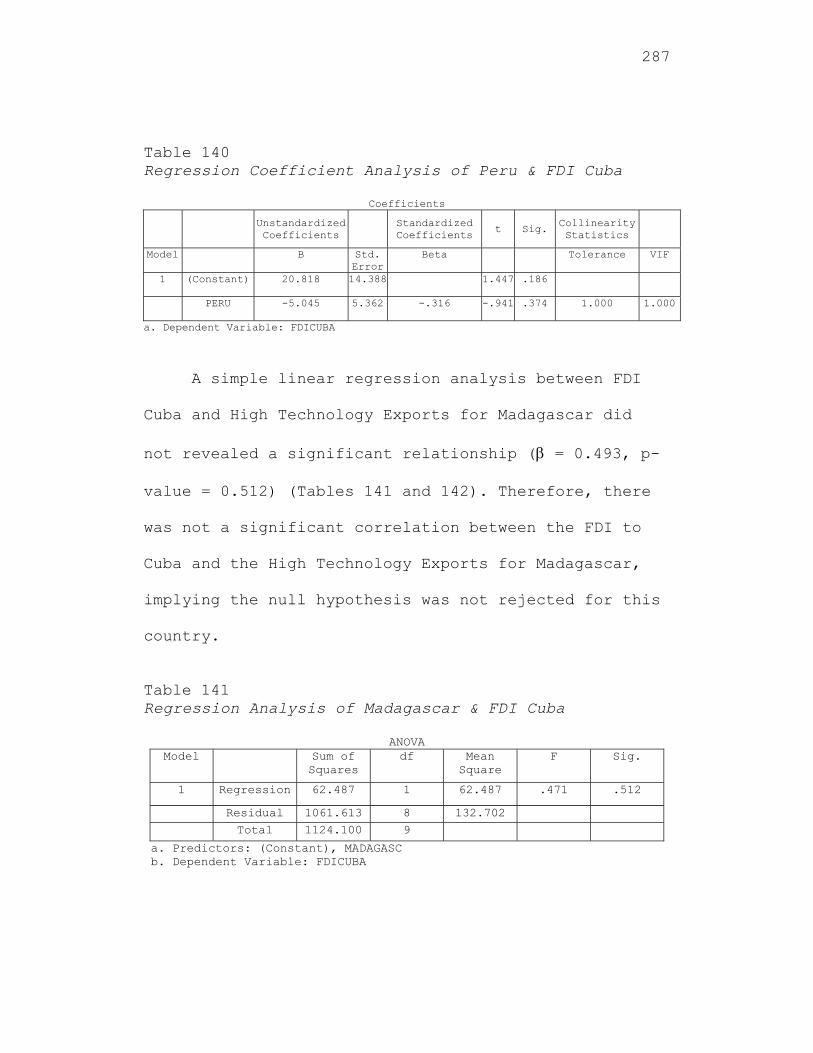
287

Table 140 Regression Coefficient Analysis of Peru & FDI Cuba

Coefficients

Unstandardized Coefficients

Standardized Coefficients

t Sig. Collinearity Statistics

Model B Std. Error

Beta Tolerance VIF

1 (Constant) 20.818 14.388 1.447 .186

PERU -5.045 5.362 -.316 -.941 .374 1.000 1.000

a. Dependent Variable: FDICUBA

A simple linear regression analysis between FDI

Cuba and High Technology Exports for Madagascar did

not revealed a significant relationship ( = 0.493, p-

value = 0.512) (Tables 141 and 142). Therefore, there

was not a significant correlation between the FDI to

Cuba and the High Technology Exports for Madagascar,

implying the null hypothesis was not rejected for this

country.

Table 141 Regression Analysis of Madagascar & FDI Cuba

ANOVA Model Sum of

Squares df Mean

Square F Sig.

1 Regression 62.487 1 62.487 .471 .512

Residual 1061.613 8 132.702

Total 1124.100 9

a. Predictors: (Constant), MADAGASC b. Dependent Variable: FDICUBA

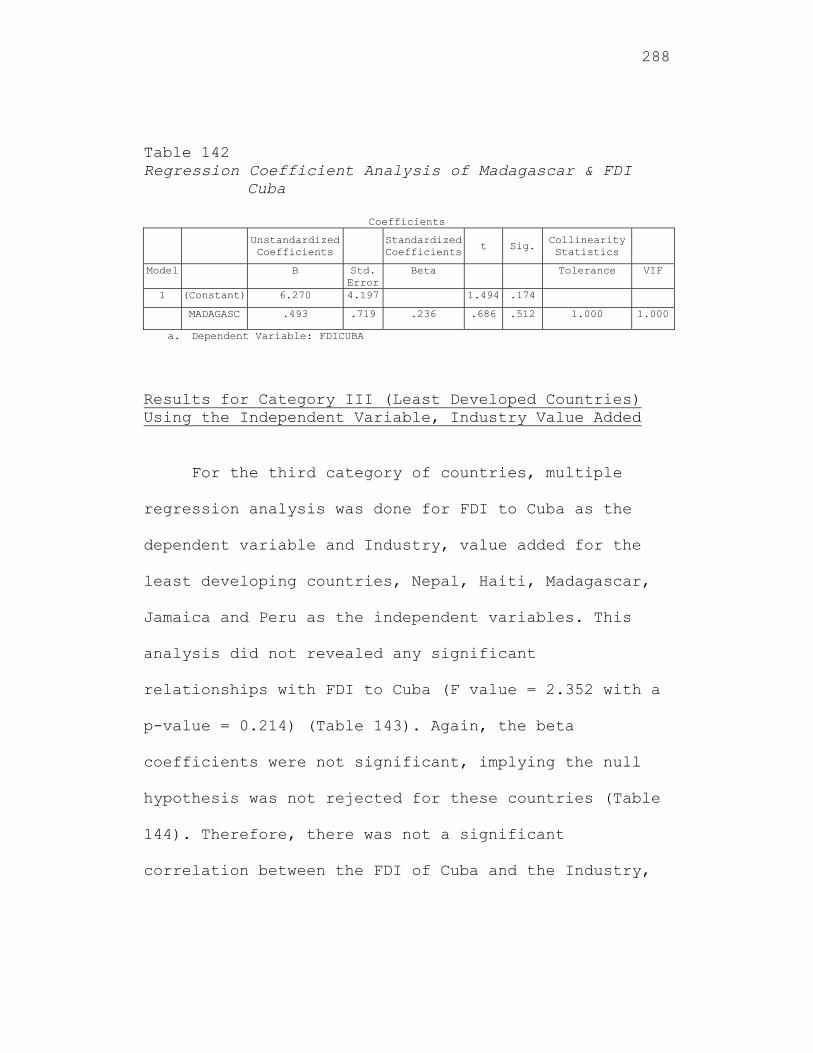
288

Table 142 Regression Coefficient Analysis of Madagascar & FDI

Cuba

Coefficients Unstandardized

Coefficients Standardized Coefficients t Sig.

Collinearity Statistics

Model B Std. Error

Beta Tolerance VIF

1 (Constant) 6.270 4.197 1.494 .174

MADAGASC .493 .719 .236 .686 .512 1.000 1.000

a. Dependent Variable: FDICUBA

Results for Category III (Least Developed Countries) Using the Independent Variable, Industry Value Added

For the third category of countries, multiple

regression analysis was done for FDI to Cuba as the

dependent variable and Industry, value added for the

least developing countries, Nepal, Haiti, Madagascar,

Jamaica and Peru as the independent variables. This

analysis did not revealed any significant

relationships with FDI to Cuba (F value = 2.352 with a

p-value = 0.214) (Table 143). Again, the beta

coefficients were not significant, implying the null

hypothesis was not rejected for these countries (Table

144). Therefore, there was not a significant

correlation between the FDI of Cuba and the Industry,

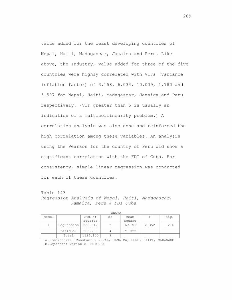
289

value added for the least developing countries of

Nepal, Haiti, Madagascar, Jamaica and Peru. Like

above, the Industry, value added for three of the five

countries were highly correlated with VIFs (variance

inflation factor) of 3.158, 6.034, 10.039, 1.780 and

5.507 for Nepal, Haiti, Madagascar, Jamaica and Peru

respectively. (VIF greater than 5 is usually an

indication of a multicollinearity problem.) A

correlation analysis was also done and reinforced the

high correlation among these variables. An analysis

using the Pearson for the country of Peru did show a

significant correlation with the FDI of Cuba. For

consistency, simple linear regression was conducted

for each of these countries.

Table 143 Regression Analysis of Nepal, Haiti, Madagascar,

Jamaica, Peru & FDI Cuba

ANOVA Model Sum of

Squares df Mean

Square F Sig.

1 Regression 838.812 5 167.762 2.352 .214

Residual 285.288 4 71.322 Total 1124.100 9

a.Predictors: (Constant), NEPAL, JAMAICA, PERU, HAITI, MADAGASC b.Dependent Variable: FDICUBA

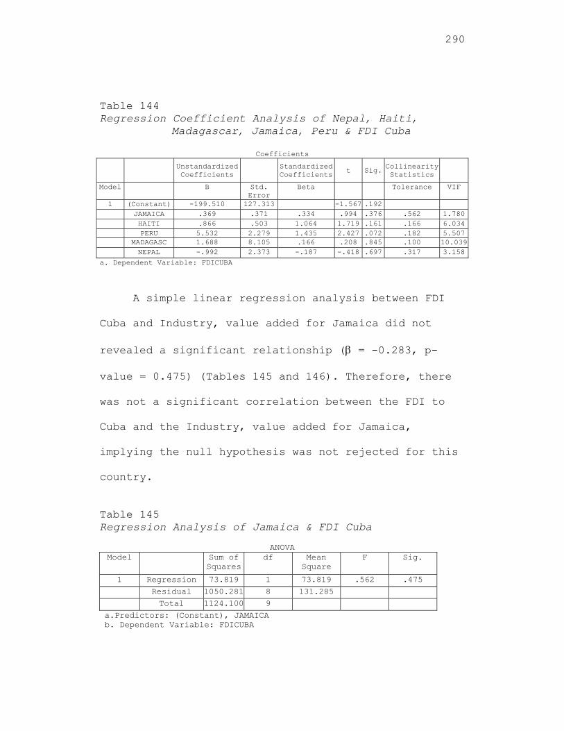
290

Table 144 Regression Coefficient Analysis of Nepal, Haiti,

Madagascar, Jamaica, Peru & FDI Cuba

Coefficients Unstandardized

Coefficients Standardized

Coefficientst Sig. Collinearity

Statistics

Model B Std. Error

Beta Tolerance VIF

1 (Constant) -199.510 127.313 -1.567 .192 JAMAICA .369 .371 .334 .994 .376 .562 1.780 HAITI .866 .503 1.064 1.719 .161 .166 6.034 PERU 5.532 2.279 1.435 2.427 .072 .182 5.507 MADAGASC 1.688 8.105 .166 .208 .845 .100 10.039 NEPAL -.992 2.373 -.187 -.418 .697 .317 3.158

a. Dependent Variable: FDICUBA

A simple linear regression analysis between FDI

Cuba and Industry, value added for Jamaica did not

revealed a significant relationship ( = -0.283, p-

value = 0.475) (Tables 145 and 146). Therefore, there

was not a significant correlation between the FDI to

Cuba and the Industry, value added for Jamaica,

implying the null hypothesis was not rejected for this

country.

Table 145 Regression Analysis of Jamaica & FDI Cuba

ANOVA

Model Sum of Squares

df Mean Square

F Sig.

1 Regression 73.819 1 73.819 .562 .475

Residual 1050.281 8 131.285

Total 1124.100 9

a.Predictors: (Constant), JAMAICA b. Dependent Variable: FDICUBA

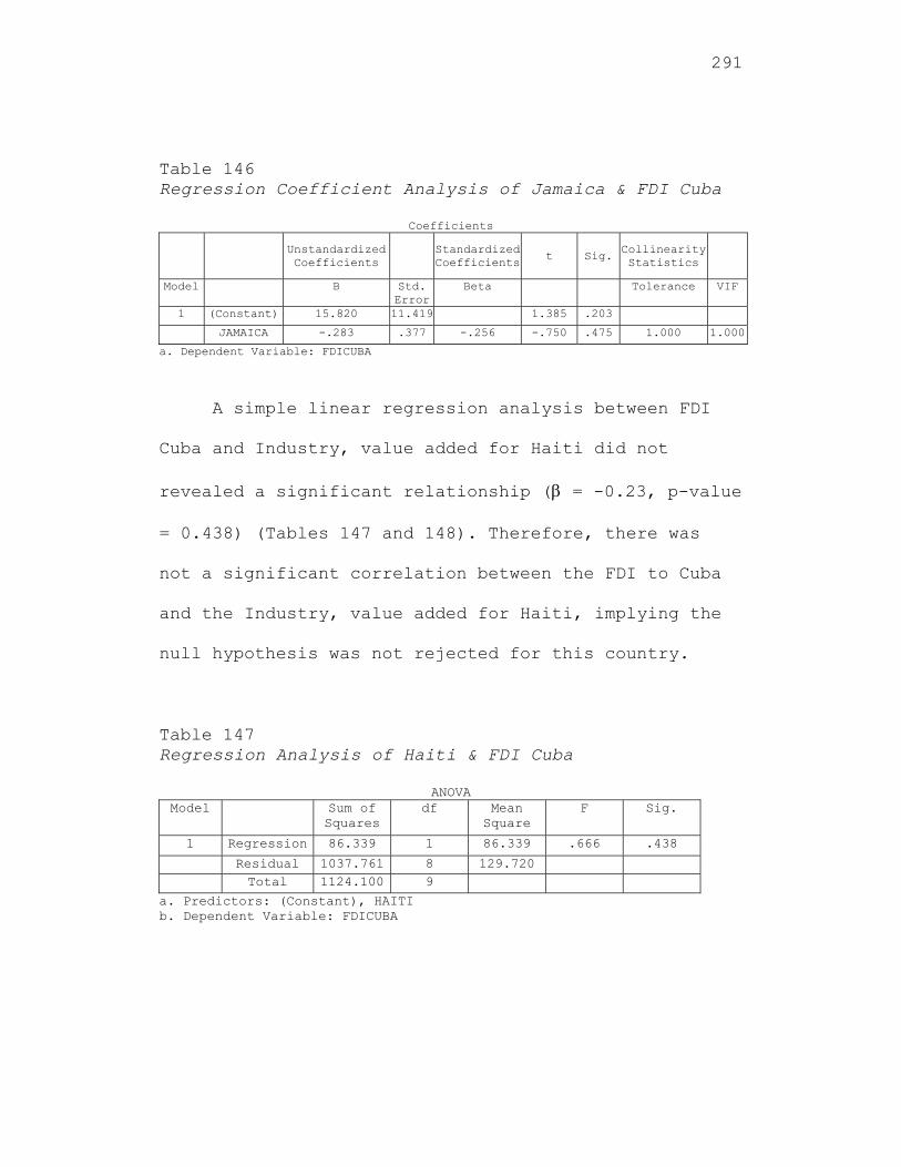
291

Table 146 Regression Coefficient Analysis of Jamaica & FDI Cuba

Coefficients

Unstandardized Coefficients

Standardized Coefficients t Sig.

Collinearity Statistics

Model B Std. Error

Beta Tolerance VIF

1 (Constant) 15.820 11.419 1.385 .203

JAMAICA -.283 .377 -.256 -.750 .475 1.000 1.000

a. Dependent Variable: FDICUBA

A simple linear regression analysis between FDI

Cuba and Industry, value added for Haiti did not

revealed a significant relationship ( = -0.23, p-value

= 0.438) (Tables 147 and 148). Therefore, there was

not a significant correlation between the FDI to Cuba

and the Industry, value added for Haiti, implying the

null hypothesis was not rejected for this country.

Table 147 Regression Analysis of Haiti & FDI Cuba

ANOVA Model Sum of

Squares df Mean

Square F Sig.

1 Regression 86.339 1 86.339 .666 .438

Residual 1037.761 8 129.720 Total 1124.100 9

a. Predictors: (Constant), HAITI b. Dependent Variable: FDICUBA

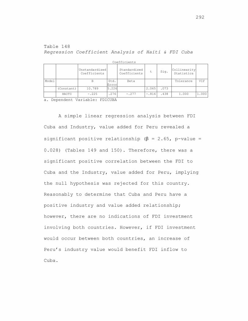
292

Table 148 Regression Coefficient Analysis of Haiti & FDI Cuba

Coefficients

Unstandardized Coefficients

Standardized Coefficients

t Sig. Collinearity Statistics

Model B Std. Error

Beta Tolerance VIF

(Constant) 10.789 5.226 2.065 .073

HAITI -.225 .276 -.277 -.816 .438 1.000 1.000

a. Dependent Variable: FDICUBA

A simple linear regression analysis between FDI

Cuba and Industry, value added for Peru revealed a

significant positive relationship ( = 2.65, p-value =

0.028) (Tables 149 and 150). Therefore, there was a

significant positive correlation between the FDI to

Cuba and the Industry, value added for Peru, implying

the null hypothesis was rejected for this country.

Reasonably to determine that Cuba and Peru have a

positive industry and value added relationship;

however, there are no indications of FDI investment

involving both countries. However, if FDI investment

would occur between both countries, an increase of

Peru’s industry value would benefit FDI inflow to

Cuba.

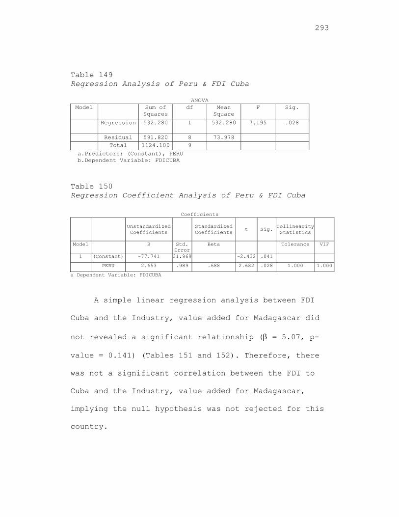
293

Table 149 Regression Analysis of Peru & FDI Cuba

ANOVA Model Sum of

Squares df Mean

Square F Sig.

Regression 532.280 1 532.280 7.195 .028

Residual 591.820 8 73.978 Total 1124.100 9

a.Predictors: (Constant), PERU b.Dependent Variable: FDICUBA

Table 150 Regression Coefficient Analysis of Peru & FDI Cuba

Coefficients

Unstandardized Coefficients

Standardized Coefficients

t Sig. Collinearity Statistics

Model B Std. Error

Beta Tolerance VIF

1 (Constant) -77.741 31.969 -2.432 .041

PERU 2.653 .989 .688 2.682 .028 1.000 1.000

a Dependent Variable: FDICUBA

A simple linear regression analysis between FDI

Cuba and the Industry, value added for Madagascar did

not revealed a significant relationship ( = 5.07, p-

value = 0.141) (Tables 151 and 152). Therefore, there

was not a significant correlation between the FDI to

Cuba and the Industry, value added for Madagascar,

implying the null hypothesis was not rejected for this

country.

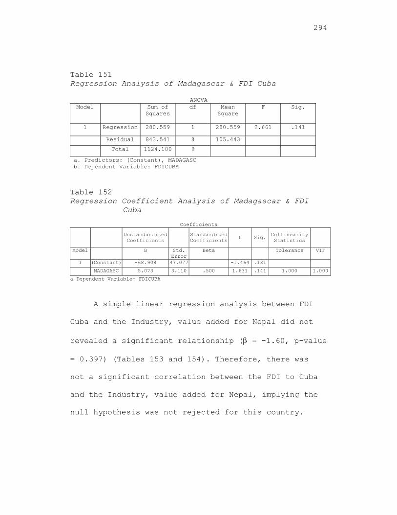
294

Table 151 Regression Analysis of Madagascar & FDI Cuba

ANOVA Model Sum of

Squares df Mean

Square F Sig.

1 Regression 280.559 1 280.559 2.661 .141

Residual 843.541 8 105.443

Total 1124.100 9

a. Predictors: (Constant), MADAGASC b. Dependent Variable: FDICUBA

Table 152 Regression Coefficient Analysis of Madagascar & FDI

Cuba

Coefficients

Unstandardized Coefficients

Standardized Coefficients

t Sig. Collinearity Statistics

Model B Std. Error

Beta Tolerance VIF

1 (Constant) -68.908 47.077 -1.464 .181

MADAGASC 5.073 3.110 .500 1.631 .141 1.000 1.000

a Dependent Variable: FDICUBA

A simple linear regression analysis between FDI

Cuba and the Industry, value added for Nepal did not

revealed a significant relationship ( = -1.60, p-value

= 0.397) (Tables 153 and 154). Therefore, there was

not a significant correlation between the FDI to Cuba

and the Industry, value added for Nepal, implying the

null hypothesis was not rejected for this country.

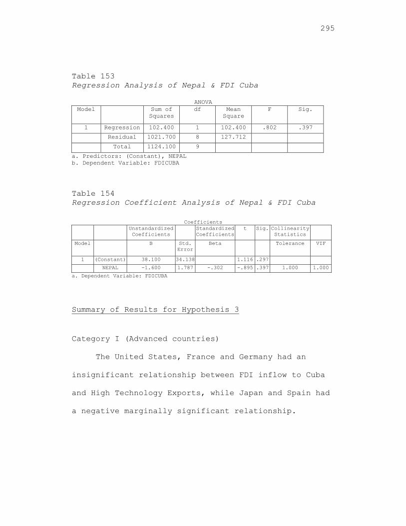
295

Table 153 Regression Analysis of Nepal & FDI Cuba

ANOVA Model Sum of

Squares df Mean

Square F Sig.

1 Regression 102.400 1 102.400 .802 .397

Residual 1021.700 8 127.712

Total 1124.100 9

a. Predictors: (Constant), NEPAL b. Dependent Variable: FDICUBA Table 154 Regression Coefficient Analysis of Nepal & FDI Cuba

Coefficients

Unstandardized Coefficients

Standardized Coefficients

t Sig. Collinearity Statistics

Model B Std. Error

Beta Tolerance VIF

1 (Constant) 38.100 34.138 1.116 .297

NEPAL -1.600 1.787 -.302 -.895 .397 1.000 1.000

a. Dependent Variable: FDICUBA

Summary of Results for Hypothesis 3

Category I (Advanced countries)

The United States, France and Germany had an

insignificant relationship between FDI inflow to Cuba

and High Technology Exports, while Japan and Spain had

a negative marginally significant relationship.

296

Significant positive relationship existed between

FDI inflow to Cuba and the Industry, value added for

Spain. Insignificant results were found for the United

States, Japan, France and Germany.

Category II (Developing Countries)

Significant positive correlation existed between

FDI inflow to Cuba and High Technology Exports for

China, India and the Russian Federation.

Significant positive correlation existed between

FDI inflow to Cuba and Industry, value added for

China. Insignificant results were found for the

Russian Federation while India, showed a marginal

positive correlation result.

Category III (Least Developing Countries)

Insignificant relationship existed between FDI

inflow to Cuba and High Technology Exports for

Jamaica, Peru and Madagascar. Nepal and Haiti was not

tested based on insufficient data.

297

Significant positive correlation existed between

FDI inflow to Cuba and Industry, value added for Peru.

Insignificant results were found for Jamaica, Haiti,

Madagascar and Nepal.

Results for Hypothesis 4

FDI to Cuba was the dependent variable. For the

advanced countries, the independent variables were

Human Capital for the United States, Japan, Germany,

France and Spain (Sawalha, 2007). The independent

variables for the developing countries were Human

Capital for China, India and the Russian Federation

(Sawalha, 2007). The independent variables for the

Least Developed Countries (LCD’s) were Human Capital

for Jamaica, Haiti, Peru, Madagascar and Nepal. The

Republic of Cuba’s Human Capital was not included in

the model as there were only three data points. The

Human Capital hypothesis included two variables, School

Enrollment (measured by tertiary education as a

percentage of gross school enrollments) and Total

298

Unemployment (measured as a percentage of the total

labor force).

The fourth hypothesis to be tested is:

Hypothesis H04: The level of contribution of FDI

inflow to Cuba is not significantly related to

Human Capital for the three groups of

countries.

Hypothesis HA4: The level of contribution of FDI

inflow to Cuba is significantly related to

Human Capital for the three groups of

countries.

The multiple regression models to test Hypothesis 4

are listed below.

Category I (Advanced Countries)

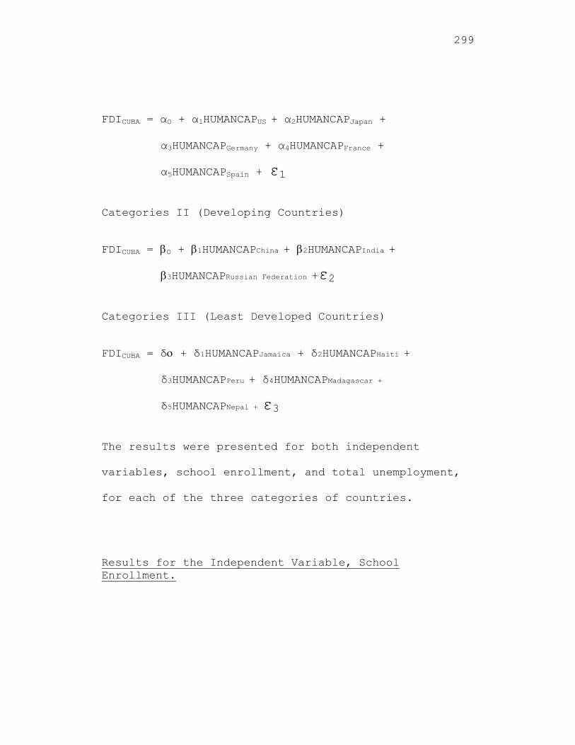
299

FDICUBA = αO + α1HUMANCAPUS + α2HUMANCAPJapan +

α3HUMANCAPGermany + α4HUMANCAPFrance +

α5HUMANCAPSpain + ε1

Categories II (Developing Countries)

FDICUBA = O + 1HUMANCAPChina + 2HUMANCAPIndia +

3HUMANCAPRussian Federation +ε2

Categories III (Least Developed Countries)

FDICUBA = δ + δ1HUMANCAPJamaica + δ2HUMANCAPHaiti +

δ3HUMANCAPPeru + δ4HUMANCAPMadagascar +

δ5HUMANCAPNepal + ε3

The results were presented for both independent

variables, school enrollment, and total unemployment,

for each of the three categories of countries.

Results for the Independent Variable, School Enrollment.

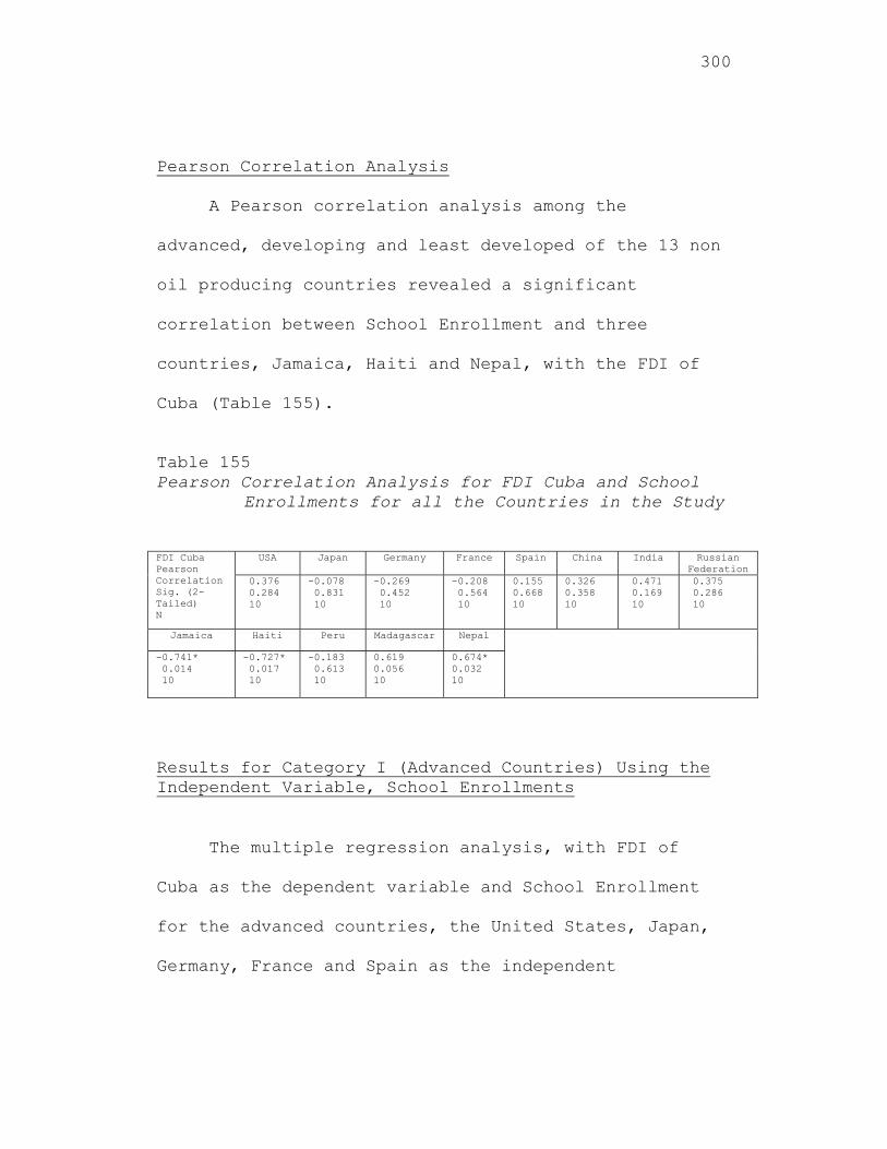
300

Pearson Correlation Analysis

A Pearson correlation analysis among the

advanced, developing and least developed of the 13 non

oil producing countries revealed a significant

correlation between School Enrollment and three

countries, Jamaica, Haiti and Nepal, with the FDI of

Cuba (Table 155).

Table 155 Pearson Correlation Analysis for FDI Cuba and School

Enrollments for all the Countries in the Study FDI Cuba Pearson Correlation Sig. (2-Tailed) N

USA Japan Germany France Spain China India Russian Federation

0.376 0.284 10

-0.078 0.831 10

-0.269 0.452 10

-0.208 0.564 10

0.155 0.668 10

0.326 0.358 10

0.471 0.169 10

0.375 0.286 10

Jamaica Haiti Peru Madagascar Nepal

-0.741* 0.014 10

-0.727* 0.017 10

-0.183 0.613 10

0.619 0.056 10

0.674* 0.032 10

Results for Category I (Advanced Countries) Using the Independent Variable, School Enrollments

The multiple regression analysis, with FDI of

Cuba as the dependent variable and School Enrollment

for the advanced countries, the United States, Japan,

Germany, France and Spain as the independent

301

variables, did not revealed any significant

relationships. From the ANOVA, the F-value = 2.477

with a p-value = 0.200 implying that the model was not

significant (Table 156). This was also seen from the

multiple regression analysis where the beta

coefficients were not significant, implying the null

hypothesis was not rejected for these countries (Table

157). Therefore, there was not a significant

correlation between the FDI of Cuba and School

Enrollment for these advanced countries, the United

States, Japan, Germany, France and Spain. From the

collinearity diagnostics, the variance inflation

factor (VIF) was 3.879, 347.642, 3.488, 182.569 and

58.624 for the United States, Japan, Germany, France

and Spain, respectively. (VIF greater than 5 is

usually an indication of a multicollinearity problem.)

This implies that there was a major multicollinearity

problem with the independent variables. A correlation

analysis further reinforced this position. Simple

linear regression was conducted for each of these

countries.

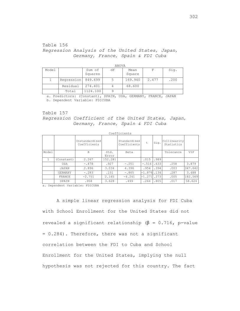
302

Table 156 Regression Analysis of the United States, Japan,

Germany, France, Spain & FDI Cuba

ANOVA Model Sum of

Squares df Mean

Square F Sig.

1 Regression 849.699 5 169.940 2.477 .200

Residual 274.401 4 68.600

Total 1124.100 9

a. Predictors: (Constant), SPAIN, USA, GERMANY, FRANCE, JAPAN b. Dependent Variable: FDICUBA

Table 157 Regression Coefficient of the United States, Japan,

Germany, France, Spain & FDI Cuba

Coefficients

Unstandardized Coefficients

Standardized Coefficients

t Sig.Collinearity Statistics

Model B Std. Error

Beta Tolerance VIF

1 (Constant) 2.267 152.281 .015 .989 USA -.478 .927 -.251 -.516 .633 .258 3.879 JAPAN 2.896 3.034 4.396 .954 .394 .003 347.642 GERMANY -.283 .151 -.865 -1.876 .134 .287 3.488 FRANCE -2.751 2.165 -4.241 -1.271 .273 .005 182.569 SPAIN .958 3.628 .499 .264 .805 .017 58.624

a. Dependent Variable: FDICUBA

A simple linear regression analysis for FDI Cuba

with School Enrollment for the United States did not

revealed a significant relationship ( = 0.716, p-value

= 0.284). Therefore, there was not a significant

correlation between the FDI to Cuba and School

Enrollment for the United States, implying the null

hypothesis was not rejected for this country. The fact

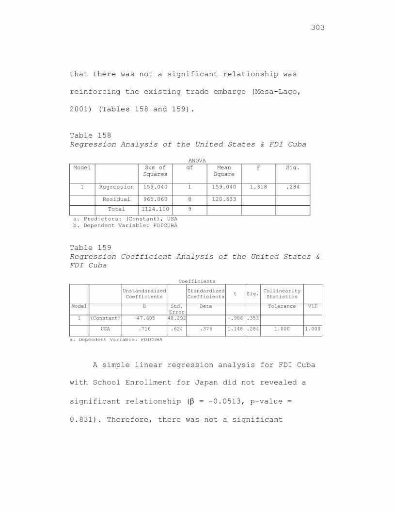
303

that there was not a significant relationship was

reinforcing the existing trade embargo (Mesa-Lago,

2001) (Tables 158 and 159).

Table 158 Regression Analysis of the United States & FDI Cuba

ANOVA Model Sum of

Squares df Mean

Square F Sig.

1 Regression 159.040 1 159.040 1.318 .284

Residual 965.060 8 120.633

Total 1124.100 9

a. Predictors: (Constant), USA b. Dependent Variable: FDICUBA Table 159 Regression Coefficient Analysis of the United States & FDI Cuba

Coefficients

Unstandardized Coefficients

Standardized Coefficients t Sig.

Collinearity Statistics

Model B Std. Error

Beta Tolerance VIF

1 (Constant) -47.605 48.292 -.986 .353

USA .716 .624 .376 1.148 .284 1.000 1.000

a. Dependent Variable: FDICUBA

A simple linear regression analysis for FDI Cuba

with School Enrollment for Japan did not revealed a

significant relationship ( = -0.0513, p-value =

0.831). Therefore, there was not a significant

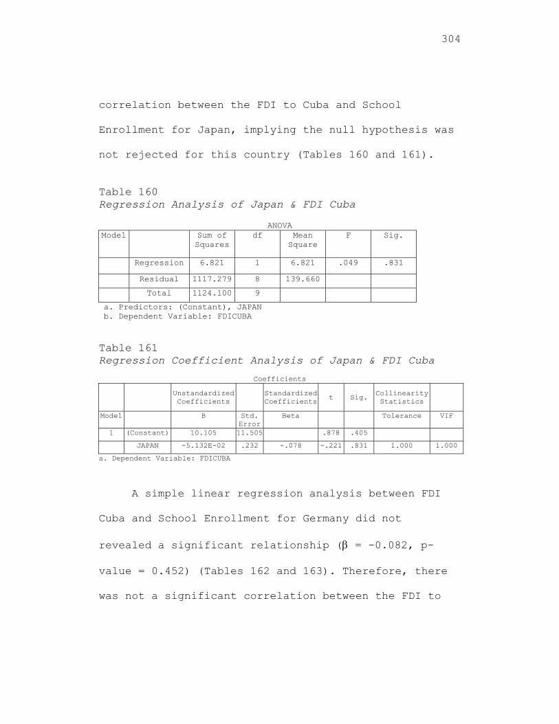
304

correlation between the FDI to Cuba and School

Enrollment for Japan, implying the null hypothesis was

not rejected for this country (Tables 160 and 161).

Table 160 Regression Analysis of Japan & FDI Cuba

ANOVA

Model Sum of Squares

df Mean Square

F Sig.

Regression 6.821 1 6.821 .049 .831

Residual 1117.279 8 139.660

Total 1124.100 9

a. Predictors: (Constant), JAPAN b. Dependent Variable: FDICUBA Table 161 Regression Coefficient Analysis of Japan & FDI Cuba

Coefficients

Unstandardized Coefficients

Standardized Coefficients

t Sig. Collinearity Statistics

Model B Std. Error

Beta Tolerance VIF

1 (Constant) 10.105 11.505 .878 .405

JAPAN -5.132E-02 .232 -.078 -.221 .831 1.000 1.000

a. Dependent Variable: FDICUBA

A simple linear regression analysis between FDI

Cuba and School Enrollment for Germany did not

revealed a significant relationship ( = -0.082, p-

value = 0.452) (Tables 162 and 163). Therefore, there

was not a significant correlation between the FDI to

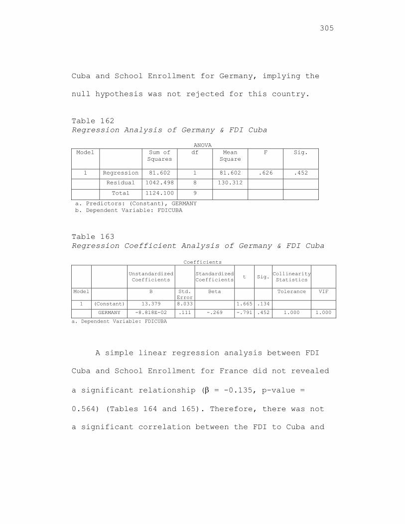
305

Cuba and School Enrollment for Germany, implying the

null hypothesis was not rejected for this country.

Table 162 Regression Analysis of Germany & FDI Cuba

ANOVA Model Sum of

Squares df Mean

Square F Sig.

1 Regression 81.602 1 81.602 .626 .452

Residual 1042.498 8 130.312

Total 1124.100 9

a. Predictors: (Constant), GERMANY b. Dependent Variable: FDICUBA

Table 163 Regression Coefficient Analysis of Germany & FDI Cuba

Coefficients

Unstandardized Coefficients

Standardized Coefficients t Sig.

Collinearity Statistics

Model B Std. Error

Beta Tolerance VIF

1 (Constant) 13.379 8.033 1.665 .134

GERMANY -8.818E-02 .111 -.269 -.791 .452 1.000 1.000

a. Dependent Variable: FDICUBA

A simple linear regression analysis between FDI

Cuba and School Enrollment for France did not revealed

a significant relationship ( = -0.135, p-value =

0.564) (Tables 164 and 165). Therefore, there was not

a significant correlation between the FDI to Cuba and

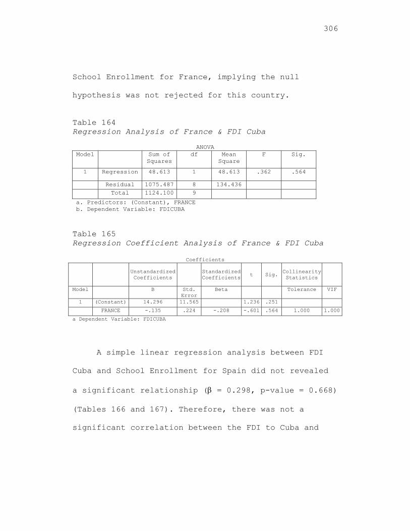
306

School Enrollment for France, implying the null

hypothesis was not rejected for this country.

Table 164 Regression Analysis of France & FDI Cuba

ANOVA Model Sum of

Squares df Mean

Square F Sig.

1 Regression 48.613 1 48.613 .362 .564

Residual 1075.487 8 134.436 Total 1124.100 9

a. Predictors: (Constant), FRANCE b. Dependent Variable: FDICUBA Table 165 Regression Coefficient Analysis of France & FDI Cuba

Coefficients

Unstandardized Coefficients

Standardized Coefficients t Sig.

Collinearity Statistics

Model B Std. Error

Beta Tolerance VIF

1 (Constant) 14.296 11.565 1.236 .251

FRANCE -.135 .224 -.208 -.601 .564 1.000 1.000

a Dependent Variable: FDICUBA

A simple linear regression analysis between FDI

Cuba and School Enrollment for Spain did not revealed

a significant relationship ( = 0.298, p-value = 0.668)

(Tables 166 and 167). Therefore, there was not a

significant correlation between the FDI to Cuba and

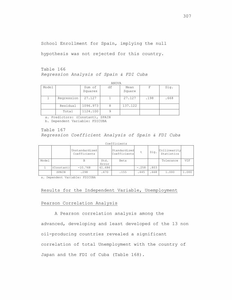
307

School Enrollment for Spain, implying the null

hypothesis was not rejected for this country.

Table 166 Regression Analysis of Spain & FDI Cuba

ANOVA Model Sum of

Squares df Mean

Square F Sig.

1 Regression 27.127 1 27.127 .198 .668

Residual 1096.973 8 137.122

Total 1124.100 9

a. Predictors: (Constant), SPAIN b. Dependent Variable: FDICUBA Table 167 Regression Coefficient Analysis of Spain & FDI Cuba

Coefficients

Unstandardized Coefficients

Standardized Coefficients t Sig.

Collinearity Statistics

Model B Std. Error

Beta Tolerance VIF

1 (Constant) -10.768 41.686 -.258 .803

SPAIN .298 .670 .155 .445 .668 1.000 1.000

a. Dependent Variable: FDICUBA

Results for the Independent Variable, Unemployment

Pearson Correlation Analysis

A Pearson correlation analysis among the

advanced, developing and least developed of the 13 non

oil-producing countries revealed a significant

correlation of total Unemployment with the country of

Japan and the FDI of Cuba (Table 168).

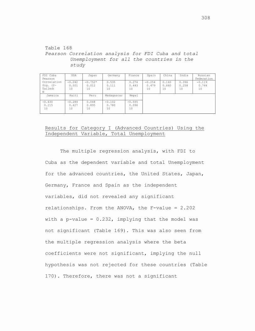
308

Table 168 Pearson Correlation analysis for FDI Cuba and total

Unemployment for all the countries in the study

FDI Cuba Pearson Correlation Sig. (2-Tailed) N

USA Japan Germany France Spain China India Russian Federation

-0.242 0.501 10

-0.752* 0.012 10

0.535 0.111 10

0.274 0.443 10

-0.254 0.479 10

0.160 0.660 10

0.396 0.258 10

-0.119 0.744 10

Jamaica Haiti Peru Madagascar Nepal

-0.430 0.215 10

-0.284 0.427 10

0.048 0.895 10

-0.102 0.780 10

-0.555 0.096 10

Results for Category I (Advanced Countries) Using the Independent Variable, Total Unemployment

The multiple regression analysis, with FDI to

Cuba as the dependent variable and total Unemployment

for the advanced countries, the United States, Japan,

Germany, France and Spain as the independent

variables, did not revealed any significant

relationships. From the ANOVA, the F-value = 2.202

with a p-value = 0.232, implying that the model was

not significant (Table 169). This was also seen from

the multiple regression analysis where the beta

coefficients were not significant, implying the null

hypothesis was not rejected for these countries (Table

170). Therefore, there was not a significant

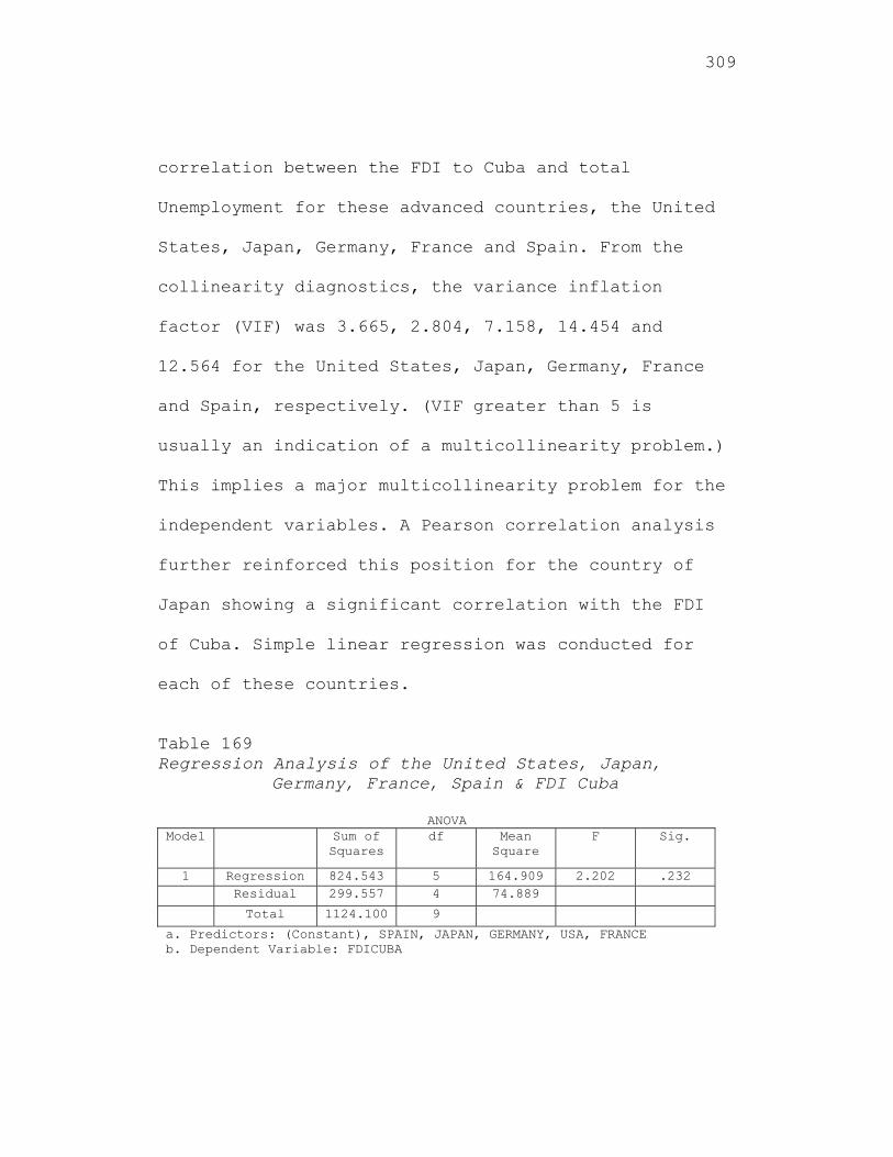
309

correlation between the FDI to Cuba and total

Unemployment for these advanced countries, the United

States, Japan, Germany, France and Spain. From the

collinearity diagnostics, the variance inflation

factor (VIF) was 3.665, 2.804, 7.158, 14.454 and

12.564 for the United States, Japan, Germany, France

and Spain, respectively. (VIF greater than 5 is

usually an indication of a multicollinearity problem.)

This implies a major multicollinearity problem for the

independent variables. A Pearson correlation analysis

further reinforced this position for the country of

Japan showing a significant correlation with the FDI

of Cuba. Simple linear regression was conducted for

each of these countries.

Table 169 Regression Analysis of the United States, Japan,

Germany, France, Spain & FDI Cuba

ANOVA Model Sum of

Squares df Mean

Square F Sig.

1 Regression 824.543 5 164.909 2.202 .232 Residual 299.557 4 74.889

Total 1124.100 9

a. Predictors: (Constant), SPAIN, JAPAN, GERMANY, USA, FRANCE b. Dependent Variable: FDICUBA

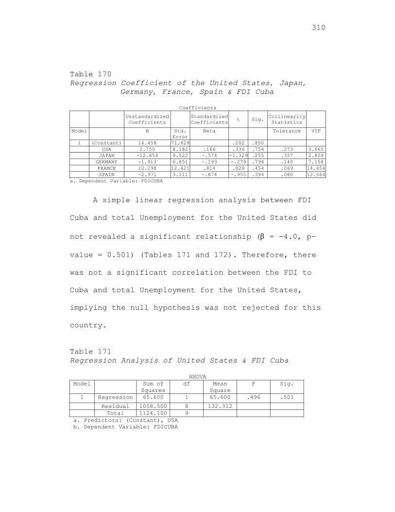
310

Table 170 Regression Coefficient of the United States, Japan,

Germany, France, Spain & FDI Cuba

Coefficients Unstandardized

Coefficients Standardized

Coefficientst Sig. Collinearity

Statistics

Model B Std. Error

Beta Tolerance VIF

1 (Constant) 14.458 71.629 .202 .850 USA 2.750 8.182 .166 .336 .754 .273 3.665 JAPAN -12.654 9.522 -.574 -1.329 .255 .357 2.804 GERMANY -1.913 6.851 -.193 -.279 .794 .140 7.158 FRANCE 10.298 12.421 .814 .829 .454 .069 14.454 SPAIN -2.971 3.111 -.874 -.955 .394 .080 12.564

a. Dependent Variable: FDICUBA

A simple linear regression analysis between FDI

Cuba and total Unemployment for the United States did

not revealed a significant relationship ( = -4.0, p-

value = 0.501) (Tables 171 and 172). Therefore, there

was not a significant correlation between the FDI to

Cuba and total Unemployment for the United States,

implying the null hypothesis was not rejected for this

country.

Table 171 Regression Analysis of United States & FDI Cuba

ANOVA Model Sum of

Squares df Mean

Square F Sig.

1 Regression 65.600 1 65.600 .496 .501

Residual 1058.500 8 132.312 Total 1124.100 9

a. Predictors: (Constant), USA b. Dependent Variable: FDICUBA

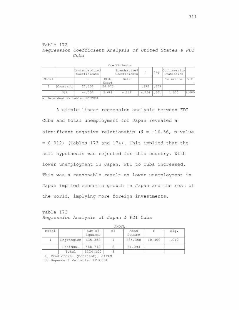
311

Table 172 Regression Coefficient Analysis of United States & FDI

Cuba

Coefficients Unstandardized

Coefficients Standardized Coefficients t Sig.

Collinearity Statistics

Model B Std. Error

Beta Tolerance VIF

1 (Constant) 27.300 28.073 .972 .359

USA -4.000 5.681 -.242 -.704 .501 1.000 1.000

a. Dependent Variable: FDICUBA

A simple linear regression analysis between FDI

Cuba and total unemployment for Japan revealed a

significant negative relationship ( = -16.56, p-value

= 0.012) (Tables 173 and 174). This implied that the

null hypothesis was rejected for this country. With

lower unemployment in Japan, FDI to Cuba increased.

This was a reasonable result as lower unemployment in

Japan implied economic growth in Japan and the rest of

the world, implying more foreign investments.

Table 173 Regression Analysis of Japan & FDI Cuba

ANOVA

Model Sum of Squares

df Mean Square

F Sig.

1 Regression 635.358 1 635.358 10.400 .012

Residual 488.742 8 61.093 Total 1124.100 9

a. Predictors: (Constant), JAPAN b. Dependent Variable: FDICUBA

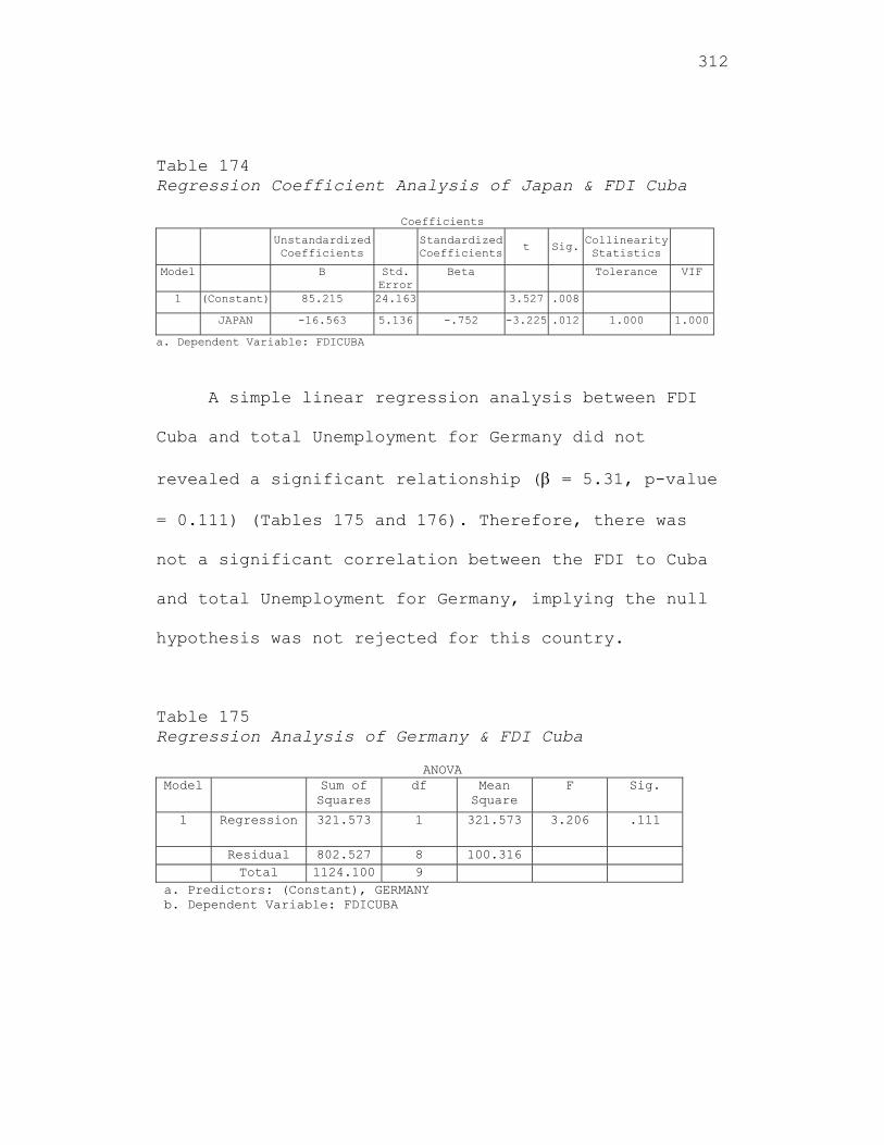
312

Table 174 Regression Coefficient Analysis of Japan & FDI Cuba

Coefficients

Unstandardized Coefficients

Standardized Coefficients t Sig.

Collinearity Statistics

Model B Std. Error

Beta Tolerance VIF

1 (Constant) 85.215 24.163 3.527 .008

JAPAN -16.563 5.136 -.752 -3.225 .012 1.000 1.000

a. Dependent Variable: FDICUBA

A simple linear regression analysis between FDI

Cuba and total Unemployment for Germany did not

revealed a significant relationship ( = 5.31, p-value

= 0.111) (Tables 175 and 176). Therefore, there was

not a significant correlation between the FDI to Cuba

and total Unemployment for Germany, implying the null

hypothesis was not rejected for this country.

Table 175 Regression Analysis of Germany & FDI Cuba

ANOVA

Model Sum of Squares

df Mean Square

F Sig.

1 Regression 321.573 1 321.573 3.206 .111

Residual 802.527 8 100.316 Total 1124.100 9

a. Predictors: (Constant), GERMANY b. Dependent Variable: FDICUBA

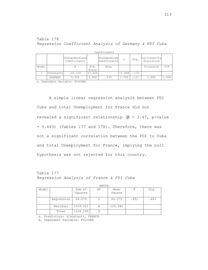
313

Table 176 Regression Coefficient Analysis of Germany & FDI Cuba

Coefficients

Unstandardized Coefficients

Standardized Coefficients

t Sig. Collinearity Statistics

Model B Std. Error

Beta Tolerance VIF

1 (Constant) -41.120 27.450 -1.498 .173

GERMANY 5.306 2.964 .535 1.790 .111 1.000 1.000

a. Dependent Variable: FDICUBA

A simple linear regression analysis between FDI

Cuba and total Unemployment for France did not

revealed a significant relationship ( = 3.47, p-value

= 0.443) (Tables 177 and 178). Therefore, there was

not a significant correlation between the FDI to Cuba

and total Unemployment for France, implying the null

hypothesis was not rejected for this country.

Table 177 Regression Analysis of France & FDI Cuba

ANOVA

Model Sum of Squares

df Mean Square

F Sig.

Regression 84.579 1 84.579 .651 .443

Residual 1039.521 8 129.940

Total 1124.100 9

a. Predictors: (Constant), FRANCE b. Dependent Variable: FDICUBA

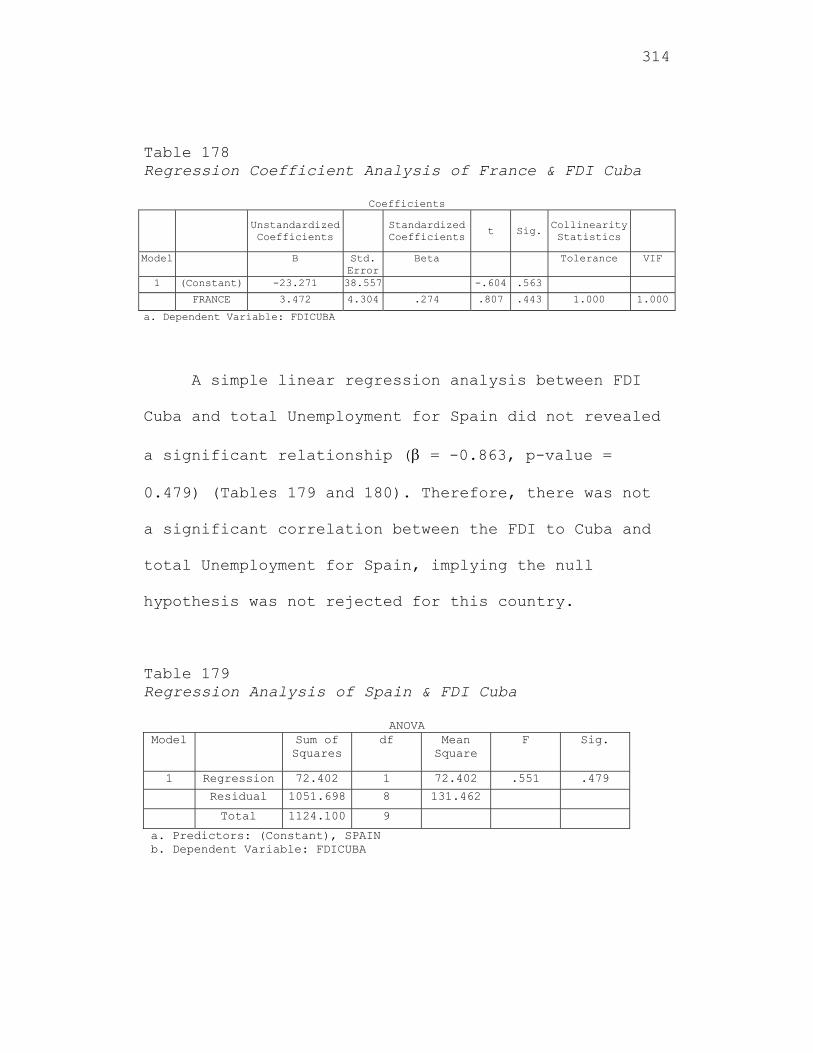
314

Table 178 Regression Coefficient Analysis of France & FDI Cuba

Coefficients

Unstandardized Coefficients

Standardized Coefficients t Sig.

Collinearity Statistics

Model B Std. Error

Beta Tolerance VIF

1 (Constant) -23.271 38.557 -.604 .563

FRANCE 3.472 4.304 .274 .807 .443 1.000 1.000

a. Dependent Variable: FDICUBA

A simple linear regression analysis between FDI

Cuba and total Unemployment for Spain did not revealed

a significant relationship ( = -0.863, p-value =

0.479) (Tables 179 and 180). Therefore, there was not

a significant correlation between the FDI to Cuba and

total Unemployment for Spain, implying the null

hypothesis was not rejected for this country.

Table 179 Regression Analysis of Spain & FDI Cuba

ANOVA Model Sum of

Squares df Mean

Square F Sig.

1 Regression 72.402 1 72.402 .551 .479

Residual 1051.698 8 131.462

Total 1124.100 9

a. Predictors: (Constant), SPAIN b. Dependent Variable: FDICUBA

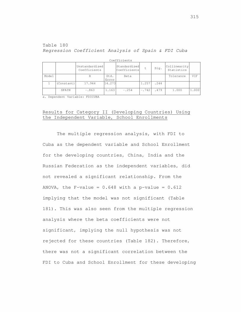
315

Table 180 Regression Coefficient Analysis of Spain & FDI Cuba

Coefficients

Unstandardized Coefficients

Standardized Coefficients t Sig.

Collinearity Statistics

Model B Std. Error

Beta Tolerance VIF

1 (Constant) 17.944 14.273 1.257 .244

SPAIN -.863 1.163 -.254 -.742 .479 1.000 1.000

a. Dependent Variable: FDICUBA

Results for Category II (Developing Countries) Using the Independent Variable, School Enrollments

The multiple regression analysis, with FDI to

Cuba as the dependent variable and School Enrollment

for the developing countries, China, India and the

Russian Federation as the independent variables, did

not revealed a significant relationship. From the

ANOVA, the F-value = 0.648 with a p-value = 0.612

implying that the model was not significant (Table

181). This was also seen from the multiple regression

analysis where the beta coefficients were not

significant, implying the null hypothesis was not

rejected for these countries (Table 182). Therefore,

there was not a significant correlation between the

FDI to Cuba and School Enrollment for these developing

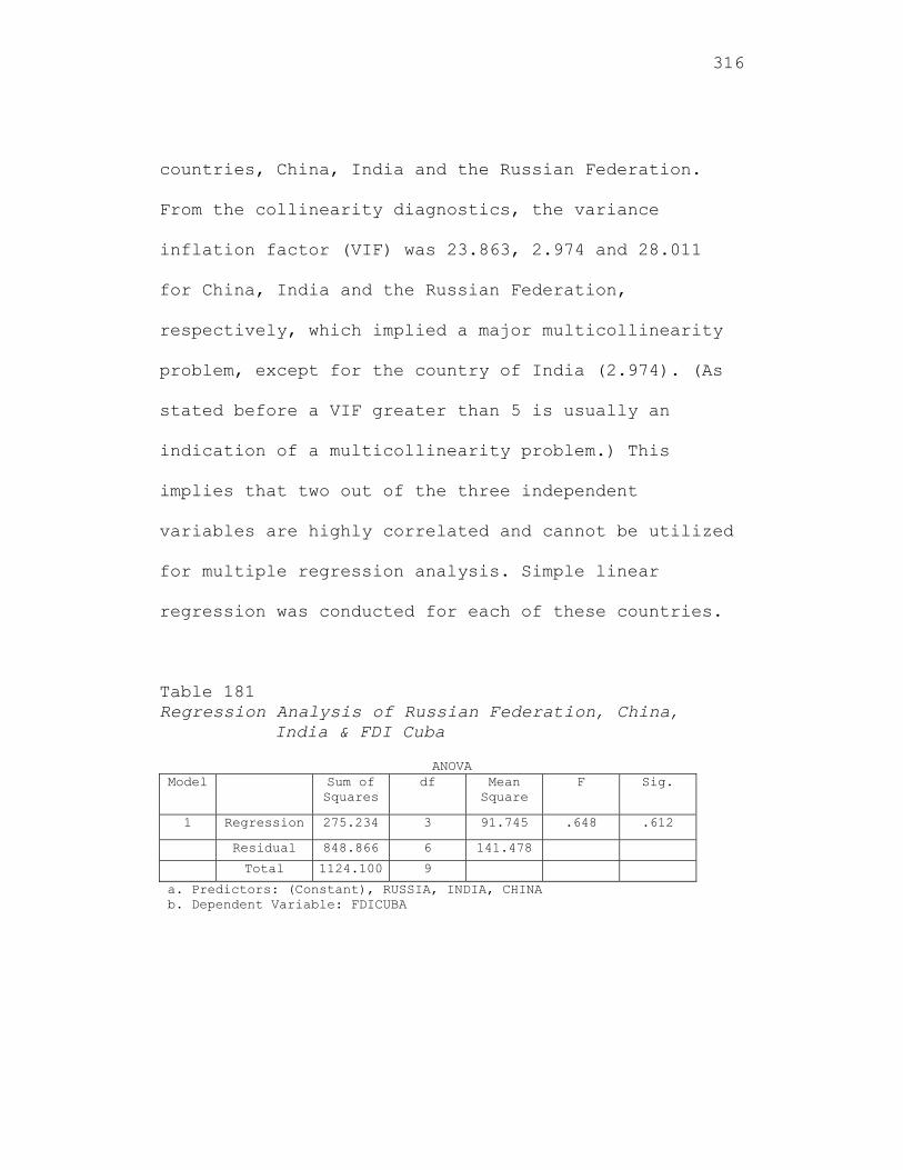
316

countries, China, India and the Russian Federation.

From the collinearity diagnostics, the variance

inflation factor (VIF) was 23.863, 2.974 and 28.011

for China, India and the Russian Federation,

respectively, which implied a major multicollinearity

problem, except for the country of India (2.974). (As

stated before a VIF greater than 5 is usually an

indication of a multicollinearity problem.) This

implies that two out of the three independent

variables are highly correlated and cannot be utilized

for multiple regression analysis. Simple linear

regression was conducted for each of these countries.

Table 181 Regression Analysis of Russian Federation, China,

India & FDI Cuba

ANOVA Model Sum of

Squares df Mean

Square F Sig.

1 Regression 275.234 3 91.745 .648 .612

Residual 848.866 6 141.478

Total 1124.100 9

a. Predictors: (Constant), RUSSIA, INDIA, CHINA b. Dependent Variable: FDICUBA

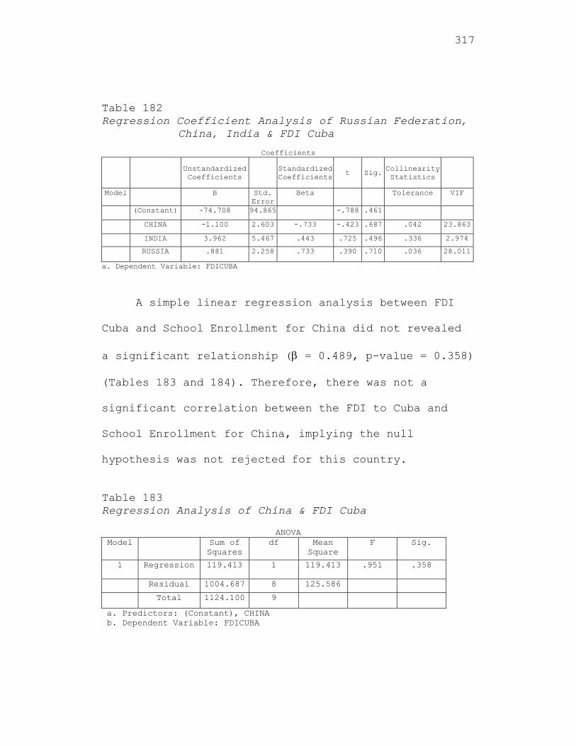
317

Table 182 Regression Coefficient Analysis of Russian Federation,

China, India & FDI Cuba

Coefficients

Unstandardized Coefficients

Standardized Coefficients

t Sig. Collinearity Statistics

Model B Std. Error

Beta Tolerance VIF

(Constant) -74.708 94.865 -.788 .461

CHINA -1.100 2.603 -.733 -.423 .687 .042 23.863

INDIA 3.962 5.467 .443 .725 .496 .336 2.974

RUSSIA .881 2.258 .733 .390 .710 .036 28.011

a. Dependent Variable: FDICUBA

A simple linear regression analysis between FDI

Cuba and School Enrollment for China did not revealed

a significant relationship ( = 0.489, p-value = 0.358)

(Tables 183 and 184). Therefore, there was not a

significant correlation between the FDI to Cuba and

School Enrollment for China, implying the null

hypothesis was not rejected for this country.

Table 183 Regression Analysis of China & FDI Cuba

ANOVA Model Sum of

Squares df Mean

Square F Sig.

1 Regression 119.413 1 119.413 .951 .358

Residual 1004.687 8 125.586

Total 1124.100 9

a. Predictors: (Constant), CHINA b. Dependent Variable: FDICUBA

318

Table 184 Regression Coefficient Analysis of China & FDI Cuba

Coefficients

Unstandardized Coefficients

Standardized Coefficients t Sig.

Collinearity Statistics

Model B Std. Error

Beta Tolerance VIF

1 (Constant) 1.097 7.643 .144 .889

CHINA .489 .502 .326 .975 .358 1.000 1.000

a. Dependent Variable: FDICUBA

A simple linear regression analysis between FDI

Cuba and School Enrollment for India did not revealed

a significant relationship ( = 4.21, p-value = 0.169)

(Tables 185 and 186). Therefore, there was not a

significant correlation between the FDI to Cuba and

School Enrollment for India, implying the null

hypothesis was not rejected for this country.

Table 185 Regression Analysis of India & FDI Cuba

ANOVA Model Sum of

Squares df Mean

Square F Sig.

1 Regression 249.817 1 249.817 2.286 .169

Residual 874.283 8 109.285

Total 1124.100 9

a. Predictors: (Constant), INDIA b. Dependent Variable: FDICUBA

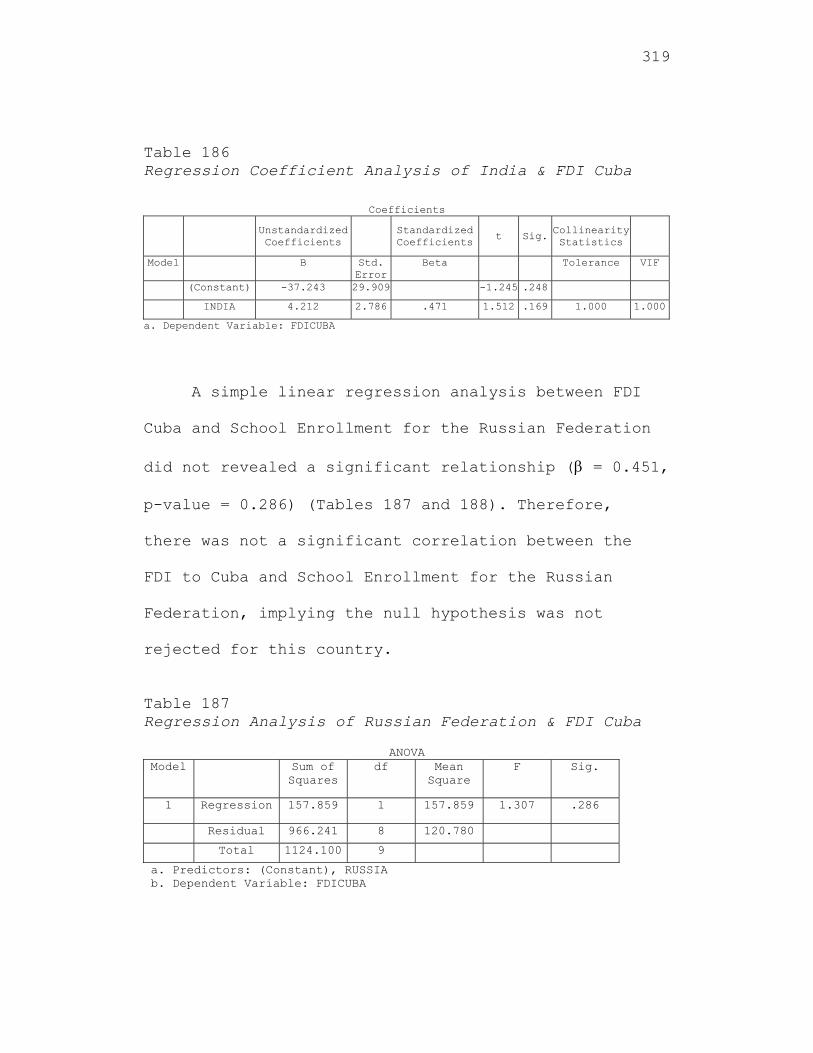
319

Table 186 Regression Coefficient Analysis of India & FDI Cuba

Coefficients

Unstandardized Coefficients

Standardized Coefficients

t Sig. Collinearity Statistics

Model B Std. Error

Beta Tolerance VIF

(Constant) -37.243 29.909 -1.245 .248

INDIA 4.212 2.786 .471 1.512 .169 1.000 1.000

a. Dependent Variable: FDICUBA

A simple linear regression analysis between FDI

Cuba and School Enrollment for the Russian Federation

did not revealed a significant relationship ( = 0.451,

p-value = 0.286) (Tables 187 and 188). Therefore,

there was not a significant correlation between the

FDI to Cuba and School Enrollment for the Russian

Federation, implying the null hypothesis was not

rejected for this country.

Table 187 Regression Analysis of Russian Federation & FDI Cuba

ANOVA Model Sum of

Squares df Mean

Square F Sig.

1 Regression 157.859 1 157.859 1.307 .286

Residual 966.241 8 120.780

Total 1124.100 9

a. Predictors: (Constant), RUSSIA b. Dependent Variable: FDICUBA

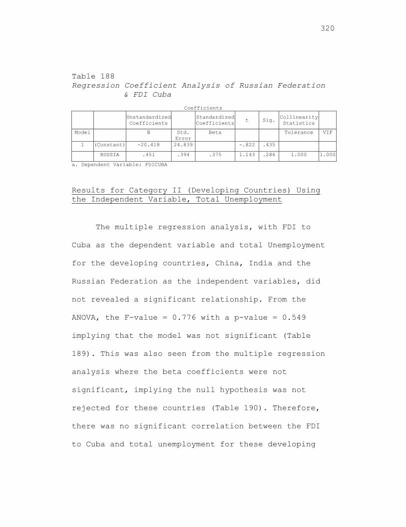
320

Table 188 Regression Coefficient Analysis of Russian Federation

& FDI Cuba

Coefficients Unstandardized

Coefficients Standardized

Coefficientst Sig. Collinearity

Statistics

Model B Std. Error

Beta Tolerance VIF

1 (Constant) -20.418 24.839 -.822 .435

RUSSIA .451 .394 .375 1.143 .286 1.000 1.000

a. Dependent Variable: FDICUBA

Results for Category II (Developing Countries) Using the Independent Variable, Total Unemployment

The multiple regression analysis, with FDI to

Cuba as the dependent variable and total Unemployment

for the developing countries, China, India and the

Russian Federation as the independent variables, did

not revealed a significant relationship. From the

ANOVA, the F-value = 0.776 with a p-value = 0.549

implying that the model was not significant (Table

189). This was also seen from the multiple regression

analysis where the beta coefficients were not

significant, implying the null hypothesis was not

rejected for these countries (Table 190). Therefore,

there was no significant correlation between the FDI

to Cuba and total unemployment for these developing

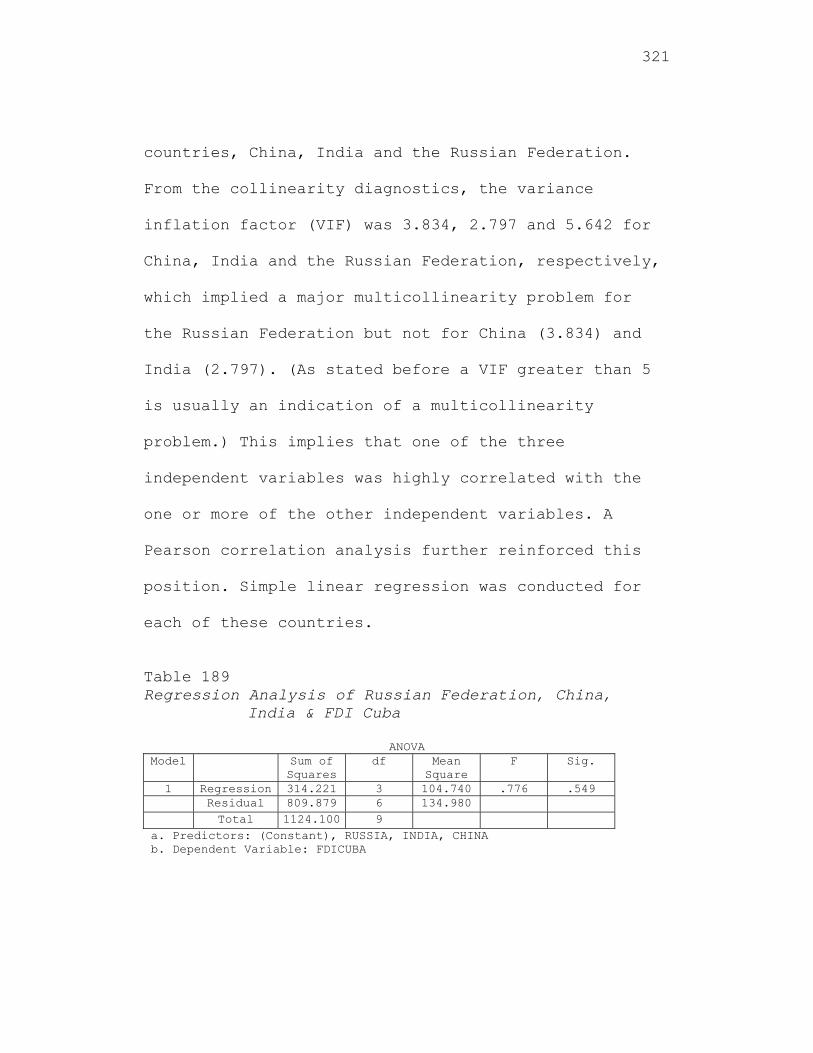
321

countries, China, India and the Russian Federation.

From the collinearity diagnostics, the variance

inflation factor (VIF) was 3.834, 2.797 and 5.642 for

China, India and the Russian Federation, respectively,

which implied a major multicollinearity problem for

the Russian Federation but not for China (3.834) and

India (2.797). (As stated before a VIF greater than 5

is usually an indication of a multicollinearity

problem.) This implies that one of the three

independent variables was highly correlated with the

one or more of the other independent variables. A

Pearson correlation analysis further reinforced this

position. Simple linear regression was conducted for

each of these countries.

Table 189 Regression Analysis of Russian Federation, China,

India & FDI Cuba

ANOVA Model Sum of

Squares df Mean

Square F Sig.

1 Regression 314.221 3 104.740 .776 .549 Residual 809.879 6 134.980 Total 1124.100 9

a. Predictors: (Constant), RUSSIA, INDIA, CHINA b. Dependent Variable: FDICUBA

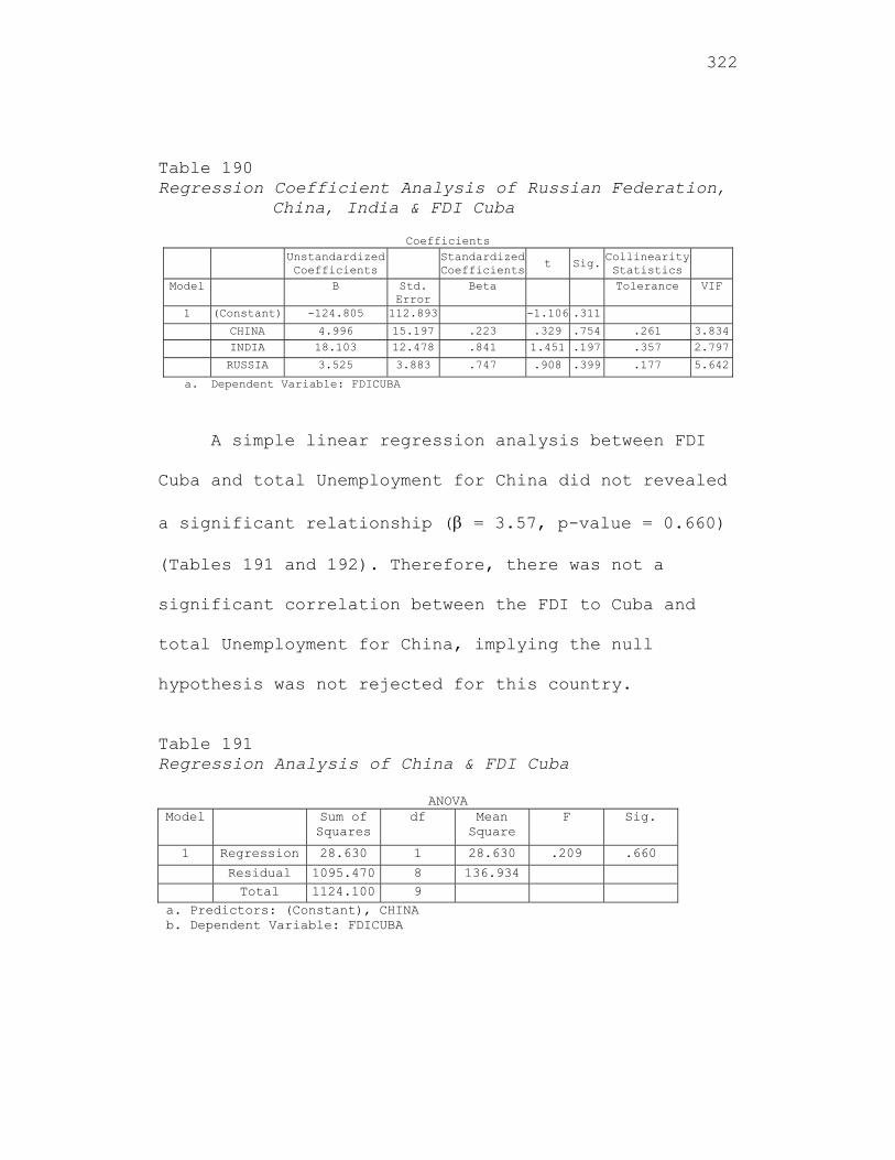
322

Table 190 Regression Coefficient Analysis of Russian Federation,

China, India & FDI Cuba

Coefficients Unstandardized

Coefficients

Standardized Coefficients

t Sig.Collinearity Statistics

Model B Std. Error

Beta Tolerance VIF

1 (Constant) -124.805 112.893 -1.106 .311

CHINA 4.996 15.197 .223 .329 .754 .261 3.834 INDIA 18.103 12.478 .841 1.451 .197 .357 2.797

RUSSIA 3.525 3.883 .747 .908 .399 .177 5.642

a. Dependent Variable: FDICUBA

A simple linear regression analysis between FDI

Cuba and total Unemployment for China did not revealed

a significant relationship ( = 3.57, p-value = 0.660)

(Tables 191 and 192). Therefore, there was not a

significant correlation between the FDI to Cuba and

total Unemployment for China, implying the null

hypothesis was not rejected for this country.

Table 191 Regression Analysis of China & FDI Cuba

ANOVA Model Sum of

Squares df Mean

Square F Sig.

1 Regression 28.630 1 28.630 .209 .660

Residual 1095.470 8 136.934 Total 1124.100 9

a. Predictors: (Constant), CHINA b. Dependent Variable: FDICUBA

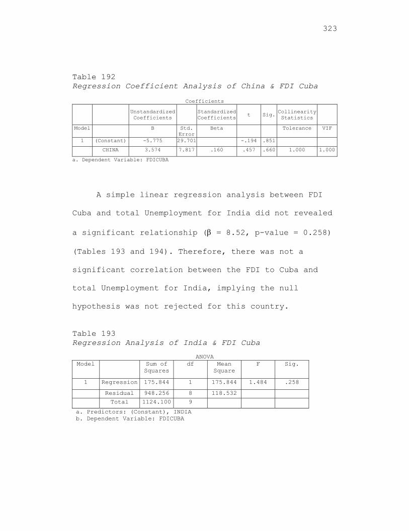
323

Table 192 Regression Coefficient Analysis of China & FDI Cuba

Coefficients

Unstandardized Coefficients

Standardized Coefficients t Sig.

Collinearity Statistics

Model B Std. Error

Beta Tolerance VIF

1 (Constant) -5.775 29.701 -.194 .851

CHINA 3.574 7.817 .160 .457 .660 1.000 1.000

a. Dependent Variable: FDICUBA

A simple linear regression analysis between FDI

Cuba and total Unemployment for India did not revealed

a significant relationship ( = 8.52, p-value = 0.258)

(Tables 193 and 194). Therefore, there was not a

significant correlation between the FDI to Cuba and

total Unemployment for India, implying the null

hypothesis was not rejected for this country.

Table 193 Regression Analysis of India & FDI Cuba

ANOVA Model Sum of

Squares df Mean

Square F Sig.

1 Regression 175.844 1 175.844 1.484 .258

Residual 948.256 8 118.532

Total 1124.100 9

a. Predictors: (Constant), INDIA b. Dependent Variable: FDICUBA

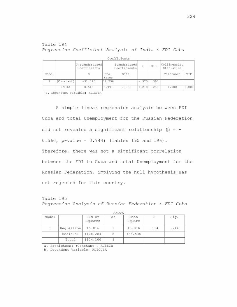
324

Table 194 Regression Coefficient Analysis of India & FDI Cuba

Coefficients

Unstandardized Coefficients

Standardized Coefficients t Sig.

Collinearity Statistics

Model B Std. Error

Beta Tolerance VIF

1 (Constant) -31.045 31.996 -.970 .360

INDIA 8.515 6.991 .396 1.218 .258 1.000 1.000

a. Dependent Variable: FDICUBA

A simple linear regression analysis between FDI

Cuba and total Unemployment for the Russian Federation

did not revealed a significant relationship ( = -

0.560, p-value = 0.744) (Tables 195 and 196).

Therefore, there was not a significant correlation

between the FDI to Cuba and total Unemployment for the

Russian Federation, implying the null hypothesis was

not rejected for this country.

Table 195 Regression Analysis of Russian Federation & FDI Cuba

ANOVA Model Sum of

Squares df Mean

Square F Sig.

1 Regression 15.816 1 15.816 .114 .744

Residual 1108.284 8 138.536

Total 1124.100 9

a. Predictors: (Constant), RUSSIA b. Dependent Variable: FDICUBA

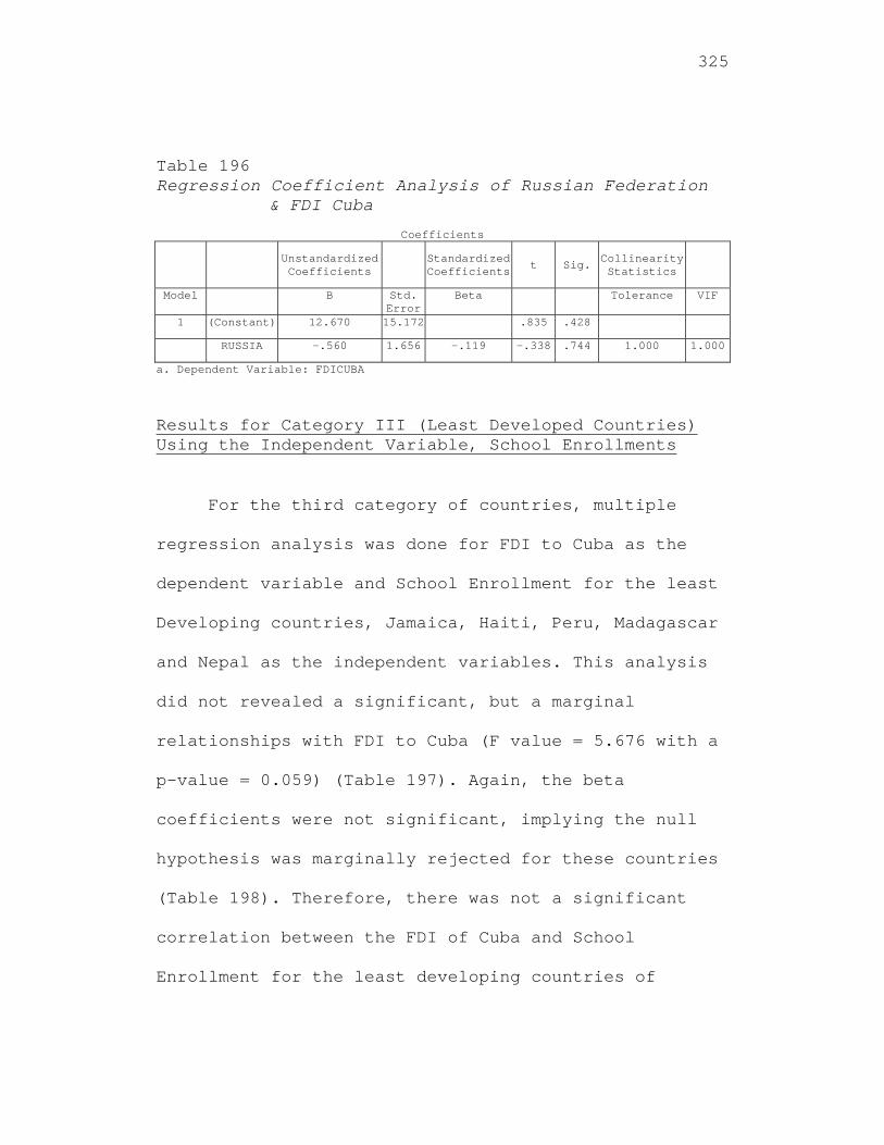
325

Table 196 Regression Coefficient Analysis of Russian Federation

& FDI Cuba

Coefficients

Unstandardized Coefficients

Standardized Coefficients

t Sig. Collinearity Statistics

Model B Std. Error

Beta Tolerance VIF

1 (Constant) 12.670 15.172 .835 .428

RUSSIA -.560 1.656 -.119 -.338 .744 1.000 1.000

a. Dependent Variable: FDICUBA Results for Category III (Least Developed Countries) Using the Independent Variable, School Enrollments

For the third category of countries, multiple

regression analysis was done for FDI to Cuba as the

dependent variable and School Enrollment for the least

Developing countries, Jamaica, Haiti, Peru, Madagascar

and Nepal as the independent variables. This analysis

did not revealed a significant, but a marginal

relationships with FDI to Cuba (F value = 5.676 with a

p-value = 0.059) (Table 197). Again, the beta

coefficients were not significant, implying the null

hypothesis was marginally rejected for these countries

(Table 198). Therefore, there was not a significant

correlation between the FDI of Cuba and School

Enrollment for the least developing countries of

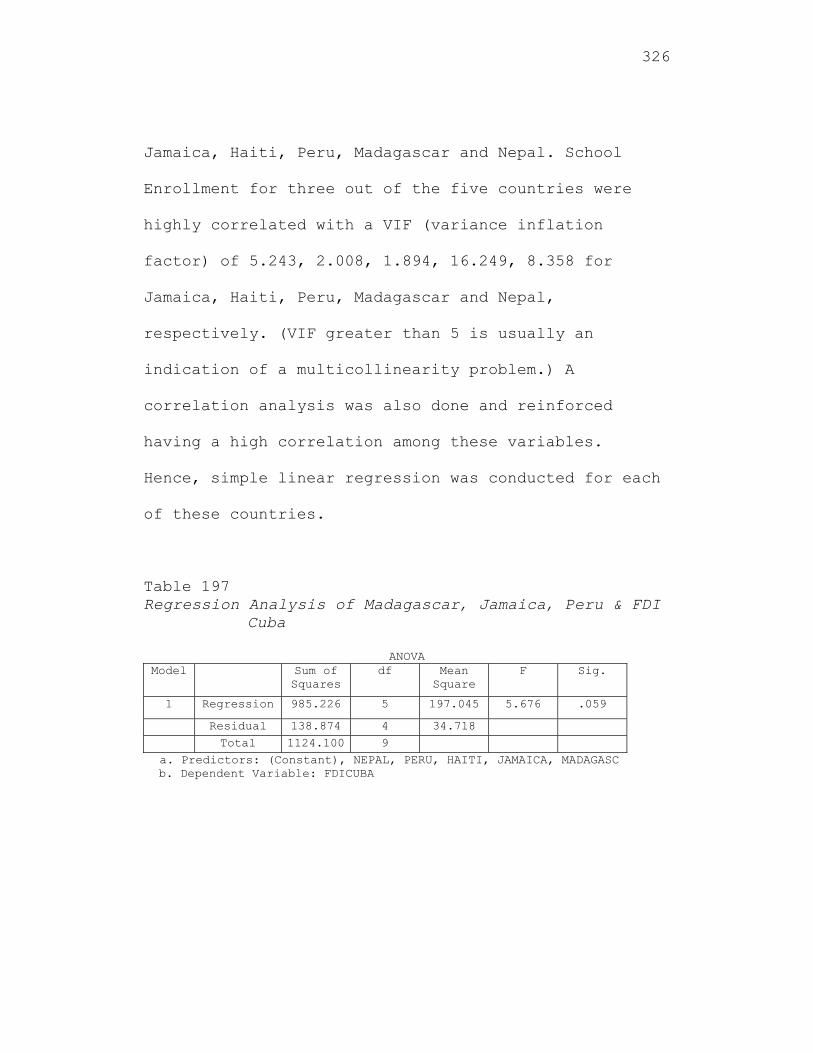
326

Jamaica, Haiti, Peru, Madagascar and Nepal. School

Enrollment for three out of the five countries were

highly correlated with a VIF (variance inflation

factor) of 5.243, 2.008, 1.894, 16.249, 8.358 for

Jamaica, Haiti, Peru, Madagascar and Nepal,

respectively. (VIF greater than 5 is usually an

indication of a multicollinearity problem.) A

correlation analysis was also done and reinforced

having a high correlation among these variables.

Hence, simple linear regression was conducted for each

of these countries.

Table 197 Regression Analysis of Madagascar, Jamaica, Peru & FDI

Cuba

ANOVA Model Sum of

Squares df Mean

Square F Sig.

1 Regression 985.226 5 197.045 5.676 .059

Residual 138.874 4 34.718

Total 1124.100 9 a. Predictors: (Constant), NEPAL, PERU, HAITI, JAMAICA, MADAGASC

b. Dependent Variable: FDICUBA

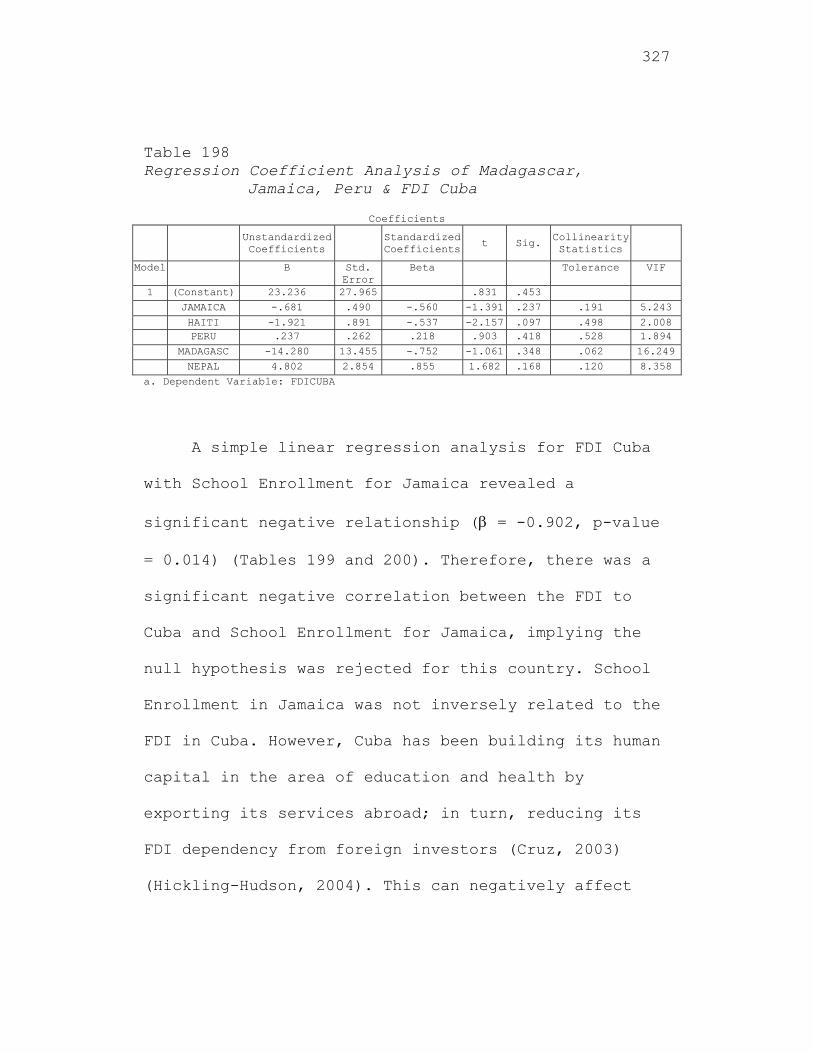
327

Table 198 Regression Coefficient Analysis of Madagascar,

Jamaica, Peru & FDI Cuba

Coefficients Unstandardized

Coefficients Standardized

Coefficientst Sig. Collinearity

Statistics

Model B Std. Error

Beta Tolerance VIF

1 (Constant) 23.236 27.965 .831 .453

JAMAICA -.681 .490 -.560 -1.391 .237 .191 5.243

HAITI -1.921 .891 -.537 -2.157 .097 .498 2.008 PERU .237 .262 .218 .903 .418 .528 1.894

MADAGASC -14.280 13.455 -.752 -1.061 .348 .062 16.249

NEPAL 4.802 2.854 .855 1.682 .168 .120 8.358

a. Dependent Variable: FDICUBA

A simple linear regression analysis for FDI Cuba

with School Enrollment for Jamaica revealed a

significant negative relationship ( = -0.902, p-value

= 0.014) (Tables 199 and 200). Therefore, there was a

significant negative correlation between the FDI to

Cuba and School Enrollment for Jamaica, implying the

null hypothesis was rejected for this country. School

Enrollment in Jamaica was not inversely related to the

FDI in Cuba. However, Cuba has been building its human

capital in the area of education and health by

exporting its services abroad; in turn, reducing its

FDI dependency from foreign investors (Cruz, 2003)

(Hickling-Hudson, 2004). This can negatively affect

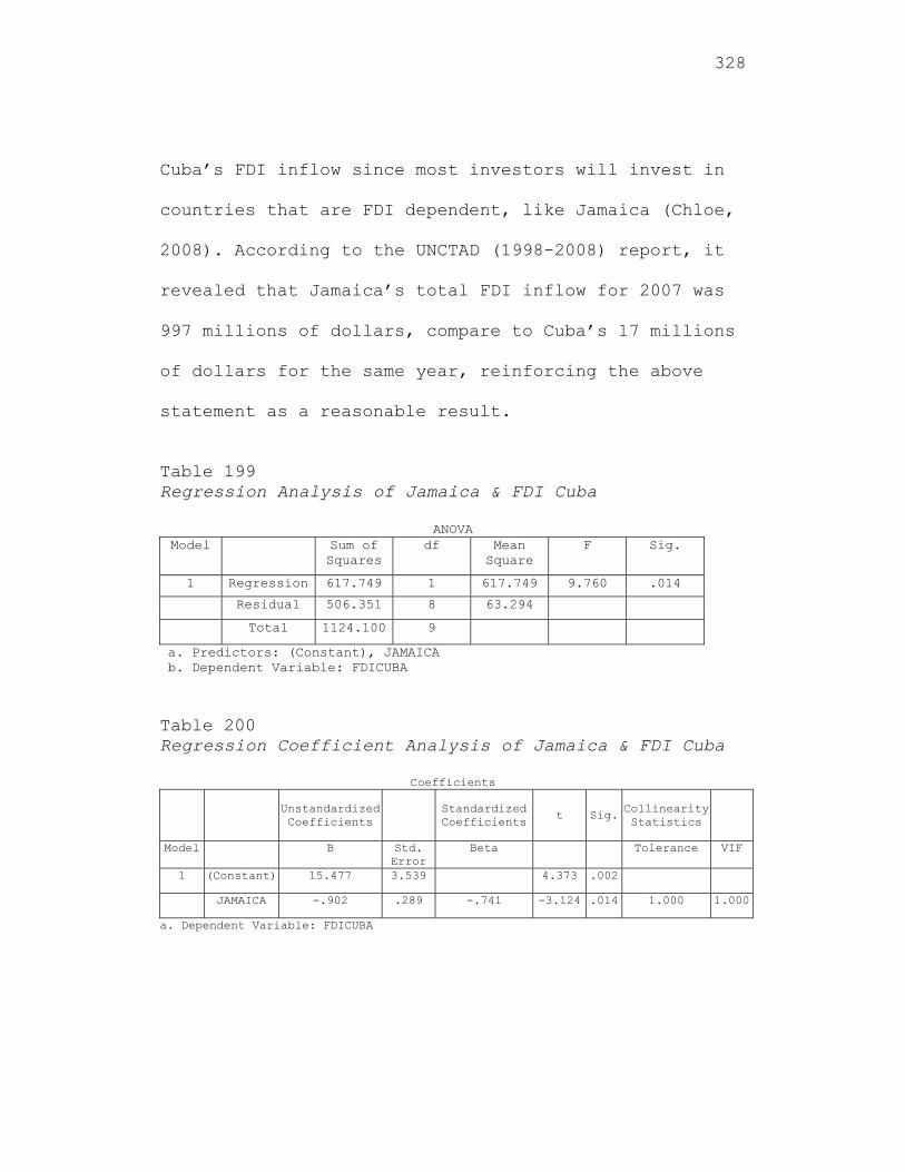
328

Cuba’s FDI inflow since most investors will invest in

countries that are FDI dependent, like Jamaica (Chloe,

2008). According to the UNCTAD (1998-2008) report, it

revealed that Jamaica’s total FDI inflow for 2007 was

997 millions of dollars, compare to Cuba’s 17 millions

of dollars for the same year, reinforcing the above

statement as a reasonable result.

Table 199 Regression Analysis of Jamaica & FDI Cuba

ANOVA Model Sum of

Squares df Mean

Square F Sig.

1 Regression 617.749 1 617.749 9.760 .014

Residual 506.351 8 63.294

Total 1124.100 9

a. Predictors: (Constant), JAMAICA b. Dependent Variable: FDICUBA

Table 200 Regression Coefficient Analysis of Jamaica & FDI Cuba

Coefficients

Unstandardized Coefficients

Standardized Coefficients

t Sig. Collinearity Statistics

Model B Std. Error

Beta Tolerance VIF

1 (Constant) 15.477 3.539 4.373 .002

JAMAICA -.902 .289 -.741 -3.124 .014 1.000 1.000

a. Dependent Variable: FDICUBA

329

A simple linear regression analysis between FDI

Cuba and School Enrollment for Haiti revealed a

significant negative relationship ( = -2.60, p-value =

0.017) (Tables 201 and 202). Therefore, there was a

significant negative relationship between the FDI to

Cuba and School Enrollment for Haiti, implying the

null hypothesis was rejected for this country. In

2008, the Cuban government main source of income was

exporting its human capital services, like education

to less developed countries with a lower education

standard, like Haiti (Chloe, 2008). However, such

services to Haiti can reduce Cuba’s FDI inflow since

Cuba’s less dependency would redirect countries to

invest elsewhere. According to the UNCTAD (1998-2008)

report, it revealed that Haiti’s total FDI inflow for

2007 was 75 millions of dollars, compare to Cuba’s 17

millions of dollars for the same year, reinforcing the

above statement as a reasonable result.

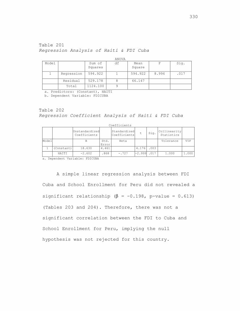
330

Table 201 Regression Analysis of Haiti & FDI Cuba

ANOVA Model Sum of

Squares df Mean

Square F Sig.

1 Regression 594.922 1 594.922 8.994 .017

Residual 529.178 8 66.147

Total 1124.100 9

a. Predictors: (Constant), HAITI b. Dependent Variable: FDICUBA

Table 202 Regression Coefficient Analysis of Haiti & FDI Cuba

Coefficients

Unstandardized Coefficients

Standardized Coefficients t Sig.

Collinearity Statistics

Model B Std. Error

Beta Tolerance VIF

1 (Constant) 18.630 4.461 4.176 .003

HAITI -2.602 .868 -.727 -2.999 .017 1.000 1.000

a. Dependent Variable: FDICUBA

A simple linear regression analysis between FDI

Cuba and School Enrollment for Peru did not revealed a

significant relationship ( = -0.198, p-value = 0.613)

(Tables 203 and 204). Therefore, there was not a

significant correlation between the FDI to Cuba and

School Enrollment for Peru, implying the null

hypothesis was not rejected for this country.

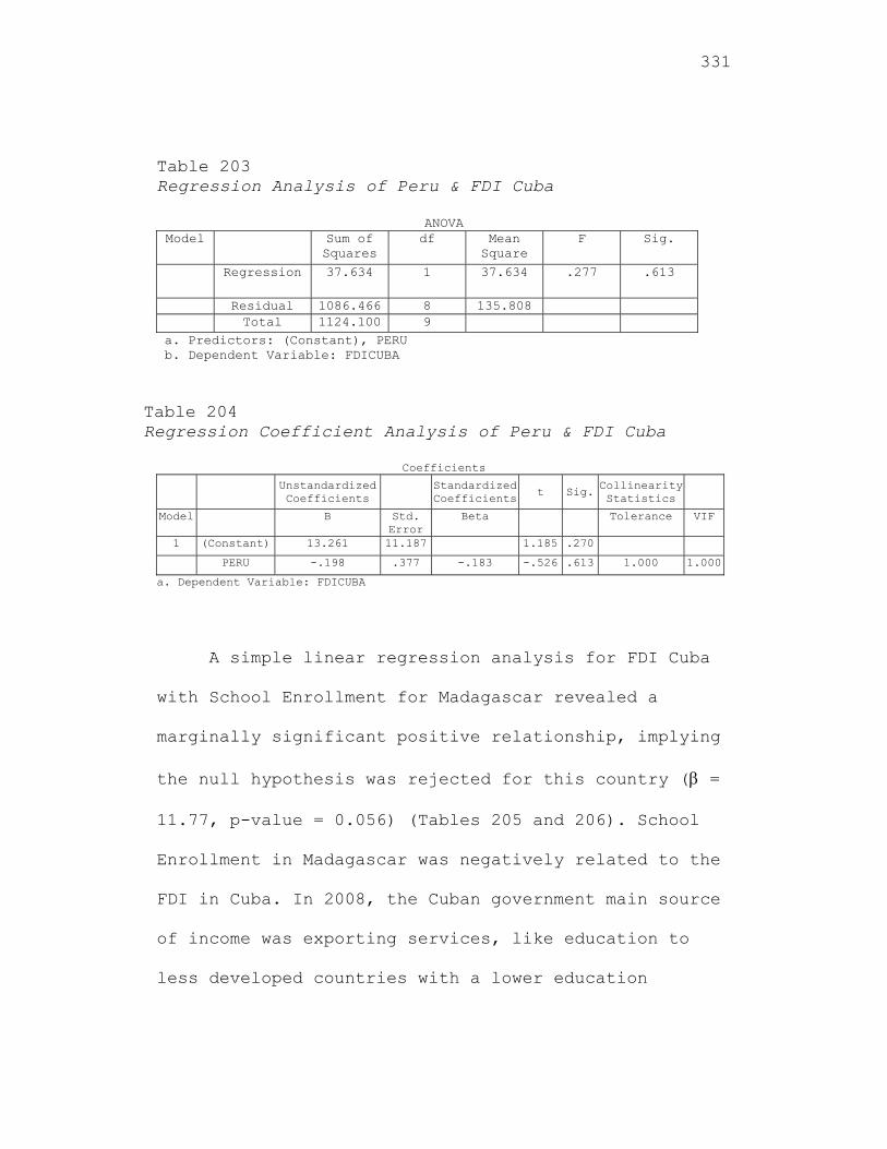
331

Table 203 Regression Analysis of Peru & FDI Cuba

ANOVA Model Sum of

Squares df Mean

Square F Sig.

Regression 37.634 1 37.634 .277 .613

Residual 1086.466 8 135.808 Total 1124.100 9

a. Predictors: (Constant), PERU b. Dependent Variable: FDICUBA

Table 204 Regression Coefficient Analysis of Peru & FDI Cuba

Coefficients Unstandardized

Coefficients Standardized

Coefficientst Sig. Collinearity

Statistics

Model B Std. Error

Beta Tolerance VIF

1 (Constant) 13.261 11.187 1.185 .270

PERU -.198 .377 -.183 -.526 .613 1.000 1.000

a. Dependent Variable: FDICUBA

A simple linear regression analysis for FDI Cuba

with School Enrollment for Madagascar revealed a

marginally significant positive relationship, implying

the null hypothesis was rejected for this country ( =

11.77, p-value = 0.056) (Tables 205 and 206). School

Enrollment in Madagascar was negatively related to the

FDI in Cuba. In 2008, the Cuban government main source

of income was exporting services, like education to

less developed countries with a lower education

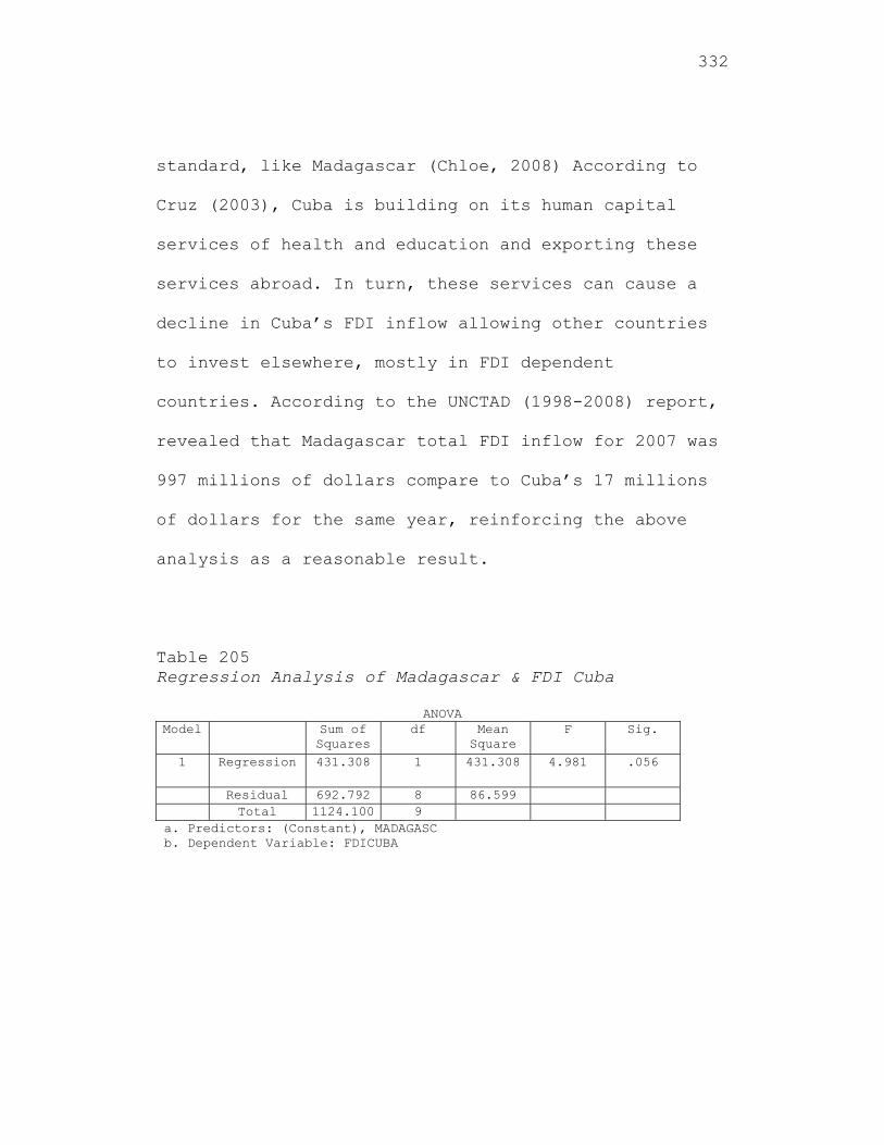
332

standard, like Madagascar (Chloe, 2008) According to

Cruz (2003), Cuba is building on its human capital

services of health and education and exporting these

services abroad. In turn, these services can cause a

decline in Cuba’s FDI inflow allowing other countries

to invest elsewhere, mostly in FDI dependent

countries. According to the UNCTAD (1998-2008) report,

revealed that Madagascar total FDI inflow for 2007 was

997 millions of dollars compare to Cuba’s 17 millions

of dollars for the same year, reinforcing the above

analysis as a reasonable result.

Table 205 Regression Analysis of Madagascar & FDI Cuba

ANOVA Model Sum of

Squares df Mean

Square F Sig.

1 Regression 431.308 1 431.308 4.981 .056

Residual 692.792 8 86.599 Total 1124.100 9

a. Predictors: (Constant), MADAGASC b. Dependent Variable: FDICUBA

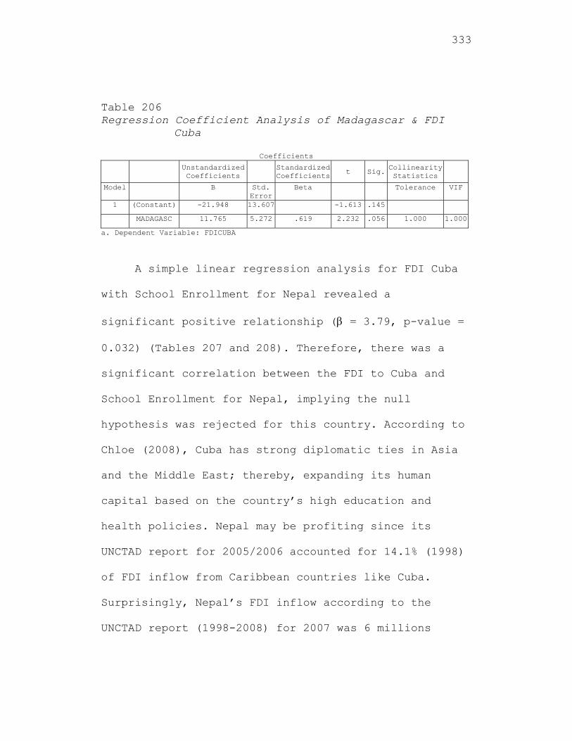
333

Table 206 Regression Coefficient Analysis of Madagascar & FDI

Cuba

Coefficients Unstandardized

Coefficients Standardized Coefficients t Sig.

Collinearity Statistics

Model B Std. Error

Beta Tolerance VIF

1 (Constant) -21.948 13.607 -1.613 .145

MADAGASC 11.765 5.272 .619 2.232 .056 1.000 1.000

a. Dependent Variable: FDICUBA

A simple linear regression analysis for FDI Cuba

with School Enrollment for Nepal revealed a

significant positive relationship ( = 3.79, p-value =

0.032) (Tables 207 and 208). Therefore, there was a

significant correlation between the FDI to Cuba and

School Enrollment for Nepal, implying the null

hypothesis was rejected for this country. According to

Chloe (2008), Cuba has strong diplomatic ties in Asia

and the Middle East; thereby, expanding its human

capital based on the country’s high education and

health policies. Nepal may be profiting since its

UNCTAD report for 2005/2006 accounted for 14.1% (1998)

of FDI inflow from Caribbean countries like Cuba.

Surprisingly, Nepal’s FDI inflow according to the

UNCTAD report (1998-2008) for 2007 was 6 millions

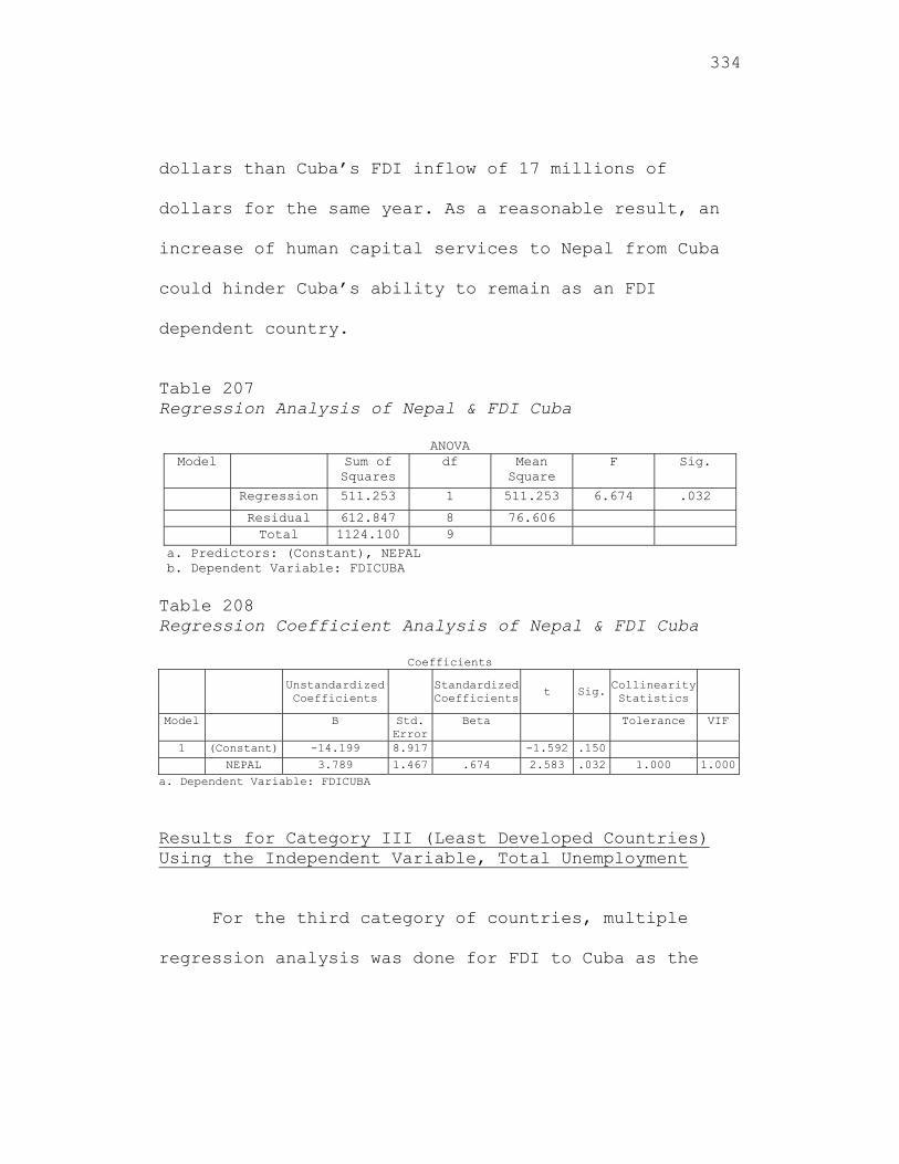
334

dollars than Cuba’s FDI inflow of 17 millions of

dollars for the same year. As a reasonable result, an

increase of human capital services to Nepal from Cuba

could hinder Cuba’s ability to remain as an FDI

dependent country.

Table 207 Regression Analysis of Nepal & FDI Cuba

ANOVA Model Sum of

Squares df Mean

Square F Sig.

Regression 511.253 1 511.253 6.674 .032

Residual 612.847 8 76.606 Total 1124.100 9

a. Predictors: (Constant), NEPAL b. Dependent Variable: FDICUBA

Table 208 Regression Coefficient Analysis of Nepal & FDI Cuba

Coefficients

Unstandardized Coefficients

Standardized Coefficients

t Sig. Collinearity Statistics

Model B Std. Error

Beta Tolerance VIF

1 (Constant) -14.199 8.917 -1.592 .150

NEPAL 3.789 1.467 .674 2.583 .032 1.000 1.000

a. Dependent Variable: FDICUBA

Results for Category III (Least Developed Countries) Using the Independent Variable, Total Unemployment

For the third category of countries, multiple

regression analysis was done for FDI to Cuba as the

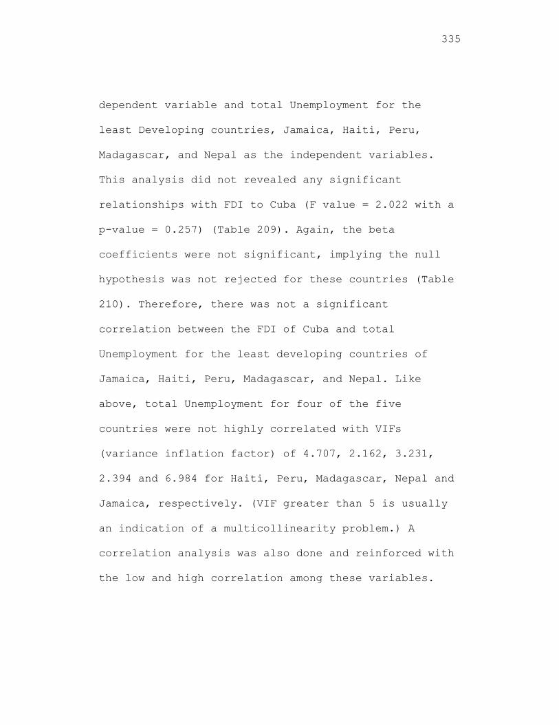
335

dependent variable and total Unemployment for the

least Developing countries, Jamaica, Haiti, Peru,

Madagascar, and Nepal as the independent variables.

This analysis did not revealed any significant

relationships with FDI to Cuba (F value = 2.022 with a

p-value = 0.257) (Table 209). Again, the beta

coefficients were not significant, implying the null

hypothesis was not rejected for these countries (Table

210). Therefore, there was not a significant

correlation between the FDI of Cuba and total

Unemployment for the least developing countries of

Jamaica, Haiti, Peru, Madagascar, and Nepal. Like

above, total Unemployment for four of the five

countries were not highly correlated with VIFs

(variance inflation factor) of 4.707, 2.162, 3.231,

2.394 and 6.984 for Haiti, Peru, Madagascar, Nepal and

Jamaica, respectively. (VIF greater than 5 is usually

an indication of a multicollinearity problem.) A

correlation analysis was also done and reinforced with

the low and high correlation among these variables.

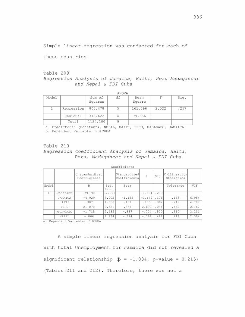
336

Simple linear regression was conducted for each of

these countries.

Table 209 Regression Analysis of Jamaica, Haiti, Peru Madagascar

and Nepal & FDI Cuba

ANOVA Model Sum of

Squares df Mean

Square F Sig.

1 Regression 805.478 5 161.096 2.022 .257

Residual 318.622 4 79.656

Total 1124.100 9

a. Predictors: (Constant), NEPAL, HAITI, PERU, MADAGASC, JAMAICA b. Dependent Variable: FDICUBA Table 210 Regression Coefficient Analysis of Jamaica, Haiti,

Peru, Madagascar and Nepal & FDI Cuba

Coefficients

Unstandardized Coefficients

Standardized Coefficients t Sig.

Collinearity Statistics

Model B Std. Error

Beta Tolerance VIF

1 (Constant) -79.701 57.591 -1.384 .239

JAMAICA -4.929 3.002 -1.155 -1.642 .176 .143 6.984 HAITI .307 1.660 .107 .185 .862 .212 4.707

PERU 21.070 9.621 .857 2.190 .094 .462 2.162

MADAGASC -1.715 2.435 -.337 -.704 .520 .310 3.231

NEPAL -.866 1.134 -.314 -.764 .488 .418 2.394

a. Dependent Variable: FDICUBA

A simple linear regression analysis for FDI Cuba

with total Unemployment for Jamaica did not revealed a

significant relationship ( = -1.834, p-value = 0.215)

(Tables 211 and 212). Therefore, there was not a

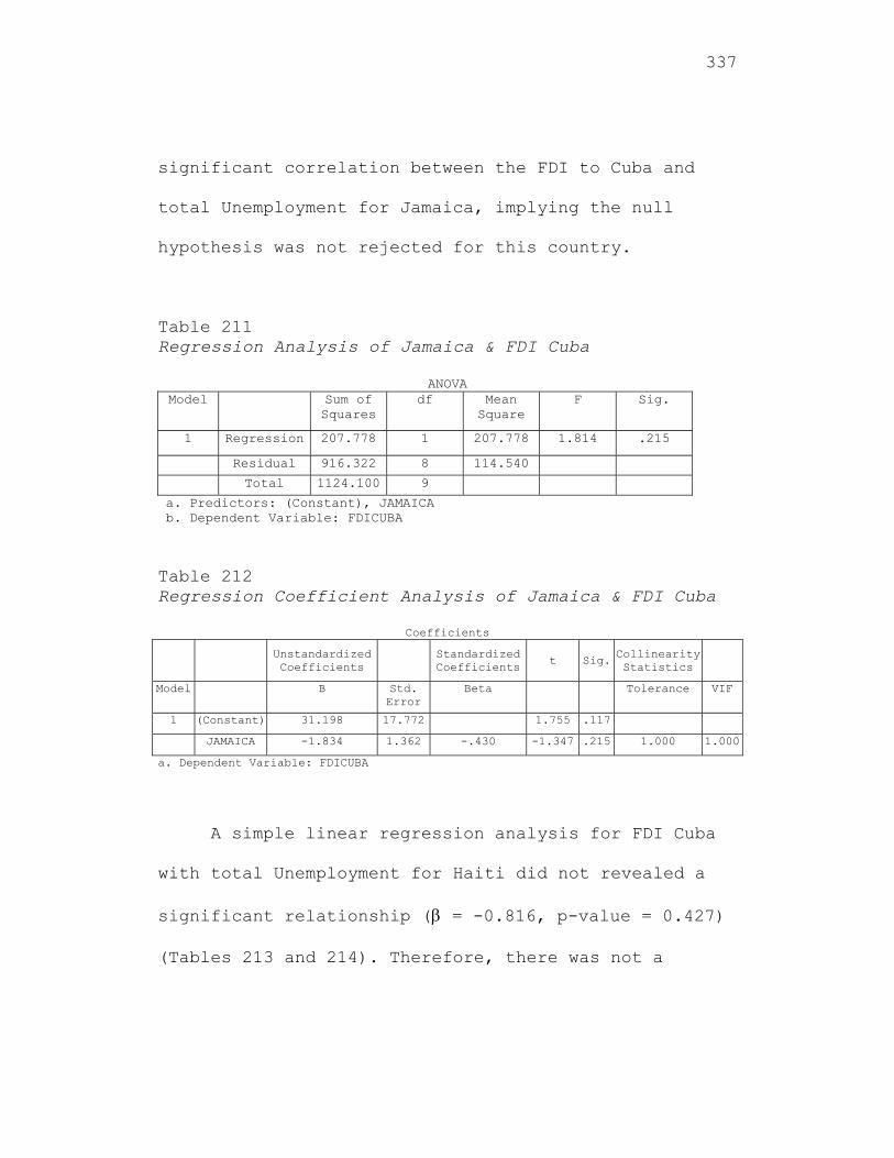
337

significant correlation between the FDI to Cuba and

total Unemployment for Jamaica, implying the null

hypothesis was not rejected for this country.

Table 211 Regression Analysis of Jamaica & FDI Cuba

ANOVA Model Sum of

Squares df Mean

Square F Sig.

1 Regression 207.778 1 207.778 1.814 .215

Residual 916.322 8 114.540

Total 1124.100 9

a. Predictors: (Constant), JAMAICA b. Dependent Variable: FDICUBA

Table 212 Regression Coefficient Analysis of Jamaica & FDI Cuba

Coefficients

Unstandardized Coefficients

Standardized Coefficients

t Sig. Collinearity Statistics

Model B Std. Error

Beta Tolerance VIF

1 (Constant) 31.198 17.772 1.755 .117

JAMAICA -1.834 1.362 -.430 -1.347 .215 1.000 1.000

a. Dependent Variable: FDICUBA

A simple linear regression analysis for FDI Cuba

with total Unemployment for Haiti did not revealed a

significant relationship ( = -0.816, p-value = 0.427)

(Tables 213 and 214). Therefore, there was not a

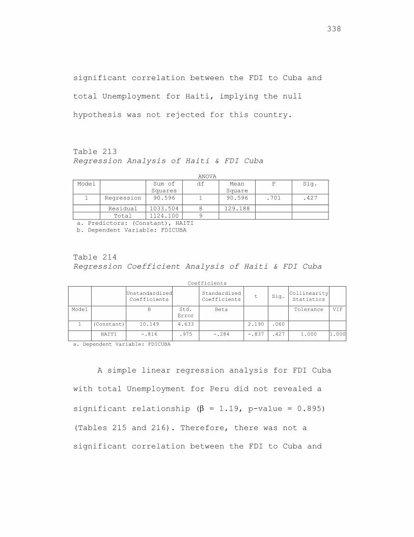
338

significant correlation between the FDI to Cuba and

total Unemployment for Haiti, implying the null

hypothesis was not rejected for this country.

Table 213 Regression Analysis of Haiti & FDI Cuba

ANOVA

Model Sum of Squares

df Mean Square

F Sig.

1 Regression 90.596 1 90.596 .701 .427

Residual 1033.504 8 129.188 Total 1124.100 9

a. Predictors: (Constant), HAITI b. Dependent Variable: FDICUBA

Table 214 Regression Coefficient Analysis of Haiti & FDI Cuba

Coefficients

Unstandardized Coefficients

Standardized Coefficients

t Sig. Collinearity Statistics

Model B Std. Error

Beta Tolerance VIF

1 (Constant) 10.149 4.633 2.190 .060

HAITI -.816 .975 -.284 -.837 .427 1.000 1.000

a. Dependent Variable: FDICUBA

A simple linear regression analysis for FDI Cuba

with total Unemployment for Peru did not revealed a

significant relationship ( = 1.19, p-value = 0.895)

(Tables 215 and 216). Therefore, there was not a

significant correlation between the FDI to Cuba and

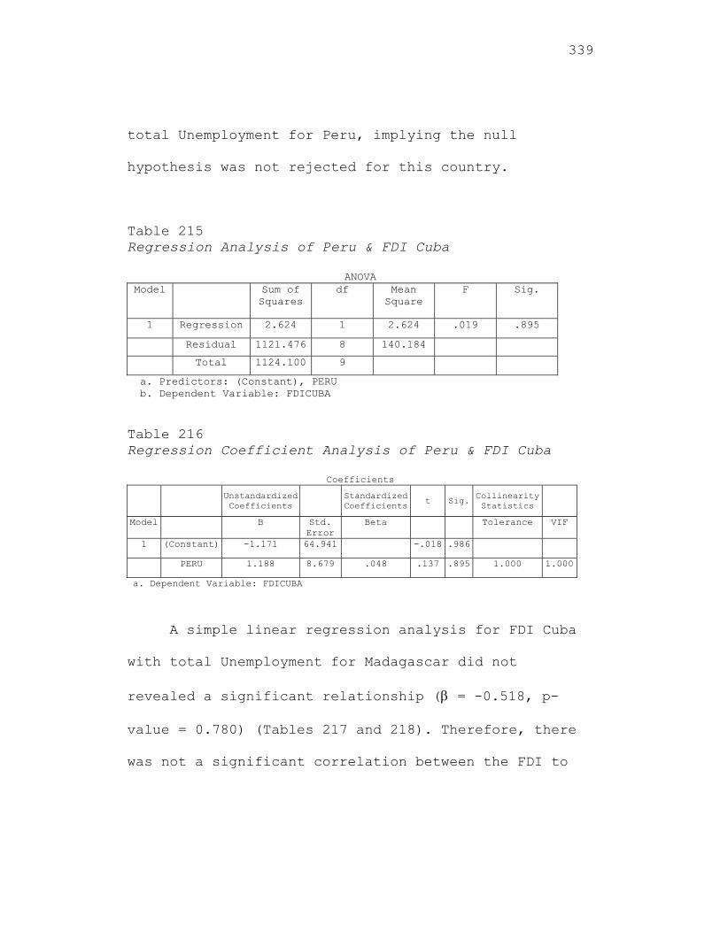
339

total Unemployment for Peru, implying the null

hypothesis was not rejected for this country.

Table 215 Regression Analysis of Peru & FDI Cuba

ANOVA Model Sum of

Squares df Mean

Square F Sig.

1 Regression 2.624 1 2.624 .019 .895

Residual 1121.476 8 140.184

Total 1124.100 9

a. Predictors: (Constant), PERU b. Dependent Variable: FDICUBA Table 216 Regression Coefficient Analysis of Peru & FDI Cuba

Coefficients Unstandardized

Coefficients

Standardized Coefficients

t Sig.Collinearity Statistics

Model B Std. Error

Beta Tolerance VIF

1 (Constant) -1.171 64.941 -.018 .986

PERU 1.188 8.679 .048 .137 .895 1.000 1.000

a. Dependent Variable: FDICUBA

A simple linear regression analysis for FDI Cuba

with total Unemployment for Madagascar did not

revealed a significant relationship ( = -0.518, p-

value = 0.780) (Tables 217 and 218). Therefore, there

was not a significant correlation between the FDI to

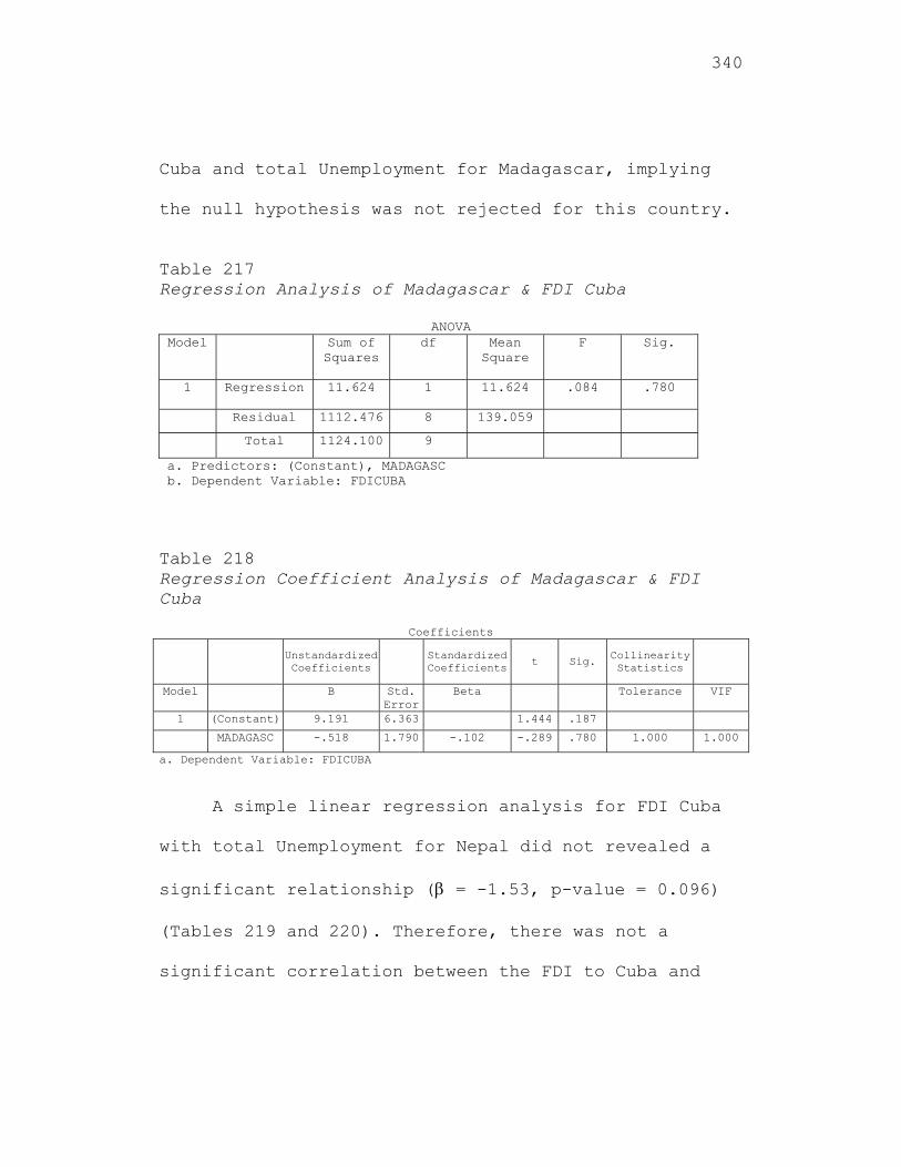
340

Cuba and total Unemployment for Madagascar, implying

the null hypothesis was not rejected for this country.

Table 217 Regression Analysis of Madagascar & FDI Cuba

ANOVA Model Sum of

Squares df Mean

Square F Sig.

1 Regression 11.624 1 11.624 .084 .780

Residual 1112.476 8 139.059

Total 1124.100 9

a. Predictors: (Constant), MADAGASC b. Dependent Variable: FDICUBA

Table 218 Regression Coefficient Analysis of Madagascar & FDI Cuba

Coefficients

Unstandardized Coefficients

Standardized Coefficients

t Sig. Collinearity Statistics

Model B Std. Error

Beta Tolerance VIF

1 (Constant) 9.191 6.363 1.444 .187

MADAGASC -.518 1.790 -.102 -.289 .780 1.000 1.000

a. Dependent Variable: FDICUBA

A simple linear regression analysis for FDI Cuba

with total Unemployment for Nepal did not revealed a

significant relationship ( = -1.53, p-value = 0.096)

(Tables 219 and 220). Therefore, there was not a

significant correlation between the FDI to Cuba and

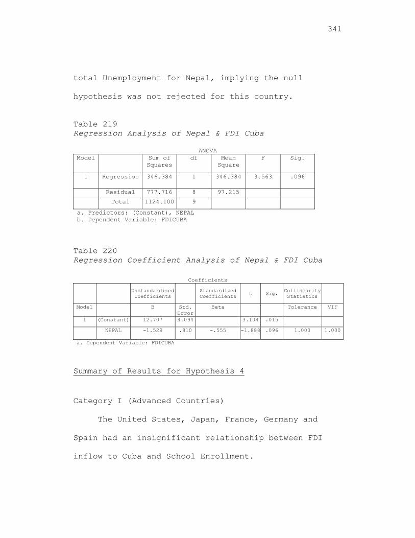
341

total Unemployment for Nepal, implying the null

hypothesis was not rejected for this country.

Table 219 Regression Analysis of Nepal & FDI Cuba

ANOVA Model Sum of

Squares df Mean

Square F Sig.

1 Regression 346.384 1 346.384 3.563 .096

Residual 777.716 8 97.215

Total 1124.100 9

a. Predictors: (Constant), NEPAL b. Dependent Variable: FDICUBA Table 220 Regression Coefficient Analysis of Nepal & FDI Cuba

Coefficients

Unstandardized Coefficients

Standardized Coefficients

t Sig. Collinearity Statistics

Model B Std. Error

Beta Tolerance VIF

1 (Constant) 12.707 4.094 3.104 .015

NEPAL -1.529 .810 -.555 -1.888 .096 1.000 1.000

a. Dependent Variable: FDICUBA

Summary of Results for Hypothesis 4

Category I (Advanced Countries)

The United States, Japan, France, Germany and

Spain had an insignificant relationship between FDI

inflow to Cuba and School Enrollment.

342

The United States, France, Germany and Spain had

an insignificant relationship between FDI inflow to

Cuba and total unemployment. Japan revealed a

significant negative relationship.

Category II (Developing Countries)

China, India and the Russian Federation had an

insignificant relationship between FDI inflow to Cuba

and School Enrollment.

China, India and the Russian Federation had an

insignificant relationship between FDI inflow to Cuba

and total Unemployment.

Category III (Least Developing Countries)

Significant positive correlation existed between

FDI inflow to Cuba and School Enrollment for Nepal.

Jamaica and Haiti revealed a significant negative

relationship. Insignificant result was found for Peru,

while Madagascar showed a marginally significant

positive relationship.

343

Jamaica, Haiti, Peru, Madagascar and Nepal had an

insignificant relationship between FDI inflow to Cuba

and total Unemployment.

Results for Hypothesis 5

FDI to Cuba was the dependent variable. For the

advanced countries, the independent variables were

Energy and Natural Resources for the United States,

Japan, Germany, France and Spain (Sawalha, 2007). The

independent variables for the developing countries

were Energy and Natural Resources for China, India and

the Russian Federation (Sawalha, 2007). The

independent variables for the Least Developed

Countries (LCD’s) were Energy and Natural Resources

for Jamaica, Haiti, Peru, Madagascar and Nepal. The

Republic of Cuba’s Energy and Natural Resources was

not included in the model as there were only three

data points. The Energy and Natural Resources

hypothesis included two variables, Energy Use

(measured in kilograms of oil equivalent per capita)

344

and Fuel Imports (measured as a percentage of

merchandise imports in United States dollars).

The fifth hypothesis to be tested is:

Hypothesis H05: The level of contribution of FDI

inflow to Cuba is not significantly related to

the Energy and Natural Resources for the three

groups of countries.

Hypothesis HA5: The level of contribution of FDI

inflow to Cuba is significantly related to the

Energy and Natural Resources for the three

groups of countries.

The multiple regression models to test Hypothesis 5

are listed below.

Category I (Advanced Countries)

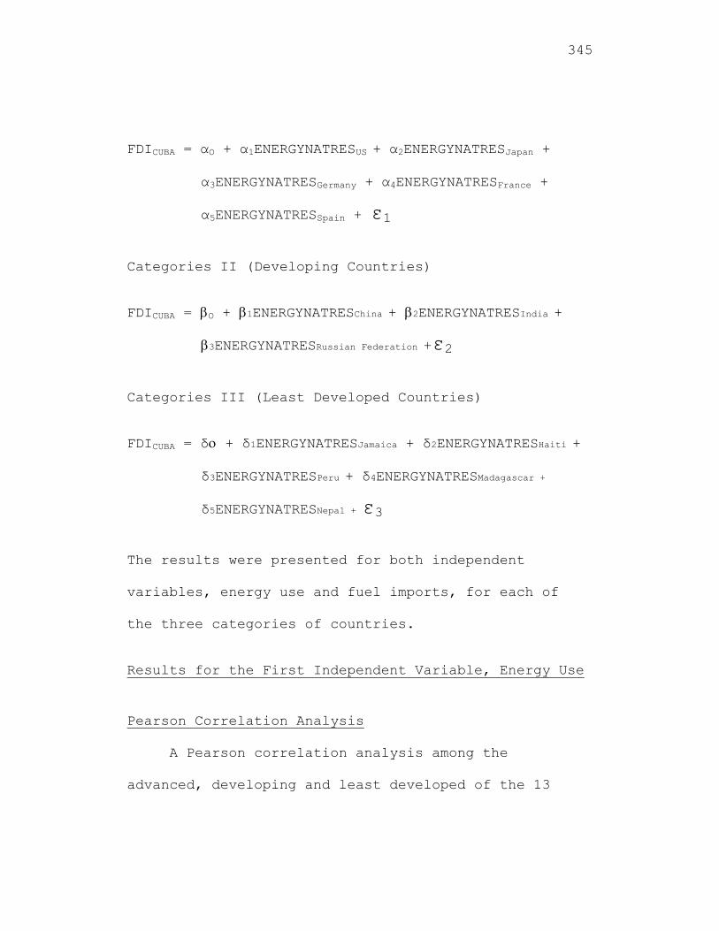
345

FDICUBA = αO + α1ENERGYNATRESUS + α2ENERGYNATRESJapan +

α3ENERGYNATRESGermany + α4ENERGYNATRESFrance +

α5ENERGYNATRESSpain + ε1

Categories II (Developing Countries)

FDICUBA = O + 1ENERGYNATRESChina + 2ENERGYNATRESIndia +

3ENERGYNATRESRussian Federation +ε2

Categories III (Least Developed Countries)

FDICUBA = δ + δ1ENERGYNATRESJamaica + δ2ENERGYNATRESHaiti +

δ3ENERGYNATRESPeru + δ4ENERGYNATRESMadagascar +

δ5ENERGYNATRESNepal + ε3

The results were presented for both independent

variables, energy use and fuel imports, for each of

the three categories of countries.

Results for the First Independent Variable, Energy Use

Pearson Correlation Analysis

A Pearson correlation analysis among the

advanced, developing and least developed of the 13

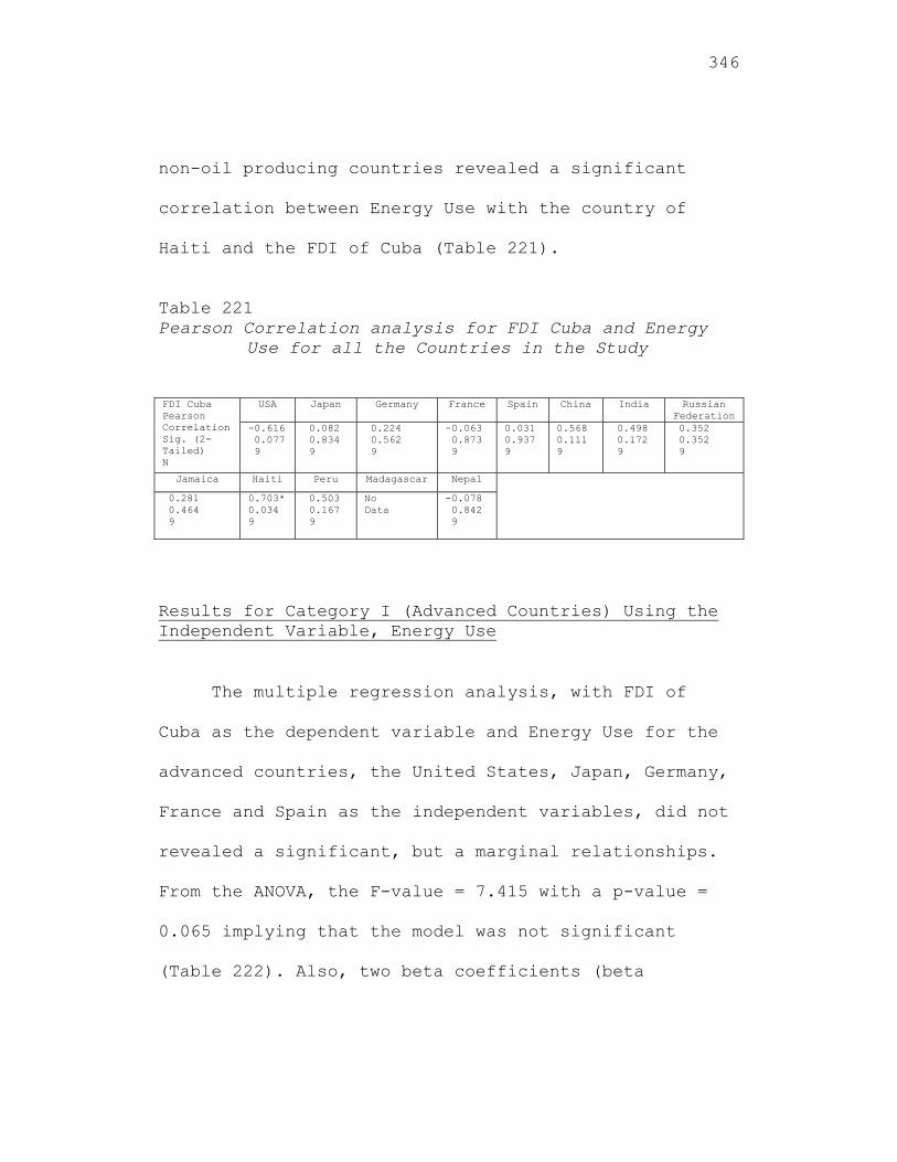
346

non-oil producing countries revealed a significant

correlation between Energy Use with the country of

Haiti and the FDI of Cuba (Table 221).

Table 221 Pearson Correlation analysis for FDI Cuba and Energy

Use for all the Countries in the Study FDI Cuba Pearson Correlation Sig. (2-Tailed) N

USA Japan Germany France Spain China India Russian Federation

-0.616 0.077 9

0.082 0.834 9

0.224 0.562 9

-0.063 0.873 9

0.031 0.937 9

0.568 0.111 9

0.498 0.172 9

0.352 0.352 9

Jamaica Haiti Peru Madagascar Nepal

0.281 0.464 9

0.703* 0.034 9

0.503 0.167 9

No Data

-0.078 0.842 9

Results for Category I (Advanced Countries) Using the Independent Variable, Energy Use

The multiple regression analysis, with FDI of

Cuba as the dependent variable and Energy Use for the

advanced countries, the United States, Japan, Germany,

France and Spain as the independent variables, did not

revealed a significant, but a marginal relationships.

From the ANOVA, the F-value = 7.415 with a p-value =

0.065 implying that the model was not significant

(Table 222). Also, two beta coefficients (beta

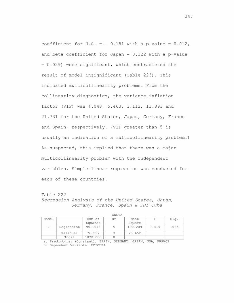
347

coefficient for U.S. = - 0.181 with a p-value = 0.012,

and beta coefficient for Japan = 0.322 with a p-value

= 0.029) were significant, which contradicted the

result of model insignificant (Table 223). This

indicated multicollinearity problems. From the

collinearity diagnostics, the variance inflation

factor (VIF) was 4.048, 5.463, 3.112, 11.893 and

21.731 for the United States, Japan, Germany, France

and Spain, respectively. (VIF greater than 5 is

usually an indication of a multicollinearity problem.)

As suspected, this implied that there was a major

multicollinearity problem with the independent

variables. Simple linear regression was conducted for

each of these countries.

Table 222 Regression Analysis of the United States, Japan,

Germany, France, Spain & FDI Cuba

ANOVA Model Sum of

Squares df Mean

Square F Sig.

1 Regression 951.043 5 190.209 7.415 .065

Residual 76.957 3 25.652 Total 1028.000 8

a. Predictors: (Constant), SPAIN, GERMANY, JAPAN, USA, FRANCE b. Dependent Variable: FDICUBA

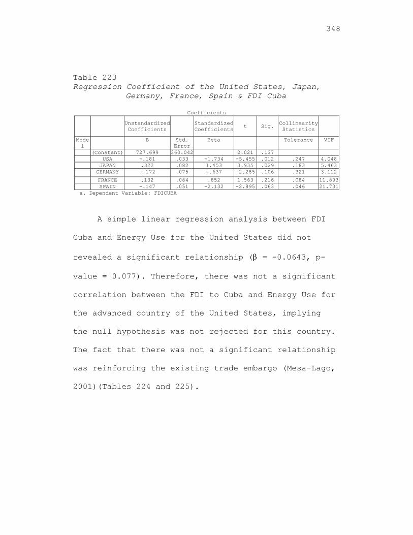
348

Table 223 Regression Coefficient of the United States, Japan,

Germany, France, Spain & FDI Cuba

Coefficients

Unstandardized Coefficients

Standardized Coefficients t Sig.

Collinearity Statistics

Model

B Std. Error

Beta Tolerance VIF

(Constant) 727.699 360.042 2.021 .137 USA -.181 .033 -1.734 -5.455 .012 .247 4.048 JAPAN .322 .082 1.453 3.935 .029 .183 5.463 GERMANY -.172 .075 -.637 -2.285 .106 .321 3.112

FRANCE .132 .084 .852 1.563 .216 .084 11.893 SPAIN -.147 .051 -2.132 -2.895 .063 .046 21.731

a. Dependent Variable: FDICUBA

A simple linear regression analysis between FDI

Cuba and Energy Use for the United States did not

revealed a significant relationship ( = -0.0643, p-

value = 0.077). Therefore, there was not a significant

correlation between the FDI to Cuba and Energy Use for

the advanced country of the United States, implying

the null hypothesis was not rejected for this country.

The fact that there was not a significant relationship

was reinforcing the existing trade embargo (Mesa-Lago,

2001)(Tables 224 and 225).

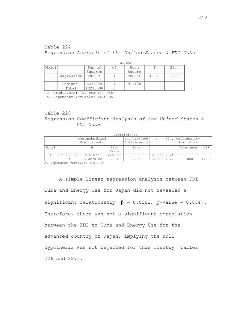
349

Table 224 Regression Analysis of the United States & FDI Cuba

ANOVA Model Sum of

Squaresdf Mean

Square F Sig.

1 Regression 390.091 1 390.091 4.281 .077

Residual 637.909 7 91.130 Total 1028.000 8

a. Predictors: (Constant), USA b. Dependent Variable: FDICUBA

Table 225 Regression Coefficient Analysis of the United States &

FDI Cuba

Coefficients Unstandardized

Coefficients Standardized

CoefficientsT Sig. Collinearity

Statistics

Model B Std. Error

Beta Tolerance VIF

1 (Constant) 516.677 246.526 2.096 .074 USA -6.427E-02 .031 -.616 -2.069 .077 1.000 1.000

a. Dependent Variable: FDICUBA

A simple linear regression analysis between FDI

Cuba and Energy Use for Japan did not revealed a

significant relationship ( = 0.0182, p-value = 0.834).

Therefore, there was not a significant correlation

between the FDI to Cuba and Energy Use for the

advanced country of Japan, implying the null

hypothesis was not rejected for this country (Tables

226 and 227).

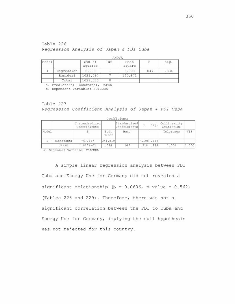
350

Table 226 Regression Analysis of Japan & FDI Cuba

ANOVA

Model Sum of Squares

df Mean Square

F Sig.

1 Regression 6.903 1 6.903 .047 .834 Residual 1021.097 7 145.871 Total 1028.000 8

a. Predictors: (Constant), JAPAN b. Dependent Variable: FDICUBA

Table 227 Regression Coefficient Analysis of Japan & FDI Cuba

Coefficients Unstandardized

Coefficients Standardized

Coefficientst Sig. Collinearity

Statistics

Model B Std. Error

Beta Tolerance VIF

1 (Constant) -67.687 341.819 -.198 .849

JAPAN 1.817E-02 .084 .082 .218 .834 1.000 1.000

a. Dependent Variable: FDICUBA

A simple linear regression analysis between FDI

Cuba and Energy Use for Germany did not revealed a

significant relationship ( = 0.0606, p-value = 0.562)

(Tables 228 and 229). Therefore, there was not a

significant correlation between the FDI to Cuba and

Energy Use for Germany, implying the null hypothesis

was not rejected for this country.

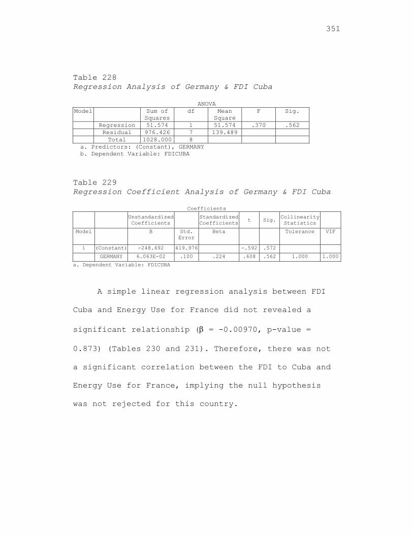
351

Table 228 Regression Analysis of Germany & FDI Cuba

ANOVA Model Sum of

Squares df Mean

Square F Sig.

Regression 51.574 1 51.574 .370 .562 Residual 976.426 7 139.489 Total 1028.000 8

a. Predictors: (Constant), GERMANY b. Dependent Variable: FDICUBA Table 229 Regression Coefficient Analysis of Germany & FDI Cuba

Coefficients Unstandardized

Coefficients Standardized

Coefficientst Sig. Collinearity

Statistics

Model B Std. Error

Beta Tolerance VIF

1 (Constant) -248.692 419.976 -.592 .572

GERMANY 6.063E-02 .100 .224 .608 .562 1.000 1.000

a. Dependent Variable: FDICUBA

A simple linear regression analysis between FDI

Cuba and Energy Use for France did not revealed a

significant relationship ( = -0.00970, p-value =

0.873) (Tables 230 and 231). Therefore, there was not

a significant correlation between the FDI to Cuba and

Energy Use for France, implying the null hypothesis

was not rejected for this country.

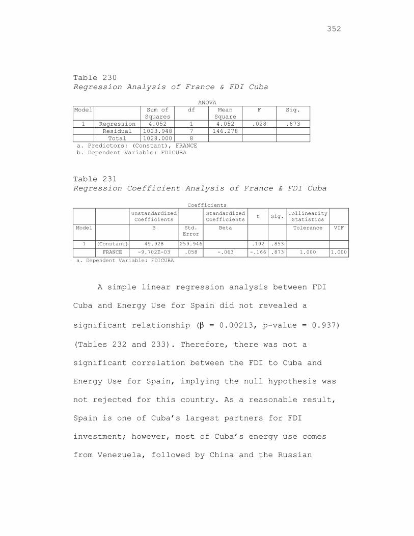
352

Table 230 Regression Analysis of France & FDI Cuba

ANOVA Model Sum of

Squares df Mean

Square F Sig.

1 Regression 4.052 1 4.052 .028 .873 Residual 1023.948 7 146.278 Total 1028.000 8

a. Predictors: (Constant), FRANCE b. Dependent Variable: FDICUBA

Table 231 Regression Coefficient Analysis of France & FDI Cuba

Coefficients Unstandardized

Coefficients Standardized

Coefficientst Sig. Collinearity

Statistics

Model B Std. Error

Beta Tolerance VIF

1 (Constant) 49.928 259.946 .192 .853

FRANCE -9.702E-03 .058 -.063 -.166 .873 1.000 1.000

a. Dependent Variable: FDICUBA

A simple linear regression analysis between FDI

Cuba and Energy Use for Spain did not revealed a

significant relationship ( = 0.00213, p-value = 0.937)

(Tables 232 and 233). Therefore, there was not a

significant correlation between the FDI to Cuba and

Energy Use for Spain, implying the null hypothesis was

not rejected for this country. As a reasonable result,

Spain is one of Cuba’s largest partners for FDI

investment; however, most of Cuba’s energy use comes

from Venezuela, followed by China and the Russian

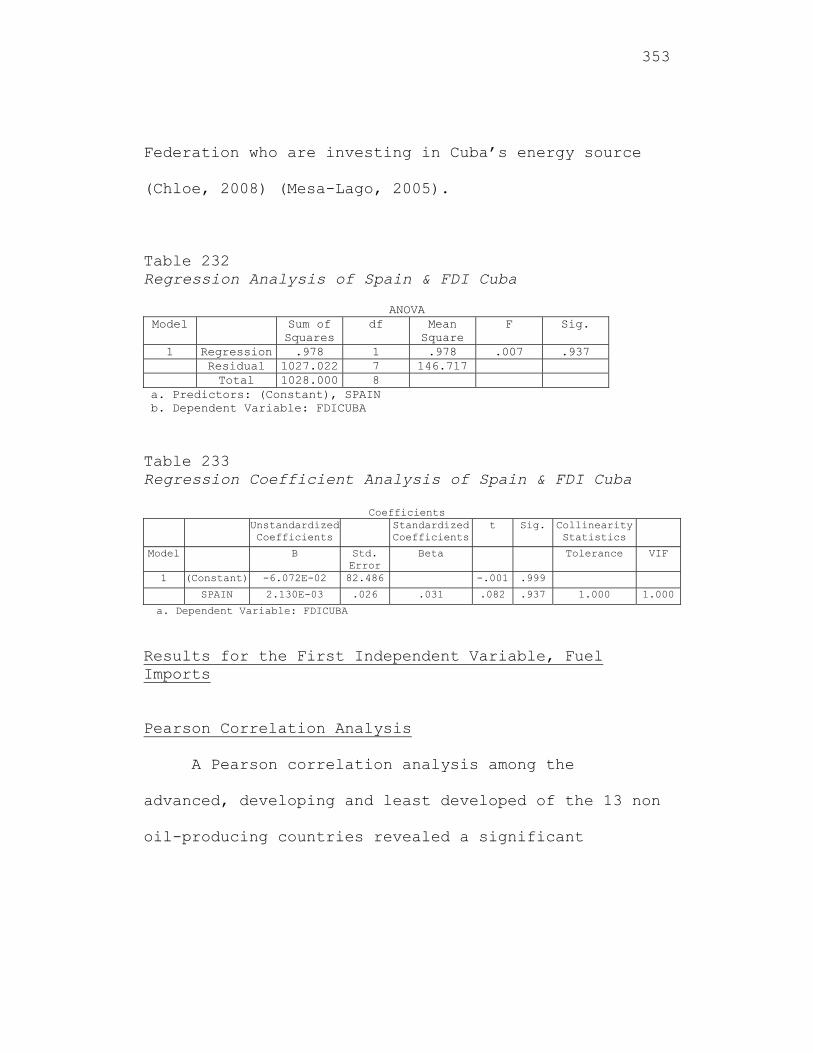
353

Federation who are investing in Cuba’s energy source

(Chloe, 2008) (Mesa-Lago, 2005).

Table 232 Regression Analysis of Spain & FDI Cuba

ANOVA

Model Sum of Squares

df Mean Square

F Sig.

1 Regression .978 1 .978 .007 .937 Residual 1027.022 7 146.717 Total 1028.000 8

a. Predictors: (Constant), SPAIN b. Dependent Variable: FDICUBA

Table 233 Regression Coefficient Analysis of Spain & FDI Cuba

Coefficients Unstandardized

Coefficients Standardized

Coefficientst Sig. Collinearity

Statistics

Model B Std. Error

Beta Tolerance VIF

1 (Constant) -6.072E-02 82.486 -.001 .999

SPAIN 2.130E-03 .026 .031 .082 .937 1.000 1.000

a. Dependent Variable: FDICUBA

Results for the First Independent Variable, Fuel Imports

Pearson Correlation Analysis

A Pearson correlation analysis among the

advanced, developing and least developed of the 13 non

oil-producing countries revealed a significant

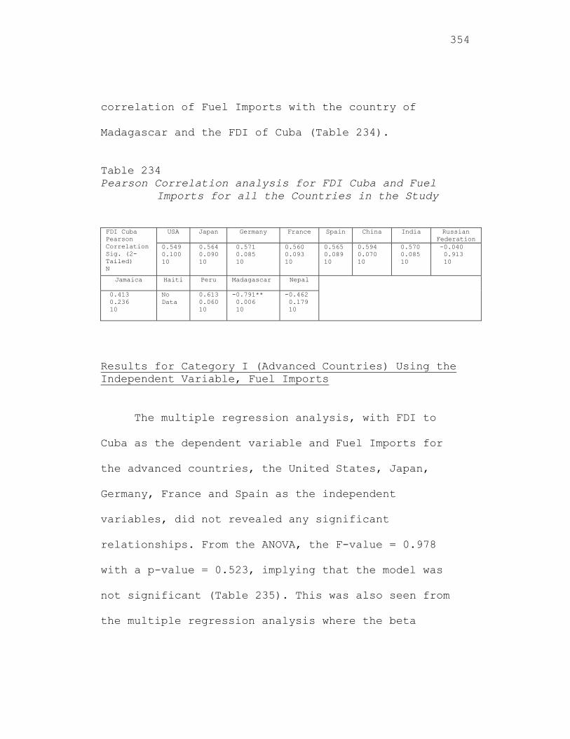
354

correlation of Fuel Imports with the country of

Madagascar and the FDI of Cuba (Table 234).

Table 234 Pearson Correlation analysis for FDI Cuba and Fuel

Imports for all the Countries in the Study FDI Cuba Pearson Correlation Sig. (2-Tailed) N

USA Japan Germany France Spain China India Russian Federation

0.549 0.100 10

0.564 0.090 10

0.571 0.085 10

0.560 0.093 10

0.565 0.089 10

0.594 0.070 10

0.570 0.085 10

-0.040 0.913 10

Jamaica Haiti Peru Madagascar Nepal

0.413 0.236 10

No Data

0.613 0.060 10

-0.791** 0.006 10

-0.462 0.179 10

Results for Category I (Advanced Countries) Using the Independent Variable, Fuel Imports

The multiple regression analysis, with FDI to

Cuba as the dependent variable and Fuel Imports for

the advanced countries, the United States, Japan,

Germany, France and Spain as the independent

variables, did not revealed any significant

relationships. From the ANOVA, the F-value = 0.978

with a p-value = 0.523, implying that the model was

not significant (Table 235). This was also seen from

the multiple regression analysis where the beta

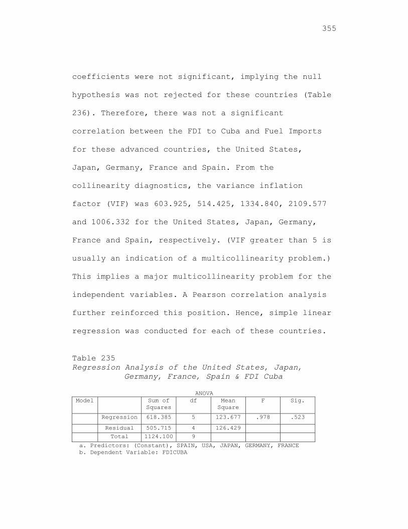
355

coefficients were not significant, implying the null

hypothesis was not rejected for these countries (Table

236). Therefore, there was not a significant

correlation between the FDI to Cuba and Fuel Imports

for these advanced countries, the United States,

Japan, Germany, France and Spain. From the

collinearity diagnostics, the variance inflation

factor (VIF) was 603.925, 514.425, 1334.840, 2109.577

and 1006.332 for the United States, Japan, Germany,

France and Spain, respectively. (VIF greater than 5 is

usually an indication of a multicollinearity problem.)

This implies a major multicollinearity problem for the

independent variables. A Pearson correlation analysis

further reinforced this position. Hence, simple linear

regression was conducted for each of these countries.

Table 235 Regression Analysis of the United States, Japan,

Germany, France, Spain & FDI Cuba

ANOVA Model Sum of

Squares df Mean

Square F Sig.

Regression 618.385 5 123.677 .978 .523

Residual 505.715 4 126.429 Total 1124.100 9

a. Predictors: (Constant), SPAIN, USA, JAPAN, GERMANY, FRANCE b. Dependent Variable: FDICUBA

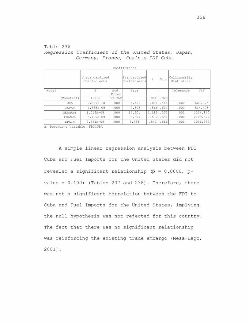
356

Table 236 Regression Coefficient of the United States, Japan,

Germany, France, Spain & FDI Cuba

Coefficients

Unstandardized Coefficients

Standardized Coefficients t Sig.

Collinearity Statistics

Model B Std. Error

Beta Tolerance VIF

(Constant) 1.866 19.762 .094 .929

USA -9.889E-10 .000 -6.598 -.801 .468 .002 603.925

JAPAN -1.655E-09 .000 -4.308 -.566 .601 .002 514.425

GERMANY 1.015E-08 .000 14.501 1.183 .302 .001 1334.840 FRANCE -8.109E-09 .000 -8.807 -.572 .598 .000 2109.577

SPAIN 7.561E-09 .000 5.768 .542 .616 .001 1006.332

a. Dependent Variable: FDICUBA

A simple linear regression analysis between FDI

Cuba and Fuel Imports for the United States did not

revealed a significant relationship ( = 0.0000, p-

value = 0.100) (Tables 237 and 238). Therefore, there

was not a significant correlation between the FDI to

Cuba and Fuel Imports for the United States, implying

the null hypothesis was not rejected for this country.

The fact that there was no significant relationship

was reinforcing the existing trade embargo (Mesa-Lago,

2001).

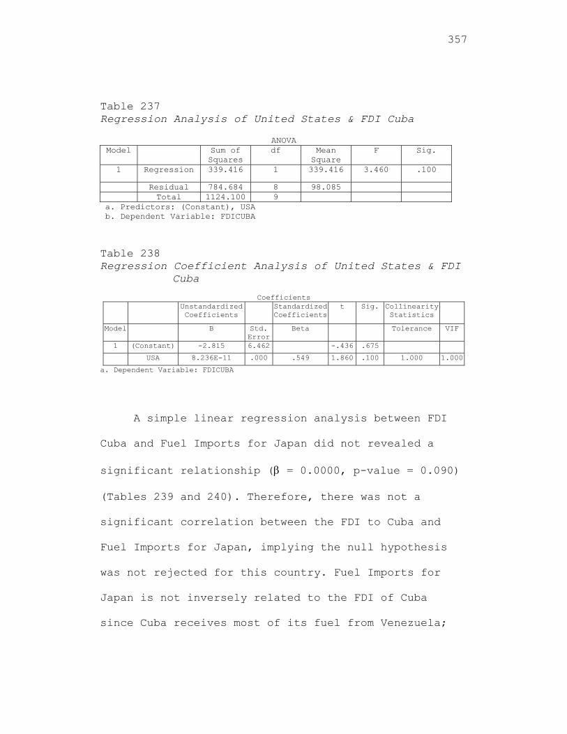
357

Table 237 Regression Analysis of United States & FDI Cuba

ANOVA Model Sum of

Squares df Mean

Square F Sig.

1 Regression 339.416 1 339.416 3.460 .100

Residual 784.684 8 98.085 Total 1124.100 9

a. Predictors: (Constant), USA b. Dependent Variable: FDICUBA

Table 238 Regression Coefficient Analysis of United States & FDI

Cuba

Coefficients Unstandardized

Coefficients Standardized

Coefficientst Sig. Collinearity

Statistics

Model B Std. Error

Beta Tolerance VIF

1 (Constant) -2.815 6.462 -.436 .675

USA 8.236E-11 .000 .549 1.860 .100 1.000 1.000

a. Dependent Variable: FDICUBA

A simple linear regression analysis between FDI

Cuba and Fuel Imports for Japan did not revealed a

significant relationship ( = 0.0000, p-value = 0.090)

(Tables 239 and 240). Therefore, there was not a

significant correlation between the FDI to Cuba and

Fuel Imports for Japan, implying the null hypothesis

was not rejected for this country. Fuel Imports for

Japan is not inversely related to the FDI of Cuba

since Cuba receives most of its fuel from Venezuela;

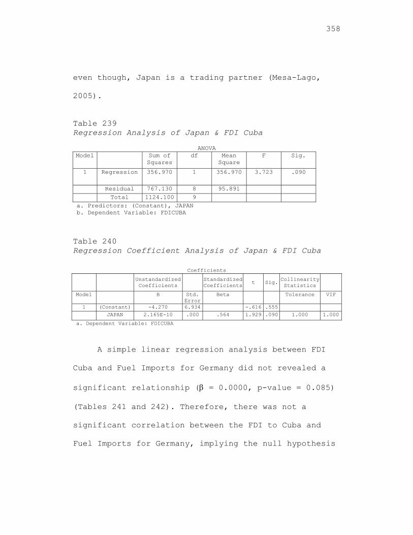
358

even though, Japan is a trading partner (Mesa-Lago,

2005).

Table 239 Regression Analysis of Japan & FDI Cuba

ANOVA

Model Sum of Squares

df Mean Square

F Sig.

1 Regression 356.970 1 356.970 3.723 .090

Residual 767.130 8 95.891 Total 1124.100 9

a. Predictors: (Constant), JAPAN b. Dependent Variable: FDICUBA

Table 240 Regression Coefficient Analysis of Japan & FDI Cuba

Coefficients

Unstandardized Coefficients

Standardized Coefficients

t Sig. Collinearity Statistics

Model B Std. Error

Beta Tolerance VIF

1 (Constant) -4.270 6.934 -.616 .555 JAPAN 2.165E-10 .000 .564 1.929 .090 1.000 1.000

a. Dependent Variable: FDICUBA

A simple linear regression analysis between FDI

Cuba and Fuel Imports for Germany did not revealed a

significant relationship ( = 0.0000, p-value = 0.085)

(Tables 241 and 242). Therefore, there was not a

significant correlation between the FDI to Cuba and

Fuel Imports for Germany, implying the null hypothesis

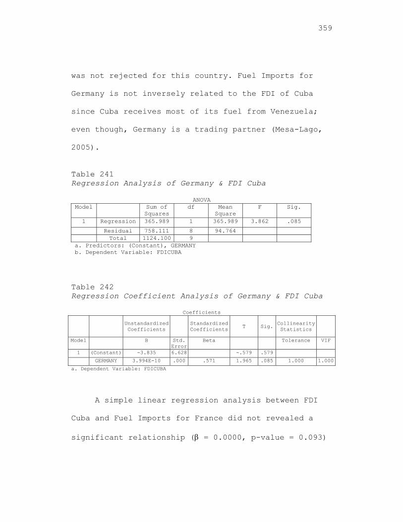
359

was not rejected for this country. Fuel Imports for

Germany is not inversely related to the FDI of Cuba

since Cuba receives most of its fuel from Venezuela;

even though, Germany is a trading partner (Mesa-Lago,

2005).

Table 241 Regression Analysis of Germany & FDI Cuba

ANOVA Model Sum of

Squares df Mean

Square F Sig.

1 Regression 365.989 1 365.989 3.862 .085

Residual 758.111 8 94.764 Total 1124.100 9

a. Predictors: (Constant), GERMANY b. Dependent Variable: FDICUBA

Table 242 Regression Coefficient Analysis of Germany & FDI Cuba

Coefficients

Unstandardized Coefficients

Standardized Coefficients T Sig.

Collinearity Statistics

Model B Std. Error

Beta Tolerance VIF

1 (Constant) -3.835 6.628 -.579 .579

GERMANY 3.994E-10 .000 .571 1.965 .085 1.000 1.000

a. Dependent Variable: FDICUBA

A simple linear regression analysis between FDI

Cuba and Fuel Imports for France did not revealed a

significant relationship ( = 0.0000, p-value = 0.093)

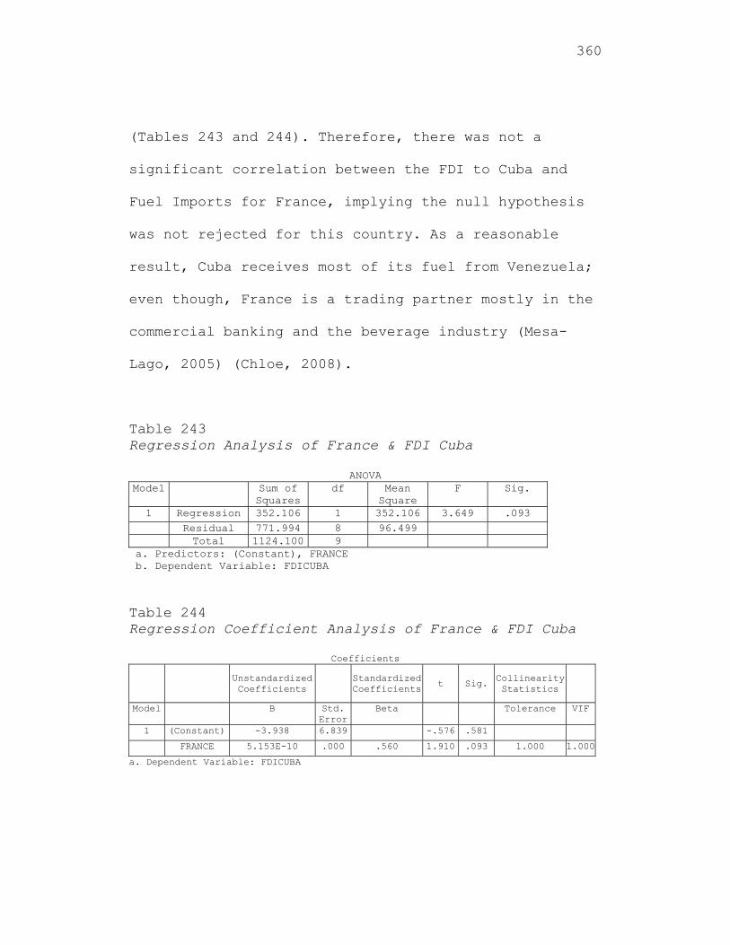
360

(Tables 243 and 244). Therefore, there was not a

significant correlation between the FDI to Cuba and

Fuel Imports for France, implying the null hypothesis

was not rejected for this country. As a reasonable

result, Cuba receives most of its fuel from Venezuela;

even though, France is a trading partner mostly in the

commercial banking and the beverage industry (Mesa-

Lago, 2005) (Chloe, 2008).

Table 243 Regression Analysis of France & FDI Cuba

ANOVA Model Sum of

Squares df Mean

Square F Sig.

1 Regression 352.106 1 352.106 3.649 .093 Residual 771.994 8 96.499 Total 1124.100 9

a. Predictors: (Constant), FRANCE b. Dependent Variable: FDICUBA

Table 244 Regression Coefficient Analysis of France & FDI Cuba

Coefficients

Unstandardized Coefficients

Standardized Coefficients

t Sig. Collinearity Statistics

Model B Std. Error

Beta Tolerance VIF

1 (Constant) -3.938 6.839 -.576 .581

FRANCE 5.153E-10 .000 .560 1.910 .093 1.000 1.000

a. Dependent Variable: FDICUBA

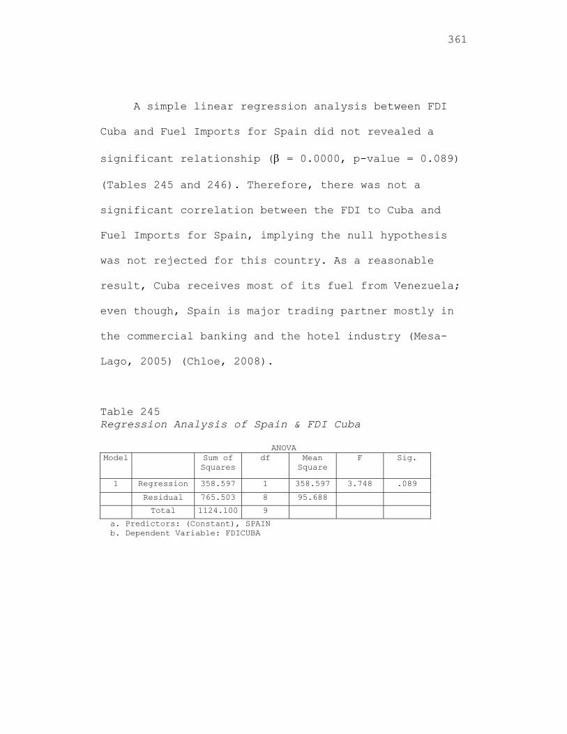
361

A simple linear regression analysis between FDI

Cuba and Fuel Imports for Spain did not revealed a

significant relationship ( = 0.0000, p-value = 0.089)

(Tables 245 and 246). Therefore, there was not a

significant correlation between the FDI to Cuba and

Fuel Imports for Spain, implying the null hypothesis

was not rejected for this country. As a reasonable

result, Cuba receives most of its fuel from Venezuela;

even though, Spain is major trading partner mostly in

the commercial banking and the hotel industry (Mesa-

Lago, 2005) (Chloe, 2008).

Table 245 Regression Analysis of Spain & FDI Cuba

ANOVA Model Sum of

Squares df Mean

Square F Sig.

1 Regression 358.597 1 358.597 3.748 .089

Residual 765.503 8 95.688

Total 1124.100 9

a. Predictors: (Constant), SPAIN b. Dependent Variable: FDICUBA

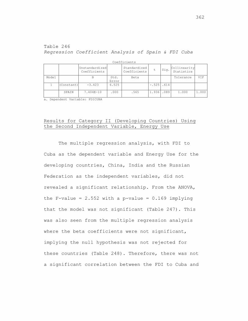
362

Table 246 Regression Coefficient Analysis of Spain & FDI Cuba

Coefficients

Unstandardized Coefficients

Standardized Coefficients t Sig.

Collinearity Statistics

Model B Std. Error

Beta Tolerance VIF

1 (Constant) -3.423 6.525 -.525 .614

SPAIN 7.404E-10 .000 .565 1.936 .089 1.000 1.000

a. Dependent Variable: FDICUBA

Results for Category II (Developing Countries) Using the Second Independent Variable, Energy Use

The multiple regression analysis, with FDI to

Cuba as the dependent variable and Energy Use for the

developing countries, China, India and the Russian

Federation as the independent variables, did not

revealed a significant relationship. From the ANOVA,

the F-value = 2.552 with a p-value = 0.169 implying

that the model was not significant (Table 247). This

was also seen from the multiple regression analysis

where the beta coefficients were not significant,

implying the null hypothesis was not rejected for

these countries (Table 248). Therefore, there was not

a significant correlation between the FDI to Cuba and

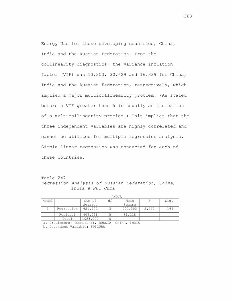
363

Energy Use for these developing countries, China,

India and the Russian Federation. From the

collinearity diagnostics, the variance inflation

factor (VIF) was 13.253, 30.629 and 16.339 for China,

India and the Russian Federation, respectively, which

implied a major multicollinearity problem. (As stated

before a VIF greater than 5 is usually an indication

of a multicollinearity problem.) This implies that the

three independent variables are highly correlated and

cannot be utilized for multiple regression analysis.

Simple linear regression was conducted for each of

these countries.

Table 247 Regression Analysis of Russian Federation, China,

India & FDI Cuba

ANOVA Model Sum of

Squares df Mean

Square F Sig.

1 Regression 621.909 3 207.303 2.552 .169

Residual 406.091 5 81.218 Total 1028.000 8

a. Predictors: (Constant), RUSSIA, CHINA, INDIA b. Dependent Variable: FDICUBA

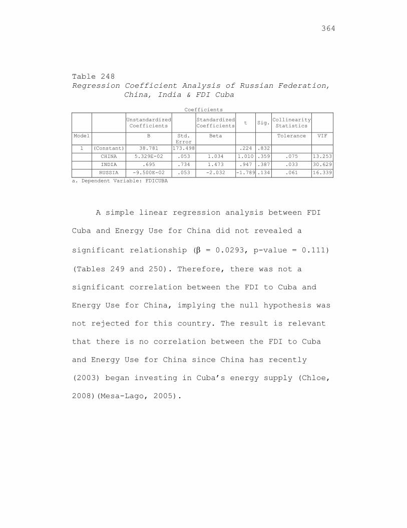
364

Table 248 Regression Coefficient Analysis of Russian Federation,

China, India & FDI Cuba

Coefficients

Unstandardized Coefficients

Standardized Coefficients

t Sig.Collinearity Statistics

Model B Std. Error

Beta Tolerance VIF

1 (Constant) 38.781 173.498 .224 .832

CHINA 5.329E-02 .053 1.034 1.010 .359 .075 13.253

INDIA .695 .734 1.473 .947 .387 .033 30.629

RUSSIA -9.500E-02 .053 -2.032 -1.789 .134 .061 16.339

a. Dependent Variable: FDICUBA

A simple linear regression analysis between FDI

Cuba and Energy Use for China did not revealed a

significant relationship ( = 0.0293, p-value = 0.111)

(Tables 249 and 250). Therefore, there was not a

significant correlation between the FDI to Cuba and

Energy Use for China, implying the null hypothesis was

not rejected for this country. The result is relevant

that there is no correlation between the FDI to Cuba

and Energy Use for China since China has recently

(2003) began investing in Cuba’s energy supply (Chloe,

2008)(Mesa-Lago, 2005).

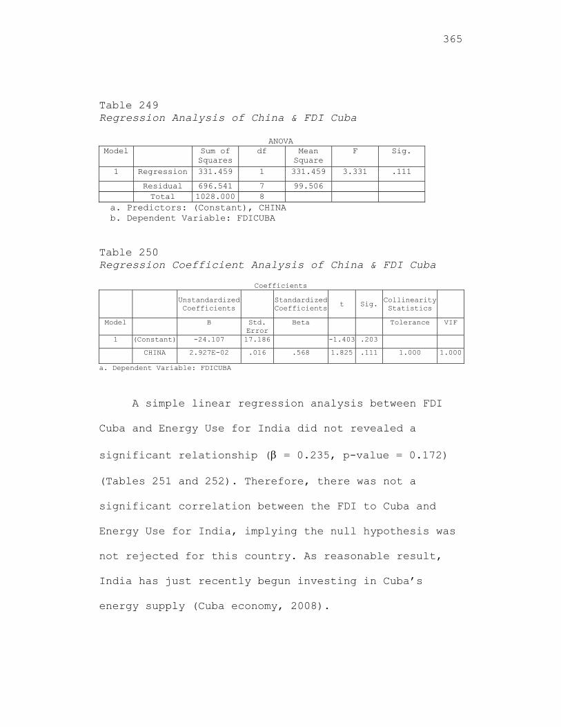
365

Table 249 Regression Analysis of China & FDI Cuba

ANOVA Model Sum of

Squares df Mean

Square F Sig.

1 Regression 331.459 1 331.459 3.331 .111

Residual 696.541 7 99.506 Total 1028.000 8

a. Predictors: (Constant), CHINA b. Dependent Variable: FDICUBA Table 250 Regression Coefficient Analysis of China & FDI Cuba

Coefficients

Unstandardized Coefficients

Standardized Coefficients

t Sig. Collinearity Statistics

Model B Std. Error

Beta Tolerance VIF

1 (Constant) -24.107 17.186 -1.403 .203

CHINA 2.927E-02 .016 .568 1.825 .111 1.000 1.000

a. Dependent Variable: FDICUBA

A simple linear regression analysis between FDI

Cuba and Energy Use for India did not revealed a

significant relationship ( = 0.235, p-value = 0.172)

(Tables 251 and 252). Therefore, there was not a

significant correlation between the FDI to Cuba and

Energy Use for India, implying the null hypothesis was

not rejected for this country. As reasonable result,

India has just recently begun investing in Cuba’s

energy supply (Cuba economy, 2008).

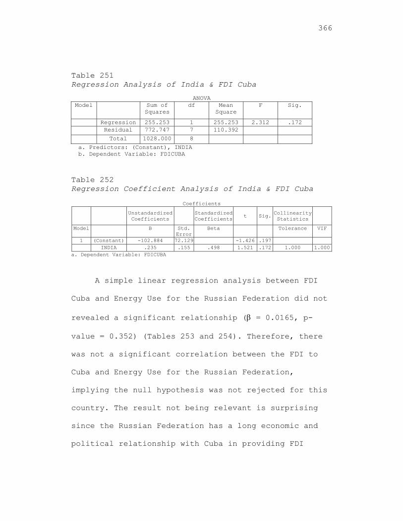
366

Table 251 Regression Analysis of India & FDI Cuba

ANOVA Model Sum of

Squares df Mean

Square F Sig.

Regression 255.253 1 255.253 2.312 .172 Residual 772.747 7 110.392

Total 1028.000 8

a. Predictors: (Constant), INDIA b. Dependent Variable: FDICUBA

Table 252 Regression Coefficient Analysis of India & FDI Cuba

Coefficients

Unstandardized Coefficients

Standardized Coefficients

t Sig. Collinearity Statistics

Model B Std. Error

Beta Tolerance VIF

1 (Constant) -102.884 72.129 -1.426 .197 INDIA .235 .155 .498 1.521 .172 1.000 1.000

a. Dependent Variable: FDICUBA

A simple linear regression analysis between FDI

Cuba and Energy Use for the Russian Federation did not

revealed a significant relationship ( = 0.0165, p-

value = 0.352) (Tables 253 and 254). Therefore, there

was not a significant correlation between the FDI to

Cuba and Energy Use for the Russian Federation,

implying the null hypothesis was not rejected for this

country. The result not being relevant is surprising

since the Russian Federation has a long economic and

political relationship with Cuba in providing FDI

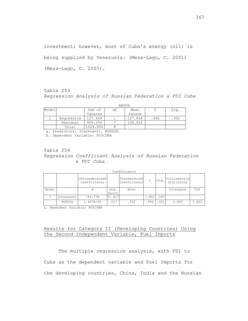
367

investment; however, most of Cuba’s energy (oil) is

being supplied by Venezuela. (Mesa-Lago, C. 2001)

(Mesa-Lago, C. 2005).

Table 253 Regression Analysis of Russian Federation & FDI Cuba

ANOVA Model Sum of

Squares df Mean

Square F Sig.

1 Regression 127.644 1 127.644 .992 .352 Residual 900.356 7 128.622 Total 1028.000 8

a. Predictors: (Constant), RUSSIA b. Dependent Variable: FDICUBA Table 254 Regression Coefficient Analysis of Russian Federation

& FDI Cuba

Coefficients

Unstandardized Coefficients

Standardized Coefficients t Sig.

Collinearity Statistics

Model B Std. Error

Beta Tolerance VIF

1 (Constant) -64.778 71.817 -.902 .397

RUSSIA 1.647E-02 .017 .352 .996 .352 1.000 1.000

a. Dependent Variable: FDICUBA

Results for Category II (Developing Countries) Using the Second Independent Variable, Fuel Imports

The multiple regression analysis, with FDI to

Cuba as the dependent variable and Fuel Imports for

the developing countries, China, India and the Russian

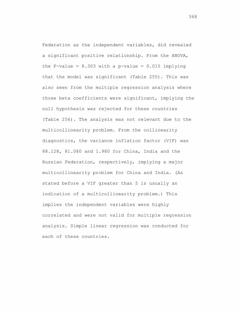
368

Federation as the independent variables, did revealed

a significant positive relationship. From the ANOVA,

the F-value = 8.303 with a p-value = 0.015 implying

that the model was significant (Table 255). This was

also seen from the multiple regression analysis where

three beta coefficients were significant, implying the

null hypothesis was rejected for these countries

(Table 256). The analysis was not relevant due to the

multicollinearity problem. From the collinearity

diagnostics, the variance inflation factor (VIF) was

88.128, 81.080 and 1.980 for China, India and the

Russian Federation, respectively, implying a major

multicollinearity problem for China and India. (As

stated before a VIF greater than 5 is usually an

indication of a multicollinearity problem.) This

implies the independent variables were highly

correlated and were not valid for multiple regression

analysis. Simple linear regression was conducted for

each of these countries.

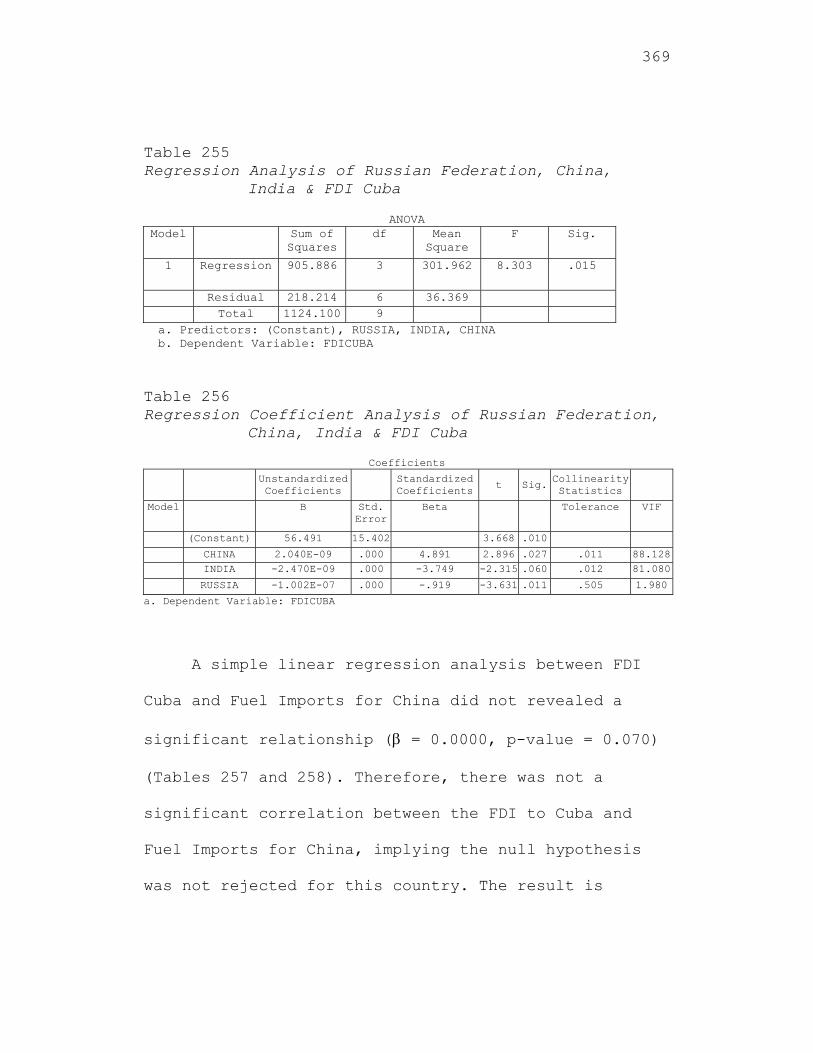
369

Table 255 Regression Analysis of Russian Federation, China,

India & FDI Cuba

ANOVA Model Sum of

Squares df Mean

Square F Sig.

1 Regression 905.886 3 301.962 8.303 .015

Residual 218.214 6 36.369 Total 1124.100 9

a. Predictors: (Constant), RUSSIA, INDIA, CHINA b. Dependent Variable: FDICUBA

Table 256 Regression Coefficient Analysis of Russian Federation,

China, India & FDI Cuba

Coefficients Unstandardized

Coefficients Standardized Coefficients t Sig.

Collinearity Statistics

Model B Std. Error

Beta Tolerance VIF

(Constant) 56.491 15.402 3.668 .010

CHINA 2.040E-09 .000 4.891 2.896 .027 .011 88.128 INDIA -2.470E-09 .000 -3.749 -2.315 .060 .012 81.080

RUSSIA -1.002E-07 .000 -.919 -3.631 .011 .505 1.980

a. Dependent Variable: FDICUBA

A simple linear regression analysis between FDI

Cuba and Fuel Imports for China did not revealed a

significant relationship ( = 0.0000, p-value = 0.070)

(Tables 257 and 258). Therefore, there was not a

significant correlation between the FDI to Cuba and

Fuel Imports for China, implying the null hypothesis

was not rejected for this country. The result is

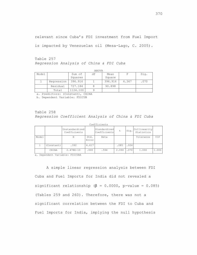
370

relevant since Cuba’s FDI investment from Fuel Import

is impacted by Venezuelan oil (Mesa-Lago, C. 2005).

Table 257 Regression Analysis of China & FDI Cuba

ANOVA Model Sum of

Squares df Mean

Square F Sig.

1 Regression 396.916 1 396.916 4.367 .070

Residual 727.184 8 90.898 Total 1124.100 9

a. Predictors: (Constant), CHINA b. Dependent Variable: FDICUB

Table 258 Regression Coefficient Analysis of China & FDI Cuba

Coefficients

Unstandardized Coefficients

Standardized Coefficients

t Sig. Collinearity Statistics

Model B Std. Error

Beta Tolerance VIF

1 (Constant) .392 4.617 .085 .934

CHINA 2.478E-10 .000 .594 2.090 .070 1.000 1.000

a. Dependent Variable: FDICUBA

A simple linear regression analysis between FDI

Cuba and Fuel Imports for India did not revealed a

significant relationship ( = 0.0000, p-value = 0.085)

(Tables 259 and 260). Therefore, there was not a

significant correlation between the FDI to Cuba and

Fuel Imports for India, implying the null hypothesis

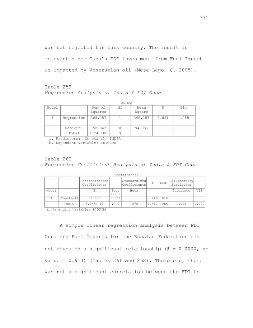
371

was not rejected for this country. The result is

relevant since Cuba’s FDI investment from Fuel Import

is impacted by Venezuelan oil (Mesa-Lago, C. 2005).

Table 259 Regression Analysis of India & FDI Cuba

ANOVA Model Sum of

Squares df Mean

Square F Sig.

1 Regression 365.257 1 365.257 3.851 .085

Residual 758.843 8 94.855 Total 1124.100 9

a. Predictors: (Constant), INDIA b. Dependent Variable: FDICUBA

Table 260 Regression Coefficient Analysis of India & FDI Cuba

Coefficients

Unstandardized Coefficients

Standardized Coefficients t Sig.

Collinearity Statistics

Model B Std. Error

Beta Tolerance VIF

1 (Constant) -1.386 5.561 -.249 .810

INDIA 3.756E-10 .000 .570 1.962 .085 1.000 1.000

a. Dependent Variable: FDICUBA

A simple linear regression analysis between FDI

Cuba and Fuel Imports for the Russian Federation did

not revealed a significant relationship ( = 0.0000, p-

value = 0.913) (Tables 261 and 262). Therefore, there

was not a significant correlation between the FDI to

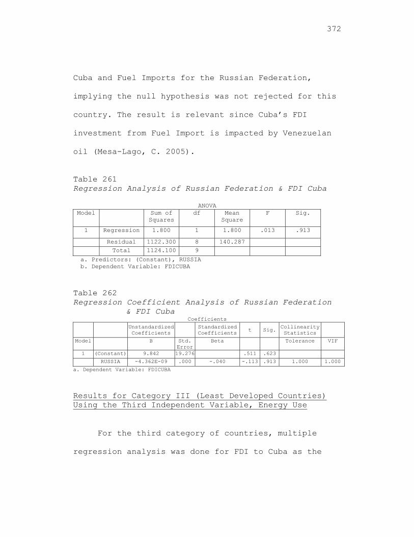
372

Cuba and Fuel Imports for the Russian Federation,

implying the null hypothesis was not rejected for this

country. The result is relevant since Cuba’s FDI

investment from Fuel Import is impacted by Venezuelan

oil (Mesa-Lago, C. 2005).

Table 261 Regression Analysis of Russian Federation & FDI Cuba

ANOVA Model Sum of

Squares df Mean

Square F Sig.

1 Regression 1.800 1 1.800 .013 .913

Residual 1122.300 8 140.287 Total 1124.100 9

a. Predictors: (Constant), RUSSIA b. Dependent Variable: FDICUBA

Table 262 Regression Coefficient Analysis of Russian Federation

& FDI Cuba Coefficients

Unstandardized Coefficients

Standardized Coefficients t Sig.

Collinearity Statistics

Model B Std. Error

Beta Tolerance VIF

1 (Constant) 9.842 19.276 .511 .623

RUSSIA -4.362E-09 .000 -.040 -.113 .913 1.000 1.000

a. Dependent Variable: FDICUBA

Results for Category III (Least Developed Countries) Using the Third Independent Variable, Energy Use

For the third category of countries, multiple

regression analysis was done for FDI to Cuba as the

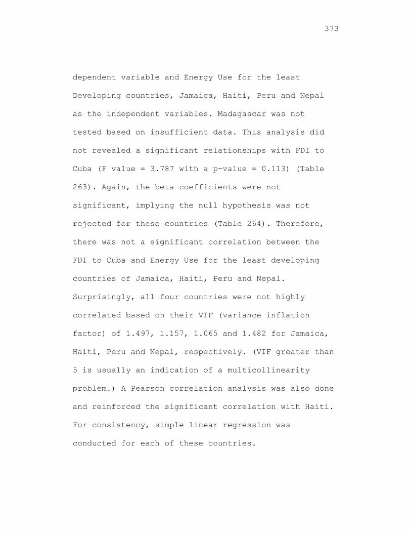
373

dependent variable and Energy Use for the least

Developing countries, Jamaica, Haiti, Peru and Nepal

as the independent variables. Madagascar was not

tested based on insufficient data. This analysis did

not revealed a significant relationships with FDI to

Cuba (F value = 3.787 with a p-value = 0.113) (Table

263). Again, the beta coefficients were not

significant, implying the null hypothesis was not

rejected for these countries (Table 264). Therefore,

there was not a significant correlation between the

FDI to Cuba and Energy Use for the least developing

countries of Jamaica, Haiti, Peru and Nepal.

Surprisingly, all four countries were not highly

correlated based on their VIF (variance inflation

factor) of 1.497, 1.157, 1.065 and 1.482 for Jamaica,

Haiti, Peru and Nepal, respectively. (VIF greater than

5 is usually an indication of a multicollinearity

problem.) A Pearson correlation analysis was also done

and reinforced the significant correlation with Haiti.

For consistency, simple linear regression was

conducted for each of these countries.

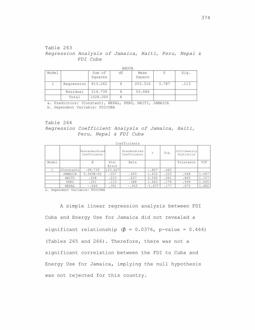
374

Table 263 Regression Analysis of Jamaica, Haiti, Peru, Nepal &

FDI Cuba

ANOVA Model Sum of

Squares df Mean

Square F Sig.

1 Regression 813.262 4 203.316 3.787 .113

Residual 214.738 4 53.684 Total 1028.000 8

a. Predictors: (Constant), NEPAL, PERU, HAITI, JAMAICA b. Dependent Variable: FDICUBA Table 264 Regression Coefficient Analysis of Jamaica, Haiti,

Peru, Nepal & FDI Cuba

Coefficients

Unstandardized Coefficients Standardized

Coefficients t Sig. Collinearity Statistics

Model B Std. Error

Beta Tolerance VIF

1 (Constant) -99.735 123.607 -.807 .465 JAMAICA 5.363E-02 .037 .400 1.432 .225 .668 1.497 HAITI .558 .215 .637 2.592 .061 .865 1.157 PERU .201 .123 .388 1.643 .176 .939 1.065 NEPAL -.640 .391 -.455 -1.637 .177 .675 1.482

a. Dependent Variable: FDICUBA

A simple linear regression analysis between FDI

Cuba and Energy Use for Jamaica did not revealed a

significant relationship ( = 0.0376, p-value = 0.464)

(Tables 265 and 266). Therefore, there was not a

significant correlation between the FDI to Cuba and

Energy Use for Jamaica, implying the null hypothesis

was not rejected for this country.

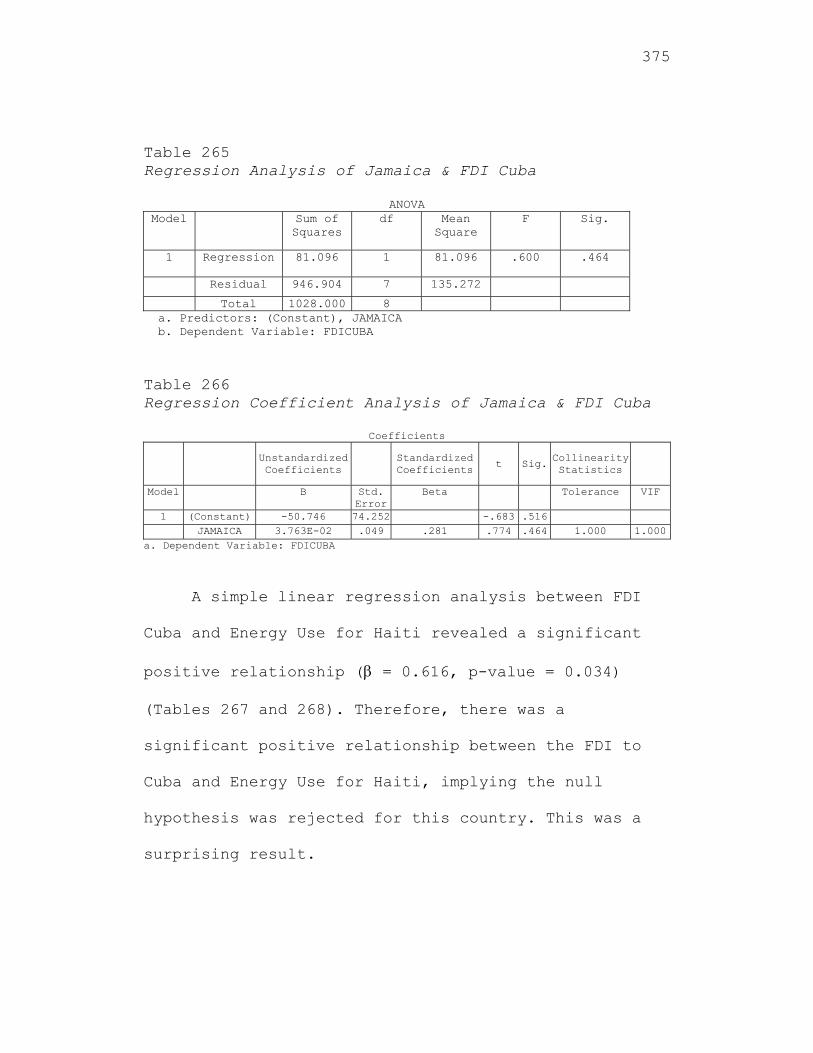
375

Table 265 Regression Analysis of Jamaica & FDI Cuba

ANOVA Model Sum of

Squares df Mean

Square F Sig.

1 Regression 81.096 1 81.096 .600 .464

Residual 946.904 7 135.272

Total 1028.000 8 a. Predictors: (Constant), JAMAICA b. Dependent Variable: FDICUBA

Table 266 Regression Coefficient Analysis of Jamaica & FDI Cuba

Coefficients

Unstandardized Coefficients

Standardized Coefficients t Sig.

Collinearity Statistics

Model B Std. Error

Beta Tolerance VIF

1 (Constant) -50.746 74.252 -.683 .516 JAMAICA 3.763E-02 .049 .281 .774 .464 1.000 1.000

a. Dependent Variable: FDICUBA

A simple linear regression analysis between FDI

Cuba and Energy Use for Haiti revealed a significant

positive relationship ( = 0.616, p-value = 0.034)

(Tables 267 and 268). Therefore, there was a

significant positive relationship between the FDI to

Cuba and Energy Use for Haiti, implying the null

hypothesis was rejected for this country. This was a

surprising result.

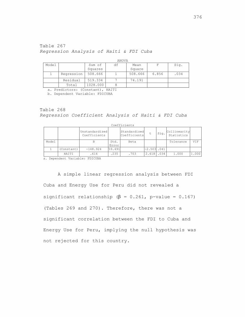
376

Table 267 Regression Analysis of Haiti & FDI Cuba

ANOVA Model Sum of

Squares df Mean

Square F Sig.

1 Regression 508.666 1 508.666 6.856 .034

Residual 519.334 7 74.191 Total 1028.000 8

a. Predictors: (Constant), HAITI b. Dependent Variable: FDICUBA

Table 268 Regression Coefficient Analysis of Haiti & FDI Cuba

Coefficients

Unstandardized Coefficients

Standardized Coefficients

t Sig. Collinearity Statistics

Model B Std. Error

Beta Tolerance VIF

1 (Constant) -148.924 59.491 -2.503 .041

HAITI .616 .235 .703 2.618 .034 1.000 1.000

a. Dependent Variable: FDICUBA

A simple linear regression analysis between FDI

Cuba and Energy Use for Peru did not revealed a

significant relationship ( = 0.261, p-value = 0.167)

(Tables 269 and 270). Therefore, there was not a

significant correlation between the FDI to Cuba and

Energy Use for Peru, implying the null hypothesis was

not rejected for this country.

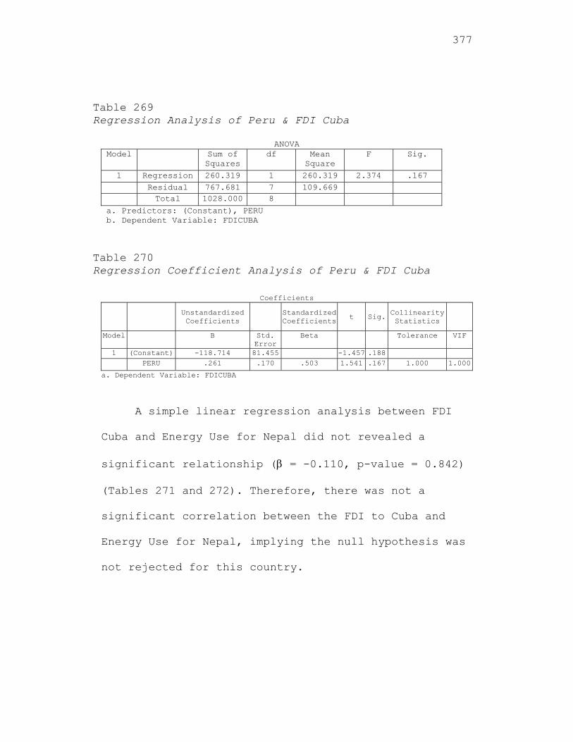
377

Table 269 Regression Analysis of Peru & FDI Cuba

ANOVA Model Sum of

Squares df Mean

Square F Sig.

1 Regression 260.319 1 260.319 2.374 .167 Residual 767.681 7 109.669 Total 1028.000 8

a. Predictors: (Constant), PERU b. Dependent Variable: FDICUBA

Table 270 Regression Coefficient Analysis of Peru & FDI Cuba

Coefficients

Unstandardized Coefficients

Standardized Coefficients

t Sig. Collinearity Statistics

Model B Std. Error

Beta Tolerance VIF

1 (Constant) -118.714 81.455 -1.457 .188 PERU .261 .170 .503 1.541 .167 1.000 1.000

a. Dependent Variable: FDICUBA

A simple linear regression analysis between FDI

Cuba and Energy Use for Nepal did not revealed a

significant relationship ( = -0.110, p-value = 0.842)

(Tables 271 and 272). Therefore, there was not a

significant correlation between the FDI to Cuba and

Energy Use for Nepal, implying the null hypothesis was

not rejected for this country.

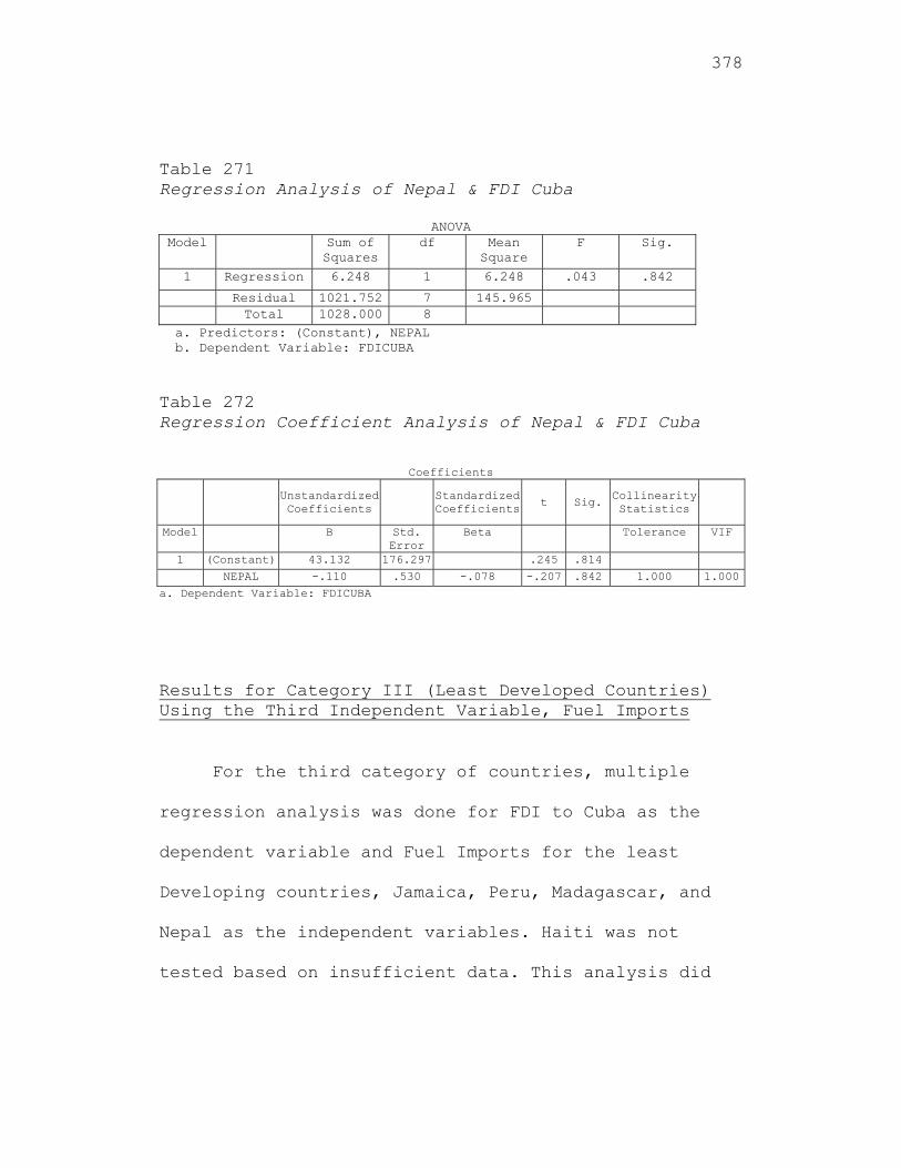
378

Table 271 Regression Analysis of Nepal & FDI Cuba

ANOVA Model Sum of

Squares df Mean

Square F Sig.

1 Regression 6.248 1 6.248 .043 .842

Residual 1021.752 7 145.965 Total 1028.000 8

a. Predictors: (Constant), NEPAL b. Dependent Variable: FDICUBA Table 272 Regression Coefficient Analysis of Nepal & FDI Cuba

Coefficients

Unstandardized Coefficients

Standardized Coefficients t Sig.

Collinearity Statistics

Model B Std. Error

Beta Tolerance VIF

1 (Constant) 43.132 176.297 .245 .814

NEPAL -.110 .530 -.078 -.207 .842 1.000 1.000

a. Dependent Variable: FDICUBA

Results for Category III (Least Developed Countries) Using the Third Independent Variable, Fuel Imports

For the third category of countries, multiple

regression analysis was done for FDI to Cuba as the

dependent variable and Fuel Imports for the least

Developing countries, Jamaica, Peru, Madagascar, and

Nepal as the independent variables. Haiti was not

tested based on insufficient data. This analysis did

379

not revealed any significant relationships with FDI to

Cuba (F value = 2.794 with a p-value = 0.145) (Table

273). Again, the beta coefficients were not

significant, implying the null hypothesis was not

rejected for these countries (Table 274). Therefore,

there was not a significant correlation between the

FDI to Cuba and Fuel Imports for the least developing

countries of Jamaica, Peru, Madagascar, and Nepal.

Like above, Fuel Imports for two of the four countries

were not highly correlated with VIFs (variance

inflation factor) of 8.708, 15.880, 4.558, and 1.183

for Jamaica, Peru, Madagascar and Nepal, respectively.

(VIF greater than 5 is usually an indication of a

multicollinearity problem.) A correlation analysis was

also done and reinforced with the low and high

correlation among these variables. Simple linear

regression was conducted for each of these countries.

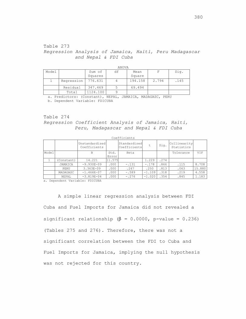
380

Table 273 Regression Analysis of Jamaica, Haiti, Peru Madagascar

and Nepal & FDI Cuba

ANOVA Model Sum of

Squares df Mean

Square F Sig.

1 Regression 776.631 4 194.158 2.794 .145

Residual 347.469 5 69.494 Total 1124.100 9

a. Predictors: (Constant), NEPAL, JAMAICA, MADAGASC, PERU b. Dependent Variable: FDICUBA

Table 274 Regression Coefficient Analysis of Jamaica, Haiti,

Peru, Madagascar and Nepal & FDI Cuba

Coefficients Unstandardized

Coefficients Standardized Coefficients t Sig.

Collinearity Statistics

Model B Std. Error

Beta Tolerance VIF

1 (Constant) 14.221 11.575 1.229 .274 JAMAICA -9.930E-09 .000 -.131 -.178 .866 .115 8.708 PERU 3.363E-09 .000 .247 .250 .813 .063 15.880 MADAGASC -1.466E-07 .000 -.589 -1.109 .318 .219 4.558 NEPAL -3.819E-04 .000 -.276 -1.020 .354 .845 1.183

a. Dependent Variable: FDICUBA

A simple linear regression analysis between FDI

Cuba and Fuel Imports for Jamaica did not revealed a

significant relationship ( = 0.0000, p-value = 0.236)

(Tables 275 and 276). Therefore, there was not a

significant correlation between the FDI to Cuba and

Fuel Imports for Jamaica, implying the null hypothesis

was not rejected for this country.

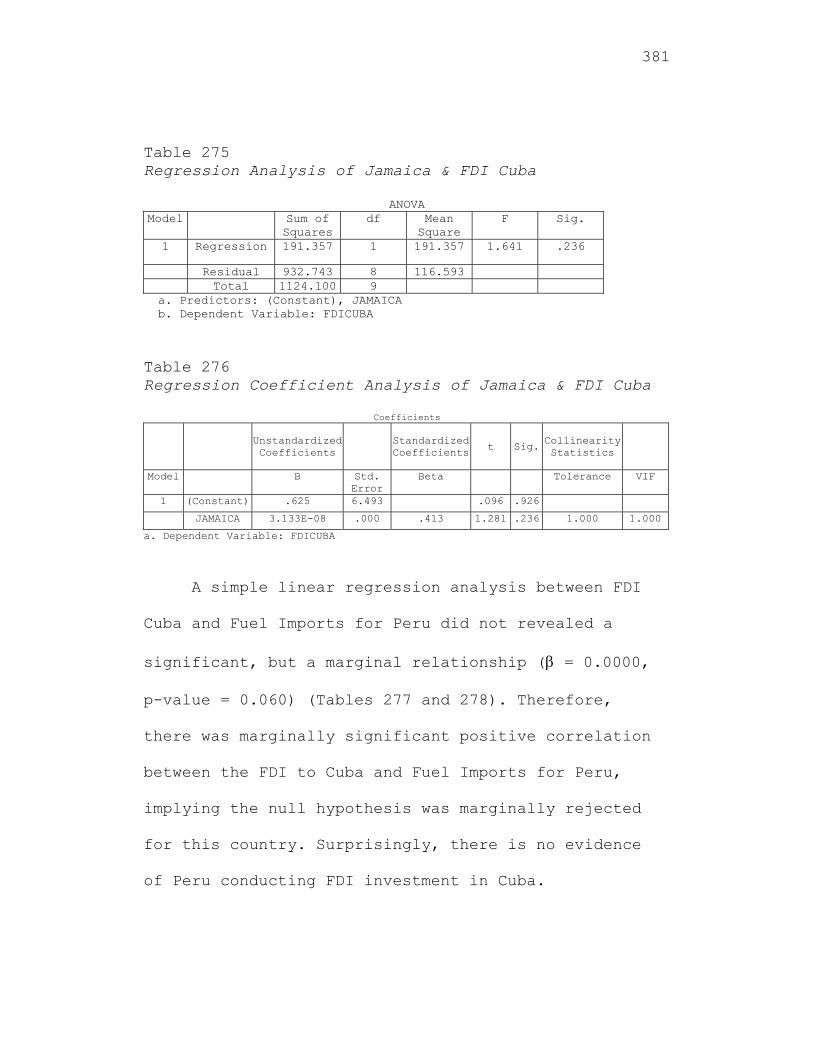
381

Table 275 Regression Analysis of Jamaica & FDI Cuba

ANOVA Model Sum of

Squares df Mean

Square F Sig.

1 Regression 191.357 1 191.357 1.641 .236

Residual 932.743 8 116.593 Total 1124.100 9

a. Predictors: (Constant), JAMAICA b. Dependent Variable: FDICUBA

Table 276 Regression Coefficient Analysis of Jamaica & FDI Cuba

Coefficients

Unstandardized Coefficients

Standardized Coefficients t Sig.

Collinearity Statistics

Model B Std. Error

Beta Tolerance VIF

1 (Constant) .625 6.493 .096 .926

JAMAICA 3.133E-08 .000 .413 1.281 .236 1.000 1.000

a. Dependent Variable: FDICUBA

A simple linear regression analysis between FDI

Cuba and Fuel Imports for Peru did not revealed a

significant, but a marginal relationship ( = 0.0000,

p-value = 0.060) (Tables 277 and 278). Therefore,

there was marginally significant positive correlation

between the FDI to Cuba and Fuel Imports for Peru,

implying the null hypothesis was marginally rejected

for this country. Surprisingly, there is no evidence

of Peru conducting FDI investment in Cuba.

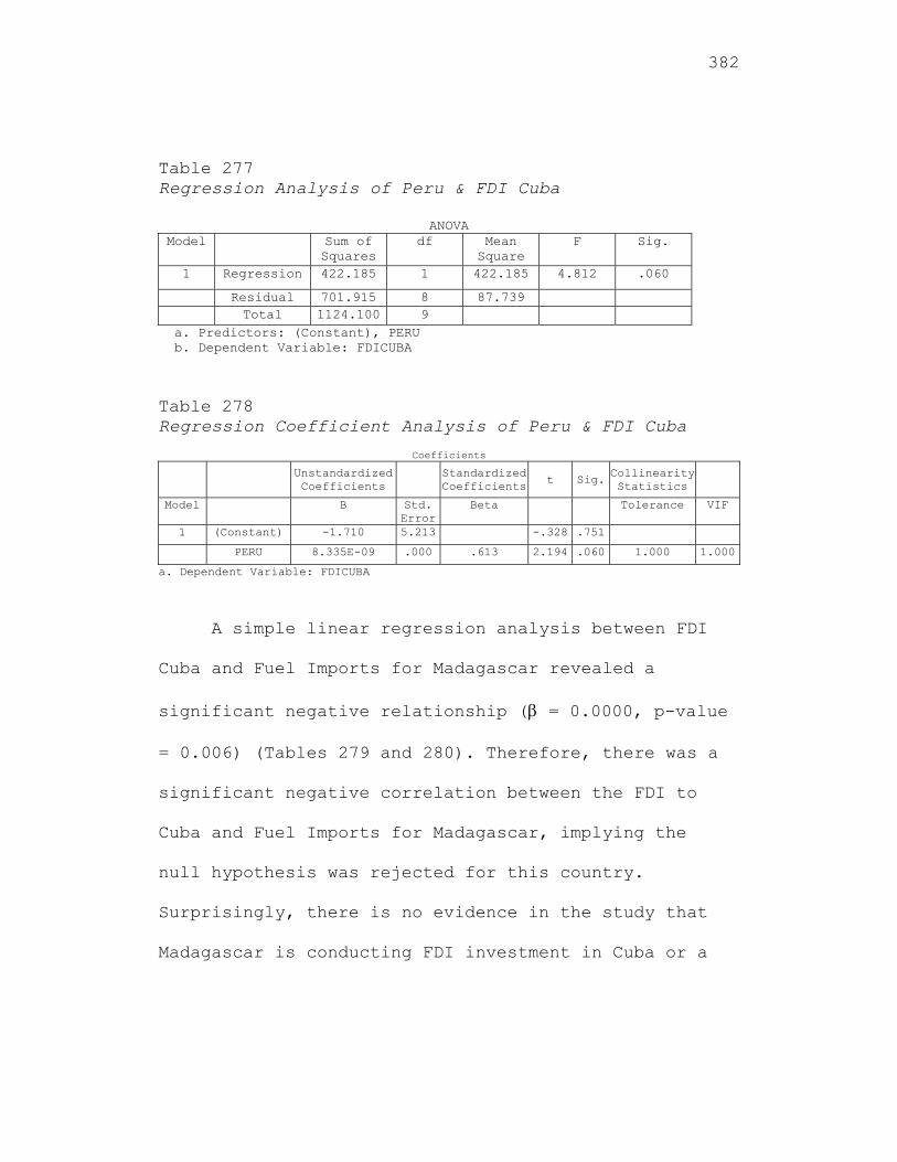
382

Table 277 Regression Analysis of Peru & FDI Cuba

ANOVA Model Sum of

Squares df Mean

Square F Sig.

1 Regression 422.185 1 422.185 4.812 .060

Residual 701.915 8 87.739 Total 1124.100 9

a. Predictors: (Constant), PERU b. Dependent Variable: FDICUBA

Table 278 Regression Coefficient Analysis of Peru & FDI Cuba

Coefficients Unstandardized

Coefficients

Standardized Coefficients

t Sig.Collinearity Statistics

Model B Std. Error

Beta Tolerance VIF

1 (Constant) -1.710 5.213 -.328 .751

PERU 8.335E-09 .000 .613 2.194 .060 1.000 1.000

a. Dependent Variable: FDICUBA

A simple linear regression analysis between FDI

Cuba and Fuel Imports for Madagascar revealed a

significant negative relationship ( = 0.0000, p-value

= 0.006) (Tables 279 and 280). Therefore, there was a

significant negative correlation between the FDI to

Cuba and Fuel Imports for Madagascar, implying the

null hypothesis was rejected for this country.

Surprisingly, there is no evidence in the study that

Madagascar is conducting FDI investment in Cuba or a

383

correlation between Madagascar’s Fuel Import and FDI

to Cuba.

Table 279 Regression Analysis of Madagascar & FDI Cuba

ANOVA Model Sum of

Squares df Mean

Square F Sig.

1 Regression 703.634 1 703.634 13.388 .006

Residual 420.466 8 52.558

Total 1124.100 9

a. Predictors: (Constant), MADAGASC b. Dependent Variable: FDICUBA

Table 280 Regression Coefficient Analysis of Madagascar & FDI

Cuba

Coefficients

Unstandardized Coefficients

Standardized Coefficients t Sig.

Collinearity Statistics

Model B Std. Error

Beta Tolerance VIF

1 (Constant) 17.180 3.460 4.966 .001

MADAGASC -1.970E-07 .000 -.791 -3.659 .006 1.000 1.000

a. Dependent Variable: FDICUBA

A simple linear regression analysis between FDI

Cuba and Fuel Imports for Nepal did not revealed a

significant relationship ( = -0.00064, p-value =

0.179) (Tables 281 and 282). Therefore, there was not

a significant correlation between the FDI to Cuba and

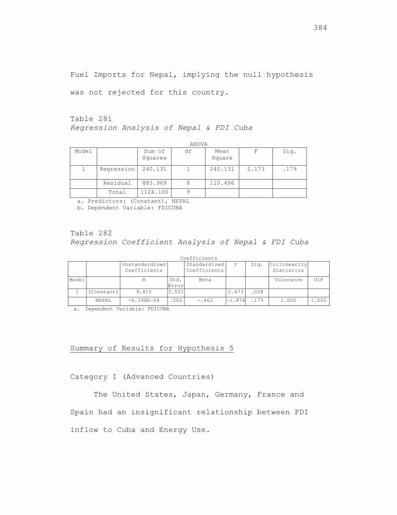
384

Fuel Imports for Nepal, implying the null hypothesis

was not rejected for this country.

Table 281 Regression Analysis of Nepal & FDI Cuba

ANOVA Model Sum of

Squares df Mean

Square F Sig.

1 Regression 240.131 1 240.131 2.173 .179

Residual 883.969 8 110.496

Total 1124.100 9

a. Predictors: (Constant), NEPAL b. Dependent Variable: FDICUBA

Table 282 Regression Coefficient Analysis of Nepal & FDI Cuba

Coefficients Unstandardized

Coefficients Standardized

Coefficientst Sig. Collinearity

Statistics

Model B Std. Error

Beta Tolerance VIF

1 (Constant) 9.410 3.521 2.673 .028

NEPAL -6.398E-04 .000 -.462 -1.474 .179 1.000 1.000

a. Dependent Variable: FDICUBA

Summary of Results for Hypothesis 5

Category I (Advanced Countries)

The United States, Japan, Germany, France and

Spain had an insignificant relationship between FDI

inflow to Cuba and Energy Use.

385

The United States, Japan, Germany, France and

Spain had an insignificant relationship between FDI

inflow to Cuba and Fuel Imports.

Category II (Developing Countries)

China, India and the Russian Federation had an

insignificant relationship between FDI inflow to Cuba

and Energy Use.

Multiple regression results are not appropriate

when there are multicollinearity problems. China,

India and the Russian Federation had an insignificant

relationship between FDI inflow to Cuba and Fuel

Imports.

Category III (Least Developing Countries)

Significant positive relationship existed between

FDI inflow to Cuba and Energy Use for Haiti.

Insignificant results were found for Jamaica, Peru and

Nepal, while Madagascar was not tested based on

insufficient data.

386

Jamaica and Nepal had an insignificant

relationship between FDI inflow to Cuba and Fuel

Imports, while Peru showed a positive marginal result.

Madagascar revealed a significant negative

relationship and Haiti was not tested based on

insufficient data.

Results for Hypothesis 6

FDI to Cuba was the dependent variable. For the

advanced countries, the independent variables were

Transportation and Communication for the United

States, Japan, Germany, France and Spain (Sawalha,

2007). The independent variables for the developing

countries were Transportation and Communication for

China, India and the Russian Federation (Sawalha,

2007). The independent variables for the Least

Developed Countries (LCD’s) were Transportation and

Communication for Jamaica, Haiti, Peru, Madagascar and

Nepal. The Republic of Cuba’s Transportation and

Communication was not included in the model as there

were only three data points. The Transportation and

387

Communication hypothesis included three variables, Air

Transport (as measured in passenger carried), Fixed

Line and Mobile Phone Subscribers (as measured per 100

of the population) and Internet Users (as measured per

100 of the population).

The sixth hypothesis to be tested is:

Hypothesis H06: The level of contribution of FDI

inflow to Cuba is not significantly related to

the Transportation and Communication for the

three groups of countries.

Hypothesis HA6: The level of contribution of FDI

inflow to Cuba is significantly related to the

Transportation and Communication for the three

groups of countries.

The multiple regression models to test Hypothesis 6

are listed below.

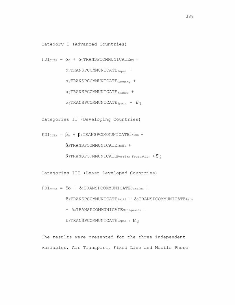
388

Category I (Advanced Countries)

FDICUBA = αO + α1TRANSPCOMMUNICATEUS +

α2TRANSPCOMMUNICATEJapan +

α3TRANSPCOMMUNICATEGermany +

α4TRANSPCOMMUNICATEFrance +

α5TRANSPCOMMUNICATESpain + ε1

Categories II (Developing Countries)

FDICUBA = O + 1TRANSPCOMMUNICATEChina +

2TRANSPCOMMUNICATEIndia +

3TRANSPCOMMUNICATERussian Federation +ε2

Categories III (Least Developed Countries)

FDICUBA = δ + δ1TRANSPCOMMUNICATEJamaica +

δ2TRANSPCOMMUNICATEHaiti + δ3TRANSPCOMMUNICATEPeru

+ δ4TRANSPCOMMUNICATEMadagascar +

δ5TRANSPCOMMUNICATENepal + ε3

The results were presented for the three independent

variables, Air Transport, Fixed Line and Mobile Phone

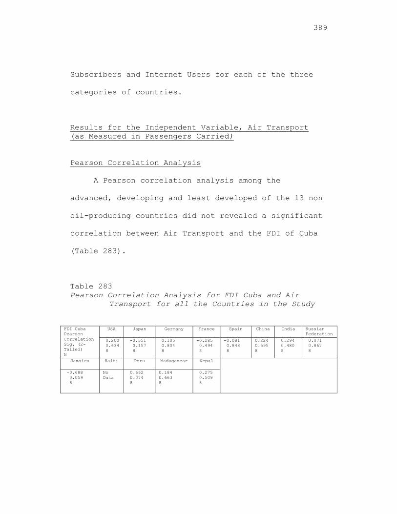
389

Subscribers and Internet Users for each of the three

categories of countries.

Results for the Independent Variable, Air Transport (as Measured in Passengers Carried)

Pearson Correlation Analysis

A Pearson correlation analysis among the

advanced, developing and least developed of the 13 non

oil-producing countries did not revealed a significant

correlation between Air Transport and the FDI of Cuba

(Table 283).

Table 283 Pearson Correlation Analysis for FDI Cuba and Air

Transport for all the Countries in the Study

FDI Cuba Pearson Correlation Sig. (2-Tailed) N

USA Japan Germany France Spain China India Russian Federation

0.200 0.634 8

-0.551 0.157 8

0.105 0.804 8

-0.285 0.494 8

-0.081 0.848 8

0.224 0.595 8

0.294 0.480 8

0.071 0.867 8

Jamaica Haiti Peru Madagascar Nepal

-0.688 0.059 8

No Data

0.662 0.074 8

0.184 0.663 8

0.275 0.509 8

390

Results for Category I (Advanced Countries) Using the First Independent Variable, Air Transport

The multiple regression analysis, with FDI of

Cuba as the dependent variable and Air Transport for

the advanced countries, the United States, Japan,

Germany, France and Spain as the independent

variables, did not revealed a significant

relationships. From the ANOVA, the F-value = 0.285

with a p-value = 0.888 implying that the model was not

significant (Table 284). This was also seen from the

multiple regression analysis where the beta

coefficients were not significant, implying the null

hypothesis was not rejected for these countries (Table

285). Therefore, there was not a significant

correlation between the FDI of Cuba and Air Transport

for these advanced countries, the United States,

Japan, Germany, France and Spain. From the

collinearity diagnostics, the variance inflation

factor (VIF) was 10.466, 16.764, 19.202, 22.193 and

12.741 for the United States, Japan, Germany, France

and Spain, respectively. (VIF greater than 5 is

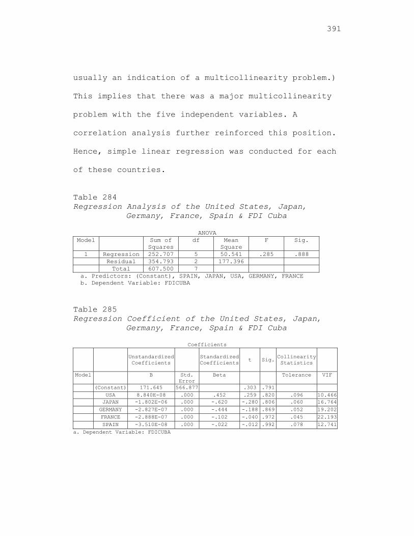
391

usually an indication of a multicollinearity problem.)

This implies that there was a major multicollinearity

problem with the five independent variables. A

correlation analysis further reinforced this position.

Hence, simple linear regression was conducted for each

of these countries.

Table 284 Regression Analysis of the United States, Japan,

Germany, France, Spain & FDI Cuba

ANOVA Model Sum of

Squares df Mean

Square F Sig.

1 Regression 252.707 5 50.541 .285 .888 Residual 354.793 2 177.396 Total 607.500 7

a. Predictors: (Constant), SPAIN, JAPAN, USA, GERMANY, FRANCE b. Dependent Variable: FDICUBA

Table 285 Regression Coefficient of the United States, Japan,

Germany, France, Spain & FDI Cuba

Coefficients

Unstandardized Coefficients

Standardized Coefficients

t Sig. Collinearity Statistics

Model B Std. Error

Beta Tolerance VIF

(Constant) 171.645 566.877 .303 .791 USA 8.840E-08 .000 .452 .259 .820 .096 10.466 JAPAN -1.802E-06 .000 -.620 -.280 .806 .060 16.764 GERMANY -2.827E-07 .000 -.444 -.188 .869 .052 19.202 FRANCE -2.888E-07 .000 -.102 -.040 .972 .045 22.193 SPAIN -3.510E-08 .000 -.022 -.012 .992 .078 12.741

a. Dependent Variable: FDICUBA

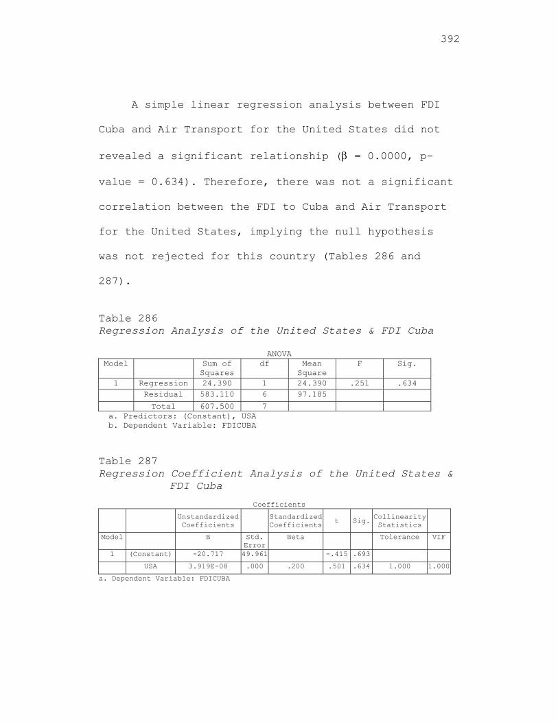
392

A simple linear regression analysis between FDI

Cuba and Air Transport for the United States did not

revealed a significant relationship ( = 0.0000, p-

value = 0.634). Therefore, there was not a significant

correlation between the FDI to Cuba and Air Transport

for the United States, implying the null hypothesis

was not rejected for this country (Tables 286 and

287).

Table 286 Regression Analysis of the United States & FDI Cuba

ANOVA Model Sum of

Squares df Mean

Square F Sig.

1 Regression 24.390 1 24.390 .251 .634 Residual 583.110 6 97.185

Total 607.500 7 a. Predictors: (Constant), USA b. Dependent Variable: FDICUBA

Table 287 Regression Coefficient Analysis of the United States &

FDI Cuba

Coefficients Unstandardized

Coefficients Standardized

Coefficientst Sig. Collinearity

Statistics

Model B Std. Error

Beta Tolerance VIF

1 (Constant) -20.717 49.961 -.415 .693

USA 3.919E-08 .000 .200 .501 .634 1.000 1.000

a. Dependent Variable: FDICUBA

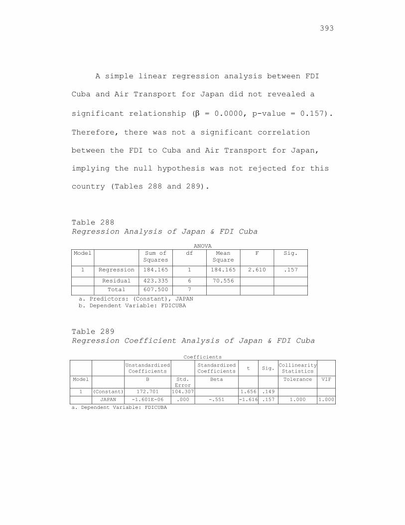
393

A simple linear regression analysis between FDI

Cuba and Air Transport for Japan did not revealed a

significant relationship ( = 0.0000, p-value = 0.157).

Therefore, there was not a significant correlation

between the FDI to Cuba and Air Transport for Japan,

implying the null hypothesis was not rejected for this

country (Tables 288 and 289).

Table 288 Regression Analysis of Japan & FDI Cuba

ANOVA

Model Sum of Squares

df Mean Square

F Sig.

1 Regression 184.165 1 184.165 2.610 .157

Residual 423.335 6 70.556

Total 607.500 7

a. Predictors: (Constant), JAPAN b. Dependent Variable: FDICUBA

Table 289 Regression Coefficient Analysis of Japan & FDI Cuba

Coefficients Unstandardized

Coefficients Standardized Coefficients t Sig.

Collinearity Statistics

Model B Std. Error

Beta Tolerance VIF

1 (Constant) 172.701 104.307 1.656 .149

JAPAN -1.601E-06 .000 -.551 -1.616 .157 1.000 1.000

a. Dependent Variable: FDICUBA

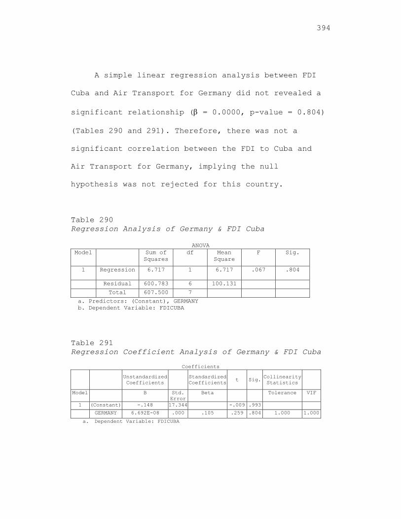
394

A simple linear regression analysis between FDI

Cuba and Air Transport for Germany did not revealed a

significant relationship ( = 0.0000, p-value = 0.804)

(Tables 290 and 291). Therefore, there was not a

significant correlation between the FDI to Cuba and

Air Transport for Germany, implying the null

hypothesis was not rejected for this country.

Table 290 Regression Analysis of Germany & FDI Cuba

ANOVA Model Sum of

Squares df Mean

Square F Sig.

1 Regression 6.717 1 6.717 .067 .804

Residual 600.783 6 100.131

Total 607.500 7

a. Predictors: (Constant), GERMANY b. Dependent Variable: FDICUBA

Table 291 Regression Coefficient Analysis of Germany & FDI Cuba

Coefficients

Unstandardized Coefficients

Standardized Coefficients

t Sig. Collinearity Statistics

Model B Std. Error

Beta Tolerance VIF

1 (Constant) -.148 17.344 -.009 .993

GERMANY 6.692E-08 .000 .105 .259 .804 1.000 1.000

a. Dependent Variable: FDICUBA

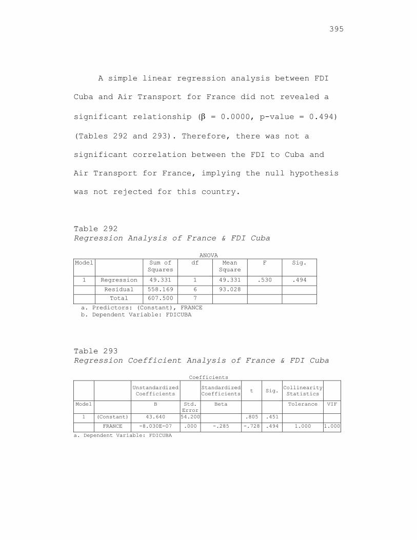
395

A simple linear regression analysis between FDI

Cuba and Air Transport for France did not revealed a

significant relationship ( = 0.0000, p-value = 0.494)

(Tables 292 and 293). Therefore, there was not a

significant correlation between the FDI to Cuba and

Air Transport for France, implying the null hypothesis

was not rejected for this country.

Table 292 Regression Analysis of France & FDI Cuba

ANOVA Model Sum of

Squares df Mean

Square F Sig.

1 Regression 49.331 1 49.331 .530 .494

Residual 558.169 6 93.028

Total 607.500 7

a. Predictors: (Constant), FRANCE b. Dependent Variable: FDICUBA

Table 293 Regression Coefficient Analysis of France & FDI Cuba

Coefficients

Unstandardized Coefficients

Standardized Coefficients t Sig.

Collinearity Statistics

Model B Std. Error

Beta Tolerance VIF

1 (Constant) 43.640 54.200 .805 .451

FRANCE -8.030E-07 .000 -.285 -.728 .494 1.000 1.000

a. Dependent Variable: FDICUBA

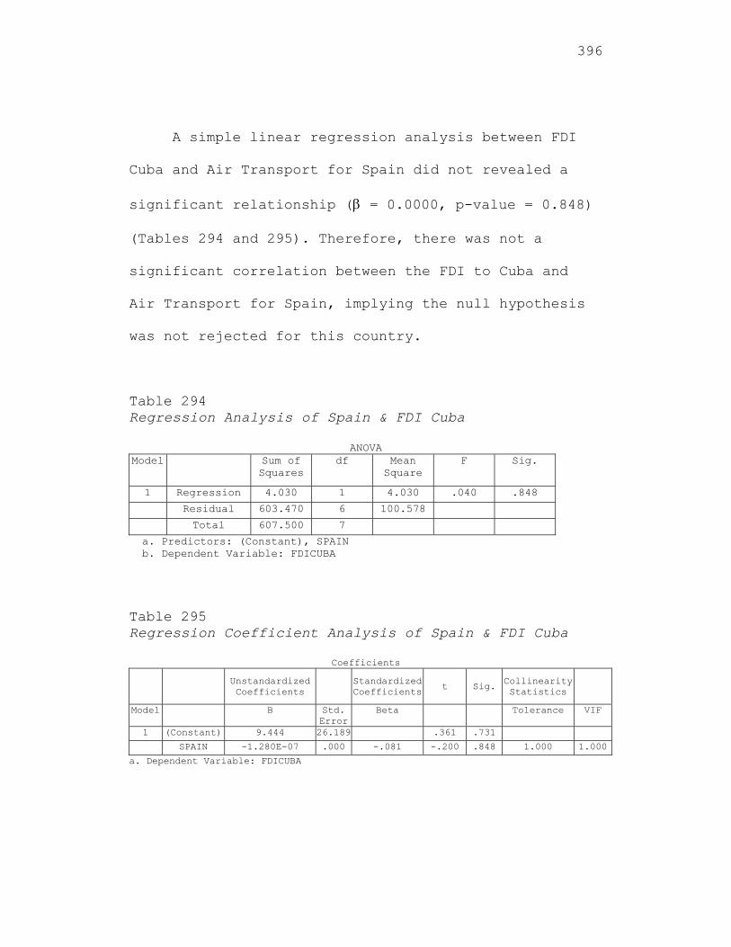
396

A simple linear regression analysis between FDI

Cuba and Air Transport for Spain did not revealed a

significant relationship ( = 0.0000, p-value = 0.848)

(Tables 294 and 295). Therefore, there was not a

significant correlation between the FDI to Cuba and

Air Transport for Spain, implying the null hypothesis

was not rejected for this country.

Table 294 Regression Analysis of Spain & FDI Cuba

ANOVA Model Sum of

Squares df Mean

Square F Sig.

1 Regression 4.030 1 4.030 .040 .848

Residual 603.470 6 100.578

Total 607.500 7

a. Predictors: (Constant), SPAIN b. Dependent Variable: FDICUBA

Table 295 Regression Coefficient Analysis of Spain & FDI Cuba

Coefficients

Unstandardized Coefficients

Standardized Coefficients

t Sig. Collinearity Statistics

Model B Std. Error

Beta Tolerance VIF

1 (Constant) 9.444 26.189 .361 .731

SPAIN -1.280E-07 .000 -.081 -.200 .848 1.000 1.000

a. Dependent Variable: FDICUBA

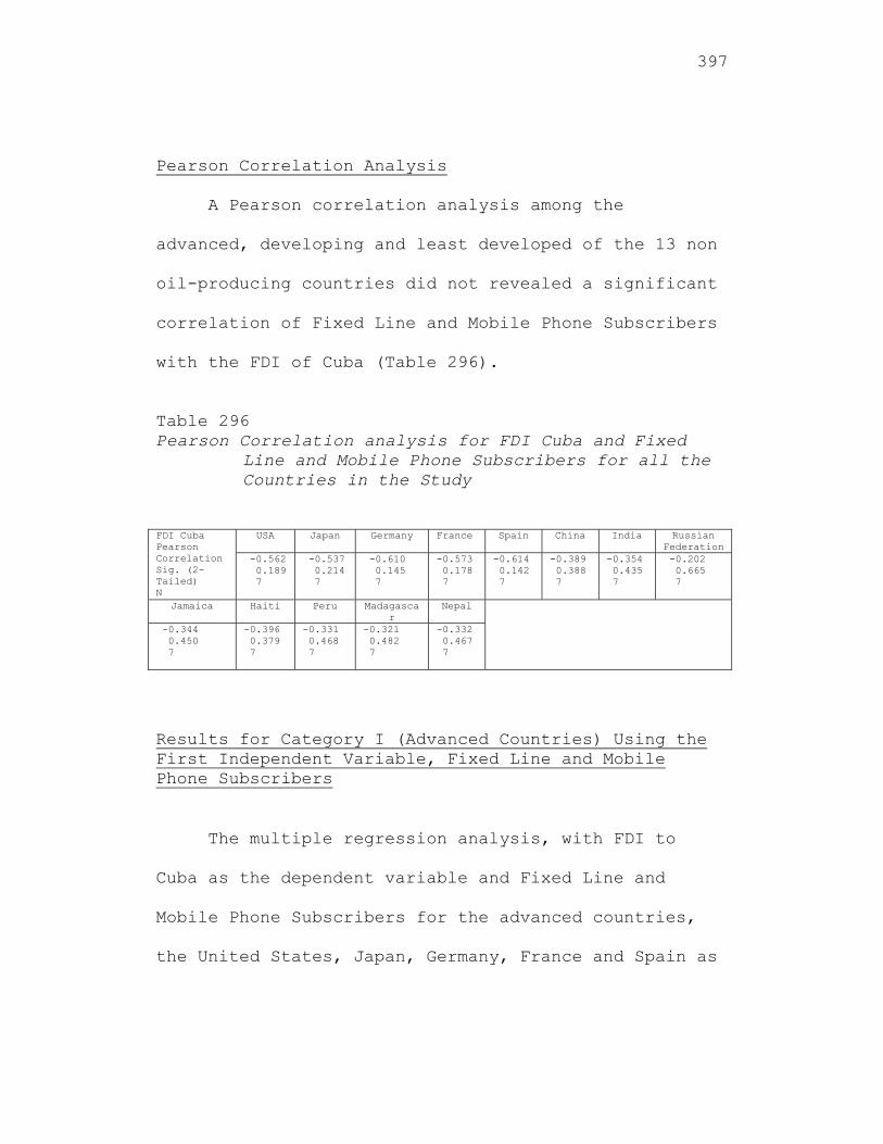
397

Pearson Correlation Analysis

A Pearson correlation analysis among the

advanced, developing and least developed of the 13 non

oil-producing countries did not revealed a significant

correlation of Fixed Line and Mobile Phone Subscribers

with the FDI of Cuba (Table 296).

Table 296 Pearson Correlation analysis for FDI Cuba and Fixed

Line and Mobile Phone Subscribers for all the Countries in the Study

FDI Cuba Pearson Correlation Sig. (2-Tailed) N

USA Japan Germany France Spain China India Russian Federation

-0.562 0.189 7

-0.537 0.214 7

-0.610 0.145 7

-0.573 0.178 7

-0.614 0.142 7

-0.389 0.388 7

-0.354 0.435 7

-0.202 0.665 7

Jamaica Haiti Peru Madagascar

Nepal

-0.344 0.450 7

-0.396 0.379 7

-0.331 0.468 7

-0.321 0.482 7

-0.332 0.467 7

Results for Category I (Advanced Countries) Using the First Independent Variable, Fixed Line and Mobile Phone Subscribers

The multiple regression analysis, with FDI to

Cuba as the dependent variable and Fixed Line and

Mobile Phone Subscribers for the advanced countries,

the United States, Japan, Germany, France and Spain as

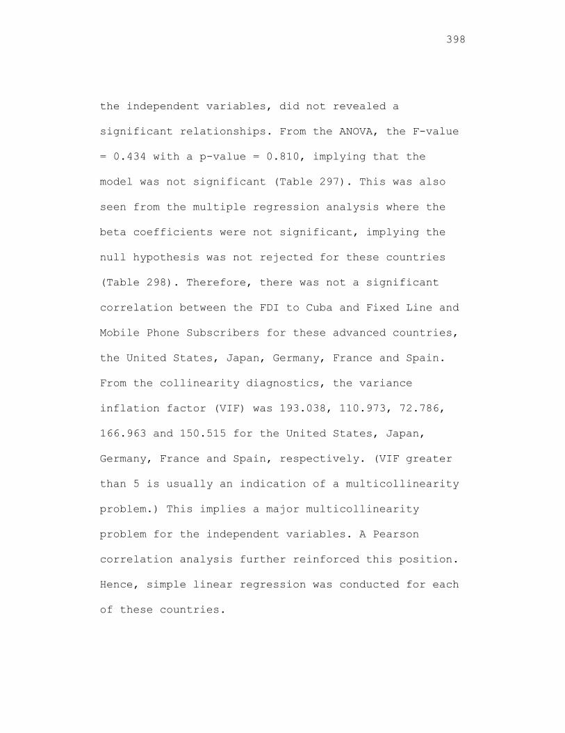
398

the independent variables, did not revealed a

significant relationships. From the ANOVA, the F-value

= 0.434 with a p-value = 0.810, implying that the

model was not significant (Table 297). This was also

seen from the multiple regression analysis where the

beta coefficients were not significant, implying the

null hypothesis was not rejected for these countries

(Table 298). Therefore, there was not a significant

correlation between the FDI to Cuba and Fixed Line and

Mobile Phone Subscribers for these advanced countries,

the United States, Japan, Germany, France and Spain.

From the collinearity diagnostics, the variance

inflation factor (VIF) was 193.038, 110.973, 72.786,

166.963 and 150.515 for the United States, Japan,

Germany, France and Spain, respectively. (VIF greater

than 5 is usually an indication of a multicollinearity

problem.) This implies a major multicollinearity

problem for the independent variables. A Pearson

correlation analysis further reinforced this position.

Hence, simple linear regression was conducted for each

of these countries.

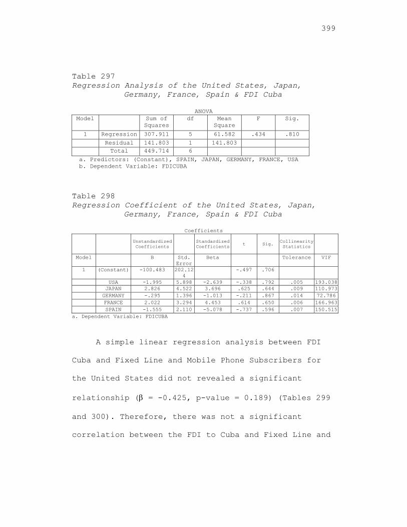
399

Table 297 Regression Analysis of the United States, Japan,

Germany, France, Spain & FDI Cuba

ANOVA Model Sum of

Squares df Mean

Square F Sig.

1 Regression 307.911 5 61.582 .434 .810

Residual 141.803 1 141.803 Total 449.714 6

a. Predictors: (Constant), SPAIN, JAPAN, GERMANY, FRANCE, USA b. Dependent Variable: FDICUBA Table 298 Regression Coefficient of the United States, Japan,

Germany, France, Spain & FDI Cuba

Coefficients

Unstandardized Coefficients Standardized

Coefficients t Sig. Collinearity Statistics

Model B Std. Error

Beta Tolerance VIF

1 (Constant) -100.483 202.124

-.497 .706

USA -1.995 5.898 -2.639 -.338 .792 .005 193.038 JAPAN 2.826 4.522 3.696 .625 .644 .009 110.973 GERMANY -.295 1.396 -1.013 -.211 .867 .014 72.786 FRANCE 2.022 3.294 4.453 .614 .650 .006 166.963 SPAIN -1.555 2.110 -5.078 -.737 .596 .007 150.515

a. Dependent Variable: FDICUBA

A simple linear regression analysis between FDI

Cuba and Fixed Line and Mobile Phone Subscribers for

the United States did not revealed a significant

relationship ( = -0.425, p-value = 0.189) (Tables 299

and 300). Therefore, there was not a significant

correlation between the FDI to Cuba and Fixed Line and

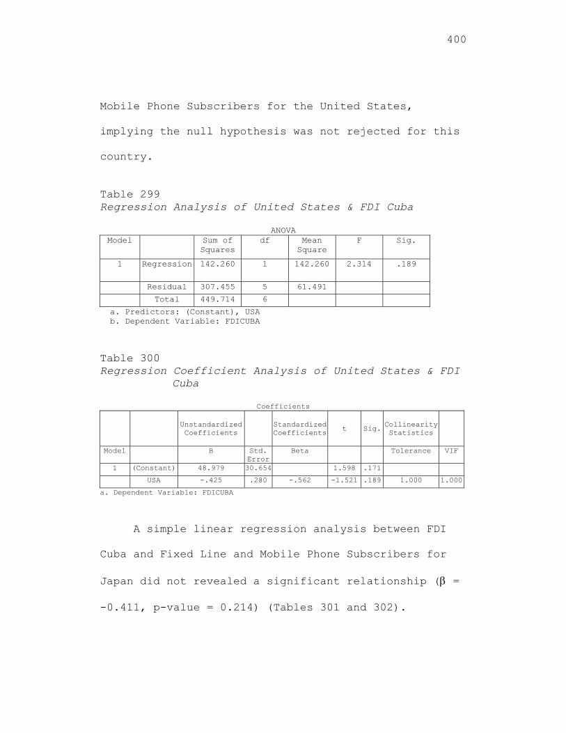
400

Mobile Phone Subscribers for the United States,

implying the null hypothesis was not rejected for this

country.

Table 299 Regression Analysis of United States & FDI Cuba

ANOVA Model Sum of

Squares df Mean

Square F Sig.

1 Regression 142.260 1 142.260 2.314 .189

Residual 307.455 5 61.491

Total 449.714 6

a. Predictors: (Constant), USA b. Dependent Variable: FDICUBA

Table 300 Regression Coefficient Analysis of United States & FDI

Cuba

Coefficients

Unstandardized Coefficients

Standardized Coefficients t Sig.

Collinearity Statistics

Model B Std. Error

Beta Tolerance VIF

1 (Constant) 48.979 30.654 1.598 .171

USA -.425 .280 -.562 -1.521 .189 1.000 1.000

a. Dependent Variable: FDICUBA

A simple linear regression analysis between FDI

Cuba and Fixed Line and Mobile Phone Subscribers for

Japan did not revealed a significant relationship ( =

-0.411, p-value = 0.214) (Tables 301 and 302).

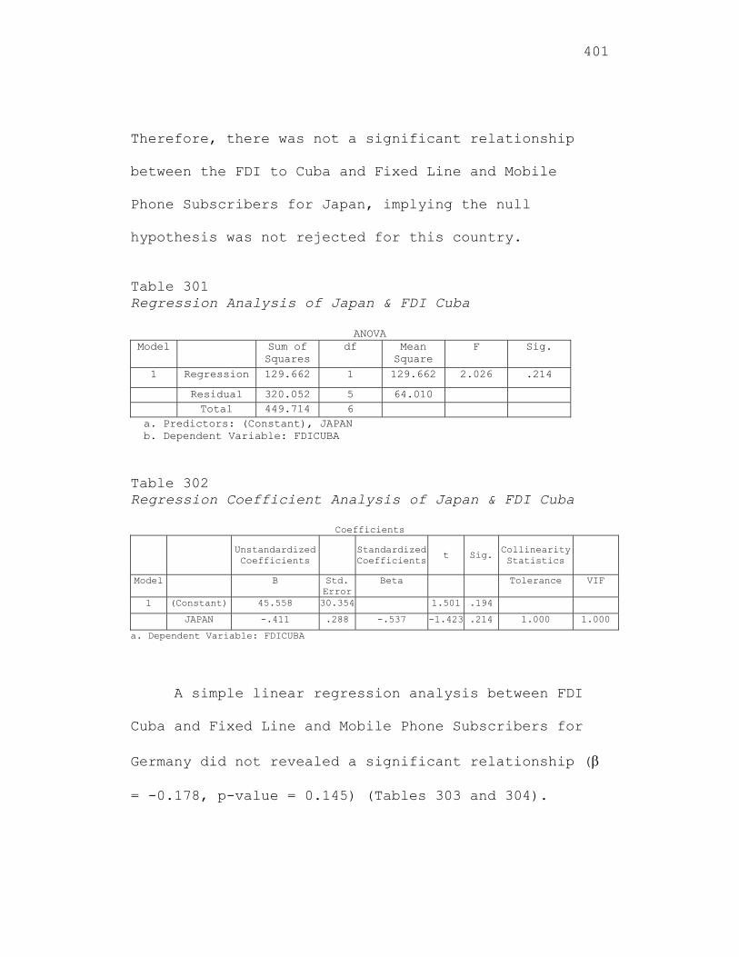
401

Therefore, there was not a significant relationship

between the FDI to Cuba and Fixed Line and Mobile

Phone Subscribers for Japan, implying the null

hypothesis was not rejected for this country.

Table 301 Regression Analysis of Japan & FDI Cuba

ANOVA Model Sum of

Squares df Mean

Square F Sig.

1 Regression 129.662 1 129.662 2.026 .214

Residual 320.052 5 64.010 Total 449.714 6

a. Predictors: (Constant), JAPAN b. Dependent Variable: FDICUBA

Table 302 Regression Coefficient Analysis of Japan & FDI Cuba

Coefficients

Unstandardized Coefficients

Standardized Coefficients

t Sig.Collinearity Statistics

Model B Std. Error

Beta Tolerance VIF

1 (Constant) 45.558 30.354 1.501 .194

JAPAN -.411 .288 -.537 -1.423 .214 1.000 1.000

a. Dependent Variable: FDICUBA

A simple linear regression analysis between FDI

Cuba and Fixed Line and Mobile Phone Subscribers for

Germany did not revealed a significant relationship (

= -0.178, p-value = 0.145) (Tables 303 and 304).

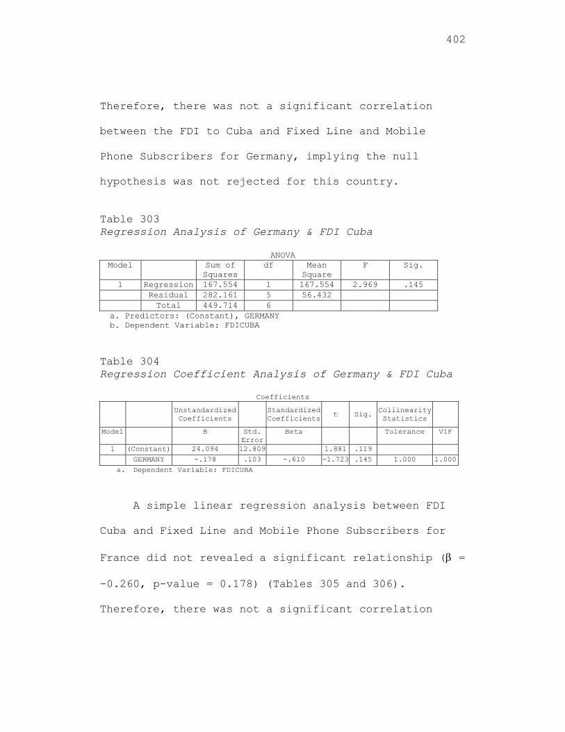
402

Therefore, there was not a significant correlation

between the FDI to Cuba and Fixed Line and Mobile

Phone Subscribers for Germany, implying the null

hypothesis was not rejected for this country.

Table 303 Regression Analysis of Germany & FDI Cuba

ANOVA Model Sum of

Squares df Mean

Square F Sig.

1 Regression 167.554 1 167.554 2.969 .145 Residual 282.161 5 56.432 Total 449.714 6

a. Predictors: (Constant), GERMANY b. Dependent Variable: FDICUBA

Table 304 Regression Coefficient Analysis of Germany & FDI Cuba

Coefficients

Unstandardized Coefficients

Standardized Coefficients

t Sig. Collinearity Statistics

Model B Std. Error

Beta Tolerance VIF

1 (Constant) 24.094 12.809 1.881 .119

GERMANY -.178 .103 -.610 -1.723 .145 1.000 1.000

a. Dependent Variable: FDICUBA

A simple linear regression analysis between FDI

Cuba and Fixed Line and Mobile Phone Subscribers for

France did not revealed a significant relationship ( =

-0.260, p-value = 0.178) (Tables 305 and 306).

Therefore, there was not a significant correlation

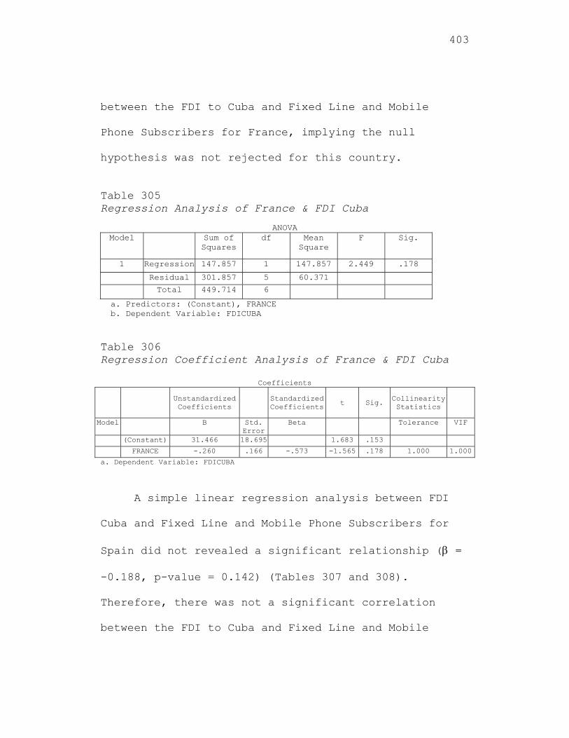
403

between the FDI to Cuba and Fixed Line and Mobile

Phone Subscribers for France, implying the null

hypothesis was not rejected for this country.

Table 305 Regression Analysis of France & FDI Cuba

ANOVA

Model Sum of Squares

df Mean Square

F Sig.

1 Regression 147.857 1 147.857 2.449 .178

Residual 301.857 5 60.371

Total 449.714 6

a. Predictors: (Constant), FRANCE b. Dependent Variable: FDICUBA

Table 306 Regression Coefficient Analysis of France & FDI Cuba

Coefficients

UnstandardizedCoefficients

Standardized Coefficients

t Sig. Collinearity Statistics

Model B Std. Error

Beta Tolerance VIF

(Constant) 31.466 18.695 1.683 .153

FRANCE -.260 .166 -.573 -1.565 .178 1.000 1.000

a. Dependent Variable: FDICUBA

A simple linear regression analysis between FDI

Cuba and Fixed Line and Mobile Phone Subscribers for

Spain did not revealed a significant relationship ( =

-0.188, p-value = 0.142) (Tables 307 and 308).

Therefore, there was not a significant correlation

between the FDI to Cuba and Fixed Line and Mobile

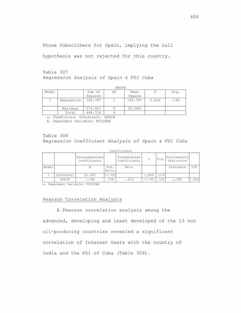
404

Phone Subscribers for Spain, implying the null

hypothesis was not rejected for this country.

Table 307 Regression Analysis of Spain & FDI Cuba

ANOVA Model Sum of

Squares df Mean

Square F Sig.

1 Regression 169.787 1 169.787 3.033 .142

Residual 279.927 5 55.985 Total 449.714 6

a. Predictors: (Constant), SPAIN b. Dependent Variable: FDICUBA Table 308 Regression Coefficient Analysis of Spain & FDI Cuba

Coefficients

Unstandardized Coefficients

Standardized Coefficients

t Sig.Collinearity Statistics

Model B Std. Error

Beta Tolerance VIF

1 (Constant) 22.387 11.725 1.909 .114 SPAIN -.188 .108 -.614 -1.741 .142 1.000 1.000

a. Dependent Variable: FDICUBA

Pearson Correlation Analysis

A Pearson correlation analysis among the

advanced, developing and least developed of the 13 non

oil-producing countries revealed a significant

correlation of Internet Users with the country of

India and the FDI of Cuba (Table 309).

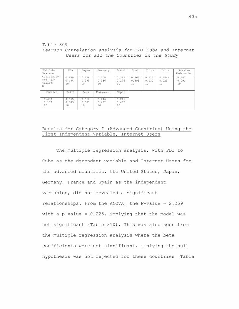
405

Table 309 Pearson Correlation analysis for FDI Cuba and Internet

Users for all the Countries in the Study FDI Cuba Pearson Correlation Sig. (2-Tailed) N

USA Japan Germany France Spain China India Russian Federation

0.280 0.434 10

0.368 0.295 10

0.308 0.386 10

0.382 0.276 10

0.363 0.303 10

0.512 0.130 10

0.684* 0.029 10

0.561 0.091 10

Jamaica Haiti Peru Madagascar Nepal

0.483 0.157 10

0.565 0.089 10

0.568 0.087 10

0.246 0.492 10

0.246 0.492 10

Results for Category I (Advanced Countries) Using the First Independent Variable, Internet Users

The multiple regression analysis, with FDI to

Cuba as the dependent variable and Internet Users for

the advanced countries, the United States, Japan,

Germany, France and Spain as the independent

variables, did not revealed a significant

relationships. From the ANOVA, the F-value = 2.259

with a p-value = 0.225, implying that the model was

not significant (Table 310). This was also seen from

the multiple regression analysis where the beta

coefficients were not significant, implying the null

hypothesis was not rejected for these countries (Table

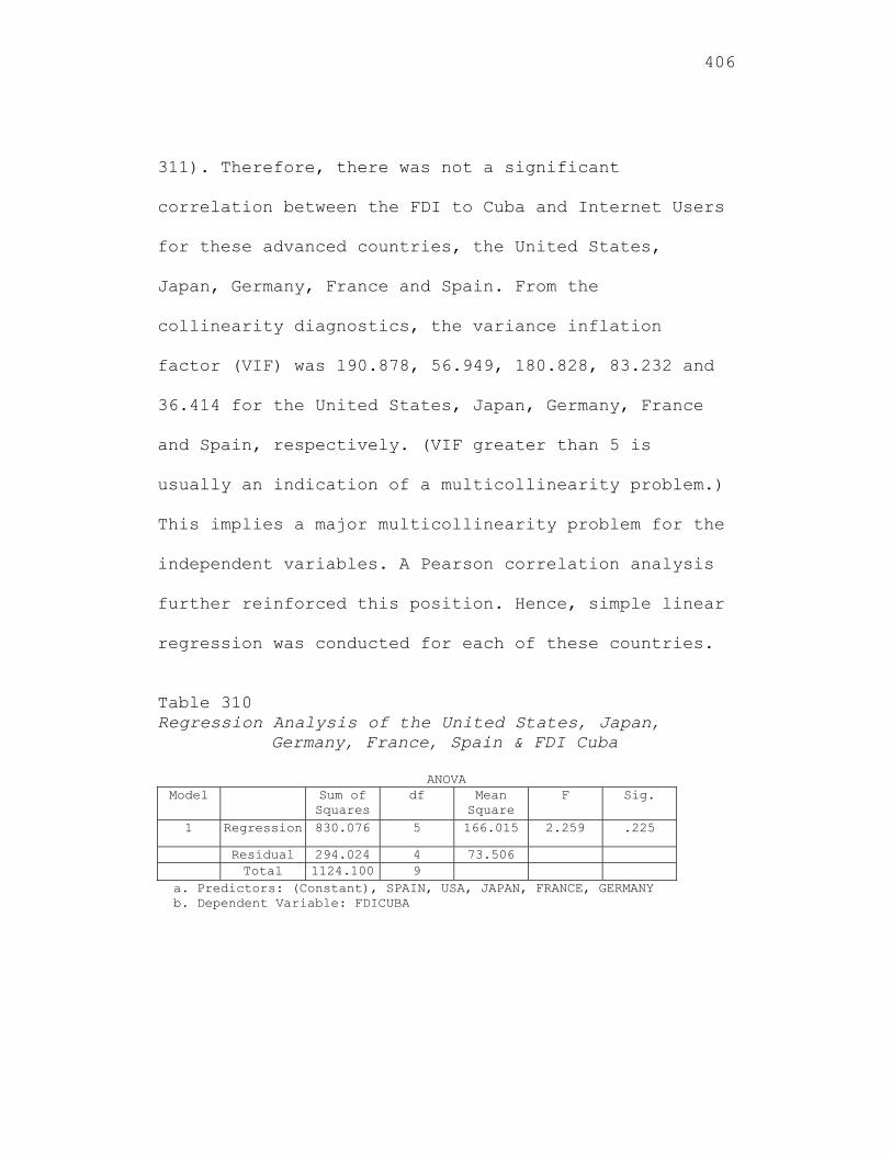
406

311). Therefore, there was not a significant

correlation between the FDI to Cuba and Internet Users

for these advanced countries, the United States,

Japan, Germany, France and Spain. From the

collinearity diagnostics, the variance inflation

factor (VIF) was 190.878, 56.949, 180.828, 83.232 and

36.414 for the United States, Japan, Germany, France

and Spain, respectively. (VIF greater than 5 is

usually an indication of a multicollinearity problem.)

This implies a major multicollinearity problem for the

independent variables. A Pearson correlation analysis

further reinforced this position. Hence, simple linear

regression was conducted for each of these countries.

Table 310 Regression Analysis of the United States, Japan,

Germany, France, Spain & FDI Cuba

ANOVA Model Sum of

Squares df Mean

Square F Sig.

1 Regression 830.076 5 166.015 2.259 .225

Residual 294.024 4 73.506 Total 1124.100 9

a. Predictors: (Constant), SPAIN, USA, JAPAN, FRANCE, GERMANY b. Dependent Variable: FDICUBA

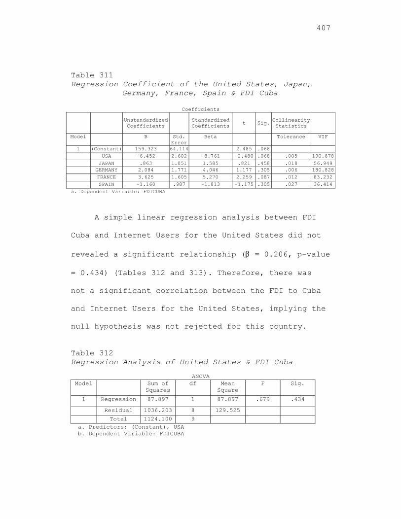
407

Table 311 Regression Coefficient of the United States, Japan,

Germany, France, Spain & FDI Cuba

Coefficients

Unstandardized Coefficients

Standardized Coefficients

t Sig. Collinearity Statistics

Model B Std. Error

Beta Tolerance VIF

1 (Constant) 159.323 64.114 2.485 .068 USA -6.452 2.602 -8.761 -2.480 .068 .005 190.878 JAPAN .863 1.051 1.585 .821 .458 .018 56.949 GERMANY 2.084 1.771 4.046 1.177 .305 .006 180.828 FRANCE 3.625 1.605 5.270 2.259 .087 .012 83.232 SPAIN -1.160 .987 -1.813 -1.175 .305 .027 36.414

a. Dependent Variable: FDICUBA

A simple linear regression analysis between FDI

Cuba and Internet Users for the United States did not

revealed a significant relationship ( = 0.206, p-value

= 0.434) (Tables 312 and 313). Therefore, there was

not a significant correlation between the FDI to Cuba

and Internet Users for the United States, implying the

null hypothesis was not rejected for this country.

Table 312 Regression Analysis of United States & FDI Cuba

ANOVA

Model Sum of Squares

df Mean Square

F Sig.

1 Regression 87.897 1 87.897 .679 .434

Residual 1036.203 8 129.525

Total 1124.100 9 a. Predictors: (Constant), USA b. Dependent Variable: FDICUBA

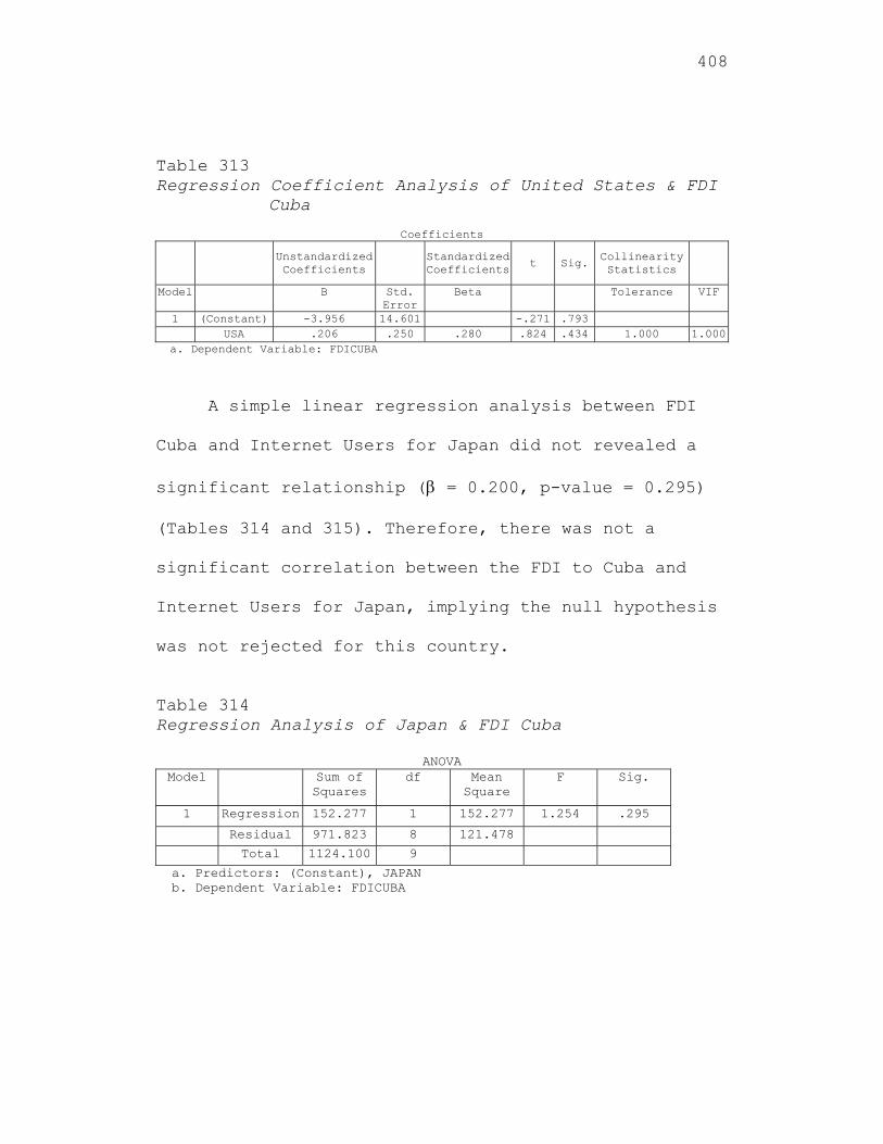
408

Table 313 Regression Coefficient Analysis of United States & FDI

Cuba

Coefficients

Unstandardized Coefficients

Standardized Coefficients t Sig.

Collinearity Statistics

Model B Std. Error

Beta Tolerance VIF

1 (Constant) -3.956 14.601 -.271 .793 USA .206 .250 .280 .824 .434 1.000 1.000

a. Dependent Variable: FDICUBA

A simple linear regression analysis between FDI

Cuba and Internet Users for Japan did not revealed a

significant relationship ( = 0.200, p-value = 0.295)

(Tables 314 and 315). Therefore, there was not a

significant correlation between the FDI to Cuba and

Internet Users for Japan, implying the null hypothesis

was not rejected for this country.

Table 314 Regression Analysis of Japan & FDI Cuba

ANOVA Model Sum of

Squares df Mean

Square F Sig.

1 Regression 152.277 1 152.277 1.254 .295

Residual 971.823 8 121.478

Total 1124.100 9

a. Predictors: (Constant), JAPAN b. Dependent Variable: FDICUBA

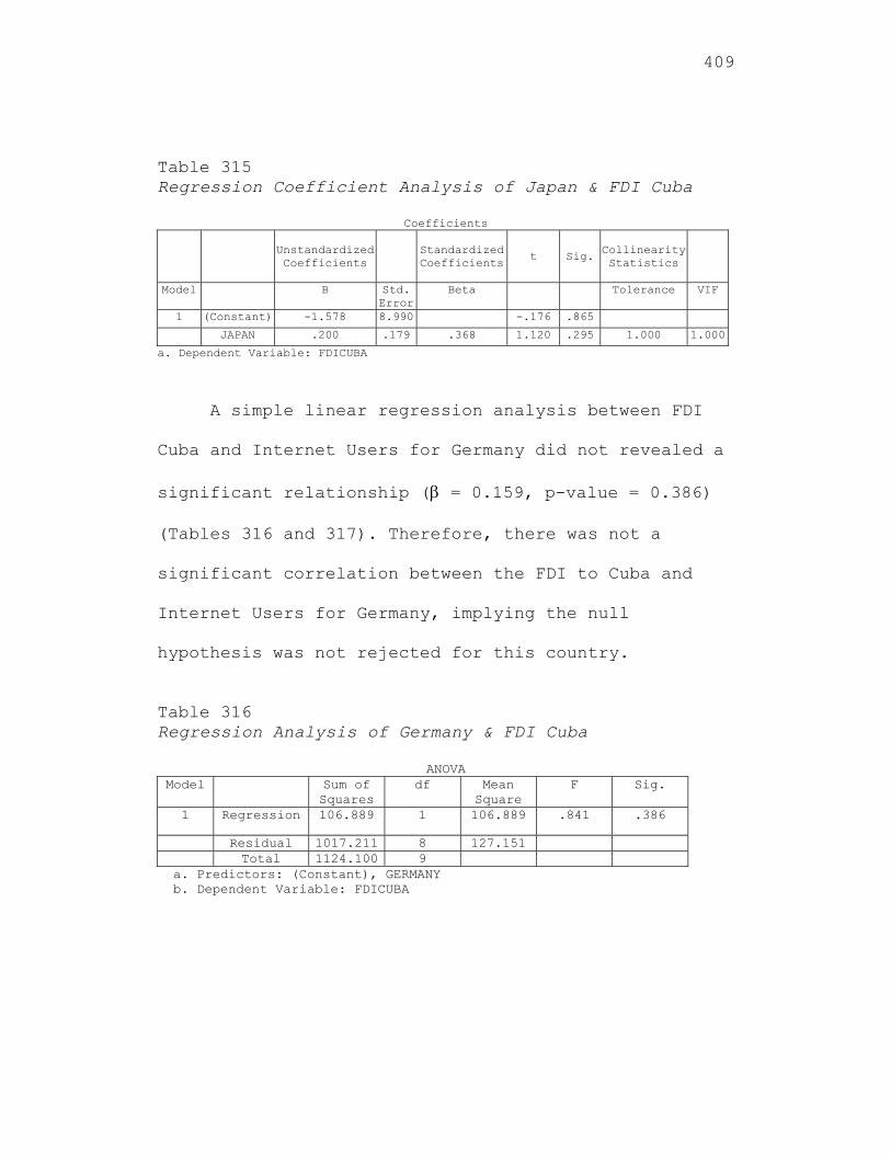
409

Table 315 Regression Coefficient Analysis of Japan & FDI Cuba

Coefficients

Unstandardized Coefficients

Standardized Coefficients

t Sig. Collinearity Statistics

Model B Std. Error

Beta Tolerance VIF

1 (Constant) -1.578 8.990 -.176 .865

JAPAN .200 .179 .368 1.120 .295 1.000 1.000

a. Dependent Variable: FDICUBA

A simple linear regression analysis between FDI

Cuba and Internet Users for Germany did not revealed a

significant relationship ( = 0.159, p-value = 0.386)

(Tables 316 and 317). Therefore, there was not a

significant correlation between the FDI to Cuba and

Internet Users for Germany, implying the null

hypothesis was not rejected for this country.

Table 316 Regression Analysis of Germany & FDI Cuba

ANOVA Model Sum of

Squares df Mean

Square F Sig.

1 Regression 106.889 1 106.889 .841 .386

Residual 1017.211 8 127.151 Total 1124.100 9

a. Predictors: (Constant), GERMANY b. Dependent Variable: FDICUBA

410

Table 317 Regression Coefficient Analysis of Germany & FDI Cuba

Coefficients

Unstandardized Coefficients

Standardized Coefficients

t Sig. Collinearity Statistics

Model B Std. Error

Beta Tolerance VIF

1 (Constant) .345 8.778 .039 .970 GERMANY .159 .173 .308 .917 .386 1.000 1.000

a. Dependent Variable: FDICUBA

A simple linear regression analysis between FDI

Cuba and Internet Users for France did not revealed a

significant relationship ( = 0.263, p-value = 0.276)

(Tables 318 and 319). Therefore, there was not a

significant correlation between the FDI to Cuba and

Internet Users for France, implying the null

hypothesis was not rejected for this country.

Table 318 Regression Analysis of France & FDI Cuba

ANOVA Model Sum of

Squares df Mean

Square F Sig.

1 Regression 164.345 1 164.345 1.370 .276

Residual 959.755 8 119.969 Total 1124.100 9

a. Predictors: (Constant), FRANCE b. Dependent Variable: FDICUBA

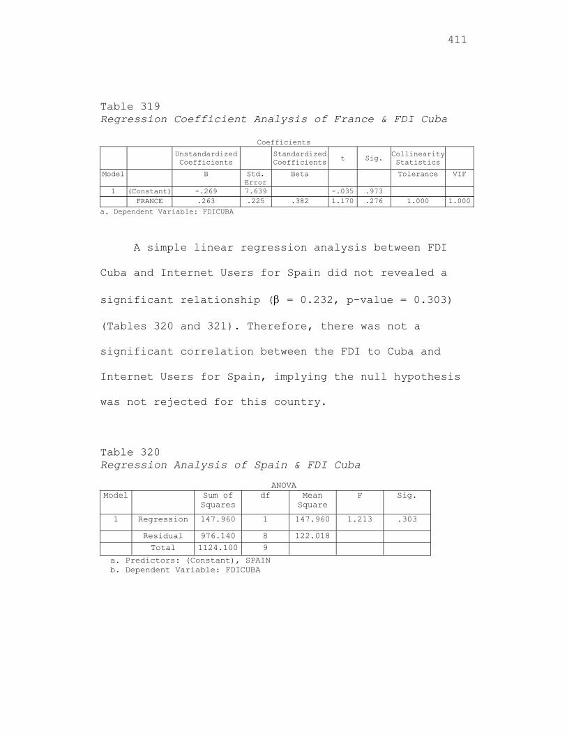
411

Table 319 Regression Coefficient Analysis of France & FDI Cuba

Coefficients Unstandardized

Coefficients Standardized Coefficients t Sig.

Collinearity Statistics

Model B Std. Error

Beta Tolerance VIF

1 (Constant) -.269 7.639 -.035 .973 FRANCE .263 .225 .382 1.170 .276 1.000 1.000

a. Dependent Variable: FDICUBA

A simple linear regression analysis between FDI

Cuba and Internet Users for Spain did not revealed a

significant relationship ( = 0.232, p-value = 0.303)

(Tables 320 and 321). Therefore, there was not a

significant correlation between the FDI to Cuba and

Internet Users for Spain, implying the null hypothesis

was not rejected for this country.

Table 320 Regression Analysis of Spain & FDI Cuba

ANOVA Model Sum of

Squares df Mean

Square F Sig.

1 Regression 147.960 1 147.960 1.213 .303

Residual 976.140 8 122.018 Total 1124.100 9

a. Predictors: (Constant), SPAIN b. Dependent Variable: FDICUBA

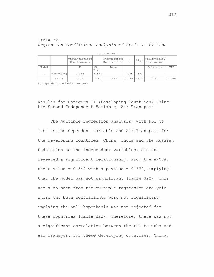
412

Table 321 Regression Coefficient Analysis of Spain & FDI Cuba

Coefficients

Unstandardized Coefficients

Standardized Coefficients

t Sig. Collinearity Statistics

Model B Std. Error

Beta Tolerance VIF

1 (Constant) 1.156 6.893 .168 .871

SPAIN .232 .211 .363 1.101 .303 1.000 1.000

a. Dependent Variable: FDICUBA

Results for Category II (Developing Countries) Using the Second Independent Variable, Air Transport

The multiple regression analysis, with FDI to

Cuba as the dependent variable and Air Transport for

the developing countries, China, India and the Russian

Federation as the independent variables, did not

revealed a significant relationship. From the ANOVA,

the F-value = 0.542 with a p-value = 0.679, implying

that the model was not significant (Table 322). This

was also seen from the multiple regression analysis

where the beta coefficients were not significant,

implying the null hypothesis was not rejected for

these countries (Table 323). Therefore, there was not

a significant correlation between the FDI to Cuba and

Air Transport for these developing countries, China,

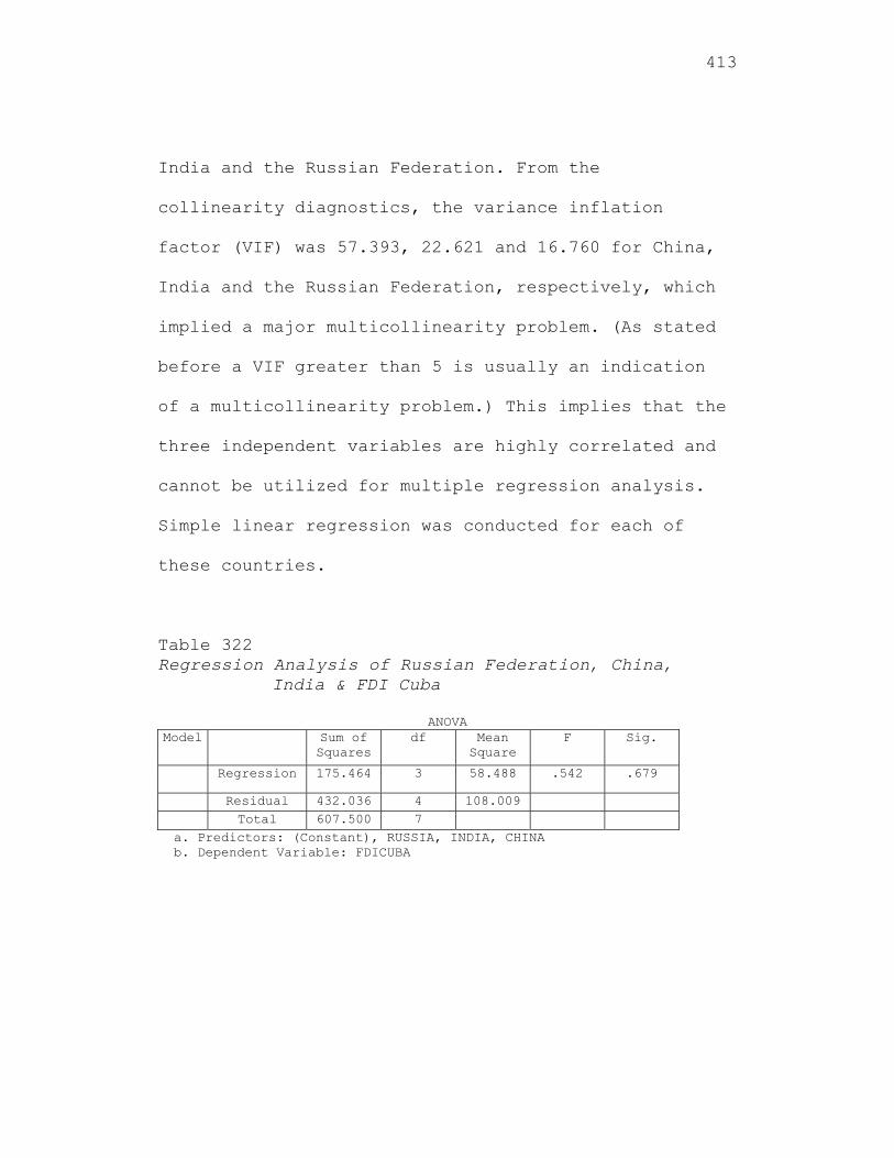
413

India and the Russian Federation. From the

collinearity diagnostics, the variance inflation

factor (VIF) was 57.393, 22.621 and 16.760 for China,

India and the Russian Federation, respectively, which

implied a major multicollinearity problem. (As stated

before a VIF greater than 5 is usually an indication

of a multicollinearity problem.) This implies that the

three independent variables are highly correlated and

cannot be utilized for multiple regression analysis.

Simple linear regression was conducted for each of

these countries.

Table 322 Regression Analysis of Russian Federation, China,

India & FDI Cuba

ANOVA Model Sum of

Squares df Mean

Square F Sig.

Regression 175.464 3 58.488 .542 .679

Residual 432.036 4 108.009 Total 607.500 7

a. Predictors: (Constant), RUSSIA, INDIA, CHINA b. Dependent Variable: FDICUBA

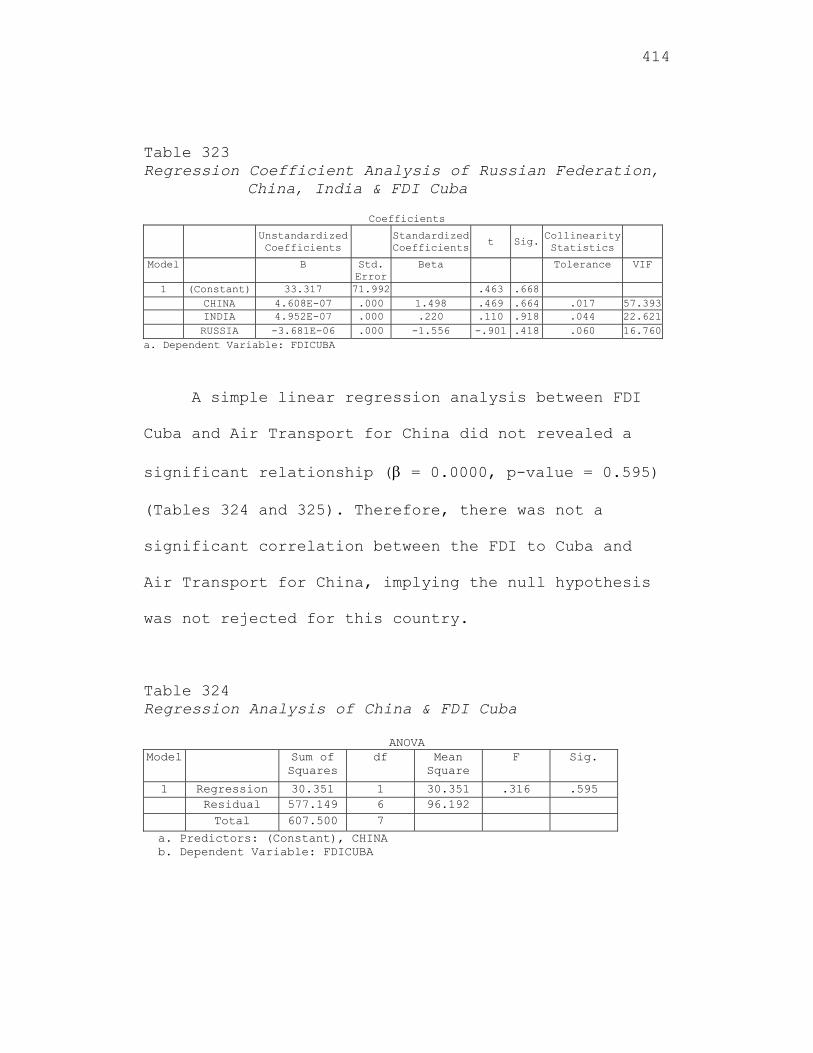
414

Table 323 Regression Coefficient Analysis of Russian Federation,

China, India & FDI Cuba

Coefficients Unstandardized

Coefficients Standardized

Coefficientst Sig. Collinearity

Statistics

Model B Std. Error

Beta Tolerance VIF

1 (Constant) 33.317 71.992 .463 .668 CHINA 4.608E-07 .000 1.498 .469 .664 .017 57.393 INDIA 4.952E-07 .000 .220 .110 .918 .044 22.621 RUSSIA -3.681E-06 .000 -1.556 -.901 .418 .060 16.760

a. Dependent Variable: FDICUBA

A simple linear regression analysis between FDI

Cuba and Air Transport for China did not revealed a

significant relationship ( = 0.0000, p-value = 0.595)

(Tables 324 and 325). Therefore, there was not a

significant correlation between the FDI to Cuba and

Air Transport for China, implying the null hypothesis

was not rejected for this country.

Table 324 Regression Analysis of China & FDI Cuba

ANOVA Model Sum of

Squares df Mean

Square F Sig.

1 Regression 30.351 1 30.351 .316 .595 Residual 577.149 6 96.192 Total 607.500 7

a. Predictors: (Constant), CHINA b. Dependent Variable: FDICUBA

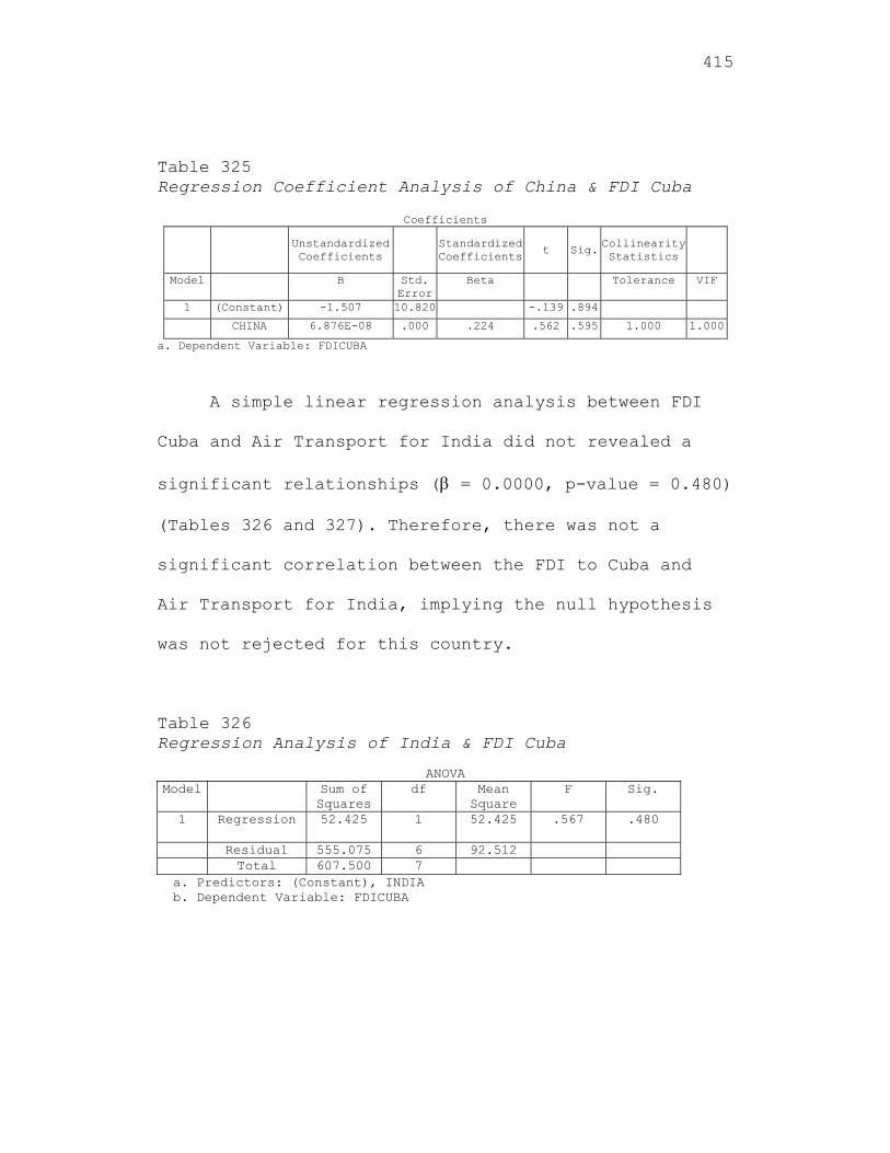
415

Table 325 Regression Coefficient Analysis of China & FDI Cuba

Coefficients

Unstandardized Coefficients

Standardized Coefficients t Sig.

Collinearity Statistics

Model B Std. Error

Beta Tolerance VIF

1 (Constant) -1.507 10.820 -.139 .894

CHINA 6.876E-08 .000 .224 .562 .595 1.000 1.000

a. Dependent Variable: FDICUBA

A simple linear regression analysis between FDI

Cuba and Air Transport for India did not revealed a

significant relationships ( = 0.0000, p-value = 0.480)

(Tables 326 and 327). Therefore, there was not a

significant correlation between the FDI to Cuba and

Air Transport for India, implying the null hypothesis

was not rejected for this country.

Table 326 Regression Analysis of India & FDI Cuba

ANOVA Model Sum of

Squares df Mean

Square F Sig.

1 Regression 52.425 1 52.425 .567 .480

Residual 555.075 6 92.512 Total 607.500 7

a. Predictors: (Constant), INDIA b. Dependent Variable: FDICUBA

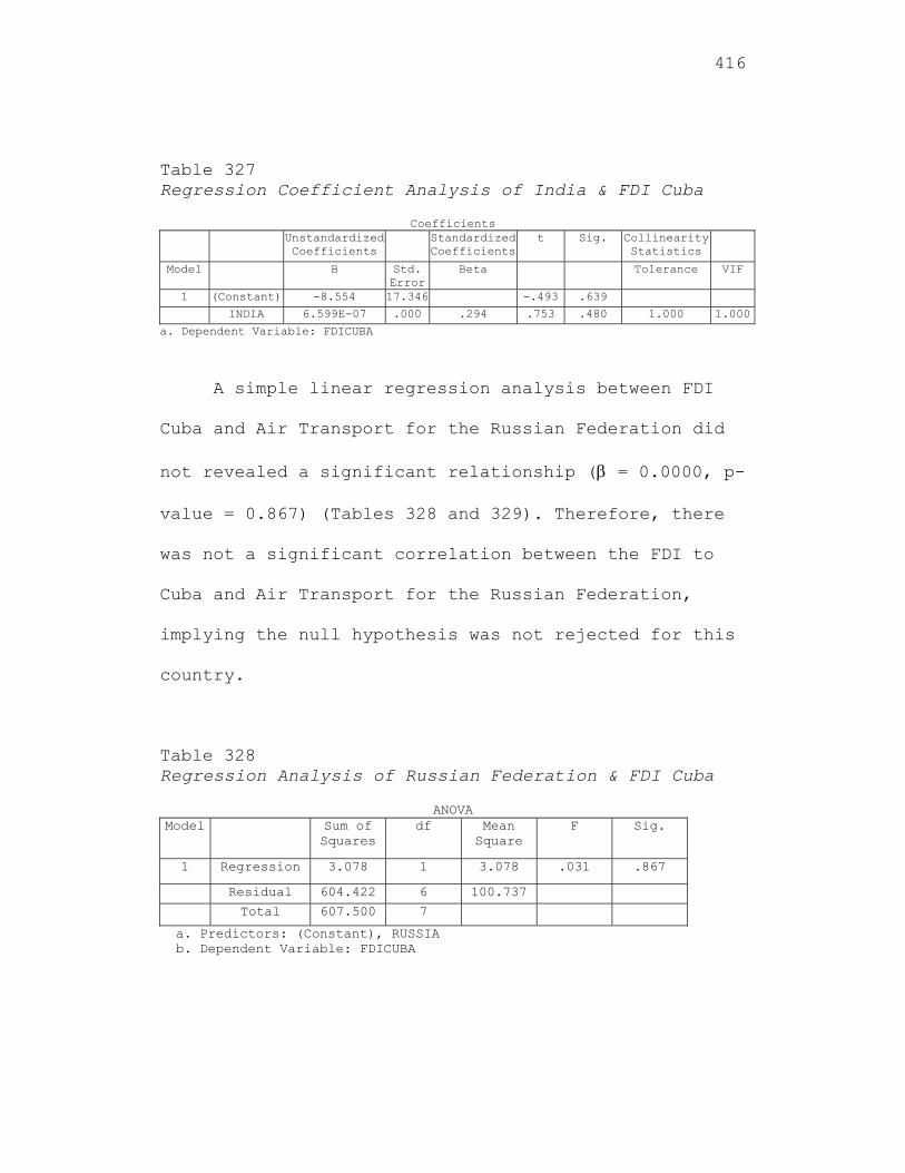
416

Table 327 Regression Coefficient Analysis of India & FDI Cuba

Coefficients Unstandardized

Coefficients Standardized

Coefficientst Sig. Collinearity

Statistics

Model B Std. Error

Beta Tolerance VIF

1 (Constant) -8.554 17.346 -.493 .639

INDIA 6.599E-07 .000 .294 .753 .480 1.000 1.000

a. Dependent Variable: FDICUBA

A simple linear regression analysis between FDI

Cuba and Air Transport for the Russian Federation did

not revealed a significant relationship ( = 0.0000, p-

value = 0.867) (Tables 328 and 329). Therefore, there

was not a significant correlation between the FDI to

Cuba and Air Transport for the Russian Federation,

implying the null hypothesis was not rejected for this

country.

Table 328 Regression Analysis of Russian Federation & FDI Cuba

ANOVA Model Sum of

Squares df Mean

Square F Sig.

1 Regression 3.078 1 3.078 .031 .867

Residual 604.422 6 100.737

Total 607.500 7

a. Predictors: (Constant), RUSSIA b. Dependent Variable: FDICUBA

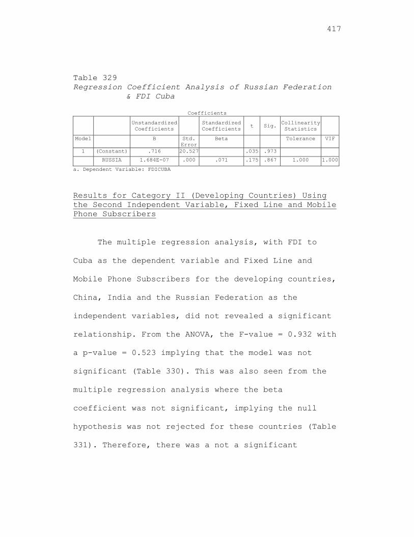
417

Table 329 Regression Coefficient Analysis of Russian Federation

& FDI Cuba

Coefficients

Unstandardized Coefficients

Standardized Coefficients

t Sig. Collinearity Statistics

Model B Std. Error

Beta Tolerance VIF

1 (Constant) .716 20.527 .035 .973

RUSSIA 1.684E-07 .000 .071 .175 .867 1.000 1.000

a. Dependent Variable: FDICUBA

Results for Category II (Developing Countries) Using the Second Independent Variable, Fixed Line and Mobile Phone Subscribers

The multiple regression analysis, with FDI to

Cuba as the dependent variable and Fixed Line and

Mobile Phone Subscribers for the developing countries,

China, India and the Russian Federation as the

independent variables, did not revealed a significant

relationship. From the ANOVA, the F-value = 0.932 with

a p-value = 0.523 implying that the model was not

significant (Table 330). This was also seen from the

multiple regression analysis where the beta

coefficient was not significant, implying the null

hypothesis was not rejected for these countries (Table

331). Therefore, there was a not a significant

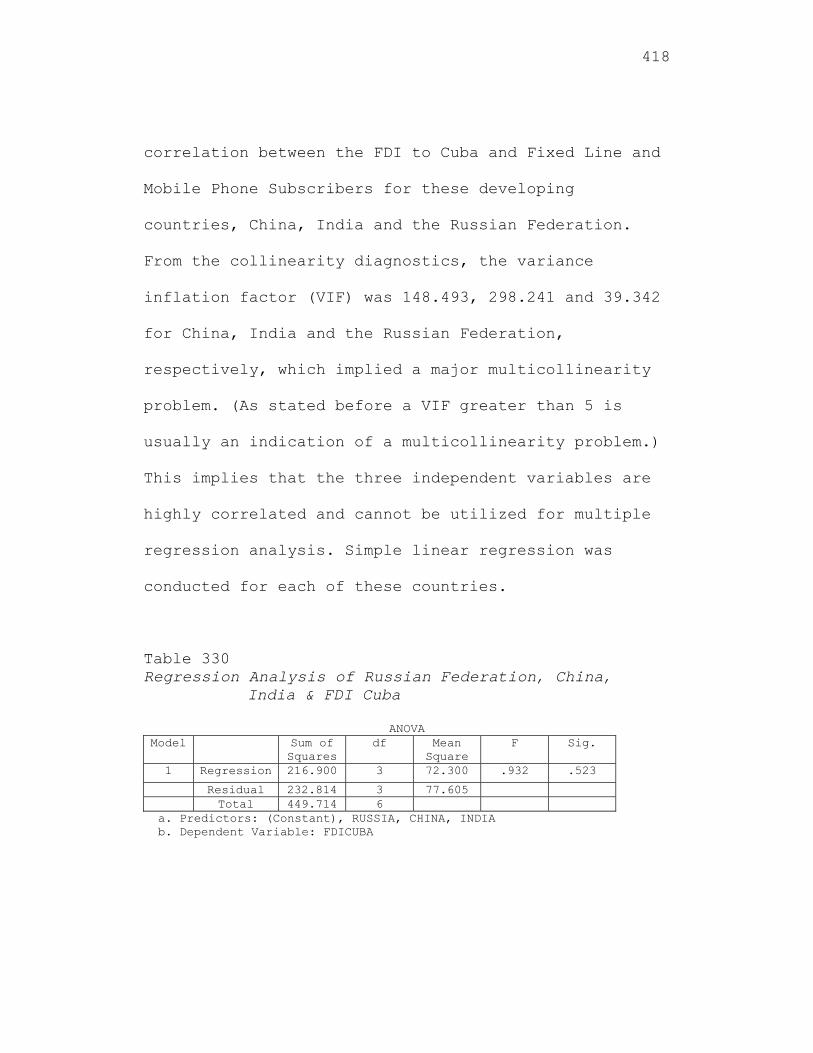
418

correlation between the FDI to Cuba and Fixed Line and

Mobile Phone Subscribers for these developing

countries, China, India and the Russian Federation.

From the collinearity diagnostics, the variance

inflation factor (VIF) was 148.493, 298.241 and 39.342

for China, India and the Russian Federation,

respectively, which implied a major multicollinearity

problem. (As stated before a VIF greater than 5 is

usually an indication of a multicollinearity problem.)

This implies that the three independent variables are

highly correlated and cannot be utilized for multiple

regression analysis. Simple linear regression was

conducted for each of these countries.

Table 330 Regression Analysis of Russian Federation, China,

India & FDI Cuba

ANOVA Model Sum of

Squares df Mean

Square F Sig.

1 Regression 216.900 3 72.300 .932 .523

Residual 232.814 3 77.605 Total 449.714 6

a. Predictors: (Constant), RUSSIA, CHINA, INDIA b. Dependent Variable: FDICUBA

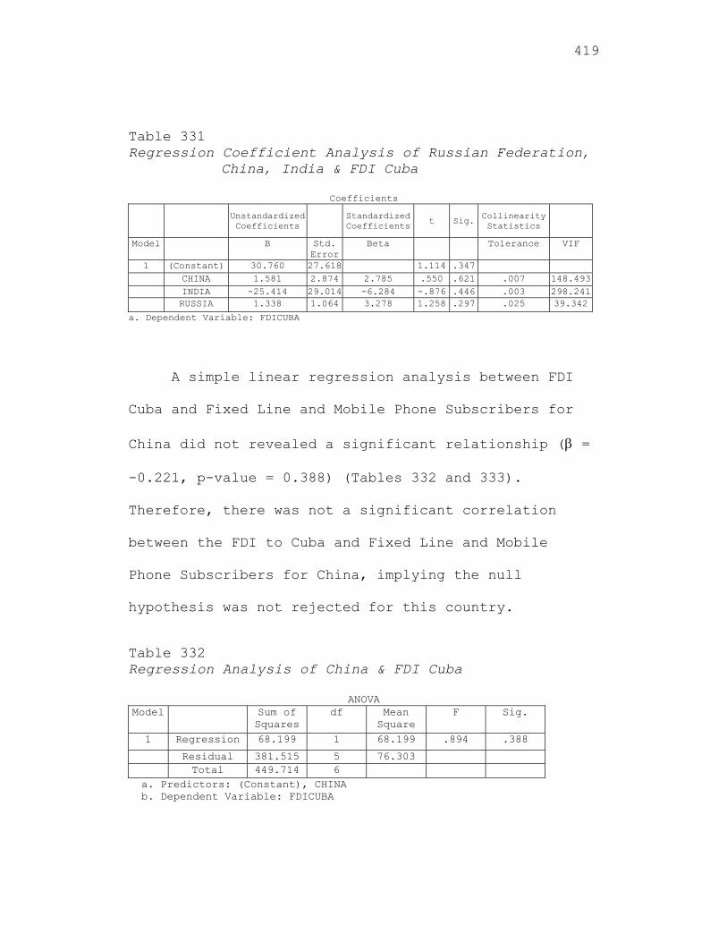
419

Table 331 Regression Coefficient Analysis of Russian Federation,

China, India & FDI Cuba

Coefficients

Unstandardized Coefficients

Standardized Coefficients

t Sig.Collinearity Statistics

Model B Std. Error

Beta Tolerance VIF

1 (Constant) 30.760 27.618 1.114 .347 CHINA 1.581 2.874 2.785 .550 .621 .007 148.493 INDIA -25.414 29.014 -6.284 -.876 .446 .003 298.241 RUSSIA 1.338 1.064 3.278 1.258 .297 .025 39.342

a. Dependent Variable: FDICUBA

A simple linear regression analysis between FDI

Cuba and Fixed Line and Mobile Phone Subscribers for

China did not revealed a significant relationship ( =

-0.221, p-value = 0.388) (Tables 332 and 333).

Therefore, there was not a significant correlation

between the FDI to Cuba and Fixed Line and Mobile

Phone Subscribers for China, implying the null

hypothesis was not rejected for this country.

Table 332 Regression Analysis of China & FDI Cuba

ANOVA Model Sum of

Squares df Mean

Square F Sig.

1 Regression 68.199 1 68.199 .894 .388

Residual 381.515 5 76.303 Total 449.714 6

a. Predictors: (Constant), CHINA b. Dependent Variable: FDICUBA

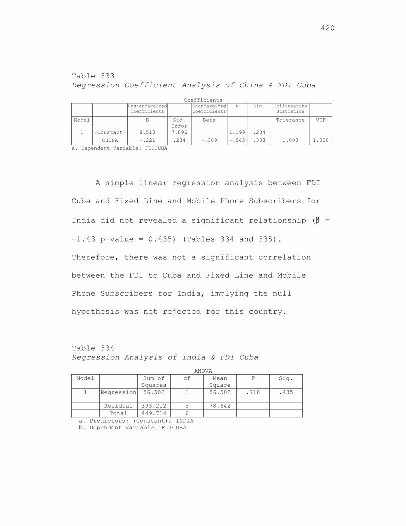
420

Table 333 Regression Coefficient Analysis of China & FDI Cuba

Coefficients Unstandardized

Coefficients Standardized

Coefficientst Sig. Collinearity

Statistics

Model B Std. Error

Beta Tolerance VIF

1 (Constant) 8.510 7.096 1.199 .284

CHINA -.221 .234 -.389 -.945 .388 1.000 1.000

a. Dependent Variable: FDICUBA

A simple linear regression analysis between FDI

Cuba and Fixed Line and Mobile Phone Subscribers for

India did not revealed a significant relationship ( =

-1.43 p-value = 0.435) (Tables 334 and 335).

Therefore, there was not a significant correlation

between the FDI to Cuba and Fixed Line and Mobile

Phone Subscribers for India, implying the null

hypothesis was not rejected for this country.

Table 334 Regression Analysis of India & FDI Cuba

ANOVA Model Sum of

Squares df Mean

Square F Sig.

1 Regression 56.502 1 56.502 .718 .435

Residual 393.212 5 78.642 Total 449.714 6

a. Predictors: (Constant), INDIA b. Dependent Variable: FDICUBA

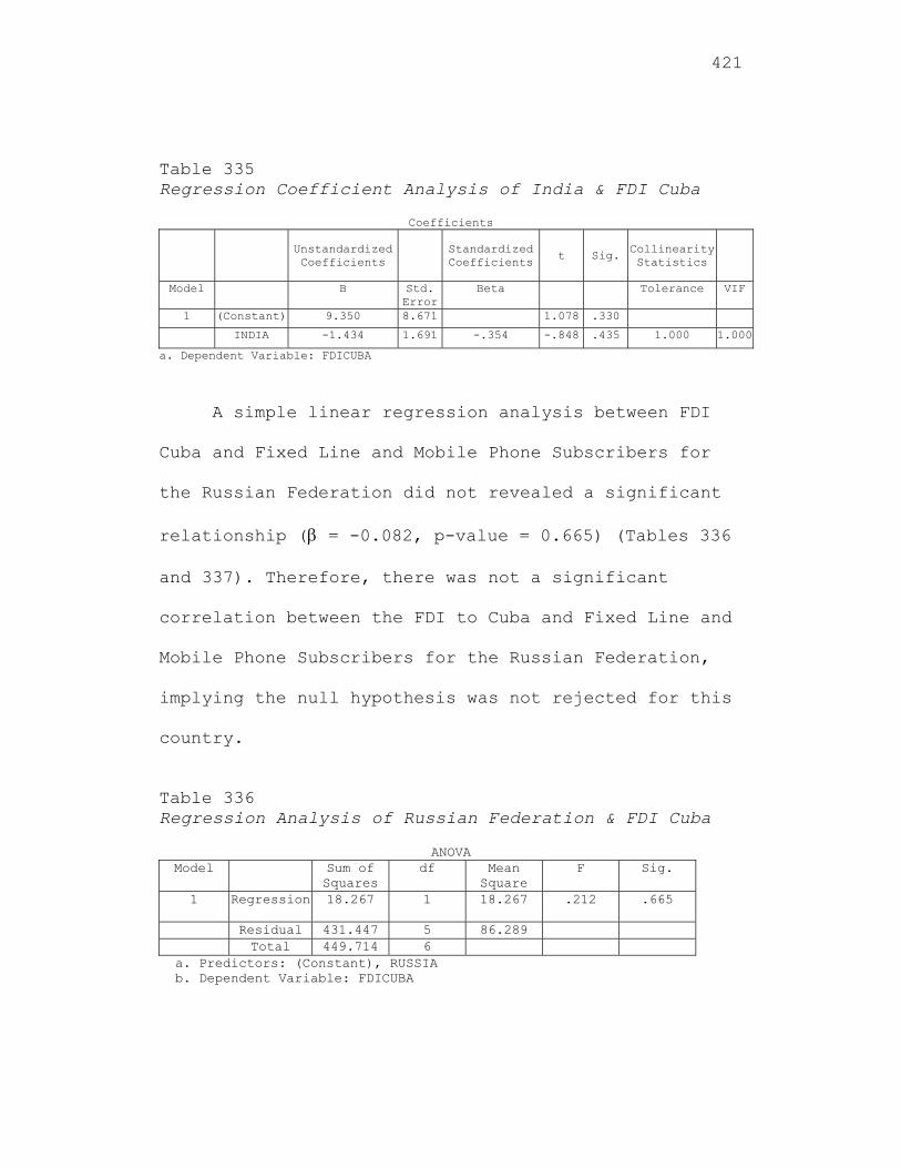
421

Table 335 Regression Coefficient Analysis of India & FDI Cuba

Coefficients

Unstandardized Coefficients

Standardized Coefficients

t Sig. Collinearity Statistics

Model B Std. Error

Beta Tolerance VIF

1 (Constant) 9.350 8.671 1.078 .330

INDIA -1.434 1.691 -.354 -.848 .435 1.000 1.000

a. Dependent Variable: FDICUBA

A simple linear regression analysis between FDI

Cuba and Fixed Line and Mobile Phone Subscribers for

the Russian Federation did not revealed a significant

relationship ( = -0.082, p-value = 0.665) (Tables 336

and 337). Therefore, there was not a significant

correlation between the FDI to Cuba and Fixed Line and

Mobile Phone Subscribers for the Russian Federation,

implying the null hypothesis was not rejected for this

country.

Table 336 Regression Analysis of Russian Federation & FDI Cuba

ANOVA Model Sum of

Squares df Mean

Square F Sig.

1 Regression 18.267 1 18.267 .212 .665

Residual 431.447 5 86.289 Total 449.714 6

a. Predictors: (Constant), RUSSIA b. Dependent Variable: FDICUBA

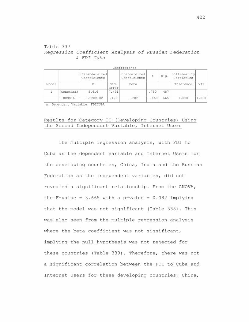
422

Table 337 Regression Coefficient Analysis of Russian Federation

& FDI Cuba

Coefficients

Unstandardized Coefficients

Standardized Coefficients t Sig.

Collinearity Statistics

Model B Std. Error

Beta Tolerance VIF

1 (Constant) 5.616 7.491 .750 .487

RUSSIA -8.228E-02 .179 -.202 -.460 .665 1.000 1.000

a. Dependent Variable: FDICUBA

Results for Category II (Developing Countries) Using the Second Independent Variable, Internet Users

The multiple regression analysis, with FDI to

Cuba as the dependent variable and Internet Users for

the developing countries, China, India and the Russian

Federation as the independent variables, did not

revealed a significant relationship. From the ANOVA,

the F-value = 3.665 with a p-value = 0.082 implying

that the model was not significant (Table 338). This

was also seen from the multiple regression analysis

where the beta coefficient was not significant,

implying the null hypothesis was not rejected for

these countries (Table 339). Therefore, there was not

a significant correlation between the FDI to Cuba and

Internet Users for these developing countries, China,

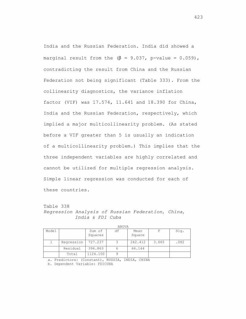
423

India and the Russian Federation. India did showed a

marginal result from the ( = 9.037, p-value = 0.059),

contradicting the result from China and the Russian

Federation not being significant (Table 333). From the

collinearity diagnostics, the variance inflation

factor (VIF) was 17.574, 11.641 and 18.390 for China,

India and the Russian Federation, respectively, which

implied a major multicollinearity problem. (As stated

before a VIF greater than 5 is usually an indication

of a multicollinearity problem.) This implies that the

three independent variables are highly correlated and

cannot be utilized for multiple regression analysis.

Simple linear regression was conducted for each of

these countries.

Table 338 Regression Analysis of Russian Federation, China,

India & FDI Cuba

ANOVA Model Sum of

Squares df Mean

Square F Sig.

1 Regression 727.237 3 242.412 3.665 .082

Residual 396.863 6 66.144

Total 1124.100 9

a. Predictors: (Constant), RUSSIA, INDIA, CHINA b. Dependent Variable: FDICUBA

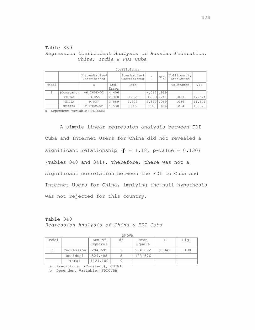
424

Table 339 Regression Coefficient Analysis of Russian Federation,

China, India & FDI Cuba

Coefficients

Unstandardized Coefficients

Standardized Coefficients t Sig.

Collinearity Statistics

Model B Std. Error

Beta Tolerance VIF

1 (Constant) -6.265E-02 4.406 -.014 .989 CHINA -3.055 2.348 -1.323 -1.301 .241 .057 17.574 INDIA 9.037 3.889 1.923 2.324 .059 .086 11.641 RUSSIA 2.239E-02 1.538 .015 .015 .989 .054 18.390

a. Dependent Variable: FDICUBA

A simple linear regression analysis between FDI

Cuba and Internet Users for China did not revealed a

significant relationship ( = 1.18, p-value = 0.130)

(Tables 340 and 341). Therefore, there was not a

significant correlation between the FDI to Cuba and

Internet Users for China, implying the null hypothesis

was not rejected for this country.

Table 340 Regression Analysis of China & FDI Cuba

ANOVA Model Sum of

Squares df Mean

Square F Sig.

1 Regression 294.692 1 294.692 2.842 .130

Residual 829.408 8 103.676 Total 1124.100 9

a. Predictors: (Constant), CHINA b. Dependent Variable: FDICUBA

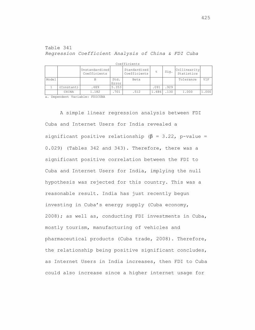
425

Table 341 Regression Coefficient Analysis of China & FDI Cuba

Coefficients

Unstandardized Coefficients

Standardized Coefficients t Sig.

Collinearity Statistics

Model B Std. Error

Beta Tolerance VIF

1 (Constant) .489 5.353 .091 .929 CHINA 1.182 .701 .512 1.686 .130 1.000 1.000

a. Dependent Variable: FDICUBA

A simple linear regression analysis between FDI

Cuba and Internet Users for India revealed a

significant positive relationship ( = 3.22, p-value =

0.029) (Tables 342 and 343). Therefore, there was a

significant positive correlation between the FDI to

Cuba and Internet Users for India, implying the null

hypothesis was rejected for this country. This was a

reasonable result. India has just recently begun

investing in Cuba’s energy supply (Cuba economy,

2008); as well as, conducting FDI investments in Cuba,

mostly tourism, manufacturing of vehicles and

pharmaceutical products (Cuba trade, 2008). Therefore,

the relationship being positive significant concludes,

as Internet Users in India increases, then FDI to Cuba

could also increase since a higher internet usage for

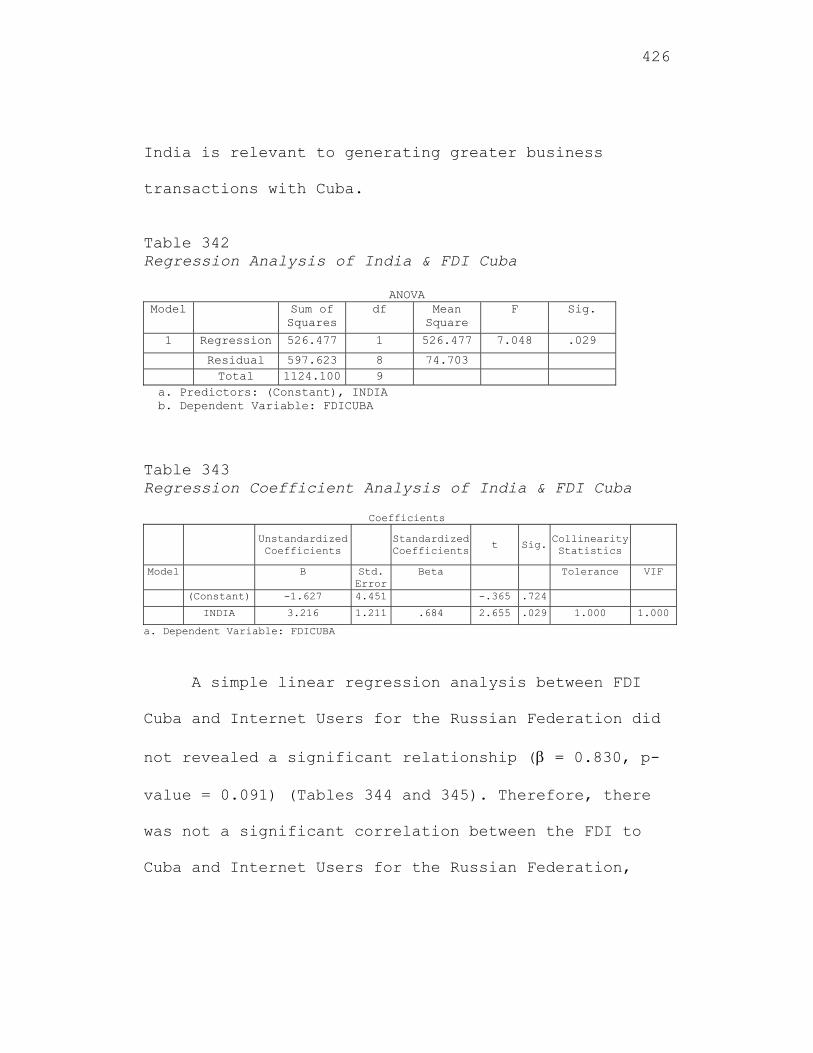
426

India is relevant to generating greater business

transactions with Cuba.

Table 342 Regression Analysis of India & FDI Cuba

ANOVA Model Sum of

Squares df Mean

Square F Sig.

1 Regression 526.477 1 526.477 7.048 .029

Residual 597.623 8 74.703 Total 1124.100 9

a. Predictors: (Constant), INDIA b. Dependent Variable: FDICUBA

Table 343 Regression Coefficient Analysis of India & FDI Cuba

Coefficients

Unstandardized Coefficients

Standardized Coefficients t Sig.

Collinearity Statistics

Model B Std. Error

Beta Tolerance VIF

(Constant) -1.627 4.451 -.365 .724

INDIA 3.216 1.211 .684 2.655 .029 1.000 1.000

a. Dependent Variable: FDICUBA

A simple linear regression analysis between FDI

Cuba and Internet Users for the Russian Federation did

not revealed a significant relationship ( = 0.830, p-

value = 0.091) (Tables 344 and 345). Therefore, there

was not a significant correlation between the FDI to

Cuba and Internet Users for the Russian Federation,

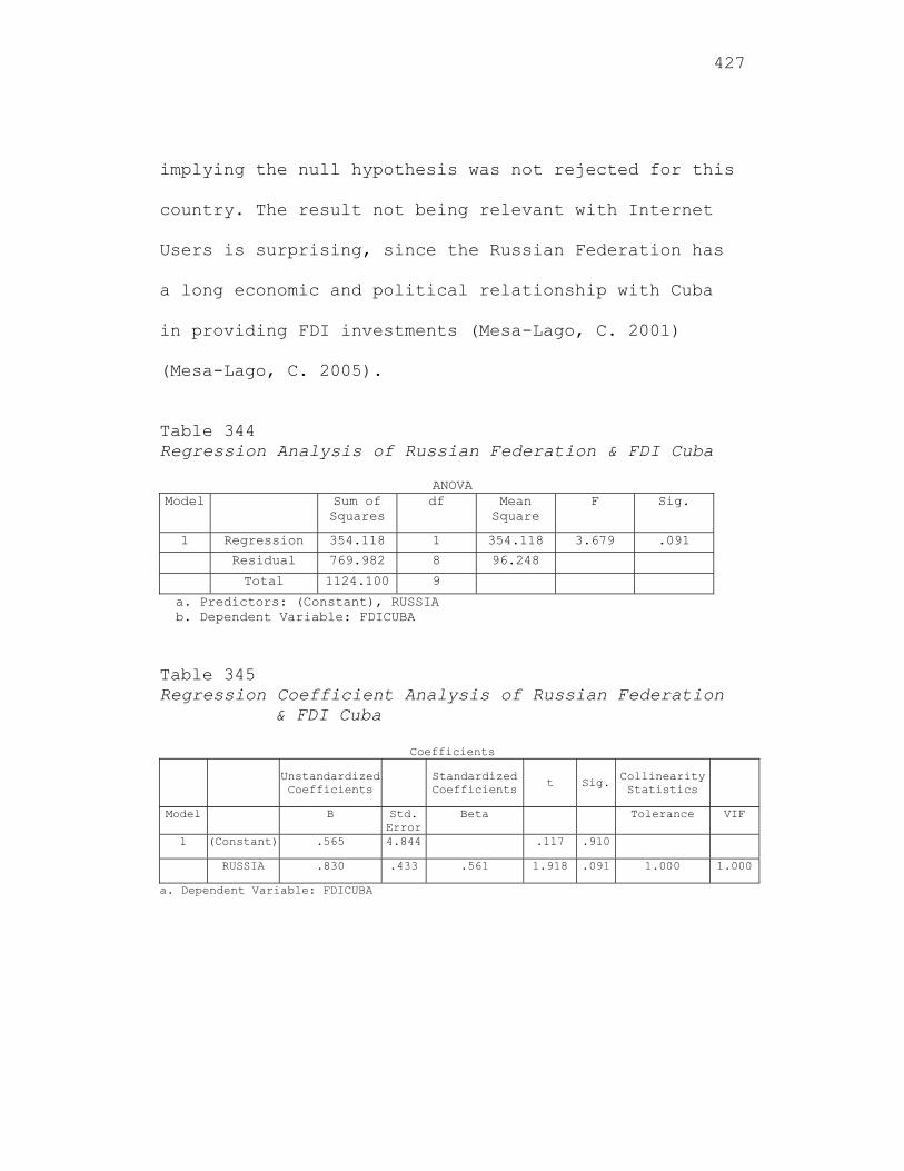
427

implying the null hypothesis was not rejected for this

country. The result not being relevant with Internet

Users is surprising, since the Russian Federation has

a long economic and political relationship with Cuba

in providing FDI investments (Mesa-Lago, C. 2001)

(Mesa-Lago, C. 2005).

Table 344 Regression Analysis of Russian Federation & FDI Cuba

ANOVA Model Sum of

Squares df Mean

Square F Sig.

1 Regression 354.118 1 354.118 3.679 .091

Residual 769.982 8 96.248

Total 1124.100 9

a. Predictors: (Constant), RUSSIA b. Dependent Variable: FDICUBA

Table 345 Regression Coefficient Analysis of Russian Federation

& FDI Cuba

Coefficients

Unstandardized Coefficients

Standardized Coefficients

t Sig. Collinearity Statistics

Model B Std. Error

Beta Tolerance VIF

1 (Constant) .565 4.844 .117 .910

RUSSIA .830 .433 .561 1.918 .091 1.000 1.000

a. Dependent Variable: FDICUBA

428

Results for Category III (Least Developed Countries) Using the Third Independent Variable, Air Transport

For the third category of countries, multiple

regression analysis was done for FDI to Cuba as the

dependent variable and Air Transport for the least

Developing countries, Jamaica, Peru, Madagascar and

Nepal as the independent variables. Haiti was not

tested based on insufficient data. This analysis did

not revealed a significant relationships with FDI to

Cuba (F value = 1.860 with a p-value = 0.319) (Table

346). Again, the beta coefficients were not

significant, implying the null hypothesis was not

rejected for these countries (Table 347). Therefore,

there was not a significant correlation between the

FDI to Cuba and Air Transport for the least developing

countries of Jamaica, Peru, Madagascar and Nepal.

Surprisingly, all four countries did not have a

correlation problem based on their VIF (variance

inflation factor) of 1.901, 1.578, 2.923 and 3.776 for

Jamaica, Peru, Madagascar and Nepal, respectively.

(VIF greater than 5 is usually an indication of a

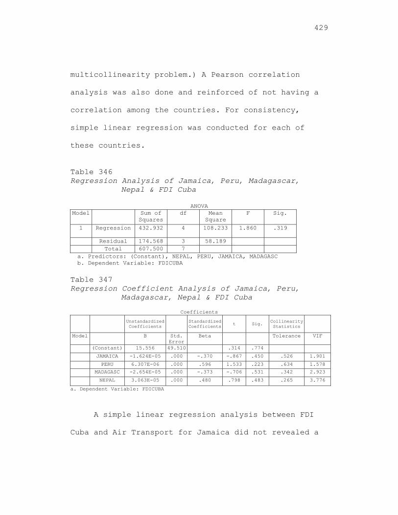
429

multicollinearity problem.) A Pearson correlation

analysis was also done and reinforced of not having a

correlation among the countries. For consistency,

simple linear regression was conducted for each of

these countries.

Table 346 Regression Analysis of Jamaica, Peru, Madagascar,

Nepal & FDI Cuba

ANOVA Model Sum of

Squares df Mean

Square F Sig.

1 Regression 432.932 4 108.233 1.860 .319

Residual 174.568 3 58.189 Total 607.500 7

a. Predictors: (Constant), NEPAL, PERU, JAMAICA, MADAGASC b. Dependent Variable: FDICUBA Table 347 Regression Coefficient Analysis of Jamaica, Peru,

Madagascar, Nepal & FDI Cuba

Coefficients

Unstandardized Coefficients Standardized

Coefficients t Sig. Collinearity Statistics

Model B Std. Error

Beta Tolerance VIF

(Constant) 15.556 49.510 .314 .774

JAMAICA -1.624E-05 .000 -.370 -.867 .450 .526 1.901

PERU 6.307E-06 .000 .596 1.533 .223 .634 1.578

MADAGASC -2.654E-05 .000 -.373 -.706 .531 .342 2.923

NEPAL 3.063E-05 .000 .480 .798 .483 .265 3.776

a. Dependent Variable: FDICUBA

A simple linear regression analysis between FDI

Cuba and Air Transport for Jamaica did not revealed a

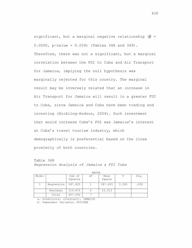
430

significant, but a marginal negative relationship ( =

0.0000, p-value = 0.059) (Tables 348 and 349).

Therefore, there was not a significant, but a marginal

correlation between the FDI to Cuba and Air Transport

for Jamaica, implying the null hypothesis was

marginally rejected for this country. The marginal

result may be inversely related that an increase in

Air Transport for Jamaica will result in a greater FDI

to Cuba, since Jamaica and Cuba have been trading and

investing (Hickling-Hudson, 2004). Such investment

that would increase Cuba’s FDI was Jamaica’s interest

at Cuba’s travel tourism industry, which

demographically is preferential based on the close

proximity of both countries.

Table 348 Regression Analysis of Jamaica & FDI Cuba

ANOVA Model Sum of

Squares df Mean

Square F Sig.

1 Regression 287.625 1 287.625 5.395 .059

Residual 319.875 6 53.313

Total 607.500 7

a. Predictors: (Constant), JAMAICA b. Dependent Variable: FDICUBA

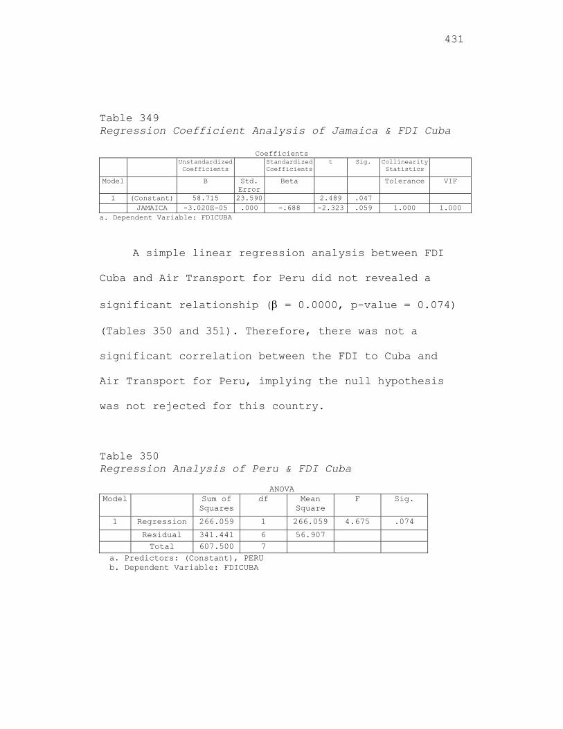
431

Table 349 Regression Coefficient Analysis of Jamaica & FDI Cuba

Coefficients Unstandardized

Coefficients Standardized

Coefficientst Sig. Collinearity

Statistics

Model B Std. Error

Beta Tolerance VIF

1 (Constant) 58.715 23.590 2.489 .047 JAMAICA -3.020E-05 .000 -.688 -2.323 .059 1.000 1.000

a. Dependent Variable: FDICUBA

A simple linear regression analysis between FDI

Cuba and Air Transport for Peru did not revealed a

significant relationship ( = 0.0000, p-value = 0.074)

(Tables 350 and 351). Therefore, there was not a

significant correlation between the FDI to Cuba and

Air Transport for Peru, implying the null hypothesis

was not rejected for this country.

Table 350 Regression Analysis of Peru & FDI Cuba

ANOVA

Model Sum of Squares

df Mean Square

F Sig.

1 Regression 266.059 1 266.059 4.675 .074

Residual 341.441 6 56.907 Total 607.500 7

a. Predictors: (Constant), PERU b. Dependent Variable: FDICUBA

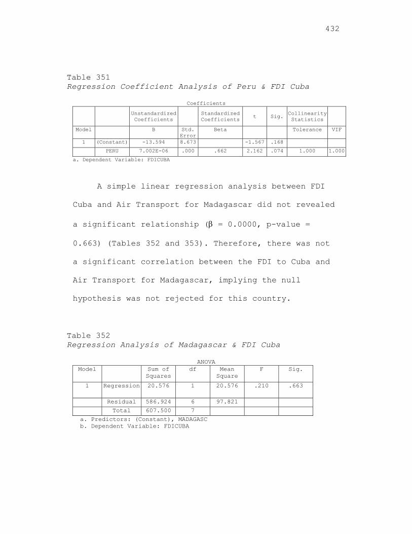
432

Table 351 Regression Coefficient Analysis of Peru & FDI Cuba

Coefficients

Unstandardized Coefficients

Standardized Coefficients

t Sig. Collinearity Statistics

Model B Std. Error

Beta Tolerance VIF

1 (Constant) -13.594 8.673 -1.567 .168

PERU 7.002E-06 .000 .662 2.162 .074 1.000 1.000

a. Dependent Variable: FDICUBA

A simple linear regression analysis between FDI

Cuba and Air Transport for Madagascar did not revealed

a significant relationship ( = 0.0000, p-value =

0.663) (Tables 352 and 353). Therefore, there was not

a significant correlation between the FDI to Cuba and

Air Transport for Madagascar, implying the null

hypothesis was not rejected for this country.

Table 352 Regression Analysis of Madagascar & FDI Cuba

ANOVA Model Sum of

Squares df Mean

Square F Sig.

1 Regression 20.576 1 20.576 .210 .663

Residual 586.924 6 97.821

Total 607.500 7

a. Predictors: (Constant), MADAGASC b. Dependent Variable: FDICUBA

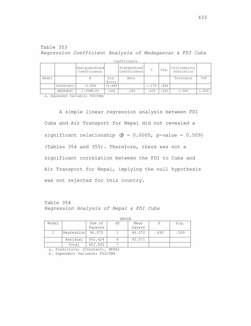
433

Table 353 Regression Coefficient Analysis of Madagascar & FDI Cuba

Coefficients

Unstandardized Coefficients

Standardized Coefficients

t Sig. Collinearity Statistics

Model B Std. Error

Beta Tolerance VIF

(Constant) -2.836 15.840 -.179 .864

MADAGASC 1.308E-05 .000 .184 .459 .663 1.000 1.000

a. Dependent Variable: FDICUBA

A simple linear regression analysis between FDI

Cuba and Air Transport for Nepal did not revealed a

significant relationship ( = 0.0000, p-value = 0.509)

(Tables 354 and 355). Therefore, there was not a

significant correlation between the FDI to Cuba and

Air Transport for Nepal, implying the null hypothesis

was not rejected for this country.

Table 354 Regression Analysis of Nepal & FDI Cuba

ANOVA Model Sum of

Squares df Mean

Square F Sig.

1 Regression 46.072 1 46.072 .492 .509

Residual 561.428 6 93.571 Total 607.500 7

a. Predictors: (Constant), NEPAL b. Dependent Variable: FDICUBA

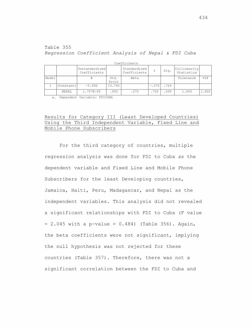
434

Table 355 Regression Coefficient Analysis of Nepal & FDI Cuba

Coefficients

Unstandardized Coefficients

Standardized Coefficients t Sig.

Collinearity Statistics

Model B Std. Error

Beta Tolerance VIF

1 (Constant) -5.092 13.745 -.370 .724

NEPAL 1.757E-05 .000 .275 .702 .509 1.000 1.000

a. Dependent Variable: FDICUBA

Results for Category III (Least Developed Countries) Using the Third Independent Variable, Fixed Line and Mobile Phone Subscribers

For the third category of countries, multiple

regression analysis was done for FDI to Cuba as the

dependent variable and Fixed Line and Mobile Phone

Subscribers for the least Developing countries,

Jamaica, Haiti, Peru, Madagascar, and Nepal as the

independent variables. This analysis did not revealed

a significant relationships with FDI to Cuba (F value

= 2.045 with a p-value = 0.484) (Table 356). Again,

the beta coefficients were not significant, implying

the null hypothesis was not rejected for these

countries (Table 357). Therefore, there was not a

significant correlation between the FDI to Cuba and

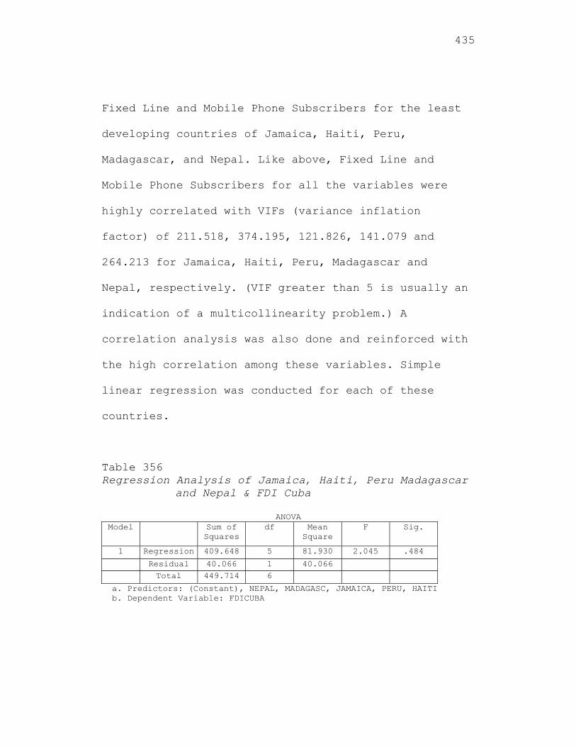
435

Fixed Line and Mobile Phone Subscribers for the least

developing countries of Jamaica, Haiti, Peru,

Madagascar, and Nepal. Like above, Fixed Line and

Mobile Phone Subscribers for all the variables were

highly correlated with VIFs (variance inflation

factor) of 211.518, 374.195, 121.826, 141.079 and

264.213 for Jamaica, Haiti, Peru, Madagascar and

Nepal, respectively. (VIF greater than 5 is usually an

indication of a multicollinearity problem.) A

correlation analysis was also done and reinforced with

the high correlation among these variables. Simple

linear regression was conducted for each of these

countries.

Table 356 Regression Analysis of Jamaica, Haiti, Peru Madagascar

and Nepal & FDI Cuba

ANOVA Model Sum of

Squares df Mean

Square F Sig.

1 Regression 409.648 5 81.930 2.045 .484

Residual 40.066 1 40.066 Total 449.714 6

a. Predictors: (Constant), NEPAL, MADAGASC, JAMAICA, PERU, HAITI b. Dependent Variable: FDICUBA

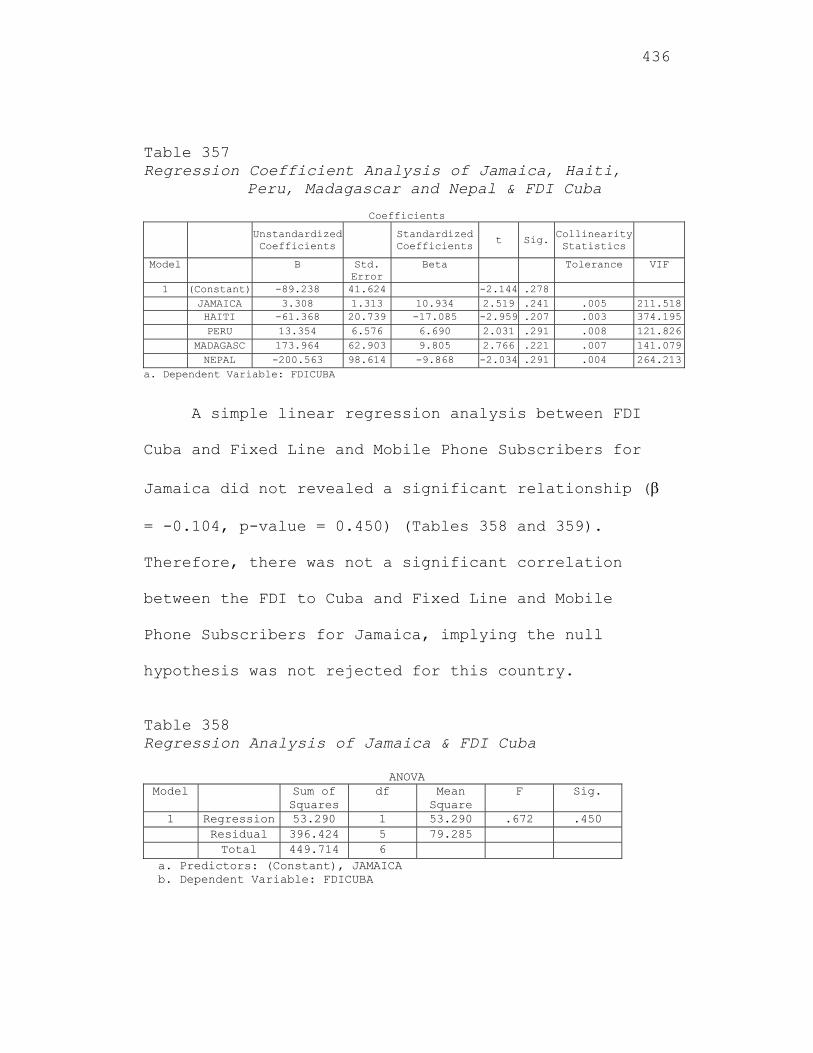
436

Table 357 Regression Coefficient Analysis of Jamaica, Haiti,

Peru, Madagascar and Nepal & FDI Cuba

Coefficients

Unstandardized Coefficients

Standardized Coefficients

t Sig. Collinearity Statistics

Model B Std. Error

Beta Tolerance VIF

1 (Constant) -89.238 41.624 -2.144 .278 JAMAICA 3.308 1.313 10.934 2.519 .241 .005 211.518 HAITI -61.368 20.739 -17.085 -2.959 .207 .003 374.195 PERU 13.354 6.576 6.690 2.031 .291 .008 121.826 MADAGASC 173.964 62.903 9.805 2.766 .221 .007 141.079 NEPAL -200.563 98.614 -9.868 -2.034 .291 .004 264.213

a. Dependent Variable: FDICUBA

A simple linear regression analysis between FDI

Cuba and Fixed Line and Mobile Phone Subscribers for

Jamaica did not revealed a significant relationship (

= -0.104, p-value = 0.450) (Tables 358 and 359).

Therefore, there was not a significant correlation

between the FDI to Cuba and Fixed Line and Mobile

Phone Subscribers for Jamaica, implying the null

hypothesis was not rejected for this country.

Table 358 Regression Analysis of Jamaica & FDI Cuba

ANOVA Model Sum of

Squares df Mean

Square F Sig.

1 Regression 53.290 1 53.290 .672 .450 Residual 396.424 5 79.285 Total 449.714 6

a. Predictors: (Constant), JAMAICA b. Dependent Variable: FDICUBA

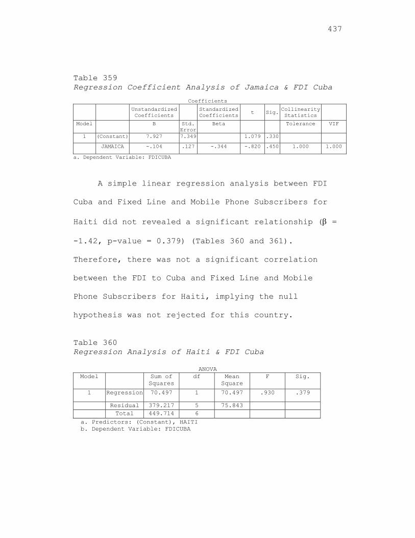
437

Table 359 Regression Coefficient Analysis of Jamaica & FDI Cuba

Coefficients

Unstandardized Coefficients

Standardized Coefficients t Sig.

Collinearity Statistics

Model B Std. Error

Beta Tolerance VIF

1 (Constant) 7.927 7.349 1.079 .330

JAMAICA -.104 .127 -.344 -.820 .450 1.000 1.000

a. Dependent Variable: FDICUBA

A simple linear regression analysis between FDI

Cuba and Fixed Line and Mobile Phone Subscribers for

Haiti did not revealed a significant relationship ( =

-1.42, p-value = 0.379) (Tables 360 and 361).

Therefore, there was not a significant correlation

between the FDI to Cuba and Fixed Line and Mobile

Phone Subscribers for Haiti, implying the null

hypothesis was not rejected for this country.

Table 360 Regression Analysis of Haiti & FDI Cuba

ANOVA Model Sum of

Squares df Mean

Square F Sig.

1 Regression 70.497 1 70.497 .930 .379

Residual 379.217 5 75.843 Total 449.714 6

a. Predictors: (Constant), HAITI b. Dependent Variable: FDICUBA

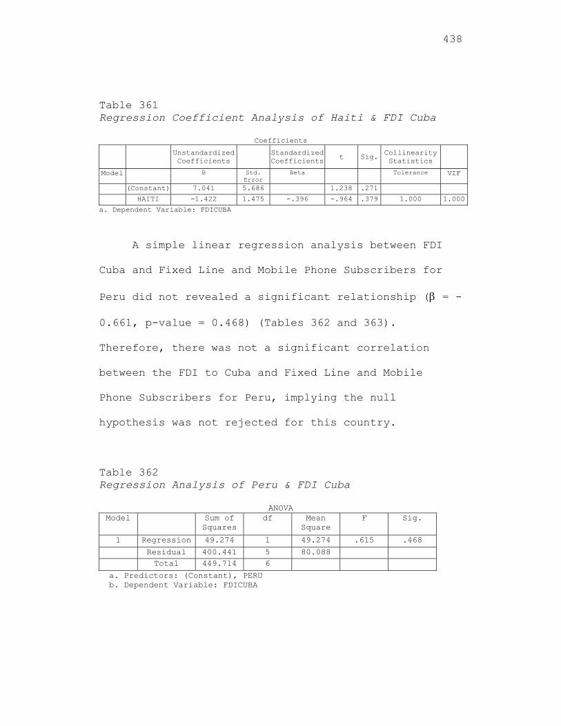
438

Table 361 Regression Coefficient Analysis of Haiti & FDI Cuba

Coefficients Unstandardized

Coefficients Standardized Coefficients t Sig.

Collinearity Statistics

Model B Std. Error

Beta Tolerance VIF

(Constant) 7.041 5.686 1.238 .271

HAITI -1.422 1.475 -.396 -.964 .379 1.000 1.000

a. Dependent Variable: FDICUBA

A simple linear regression analysis between FDI

Cuba and Fixed Line and Mobile Phone Subscribers for

Peru did not revealed a significant relationship ( = -

0.661, p-value = 0.468) (Tables 362 and 363).

Therefore, there was not a significant correlation

between the FDI to Cuba and Fixed Line and Mobile

Phone Subscribers for Peru, implying the null

hypothesis was not rejected for this country.

Table 362 Regression Analysis of Peru & FDI Cuba

ANOVA Model Sum of

Squares df Mean

Square F Sig.

1 Regression 49.274 1 49.274 .615 .468

Residual 400.441 5 80.088 Total 449.714 6

a. Predictors: (Constant), PERU b. Dependent Variable: FDICUBA

439

Table 363 Regression Coefficient Analysis of Peru & FDI Cuba

Coefficients Unstandardized

Coefficients Standardized

Coefficientst Sig. Collinearity

Statistics

Model B Std. Error

Beta Tolerance VIF

1 (Constant) 11.916 12.385 .962 .380

PERU -.661 .842 -.331 -.784 .468 1.000 1.000

a. Dependent Variable: FDICUBA

A simple linear regression analysis between FDI Cuba

and Fixed Line and Mobile Phone Subscribers for

Madagascar did not revealed a significant relationship

( = -5.70, p-value = 0.482) (Tables 364 and 365).

Therefore, there was not a significant correlation

between the FDI to Cuba and Fixed Line and Mobile

Phone Subscribers for Madagascar, implying the null

hypothesis was not rejected for this country.

Table 364 Regression Analysis of Madagascar & FDI Cuba

ANOVA Model Sum of

Squares df Mean

Square F Sig.

1 Regression 46.414 1 46.414 .575 .482

Residual 403.300 5 80.660 Total 449.714 6

a. Predictors: (Constant), MADAGASC b. Dependent Variable: FDICUBA

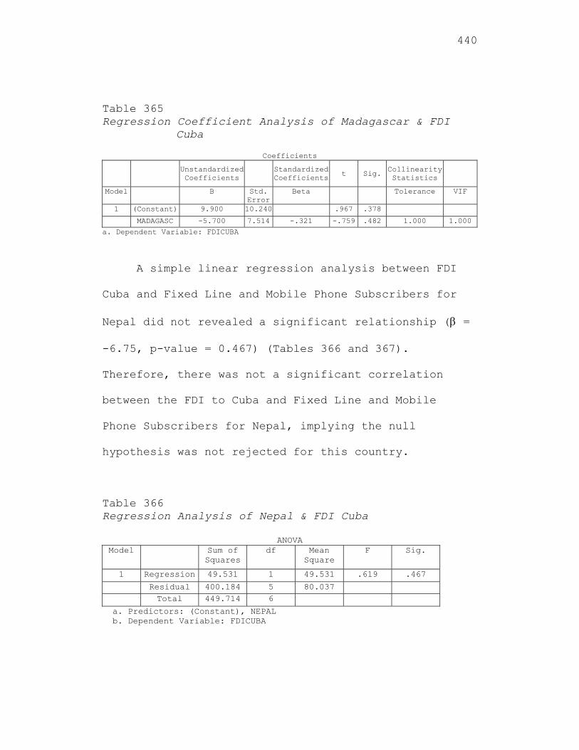
440

Table 365 Regression Coefficient Analysis of Madagascar & FDI

Cuba

Coefficients

Unstandardized Coefficients

Standardized Coefficients t Sig.

Collinearity Statistics

Model B Std. Error

Beta Tolerance VIF

1 (Constant) 9.900 10.240 .967 .378

MADAGASC -5.700 7.514 -.321 -.759 .482 1.000 1.000

a. Dependent Variable: FDICUBA

A simple linear regression analysis between FDI

Cuba and Fixed Line and Mobile Phone Subscribers for

Nepal did not revealed a significant relationship ( =

-6.75, p-value = 0.467) (Tables 366 and 367).

Therefore, there was not a significant correlation

between the FDI to Cuba and Fixed Line and Mobile

Phone Subscribers for Nepal, implying the null

hypothesis was not rejected for this country.

Table 366 Regression Analysis of Nepal & FDI Cuba

ANOVA Model Sum of

Squares df Mean

Square F Sig.

1 Regression 49.531 1 49.531 .619 .467

Residual 400.184 5 80.037 Total 449.714 6

a. Predictors: (Constant), NEPAL b. Dependent Variable: FDICUBA

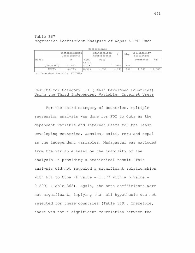
441

Table 367 Regression Coefficient Analysis of Nepal & FDI Cuba

Coefficients Unstandardized

Coefficients Standardized

Coefficientst Sig. Collinearity

Statistics

Model B Std. Error

Beta Tolerance VIF

1 (Constant) 12.593 13.181 .955 .383

NEPAL -6.745 8.575 -.332 -.787 .467 1.000 1.000

a. Dependent Variable: FDICUBA

Results for Category III (Least Developed Countries) Using the Third Independent Variable, Internet Users

For the third category of countries, multiple

regression analysis was done for FDI to Cuba as the

dependent variable and Internet Users for the least

Developing countries, Jamaica, Haiti, Peru and Nepal

as the independent variables. Madagascar was excluded

from the variable based on the inability of the

analysis in providing a statistical result. This

analysis did not revealed a significant relationships

with FDI to Cuba (F value = 1.677 with a p-value =

0.290) (Table 368). Again, the beta coefficients were

not significant, implying the null hypothesis was not

rejected for these countries (Table 369). Therefore,

there was not a significant correlation between the

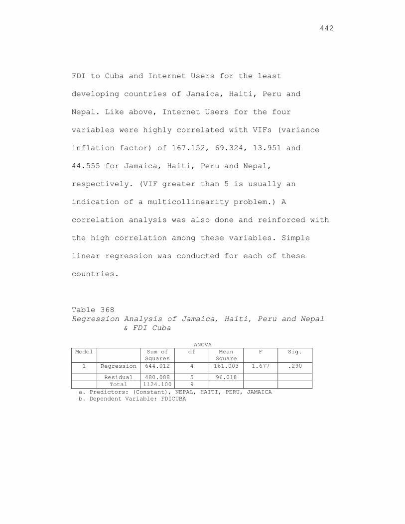
442

FDI to Cuba and Internet Users for the least

developing countries of Jamaica, Haiti, Peru and

Nepal. Like above, Internet Users for the four

variables were highly correlated with VIFs (variance

inflation factor) of 167.152, 69.324, 13.951 and

44.555 for Jamaica, Haiti, Peru and Nepal,

respectively. (VIF greater than 5 is usually an

indication of a multicollinearity problem.) A

correlation analysis was also done and reinforced with

the high correlation among these variables. Simple

linear regression was conducted for each of these

countries.

Table 368 Regression Analysis of Jamaica, Haiti, Peru and Nepal

& FDI Cuba

ANOVA Model Sum of

Squares df Mean

Square F Sig.

1 Regression 644.012 4 161.003 1.677 .290

Residual 480.088 5 96.018 Total 1124.100 9

a. Predictors: (Constant), NEPAL, HAITI, PERU, JAMAICA b. Dependent Variable: FDICUBA

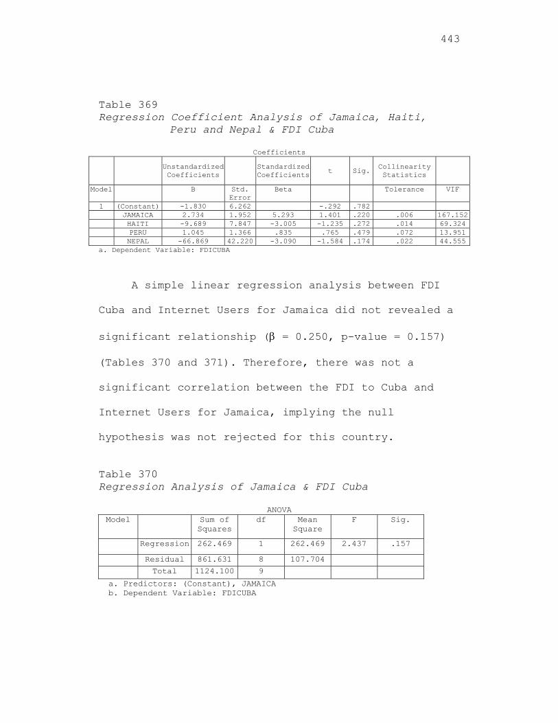
443

Table 369 Regression Coefficient Analysis of Jamaica, Haiti,

Peru and Nepal & FDI Cuba

Coefficients

Unstandardized Coefficients

Standardized Coefficients t Sig.

Collinearity Statistics

Model B Std. Error

Beta Tolerance VIF

1 (Constant) -1.830 6.262 -.292 .782 JAMAICA 2.734 1.952 5.293 1.401 .220 .006 167.152 HAITI -9.689 7.847 -3.005 -1.235 .272 .014 69.324 PERU 1.045 1.366 .835 .765 .479 .072 13.951 NEPAL -66.869 42.220 -3.090 -1.584 .174 .022 44.555a. Dependent Variable: FDICUBA

A simple linear regression analysis between FDI

Cuba and Internet Users for Jamaica did not revealed a

significant relationship ( = 0.250, p-value = 0.157)

(Tables 370 and 371). Therefore, there was not a

significant correlation between the FDI to Cuba and

Internet Users for Jamaica, implying the null

hypothesis was not rejected for this country.

Table 370 Regression Analysis of Jamaica & FDI Cuba

ANOVA Model Sum of

Squares df Mean

Square F Sig.

Regression 262.469 1 262.469 2.437 .157

Residual 861.631 8 107.704

Total 1124.100 9

a. Predictors: (Constant), JAMAICA b. Dependent Variable: FDICUBA

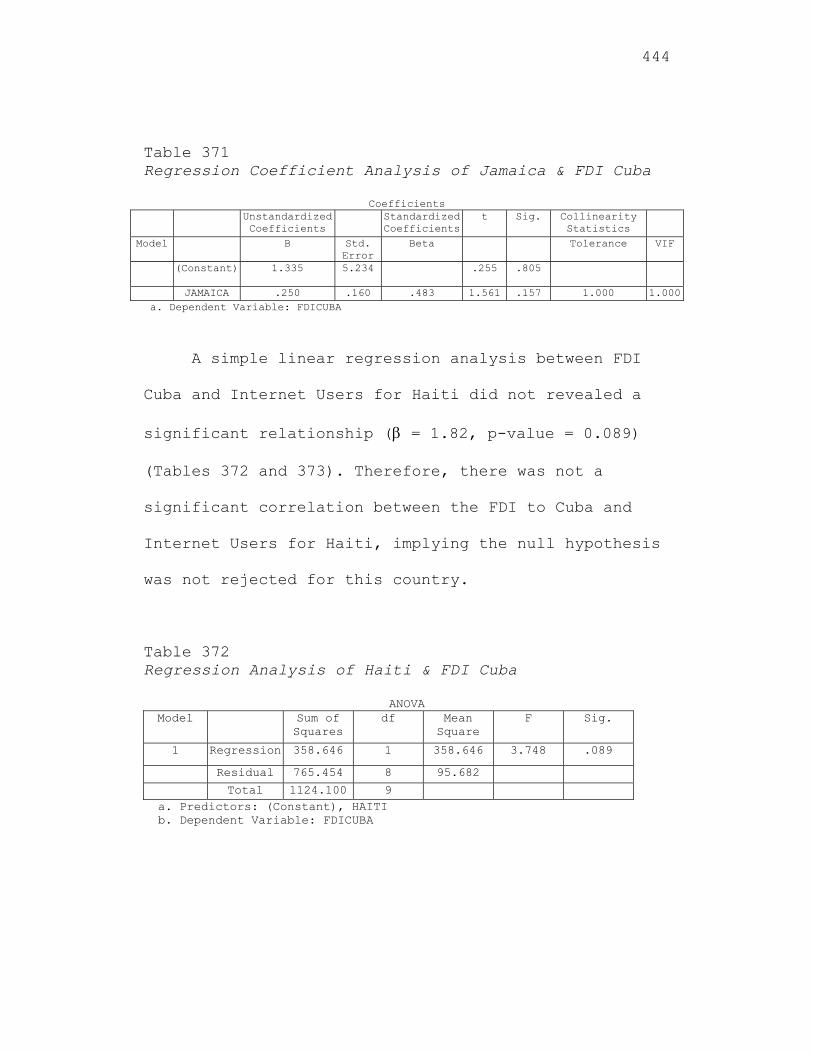
444

Table 371 Regression Coefficient Analysis of Jamaica & FDI Cuba

Coefficients Unstandardized

Coefficients Standardized

Coefficientst Sig. Collinearity

Statistics

Model B Std. Error

Beta Tolerance VIF

(Constant) 1.335 5.234 .255 .805

JAMAICA .250 .160 .483 1.561 .157 1.000 1.000 a. Dependent Variable: FDICUBA

A simple linear regression analysis between FDI

Cuba and Internet Users for Haiti did not revealed a

significant relationship ( = 1.82, p-value = 0.089)

(Tables 372 and 373). Therefore, there was not a

significant correlation between the FDI to Cuba and

Internet Users for Haiti, implying the null hypothesis

was not rejected for this country.

Table 372 Regression Analysis of Haiti & FDI Cuba

ANOVA Model Sum of

Squares df Mean

Square F Sig.

1 Regression 358.646 1 358.646 3.748 .089

Residual 765.454 8 95.682

Total 1124.100 9 a. Predictors: (Constant), HAITI b. Dependent Variable: FDICUBA

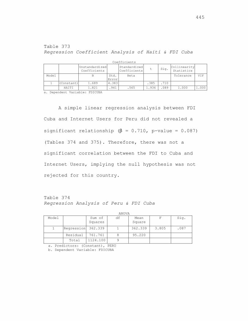
445

Table 373 Regression Coefficient Analysis of Haiti & FDI Cuba

Coefficients Unstandardized

Coefficients Standardized Coefficients t Sig.

Collinearity Statistics

Model B Std. Error

Beta Tolerance VIF

1 (Constant) 1.689 4.383 .385 .710 HAITI 1.821 .941 .565 1.936 .089 1.000 1.000

a. Dependent Variable: FDICUBA

A simple linear regression analysis between FDI

Cuba and Internet Users for Peru did not revealed a

significant relationship ( = 0.710, p-value = 0.087)

(Tables 374 and 375). Therefore, there was not a

significant correlation between the FDI to Cuba and

Internet Users, implying the null hypothesis was not

rejected for this country.

Table 374 Regression Analysis of Peru & FDI Cuba

ANOVA Model Sum of

Squares df Mean

Square F Sig.

1 Regression 362.339 1 362.339 3.805 .087

Residual 761.761 8 95.220 Total 1124.100 9

a. Predictors: (Constant), PERU b. Dependent Variable: FDICUBA

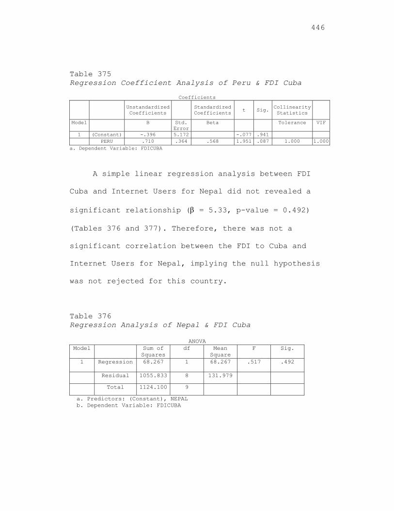
446

Table 375 Regression Coefficient Analysis of Peru & FDI Cuba

Coefficients

Unstandardized Coefficients

Standardized Coefficients

t Sig. Collinearity Statistics

Model B Std. Error

Beta Tolerance VIF

1 (Constant) -.396 5.172 -.077 .941 PERU .710 .364 .568 1.951 .087 1.000 1.000

a. Dependent Variable: FDICUBA

A simple linear regression analysis between FDI

Cuba and Internet Users for Nepal did not revealed a

significant relationship ( = 5.33, p-value = 0.492)

(Tables 376 and 377). Therefore, there was not a

significant correlation between the FDI to Cuba and

Internet Users for Nepal, implying the null hypothesis

was not rejected for this country.

Table 376 Regression Analysis of Nepal & FDI Cuba

ANOVA Model Sum of

Squares df Mean

Square F Sig.

1 Regression 68.267 1 68.267 .517 .492

Residual 1055.833 8 131.979

Total 1124.100 9

a. Predictors: (Constant), NEPAL b. Dependent Variable: FDICUBA

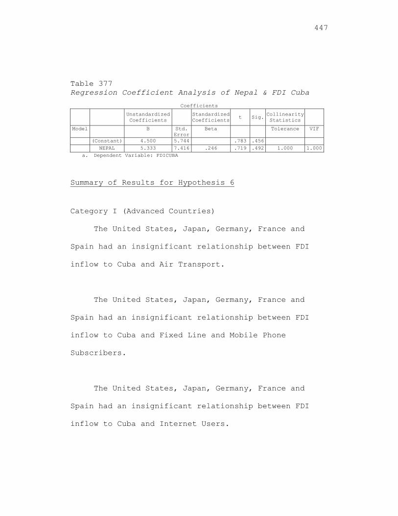
447

Table 377 Regression Coefficient Analysis of Nepal & FDI Cuba

Coefficients

Unstandardized Coefficients

Standardized Coefficients

t Sig. Collinearity Statistics

Model B Std. Error

Beta Tolerance VIF

(Constant) 4.500 5.744 .783 .456 NEPAL 5.333 7.416 .246 .719 .492 1.000 1.000a. Dependent Variable: FDICUBA

Summary of Results for Hypothesis 6

Category I (Advanced Countries)

The United States, Japan, Germany, France and

Spain had an insignificant relationship between FDI

inflow to Cuba and Air Transport.

The United States, Japan, Germany, France and

Spain had an insignificant relationship between FDI

inflow to Cuba and Fixed Line and Mobile Phone

Subscribers.

The United States, Japan, Germany, France and

Spain had an insignificant relationship between FDI

inflow to Cuba and Internet Users.

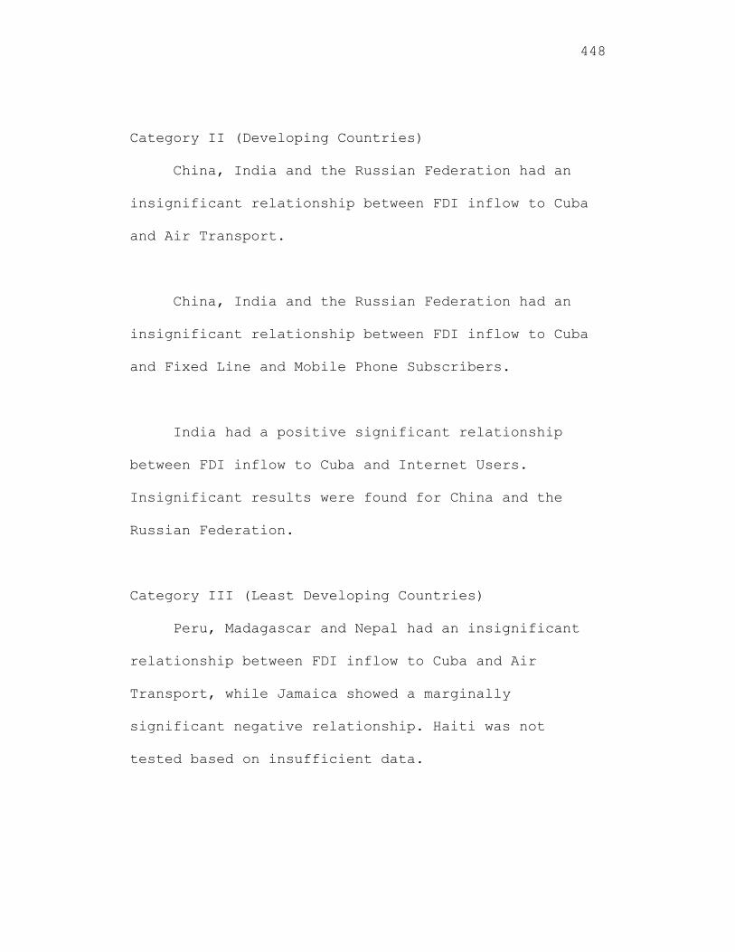
448

Category II (Developing Countries)

China, India and the Russian Federation had an

insignificant relationship between FDI inflow to Cuba

and Air Transport.

China, India and the Russian Federation had an

insignificant relationship between FDI inflow to Cuba

and Fixed Line and Mobile Phone Subscribers.

India had a positive significant relationship

between FDI inflow to Cuba and Internet Users.

Insignificant results were found for China and the

Russian Federation.

Category III (Least Developing Countries)

Peru, Madagascar and Nepal had an insignificant

relationship between FDI inflow to Cuba and Air

Transport, while Jamaica showed a marginally

significant negative relationship. Haiti was not

tested based on insufficient data.

449

Insignificant relationship existed between FDI

inflow to Cuba and Fixed Line and Mobile Phone

Subscribers for Jamaica, Haiti, Peru, Madagascar and

Nepal.

Insignificant relationship existed between FDI

inflow to Cuba and Internet Users for Jamaica, Haiti,

Peru and Nepal. Madagascar was not tested based on the

inability of the analysis in providing a statistical

result.

Results for Hypothesis 7

FDI to Cuba was the dependent variable. For the

advanced countries, the independent variables were

Market Type for the United States, Japan, Germany,

France and Spain (Sawalha, 2007). The independent

variables for the developing countries were Market

Type for China, India and the Russian Federation

(Sawalha, 2007). The independent variables for the

Least Developed Countries (LCD’s) were Market Type for

Jamaica, Haiti, Peru, Madagascar and Nepal. The

450

Republic of Cuba’s Market Type was not included in the

model as there were only three data points. The Market

Type included one variable, Merchandise Trade

(measured in percent of Gross Domestic Product).

The seventh hypothesis to be tested is:

Hypothesis H07: The level of contribution of

FDI inflow to Cuba is not significantly

related to the Market Type for the three

groups of countries.

Hypothesis HA7: The level of contribution of

FDI inflow to Cuba is significantly related to

the Market Type for the three groups of

countries.

The multiple regression models to test Hypothesis 7

are listed below.

Category I (Advanced Countries)

451

FDICUBA = αO + α1MARKETTYPEUS + α2MARKETTYPEJapan +

α3MARKETTYPEGermany + α4MARKETTYPEFrance +

α5MARKETTYPESpain + ε1

Categories II (Developing Countries)

FDICUBA = O + 1MARKETTYPEChina + 2MARKETTYPEIndia +

3MARKETTYPERussian Federation +ε2

Categories III (Least Developed Countries)

FDICUBA = δ + δ1MARKETTYPEJamaica + δ2MARKETTYPEHaiti +

δ3MARKETTYPEPeru + δ4MARKETTYPEMadagascar +

δ5MARKETTYPENepal + ε3

The results were presented for the independent

variables measuring Merchandise Trade for each of the

three categories of countries.

Pearson Correlation Analysis

A Pearson correlation analysis among the

advanced, developing and least developed of the 13 non

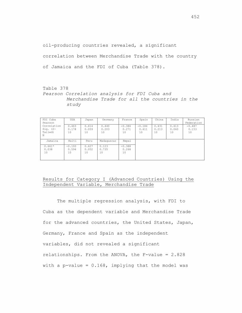
452

oil-producing countries revealed, a significant

correlation between Merchandise Trade with the country

of Jamaica and the FDI of Cuba (Table 378).

Table 378 Pearson Correlation analysis for FDI Cuba and

Merchandise Trade for all the countries in the study

FDI Cuba Pearson Correlation Sig. (2-Tailed) N

USA Japan Germany France Spain China India Russian Federation

0.463 0.178 10

0.614 0.059 10

0.440 0.203 10

-0.386 0.271 10

-0.184 0.611 10

0.431 0.213 10

0.613 0.060 10

-0.487 0.153 10

Jamaica Haiti Peru Madagascar Nepal

0.661* 0.038 10

-0.193 0.594 10

0.627 0.052 10

0.123 0.735 10

-0.388 0.268 10

Results for Category I (Advanced Countries) Using the Independent Variable, Merchandise Trade

The multiple regression analysis, with FDI to

Cuba as the dependent variable and Merchandise Trade

for the advanced countries, the United States, Japan,

Germany, France and Spain as the independent

variables, did not revealed a significant

relationships. From the ANOVA, the F-value = 2.828

with a p-value = 0.168, implying that the model was

453

not significant (Table 379). This was also observed

from the multiple regression analysis where the beta

coefficients were not significant, implying the null

hypothesis was not rejected for these countries (Table

380). Therefore, there was not a significant

correlation between the FDI to Cuba and Merchandise

Trade for these advanced countries, the United States,

Japan, Germany, France and Spain. This result was

surprising as France and Spain had been providing

significant FDI to Cuba (Travieso-Diaz & Trumbull,

2003). From the collinearity diagnostics, the variance

inflation factors (VIF) were 14.165, 148.201, 95.496,

14.892 and 9.517 for the United States, Japan,

Germany, France and Spain, respectively, implying a

major multicollinearity problem. (A VIF greater than 5

is usually an indication of a multicollinearity

problem.) This implies that the five independent

variables are highly correlated and cannot be utilized

for multiple regression analysis. A correlation

analysis further reinforced this position. Simple

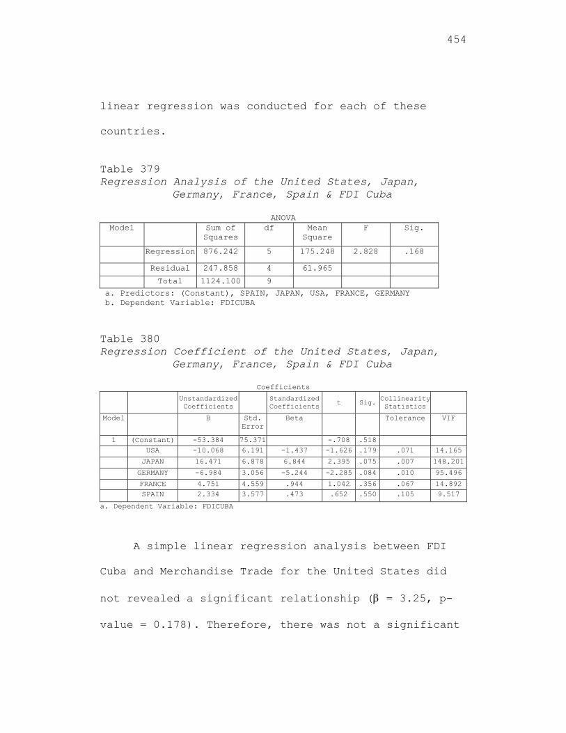
454

linear regression was conducted for each of these

countries.

Table 379 Regression Analysis of the United States, Japan,

Germany, France, Spain & FDI Cuba

ANOVA Model Sum of

Squares df Mean

Square F Sig.

Regression 876.242 5 175.248 2.828 .168

Residual 247.858 4 61.965

Total 1124.100 9

a. Predictors: (Constant), SPAIN, JAPAN, USA, FRANCE, GERMANY b. Dependent Variable: FDICUBA

Table 380 Regression Coefficient of the United States, Japan,

Germany, France, Spain & FDI Cuba

Coefficients Unstandardized

Coefficients

Standardized Coefficients

t Sig.Collinearity Statistics

Model B Std. Error

Beta Tolerance VIF

1 (Constant) -53.384 75.371 -.708 .518 USA -10.068 6.191 -1.437 -1.626 .179 .071 14.165

JAPAN 16.471 6.878 6.844 2.395 .075 .007 148.201

GERMANY -6.984 3.056 -5.244 -2.285 .084 .010 95.496

FRANCE 4.751 4.559 .944 1.042 .356 .067 14.892 SPAIN 2.334 3.577 .473 .652 .550 .105 9.517

a. Dependent Variable: FDICUBA

A simple linear regression analysis between FDI

Cuba and Merchandise Trade for the United States did

not revealed a significant relationship ( = 3.25, p-

value = 0.178). Therefore, there was not a significant

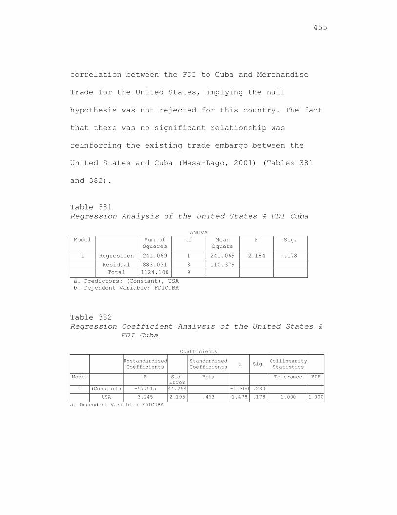
455

correlation between the FDI to Cuba and Merchandise

Trade for the United States, implying the null

hypothesis was not rejected for this country. The fact

that there was no significant relationship was

reinforcing the existing trade embargo between the

United States and Cuba (Mesa-Lago, 2001) (Tables 381

and 382).

Table 381 Regression Analysis of the United States & FDI Cuba

ANOVA Model Sum of

Squares df Mean

Square F Sig.

1 Regression 241.069 1 241.069 2.184 .178

Residual 883.031 8 110.379 Total 1124.100 9

a. Predictors: (Constant), USA b. Dependent Variable: FDICUBA Table 382 Regression Coefficient Analysis of the United States &

FDI Cuba

Coefficients

Unstandardized Coefficients

Standardized Coefficients

t Sig. Collinearity Statistics

Model B Std. Error

Beta Tolerance VIF

1 (Constant) -57.515 44.254 -1.300 .230

USA 3.245 2.195 .463 1.478 .178 1.000 1.000

a. Dependent Variable: FDICUBA

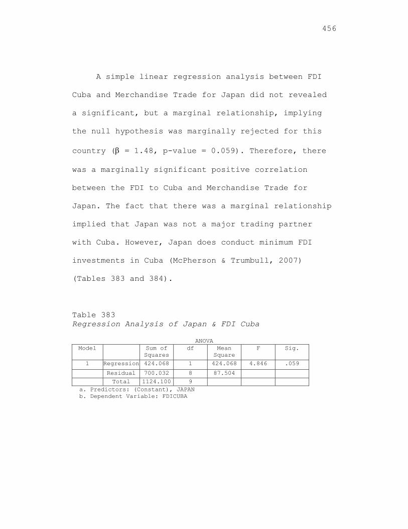
456

A simple linear regression analysis between FDI

Cuba and Merchandise Trade for Japan did not revealed

a significant, but a marginal relationship, implying

the null hypothesis was marginally rejected for this

country ( = 1.48, p-value = 0.059). Therefore, there

was a marginally significant positive correlation

between the FDI to Cuba and Merchandise Trade for

Japan. The fact that there was a marginal relationship

implied that Japan was not a major trading partner

with Cuba. However, Japan does conduct minimum FDI

investments in Cuba (McPherson & Trumbull, 2007)

(Tables 383 and 384).

Table 383 Regression Analysis of Japan & FDI Cuba

ANOVA Model Sum of

Squares df Mean

Square F Sig.

1 Regression 424.068 1 424.068 4.846 .059

Residual 700.032 8 87.504 Total 1124.100 9

a. Predictors: (Constant), JAPAN b. Dependent Variable: FDICUBA

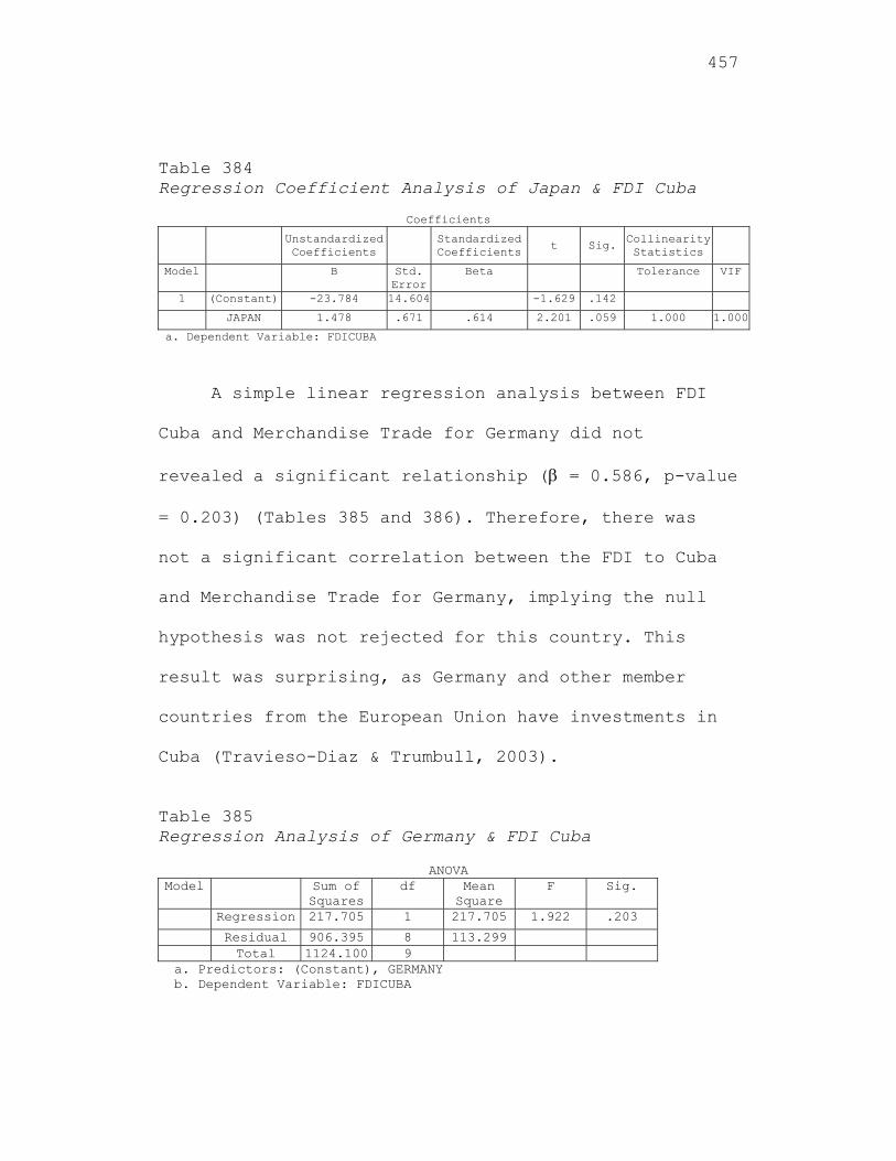
457

Table 384 Regression Coefficient Analysis of Japan & FDI Cuba

Coefficients Unstandardized

Coefficients Standardized

Coefficientst Sig. Collinearity

Statistics

Model B Std. Error

Beta Tolerance VIF

1 (Constant) -23.784 14.604 -1.629 .142

JAPAN 1.478 .671 .614 2.201 .059 1.000 1.000

a. Dependent Variable: FDICUBA

A simple linear regression analysis between FDI

Cuba and Merchandise Trade for Germany did not

revealed a significant relationship ( = 0.586, p-value

= 0.203) (Tables 385 and 386). Therefore, there was

not a significant correlation between the FDI to Cuba

and Merchandise Trade for Germany, implying the null

hypothesis was not rejected for this country. This

result was surprising, as Germany and other member

countries from the European Union have investments in

Cuba (Travieso-Diaz & Trumbull, 2003).

Table 385 Regression Analysis of Germany & FDI Cuba

ANOVA Model Sum of

Squaresdf Mean

Square F Sig.

Regression 217.705 1 217.705 1.922 .203

Residual 906.395 8 113.299 Total 1124.100 9

a. Predictors: (Constant), GERMANY b. Dependent Variable: FDICUBA

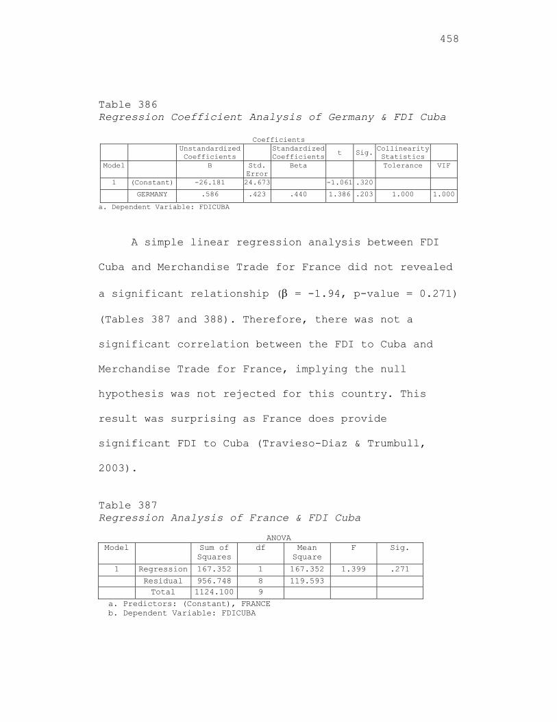
458

Table 386 Regression Coefficient Analysis of Germany & FDI Cuba

Coefficients Unstandardized

Coefficients Standardized

Coefficientst Sig. Collinearity

Statistics

Model B Std. Error

Beta Tolerance VIF

1 (Constant) -26.181 24.673 -1.061 .320

GERMANY .586 .423 .440 1.386 .203 1.000 1.000

a. Dependent Variable: FDICUBA

A simple linear regression analysis between FDI

Cuba and Merchandise Trade for France did not revealed

a significant relationship ( = -1.94, p-value = 0.271)

(Tables 387 and 388). Therefore, there was not a

significant correlation between the FDI to Cuba and

Merchandise Trade for France, implying the null

hypothesis was not rejected for this country. This

result was surprising as France does provide

significant FDI to Cuba (Travieso-Diaz & Trumbull,

2003).

Table 387 Regression Analysis of France & FDI Cuba

ANOVA

Model Sum of Squares

df Mean Square

F Sig.

1 Regression 167.352 1 167.352 1.399 .271

Residual 956.748 8 119.593 Total 1124.100 9

a. Predictors: (Constant), FRANCE b. Dependent Variable: FDICUBA

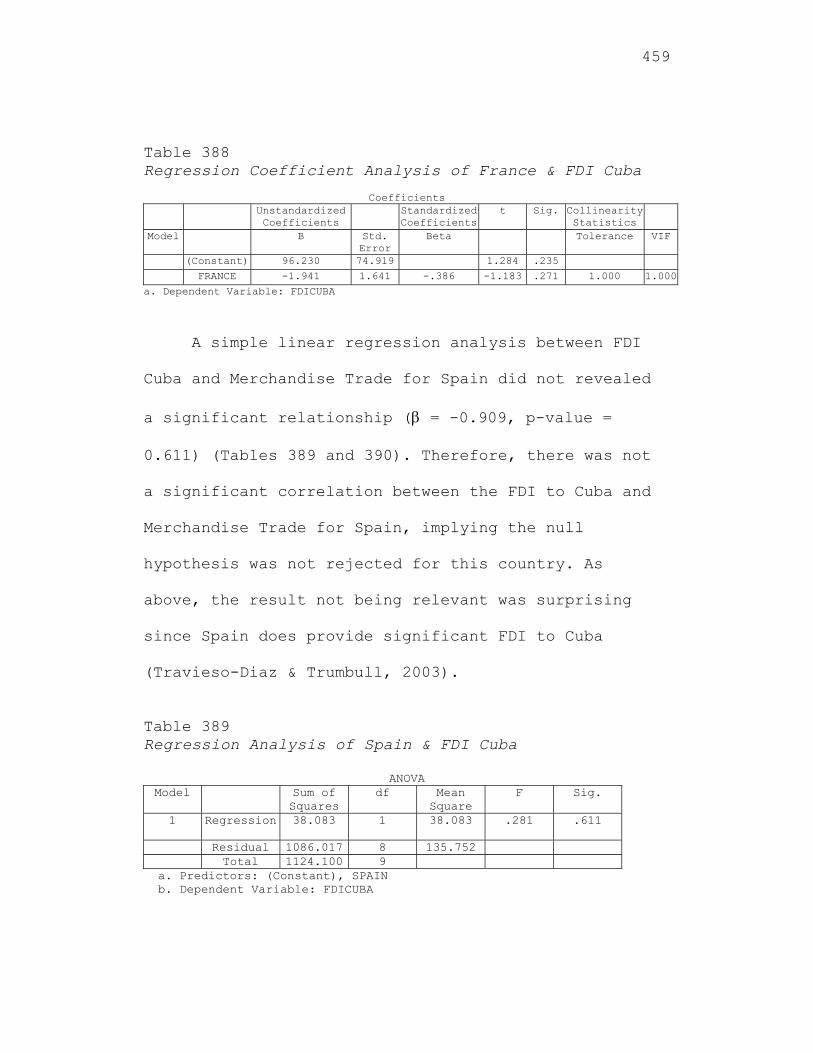
459

Table 388 Regression Coefficient Analysis of France & FDI Cuba

Coefficients

Unstandardized Coefficients

Standardized Coefficients

t Sig. Collinearity Statistics

Model B Std. Error

Beta Tolerance VIF

(Constant) 96.230 74.919 1.284 .235

FRANCE -1.941 1.641 -.386 -1.183 .271 1.000 1.000

a. Dependent Variable: FDICUBA

A simple linear regression analysis between FDI

Cuba and Merchandise Trade for Spain did not revealed

a significant relationship ( = -0.909, p-value =

0.611) (Tables 389 and 390). Therefore, there was not

a significant correlation between the FDI to Cuba and

Merchandise Trade for Spain, implying the null

hypothesis was not rejected for this country. As

above, the result not being relevant was surprising

since Spain does provide significant FDI to Cuba

(Travieso-Diaz & Trumbull, 2003).

Table 389 Regression Analysis of Spain & FDI Cuba

ANOVA Model Sum of

Squares df Mean

Square F Sig.

1 Regression 38.083 1 38.083 .281 .611

Residual 1086.017 8 135.752 Total 1124.100 9

a. Predictors: (Constant), SPAIN b. Dependent Variable: FDICUBA

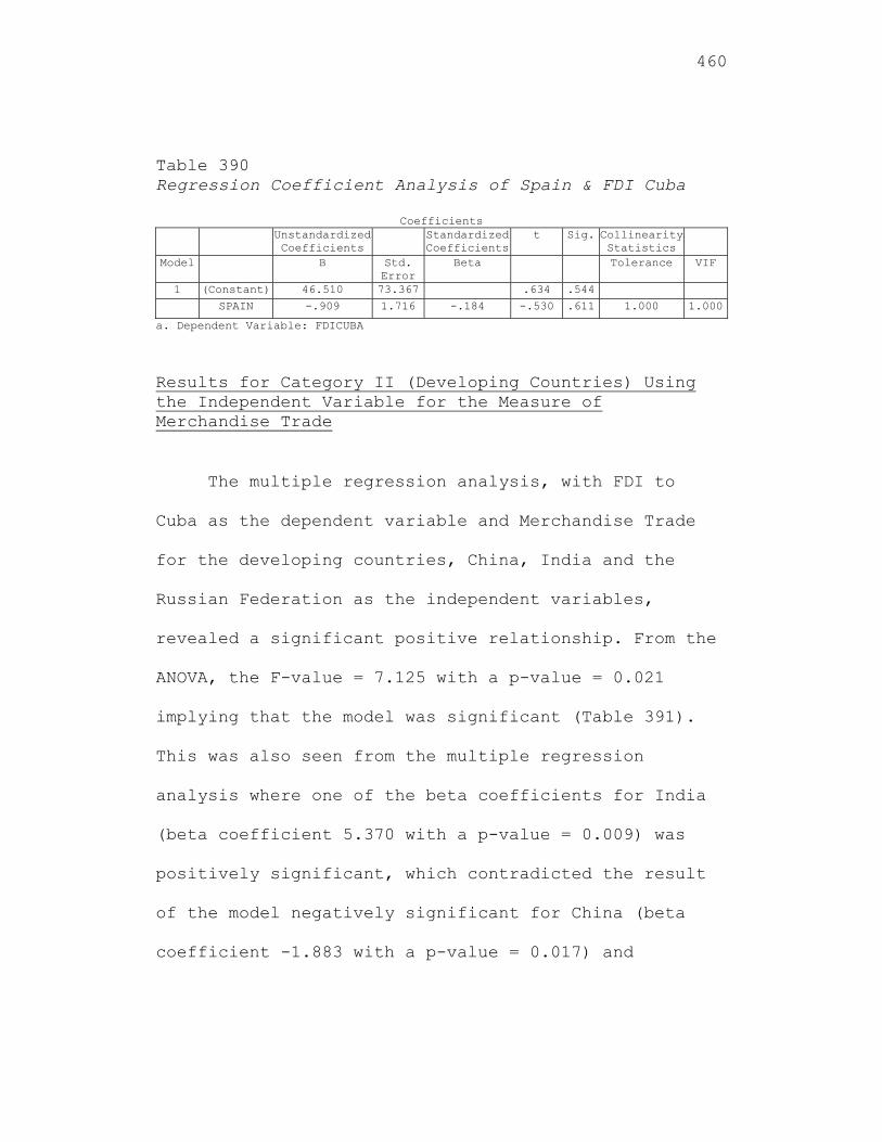
460

Table 390 Regression Coefficient Analysis of Spain & FDI Cuba

Coefficients Unstandardized

Coefficients Standardized

Coefficientst Sig. Collinearity

Statistics

Model B Std. Error

Beta Tolerance VIF

1 (Constant) 46.510 73.367 .634 .544

SPAIN -.909 1.716 -.184 -.530 .611 1.000 1.000

a. Dependent Variable: FDICUBA

Results for Category II (Developing Countries) Using the Independent Variable for the Measure of Merchandise Trade

The multiple regression analysis, with FDI to

Cuba as the dependent variable and Merchandise Trade

for the developing countries, China, India and the

Russian Federation as the independent variables,

revealed a significant positive relationship. From the

ANOVA, the F-value = 7.125 with a p-value = 0.021

implying that the model was significant (Table 391).

This was also seen from the multiple regression

analysis where one of the beta coefficients for India

(beta coefficient 5.370 with a p-value = 0.009) was

positively significant, which contradicted the result

of the model negatively significant for China (beta

coefficient -1.883 with a p-value = 0.017) and

461

insignificant for the Russian Federation (beta

coefficient -1.001 with a p-value = 0.174) (Table

392). Significant positive correlation between the FDI

to Cuba and Merchandise Trade for these developing

countries China, India and the Russian Federation

would imply that the null hypothesis was rejected for

these countries. From the collinearity diagnostics,

the variance inflation factors (VIF) were 14.272,

12.920 and 2.000 for China, India and the Russian

Federation, respectively, implying a major

multicollinearity problem. (As stated before a VIF

greater than 5 is usually an indication of a

multicollinearity problem.) This implied that two of

the three independent variables were highly correlated

and would not be utilized for multiple regression

analysis. A correlation analysis further reinforced

this position. Simple linear regression was conducted

for each of these countries.

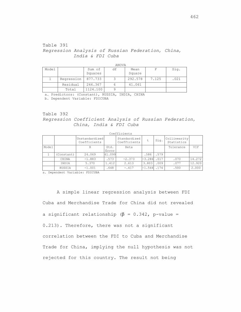
462

Table 391 Regression Analysis of Russian Federation, China,

India & FDI Cuba

ANOVA Model Sum of

Squares df Mean

Square F Sig.

1 Regression 877.733 3 292.578 7.125 .021

Residual 246.367 6 41.061 Total 1124.100 9

a. Predictors: (Constant), RUSSIA, INDIA, CHINA b. Dependent Variable: FDICUBA

Table 392 Regression Coefficient Analysis of Russian Federation,

China, India & FDI Cuba

Coefficients Unstandardized

Coefficients Standardized

Coefficientst Sig. Collinearity

Statistics

Model B Std. Error

Beta Tolerance VIF

1 (Constant) 24.069 41.099 .586 .579

CHINA -1.883 .573 -2.373 -3.286 .017 .070 14.272 INDIA 5.370 1.412 2.613 3.803 .009 .077 12.920

RUSSIA -1.001 .648 -.417 -1.544 .174 .500 2.000

a. Dependent Variable: FDICUBA

A simple linear regression analysis between FDI

Cuba and Merchandise Trade for China did not revealed

a significant relationship ( = 0.342, p-value =

0.213). Therefore, there was not a significant

correlation between the FDI to Cuba and Merchandise

Trade for China, implying the null hypothesis was not

rejected for this country. The result not being

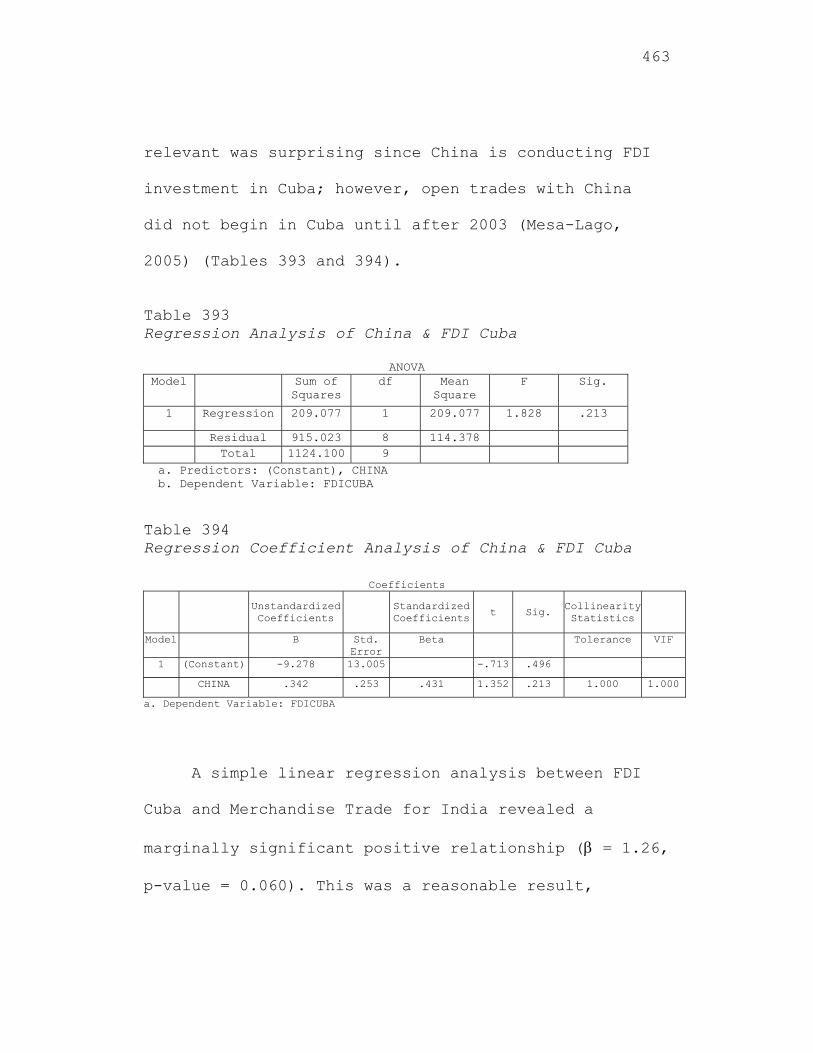
463

relevant was surprising since China is conducting FDI

investment in Cuba; however, open trades with China

did not begin in Cuba until after 2003 (Mesa-Lago,

2005) (Tables 393 and 394).

Table 393 Regression Analysis of China & FDI Cuba

ANOVA Model Sum of

Squares df Mean

Square F Sig.

1 Regression 209.077 1 209.077 1.828 .213

Residual 915.023 8 114.378 Total 1124.100 9

a. Predictors: (Constant), CHINA b. Dependent Variable: FDICUBA Table 394 Regression Coefficient Analysis of China & FDI Cuba

Coefficients

Unstandardized Coefficients

Standardized Coefficients t Sig.

Collinearity Statistics

Model B Std. Error

Beta Tolerance VIF

1 (Constant) -9.278 13.005 -.713 .496

CHINA .342 .253 .431 1.352 .213 1.000 1.000

a. Dependent Variable: FDICUBA

A simple linear regression analysis between FDI

Cuba and Merchandise Trade for India revealed a

marginally significant positive relationship ( = 1.26,

p-value = 0.060). This was a reasonable result,

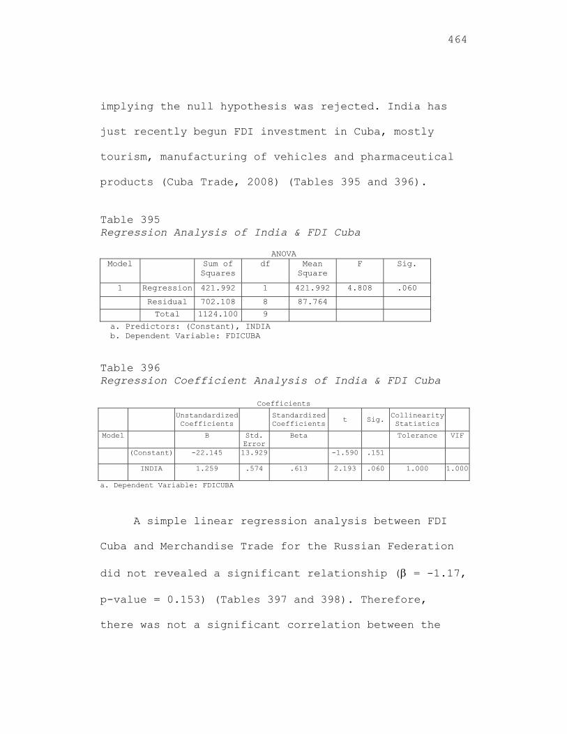
464

implying the null hypothesis was rejected. India has

just recently begun FDI investment in Cuba, mostly

tourism, manufacturing of vehicles and pharmaceutical

products (Cuba Trade, 2008) (Tables 395 and 396).

Table 395 Regression Analysis of India & FDI Cuba

ANOVA Model Sum of

Squares df Mean

Square F Sig.

1 Regression 421.992 1 421.992 4.808 .060

Residual 702.108 8 87.764

Total 1124.100 9

a. Predictors: (Constant), INDIA b. Dependent Variable: FDICUBA Table 396 Regression Coefficient Analysis of India & FDI Cuba

Coefficients Unstandardized

Coefficients

Standardized Coefficients

t Sig. Collinearity Statistics

Model B Std. Error

Beta Tolerance VIF

(Constant) -22.145 13.929 -1.590 .151

INDIA 1.259 .574 .613 2.193 .060 1.000 1.000

a. Dependent Variable: FDICUBA

A simple linear regression analysis between FDI

Cuba and Merchandise Trade for the Russian Federation

did not revealed a significant relationship ( = -1.17,

p-value = 0.153) (Tables 397 and 398). Therefore,

there was not a significant correlation between the

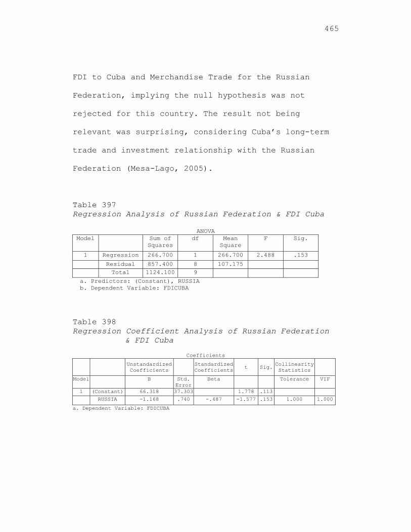
465

FDI to Cuba and Merchandise Trade for the Russian

Federation, implying the null hypothesis was not

rejected for this country. The result not being

relevant was surprising, considering Cuba’s long-term

trade and investment relationship with the Russian

Federation (Mesa-Lago, 2005).

Table 397 Regression Analysis of Russian Federation & FDI Cuba

ANOVA Model Sum of

Squares df Mean

Square F Sig.

1 Regression 266.700 1 266.700 2.488 .153

Residual 857.400 8 107.175 Total 1124.100 9

a. Predictors: (Constant), RUSSIA b. Dependent Variable: FDICUBA

Table 398 Regression Coefficient Analysis of Russian Federation

& FDI Cuba

Coefficients Unstandardized

Coefficients Standardized

Coefficientst Sig. Collinearity

Statistics

Model B Std. Error

Beta Tolerance VIF

1 (Constant) 66.318 37.303 1.778 .113

RUSSIA -1.168 .740 -.487 -1.577 .153 1.000 1.000

a. Dependent Variable: FDICUBA

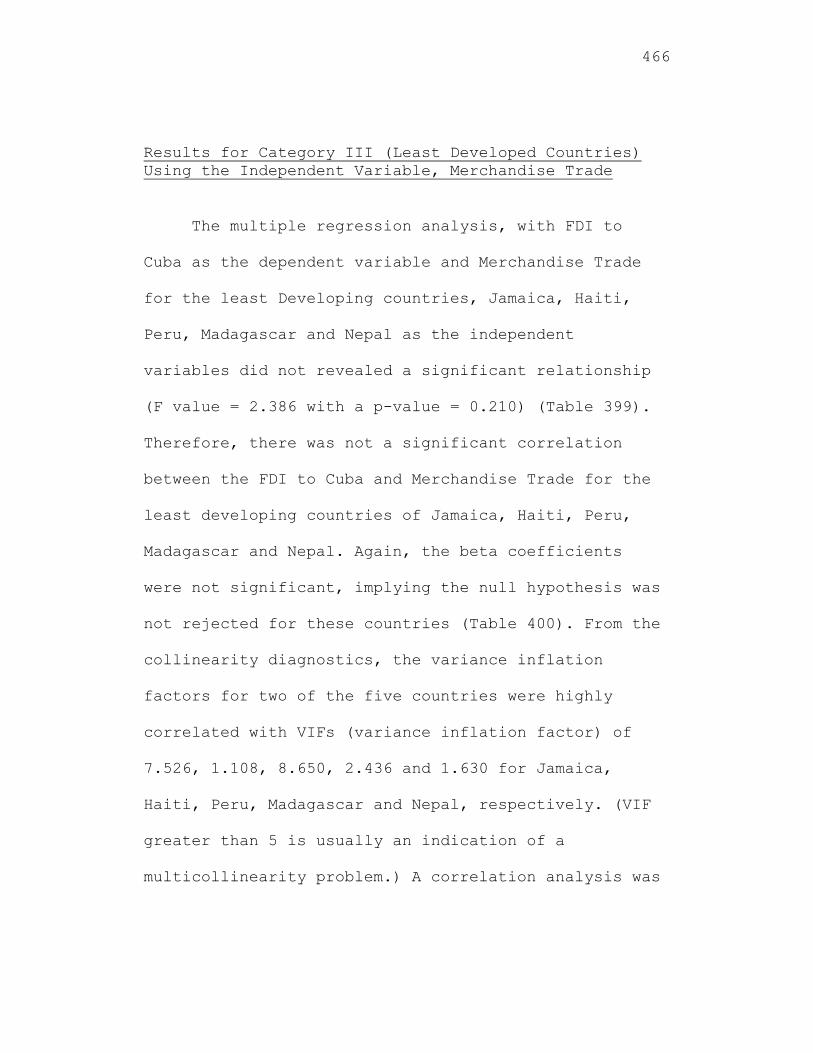
466

Results for Category III (Least Developed Countries) Using the Independent Variable, Merchandise Trade

The multiple regression analysis, with FDI to

Cuba as the dependent variable and Merchandise Trade

for the least Developing countries, Jamaica, Haiti,

Peru, Madagascar and Nepal as the independent

variables did not revealed a significant relationship

(F value = 2.386 with a p-value = 0.210) (Table 399).

Therefore, there was not a significant correlation

between the FDI to Cuba and Merchandise Trade for the

least developing countries of Jamaica, Haiti, Peru,

Madagascar and Nepal. Again, the beta coefficients

were not significant, implying the null hypothesis was

not rejected for these countries (Table 400). From the

collinearity diagnostics, the variance inflation

factors for two of the five countries were highly

correlated with VIFs (variance inflation factor) of

7.526, 1.108, 8.650, 2.436 and 1.630 for Jamaica,

Haiti, Peru, Madagascar and Nepal, respectively. (VIF

greater than 5 is usually an indication of a

multicollinearity problem.) A correlation analysis was

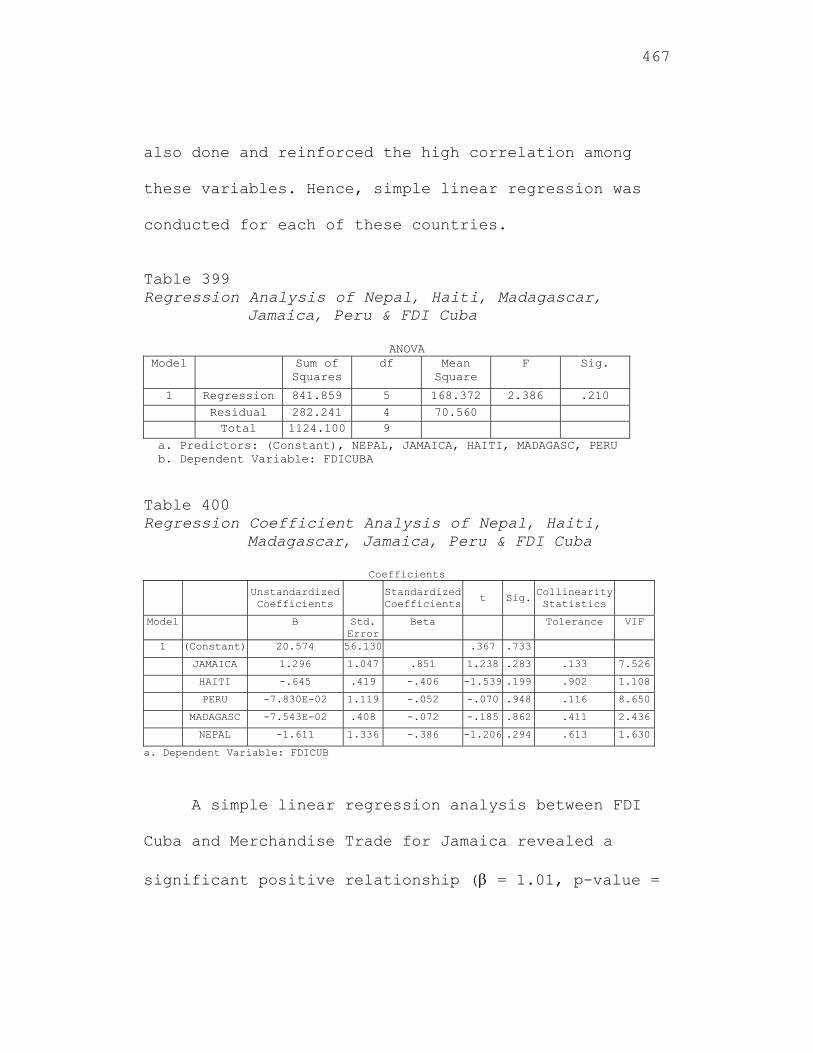
467

also done and reinforced the high correlation among

these variables. Hence, simple linear regression was

conducted for each of these countries.

Table 399 Regression Analysis of Nepal, Haiti, Madagascar,

Jamaica, Peru & FDI Cuba

ANOVA Model Sum of

Squares df Mean

Square F Sig.

1 Regression 841.859 5 168.372 2.386 .210 Residual 282.241 4 70.560 Total 1124.100 9

a. Predictors: (Constant), NEPAL, JAMAICA, HAITI, MADAGASC, PERU b. Dependent Variable: FDICUBA

Table 400 Regression Coefficient Analysis of Nepal, Haiti,

Madagascar, Jamaica, Peru & FDI Cuba

Coefficients Unstandardized

Coefficients Standardized

Coefficientst Sig. Collinearity

Statistics

Model B Std. Error

Beta Tolerance VIF

1 (Constant) 20.574 56.130 .367 .733

JAMAICA 1.296 1.047 .851 1.238 .283 .133 7.526

HAITI -.645 .419 -.406 -1.539 .199 .902 1.108

PERU -7.830E-02 1.119 -.052 -.070 .948 .116 8.650

MADAGASC -7.543E-02 .408 -.072 -.185 .862 .411 2.436

NEPAL -1.611 1.336 -.386 -1.206 .294 .613 1.630

a. Dependent Variable: FDICUB

A simple linear regression analysis between FDI

Cuba and Merchandise Trade for Jamaica revealed a

significant positive relationship ( = 1.01, p-value =

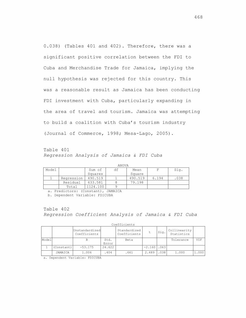
468

0.038) (Tables 401 and 402). Therefore, there was a

significant positive correlation between the FDI to

Cuba and Merchandise Trade for Jamaica, implying the

null hypothesis was rejected for this country. This

was a reasonable result as Jamaica has been conducting

FDI investment with Cuba, particularly expanding in

the area of travel and tourism. Jamaica was attempting

to build a coalition with Cuba’s tourism industry

(Journal of Commerce, 1998; Mesa-Lago, 2005).

Table 401 Regression Analysis of Jamaica & FDI Cuba

ANOVA Model Sum of

Squares df Mean

Square F Sig.

1 Regression 490.519 1 490.519 6.194 .038 Residual 633.581 8 79.198 Total 1124.100 9

a. Predictors: (Constant), JAMAICA b. Dependent Variable: FDICUBA Table 402 Regression Coefficient Analysis of Jamaica & FDI Cuba

Coefficients

Unstandardized Coefficients

Standardized Coefficients t Sig.

Collinearity Statistics

Model B Std. Error

Beta Tolerance VIF

1 (Constant) -53.175 24.622 -2.160 .063

JAMAICA 1.006 .404 .661 2.489 .038 1.000 1.000

a. Dependent Variable: FDICUBA

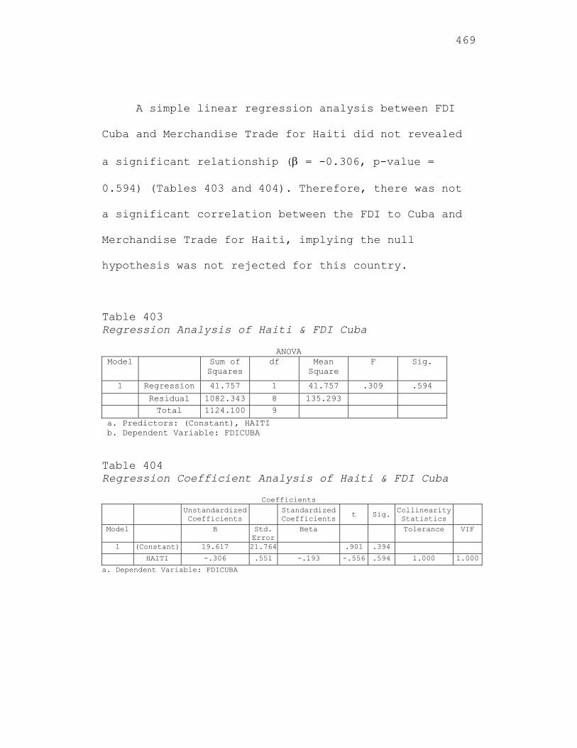
469

A simple linear regression analysis between FDI

Cuba and Merchandise Trade for Haiti did not revealed

a significant relationship ( = -0.306, p-value =

0.594) (Tables 403 and 404). Therefore, there was not

a significant correlation between the FDI to Cuba and

Merchandise Trade for Haiti, implying the null

hypothesis was not rejected for this country.

Table 403 Regression Analysis of Haiti & FDI Cuba

ANOVA Model Sum of

Squares df Mean

Square F Sig.

1 Regression 41.757 1 41.757 .309 .594

Residual 1082.343 8 135.293 Total 1124.100 9

a. Predictors: (Constant), HAITI b. Dependent Variable: FDICUBA Table 404 Regression Coefficient Analysis of Haiti & FDI Cuba

Coefficients Unstandardized

Coefficients Standardized

Coefficientst Sig. Collinearity

Statistics

Model B Std. Error

Beta Tolerance VIF

1 (Constant) 19.617 21.764 .901 .394

HAITI -.306 .551 -.193 -.556 .594 1.000 1.000

a. Dependent Variable: FDICUBA

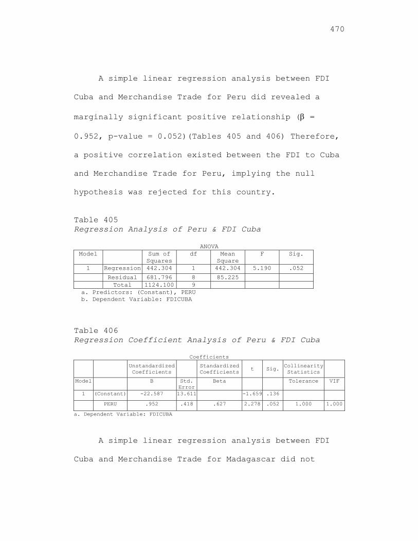
470

A simple linear regression analysis between FDI

Cuba and Merchandise Trade for Peru did revealed a

marginally significant positive relationship ( =

0.952, p-value = 0.052)(Tables 405 and 406) Therefore,

a positive correlation existed between the FDI to Cuba

and Merchandise Trade for Peru, implying the null

hypothesis was rejected for this country.

Table 405 Regression Analysis of Peru & FDI Cuba

ANOVA

Model Sum of Squares

df Mean Square

F Sig.

1 Regression 442.304 1 442.304 5.190 .052

Residual 681.796 8 85.225 Total 1124.100 9

a. Predictors: (Constant), PERU b. Dependent Variable: FDICUBA Table 406 Regression Coefficient Analysis of Peru & FDI Cuba

Coefficients Unstandardized

Coefficients Standardized

Coefficientst Sig. Collinearity

Statistics

Model B Std. Error

Beta Tolerance VIF

1 (Constant) -22.587 13.611 -1.659 .136

PERU .952 .418 .627 2.278 .052 1.000 1.000

a. Dependent Variable: FDICUBA

A simple linear regression analysis between FDI

Cuba and Merchandise Trade for Madagascar did not

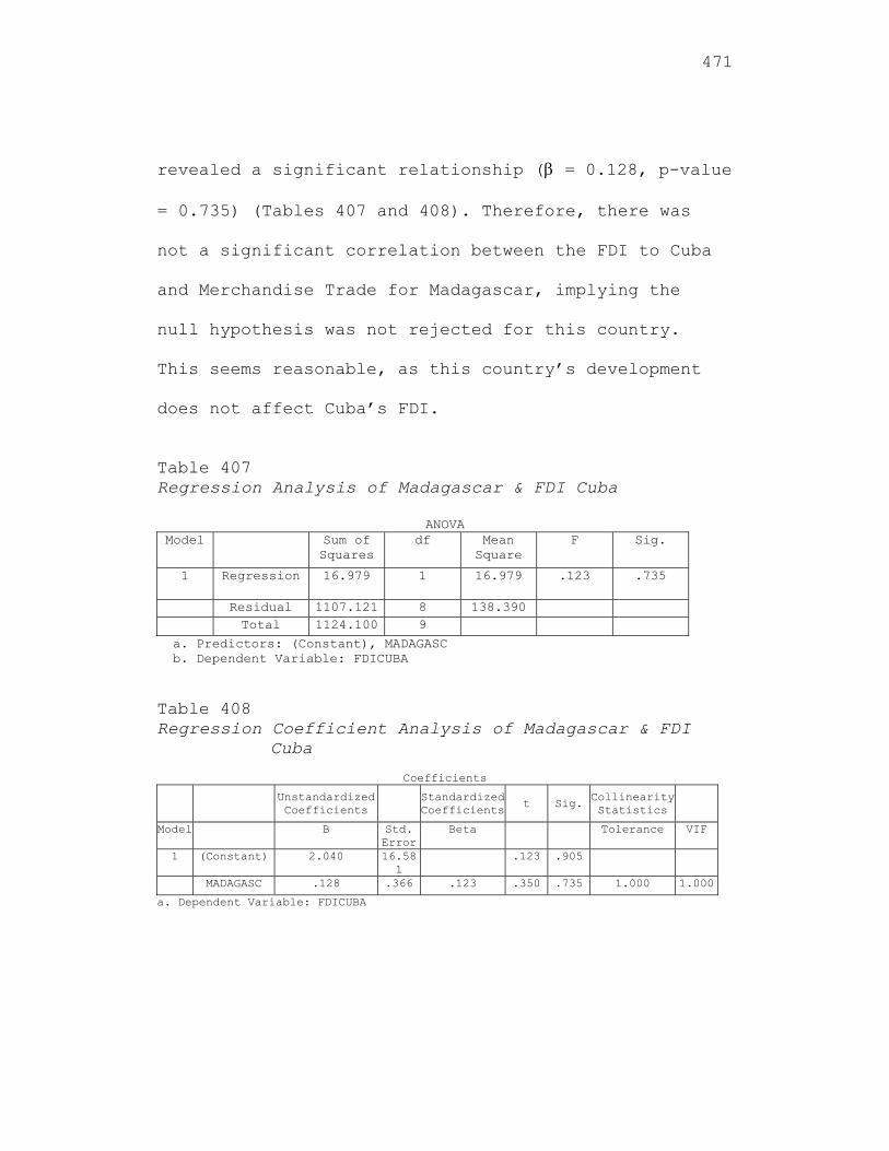
471

revealed a significant relationship ( = 0.128, p-value

= 0.735) (Tables 407 and 408). Therefore, there was

not a significant correlation between the FDI to Cuba

and Merchandise Trade for Madagascar, implying the

null hypothesis was not rejected for this country.

This seems reasonable, as this country’s development

does not affect Cuba’s FDI.

Table 407 Regression Analysis of Madagascar & FDI Cuba

ANOVA Model Sum of

Squares df Mean

Square F Sig.

1 Regression 16.979 1 16.979 .123 .735

Residual 1107.121 8 138.390 Total 1124.100 9

a. Predictors: (Constant), MADAGASC b. Dependent Variable: FDICUBA Table 408 Regression Coefficient Analysis of Madagascar & FDI

Cuba

Coefficients Unstandardized

Coefficients Standardized

Coefficientst Sig. Collinearity

Statistics

Model B Std. Error

Beta Tolerance VIF

1 (Constant) 2.040 16.581

.123 .905

MADAGASC .128 .366 .123 .350 .735 1.000 1.000

a. Dependent Variable: FDICUBA

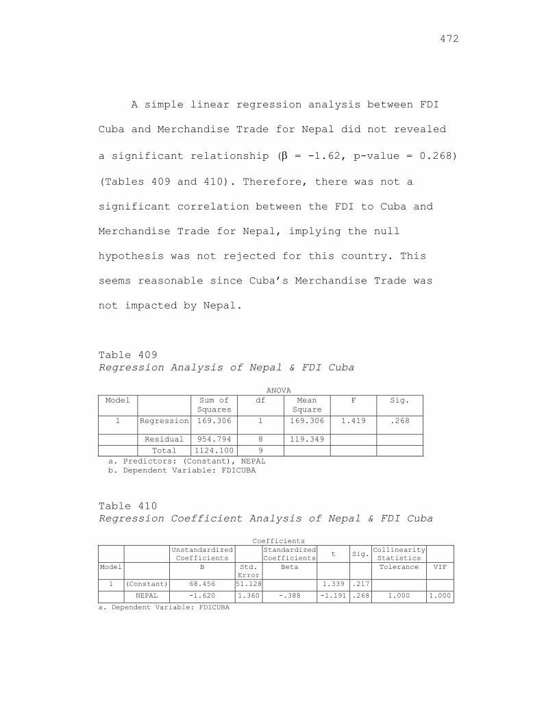
472

A simple linear regression analysis between FDI

Cuba and Merchandise Trade for Nepal did not revealed

a significant relationship ( = -1.62, p-value = 0.268)

(Tables 409 and 410). Therefore, there was not a

significant correlation between the FDI to Cuba and

Merchandise Trade for Nepal, implying the null

hypothesis was not rejected for this country. This

seems reasonable since Cuba’s Merchandise Trade was

not impacted by Nepal.

Table 409 Regression Analysis of Nepal & FDI Cuba

ANOVA Model Sum of

Squares df Mean

Square F Sig.

1 Regression 169.306 1 169.306 1.419 .268

Residual 954.794 8 119.349 Total 1124.100 9

a. Predictors: (Constant), NEPAL b. Dependent Variable: FDICUBA

Table 410 Regression Coefficient Analysis of Nepal & FDI Cuba

Coefficients Unstandardized

Coefficients Standardized

Coefficientst Sig. Collinearity

Statistics

Model B Std. Error

Beta Tolerance VIF

1 (Constant) 68.456 51.128 1.339 .217

NEPAL -1.620 1.360 -.388 -1.191 .268 1.000 1.000

a. Dependent Variable: FDICUBA

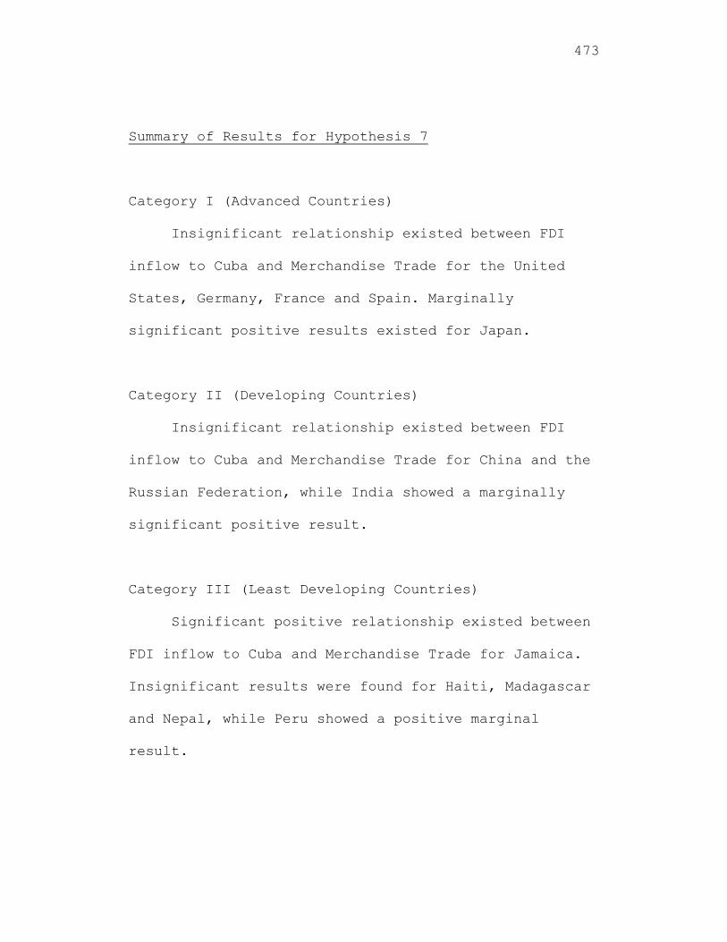
473

Summary of Results for Hypothesis 7

Category I (Advanced Countries)

Insignificant relationship existed between FDI

inflow to Cuba and Merchandise Trade for the United

States, Germany, France and Spain. Marginally

significant positive results existed for Japan.

Category II (Developing Countries)

Insignificant relationship existed between FDI

inflow to Cuba and Merchandise Trade for China and the

Russian Federation, while India showed a marginally

significant positive result.

Category III (Least Developing Countries)

Significant positive relationship existed between

FDI inflow to Cuba and Merchandise Trade for Jamaica.

Insignificant results were found for Haiti, Madagascar

and Nepal, while Peru showed a positive marginal

result.

474

Results for Hypothesis 8

FDI to Cuba was the dependent variable. For the

advanced countries, the independent variables were

Environment Factors for the United States, Japan,

Germany, France and Spain (Sawalha, 2007). The

independent variables for the developing countries

were Environment Factors for China, India and the

Russian Federation (Sawalha, 2007). The independent

variables for the Least Developed Countries (LCD’s)

were Environment Factors for Jamaica, Haiti, Peru,

Madagascar and Nepal. The Republic of Cuba’s

Environment Factors was not included in the model as

there were only three data points. The Environment

Factors included one variable, Agriculture value added

(measured in percent of Gross Domestic Product).

The eighth hypothesis to be tested is:

Hypothesis H08: The level of contribution of

FDI inflow to Cuba is not significantly

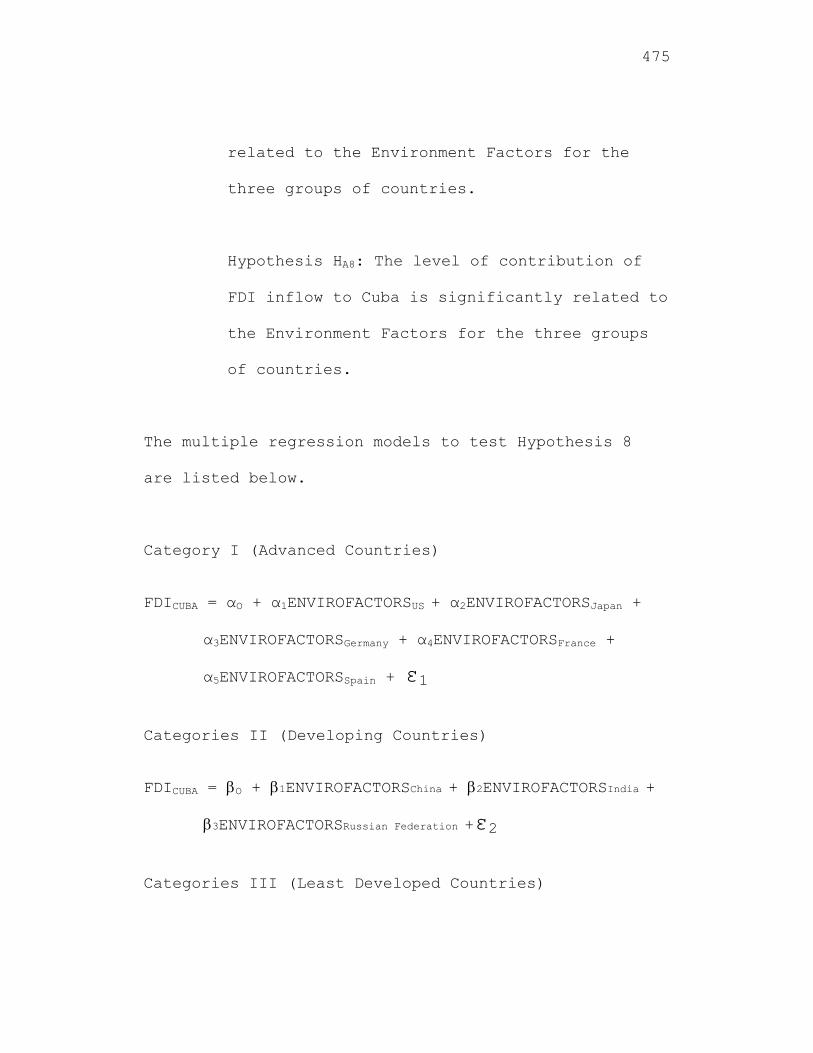
475

related to the Environment Factors for the

three groups of countries.

Hypothesis HA8: The level of contribution of

FDI inflow to Cuba is significantly related to

the Environment Factors for the three groups

of countries.

The multiple regression models to test Hypothesis 8

are listed below.

Category I (Advanced Countries)

FDICUBA = αO + α1ENVIROFACTORSUS + α2ENVIROFACTORSJapan +

α3ENVIROFACTORSGermany + α4ENVIROFACTORSFrance +

α5ENVIROFACTORSSpain + ε1

Categories II (Developing Countries)

FDICUBA = O + 1ENVIROFACTORSChina + 2ENVIROFACTORSIndia +

3ENVIROFACTORSRussian Federation +ε2

Categories III (Least Developed Countries)

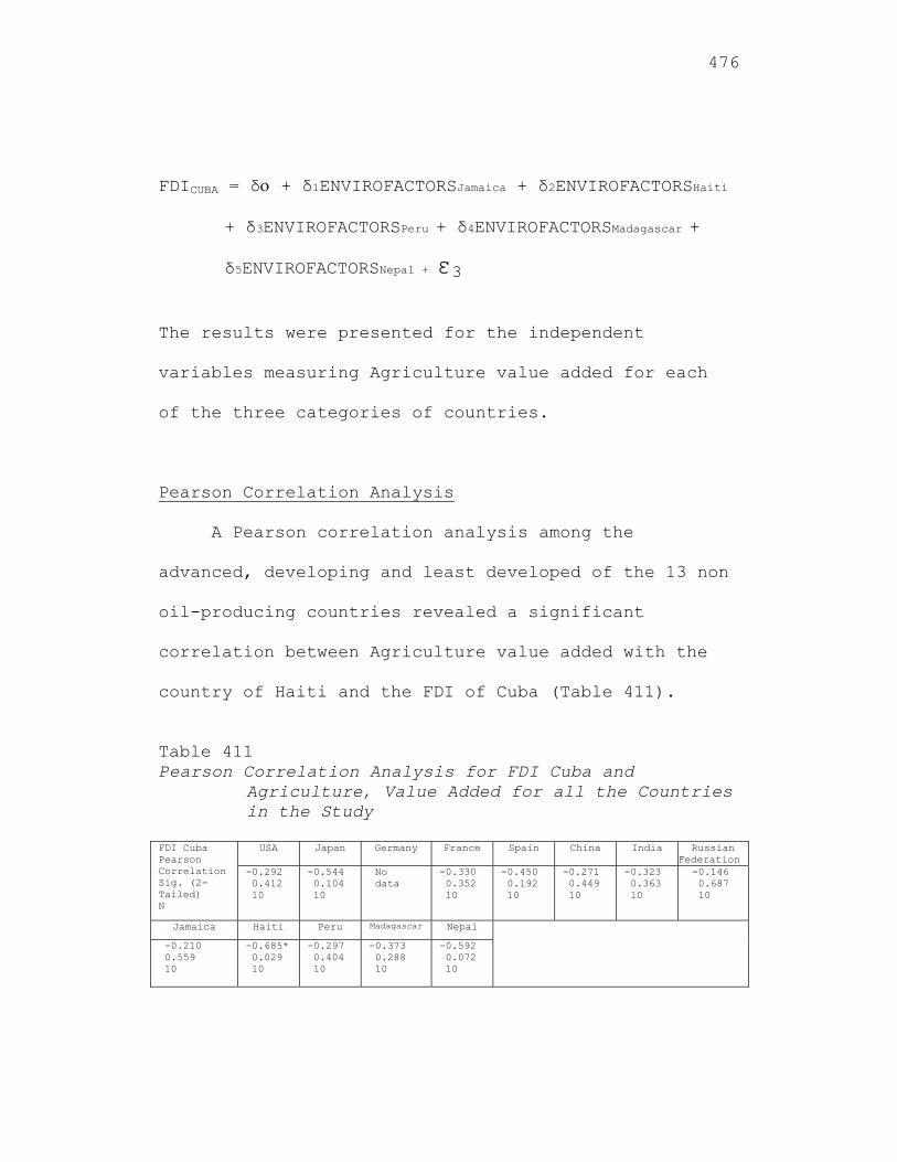
476

FDICUBA = δ + δ1ENVIROFACTORSJamaica + δ2ENVIROFACTORSHaiti

+ δ3ENVIROFACTORSPeru + δ4ENVIROFACTORSMadagascar +

δ5ENVIROFACTORSNepal + ε3

The results were presented for the independent

variables measuring Agriculture value added for each

of the three categories of countries.

Pearson Correlation Analysis

A Pearson correlation analysis among the

advanced, developing and least developed of the 13 non

oil-producing countries revealed a significant

correlation between Agriculture value added with the

country of Haiti and the FDI of Cuba (Table 411).

Table 411 Pearson Correlation Analysis for FDI Cuba and

Agriculture, Value Added for all the Countries in the Study

FDI Cuba Pearson Correlation Sig. (2-Tailed) N

USA Japan Germany France Spain China India Russian Federation

-0.292 0.412 10

-0.544 0.104 10

No data

-0.330 0.352 10

-0.450 0.192 10

-0.271 0.449 10

-0.323 0.363 10

-0.146 0.687 10

Jamaica Haiti Peru Madagascar Nepal

-0.210 0.559 10

-0.685* 0.029 10

-0.297 0.404 10

-0.373 0.288 10

-0.592 0.072 10

477

Results for Category I (Advanced Countries) Using the Independent Variable, Agriculture Value Added

The multiple regression analysis, with FDI to

Cuba as the dependent variable and Agriculture value

added for the advanced countries, the United States,

Japan, France and Spain as the independent variables,

did not revealed a significant relationships. Germany

was excluded from the analysis since the variable of

the data was constant and insignificant for testing.

From the ANOVA, the F-value = 1.065 with a p-value =

0.461, implying that the model was not significant

(Table 412). This was also seen from the multiple

regression analysis where the beta coefficients were

not significant, implying the null hypothesis was not

rejected for these countries (Table 413). Therefore,

there was not a significant correlation between the

FDI to Cuba and Agriculture value added for these

advanced countries, the United States, Japan, France

and Spain. From the collinearity diagnostics, the

variance inflation factors (VIF) were 5.073, 6.709,

1.818 and 2.455 for the United States, Japan, France

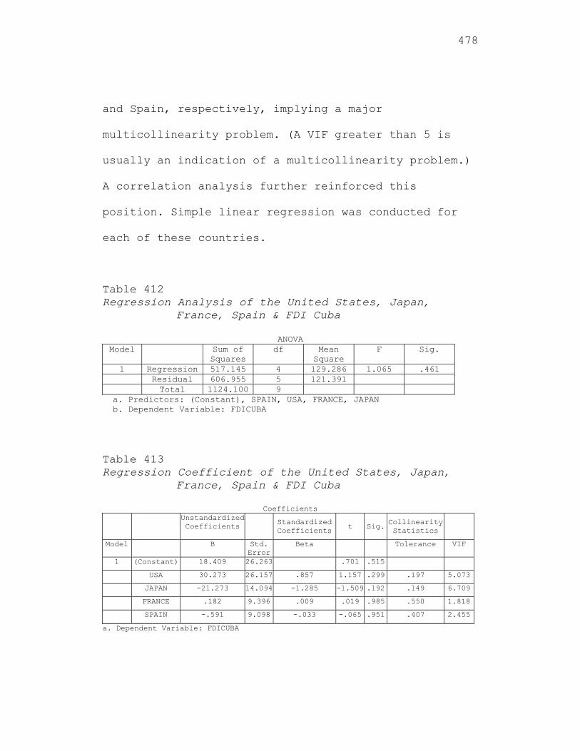
478

and Spain, respectively, implying a major

multicollinearity problem. (A VIF greater than 5 is

usually an indication of a multicollinearity problem.)

A correlation analysis further reinforced this

position. Simple linear regression was conducted for

each of these countries.

Table 412 Regression Analysis of the United States, Japan,

France, Spain & FDI Cuba

ANOVA Model Sum of

Squares df Mean

Square F Sig.

1 Regression 517.145 4 129.286 1.065 .461 Residual 606.955 5 121.391 Total 1124.100 9

a. Predictors: (Constant), SPAIN, USA, FRANCE, JAPAN b. Dependent Variable: FDICUBA

Table 413 Regression Coefficient of the United States, Japan,

France, Spain & FDI Cuba

Coefficients Unstandardized

Coefficients

Standardized Coefficients t Sig.

Collinearity Statistics

Model B Std. Error

Beta Tolerance VIF

1 (Constant) 18.409 26.263 .701 .515

USA 30.273 26.157 .857 1.157 .299 .197 5.073

JAPAN -21.273 14.094 -1.285 -1.509 .192 .149 6.709

FRANCE .182 9.396 .009 .019 .985 .550 1.818

SPAIN -.591 9.098 -.033 -.065 .951 .407 2.455

a. Dependent Variable: FDICUBA

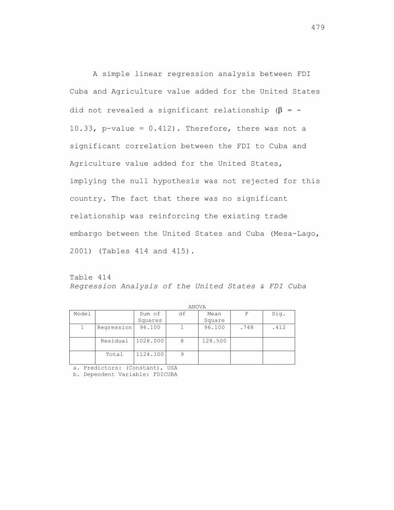
479

A simple linear regression analysis between FDI

Cuba and Agriculture value added for the United States

did not revealed a significant relationship ( = -

10.33, p-value = 0.412). Therefore, there was not a

significant correlation between the FDI to Cuba and

Agriculture value added for the United States,

implying the null hypothesis was not rejected for this

country. The fact that there was no significant

relationship was reinforcing the existing trade

embargo between the United States and Cuba (Mesa-Lago,

2001) (Tables 414 and 415).

Table 414 Regression Analysis of the United States & FDI Cuba

ANOVA Model Sum of

Squares df Mean

Square F Sig.

1

Regression 96.100 1 96.100 .748 .412

Residual 1028.000 8 128.500

Total 1124.100 9

a. Predictors: (Constant), USA b. Dependent Variable: FDICUBA

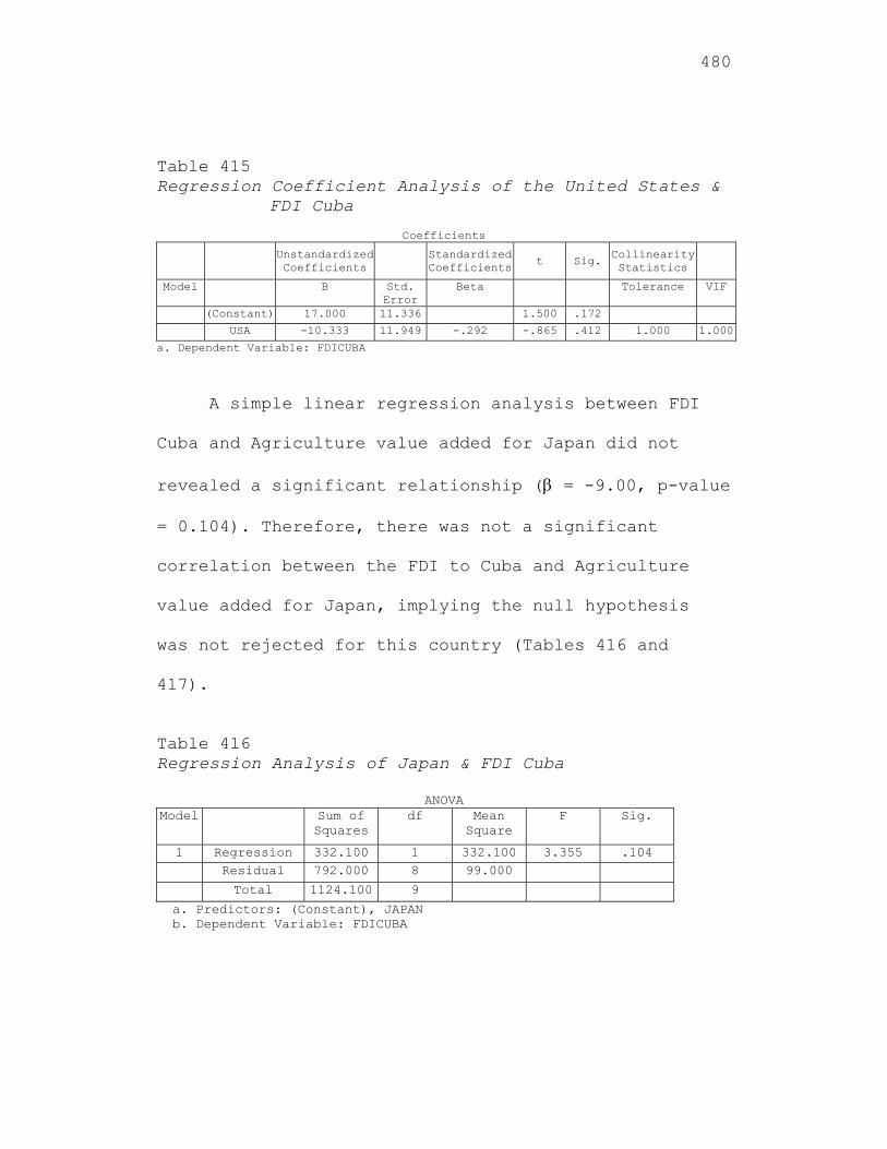
480

Table 415 Regression Coefficient Analysis of the United States &

FDI Cuba

Coefficients Unstandardized

Coefficients Standardized

Coefficientst Sig. Collinearity

Statistics

Model B Std. Error

Beta Tolerance VIF

(Constant) 17.000 11.336 1.500 .172

USA -10.333 11.949 -.292 -.865 .412 1.000 1.000

a. Dependent Variable: FDICUBA

A simple linear regression analysis between FDI

Cuba and Agriculture value added for Japan did not

revealed a significant relationship ( = -9.00, p-value

= 0.104). Therefore, there was not a significant

correlation between the FDI to Cuba and Agriculture

value added for Japan, implying the null hypothesis

was not rejected for this country (Tables 416 and

417).

Table 416 Regression Analysis of Japan & FDI Cuba

ANOVA Model Sum of

Squares df Mean

Square F Sig.

1 Regression 332.100 1 332.100 3.355 .104 Residual 792.000 8 99.000

Total 1124.100 9

a. Predictors: (Constant), JAPAN b. Dependent Variable: FDICUBA

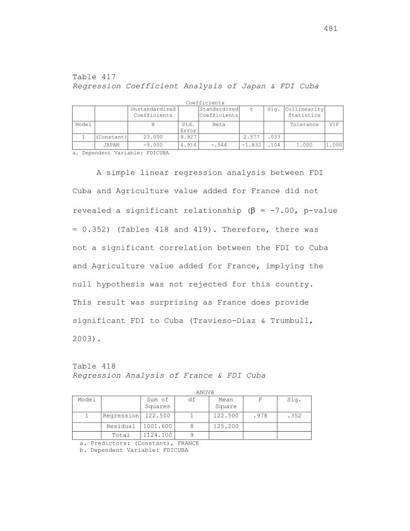
481

Table 417 Regression Coefficient Analysis of Japan & FDI Cuba

Coefficients Unstandardized

Coefficients Standardized

Coefficientst Sig. Collinearity

Statistics

Model B Std. Error

Beta Tolerance VIF

1 (Constant) 23.000 8.927 2.577 .033

JAPAN -9.000 4.914 -.544 -1.832 .104 1.000 1.000

a. Dependent Variable: FDICUBA

A simple linear regression analysis between FDI

Cuba and Agriculture value added for France did not

revealed a significant relationship ( = -7.00, p-value

= 0.352) (Tables 418 and 419). Therefore, there was

not a significant correlation between the FDI to Cuba

and Agriculture value added for France, implying the

null hypothesis was not rejected for this country.

This result was surprising as France does provide

significant FDI to Cuba (Travieso-Diaz & Trumbull,

2003).

Table 418 Regression Analysis of France & FDI Cuba

ANOVA Model Sum of

Squares df Mean

Square F Sig.

1 Regression 122.500 1 122.500 .978 .352

Residual 1001.600 8 125.200

Total 1124.100 9 a. Predictors: (Constant), FRANCE b. Dependent Variable: FDICUBA

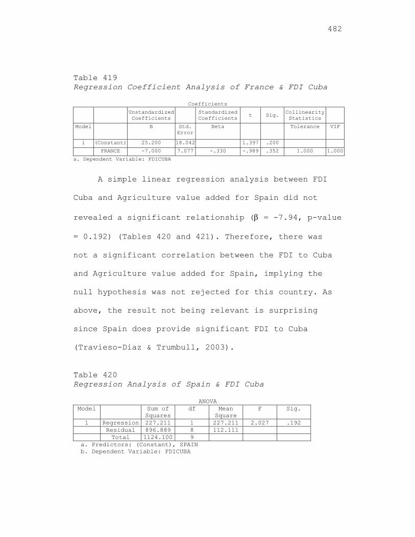
482

Table 419 Regression Coefficient Analysis of France & FDI Cuba

Coefficients Unstandardized

Coefficients Standardized Coefficients t Sig.

Collinearity Statistics

Model B Std. Error

Beta Tolerance VIF

1 (Constant) 25.200 18.042 1.397 .200

FRANCE -7.000 7.077 -.330 -.989 .352 1.000 1.000

a. Dependent Variable: FDICUBA

A simple linear regression analysis between FDI

Cuba and Agriculture value added for Spain did not

revealed a significant relationship ( = -7.94, p-value

= 0.192) (Tables 420 and 421). Therefore, there was

not a significant correlation between the FDI to Cuba

and Agriculture value added for Spain, implying the

null hypothesis was not rejected for this country. As

above, the result not being relevant is surprising

since Spain does provide significant FDI to Cuba

(Travieso-Diaz & Trumbull, 2003).

Table 420 Regression Analysis of Spain & FDI Cuba

ANOVA Model Sum of

Squares df Mean

Square F Sig.

1 Regression 227.211 1 227.211 2.027 .192 Residual 896.889 8 112.111 Total 1124.100 9

a. Predictors: (Constant), SPAIN b. Dependent Variable: FDICUBA

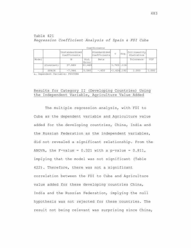
483

Table 421 Regression Coefficient Analysis of Spain & FDI Cuba

Coefficients

Unstandardized Coefficients

Standardized Coefficients

t Sig. Collinearity Statistics

Model B Std. Error

Beta Tolerance VIF

(Constant) 37.889 21.469 1.765 .116

SPAIN -7.944 5.580 -.450 -1.424 .192 1.000 1.000a. Dependent Variable: FDICUBA

Results for Category II (Developing Countries) Using the Independent Variable, Agriculture Value Added

The multiple regression analysis, with FDI to

Cuba as the dependent variable and Agriculture value

added for the developing countries, China, India and

the Russian Federation as the independent variables,

did not revealed a significant relationship. From the

ANOVA, the F-value = 0.321 with a p-value = 0.811,

implying that the model was not significant (Table

422). Therefore, there was not a significant

correlation between the FDI to Cuba and Agriculture

value added for these developing countries China,

India and the Russian Federation, implying the null

hypothesis was not rejected for these countries. The

result not being relevant was surprising since China,

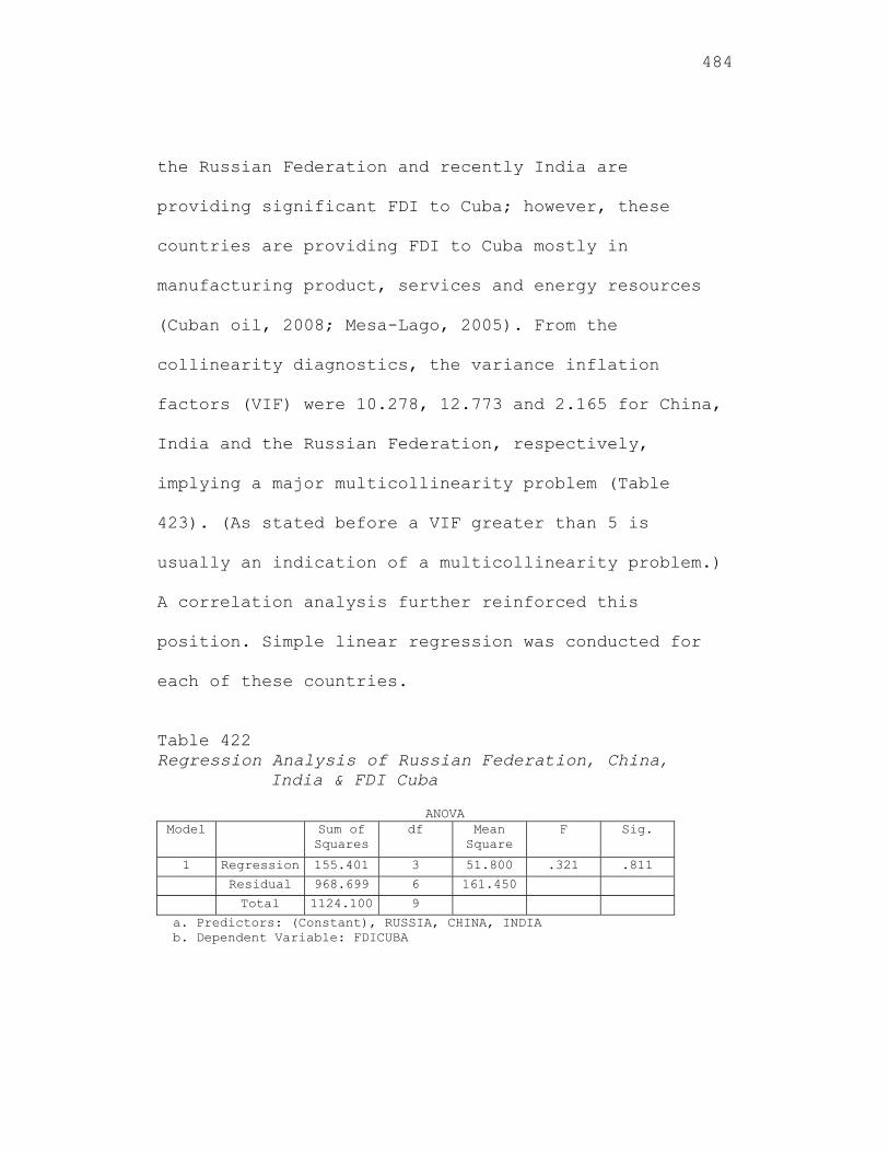
484

the Russian Federation and recently India are

providing significant FDI to Cuba; however, these

countries are providing FDI to Cuba mostly in

manufacturing product, services and energy resources

(Cuban oil, 2008; Mesa-Lago, 2005). From the

collinearity diagnostics, the variance inflation

factors (VIF) were 10.278, 12.773 and 2.165 for China,

India and the Russian Federation, respectively,

implying a major multicollinearity problem (Table

423). (As stated before a VIF greater than 5 is

usually an indication of a multicollinearity problem.)

A correlation analysis further reinforced this

position. Simple linear regression was conducted for

each of these countries.

Table 422 Regression Analysis of Russian Federation, China,

India & FDI Cuba

ANOVA Model Sum of

Squares df Mean

Square F Sig.

1 Regression 155.401 3 51.800 .321 .811

Residual 968.699 6 161.450

Total 1124.100 9

a. Predictors: (Constant), RUSSIA, CHINA, INDIA b. Dependent Variable: FDICUBA

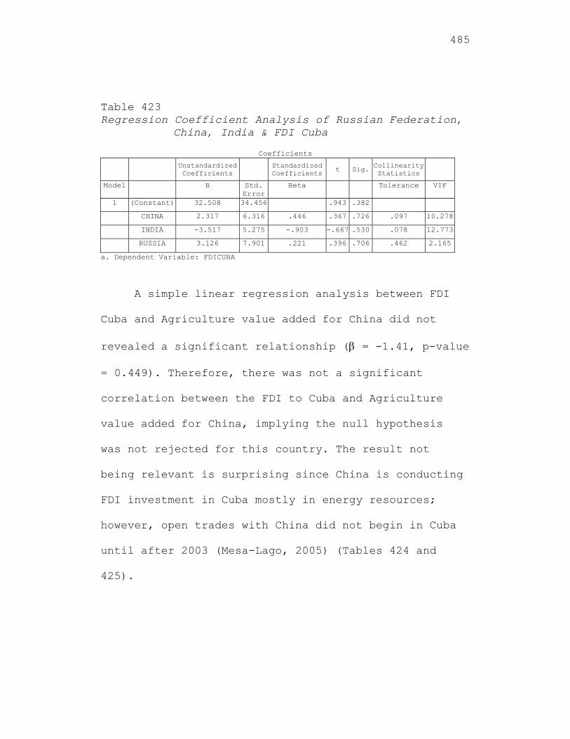
485

Table 423 Regression Coefficient Analysis of Russian Federation,

China, India & FDI Cuba

Coefficients Unstandardized

Coefficients Standardized

Coefficientst Sig. Collinearity

Statistics

Model B Std. Error

Beta Tolerance VIF

1 (Constant) 32.508 34.456 .943 .382

CHINA 2.317 6.316 .446 .367 .726 .097 10.278

INDIA -3.517 5.275 -.903 -.667 .530 .078 12.773

RUSSIA 3.126 7.901 .221 .396 .706 .462 2.165

a. Dependent Variable: FDICUBA

A simple linear regression analysis between FDI

Cuba and Agriculture value added for China did not

revealed a significant relationship ( = -1.41, p-value

= 0.449). Therefore, there was not a significant

correlation between the FDI to Cuba and Agriculture

value added for China, implying the null hypothesis

was not rejected for this country. The result not

being relevant is surprising since China is conducting

FDI investment in Cuba mostly in energy resources;

however, open trades with China did not begin in Cuba

until after 2003 (Mesa-Lago, 2005) (Tables 424 and

425).

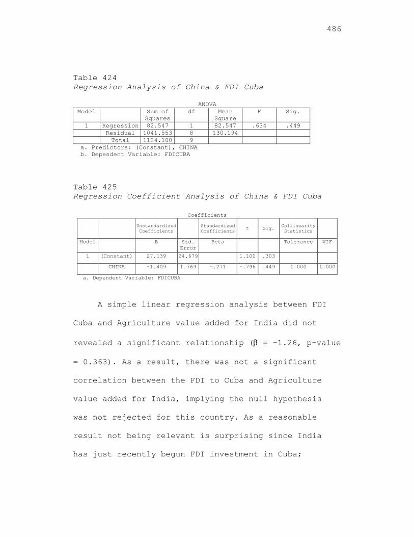
486

Table 424 Regression Analysis of China & FDI Cuba

ANOVA Model Sum of

Squares df Mean

Square F Sig.

1 Regression 82.547 1 82.547 .634 .449 Residual 1041.553 8 130.194 Total 1124.100 9

a. Predictors: (Constant), CHINA b. Dependent Variable: FDICUBA

Table 425 Regression Coefficient Analysis of China & FDI Cuba

Coefficients

Unstandardized Coefficients Standardized

Coefficients t Sig. Collinearity Statistics

Model B Std. Error

Beta Tolerance VIF

1 (Constant) 27.139 24.679 1.100 .303

CHINA -1.409 1.769 -.271 -.796 .449 1.000 1.000

a. Dependent Variable: FDICUBA

A simple linear regression analysis between FDI

Cuba and Agriculture value added for India did not

revealed a significant relationship ( = -1.26, p-value

= 0.363). As a result, there was not a significant

correlation between the FDI to Cuba and Agriculture

value added for India, implying the null hypothesis

was not rejected for this country. As a reasonable

result not being relevant is surprising since India

has just recently begun FDI investment in Cuba;

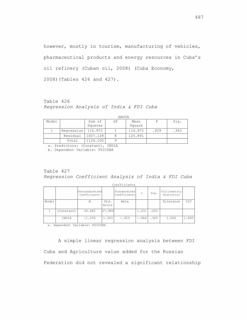
487

however, mostly in tourism, manufacturing of vehicles,

pharmaceutical products and energy resources in Cuba’s

oil refinery (Cuban oil, 2008) (Cuba Economy,

2008)(Tables 426 and 427).

Table 426 Regression Analysis of India & FDI Cuba

ANOVA Model Sum of

Squares df Mean

Square F Sig.

1 Regression 116.972 1 116.972 .929 .363 Residual 1007.128 8 125.891 Total 1124.100 9

a. Predictors: (Constant), INDIA b. Dependent Variable: FDICUBA

Table 427 Regression Coefficient Analysis of India & FDI Cuba

Coefficients

Unstandardized Coefficients Standardized

Coefficients t Sig. Collinearity Statistics

Model B Std. Error

Beta Tolerance VIF

1 (Constant) 34.462 27.989 1.231 .253

INDIA -1.256 1.303 -.323 -.964 .363 1.000 1.000

a. Dependent Variable: FDICUBA

A simple linear regression analysis between FDI

Cuba and Agriculture value added for the Russian

Federation did not revealed a significant relationship

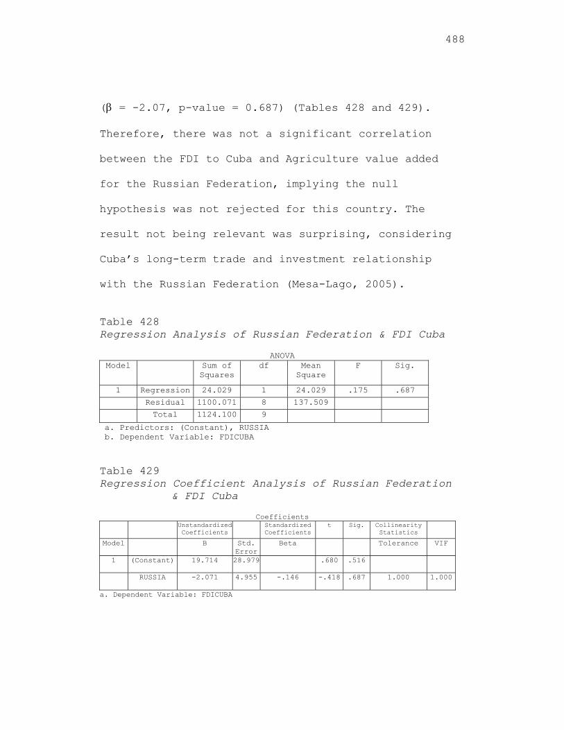
488

( = -2.07, p-value = 0.687) (Tables 428 and 429).

Therefore, there was not a significant correlation

between the FDI to Cuba and Agriculture value added

for the Russian Federation, implying the null

hypothesis was not rejected for this country. The

result not being relevant was surprising, considering

Cuba’s long-term trade and investment relationship

with the Russian Federation (Mesa-Lago, 2005).

Table 428 Regression Analysis of Russian Federation & FDI Cuba

ANOVA Model Sum of

Squares df Mean

Square F Sig.

1 Regression 24.029 1 24.029 .175 .687

Residual 1100.071 8 137.509

Total 1124.100 9

a. Predictors: (Constant), RUSSIA b. Dependent Variable: FDICUBA Table 429 Regression Coefficient Analysis of Russian Federation

& FDI Cuba

Coefficients Unstandardized

Coefficients Standardized

Coefficients t Sig. Collinearity

Statistics

Model B Std. Error

Beta Tolerance VIF

1 (Constant) 19.714 28.979 .680 .516

RUSSIA -2.071 4.955 -.146 -.418 .687 1.000 1.000

a. Dependent Variable: FDICUBA

489

Results for Category III (Least Developed Countries) Using the Independent Variable, Agriculture Value Added

The multiple regression analysis, with FDI to

Cuba as the dependent variable and Agriculture value

added for the least Developing countries, Jamaica,

Haiti, Peru, Madagascar and Nepal as the independent

variables did not revealed a significant relationship

(F value = 4.631 with a p-value = 0.081) (Table 430).

Therefore, there was not a significant correlation

between the FDI to Cuba and Agriculture value added

for the least developing countries of Jamaica, Haiti,

Peru, Madagascar and Nepal. Again, the beta

coefficients were not significant, implying the null

hypothesis was not rejected for these countries (Table

431). From the collinearity diagnostics, the variance

inflation factors for one of the five countries were

highly correlated with VIFs (variance inflation

factor) of 2.186, 3.341, 4.379, 2.521 and 7.346 for

Jamaica, Haiti, Peru, Madagascar and Nepal,

respectively. (VIF greater than 5 is usually an

indication of a multicollinearity problem.) A

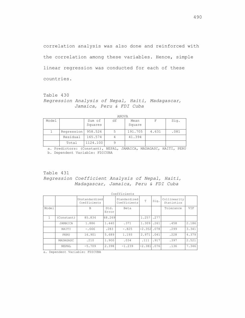
490

correlation analysis was also done and reinforced with

the correlation among these variables. Hence, simple

linear regression was conducted for each of these

countries.

Table 430 Regression Analysis of Nepal, Haiti, Madagascar,

Jamaica, Peru & FDI Cuba

ANOVA Model Sum of

Squares df Mean

Square F Sig.

1 Regression 958.526 5 191.705 4.631 .081

Residual 165.574 4 41.394

Total 1124.100 9

a. Predictors: (Constant), NEPAL, JAMAICA, MADAGASC, HAITI, PERU b. Dependent Variable: FDICUBA Table 431 Regression Coefficient Analysis of Nepal, Haiti,

Madagascar, Jamaica, Peru & FDI Cuba

Coefficients Unstandardized

Coefficients

Standardized Coefficients

T Sig.Collinearity Statistics

Model B Std. Error

Beta Tolerance VIF

1 (Constant) 85.834 68.269 1.257 .277

JAMAICA 1.886 1.440 .371 1.309 .261 .458 2.186

HAITI -.666 .283 -.825 -2.352 .078 .299 3.341

PERU 16.901 5.689 1.193 2.971 .041 .228 4.379

MADAGASC .210 1.900 .034 .111 .917 .397 2.521

NEPAL -5.709 2.398 -1.239 -2.381 .076 .136 7.346

a. Dependent Variable: FDICUBA

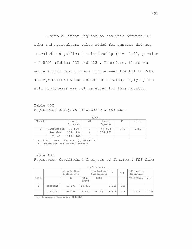
491

A simple linear regression analysis between FDI

Cuba and Agriculture value added for Jamaica did not

revealed a significant relationship ( = -1.07, p-value

= 0.559) (Tables 432 and 433). Therefore, there was

not a significant correlation between the FDI to Cuba

and Agriculture value added for Jamaica, implying the

null hypothesis was not rejected for this country.

Table 432 Regression Analysis of Jamaica & FDI Cuba

ANOVA Model Sum of

Squares df Mean

Square F Sig.

1 Regression 49.806 1 49.806 .371 .559 Residual 1074.294 8 134.287 Total 1124.100 9

a. Predictors: (Constant), JAMAICA b. Dependent Variable: FDICUBA Table 433 Regression Coefficient Analysis of Jamaica & FDI Cuba

Coefficients Unstandardized

Coefficients Standardized Coefficients t Sig.

Collinearity Statistics

Model B Std. Error

Beta Tolerance VIF

1 (Constant) 13.899 10.818 1.285 .235

JAMAICA -1.069 1.755 -.210 -.609 .559 1.000 1.000

a. Dependent Variable: FDICUBA

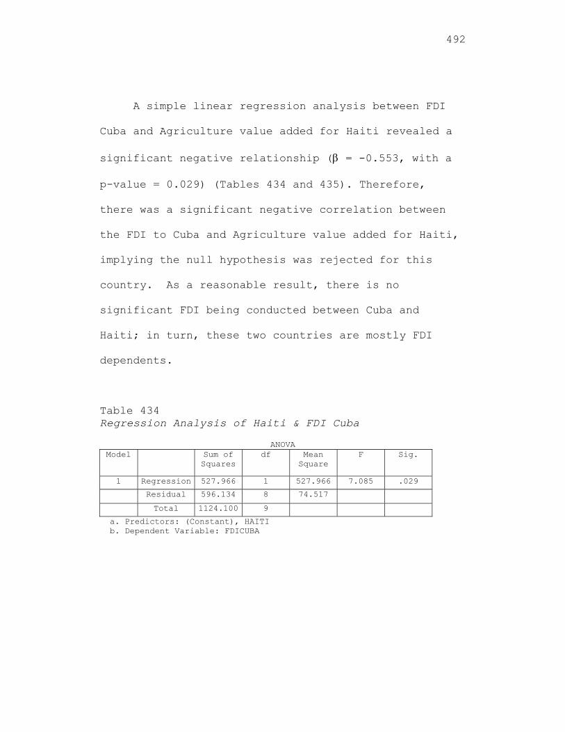
492

A simple linear regression analysis between FDI

Cuba and Agriculture value added for Haiti revealed a

significant negative relationship ( = -0.553, with a

p-value = 0.029) (Tables 434 and 435). Therefore,

there was a significant negative correlation between

the FDI to Cuba and Agriculture value added for Haiti,

implying the null hypothesis was rejected for this

country. As a reasonable result, there is no

significant FDI being conducted between Cuba and

Haiti; in turn, these two countries are mostly FDI

dependents.

Table 434 Regression Analysis of Haiti & FDI Cuba

ANOVA Model Sum of

Squares df Mean

Square F Sig.

1 Regression 527.966 1 527.966 7.085 .029

Residual 596.134 8 74.517

Total 1124.100 9

a. Predictors: (Constant), HAITI b. Dependent Variable: FDICUBA

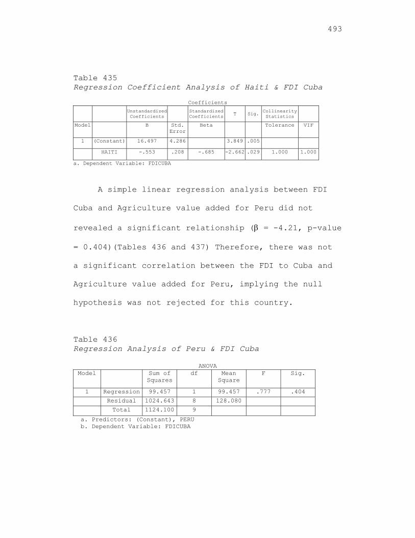
493

Table 435 Regression Coefficient Analysis of Haiti & FDI Cuba

Coefficients Unstandardized

Coefficients Standardized Coefficients T Sig.

Collinearity Statistics

Model B Std. Error

Beta Tolerance VIF

1 (Constant) 16.497 4.286 3.849 .005

HAITI -.553 .208 -.685 -2.662 .029 1.000 1.000

a. Dependent Variable: FDICUBA

A simple linear regression analysis between FDI

Cuba and Agriculture value added for Peru did not

revealed a significant relationship ( = -4.21, p-value

= 0.404)(Tables 436 and 437) Therefore, there was not

a significant correlation between the FDI to Cuba and

Agriculture value added for Peru, implying the null

hypothesis was not rejected for this country.

Table 436 Regression Analysis of Peru & FDI Cuba

ANOVA Model Sum of

Squares df Mean

Square F Sig.

1 Regression 99.457 1 99.457 .777 .404

Residual 1024.643 8 128.080

Total 1124.100 9

a. Predictors: (Constant), PERU b. Dependent Variable: FDICUBA

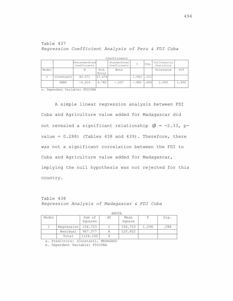
494

Table 437 Regression Coefficient Analysis of Peru & FDI Cuba

Coefficients Unstandardized

Coefficients Standardized Coefficients t Sig.

Collinearity Statistics

Model B Std. Error

Beta Tolerance VIF

1 (Constant) 40.571 37.474 1.083 .311

PERU -4.214 4.782 -.297 -.881 .404 1.000 1.000

a. Dependent Variable: FDICUBA

A simple linear regression analysis between FDI

Cuba and Agriculture value added for Madagascar did

not revealed a significant relationship ( = -2.33, p-

value = 0.288) (Tables 438 and 439). Therefore, there

was not a significant correlation between the FDI to

Cuba and Agriculture value added for Madagascar,

implying the null hypothesis was not rejected for this

country.

Table 438 Regression Analysis of Madagascar & FDI Cuba

ANOVA Model Sum of

Squares df Mean

Square F Sig.

1 Regression 156.723 1 156.723 1.296 .288 Residual 967.377 8 120.922 Total 1124.100 9

a. Predictors: (Constant), MADAGASC b. Dependent Variable: FDICUBA

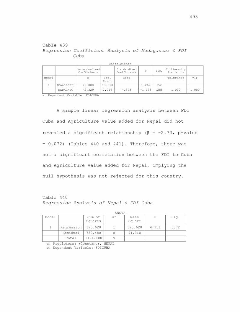
495

Table 439 Regression Coefficient Analysis of Madagascar & FDI

Cuba

Coefficients Unstandardized

Coefficients Standardized Coefficients T Sig. Collinearity

Statistics

Model B Std. Error

Beta Tolerance VIF

1 (Constant) 75.000 59.218 1.267 .241

MADAGASC -2.329 2.046 -.373 -1.138 .288 1.000 1.000

a. Dependent Variable: FDICUBA

A simple linear regression analysis between FDI

Cuba and Agriculture value added for Nepal did not

revealed a significant relationship ( = -2.73, p-value

= 0.072) (Tables 440 and 441). Therefore, there was

not a significant correlation between the FDI to Cuba

and Agriculture value added for Nepal, implying the

null hypothesis was not rejected for this country.

Table 440 Regression Analysis of Nepal & FDI Cuba

ANOVA Model Sum of

Squares df Mean

Square F Sig.

1 Regression 393.620 1 393.620 4.311 .072

Residual 730.480 8 91.310

Total 1124.100 9

a. Predictors: (Constant), NEPAL b. Dependent Variable: FDICUBA

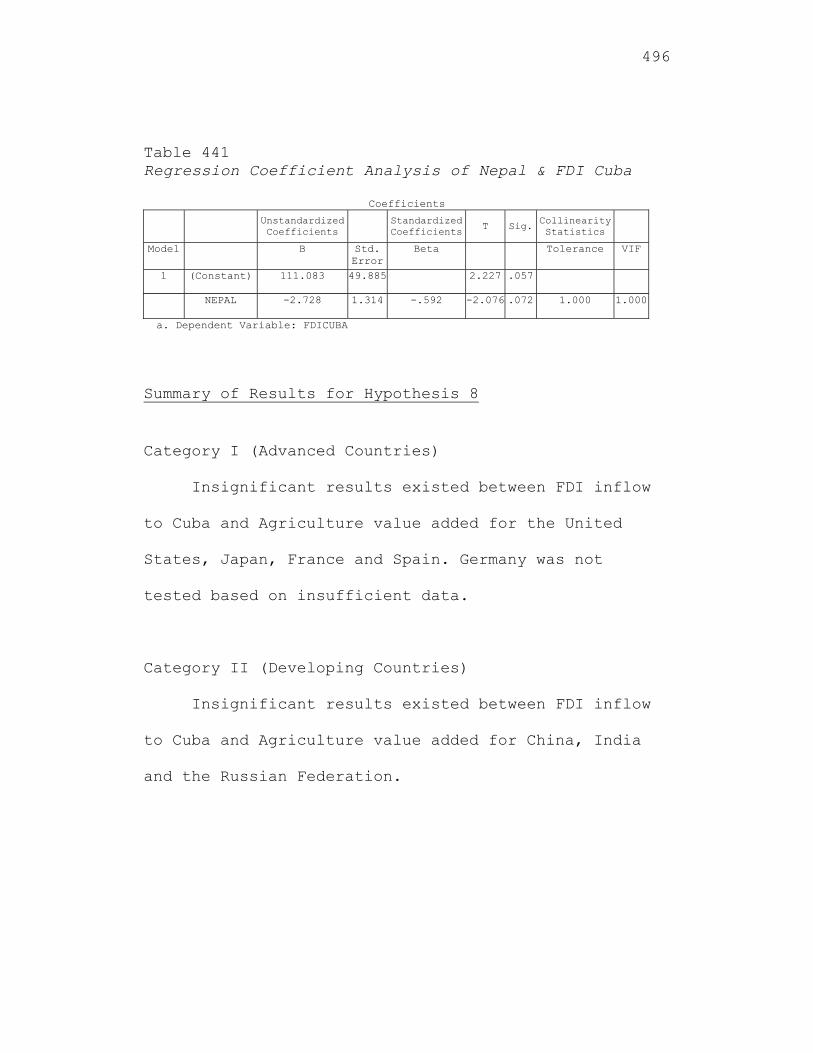
496

Table 441 Regression Coefficient Analysis of Nepal & FDI Cuba

Coefficients Unstandardized

Coefficients

Standardized Coefficients

T Sig.Collinearity Statistics

Model B Std. Error

Beta Tolerance VIF

1 (Constant) 111.083 49.885 2.227 .057

NEPAL -2.728 1.314 -.592 -2.076 .072 1.000 1.000

a. Dependent Variable: FDICUBA

Summary of Results for Hypothesis 8

Category I (Advanced Countries)

Insignificant results existed between FDI inflow

to Cuba and Agriculture value added for the United

States, Japan, France and Spain. Germany was not

tested based on insufficient data.

Category II (Developing Countries)

Insignificant results existed between FDI inflow

to Cuba and Agriculture value added for China, India

and the Russian Federation.

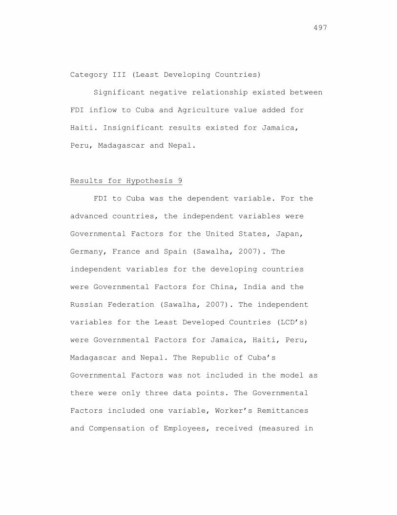
497

Category III (Least Developing Countries)

Significant negative relationship existed between

FDI inflow to Cuba and Agriculture value added for

Haiti. Insignificant results existed for Jamaica,

Peru, Madagascar and Nepal.

Results for Hypothesis 9

FDI to Cuba was the dependent variable. For the

advanced countries, the independent variables were

Governmental Factors for the United States, Japan,

Germany, France and Spain (Sawalha, 2007). The

independent variables for the developing countries

were Governmental Factors for China, India and the

Russian Federation (Sawalha, 2007). The independent

variables for the Least Developed Countries (LCD’s)

were Governmental Factors for Jamaica, Haiti, Peru,

Madagascar and Nepal. The Republic of Cuba’s

Governmental Factors was not included in the model as

there were only three data points. The Governmental

Factors included one variable, Worker’s Remittances

and Compensation of Employees, received (measured in

498

current US$). Worker’s remittances and Compensation of

Employees is part of a country’s labor system;

therefore, being part of the government.

The ninth hypothesis to be tested is:

Hypothesis H09: The level of contribution of

FDI inflow to Cuba is not significantly

related to the Governmental Factors for the

three groups of countries.

Hypothesis HA9: The level of contribution of

FDI inflow to Cuba is significantly related to

the Governmental Factors for the three groups

of countries.

The multiple regression models to test Hypothesis 9

are listed below.

Category I (Advanced Countries)

FDICUBA = αO + α1GOVERNMENTALFACTORSUS +

α2GOVERNMENTALFACTORSJapan +

499

α3GOVERNMENTALFACTORSGermany +

α4GOVERNMENTALFACTORSFrance +

α5GOVERNMENTALFACTORSSpain + ε1

Categories II (Developing Countries)

FDICUBA = O + 1GOVERNMENTALFACTORSChina +

2GOVERNMENTALFACTORSIndia +

3GOVERNMENTALFACTORSRussian Federation +ε2

Categories III (Least Developed Countries)

FDICUBA = δ + δ1GOVERNMENTALFACTORSJamaica +

δ2GOVERNMENTALFACTORSHaiti +

δ3GOVERNMENTALFACTORSPeru +

δ4GOVERNMENTALFACTORSMadagascar +

δ5GOVERNMENTALFACTORSNepal + ε3

The results were presented for the independent

variables measuring Worker’s Remittances and Employees

Compensation for each of the three categories of

countries.

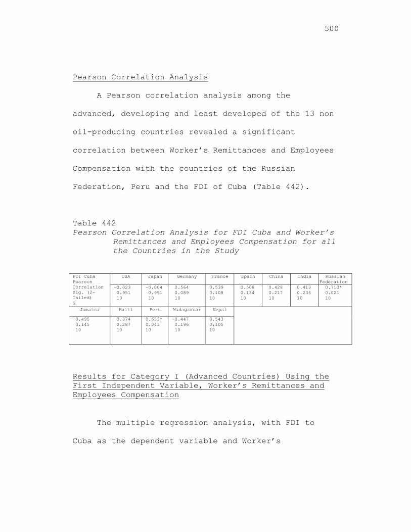
500

Pearson Correlation Analysis

A Pearson correlation analysis among the

advanced, developing and least developed of the 13 non

oil-producing countries revealed a significant

correlation between Worker’s Remittances and Employees

Compensation with the countries of the Russian

Federation, Peru and the FDI of Cuba (Table 442).

Table 442 Pearson Correlation Analysis for FDI Cuba and Worker’s

Remittances and Employees Compensation for all the Countries in the Study

FDI Cuba Pearson Correlation Sig. (2-Tailed) N

USA Japan Germany France Spain China India Russian Federation

-0.023 0.951 10

-0.004 0.991 10

0.564 0.089 10

0.539 0.108 10

0.508 0.134 10

0.428 0.217 10

0.413 0.235 10

0.710* 0.021 10

Jamaica Haiti Peru Madagascar Nepal

0.495 0.145 10

0.374 0.287 10

0.653* 0.041 10

-0.447 0.196 10

0.543 0.105 10

Results for Category I (Advanced Countries) Using the First Independent Variable, Worker’s Remittances and Employees Compensation

The multiple regression analysis, with FDI to

Cuba as the dependent variable and Worker’s

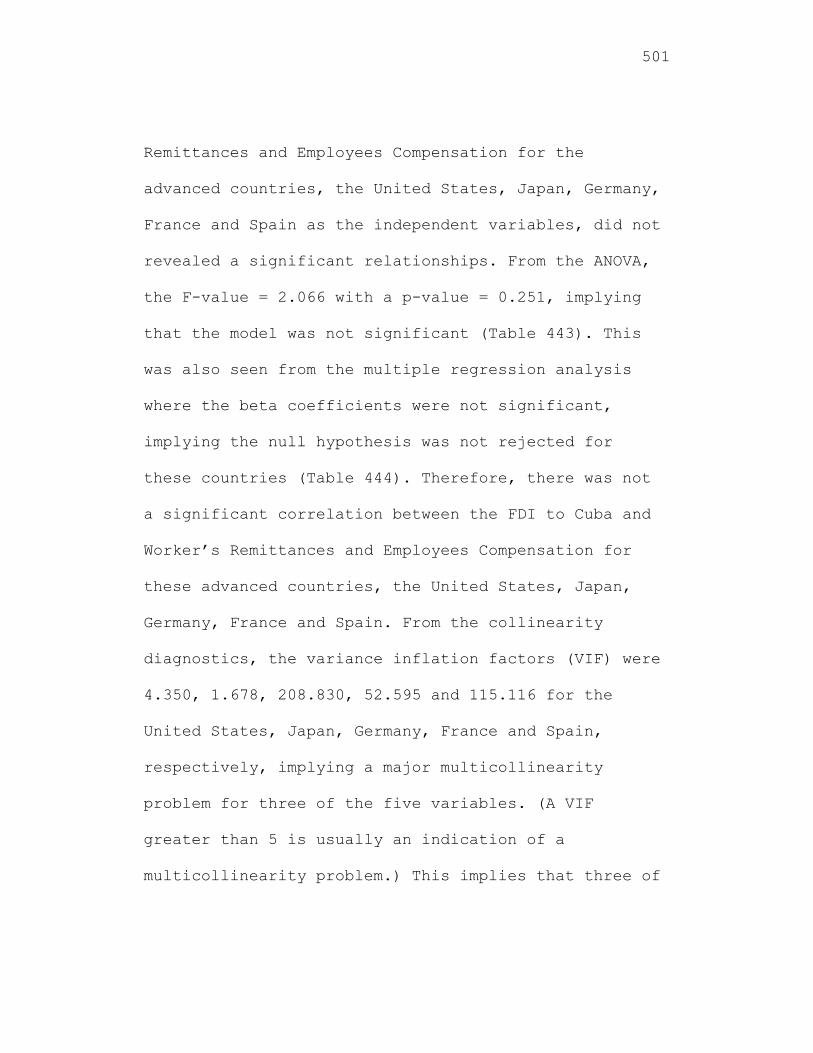
501

Remittances and Employees Compensation for the

advanced countries, the United States, Japan, Germany,

France and Spain as the independent variables, did not

revealed a significant relationships. From the ANOVA,

the F-value = 2.066 with a p-value = 0.251, implying

that the model was not significant (Table 443). This

was also seen from the multiple regression analysis

where the beta coefficients were not significant,

implying the null hypothesis was not rejected for

these countries (Table 444). Therefore, there was not

a significant correlation between the FDI to Cuba and

Worker’s Remittances and Employees Compensation for

these advanced countries, the United States, Japan,

Germany, France and Spain. From the collinearity

diagnostics, the variance inflation factors (VIF) were

4.350, 1.678, 208.830, 52.595 and 115.116 for the

United States, Japan, Germany, France and Spain,

respectively, implying a major multicollinearity

problem for three of the five variables. (A VIF

greater than 5 is usually an indication of a

multicollinearity problem.) This implies that three of

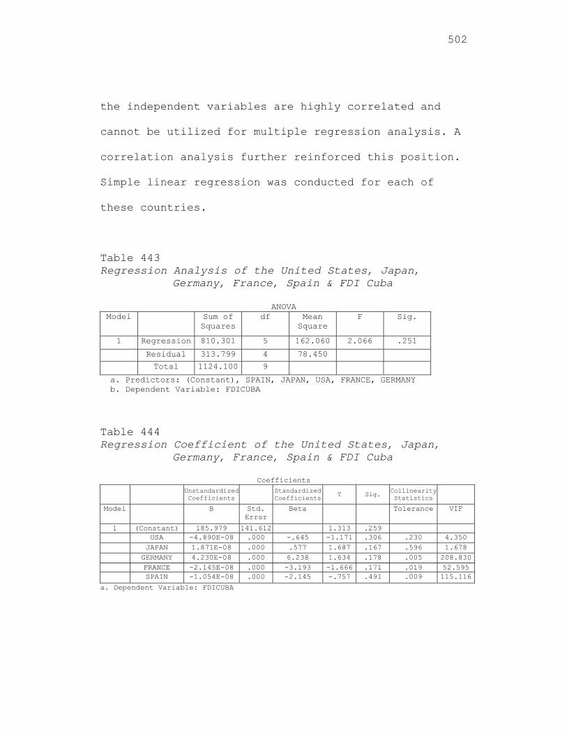
502

the independent variables are highly correlated and

cannot be utilized for multiple regression analysis. A

correlation analysis further reinforced this position.

Simple linear regression was conducted for each of

these countries.

Table 443 Regression Analysis of the United States, Japan,

Germany, France, Spain & FDI Cuba

ANOVA Model Sum of

Squares df Mean

Square F Sig.

1 Regression 810.301 5 162.060 2.066 .251

Residual 313.799 4 78.450

Total 1124.100 9

a. Predictors: (Constant), SPAIN, JAPAN, USA, FRANCE, GERMANY b. Dependent Variable: FDICUBA

Table 444 Regression Coefficient of the United States, Japan,

Germany, France, Spain & FDI Cuba

Coefficients Unstandardized

Coefficients Standardized Coefficients T Sig. Collinearity

Statistics

Model B Std. Error

Beta Tolerance VIF

1 (Constant) 185.979 141.612 1.313 .259 USA -4.890E-08 .000 -.645 -1.171 .306 .230 4.350 JAPAN 1.871E-08 .000 .577 1.687 .167 .596 1.678 GERMANY 4.230E-08 .000 6.238 1.634 .178 .005 208.830 FRANCE -2.145E-08 .000 -3.193 -1.666 .171 .019 52.595 SPAIN -1.054E-08 .000 -2.145 -.757 .491 .009 115.116

a. Dependent Variable: FDICUBA

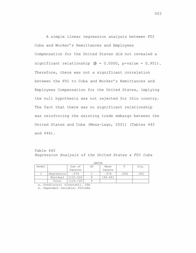
503

A simple linear regression analysis between FDI

Cuba and Worker’s Remittances and Employees

Compensation for the United States did not revealed a

significant relationship ( = 0.0000, p-value = 0.951).

Therefore, there was not a significant correlation

between the FDI to Cuba and Worker’s Remittances and

Employees Compensation for the United States, implying

the null hypothesis was not rejected for this country.

The fact that there was no significant relationship

was reinforcing the existing trade embargo between the

United States and Cuba (Mesa-Lago, 2001) (Tables 445

and 446).

Table 445 Regression Analysis of the United States & FDI Cuba

ANOVA Model Sum of

Squares df Mean

Square F Sig.

1 Regression .574 1 .574 .004 .951 Residual 1123.526 8 140.441 Total 1124.100 9

a. Predictors: (Constant), USA b. Dependent Variable: FDICUBA

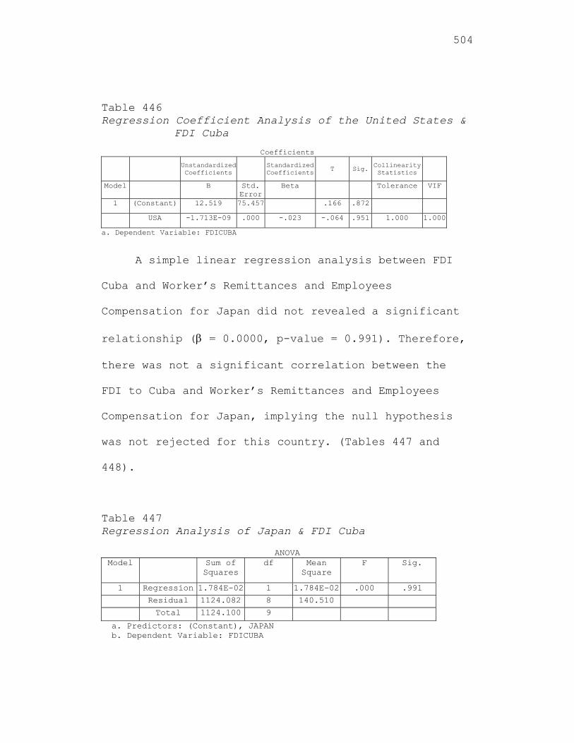
504

Table 446 Regression Coefficient Analysis of the United States &

FDI Cuba

Coefficients

Unstandardized Coefficients Standardized

Coefficients T Sig. Collinearity Statistics

Model B Std. Error

Beta Tolerance VIF

1 (Constant) 12.519 75.457 .166 .872

USA -1.713E-09 .000 -.023 -.064 .951 1.000 1.000

a. Dependent Variable: FDICUBA

A simple linear regression analysis between FDI

Cuba and Worker’s Remittances and Employees

Compensation for Japan did not revealed a significant

relationship ( = 0.0000, p-value = 0.991). Therefore,

there was not a significant correlation between the

FDI to Cuba and Worker’s Remittances and Employees

Compensation for Japan, implying the null hypothesis

was not rejected for this country. (Tables 447 and

448).

Table 447 Regression Analysis of Japan & FDI Cuba

ANOVA Model Sum of

Squares df Mean

Square F Sig.

1 Regression 1.784E-02 1 1.784E-02 .000 .991

Residual 1124.082 8 140.510

Total 1124.100 9

a. Predictors: (Constant), JAPAN b. Dependent Variable: FDICUBA

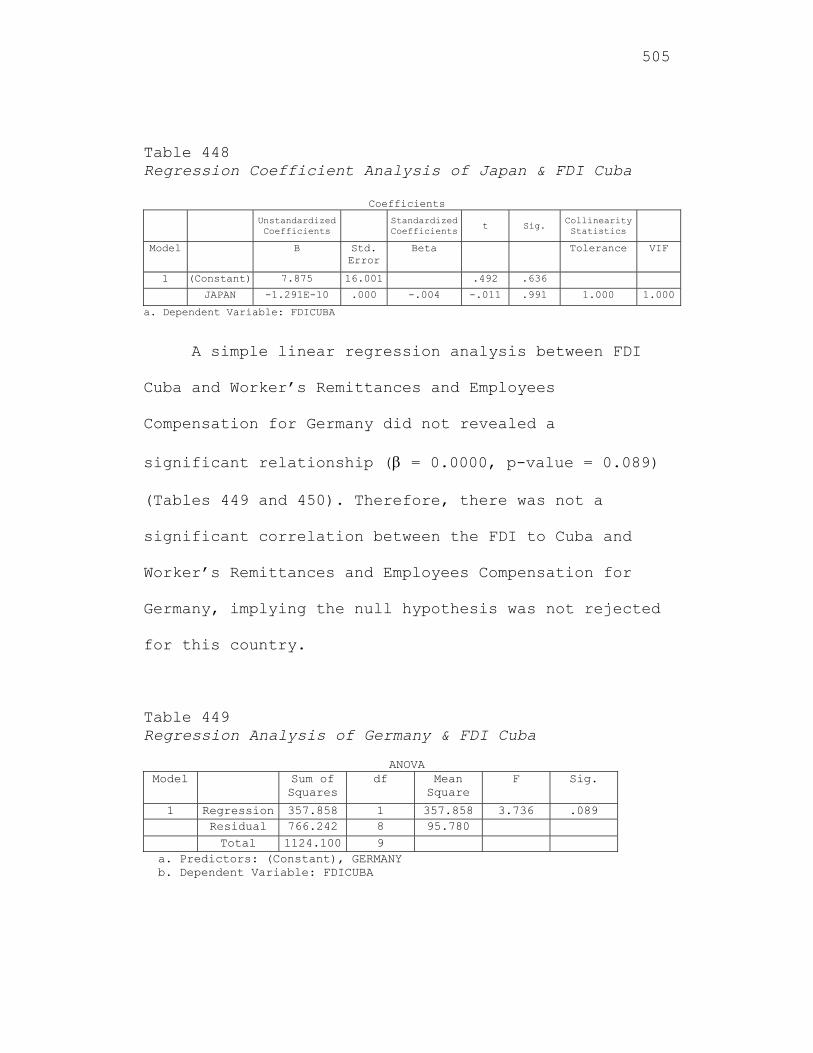
505

Table 448 Regression Coefficient Analysis of Japan & FDI Cuba

Coefficients Unstandardized

Coefficients Standardized Coefficients t Sig.

Collinearity Statistics

Model B Std. Error

Beta Tolerance VIF

1 (Constant) 7.875 16.001 .492 .636

JAPAN -1.291E-10 .000 -.004 -.011 .991 1.000 1.000

a. Dependent Variable: FDICUBA

A simple linear regression analysis between FDI

Cuba and Worker’s Remittances and Employees

Compensation for Germany did not revealed a

significant relationship ( = 0.0000, p-value = 0.089)

(Tables 449 and 450). Therefore, there was not a

significant correlation between the FDI to Cuba and

Worker’s Remittances and Employees Compensation for

Germany, implying the null hypothesis was not rejected

for this country.

Table 449 Regression Analysis of Germany & FDI Cuba

ANOVA Model Sum of

Squares df Mean

Square F Sig.

1 Regression 357.858 1 357.858 3.736 .089 Residual 766.242 8 95.780 Total 1124.100 9

a. Predictors: (Constant), GERMANY b. Dependent Variable: FDICUBA

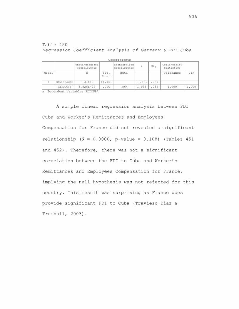
506

Table 450 Regression Coefficient Analysis of Germany & FDI Cuba

Coefficients Unstandardized

Coefficients Standardized Coefficients t Sig. Collinearity

Statistics

Model B Std. Error

Beta Tolerance VIF

1 (Constant) -13.610 11.451 -1.189 .269

GERMANY 3.826E-09 .000 .564 1.933 .089 1.000 1.000

a. Dependent Variable: FDICUBA

A simple linear regression analysis between FDI

Cuba and Worker’s Remittances and Employees

Compensation for France did not revealed a significant

relationship ( = 0.0000, p-value = 0.108) (Tables 451

and 452). Therefore, there was not a significant

correlation between the FDI to Cuba and Worker’s

Remittances and Employees Compensation for France,

implying the null hypothesis was not rejected for this

country. This result was surprising as France does

provide significant FDI to Cuba (Travieso-Diaz &

Trumbull, 2003).

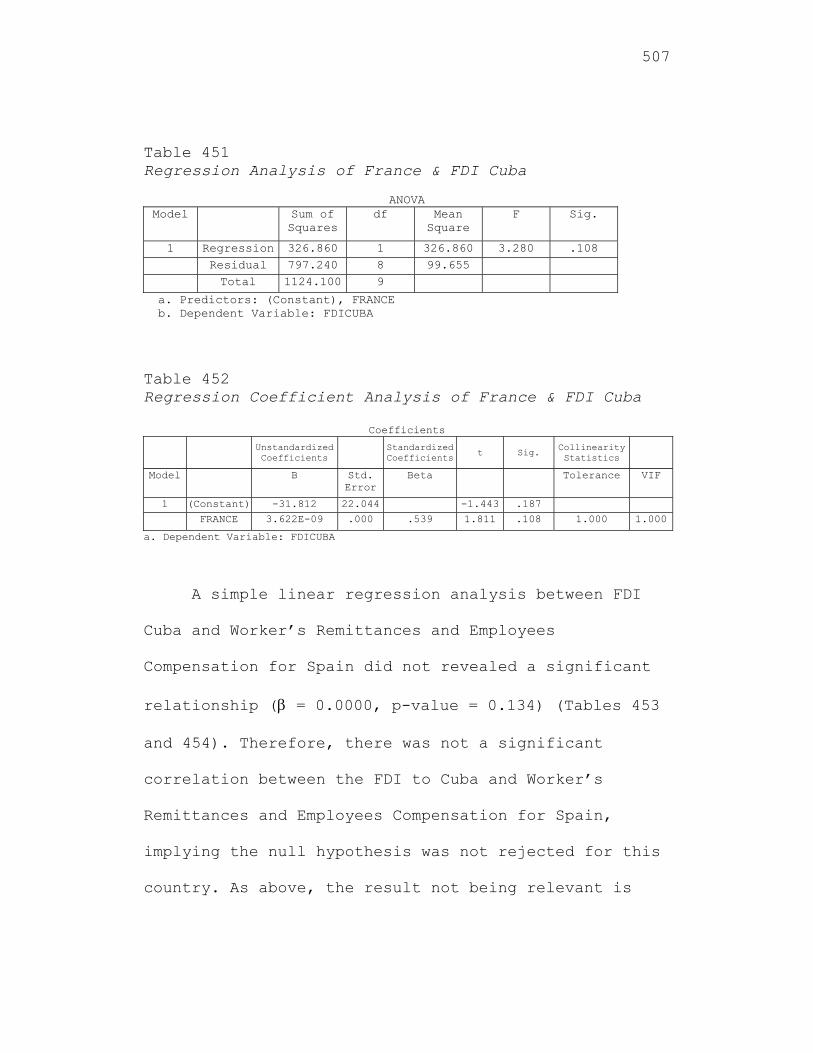
507

Table 451 Regression Analysis of France & FDI Cuba

ANOVA

Model Sum of Squares

df Mean Square

F Sig.

1 Regression 326.860 1 326.860 3.280 .108 Residual 797.240 8 99.655 Total 1124.100 9

a. Predictors: (Constant), FRANCE b. Dependent Variable: FDICUBA

Table 452 Regression Coefficient Analysis of France & FDI Cuba

Coefficients Unstandardized

Coefficients Standardized Coefficients t Sig. Collinearity

Statistics

Model B Std. Error

Beta Tolerance VIF

1 (Constant) -31.812 22.044 -1.443 .187

FRANCE 3.622E-09 .000 .539 1.811 .108 1.000 1.000

a. Dependent Variable: FDICUBA

A simple linear regression analysis between FDI

Cuba and Worker’s Remittances and Employees

Compensation for Spain did not revealed a significant

relationship ( = 0.0000, p-value = 0.134) (Tables 453

and 454). Therefore, there was not a significant

correlation between the FDI to Cuba and Worker’s

Remittances and Employees Compensation for Spain,

implying the null hypothesis was not rejected for this

country. As above, the result not being relevant is

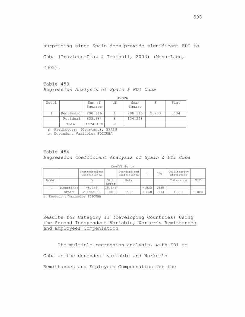
508

surprising since Spain does provide significant FDI to

Cuba (Travieso-Diaz & Trumbull, 2003) (Mesa-Lago,

2005).

Table 453 Regression Analysis of Spain & FDI Cuba

ANOVA

Model Sum of Squares

df Mean Square

F Sig.

1 Regression 290.116 1 290.116 2.783 .134

Residual 833.984 8 104.248

Total 1124.100 9

a. Predictors: (Constant), SPAIN b. Dependent Variable: FDICUBA Table 454 Regression Coefficient Analysis of Spain & FDI Cuba

Coefficients Unstandardized

Coefficients Standardized Coefficients t Sig. Collinearity

Statistics

Model B Std. Error

Beta Tolerance VIF

1 (Constant) -8.345 10.146 -.823 .435 SPAIN 2.496E-09 .000 .508 1.668 .134 1.000 1.000

a. Dependent Variable: FDICUBA

Results for Category II (Developing Countries) Using the Second Independent Variable, Worker’s Remittances and Employees Compensation

The multiple regression analysis, with FDI to

Cuba as the dependent variable and Worker’s

Remittances and Employees Compensation for the

509

developing countries, China, India and the Russian

Federation as the independent variables, did not

revealed a significant relationship. From the ANOVA,

the F-value = 3.834 with a p-value = 0.076, implying

that the model was not significant (Table 455).

Therefore, there was not a significant correlation

between the FDI to Cuba and Worker’s Remittances and

Employees Compensation for these developing countries

China, India and the Russian Federation, implying the

null hypothesis was not rejected for these countries.

From the collinearity diagnostics, the variance

inflation factors (VIF) were 25.797, 24.038 and 4.099

for China, India and the Russian Federation,

respectively, implying a major multicollinearity

problem for China and India (Table 456). (As stated

before a VIF greater than 5 is usually an indication

of a multicollinearity problem.) This implies that two

of the three independent variables are highly

correlated and cannot be utilized for multiple

regression analysis. A correlation analysis further

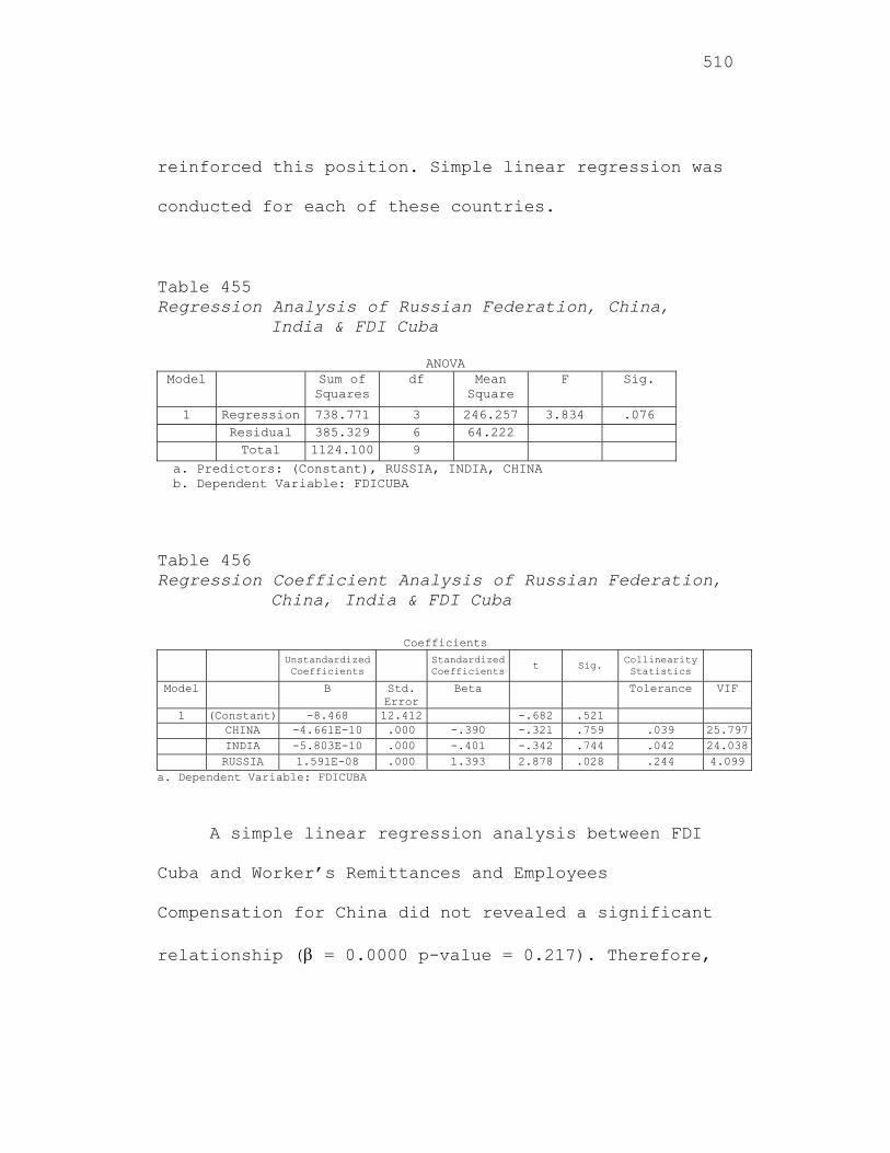
510

reinforced this position. Simple linear regression was

conducted for each of these countries.

Table 455 Regression Analysis of Russian Federation, China,

India & FDI Cuba

ANOVA Model Sum of

Squares df Mean

Square F Sig.

1 Regression 738.771 3 246.257 3.834 .076 Residual 385.329 6 64.222 Total 1124.100 9

a. Predictors: (Constant), RUSSIA, INDIA, CHINA b. Dependent Variable: FDICUBA

Table 456 Regression Coefficient Analysis of Russian Federation,

China, India & FDI Cuba

Coefficients Unstandardized

Coefficients Standardized Coefficients t Sig.

Collinearity Statistics

Model B Std. Error

Beta Tolerance VIF

1 (Constant) -8.468 12.412 -.682 .521 CHINA -4.661E-10 .000 -.390 -.321 .759 .039 25.797 INDIA -5.803E-10 .000 -.401 -.342 .744 .042 24.038 RUSSIA 1.591E-08 .000 1.393 2.878 .028 .244 4.099

a. Dependent Variable: FDICUBA

A simple linear regression analysis between FDI

Cuba and Worker’s Remittances and Employees

Compensation for China did not revealed a significant

relationship ( = 0.0000 p-value = 0.217). Therefore,

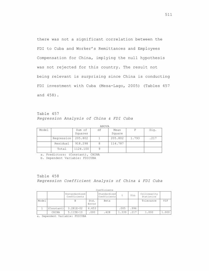
511

there was not a significant correlation between the

FDI to Cuba and Worker’s Remittances and Employees

Compensation for China, implying the null hypothesis

was not rejected for this country. The result not

being relevant is surprising since China is conducting

FDI investment with Cuba (Mesa-Lago, 2005) (Tables 457

and 458).

Table 457 Regression Analysis of China & FDI Cuba

ANOVA Model Sum of

Squares df Mean

Square F Sig.

Regression 205.802 1 205.802 1.793 .217

Residual 918.298 8 114.787

Total 1124.100 9

a. Predictors: (Constant), CHINA b. Dependent Variable: FDICUBA

Table 458 Regression Coefficient Analysis of China & FDI Cuba

Coefficients Unstandardized

Coefficients Standardized Coefficients t Sig. Collinearity

Statistics

Model B Std. Error

Beta Tolerance VIF

1 (Constant) 3.281E-02 6.653 .005 .996

CHINA 5.115E-10 .000 .428 1.339 .217 1.000 1.000

a. Dependent Variable: FDICUBA

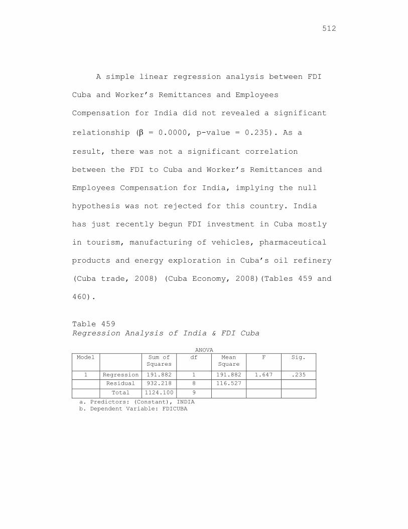
512

A simple linear regression analysis between FDI

Cuba and Worker’s Remittances and Employees

Compensation for India did not revealed a significant

relationship ( = 0.0000, p-value = 0.235). As a

result, there was not a significant correlation

between the FDI to Cuba and Worker’s Remittances and

Employees Compensation for India, implying the null

hypothesis was not rejected for this country. India

has just recently begun FDI investment in Cuba mostly

in tourism, manufacturing of vehicles, pharmaceutical

products and energy exploration in Cuba’s oil refinery

(Cuba trade, 2008) (Cuba Economy, 2008)(Tables 459 and

460).

Table 459 Regression Analysis of India & FDI Cuba

ANOVA Model Sum of

Squares df Mean

Square F Sig.

1 Regression 191.882 1 191.882 1.647 .235

Residual 932.218 8 116.527

Total 1124.100 9

a. Predictors: (Constant), INDIA b. Dependent Variable: FDICUBA

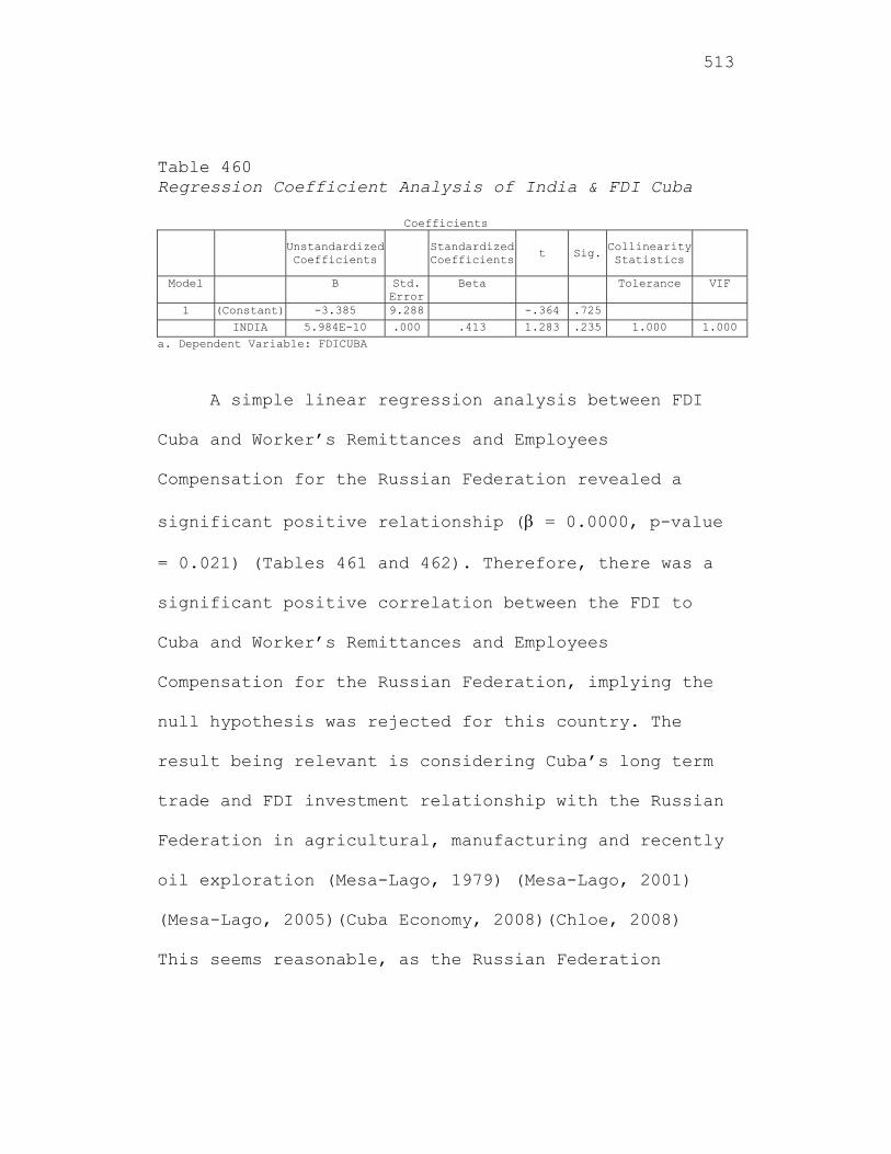
513

Table 460 Regression Coefficient Analysis of India & FDI Cuba

Coefficients

Unstandardized Coefficients

Standardized Coefficients t Sig.

Collinearity Statistics

Model B Std. Error

Beta Tolerance VIF

1 (Constant) -3.385 9.288 -.364 .725

INDIA 5.984E-10 .000 .413 1.283 .235 1.000 1.000

a. Dependent Variable: FDICUBA

A simple linear regression analysis between FDI

Cuba and Worker’s Remittances and Employees

Compensation for the Russian Federation revealed a

significant positive relationship ( = 0.0000, p-value

= 0.021) (Tables 461 and 462). Therefore, there was a

significant positive correlation between the FDI to

Cuba and Worker’s Remittances and Employees

Compensation for the Russian Federation, implying the

null hypothesis was rejected for this country. The

result being relevant is considering Cuba’s long term

trade and FDI investment relationship with the Russian

Federation in agricultural, manufacturing and recently

oil exploration (Mesa-Lago, 1979) (Mesa-Lago, 2001)

(Mesa-Lago, 2005)(Cuba Economy, 2008)(Chloe, 2008)

This seems reasonable, as the Russian Federation

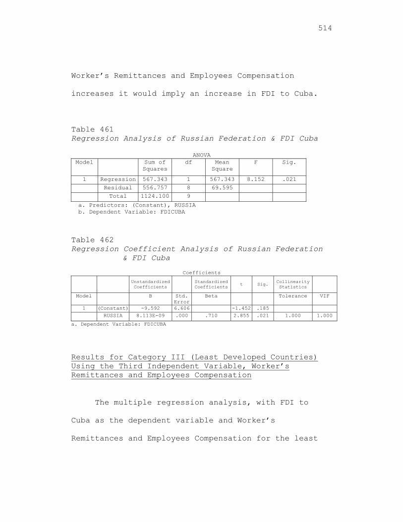
514

Worker’s Remittances and Employees Compensation

increases it would imply an increase in FDI to Cuba.

Table 461 Regression Analysis of Russian Federation & FDI Cuba

ANOVA Model Sum of

Squares df Mean

Square F Sig.

1 Regression 567.343 1 567.343 8.152 .021 Residual 556.757 8 69.595

Total 1124.100 9

a. Predictors: (Constant), RUSSIA b. Dependent Variable: FDICUBA

Table 462 Regression Coefficient Analysis of Russian Federation

& FDI Cuba

Coefficients

Unstandardized Coefficients Standardized

Coefficients t Sig. Collinearity Statistics

Model B Std. Error

Beta Tolerance VIF

1 (Constant) -9.592 6.606 -1.452 .185 RUSSIA 8.113E-09 .000 .710 2.855 .021 1.000 1.000

a. Dependent Variable: FDICUBA Results for Category III (Least Developed Countries) Using the Third Independent Variable, Worker’s Remittances and Employees Compensation

The multiple regression analysis, with FDI to

Cuba as the dependent variable and Worker’s

Remittances and Employees Compensation for the least

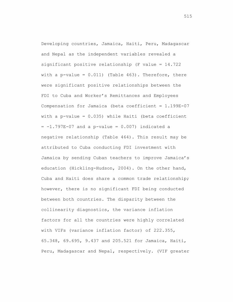
515

Developing countries, Jamaica, Haiti, Peru, Madagascar

and Nepal as the independent variables revealed a

significant positive relationship (F value = 14.722

with a p-value = 0.011) (Table 463). Therefore, there

were significant positive relationships between the

FDI to Cuba and Worker’s Remittances and Employees

Compensation for Jamaica (beta coefficient = 1.199E-07

with a p-value = 0.035) while Haiti (beta coefficient

= -1.797E-07 and a p-value = 0.007) indicated a

negative relationship (Table 464). This result may be

attributed to Cuba conducting FDI investment with

Jamaica by sending Cuban teachers to improve Jamaica’s

education (Hickling-Hudson, 2004). On the other hand,

Cuba and Haiti does share a common trade relationship;

however, there is no significant FDI being conducted

between both countries. The disparity between the

collinearity diagnostics, the variance inflation

factors for all the countries were highly correlated

with VIFs (variance inflation factor) of 222.355,

65.348, 69.695, 9.437 and 205.521 for Jamaica, Haiti,

Peru, Madagascar and Nepal, respectively. (VIF greater

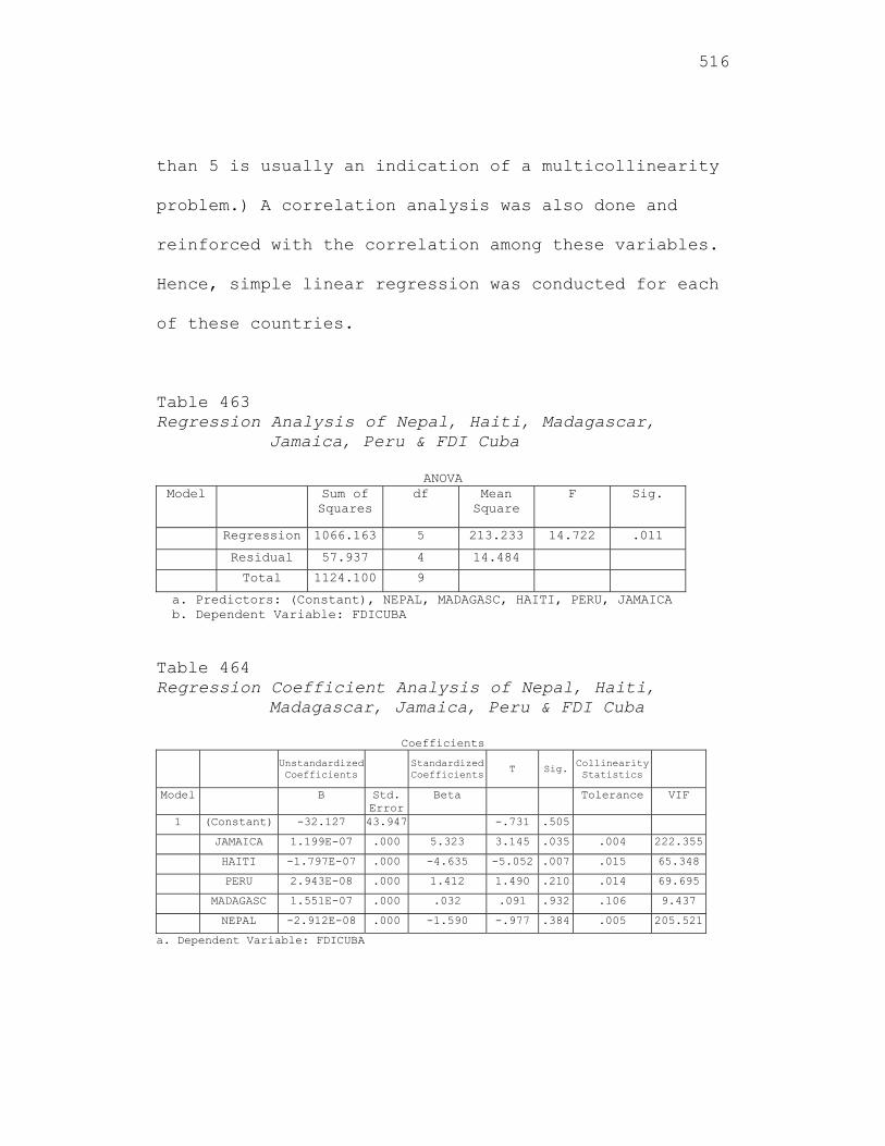
516

than 5 is usually an indication of a multicollinearity

problem.) A correlation analysis was also done and

reinforced with the correlation among these variables.

Hence, simple linear regression was conducted for each

of these countries.

Table 463 Regression Analysis of Nepal, Haiti, Madagascar,

Jamaica, Peru & FDI Cuba

ANOVA Model Sum of

Squares df Mean

Square F Sig.

Regression 1066.163 5 213.233 14.722 .011

Residual 57.937 4 14.484

Total 1124.100 9

a. Predictors: (Constant), NEPAL, MADAGASC, HAITI, PERU, JAMAICA b. Dependent Variable: FDICUBA Table 464 Regression Coefficient Analysis of Nepal, Haiti,

Madagascar, Jamaica, Peru & FDI Cuba

Coefficients

Unstandardized Coefficients Standardized

Coefficients T Sig. Collinearity Statistics

Model B Std. Error

Beta Tolerance VIF

1 (Constant) -32.127 43.947 -.731 .505

JAMAICA 1.199E-07 .000 5.323 3.145 .035 .004 222.355

HAITI -1.797E-07 .000 -4.635 -5.052 .007 .015 65.348

PERU 2.943E-08 .000 1.412 1.490 .210 .014 69.695

MADAGASC 1.551E-07 .000 .032 .091 .932 .106 9.437

NEPAL -2.912E-08 .000 -1.590 -.977 .384 .005 205.521

a. Dependent Variable: FDICUBA

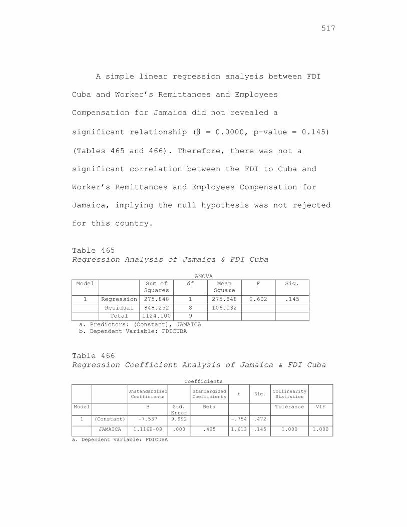
517

A simple linear regression analysis between FDI

Cuba and Worker’s Remittances and Employees

Compensation for Jamaica did not revealed a

significant relationship ( = 0.0000, p-value = 0.145)

(Tables 465 and 466). Therefore, there was not a

significant correlation between the FDI to Cuba and

Worker’s Remittances and Employees Compensation for

Jamaica, implying the null hypothesis was not rejected

for this country.

Table 465 Regression Analysis of Jamaica & FDI Cuba

ANOVA Model Sum of

Squares df Mean

Square F Sig.

1 Regression 275.848 1 275.848 2.602 .145

Residual 848.252 8 106.032 Total 1124.100 9

a. Predictors: (Constant), JAMAICA b. Dependent Variable: FDICUBA Table 466 Regression Coefficient Analysis of Jamaica & FDI Cuba

Coefficients

Unstandardized Coefficients Standardized

Coefficients t Sig. Collinearity Statistics

Model B Std. Error

Beta Tolerance VIF

1 (Constant) -7.537 9.992 -.754 .472

JAMAICA 1.116E-08 .000 .495 1.613 .145 1.000 1.000

a. Dependent Variable: FDICUBA

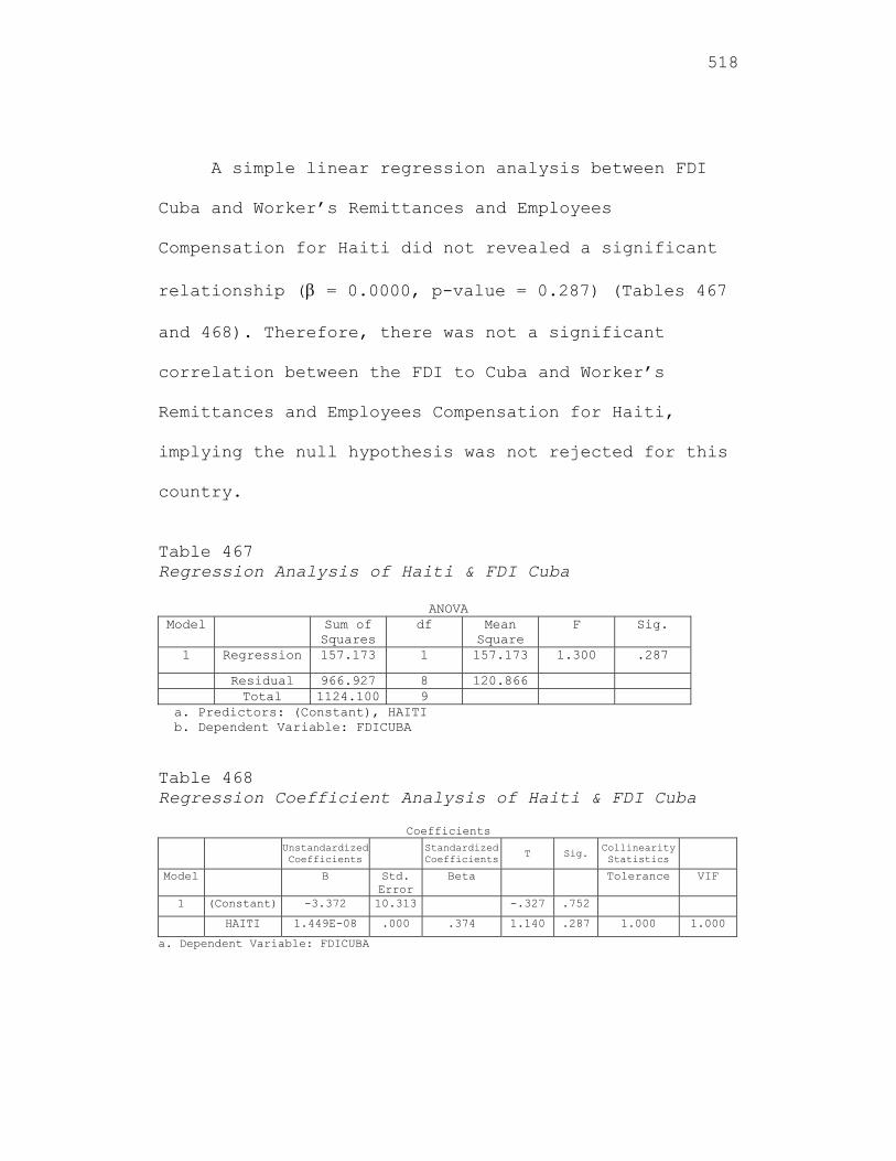
518

A simple linear regression analysis between FDI

Cuba and Worker’s Remittances and Employees

Compensation for Haiti did not revealed a significant

relationship ( = 0.0000, p-value = 0.287) (Tables 467

and 468). Therefore, there was not a significant

correlation between the FDI to Cuba and Worker’s

Remittances and Employees Compensation for Haiti,

implying the null hypothesis was not rejected for this

country.

Table 467 Regression Analysis of Haiti & FDI Cuba

ANOVA Model Sum of

Squares df Mean

Square F Sig.

1 Regression 157.173 1 157.173 1.300 .287

Residual 966.927 8 120.866 Total 1124.100 9

a. Predictors: (Constant), HAITI b. Dependent Variable: FDICUBA Table 468 Regression Coefficient Analysis of Haiti & FDI Cuba

Coefficients Unstandardized

Coefficients Standardized Coefficients T Sig. Collinearity

Statistics

Model B Std. Error

Beta Tolerance VIF

1 (Constant) -3.372 10.313 -.327 .752

HAITI 1.449E-08 .000 .374 1.140 .287 1.000 1.000

a. Dependent Variable: FDICUBA

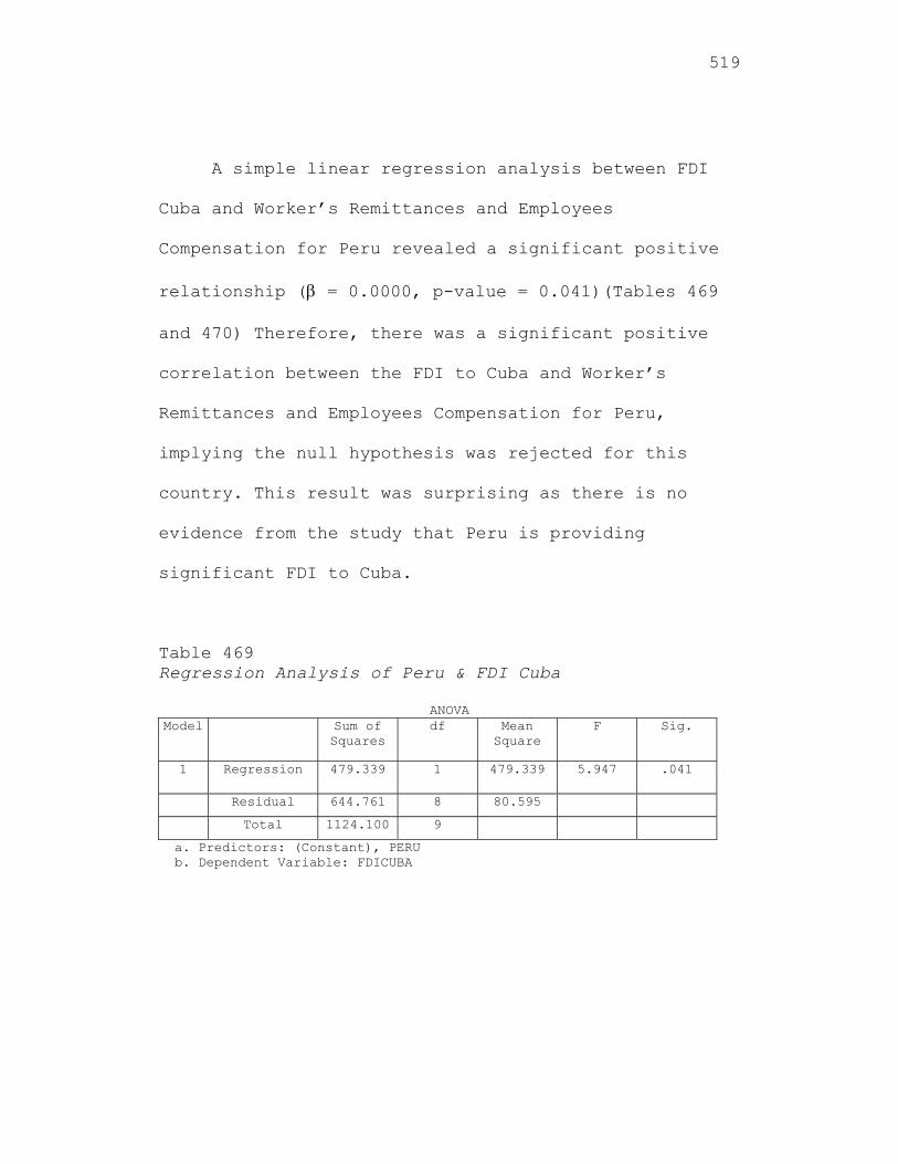
519

A simple linear regression analysis between FDI

Cuba and Worker’s Remittances and Employees

Compensation for Peru revealed a significant positive

relationship ( = 0.0000, p-value = 0.041)(Tables 469

and 470) Therefore, there was a significant positive

correlation between the FDI to Cuba and Worker’s

Remittances and Employees Compensation for Peru,

implying the null hypothesis was rejected for this

country. This result was surprising as there is no

evidence from the study that Peru is providing

significant FDI to Cuba.

Table 469 Regression Analysis of Peru & FDI Cuba

ANOVA Model Sum of

Squares df Mean

Square F Sig.

1 Regression 479.339 1 479.339 5.947 .041

Residual 644.761 8 80.595

Total 1124.100 9

a. Predictors: (Constant), PERU b. Dependent Variable: FDICUBA

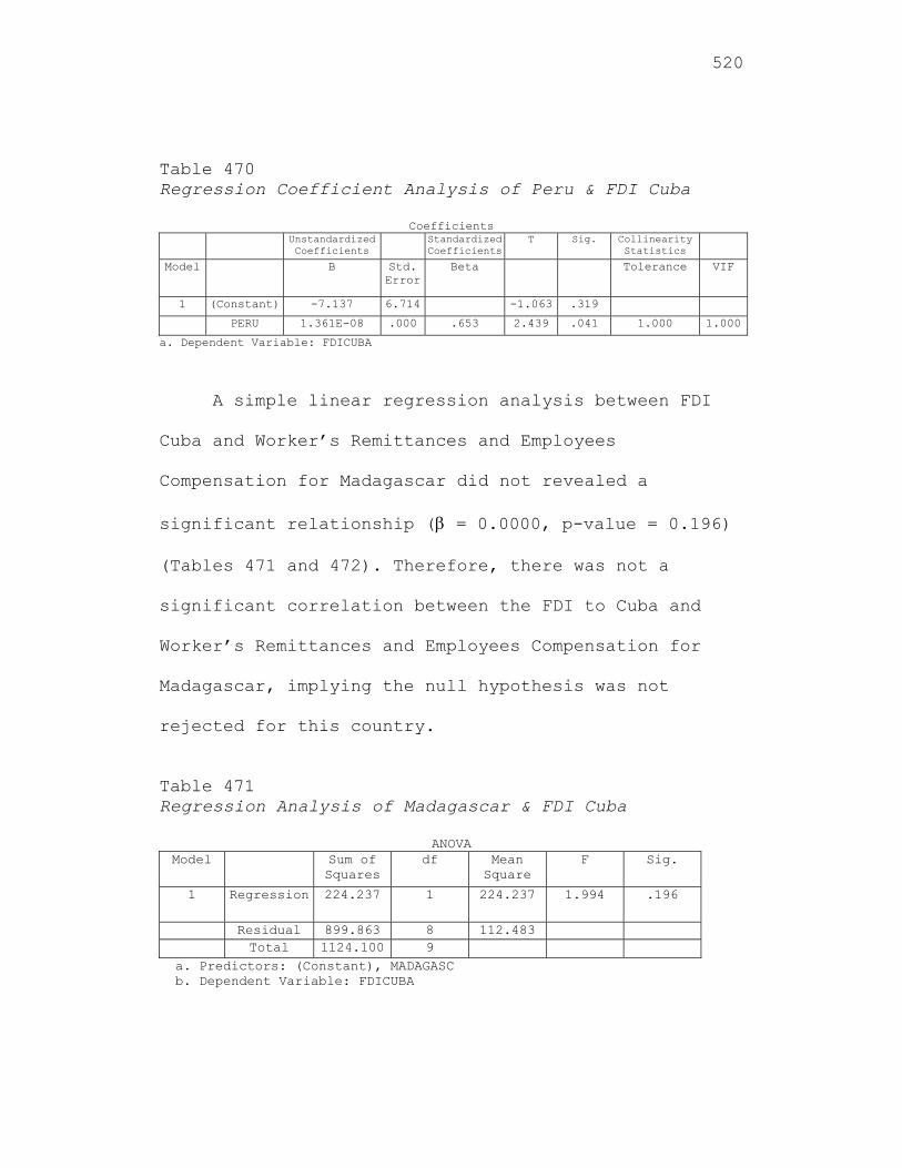
520

Table 470 Regression Coefficient Analysis of Peru & FDI Cuba

Coefficients Unstandardized

Coefficients Standardized

CoefficientsT Sig. Collinearity

Statistics

Model B Std. Error

Beta Tolerance VIF

1 (Constant) -7.137 6.714 -1.063 .319

PERU 1.361E-08 .000 .653 2.439 .041 1.000 1.000

a. Dependent Variable: FDICUBA

A simple linear regression analysis between FDI

Cuba and Worker’s Remittances and Employees

Compensation for Madagascar did not revealed a

significant relationship ( = 0.0000, p-value = 0.196)

(Tables 471 and 472). Therefore, there was not a

significant correlation between the FDI to Cuba and

Worker’s Remittances and Employees Compensation for

Madagascar, implying the null hypothesis was not

rejected for this country.

Table 471 Regression Analysis of Madagascar & FDI Cuba

ANOVA Model Sum of

Squares df Mean

Square F Sig.

1 Regression 224.237 1 224.237 1.994 .196

Residual 899.863 8 112.483 Total 1124.100 9

a. Predictors: (Constant), MADAGASC b. Dependent Variable: FDICUBA

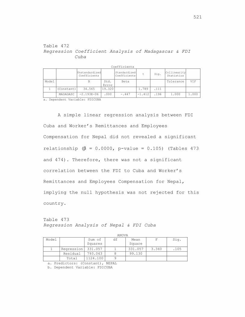
521

Table 472 Regression Coefficient Analysis of Madagascar & FDI

Cuba

Coefficients

Unstandardized Coefficients Standardized

Coefficients t Sig. Collinearity Statistics

Model B Std. Error

Beta Tolerance VIF

1 (Constant) 34.565 19.320 1.789 .111

MADAGASC -2.193E-06 .000 -.447 -1.412 .196 1.000 1.000

a. Dependent Variable: FDICUBA

A simple linear regression analysis between FDI

Cuba and Worker’s Remittances and Employees

Compensation for Nepal did not revealed a significant

relationship ( = 0.0000, p-value = 0.105) (Tables 473

and 474). Therefore, there was not a significant

correlation between the FDI to Cuba and Worker’s

Remittances and Employees Compensation for Nepal,

implying the null hypothesis was not rejected for this

country.

Table 473 Regression Analysis of Nepal & FDI Cuba

ANOVA Model Sum of

Squares df Mean

Square F Sig.

1 Regression 331.057 1 331.057 3.340 .105 Residual 793.043 8 99.130 Total 1124.100 9

a. Predictors: (Constant), NEPAL b. Dependent Variable: FDICUBA

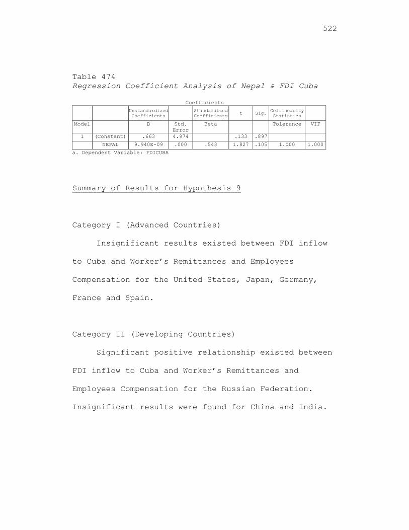
522

Table 474 Regression Coefficient Analysis of Nepal & FDI Cuba

Coefficients Unstandardized

Coefficients Standardized Coefficients t Sig. Collinearity

Statistics

Model B Std. Error

Beta Tolerance VIF

1 (Constant) .663 4.974 .133 .897

NEPAL 9.940E-09 .000 .543 1.827 .105 1.000 1.000

a. Dependent Variable: FDICUBA

Summary of Results for Hypothesis 9

Category I (Advanced Countries)

Insignificant results existed between FDI inflow

to Cuba and Worker’s Remittances and Employees

Compensation for the United States, Japan, Germany,

France and Spain.

Category II (Developing Countries)

Significant positive relationship existed between

FDI inflow to Cuba and Worker’s Remittances and

Employees Compensation for the Russian Federation.

Insignificant results were found for China and India.

523

Category III (Least Developing Countries)

Multiple regression results are not appropriate

when there are multicollinearity problems. Significant

positive relationship existed between FDI inflow to

Cuba and Worker’s Remittances and Employees

Compensation for Peru, while insignificant results

were found for Jamaica, Haiti, Madagascar and Nepal.

524

CHAPTER 5

CONCLUSION

Introduction

This chapter summarized the empirical results

from Chapter 4. All nine hypotheses were discussed and

a summary of the results was presented for the 13

countries in the study. The theoretical and practical

implications were also discussed, as well as, the

limitation of this study and suggestions for future

research.

Overview

The research was about the relationship between

FDI inflows to Cuba and macroeconomic variables from

13 countries. These countries were grouped into three

different categories, advanced countries, developing

countries and least developed countries. The countries

classified as advanced countries were United States,

Japan, France, Germany and Spain. The developing

525

countries were China, India and the Russian Federation

and the least developed countries were Jamaica, Haiti,

Peru, Madagascar and Nepal. The variables tested were

GNI per capita, Financial Capital, Level of

Technology, Human Capital, Energy and Natural

Resources, Transportation and Communication, Market

Type, Environment Factors and Governmental Factors.

Summary of the Findings

The findings for the thirteen countries,

categorized as advanced, developing, and less

developed, were as follows.

The results for Hypothesis 1, FDI to Cuba was

significantly related to GNI per capita, were shown

for the three categories of countries (Table 468). For

Category I countries, significant positive

relationships were found for Germany, France and

Spain. This was a reasonable result since these

European countries invested in Cuba. Insignificant

results were found for the United States and Japan.

The findings for the United States were not surprising

526

and supported the effectiveness of U.S. trade embargo

with Cuba. The findings for Japan were also not

surprising because Japan did not have a very strong

political and economic relationship with Cuba. For

category II countries, significant positive

relationship existed between FDI inflow to Cuba and

GNI per capita for the Russian Federation. This was a

reasonable result since the Russian Federation has a

long political and economic relationship with Cuba

(Mesa-Lago, 2005). Insignificant results were found

for China while India showed a marginal positive

result. China’s relationship with Cuba was primarily

based on similar political agendas and hence, GNI per

capita did not appear significant. India’s marginal

significant result reinforced India’s investments in

Cuba. For Category III countries, significant positive

relationship existed between FDI inflow to Cuba and

GNI per capita for Peru. This was a surprising result,

since Peru was not providing significant FDI to Cuba.

Insignificant results were found for Jamaica, Haiti,

Madagascar and Nepal indicating no correlation among

527

the GNI per capita of these countries and FDI to Cuba.

The results for these developing countries were

reasonable as these countries contributed minimally to

FDI.

The results for Hypothesis 2, FDI to Cuba was

significantly related to financial capital formation

in the thirteen countries, were shown below. Two

independent variables, gross fixed capital formation

and gross capital formation, were used to test this

hypothesis. Empirical findings for the first

independent variable, gross fixed capital formation,

revealed insignificant relationships for all

Categories I countries (United States, Japan, France,

Germany and Spain). For the second independent

variable, gross capital formation, similar

insignificants results were found for these Category I

countries. Hence, capital formation in these developed

countries was not significantly related to FDI to

Cuba. The insignificance of capital formation in the

U.S. and Japan with FDI to Cuba was not surprising.

However, the insignificant results for France, Germany

528

and Spain were surprising. Perhaps, the FDI to Cuba

from these countries was small compared to the value

of capital formation per year. Using gross fixed

capital formation for Category II countries, a

significant positive relationship was found for India.

This was a reasonable result as India was providing

FDI to Cuba (Cuba trade, 2008). Insignificant

relationships were found for China and the Russian

Federation. As stated before, insignificant results

for China were reasonable. However, insignificant

results for the Russian Federation were surprising,

considering the strong political and economic ties

that it had with Cuba. For the next independent

variable, gross capital formation for Category II

countries, insignificant relationship existed for

China and the Russian Federation. However, a marginal

positive relationship was found for India, a

reasonable result as India had been providing

significant FDI to Cuba (Cuba trade, 2008). Using

gross fixed capital formation for Category III

countries, insignificant relationship existed for

529

Jamaica, Haiti, Peru, Madagascar and Nepal. For gross

capital formation for Category III countries,

insignificant relationship existed for Jamaica, Haiti,

Peru and Madagascar. Again, these insignificant

results for these less developing countries were

reasonable. A marginal positive relationship between

FDI to Cuba and gross capital formation was found for

Nepal. There was no clear justification for this

result and hence it was most likely a spurious

correlation.

The results for Hypothesis 3, FDI to Cuba was

significantly related to the level of technology in

the thirteen countries, were shown below. Two

independent variables, high technology and industry

value added, were used to test this hypothesis.

Empirical findings for high technology exports

revealed insignificant relationships for three

Category I countries, United States, Germany and

France. Japan and Spain revealed a marginally

significant negative relationship. Using the next

independent variable, industry value added for

530

Category I countries, significant positive

relationship existed for Spain. Spain was Cuba’s

largest trading partner in Europe (McPherson &

Trumbull, 2007). Insignificant results were found for

the United States, Japan, France and Germany. Using

high technology exports for Category II countries,

significant positive relationship existed for China,

India and the Russian Federation. As these countries

increased their high technology exports, they

increased their foreign earnings. This would lead to

more FDI to other countries, including Cuba. For the

next independent variable, industry value added,

significant positive relationship existed for China.

As China’s industries added more value they were able

to generate more foreign earnings and hence had more

FDI to assist other countries, including Cuba. For

this hypothesis, level of technology in China was

significantly related to FDI to Cuba. Insignificant

results were found for the Russian Federation. This

was a surprising result as the Russian Federation was

assisting Cuba in many areas. A marginal positive

531

relationship was found for India. This marginal

significant relationship for India was supporting

India’s increasing FDI to Cuba. Using high technology

exports for Category III, insignificant relationship

existed for Jamaica, Peru and Madagascar. This was not

a surprising result. Nepal and Haiti were not tested

due to insufficient data. For the next independent

variable, industry value added, significant positive

relationship existed for Peru. This was a surprising

result, since Cuba was not receiving FDI from Peru.

Insignificant results were found for Jamaica, Haiti,

Madagascar and Nepal. Again, this was not a surprising

result for these less developed countries.

The results for Hypothesis 4, FDI to Cuba was

significantly related to the human capital in the

thirteen countries, were shown below. Two independent

variables, school enrollment and total unemployment

were used to test this hypothesis. Empirical findings

for school enrollment revealed insignificant

relationships for Category I countries (United States,

Japan, France, Germany and Spain). Hence, in these

532

advanced countries, school enrollment, a proxy for

human development, did not affect FDI in Cuba. For

total unemployment, similar insignificants results

were found for these Category I countries, except for

Japan, which revealed a significant negative

relationship. As unemployment increased in Japan, FDI

to Cuba went down – a reasonable result.

Using school enrollment for Category II

countries, revealed insignificant relationship for

China, India and the Russian Federation. Hence, school

enrollment, a proxy for human development in these

developing countries did not affect FDI in Cuba. For

the next independent variable, total unemployment,

similar insignificants results were found for these

Category II countries. Using school enrollment for

Category III countries revealed a significant positive

relationship for Nepal. This was not a reasonable

result, since Nepal was not providing FDI to Cuba.

This was most likely spurious correlation. Jamaica and

Haiti revealed significant negative relationships

between school enrollment and FDI to Cuba. Hence, when

533

the school enrollment in these two countries went up,

FDI to Cuba went down. This meant that as these

countries put more resources in education less was

available for FDI. Results for Jamaica were reasonable

as Jamaica had been investing in Cuba. The results for

Haiti were surprising. Insignificant results were

found for Peru, while a marginal positive relationship

was found for Madagascar. Insignificant findings for

Peru were not surprising. However, significant results

for Madagascar were surprising as this country did not

have any economic and political connection with Cuba.

For total unemployment, insignificants results were

found for these Category III countries – reasonable

results.

The results for Hypothesis 5, FDI to Cuba were

significantly related to the energy and natural

resources in the thirteen countries, were shown below.

Two independent variables, energy use and fuel

imports, were used to test this hypothesis. Empirical

findings for energy use revealed insignificant

relationships for Category I countries (United States,

534

Japan, Germany, France and Spain). For the next

independent variable, fuel imports, similar

insignificants results were found for these Category I

countries. Hence, energy use in these advanced

countries did not impact FDI to Cuba. Using energy use

for Category II countries revealed insignificant

relationship for China, India and the Russian

Federation. For fuel imports, similar insignificants

results were found for these Category II countries.

Hence, like the advanced countries, energy use in

these developing countries had no impact on FDI to

Cuba. Using energy use for Category III countries

revealed a significant positive relationship for

Haiti. This was a surprising result. Insignificant

results were found for Jamaica, Peru and Nepal, while

Madagascar was not tested due to insufficient data.

Insignificant results for these less developed

countries were reasonable. For fuel imports, similar

insignificants results were found for Jamaica and

Nepal – reasonable results. However, Peru showed a

positive marginal result – a surprising result. Also,

535

Madagascar revealed a significant negative

relationship. This again was a surprising result.

Haiti was not tested due to insufficient data.

The results for Hypothesis 6, FDI to Cuba was

significantly related to the transportation and

communication in the thirteen countries, were shown

below. Three independent variables, air transport,

fixed line/mobile phone subscribers and internet

users, were used to test this hypothesis. Empirical

findings for the three independent variables, air

transport, fixed line/mobile phone subscribers and

internet users, revealed insignificant relationships

for Category I countries (United States, Japan,

Germany, France and Spain). Hence, communication and

transportation in these advanced countries were not

related to FDI to Cuba. Using air transport, and fixed

line and mobile phone subscribers for Category II

countries revealed insignificant relationships for

China, India and the Russian Federation. For the

variable, internet users, similar insignificants

results were found for China and the Russian

536

Federation. However, India showed a significant

positive relationship between internet users and FDI

to Cuba. As India’s internet use increased so did

Cuba’s FDI. As stated before, India had been investing

in Cuba’s economy (Cuba economy, 2008) and (Cuba

trade, 2008). Using air transport for Category III

countries revealed insignificant relationship for

Peru, Madagascar and Nepal. A marginal negative

relationship was found for Jamaica, while Haiti was

not tested due to insufficient data. For the

independent variable, fixed line and mobile phone

subscribers, similar insignificants results were found

for these Category III countries. In addition, for the

variable, internet users, insignificant relationships

were found for Jamaica, Haiti, Peru and Nepal. These

were reasonable results for less developed countries.

Madagascar was not tested due to insufficient data.

The results for Hypothesis 7, FDI to Cuba was

significantly related to the market type in the

thirteen countries, were shown below. The independent

variable, merchandise trade, was used to test this

537

hypothesis. Insignificant relationships existed for

Category I countries, United States, Germany, France

and Spain. A marginal positive relationship was found

for Japan, corroborating its FDI investment with Cuba

(McPherson & Trumbull, 2007). Using merchandise trade

for Category II countries revealed insignificant

relationship for China and the Russian Federation,

while India showed a marginal positive result. Using

merchandise trade for Category III countries revealed

a significant positive relationship for Jamaica, a

reasonable result considering Jamaica’s investment in

Cuba, particularly in the travel/tourism industry

(Journal of Commerce, 1998) (Mesa-Lago, 2005).

Insignificant relationships were found for Haiti,

Madagascar and Nepal. There were reasonable results.

Peru showed a marginal positive result – a surprising

result.

The results for Hypothesis 8, FDI to Cuba was

significantly related to the environment factors in

the thirteen countries, were shown below. The

independent variable, agriculture value added, was

538

used to test this hypothesis. Insignificant

relationship existed for Category I countries (United

States, Japan, France and Spain). Germany was not

tested due to insufficient data. The results for the

advanced countries implied that environmental factors,

proxied by agriculture value added, were not

significantly related to FDI to Cuba. Using

agriculture value added for Category II countries

revealed insignificant relationships for China, India

and the Russian Federation. These were reasonable

results. Using agriculture value added for Category

III countries revealed a significant negative

relationship for Haiti. This was a surprising result.

Insignificant results existed for Jamaica, Peru,

Madagascar and Nepal. There were reasonable results.

The results for Hypothesis 9, FDI to Cuba was

significantly related to the governmental factors in

the thirteen countries, are shown below. The

independent variable, Worker’s Remittances and

Employees Compensation, was used to test this

hypothesis. Insignificant relationships existed for

539

Category I countries (United States, Japan, Germany,

France and Spain). Insignificant relationship for the

U.S. was not surprising due to political differences.

However, insignificant relationships for Japan,

Germany, France and Spain were surprising. Using

Worker’s Remittances and Employees Compensation for

Category II countries revealed a significant positive

relationship for the Russian Federation. This was a

reasonable result as the Russian Federation had a long

economic and political relationship with Cuba (Mesa-

Lago, 2001) and (Mesa-Lago, 2005). Insignificant

relationships were found for China and India. For

Worker’s Remittances and Employees Compensation for

Category III countries, a significant positive

relationship was found for Peru, while insignificant

relationship were found for Jamaica, Haiti, Madagascar

and Nepal. Results for Peru were surprising.

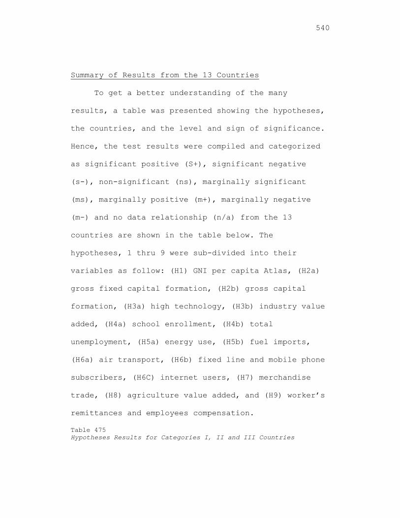
540

Summary of Results from the 13 Countries

To get a better understanding of the many

results, a table was presented showing the hypotheses,

the countries, and the level and sign of significance.

Hence, the test results were compiled and categorized

as significant positive (S+), significant negative

(s-), non-significant (ns), marginally significant

(ms), marginally positive (m+), marginally negative

(m-) and no data relationship (n/a) from the 13

countries are shown in the table below. The

hypotheses, 1 thru 9 were sub-divided into their

variables as follow: (H1) GNI per capita Atlas, (H2a)

gross fixed capital formation, (H2b) gross capital

formation, (H3a) high technology, (H3b) industry value

added, (H4a) school enrollment, (H4b) total

unemployment, (H5a) energy use, (H5b) fuel imports,

(H6a) air transport, (H6b) fixed line and mobile phone

subscribers, (H6C) internet users, (H7) merchandise

trade, (H8) agriculture value added, and (H9) worker’s

remittances and employees compensation.

Table 475 Hypotheses Results for Categories I, II and III Countries

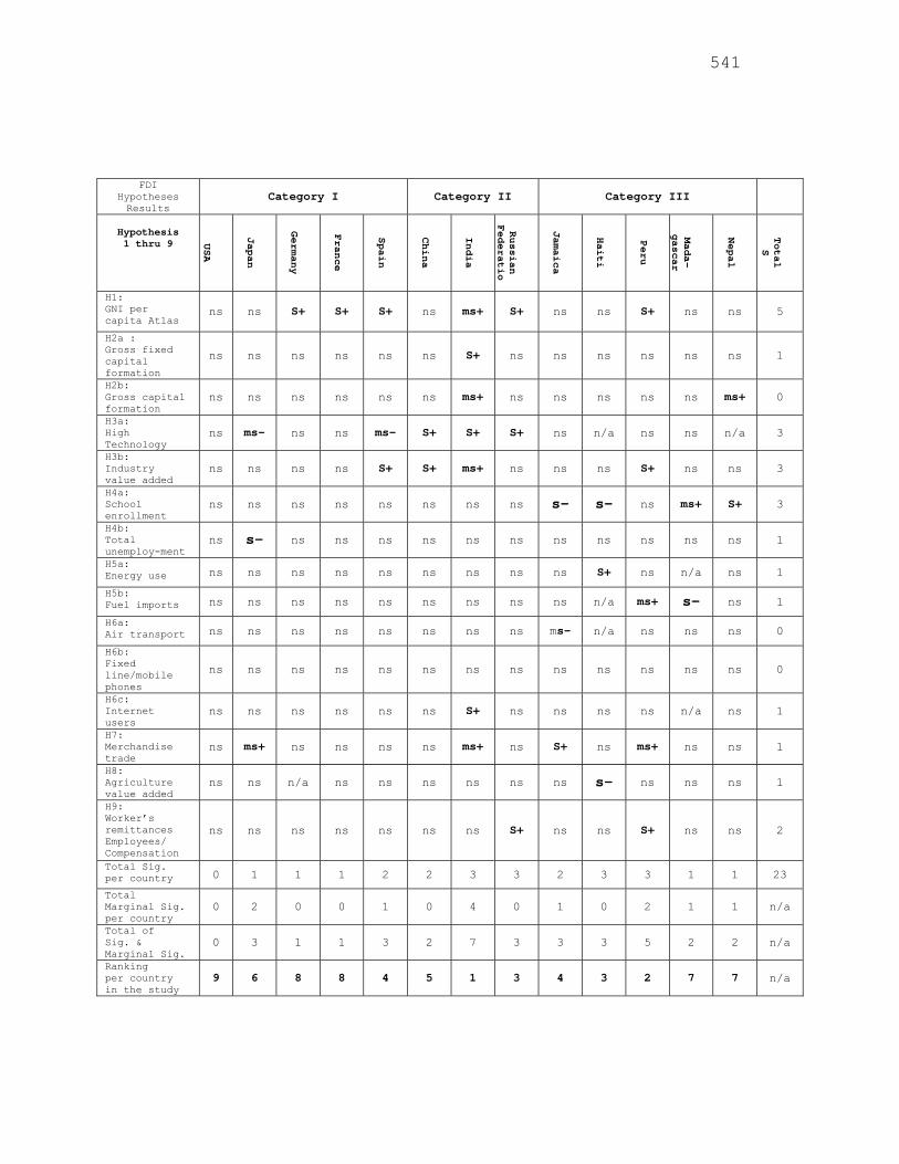
541

FDI

Hypotheses Results

Category I Category II Category III

Hypothesis 1 thru 9

USA

Japan

Germany

France

Spain

China

India

Russian

Federatio

Jamaica

Haiti

Peru

Mada-

gascar

Nepal

Total

S

H1: GNI per capita Atlas

ns ns S+ S+ S+ ns

ms+

S+ ns ns S+ ns ns 5

H2a : Gross fixed capital formation

ns ns ns ns ns ns S+ ns ns ns ns ns ns 1

H2b: Gross capital formation

ns ns ns ns ns ns ms+ ns ns ns ns ns ms+ 0

H3a: High Technology

ns ms- ns ns ms- S+ S+ S+ ns n/a ns ns n/a 3

H3b: Industry value added

ns ns ns ns S+ S+ ms+ ns ns ns S+ ns ns 3

H4a: School enrollment

ns ns ns ns ns ns ns ns s- s- ns ms+ S+ 3

H4b: Total unemploy-ment

ns s- ns ns ns ns ns ns ns ns ns ns ns 1

H5a: Energy use ns ns ns ns ns ns ns ns ns S+ ns n/a ns 1

H5b: Fuel imports ns ns ns ns ns ns ns ns ns n/a ms+ s- ns 1

H6a: Air transport ns ns ns ns ns ns ns ns ms- n/a ns ns ns 0

H6b: Fixed line/mobile phones

ns ns ns ns ns ns ns ns ns ns ns ns ns 0

H6c: Internet users

ns ns ns ns ns ns S+ ns ns ns ns n/a ns 1

H7: Merchandise trade

ns ms+ ns ns ns ns ms+ ns S+ ns ms+ ns ns 1

H8: Agriculture value added

ns ns n/a ns ns ns ns ns ns s- ns ns ns 1

H9: Worker’s remittances Employees/ Compensation

ns ns ns ns ns ns ns S+ ns ns S+ ns ns 2

Total Sig. per country 0 1 1 1 2 2 3 3 2 3 3 1 1 23

Total Marginal Sig. per country

0 2 0 0 1 0 4 0 1 0 2 1 1 n/a

Total of Sig. & Marginal Sig.

0 3 1 1 3 2 7 3 3 3 5 2 2 n/a

Ranking per country in the study

9 6 8 8 4 5 1 3 4 3 2 7 7 n/a

542

significant positive (S+), significant negative (s-), non-significant (ns), marginal (ms), marginally positive, (m+) marginally negative (m-) and no data relationships (n/a)

The empirical findings from Table 475 of

significant relationships (positive/negative) from the

testing of all hypotheses (1 thru 9) revealed that

India, the Russian Federation, Haiti and Peru had

three significant relationships per country, followed

by Spain, China and Jamaica totaling two significant

relationships per country. Japan, Germany, France,

Madagascar and Nepal had the least significant with

only one significant relationship per country. The

United States did not reveal any significant

relationship with the FDI to Cuba.

The three significant relationships corroborated

India’s and The Russian Federation’s involvement in

FDI investment with the Republic of Cuba. Surprising,

Haiti and Peru also revealed three significant

relationships; even though, these two countries did

not provide FDI to Cuba. Spain, China and Jamaica’s

two significant relationships with Cuba corroborated

the existing FDI investment these countries provided

543

to Cuba. Japan, Germany, France, Madagascar and Nepal

revealed one significant relationship with FDI to

Cuba. However, the result did not corroborate a

significant relationship for Madagascar and Nepal

since these two countries were not providing FDI to

Cuba. The result of the testing from the United States

did not have a significant relationship with FDI to

Cuba, justifying the effectiveness of the existing

trade embargo between the two countries.

When totaling the significant and marginal

relationships from Table 475 in order, India had the

the largest number (7) of relationships with FDI to

Cuba. Peru had the second greatest number (5) of

relationships with FDI to Cuba. Japan, Spain, The

Russian Federation, Jamaica and Haiti had the third

greatest number (3) of relationships with FDI to Cuba.

China, Madagascar and Nepal had the fourth greatest

number (2) of relationships with FDI to Cuba.

Germany and France had the fifth greatest number (1)

of relationships with FDI to Cuba. Lastly, the United

544

States had the sixth greatest number (0) (the least)

of relationships with FDI to Cuba.

As far as the three categories of the 13

countries, Category III countries had the most (Table

475, total significant/marginal significant)

significant number (15), followed by Category II

countries (12), and lastly Category I countries with a

significant number of (8) relationship with FDI to

Cuba.

In ranking (based on the number of significant

and marginally significant relationships), Category II

countries had the highest ranking with India (first),

the Russian Federation (third) and China (fifth). The

second highest ranking relationship was Category III

countries with Peru (second), Haiti (third), Jamaica

(fourth), Madagascar (seventh) and Nepal (seventh).

Lastly, Category I countries had the lowest ranking

with Spain (fourth), Japan (sixth), France (eighth),

Germany (eighth) and United States (ninth).

The key results of this study were as follows.

Technology in the other countries was a key variable

545

affecting FDI to Cuba. This was followed by the

variables, GNI per capita, and human capital

development in the countries studied. The other

variables showed up as significant for some countries

and not for others. Any variable that was not

significant for all countries? Category II countries

(China, India, and the Russian Federation) had the

highest number of significant and marginally

significant variables. This was followed by Category

III countries (Jamaica, Haiti, Peru, Madagascar and

Nepal) and Category I countries (United States, Japan,

Germany, France, and Spain).

Implication of the Study

A discussion of the significance of the variables

followed:

Level of technology was significant for 5 of the

13 countries. Hence, level of technology was a

significant variable affecting FDI to Cuba. Three of

these countries were from Asia (China, India and the

546

Russian Federation). Spain and Peru were also

significant. Japan, Spain and India was also

marginally significant. Hence, level of technology in

these countries had a significant impact on FDI to

Cuba.

GNI per capita was significant for 5 of the 13

countries. Hence, GNI per capita was a significant

variable affecting FDI to Cuba. Three of these

countries were from Europe (Germany, France, and

Spain). The Russian Federation and Peru were also

significant. India was marginally significant. Hence,

GNI per capita in these countries had a significant

impact on FDI to Cuba.

Human capital was significant for 4 of the 13

countries. Hence, human capital was a significant

variable affecting FDI to Cuba. Two of these countries

were from the Caribbean (Jamaica and Haiti). Japan and

Nepal were also significant. Madagascar was marginally

significant. Hence, human capital in these countries

had an impact on FDI to Cuba.

547

Energy and natural resources was significant for

2 of the 13 countries. These two countries were Haiti

and Madagascar. Peru was marginally significant.

Hence, energy and natural resources in these countries

did not have an impact on FDI to Cuba.

Governmental factor was significant for 2 of the

13 countries. Hence, governmental factors were not a

significant variable affecting FDI to Cuba. The only

two countries significant were the Russian Federation

and Peru. Hence, governmental factors did not have an

impact on FDI to Cuba.

Market type, referred to as the ability to create

marketing concept through FDI potentials and highly

competitive value chain as measured by merchandise

trade, was significant for 1 of the 13 countries.

Hence, market type was not a significant variable

affecting FDI to Cuba. The only country significant

was Jamaica. Japan, India and Peru were marginally

significant. Hence, market type in these countries did

not have an impact on FDI to Cuba.

548

Financial capital was significant for 1 of the 13

countries. That country was India. In addition, Nepal

and India showed marginally significance. Hence,

financial capital did not have a major impact on FDI

to Cuba.

Transportation and communication was significant

for 1 of the 13 countries. Hence, transportation and

communications was not a significant variable

affecting FDI to Cuba. The only country significant

was India. Jamaica was marginally significant. Hence,

transportation and communications in these countries

did not have an impact on FDI to Cuba.

Environmental factor was significant for 1 of the

13 countries. Hence, environmental factor was not a

significant variable affecting FDI to Cuba. The only

country significant was Haiti. Hence, environmental

factors did not have an impact on FDI to Cuba.

The findings from this study implied that policy

makers in these and other countries should look at the

key macro variables to evaluate the level of FDI

provided to Cuba and other developing countries. The

549

government of Cuba could also use these findings to

evaluate the key variables in other countries that

could affect FDI to Cuba. The government of Cuba could

also use the list of countries that were significant

as targets of promotion for FDI to Cuba. World

institutions, like World Bank and the International

Monetary Fund, could also use these results to try and

assist Cuba and other developing countries.

This was the first study that utilized a

macroeconomic approach to study FDI inflow to Cuba.

Hence, there was no comparative study.

Theoretical Implications

From the theoretical frameworks discussed in the

previous chapters, the major factor influencing a

nation’s international competitiveness was FDI

(Dunning, 1988). The dominant ‘eclectic paradigm’

(Dunning, 1988a) offers a more comprehensible reason

to set up production in a foreign country based on the

ownership, rival competition, and easy access to

operating in a foreign country. In Dunning’s theory

550

described in chapter 1 and further in chapter 2 made

it clear that once advantages of MC’s are established

those companies operating through FDI will branch out

with further operations in the same foreign locations

or in new ones (Letto-Gilles, 2002). The category II

countries, like China, India and most notably the

Russian Federation had established operations within

the Island of Cuba; in turn, expanding their

international production instead of their domestic

production. This supported Dunning’s (1980) ‘eclectic

theory,’ which explained the ability and willingness

of a firm to serve markets (local, domestic, or

international) and to exploit these advantages.

Dunning’s (1977, 1980) ‘eclectic theory’

explained that FDI firms were able to create vertical

and horizontal spillovers of technology and human

skills while expanding specialization of production.

This study showed that the level of technology in 5 of

the 13 countries affected FDI to Cuba. These

countries: were China, India, the Russian Federation,

Spain and Peru. In the case of the Russian

551

Federation, its long-term FDI interaction with Cuba

has created the necessary spillovers in the transfer

of technology, goods, resources, exports and FDI. The

Russian Federation not only had provided significant

FDI to Cuba, but had also provided intermediate goods,

services and large-scale production within the island;

thereby, creating locations advantages outside its

home country (Dunning, 1988b). These findings

supported Dunning’s ‘eclectic theory.’

Similar results were found for the level of

technology and FDI to China. Shi’s (2001) findings of

China’s technological transfer supported Dunning’s

(1988a) base theory regarding LSAs, which included

natural resources, cheap land and labor costs,

potential local markets and government policies.

The findings from Hypothesis 3, regarding the

level of technology for category II countries, China,

India and the Russian Federation, also supported

Hymer’s (1976) oligopolistic theory. Hymer (1976)

indicated that the driving force for firms to expand

abroad was the application of firm-specific skills or

552

technology to a wide market, not only to reallocate

the world’s capital. Furthermore, Hymer (1976)

mentioned that markets were highly imperfects for

firm-specific technology; therefore, a well-managed

local firms, drawing on their home court advantage,

would be able to obtain a greater return on good

technology than distant firms hovering in unfamiliar

territory (Hymer, 1976). For these particular reasons,

those MNCs that were successful would undoubtedly

penetrate and exploit their proprietary technology

(Hymer, 1976). In the case of China, India and the

Russian Federation, reiterating on Hymer (1976)

oligopolistic theory, by investing in Cuba and

providing FDI, MNCs from these host countries would

benefit from proprietary and good technology. This was

most notable in China, India and the Russian

Federation investment in Cuba’s off shore oil

exploration (Chloe, 2008)(Mesa-Lago, 2005) (Cuba

economy, 2008).

Hymer (1976) also stated that MNCs would provide

FDI along with technology to developing countries and

553

emerging markets. This study found that China, India

and the Russian Federation viewed Cuba as a viable

market for FDI.

Hypothesis 3, level of technology through Porter

(1980) three generic strategies further explained that

a firm used differentiation by citing to include

design or brand image, technology, features, customer

service, and dealer network.

Hypothesis 3, level of technology, through

Fosfuri and Motta (1999), also made reference for

firm-specific advantages to give rise to multinational

activity and provide a formal model of FDI would

result, in not exploiting existing technological

advantages in a foreign country, but to access such

technology and transfer it from the host economy to

the investing multinational corporation via spillover

effects (Love, 2003, p. 2).

Similar result of factors influencing FDI to Cuba

to human capital for hypothesis 4, which was

significant for 4 of the 13 countries. Dunning’s

‘eclectic theory’ improvised that the greatest

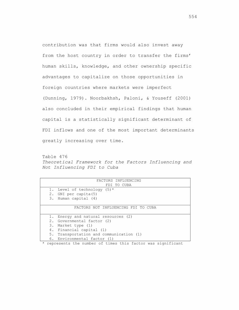
554

contribution was that firms would also invest away

from the host country in order to transfer the firms’

human skills, knowledge, and other ownership specific

advantages to capitalize on those opportunities in

foreign countries where markets were imperfect

(Dunning, 1979). Noorbakhsh, Paloni, & Youseff (2001)

also concluded in their empirical findings that human

capital is a statistically significant determinant of

FDI inflows and one of the most important determinants

greatly increasing over time.

Table 476 Theoretical Framework for the Factors Influencing and Not Influencing FDI to Cuba

FACTORS INFLUENCING FDI TO CUBA

1. Level of technology (5)* 2. GNI per capita(5) 3. Human capital (4)

FACTORS NOT INFLUENCING FDI TO CUBA

1. Energy and natural resources (2) 2. Governmental factor (2) 3. Market type (1) 4. Financial capital (1) 5. Transportation and communication (1) 6. Environmental factor (1)

* represents the number of times this factor was significant

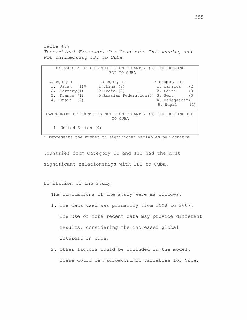
555

Table 477 Theoretical Framework for Countries Influencing and Not Influencing FDI to Cuba

CATEGORIES OF COUNTRIES SIGNIFICANTLY (S) INFLUENCING FDI TO CUBA

Category I Category II Category III 1. Japan (1)* 1.China (2) 1. Jamaica (2) 2. Germany(1) 2.India (3) 2. Haiti (3) 3. France (1) 3.Russian Federation(3) 3. Peru (3) 4. Spain (2) 4. Madagascar(1) 5. Nepal (1)

CATEGORIES OF COUNTRIES NOT SIGNIFICANTLY (S) INFLUENCING FDI

TO CUBA 1. United States (0)

* represents the number of significant variables per country

Countries from Category II and III had the most

significant relationships with FDI to Cuba.

Limitation of the Study

The limitations of the study were as follows:

1. The data used was primarily from 1998 to 2007.

The use of more recent data may provide different

results, considering the increased global

interest in Cuba.

2. Other factors could be included in the model.

These could be macroeconomic variables for Cuba,

556

including GDP, inflation rates, interest rates,

unemployment rates, income, and energy use, etc.

3. Some data were not available for a few countries

and affected four of the nine hypotheses.

4. The data from inside Cuba was limited and was

excluded from the testing. With more reliable

data from Cuba, the analysis could be expanded.

Future Research Recommendations

Several recommendations were suggested for future

research.

1. The time framework for future research could be

expanded prior to 1998 and/or beyond 2007,

2. More countries could be included, for example

Venezuela, Mexico, Canada, and Italy, etc.

3. More variables could be included in the study,

including inflation, energy imports, electricity

production, imports and exports, etc.

4. A bilateral approach could be studied. For example,

a study can be done to see the relationship between

FDI from Venezuela (Cuba’s largest trading partner)

557

and Cuba’s economy. Furthermore, a bilateral

approach with Cuba’s other existing trading partners

like Canada, Mexico and Italy and observed their

relationship between these countries economy and the

FDI to Cuba.

Summary

This chapter provided an explanation of the

results of the research. The findings of this study

described the nine hypotheses and their significant

relationships of macro variables in 13 countries and

FDI to Cuba. The study overwhelmingly determined that

FDI to Cuba was positively influenced by level of

technology, GNI per capita, and human capital in

several of the other countries. The study also

revealed that the macro variables for China, India and

the Russian Federation had the most influenced on FDI

to Cuba. Perhaps Cuba’s FDI would increase further if

the trade policies, particularly with the United

States, followed by Japan, Germany, France, Jamaica,

Haiti, Peru, Madagascar and Nepal were less

558

restrictive. Spain by itself had a significant

relationship, which corroborated the country´s long-

term trade and FDI to Cuba. None of the economic

variables from the United States was found to be

significant, implying the effectiveness of the trade

embargo to Cuba. However, the trade embargo is not the

primary factor for Cuba deteriorating economic

condition. Cuba’s centrally planned system with

limited government reforms and its inappropriate labor

incentive has been the leading cause for Cuba’s

diminishing economy (Pellet, 1976, 1986). In any case,

even with the United States economic embargo, FDI to

Cuba was impacted by economic activities in other

countries.

559

BIBLIOGRAPHY

Adler, M., & Hufbauer, G. C. (2008). Policy

liberalization and FDI growth, 1982 to 2006. Washington, DC: Peterson Institute for International Economics, Allen, F., & Gale, D. (1999). Corporate governance and competition. Working Paper, University of Pennsylvania. August, R. (2004). International business law, Text, Cases, and readings (4th ed.). Upper Saddle River, NJ: Pearson Prentice Hall.

Babbie, S. A. (2001). The practice of social research (9th ed.). Belmont, CA: Thomson Learning, Inc.

Band, W. (1995). Customer-accelerated change.

Marketing Management, 4(3), 18-309. Balcerovicz, L., Blaszczyk,B. & Dabrowski, M. (1997). The Polish way to the market economy, in J. Sachs (Ed.) Economies in Transition. Cambridge, MA: MIT Press. Ball, D., McCulloch, W. H., Frantz, P. L., Geringer, J. M., & Minor, M. (2002). International business: The challenge of global competition (8th ed.). NY: McGraw-Hill Companies.

Bennett, D., Liu, X. M., Parker, D., Steward, F., & Vaidya, K. (2001). Technology transfer to China: A study of strategy in 20 EU Industrial Companies. International Journal of Technology Management, 21(1-2), 151-182.

Bers, J. A., Lynn, G. S., & Spurling, C. (1997).

A venerable tool for a new application: Using scenario

560

analysis for formulating strategies for emerging technologies in emerging markets. Engineering Management Journal, 9(2), 33-40.

Birnbaum, J. (2002). Business to Bush: Let us into Cuba. Fortune Magazine, 45(11), 36.

Blau, G., Boal, J., & Kimberly, B. (1987).

Conceptualizing how job involvement and organizational commitment affect turnover and absenteeism. Academy of Management Review, 12(2), 288-300.

Blomstrom, M., & Sjoholm, F. (1999). Technology transfer and spillovers: Does local participation with multinationals matter? European Economic Review, 43(4-6), 915-923.

Brightman, H., & Schneider, H. (1994). Statistics

for business problem solving (2nd ed.). Cincinnati, OH: South Western Publishing Company. Caldwell, R. J. (2002, April 21). A failed revolution leaves Cuban poor, oppressed. San Diego Union Tribune. Calzon, F. (2002). Will subsidized trade with Cuba help the American Farmer or hurt the United States taxpayers? Washington: Center for a Free Cuba. Cantwell, J., & Narula, J. (2003). International business and eclectic paradigm: developing the OLI framework. Journal of International Business Studies 35, 456-458.

Carter, T. (1997, December 15). Are sanctions really working? Some dispute effectiveness in foreign policy. The Washington Times, 1-4. Castro, F. (2004b). Buenas noticias para finalizar el ano. Granma, December 25, 2004.

561

Caves, R. E. (1971). International corporations: The industrial economics of foreign investment. Economics, 38, 1-27. Chen, E. (2002, May 20). The world: Bush to extend hand to Cubans’ policy. The Los Angeles Times, p. A.1.

Chen, T. J., & Ku, Y. H. (2000). The effects of foreign direct investment on firm growth: The case of Taiwan manufacturers. Japan and World Economy, 12(2), 153-172, Taiwan. Chiou, J. R., Wang, M. L., & Wu, J. J. (2001). Effects of capital utilization and industry difference on FDI performance-Taiwanese firms in mainland China, Singapore, Malaysia, and Thailand. Issues & Studies. 37(6), 59-76. Chloe, Hayward (2008, November). Cuba’s Capitalist Evolution. Euromoney, 39(1), 84-87. Clinton, W. J. (1995, April 14). Interview with Wolf Blitzer and Judy Woodruff on CNN. Weekly Compilation of Presidential Documents, 31, 624-625.

Cruz, R. D. (2003). Foreign direct investment in post Castro Cuba: Problem, opportunities and recommendations. Miami Florida: University of Miami, Institute for Cuban and Cuban American Studies.

Cuba economy: Foreign investment is

growing. (2008, August). EIU ViewsWire. Retrieved November 26, 2009, from ABI/INFORM Global. (Document ID: 1547335981).

Cuba: Hurricane damage fuels policy pressure.

(2008, September 25). Oxford Analytica Daily Brief Service, p. 1.

562

Deichmann, J. I. (2004). Origins of foreign direct investment in Poland, 1989-2001. The Journal of Business and Economic Studies, 10(1), 1-13.

Dianchun, J., Jinghan, J., & Isaac, D. (1998). The effect of foreign investment on the real estate industry in China. Urban Studies, 35(11), 2101-2111. Dolan, K. (1998). Give ‘em rope. Forbes Magazine, 162(13), 218.

Drabek, Z., & Warren, P. (1999). The impact of transparency on foreign direct investment. Staff Working Paper ERAD-99-02, Geneva, World Trade Organizations.

Dunne, N. (1997, September 15). The United States companies plan attack on sanctions-lobby group claims markets are being lost. Financial Times.

Dunning, J. H. (1977). Trade location of economic

activities and the MNE: A search for an eclectic approach. London: Macmillian.

Dunning, J. H. (1979). Explaining changing

patterns of international production: In defense of the eclectic theory. Oxford Bulletin of Economics and Statistics, 41, 269-295.

Dunning, J. H. (1980). Explaining changing

patterns of international production: in defense of the eclectic theory Oxford Bulletin of Economics and Statistics, 41(4), 269-295.

Dunning, J. H. (1980). Toward an eclectic theory

of international production: Some empirical tests. Journal of International Business Studies, 11(1), 9-31.

Dunning, J.H. (1981a) Explaining outward direct

investment of developing countries: In support of the eclectic theory of international production. In K.

563

Kumar & M.G. McLeod (eds.), Multinationals from Developing Countries. Washington: Heath. Dunning, J. (1988a). Explaining international production. London: Unwin Hyman. Dunning, J. H. (1988b). The eclectic paradigm of international production: a restatement of and some possible extension. Journal of International Business Studies, 19, 1-31. Dunning, J. (1988b). The eclectic paradigm of international production: A restatement and some possible extension. Journal of International Business Studies, 19(1), 1-31. Dunning, J. H. (1992). The global economy, domestic governance, strategies and transnational corporations: Interactions and policy implications. Transnational Corporations, 1(3), 7-44.

Dunning, J. H. (1993). Multinational enterprises and the global economy. Reading, MA: Addison-Wesley Publishing Company.

Dunning, J. H. (1994). Re-evaluating the benefits

of foreign direct investment. Transnational Corporations, 3, 23-51.

Dunning, J. (1995). Reappraising the eclectic

paradigm in an age of alliance capitalism. Journal of International Business Studies, 26(3), 461-491.

Dunning, J. H. (1995). Multinational enterprises

and the global economy. Wokingham, UK: Addison-Wesley. Dunning, J. H. (1998). Location and the

multinational enterprise: A neglected factor? Journal of International Business Studies, 29(1), 45-66.

Dunning, J. H. (2000). The eclectic paradigm of

international production: A personal perspective, The

564

Nature of the Transnational Firm (2nd ed.). London: Routledge.

Dunning, J. (2003). The moral response to

capitalism: Can we learn from the Victorians? in J. Birknshaw, S. Ghoshal, C. Markides, J. Stopford & G. Yip (eds). The Future of the Multinational Company (pp. 14-33). Chichester: Wiley.

Economic Commission for Latin America and the

Caribbean (ECLAC). (2004c). Preliminary overview of the economies of Latin America and the Caribbean. Santiago de Cuba: ECLAC. Energy Information Administration (EIA). (2006). Official energy statistics from the United States’ government. Retrieved July 21, 2009, from www.eia.doe.gov

Engle, J. (2002, September 1). Travel Americans abroad tourism: Cuba sanctions. Los Angeles Times, p. L.2. Fabry, N., & Zeghni, S. (2002). Foreign direct investment in Russia: How the investment climate matters. Communist and Post Communist Studies, 35(3), 289-303. Fahy,J., Hooley, G., Berca, J., Fonfara, K., & Gabrijan, V. (2003). Privatization and sustainable Competitive advantage in the emerging economies of Central Europe. Management of International Review, Weisbaden, 43(4), 1-14. Firth, M., Fung, P., Rui, M. Y., & Oliver, M. (2005, March 24). Corporate performance and CEO compensation in China. Journal of Corporate Finance, 1-32. Font, M. A. (1996). Friendly prodding and other sources of change in Cuba Social Research. NY: Proquest NOVA Southeastern University.

565

Fontova, H. (2008, February 25). What’s next for Cuba? Human Events Publishing, 64(7), 1-8. Foreign and Direct and Investment. (2001). Trade and commerce. NY: Institute for Cuban-American Studies. Fosfuri, A., & Motta, M. (1999). Multinationals without advantages. Scandinavian Journal of Economic, 101, 617-630. Frankel, J. (1997). Regional trading blocs in the world economic system. Washington: Institute for International Economics. Freedom House. (2001). Freedom in the world 2000-2001. NY: Freedom House. Fuat, E., & Ekrem, T. (2002). Locational determinants of foreign direct investment in an emerging market economy: Evidence from Turkey. Multinational Business Review, 10(1), 7-21. Globerman, S., & Shapiro, D. (2003). Governance infrastructure and the United States foreign direct investment. Journal of International Business Studies, 34(1), 19-39. Graham, E. M. (2000). Subsides, market closure, cross-border investment, and effects on competition: The case of FDI in the telecommunications sector. Institute for International Economics, 29(1), 1-24. Graham, E. M., & Krugman, P. R. (1995). Foreign direct investment in the United States, (3rd ed.). Washington: Institute for International Economics. Groose, R. E. (1980). Foreign investment codes and the location of direct foreign investment. NY: Praeger.

566

Groves, T., Hong, Y., McMillan, J., & Naughton, B. (1994). Autonomy and incentives in Chinese state enterprises. Quarterly Journal of Economics, 109, 183-209. Groves, T., Hong, Y., McMillan, J., & Naughton, B. (1995). China’s evolving managerial labor market, Journal of Political Economy, 103, 873-892.

Gutierrez, T. (1966, July 25). U.S. vs Cuba: Helm-Burton Act arouses worldwide anger. Via Workers World News Service, 1-16.

Habib, M., & Zurawicki, L. (2002). Corruption and foreign direct investment. Journal of International Business Studies, 33(2), 1-28.

Harvard College Library. (2009). Foreign direct

investment data resources. Retrieved August 31, 2009, from http://hcl.harvard.edu/research/guides/fdi/

Havana Journal. (2006, March 14). Cuba to work on

Ethanol production. Retrieved August 21, 2009, from http//economictimes.Indiatimes.com

Havana Journal.(2006, Nov 20). State of Cuban oil

exploration and development of sugar ethanol industry. Cuba Business. http//economictimes.Indiatimes.com

Havana Journal. (2008, May 18). Cuba trade

delegation to India looking for trade and credit line. Retrieved August 21, 2009, from http//economictimes.Indiatimes.com

Hayek, H. F. A. (1935). Prices and production.

London: Routledge, George, and Keegan, Paul. Hickling-Hudson, A. H. (2004). South-south

collaboration, Cuban teachers in Jamaica and Namibia. Queensland University of Technology, 40(2).

567

Hymer, S. H. (1970). The efficiency (contradictions) of multinational corporations. American Economic Review, LX(2), 441-448. Hymer, S. H. (1976). The international operations of national firms: A study of direct foreign investment. Cambridge, MA: MIT Press. Hodgetts, R. M., & Luthans, F. (2000). International management, culture, strategy and behavior (4th ed.). NY: Irwin McGraw-Hill. Inside the United States trade. (1992). Washington, DC: United States Information Service (USIS). Institute for Cuban & Cuban-American Studies. (2001). Cuba on-line. Coral Gables, FLA: University of Miami. Institute for Cuban & Cuban-American Studies. (2002). Cuba on-line. A comparative look at socio-economic Conditions in pre-Castro Cuba and present day Cuba. Coral Gables, FLA: Bureau of Inter-American Affairs, Department of State, University of Miami. Jacoby, J. (2001, June 21). Cuban liberty and a test for Bush. Boston Globe, p. A.15. Jamaica sees Cuba in planned free-trade area (5th ed.). (1998, December 14). Journal of Commerce, p. 8. Retrieved December 3, 2009, from ABI/INFORM Global. (Document ID: 37104004). Jiang, D., Jinghan, J., & Isaac, D. (1998). The effect of foreign direct investment on the real estate industry in China. Urban Studies Edinburgh, 35(11), 1-9. Jonquieres, G. (1997, July 31). Keeping the lid on Helms-Burton: The United States and EU warn that talks may prove complicated. The Financial Times, 4.

568

Kaufmann, D., Kraay, A., & Zoido-Lobaton, P. (1999). Aggregating governance indicators. World Bank, Working Paper no. 2195. Katzer, J., Cook, K. H., & Crouch, W. W. (1998). Evaluating information: A guide for users of social science research (4th ed). NY: McGraw-Hill.

Kindleberger, C. P. (1969). American businesses abroad: Six lectures on direct foreign investment. New Haven, NJ: Yale University Press.

Kobrin, S. (1976). The environmental determinants

of foreign direct manufacturing investment: An export empirical analysis. Journal of International Business Studies, 7(1), 29-42.

Kogut, B., & Singh, H. (1988). The effect of national culture on the choice of entry mode. Journal of International Business Studies, 19, 411-32.

Kotler, P. (1967). Marketing management:

Analysis, planning and control. Englewood Cliffs, NJ: Prentice Halls.

Kotler, P. (1971). Marketing decision making: A

model building approach. NY: Rinehart and Winston. Kotler, P. (1972b). What consumerism means for

marketers. Harvard Business Review, 50, 48-57. Kotler, Philip (1975). Marketing for Nonprofit

organizations. Englewood Cliffs, New Jersey: Prentice-Hall.

Kotler, P. (1986b). Megamarketing. Harvard

Business Review, 64, 117-124. Kotler, P. (1997a). The Marketing of nations: Somkid Jatusripitak and Suvit Maesincee. NY: Free Press.

569

Kotler, P. (1997b). Marketing management. Planning, analysis, and control, (9th ed.). Englewood Cliffs, NJ: Prentice Hall. Kotler, P. (1999). Kotler on marketing: How to create, win and dominate markets. NY: Free Press. Krugman, P.R., Obstfeld, M.(2009). International Economics, theory and policy, (8th ed.). MA: Addison-Wesley. Kuester, S., Homburg, C., & Robertson, T. S. (1999). Retaliatory behavior to new product entry. Journal of Marketing, 63(4), 90-106.

Lall, P. , Norman. W. D., & Featherstone, A. M. (2003). Determinants of the United States direct foreign investment in the Caribbean. Applied Economics, Business & Company Resource Center, 35(13), 1-23. Law, K. S., Tse, D. K., & Zhou, N. (2003). Does human resource management matter in a transitional economy? China as an example. Journal of International Business Studies, 34(3), 255.

Leedy, P. D., & Ormrod, J. E. (2004). Practical research, planning and design (8th ed.). NY: Prentice-Hall. Letto-Gilles, G. (2002). Hymer, the nation-state and the determinants of multinational corporations’ activities. Contributions to Political Economy, Oxford, 21(1), 43. Li, W. (1997). The impact of economic reforms on the performance of Chinese state enterprises, 1980-1989. Journal of Political Economy, 105, 1080-1106. Liu, X. (1995). Zhongguo, Duiwai, Jingji, Maoyi, Zhengce, Zhinan (Guidebook of China Foreign Economic

570

and Trade Policies). Beijing: China Economic Management Press. Love, J. H. (2003) Technology sourcing versus technology exploitation: An analysis of the United States foreign direct investment flows. Journal of Applied Economics, 35(15), 1167-1179. Lucom, W. C. (2004, July 19). Castro’s socialism fails workers. Investor’s Business Daily, 1-2. Luo, Y. (2001). Market-seeking MNEs in an emerging market: How parent-subsidiary links shape overseas success. Journal of International Business Studies, 34, 290-309. Mack, S. K. (2002, December 20). Maine sees potential for trade with Cuba state delegation: Castro discuss food export. Bangor Daily News, 1-5. Maddison, Angus (2003). Development centre studies. The World Economy Historical Statistics. USA. OECD Publishing, 144-150. Marx, G., & Witt,H. (2002, April 26). Cuba market tempts merchants; U.S. businesses see potential for sales. Chicago Tribune, 1-6. McPherson, M. Q. T. (2007, July). What if Cuban trade was based on economic fundamentals instead of political policies? An estimate of Cuba’s trade distortion. Cuban Affairs Quarterly Electronic Journal, 2(3). Mesa-Lago, C. (1979). Dialectica de la Revolucion Cubana:del idealismo carismatico al pragmatismo institucionalista. Madrid, Spain: Biblioteca Cubana Contemporanea. Mesa-Lago, C. (2001). The Cuban economy at the start of the 21st Century: The Cuban Economy in 1999-

571

2001: Evaluation of Performance and Debate on the Future. Cuba in Transition, 11, 1-15. Mesa-Lago, C. (2005). The Cuban economy today: Salvation or damnation? Coral Gables, FLA: Institute for Cuban and American Studies, University of Miami. Michalak, W. (1993). Foreign direct investment and joint ventures in East Central Europe: A geographical perspective. Environment and Planning, 25, 1573-1591. Miles, R. E., & Snow, C. C. (1978). Organizational strategy, Structure, and process. NY: McGraw-Hill. Molina, C. D., & Valdesfully, M. C. (2000). Reflecting on the successes, problems and challenges of psychology. Revista Interamericana de Psicologia, 34(2), 169-183.

Molina-Lacayo, L.I. (2003). Study of Foreign Direct Investment in Manufacturing vs. Service Industries: “A Nicaraguan Perspective.” MI: Proquest. Motta, M., & Norman, G. (1996). Does economic integration cause foreign direct investment? International Economic Review, 37(4), 757-775. Newburry, W., & Yakova, N. (2003). Standardization preferences: A function of national culture, work interdependence and local embeddedness. Journal of International Business Studies, 37, 44-60. Nickels, W., McHugh, J. M., & McHugh, S. M. (2005). Understanding business: Competing in global markets (7th ed.). NY: McGraw-Hill Irwin. Ning, Y., & Reed, M. R. (1995). Locational determinants of the United States direct foreign investment in food and kindred products. Agribusiness: An International Journal, 11, 77-85.

572

Noorbakhsh, F., Paloni, A., & Youseff, A. (2001). Human-capital and FDI inflows to developing countries-New empirical evidence. World Development, 29(9), 1593-1610.

Ohlin, B. (1933). Interregional and international trade. Boston: Harvard University Press. Pearce II, J. A., & Robinson Jr., R. B. (2003). Strategic management: Formulation, implementation and control (8th ed.). NY: McGraw-Hill Irwin. Pellet, P.F. (1976). The System of Labor Incentives in the Cuban Economy from 1950 to 1970. University of Puerto Rico, Puerto Rico. Pellet, P.F. (1986). Socio-Economic Models and the Impacts of a Small Socialist Economy on an Industrialized Society: The Cases of Cuba and the USSR in Historical Perspective. University of Miami, Miami, Fl. Porter, M. E. (1980). Competitive strategy. NY: The Free Press. Porter, M. E. (1996). What is strategy? Harvard Business Review, 61-78.

Porter, M. E. (2001). Strategy and the Internet. Harvard Business Review, 63-78.

Provocative insight from the marketing guru.

(1999, July 25). The Jakarta Post, 1-2.

Qiu, L. D., & Tao, Z. G. (2001). Export, foreign direct investment, and local content requirement. Journal of Development Economics, 66(1), 101-125.

Rangan, K. V., Menenzes, M. A. J., Maier, E.P.

(1992, July). Channel Selection for New Industrial

573

Products: A Framework, Method, and Application. Journal of Marketing, 56(3), 69-82. Rodriguez, J. L. (2004). Informe a la Asamblea Nacional sobre los resultados economicos de 2004 y el plan economico social para 2005. Havana, AN. Sawalha, N. N. (2007). The role of the multinational corporations in economic development for countries with limited resources. NY: Proquest. Sethi, D., Guisinger, S. E., Phelan, S. E. & Berg, D. M. (2003). Trends in foreign direct investment flows: A theoretical and empirical analysis. Journal of International Business Studies. 34(4), 315. Sheth, J. N. (1974). A field study of attitude structure and the attitude behavior relationship in models of buyer behavior: Conceptual, quantitative, and empirical. NY: Harper & Row Publishers. Sheth, J. N., Gardner, D. M., & Garrett, D. E. (1988). Marketing theory: Evolution and evaluation. NY: John Wiley & Sons. Sheth, J. N., & Wright, P. (Eds.). (1974). Marketing analysis for societal problems. Urbuna-Champaign: Bureau of Economics and Business Research, College of Commerce and Business Administration, University of Illinois. Shi, Y. (2001). Technological capabilities and international production strategy of firms: The Case of foreign direct investment in China. Journal of World Business, 36(2), 1-28. Shirley, M., & Xu, L. C. (1998). Information, incentives, and commitment: An empirical analysis of contrasts between governments and state enterprises. Journal of Law, Economics, and Organization, 14, 358-378.

574

Siripaisalpipat, P. , & Hoshino, Y. (2000). Firms specific advantages, entry modes, and performance of Japanese FDI in Thailand. Japan and the World Economy, 12(1), 33-48. Smith, N., & Rebne, D. ( 1992). Foreign direct investment in Poland, the Czech and Slovak Republics and Hungary: The Centrality of the joint venture entry mode. The Mid-Atlantic Journal of Business, South Orange, 28(3), 1-23.

Sneed, M. (2002, January 25). Ryan invites Castro: Urges embargo end. Chicago Sun Times, 1-3. Snowdon, B., & Stonehouse, G. (2006). Competitiveness in a globalize world: Michael Porter on the microeconomic foundations of the competitiveness of nations, regions, and firms. Journal of International Business, 37, 163-175. Suarez, E. M. (1996). The Caribbean in transition, in choice and changes: Reflections on the Caribbean. NY: John Hopkins University Press. Sun, Q., & Tong, W. H. S. (2003). China share issue privatization: The extent of its success, Journal of Financial Economics, 70(2), 183-222. Tanzi, V. (1998). Corruption around the world: Causes, consequences, scope, and cures. IMF Working Paper WP/98/63, International Monetary Fund, Washington, D.C.

Terzian, P. (2001). Commentary- Havana, then and now. Providence Journal, Providence, RI.

The never-ending Cuban embargo. (2002, May 17).

Wall Street Journal, p. A.11.

575

Thomas, S. (1993). The politics and economics of privatization in Central and Eastern Europe. Columbia Journal of World Business, 28, 169-178.

Travieso-Diaz, M., & Trumbull, C. (2003). Foreign

investment in Cuba: Prospects and perils. The Washington International Law Review, 35(4), 903.

UNCTAD. (2001). World investment report:

Promoting linkages. NY: United Nations. UNCTAD. (2008). World investment report:

Promoting linkages. NY: United Nations. United States Congress, Committee of Conference.

(1996). Cuban liberty and democratic solidarity (Libertad) Act of 1996. Report 104-468, 104th Congress, 2nd Session, March 1, 1996, p. 66.

United States companies pay penalties for trade

with certain nations. (2002, July 3). New York Times, p. A9.

United States Department of State. (2003). Cuba:

Economic summary. Retrieved July 14, 2009, from http://www.state.gov/p/wha/rls/fs/22902.htm

USDA International Agricultural Trade

Report.(2002, August 5) Dairy Livestock & Poultry Trade Update. USA. Urquhart, J. (1997, March 14). Walmart puts Cuban goods back on sale. Wall Street Journal, p. A.3.

US out of step with Cuba embargo bill (2000, October 24). Evening Post, p. 1-3. Vanderbush, W., & Haney, P. J. (2002). Clinton, Congress, and Cuba policy between to codifications: The changing executive-legislative relationship in foreign policy making. Congress & the Presidency, 29(2), 169-194.

576

Varouj, A. A., Ying, G., & Jiaping, Q. (2005). Can corporations improve the performance of state-owned enterprises even without privatization? Journal of Corporate Finance, 11(5), 1-25. Vernon, R. (1966). International investment and international trade in the product cycle. Quarterly Journal of Economics, LXXX, 190-207. Vicker, J., & Yarrow, G. (1991). Economic perspectives on privatization. Journal of Economic Perspectives, 5, 111-132.

Vliert de Van, E. (2003, January). Thermoclimate, culture, and poverty as country-level roots of workers’ wages. Journal of International Business Studies, 34(1), 40-53. Wall Street Journal. (1982, September 2). Cuba’s inability to repay principal debt. p. 1. Wei, H. (1997). An examination of strategic foreign direct investment decision processes: The case of Taiwanese Manufacturing SME’s. Management Decision, 35(8), 619-630. Wei, Z., Varela, O., D’Souza, J., Hassen, M. K. (2003, Summer). The financial and operating performance of China’s newly privatized firms. Financial Management, 32(2), 126-197. Weinstein, A. & Johnson, W. C. (1999). Designing and delivering superior Customer value, concepts, cases, and applications. NY: CRC Press.

Wierenga, B., & Van Bruggen, G. H. (1997, July). The integration of marketing problem-solving modes and marketing management support systems. Journal of Marketing, 61(3), 21-37. Williams, C. J. (2003, January 2). Economic conditions foreign policy-United States-The United

577

States embargoes & blockades. Los Angeles Times, p. A1. WIR. (2001). World investment report. Geneva, Switzerland: United Nations.

Witt, H. (2003, April 29). US weighs new sanctions on Cuba. Chicago Tribune, p. 1.1. Wooster, R. B. (2003). The United States companies in transition economies: Wealth effects from expansion between 1987 and 1999. Journal of International Business, 37, 179-195. Wright, P. L. (1973). Use of consumer judgement models in promotion planning. Journal of Marketing, 37, 27-33. Yadoung, L., & Peng, M. W. (1999). Learning to compete in a transition economy: Experience, environment, and performance. Journal of International Business Studies, 30(2), 269. Yarrow, G. (1986). Privatization in theory and practice. Economic Policy, 2, 324-364. Young, S., & Lan, P. (1997). Technology transfer to China through Foreign Direct Investment. Regional Studies Cambridge, 31(7), 1-13.

Zenith and Eclipse: A comparative look at Socio-Economic condition in pre-Castro and present day Cuba. (1998). Bureau of Inter-American Affairs, 1-5. Zhang, D. D. (1998). The Case of Japanese FDI in China. Pacific Review, 11(1), 51-78.