Solar Phys (2015) 290:2409–2422DOI 10.1007/s11207-015-0705-0

R A D I O H E L I O P H Y S I C S : S C I E N C E A N D F O R E C A S T I N G

A Low-Frequency Radio Spectropolarimeterfor Observations of the Solar Corona

P. Kishore1 · R. Ramesh1 · C. Kathiravan1 ·M. Rajalingam1

Received: 17 October 2014 / Accepted: 18 May 2015 / Published online: 8 July 2015© Springer Science+Business Media Dordrecht 2015

Abstract A new spectropolarimeter for dedicated ground-based observations of radio emis-sion from the solar corona at low frequencies (<100 MHz) has recently been commissionedat the Gauribidanur Radio Observatory near Bengaluru, India. We report the observationalsetup, the calibration scheme, and first results.

Keywords Instrumentation and data management · Sun · Flares · Corona · Magnetic field ·Polarized radio bursts

1. Introduction

Direct estimates of the magnetic-field strength [B] in the solar atmosphere are currentlylimited to the inner corona, i.e. to a radial distance r � 1.2 R� (Kuhn and Penn, 1995; Lin,Kuhn, and Coulter, 2004; Gelfreikh, 2004; White, 2005). In the outer corona, i.e. r � 3 R�,Faraday rotation observations of microwave signals emitted by transmitters onboard artifi-cial satellites and/or distant background cosmic sources that pass through the solar coronaare used to derive the magnetic-field strength (Pätzold et al., 1987; Spangler, 2005). Com-pared to this, polarization measurements in the range 1.2 R� � r � 3 R� (i.e. middle corona)are rare due to lack of observational facilities. As the photosphere, chromosphere, andcorona are coupled by the solar magnetic field, the magnetic-field strength in this distancerange is generally obtained by mathematical extrapolation of the observed line-of-sight com-ponent of the photospheric magnetic field assuming a potential or force-free model (Schat-ten, Wilcox, and Norman, 1969; Schrijver and Derosa, 2003). Most of the low-frequencysolar radio bursts originate in the middle corona, and their emission mechanism is due toplasma processes (McLean, 1985). Plasma emission in the presence of a magnetic field issplit into ordinary [O] and extraordinary [X] modes. As a result of the differential absorp-

Radio Heliophysics: Science and ForecastingGuest Editors: Mario M. Bisi, Bernard V. Jackson, and J. Americo Gonzalez-Esparza

B P. Kishorekishore@iiap.res.in

1 Indian Institute of Astrophysics, II Block Koramangala, Bengaluru 560 034, India

2410 P. Kishore et al.

tion of these two modes in the medium, a net degree of circular polarization (dcp) can beobserved (Melrose and Sy, 1972). The latter is related to the strength of the magnetic field inthe source. This enables estimating the coronal magnetic-field strength using observationsof polarized radio bursts (Dulk and McLean, 1978; Mercier, 1990; Ramesh et al., 2003;Ramesh, Kathiravan, and Satya Narayanan, 2011; Sasikumar Raja and Ramesh, 2013; Har-iharan et al., 2014). Note that due to the decrease in the coronal electron density [Ne] andhence the associated plasma frequency [fp] with increasing height in the solar atmosphere,the lower the observation frequency, the larger the corresponding radial distance. This makesobservations with a broadband radio spectropolarimeter useful because the field strengthcan be obtained over a range of r for the same event in a near-simultaneous manner. TheIndian Institute of Astrophysics (IIA) has recently commissioned a radio spectropolarimeterfor dedicated observations of the solar corona in the frequency range 85 – 35 MHz at theGauribidanur Observatory [www.iiap.res.in/centers/radio]. Radio emission in this frequencyrange typically originates in the range 1.2 R� � r � 2 R� in the solar atmosphere. This arti-cle describes the observational set-up, calibration schema, and first results on the estimatesof the coronal magnetic-field strength in this distance range.

2. Observational Setup

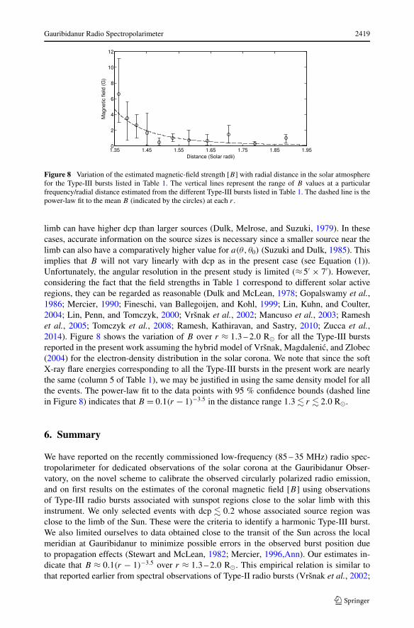
The front-end of the radio spectropolarimeter (Gauribidanur RAdio SpectroPolarimeter:GRASP) consists of two log-periodic dipole antennas (LPDAs: Carrel, 1961; Ramesh et al.,1998; Kishore et al., 2014) designed and fabricated at the Gauribidanur Observatory forobservations in the frequency range of 85 – 35 MHz with VSWR � 2 and directional gainof ≈7 dBi (with respect to an isotropic antenna). The effective collecting area [Ae] of eachLPDA is ≈0.4λ2, where λ is the observation wavelength. Figure 1 shows the block dia-gram of the GRASP set-up. The LPDAs have been mounted vertically with a spacing [d] often meters between them in the north–south direction. While the orientation of the “arms”in one of the LPDAs is east–west, they are in the north–south direction for the other, i.e.the two LPDAs are mutually perpendicular (Figure 2). The LPDAs respond to a linearlypolarized signal in the direction of the orientation of their arms. The half-power width ofthe response pattern (beam) of the two LPDAs is ≈80◦ in the E-plane and ≈110◦ in theH-plane, independent of frequency. This enables us to carry out observations for a longertime duration (� six hours) and over a wide range of declinations. We note that although thenorth–south oriented baseline between the two LPDAs facilitates observations without theneed for steering the beam of the LPDAs along the hour angle, there will be a delay d sin θ ,where θ is the zenith angle, between the RF signal incident on the two LPDAs dependingon the declination of the radio source. This will lead to phase difference, a function of fre-quency, between the two signals. We have provision to include coaxial cable of appropriatelength in the signal path from either of the two LPDAs to compensate for this delay. We notethat this delay is nearly constant over a ≈ ± three-hour observing period in hour angle fora particular declination. Moreover, since the change per day in the declination of the Sun isminimal (≈0.1◦), inclusion of a co-axial cable of specific length will provide the requireddelay for about one month. The residual phase difference is �±5◦ over the 85 – 35 MHzband.

The radio frequency (RF) signals from individual LPDAs are high-pass filtered and am-plified by ≈28 dB in the first-stage amplifier. After transmission over a distance of ≈20 mvia a coaxial cable, the signals are again amplified by ≈30 dB in a second-stage amplifier.

Gauribidanur Radio Spectropolarimeter 2411

Figure 1 Block diagram of theGRASP.

Figure 2 A view of the GRASP. While the two nearby LPDAs in mutually orthogonal orientation (tenmeters) are part of the GRASP, the third antenna belongs to the e-CALLISTO set-up at the observatory (Benzet al., 2009). The white enclosures (height ≈ 1.2 m) near each antenna houses the respective RF-to-opticalconverters.

2412 P. Kishore et al.

The signal amplitude after these two stages of amplification is ≈−40 dBm in each pathand is nearly constant over the entire RF band (85 – 35 MHz) to within ±1 dB. The ampli-fied RF signal from the two antennas is independently converted into an optical signal bymodulating with a low-power laser (+4.5 dBm at 1310 ± 10 nm) in two separate RF-to-optical converters. The maximum RF input power that can be connected to these convertersis ≈15 dBm. As the background RF signal amplitude after the second-stage amplificationis ≈−40 dBm, this indicates that an increase in the signal level by ≈50 dB can be com-fortably accommodated using the RF-to-optical converter. We note that this is nearly thesame as the typical dynamic range (≈40 dB) required for the solar radio receivers due tothe wide range of fluxes encountered between the undisturbed Sun and the radio bursts(Nelson, Sheridan, and Suzuki, 1985). The output of the RF-to-optical converters is trans-mitted to the receiver room through two separate single-mode step-index optical-fiber ca-bles (OFC) of length ≈ 500 meters. The OFCs are drawn inside plastic tubes (conduits)buried ≈ two meters below the ground. The output of the two OFCs is converted back to RFsignals in two separate optical-to-RF converters in the receiver room. A PIN photo diodewith a spectral response of 1100 nm to 1650 nm is used for this purpose. It has an RF fre-quency range of ≈2 – 3000 MHz. We found that the signal flatness over this frequency bandis ≈±1 dB. The overall loss in the signal strength during the conversion from RF to op-tical domain and back to RF domain, including that of the OFC splicing joints (≈0.5 dBin each splicing) and the connectors (≈1 dB in each connector), is ≈20 dB. This loss iscompensated for by adjusting the gain of the built-in amplifiers in the converters appropri-ately so that the amplitude of the RF signal corresponding to the two LPDAs is the same(≈−40 dBm).

The RF outputs are connected to the two inputs of a commercial broadband (≈30 –88 MHz) four-port 90◦ (phase quadrature) network [www.innovativepp.com]. The block di-agram of the hybrid is shown in the left panel of Figure 3. The outputs of the east–west andthe north–south oriented LPDAs (90◦ and 0◦ orientation, respectively), hereafter referredto as E–W LPDA and N–S LPDA, are connected to the Coupled Port 1 (CP1) and CoupledPort 2 (CP2) ports of the hybrid. The outputs are labeled Input (IN) and Isolation (ISO) ports.At the IN/ISO port, the power from the E–W LPDA and the N–S LPDA are combined with0◦/90◦ and 90◦/0◦ phase lag, respectively (see the left panel in Figure 3). Depending on thesense of rotation of the electric-field vector along the direction of propagation of the incidentradiation, i.e. clockwise (right circular polarization: RCP) or counter-clockwise (left circularpolarization: LCP) as per the IAU definition (Thompson, Moran, and Swenson, 2004), thesignals may add or subtract at the CP1/CP2 ports (see the right panel in Figure 3). We notethat in addition to the circularly polarized component, the randomly polarized componentsof the incident signal (for cases where the incident signal is not 100 % circularly polarized)whose electrical-field vectors are parallel to the orientation of the arms of the LPDAs willalso be present at the inputs of the hybrid. So one of the outputs of the hybrid will be the sumof the polarized (LCP or RCP) and randomly polarized components of the incident signal,and the other will be the randomly polarized component alone.

The outputs of the hybrid are connected to two independent, identical commercial spec-trum analyzers 1 and 2 (Agilent Technologies model E4411B) to obtain the respective dy-namic spectra. The sweep time and the instantaneous observing bandwidth are ≈100 msand ≈125 kHz, respectively. The minimum detectable flux density with the GRASP con-sidering the above parameters and Ae ≈ 0.4λ2 for the LPDAs, is �3 sfu at 35 MHz and�4 sfu at 85 MHz (1 sfu = 10−22 Wm−2 Hz−1). We note that the peak system tempera-ture [Tsys], dominated by the temperature of the background sky at low frequencies, for thecalculations was assumed to be ≈1×104 K and ≈5×104 K at 85 and 35 MHz, respectively

Gauribidanur Radio Spectropolarimeter 2413

Figure 3 Left: block diagram of the phase quadrature hybrid used in the GRASP. Right: an example illus-trating the detection of LCP signal in GRASP.

[www.cv.nrao.edu/~demerson/radiosky/rsky_p3.htm]. The spectrum analyzers are connectedto two personal computers (PCs) through PCI-GPIB hardware, and data acquisition is car-ried out using specialized software. The computers are synchronized with a common GPSclock. This helps to achieve temporal coherence between the data acquired with the twosystems (Ebenezer et al., 2007; Kishore et al., 2014). The total intensity (Stokes-I ) corre-sponding to each frequency in the range 85 – 35 MHz is estimated offline by adding the cor-responding observed amplitudes. The difference between the two amplitudes is the Stokes-V intensity (Iwai and Shibasaki, 2013). The possible contribution of the randomly polar-ized component to the latter is subtracted out since they are expected to be of nearly equalstrength in both the outputs of the hybrid. This is one of the advantages in the measurementof circular polarization with linearly polarized antennas (Thompson, Moran, and Swenson,2004). We note that linear polarization, if present at the coronal source region, tends to beobliterated at low radio frequencies because of the differential Faraday rotation of the planeof polarization (during transmission through the solar corona and the Earth’s ionosphere)over the usual observing bandwidths of a few kHz or more (Grognard and McLean, 1973).This method of observing circularly polarized emission with two linearly polarized LPDs ar-ranged in orthogonal orientations with a spacing between them also helps to minimize bothmutual coupling effects, and polarization cross-talk (Morris, Radhakrishnan, and Seielstad,1964; Suzuki, 1974; Weiler and Raimond, 1976; Thompson, Moran, and Swenson, 2004;Ramesh et al., 2008).

3. Calibration

The various measurement parameters such as the frequency span, video bandwidth (VBW),resolution bandwidth (RBW), attenuation, and sweep time were set identical in the twospectrum analyzers. The broadband noise signal over the frequency range 85 – 35 MHz wasconnected simultaneously to the two units using a calibrated power splitter. The difference inthe signal level in the two analyzers was adjusted offline. We also corrected for the difference

2414 P. Kishore et al.

in the signal attenuation in the two paths by transmitting a continuous wave (CW) signal tothe input of the first-stage amplifier, and appropriately adjusting the gain of the built-inamplifiers in the converters. The difference between the gain of the two LPDAs is minimal(±1 dB) over the above frequency range.

The quadrature hybrid was characterized as follows: Using a signal generator, a CWsignal at a frequency of 80 MHz was connected to the IN port of a phase-quadrature hybrid.The ISO port of the hybrid was terminated with a 50� load. The outputs from ports CP1and CP2 of the hybrid were connected as inputs to a dual-polarized CLPD (≈77 – 88 MHz)antenna (Sasikumar Raja et al., 2013). The circularly polarized signal (RCP in the presentcase, see Figure 3) transmitted by the latter was received by the LPDAs in the GRASP.The CLPD (transmitting antenna) and the GRASP (receiving antennas) were separated by≈100 meters. In the receiver room, we found that the signal amplitude (at 80 MHz) inthe RCP channel was higher than that of the LCP channel. This indicates that the GRASPcan be used to effectively observe circularly polarized radio emission and also establishwhether the emission is LCP or RCP. We would like to remark here that there was higherdeflection in the LCP channel when the CW signal was connected to the ISO port of thehybrid and the IN port was terminated with a 50� load. When the CW signal was connectedsimultaneously to both the IN and ISO ports of the hybrid, the amplitude of the deflectionwas equal in both the LCP and RCP channels. We also calibrated the phase quadraturehybrid and the antenna/receiver systems together by transmitting CW at the feedpoint of theLPDAs at different frequencies in the range 85 – 35 MHz. The measurements indicate thatthe cross-talk between the two outputs of the hybrid is � − 40 dB, and the 90◦ phase shiftin the hybrid is consistent to an accuracy of ±5◦ in this frequency range. The results of allthese tests were consistent irrespective of the input signal level.

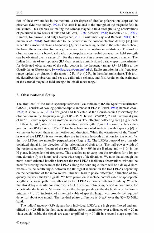
As a final step in the calibration of GRASP, we carried out observations towards the di-rection of the Galactic Center (GC) during the period March – July 2012. We specificallychose this period since the Sun was away from the Galactic Plane. Data were recorded inboth the LCP and RCP channels for ± four hours around the transit time (≈17:42 LocalSidereal Time: LST) of the GC across the local meridian at Gauribidanur. We assumed theradio emission from the direction of the GC to be randomly polarized in our case since cir-cularly polarized emission, if present, may be below the sensitivity limit of GRASP (Weilerand De Pater, 1983; Bowers, Falcke, and Backer, 1999), and it is difficult to observe lin-early polarized emission with the GRASP because of propagation effects (see Section 2).We therefore expect the average signal amplitude in the LCP and RCP channels over thefrequency range 85 – 35 MHz to be nearly equal. Any difference is most likely due to in-strumental and other errors (Figure 4). We would like to remark here that this is a noveland efficient scheme to calibrate the solar radio spectropolarimeter data, particularly at lowfrequencies, since radio emission from the direction of the GC is nonthermal in nature andhence intense at low frequencies. Once the offset between the LCP and RCP channels atdifferent frequencies are calibrated, the degree of circular polarization [dcp = V/I ] of theincident radiation can be estimated using the relation (ARCP −ALCP)/(ARCP +ALCP), whereA is the signal amplitude (see Section 2).

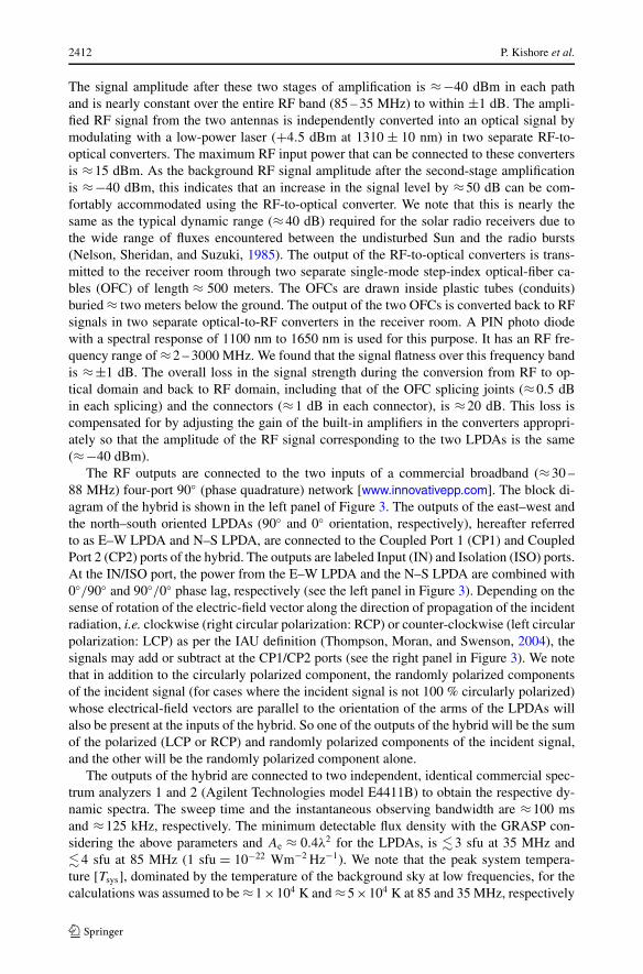
Figure 5 shows the results of the calibration scheme as applied to the GC observationswith the GRASP at a typical frequency of 65 MHz on 18 June 2014. The peak deflection inthe LCP and RCP channels (top panel) corresponds to the transit of the GC over the localmeridian in Gauribidanur. The dcp of the observed emission at 65 MHz is shown in the lowerpanel. It remains constant at zero (as expected) over an ≈ eight-hour period, indicating therobustness of the calibration. The variation in the dcp due to noise fluctuations is ≈±0.01.This indicates that GRASP can detect circularly polarized flux density to a minimum of

Gauribidanur Radio Spectropolarimeter 2415

Figure 4 Offset between the LCP and RCP channels of GRASP at different frequencies, as estimated fromthe observations in the direction of the Galactic Center.

Figure 5 Observations in the direction of the Galactic Center with the GRASP at a typical frequency of65 MHz. Top-left panel: LCP channel. Top-right panel: RCP channel. Lower panel: degree of circular polar-ization [dcp].

1 % of the total flux density. Routine observations in the direction of the GC indicate thatthe system is reasonably stable. We note that the offset errors in Figure 4 obtained fromobservations toward the direction of the GC are expected to be the maximum since thedeclination of the GC (≈−30◦ S) is almost at the half-power limit for the LPDAs used inthe GRASP (see Section 2). The latitude of Gauribidanur is ≈14◦ N. So the zenith angle ofthe GC for GRASP is ≈−44◦. This is smaller than the range of zenith angles (−37◦ to +9◦)for the Sun in a year, as seen from Gauribidanur.

4. Observations

Figure 6 shows the Stokes-I and Stokes-V dynamic spectra obtained from GRASP obser-vations on 4 February 2013 during the interval 08:07:00 – 08:11:00 UT. There are patches

2416 P. Kishore et al.

Figure 6 Stokes-I (upper panel) and Stokes-V (lower panel) dynamic spectra of a group of faint Type-IIIsolar radio bursts observed with the GRASP on 4 February 2013.

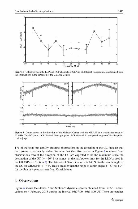
of intense emission drifting rapidly in frequency as a function of time in both spectra. Theseare the characteristic signatures of Type-III solar radio bursts from the solar corona (Suzukiand Dulk, 1985). The source region of the bursts was identified using the radioheliogramobtained with the Gauribidanur RAdioheliograPH (GRAPH: Ramesh et al., 1998; Ramesh,Subramanian, and Sastry, 1999; Ramesh, Sundara Rajan, and Sastry, 2006; Ramesh, 2011)at 80 MHz around the same time (Figure 7). The discrete source close to the eastern limb ofthe Sun corresponds to the Type-III burst at 80 MHz. Its average brightness temperature [Tb]is ≈108 K. This is about three orders of magnitude lower than the peak Tb of the Type-IIIradio bursts at 80 MHz (Suzuki and Dulk, 1985). An inspection of the soft-X ray emissionfrom the whole Sun obtained with the Geostationary Operational Environmental Satellite(GOES-15) on 4 February 2013 indicates that the X-ray activity at the time of the radiobursts mentioned above was at a low level [www.lmsal.com/solarsoft/latest_events/]. Thecorresponding energy in the 1 – 8 Å wavelength range was ≈2 × 10−7 Wm−2 (B2.0 class).No Hα flares were reported [www.swpc.noaa.gov/]. This indicates that the radio bursts inFigure 6 are probably associated with weak energy releases in the solar atmosphere (Kunduet al., 1986; Gopalswamy, Kundu, and Szabo, 1987; White, Kundu, and Szabo, 1987; The-jappa, Gopalswamy, and Kundu, 1990; Bastian, 1991; Subramanian, Gopalswamy, and Sas-try, 1993; Ramesh and Ebenezer, 2001; Ramesh et al., 2010, 2013). The close spatial cor-respondence between the source region of the Type-III bursts in Figure 7 and the sunspotActive Region AR 11669 (N05E79) observed on that day (i.e. 4 February 2013) indicatesthat the bursts might be associated with the latter. The above heliographic coordinates corre-spond to a viewing angle [θ ], i.e. the angle between the line of sight and the magnetic-field

Gauribidanur Radio Spectropolarimeter 2417

Figure 7 GRAPHradioheliogram obtained on4 February 2013 around08:09 UT at 80 MHz. Thediscrete source near the easternlimb is the location of theType-III bursts shown inFigure 6. Its peak Tb is ≈108 K.The contour interval is≈0.15 × 108 K. The open circleat the center represents the solarlimb. The size of the GRAPHbeam at 80 MHz is shown nearthe lower right corner.

Table 1 Details of the Type-III radio bursts.

Date Bursttime[UT]

Sunspotregionlocation

Viewingangle[θ]

X-rayflareenergy[Wm−2]

dcp85/35 MHz

B

85/35 MHz[G]

1 2 3 4 5 6 7

11 Nov 2012 05:55 N15E89 89◦ 6 × 10−7 0.16/0.04 8.0/0.8

17 Nov 2012 07:52 S28W88 88◦ 4 × 10−7 0.06/0.02 3.0/0.4

3 Dec 2012 04:35 N11E89 89◦ 2 × 10−7 0.06/0.05 3.0/1.0

7 Dec 2012 05:14 N15W89 89◦ 1 × 10−7 0.10/0.04 5.1/0.8

17 Dec 2012 05:34 N15W81 81◦ 4 × 10−7 0.22/0.07 11.1/1.5

4 Feb 2013 08:09 N05E79 79◦ 2 × 10−7 0.18/0.07 9.2/1.5

direction, of ≈89◦. The details related to this Type-III radio burst and the other similarevents reported in the present work are listed in columns 2 – 5 of Table 1.

5. Analysis and Results

Wild, Sheridan, and Nylan (1959) pointed out that both the fundamental [F] and the har-monic [H] Type-III solar radio burst emission should generally only be observable for eventsnear the center of the solar disk. It should be purely H-emission elsewhere. This is becausethe F-emission is more directive than the H-emission. According to Caroubalos and Stein-berg (1974), ground-based observations of Type-III radio bursts associated with sunspotregions located �70◦ either to the East or West of the central meridian on the Sun are pri-

2418 P. Kishore et al.

marily H-emission. Suzuki and Sheridan (1982) found that the F-component has a limitingdirectivity of ±65◦ from the central meridian on the Sun. A similar result was recentlyreported by Thejappa, MacDowall, and Bergamo (2012) for the very low frequency solarType-III radio bursts observed in the interplanetary medium. This is most likely due to thelarger free–free optical thickness of the overlying layer for the fundamental emission ascompared to the second-harmonic emission at the same frequency.

The heliographic longitude of the sunspot regions associated with the Type-III radiobursts in the present case are all �80◦ (column 3 in Table 1). The estimated dcp, partic-ularly at 85 MHz and 35 MHz (the highest and lowest observing frequency, respectively,in the present case), for all of the events in the present work (column 6 in Table 1) indi-cates that they are consistent with the average dcp (≈0.11) and the range of dcp (≈0 – 0.3)reported for the circularly polarized H-component of the Type-III bursts in the O-mode(Suzuki and Sheridan, 1978; Dulk and Suzuki, 1980a). These arguments indicate that theType-III bursts in the present case are probably due to H-emission. The sense of polar-ization was assumed to be the O-mode for of the following reasons: i) the Type-III radiobursts are due to plasma emission, and their polarization is predominantly in the O-modefor the F- and H-components (Melrose, Dulk, and Gary, 1980); ii) the X-mode emission ex-periences greater absorption than the O-mode during propagation through the solar corona(Fomichev and Chertok, 1968; Thejappa, Zlobec, and MacDowall, 2003).

Melrose, Dulk, and Smerd (1978), Melrose, Dulk, and Gary (1980), Zlotnik (1981), andWilles and Melrose (1997) have shown that when the Langmuir waves are collimated in thedirection of the magnetic field, weakly polarized H-radiation results with the sense of theO-mode, and the magnetic-field strength [B] near the source region of a solar radio burst(H-component) is related to the observed dcp as

B = fpdcp

2.8a(θ, θ0), (1)

where fp is the plasma frequency of the H-component in MHz and B is the magnetic-fieldstrength in Gauss. We assumed fp = f/2, where f is the frequency of observation, since theobserved emission in the 85 – 35 MHz band is most likely the H-component (see previousparagraph). a(θ, θ0) is a slowly varying function that depends on the viewing angle θ and theangular distribution θ0 of the Langmuir waves. In the present case, θ ≈ 79◦ – 89◦ (see col-umn 4 in Table 1). But each event can have a range of θ -values since the field lines emergingfrom the associated active region can diverge and/or expand nonradially (Dulk, Melrose, andSuzuki, 1979; Klein et al., 2008; Morosan et al., 2014). Reports indicate that the sizes of theType-III bursts fill a cone of angle θ ≈ 50◦ – 90◦, particularly when the source region is nearthe limb, as in the present case (Dulk, Melrose, and Suzuki, 1979; Dulk and Suzuki, 1980b).Similarly, the Langmuir wave vectors can be present in a cone of angle θ0 ≈ 30◦ with re-spect to the local magnetic-field direction for harmonic Type-III emission in the O-mode(Melrose, Dulk, and Smerd, 1978; Melrose, Dulk, and Gary, 1980; Zlotnik, 1981; Dulkand Suzuki, 1980a; Willes and Melrose, 1997; Benz, 2002). Taking into consideration thispossible spread in the θ and θ0 values, we find that a(θ, θ0) ≈ 0.2 – 0.4 in the present case(Suzuki and Dulk, 1985). Assuming the average value, i.e. a(θ, θ0) ≈ 0.3, we estimated themagnetic-field strengths for the different Type-III events listed in Table 1. The correspond-ing values, particularly at 85 MHz and 35 MHz, are listed in column 7 of Table 1. Theminimum and maximum B vary by a factor of ≈ four. An inspection of column 6 in Table 1indicates that this variation comes from the spread in the dcp values, which in turn might bedue to differences in the sizes of the corresponding bursts. Note that smaller sources near the

Gauribidanur Radio Spectropolarimeter 2419

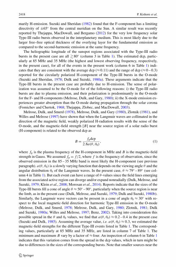
Figure 8 Variation of the estimated magnetic-field strength [B] with radial distance in the solar atmospherefor the Type-III bursts listed in Table 1. The vertical lines represent the range of B values at a particularfrequency/radial distance estimated from the different Type-III bursts listed in Table 1. The dashed line is thepower-law fit to the mean B (indicated by the circles) at each r .

limb can have higher dcp than larger sources (Dulk, Melrose, and Suzuki, 1979). In thesecases, accurate information on the source sizes is necessary since a smaller source near thelimb can also have a comparatively higher value for a(θ, θ0) (Suzuki and Dulk, 1985). Thisimplies that B will not vary linearly with dcp as in the present case (see Equation (1)).Unfortunately, the angular resolution in the present study is limited (≈5′ × 7′). However,considering the fact that the field strengths in Table 1 correspond to different solar activeregions, they can be regarded as reasonable (Dulk and McLean, 1978; Gopalswamy et al.,1986; Mercier, 1990; Fineschi, van Ballegoijen, and Kohl, 1999; Lin, Kuhn, and Coulter,2004; Lin, Penn, and Tomczyk, 2000; Vršnak et al., 2002; Mancuso et al., 2003; Rameshet al., 2005; Tomczyk et al., 2008; Ramesh, Kathiravan, and Sastry, 2010; Zucca et al.,2014). Figure 8 shows the variation of B over r ≈ 1.3 – 2.0 R� for all the Type-III burstsreported in the present work assuming the hybrid model of Vršnak, Magdalenic, and Zlobec(2004) for the electron-density distribution in the solar corona. We note that since the softX-ray flare energies corresponding to all the Type-III bursts in the present work are nearlythe same (column 5 of Table 1), we may be justified in using the same density model for allthe events. The power-law fit to the data points with 95 % confidence bounds (dashed linein Figure 8) indicates that B = 0.1(r − 1)−3.5 in the distance range 1.3 � r � 2.0 R�.

6. Summary

We have reported on the recently commissioned low-frequency (85 – 35 MHz) radio spec-tropolarimeter for dedicated observations of the solar corona at the Gauribidanur Obser-vatory, on the novel scheme to calibrate the observed circularly polarized radio emission,and on first results on the estimates of the coronal magnetic field [B] using observationsof Type-III radio bursts associated with sunspot regions close to the solar limb with thisinstrument. We only selected events with dcp � 0.2 whose associated source region wasclose to the limb of the Sun. These were the criteria to identify a harmonic Type-III burst.We also limited ourselves to data obtained close to the transit of the Sun across the localmeridian at Gauribidanur to minimize possible errors in the observed burst position dueto propagation effects (Stewart and McLean, 1982; Mercier, 1996,Ann). Our estimates in-dicate that B ≈ 0.1(r − 1)−3.5 over r ≈ 1.3 – 2.0 R�. This empirical relation is similar tothat reported earlier from spectral observations of Type-II radio bursts (Vršnak et al., 2002;

2420 P. Kishore et al.

Mancuso et al., 2003), Type-I radio bursts (Gopalswamy et al., 1986), and the combinationof different types of solar radio bursts (Dulk and McLean, 1978). The difference is that ourestimates were derived using direct observations of the associated circularly polarized radioemission. We note that more than 90 % of the Type-III radio bursts occur in the absenceof flares, and some 70 % of X-ray flares occur without Type-III radio bursts (Dulk, 1985).Therefore contemporaneous imaging and spectropolarimeter observations of low-frequencysolar radio bursts, particularly over the range 1.2 R� � r � 2 R� where simultaneous ob-servations of the corona against the solar disk as well as off the solar limb are rare as yet,can be a useful tool for inferring the coronal magnetic field associated with particularly theweak-energy releases in the solar atmosphere, since the related nonthermal radio emissioncan be easily detected (Benz and Kruger, 1995; Li, Cairns, and Robinson, 2009).

Acknowledgements We thank the staff of the Gauribidanur Observatory for their help in observations andthe maintenance of the antenna/receiver systems there. Ch.V. Sastry and C. Monstein are thanked for dis-cussions about circular polarization observations using phase-quadrature hybrids. We also thank the referee,whose comments helped us to present our results more clearly. We acknowledge the National GeophysicalData Center (NGDC) for providing open access to GOES data.

We have no conflict of interest concerning the work presented here.

References

Bastian, T.S.: 1991, Astrophys. J. Lett. 307, L49.Benz, A.O.: 2002, Plasma Astrophysics: Kinetic Processes in: Solar and Stellar Coronae, Astrophys. Space

Sci. Lib. Kluwer Academic, Dordrecht, 279.Benz, A.O., Kruger, A. (eds.): 1995, Coronal Magnetic Energy Releases, Lecture Notes in Physics 444,

Springer, Berlin, 1.Benz, A.O., Monstein, C., Meyer, H., Manoharan, P.K., Ramesh, R., Altyntsev, A., et al.: 2009, Earth Moon

Planets 104, 277.Bowers, G.C., Falcke, H., Backer, D.C.: 1999, Astrophys. J. Lett. 523, L29.Caroubalos, C., Steinberg, J.-L.: 1974, In: Newkirk, G.A. (ed.) Coronal Disturbances, IAU Symp. 57, Reidel,

Dordrecht, 239.Carrel, R.: 1961, IRE International Convention Record 9, 61.Dulk, G.A.: 1985, Annu. Rev. Astron. Astrophys. 23, 169.Dulk, G.A., McLean, D.J.: 1978, Solar Phys. 57, 279. ADS. DOI.Dulk, G.A., Melrose, D.B., Suzuki, S.: 1979, Publ. Astron. Soc. Aust. 3, 375.Dulk, G.A., Suzuki, S.: 1980a, Astron. Astrophys. 88, 203.Dulk, G.A., Suzuki, S.: 1980b, Astron. Astrophys. 88, 218.Ebenezer, E., Subramanian, K.R., Ramesh, R., Sundara Rajan, M.S., Kathiravan, C.: 2007, Bull. Astron. Soc.

India 35, 111.Fineschi, S., van Ballegoijen, A., Kohl, J.L.: 1999, In: Vial, J.-C., Kaldeich-Schümann, B. (eds.) Plasma

Diagnostics in the Solar Transition Region and Corona, Proc. 8th SOHO Workshop SP-446, ESA, No-ordwijk, 317.

Fomichev, V.V., Chertok, I.M.: 1968, Soviet Astron. 12, 21.Gelfreikh, G.B.: 2004, In: Gary, D.E., Keller, C.U. (eds.) Solar and Space and Future Development, Astro-

phys. Space Sci. Lib. 314, Kluwer Academic, Dordrecht, 115.Gopalswamy, N., Kundu, M.R., Szabo, A.: 1987, Solar Phys. 108, 333. ADS. DOI.Gopalswamy, N., Thejappa, G., Sastry, Ch.V., Tlaimcha, N.: 1986, Bull. Astron. Inst. Czechoslov. 37, 115.Grognard, R.J.M., McLean, D.J.: 1973, Solar Phys. 29, 149. ADS. DOI.Hariharan, K., Ramesh, R., Kishore, P., Kathiravan, C., Gopalswamy, N.: 2014, Astrophys. J. 795, 14.Iwai, K., Shibasaki, K.: 2013, Publ. Astron. Soc. Japan 65, S14.Kishore, P., Kathiravan, C., Ramesh, R., Barve, I.V., Rajalingam, M.: 2014, Solar Phys. 289, 3995. ADS.

DOI.Klein, K.-L., Krucker, S., Lointier, G., Kerdraon, A.: 2008, Astron. Astrophys. 486, 589.

Gauribidanur Radio Spectropolarimeter 2421

Kuhn, J.R., Penn, M.J. (eds.): 1995, Infrared Tools for Solar Astrophysics: What’s Next? World Scientific,Singapore, 89.

Kundu, M.R., Gergely, T.E., Szabo, A., Loiacono, R., White, S.M.: 1986, Astrophys. J. 308, 436.Li, B., Cairns, I.H., Robinson, P.A.: 2009, J. Geophys. Res. 114, A02104.Lin, H., Kuhn, J.R., Coulter, R.: 2004, Astrophys. J. Lett. 613, L177.Lin, H., Penn, M.J., Tomczyk, S.: 2000, Astrophys. J. Lett. 541, L83.Mancuso, S., Raymond, J.C., Kohl, J., Ko, Y.-K., Uzzo, M., Wu, R.: 2003, Astron. Astrophys. 400, 347.McLean, D.J.: 1985, In: McLean, D.J., Labrum, N.R. (eds.) Solar Radiophysics, Cambridge University Press,

Cambridge, 37.Melrose, D.B., Dulk, G.A., Gary, D.E.: 1980, Publ. Astron. Soc. Aust. 4, 50.Melrose, D.B., Dulk, G.A., Smerd, S.F.: 1978, Astron. Astrophys. 66, 315.Melrose, D.B., Sy, W.N.: 1972, Aust. J. Phys. 25, 387.Mercier, C.: 1990, Solar Phys. 130, 119. ADS. DOI.Mercier, C.: 1996, Ann. Geophys. 14, 42.Morosan, D.E., Gallagher, P.T., Zucca, P., Fallows, R., Carley, E.P., et al.: 2014, Astron. Astrophys. 568, A67.Morris, D., Radhakrishnan, V., Seielstad, G.A.: 1964, Astrophys. J. 139, 551.Nelson, G.J., Sheridan, K.V., Suzuki, S.: 1985, In: McLean, D.J., Labrum, N.R. (eds.) Solar Radiophysics,

Cambridge University Press, Cambridge, 113.Pätzold, M., Bird, M.K., Volland, H., Levy, G.S., Seidel, B.L., Stelzried, C.T.: 1987, Solar Phys. 109, 91.

ADS. DOI.Ramesh, R.: 2011, In: Choudhuri, A.R., Banerjee, D. (eds.) Proc. Astron. Soc. India Conf., Sec. 2, 1st Asia-

Pacific Solar Physics Meeting, ASI, Banglore, 55.Ramesh, R., Ebenezer, E.: 2001, Astrophys. J. Lett. 558, L141.Ramesh, R., Kathiravan, C., Sastry, Ch.V.: 2010, Astrophys. J. 711, 1029.Ramesh, R., Kathiravan, C., Satya Narayanan, A.: 2011, Astrophys. J. 734, 39.Ramesh, R., Subramanian, K.R., Sastry, Ch.V.: 1999, Astron. Astrophys. Suppl. 139, 179.Ramesh, R., Sundara Rajan, M.S., Sastry, Ch.V.: 2006, Exp. Astron. 21, 31.Ramesh, R., Subramanian, K.R., Sundara Rajan, M.S., Sastry, Ch.V.: 1998, Solar Phys. 181, 439. ADS. DOI.Ramesh, R., Kathiravan, C., Satya Narayanan, A., Ebenezer, E.: 2003, Astron. Astrophys. 400, 753.Ramesh, R., Satya Narayanan, A., Kathiravan, C., Sastry, Ch.V., Udaya Shankar, N.: 2005, Astron. Astrophys.

431, 353.Ramesh, R., Kathiravan, C., Sundara Rajan, M.S., Barve, I.V., Sastry, Ch.V.: 2008, Solar Phys. 253, 319.

ADS. DOI.Ramesh, R., Kathiravan, C., Barve, I.V., Beeharry, G.K., Rajasekara, G.N.: 2010, Astrophys. J. Lett. 719,

L41.Ramesh, R., Sasikumar Raja, K., Kathiravan, C., Satya Narayanan, A.: 2013, Astrophys. J. 762, 89.Sasikumar Raja, K., Ramesh, R.: 2013, Astrophys. J. 775, 38.Sasikumar Raja, K., Kathiravan, C., Ramesh, R., Rajalingam, M., Barve, I.V.: 2013, Astrophys. J. Suppl. 207,

2.Schatten, K.H., Wilcox, J.M., Norman, F.: 1969, Solar Phys. 6, 442. ADS. DOI.Schrijver, C.J., Derosa, M.L.: 2003, Solar Phys. 212, 165. ADS. DOI.Spangler, S.R.: 2005, Space Sci. Rev. 121, 189.Stewart, R.T., McLean, D.J.: 1982, Publ. Astron. Soc. Aust. 4, 386.Subramanian, K.R., Gopalswamy, N., Sastry, Ch.V.: 1993, Solar Phys. 143, 301. ADS. DOI.Suzuki, S.: 1974, Solar Phys. 38, 3. ADS. DOI.Suzuki, S., Dulk, G.A.: 1985 In: Solar Radiophysics, Cambridge University Press, Cambridge, 289.Suzuki, S., Sheridan, K.V.: 1978, Quantum Electron. 20, 989.Suzuki, S., Sheridan, K.V.: 1982, Publ. Astron. Soc. Aust. 4, 382.Thejappa, G., Gopalswamy, N., Kundu, M.R.: 1990, Solar Phys. 127, 165. ADS. DOI.Thejappa, G., MacDowall, R.J., Bergamo, M.: 2012, Astrophys. J. 745, 187.Thejappa, G., Zlobec, P., MacDowall, R.J.: 2003, Astrophys. J. 529, 1234.Thompson, A.R., Moran, J.M., Swenson, G.W.: 2004, Interferometry and Synthesis in Radio Astronomy,

VCH, Weinheim, 100.Tomczyk, S., Card, G.L., Darnell, T., Elmore, D.F., Lull, R., Nelson, P.G., et al.: 2008, Solar Phys. 247, 411.

ADS. DOI.Vršnak, B., Magdalenic, J., Zlobec, P.: 2004, Astron. Astrophys. 413, 753.Vršnak, B., Magdalenic, J., Aurass, H., Mann, G.: 2002, Astron. Astrophys. 396, 673.Weiler, K.W., De Pater, I.: 1983, Astrophys. J. Suppl. 52, 293.Weiler, K.W., Raimond, E.: 1976, Astron. Astrophys. 52, 397.White, S.M.: 2005, In: Innes, D.E., Lagg, A., Solanki, S.K. (eds.) Chromospheric and Coronal Magnetic

Fields, SP-596, ESA, Noordwijk, 10.

2422 P. Kishore et al.

White, S.M., Kundu, M.R., Szabo, A.: 1987, Solar Phys. 107, 135. ADS. DOI.Wild, J.P., Sheridan, K.V., Nylan, A.A.: 1959, Aust. J. Phys. 12, 369.Willes, A.J., Melrose, D.B.: 1997, Solar Phys. 171, 393. ADS. DOI.Zlotnik, Ia.E.: 1981, Astron. Astrophys. 101, 250.Zucca, P., Carley, E.P., Bloomfield, D.S., Gallagher, P.T.: 2014, Astron. Astrophys. 564, A47.