A Kinked-Demand Theory of Price Rigidity

Stéphane Dupraz∗

Columbia University

November 12, 2016

(JOB MARKET PAPER)

Abstract

I provide a microfounded theory for one of the oldest, but so far informal, explanations of price

rigidity: the kinked demand curve theory. Assuming that some customers observe at no cost only the

price of the store they happen to be at gives rise to a kink in firms’ demand curves: a price increase

above the market price repels more customers than a price decrease attracts. The kink in turn makes a

range of prices consistent with equilibrium, but an intuitive criterion—the adaptive rational-expectations

criterion—selects a unique equilibrium where prices stay constant for a long time. The kinked-demand

theory is consistent with price-setters’ account of price-rigidity as arising from the customer’s—not the

firm’s—side, and can be tested against menu-cost models in micro data: it predicts that prices should be

more likely to change if they have recently changed, and that prices should be more flexible in markets

where customers can more easily compare prices. The kinked-demand theory has novel implications

for monetary policy: its Phillips curve is strongly convex but does not contain any (present or past)

expectations of inflation; its trade-off between output and inflation persists in the long-run; changes

to the distribution of sectoral productivity shift the Phillips curve; and monetary shocks have a much

longer-lasting real effect than in a menu-cost model, despite also being a model of state-dependent pricing.

∗Email: stephane.dupraz@columbia.edu. I am indebted to my advisors Ricardo Reis and Michael Woodford for their

continuous guidance and support. I also greatly benefited from discussions and comments from Keshav Dogra, Andres Drenik,

Kate Ho, Navin Kartik, Jennifer La’O, Filip Matejka, Emi Nakamura, Bernard Salanié, and Jón Steinsson.

1

Introduction

Why are prices sticky? Most monetary macro models—when they do not assume that firms cannot change

their prices for a number of periods—have looked for a rationale for nominal rigidities on the firm’s side.

Menu-cost models assume that a firm can calculate its desired price for free, but adjusts its posted price to

its desired level at a cost.1 Models of producers’ inattentiveness assume that a firm can adjust its posted

price for free, but uncovers its desired price at a cost.2 Both classes of models face a theoretical difficulty:

if prices do not adjust, quantities must. Menu-cost models need to assume that quantity adjustment-costs

(hiring costs) are less important than price adjustment-costs, while models of producers’ inattentiveness need

to assume that firms do not notice that they produce and hire more.

But firm-side models of price rigidity also face an empirical challenge: surveys of price-setters repeatedly

point instead at the customer’s side as the source of price rigidity.3 When asked “why they don’t change their

prices more often than that”, a majority of price-setters surveyed by Blinder et al. (1998) stress their fear of

“antagonizing customers”. The answer is vague.4 But price-setters seem to be telling us they charge a fixed

price not because their desired price is too costly to implement or too difficult to learn about, but because

their desired price itself is sticky. They point at customers’ reaction to price changes: demand curves.

A persistent, if less prominent, literature in monetary economics has sought a rationale for price rigidity

on the customer’s side, appealing to ideas of implicit contracts and fairness, customer-base markets, or

customers’ search. A likely reason for their lesser popularity, customer-side arguments for price rigidity

often lack the microfoundations of their firm-side counterparts. As a result, their internal consistency, and

the key assumptions that distinguish them from the benchmark models of consumer demand, have remained

open questions. This is in particular true of one of the oldest, and at a time leading, theories of price rigidity:

the kinked demand curve theory, dating back to Hall and Hitch (1939) and Sweezy (1939).5

I provide microfoundations—optimizing behaviors, standard equilibrium concepts and rational expectations—

for the old informal argument for price rigidity of the kinked-demand curve. I show that relaxing a single

assumption on customers in a model of imperfect competition gives rise to a kink in firms’ demands: that

all customers are equally informed on all prices charged by firms within a market. When instead some

customers observe at no cost only the price at the firm they happen to be at, firms’ demands become kinked:1Menu-cost models include Caplin and Spulber (1987); Caballero and Engel (1991, 1993) for a monotonic increase in nominal

spending and one-sided (S,s)-policies, and Caplin and Leahy (1991, 1997) for a symmetric nominal spending process and two-sided (S,s)-policies. Danziger (1999); Dotsey et al. (1999); Danziger and King (2005); Golosov and Lucas (2007); Nakamuraand Steinsson (2010); Midrigan (2011) consider operational DSGE versions of the menu-cost model.

2The renewed interest in models of producers’ inattentiveness was kindled by Mankiw and Reis (2002)’s model of delayedinformation and Woodford (2003a)’s model of partial information. The subsequent literature has endogenized the informationstructure by modeling the information choice, as in Reis (2006); Woodford (2009); Mackowiak and Wiederholt (2009). Alvarezet al. (2011) combine observation and menu costs.

3See Blinder (1991) and Blinder et al. (1998) for the United-States, Fabiani et al. (2007) for the eurozone, Hall et al. (1997)and Greenslade and Parker (2012) for the United Kingdom, Amirault et al. (2004) for Canada, and Apel et al. (2005) forSweden.

4One could interpret price-setters’ answer as simply referring to the price-elasticity of demand: when prices increase, cus-tomers are antagonized, so they leave and demand falls. This is the puzzle: standard models of either perfect or imperfectcompetition very much incorporate elastic demand curves. Yet they predict prices should be flexible.

5On the history of the kinked-demand curve theory, see Reid (1981) and Stigler (1978).

2

a firm loses more customers by increasing its price above the market price than it gains by decreasing it

below. The kink in demand in turn justifies prices that stay constant for substantial periods of time, despite

firms’ ability to change them at any moment and at not cost. Although imperfect competition alone does

not account for price rigidity, it does when coupled with customers’ asymmetric information on prices. It

does so though firms have perfect information on all shocks, though no agent is subject to money illusion,

and in tune with price-setters’ reported impression that keeping prices fixed is their optimal response even

in the absence of any physical or cognitive constraint on changing prices.

To isolate the key assumption responsible for flexible or sticky prices, I proceed by step-by-step departures

from the benchmark model of price-setting under imperfect competition: monopolistic competition in face

of the consumption aggregator of a representative agent.6 There, demand is elastic at the intensive margin

only—when prices increase, customers can buy fewer goods. My first departure is to consider instead a

switching-cost model where demand is also elastic at the extensive margin—when prices increase, customers

can leave to competitors (section 2). I introduce the extensive margin of demand in a way that preserves

the tractability of the benchmark model: the only difference is that the elasticity of demand is now the sum

of the elasticities at the intensive and extensive margins. The introduction of the extensive margin in itself

does not make prices sticky: I show that when customers (and firms) have perfect information, prices are

flexible and the classical dichotomy holds.

Yet, the new framework allows me to consider alternative assumptions on the information available to

customers. I relax the assumption that all customers know all prices in a market. Instead, I assume that a

fraction of them observe at no cost only the price at the firm they happen to be at, and need to first move to

a competitor to observe its price (section 3). Customers are not subject to money illusion however: they all

have perfect information on the distribution of prices in all markets, and therefore on the price level. This

single assumption gives rise to a kink in a firm’s demand curve, located at the market price: all customers at

the firm notice and react to a price increase, but only a fraction of customers at other firms notice and react

to a price decrease. This provides microfoundations for the informal theory of the kinked-demand curve first

propounded by Sweezy (1939) and Hall and Hitch (1939), especially the versions of the argument relating

the existence of the kink to information asymmetries (Scitovsky (1978); Stiglitz (1979); Woglom (1982)).7

As conjectured by Woglom (1982) however, the implication of the kink is not price rigidity. Instead, it is

price-multiplicity: a whole range of equilibrium prices are possible in a given market, and the indeterminacy

translates into an indeterminacy at the macro level. The possible equilibrium prices are all higher or equal

to the full-information price. The competitive force that drives prices down under full-information—the

incentive to attract new customers with lower prices—is no longer effective.

The multiplicity is a fragile theoretical feature however. The root of multiplicity is the same as in menu-

cost models: strategic complementarities. If all storekeepers wake up one morning expecting everyone else6This benchmark is spelled out for instance in section 1.1 of chapter 3 of Woodford (2003b).7In Hall and Hitch (1939)’s and Sweezy (1939)’s initial formulation, the kink is argued to come instead from competitors’

(real or imagined) reactions to price changes: competitors are feared to react more to a price decrease than to a price increase.

3

to switch to a new price, then it is in every storekeeper’s interest to follow the herd. Such an extent of

coordination seems unrealistic. To capture the intuition that firms are reluctant to be the first firm to

raise prices in the market—a reluctance price-setters rank very high in surveys as the reason why they do

not change prices—I define a new equilibrium selection criterion: I assume price-setters start each period

using yesterday’s price as their initial guess for what the market price will be today, deduce all firms’ best

response to this price, and iterate until the guessed price is the best-response price. Firms’ mental process is

adaptive, but expectations are ultimately always rational: I call such equilibria adaptive rational-expectations

equilibria. I show that there exists a unique adaptive rational-expectations equilibrium. In it, a firm’s pricing

function features an inaction region: prices are sticky (section 4).

Menu-cost models too predict infrequent price changes. Does the kinked-demand theory make predictions

that distinguishes it from menu-cost models? I stress two micro-level predictions that set the theory apart

and make it testable (section 5). I restrict to predictions that are robust to the assumption on the process for

costs, so I venture away from statistics such as the frequency and size of price changes, which are the joint

product of a theory and a process for costs. First, the kinked-demand theory predicts that prices should be

more likely to change if they have recently changed: hazard functions should be decreasing at first. Second,

it predicts that prices should be more flexible in markets where customers can more easily compare prices.

I find evidence of both in the empirical literature.

Turning from the micro to the macro, I show that the kinked-demand theory has novel implications

for monetary policy (section 6). First, the Phillips curve of the kinked-demand theory is strongly convex

but does not contain any inflation expectations shifters. The strong convexity limits the extent to which

inflation can increase output despite the absence of expectation shifters. Yet the absence of expectations

shifters implies that disinflation remains costly even when the change in monetary policy is not only credible,

but also widely known. The convexity also explains the flattening of the Phillips cure since the early 1980s,

and the missing disinflation during the Great Recession. Second, the kinked-demand theory predicts a

long-run trade-off between output and inflation: the long-run Phillips curve is non-vertical. Third, in

the kinked-demand theory relative price changes such as oil price shocks shift the Phillips curve up, and

monetary policy can undo these inflationary pressures only at the cost of a decrease in output. Fourth, the

kinked-demand theory, despite being a model of state-dependent pricing, predicts long-lasting real effects of

monetary shocks, if anything even longer-lived than in a comparable Calvo model. It shows that the often

short-lived effects of monetary shocks found in menu-cost models are no feature of state-dependent pricing

per se: endogenizing the changing response of price-setting to a changing environment needs not write down

the extent of monetary non-neutrality

4

1 Literature review

This paper is not the first one to look for a rationale for price rigidity on the customer’s side. Several strands

of the literature have considered reasons why customers may behave differently than the canonical model

of demand predicts. Although these papers differ enough to be classified into different subliteratures, they

often start from the same desire to reconcile demand theory with the perception of practitioners. As such,

they can be seen as various attempts to rationalize a common idea. (Because many of these papers lack

microfoundations, whether they tell the exact same story is ultimately subjective.) Since the present paper

certainly belongs to the same effort, I contrast the different models with the present rationalization. If the

single assumption of customers’ asymmetric information is enough to give a theory of demand that makes

prices sticky, what assumptions are not necessary?

Several papers appeal to the ideas of fairness or implicit norms to justify price rigidity. Okun (1981)

suggests firms do not change their prices so often because they have “implicit contracts” with their customers

not to take advantage of them by raising prices when demand is high. Whether Okun’s contracts are meant

to be enforced by reputation concerns or constitute social norms is unclear. Other authors like Kahneman

et al. (1986) or Rotemberg (2005) make a more explicit appeal to the notion of fairness. I show that a

customer-side theory of price-rigidity needs not arise from concerns about fairness. I derive firms’ incentives

not to vary prices using standard preferences and equilibrium concepts.

Following Phelps and Winter (1970), customer-base models consider markets where firms and customers

interact repeatedly. If customers learn slowly about prices charged by different competitors, Phelps and

Winter conjecture, customers should flow only slowly from expensive to cheap stores. Current prices should

thus have little impact on demand today, but much on demand tomorrow, providing incentives for firms

not to adjust their prices to short-term variations in costs. A main challenge in modeling the intuition

behind customer-base markets is to keep track of the dynamics of market shares. Ravn et al. (2006) find an

ingenious way to circumvent the aggregation problem by keeping demand elastic at the intensive margin—

not the extensive margin—and basing firms’ market-share concerns on customers’ building habits in their

goods—not on the slow diffusion of information. Soderberg (2011) also dispenses with the extensive margin of

demand, but returns to an informational interpretation of a customer-base by having the representative agent

only occasionally reoptimizing its allocation of consumption. These microfounded models do not produce

sticky prices however. An exception is Nakamura and Steinsson (2011) who show in a customer-base model

based on habits formation that price rigidity is one (of many) possible equilibrium outcome because it allows

firms to commit not to price-gouge their customers. Their model may be seen as a rationalization of the

fairness argument.

The model of this paper shares with the customer-base literature the focus of its early papers on the ex-

tensive margin of demand and on customers’ imperfect information. In contrast however, I do not emphasize

the intertemporal considerations associated to a customer-base: although in the model a customer starts a

period attached to one firm and can switch to another only by incurring a cost, I assume the customer is

5

randomly reassigned to a new firm in the next period. Thus, although the model is a switching-cost model

(Klemperer (1987); Farrell and Klemperer (2007)), it may well not deserve the name of a customer-base

model.8 The abstraction from the dynamics of firms’ market-shares is intentional: it stresses that the ratio-

nale for price rigidity presented in this paper does not rely on firms’ forward-looking considerations on the

evolution of their customer-bases.

Another literature the paper connects to is the good-market search literature. The connection is different.

The kinked-demand papers of Stiglitz (1979) and Woglom (1982) appealed to customer search to postulate

a kink. Yet, the microfounded customer-search literature seldom addressed the question of price rigidity,

and focused instead on other issues, first of which the possibility of price dispersion in equilibrium.9 At

any rate, the microfounded papers show no kink in demand.10 This raises two questions. Is the present

kinked-demand model a search model? If so, how come it is the only one to find kinked demand curves?

Both questions are best answered through a concrete search model, so I take on them in a companion

paper, Dupraz (2016). Here, I jump to the bottom lines. On the first question: the present model is not

an explicit search model, but the kind of markets it seeks to capture can be seen as including markets

with search. The model shows that two departures from the benchmark theory of consumer demand are

enough to generate kinked demand curves: an extensive margin of demand, and asymmetrically informed

customers. Because a search model fulfills both requirements, the argument for a kink applies to a search

model. The companion paper shows this more concretely by re-deriving the argument of the present paper

within an explicit search model. So, to the second question: search models did not find a kink in demand

because most assumed search costs to be the same for all customers. When search costs are the same for all

customers, firms face discontinuous demand curves. If instead search costs are both continuously distributed

among customers and with a positive density at zero—as switching costs are in the framework of the present

paper—then demand curves are kinked. In other words, the kink in demand in search models has been

hidden by the discontinuity in demand arising from the particular assumption of homogeneous search costs.

Some papers have tackled the issue of providing microfoundations for the theory of the kinked-demand

curve. However, they microfound different arguments for the kink. Maskin and Tirole (1988) analyze the8Kleshchelski and Vincent (2009) argue that switching costs can bring the pass-through between costs and prices below one-

for-one. In contrast, in the model of this paper, switching costs alone do not account for price rigidity. Only with informationasymmetries—absent in their paper—do they generate sticky-prices, in the strong sense of no pass-through at all for extendedperiods of time.

9See McMillan and Rothschild (1994) for a survey of the search literature. A small branch of the search literature—the Bayesian search models of Benabou and Gertner (1993); Fishman (1996); Dana (1994)—does address monetary issues.However, the mechanism these models focus on does not go through a kink in demand: the Bayesian search literature considersthe inference that a customer can make from one firm’s price on the distribution of prices in the market. Benabou and Gertner(1993) study how inflation can increase customers’ search, and therefore competition in the market. Dana (1994) shows thatthe price level is less responsive to cost changes than under customers’ full information. Fishman (1996) shows that cost shockshave different short-term and long-run effects on prices. Independently of the Bayesian search literature, and still distinct fromthe kinked-demand curve, Head et al. (2012) make the case that in a search model with price dispersion, the unique equilibriumdistribution of prices can be implemented through several pricing policies by individual firms, some of which consist in keepingprices fixed for many periods.

10Stiglitz (1987) claims to prove the existence of a kink. However, as Stahl (1989) notes: “[Stiglitz] makes the dubiousassumption that consumers can "see" deviations by stores before they actually search. This departure from the notion of anNE is crucial to [his] results.” Whether the assumption is considered dubious or not, it rules out in any case the mechanismthat drives the kink in the present paper: that some customers do not notice firms’ price decreases. The same remark appliesto Braverman (1980) (who is not interested in price rigidity).

6

Markov-perfect equilibrium of a dynamic price-competition model where firms take turns choosing prices.

They show that some equilibria are reminiscent of the kinked-demand theory because a price decrease triggers

a price war while competitors do not react to a price increase. As such, Maskin and Tirole microfound Hall

and Hitch (1939)’s and Sweezy (1939)’s argument for a kink in demand. Besides, they do not address the

question of the responsiveness of prices to changing costs: costs do not fluctuate in their model. Heidhues

and Koszegi (2008) generate kinked demand curves by assuming that consumers are loss averse relative to

some expectation they have formed on the price. In a recent paper, Ilut et al. (2015) propose a theory of

price rigidity that arise through a kink in the perceived demand curve of firms: a combination of Knightian

uncertainty and non-parametric learning generates a kink in the expected demand of a firm as the firm

fears the worst if it changes its price. Yet demand is in reality smooth. In contrast, I show that demand is

effectively kinked when some customers are asymmetrically informed on prices. Firms perceive demand to

be kinked because it is.

Although the kinked-demand theory receded from monetary macroeconomics in the 1970’s, Kimball

(1995) reintroduced a modified version in the 1990’s: quasi-kinked demand curves. Quasi-kinked demand

curves—which Kimball postulates—capture the same general intuition as kinked-demand curves: firms lose

more customers by raising their prices above the market price than they gain by lowering them below. But

the kink of a quasi-kinked demand curve is smoothed-out. This matters: quasi-kinked demand curves do

not produce price rigidity. Instead, Kimball shows that they amplify existing sources of price rigidity by

increasing strategic complementarities. Levin and Yun (2008) consider a search model that produces quasi-

kinked demand curves. The model of this papers produces an unadulterated kink, and therefore a basis for

price rigidity.

Finally, other recent papers tackle the issue of price rigidity and consumers’ imperfect information through

different mechanisms. Matejka (2011) considers the information choice of rationally-inattentive costumers

and shows it can make fixed prices appealing to price-setters. The mechanism Matejka investigates relies

on customers’ aversion to variations in their consumption of the numeraire. L’Huillier (2015) considers a

monopolist facing consumers who are uninformed about the level of inflation. He shows that the monopolist

can benefit from charging a fixed price in order not to tip off customers about the inflation rate. Because

L’Huillier’s model (and Matejka’s) considers a monopoly, it does not address the mechanism that I stress:

the nature of competition when customers are unequally informed on all competitors’ prices.

2 The extensive margin of demand

In this section, I introduce a general-equilibrium set-up that distinguishes between the intensive and extensive

margins in a firm’s demand. I present the set-up absent any form of frictions—in particular all households

and all firms have perfect information—and show that price flexibility and monetary neutrality hold in this

case. This establishes the benchmark to which subsequent sections are compared.

7

The economy engages in the production of the continuum of goods i ∈ [0, 1] from an homogeneous labor

input, each consumed by a continuum of households j ∈ [0, 1]. Good i is produced in sector i, by any of a

continuum of firms k ∈ [0, 1]—each firm is designated by the double index i, k. Firms are price-setters; the

labor market is competitive. Although customers are perfectly indifferent between all goods sold in market

i once acquired, competition in market i is hindered by the existence of switching costs: each customer j is

initially attached to one firm, knows of one firm he can switch to at a cost, and cannot shop at any other

firm.

2.1 Households

All households j have the same intertemporal preferences over a continuum of goods i ∈ [0, 1] at each period,

and labor at each period:

E0

∞∑t=0

βt(log(Cjt )− Ljt ), (1)

where Ljt is hours worked and Cjt is total consumption defined as the CES aggregator of the consumption of

all goods i:

Cjt =(∫

i

(Cjt,i)θ−1θ di

) θθ−1

. (2)

Household j starts a period t with nominal wealth Bt and has access to complete financial markets, where

Qt,t+1 is the unique nominal stochastic discount factor. On each market i customer j is randomly assigned at

the beginning of each period t to one firm Aji , to which he has free access. (Every day, he goes shopping and

randomly bumps first into one shop.) In addition, customer j randomly draws a second firm Bji , to which

he can switch only by incurring a cost. (He notices another shop, a few blocks down the street.) Finally,

customer j has no access to other firms k on market i. His shopping decision on market i therefore reduces

to whether to stay at Aji , or switch to Bji . The switching cost is expressed as a fraction of total consumption,

and is proportional to the size of market di: it is γji diCjt , where the proportionality factor γji ≥ 0 is specific

to both the customer and the market.

Once he has decided where to shop on all markets, household j faces a standard consumption problem

taking as given prices (P jt,i)i, where on a given market i, P ji,t is either PBj

t,i or PAjt,i depending on his switching

decision. His flow budget constraint is then:

∫P jt,iC

jt,idi+ Et(Qt,t+1B

jt+1) = WtL

jt + Πt +Bjt = Ijt , (3)

where Wt is the nominal wage, Πt nominal profits coming from the ownership of firms—I assume the

ownership of all firms is equally divided between all households—and Ijt denotes total nominal incomes.

8

(I assume that switching costs, although expressed in consumption equivalents, are incurred in effort and

therefore do not show up in the budget constraint). In addition, a terminal constraint forbids household j

to enter Ponzi-schemes.

Solve household j’s problem backward. After deciding where to shop, j consumes and works (and invests,

but I won’t use the optimal portfolio decisions) to maximize utility. The consumption/leisure trade-off sets:

Cjt = Wt

P jt, (4)

and demand for the individual good i takes the form:

Cjt,i =(P jt,i

P jt

)−θCjt , (5)

where P jt is the subjective price index of customer j:

P jt =(∫

(P jt,i)1−θdi

) 11−θ

. (6)

2.2 Household’s shopping decisions

Consider now the shopping problem of household j in market i. Because he is randomly reassigned to two

new firms Ai and Bi next period, j faces only present-period benefits of switching from firm Ai to firm Bi.

If he shops at firm Ai, customer j gets indirect utility Cj(PAi )—total consumption when the price of good

i is PAi ; if he shops at firm Bi, he gets indirect utility (1 − γji di)Cj(PBi )—the fraction 1 − γji di of total

consumption when the price of good i is PBi . He therefore switches to firm Bi if and only if:

Cj(PAi )Cj(PBi )

< 1− γji di (7)

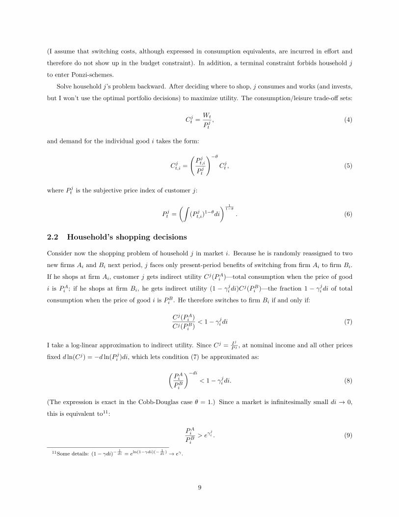
I take a log-linear approximation to indirect utility. Since Cj = Ij

P j , at nominal income and all other prices

fixed d ln(Cj) = −d ln(P ji )di, which lets condition (7) be approximated as:

(PAiPBi

)−di< 1− γji di. (8)

(The expression is exact in the Cobb-Douglas case θ = 1.) Since a market is infinitesimally small di → 0,

this is equivalent to11:

PAiPBi

> eγji . (9)

11Some details: (1− γdi)− 1di = eln(1−γdi)(− 1

di) → eγ .

9

In words: customer j switches to firm Bi when Ai’s price is more than (eγji − 1)% above Bi’s price.

2.3 Firm’s market share and firm’s demand

Look now at market i from firm k’s perspective. A fraction dk of customers have been randomly assigned

to firm k as their primary A-firm, and another fraction dk have been assigned to firm k as their secondary

B-firm. I consider symmetric equilibria in market i where all firms charge the same price Pi (so that there

will be ultimately no switching in equilibrium). If firm k charges the same price Pi as all other firms, it

maintains its initial market share dk. By charging a lower price, k can increase its market share up to 2dk

by attracting the customers who are not at k but can switch to it. In contrast, a higher price triggers the

departures of some of k’s own customers toward their secondary B-firm, and decreases k’s market share.

This exact way in which firm k’s market share responds to the price it charges is determined by the

distribution of switching costs γji ∈ R+ across customers, or equivalently the distribution of eγji ∈ [1,+∞). I

note F the CDF of the distribution of eγji (the same in all subgroups of customers defined by their primary

firm), and pk = P k/Pi the price of firm k relative to the market price. If k charges a higher price pk ≥ 1, then

k will retain only its customers with a large enough switching cost eγji ≥ pk: a fraction 1− F (pk). Besides,

k will attract no customer from other firms. Instead, if k charges a lower price pk, then k will retain all its

customers, and will attract those of other firms’ customers with switching costs small enough eγji ≤ 1/pk: a

fraction F (1/pk). The market share of firm k is therefore νdk, where ν is the market share function:12

ν(pk)≡

1− F (pk) if pk ≥ 1,

1 + F(1/pk

)if pk ≤ 1.

(10)

I assume F is a continuous and differentiable distribution. This guarantees that the market share function

ν is continuous and differentiable everywhere. In particular, it is differentiable at the relative price pk = 1,

which is where the elasticity of the market share function matters in a symmetric equilibrium. I note α

(minus) this elasticity:

α ≡ −εν(1) = F ′(1). (11)

As Klemperer (1987) notes, the elasticity of the market share is driven by the density of customers with no

switching costs: these are the marginal customers, who arbitrage any price discrepancy between firms.

The market-share function measures whether a customer buys or not at firm k: the extensive margin of

demand. On top of it, a customer who buys at k buys more or less depending on k’s price: the intensive

margin of demand. This last margin is the standard one incorporated in models of monopolistic competition12I call ν—and later s—the market share although it can be greater than one: it lies between 0 and 2. There is no contradiction:

what should be rigorously referred to as the market share is ν × dk < 1—and later on s × dk < 1. I proceed with the slightabuse of language.

10

pk0.5 0.6 0.7 0.8 0.9 1 1.1 1.2 1.3 1.4 1.50

0.2

0.4

0.6

0.8

1

1.2

1.4

1.6

1.8

2Fulll-information market share 8

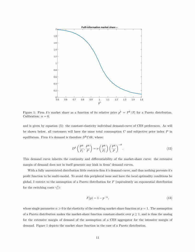
Figure 1: Firm k’s market share as a function of its relative price pk = P k/Pi for a Pareto distribution.Calibration: α = 6.

and is given by equation (5): the constant-elasticity individual demand-curve of CES preferences. As will

be shown below, all customers will have the same total consumption C and subjective price index P in

equilibrium. Firm k’s demand is therefore DkCdk, where:

Dk

(P k

Pi,P k

P

)= ν

(P k

Pi

)(P k

P

)−θ. (12)

This demand curve inherits the continuity and differentiability of the market-share curve: the extensive

margin of demand does not in itself generate any kink in firms’ demand curves.

With a fully unrestricted distribution little restricts firm k’s demand curve, and thus nothing prevents k’s

profit function to be multi-modal. To avoid this peripheral issue and have the local optimality conditions be

global, I restrict to the assumption of a Pareto distribution for F (equivalently an exponential distribution

for the switching costs γji ):

F (p) = 1− p−α, (13)

whose single parameter α > 0 is the elasticity of the resulting market-share function at p = 1. The assumption

of a Pareto distribution makes the market-share function constant-elastic over p ≥ 1, and is thus the analog

for the extensive margin of demand of the assumption of a CES aggregator for the intensive margin of

demand. Figure 1 depicts the market share function in the case of a Pareto distribution.

11

2.4 Firm’s pricing

Let us turn to firm k’s pricing decision. Firm k, as all other firms in sector i, uses the constant returns to

scale production function in labor Y = At,iL, where At,i is the state of technology in sector i at period t—I

allow for heterogeneity in technology across sectors, but assume homogeneity within sector i. Because firm

k gets to reset its price every period, and because customers are randomly reassigned every period so that

firm k’s price today does not affect its market share tomorrow, firm k sets its price P k to maximize present

profits πk = (P k − WAi

)Dk(P k)Cdk, taking the nominal wage W as given.

Because k’s demand curve (12) is differentiable, k’s optimal price needs to satisfy the first-order condition.

From this local optimality condition, the only possible symmetric equilibrium is thus for all firms to charge:

P k = Pi =M(α+ θ)WAi, (14)

whereM(ε) ≡ ε

ε− 1 is the Lerner markup function.

which is well-defined provided ε = θ + α > 1. The appendix checks that under the assumption of a Pareto

distribution, firms’ profit functions are single-peaked, and thus that this is indeed an equilibrium.

The market stays equally divided between all firms, and there is no switching in equilibrium. The markup

is determined by the total elasticity of demand ε = α+ θ, which is the sum of the elasticities of demand at

the intensive and extensive margins. The pricing decision is exactly identical to the pricing decision in the

representative-agent benchmark of consumer demand, except the elasticity is now the sum of the elasticities

at the intensive and extensive margins.13

2.5 Monetary neutrality

Because the pricing decision is the same as in the benchmark, monetary neutrality obtains as in the bench-

mark. Since on all markets all firms set the same price, all customers face the same prices on all markets

and there is no heterogeneity among households in equilibrium, as claimed earlier. The common subjective

price level (6) is given by:

P = M(α+ θ)WA

, (15)

where:

A ≡(∫

Aθ−1i dF (Ai)

) 1θ−1

, (16)

13The property of the benchmark of monopolistic competition and CES demand that prices are a constant markup over costsonly carries over here under the assumption that firms are homogeneous within a market. The symmetry between firms preventsthem to face the bottom part Pk < Pi of their demand curves (12) in equilibrium. I do not rely on this non constant-elasticcomponent of the demand curve here. Yet, when firms differ in their costs of productions, the model gives further insight intothe mechanisms of competition at the extensive margin: while higher-cost firms price a constant markup over their marginalcost, lower-cost firms set their price closer to the one of higher-cost firms.

12

where F is the cross-sectional distribution of productivity across markets, and A is a measure of aggregate

productivity. Equation (15) sets the real wage W/P to A/M(α+ θ). The real wage is in turn equal to the

marginal rate of substitution between labor and consumption, which is given by equation (4) to be equal to

consumption. The equilibrium is independent of monetary factors.

Proposition 1 Under perfect information—on both firms’ and customers’ sides, the equilibrium is unique

and money is neutral. Regardless of monetary factors, there exists a unique equilibrium for real allocations,

with output equal to:

C = A

M(α+ θ) . (17)

The classical dichotomy holds. The introduction of switching costs and of an extensive margin of demand

does not challenge the standard result that imperfect competition per se does not provide a rationale for

price rigidity.

3 Price indeterminacy

I now relax a single assumption of the previous benchmark: that all customers know both the price at the

A-firm they are at, and the price at the B-firm they can switch to. Instead, I assume that although all

customers in market i perfectly observe the price PAi at the firm A they are attached to, only a fraction

1− λ of customers also have full information on the price at their B-firm—I call them informed customers.

The remaining fraction λ—that I will refer to simply as uninformed—have asymmetric information on the

two prices. An uninformed customer j observes its B-firm’s price only once he switches to Bi, if he does.

Before observing Bi’s price and deciding whether to switch to Bi, customer j forms rational expectations

on PBi . This requires assumptions on customer j’s information set. I assume that although j does not

observe PBi , he knows the distribution of prices in market i. This assumption captures the idea that

although customers do not know the individual price charged at each firm, they have a (rationally expected)

sense of the prices they can expect to find if they look for a better bargain—as in the search literature.14

Because switching may therefore reveal information that may alter the optimal shopping decision, I also

need to make assumptions on whether customer j can return to his A-firm after he switched to his B-firm.

I assume that return is possible, at the same cost γji as the outward trip. Because there will be no switching

in equilibrium, the assumption on the cost of return is not essential however.

This form of imperfect information is not an assumption of money illusion on the part of customers.

All customers have perfect information on the distribution of prices in all markets, and therefore perfect

information on the price level. Their uncertainty only bears on the prices of individual firms within a14This assumption circumvents the issue of customers’ inference, from their primary firm’s price, of the distribution of prices

in the market. For insights into this inference problem, see the Bayesian search literature, for instance Benabou and Gertner(1993); Dana (1994); Fishman (1996).

13

market. I am moving the information problem from firms to customers, but this does not mean I am simply

moving money illusion from firms to customers.

3.1 Household’s shopping decision

Once a household has decided where to shop, his consumption, investment and labor-supply decisions are

still given by equations (4), (5), and (6). Move to the shopping decision of household j in market i, under the

new assumption on information. If j is informed in market i, he faces the same problem as before, and his

switching decision between his A and B firms is still given by (9). In contrast, if household j is uninformed

he observes PAi but not PBi , and the best he can do is to rationally expect PBi based on the distribution of

prices in equilibrium. I still consider symmetric equilibria where all firms in market i charge the same price

Pi. The distribution of prices in the market is therefore a Dirac at Pi, and household j expect PBi to be Pi.

Thus, household j switches to B if:

PAiPi

> eγji . (18)

If he did switch to Bi and it turns out that Bi’s price is higher than Pi—something that was unanticipated

given the equilibrium distribution of prices in the market—customer j may still switch back to its primary

A-firm charging PAi . This choice is made under full information, and therefore customer j switches back if:

PBiPAi

> eγji . (19)

3.2 Firm’s market share and firm’s demand

Consider now how the asymmetry in customers’ information on prices affects firm k’s market-share curve.

Still note pk = P k/Pi the price of firm k relative to the market’s price Pi. The fraction 1 − λ of informed

customers—both those assigned to k as their primary A-firm and those assigned to k as their secondary

B-firm—behave in the same way as in the previous section. Firm k’s market share coming from informed

customers is therefore (1−λ)ν(pk)dk. What differs is the market share coming from uninformed customers.

Nothing changes for customers attached to k as their primary A-firm. If k charges a price lower or equal to

the market price pk ≤ 1, all stay; if k charges a higher price pk ≥ 1, all notice and those with a low enough

switching cost:

pk ≥ eγji (20)

leave to a competitor. Because all competitors indeed charge Pi, none of those who left return.

Things change for customers attached to k as their secondary B-firm. Such a customer j does not observe

P k and bases its switching decision not on P k, but on Pi, the average price in the market. This is crucial

14

as the market price Pi is something firm k cannot affect. Because customer j therefore expects no price gap

between his A-firm and his B-firm k, he does not switch to k, regardless of the value of its switching cost.

Firm k’s price decreases never attract uninformed customers from its competitors, as uninformed customers

do not even notice that k decreased its price. Put otherwise, firm k’s problem is that it cannot advertise a

price decrease to uninformed customers. Its market share coming from uninformed customers is λsu(pk)dk,

where:

su(pk) ≡

1− F (pk) if pk ≥ 1,

1 if pk ≤ 1.(21)

In words, the market share function among uninformed is the same as among informed for pk ≥ 1, but is

inelastic for pk ≤ 1. Because a price increase is a signal that all uninformed shopping at firm k hear, while

there is no uninformed to hear the signal of a price decrease beyond the walls of k, price increases above

and price decreases below the market price Pi have a sharply asymmetric effect on uninformed customers.

Asymmetric information translates into asymmetric customer flows.

Firm k’s total market share s(pk)dk is the sum of its market share among informed and uninformed:

s(pk) ≡ (1− λ)ν(pk) + λsu(pk). (22)

Contrary to the market share among uninformed, the total market share is not inelastic for pk ≤ 1: informed

customers at other firms do notice k’s price decrease and some do switch to k. But uninformed customers

do mute—if not cancel—the elasticity of the total market share for pk ≤ 1. The robust manifestation of

the asymmetric customer flows in the market share functions is a kink: provided the density of customers

with no switching costs α = F ′(1) is positive—provided demand is elastic at the extensive margin—the total

market share function is kinked at pk = 1, where k charges the same price as other firms. Figure 2 depicts

the market-share function among uninformed su (left panel) and the total market-share function s (right

panel) in the case of a Pareto-distribution for F .

The intensive margin of demand still adds to the extensive margin of demand embedded in the market

share function. Again, all customers still have the same total consumption C and subjective price index P

in equilibrium. Firm B’s demand is therefore DkCdk, where:

Dk

(P k

Pi,P k

P

)= s

(P k

Pi

)(P k

P

)−θ. (23)

This demand curve inherits the kink of the market-share function. The model microfounds old informal

arguments for the kinked-demand curve (Sweezy (1939); Hall and Hitch (1939)), especially those relating

the existence of the kink to information asymmetries (Scitovsky (1978); Stiglitz (1979); Woglom (1982)).

In his seminal article, Sweezy (1939) introduces the kinked-demand curve by noting that “[businessmen]

15

pk0.5 1 1.50

0.2

0.4

0.6

0.8

1

1.2

1.4

1.6

1.8

2Market share among uninformed su

pk0.5 1 1.50

0.2

0.4

0.6

0.8

1

1.2

1.4

1.6

1.8

2Total market share s

Asymmetric informationFull-information

Figure 2: Firm k’s market share as a function of its relative price pk = P k/Pi, for a Pareto distribution.Calibration: α = 6, λ = 1/2. The left panel is the market share among uninformed customers, and the rightpanel the market share among all customers. In both cases, the market share function is kinked at 1—wherek charges the same price as other firms.

16

frequently explain that they would lose their customers by raising prices but would sell very little more by

lowering prices. Economists who are accustomed to thinking in terms of traditional demand-curve analysis

are likely to attribute this kind of answer to ignorance or perversity.” We can, instead, attribute it to

customers’ asymmetric information:

Lemma 1 If:

1. The density of customers with no switching costs α = F ′(1) is positive,

2. Some customers have asymmetric information on prices,

then firms’ demand curves are kinked.

Note that this demand curve captures what happens if firm k deviates from the market price Pi: it needs not

correspond to the effective change in demand that occurs in equilibrium in response to an effective change

in price. And it will not: as under full information, there will be no switching in equilibrium, and the

kinked-demand curve will remain an outside-equilibrium phenomenon. Taken at face value, the model does

not predict that effective price decreases—the ones an econometrician would observe in the data—should

have a smaller effect on demand than effective price increases. Yet the kinked-demand curve has very real

implications for pricing and equilibrium—to which I now move.

3.3 Firm’s pricing

Apart from the new demand function, firm’s k pricing problem is unchanged: to maximize present-period

profits πk(P k) = (P k − WAi

)Dk(P k)Cdk. This profit function inherits the kink of the demand function: it

is differentiable everywhere but at P k = Pi, where its left and right derivatives differ. Since I consider

symmetric equilibria where firm k ends up charging the market price Pi, the kink in profits at P k = Pi is

located precisely at the point where it matters. Formally, with a kink at P k = Pi the requirement that

P k = Pi maximizes firm k’s profits does not imply that the first-derivative of profits cancels at P k = Pi.

Instead the necessary first-order condition takes the weaker form that the left-derivative of profits needs to

be weakly positive, and the right-derivative of profits needs weakly negative:∂πk

∂Pk +(Pi) ≤ 0,

∂πk

∂Pk−(Pi) ≥ 0.(24)

This is equivalent to: Pi ≥M

(εs+(1) + θ

)WAi,

Pi ≤M(εs−(1) + θ

)WAi,

(25)

17

where εs+(1) and εs−(1) are (minus) the right and left elasticities of the market-share function (22) at pk = 1,

andM is still the Lerner markup function. Because the right and left elasticities are equal to:εs+(1) = α,

εs−(1) = α(1− λ),(26)

any price betweenM(α+θ)W/Ai andM((1−λ)α+θ)W/Ai is a possible equilibrium. The appendix checks

that, under the assumption of a Pareto distribution, profit functions are single-peaked so that all these prices

are indeed equilibrium prices.

Lemma 2 When customers have asymmetric information on prices, there is a continuum of equilibrium

prices in market i. For a given nominal wage W , any price Pi between:

Pi ∈[M(α+ θ)W

Ai,M((1− λ)α+ θ)W

Ai

](27)

defines a (partial) equilibrium in market i.

As in Woglom (1982), there exists a continuum of equilibrium prices. These equilibrium prices are bounded

below by the full-information price Pi = M(α + θ)WAi . All higher prices up to Pi = M(α(1 − λ) + θ)WAi ,

which were ruled out as equilibrium prices under full information, are now sustainable. The competitive force

that incentivized firms to decrease their prices to attract new customers under full information is muted.

Customers’ asymmetric information goes in the direction of more (downward) inelastic demands, higher

markups, and higher prices.

3.4 Equilibria

To get to general equilibrium, aggregate across markets. All firms within a market still charge the same price

Pi: all households still face the same prices and are therefore identical in equilibrium. They have the same

subjective price level (6), which given the indeterminacy in sectoral prices, is indeterminate. They have the

same consumption (4), which given the indeterminacy in the price level, is indeterminate. In other words,

the price indeterminacy in partial equilibrium translates into a real indeterminacy in general equilibrium.

Proposition 2 When customers have asymmetric information on prices, there is a continuum of general

equilibria. Given nominal wages W , the price level can take any value between:

P ∈[M(α+ θ)W

A,M((1− λ)α+ θ)W

A

], (28)

and output C can take any value between:

C ∈[

A

M((1− λ)α+ θ) ,A

M(α+ θ)

]. (29)

18

Yet, the qualitative effect of customers’ imperfect information on output is unambiguous: because prices are

necessarily above their full-information level, consumption is necessarily below its full-information level.

4 Price rigidity

In the previous section, I proposed a microfoundation for old informal arguments for the existence of a

kink in firms’ demand curves. These informal arguments relied on such a kink to justify price rigidity. So

far however, the microfounded kinked-demand curve of the model provides no rationale for price rigidity:

instead, it is a theory of price indeterminacy. In this section, I discuss the source of the multiplicity, propose

an equilibrium selection criterion—adaptive rational expectations—to select a unique equilibrium, and show

that the selected equilibrium features sticky prices. Last, I discuss the new view the model—including its

equilibrium selection criterion—takes on the widespread absence of indexation.

4.1 Price multiplicity vs. price rigidity

Some equilibria of the model do feature price rigidity: since a given price Pi in market i is an equilibrium

price over a range of values for nominal cost:

W

Ai∈[

PiM((1− λ)α+ θ) ,

PiM(α+ θ)

], (30)

an equilibrium where Pi stays constant over several periods is possible as long as fluctuations inW/Ai remain

contained within the interval (30) over the length of time the market price stays constant to Pi. Nothing in

the model so far however goes in the direction of selecting such equilibria more than any other, nor of being

more predictive as to what value would such sticky prices Pi take. Full price-flexibility equilibria—equilibria

where the market price Pi changes every period—exist just as well: even more so than under full information

since even for a constant level of nominal costs W/Ai the market could coordinate on different prices in

different periods.

The large multiplicity of equilibria that the model predicts can be traced to the few constraints that

the model puts on the location of the kink in the demand curve. (Justifying the location of the kink has

always been the Achilles’ heel of informal arguments for the kinked-demand curve.) Rationalizing price

rigidity—prices that stay constant over several periods despite variations in costs—requires the kink to be

located at the value of the price previously charged by the firm. In the present microfounded model, the

kink is located at the market price this period. This present-period market price is little constrained in the

previous section: it can take any value within the interval (27). In particular it is not constrained to bear

any resemblance to previous values of the market price.

This does not write off the kinked demand curve theory as a theory of price-rigidity however. One of

the most relied-upon theories of price-rigidity—menu-cost models—typically feature multiplicity too, and

19

for quite the same reasons. As first pointed out by Ball and Romer (1991) for menu-cost models, strategic

complementarities are to blame: if all price-setters suddenly decide to switch to a new common price, it can

well be in every individual price-setter’s interest to follow the herd.15. The extent of coordination necessary to

move the market price to a different value each period, even when the previous period’s price does constitute

an equilibrium, seems unlikely to occur in practice however. I propose an equilibrium selection criterion that

rules out these unintuitive equilibria. The criterion can be used to select an equilibrium in menu-cost models

too.

4.2 The adaptive rational-expectations criterion

To specify the transition from an equilibrium at period t−1 to the new equilibrium at period t, I consider the

following criterion. At the beginning of every period—every morning before he opens his store—a storekeeper

goes through the following mental process. First, he backward-lookingly assumes that the market-price today

is going to be the same as yesterday.16 He then reasons what price he and all his competitors would set

in response. If the answer happens to be the conjectured past price, the storekeeper has found a (rational-

expectations) equilibrium price and his mental process stops. He keeps his price unchanged. If the best-

response price happens to differ from the initial guess, then the storekeeper repeats his reasoning with the

new guessed price, and iterates until the process converges to a (rational-expectations) equilibrium price.

He posts the price his mental process converged to.

Through the choice of the first guess, the convergence process that selects an equilibrium is backward-

looking. Yet, expectations are not: the selected equilibrium is a rational-expectations equilibrium, not an

adaptive-expectations equilibrium. I call the criterion the adaptive rational-expectations criterion, and the

resulting equilibrium the adaptive rational-expectations equilibrium.

Adaptive rational expectations capture firms’ reluctance to make the first step—to be the first firm in

the market to adjust its price. In the coordination problem faced by firms within a market, the adaptive

rational-expectations criterion will by design select an equilibrium where a firm changes its price only when

it has an incentive to do so even if the price change is unilateral—when the incentive to change it does not

rely on the expectation that competitors will do the same. Essential in modeling the reluctance to make the

first step is the backward-looking initial guess of the adaptive rational-expectations mental algorithm: this

first guess captures the role of the status quo as a point of coordination.

The reluctance to make the first step that adaptive rational-expectations capture ranks very high among15Although strategic complementarities drive multiplicity in the present model too, the appropriate measure of complemen-

tarity is no longer the slope of the notional short-run aggregate supply (SRAS). Indeed, the notional SRAS in (this versionof) the model has slope 1, which corresponds to no strategic complementarity in the benchmark model of price-setting: un-der full-information, a firm’s desired price is independent of other firms’ prices—equation (14). The kinked demand curvestrengthens strategic complementarity in a new way. Kimball (1995) shows how the strategic complementarities created by aquasi-kinked demand curve (which he postulates) can be measured through the slope od the SRAR. Because demand curves aretruly kinked here, the new strategic complementarities can less easily be captured by a revised measure of the elasticity of theSRAS. Caballero and Engel (1993) show that the extent of multiplicity in a menu-cost model also depends on the dispersion ofprices in the market. In the present model, all firms within a market set the same price: price-setting is synchronized.

16The equilibrium-selection criterion needs only describe how price-setters form expectations on the price of competitors inthe same market, not on the price level: price-setters’ optimal price is independent of the price level.

20

the reasons why firms declare not changing their prices in survey evidence. In Blinder et al. (1998)’s survey

for instance, the idea that “[firms] do not want to be the first ones to raise prices, but, when competing

goods rise in price, firms raise their own price promptly” is the single most popular theory among the twelve

tested in the survey.17 If Blinder refers to the reluctance to make the first step as coordination failure, and

although this reluctance definitely requires the existence of strategic complementarities, it matters to notice

that the question points at a more precise notion than what the concept of strategic complementarities often

embraces in the theoretical literature. Strategic complementarities are a very important way through which

the effects of price rigidity get amplified in many theories of sticky prices. Yet, in standard models strategic

complementarities do not act by creating a reluctance to be the first one to change prices, which is what the

Blinder survey—and others—find strong support for. Instead, they act by having all firms make steps—even

if they are alone to move—but steps in the direction of others. In contrast, when defined to include the

adaptive rational-expectations criterion, the kinked-demand theory is a theory of not wanting to go first.

Adaptive rational expectations can be thought of as modeling the convergence to equilibrium, although

it locates convergence not in actual time but in mental (or notional) time. As a mental-time model

of the convergence to equilibrium, adaptive rational-expectations connect to models of eductive—as op-

posed to evolutive—learning, such as proposed by Guesnerie (1992), or, in game-theoretic vocabulary, to

rationalizable-expectations equilibria.18. The difference is that rationalizable expectations enlarge instead

of restrict the set of equilibria: there are always more—not fewer—rationalizable-expectations equilibria

than rational-expectations equilibria. Adaptive rational-expectations become an equilibrium-selection crite-

rion through the role they assign to the first guess. While rationalizable expectations start from the whole

set of possible strategies and iteratively eliminate strategies that are not best responses, adaptive rational-

expectations give a central role to the starting value of the iteration process. Adaptive rational expectations

(and thus eductive learning) also closely relate to the concepts of calculation equilibrium proposed by Evans

and Ramey (1992), and of reflective equilibrium proposed by Garcia-Schmidt and Woodford (2015) to study

price-level determination under interest-rate rules. In contrast, calculation equilibria and reflective equilibria

consider a finite number of iterations in the mental process of agents, not the limit as the process converges,

and thus constitute a departure from rational expectations.

4.3 Pricing function

How do firms set their prices in a given market in the adaptive rational-expectations equilibrium? The

appendix proves the following characterization of the (partial) equilibrium.

Lemma 3 There exists a unique adaptive rational-expectations equilibrium in market i. In it, firms vary17The ranking applies to the closed-ended questions evaluating how important respondents find each of the twelve theories

in explaining why they do not change prices. It is in contrast to the open-ended question that I mentioned in the introduction.18The distinction between eductive and evolutive approaches to equilibrium is due to Binmore (1987). Eductive agents get to

equilibrium by reasoning—they are theorists—while evolutive agents get to equilibrium by noticing patterns in the past playsof the game—they are empiricists. Rationalizable solutions have been introduced by Bernheim (1984) and Pearce (1984) as asolution concept weaker than Nash equilibrium

21

their prices according to the single state variable Xt,i ≡ Wt/At,iPt−1,i—nominal costs divided by past price.

The pricing function q gives the change in price as a function of the state:

Pt,iPt−1,i

≡ q(Xt,i) ≡

M(θ + α(1− λ)

)Xt,i if Xt,i ≤ 1

M(θ+α(1−λ)) ,

1 if Xt,i ∈[

1M(α(1−λ)+θ) ,

1M(α+θ)

],

M(θ + α

)Xt,i if Xt,i ≥ 1

M(θ+α) .

(31)

The left panel of figure 3 gives a graphical illustration of the pricing function q (and its right panel gives

an alternative illustration through the lens of the markup function PiAi/W = q(Xi)/Xi). As in menu-cost

models—but not because of any cost to change prices—the pricing function features an inaction region: a

firm keeps its price constant (thus varies its markup) as long as variations in costs remain within an interval.

As in menu-cost models, prices are sticky:

Proposition 3 The adaptive rational-expectations equilibrium of the model under customers’ asymmetric

information features sticky prices: prices can stay constant for several periods despite changes in costs.

The kinked-demand theory thus joins menu-cost models in passing a simple test, which models of producer’s

imperfect information fail: prices respond infrequently, not just incompletely, to changes in costs.

The pricing function also tells what happens to prices when they do change. For price increases, firms

charge the minimal markup M(θ + α) over nominal costs; for price decreases, they charge the maximal

markup M(θ + α(1 − λ)). In both cases, prices change by the minimal amount necessary to remain an

equilibrium price.

4.4 Real vs. nominal rigidity

The adaptive rational-expectations criterion turns a real indeterminacy into a nominal rigidity. How it

achieves this is transparent: the selection criterion assigns a role to past prices in determining the equilibrium,

linking periods together and breaking the classical irrelevance of the unit of account. Yet, it begs the question:

why past prices? I already argued that past variables are a natural focal point for coordination, and that,

when a backward-looking reference point does not conflict with individual rationality or rational expectations,

equilibria that are backward-looking are more realistic. But the question has a second component: among

all past variables, why the nominal price?

Behind this question looms the issue of indexation: why don’t firms mechanically index their prices on

some (likely lagged) price index, keeping the price fixed in terms of this index instead? The problem of

indexation is a long discussed issue in theories of price rigidity. As noted by McCallum (1986), most theories

of price rigidity have difficulty explaining the absence of indexation, as they often only rationalize a real,

not a nominal, rigidity.19 Responding to the objection, McCallum argues the rigidity applies to nominal19Menu-cost models taken at face value account for the absence of indexation since the menu cost bears on changing nominal

22

X=W/AP-1

0.7 0.8 0.9

P/P

-1

0.7

0.8

0.9

1

1.1

1.2

1.3Pricing function

Pricing function qM(,+3) XM(,(1-6)+3) X

X=W/AP-1

0.7 0.8 0.9

Mar

kup

1.1

1.15

1.2

1.25

1.3

1.35

1.4Markup function

Markup functionM(,+3)M(,(1-6)+3)

Figure 3: Left panel: pricing function q, giving the price change Pt,i/Pt−1,i as a function of the stateXt,i = Wt/AtPt−1,i. Right panel: markup function, giving the markup as a function of the state. Calibration:α = 6, θ = 1, λ = 1/2.

prices because it is precisely part of the convenience of a unit of account to be a familiar reference point.

The present model adds a new dimension to McCallum’s explanation of the absence of indexation: it is not

only a lack of convenience, but also a lack of coordination that discourages indexation. A firm does not

find it optimal to index its prices if it is the only one to do so. Were all firms to coordinate on a common

index, then indexation would be individually optimal. Firms in the U.S. could for instance coordinate on

keeping their prices constant in euros, indexing their prices on the euro/dollar exchange rate to have their

dollar-denominated prices adjust accordingly. Yet, they instead coordinate on the prices in dollars because,

labeled on all their goods, they are the ubiquitous public signals. By essence, the unit of account is the

natural coordination device. It defines the status quo on which firms coordinate.

prices. However, unless one commits to a literal interpretation of menu costs, this explanation of the absence of indexation onlybegs the question: what is so difficult—so costly—in indexing prices?

23

5 Microeconomic predictions

Both the kinked-demand theory and menu-cost models predict infrequent price adjustments. Does the

kinked-demand theory microfound menu-cost models? Indeed, a common agnostic view on menu costs is

to take them as an “as if” assumption. Instead of the literal physical cost of printing a new menu—an

interpretation that the ubiquitousness of temporary sales in some sectors makes hard to defend—menu costs

should be seen as a reduced-form way to capture the true underlying motive for price rigidity, among which

the adverse reaction of customers to price changes ranks high.20

I show that the two theories are not equivalent, and emphasize two predictions that allow to test the

kinked-demand theory against a menu-cost model. Prices should be more likely to change if they have

recently changed; markets where customers can more easily compare prices should have more flexible prices.

I find evidence of both in the empirical literature.

5.1 Sectoral productivity shocks and monetary policy

I choose the two predictions to be robust predictions of the kinked-demand theory, independent of the

assumed process for costs. For illustration however, I will sometimes rely on simulating data, which requires to

commit to a process for costs. Whenever I do, I use the following simple assumptions on sectoral productivity

shocks and the demand side of the economy. I restrict sectoral productivity to follow an AR(1) process in

logs:

ln(At,i) = ρa ln(At−1,i) + εat,i, (32)

(Average technology is normalized to 1.) I assume that the innovations (εat,i)t,i to the productivity processes

are normally distributed with standard deviation σaε .

In addition to the state of technology in the sector, a firm’s nominal cost depends on the aggregate

nominal wage. Given equation (4), the nominal wage W is equal to nominal spending PC. I assume that

nominal spending grows at a constant rate µ:

ln(Wt) = ln(Wt−1) + µ. (33)

5.2 Calibration

Whenever I simulate data, they are based on the following calibration. I set a period to be a month. The

calibration boils down to six parameters: the fraction of uninformed customers λ, the extensive elasticity of

demand α, the intensive elasticity of demand θ, the growth rate of nominal spending µ, and the parameters20Rotemberg (1987) and Ball and Mankiw (1994) express this view: Rotemberg favors customer-side interpretations; Ball

and Mankiw lean toward managers’ inattention.

24

for the technology processes ρa and σaε .21 I assume that half of customers are uninformed. I set the elasticities

θ to 1 and α to 6, so that the lower-bound full-information markup corresponds to an elasticity of demand of 7

as in Golosov and Lucas (2007), and the upper-bound markup corresponds to an elasticity of demand of 4 as

in Nakamura and Steinsson (2010). The decomposition of the elasticity between the intensive and extensive

margins, which puts most at the extensive margin, is in line with Levin and Yun (2008)’s results. I set the

autoregressive coefficient ρa of technology to correspond to an annual 0.8, in line with the estimate of Foster

et al. (2008). I set the standard deviation of innovations in productivity σaε to get a standard deviation of

productivity (meant to capture the volatility of idiosyncratic costs) of 7.5%. The volatility of costs is likely

to be very heterogeneous across goods categories, but this value corresponds to what Eichenbaum et al.

(2011) reports for the costs of a US retailer. It is also in line with the volatility of costs in Nakamura and

Steinsson (2010), although because I assume a more persistent process than they do, I do not assume as

volatile innovations as they do. I set the growth in nominal spending µ to an annual 2%, in line with an

average inflation target of 2%. Table 1 sums it all up.

θ 1α 6λ 0.5ρa 0.81/12

σaε 0.075×√

1− (ρa)2

µ 0.02/12

Table 1: Calibration. In section 6, I consider various values for the growth in nominal spending µ.

5.3 The frequency and size of price changes

Figure 4 provides a typical path for an individual price for the calibration at hands. The inaction region for

price changes in the pricing function (31) translates into infrequent price adjustments: a price goes through

long spells at some values. As long as the variations in costs are not so large as to make a firm want to

unilaterally deviate from the market price, the firm keeps its price constant. When a price is no longer

consistent with equilibrium, it adjusts by just the minimal amount necessary to make it an equilibrium price

again.

How infrequent are price adjustments exactly? The illustrative calibration gets the order of magnitude

right: the frequency of price changes is 18% per month, when Nakamura and Steinsson (2008) and Klenow

and Kryvstov (2008) report a median frequency for regular prices in the CPI data between 10% and 14%, and

a mean frequency between 19% and 30%. The frequency of price changes is not a particularly relevant way

to evaluate the theory however. First because microdata show a considerable heterogeneity in the frequency

of price changes across different product categories (which accounts for the discrepancy between the median

and the mean). Second because the frequency of price changes is as much a product of the theory as of21The discount factor β plays no role.

25

the assumed process on costs. Third, because menu-cost models too can produce a variety of frequencies,

provided they are fed with the appropriate assumptions on the process for costs (and the appropriate values

for menu-costs). I look instead for more essential prediction of the kinked-demand theory, both independent

of the assumption on costs, and which distinguish the theory from menu-cost models.

In addition to the frequency of price changes, the empirical literature on microdata has documented a

second key statistics: the size of price changes. For the CPI data, Nakamura and Steinsson (2008) and

Klenow and Kryvstov (2008) report a median absolute size of regular prices changes of 8.5% and 10%. But

Klenow and Kryvstov (2008) also point at the large fraction of small price changes: 44% are smaller than 5%;

12% are smaller than 1%. Subsequent literature has argued that these figures are likely an overestimation.

Eichenbaum et al. (2014) point at two measurement problems likely to highball the statistic: in some product

categories prices are calculated as the ratio of sales to quantities (Unit Value Indices, or UVI), and certain

prices pertain to bundle of goods. Nevertheless, after correcting for these biases small price changes remain

quite common: Eichenbaum and his coauthor count 32% of price changes smaller than 5%.22

The ordinariness of small price changes is a thorn in the side of menu-cost models. Intuitively, if a firm

keeps its price fixed because it incurs a cost when changing it, it should make large price adjustments in

order to minimize the number of price changes. Klenow and Kryvstov reject Golosov and Lucas (2007)’s

benchmark menu-cost model precisely on the ground that it fails to produce small price changes. The kinked-

demand theory in contrast has no problem accommodating small price changes. A firm has no reason to

make a large price adjustment in response to a small change in cost. Instead, the firm changes its price by

just the necessary amount, knowing that it will always have the possibility to change it again if nominal costs

keep moving in the same direction. The illustrative calibration at hands, illustrated in figure 4, produces

many small price changes.

This calibration actually produces too many small price changes as costs vary gradually by small amounts

in-between fixed-price regimes, running into the opposite problem. Just as the frequency of price changes

however, the size of price changes is a joint prediction of the theory and the assumed process for costs, and

thus not a good judge of a theory of price rigidity. Midrigan (2011) show that Golosov and Lucas (2007)’s

menu-cost model does not produce as many large price-changes as in the data, but that it can if the process

on costs is amended to a process with fatter tails. The argument applies to the kinked-demand theory: larger

sudden changes in costs would translate into larger price changes.

Again, because I want to provide tests of the kinked-demand theory alone, I do not try to backward-

engineer a process for costs that could match the data. Instead, I point at a prediction the kinked-demand

theory makes on the size of price-changes that is independent of the process for costs, and distinguishes it

from menu-cost models.22I do not discuss evidence on the size of price changes coming from scanner data, since, as Eichenbaum et al. (2014) argue,

the price-as-UVI problem is particularly present in these datasets where all prices are calculated as UVI. In addition, Campbelland Eden (2014) point at a second reason to suspect spurious small price changes in scanner data: weekly averaging. Dailyonline data “scraped” on online shopping platforms such as the ones collected in the "Billion Prices Project" are immune tothese measurement error and do feature fewer small price changes (Cavallo and Rigobon (2011); Cavallo (2016a,b)).

26

5.4 Decreasing hazard functions

The first such prediction I stress is not how frequent price changes are, but how clustered together they are.

In the kinked-demand theory, most processes on costs have the price oscillate between long spells at some

values, and rapid successions of price changes in-between fixed prices. The appropriate statistics to capture

this pattern is the hazard function—the probability of a price change as a function of a price’s age. Because

prices that just changed are likely to change again, the pattern maps into decreasing hazard functions at

young ages—as illustrated on figure 5 for the calibration at hands.

Time (months)10 20 30 40 50 60 70 80 90 100 110 120

1.2

1.3

1.4

1.5

1.6

1.7

Price time-series

Pi

M(,+3)W/Ai

M(, (1-6)+3)W/Ai

Figure 4: Simulated time-series of an individual firm’s price (of a sectoral price) for the calibration at hands(blue crosses). The dashed and dotted lines delimit the range of equilibrium prices in the model of section 3.

In contrast, menu cost models have much difficulty accommodating a decreasing hazard function. In-

tuitively, the logic of a menu-cost model goes exactly against clusters of price changes: when a firm resets

its price, it resets it in the middle of the inaction region, in order to minimize the probability of having

to reset it again soon—and to pay the menu-cost again soon. The intuition maps into increasing hazard

functions: the older a price, the more likely it is to be away from its optimal target, and thus to be reset. The

intuition needs some qualification: some assumptions on the cost process can make the hazard function of

27

Price age (months)2 4 6 8 10 12 14 16 18 20 22 24

Pro

babi

lity

of c

hang

e

0

0.1

0.2

0.3

0.4

0.5

0.6Hazard function of price changes

Figure 5: Hazard function induced by the model for the calibration at hands.

menu-cost model non monotonically increasing. Transitory cost-shocks make quickly-reversed price changes

worthwhile and flatten the hazard function. But to get a menu-cost model to produce decreasing hazard

functions requires unrealistically large idiosyncratic shocks, as Nakamura and Steinsson (2008) find.

Microdata show evidence of decreasing hazard functions. Nakamura and Steinsson (2008) find them in

CPI data, while Campbell and Eden (2014) find them in a weekly scanner dataset, precisely reporting that

an individual price “typically goes through several price changes in rapid succession before settling down”.

The evidence on decreasing hazard functions is subject to qualifications however. Using the same dataset as

Nakamura and Steinsson, but controlling for survivor bias in a different way, Klenow and Kryvstov (2008)

report flat hazard functions.

5.5 The more customers know, the more flexible prices are

Which are the sticky-price goods? A main insight from the microdata literature is the tremendous hetero-

geneity in price rigidity across product categories: Klenow and Malin (2011) report that the frequency of

price changes varies from less than 3% per month for some services to 91% for gasoline. A natural expla-

28

nation for the heterogeneity in the flexibility of prices is heterogeneity in the volatility of costs: the price of

gasoline at the pump may be quite flexible because the price of a barrel of crude oil is quite volatile.

The kinked-demand theory predicts other determinants to the rigidity of a good’s price. In both menu-

cost models and the kinked-demand theory, a price is stickier the wider its inaction region for price changes.

In menu-cost models, a main determinant of the width of the inaction region is the size of menu costs. In

the kinked-demand theory, the inaction region depends mostly on two parameters: the extensive-margin

elasticity of demand α, and the fraction of uninformed customers λ. Both α and λ widen the inaction region:

a higher fraction of uninformed customers mutes the extensive elasticity of demand more, and there is more

to mute the larger the extensive elasticity is.

First thus, goods with stickier prices should be those for which demand is, not necessarily more elastic, but

more elastic at the extensive margin. For instance, among goods with the same elasticity of demand, goods

that are bought in one-or-zero quantity should tend to have more rigid prices, while goods that customers

can buy more or less of should have more flexible prices. Incidentally, canonical examples of flexible-price

goods such as gasoline and fresh fruits are divisible goods the quantity of consumers can adjust continuously.

Second, the kinked-demand theory asserts that prices should be more flexible in markets where consumers

are better informed on competitors’ prices, a prediction that may be easier to test. The challenge is nonethe-

less to identify goods that customers are more informed about. A first indirect test is to consider durable

goods. Klenow and Malin (2011) point to the fact that durable goods have more flexible prices—once fresh

food and energy, which I discussed above, are excluded. If one takes the view that households make more

thorough research on the goods that they are going to keep longer, the kinked-demand theory provides an

explanation.

A more direct test is to look at online shopping platforms, where customers can more easily compare

competitors’ prices, and to assess whether these online markets feature more flexible prices. This is precisely

what Gorodnichenko and Talavera (2016a) and Gorodnichenko and Talavera (2016b) do.23 They find that

online prices are much more flexible than offline prices: the frequency of regular price changes in their data

is three to seven times higher than the one reported in Nakamura and Steinsson (2008). A problem in

interpreting the result as support for the kinked-demand theory is that online markets can also be seen as

ones where price-setters face lower menu costs—if one interprets menu cost in a literal sense. Speaking less

ambiguously in favor of the kinked-demand theory is Gorodnichenko and Talavera’s result that goods that

receive more clicks have more flexible prices, which the authors suggest “points to a greater flexibility for

price quotes that matter to consumers”. If more clicks means more research and thus more awareness of all

sellers’ prices, the fact fits with the kinked-demand theory.23Gorodnichenko and Talavera (2016a) use scraped data while Gorodnichenko and Talavera (2016b) use a data set directly

provided by an online platform.

29

6 Macroeconomic implications

The kinked-demand theory can be distinguished from other theories of price rigidities by its implications at

the micro level. Does it have different implications at the macro level? I show it does: the theory has novel

implications for monetary policy. I derive the Phillips curve of the kinked-demand theory and stress four of

its implications. First, the kinked-demand Phillips is strongly convex, and relies on this convexity instead of

inflation expectations shifters to limit the extent to which inflation can increase output. Second, the long-run

Phillips curve is essentially similar to the short-run Phillips curve, leading to a permanent trade-off between

output and inflation. Third, relative price changes such as oil price shocks shift the Phillips curve up. Fourth,

monetary shocks have a long-lasting impact on output, invalidating the idea that a state-dependent pricing

model necessarily speaks in favor of little monetary non-neutrality.

6.1 The Kinked-demand Phillips curve

To sum up the aggregate-supply side of the model into a Phillips curve, aggregate the price-setting behavior

of firms across sectors. Differentiating the price-level (6) (still common to all households), inflation appears

as a weighted average of sectoral inflations:

Π1−θt =

∫Π1−θt,i

(Pt−1,i

Pt−1

)1−θdF (At,i). (34)

Lemma 3 precisely expresses the sectoral inflation rate Πt,i as the pricing function q of the sectoral state

variable Xt,i = Wt/At,iPt−1,i—nominal cost in sector i divided by the lagged market price. Using the

labor-supply equation (4) to rewrite the state Xt,i turns equation (34) into the following Phillips curve:

Proposition 4 The Phillips Curve of the adaptive rational-expectations equilibrium is:

Π1−θt =

∫ (q

(CtAi,t

ΠtPt−1

Pt−1,i

))1−θ (Pt−1,i

Pt−1

)1−θdF (At,i). (35)

The kinked-demand Phillips curve gives—by definition—a relationship between inflation Πt and output

Ct. Two shifters affect the kinked-demand Phillips curve: the distribution of the sectoral technology shocks

(Ai,t)i, and the past distribution of prices (Pt−1,i/Pt−1)i. To set these distributions, I simulate the aggregate

economy under the following assumptions. I assume a large number of markets—100 000 in the simulation—

which sees a market as consisting of very similar goods, in line with the perfect indifference in customers’

preferences between goods produced by different firms in a given market. I assume the productivity processes

are identical across sectors, and independent—ruling out any aggregate productivity shocks. Under these

assumptions, the large number of markets lets the law of large numbers equalize the cross-sectional distribu-

tion of productivity Ai to its ergodic distribution. Finally, I take the distribution of prices (Pt−1,i/Pt−1)i to

be at its steady-state value—I consider the Phillips curve starting from the steady-state. The steady-state

30

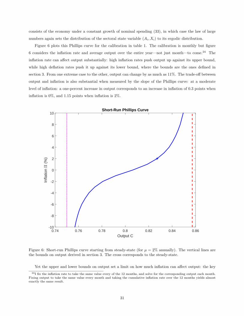
consists of the economy under a constant growth of nominal spending (33), in which case the law of large

numbers again sets the distribution of the sectoral state variable (Ai, Xi) to its ergodic distribution.

Figure 6 plots this Phillips curve for the calibration in table 1. The calibration is monthly but figure

6 considers the inflation rate and average output over the entire year—not just month—to come.24 The

inflation rate can affect output substantially: high inflation rates push output up against its upper bound,

while high deflation rates push it up against its lower bound, where the bounds are the ones defined in

section 3. From one extreme case to the other, output can change by as much as 11%. The trade-off between

output and inflation is also substantial when measured by the slope of the Phillips curve: at a moderate

level of inflation: a one-percent increase in output corresponds to an increase in inflation of 0.3 points when

inflation is 0%, and 1.15 points when inflation is 2%.

Output C0.74 0.76 0.78 0.8 0.82 0.84 0.86

Infla

tion &

(%

)

-10

-8

-6

-4

-2

0

2

4

6

8

10Short-Run Phillips Curve

Figure 6: Short-run Phillips curve starting from steady-state (for µ = 2% annually). The vertical lines arethe bounds on output derived in section 3. The cross corresponds to the steady-state.

Yet the upper and lower bounds on output set a limit on how much inflation can affect output: the key24I fix the inflation rate to take the same value every of the 12 months, and solve for the corresponding output each month.

Fixing output to take the same value every month and taking the cumulative inflation rate over the 12 months yields almostexactly the same result.

31

feature of the kinked-demand Phillips curve is its strong convexity for positive inflation rates, and strong

concavity for negative ones—all in all, the long-run Phillips curve is S-shaped. At 10% inflation, a one-

percent increase in output generates an increase in inflation of 7.2 percentage points. The convexity allows

to combine a rather flat Phillips curve at moderate rates of inflation with a virtually vertical one under

hyperinflation (and hyperdeflation). The convexity arises mechanically from the pricing function (31): small

increases in nominal marginal costs do not trigger much price increases as most firms do not reach the upper

end of their inaction regions, but for larger increases in costs many firms are pushed to the end of their

inaction regions and increase their prices.

The convexity of the kinked-demand Phillips curve is a constitutive property of the theory. Yet, it does

not necessarily set the theory apart. Indeed, on this account what first distinguishes the present model

from alternative theories of price rigidity is its tractability, which allows to easily solve for the Phillips curve

without relying on approximation methods. The norm in monetary models is to rely, often by necessity, on

linearizations methods, ruling out the possibility of investigating the extent of non-linearity in the Phillips

curve. Exceptions exist. Ball et al. (1988) consider a model of time-dependent pricing where firms set prices

for a deterministic, but endogenously chosen, amount of time. They find that firms choose a higher frequency

of price changes when inflation is higher, and that the slope of the Phillips curve increases with the inflation

rate. They present both features as properties of optimizing models of nominal rigidity, which endogenize

the extent of nominal rigidity. However, as the authors mention, if the higher frequency of price changes is

a robust feature which is for instance also predicted by state-dependent pricing menu-cost models (and, for

that matter, the present model), that the slope of the Phillips curve increases with inflation needs not follow.

The menu-cost model of Caplin and Spulber (1987), where money is completely neutral, offers a counter-

example, while the menu-cost model of Caplin and Leahy (1991, 1997), where monetary shocks impact output

differently depending on the level of output, suggests menu-costs models can generate non-linearities in the

Phillips curve. How convex a Phillips curve menu-cost models predict appears as an open question however,

because of the greater difficulty to solve menu-cost models.25 Akerlof et al. (2000) generate non-linearities

in the Phillips curve by considering near-rational agents who only incorporate inflation in their wage-setting

when inflation reaches a threshold of salience. In contrast, the convexity of the kinked-demand Phillips curve

does not rely on any departure from rationality.

The convexity of the kinked-demand Phillips curve provides simple explanations to some puzzles in the

evolution of the U.S. Phillips curve in the past decades. Atkeson and Ohanian (2001) document that the

slope of the Phillips curve is lower when estimated on the post early-1980s sample: the Phillips curve has

flattened.26 Some economists, such as Roberts (2006), have interpreted it as a consequence of changes in

monetary policy, which would have achieved a better anchoring of expectations. The convex kinked-demand

Phillips curve sees the decrease in the slope of the Phillips curve in the 1980s as exactly what one would25Menu-cost papers do not usually derive the Phillips curves of their models. The exception is Gertler and Leahy (2008).

They derive the Phillips curve of their model by relying on an approximation around steady-state however.26Stock and Watson (2009) survey the subsequent literature on Phillips curve inflation forecasts.

32

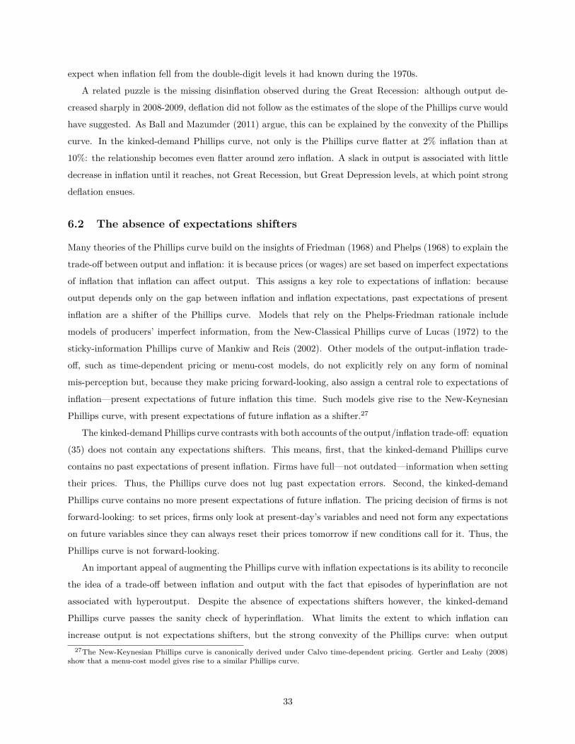
expect when inflation fell from the double-digit levels it had known during the 1970s.

A related puzzle is the missing disinflation observed during the Great Recession: although output de-

creased sharply in 2008-2009, deflation did not follow as the estimates of the slope of the Phillips curve would

have suggested. As Ball and Mazumder (2011) argue, this can be explained by the convexity of the Phillips

curve. In the kinked-demand Phillips curve, not only is the Phillips curve flatter at 2% inflation than at

10%: the relationship becomes even flatter around zero inflation. A slack in output is associated with little

decrease in inflation until it reaches, not Great Recession, but Great Depression levels, at which point strong

deflation ensues.

6.2 The absence of expectations shifters

Many theories of the Phillips curve build on the insights of Friedman (1968) and Phelps (1968) to explain the

trade-off between output and inflation: it is because prices (or wages) are set based on imperfect expectations

of inflation that inflation can affect output. This assigns a key role to expectations of inflation: because

output depends only on the gap between inflation and inflation expectations, past expectations of present

inflation are a shifter of the Phillips curve. Models that rely on the Phelps-Friedman rationale include

models of producers’ imperfect information, from the New-Classical Phillips curve of Lucas (1972) to the

sticky-information Phillips curve of Mankiw and Reis (2002). Other models of the output-inflation trade-

off, such as time-dependent pricing or menu-cost models, do not explicitly rely on any form of nominal

mis-perception but, because they make pricing forward-looking, also assign a central role to expectations of

inflation—present expectations of future inflation this time. Such models give rise to the New-Keynesian

Phillips curve, with present expectations of future inflation as a shifter.27

The kinked-demand Phillips curve contrasts with both accounts of the output/inflation trade-off: equation

(35) does not contain any expectations shifters. This means, first, that the kinked-demand Phillips curve

contains no past expectations of present inflation. Firms have full—not outdated—information when setting

their prices. Thus, the Phillips curve does not lug past expectation errors. Second, the kinked-demand

Phillips curve contains no more present expectations of future inflation. The pricing decision of firms is not

forward-looking: to set prices, firms only look at present-day’s variables and need not form any expectations

on future variables since they can always reset their prices tomorrow if new conditions call for it. Thus, the

Phillips curve is not forward-looking.

An important appeal of augmenting the Phillips curve with inflation expectations is its ability to reconcile

the idea of a trade-off between inflation and output with the fact that episodes of hyperinflation are not

associated with hyperoutput. Despite the absence of expectations shifters however, the kinked-demand

Phillips curve passes the sanity check of hyperinflation. What limits the extent to which inflation can

increase output is not expectations shifters, but the strong convexity of the Phillips curve: when output27The New-Keynesian Phillips curve is canonically derived under Calvo time-dependent pricing. Gertler and Leahy (2008)

show that a menu-cost model gives rise to a similar Phillips curve.

33

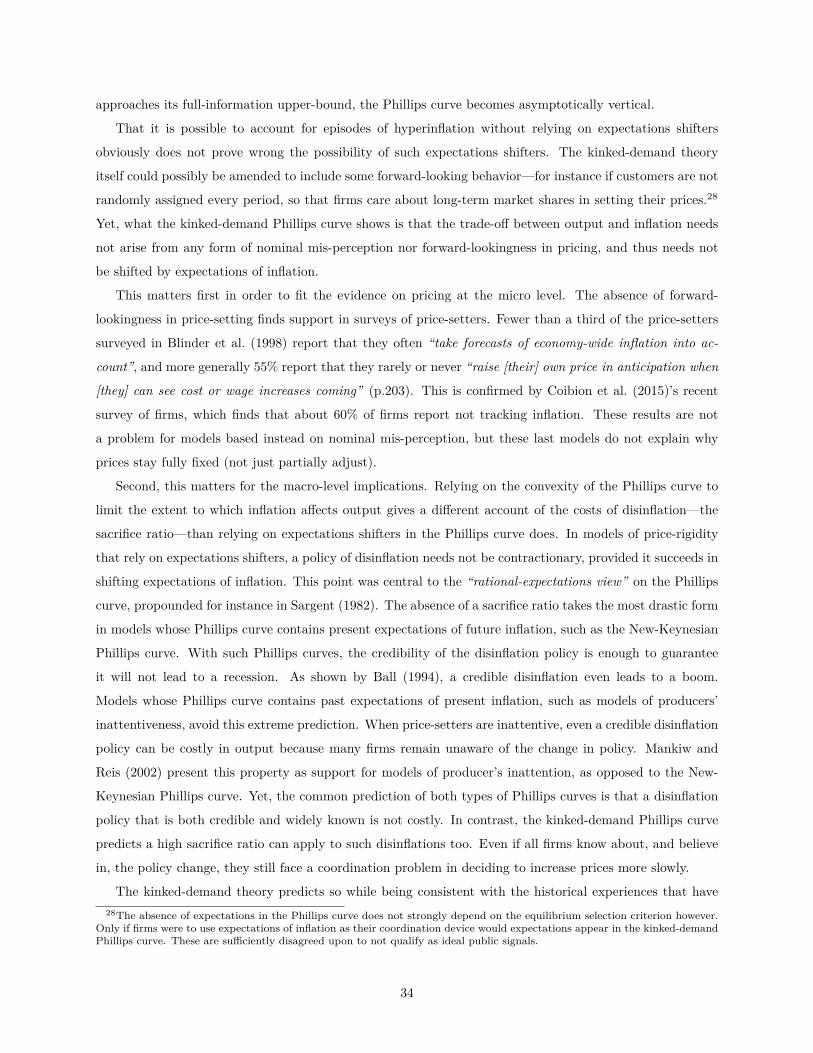
approaches its full-information upper-bound, the Phillips curve becomes asymptotically vertical.

That it is possible to account for episodes of hyperinflation without relying on expectations shifters

obviously does not prove wrong the possibility of such expectations shifters. The kinked-demand theory

itself could possibly be amended to include some forward-looking behavior—for instance if customers are not

randomly assigned every period, so that firms care about long-term market shares in setting their prices.28

Yet, what the kinked-demand Phillips curve shows is that the trade-off between output and inflation needs

not arise from any form of nominal mis-perception nor forward-lookingness in pricing, and thus needs not

be shifted by expectations of inflation.

This matters first in order to fit the evidence on pricing at the micro level. The absence of forward-

lookingness in price-setting finds support in surveys of price-setters. Fewer than a third of the price-setters

surveyed in Blinder et al. (1998) report that they often “take forecasts of economy-wide inflation into ac-

count”, and more generally 55% report that they rarely or never “raise [their] own price in anticipation when

[they] can see cost or wage increases coming” (p.203). This is confirmed by Coibion et al. (2015)’s recent

survey of firms, which finds that about 60% of firms report not tracking inflation. These results are not

a problem for models based instead on nominal mis-perception, but these last models do not explain why

prices stay fully fixed (not just partially adjust).

Second, this matters for the macro-level implications. Relying on the convexity of the Phillips curve to

limit the extent to which inflation affects output gives a different account of the costs of disinflation—the

sacrifice ratio—than relying on expectations shifters in the Phillips curve does. In models of price-rigidity

that rely on expectations shifters, a policy of disinflation needs not be contractionary, provided it succeeds in

shifting expectations of inflation. This point was central to the “rational-expectations view” on the Phillips

curve, propounded for instance in Sargent (1982). The absence of a sacrifice ratio takes the most drastic form

in models whose Phillips curve contains present expectations of future inflation, such as the New-Keynesian

Phillips curve. With such Phillips curves, the credibility of the disinflation policy is enough to guarantee

it will not lead to a recession. As shown by Ball (1994), a credible disinflation even leads to a boom.

Models whose Phillips curve contains past expectations of present inflation, such as models of producers’

inattentiveness, avoid this extreme prediction. When price-setters are inattentive, even a credible disinflation

policy can be costly in output because many firms remain unaware of the change in policy. Mankiw and

Reis (2002) present this property as support for models of producer’s inattention, as opposed to the New-

Keynesian Phillips curve. Yet, the common prediction of both types of Phillips curves is that a disinflation

policy that is both credible and widely known is not costly. In contrast, the kinked-demand Phillips curve

predicts a high sacrifice ratio can apply to such disinflations too. Even if all firms know about, and believe

in, the policy change, they still face a coordination problem in deciding to increase prices more slowly.

The kinked-demand theory predicts so while being consistent with the historical experiences that have28The absence of expectations in the Phillips curve does not strongly depend on the equilibrium selection criterion however.

Only if firms were to use expectations of inflation as their coordination device would expectations appear in the kinked-demandPhillips curve. These are sufficiently disagreed upon to not qualify as ideal public signals.

34

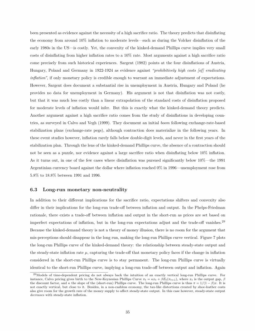
been presented as evidence against the necessity of a high sacrifice ratio. The theory predicts that disinflating

the economy from around 10% inflation to moderate levels—such as during the Volcker disinflation of the

early 1980s in the US—is costly. Yet, the convexity of the kinked-demand Phillips curve implies very small

costs of disinflating from higher inflation rates to a 10% rate. Most arguments against a high sacrifice ratio

come precisely from such historical experiences. Sargent (1982) points at the four disinflations of Austria,

Hungary, Poland and Germany in 1922-1924 as evidence against “prohibitively high costs [of] eradicating

inflation”, if only monetary policy is credible enough to warrant an immediate adjustment of expectations.

However, Sargent does document a substantial rise in unemployment in Austria, Hungary and Poland (he

provides no data for unemployment in Germany). His argument is not that disinflation was not costly,

but that it was much less costly than a linear extrapolation of the standard costs of disinflation proposed

for moderate levels of inflation would infer. But this is exactly what the kinked-demand theory predicts.

Another argument against a high sacrifice ratio comes from the study of disinflations in developing coun-

tries, as surveyed in Calvo and Vegh (1999). They document an initial boom following exchange-rate-based

stabilization plans (exchange-rate pegs), although contraction does materialize in the following years. In

these event studies however, inflation rarely falls below double-digit levels, and never in the first years of the

stabilization plan. Through the lens of the kinked-demand Phillips curve, the absence of a contraction should

not be seen as a puzzle, nor evidence against a large sacrifice ratio when disinflating below 10% inflation.

As it turns out, in one of the few cases where disinflation was pursued significantly below 10%—the 1991

Argentinian currency board against the dollar where inflation reached 0% in 1996—unemployment rose from

5.8% to 18.8% between 1991 and 1996.

6.3 Long-run monetary non-neutrality

In addition to their different implications for the sacrifice ratio, expectations shifters and convexity also

differ in their implications for the long-run trade-off between inflation and output. In the Phelps-Friedman

rationale, there exists a trade-off between inflation and output in the short-run as prices are set based on

imperfect expectations of inflation, but in the long-run expectations adjust and the trade-off vanishes.29

Because the kinked-demand theory is not a theory of money illusion, there is no room for the argument that

mis-perceptions should disappear in the long run, making the long-run Phillips curve vertical. Figure 7 plots

the long-run Phillips curve of the kinked-demand theory: the relationship between steady-state output and

the steady-state inflation rate µ, capturing the trade-off that monetary policy faces if the change in inflation

considered in the short-run Phillips curve is to stay permanent. The long-run Phillips curve is virtually

identical to the short-run Phillips curve, implying a long-run trade-off between output and inflation. Again29Models of time-dependent pricing do not always back the intuition of an exactly vertical long-run Phillips curve. For

instance, Calvo pricing gives birth to the New-Keynesian Phillips Curve πt = κxt + βEt(πt+1), where xt is the output gap, βthe discount factor, and κ the slope of the (short-run) Phillips curve. The long-run Phillips curve is thus π = 1/(1− β)x. It isnot exactly vertical, but close to it. Besides, in a non-cashless economy, the tax-like distortions created by shoe-leather costsalso give room for the growth rate of the money supply to affect steady-state output. In this case however, steady-state outputdecreases with steady-state inflation.

35

however, this trade-off is limited by the strong convexity of the Phillips curve. In the kinked-demand theory,

it is not that the Phillips curve is flat in the short-run and vertical in the long-run. Instead, it is flat at low

levels of inflation, and vertical at high levels.30

Output C0.74 0.76 0.78 0.8 0.82 0.84 0.86

Infla

tion &

(%

)

-10

-8

-6

-4

-2

0

2

4

6

8

10Long-Run and Short-Run Phillips Curve

Short-Run PCLong-Run PC

Figure 7: Long-run Phillips curve, superimposed on the short-run Phillips curve. The vertical lines are thebounds on output derived in section 3. The cross corresponds to the µ = 2% steady-state.

A higher inflation target increases output persistently because it persistently affects the position of firms

within their inaction regions. The upper panel of figure 8 plots, for annual inflation rates of −2% to 2%,

the cross-sectional distribution of the Xi’s within the inaction region. Higher inflation shifts the distribution

of the Xi’s to the right. As a consequence, the distribution of markups shifts to the left, as shown in the

bottom panel. (The bottom panel plots the distribution of Pi/W instead of the distribution of markups

Pi/WAi because the two masses inM(α+ θ) andM(α(1− λ) + θ) in the distribution of markups makes it

hard to visualize.) As markups decrease, output increases.30The model of Akerlof et al. (2000) yields a similar property. In their model with near-rational agents, it is not that agents

face money illusion in the short-run and not in the long-run, but instead that agents face money illusion at low inflationrates and not high inflation rates. In contrast to Akerlof et al. (2000), the kinked-demand theory departs altogether from theinterpretation of the output/inflation trade-off as a mis-perception between real and nominal variables (and does not rely onany departure from rationality).

36

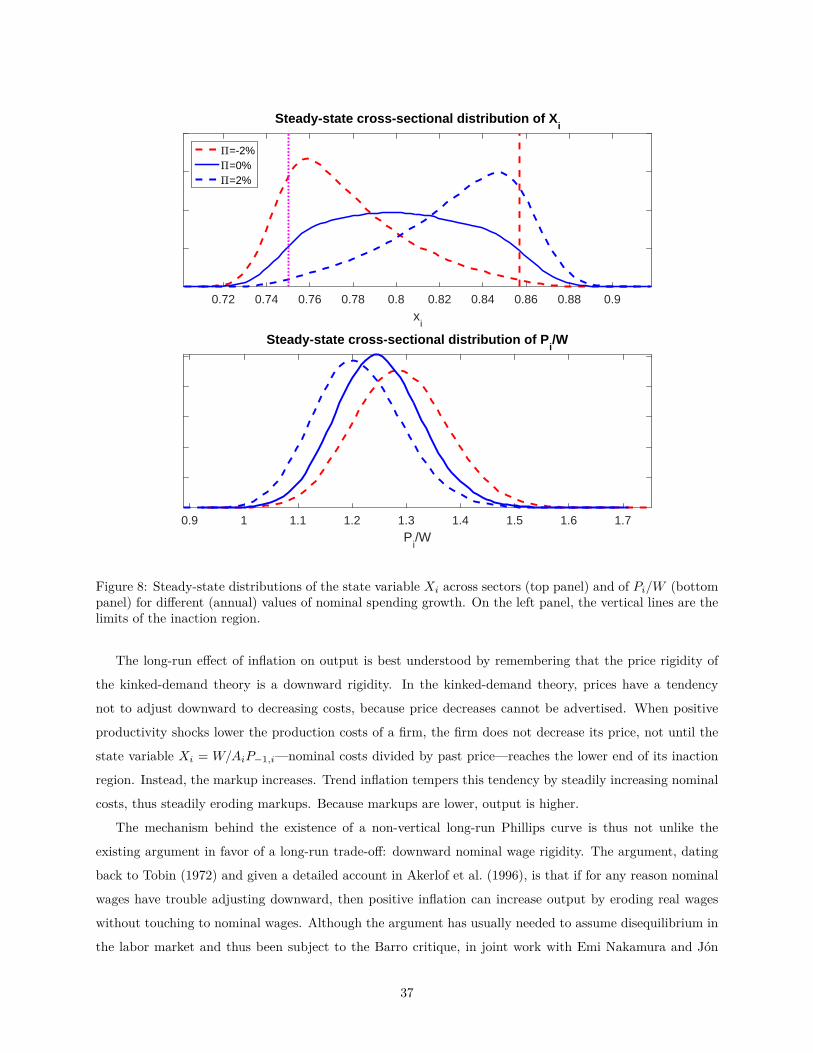
xi

0.72 0.74 0.76 0.78 0.8 0.82 0.84 0.86 0.88 0.9

Steady-state cross-sectional distribution of Xi

&=-2%&=0%&=2%

Pi/W

0.9 1 1.1 1.2 1.3 1.4 1.5 1.6 1.7

Steady-state cross-sectional distribution of Pi/W

Figure 8: Steady-state distributions of the state variable Xi across sectors (top panel) and of Pi/W (bottompanel) for different (annual) values of nominal spending growth. On the left panel, the vertical lines are thelimits of the inaction region.

The long-run effect of inflation on output is best understood by remembering that the price rigidity of

the kinked-demand theory is a downward rigidity. In the kinked-demand theory, prices have a tendency

not to adjust downward to decreasing costs, because price decreases cannot be advertised. When positive

productivity shocks lower the production costs of a firm, the firm does not decrease its price, not until the

state variable Xi = W/AiP−1,i—nominal costs divided by past price—reaches the lower end of its inaction

region. Instead, the markup increases. Trend inflation tempers this tendency by steadily increasing nominal

costs, thus steadily eroding markups. Because markups are lower, output is higher.

The mechanism behind the existence of a non-vertical long-run Phillips curve is thus not unlike the

existing argument in favor of a long-run trade-off: downward nominal wage rigidity. The argument, dating

back to Tobin (1972) and given a detailed account in Akerlof et al. (1996), is that if for any reason nominal

wages have trouble adjusting downward, then positive inflation can increase output by eroding real wages

without touching to nominal wages. Although the argument has usually needed to assume disequilibrium in

the labor market and thus been subject to the Barro critique, in joint work with Emi Nakamura and Jón

37

Steinsson (Dupraz et al. (2016)) we show that a labor search framework makes it consistent with equilibrium

and robust to the Barro critique.

Here prices, not wages, are the sticky ones. But here too inflation acts by having relative prices adjust

in a way they would not without the help of inflation: inflation greases the wheels of the goods market.

There is a substantial difference however: the reasons for the lack of adjustment in the absence of inflation

is different. The downward rigidity of nominal wages is usually argued to come from psychological barriers

to wage cuts combined with money illusion. Here there is neither money illusion nor loss aversion. Instead,

the problem is a coordination failure: a firm has no incentive to adjust its price after a shock if it is the only

firm to do so. Inflation makes the adjustment for everyone at once.

The existence of a non-vertical long-run Phillips curve has long been a contentious empirical issue.

Traditional tests—assessing whether the coefficients on lagged inflations sum to one—fell out of fashion after

Sargent (1971) pointed out that identifying the slope of the long-run Phillips curve in this way requires to

assume that inflation expectations load one for one on past inflation, a strong assumption given that inflation

had been little serially correlated historically. However, King and Watson (1994) show that the slope of the

long-run Phillips is identified provided inflation has a unit root, and find this slope to be non-vertical when

using a structural VAR with a Keynesian identification. Yet, using a higher-dimensional VAR and different

identification assumptions, Benati (2015) cannot reject the hypothesis of a vertical long-run Phillips curve.

As Benati stresses, the incontrovertible result is the substantial uncertainty surrounding the estimates: at

bottom the problem is that there is little information in the existing data to estimate the slope of the

long-run Phillips curve, both because of the generic difficulty in estimating the long-run, and because of the

need to rely only on the permanent variations in inflation. If the empirical evidence is inconclusive, what

the kinked-demand theory shows is that there is no theoretical basis to exclude the possibility of a long-run

trade-off as inconsistent with rationality or rational expectations.

The existence of a long-run trade-off between inflation and output summons the normative question:

should monetary policy exploit it by targeting a higher inflation target? The benefit of a higher inflation

target implied by the kinked-demand theory—eroding markups—adds to the two main arguments in favor

of higher inflation targets: greasing the wheels of the labor markets by eroding real wages when nominal

wages are downwardly rigid, as already mentioned, and creating a buffer away from the liquidity trap.31

Pinning down the optimal inflation target called for by the possibility of eroding markups requires to

compare this new benefit to the costs of inflation. The present version of the model does incorporates the one

cost of inflation usually taken into account in studies of optimal monetary policy (Woodford (2003a)): the

welfare loss stemming from possibly more dispersed relative prices. Yet, in the model higher inflation does

not increase relative price dispersion within markets. Thus, the optimal inflation rate is trivially infinite.

The absence of connection between inflation and price dispersion is confirmed empirically in Nakamura and

Steinsson (2016). As they stress, it is thus still unclear what the relevant costs of inflation are and how to31The case for a positive inflation target to avoid falling in the liquidity trap is often attributed to Summers (1991).

38

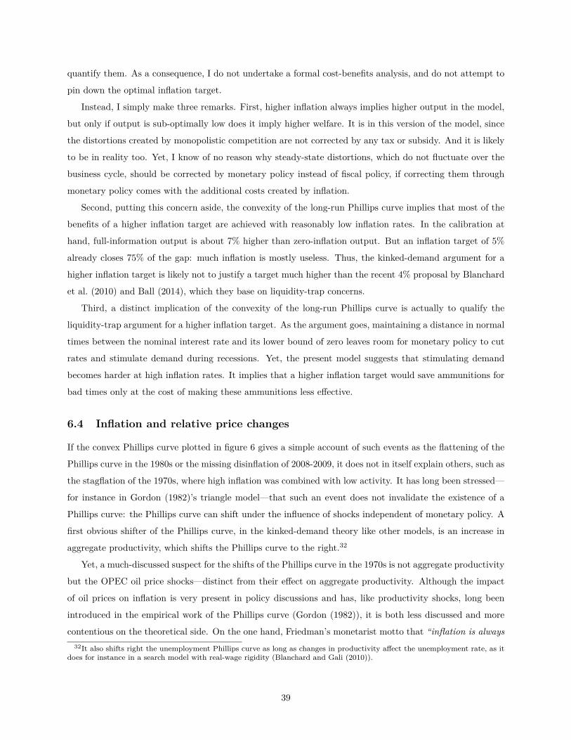
quantify them. As a consequence, I do not undertake a formal cost-benefits analysis, and do not attempt to

pin down the optimal inflation target.

Instead, I simply make three remarks. First, higher inflation always implies higher output in the model,

but only if output is sub-optimally low does it imply higher welfare. It is in this version of the model, since

the distortions created by monopolistic competition are not corrected by any tax or subsidy. And it is likely

to be in reality too. Yet, I know of no reason why steady-state distortions, which do not fluctuate over the

business cycle, should be corrected by monetary policy instead of fiscal policy, if correcting them through

monetary policy comes with the additional costs created by inflation.

Second, putting this concern aside, the convexity of the long-run Phillips curve implies that most of the

benefits of a higher inflation target are achieved with reasonably low inflation rates. In the calibration at

hand, full-information output is about 7% higher than zero-inflation output. But an inflation target of 5%

already closes 75% of the gap: much inflation is mostly useless. Thus, the kinked-demand argument for a

higher inflation target is likely not to justify a target much higher than the recent 4% proposal by Blanchard

et al. (2010) and Ball (2014), which they base on liquidity-trap concerns.

Third, a distinct implication of the convexity of the long-run Phillips curve is actually to qualify the

liquidity-trap argument for a higher inflation target. As the argument goes, maintaining a distance in normal

times between the nominal interest rate and its lower bound of zero leaves room for monetary policy to cut

rates and stimulate demand during recessions. Yet, the present model suggests that stimulating demand

becomes harder at high inflation rates. It implies that a higher inflation target would save ammunitions for

bad times only at the cost of making these ammunitions less effective.

6.4 Inflation and relative price changes

If the convex Phillips curve plotted in figure 6 gives a simple account of such events as the flattening of the

Phillips curve in the 1980s or the missing disinflation of 2008-2009, it does not in itself explain others, such as

the stagflation of the 1970s, where high inflation was combined with low activity. It has long been stressed—

for instance in Gordon (1982)’s triangle model—that such an event does not invalidate the existence of a

Phillips curve: the Phillips curve can shift under the influence of shocks independent of monetary policy. A

first obvious shifter of the Phillips curve, in the kinked-demand theory like other models, is an increase in

aggregate productivity, which shifts the Phillips curve to the right.32

Yet, a much-discussed suspect for the shifts of the Phillips curve in the 1970s is not aggregate productivity

but the OPEC oil price shocks—distinct from their effect on aggregate productivity. Although the impact

of oil prices on inflation is very present in policy discussions and has, like productivity shocks, long been

introduced in the empirical work of the Phillips curve (Gordon (1982)), it is both less discussed and more

contentious on the theoretical side. On the one hand, Friedman’s monetarist motto that “inflation is always32It also shifts right the unemployment Phillips curve as long as changes in productivity affect the unemployment rate, as it

does for instance in a search model with real-wage rigidity (Blanchard and Gali (2010)).

39

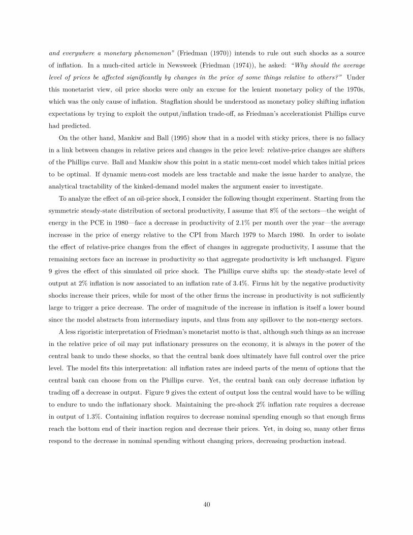
and everywhere a monetary phenomenon” (Friedman (1970)) intends to rule out such shocks as a source

of inflation. In a much-cited article in Newsweek (Friedman (1974)), he asked: “Why should the average

level of prices be affected significantly by changes in the price of some things relative to others?” Under

this monetarist view, oil price shocks were only an excuse for the lenient monetary policy of the 1970s,

which was the only cause of inflation. Stagflation should be understood as monetary policy shifting inflation

expectations by trying to exploit the output/inflation trade-off, as Friedman’s accelerationist Phillips curve

had predicted.

On the other hand, Mankiw and Ball (1995) show that in a model with sticky prices, there is no fallacy

in a link between changes in relative prices and changes in the price level: relative-price changes are shifters

of the Phillips curve. Ball and Mankiw show this point in a static menu-cost model which takes initial prices

to be optimal. If dynamic menu-cost models are less tractable and make the issue harder to analyze, the

analytical tractability of the kinked-demand model makes the argument easier to investigate.

To analyze the effect of an oil-price shock, I consider the following thought experiment. Starting from the

symmetric steady-state distribution of sectoral productivity, I assume that 8% of the sectors—the weight of

energy in the PCE in 1980—face a decrease in productivity of 2.1% per month over the year—the average

increase in the price of energy relative to the CPI from March 1979 to March 1980. In order to isolate

the effect of relative-price changes from the effect of changes in aggregate productivity, I assume that the

remaining sectors face an increase in productivity so that aggregate productivity is left unchanged. Figure

9 gives the effect of this simulated oil price shock. The Phillips curve shifts up: the steady-state level of

output at 2% inflation is now associated to an inflation rate of 3.4%. Firms hit by the negative productivity

shocks increase their prices, while for most of the other firms the increase in productivity is not sufficiently

large to trigger a price decrease. The order of magnitude of the increase in inflation is itself a lower bound

since the model abstracts from intermediary inputs, and thus from any spillover to the non-energy sectors.

A less rigoristic interpretation of Friedman’s monetarist motto is that, although such things as an increase

in the relative price of oil may put inflationary pressures on the economy, it is always in the power of the

central bank to undo these shocks, so that the central bank does ultimately have full control over the price

level. The model fits this interpretation: all inflation rates are indeed parts of the menu of options that the

central bank can choose from on the Phillips curve. Yet, the central bank can only decrease inflation by

trading off a decrease in output. Figure 9 gives the extent of output loss the central would have to be willing

to endure to undo the inflationary shock. Maintaining the pre-shock 2% inflation rate requires a decrease

in output of 1.3%. Containing inflation requires to decrease nominal spending enough so that enough firms

reach the bottom end of their inaction region and decrease their prices. Yet, in doing so, many other firms

respond to the decrease in nominal spending without changing prices, decreasing production instead.

40

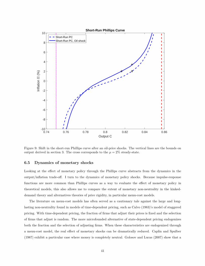
Output C0.74 0.76 0.78 0.8 0.82 0.84 0.86

Infla

tion &

(%

)

-10

-8

-6

-4

-2

0

2

4

6

8

10Short-Run Phillips Curve

Short-Run PCShort-Run PC, Oil shock

Figure 9: Shift in the short-run Phillips curve after an oil-price shocks. The vertical lines are the bounds onoutput derived in section 3. The cross corresponds to the µ = 2% steady-state.

6.5 Dynamics of monetary shocks

Looking at the effect of monetary policy through the Phillips curve abstracts from the dynamics in the

output/inflation trade-off. I turn to the dynamics of monetary policy shocks. Because impulse-response

functions are more common than Phillips curves as a way to evaluate the effect of monetary policy in

theoretical models, this also allows me to compare the extent of monetary non-neutrality in the kinked-

demand theory and alternatives theories of price rigidity, in particular menu-cost models.

The literature on menu-cost models has often served as a cautionary tale against the large and long-

lasting non-neutrality found in models of time-dependent pricing, such as Calvo (1983)’s model of staggered

pricing. With time-dependent pricing, the fraction of firms that adjust their prices is fixed and the selection

of firms that adjust is random. The more microfounded alternative of state-dependent pricing endogenizes

both the fraction and the selection of adjusting firms. When these characteristics are endogenized through

a menu-cost model, the real effect of monetary shocks can be dramatically reduced. Caplin and Spulber

(1987) exhibit a particular case where money is completely neutral. Golosov and Lucas (2007) show that a

41

more realistic version of the menu-cost model, which adds in particular idiosyncratic shocks, predicts, if no

complete neutrality, very transient effects of monetary shocks.

State-dependent pricing is often used as a synonym for menu-cost models. Yet it is not: the kinked

demand curve theory is a model of state-dependent pricing too. I show that the kinked-demand theory

predicts much longer-lived real effects of monetary shocks than in the benchmark menu-cost model of Golosov

and Lucas (2007), and thus that the transient effects of monetary shocks in menu-cost models is not a

general feature of state-dependent pricing, but only of the specific way menu-cost models make pricing

state-dependent.

I use Golosov and Lucas’s results as a comparison point to contrast the predictions of the kinked-demand

theory with the predictions of menu-cost models. To be sure, the model of Golosov and Lucas is only a

particular version of the menu-cost framework. In particular, it considers a case with no strategic comple-

mentarity in price-setting. Subsequent literature—for instance Gertler and Leahy (2008) and Nakamura and

Steinsson (2010)—has shown that strategic complementarities amplify the real effect of monetary shocks in

menu-cost models just as it does in models of time-dependent pricing. But the version of the kinked-demand

model I consider in this paper shares the same sin as Golosov and Lucas’s model: insofar as strategic com-

plementarities are measured by the slope of the notional short-run aggregate supply (SRAS), there is none.

Golosov and Lucas’s model is thus the appropriate benchmark.

To evaluate the extent of short-run monetary non-neutrality, I run the same experiment as the one

Golosov and Lucas use to show the transient effects of monetary shocks in their benchmark menu-cost

model: starting at the steady-state, I simulate a one-time 1% increase in nominal spending and look at how

output responds.33 Figure 11 plots the quarterly impulse-response function of output when the inflation

target µ is 2%. On impact, most of the increase in nominal spending translates into an increase in output.

More critically, the shock is much more persistent than in Golosov and Lucas (2007)’s menu-cost model.

There, all effects of the monetary shock disappear in about half-a-quarter; here, the effect of the shock is still

about 40% of its initial impact after a year, and 20 % after two. The persistence of the shock is much more

in line with the persistence predicted by the Calvo model. Figure 11 superimposes the impulse-response for

the Calvo model, absent strategic complementarities 34

What accounts for the difference between the kinked-demand theory and a menu-cost model? Both in

a menu-cost model and in the kinked-demand theory, the firms that are triggered to increase their prices

following a positive monetary shock are the ones that are at the upper end of their inaction region. What

differs is the connection between the size of cost-changes and the size of price-changes discussed in section

5.3. In a menu-cost model, a firm makes a large price-adjustment regardless of the size of the cost-shock.33Because behavior is derived under the expectation of no shock, the questions arises of whether this is consistent with rational

expectations. A general argument to answer yes, which applies to both the menu-cost and the kinked-demand models, is thatzero-probability events can happen. An argument specific to the kinked-demand model is that the expectations of price-setterson the process for costs do not matter anyway: price-setting is not forward-looking.

34Specifically, this is the IRF implied by the log-linearized New-Keynesian Phillips curve πt = κxt + βEt(πt+1), whereκ = (1− ξ)(1− βξ)/ξ, with ξ the probability of not resetting prices calibrated to ξ = 8/9—a price duration of 9 months—andβ the discount factor calibrated to β = 0.99.

42

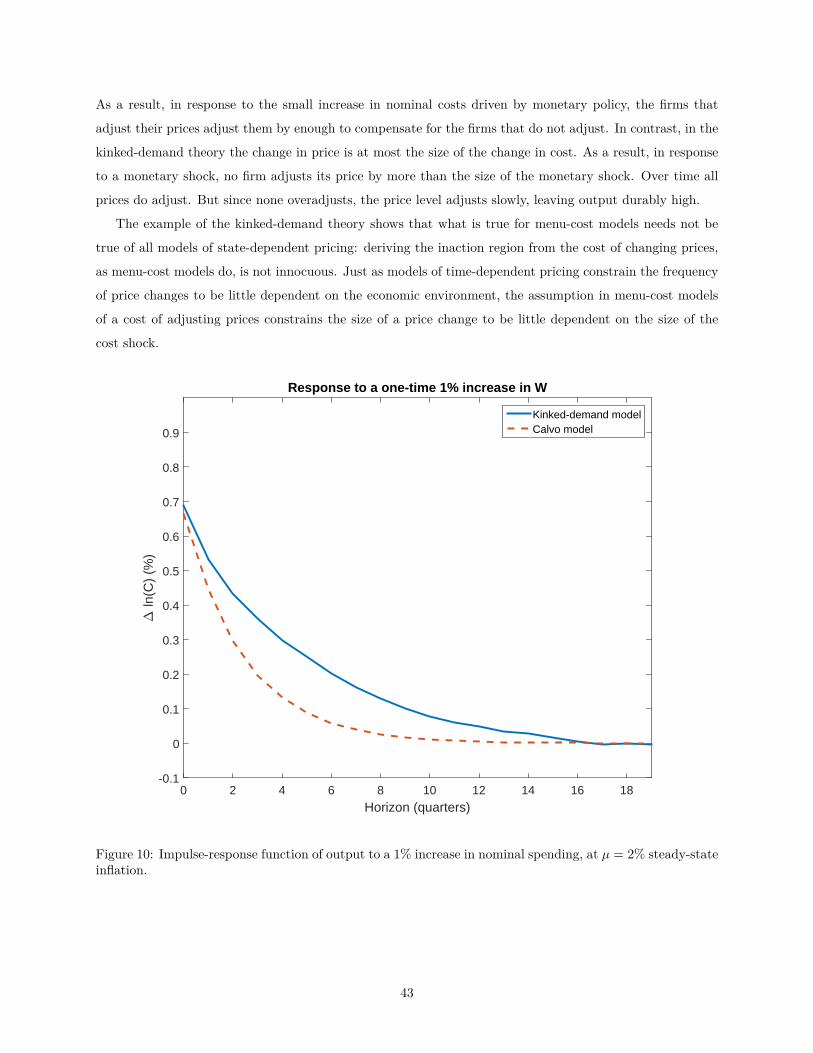
As a result, in response to the small increase in nominal costs driven by monetary policy, the firms that

adjust their prices adjust them by enough to compensate for the firms that do not adjust. In contrast, in the

kinked-demand theory the change in price is at most the size of the change in cost. As a result, in response

to a monetary shock, no firm adjusts its price by more than the size of the monetary shock. Over time all

prices do adjust. But since none overadjusts, the price level adjusts slowly, leaving output durably high.

The example of the kinked-demand theory shows that what is true for menu-cost models needs not be

true of all models of state-dependent pricing: deriving the inaction region from the cost of changing prices,

as menu-cost models do, is not innocuous. Just as models of time-dependent pricing constrain the frequency

of price changes to be little dependent on the economic environment, the assumption in menu-cost models

of a cost of adjusting prices constrains the size of a price change to be little dependent on the size of the

cost shock.

Horizon (quarters)0 2 4 6 8 10 12 14 16 18

" ln

(C)

(%)

-0.1

0

0.1

0.2

0.3

0.4

0.5

0.6

0.7

0.8

0.9

Response to a one-time 1% increase in W

Kinked-demand modelCalvo model

Figure 10: Impulse-response function of output to a 1% increase in nominal spending, at µ = 2% steady-stateinflation.

43

7 Conclusion

When it comes to sticky prices, economists and practitioners tend to disagree. Practitioners perceive price-

rigidity as the optimal response to the demand curves they face. We economists rely on models where

demand curves predict flexible desired prices, and assimilate price-rigidity to firms’ inability to track these

desired prices.

In this paper, I have argued that theory needs not contradict the perception of practitioners. I have

shown that the oldest of customer-side theories of price rigidity—the kinked demand-curve theory—is as

consistent with optimizing behavior, equilibrium, and rational expectations, as firm-side theories are. I

have pointed at ways by which deciding between the theories can be moved from price-setters’ surveys to

microdata empirical studies. And I have shown that the question matters: the kinked-demand theory has

implications for monetary policy that substantially differ from the ones of firm-side models.

I conclude by pointing at a last implication of the kinked-demand theory I have not touched here. The key

assumption that gives the kinked-demand curve in this paper is that not all consumers know about all prices

in a market. Information is endogenous in the model: uninformed customers decide whether to move to

competitors and learn their prices. Yet, throughout the paper I have maintained the fraction of uninformed

customers as exogenous. It can be endogenized: by considering firms’ decision to inform customers, the

kinked-demand theory naturally lends itself to a theory of advertising at business-cycle frequency.

44

A Proof of the existence of the equilibrium under full information

To complete the proof that all firms charging Pi =M(α+ θ)W/Ai is indeed an equilibrium, I need to check

that when all firms charge Pi, firm k’s profits have a global—not just local—optimum at P k = Pi. Under

the assumption of a Pareto distribution for F , for P k ≥ Pi firm k faces a constant-elastic demand curve with

elasticity α + θ, and it is easy to check that the derivative of profits is negative over P k > Pi. The more

involved verification is to check that profits are increasing over P k < Pi. Equivalently, using the relative

price p = P k/Pi and noting c = W/AiPi = 1M(α+θ) , I need to check that:

(p− c) (2− pα)p−θ (36)

is increasing over p < 1. The derivative of (36) has the sign of:

G(p) = (2− pα) +(

1− c

p

)(−αpα − θ(2− pα)). (37)

Both term are strictly positive for p < c, but the second term is negative for p > c. In this case however,

since 1− cp < 1− c = 1

α+θ :

G(p) > (2− pα) + 1α+ θ

(−αpα − θ(2− pα)) = 2(1− pα) α

α+ θ> 0, (38)

which ends the proof.

B Proof of the existence of the equilibrium under asymmetric

information

The proof is the same as the one under full information of the previous appendix. For P k ≥ Pi firm k, faces

a constant-elastic demand curve with elasticity α+ θ, and the derivative of profits is negative over P k > Pi.

To show profits are increasing for P k < Pi, it is equivalent to show, noting p = P k/Pi and c = W/AiPi,

that:

(p− c) [λ+ (1− λ)(2− pα)]p−θ (39)

is increasing over p < 1. The derivative of (39) has the sign of:

G(p) =(

2− λ− (1− λ)pα)

+(

1− c

p

)(− α(1− λ)pα − θ

[2− λ− (1− λ)pα

]). (40)

45

Both term are strictly positive for p < c, but the second term is negative for p > c. In this case however,

since 1− cp < 1− c ≤ 1− 1

M((1−λ)α+θ) = 1(1−λ)α+θ :

G(p) >(

2− λ− (1− λ)pα)

+ 1(1− λ)α+ θ

(− α(1− λ)pα − θ

[2− λ− (1− λ)pα

])= (2− λ)(1− pα) α(1− λ)

α(1− λ) + θ> 0,

(41)

which ends the proof.

C Characterization of the adaptive rational-expectations equilib-

rium

First, I derive firm k’s best-response to any market price Pi it expects. (This in effect extends the problem

treated in section 3, where Pi was restricted to be an equilibrium price; now it can be any price.) Firm

k still maximizes present profits πk =(P k − W

Ai

)Dk(P k). There are three cases. First, if the optimal

response P k is greater than Pi, firm k faces a demand curve with constant elasticity α+ θ around P k, and

sets P k = M(α + θ)WAi . This occurs when Pi ≤ M(α + θ)WAi . Second is the case P k = Pi, treated in

section 3. As seen there, this occurs when Pi ∈ [M(θ + α)W/Ai,M(θ + α(1 − λ))W/Ai], then firm k sets

P k = Pi. Finally, if P k is less than Pi, profits are differentiable at P k and the optimal P k is determined by

the first-order condition again. It solves:

−(

1− W

AiP k

)[θ

((1− λ)

(2−

(P k

Pi

)α)+ λ

)+ α(1− λ)

(P k

Pi

)α]+ (1− λ)

(2−

(P k

Pi

)α)+ λ = 0.

(42)

which implicitly defines the best-response P k as a function of Pi. The function is only implicit, but the

contrapositive of the two previous cases guarantees that this last case occurs when Pi ≥M(θ+α(1−λ))W/Ai,

completing the partition of mutually exclusive cases. Taken together, the three cases define, for any given

value of W/Ai, the best-response price P k to any price Pi. It is illustrated in figure 11.

This best-response function defines the sequence (Ps)s≥0 of mental iterations, starting from the initial

value P0 = P−1,i, the market price in the past period. Consider now the price to which the iterative

process converges. Again, distinguish three cases. If P0 = P−1,i ≤ M(α + θ)WAi—the case when the

past price is too low for equilibrium—firms set Pk = M(α + θ)WAi in the first round of the iteration,

which is an equilibrium price: the process stops at round 2 with Pi = M(α + θ)WAi : a price increase. If

P0 = P−1,i ∈ [M(θ + α)W/Ai,M(θ + α(1− λ))W/Ai]—the case when the past price is still consistent with

equilibrium—firms set P k = P−1,i in the first round of iteration: the process stops at round 1 and firms

keep their prices fixed Pi = P−1,i. Finally, if P−1,i ≥ M(θ + α(1 − λ))W/Ai—the case when the past

price is too low for equilibrium—then the process defines a strictly decreasing sequence that remains within

46

Pi

Pk

M(,+3) W/Ai

M(,(1-6)+3) W/Ai

Best-response Pk to a market price Pi

45° lineBest-response

Figure 11: Best-response P k to a market-price Pi. Calibration: α = 6, θ = 1, and λ = 1/2.

[M(θ+α(1− λ))W/Ai,+∞). By the monotone convergence theorem, the iterative process converges (in an

infinity of rounds) to the unique possible fixed point Pi =M(θ + α(1− λ))W/Ai: a price decrease.

47

ReferencesAkerlof, G., Dickens, W., and Perry, G. (1996). The macroeconomics of low inflation. Brookings Papers onEconomic Activity, (1):1–59.

Akerlof, G., Dickens, W., and Perry, G. (2000). Near-rational wage and price setting and the long-run phillipscurve. Brookings Papers on Economic Activity, (1):1–60.

Alvarez, F., Lippi, F., and Pacielllo, L. (2011). Optimal price setting with observation and menu costs.Quarterly Journal of Economics, 126(4):100–124.

Amirault, D., Kwan, C., and Wilkinson, G. (2004). A survey of the price-setting behavior of canadiancompanies. Bank of Canada Review, pages 29–40.

Apel, M., Friberg, R., and Hallsten, K. (2005). Microfoundations of macroeconomic price adjustment: surveyevidence from swedish firms. Journal of Money, Credit and Banking, 37(2):313–338.

Atkeson, A. and Ohanian, L. (2001). Are phillips curves useful for forecasting inflation. Quarterly Review,Federal Reserve Bank of Minneapolis, 25(1):2–11.

Ball, L. (1994). Credible disinflation with staggered price-setting. American Economic Review, 84(1):282–289.

Ball, L. (2014). The case for a long-run inflation target of four percent. mimeo.

Ball, L. and Mankiw, G. (1994). A sticky-price manifesto. Carnegie-Rochester Conference Series on PublicPolicy, 41:127–151.

Ball, L., Mankiw, G., and Romer, D. (1988). The new keynesian economics and the output-inflation trade-off.Brookings Papers on Economic Activity, (1):1–82.

Ball, L. and Mazumder, S. (2011). Inflation dynamics and the great recession. Brookings Papers on EconomicActivity, Spring:337–405.

Ball, L. and Romer, D. (1991). Sticky prices and coordination failure. American Economic Review, 81(3):539–552.

Benabou, R. and Gertner, R. (1993). Search with learning from prices: Does increased inflationary uncer-tainty leads to higher markups. Review of Economic Studies, 60(1):69–93.

Benati, L. (2015). The long-run phillips curve: A structural var investigation. Journal of Monetary Eco-nomics, 76.

Bernheim, D. (1984). Rationalizable strategic behavior. Econometrica, 52:1007–1028.

Binmore, K. (1987). Modeling rational players: Part 1. Economics and Philosophy, 3:179–214.

Blanchard, O., Dell’Ariccia, G., and Mauro, P. (2010). Rethinking macroeconomic policy. IMF Staff PositionNote.

Blanchard, O. and Gali, J. (2010). Labor markets and monetary policy: A new keynesian model withunemployment. American Economic Journal: A New Keynesian Model with Unemployment, 2(2):1–30.

Blinder, A. (1991). Why are prices sticky? preliminary results form an interview study. American EconomicReview, 81(2):89–96.

48

Blinder, A., Canetti, E., Lebow, D., and Rudd, J. (1998). Asking about prices, a new approach to understandprice stickiness. Russell Sage Foundation.

Braverman, A. (1980). Consumer search and alternative market equilibria. Review of Economic Studies,47:487–502.

Caballero, R. and Engel, E. (1991). Dynamic (s,s) economies. Econometrica, 59(6):1659–1686.

Caballero, R. and Engel, E. (1993). Heterogeneity and output fluctuations in a dynamic menu-cost economy.Review of Economic Studies, 60(1):95–119.

Calvo, G. (1983). Staggered prices in a utility-maximizing framework. Journal of Monetary Economics,12:383–398.

Calvo, G. and Vegh, C. (1999). Inflation stabilization and bop crises in developing countries. chapter 24,pages 1531–1614. Elsevier Science B.V.

Campbell, J. and Eden, B. (2014). Rigid prices: Evidence from u.s. scanner data. International EconomicReview, 55(2):423–442.

Caplin, A. and Leahy, J. (1991). State-depedent pricing and the dynamics of money and output. QuarterlyJournal of Economics, 106(3):683–708.

Caplin, A. and Leahy, J. (1997). Aggregation and optimization with state-dependent pricing. Econometrica,65(3):601–625.

Caplin, A. and Spulber, D. (1987). Menu costs and the neutrality of money. Quarterly Journal of Economics,102(4):703–726.

Cavallo, A. (2016a). The billion prices project: Using online data for measurement and research. Journal ofEconomic Perspectives, fothcoming.

Cavallo, A. (2016b). Scraped data and sticky prices. mimeo.

Cavallo, A. and Rigobon, R. (2011). The distribution of the size of price changes. mimeo.

Coibion, O., Gorodnichenko, Y., and Kumar, S. (2015). How do firms form their expectations? new surveyevidence. mimeo.

Dana, J. (1994). Learning in an equilibrium search model. International Economics Review, 35(3):745–771.

Danziger, L. (1999). A dynamic economy with costly price adjustments. American Economy Review,89(4):878–901.

Danziger, M. and King, R. (2005). Implications of state-dependent pricing for dynamic macroeconomicmodels. Journal of Monetary Economics, 52:213–242.

Dotsey, M., King, R., and Wolman, A. (1999). State-dependent pricing and the general equilibrium dynamicsof money and output. Quarterly Journal of Economics, 114(2):655–690.

Dupraz, S. (2016). Search models and kinked demands. mimeo.

Dupraz, S., Nakamura, E., and Steinsson, J. (2016). A plucking model of business cycles. mimeo.

Efroymson, C. (1943). A note on kinked demand curves. American Economic Review, 33(1):98–109.

49

Eichenbaum, M., Jaimovich, N., and Rebelo, S. (2011). Reference prices, costs, and nominal rigidities.American Economic Review, 101(1):234–262.

Eichenbaum, M., Jaimovich, N., Rebelo, S., and Smith, J. (2014). How frequent are small price changes.American Economic Journal: Macroeconomics, 6(2):137–155.

Evans, G. and Ramey, G. (1992). Expectation calculation and and macroeconomic dynamics. AmericanEconomic Review, 82(1):207–224.

Fabiani, S., Loupias, C., Martins, F., and Sabbatini, R. (2007). Pricing Decisions in the Euro Area: HowFirms Set Prices and Why. Oxford University Press.

Farrell, J. and Klemperer, P. (2007). Coordination and lock-in: competition with switching costs and networkeffects. In Amstrong, M. and Porter, R., editors, Handbook of Industrial Organization, volume 3. Elsevier.

Fishman, A. (1996). Search with learning and price adjustment dynamics. Quarterly Journal of Economics,111(1):253–268.

Foster, L., Haltiwanger, J., and Syverson, C. (2008). Reallocation, firm turnover, and efficiency: Selectionon productivity or profitability? American Economic Review, 98(1):394–425.

Friedman, M. (1968). The role of monetary policy. American Economic Review, 58(1):1–17.

Friedman, M. (1970). The counter-revolution in monetary theory. IEA Occasional Paper, (33).

Friedman, M. (1974). Perspectives on inflation. Newsweek, June 24:73.

Garcia-Schmidt, M. and Woodford, M. (2015). Are low interest rates deflationary? a paradox of perfect-foresight analysis. mimeo.

Gertler, M. and Leahy, J. (2008). A phillips curve with an ss foundation. Journal of Political Economy,116(3):533–572.

Golosov, M. and Lucas, R. (2007). Menu costs and philips curves. Journal of Political Economy, 115(2):171–199.

Gordon, R. (1982). Inflation, flexible exchange rates, and the natural rate of unemployment. pages 89–158.The Brookings Institution.

Gorodnichenko, Y. and Talavera, O. (2016a). Price setting in online markets: Basic facts, internationalcomparisons, and cross-border integration. mimeo.

Gorodnichenko, Y. and Talavera, O. (2016b). Price setting in online markets: Does it click. mimeo.

Greenslade, J. and Parker, M. (2012). New insights into price-setting behaviour in the uk: Introduction andsurvey results. Economic Journal, 122:313–338.

Guesnerie, R. (1992). An exploration of the eductive justification of the rational-expectations hypothesis.American Economic Review, 82(5):1254–1278.

Hall and Hitch (1939). Price theory and business behavior. Oxford Economic Papers, 2:12–45.

Hall, S., Walsh, M., and Yates, A. (1997). How do uk companies set prices? mimeo.

Head, A., Liu, L. Q., Menzio, G., and Wright, R. (2012). Sticky prices: A new monetarist approach. Journalof the European Economic Association, 10(5):939–973.

50

Heidhues, P. and Koszegi, B. (2008). Competition and price variation when consumers are loss averse.American Economics Review, 98(4):1245–1268.

Ilut, C., Valchev, R., and Vincent, N. (2015). Paralyzed by fear: Rigid and discrete pricing under demanduncertainty. mimeo.

Kahneman, D., Knetsch, J., and Thaler, R. (1986). Why are prices sticky? preliminary results form aninterview study. American Economic Review, 76(4):728–741.

Kimball, M. (1995). The quantitative analytics of the basic neomonetarist model. Journal of Money, Creditand Banking, 27(4):1241–1277.

King, R. andWatson, M. (1994). The post-war u.s. phillips curve: a revisionist econometric history. Carnegie-Rochester Conference Series on Public Policy, 41.

Klemperer, P. (1987). Markets with consumer switching costs. Quarterly Journal of Economics, 102(2):375–394.

Klenow, P. and Kryvstov, O. (2008). State-dependent or time-dependent pricing: Does it matter for recentu.s. inflations. The Quarterly Journal of Economics, 123(3):863–904.

Klenow, P. and Malin, B. (2011). Microeconomic evidence on price-setting. In Friedman, B. and Woodford,M., editors, Handbook of Monetary Economics, volume 3A. Elsevier.

Kleshchelski, I. and Vincent, N. (2009). Market share and price rigidity. Journal of Monetary Economics,56:344–352.

Levin, A. and Yun, T. (2008). Reconsidering the microeconomic foundations of price-setting behavior.mimeo.

L’Huillier, J.-P. (2015). Consumers’ imperfect information and price rigidities. mimeo.

Lucas, R. (1972). Expectations and the neutrality of money. Journal of Economic Theory, 4:103–124.

Mackowiak, B. and Wiederholt, M. (2009). Optimal sticky prices under rational inattention. AmericanEconomic Review, 99(3):769–803.

Mankiw, G. and Ball, L. (1995). Relative-price changes as aggregate supply shocks. Quarterly Journal ofEconomics, 110(1):161–193.

Mankiw, G. and Reis, R. (2002). Sticky information versus sticky prices: A proposal to replace the newkeynesian phillips curve. Quarterly Journal of Economics, 117(4):1295–1328.

Maskin, E. and Tirole, J. (1988). A theory of dynamic oligopoly, ii: price competition, kinked demandcurves, and edgeworth cycles. Econometrica, 56(3):571–599.

Matejka, F. (2011). Rigid pricing and rationally inattentive consumer. mimeo.

McCallum, B. (1986). On "real" and "sticky-prices" theories of the business cycle. Journal of Money, Creditand Banking, 18(4):397–414.

McMillan, J. and Rothschild, M. (1994). Search. In Aumann, R. and Hart, S., editors, Handbook of GameTheory, volume 2. Elsevier.

51

Midrigan, V. (2011). Menu costs, multiproduct firms, and aggregate fluctuations. Econometrica, 79(4):1139–1180.

Nakamura, E. and Steinsson, J. (2008). Five facts about prices: a reevaluation of menu cost models. TheQuarterly Journal of Economics, 123(4):961–1013.

Nakamura, E. and Steinsson, J. (2010). Monetary non-neutrality in a multisector menu cost model. QuarterlyJournal of Economics, 125(3):961–1013.

Nakamura, E. and Steinsson, J. (2011). Price setting in forward-looking customer markets. Journal ofMonetary Economics, 58:220–233.

Nakamura, E. and Steinsson, J. (2016). The elusive costs of inflation: Price dispersion during the u.s. greatinflation. mimeo.

Okun, A. (1981). Prices and Quantities, A Macroeconomic Analysis. Brookings Institution Press.

Pearce, D. (1984). Rationalizable strategic behavior and the problem of perfection. Econometrica, 52:1029–1050.

Phelps, E. (1968). Money-wage dynamics and labor-market equilibrium. Journal of Political Economy,76(4):678–711.

Phelps, E. and Winter, S. (1970). Optimal price policy under atomistic competition. In Phelps, E., editor,Microeconomic Foundations of Employment and Inflation. New York Norton.

Ravn, M., Schmitt-Grohe, S., and Uribe, M. (2006). Deep habits. Review of Economic Studies, 73:195–218.

Reid, G. (1981). The Kinked Demand Curve Analysis of Oligopoly. Edinburgh University Press.

Reis, R. (2006). Inattentive producers. Review of Economic Studies, 73:793–821.

Roberts, J. (2006). Monetary policy and inflation dynamics. International Jounral of Central Banking,2(3):193–230.

Rotemberg, J. (1987). The new keynesian microfoundations. NBER Macro Annual, 2:69–116.

Rotemberg, J. (2005). Customer anger at price increases, changes in the frequency of price adjustment andmonetary policy. Journal of Monetary Economics, 52:829–852.

Sargent, T. (1971). A note on the “accelerationist” controversy. Journal of Money, Credit, and Banking,3(3):721–725.

Sargent, T. (1982). The end of four big inflations. pages 41–98. University of Chicago Press.

Scitovsky, T. (1978). Asymmetries in economics. Scottish Journal of Political Economy, 25(3):227–236.

Soderberg, J. (2011). Customer markets and the welfare effects of monetary policy. Journal of MonetaryEconomics, 58:206–219.

Stahl, D. (1989). Oligopolistic pricing with sequential consumer search. American Economic Review,79(4):700–712.

Stigler, G. (1978). The literature of economics: the case of the kinked oligopoly demand curve. EconomicInquiry, 16:185–204.

52

Stiglitz, J. (1979). Equilibrium in product markets with imperfect information. American Economic Asso-ciation, 69(2):339–345.

Stiglitz, J. (1987). Competition and the number ol firms in a market: Are duopolies mort competitive thanatomistic markets? Journal of Political Economy, 95:1041–1061.

Stock, J. and Watson, M. (2009). Phillips curve inflation forecasts. pages 101–186. MIT Press.

Summers, L. (1991). Panel discussion: Price stability: How should long-term monetary policy be determined?Journal of Money, Credit and Banking, 23(3):625–631.

Sweezy, P. (1939). Demand under conditions of oligopoly. Journal of Political Economy, 47(4):568–573.

Tobin, J. (1972). Inflation and unemployment. American Economic Review, 62(1):1–18.

Woglom, G. (1982). Underemployment equilibrium with rational epxectations. Quarterly Journal of Eco-nomics, 97(1):89–107.

Woodford, M. (2003a). Imperfect common knowledge and the effects of monetary policy. In P. Aghion,R. Frydman, J. S. and Woodford, M., editors, Knowledge, Information and Expectations in ModernMacroeconomics. Princeton University Press.

Woodford, M. (2003b). Interest and Prices: Foundations of a Theory of Monetary Policy. PrincetonUniversity Press.

Woodford, M. (2009). Information-constrained state-dependent pricing. Journal of Monetary Economics,56:100–124.

53