RIGIDITY OF EQUALITY CASES

IN STEINER’S PERIMETER INEQUALITY

F. CAGNETTI, M. COLOMBO, G. DE PHILIPPIS, AND F. MAGGI

Dedicated to Nicola Fusco, for his mentorship

Abstract. Characterizations results for equality cases and for rigidity of equality casesin Steiner’s perimeter inequality are presented. (By rigidity, we mean the situation whenall equality cases are vertical translations of the Steiner’s symmetral under considera-tion.) We achieve this through the introduction of a suitable measure-theoretic notionof connectedness and a fine analysis of barycenter functions for sets of finite perimeterhaving segments as orthogonal sections with respect to an hyperplane.

Contents

1. Introduction 21.1. Overview 21.2. Steiner’s inequality and the rigidity problem 31.3. Essential connectedness 51.4. Equality cases and barycenter functions 61.5. Characterizations of rigidity 92. Notions from Geometric Measure Theory 142.1. Density points and approximate limits 142.2. Rectifiable sets and functions of bounded variation 163. Characterization of equality cases and barycenter functions 183.1. Sets with segments as sections 193.2. A fine analysis of the barycenter function 263.3. Characterization of equality cases, part one 303.4. Characterization of equality cases, part two 343.5. Equality cases by countably many vertical translations 384. Rigidity in Steiner’s inequality 414.1. A general sufficient condition for rigidity 414.2. Characterization of rigidity for v in SBV with locally finite jump 414.3. Characterization of rigidity on generalized polyhedra 434.4. Characterization of indecomposability on Steiner’s symmetrals 444.5. Characterizations of rigidity without vertical boundaries 484.6. Characterizations of rigidity on planar sets 48Appendix A. Equality cases in the localized Steiner’s inequality 49Appendix B. A perimeter formula for vertically convex sets 51References 52

1

1. Introduction

1.1. Overview. Steiner’s symmetrization is a classical and powerful tool in the analy-sis of geometric variational problems. Indeed, while volume is preserved under Steiner’ssymmetrization, other relevant geometric quantities, like diameter or perimeter, behavemonotonically. In particular, Steiner’s perimeter inequality asserts the crucial fact thatperimeter is decreased by Steiner’s symmetrization, a property that, in turn, lies at theheart of a well-known proof of the Euclidean isoperimetric theorem; see [DG58]. In theseminal paper [CCF05], that we briefly review in section 1.2, Chlebık, Cianchi and Fuscodiscuss Steiner’s inequality in the natural framework of sets of finite perimeter, and pro-vide a sufficient condition for the rigidity of equality cases. By rigidity of equality caseswe mean that situation when equality cases in Steiner’s inequality are solely obtained incorrespondence of translations of the Steiner’s symmetral. Roughly speaking, the sufficientcondition for rigidity found in [CCF05] amounts in asking that the Steiner’s symmetralhas “no vertical boundary” and “no vanishing sections”. While simple examples showthat rigidity may indeed fail if one of these two assumptions is dropped, it is likewiseeasy to construct polyhedral Steiner’s symmetrals such that rigidity holds true and boththese conditions are violated. In particular, the problem of a geometric characterizationof rigidity of equality cases in Steiner’s inequality was left open in [CCF05], even in thefundamental case of polyhedra.

In the recent paper [CCDPM13], we have fully addressed the rigidity problem in thecase of Ehrhard’s inequality for Gaussian perimeter. Indeed, we obtain a characteriza-tion of rigidity, rather than a mere sufficient condition for it. A crucial step in proving(and, actually, formulating) this sharp result consists in the introduction of a measure-theoretic notion of connectedness, and, more precisely, of what it means for a Borel set to“disconnect” another Borel set; see section 1.3 for more details.

In this paper, we aim to exploit these ideas in the study of Steiner’s perimeter inequality.In order to achieve this goal we shall need a sharp description of the properties of thebarycenter function of a set of finite perimeter having segments as orthogonal sectionswith respect to an hyperplane (Theorem 1.1). With these ideas and tools at hand, wecompletely characterize equality cases in Steiner’s inequality in terms of properties of theirbarycenter functions (Theorem 1.2). Starting from this result, we obtain a general sufficientcondition for rigidity (Theorem 1.3), and we show that, if the slice length function is ofspecial bounded variation with locally finite jump set, then equality cases are necessarilyobtained by at most countably many vertical translations of “chunks” of the Steiner’ssymmetral (Theorem 1.4); see section 1.4.

In section 1.5, we introduce several characterizations of rigidity. In Theorem 1.6 weprovide two geometric characterizations of rigidity under the “no vertical boundary” as-sumption considered in [CCF05]. In Theorem 1.7 we characterize rigidity in the case whenthe Steiner’s symmetral is a generalized polyhedron. (Here, the generalization of the usualnotion of polyhedron consists in replacing affine functions over bounded polygons withW 1,1-functions over sets of finite perimeter and volume.) We then characterize rigiditywhen the slice length function is of special bounded variation with locally finite jump set,by introducing a condition we call mismatched stairway property (Theorem 1.9). Finally,in Theorem 1.10, we prove two characterizations of rigidity in the planar setting.

By building on the results and methods introduced in this paper, it is of course possibleto analyze the rigidity problem for Steiner’s perimeter inequalities in higher codimension.Although it would have been natural to discuss these issues in here, the already consid-erable length and technical complexity of the present paper suggested us to do this in aseparate forthcoming paper.

2

1.2. Steiner’s inequality and the rigidity problem. We begin by recalling the def-inition of Steiner’s symmetrization and the main result from [CCF05]. In doing so, weshall refer to some concepts from the theory of sets of finite perimeter and functions ofbounded variation (that are summarized in section 2.2), and we shall fix a minimal set ofnotation used through the rest of the paper. We decompose Rn, n ≥ 2, as the Cartesianproduct Rn−1×R, denoting by p : Rn → Rn−1 and q : Rn → R the horizontal and verticalprojections, so that x = (px,qx), px = (x1, . . . , xn−1), qx = xn for every x ∈ Rn. Givena function v : Rn−1 → [0,∞) we say that a set E ⊂ Rn is v-distributed if, denoting by Ez

its vertical section with respect to z ∈ Rn−1, that is

Ez =t ∈ R : (z, t) ∈ E

, z ∈ Rn−1 ,

we have that

v(z) = H1(Ez) , for Hn−1-a.e. z ∈ Rn−1 .

(Here, Hk(S) stands for the k-dimensional Hausdorff measure on the Euclidean spacecontaining the set S under consideration.) Among all v-distributed sets, we denote byF [v] the (only) one that is symmetric by reflection with respect to qx = 0, and whosevertical sections are segments, that is, we set

F [v] =x ∈ Rn : |qx| < v(px)

2

.

If E is a v-distributed set, then the set F [v] is the Steiner’s symmetral of E, and is usuallydenoted as Es. (Our notation reflects the fact that, in addressing the structure of equalitycases, we are more concerned with properties of v, rather than with the properties of aparticular v-distributed set.) The set F [v] has finite volume if and only if v ∈ L1(Rn−1),and it is of finite perimeter if and only if v ∈ BV (Rn−1) with Hn−1(v > 0) < ∞;see Proposition 3.2. Denoting by P (E;A) the relative perimeter of E with respect tothe Borel set A ⊂ Rn (so that, for example, P (E;A) = Hn−1(A ∩ ∂E) if E is an openset with Lipschitz boundary in Rn), Steiner’s perimeter inequality implies that, if E is av-distributed set of finite perimeter, then

P (E;G× R) ≥ P (F [v];G× R) for every Borel set G ⊂ Rn−1 . (1.1)

Inequality (1.1) was first proved in this generality by De Giorgi [DG58], in the course ofhis proof of the Euclidean isoperimetric theorem for sets of finite perimeter. Indeed, animportant step in his argument consists in showing that if a set E satisfies (1.1) withequality, then, for Hn−1-a.e. z ∈ G, the vertical section Ez is H1-equivalent to a segment;see [Mag12, Chapter 14]. The study of equality cases in Steiner’s inequality was thenresumed by Chlebık, Cianchi and Fusco in [CCF05]. We now recall two important resultsfrom their paper. The first theorem, that is easily deduced by means of [CCF05, Theorem1.1, Proposition 4.2], completes De Giorgi’s analysis of necessary conditions for equality,and, in turn, provides a characterization of equality cases whenever ∂∗E has no verticalparts. Given a Borel set G ⊂ Rn−1, we set

MG(v) =E ⊂ Rn : E v-distributed and P (E;G× R) = P (F [v];G× R)

, (1.2)

to denote the family of sets achieving equality in (1.1), and simply set M(v) = MRn−1(v).

Theorem A ([CCF05]). Let v ∈ BV (Rn−1) and let E be a v-distributed set of finiteperimeter. If E ∈ MG(v), then, for Hn−1-a.e. z ∈ G, Ez is H1-equivalent to a seg-ment (t−, t+), with (z, t+), (z, t−) ∈ ∂∗E, pνE(z, t

+) = pνE(z, t−), and qνE(z, t

+) =−qνE(z, t

−). The converse implication is true provided ∂∗E has no vertical parts aboveG, that is,

Hn−1(x ∈ ∂∗E ∩ (G× R) : qνE(x) = 0

)= 0 , (1.3)

3

F [v]

110

(b)(a)

0

E E

1/2

F [v]

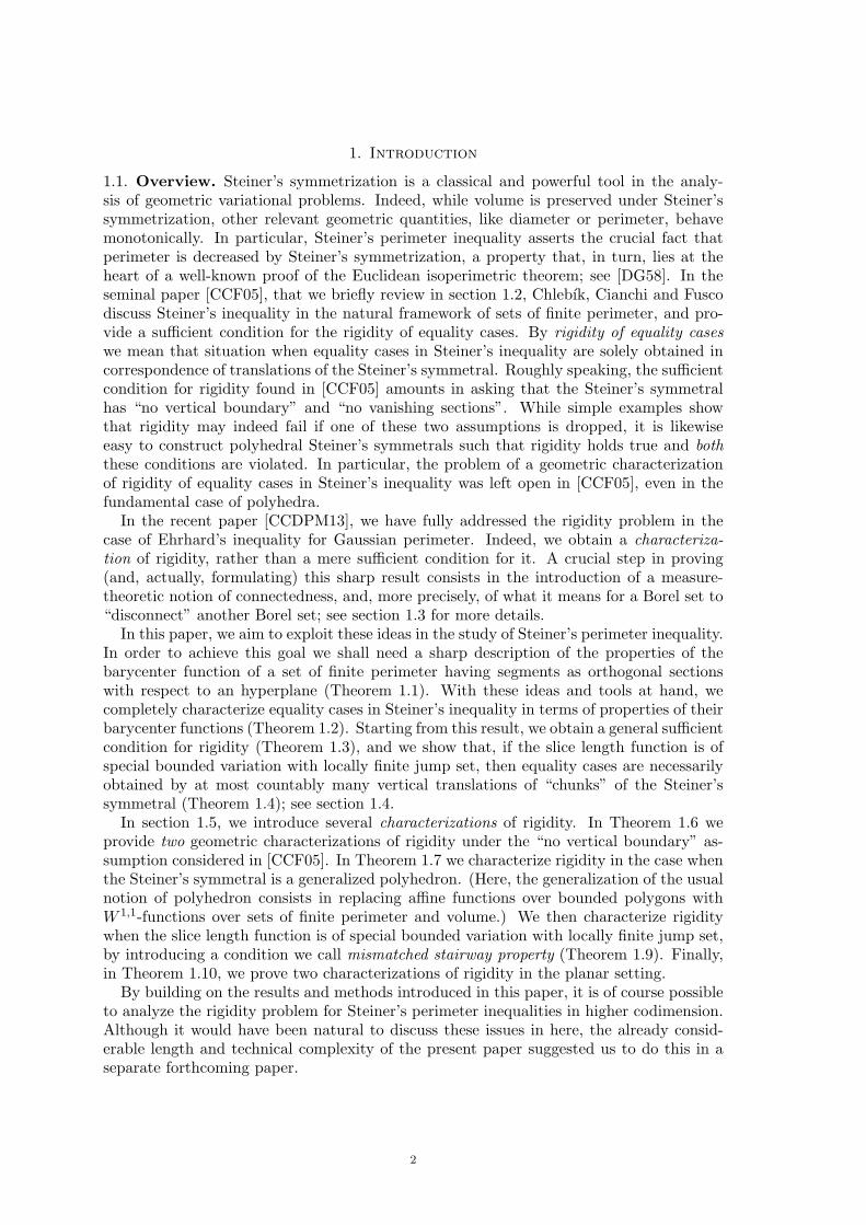
Figure 1.1. In case (a), ∂∗F [v] has vertical parts over Ω = (0, 1) and (1.6) does

not hold true; in case (b), ∂∗F [v] has no vertical parts over Ω = (0, 1), but (1.5)

fails (indeed, 0 = v∨(1/2) = v∧(1/2)), and, again, (1.6) does not hold true.

where, ∂∗E denotes the reduced boundary to E, while νE is the measure-theoretic outerunit normal of E; see section 2.2.

The second main result from [CCF05, Theorem 1.3] provides a sufficient condition forthe rigidity of equality cases in Steiner’s inequality over an open connected set. Noticeindeed that some assumptions are needed in order to expect rigidity; see Figure 1.1.

Theorem B ([CCF05]). If v ∈ BV (Rn−1), Ω ⊂ Rn−1 is an open connected set withHn−1(Ω) <∞, and

DsvxΩ = 0 , (1.4)

v∧ > 0 , Hn−2-a.e. on Ω , (1.5)

then for every E ∈ MΩ(v) we have

Hn((E∆(t en + F [v])

)∩ (Ω× R)

)= 0 , for some t ∈ R . (1.6)

Remark 1.1. Here, Dsv stands for the singular part of the distributional derivative Dv ofv, while v∧ and v∨ denote the approximate lower and upper limits of v (so that if v1 = v2a.e. on Rn−1, then v∨1 = v∨2 and v∧1 = v∧2 everywhere on Rn−1). We call [v] = v∨ − v∧

the jump of v, and define the approximate discontinuity set of v as Sv = v∨ > v∧ =[v] > 0, so that Sv is countably Hn−2-rectifiable, and there exists a Borel vector fieldνv : Sv → Sn−1 such that Dsv = νv [v]Hn−2xSv+Dcv, where Dcv stands for the Cantorianpart of Dv. These concepts are reviewed in sections 2.1 and 2.2.

Remark 1.2. Assumption (1.4) is clearly equivalent to asking that v ∈W 1,1(Ω) (so thatv∧ = v∨ Hn−2-a.e. on Ω), and, in turn, it is also equivalent to asking that ∂∗F [v] has novertical parts above Ω, that is, compare with (1.3),

Hn−1(x ∈ ∂∗F [v] ∩ (Ω× R) : qνF [v](x) = 0

)= 0 ; (1.7)

see [CCF05, Proposition 1.2] for a proof.

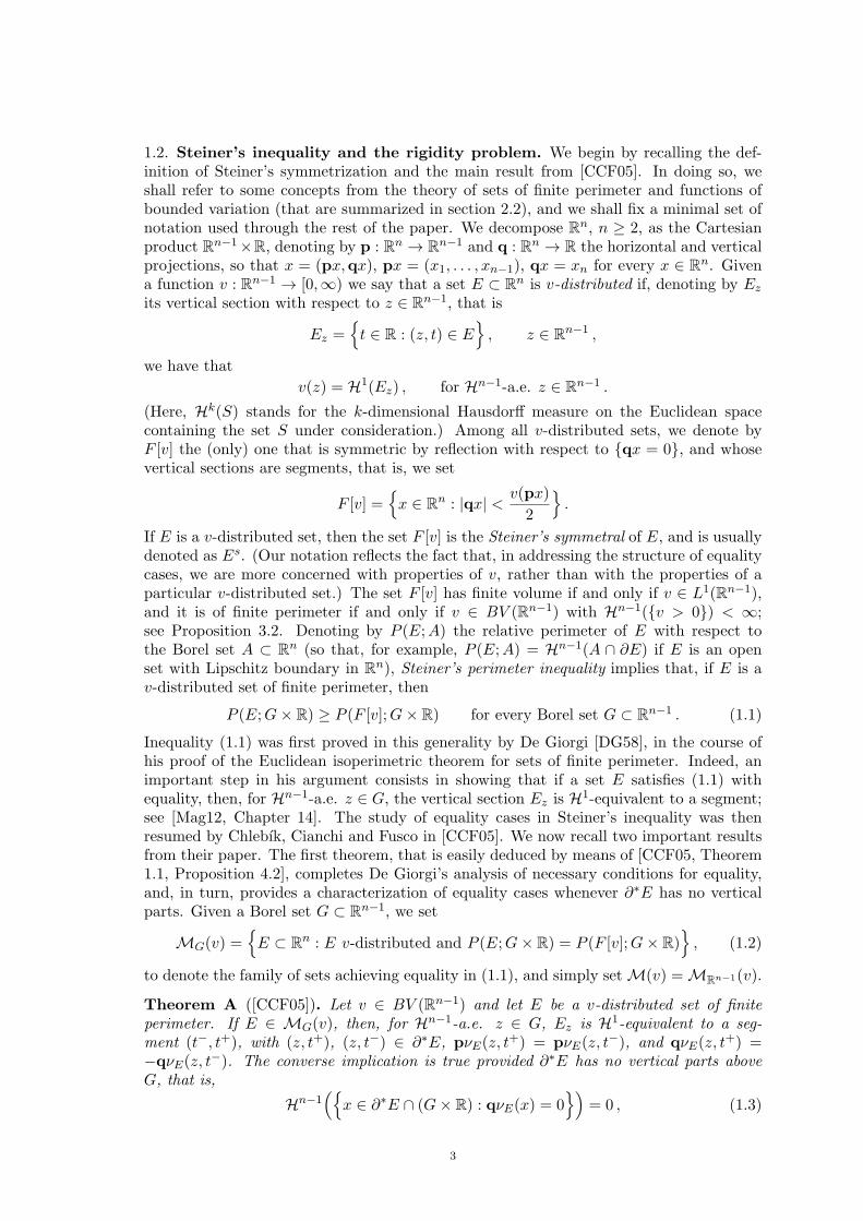
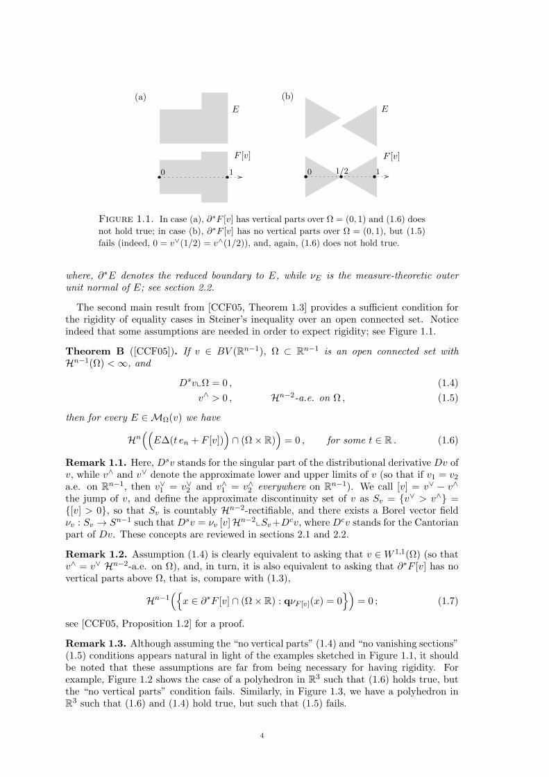
Remark 1.3. Although assuming the “no vertical parts” (1.4) and “no vanishing sections”(1.5) conditions appears natural in light of the examples sketched in Figure 1.1, it shouldbe noted that these assumptions are far from being necessary for having rigidity. Forexample, Figure 1.2 shows the case of a polyhedron in R3 such that (1.6) holds true, butthe “no vertical parts” condition fails. Similarly, in Figure 1.3, we have a polyhedron inR3 such that (1.6) and (1.4) hold true, but such that (1.5) fails.

4

[v] > 0

(0, 1)2

F [v]

Figure 1.2. A polyhedron in R3 such that the rigidity condition (1.6) holds

true (with Ω = (0, 1)2) but the “no vertical parts” condition fails.

v = 0

F [v](0, 1)2

Figure 1.3. A polyhedron in R3 such that the rigidity condition (1.6) and the

“no vertical parts” condition hold true (with Ω = (0, 1)2), but such that the “no

vanishing sections” condition fails.

1.3. Essential connectedness. The examples discussed in Figure 1.1 and Remark 1.3suggest that, in order to characterize rigidity of equality cases in Steiner’s inequality,one should first make precise, for example, in which sense a (n − 2)-dimensional set likeSv = v∧ < v∨ (contained into the projection of vertical boundaries) may disconnect the(n−1)-dimensional set v > 0 (that is, the projection of F [v]). In the study of rigidity ofequality cases for Ehrhard’s perimeter inequality, see [CCDPM13], we have satisfactorilyaddressed this kind of question by introducing the following definition.

Definition 1.1. LetK and G be Borel sets in Rm. One says thatK essentially disconnectsG if there exists a non-trivial Borel partition G+, G− of G modulo Hm such that

Hm−1((G(1) ∩ ∂eG+ ∩ ∂eG−

)\K

)= 0 ; (1.8)

conversely, one says that K does not essentially disconnect G if, for every non-trivial Borelpartition G+, G− of G modulo Hm,

Hm−1((G(1) ∩ ∂eG+ ∩ ∂eG−

)\K

)> 0 . (1.9)

Finally, G is essentially connected if ∅ does not essentially disconnect G.

Remark 1.4. By a non-trivial Borel partition G+, G− of G modulo Hm we mean that

Hm(G+ ∩G−) = 0 , Hm(G∆(G+ ∪G−)) = 0 , Hm(G+)Hm(G−) > 0 .

Moreover, ∂eG denotes the essential boundary of G, that is defined as

∂eG = Rm \ (G(0) ∪G(1)) ,

where G(0) and G(1) denote the sets of points of density 0 and 1 of G; see section 2.1.

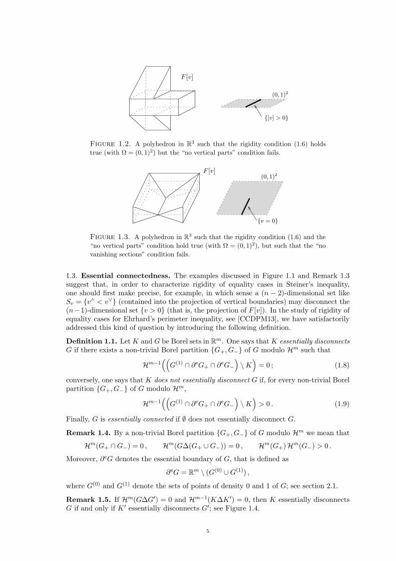
Remark 1.5. If Hm(G∆G′) = 0 and Hm−1(K∆K ′) = 0, then K essentially disconnectsG if and only if K ′ essentially disconnects G′; see Figure 1.4.

5

G+

K ′K

GG

G−

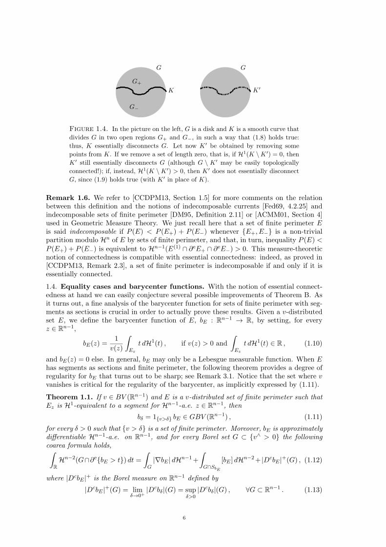
Figure 1.4. In the picture on the left, G is a disk and K is a smooth curve that

divides G in two open regions G+ and G−, in such a way that (1.8) holds true:

thus, K essentially disconnects G. Let now K ′ be obtained by removing some

points from K. If we remove a set of length zero, that is, if H1(K \K ′) = 0, then

K ′ still essentially disconnects G (although G \ K ′ may be easily topologically

connected!); if, instead, H1(K \K ′) > 0, then K ′ does not essentially disconnect

G, since (1.9) holds true (with K ′ in place of K).

Remark 1.6. We refer to [CCDPM13, Section 1.5] for more comments on the relationbetween this definition and the notions of indecomposable currents [Fed69, 4.2.25] andindecomposable sets of finite perimeter [DM95, Definition 2.11] or [ACMM01, Section 4]used in Geometric Measure Theory. We just recall here that a set of finite perimeter Eis said indecomposable if P (E) < P (E+) + P (E−) whenever E+, E− is a non-trivialpartition modulo Hn of E by sets of finite perimeter, and that, in turn, inequality P (E) <

P (E+) + P (E−) is equivalent to Hn−1(E(1) ∩ ∂eE+ ∩ ∂eE−) > 0. This measure-theoreticnotion of connectedness is compatible with essential connectedness: indeed, as proved in[CCDPM13, Remark 2.3], a set of finite perimeter is indecomposable if and only if it isessentially connected.

1.4. Equality cases and barycenter functions. With the notion of essential connect-edness at hand we can easily conjecture several possible improvements of Theorem B. Asit turns out, a fine analysis of the barycenter function for sets of finite perimeter with seg-ments as sections is crucial in order to actually prove these results. Given a v-distributedset E, we define the barycenter function of E, bE : Rn−1 → R, by setting, for everyz ∈ Rn−1,

bE(z) =1

v(z)

∫Ez

t dH1(t) , if v(z) > 0 and

∫Ez

t dH1(t) ∈ R , (1.10)

and bE(z) = 0 else. In general, bE may only be a Lebesgue measurable function. When Ehas segments as sections and finite perimeter, the following theorem provides a degree ofregularity for bE that turns out to be sharp; see Remark 3.1. Notice that the set where vvanishes is critical for the regularity of the barycenter, as implicitly expressed by (1.11).

Theorem 1.1. If v ∈ BV (Rn−1) and E is a v-distributed set of finite perimeter such thatEz is H1-equivalent to a segment for Hn−1-a.e. z ∈ Rn−1, then

bδ = 1v>δ bE ∈ GBV (Rn−1) , (1.11)

for every δ > 0 such that v > δ is a set of finite perimeter. Moreover, bE is approximatelydifferentiable Hn−1-a.e. on Rn−1, and for every Borel set G ⊂ v∧ > 0 the followingcoarea formula holds,∫

RHn−2(G∩∂ebE > t) dt =

∫G|∇bE | dHn−1+

∫G∩SbE

[bE ] dHn−2+ |DcbE |+(G) , (1.12)

where |DcbE |+ is the Borel measure on Rn−1 defined by

|DcbE |+(G) = limδ→0+

|Dcbδ|(G) = supδ>0

|Dcbδ|(G) , ∀G ⊂ Rn−1 . (1.13)

6

[v](z)2

v∧(z) > 0v∧(z) = 0

zz

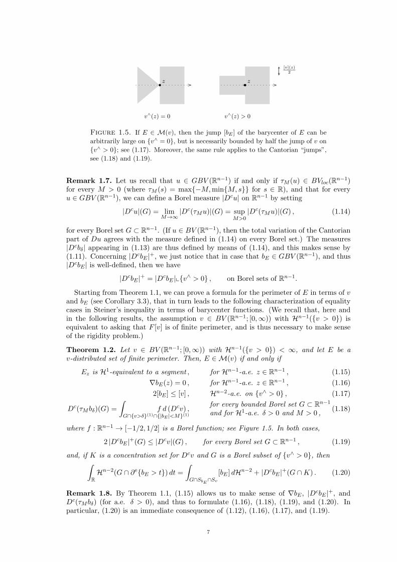
Figure 1.5. If E ∈ M(v), then the jump [bE ] of the barycenter of E can be

arbitrarily large on v∧ = 0, but is necessarily bounded by half the jump of v on

v∧ > 0; see (1.17). Moreover, the same rule applies to the Cantorian “jumps”,

see (1.18) and (1.19).

Remark 1.7. Let us recall that u ∈ GBV (Rn−1) if and only if τM (u) ∈ BVloc(Rn−1)for every M > 0 (where τM (s) = max−M,minM, s for s ∈ R), and that for everyu ∈ GBV (Rn−1), we can define a Borel measure |Dcu| on Rn−1 by setting

|Dcu|(G) = limM→∞

|Dc(τMu)|(G) = supM>0

|Dc(τMu)|(G) , (1.14)

for every Borel set G ⊂ Rn−1. (If u ∈ BV (Rn−1), then the total variation of the Cantorianpart of Du agrees with the measure defined in (1.14) on every Borel set.) The measures|Dcbδ| appearing in (1.13) are thus defined by means of (1.14), and this makes sense by(1.11). Concerning |DcbE |+, we just notice that in case that bE ∈ GBV (Rn−1), and thus|DcbE | is well-defined, then we have

|DcbE |+ = |DcbE |xv∧ > 0 , on Borel sets of Rn−1.

Starting from Theorem 1.1, we can prove a formula for the perimeter of E in terms of vand bE (see Corollary 3.3), that in turn leads to the following characterization of equalitycases in Steiner’s inequality in terms of barycenter functions. (We recall that, here andin the following results, the assumption v ∈ BV (Rn−1; [0,∞)) with Hn−1(v > 0) isequivalent to asking that F [v] is of finite perimeter, and is thus necessary to make senseof the rigidity problem.)

Theorem 1.2. Let v ∈ BV (Rn−1; [0,∞)) with Hn−1(v > 0) < ∞, and let E be av-distributed set of finite perimeter. Then, E ∈ M(v) if and only if

Ez is H1-equivalent to a segment , for Hn−1-a.e. z ∈ Rn−1 , (1.15)

∇bE(z) = 0 , for Hn−1-a.e. z ∈ Rn−1 , (1.16)

2[bE ] ≤ [v] , Hn−2-a.e. on v∧ > 0 , (1.17)

Dc(τMbδ)(G) =

∫G∩v>δ(1)∩|bE |<M(1)

f d (Dcv) ,for every bounded Borel set G ⊂ Rn−1

and for H1-a.e. δ > 0 and M > 0 ,(1.18)

where f : Rn−1 → [−1/2, 1/2] is a Borel function; see Figure 1.5. In both cases,

2 |DcbE |+(G) ≤ |Dcv|(G) , for every Borel set G ⊂ Rn−1 , (1.19)

and, if K is a concentration set for Dcv and G is a Borel subset of v∧ > 0, then∫RHn−2(G ∩ ∂ebE > t) dt =

∫G∩SbE

∩Sv

[bE ] dHn−2 + |DcbE |+(G ∩K) . (1.20)

Remark 1.8. By Theorem 1.1, (1.15) allows us to make sense of ∇bE , |DcbE |+, andDc(τMbδ) (for a.e. δ > 0), and thus to formulate (1.16), (1.18), (1.19), and (1.20). Inparticular, (1.20) is an immediate consequence of (1.12), (1.16), (1.17), and (1.19).

7

Theorem 1.2 is a powerful tool in the study of rigidity of equality cases. Indeed, rigidityamounts in asking that bE is constant on v > 0, a condition that, in turn, is equivalentto saying that there exists no subset I ⊂ R with H1(I) > 0 such that bE > t, bE ≤ tis a non-trivial Borel partition of v > 0 modulo Hn−1 for every t ∈ I. By combin-ing this information with the coarea formula (1.20) and with the definition of essentialconnectedness, we quite easily deduce the following sufficient condition for rigidity.

Theorem 1.3. If v ∈ BV (Rn−1; [0,∞)), Hn−1(v > 0) < ∞, and the Cantor part Dcvof Dv is concentrated on a Borel set K such that

v∧ = 0 ∪ Sv ∪K does not essentially disconnect v > 0 , (1.21)

then for every E ∈ M(v) there exists t ∈ R such that Hn(E∆(t en + F [v])) = 0.

Remark 1.9. The strength of Theorem 1.3 is that it provides a sufficient condition forrigidity without a priori structural assumption on F [v]. In particular, the theorem admitsfor non-trivial vertical boundaries and vanishing sections, that are excluded in TheoremB by (1.4) and (1.5). (In fact, as shown in Appendix A, Theorem B can be deduced fromTheorem 1.3.) We also notice that condition (1.21) is clearly not necessary for rigidity assoon as vertical boundaries are present; see Figure 1.2.

A natural question about equality cases of Steiner’s inequality that is left open by Theo-rem 1.2 is describing the situation when every E ∈ M(v) is obtained by at most countablymany vertical translations of parts of F [v]. In other words, we want to understand whento expect every E ∈ M(v) to satisfy

E =Hn

∪h∈I

(ch en + (F [v] ∩ (Gh × R))

)(1.22)

where I is at most countable, chh∈I ⊂ R, andGhh∈I is a Borel partition modulo Hn−1 of v > 0 .

The following theorem shows that this happens when v is of special bounded variationwith locally finite jump set. The notion of v-admissible partition of v > 0 used in thetheorem is introduced in Definition 1.4, see section 1.5.

Theorem 1.4. Let v ∈ SBV (Rn−1; [0,∞)) with Hn−1(v > 0) <∞, and

Sv ∩ v∧ > 0 is locally Hn−2-finite , (1.23)

and let E be a v-distributed set of finite perimeter. Then, E ∈ M(v) if and only if Esatisfies (1.22) for a v-admissible partition Ghh∈I of v > 0, and 2[bE ] ≤ [v] Hn−2-a.e.on v∧ > 0. Moreover, in both cases, |DcbE |+ = 0.

Remark 1.10. Let us recall that, by definition, v ∈ SBV (Rn−1) if v ∈ BV (Rn−1) andDcv = 0. The approximate discontinuity set Sv of a generic v ∈ SBV (Rn−1) is alwayscountably Hn−2-rectifiable, but it may fail to be locally Hn−2-finite. if v ∈ SBV (Rn−1)but (1.23) fails, then it may happen that (1.22) does not hold true for some E ∈ M(v);see Remark 1.12 below.

Remark 1.11. Condition (1.22) can be reformulated in terms of a property of the barycen-ter function. Indeed, (1.22) is equivalent to asking that

bE =∑h∈I

ch 1Gh, Hn−1-a.e. on Rn−1 , (1.24)

for I, chh∈I and Ghh∈I as in (1.22). It should be noted that, if no additional conditionsare assumed on the partition Ghh∈I , then (1.24) is not equivalent to saying that bEhas “countable range”. An example is obtained as follows. Let K be the middle-thirdCantor set in [0, 1], let Ghh∈N be the disjoint family of open intervals such that K =

8

[0, 1]\∪

h∈NGh, and let chh∈N ⊂ R be such that the Cantor function uK satisfies uK = chon Gh. In this way, uK =

∑h∈N ch 1Gh

on [0, 1] \ K, thus, H1-a.e. on [0, 1]. Of course,since uK is a non-constant, continuous, and increasing function, it does not have “countablerange” in any reasonable sense. At the same time, if we set v(z) = 1[0,1](z) dist(z,K) forz ∈ R, then v is a Lipschitz function on R (thus it satisfies all the assumptions in Theorem1.4) and the set

E =x ∈ R2 : uK(px)− v(px)

2< qx < uK(px) +

v(px)

2

,

is such that E ∈ M(v), as one can check by Corollary 3.3 and Corollary 3.4 in section 3.2.We also notice that, in this example, |DcbE |xv∧ = 0 = 0, while |DcbE |+ = 0.

Remark 1.12. We now provide the example introduced in Remark 1.10. Given qhh∈N =Q∩ [0, 1] and αhh∈N ∈ (0,∞) such that

∑h∈N αh <∞, we can define v ∈ SBV (R) such

that H1(v > 0) = 1 and Dv = Dsv = Djv, by setting

v(t) =∑

h∈N:qh<t≤1

αh =∑h∈N

αh 1(qh,1](t) , t ∈ R .

If we plug v1 = 0, v2 = v, and, say, λ = 0, in Proposition 1.5 below, then we obtain a setE ∈ M(v). At the same time, (1.24), thus (1.22), cannot hold true, as bE = v/2 H1-a.e.on R and v is strictly increasing on [0, 1]. (The requirement that the sets Gh in (1.24)are mutually disjoint modulo Hn−1 plays of course a crucial role in here.) Notice that, asexpected, Sv ∩ v∧ > 0 = Q ∩ [0, 1] is not locally H0-finite.

We close our analysis of equality cases with the following proposition, that shows ageneral way of producing equality cases in Steiner’s inequality that (potentially) do notsatisfy the basic structure condition (1.22).

Proposition 1.5. If v = v1 + v2 where v1, v2 ∈ BV (Rn−1; [0,∞)), Dv1 = Dav1, v2 is notconstant (modulo Hn−1) on v > 0, Dv2 = Dsv2, and 0 < Hn−1(v > 0) < ∞, thenrigidity fails for v. Indeed, if we set

E =x ∈ Rn : −λ v2(px)−

v1(px)

2≤ qx ≤ v1(px)

2+ (1− λ) v2(px)

, (1.25)

for λ ∈ [0, 1] \ 1/2, then E ∈ M(v) but Hn(E∆(t en + F [v])) > 0 for every t ∈ R.

1.5. Characterizations of rigidity. We now start to discuss the problem of character-izing rigidity of equality cases. We shall analyze this question under different geometricassumptions on the considered Steiner’s symmetral, and see how different structural as-sumptions lead to formulate different characterizations.

We begin our analysis by working under the assumption that no vertical boundaries arepresent where the slice length function v is essentially positive, that is, on v∧ > 0. Itturns out that, in this case, the sufficient condition (1.21) can be weakened to

v∧ = 0 does not essentially disconnect v > 0 , (1.26)

and that, in turn, this same condition is also necessary to rigidity. Moreover, an alternativecharacterization can obtained by merely requiring that F [v] is indecomposable.

Theorem 1.6. If v ∈ BV (Rn−1; [0,∞)) with Hn−1(v > 0) <∞, and

Dsvxv∧ > 0 = 0 , (1.27)

then the following three statements are equivalent:

(i) if E ∈ M(v) then Hn(E∆(t en + F [v])) = 0 for some t ∈ R;(ii) v∧ = 0 does not essentially disconnect v > 0;(iii) F [v] is indecomposable.

9

Remark 1.13. Notice that condition (1.27) does not prevent ∂∗F [v] to contain verticalparts, provided they are concentrated where the lower approximate limit of v vanishes.Indeed, it implies that Dcv = 0 (see step one in the proof of Theorem 1.6 in section 4.5),and that Sv is contained into v∧ = 0 modulo Hn−2.

Remark 1.14. We notice that the equivalence between conditions (ii) and (iii) is actuallytrue whenever v ∈ BV (Rn−1; [0,∞)) with Hn−1(v > 0) < ∞; in other words, (1.27)plays no role in proving this equivalence. This is proved in Theorem 4.2, section 4.4.

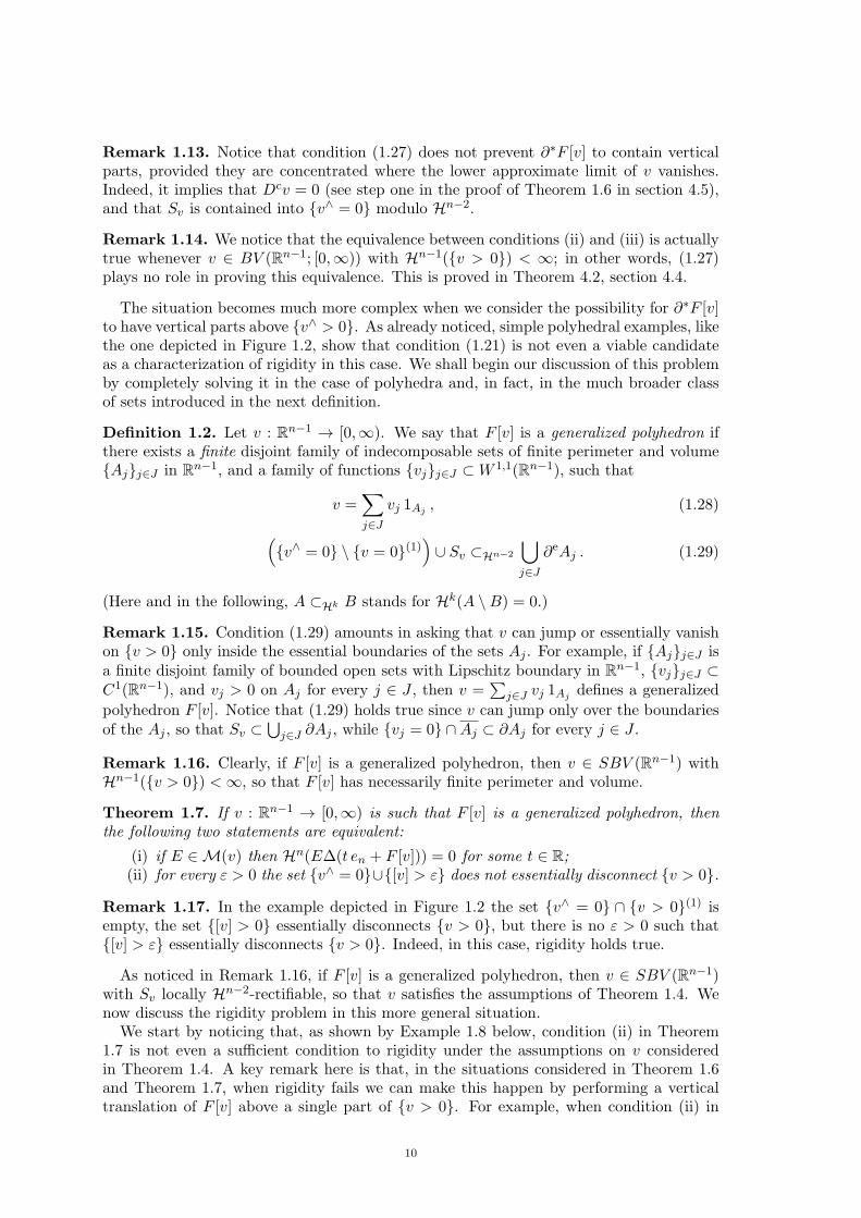
The situation becomes much more complex when we consider the possibility for ∂∗F [v]to have vertical parts above v∧ > 0. As already noticed, simple polyhedral examples, likethe one depicted in Figure 1.2, show that condition (1.21) is not even a viable candidateas a characterization of rigidity in this case. We shall begin our discussion of this problemby completely solving it in the case of polyhedra and, in fact, in the much broader classof sets introduced in the next definition.

Definition 1.2. Let v : Rn−1 → [0,∞). We say that F [v] is a generalized polyhedron ifthere exists a finite disjoint family of indecomposable sets of finite perimeter and volumeAjj∈J in Rn−1, and a family of functions vjj∈J ⊂W 1,1(Rn−1), such that

v =∑j∈J

vj 1Aj , (1.28)

(v∧ = 0 \ v = 0(1)

)∪ Sv ⊂Hn−2

∪j∈J

∂eAj . (1.29)

(Here and in the following, A ⊂Hk B stands for Hk(A \B) = 0.)

Remark 1.15. Condition (1.29) amounts in asking that v can jump or essentially vanishon v > 0 only inside the essential boundaries of the sets Aj . For example, if Ajj∈J isa finite disjoint family of bounded open sets with Lipschitz boundary in Rn−1, vjj∈J ⊂C1(Rn−1), and vj > 0 on Aj for every j ∈ J , then v =

∑j∈J vj 1Aj defines a generalized

polyhedron F [v]. Notice that (1.29) holds true since v can jump only over the boundariesof the Aj , so that Sv ⊂

∪j∈J ∂Aj , while vj = 0 ∩Aj ⊂ ∂Aj for every j ∈ J .

Remark 1.16. Clearly, if F [v] is a generalized polyhedron, then v ∈ SBV (Rn−1) withHn−1(v > 0) <∞, so that F [v] has necessarily finite perimeter and volume.

Theorem 1.7. If v : Rn−1 → [0,∞) is such that F [v] is a generalized polyhedron, thenthe following two statements are equivalent:

(i) if E ∈ M(v) then Hn(E∆(t en + F [v])) = 0 for some t ∈ R;(ii) for every ε > 0 the set v∧ = 0∪[v] > ε does not essentially disconnect v > 0.

Remark 1.17. In the example depicted in Figure 1.2 the set v∧ = 0 ∩ v > 0(1) isempty, the set [v] > 0 essentially disconnects v > 0, but there is no ε > 0 such that[v] > ε essentially disconnects v > 0. Indeed, in this case, rigidity holds true.

As noticed in Remark 1.16, if F [v] is a generalized polyhedron, then v ∈ SBV (Rn−1)with Sv locally Hn−2-rectifiable, so that v satisfies the assumptions of Theorem 1.4. Wenow discuss the rigidity problem in this more general situation.

We start by noticing that, as shown by Example 1.8 below, condition (ii) in Theorem1.7 is not even a sufficient condition to rigidity under the assumptions on v consideredin Theorem 1.4. A key remark here is that, in the situations considered in Theorem 1.6and Theorem 1.7, when rigidity fails we can make this happen by performing a verticaltranslation of F [v] above a single part of v > 0. For example, when condition (ii) in

10

32

32

12

11

12

18

38

58

78

98

118

138

158

14

34

74

54

Figure 1.6. The functions u2 and u4 in the construction of Example 1.8.

Theorem 1.7 fails, there exist ε > 0 and a non-trivial Borel partition G+, G− of v > 0modulo Hn−1 such that

v > 0(1) ∩ ∂eG+ ∩ ∂eG− ⊂Hn−2 v∧ = 0 ∪ [v] > ε .Correspondingly, as we shall prove later on, the v-distributed set E(t) defined as

E(t) =((t en + F [v]) ∩ (G+ × R)

)∪(F [v] ∩ (G− × R)

), t ∈ R ,

and obtained by a single vertical translation of F [v] above G+, satisfies P (E(t)) = P (F [v])whenever t ∈ (0, ε/2). (Moreover, when condition (1.26) fails, we have E(t) ∈ M(v) forevery t ∈ R.) However, there may be situations in which violating rigidity by a singlevertical translation of F [v] is impossible, but where this task can be accomplished bysimultaneously performing countably many independent vertical translations of F [v]. Anexample is obtained as follows.

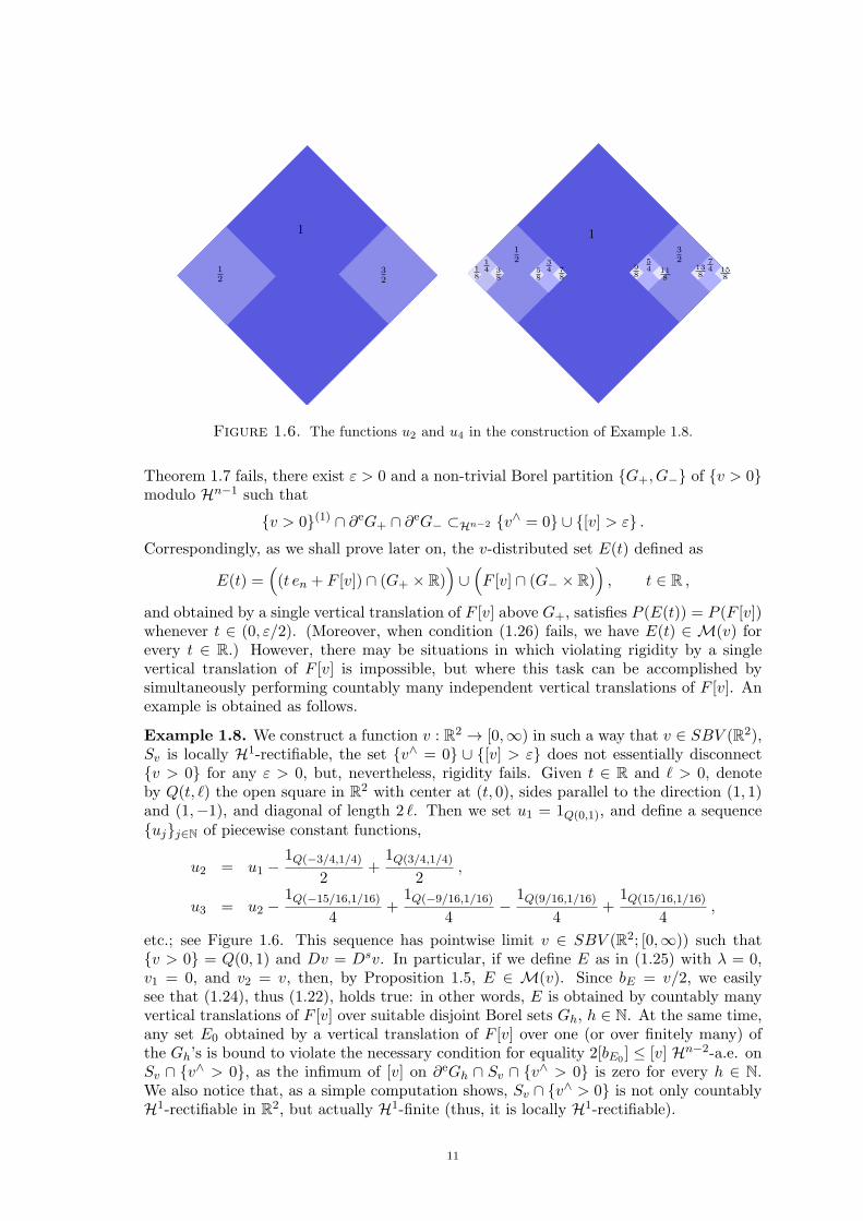
Example 1.8. We construct a function v : R2 → [0,∞) in such a way that v ∈ SBV (R2),Sv is locally H1-rectifiable, the set v∧ = 0 ∪ [v] > ε does not essentially disconnectv > 0 for any ε > 0, but, nevertheless, rigidity fails. Given t ∈ R and ℓ > 0, denoteby Q(t, ℓ) the open square in R2 with center at (t, 0), sides parallel to the direction (1, 1)and (1,−1), and diagonal of length 2 ℓ. Then we set u1 = 1Q(0,1), and define a sequenceujj∈N of piecewise constant functions,

u2 = u1 −1Q(−3/4,1/4)

2+

1Q(3/4,1/4)

2,

u3 = u2 −1Q(−15/16,1/16)

4+

1Q(−9/16,1/16)

4−

1Q(9/16,1/16)

4+

1Q(15/16,1/16)

4,

etc.; see Figure 1.6. This sequence has pointwise limit v ∈ SBV (R2; [0,∞)) such thatv > 0 = Q(0, 1) and Dv = Dsv. In particular, if we define E as in (1.25) with λ = 0,v1 = 0, and v2 = v, then, by Proposition 1.5, E ∈ M(v). Since bE = v/2, we easilysee that (1.24), thus (1.22), holds true: in other words, E is obtained by countably manyvertical translations of F [v] over suitable disjoint Borel sets Gh, h ∈ N. At the same time,any set E0 obtained by a vertical translation of F [v] over one (or over finitely many) ofthe Gh’s is bound to violate the necessary condition for equality 2[bE0 ] ≤ [v] Hn−2-a.e. onSv ∩ v∧ > 0, as the infimum of [v] on ∂eGh ∩ Sv ∩ v∧ > 0 is zero for every h ∈ N.We also notice that, as a simple computation shows, Sv ∩ v∧ > 0 is not only countablyH1-rectifiable in R2, but actually H1-finite (thus, it is locally H1-rectifiable).

11

All the above considerations finally suggest to introduce the following condition, that,in turn, characterizes rigidity under the assumptions on v considered in Theorem 1.4. Webegin by recalling the definition of Caccioppoli partition.

Definition 1.3. Let G ⊂ Rn−1 be a set of finite perimeter, and let Ghh∈I be an atmost countable Borel partition of G modulo Hn−1. (That is, I is a finite or countable setwith # I ≥ 2, G =Hn−1

∪h∈I Gh, Hn−1(Gh) > 0 for every h ∈ I and Hn−1(Gh ∩Gk) = 0

for every h, k ∈ I, h = k.) We say that Ghh∈I is a Caccioppoli partition of G, if∑h∈I P (Gh) <∞.

Remark 1.18. WhenG is an open set and Ghh∈I is an at most countable Borel partitionof G modulo Hn−1, then, according to [AFP00, Definition 4.16], Ghh∈I is a Caccioppolipartition of G if

∑h∈I P (Gh;G) < ∞. Of course, if we assume in addition that G is

of finite perimeter, then∑

h∈I P (Gh;G) < ∞ is equivalent to∑

h∈I P (Gh) < ∞. ThusDefinition 1.3 and [AFP00, Definition 4.16] agree in their common domain of applicability(that is, on open sets of finite perimeter).

Definition 1.4. Let v ∈ BV (Rn−1; [0,∞)), and let Ghh∈I be an at most countableBorel partition of v > 0. We say that Ghh∈I is a v-admissible partition of v > 0, ifGh ∩ BR ∩ v > δh∈I is a Caccioppoli partition of v > δ ∩ BR, for every δ > 0 suchthat v > δ is of finite perimeter and for every R > 0.

Definition 1.5. One says that v ∈ BV (Rn−1; [0,∞)) satisfies the mismatched stairwayproperty if the following holds: If Ghh∈I is a v-admissible partition of v > 0 and ifchh∈I ⊂ R is a sequence with ch = ck whenever h = k, then there exist h0, k0 ∈ I withh0 = k0, and a Borel set Σ with

Σ ⊂ ∂eGh0 ∩ ∂eGk0 ∩ v∧ > 0 , Hn−2(Σ) > 0 , (1.30)

such that

[v](z) < 2|ch0 − ck0 | , ∀z ∈ Σ . (1.31)

Remark 1.19. The terminology adopted here would like to suggest the following idea.One considers a v-admissible partition Ghh∈I of v > 0 such that v > 0(1)∩

∪h∈I ∂

eGh

is contained into v∧ = 0∪Sv. Next, one modifies F [v] by performing vertical translationsch above each Gh, thus constructing a new set E having a “stairway-like” barycenter. Thisnew set will have the same perimeter of F [v], and thus will violate rigidity if # I ≥ 2,provided all the steps of the stairway match the jumps of v, in the sense that 2[bE ] =2|ch − ck| ≤ [v] on each ∂eGh ∩ ∂eGk ∩ v∧ > 0. Thus, when all equality cases arestairway-like, we expect rigidity to be equivalent to asking that every such stairway hasat least one step that is mismatched with respect to [v].

Remark 1.20. If v ∈ BV (Rn−1; [0,∞)) has the mismatched stairway property, then, forevery ε > 0, v∧ = 0 ∪ [v] > ε does not essentially disconnect v > 0. In particular,v∧ = 0 does not essentially disconnect v > 0, v > 0 is essentially connected, andalthough it may still happen that v∧ = 0 ∪ Sv essentially disconnects v > 0, in thiscase one has

Hn−2-ess infSv∩v∧>0

[v] = 0 .

We prove the claim arguing by contradiction. If v∧ = 0∪[v] > ε essentially disconnectsv > 0, then there exist ε > 0 and a non-trivial Borel partition G+, G− of v > 0modulo Hn−1 such that v > 0(1)∩∂eG+∩∂eG− ⊂Hn−2 v∧ = 0∪[v] > ε. Since (2.9)below implies v∧ > 0 ⊂ v > 0(1), then we have

v∧ > 0 ∩ ∂eG+ ∩ ∂eG− ⊂Hn−2 [v] > ε , (1.32)

12

so that, for every δ > 0,

v > δ(1) ∩ ∂eG+ = v > δ(1) ∩ ∂eG+ ∩ ∂eG− ⊂Hn−2 [v] > ε . (1.33)

If we set G± δ = G± ∩ v > δ, then ∂eG± δ ⊂ ∂ev > δ ∪ (v > δ(1) ∩ ∂eG±), and,by (1.33), ∂eG± δ ⊂Hn−2 ∂ev > δ ∪ [v] > ε. Since [v] ∈ L1(Hn−2xSv), we findHn−2([v] > t) <∞ for every t > 0, and, in particular

P (G+ δ) + P (G− δ) ≤ 2P (v > δ) + 2Hn−2([v] > ε) <∞ ,

whenever v > δ is of finite perimeter. This shows that G+, G− is a v-admissiblepartition. If we now set I = +,−, c+ = ε/2, and c− = 0, then I, Ghh∈I , and chh∈Iare admissible in the mismatched stairway property. By the mismatched stairway property,there exists a Borel set Σ ⊂ v∧ > 0 ∩ ∂eG+ ∩ ∂eG− such that [v] < 2|c+ − c−| = ε on Σand Hn−2(Σ) > 0, a contradiction to (1.32).

It turns out that if v is a SBV -function with locally finite jump set, then rigidity ischaracterized by the mismatched stairway property.

Theorem 1.9. If v ∈ SBV (Rn−1; [0,∞)), Hn−1(v > 0) < ∞, and Sv ∩ v∧ > 0 islocally Hn−2-finite, then the following two statements are equivalent:

(i) if E ∈ M(v), then Hn(E∆(t en + F [v])) = 0 for some t ∈ R;(ii) v has the mismatched stairway property.

Remark 1.21. Is it important to observe that, in order to characterize rigidity, only v-admissible partitions of v > 0 have to be considered in the definition of mismatchedstairway property. Indeed, let n = 2 and set v = 1(0,1) ∈ SBV (R; [0,∞)), so that rigidityholds true for v. Let now Ghh∈N be the family of open intervals used to define themiddle-third Cantor set K, so that K = [0, 1] \

∪h∈NGh. Notice that Ghh∈N is a

non-trivial countable Borel partition of v > 0 = (0, 1) modulo H1. However, since∂eGh ∩ ∂eGk = ∅ whenever h = k, it is not possible to find a set Σ satisfying (1.30)whatever the choice of chh∈N we make. In particular, if we would not restrict thepartitions in Definition 1.5 to v-admissible partitions, then this particular v (satisfyingrigidity) would not have the mismatched stairway property. Notice of course that, in thisexample,

∑h∈N P (Gh ∩ v > δ ∩BR) = ∞ for every δ,R > 0.

The question for a geometric characterization of rigidity when v ∈ BV is thus leftopen. The considerable complexity of the mismatched stairway property may be seen asa negative indication about the tractability of this problem. In the planar case, due tothe trivial topology of the real line, these difficulties can be overcome, and we obtain thefollowing complete result.

Theorem 1.10. If v ∈ BV (R; [0,∞)) and H1(v > 0) <∞, then, equivalently,

(i) if E ∈ M(v), then H2(E∆(t e2 + F [v])) = 0 for some t ∈ R;(ii) v > 0 is H1-equivalent to a bounded open interval (a, b), v ∈ W 1,1(a, b), and

v∧ > 0 on (a, b);(iii) F [v] is an indecomposable set that has no vertical boundary above v∧ > 0, i.e.

H1(x ∈ ∂∗F [v] : qνF [v](x) = 0 , v∧(px) > 0

)= 0 . (1.34)

We close this introduction by mentioning that the extension of our results to the caseof the localized Steiner’s inequality is discussed in appendix A. In particular, we shallexplain how to derive Theorem B from Theorem 1.3 via an approximation argument.

Acknowledgement : This work was carried out while FC, MC, and GDP were visiting theUniversity of Texas at Austin. The work of FC was partially supported by the UT Austin-Portugal partnership through the FCT post-doctoral fellowship SFRH/BPD/51349/2011.The work of GDP was partially supported by ERC under FP7, Advanced Grant n. 246923.

13

The work of FM was partially supported by ERC under FP7, Starting Grant n. 258685 andAdvanced Grant n. 226234, by the Institute for Computational Engineering and Sciencesand by the Mathematics Department of the University of Texas at Austin during his visitto these institutions, and by NSF Grant DMS-1265910.

2. Notions from Geometric Measure Theory

We gather here some notions from Geometric Measure Theory needed in the sequel,referring to [AFP00, Mag12] for further details. We start by reviewing our general notationin Rn. We denote by B(x, r) the open Euclidean ball of radius r > 0 and center x ∈ Rn.Given x ∈ Rn and ν ∈ Sn−1 we denote by H+

x,ν and H−x,ν the complementary half-spaces

H+x,ν =

y ∈ Rn : (y − x) · ν ≥ 0

, (2.1)

H−x,ν =

y ∈ Rn : (y − x) · ν ≤ 0

.

Finally, we decompose Rn as the product Rn−1 × R, and denote by p : Rn → Rn−1 andq : Rn → R the corresponding horizontal and vertical projections, so that

x = (px,qx) = (x′, xn) , x′ = (x1, . . . , xn−1) , ∀x ∈ Rn ,

and define the vertical cylinder of center x ∈ Rn and radius r > 0, and the (n − 1)-dimensional ball in Rn−1 of center z ∈ Rn−1 and radius r > 0, by setting, respectively,

Cx,r =y ∈ Rn : |px− py| < r , |qx− qy| < r

,

Dz,r =w ∈ Rn−1 : |w − z| < r

.

In this way, Cx,r = Dpx,r × (qx − r,qx + r). We shall use the following two notionsof convergence for Lebesgue measurable subsets of Rn. Given Lebesgue measurable setsEhh∈N and E in Rn, we shall say that Eh locally converge to E, and write

Ehloc→ E , as h→ ∞ ,

provided Hn((Eh∆E)∩K) → 0 as h→ ∞ for every compact set K ⊂ Rn; we say that Eh

converge to E as h→ ∞, and write Eh → E, provided Hn(Eh∆E) → 0 as h→ ∞.

2.1. Density points and approximate limits. If E is a Lebesgue measurable set inRn and x ∈ Rn, then we define the upper and lower n-dimensional densities of E at x as

θ∗(E, x) = lim supr→0+

Hn(E ∩B(x, r))

ωn rn, θ∗(E, x) = lim inf

r→0+

Hn(E ∩B(x, r))

ωn rn,

respectively. In this way we define two Borel functions on Rn, that agree a.e. on Rn. Inparticular, the n-dimensional density of E at x

θ(E, x) = limr→0+

Hn(E ∩B(x, r))

ωn rn,

is defined for a.e. x ∈ Rn, and θ(E, ·) is a Borel function on Rn (up to extending itby a constant value on the Hn-negligible set θ∗(E, ·) > θ∗(E, ·)). Correspondingly, fort ∈ [0, 1], we define

E(t) =x ∈ Rn : θ(E, x) = t

. (2.2)

By the Lebesgue differentiation theorem, E(0), E(1) is a partition of Rn up to a Hn-negligible set. It is useful to keep in mind that

x ∈ E(1) if and only if Ex,rloc→ Rn as r → 0+ ,

x ∈ E(0) if and only if Ex,rloc→ ∅ as r → 0+ ,

14

where Ex,r denotes the blow-up of E at x at scale r, defined as

Ex,r =E − x

r=

y − x

r: y ∈ E

, x ∈ Rn , r > 0 .

The set ∂eE = Rn \ (E(0) ∪ E(1)) is called the essential boundary of E. Thus, in general,we only have Hn(∂eE) = 0, but we do not know ∂eE to be “(n− 1)-dimensional” in anysense. Strictly related to the notion of density is that of approximate upper and lowerlimits of a measurable function. Given a Lebesgue measurable function f : Rn → R wedefine the (weak) approximate upper and lower limits of f at x ∈ Rn as

f∨(x) = inft ∈ R : θ(f > t, x) = 0

= inf

t ∈ R : θ(f < t, x) = 1

,

f∧(x) = supt ∈ R : θ(f < t, x) = 0

= sup

t ∈ R : θ(f > t, x) = 1

.

As it turns out, f∨ and f∧ are Borel functions with values on R ∪ ±∞ defined at everypoint x of Rn, and they do not depend on the Lebesgue representative chosen for thefunction f . Moreover, for Hn-a.e. x ∈ Rn, we have that f∨(x) = f∧(x) ∈ R ∪ ±∞, sothat the approximate discontinuity set of f , Sf = f∧ < f∨, satisfies Hn(Sf ) = 0. Onnoticing that, even if f∧ and f∨ may take infinite values on Sf , the difference f

∨(x)−f∧(x)is always well defined in R ∪ ±∞ for x ∈ Sf , we define the approximate jump of f asthe Borel function [f ] : Rn → [0,∞] defined by

[f ](x) =

f∨(x)− f∧(x) , if x ∈ Sf ,0 , if x ∈ Rn \ Sf .

so that Sf = [f ] > 0. Finally, the approximate average of f is the Borel function

f : Rn → R ∪ ±∞ defined as

f(x) =

f∨(x)+f∧(x)

2 , if x ∈ Rn \ f∧ = −∞ , f∨ = +∞ ,0 , if x ∈ f∧ = −∞ , f∨ = +∞ .

(2.3)

The motivation behind definition (2.3) is that (in step two of the proof of Theorem 3.1)we want the limit relation

f(x) = limM→∞

τM (f)(x) = limM→∞

τM (f∨) + τM (f∧)

2, ∀x ∈ Rn , (2.4)

to hold true for every Lebesgue measurable function f : Rn → R, where here and in therest of the paper we set

τM (s) = max−M,minM, s , s ∈ R ∪ ±∞ . (2.5)

The validity of (2.4) is easily checked by noticing that

τM (f)∧ = τM (f∧) , τM (f)∨ = τM (f∨) , τM (f)(x) =τM (f∨) + τM (f∧)

2. (2.6)

With these definitions at hand, we notice the validity of the following properties, whichfollow easily from the above definitions, and hold true for every Lebesgue measurablef : Rn → R and for every t ∈ R:

|f |∨ < t = −t < f∧ ∩ f∨ < t , (2.7)

f∨ < t ⊂ f < t(1) ⊂ f∨ ≤ t , (2.8)

f∧ > t ⊂ f > t(1) ⊂ f∧ ≥ t . (2.9)

(Note that all the inclusions may be strict, that we also have f < t(1) = f∨ < t(1), andthat all the other analogous relations hold true.) Moreover, if f, g : Rn → R are Lebesguemeasurable functions and f = g Hn-a.e. on a Borel set E, then

f∨(x) = g∨(x) , f∧(x) = g∧(x) , [f ](x) = [g](x) , ∀x ∈ E(1) . (2.10)

15

If f : Rn → R and A ⊂ Rn are Lebesgue measurable, and x ∈ Rn is such that θ∗(A, x) > 0,then we say that t ∈ R ∪ ±∞ is the approximate limit of f at x with respect to A, andwrite t = ap lim(f,A, x), if

θ(|f − t| > ε ∩A;x

)= 0 , ∀ε > 0 , (t ∈ R) ,

θ(f < M ∩A;x

)= 0 , ∀M > 0 , (t = +∞) ,

θ(f > −M ∩A;x

)= 0 , ∀M > 0 , (t = −∞) .

We say that x ∈ Sf is a jump point of f if there exists ν ∈ Sn−1 such that

f∨(x) = ap lim(f,H+x,ν , x) , f∧(x) = ap lim(f,H−

x,ν , x) .

If this is the case we set ν = νf (x), the approximate jump direction of f at x. We denoteby Jf the set of approximate jump points of f , so that Jf ⊂ Sf ; moreover, νf : Jf → Sn−1

is a Borel function. It will be particularly useful to keep in mind the following proposition;see [CCDPM13, Proposition 2.2] for a proof.

Proposition 2.1. We have that x ∈ Jf if and only if for every τ ∈ (f∧(x), f∨(x)),

f > τx,rloc→ H+

0,ν , f < τx,rloc→ H−

0,ν , as r → 0+ . (2.11)

Finally, if f : Rn → R is Lebesgue measurable, then we say f is approximately differen-tiable at x ∈ Sc

f provided f∧(x) = f∨(x) ∈ R and there exists ξ ∈ Rn such that

ap lim(g,Rn, x) = 0 ,

where g(y) = (f(y)− f(x)−ξ · (y−x))/|y−x| for y ∈ Rn \x. If this is the case, then ξ isuniquely determined, we set ξ = ∇f(x), and call ∇f(x) the approximate differential of f atx. The localization property (2.10) holds true also for approximate differentials: precisely,if f, g : Rn → R are Lebesgue measurable functions, f = g Hn-a.e. on a Borel set E,and f is approximately differentiable Hn-a.e. on E, then g is approximately differentiableHn-a.e. on E too, with

∇f(x) = ∇g(x) , for Hn-a.e. x ∈ E . (2.12)

2.2. Rectifiable sets and functions of bounded variation. Let 1 ≤ k ≤ n, k ∈ N. ABorel setM ⊂ Rn is countably Hk-rectifiable if there exist Lipschitz functions fh : Rk → Rn

(h ∈ N) such that M ⊂Hk

∪h∈N fh(Rk). We further say that M is locally Hk-rectifiable

if Hk(M ∩K) < ∞ for every compact set K ⊂ Rn, or, equivalently, if HkxM is a Radonmeasure on Rn. Hence, for a locally Hk-rectifiable set M in Rn the following definitionis well-posed: we say that M has a k-dimensional subspace L of Rn as its approximatetangent plane at x ∈ Rn, L = TxM , if Hkx(M − x)/r HkxL as r → 0+ weakly-starin the sense of Radon measures. It turns out that TxM exists and is uniquely defined atHk-a.e. x ∈M . Moreover, given two locally Hk-rectifiable setsM1 andM2 in Rn, we haveTxM1 = TxM2 for Hk-a.e. x ∈M1 ∩M2.

A Lebesgue measurable set E ⊂ Rn is said of locally finite perimeter in Rn if there existsa Rn-valued Radon measure µE , called the Gauss–Green measure of E, such that∫

E∇φ(x) dx =

∫Rn

φ(x) dµE(x) , ∀φ ∈ C1c (Rn) .

The relative perimeter of E in A ⊂ Rn is then defined by setting P (E;A) = |µE |(A),while P (E) = P (E;Rn) is the perimeter of E. The reduced boundary of E is the set ∂∗Eof those x ∈ Rn such that

νE(x) = limr→0+

µE(B(x, r))

|µE |(B(x, r))exists and belongs to Sn−1 .

16

The Borel function νE : ∂∗E → Sn−1 is called the measure-theoretic outer unit normal toE. It turns out that ∂∗E is a locally Hn−1-rectifiable set in Rn [Mag12, Corollary 16.1],that µE = νE Hn−1x∂∗E, and that∫

E∇φ(x) dx =

∫∂∗E

φ(x) νE(x) dHn−1(x) , ∀φ ∈ C1c (Rn) .

In particular, P (E;A) = Hn−1(A∩ ∂∗E) for every Borel set A ⊂ Rn. We say that x ∈ Rn

is a jump point of E, if there exists ν ∈ Sn−1 such that

Ex,rloc→ H+

0,ν , as r → 0+ , (2.13)

and we denote by ∂JE the set of jump points of E. Notice that we always have ∂JE ⊂E(1/2) ⊂ ∂eE. In fact, if E is a set of locally finite perimeter and x ∈ ∂∗E, then (2.13)holds true with ν = −νE(x), so that ∂∗E ⊂ ∂JE. Summarizing, if E is a set of locallyfinite perimeter, we have

∂∗E ⊂ ∂JE ⊂ E1/2 ⊂ ∂eE , (2.14)

and, moreover, by Federer’s theorem [AFP00, Theorem 3.61], [Mag12, Theorem 16.2],

Hn−1(∂eE \ ∂∗E) = 0 ,

so that ∂eE is locally Hn−1-rectifiable in Rn. We shall need at several occasions to usethe following very fine criterion for finite perimeter, known as Federer’s criterion [Fed69,4.5.11] (see also [EG92, Theorem 1, section 5.11]): if E is a Lebesgue measurable set inRn such that ∂eE is locally Hn−1-finite, then E is a set of locally finite perimeter.

Given a Lebesgue measurable function f : Rn → R and an open set Ω ⊂ Rn we definethe total variation of f in Ω as

|Df |(Ω) = sup∫

Ωf(x) div T (x) dx : T ∈ C1

c (Ω;Rn) , |T | ≤ 1.

We say that f ∈ BV (Ω) if |Df |(Ω) < ∞ and f ∈ L1(Ω), and that f ∈ BVloc(Ω) iff ∈ BV (Ω′) for every open set Ω′ compactly contained in Ω. If f ∈ BVloc(Rn) then thedistributional derivative Df of f is an Rn-valued Radon measure. Notice in particularthat E is a set of locally finite perimeter if and only if 1E ∈ BVloc(Rn), and that in thiscase µE = −D1E . Sets of finite perimeter and functions of bounded variation are relatedby the fact that, if f ∈ BVloc(Rn), then, for a.e. t ∈ R, f > t is a set of finite perimeter,and the coarea formula, ∫

RP (f > t;G) dt = |Df |(G) , (2.15)

holds true (as an identity in [0,∞]) for every Borel set G ⊂ Rn. If f ∈ BVloc(Rn),then the Radon–Nykodim decomposition of Df with respect to Hn is denoted by Df =Daf+Dsf , where Dsf and Hn are mutually singular, and where Daf ≪ Hn. The densityof Daf with respect to Hn is by convention denoted as ∇f , so that ∇ f ∈ L1(Ω;Rn) withDaf = ∇f dHn. Moreover, for a.e. x ∈ Rn, ∇f(x) is the approximate differential of fat x. If f ∈ BVloc(Rn), then Sf is countably Hn−1-rectifiable, with Hn−1(Sf \ Jf ) = 0,[f ] ∈ L1

loc(Hn−1xJf ), and the Rn-valued Radon measure Djf defined as

Djf = [f ] νf dHn−1xJf ,is called the jump part of Df . Since Daf and Djf are mutually singular, by settingDcf = Dsf − Djf we come to the canonical decomposition of Df into the sum Daf +Djf + Dcf . The Rn-valued Radon measure Dcf is called the Cantorian part of Df . Ithas the distinctive property that |Dcf |(M) = 0 if M is σ-finite with respect to Hn−1. Weshall often need to use (in combination with (2.10) and (2.12)) the following localizationproperty of Cantorian derivatives.

17

Lemma 2.2. If v ∈ BV (Rn), then |Dcv|(v∧ = 0) = 0. In particular, if f, g ∈ BV (Rn)

and f = g Hn-a.e. on a Borel set E, then DcfxE(1) = DcgxE(1).

Proof. Step one: Let v ∈ BV (Rn), and let K ⊂ Scv be a concentration set for Dcv that is

Hn-negligible. By the coarea formula,

|Dcv|(v∧ = 0) = |Dcv|(K ∩ v∧ = 0) = |Dv|(K ∩ v∧ = 0)

=

∫RHn−2(K ∩ v∧ = 0 ∩ ∂∗v > t) dt

(by v∧ = v∨ on Scv) =

∫RHn−2(K ∩ v = 0 ∩ ∂∗v > t) dt = 0 .

where in the last identity we have noticed that v = 0 ∩ ∂∗v > t ∩ Scv = ∅ if t = 0.

Step two: Let f, g ∈ BV (Rn) with f = g Hn-a.e. on a Borel set E. Let v = f − g so that

v ∈ BV (Rn). Since v = 0 on E we easily see that E(1) ⊂ v = 0. Thus |Dcv|(E(1)) = 0by step one. Lemma 2.3. If f, g ∈ BV (Rn), E is a set of finite perimeter, and f = 1E g, then

∇f = 1E ∇g , Hn-a.e. on Rn , (2.16)

Dcf = DcgxE(1) , (2.17)

Sf ∩ E(1) = Sg ∩ E(1) . (2.18)

Proof. Since f = g on E by (2.12) we find that ∇f = ∇g Hn-a.e. on E; since f = 0on Rn \ E, again by (2.12) we find that ∇f = 0 Hn-a.e. on Rn \ E; this proves (2.16).For the same reasons, but this time exploiting Lemma 2.2 in place of (2.12), we see that

DcfxE(1) = DcgxE(1) and that Dcfx(Rn \ E)(1) = DcfxE(0) = 0; since ∂eE is locallyHn−2-rectifiable, and thus |Dcf |-negligible, we come to prove (2.17). Finally, (2.18) is animmediate consequence of (2.10).

Given a Lebesgue measurable function f : Rn → R we say that f is a function ofgeneralized bounded variation on Rn, f ∈ GBV (Rn), if ψ f ∈ BVloc(Rn) for everyψ ∈ C1(R) with ψ′ ∈ C0

c (R), or, equivalently, if τM (f) ∈ BVloc(Rn) for every M > 0,where τM was defined in (2.5). Notice that, if f ∈ GBV (Rn), then we do not even askthat f ∈ L1

loc(Rn), so that the distributional derivative Df of f may even fail to bedefined. Nevertheless, the structure theory of BV -functions holds true for GBV -functionstoo. Indeed, if f ∈ GBV (Rn), then, see [AFP00, Theorem 4.34], f > t is a set of finiteperimeter for a.e. t ∈ R, f is approximately differentiable Hn-a.e. on Rn, Sf is countablyHn−1-rectifiable and Hn−1-equivalent to Jf , and the coarea formula (2.15) takes the form∫

RP (f > t;G) dt =

∫G|∇f | dHn +

∫G∩Sf

[f ] dHn−1 + |Dcf |(G) , (2.19)

for every Borel set G ⊂ Rn, where |Dcf | denotes the Borel measure on Rn defined as theleast upper bound of the Radon measures |Dc(τM (f))|; and, in fact,

|Dcf |(G) = limM→∞

|Dc(τM (f))|(G) = supM>0

|Dc(τM (f))|(G) , (2.20)

whenever G is a Borel set in Rn; see [AFP00, Definition 4.33].

3. Characterization of equality cases and barycenter functions

We now prove the results presented in section 1.4. In section 3.1, Theorem 3.1, weobtain a formula for the perimeter of a set whose sections are segments, which is thenapplied in section 3.2 to study barycenter functions of such sets, and prove Theorem 1.1.Sections 3.3 and 3.4 contain the proof of Theorem 1.2 concerning the characterization ofequality cases in terms of barycenter functions, while Theorem 1.4 is proved in section 3.5.

18

3.1. Sets with segments as sections. Given u : Rn−1 → R ∪ ±∞, let us denote byΣu = x ∈ Rn : qx > u(px) and Σu = x ∈ Rn : qx < u(px), respectively, the epigraphand the subgraph of u. As proved in [CCDPM13, Proposition 3.1], Σu is a set of locallyfinite perimeter if and only if τM (u) ∈ BVloc(Rn−1) for every M > 0. (Note that this doesnot mean that u ∈ GBV (Rn−1), as here u takes values in R∪±∞.) Moreover, it is wellknown that if u ∈ BVloc(Rn−1), then, for every Borel set G ⊂ Rn−1, the identity

P (Σu;G× R) =∫G

√1 + |∇u|2 dHn−1 +

∫G∩Su

[u] dHn−2 + |Dcu|(G) , (3.1)

holds true in [0,∞]; see [GMS98b, Chapter 4, Section 1.5 and 2.4]. In the study of equalitycases for Steiner’s inequality, thanks to Theorem A, we are concerned with sets E of theform E = Σu1 ∩Σu2 corresponding to Lebesgue measurable functions u1 and u2 such thatu1 ≤ u2 on Rn−1. A characterization of those pairs of functions u1, u2 corresponding tosets E of finite perimeter and volume is presented in Proposition 3.2. In Theorem 3.1, weprovide instead a formula for the perimeter of E in terms of u1 and u2 in the case thatu1, u2 ∈ GBV (Rn−1), that is analogous to (3.1).

Theorem 3.1. If u1 , u2 ∈ GBV (Rn−1) with u1 ≤ u2, and E = Σu1 ∩ Σu2 has finitevolume, then E is a set of locally finite perimeter and, for every Borel set G ⊂ Rn−1,

P (E;G× R) =

∫G∩u1<u2

√1 + |∇u1|2 dHn−1 +

∫G∩u1<u2

√1 + |∇u2|2 dHn−1

+|Dcu1|(G ∩ u1 < u2

)+ |Dcu2|

(G ∩ u1 < u2

)+

∫G∩(Su1∪Su2 )

min2(u2 − u1), [u1] + [u2]

dHn−2 , (3.2)

where this identity holds true in [0,∞], and with the convention that u2 − u1 = 0 whenu2 = u1 = +∞.

If E = Σu1∩Σu2 is of locally finite perimeter, then it is not necessarily true that u1 , u2 ∈GBV (Rn−1). The regularity of u1 and u2 is, in fact, quite minimal, and completelydegenerates as we approach the set where u1 and u2 coincide.

Proposition 3.2. Let u1, u2 : Rn−1 → R be Lebesgue measurable functions with u1 ≤ u2on Rn−1. Then E = Σu1 ∩ Σu2 is of finite perimeter with 0 < |E| < ∞ if and only ifv = u2−u1 ∈ BV (Rn−1), v = 0, Hn−1(v > 0) <∞, u2 > t > u1 is of finite perimeterfor a.e. t ∈ R, and f ∈ L1(R) for f(t) = P (u2 > t > u1), t ∈ R. In both cases,∫

RP (u2 > t > u1) dt ≤ P (E) ,

|Dv|(Rn−1) ≤ P (F [v]) ,

Hn−1(v > 0) ≤ P (F [v])

2.

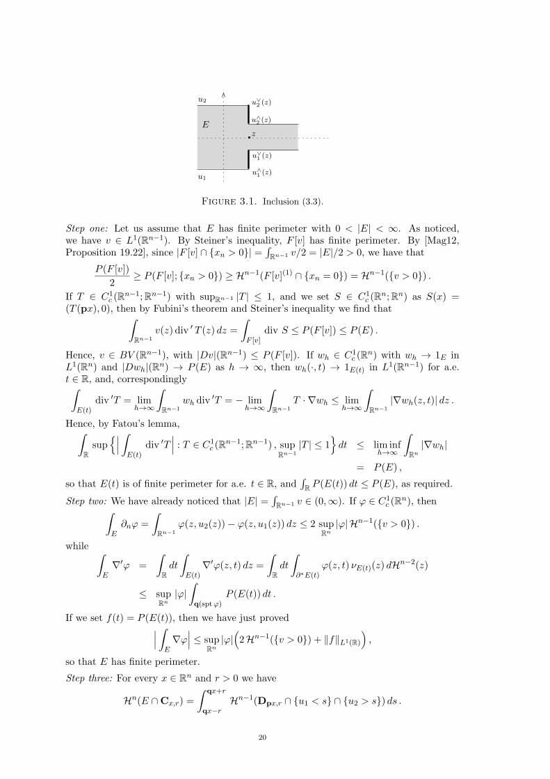
Moreover, see Figure 3.1,

(∂eE)z ⊂ [u∧1 (z), u∨1 (z)] ∪ [u∧2 (z), u

∨2 (z)] , ∀z ∈ Rn−1 , (3.3)

and (Su1 ∪ Su2

)\(u∨2 = u∨1 ∩ u∧2 = u∧1

)(3.4)

is countably Hn−2-rectifiable, with v∨ = 0 ⊆ u∨2 = u∨1 ∩ u∧2 = u∧1 .

Proof. We first notice that, if we set E(t) = z ∈ Rn−1 : (z, t) ∈ E, then we haveE(t) = u1 < t < u2 for every t ∈ R, and that, by Fubini’s theorem, E has finite volumeif and only if v ∈ L1(Rn−1); in both cases |E| =

∫Rn−1 v.

19

z

u1

u2 u∨2 (z)

E

u∨1 (z)

u∧2 (z)

u∧1 (z)

Figure 3.1. Inclusion (3.3).

Step one: Let us assume that E has finite perimeter with 0 < |E| < ∞. As noticed,we have v ∈ L1(Rn−1). By Steiner’s inequality, F [v] has finite perimeter. By [Mag12,Proposition 19.22], since |F [v] ∩ xn > 0| =

∫Rn−1 v/2 = |E|/2 > 0, we have that

P (F [v])

2≥ P (F [v]; xn > 0) ≥ Hn−1(F [v](1) ∩ xn = 0) = Hn−1(v > 0) .

If T ∈ C1c (Rn−1;Rn−1) with supRn−1 |T | ≤ 1, and we set S ∈ C1

c (Rn;Rn) as S(x) =(T (px), 0), then by Fubini’s theorem and Steiner’s inequality we find that∫

Rn−1

v(z) div ′ T (z) dz =

∫F [v]

div S ≤ P (F [v]) ≤ P (E) .

Hence, v ∈ BV (Rn−1), with |Dv|(Rn−1) ≤ P (F [v]). If wh ∈ C1c (Rn) with wh → 1E in

L1(Rn) and |Dwh|(Rn) → P (E) as h → ∞, then wh(·, t) → 1E(t) in L1(Rn−1) for a.e.t ∈ R, and, correspondingly∫

E(t)div ′T = lim

h→∞

∫Rn−1

wh div′T = − lim

h→∞

∫Rn−1

T · ∇wh ≤ limh→∞

∫Rn−1

|∇wh(z, t)| dz .

Hence, by Fatou’s lemma,∫Rsup

∣∣∣ ∫E(t)

div ′T∣∣∣ : T ∈ C1

c (Rn−1;Rn−1) , supRn−1

|T | ≤ 1dt ≤ lim inf

h→∞

∫Rn

|∇wh|

= P (E) ,

so that E(t) is of finite perimeter for a.e. t ∈ R, and∫R P (E(t)) dt ≤ P (E), as required.

Step two: We have already noticed that |E| =∫Rn−1 v ∈ (0,∞). If φ ∈ C1

c (Rn), then∫E∂nφ =

∫Rn−1

φ(z, u2(z))− φ(z, u1(z)) dz ≤ 2 supRn

|φ|Hn−1(v > 0) .

while ∫E∇′φ =

∫Rdt

∫E(t)

∇′φ(z, t) dz =

∫Rdt

∫∂∗E(t)

φ(z, t) νE(t)(z) dHn−2(z)

≤ supRn

|φ|∫q(sptφ)

P (E(t)) dt .

If we set f(t) = P (E(t)), then we have just proved∣∣∣ ∫E∇φ

∣∣∣ ≤ supRn

|φ|(2Hn−1(v > 0) + ∥f∥L1(R)

),

so that E has finite perimeter.

Step three: For every x ∈ Rn and r > 0 we have

Hn(E ∩Cx,r) =

∫ qx+r

qx−rHn−1(Dpx,r ∩ u1 < s ∩ u2 > s) ds .

20

If qx > u∨2 (px), then given t ∈ (u∨2 (px),qx) and r < qx− t we find that

Hn(E ∩Cx,r) ≤ 2 rHn−1(Dpx,r ∩ u2 > t) = o(rn) ,

so that x ∈ E(0). By a similar argument, we show thatx ∈ Rn : qx > u∨2 (px)

∪x ∈ Rn : qx < u∧1 (px)

⊂ E(0) ,

x ∈ Rn : u∨1 (px) < qx < u∧2 (px)⊂ E(1) .

We thus conclude that, if x ∈ ∂eE, then u∧1 (px) ≤ qx ≤ u∨2 (px) and either qx ≤ u∨1 (px)or qx ≥ u∧2 (px).

Step four: Let I be a countable dense subset of R such that u1 < t < u2 is of finiteperimeter for every t ∈ I. We claim that

u∧2 > u∧1 ∩ Su1 ⊂∪t∈I

∂eu2 > t > u1 . (3.5)

Indeed, if minu∧2 (z), u∨1 (z) > t > u∧1 (z), then

θ(u2 > t, z) = 1 , θ∗(u1 < t, z) > 0 , θ∗(u1 < t, z) < 1 ,

which implies θ∗(u1 < t < u2, z) > 0 and that θ∗(u1 < t < u2, z) < 1, and thus(3.5). In particular, u∧2 > u∧1 ∩ Su1 is countably Hn−2-rectifiable. By entirely similararguments, one checks that the sets u∨2 > u∨1 ∩Su2 , S

cu1

∩Su2 and Su1 ∩Scu2

are includedin the set on the right-hand side of (3.5), and thus complete the proof of (3.4).

Step five: We prove that v∨ = 0 ⊆ u∨2 = u∨1 ∩ u∧2 = u∧1 . Indeed from the generalfact that (f + g)∨ ≤ f∨+ g∨, we obtain that 0 ≤ u∨2 −u∨1 ≤ (u2−u1)

∨ = v∨. At the sametime, 0 ≤ u∧2 − u∧1 = (−u1)∨ − (−u2)∨ ≤ (−u1 + u2)

∨ = v∨. Proof of Theorem 3.1. Step one: We first consider the case that u1, u2 ∈ BVloc(Rn−1). By[GMS98a, Section 4.1.5], Σu1 and Σu2 are of locally finite perimeter, with

∂∗Σu1 ∩(Scu1

× R)

=Hn−1

x ∈ Rn : u1(px) = qx

, (3.6)

∂∗Σu1 ∩(Su1 × R

)=Hn−1

x ∈ Rn : u∧1 (px) < qx < u∨1 (px)

, (3.7)

and, by similar arguments, with

Σ(1)u1

∩(Scu1

× R)

=Hn−1

x ∈ Rn : u1(px) < qx

, (3.8)

Σ(1)u1

∩(Su1 × R

)=Hn−1

x ∈ Rn : u∨1 (px) < qx

, (3.9)

(Σu2)(1) ∩(Scu2

× R)

=Hn−1

x ∈ Rn : u2(px) > qx

, (3.10)

(Σu2)(1) ∩(Su2 × R

)=Hn−1

x ∈ Rn : u∧2 (px) > qx

. (3.11)

Let us now recall that, by [Mag12, Theorem 16.3], if F1, F2 are sets of locally finiteperimeter, then

∂∗(F1 ∩F2) =Hn−1

(F

(1)1 ∩ ∂∗F2

)∪(F

(1)2 ∩ ∂∗F1

)∪(∂∗F1 ∩ ∂∗F2 ∩νF1 = νF2

); (3.12)

moreover, if F1 ⊂ F2, then νF1 = νF2 Hn−1-a.e. on ∂∗F1 ∩ ∂∗F2. Since u1 ≤ u2 impliesΣu2 ⊂ Σu1 and Σu2 = Rn \ Σu2 , so that µΣu2

= −µΣu2 , we thus find

νΣu1= −νΣu2 , Hn−1-a.e. on ∂∗Σu1 ∩ ∂∗Σu2 . (3.13)

By (3.12) and (3.13), since E = Σu1 ∩ Σu2 we find

∂∗E =Hn−1

(∂∗Σu1 ∩ (Σu2)(1)

)∪(∂∗Σu2 ∩ (Σu1)

(1)).

21

We now apply (3.6) to u1 and (3.10) to u2 to find(∂∗Σu1 ∩ (Σu2)(1)

)∩((Sc

u1∩ Sc

u2)× R

)=Hn−1

(z, u1(z)) : z ∈ (Sc

u1∩ Sc

u2) , u1(z) < u2(z)

. (3.14)

We combine (3.7) applied to u1 and (3.10) applied to u2 to find(∂∗Σu1 ∩ (Σu2)(1)

)∩((Su1 ∩ Sc

u2)× R

)=Hn−1

(z, t) : z ∈ (Su1 ∩ Sc

u2) , u∧1 (z) < t < minu∨1 (z), u2(z)

. (3.15)

We combine (3.7) applied to u1 and (3.11) applied to u2 to find(∂∗Σu1 ∩ (Σu2)(1)

)∩((Su1 ∩ Su2)× R

)=Hn−1

(z, t) : z ∈ (Su1 ∩ Su2) , u

∧1 (z) < t < minu∨1 (z), u∧2 (z)

. (3.16)

We finally apply (3.6) to u1 and (3.11) to u2 to find(∂∗Σu1 ∩ (Σu2)(1)

)∩((Sc

u1∩ Su2)× R

)=Hn−1

(z, u1(z)) : z ∈ (Sc

u1∩ Su2) , u1(z) < u∧2 (z)

. (3.17)

This gives, by (3.1),

Hn−1(∂∗Σu1 ∩ (Σu2)(1) ∩ (G× R)

)by (3.14) =

∫G∩u1<u2

√1 + |∇u1|2 dHn−1 + |Dcu1|

(G ∩ u1 < u2

)by (3.15) and (3.16) +

∫G∩Su1

(minu∨1 , u∧2 − u∧1

)+dHn−2 ,

where we have also taken into account that, as a consequence of (3.17), we simply have

Hn−1((∂∗Σu1 ∩ (Σu2)(1)

)∩((Sc

u1∩ Su2)× R

))= 0 ,

by [Fed69, 3.2.23]. Also, by symmetry,

Hn−1(∂∗Σu2 ∩ (Σu1)

(1) ∩ (G× R))

=

∫G∩u1<u2

√1 + |∇u2|2 dHn−1 + |Dcu2|

(G ∩ u1 < u2

)+

∫G∩Su2

(u∨2 −maxu∧2 , u∨1

)+dHn−2 .

In conclusion we have proved

P (E;G× R) =

∫G∩u1<u2

(√1 + |∇u1|2 +

√1 + |∇u2|2

)dHn−1

+|Dcu1|(G ∩ u1 < u2

)+ |Dcu2|

(G ∩ u1 < u2

)(3.18)

+

∫G∩(Su1∪Su2 )

(minu∨1 , u∧2 − u∧1

)++

(u∨2 −maxu∧2 , u∨1

)+dHn−2 .

22

We thus deduce (3.2) by means of (3.18) and thanks to the identity,

min2(u2 − u1), [u1] + [u2]

= min

u∨2 + u∧2 − (u∨1 + u∧1 ), u

∨1 − u∧1 + u∨2 − u∧2

= u∨2 − u∧1 +min

u∧2 − u∨1 , u

∨1 − u∧2

= u∨2 − u∧1 +minu∧2 , u∨1 −maxu∧2 , u∨1

=(minu∨1 , u∧2 − u∧1

)++

(u∨2 −maxu∧2 , u∨1

)+.

This completes the proof of the theorem in the case that u1, u2 ∈ BVloc(Rn−1).

Step two: We now address the general case. If u1, u2 ∈ GBV (Rn−1), then Σu1 and Σu2 aresets of locally finite perimeter by [CCDPM13, Proposition 3.1], and thus E is of locallyfinite perimeter. We now prove (3.2). To this end, since (3.2) is an identity between Borelmeasures on Rn−1, it suffices to consider the case that G is bounded. Given M > 0, letEM = ΣτM (u1) ∩ ΣτM (u2). Since τMui ∈ BVloc(Rn−1) for every M > 0, i = 1, 2, by stepone we find that EM is a set of locally finite perimeter, and that (3.2) holds true on EM

with τM (u1) and τM (u2) in place of u1 and u2. We are thus going to complete the proofof the theorem by showing that,

P (E;G× R) = limM→∞

P (EM ;G× R) , (3.19)∫G∩u1<u2

√1 + |∇ui|2 dHn−1 = lim

M→∞

∫G∩τM (u1)<τM (u2)

√1 + |∇τM (ui)|2 dHn−1 , (3.20)

|Dcui|(G ∩ u1 < u2

)= lim

M→∞|DcτM (ui)|

(G ∩ ˜τM (u1) < ˜τM (u2)

),(3.21)

and that∫G∩(Su1∪Su2 )

min2(u2 − u1), [u1] + [u2]

dHn−2 (3.22)

= limM→∞

∫G∩(SτM (u1)

∪SτM (u2))min

2( ˜τM (u2)− ˜τM (u1)), [τM (u1)] + [τM (u2)]

dHn−2 .

Let us set fM (a, b) = τM (b) − τM (a) for a, b ∈ R ∪ ±∞. By (2.6), we can write theright-hand side of (3.22) as

∫G hM dHn−2, where

hM = 1SτM (u1)∪SτM (u2)

γ(fM (u∨1 , u

∨2 ), fM (u∧1 , u

∧2 ), fM (u∧1 , u

∨1 ), fM (u∧2 , u

∨2 )),

for a function γ : R×R×R×R → [0,∞) that is increasing in each of its arguments. Since,for every a, b ∈ R ∪ ±∞ with a ≤ b, the quantity fM (a, b) is increasing in M , with

limM→∞

fM (a, b) =

0 , if a = b = +∞ or a = b = −∞ ,b− a , if else ,

we see that SτM (ui)M>0 is a monotone increasing family of sets whose union is Sui ,

hMM>0 is an increasing family of functions on Rn−1, and that

limM→∞

hM = 1Su1∪Su2min

2(u2 − u1), [u1] + [u2]

,

where the convention that u2 − u1 = 0 if u2 = u1 = +∞ was also taken into account; wehave thus completed the proof of (3.22). Similarly, on noticing that

˜τM (u1) < ˜τM (u2) = fM (u∨1 , u∨2 ) + fM (u∧1 , u

∧2 ) > 0

= fM (u∨1 , u∨2 ) > 0 ∪ fM (u∧1 , u

∧2 ) > 0 ,

23

we see that ˜τM (u1) < ˜τM (u2)M>0 is a monotone increasing family of sets whose unionis u∨2 > u∨1 ∪ u∧2 > u∧1 . Therefore, by definition of |Dcui|, we find, for i = 1, 2,

limM→∞

|DcτMui|(G ∩ ˜τM (u1) < ˜τM (u2)

)= |Dcui|

(G ∩ (u∨2 > u∨1 ∪ u∧2 > u∧1 )

)= |Dcui|

(G ∩ u1 < u2

),

where in the last identity we have taken into account that Su1 ∪ Su2 is countably Hn−2-rectifiable, and thus |Dcui|-negligible for i = 1, 2. This proves (3.21). Next, we noticethat

|∇τM (ui)| = 1|ui|<M |∇ui| , Hn−1-a.e. on Rn−1 ,

so that (3.20) follows again by monotone convergence. By (3.2) applied to EM this showsin particular that the limit as M → ∞ of P (EM ;G×R) exists in [0,∞]. Thus, in order toprove (3.19) it suffices to show that P (E;G×R) is the limit of P (EMh

;G×R) as h→ ∞,where Mhh∈N has been chosen in such a way that

limh→∞

Hn−1(E(1) ∩ |xn| =Mh

)= 0 , Hn−1

(∂eE ∩ |xn| =Mh

)= 0 , ∀h ∈ N .

(3.23)(Notice that the choice of Mhh∈N is made possible by the fact that |E| < ∞, and sinceHn−1x∂eE is a Radon measure.) Indeed, by EM = E ∩ |xn| < M, by (3.23), and by[Mag12, Theorem 16.3], we have that

∂eEMh=

(|xn| < Mh ∩ ∂eE

)∪(|xn| =Mh ∩ E(1)

), ∀h ∈ N ,

so that, by the first identity in (3.23) we find P (E;G× R) = limh→∞ P (EMh;G× R), as

required. This completes the proof of the theorem.

In practice, we shall always apply Theorem 3.1 in situations where the sets under con-sideration are described in terms of their barycenter and slice length functions.

Corollary 3.3. If v ∈ (BV ∩ L∞)(Rn−1; [0,∞)), b ∈ GBV (Rn−1), and

W =W [v, b] =x ∈ Rn : |qx− b(px)| < v(px)

2

, (3.24)

then u1 = b − (v/2) ∈ GBV (Rn−1), u2 = b + (v/2) ∈ GBV (Rn−1), W is a set of locallyfinite perimeter with finite volume, and for every Borel set G ⊂ Rn−1 we have

P (W ;G× R) =

∫G∩v>0

√1 +

∣∣∣∇(b+

v

2

)∣∣∣2 +√1 +

∣∣∣∇(b− v

2

)∣∣∣2 dHn−1 (3.25)

+

∫G∩(Sv∪Sb)

minv∨ + v∧,max

[v], 2 [b]

dHn−2

+∣∣∣Dc

(b+

v

2

)∣∣∣(G ∩ v > 0)+

∣∣∣Dc(b− v

2

)∣∣∣(G ∩ v > 0),

where this identity holds true in [0,∞].

Proof. It is easily seen that (BV ∩L∞)+GBV ⊂ GBV . By Theorem 3.1, W = Σu1 ∩Σu2

is of locally finite perimeter, and P (W ;G × R) can be computed by means of (3.2) forevery Borel set G ⊂ Rn−1. We are thus left to prove that, Hn−2-a.e. on Su1 ∪ Su2 ,

min2(u2 − u1), [u1] + [u2]

= min

v∨ + v∧,max

[v], 2 [b]

. (3.26)

24

On Ju1 ∩ Ju2 ∩ νu1 = νu2 we have that

b∨ =u∨1 + u∨2

2, v∨ = max

u∨2 − u∨1 , u

∧2 − u∧1

,

b∧ =u∧1 + u∧2

2, v∧ = min

u∨2 − u∨1 , u

∧2 − u∧1

,

while on Ju1 ∩ Ju2 ∩ νu1 = −νu2 we find

b∨ = maxu∨2 + u∧1

2,u∧2 + u∨1

2

, v∨ = u∨2 − u∧1 ,

b∧ = minu∨2 + u∧1

2,u∧2 + u∨1

2

, v∧ = u∧2 − u∨1 ,

so that (3.26) is proved through an elementary case by case argument on Ju1 ∩ Ju2 , andthus, Hn−2-a.e. on Su1 ∩ Su2 . At the same time, on Su1 ∩ Sc

u2we have

b∨ =u2 + u∨1

2, v∨ = u2 − u∧1 ,

b∧ =u2 + u∧1

2, v∧ = u2 − u∨1 ,

from which we easily deduce (3.26) on Su1 ∩ Scu2; by symmetry, we notice the validity of

(3.26) on Scu1

∩ Su2 , and thus conclude the proof of the corollary.

Corollary 3.4. Let v : Rn−1 → [0,∞) be Lebesgue measurable. Then, F [v] is of finiteperimeter and volume if and only if v ∈ BV (Rn−1; [0,∞)) and Hn−1(v > 0) < ∞. Inthis case, if F = F [v], then for every z ∈ Rn−1 we have(

− v∧(z)

2,v∧(z)

2

)⊂ (F (1))z ⊂

[− v∧(z)

2,v∧(z)

2

], (3.27)

t ∈ R :v∧(z)

2< |t| < v∨(z)

2

⊂ (∂eF )z ⊂

t ∈ R :

v∧(z)

2≤ |t| ≤ v∨(z)

2

, (3.28)

while, for every Borel set G ⊂ Rn−1,

P (F ;G× R) = 2

∫G∩v>0

√1 +

∣∣∣∇v2

∣∣∣2 dHn−1 +

∫G∩Sv

[v] dHn−2 + |Dcv|(G) . (3.29)

Proof. By Proposition 3.2 and the coarea formula (2.15), we see that F [v] is of finiteperimeter if and only if v ∈ BV (Rn−1; [0,∞)) and Hn−1(v > 0) <∞. By arguing as instep three of the proof of Proposition 3.2, we easily prove (3.27) and (3.28). Finally, byapplying Theorem 3.1 to u2 = v/2 and u1 = −v/2, we prove (3.29) with |Dcv|(G∩v > 0)in place of |Dcv|(G). We conclude the proof of the corollary by Lemma 2.2.

We close this section with the proof of Proposition 1.5.

Proof of Proposition 1.5. We want to prove that, if λ ∈ [0, 1] \ 1/2 and

E =x ∈ Rn : −λ v2(px)−

v1(px)

2≤ qx ≤ v1(px)

2+ (1− λ) v2(px)

, (3.30)

then E ∈ M(v) and Hn(E∆(t en + F [v])) > 0 for every t ∈ R. By Corollary 3.4,

P (F [v]) = 2

∫Rn−1

√1 +

∣∣∣∇(v12

)∣∣∣2 + |Dsv2|(Rn−1) . (3.31)

25

At the same time, E = W [v, b], where b = ((1/2)− λ) v2. Since Dsv1 = 0, Dav2 = 0, and

v∨ + v∧ ≥ [v] = [v2] ≥ 2[b] Hn−2-a.e. on Rn−1, we easily find

∇(b± v

2

)= ±∇

(v12

), Hn−1-a.e. on Rn−1 ,

minv∨ + v∧,max

[v], 2 [b]

= [v2] , Hn−2-a.e. on Rn−1 ,

Dc(b+

v

2

)= (1− λ)Dcv2 , Dc

(b− v

2

)= −λDcv2 .

Since Sb ∪Sv =Hn−2 Sv2 , we find P (E) = P (F [v]) by (3.31) and (3.25). At the same time,

Hn(E∆(t en + F [v])) = 2

∫v>0

∣∣∣t− (12− λ

)v2

∣∣∣ dHn−1 , ∀t ∈ R ,

so that Hn(E∆(t en + F [v])) > 0 as λ = 1/2 and v2 is non-constant on v > 0.

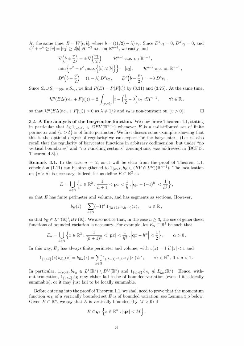
3.2. A fine analysis of the barycenter function. We now prove Theorem 1.1, statingin particular that bE 1v>δ ∈ GBV (Rn−1) whenever E is a v-distributed set of finiteperimeter and v > δ is of finite perimeter. We first discuss some examples showing thatthis is the optimal degree of regularity we can expect for the barycenter. (Let us alsorecall that the regularity of barycenter functions in arbitrary codimension, but under “novertical boundaries” and “no vanishing sections” assumptions, was addressed in [BCF13,Theorem 4.3].)

Remark 3.1. In the case n = 2, as it will be clear from the proof of Theorem 1.1,conclusion (1.11) can be strengthened to 1v>δ bE ∈ (BV ∩ L∞)(Rn−1). The localization

on v > δ is necessary. Indeed, let us define E ⊂ R2 as

E =∪h∈N

x ∈ R2 :

1

h+ 1< px <

1

h,∣∣∣qx− (−1)h

∣∣∣ < 1

h2

,

so that E has finite perimeter and volume, and has segments as sections. However,

bE(z) =∑h∈N

(−1)h 1((h+1)−1,h−1)(z) , z ∈ R ,

so that bE ∈ L∞(R)\BV (R). We also notice that, in the case n ≥ 3, the use of generalizedfunctions of bounded variation is necessary. For example, let Eα ⊂ R3 be such that

Eα =∪h∈N

x ∈ R3 :

1

(h+ 1)2< |px| < 1

h2,∣∣∣qx− hα

∣∣∣ < 1

2

, α > 0 .

In this way, Eα has always finite perimeter and volume, with v(z) = 1 if |z| < 1 and

1v>δ(z) bEα(z) = bEα(z) =∑h∈N

1((h+1)−2,h−2)(|z|)hα , ∀z ∈ R2 , 0 < δ < 1 .

In particular, 1v>δ bE2 ∈ L1(R2) \ BV (R2) and 1v>δ bE4 ∈ L1loc(R2). Hence, with-

out truncation, 1v>δ bE may either fail to be of bounded variation (even if it is locallysummable), or it may just fail to be locally summable.

Before entering into the proof of Theorem 1.1, we shall need to prove that the momentumfunction mE of a vertically bounded set E is of bounded variation; see Lemma 3.5 below.Given E ⊂ Rn, we say that E is vertically bounded (by M > 0) if

E ⊂Hn

x ∈ Rn : |qx| < M

.

26

Lemma 3.5. If v ∈ BV (Rn−1; [0,∞)) and E is a vertically bounded, v-distributed set offinite perimeter, then mE ∈ (BV ∩ L∞)(Rn−1), where

mE(z) =

∫Ez

t dH1(t) , ∀z ∈ Rn−1 .

Proof. If E is vertically bounded by M > 0, then v ∈ L∞(Rn−1), |mE | ≤ M v, andmE ∈ L∞(Rn−1). Moreover, mE ∈ BV (Rn−1) as, for every φ ∈ C1

c (Rn−1),∫Rn−1

mE ∇′φdHn−1 =

∫E∇′(φ(px)qx) dHn(x) =

∫∂∗E

φ(px)qxpνE(x) dHn−1(x)

≤ M supRn−1

|φ|P (E) .

Proof of Theorem 1.1. Step one: Let us decompose z ∈ Rn−1 as z = (z1, z′) ∈ R × Rn−2.

For every fixed z′ ∈ Rn−2, f : Rn−1 → R, G ⊂ Rn−1, and E ⊂ Rn, we define

fz′: R → R , fz

′(z1) = f(z1, z

′) ,

Gz′ = z1 ∈ R : (z1, z) ∈ G ,Ez′ = (z1, t) ∈ R2 : (z1, z

′, t) ∈ E .We now consider v and E as in the statement, and identify a set I ⊂ (0, 1) such thatH1((0, 1) \ I) = 0 and if δ ∈ I, then v > δ is a set of finite perimeter. We now fix δ ∈ I,and consider a set J ⊂ Rn−2 (depending on δ, and whose existence is a consequence of

Theorem C in section 4.4) such that Hn−2(Rn−2 \ J) = 0 and, for every z′ ∈ J , Ez′ is a

set of finite perimeter in R2 (hence, vz′ ∈ BV (R)) and

v > δz′ = vz′ > δis a set of finite perimeter in R. As we shall see in step three, for every z′ ∈ J ,∣∣∣D (

τM

(1vz′>δ bEz′

))∣∣∣(R) ≤ C(M, δ)P(vz

′> δ

)+ P (Ez′)

.

If we thus take into account that(τM

(1v>δ bE

))z′

= τM

(1vz′>δ bEz′

),

we thus conclude that∫Rn−2

∣∣∣∣D((τM

(1v>δ bE

))z′)∣∣∣∣(R) dHn−2(z′)

≤ C(M, δ)

∫Rn−2

P (vz′ > δ) + P (Ez′)

dHn−2(z′)

≤ C(M, δ)P (v > δ) + P (E)

,

where in the last step we have used [Mag12, Proposition 14.5]. We can repeat this argumentalong each coordinate direction in Rn−1 and combine it with [AFP00, Remark 3.104] toconclude that τM (1v>δ bE) ∈ (BV ∩ L∞)(Rn−1), with∣∣∣D(

τM

(1v>δ bE

))∣∣∣(Rn−1) ≤ C(M, δ)P (v > δ) + P (E)

.

The proof of (1.11) will then be completed in the following two steps.

Step two: Let n = 2. We claim that P (Es) < ∞ implies v ∈ L∞(R), while P (E) < ∞implies bE ∈ L∞(v > σ) for every σ > 0. The first claim follows by Corollary 3.4:indeed, P (Es) < ∞ implies v ∈ BV (R), and thus, trivially, v ∈ L∞(R). To prove thesecond claim, let us recall from step two in the proof of [Mag12, Theorem 19.15] that ifa, b ∈ R are such that a = b and

H1(E(1)a ) +H1(E

(1)b ) <∞ , H1(E(1)

a ∩ E(1)b ) = 0 , H1(∂∗E(1)

a ) = H1(∂∗E(1)b ) = 0 ,

27

then one has

H1(E(1)a ) +H1(E

(1)b ) ≤ P (E; a < x1 < b) . (3.32)

Should bE fail to be essentially bounded on v > σ for some σ > 0, then we may construct

a strictly increasing sequence ahh∈N ⊂ R with σ ≤ H1(E(1)ah ) <∞, H1(∂∗E

(1)ah ) = 0, and

H1(E(1)ah ∩ E(1)

ak ) = 0 if h = k. Correspondingly, by (3.32), we would get

2σ ≤ P (E; ah < x1 < ah+1) , ∀h ∈ N ,

and thus conclude that P (E) = +∞.

Step three: Let v ∈ BV (R), E be a v-distributed set of finite perimeter in R2 such thatEz is a segment for H1-a.e. z ∈ R, and let δ > 0 be such that v > δ is a set of finiteperimeter in R. According to step one, in order to complete the proof of (1.11) we are leftto show that, if M > 0, then∣∣∣D (

τM

(1v>δ bE

))∣∣∣(R) ≤ C(M, δ)P (v > δ) + P (E)

. (3.33)

By step two, v ∈ L∞(R) and bE ∈ L∞(v > δ). In particular, E is vertically boundedabove v > δ, that is, there exists L(δ) > 0 such that

E(δ) = E ∩(v > δ × R

)⊂H2

x ∈ R2 : v(px) > δ , |qx| < L(δ)

. (3.34)

Let us now set vδ = 1v>δ v. Since v > δ is of finite perimeter, we have

vδ ∈ (BV ∩ L∞)(R) , vδ > 0 = v > δ .

Concerning E(δ), we notice that, since v > δ×R is of locally finite perimeter, then E(δ)is, at least, a vδ-distributed set of locally finite perimeter such that E(δ)z is a segment for

H1-a.e. z ∈ R. But in fact, (3.34) implies |xn| > L(δ) ⊂ E(δ)(0), while at the same timewe have the inclusion

∂eE(δ) ⊂[∂eE ∩

(v > δ(1) × R

)]∪[(∂ev > δ × R

)∩(E(1) ∪ ∂eE

)];

in particular, E(δ) is of finite perimeter by Federer’s criterion, as

Hn−1(∂eE(δ)) ≤ P (E; v > δ(1) × R) + 2L(δ)P (v > δ) .

We now notice that bE(δ) = 1v>δ bE ∈ L∞(R), with P (E(δ); v > δ(1) × R) ≤ P (E);hence, (3.33) follows by showing∣∣∣D (

τM (bE(δ)))∣∣∣(R) ≤ C(M, δ)

P (vδ > 0) + P

(E(δ); vδ > 0(1) × R

),

for every M > 0. It is now convenient to reset notation.

Step four: As shown in step three, the proof of (1.11) is completed by showing that ifv ∈ (BV ∩ L∞)(R) is such that, for some δ > 0, v > 0 = v > δ is a set of finiteperimeter in R, and E is a vertically bounded, v-distributed set of finite perimeter in R2

with bE ∈ L∞(R), then, for every M > 0,

|D (τM (bE))|(R) ≤ C(M, δ)P (v > 0) + P

(E; v > 0(1) × R

). (3.35)

We start by noticing that, since E is vertically bounded, then by Lemma 3.5 we havemE ∈ (BV ∩ L∞)(R). Moreover, if we set

w =1v>0

v=

1v>δ

v,

28

then we have w ∈ (BV ∩ L∞)(R), and thus bE = wmE ∈ (BV ∩ L∞)(R). We now notice

that, since v = 0 ⊂ τM (bE) = 0, we have v = 0(1) ⊂ τM (bE) = 0(1); at the sametime, a simple application of the co-area formula shows that

0 = |D(τM (bE))|(τM (bE) = 0(1)

)≥ |D(τM (bE))|

(v = 0(1)

)= |D(τM (bE))|

(v > 0(0)

). (3.36)

Moreover, since v > 0 is a set of finite perimeter, we know that ∂ev > 0 is a finite set,so that

|D(τM (bE))|(∂ev > 0

)=

∫SτM (bE)∩∂ev>0

[τM (bE)] dH0 ≤ 2M P (v > 0) , (3.37)

where we have noticed that [τM (bE)] ≤ 2M since |τM (bE)| ≤ M on Rn−1. By (3.36) and(3.37), in order to achieve (3.35), we are left to prove that

|D (τM (bE))|(v > 0(1)

)≤ C(M, δ)P

(E; v > 0(1) × R

). (3.38)

By (2.9) and by v > δ = v > 0 we have

v∧ > 0 ⊂ v > 0(1) = v > δ(1) ⊂ v∧ ≥ δ ⊂ v∧ > 0 ,

that is v > 0(1) = v∧ > 0. By applying Corollary 3.3 to G = v > 0(1) = v∧ > 0,

P (E; v > 0(1) × R) (3.39)

=

∫v>0

√1 +

∣∣∣(bE +v

2

)′∣∣∣2 +√1 +

∣∣∣(bE − v

2

)′∣∣∣2 dH1

+

∫v>0(1)∩(Sv∪SbE

)min

v∨ + v∧,max

[v], 2 [bE ]

dH0

+∣∣∣Dc

(bE +

v

2

)∣∣∣(v∧ > 0 ∩ v > 0)+

∣∣∣Dc(bE − v

2

)∣∣∣(v∧ > 0 ∩ v > 0).

Since v∧ = 0 = v = 0 ∪ v∨ > 0 = v∧ where v∨ > 0 = v∧ ⊂H0 Jv, we find thatv∧ = 0 is |Dcf |-equivalent to v = 0 for every f ∈ BVloc(Rn−1): hence,∣∣∣Dc

(bE ± v

2

)∣∣∣(v∧ > 0 ∩ v > 0)=

∣∣∣Dc(bE ± v

2

)∣∣∣(v∧ > 0). (3.40)

By (3.39), (3.40), the triangular inequality, and as v∧ ≥ δ on v > 0(1) = v > δ(1),

P (E; v > 0(1) × R) ≥ 2

∫v>0

|b′E | dH1 + 2

∫v>0(1)∩SbE

minδ, [bE ] dH0

+2 |DcbE |(v∧ > 0) . (3.41)

At the same time, by [AFP00, Theorem 3.99], for every M > 0 we have

|D(τM (bE))|(v > 0(1)) (3.42)

=

∫|bE |<M∩v>0

|b′E | dH1 + |DcbE |(

|bE | < M∩ v > 0(1)

)+

∫SbE

∩b∧E<M∩b∨E>−M∩v>0(1)minM, b∨E −max−M, b∧E dH0 .

As it is easily seen by arguing on a case by case basis,

minM, b∨E −max−M, b∧E ≤ max1,

2M

δ

minδ, [bE ] , on SbE . (3.43)

By combining (3.41), (3.42), and (3.43) we conclude the proof of (3.38), thus of step four.The proof of (1.11) is now complete.

29

Step five: Since v > δ is of finite perimeter for a.e. δ > 0, we find that, correspond-ingly, bδ = 1v>δ bE ∈ GBV (Rn−1) for a.e. δ > 0. In particular, bδ is approximately

differentiable at Hn−1-a.e. x ∈ Rn−1. Since bδ = bE on v > δ, by (2.12) it follows that

∇bE(x) = ∇bδ(x) , Hn−1-a.e. x ∈ v > δ . (3.44)

By considering δh → 0 as h → ∞ with v > δh of finite perimeter for every h ∈ N, wefind that bE is approximately differentiable at Hn−1-a.e. x ∈ v > 0. Since, trivially, bEis approximately differentiable at every x ∈ v = 0(1) with ∇bE(x) = 0, we conclude thatbE is approximately differentiable at Hn−1-a.e. x ∈ Rn−1. By [AFP00, Theorem 4.34], forevery Borel G ⊂ Rn−1 we have∫

RHn−2(G ∩ ∂ebδ > t) dt =

∫G|∇bδ| dHn−1 +

∫G∩Sbδ

[bδ] dHn−2 + |Dcbδ|(G) . (3.45)

Let us notice that, by (2.10), [bδ] = [bE ] on v > δ(1), and thus Sbδ ∩ v > δ(1) =

SbE ∩ v > δ(1). By (3.44) and by applying (3.45) to G ∩ v > δ(1) where G ⊂ Rn−1 isa Borel set, we find∫

RHn−2(G ∩ v > δ(1) ∩ ∂ebδ > t) dt (3.46)

=

∫G∩v>δ

|∇bE | dHn−1 +

∫G∩SbE

∩v>δ(1)[bE ] dHn−2 + |Dcbδ|(G ∩ v > δ(1)) .

Since τMbδ = 1v>δ τMbδ, by applying Lemma 2.3 we find that, for every G ⊂ Rn−1,

|Dcbδ|(G∩v > δ(1)) = limM→∞

|DcτMbδ|(G∩v > δ(1)) = limM→∞

|DcτMbδ|(G) = |Dcbδ|(G) .(3.47)

At the same time, since v > δ ∩ bδ > t = v > δ ∩ bE > t for every t ∈ R, we have

v > δ(1) ∩ ∂ebδ > t = v > δ(1) ∩ ∂ebE > t , ∀t ∈ R ,

and thus∫RHn−2(G ∩ v > δ(1) ∩ ∂ebδ > t) dt =

∫RHn−2(G ∩ v > δ(1) ∩ ∂ebE > t) dt .

If we now set δ = δh into (3.46) and then let h→ ∞, then by

v∧ > 0 =∪h∈N

v > δh(1) , (3.48)

(which follows by (2.9)), by (3.47), and thanks to the definition (1.13) of |DcbE |+, wefind that (1.12) holds true for every Borel set G ⊂ v∧ > 0, as required. We have thuscompleted the proof of Theorem 1.1.

3.3. Characterization of equality cases, part one. In this section we prove the nec-essary conditions for equality cases in Steiner’s inequality stated in Theorem 1.2. Wepremise the following simple lemma to the proof.

Lemma 3.6. If µ and ν are Rn−1-valued Radon measures on Rn−1, then

2 |µ|(G) ≤ |ν + µ|(G) + |ν − µ|(G) , (3.49)

for every Borel set G ⊂ Rn−1. Moreover, equality holds in (3.49) for every bounded Borelset G ⊂ Rn−1 if and only if there exists a Borel function f : Rn−1 → [−1, 1] with

ν(G) =

∫Gf dµ , for every bounded Borel set G ⊂ Rn−1.

30

Proof. The validity of (3.49) follows immediately from the fact that if G is a Borel set inRn−1, then |µ|(G) is the supremum of the sums

∑h∈N |µ(Gh)| along partitions Ghh∈N of

G into bounded Borel sets. From the same fact, we immediately deduce that |ν+µ|(G) =|ν − µ|(G) = |ν|(G) whenever |µ|(G) = 0: therefore, if G is such that |µ|(G) = 0 and(3.49) holds as an equality, then |ν|(G) = 0. In particular, if equality holds in (3.49) forevery bounded Borel set G ⊂ Rn−1, then |ν| is absolutely continuous with respect to |µ|.By the Radon-Nykodım theorem we have that ν = g d|µ| for a |µ|-measurable functiong : Rn−1 → Rn−1, as well as µ = h d|µ|, for a |µ|-measurable function h : Rn−1 → Sn−2.In particular ν ± µ = (g ± h) d|µ|, and thus, since equality holds in (3.49),

2|µ|(G) = |ν + µ|(G) + |ν − µ|(G) =∫G|g + h| d|µ|+

∫G|g − h| d|µ| ,

for every Borel set G ⊂ Rn−1, which gives

|g + h|+ |h− g| = 2 = 2|h| , |µ|-a.e. on Rn−1 .

Thus, there exists λ : Rn−1 → [0,∞) such that (h− g) = λ (g + h) |µ|-a.e. on Rn−1, i.e.

g =1− λ

1 + λh , |µ|-a.e. on Rn−1 .

This proves that ν = f dµ where f = (1 − λ)/(1 + λ). By Borel regularity of |µ|, we canassume without loss of generality that f is Borel measurable. The proof is complete.

Proof of Theorem 1.2, necessary conditions. Let E ∈ M(v). By Theorem A, we havethat Ez is H1-equivalent to a segment for Hn−1-a.e. z ∈ Rn−1, that is (1.15). As aconsequence, by Theorem 1.1, we have bδ = 1v>δ bE ∈ GBV (Rn−1) whenever v > δ isof finite perimeter. Let us set

I =δ > 0 : v > δ and v < δ are sets of finite perimeter

, (3.50)

Jδ =M > 0 : bδ < M and bδ > −M are sets of finite perimeter

, (3.51)

and notice that H1((0,∞) \ I) = 0 since v ∈ BV (Rn−1), and that H1((0,∞) \ Jδ) = 0for every δ ∈ I, as bδ ∈ GBV (Rn−1) whenever δ ∈ I. By taking total variations in(1.18), we find 2 |Dc(τMbδ)|(G) ≤ |Dcv|(G) for every bounded Borel set G ⊂ Rn−1. Byletting first M → ∞ (in Jδ) and then δ → 0 (in I) we prove (1.19). Let us also noticethat (1.20) is an immediate corollary of (1.12) and (1.19), once (1.16), (1.17) have beenproved. Summarizing, these remarks show that we only need to prove the validity of(1.16), (1.17), and (1.18) (for δ ∈ I and M ∈ Jδ) in order to complete the proof of thenecessary conditions for equality cases. This is accomplished in various steps.

Step one: Let us fix δ, L ∈ I and M ∈ Jδ, and set

Σδ,L,M = δ < v < L ∩ |bE | < M = |bδ| < M ∩ δ < v < L ,

so that Σδ,L,M is a set of finite perimeter. Since τMbδ ∈ (BV ∩L∞)(Rn−1) (see the end ofstep one in the proof of Theorem 1.1), 1Σδ,L,M

∈ (BV ∩ L∞)(Rn−1), and τMbδ = bδ = bEon Σδ,L,M , we have

bδ,L,M = 1Σδ,L,MbE ∈ (BV ∩ L∞)(Rn−1) .

We now claim that there exists a Borel function fδ,L,M : Rn−1 → [−1/2, 1/2] such that

∇bδ,L,M (z) = 0 , for Hn−1-a.e. z ∈ Σδ,L,M , (3.52)

Dcbδ,L,M (G) =

∫Gfδ,L,M d (Dcv) , for every bounded Borel set G ⊂ Σ

(1)δ,L,M .(3.53)

31

Indeed, let us set vδ,L,M = 1Σδ,L,Mv. Since vδ,L,M , bδ,L,M ∈ (BV ∩ L∞)(Rn−1), we can

apply Corollary 3.3 to W =W [vδ,L,M , bδ,L,M ]. Since W [vδ,L,M , bδ,L,M ] = E ∩ (Σδ,L,M ×R),and thus

∂eE ∩ (Σ(1)δ,L,M × R) = ∂eW [vδ,L,M , bδ,L,M ] ∩ (Σ

(1)δ,L,M × R) ,

we find that, for every Borel set G ⊂ Σ(1)δ,L,M \ (Svδ,L,M

∪ Sbδ,L,M),

P (E;G× R) = P (W [vδ,L,M , bδ,L,M ];G× R)

=

∫G

√1 +

∣∣∣∇(bδ,L,M +

vδ,L,M2

)∣∣∣2 +√1 +

∣∣∣∇(bδ,L,M −

vδ,L,M2

)∣∣∣2 dHn−1

+∣∣∣Dc

(bδ,L,M +

vδ,L,M2

)∣∣∣(G) + ∣∣∣Dc(bδ,L,M −

vδ,L,M2

)∣∣∣(G) . (3.54)

By Lemma 2.3 applied with vδ,L,M = 1Σδ,L,Mv, we find that

∇vδ,L,M = 1Σδ,L,M∇v , Hn−1-a.e. on Rn−1 ,

Dcvδ,L,M = DcvxΣ(1)δ,L,M ,

Svδ,L,M∩ Σ

(1)δ,L,M = Sv ∩ Σ

(1)δ,L,M .

By (3.54), we thus find that

P (E;G× R) =

∫G

√1 +

∣∣∣∇(bδ,L,M +

v

2

)∣∣∣2 +√1 +

∣∣∣∇(bδ,L,M − v

2

)∣∣∣2 dHn−1

+∣∣∣Dc

(bδ,L,M +

v

2

)∣∣∣(G) + ∣∣∣Dc(bδ,L,M − v

2

)∣∣∣(G) , (3.55)

for every Borel set G ⊂ Σ(1)δ,L,M \ (Sv ∪ Sbδ,L,M

). By Corollary 3.4, for every Borel set

G ⊂ Rn−1,

P (F [v];G× R) = 2

∫G

√1 +

∣∣∣∇v2

∣∣∣2 dHn−1 +

∫G∩Sv

[v] dHn−2 + |Dcv|(G) . (3.56)

Taking into account that P (E;G × R) = P (F [v];G × R) for every Borel set G ⊂ Rn−1,

we combine (3.55) and (3.56), together with the convexity of ξ ∈ Rn−1 7→√

1 + |ξ|2 and

(3.49), to find that, if G ⊂ Σ(1)δ,L,M \ (Sv ∪ Sbδ,L,M

), then

0 =

∫G

√1 +

∣∣∣∇(bδ,L,M +

v

2

)∣∣∣2+√1 +

∣∣∣∇(bδ,L,M − v

2

)∣∣∣2−2

√1 +

∣∣∣∇v2

∣∣∣2 dHn−1 , (3.57)

0 =∣∣∣Dc

(bδ,L,M +

v

2

)∣∣∣(G) + ∣∣∣Dc(bδ,L,M − v

2

)∣∣∣(G)− |Dcv|(G) . (3.58)

Since Σ(1)δ,L,M \ (Sv ∪ Sbδ,L,M

) is Hn−1-equivalent to Σδ,L,M , by (3.57) and by the strict

convexity of ξ ∈ Rn−1 7→√

1 + |ξ|2, we come to prove (3.52). By applying Lemma 3.6 to

µ =Dcv

2, ν = Dcbδ,L,Mx

(Σ(1)δ,L,M \ (Sv ∪ Sbδ,L,M

))= Dcbδ,L,MxΣ(1)

δ,L,M ,

we prove (3.53). This completes the proof of (3.52) and (3.53).

Step two: We prove (1.18). Let δ, L ∈ I and M ∈ Jδ. Since bδ,L,M = 1Σδ,L,MτMbδ, by

Lemma 2.3 we have

Dcbδ,L,M = Dc(τMbδ)xΣ(1)δ,L,M .

We combine this fact with (3.53) to find a Borel function fδ,M : Rn−1 → [−1/2, 1/2] with

DcτMbδ(G) =

∫Gfδ,M d (Dcv) , for every bounded Borel set G ⊂ Σ

(1)δ,L,M .

32

As a consequence, the Radon measures DcτMbδ and fδ,M Dcv coincide on every boundedBorel set contained into∪

L∈IΣ(1)δ,L,M =

∪L∈I

v > δ(1) ∩ |bE | < M(1) ∩ v < L(1)

=(v > δ(1) ∩ |bE | < M(1)

)∩

∪L∈I

v < L(1)

= v > δ(1) ∩ |bE | < M(1) ∩ v∨ <∞ ,

where in the last identity we have used (2.8). Since Hn−2(v∨ = ∞) = 0 by [Fed69,4.5.9(3)], the set v∨ = ∞ is negligible with respect to both |DcτMbδ| and |Dcv|. We

have thus proved that, for every bounded Borel set G ⊂ v > δ(1) ∩ |bE | < M(1),

Dc(τMbδ)(G) =

∫Gfδ,M d (Dcv) . (3.59)

Since for every M ′ > M and δ′ < δ we have that τMbδ = τM ′bδ′ on v > δ ∩ |bE | < M,by Lemma 2.2 we obtain that

Dc(τMbδ)xv > δ(1) ∩ |bE | < M(1) = Dc(τM ′bδ′)xv > δ(1) ∩ |bE | < M(1) ,

and therefore (3.59) can be rewritten with a function f independent of M and δ; thus,

Dc(τMbδ)(G) =

∫Gf d (Dcv) , (3.60)

for every bounded Borel set G ⊂ v > δ(1) ∩|bE | < M(1). We next notice that, if δ ∈ Iand M ∈ Jδ, then

τM bδ =M 1bδ≥M −M 1bδ≤−M + 1|bδ|<M∩v>δτMbδ , on Rn−1 ,

is an identity between BV functions. By [AFP00, Example 3.97] we thus find

DcτMbδ = Dc(1|bδ|<M∩v>δτMbδ

)= 1(|bδ|<M∩v>δ)(1)D

c(τMbδ)

= Dc(τMbδ)x(|bδ| < M(1) ∩ v > δ(1)

). (3.61)

Since by (3.61) the measure Dc(τMbδ) is concentrated on v > δ(1) ∩ |bE | < M(1), wededuce from (3.60) that for every bounded Borel set G ⊂ Rn−1

Dc(τMbδ)(G) = Dc(τMbδ)(G ∩ v > δ(1) ∩ |bE | < M(1)

)=

∫G∩v>δ(1)∩|bE |<M(1)

f d (Dcv) ,

which proves (1.18).

Step three: We prove (1.16). Let δ, L ∈ I and M ∈ Jδ. Since bδ,L,M = bE on Σδ,L,M , by(3.52) and by (2.12) we find that ∇bE = 0 Hn−1-a.e. on Σδ,L,M . By taking a union firston M ∈ Jδ, and then on δ, L ∈ I, we find that ∇bE = 0 Hn−1-a.e. on v > 0. At thesame time bE = 0 on v = 0 by definition, and thus, again by (2.12), we have ∇bE = 0Hn−1-a.e. on v = 0. This completes the proof of (1.16).

Step four: We prove (1.17). We fix δ, L ∈ I and define Σδ,L = δ < v < L, bδ,L =1Σδ,L

bE , and vδ,L = 1Σδ,Lv. Since Σδ,L is a set of finite perimeter, it turns out that

bδ,L ∈ GBV (Rn−1), while, by construction, vδ,L ∈ (BV ∩ L∞)(Rn−1). We are in theposition to apply Corollary 3.3 to obtain a formula for the perimeter ofW [vδ,L, bδ,L] relative

to cylinders G × R for Borel sets G ⊂ Rn−1. In particular, if G ⊂ Σ(1)δ,L ∩ (Svδ,L ∪ Sbδ,L),

33

then

P (E;G× R) = P (W [vδ,L, bδ,L];G× R)

=

∫Gmin

v∨δ,L + v∧δ,L,max

[vδ,L], 2 [bδ,L]

dHn−2 .

Since, by (2.10), Σ(1)δ,L ∩ Svδ,L = Σ

(1)δ,L ∩ Sv with v∨δ,L = v∨, v∧δ,L = v∧, and [vδ,L] = [v] on

Σ(1)δ,L, we have

P (E;G× R) =∫Gmin

v∨ + v∧,max

[v], 2 [bδ,L]

dHn−2 ,

whenever G ⊂ Σ(1)δ,L ∩ (Sv ∪ Sbδ,L). Since P (E;G× R) = P (F [v];G× R), by (3.56),

minv∨ + v∧,max

[v], 2 [bδ,L]

= [v] , Hn−2-a.e. on (Sbδ,L ∪ Sv) ∩ Σ

(1)δ,L .

Since v∧ ≥ δ on Σ(1)δ,L, we deduce that v∨ + v∧ > [v] on Σ

(1)δ,L, and thus the above condition

immediately implies that

2 [bδ,L] ≤ [v] , Hn−2-a.e. on (Sbδ,L ∪ Sv) ∩ Σ(1)δ,L .

In particular, Sbδ,L ∩ Σ(1)δ,L ⊂Hn−2 Sv, and we have proved

2 [bδ,L] ≤ [v] , Hn−2-a.e. on Σ(1)δ,L .

By (2.10), [bδ,L] = [bE ] on Σ(1)δ,L. By taking the union of Σ

(1)δ,L on δ, L ∈ I, and by taking

(2.8) and (2.9) into account, we thus find that

2 [bE ] ≤ [v] , Hn−2-a.e. on v∧ > 0 ∪ v∨ <∞ .

Since, as noticed above, v∨ = ∞ is Hn−2-negligible, we have proved (1.17).

3.4. Characterization of equality cases, part two. We now complete the proof ofTheorem 1.2, by showing that if a v-distributed set of finite perimeter E satisfies (1.15),(1.16), (1.17), and (1.18), then E ∈ M(v). The following proposition will play a crucialrole.

Proposition 3.7. If v ∈ BV (Rn−1; [0,∞)), Hn−1(v > 0) <∞, and E is a v-distributedset of finite perimeter with section as segments, then

P (E; v∧ = 0 × R) = P (F [v]; v∧ = 0 × R) =∫v∧=0

v∨ dHn−2 . (3.62)

Remark 3.2. With Proposition 3.7 at hand, one can actually go back to Corollary 3.3 andobtain a formula for P (E;G× R) in terms of v and bE whenever E is a v-distributed setof finite perimeter with section as segments. Since such a formula may be of independentinterest, we have included its proof in Appendix B.

Proof of Proposition 3.7. Let I = t > 0 : v > t and v < t is of finite perimeter, sothat we have as usual H1((0,∞) \ I) = 0. Since∫ ∞

0P (v > t) dt =

∫ ∞

0P (v < t) dt = |Dv|(Rn−1) <∞ ,

we can find two sequences δhh∈N, Lhh∈N ⊂ I such that

limh→∞

δh = 0 , limh→∞

δh P (v > δh) = 0 , (3.63)

limh→∞

Lh = ∞ , limh→∞

Lh P (v < Lh) = 0 . (3.64)

34

Let us set Σh = Lh > v > δh and Eh = E∩(Σh×R). Notice that Eh is, trivially, a set of

locally finite perimeter. Since Eh locally converges to E as h→ ∞, since P (Eh; Σ(0)h ×R) =

0, and since ∂eEh ∩ (Σ(1)h × R) = ∂eE ∩ (Σ

(1)h × R) we have

P (E) ≤ lim infh→∞

P (Eh) = lim infh→∞

P (E; Σ(1)h × R) + P (Eh; ∂

eΣh × R) . (3.65)

By (2.8) and (2.9),

limh→∞

1Σ

(1)h

(z) = 1v∧>0∩v∨<∞(z) , ∀z ∈ Rn−1 ,

so that by dominated convergence and thanks to the fact that E has finite perimeter,

limh→∞

P (E; Σ(1)h × R) = P

(E;

(v∧ > 0 ∩ v∨ <∞

)× R

)= P (E; v∧ > 0 × R) .

(In the last identity we have first used [Fed69, 4.5.9(3)] to infer that Hn−2(v∨ = ∞) = 0,and then [Fed69, 2.10.45] to conclude that Hn−1(v∨ = ∞× R) = 0.) Hence, by (3.65),

P (E; v∧ = 0 × R) ≤ lim infh→∞

P (Eh; ∂eΣh × R) . (3.66)

Since δh, Lh ∈ I, we have vh = 1Σhv ∈ (BV ∩L∞)(Rn−1) and ah = 1Σh

bE ∈ GBV (Rn−1)(indeed, ah = 1v<Lh bδh where bδh = 1v>δh bE ∈ GBV (Rn−1) thanks to Theorem 1.1).Since Eh =W [vh, ah] according to (3.24), we can apply (3.25) in Corollary 3.3 to G = ∂eΣh

to find that

P (Eh; ∂eΣh × R) =

∫∂eΣh∩(Svh

∪Sah)min

v∨h + v∧h ,max[vh], 2[ah]

dHn−2 . (3.67)

(Notice that, since ∂eΣh is countablyHn−2-rectifiable, we are only interested in the “jump”contribution in (3.25).) Let us now set

K1h = ∂eΣh ∩ ∂ev > δh , K2

h = ∂eΣh \ ∂ev > δh ⊂ ∂ev < Lh .

The key remark to exploit (3.67) is that, as one can check with standard arguments,

v∨h = v∨ ≥ δh ≥ v∧ , v∧h = 0 , Hn−2-a.e. on K1h , (3.68)

v∨ ≥ Lh ≥ v∧ = v∨h , v∧h = 0 , Hn−2-a.e. on K2h . (3.69)

(For example, in order to prove (3.69), we argue as follows. First, we notice that we alwayshave v∨ ≥ Lh ≥ v∧ and v∧h = 0 on ∂ev < Lh. In particular, v = Lh on Sc

v ∩ ∂ev < Lh,and this immediately implies v∨h = Lh on Sc

v ∩ ∂ev < Lh. Finally, by taking intoaccount that vh = 1Σh

v with Σh ⊂ v < Lh, one checks that v∧ = v∨h Hn−2-a.e. onJv ∩ ∂∗v < Lh.) By (3.68) and (3.69) we have

minv∨h + v∧h ,max[vh], 2[ah] = v∨ , Hn−2-a.e. on K1h , (3.70)

minv∨h + v∧h ,max[vh], 2[ah] = v∧ , Hn−2-a.e. on K2h , (3.71)

so that, by (3.67), and since, again by (3.68), K1h ⊂Hn−2 Svh , we find

P (Eh; ∂eΣh × R) ≤

∫K1

h

v∨ dHn−2 +

∫K2

h

v∧ dHn−2 . (3.72)

By (3.69) and (3.64), we have

lim suph→∞

∫K2

h

v∧ dHn−2 ≤ lim suph→∞

LhHn−2(K2h) ≤ lim sup

h→∞Lh P (v < Lh) = 0 . (3.73)

We are now going to prove that

limh→∞

∫∂ev>δh

v∨ dHn−2 =

∫v∧=0

v∨ dHn−2 . (3.74)

35

(This will be useful in the estimate of the right-hand side of (3.67) as K1h ⊂ ∂ev > δh.)

Since v∧ = 0 ∩ ∂ev > δh = v∧ = 0 ∩ Sv ∩ ∂ev > δh = v∧ = 0 ∩ [v] ≥ δh, wehave that, monotonically as h→ ∞,

v∨ 1v∧=0∩∂ev>δh → v∨ 1v∧=0∩Sv, pointwise on Rn−1.

Hence,

limh→∞

∫v∧=0∩∂ev>δh

v∨ dHn−2 =

∫v∧=0∩Sv

v∨ dHn−2 =

∫v∧=0

v∨ dHn−2 . (3.75)

We now claim that

limh→∞

∫v∧>0∩∂ev>δh

v∨ dHn−2 = 0 . (3.76)

Indeed, since v∨ = v∧ = δh on Scv ∩ ∂ev > δh, we find that∫

Scv∩v∧>0∩∂ev>δh

v∨ dHn−2 ≤ δhHn−2(∂ev > δh) = δh P (v > δh) ,

so that, by (3.63),

lim suph→∞

∫v∧>0∩∂ev>δh

v∨ dHn−2

= lim suph→∞

∫Sv∩v∧>0∩∂ev>δh

v∨ dHn−2

= lim suph→∞

∫Sv∩v∧>0∩∂ev>δh

[v] + v∧ dHn−2

(by (3.68)) ≤ lim suph→∞

∫Sv∩v∧>0∩∂ev>δh

[v] dHn−2 + δhHn−2(∂ev > δh)

(by (3.63)) = lim suph→∞

∫Sv∩v∧>0∩∂ev>δh

[v] dHn−2 . (3.77)

Now, if z ∈ v∧ > 0, then z ∈ v > δ(1) for every δ < v∧(z), so that,

1Sv∩v∧>0∩∂ev>δh → 0 , pointwise on Rn−1 ,

as h→ ∞. Since [v] ∈ L1(Hn−2xSv), by dominated convergence we find

limh→∞

∫Sv∩v∧>0∩∂ev>δh

[v] dHn−2 = 0 . (3.78)

By combining (3.77) and (3.78), we prove (3.76). By (3.75) and (3.76), we deduce (3.74).By K1

h ⊂ ∂ev > δh, (3.72), (3.73), and (3.74), we deduce that

lim suph→∞

P (Eh; ∂eΣh × R) ≤

∫v∧=0

v∨ dHn−2 .

By combining this last inequality with (3.66) we find

P (E; v∧ = 0 × R) ≤∫v∧=0

v∨ dHn−2

= P (F [v]; v∧ = 0 × R) ≤ P (E; v∧ = 0 × R) ,

where the identity follows by (3.29), and the final inequality is, of course, (1.1). Thiscompletes the proof of (3.62).

36

Remark 3.3. Let v ∈ BV (Rn−1; [0,∞)) with Hn−1(v > 0) < ∞, and let E be a v-distributed set with segments as section. Then, E is of finite perimeter if and only ifsuph∈N P (Eh) <∞, where

Eh = E ∩ (Σh × R) , Σh = Lh > v > δh ,and δhh∈N, Lhh∈N ⊂ (0,∞) are such that

limh→∞

δh = 0 , limh→∞

δh P (v > δh) = 0 ,

limh→∞

Lh = ∞ , limh→∞

Lh P (v < Lh) = 0 .

The fact that P (E) <∞ implies suph∈N P (Eh) <∞ is implicit in the proof of Proposition3.7. Conversely, if Ehh∈N is defined as above, then Eh → E as h → ∞, and thussuph∈N P (Eh) <∞ implies P (E) <∞ by lower semicontinuity of perimeter.

Lemma 3.8. If v ∈ (BV ∩L∞)(Rn−1), b : Rn−1 → R is such that τMb ∈ (BV ∩L∞)(Rn−1)for a.e. M > 0, and µ is a Rn−1-valued Radon measure such that

limM→∞

|µ−DcτMb|(G) = 0 , for every bounded Borel set G ⊆ Rn−1 , (3.79)

then,

|Dc(b+ v)|(G) ≤ |µ+Dcv|(G) , for every Borel set G ⊆ Rn−1. (3.80)

Proof. Let us assume that |v| ≤ L Hn−1-a.e. on Rn−1. If f ∈ BV (Rn−1), then

τM f =M 1f>M −M 1f<−M + 1|f |<MτMf ∈ (BV ∩ L∞)(Rn−1) ,

for every M such that f > M and f < −M are of finite perimeter, and thus, by[AFP00, Example 3.97],

DcτMf = Dc(1|f |<MτMf

)= 1|f |<M(1)D

c(τMf) = Dc(τMf)x|f | < M(1) ;

in particular,|DcτMf | = |Dcf |x|f | < M(1) ≤ |Dcf | . (3.81)

From the equality τM (τM+L(b)+v) = τM (b+v) and from (3.81) applied with f = τM+L(b)+v it follows that, for every Borel set G ⊆ Rn−1,

|Dc(τM (b+ v))|(G) = |Dc(τM (τM+L(b) + v))|(G) ≤ |Dc(τM+L(b) + v)|(G) . (3.82)

By (3.79),lim

M→∞|Dc(τM+L(b) + v)|(G) = |µ+Dcv|(G) .

We let M → ∞ in (3.82), and by definition of |Dc(b+ v)| we obtain (3.80). Proof of Theorem 1.2, sufficient conditions. Let E be a v-distributed set of finite perime-ter satisfying (1.15), (1.16), (1.17), and (1.18). Let I and Jδ be defined as in (3.50) and(3.51). If δ, S ∈ I and we set bδ,S = 1δ<v<S bE = 1δ<v<S bδ, then, for every M ∈ Jδ, we

have τMbδ ∈ (BV ∩L∞)(Rn−1) (see the end of step one in the proof of Theorem 1.1), andso we obtain that τMbδ,S ∈ (BV ∩ L∞)(Rn−1). Let us consider the Rn−1-valued Radonmeasure µδ,S on Rn−1 defined as

µδ,S(G) =

∫G∩δ<v<S(1)∩|bE |∨<∞

f dDcv ,

for every bounded Borel set G ⊂ Rn−1. Since τMbδ,S = 1v<SτMbδ, by Lemma 2.3 we

have Dc[τMbδ,S ] = 1v<S(1)Dc[τMbδ], and thus, for every Borel set G ⊂ Rn−1,

limM→∞

|µδ,S −Dc[τMbδ,S ]|(G) = limM→∞

|µδ,S −Dc[τMbδ]|(G ∩ v < S(1))

≤ limM→∞

∫G∩δ<v<S(1)∩[|bE |∨<∞\|bE |<M(1)]

|f | d|Dcv| = 0 ,

37

where the inequality follows by (1.18), and the last equality follows from the fact that

|bE | < M(1)M∈I is an increasing family of sets whose union is |bE |∨ < ∞. Byapplying Lemma 3.8 to bδ,S and ±vδ,S/2 (with vδ,S = 1δ<v<S v), and Lemma 3.6 toµδ,S and ±Dcvδ,S/2 and having (1.18) in mind, we find that, for every bounded Borel setG ⊂ Rn−1,∣∣∣Dc

(bδ,S +

vδ,S2

)∣∣∣(G) + ∣∣∣Dc(bδ,S −

vδ,S2

)∣∣∣(G) ≤∣∣∣µδ,S +

Dcvδ,S2

∣∣∣(G) + ∣∣∣µδ,S −Dcvδ,S

2

∣∣∣(G)= |Dcvδ,S |(G) . (3.83)

Since bδ,S ∈ GBV (Rn−1) and vδ,S ∈ (BV ∩ L∞)(Rn−1), if W = W [vδ,S , bδ,S ], then we cancompute P (W ;G × R) for every Borel set G ⊂ Rn−1 by Corollary 3.3. In particular, if

G ⊂ δ < v < S(1), then by E ∩ (δ < v < S × R) = W ∩ (δ < v < S × R), we findthat

P (E;G× R) = P (W ;G× R)

=

∫G

√1 +

∣∣∣∇(bδ,S +

vδ,S2

)∣∣∣2 +√1 +

∣∣∣∇(bδ,S −

vδ,S2

)∣∣∣2 dHn−1 (3.84)

+

∫G∩(Svδ,S

∪Sbδ,S)min

v∨δ,S + v∧δ,S ,max

[vδ,S ], 2 [bδ,S ]

dHn−2 (3.85)

+∣∣∣Dc

(bδ,S +

vδ,S2

)∣∣∣(G) + ∣∣∣Dc(bδ,S −

vδ,S2

)∣∣∣(G) . (3.86)

We can also compute P (F [vδ,S ];G× R) thorough Corollary 3.4. Taking also into accountthat F [v] ∩ (δ < v < S × R) = F [vδ,S ] ∩ (δ < v < S × R), we thus conclude that

P (F ;G× R) = P (F [vδ,S ];G× R)

= 2

∫G

√1 +

∣∣∣∇vδ,S2

∣∣∣2 dHn−1 +

∫G∩Svδ,S

[vδ,S ] dHn−2 + |Dcvδ,S |(G) .

From (1.16) and (1.17) we deduce that (applying (2.10) and (2.12) to bE and v)

∇bδ,S(z) = ∇bE = 0 , for Hn−1-a.e. z ∈ δ < v < S , (3.87)

2 [bδ,S ] = 2 [bE ] ≤ [v] = [vδ,S ] , Hn−2-a.e. on δ < v < S(1) . (3.88)

Substituting (3.87) into (3.84), (3.88) into (3.85), and (3.83) into (3.86), we find that

P (E; δ < v < S(1) × R) ≤ P (F ; δ < v < S(1) × R) , (3.89)

where, in fact, equality holds thanks to (1.1). By (2.9) it follows that∪M∈I

v < M(1) = v∨ <∞ =Hn−2 Rn−1 , (3.90)

as Hn−2(v∨ = ∞) = 0 by [Fed69, 4.5.9(3)]. By taking a union over δh ∈ I and Sh ∈ Isuch that δh → 0 and Sh → ∞ as h→ ∞, we deduce from (3.89), (3.48) and (3.90) that

P (E; v∧ > 0 × R) = P (F ; v∧ > 0 × R) .

By Proposition 3.7, P (E; v∧ = 0 × R) = P (F ; v∧ = 0 × R), and thus P (E) = P (F ),as required.

3.5. Equality cases by countably many vertical translations. We finally addressthe problem of characterizing the situation when equality cases are necessarily obtainedby countably many vertical translations of parts of F [v], see (1.22). In particular, we wantto show this situation is characterized by the assumptions that v ∈ SBV (Rn−1; [0,∞))with Hn−1(v > 0) < ∞ and Sv locally Hn−2-rectifiable. We shall need the followingtheorem:

38

Theorem 3.9. Let u : Rn−1 → R be Lebesgue measurable. Equivalently,

(i) u ∈ GBV (Rn−1) with |Dcu| = 0, ∇u = 0 Hn−1-a.e. on Rn−1, and Su locallyHn−2-finite;

(ii) there exist an at most countable set I, chh∈I ⊂ R, and a partition Ghh∈I ofRn−1 into Borel sets, such that

u =∑h∈I

ch 1Gh, Hn−1-a.e. on Rn−1 , (3.91)

and∑

h∈I P (Gh ∩BR) <∞ for every R > 0.

Moreover, if we assume that ch = ck for h = k ∈ I, then in both cases

Su ⊂Hn−2

∪h=k∈I

∂eGh ∩ ∂eGk , (3.92)

with [u] = |ch − ck| Hn−2-a.e. on ∂eGh ∩ ∂eGk. In particular,∑h∈I

P (Gh;BR) = 2Hn−2(Su ∩BR) , ∀R > 0 .

Proof of Theorem 3.9. Step one: We recall that, by [AFP00, Definitions 4.16 and 4.21,Theorem 4.23], for every open set Ω and u ∈ L∞(Ω), the following two conditions areequivalent:

(j) there exist an at most countable set I, chh∈I ⊂ R, a partition Ghh∈I of Ω suchthat

∑h∈I P (Gh; Ω) <∞, and

u =∑h∈I

ch 1Gh, Hn−1-a.e. on Ω . (3.93)

(jj) u ∈ BVloc(Ω), Du = DuxSu, and Hn−2(Su ∩ Ω) <∞In both cases, we have 2Hn−2(Su ∩ Ω) =

∑h∈I P (Gh; Ω).

Step two: Let us prove that (i) implies (ii). Let u ∈ GBV (Rn−1) with |Dcu| = 0, ∇u = 0Hn−1-a.e. on Rn−1, and Su locally Hn−2-finite. For every R,M > 0, we have, by thedefinition of GBV , that τMu ∈ BV (BR). Moreover, |DcτMu| = 0, ∇τMu = 0, andSτMu ∩ BR ⊂ BR ∩ Su is Hn−2-finite. By step one, there exist an at most countableset IR,M , cR,M,hh∈IR,M

⊂ R, and a partition GR,M,hh∈IR,Mof BR into sets of finite

perimeter such that∑

h∈IR,MP (GR,M,h;BR) <∞, and

τMu =∑

h∈IR,M

cR,M,h 1GR,M,h, Hn−1-a.e. on BR .

By a simple monotonicity argument we find (3.91). By (3.91), if we set JM = h ∈ N :|ch| ≤M, then, Hn−1-a.e. on Rn−1,

τM u =M 1u>M∩BR−M 1u<−M∩BR

+∑h∈JM

ch 1Gh∩BR, Hn−1-a.e. on BR . (3.94)

By step one,

P (u > M;BR) + P (u < −M;BR) +∑h∈JM

P (Gh;BR) = 2Hn−2(SτMu ∩BR) .

Thus, ∑h∈JM

P (Gh;BR) ≤ 2Hn−2(SτMu ∩BR) ≤ 2Hn−2(Su ∩BR) .

Since∪

M>0 JM = I, lettingM go to ∞, we find that∑

h∈I P (Gh;BR) <∞, which clearlyimplies

∑h∈I P (Gh ∩BR) <∞.

39

Step three: We prove that (ii) implies (i). We easily see that, for every R,M > 0, τMusatisfies the assumptions (jj) in step one in BR. Thus, τMu ∈ BV (BR) with DτMu =DτMuxSτMu in BR, and

2Hn−2(SτMu ∩BR) =∑h∈JM

P (Gh;BR) ≤∑h∈I

P (Gh ∩BR) <∞ ,

where, as before, JM = h ∈ N : |ch| ≤ M. This shows that u ∈ GBV (Rn−1) with|Dcu| = 0 and ∇u = 0 Hn−1 a.e. on Rn−1. Since ∪M>0SτMu = Su, this immediatelyimplies that Su is locally Hn−2-finite.

Step four: We now complete the proof of the theorem. Since Ghh∈I is an at mostcountable Borel partition of Rn−1 with

∑h∈N P (Gh ∩BR) <∞, we have that

Rn−1 =Hn−2

∪h∈I

G(1)h ∪

∪h=k∈I

∂eGh ∩ ∂eGk ,

compare with [AFP00, Theorem 4.17]. Since Su ∩ G(1)h = ∅ for every h ∈ I, this proves

(3.92). If we now exploit the fact that, for every h = k ∈ I, ch = ck, Gh and Gk are disjointsets of locally finite perimeter, then, by a blow-up argument we easily see that [u] = |ch−ck|Hn−2-a.e. on ∂eGh ∩ ∂eGk as required. This completes the proof of theorem. Proof of Theorem 1.4. Step one: We prove that if E ∈ M(v), then there exist a finiteor countable set I, chh∈I ⊂ R, and Ghh∈I a v-admissible partition of v > 0, suchthat bE =

∑h∈I ch 1Gh

Hn−1-a.e. on Rn−1 (so that E satisfies (1.22), see Remark 1.11),

|DcbE |+ = 0, and 2[bE ] ≤ [v] Hn−2-a.e. on v∧ > 0. The last two properties of bEfollow immediately by Theorem 1.2 since Dcv = 0. We now prove that bE =

∑h∈I ch 1Gh

Hn−1-a.e. on Rn−1. Let δ > 0 be such that v > δ is a set of finite perimeter, and letbδ = 1v>δ bE . By Theorem 1.1 and by (1.16), (1.17), and (1.19), taking into account

(2.10), (2.12) and the definition of |DcbE |+ we have that bδ ∈ GBV (Rn−1) with

∇bδ(z) = 0 , for Hn−1-a.e. z ∈ v > δ , (3.95)

2[bδ] ≤ [v] , Hn−2-a.e. on v > δ(1) , (3.96)

2|Dcbδ|(G) ≤ |Dcv|(G) , for every Borel set G ⊂ Rn−1. (3.97)

Since Dcv = 0 we have that |Dcbδ| = 0 on Borel sets by (3.97). Since, trivially, ∇bδ = 0Hn−1-a.e. on v ≤ δ, by (3.95) we have that ∇bδ = 0 Hn−1-a.e. on Rn−1. Finally, by(3.96) we have that

Sbδ ⊂Hn−2

(Sv ∩ v > δ(1)

)∪ ∂ev > δ ⊂

(Sv ∩ v∧ > 0

)∪ ∂ev > δ , (3.98)

so that Sbδ is locally Hn−2-finite. We can thus apply Theorem 3.9 to bδ, to find a finite or

countable set Iδ, cδhh∈Iδ ⊂ R, and a Borel partition Gδhh∈Iδ of v > δ with

bδ =∑h∈Iδ

cδh 1Gδh, Hn−1-a.e. on v > δ .

By a diagonal argument over a sequence δh → 0 as h→ ∞ with v > δh of finite perimeterfor every h ∈ N, we prove the existence of I, chh∈I and Ghh∈I as in (1.22) such thatbE =

∑h∈I ch1Gh

Hn−1-a.e. on v > 0 (and thus, Hn−1-a.e. on Rn−1). This means that

bδ =∑h∈Iδ

ch 1Gh∩v>δ , Hn−1-a.e. on Rn−1 ,

and thus, again by Theorem 3.9,∑

h∈I P (Gh ∩ v > δ ∩ BR) < ∞. This shows thatGhh∈N is v-admissible and completes the proof.

Step two: We now assume that E is a v-distributed set of finite perimeter such that (1.22)holds true, with Ghh∈I v-admissible, and 2[bE ] ≤ [v] Hn−2-a.e. on v∧ > 0, and aim

40

to prove that E ∈ M(v). Since E is v-distributed with segments as sections and Ghh∈Iis v-admissible, we see that bδ satisfies the assumption (ii) of Theorem 3.9 for a.e. δ > 0.By applying that theorem, and then by letting δ → 0+, we deduce that ∇bE = 0 Hn−1-a.e. on Rn−1 and that |DcbE |+ = 0. Hence, by applying Theorem 1.2, we deduce thatE ∈ M(v).

4. Rigidity in Steiner’s inequality

In this section we discuss the rigidity problem for Steiner’s inequality. We begin in sec-tion 4.1 by proving the general sufficient condition for rigidity stated in Theorem 1.3. Wethen present our characterizations of rigidity: in section 4.2 we prove Theorem 1.9 (charac-terization of rigidity for v ∈ SBV (Rn−1; [0,∞)) with Sv locally Hn−2-finite), while section4.3 and 4.5 deal with the cases of generalized polyhedra and with the “no vertical bound-aries” case. (Note that the equivalence between the indecomposability of F [v] and thecondition that v∧ > 0 does not essentially disconnect v > 0 is proved in section 4.4).Finally, in section 4.6 we address the proof of Theorem 1.10 about the characterization ofequality cases for planar sets.

4.1. A general sufficient condition for rigidity. The general sufficient condition ofTheorem 1.3 follows quite easily from Theorem 1.2.

Proof of Theorem 1.3. Let E ∈ M(v), so that, by Theorem 1.2, we know that∫RHn−2(G ∩ ∂ebE > t) dt =

∫G∩SbE

∩Sv

[bE ] dHn−2 + |DcbE |+(G ∩K) , (4.1)

whenever G is a Borel subset of v∧ > 0 and K is a Borel set of concentration for|DcbE |+. If bE is not constant on v > 0, then there exists a Lebesgue measurable setI ⊂ R such that H1(I) > 0 and for every t ∈ I the Borel sets G+ = bE > t ∩ v > 0and G− = bE ≤ t ∩ v > 0 define a non-trivial Borel partition G+, G− of v > 0.Since

v > 0(1) ∩ ∂eG+ ∩ ∂eG− = v > 0(1) ∩ ∂ebE > t ,by (1.21), we deduce that

Hn−2((

v > 0(1) ∩ ∂ebE > t)\(v∧ = 0 ∪ Sv ∪K

))> 0 , ∀t ∈ I . (4.2)

At the same time, by plugging G = v > 0(1) \ (v∧ = 0 ∪ Sv ∪ K) ⊂ v∧ > 0 into(4.1), we find∫

RHn−2

((v > 0(1) ∩ ∂ebE > t

)\(v∧ = 0 ∪ Sv ∪K

))dt = 0 .

This is of course in contradiction with (4.2) and H1(I) > 0.

Remark 4.1. By the same argument used in the proof of Theorem 1.3 one easily sees thatif a Borel setG ⊂ Rm is essentially connected and f ∈ BV (Rm) is such that |Df |(G(1)) = 0,then there exists c ∈ R such that f = c Hm-a.e. on G. In the case G is an indecomposableset, this property was proved in [DM95, Proposition 2.12].

4.2. Characterization of rigidity for v in SBV with locally finite jump. Thissection contains the proof of Theorem 1.9.

Proof of Theorem 1.9. Step one: We first prove that the mismatched stairway property issufficient to rigidity. We argue by contradiction, and assume the existence of E ∈ M(v)such that Hn(E∆(t en + F [v])) > 0 for every t ∈ R. By Theorem 1.4, there exists a finite

41

or countable set I, chh∈I ⊂ R, Ghh∈I a v-admissible partition of v > 0 such thatbE =

∑h∈I ch 1Gh

Hn−1-a.e. on Rn−1, E =Hn W [v, bE ], and

2[bE ] ≤ [v] , Hn−2-a.e. on v∧ > 0 . (4.3)

Of course, we may assume without loss of generality thatHn−1(Gh) > 0 for every h ∈ I andthat ch = ck for every h, k ∈ I, h = k (if any). In fact, # I ≥ 2, because if # I = 1, thenwe would have Hn(E∆(c en + F [v])) = 0 for some c ∈ R. We can apply the mismatchedstairway property to I, Ghh∈I and chh∈I , to find h0, k0 ∈ I, h0 = k0, and a Borel setΣ with Hn−2(Σ) > 0, such that

Σ ⊂ ∂eGh0 ∩ ∂eGk0 ∩ v∧ > 0 , [v](z) < 2|ch0 − ck0 | , ∀z ∈ Σ . (4.4)

Since b∨E ≥ maxch0 , ck0 and b∧E ≤ minch0 , ck0 on ∂eGh0 ∩ ∂eGk0 , (4.3) implies

2 |ch0 − ck0 | ≤ [v] , Hn−2-a.e. on ∂eGh0 ∩ ∂eGk0 ∩ v∧ > 0 .

a contradiction to (4.4) and Hn−2(Σ) > 0.

Step two: We show that the failure of the mismatched stairway property implies thefailure of rigidity. Indeed, let us assume the existence of a v-admissible partition Ghh∈Iof v > 0 and of chh∈I ⊂ R with ch = ck for every h, k ∈ I, h = k, such that

2|ch − ck| ≤ [v] , Hn−2-a.e. on ∂eGh ∩ ∂eGk ∩ v∧ > 0 , (4.5)

whenever h, k ∈ I with h = k. We now claim that E ∈ M(v), where

E =∪h∈I

(ch en + (F [v] ∩ (Gh × R))

).

To this end, let δ > 0 be such that v > δ is a set of finite perimeter. By Theorem 3.9,bδ = bE1v>δ ∈ GBV (Rn−1) with ∇bδ = 0 Hn−1-a.e. on Rn−1, |Dcbδ| = 0, Sbδ is locally

Hn−2-finite, and

v > δ(1) ∩ Sbδ ⊂Hn−2

∪h=k∈I

∂eGh,δ ∩ ∂eGk,δ , (4.6)

[bδ] = |ch − ck| , Hn−2-a.e. on ∂eGh,δ ∩ ∂eGk,δ ∩ v > δ(1), h = k ∈ I , (4.7)

where Gh,δ = Gh ∩ v > δ for every h ∈ I. By (4.5), (4.6), and (4.7), we find

2[bδ] ≤ [v] , Hn−2-a.e. on Sbδ ∩ v > δ(1) . (4.8)

Let now δhh∈N and Lhh∈N be two sequences satisfying (3.63) and (3.64), and setEh = E ∩ (δh < v < Lh × R), Σh = δh < v < Lh, bh = 1Σh

bE = 1v<Lhbδh and

vh = 1Σhv. Since vh ∈ (BV ∩ L∞)(Rn−1) and bh ∈ GBV (Rn−1), we can apply Corollary

3.3 to compute P (Eh; Σ(1)h ×R), to get (by taking into account that ∇bδ = 0 Hn−1-a.e. on

Rn−1, |Dcbδ| = 0, and (4.8)), that

P (Eh; Σ(1)h × R) = P (F [v]; Σ

(1)h × R), ∀h ∈ N ;

in particular,

limh→∞

P (Eh; Σ(1)h × R) = P (F [v]; v∧ > 0 × R) .

Moreover, by repeating the argument used in the proof of Proposition 3.7 we have

limh→∞

P (Eh; ∂eΣh × R) = P (F [v]; v∧ = 0 × R).

We thus conclude that

P (E) ≤ lim infh→∞

P (Eh) = P (F [v]) ,

that is, E is of finite perimeter with E ∈ M(v).

42

4.3. Characterization of rigidity on generalized polyhedra. We now prove Theo-rem 1.7. We premise the following lemma to the proof of the theorem.

Lemma 4.1. If v ∈ BV (Rn−1; [0,∞)) with Hn−1(v > 0) <∞ is such that

v > 0 is of finite perimeter , (4.9)

v∨ = 0 ∩ v > 0(1) and Sv are Hn−2-finite , (4.10)

and if there exists ε > 0 such that v∧ = 0 ∪ [v] > ε essentially disconnects v > 0,then there exists E ∈ M(v) such that Hn(E∆(t en + F [v])) > 0 for every t ∈ R.

Proof. If ε > 0 is such that v∧ = 0 ∪ [v] > ε essentially disconnects v > 0, thenthere exist a non-trivial Borel partition G+, G− of v > 0 modulo Hn−1 such that

v > 0(1) ∩ ∂eG+ ∩ ∂eG− ⊂Hn−2 v∧ = 0 ∪ [v] > ε . (4.11)

We are now going to show that the set E defined by

E =((ε

2en + F [v]

)∩ (G+ × R)

)∪(F [v] ∩ (G− × R)

),

satisfies E ∈ M(v): this will prove the lemma. To this end we first prove that G+ is a setof finite perimeter. Indeed, by G+ ⊂ v > 0, we have

∂eG+ ⊂ (∂eG+ ∩ v > 0(1)) ∪ ∂ev > 0 , (4.12)

where ∂eG+ ∩ v > 0(1) = ∂eG+ ∩ ∂eG− ∩ v > 0(1), and thus, by (4.11),

∂eG+ ∩ v > 0(1) ⊂Hn−2 ∂eG+ ∩ v > 0(1) ∩(v∧ = 0 ∪ [v] > ε

)⊂

(∂eG+ ∩ v∨ = 0 ∩ v > 0(1)

)∪ Sv . (4.13)

By combining (4.9), (4.10) (4.12), and (4.13) we conclude that Hn−2(∂eG+) < ∞, andthus, by Federer’s criterion, that G+ is a set of finite perimeter. Since bE = (ε/2) 1G+ ,

we thus have bE ∈ BV (Rn−1), and thus E =W [v, bE ] is of finite perimeter with segmentsas sections. Since ∇bE = 0 Hn−1-a.e. on Rn−1 and DcbE = 0, we are only left to checkthat 2[bE ] ≤ [v] Hn−2-a.e. on v∧ > 0 in order to conclude that E ∈ M(v) by meansof Theorem 1.2. Indeed, since bE = (ε/2)1G+ , we have SbE = ∂eG+ with [bE ] = ε/2

Hn−2-a.e. on ∂eG+. By (2.9) and by (4.11),

SbE ∩ v∧ > 0 = ∂eG+ ∩ v∧ > 0= ∂eG+ ∩ ∂eG− ∩ v > 0(1) ∩ v∧ > 0 ⊂Hn−2 [v] > ε .

This concludes the proof of the lemma.

Proof of Theorem 1.7. Step one: We prove that, if F [v] is a generalized polyhedron, then

v ∈ SBV (Rn−1), Sv and v∨ = 0 \ v = 0(1) are Hn−2-finite, and v > 0 is of finiteperimeter. Indeed, by assumption, there exist a finite disjoint family of indecomposablesets of finite perimeter and volume Ajj∈J in Rn−1, and a family of functions vjj∈J ⊂W 1,1(Rn−1), such that

v =∑j∈J

vj 1Aj ,(v∧ = 0 \ v = 0(1)

)∪ Sv ⊂Hn−2

∪j∈J

∂eAj . (4.14)

By [AFP00, Example 4.5], vj 1Aj ∈ SBV (Rn−1) for every j ∈ J , so that v ∈ SBV (Rn−1)

as J is finite. Similarly, (4.14) gives that v∧ = 0\v = 0(1) and Sv are both Hn−2-finite.

Since v∨ = 0 \ v = 0(1) and ∂ev > 0 are both subsets of v∧ = 0 \ v = 0(1),we deduce that v∨ = 0 \ v = 0(1) and ∂ev > 0 are Hn−2-finite. In particular, byFederer’s criterion, v > 0 is a set of finite perimeter.

43

Step two: By step one, if F [v] is a generalized polyhedron, then v satisfies the assumptionsof Lemma 4.1. In particular, if v∧ = 0 ∪ [v] > ε essentially disconnects v > 0, thenrigidity fails. This shows the implication (i) ⇒ (ii) in the theorem.

Step three: We show that if rigidity fails, then v∧ = 0∪[v] > ε essentially disconnectsv > 0. By step one, if F [v] is a generalized polyhedron, then v satisfies the assumptionsof Theorem 1.4. In particular, if E ∈ M(v), then ∇bE = 0, SbE ∩ v∧ > 0 ⊂ Sv,2 [bE ] ≤ [v] Hn−2-a.e. on v∧ > 0, and |DcbE |+ = 0, so that, by (1.29) and (1.20) we find

SbE ⊂Hn−2

∪j∈J

∂eAj , (4.15)∫RHn−2(G ∩ ∂ebE > t) dt =

∫G∩SbE

[bE ] dHn−2 , (4.16)

for every Borel set G ⊂ v∧ > 0. We now combine (4.15) and (4.16) to deduce that∫RHn−2(A

(1)j ∩ ∂ebE > t) dt = 0 , ∀j ∈ J .

Since each Aj indecomposable, by arguing as in the proof of Theorem 1.3, we see thatthere exists cjj∈J ⊂ R such that bE =

∑j∈J cj 1Aj Hn−1-a.e. on Rn−1. In particular, we

have bE =∑

j∈J0 aj 1Bj Hn−1-a.e. on Rn−1, where # J0 ≤ # J , ajj∈J0 ⊂ R with aj = aiif i, j ∈ J0, i = j, and Bjj∈J0 is a partition modulo Hn−1 of Rn−1 into sets of finiteperimeter. (Notice that each Bj may fail to be indecomposable.) Let us now assume, inaddition to E ∈ M(v), that Hn(E∆(t en + F [v])) > 0 for every t ∈ R. In this case theformula for bE we have just proved implies that # J0 ≥ 2. We now set,

ε = min|ai − aj | : i, j ∈ J0 , i = j

,

so that ε > 0, and, for some j0 ∈ J0, we set G+ = Bj0 and G− =∪

j∈J0 ,j =j0Bj . In this

way G+, G− defines a non-trivial Borel partition G+, G− of v > 0 modulo Hn−1,with the property that

[v] ≥ 2 [bE ] ≥ 2 ε , Hn−2-a.e. on v∧ > 0 ∩ ∂eG+ ∩ ∂eG− .

Thus, v∧ = 0 ∪ [v] > ε essentially disconnects v > 0, and the proof of Theorem 1.7is complete.

4.4. Characterization of indecomposability on Steiner’s symmetrals. We showhere that asking v∧ = 0 does not essentially disconnect v > 0 is in fact equivalent tosaying that F [v] is an indecomposable set of finite perimeter. This result shall be used toprovide a second type of characterization of rigidity when F [v] has no vertical parts, aswell as in the planar case; see Theorem 1.6 and Theorem 1.10.

Theorem 4.2. If v ∈ BV (Rn−1; [0,∞)) with Hn−1(v > 0) <∞, then F [v] is indecom-posable if and only if v∧ = 0 does not essentially disconnect v > 0.

We start by recalling a version of Vol’pert’s theorem, see [BCF13, Theorem 2.4].

Theorem C. If E is a set of finite perimeter in Rn, then there exists a Borel set GE ⊂v > 0 with Hn−1(v > 0 \GE) = 0 such that Ez is a set of finite perimeter in R with∂∗(Ez) = (∂∗E)z for every z ∈ GE. Moreover, if z ∈ GE and s ∈ ∂∗Ez, then

qνE(z, s) = 0 , νEz(s) =qνE(z, s)

|qνE(z, s)|. (4.17)

44

Proof of Theorem 4.2. The fact that, if F = F [v] is indecomposable, then v∧ = 0 doesnot essentially disconnect v > 0, is proved in Lemma 4.3 below. We prove here the re-verse implication. Precisely, let us assume the existence of a non-trivial partition F+, F−of F into sets of finite perimeter such that

0 = Hn−1(F (1) ∩ ∂eF+ ∩ ∂eF−) = Hn−1(F (1) ∩ ∂eF+) . (4.18)

We aim to prove that if we set

G+ = z ∈ Rn−1 : H1((F+)z) > 0 , G− = z ∈ Rn−1 : H1((F−)z) > 0 ,then G+, G− defines a non-trivial Borel partition modulo Hn−1 of v > 0 such that

v > 0(1) ∩ ∂eG+ ∩ ∂eG− ⊂Hn−2 v∧ = 0 . (4.19)

Step one: We prove that G+, G− is a non-trivial Borel partition (modulo Hn−1) ofv > 0. The only non-trivial fact to obtain is that Hn−1(G+ ∩G−) = 0. By Theorem Cthere exists G∗

+ ⊂ G+ with Hn−1(G+ \G∗+) = 0 such that, if z ∈ G∗

+, then

(F+)z is a set of finite perimeter in R with (∂∗F+)z = ∂∗((F+)z) ,

(F−)z is a set of finite perimeter in R ,(F+)z, (F−)z is a partition modulo H1 of (F (1))z ,

where the last property follows by Fubini’s theorem and Hn(F∆F (1)) = 0. Let now

G∗∗+ = z ∈ G∗

+ : H1((F (1))z \ (F+)z) > 0 = G∗+ ∩G− .

If z ∈ G∗∗+ , then (F+)z, (F−)z is a non-trivial partition modulo H1 of (F (1))z into sets

of finite perimeter. Since (F (1))z is an interval for every z ∈ Rn−1 (see [Mag12, Lemma14.6]), we thus have

H0([(F (1))z]

(1) ∩ ∂∗((F+)z) ∩ ∂∗((F−)z))≥ 1 , ∀z ∈ G∗∗

+ .

In particular, since (∂∗F+)z = ∂∗((F+)z), [(F(1))z]

(1) ⊂ (F (1))z, and (A ∩ B)z = Az ∩ Bz

for every A,B ⊂ Rn, we have

H0((F (1) ∩ ∂∗F+)z

)≥ 1 , ∀z ∈ G∗∗

+ .

Hence, G∗∗+ ⊂ p(F (1) ∩ ∂∗F+), and by (4.18) and [Mag12, Proposition 3.5] we conclude

0 = Hn−1(F (1) ∩ ∂∗F+) ≥ Hn−1(p(F (1) ∩ ∂∗F+)) ≥ Hn−1(G∗∗+ ) = Hn−1(G∗

+ ∩G−) ,

that is, Hn−1(G+ ∩G−) = 0.

Step two: We now show that

F (1) ∩((∂eG+ ∩ ∂eG−

)× R

)⊂ ∂eF+ ∩ ∂eF− . (4.20)

Indeed, let (z, s) belong to the set on the left-hand side of this inclusion. If, by contra-

diction, (z, s) ∈ ∂eF+ ∩ ∂eF−, then either (z, s) ∈ F(1)− or (z, s) ∈ F

(1)+ . In the former

case,

Hn(C(z,s),r) = Hn(F− ∩C(z,s),r) + o(rn) ≤ 2rHn−1(G− ∩Dz,r) + o(rn) ,

that is z ∈ G(1)− , against z ∈ ∂eG−; the latter case is treated analogously.

Step three: We conclude the proof. Arguing by contradiction, we can assume that

0 < Hn−2(v > 0(1) ∩ ∂eG+ ∩ ∂eG− \ v∧ = 0)= Hn−2(∂eG+ ∩ ∂eG− ∩ v∧ > 0)= lim

ε→0+Hn−2(∂eG+ ∩ ∂eG− ∩ v∧ > ε) ,

45

where it should be noticed that all these measures could be equal to +∞. However, by[Mat95, Theorem 8.13], if ε is sufficiently small, then there exists a compact set K with0 < Hn−2(K) <∞ and K ⊂ ∂eG+ ∩ ∂eG− ∩ v∧ > ε. Therefore, by (4.20),

Hn−1(F (1) ∩ ∂eF+ ∩ ∂eF−

)≥ Hn−1

(F (1) ∩

((∂eG+ ∩ ∂eG−

)× R

))≥ Hn−1(F (1) ∩ (K × R))

by (3.27) ≥ Hn−1(x ∈ Rn : px ∈ K , |qx| < v∧(px)

2

)by K ⊂ v∧ > ε ≥ Hn−1

(x ∈ Rn : px ∈ K , |qx| < ε

2

)by [Fed69, 2.10.45] ≥ c(n)Hn−2(K) ε > 0 ,

a contradiction to (4.18). Lemma 4.3. Let v ∈ BV (Rn−1; [0,∞)) with Hn−1(v > 0) <∞. If G+, G− is a Borelpartition of v > 0 such that

v > 0(1) ∩ ∂eG+ ∩ ∂eG− ⊂Hn−2 v∧ = 0 , (4.21)

then F+ = F [v] ∩ (G+ × R) and F− = F [v] ∩ (G− × R) are sets of finite perimeter, with

P (F+) + P (F−) = P (F [v]) .

Proof. Step one: We prove that F+ is a set of finite perimeter (the same argument worksof course in the case of F−). Indeed, let G+0 = G+ ∪ v = 0. Since F [v] ∩ (G+0 × R) =F+ ∩ (G+0 × R), we find that

Hn−1(∂eF ∩ (G(1)+ 0 × R)) = Hn−1(∂eF+ ∩ (G

(1)+ 0 × R)) , (4.22)

where we have set F = F [v]. Since ∂eF+ ∩ (G(0)+ 0 × R) = ∅, we find

Hn−1(∂eF+ ∩ (G(0)+ 0 × R)) = 0 . (4.23)

We now notice that

Rn−1 \ (G(1)+ 0 ∪G

(0)+ 0) = ∂eG+0 = ∂eG− .

Since v > 0(0) ∩ ∂eG− = ∅, ∂ev > 0 ⊂ v∧ = 0, and v > 0(1) ∩ ∂eG+ ∩ ∂eG− =

v > 0(1) ∩ ∂eG−, by (4.21) we find that

∂eG− ⊂Hn−2 v∧ = 0 . (4.24)

Thus, by (4.22), (4.23), (4.24), and by Federer’s criterion, in order to prove that F+ is aset of finite perimeter, we are left to show that

Hn−1(∂eF+ ∩ (v∧ = 0 × R)

)<∞ . (4.25)

Since (∂eF+)z = ∅ whenever z ∈ v = 0(1), we find that

Hn−1(∂eF+ ∩ (v = 0(1) × R)

)= 0 . (4.26)

Since F+ ⊂ F , then ∂eF+ ⊂ F (1) ∪ ∂eF . At the same time, if z ∈ v∨ = 0, then

(∂eF )z ∪ (F (1))z ⊂ 0 by (3.27) and (3.28), so that, if G ⊂ v∨ = 0, then

Hn−1(∂eF+ ∩ (G× R)

)≤ Hn−1(G× 0) = Hn−1(G) .

By Lebesgue’s points theorem, Hn−1(v∨ = 0 \ v = 0(1)) = 0, thus, if we plug in the

above identity G = v∨ = 0 \ v = 0(1), then (4.26) gives

Hn−1(∂eF+ ∩ (v∨ = 0 × R)

)= 0 . (4.27)

46

Finally, if z ∈ v∧ = 0 < v∨, then (F (1))z ⊂ 0 and (∂eF )z ⊂ [−v∨(z)/2, v∨(z)/2] byCorollary 3.4. Since v∧ = 0 < v∨ is countably Hn−2-rectifiable, by [Fed69, 3.2.23] and(3.29) we find

Hn−1(∂eF+ ∩ (G× R)

)=

∫GH1((∂eF+)z) dHn−2(z) ≤

∫Gv∨ dHn−2

= P (F ;G× R) , (4.28)

for every Borel set G ⊂ v∧ = 0 < v∨. By combining (4.28) (with G = v∧ = 0 < v∨)and (4.27), we prove (4.25) for F+. The proof for F− is of course entirely analogous.

Step two: We now prove that P (F+) + P (F−) = P (F ). Since F is Hn-equivalent toF+ ∪ F−, by [Mag12, Lemma 12.22] it suffices to prove that P (F+) + P (F−) ≤ P (F ). By(4.22), (4.27), and the analogous relations for F−, we are actually left to show that

P (F+;G× R) + P (F−;G× R) ≤ P (F ;G× R) , (4.29)

for every Borel set G ⊂ v∧ = 0 < v∨. Since F+ = F [1G+v] is of finite perimeter, by

Corollary 3.4 we have v+ = 1G+v ∈ BV (Rn−1), with

P (F+;G× R) = 2

∫G∩v+>0

√1 +

∣∣∣∇v+2

∣∣∣2 + ∫G∩Sv+

[v+] dHn−2 + |Dcv+|(G) , (4.30)

for every Borel set G ⊂ Rn−1. Since v∧ = 0 < v∨ is countably Hn−2-rectifiable, we find

P(F+;G× R

)=

∫G∩Sv+

[v+] dHn−2 = P (F+;G ∩ Sv+) ,

for every Borel set G ⊂ v∧ = 0 < v∨; moreover, an analogous formula holds true for F−.Thus, (4.29) takes the form

P (F+;G ∩ Sv+) + P (F−;G ∩ Sv−) ≤ P (F ;G× R) , (4.31)

for every Borel set G ⊂ v∧ = 0 < v∨. If G ⊂ v∧ = 0 < v∨ \ Sv− , then (4.31) reducesto P (F+;G ∩ Sv+) ≤ P (F ;G × R), which follows immediately by (4.28). Similarly, if wechoose G ⊂ v∧ = 0 < v∨ \ Sv+ . We may thus conclude the proof of the lemma, byshowing that

Hn−2(v∧ = 0 < v∨ ∩ Sv+ ∩ Sv−

)= 0 . (4.32)

To prove (4.32), let us notice that for Hn−2-a.e. z ∈ v∧ = 0 < v∨ ∩ Sv+ ∩ Sv− , we have

v > tz,tloc→ H0 , ∀t ∈ (0, v∨(z)) , (4.33)

v+ > tz,tloc→ H1 , ∀t ∈ (v∧+(z), v

∨+(z)) , (4.34)

v− > tz,tloc→ H2 , ∀t ∈ (v∧−(z), v

∨−(z)) ,

as r → 0+. Now, v∨+(z) ≤ v∨(z), therefore (v∧+(z), v∨+(z)) ⊂ (0, v∨(z)). We may thus pick

t > 0 such that (4.33) and (4.34) hold true, and correspondingly,

v > tz,tloc→ H0 , (G+ ∩ v > t)z,r = v+ > tz,t

loc→ H1 ,

as r → 0+. Since G+ ∩ v > t ⊂ v > t, it must be H1 ⊂ H0, and thus H1 = H0. Thisimplies that

Hn−1(Dz,r ∩ ((z +H0) \G+)) = o(rn−1) , as r → 0+ .

The same argument applies to v−, and gives

Hn−1(Dz,r ∩ ((z +H0) \G−)) = o(rn−1) , as r → 0+ .

Hence, θ∗(G+ ∩G−, z) ≥ θ(z +H0, z) = 1/2, a contradiction to Hn−1(G+ ∩G−) = 0.

47

4.5. Characterizations of rigidity without vertical boundaries. We now prove The-orem 1.6, by combining Theorem 1.3 and the results from section 4.4.

Proof of Theorem 1.6. We start noticing that the equivalence between (ii) and (iii) wasproved in Theorem 4.2. We are thus left to prove the equivalence between (i) and (ii).

Step one: We prove that (ii) implies (i). By Lemma 2.2, we have that Dcvxv∧ = 0 = 0;since we are now assuming that Dsvxv∧ > 0 = 0, we conclude that Dcv = 0. We nowshow that v∧ = 0 ∪ Sv does not essentially disconnect v > 0. Otherwise, there existsa non-trivial Borel partition G+, G− modulo Hn−1 of v > 0 such that

v∧ > 0 ∩ ∂eG+ ∩ ∂eG− ⊂ v > 0(1) ∩ ∂eG+ ∩ ∂eG− ⊂Hn−2 v∧ = 0 ∪ Sv , (4.35)

where the first inclusion follows from (2.9). Since v∧ = 0 does not essentially disconnectv > 0 and since Dsvxv∧ > 0 = 0 implies Hn−2(Sv ∩ v∧ > 0) = 0, we conclude

0 < Hn−2((

v > 0(1) ∩ ∂eG+ ∩ ∂eG−

)\ v∧ = 0

)= Hn−2

(v∧ > 0 ∩ ∂eG+ ∩ ∂eG−

)= Hn−2

((v∧ > 0 ∩ ∂eG+ ∩ ∂eG−

)\ Sv

),

a contradiction to (4.35). This proves that v∧ = 0 ∪ Sv does not essentially disconnectv > 0. Since, as said, Dcv = 0, we can thus apply Theorem 1.3 to deduce (i).

Step two: We prove that (i) implies (ii). Indeed, if (ii) fails, then there exists a non-

trivial Borel partition G+, G− of v > 0 modulo Hn−1, such that v > 0(1) ∩ ∂eG+ ∩∂eG− ⊂Hn−2 v∧ = 0. By Lemma 4.3, we find that F+ = F ∩ (G+ × R) and F− =F ∩ (G− × R) are sets of finite perimeter with P (F+) + P (F−) = P (F ). Let us now setE = (en + F+) ∪ F−. By [Mag12, Lemma 12.22], we have that E is a v-distributed set offinite perimeter, with

P (F ) ≤ P (E) ≤ P (en + F+) + P (F−) = P (F+) + P (F−) = P (F ) ,

that is E ∈ M(v). However, Hn(E∆(t en +F )) > 0 for every t ∈ R since G+, G− was anon-trivial Borel partition of v > 0.

4.6. Characterizations of rigidity on planar sets. We finally prove Theorem 1.10,that fully addresses the rigidity problem for planar sets.

Proof of Theorem 1.10. Step one: Let us assume that (ii) holds true. We first notice that,in this case, Dcv = 0, so that, thanks to Theorem 1.3, we are left to prove that

v∧ = 0 ∪ Sv does not essentially disconnect v > 0 , (4.36)

in order to show the validity of (i). Since (ii) implies that v∧ = 0 ∪ Sv ⊂ R \ (a, b)where v > 0 is H1-equivalent to (a, b), (4.36) follows from the fact that R \ (a, b) doesnot essentially disconnect (a, b).

Step two: We now assume the validity of (i). Let [a, b] be the least closed interval whichcontains v > 0 modulo H1. (Note that [a, b] could a priori be unbounded.) Let usassume without loss of generality that H1(v > 0) > 0, so that (a, b) is non-empty. Wenow show that v∧(c) > 0 for every c ∈ (a, b). Indeed, let F = F [v], F+ = F ∩ [[c,∞)×R],and F− = F ∩ [(−∞, c)× R]. Since F+ = F [1[c,∞)v] and F− = F [1(−∞,c)v], we can apply(3.29) to find that

P (F+) = 2

∫v>0∩(c,∞)

√1 +

∣∣∣v′2

∣∣∣2 + ∫Sv∩(c,∞)

[v]dH0 + v(c+) (4.37)

+|Dcv|(v > 0 ∩ (c,∞)

),

48

and

P (F−) = 2

∫v>0∩(−∞,c)

√1 +

∣∣∣v′2

∣∣∣2 + ∫Sv∩(−∞,c)

[v]dH0 + v(c−) (4.38)

+|Dcv|(v > 0 ∩ (−∞, c)

),

where we have set v(c+) = ap lim(v, (c,∞), c), v(c−) = ap lim(v, (−∞, c), c), and we haveused the fact that Dc(1(c,∞)v) is the restriction of Dcv to (c,∞), that

[1(c,∞)v](z) =

[v](z) , if z > c ,v(c+) , if z = c ,0 , if z < c ,

as well as the analogous facts for 1(−∞,c)v. Notice that, if v∧(c) = 0, then either v(c+) = 0

or v(c−) = 0, and, correspondingly, P (F+) + P (F−) = P (F ) by (3.29), (4.37), and (4.38).As a consequence, if we set E = F+ ∪ (e2 + F−), then by, arguing as in step two of theproof of Theorem 1.6, we find that

P (F ) ≤ P (E) ≤ P (F+) + P (e2 + F−) = P (F+) + P (F−) = P (F ) ,

that is E ∈ M(v), in contradiction to (i). This proves that v∧(c) > 0 for every c ∈ (a, b).In particular, since v > 0 is H1-equivalent to v∧ > 0, we find that v > 0 is H1-equivalent to (a, b). We now prove (a, b) to be bounded. Let us now decompose v asv = v1 + v2 where v1 ∈ W 1,1(R) and v2 ∈ BV (R) with Dav2 = 0 (see [AFP00, Corollary3.33]. If v2 is non-constant (modulo H1) in (a, b), then we find a contradiction with (i)by Proposition 1.5. Thus, there exists t ∈ R such that v2 = t on (a, b), and, in particular,v = v1 + t ∈ W 1,1(a, b). In particular, since v > 0 =H1 (a, b) and H1(v > 0) <∞, wefind that (a, b) is bounded.

Step three: We prove that (ii) implies (iii). Indeed, since v > 0 is H1-equivalent to (a, b)and v∧ > 0 on (a, b), then, by Remark 1.5, we have that v∧ = 0 does not essentiallydisconnect v > 0. In particular, by Theorem 4.2, we have that F [v] is indecomposable.Since v ∈W 1,1(a, b), by [CCF05, Proposition 1.2], we find that

H1(x ∈ ∂∗F [v] : qνF [v] = 0 ,px ∈ (a, b)

)= 0 . (4.39)

Since v∧ > 0 = (a, b), we deduce (1.34).

Step four: We prove that (iii) implies (ii). Since F [v] is now indecomposable, by Theorem4.2 we have that v∧ = 0 does not essentially disconnect v > 0. In particular, v > 0is an essentially connected subset of R, and thus, by [CCDPM13, Proof of Theorem 1.6,step one], v > 0 is H1-equivalent to an interval. Since H1(v > 0) < ∞, we thushave that v > 0 =H1 (a, b), with (a, b) bounded. Since v∧ = 0 does not essentiallydisconnect v > 0, it must be v∧ > 0 on (a, b). Finally, by (1.34) and the fact thatv∧ > 0 on (a, b), we find (4.39). Again by [CCF05, Proposition 1.2], we conclude thatv ∈W 1,1(a, b).

Appendix A. Equality cases in the localized Steiner’s inequality

The rigidity results described in this paper for the equality cases in Steiner’s inequalityP (E) ≥ P (F [v]) can be suitably formulated and proved for the localized Steiner’s inequal-ity P (E; Ω × R) ≥ P (F [v]; Ω × R) under the assumption that Ω is an open connectedset. This generalization does not require the introduction of new ideas, but, of course,requires a clumsier notation. Another possible approach is that of obtaining the localizedrigidity results through an approximation process. For the sake of clarity, we exemplifythis by showing a proof of Theorem B based on Theorem 1.3. The required approximationtechnique is described in the following lemma.

49

Lemma A.1. If Ω is a connected open set in Rn−1, v ∈ BV (Ω; [0,∞)) with Hn−1(v >0) < ∞, E is a v-distributed set with P (E; Ω × R) < ∞ and segments as vertical sec-tions, then there exists an increasing sequence Ωkk∈N of bounded open connected sets offinite perimeter such that Ω =

∪k∈NΩk, Ωk is compactly contained in Ω, vk = 1Ωk

v ∈BV (Rn−1; [0,∞)) with Hn−1(vk > 0) <∞, Ek = E ∩ (Ωk ×R) is a vk-distributed set offinite perimeter, and

P (Ek) = P (E; Ωk × R) + P (F [vk]; ∂∗Ωk × R) , (A.1)

P (F [vk]) = P (F [v]; Ωk × R) + P (F [vk]; ∂∗Ωk × R) . (A.2)

Finally, if E ∈ MΩ(v), see (1.2), then Ek ∈ M(vk).

Proof. By intersecting Ω with increasingly larger balls, and by a diagonal argument, wemay assume that Ω is bounded. Let u be the distance function from Rn−1 \Ω. By [Mag12,Remark 18.2], u > ε is an open bounded set of finite perimeter with ∂∗u > ε =Hn−2

u = ε for a.e. ε > 0. Moreover, if we set f(x) = u(px), x ∈ Rn, then f : Rn → R isa Lipschitz function with |∇f | = 1 a.e. on Ω × R, and f = ε = u = ε × R for everyε > 0, so that, by the coarea formula for Lipschitz functions [Mag12, Theorem 18.1],∫ ∞

0Hn−1

(E(1) ∩ (u = ε × R)

)dε =

∫E(1)∩(Ω×R)

|∇f | dHn = ∥v∥L1(Ω) <∞ .

We may thus claim that for a.e. ε > 0,

Hn−1(E(1) ∩ (∂∗u > ε × R)

)<∞ . (A.3)

We now fix a sequence εkk∈N such that εk → 0+ as k → ∞, u > εk is an open setof finite perimeter and ε = εk satisfies (A.3) for every k ∈ N. Let now Ak,ii∈Ik bethe family of connected components of u > εk. Since ∂Ak,i ⊂ u = εk and u =εk =Hn−2 ∂∗u > εk is Hn−2-finite, we conclude by Federer’s criterion that Ak,i is offinite perimeter for every k ∈ N and i ∈ Ik. Let us now fix z ∈ Ω, and let k0 ∈ N be suchthat z ∈ u > εk for every k ≥ k0. In this way, for every k ≥ k0, there exists ik(z) ∈ Iksuch that z ∈ Ak,ik(z). We shall set

Ωk = Ak,ik(z) .

By construction, each Ωk is a bounded open connected set of finite perimeter, and Ωk ⊂Ωk+1 for every k ≥ k0. Let us now prove Ω =

∪k∈NΩk. Indeed, let y ∈ Ω, let γ ∈

C0([0, 1]; Ω) such that γ(0) = z, γ(1) = y, and consider K = γ([0, 1]). Since K is compact,there exists k1 ∈ N such that K ⊂ u > εk for every k ≥ k1. Since K is connected andz ⊂ K ∩ Ωk for every k ≥ k1, we find that K ⊂ Ωk, thus y ∈ Ωk, for every k ≥ k1.We now prove that Ek is a set of finite perimeter. Indeed, since Ek = E ∩ (Ωk × R),∂eEk ⊂

[∂eE ∩ (Ωk ×R)

]∪[E(1)∩ (∂eΩk ×R)

]. Since Ωk is compactly contained in Ω, we

find Hn−1(∂eE ∩ (Ωk × R)) ≤ P (E; Ω × R) < ∞; thus, by taking (A.3) into account, wefind Hn−1(∂eEk) < ∞, and thus, that Ek is a set of finite perimeter thanks to Federer’scriterion. By Proposition 3.2, vk ∈ BV (Rn−1) with Hn−1(vk > 0) < ∞, and F [vk] is aset of finite perimeter too. Since Ek is a vk-distributed set of finite perimeter and ∂eΩk isa countably Hn−2-rectifiable set contained in v∧k = 0, by Proposition 3.7

P (Ek; ∂eΩk × R) = P (F [vk]; ∂

eΩk × R) .Moreover, by Ek = E ∩ (Ωk × R) and F [vk] = F [v] ∩ (Ωk × R),

P (Ek; Ω(1)k × R) = P (E; Ω

(1)k × R) , P (F [vk]; Ω

(1)k × R) = P (F [v]; Ω

(1)k × R) .

Since Ω(0)k ×R ⊂ E

(0)k ∩ F [vk](0), we have proved (A.1) and (A.2). Finally, if E ∈ MΩ(v),

then by (1.1) we have P (E; Ωk×R) = P (F [v]; Ωk×R), and thus, by (A.1) and (A.2), thatP (Ek) = P (F [vk]).

50

Proof of Theorem B. Let v ∈ BV (Ω; [0,∞)) with Hn−1(v > 0) <∞, Dsvxv∧ > 0 = 0and v∧ > 0 Hn−2-a.e. on Ω (so that DsvxΩ = 0). Let E ∈ MΩ(v), and assume bycontradiction that Hn(E∆(t en + F [v])) > 0 for every t ∈ R. Let Ωk be defined as inLemma A.1, and let vk = 1Ωk

v, Ek = E ∩ (Ωk ×R), so that Ek ∈ M(vk) for every k ∈ N.However, as it is easily seen, Hn(Ek∆(t en + F [vk])) > 0 for every t ∈ R and for every klarge enough. Thus, rigidity fails for vk if k is large enough. By Theorem 1.3,

v∧k = 0 ∪ Svk ∪Mk essentially disconnects vk > 0, (A.4)

where Mk is a concentration set for Dcvk. Since v∧k = 1Ω

(1)k

v∧ in Ω, v∧ > 0 Hn−2-a.e. on

Ω, and Ωk is compactly contained in Ω, we find that

v∧k = 0 = (Rn−1 \ Ω(1)k ) ∪ (v∧ = 0 ∩ Ω

(1)k ) =Hn−2 Rn−1 \ Ω(1)

k .

By DsvxΩ = 0, by Lemma 2.3, and again by taking into account that Ωk is compactlycontained in Ω, we find

Svk ∩ Ω(1)k = Sv ∩ Ω

(1)k =Hn−2 Sv ∩ (Ω

(1)k \ Ω) = ∅ ,

Moreover, by Lemma 2.3, Dcvk = DcvxΩ(1)k = Dcvx(Ω(1)

k \ Ω) = 0, so that we may takeMk = ∅. Finally, vk > 0 is Hn−1-equivalent to Ωk, and thus, by Remark 1.5, (A.4) canbe equivalently rephrased as

(Rn−1 \ Ω(1)k ) ∪ (Svk \ Ω

(1)k ) essentially disconnects Ωk . (A.5)

In turn, this is equivalent to saying that Ωk is not essentially connected. Since Ωk is offinite perimeter, by Remark 1.6, Ωk is not indecomposable. By [ACMM01, Proposition 2],Ωk is not connected. We have thus reached a contradiction.

Appendix B. A perimeter formula for vertically convex sets

We summarize here a perimeter formula for sets with segments as vertical sections thatcan be obtained as a consequence of Corollary 3.3 and Proposition 3.7, and that may beof independent interest.

Theorem B.1. If E = x ∈ Rn : u1(x′) < xn < u2(x

′) is a set of finite perimeterand volume defined by u1, u2 : Rn−1 → R with u1 ≤ u2 on Rn−1, then u1 and u2 areapproximately differentiable Hn−1-a.e. on u2 > u1, and

P (E) =

∫v>0

√1 + |∇u1|2 +

√1 + |∇u2|2 dHn−1

+

∫Sv∪Sb

minv∨ + v∧,max[v], 2[b]

dHn−2

+|Dcu1|+(v∧ > 0) + |Dcu2|+(v∧ > 0) ,

where v = u2 − u1, b = (u1 + u2)/2 and, for every Borel set G ⊂ Rn−1 we set

|Dcui|+(G) = limh→∞

|Dc(1Σhui)|(G) , i = 1, 2 , (B.1)

where Σh = δh < v < Lh for sequences δh → 0 and Lh → ∞ as h → ∞ such thatv > δh and v < Lh are sets of finite perimeter. (Notice that 1Σh

ui ∈ GBV (Rn−1) fori = 1, 2, so that |Dc(1Σh

ui)| are well-defined as Borel measures, and the right-hand sideof (B.1) makes sense by monotonicity.)

51

Proof. By construction and by Theorem 1.1, if we set vh = 1Σhv and bh = 1Σh

b, thenvh ∈ (BV ∩ L∞)(Rn−1) and bh ∈ GBV (Rn−1) for every h ∈ N, so that 1Σh

u1 = bh −(vh/2) ∈ GBV (Rn−1), 1Σh

u2 = bh + (vh/2) ∈ GBV (Rn−1), and, by Corollary 3.3, we find

P (Eh;G× R) =

∫G∩vh>0

√1 +

∣∣∣∇bh + ∇vh2

∣∣∣2 +√1 +

∣∣∣∇bh − ∇vh2

∣∣∣2 dHn−1

+∣∣∣Dc

(bh +

vh2

)∣∣∣(G ∩ v∧h > 0)+

∣∣∣Dc(bh −

vh2

)∣∣∣(G ∩ v∧h > 0)

+

∫G∩(Svh

∪Sbh)min

v∨h + v∧h ,max[vh], 2[bh]

dHn−2 ,

for every Borel set G ⊂ Rn−1, provided we set Eh = W [vh, bh]. By taking into account

that P (E; Σ(1)h × R) = P (Eh; Σ

(1)h × R), the above formula gives

P (E; Σ(1)h × R) =

∫Σh

√1 +

∣∣∣∇b+ ∇v2

∣∣∣2 +√1 +

∣∣∣∇b− ∇v2

∣∣∣2 dHn−1

+

∫Σ

(1)h ∩(Sv∪Sb)

minv∨ + v∧,max[v], 2[b]

dHn−2

+∣∣∣Dc

(bh +

vh2

)∣∣∣(v∧ > 0)+

∣∣∣Dc(bh −

vh2

)∣∣∣(v∧ > 0),

where we have also taken into account that, for every h ∈ N,

|Dc(bh ± (vh/2))|(Σ(1)h ) = |Dc(bh ± (vh/2))|(Rn−1) = |Dc(bh ± (vh/2))|(v∧ > 0) .

By monotonicity, and since∪

h∈NΣ(1)h = v∧ > 0 ∩ v∨ = ∞ =Hn−2 v∧ > 0 (thanks

to [Fed69, 4.5.9(3)] and since v ∈ BV (Rn−1) by Proposition 3.2), we find that

P (E; v∧ > 0 × R) =

∫v>0

√1 + |∇u1|2 +

√1 + |∇u2|2 dHn−1

+

∫v∧>0∩(Sv∪Sb)

minv∨ + v∧,max[v], 2[b]

dHn−2

+|Dcu1|+(v∧ > 0) + |Dcu2|+(v∧ > 0) .At the same time, by Proposition 3.7, we have P (E; v∧ = 0×R) =

∫Sv∩v∧=0 v

∨ dHn−2.

Adding up the last two identities we complete the proof of the formula for P (E).

References

[ACMM01] L. Ambrosio, V. Caselles, S. Masnou, and J.M. Morel. Connected components of sets of finiteperimeter and applications to image processing. J. Eur. Math. Soc. (JEMS), 3(1):39–92, 2001.

[AFP00] L. Ambrosio, N. Fusco, and D. Pallara. Functions of bounded variation and free discontinuityproblems. Oxford Mathematical Monographs. The Clarendon Press, Oxford University Press,New York, 2000. xviii+434 pp.

[BCF13] M. Barchiesi, F. Cagnetti, and N. Fusco. Stability of the Steiner symmetrization of convexsets. J. Eur. Math. Soc., 2013.

[CCDPM13] F. Cagnetti, M. Colombo, G. De Philippis, and F. Maggi. Essential connectedness and therigidity problem for Gaussian symmetrization. 2013.

[CCF05] M. Chlebık, A. Cianchi, and N. Fusco. The perimeter inequality under Steiner symmetriza-tion: cases of equality. Ann. of Math. (2), 162(1):525–555, 2005.

[DG58] E. De Giorgi. Sulla proprieta isoperimetrica dell’ipersfera, nella classe degli insiemi aventifrontiera orientata di misura finita. Atti Accad. Naz. Lincei. Mem. Cl. Sci. Fis. Mat. Nat.Sez. I (8), 5:33–44, 1958.

[DM95] G. Dolzmann and S. Muller. Microstructures with finite surface energy: the two-well problem.Arch. Rational Mech. Anal., 132(2):101–141, 1995.

[EG92] L. C. Evans and R. F. Gariepy. Measure theory and fine properties of functions. Studies inAdvanced Mathematics. CRC Press, Boca Raton, FL, 1992. viii+268 pp.

52

[Fed69] H. Federer. Geometric measure theory, volume 153 of Die Grundlehren der mathematischenWissenschaften. Springer-Verlag New York Inc., New York, 1969. xiv+676 pp pp.

[GMS98a] M. Giaquinta, G. Modica, and J. Soucek. Cartesian currents in the Calculus of Variations.I. Cartesian currents, volume 37 of Ergebnisse der Mathematik und ihrer Grenzgebiete. 3.Folge. A Series of Modern Surveys in Mathematics. Springer-Verlag, Berlin, 1998. xxiv+711pp.

[GMS98b] M. Giaquinta, G. Modica, and J. Soucek. Cartesian currents in the Calculus of Variations.II. Variational integrals, volume 38 of Ergebnisse der Mathematik und ihrer Grenzgebiete. 3.Folge. A Series of Modern Surveys in Mathematics. Springer-Verlag, Berlin, 1998. xxiv+697pp.

[Mag12] F. Maggi. Sets of finite perimeter and geometric variational problems, volume 135 of Cam-bridge Studies in Advanced Mathematics. Cambridge University Press, Cambridge, 2012.ISBN 978-1-107-02103-7. xx+454 pp. An introduction to Geometric Measure Theory.

[Mat95] P. Mattila. Geometry of sets and measures in Euclidean spaces. Fractals and rectifiability, vol-ume 44 of Cambridge Studies in Advanced Mathematics. Cambridge University Press, Cam-bridge, 1995. xii+343 pp.

University of Sussex, Pevensey 2, Department of Mathematics, BN1 9QH, Brighton, UnitedKingdom

E-mail address: f.cagnetti@sussex.ac.uk

Scuola Normale Superiore di Pisa, p.za dei Cavalieri 7, I-56126 Pisa, ItalyE-mail address: maria.colombo@sns.it

Institute for Applied Mathematics, University of Bonn, Endenicher Allee 60, D-53115Bonn, Germany

E-mail address: guido.de.philippis@hcm.uni-bonn.de

Department of Mathematics, The University of Texas at Austin, 2515 Speedway StopC1200, Austin, Texas 78712-1202, USA

E-mail address: maggi@math.utexas.edu

53