A Kernel Weighted Smoothed Maximum Score

Estimator for the Endogenous Binary Choice Model

Jerome M. Krief ∗

July 22, 2010

Abstract

This paper considers a local control function approach for the binary response model under

endogeneity. The objective of the Smoothed Maximum Score estimator (SMSE)(Horowitz 1992) is

modified by weighting the observations with a kernel. Under some mild regularity conditions simi-

lar in nature to those of the SMSE, the consistency of this ”Kernel Weighted Smoothed Maximum

Score” estimator is established. Furthermore, under some reasonable smoothness conditions the

estimator’s asymptotic normality is derived with a convergence rate in probability at least n−3/8

which can be rendered arbitrary close to n−1/2 as the regularity conditions improve. Additionally,

the covariance of the limiting distribution can be estimated consistently from the sample at hand

permitting convenient inferences. Under stronger regularity conditions, an alternative C.A.N. es-

timator using a two stage procedure via Sieves is shown to achieve a faster rate of convergence.

Some Monte Carlo experiments are conducted highlighting the robust advantage of these estima-

tors.

Key words: Smoothed maximum score, Endogenous binary choice model, Control function.

JEL codes: C14,C31,C35.

∗Louisiana State University, Department of Economics, 2125 CEBA Bldg., Baton Rouge, LA 70803, phone: (225)388-

3806, e-mail:jkrief1@lsu.edu. I would like to greatly thank Dr J.Horowitz for having encouraged me to pursue this topic.

Also, I would like to thank the participants of the 2010 Netherlands Econometric Study Group for their criticisms and

comments. However, all mistakes are mine.

1

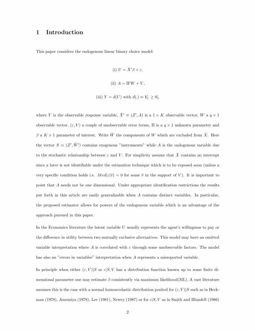
1 Introduction

This paper considers the endogenous linear binary choice model:

(i) U = X ′β + ε,

(ii) A = Π′W + V ,

(iii) Y = d(U) with d(.) ≡ 1[. ≥ 0],

where Y is the observable response variable, X ′ ≡ (Z ′, A) is a 1 × K observable vector, W a q × 1

observable vector, (ε, V ) a couple of unobservable error terms, Π is a q × 1 unknown parameter and

β a K × 1 parameter of interest. Write W the components of W which are excluded from X. Here

the vector S ≡ (Z ′, W ′) contains exogenous ”instruments” while A is the endogenous variable due

to the stochastic relationship between ε and V . For simplicity assume that X contains no intercept

since a later is not identifiable under the estimation technique which is to be exposed soon (unless a

very specific condition holds i.e. Med(ε|v) = 0 for some v in the support of V ). It is important to

point that A needs not be one dimensional. Under appropriate identification restrictions the results

put forth in this article are easily generalizable when A contains distinct variables. In particular,

the proposed estimator allows for powers of the endogenous variable which is an advantage of the

approach pursued in this paper.

In the Economics literature the latent variable U usually represents the agent’s willingness to pay or

the difference in utility between two mutually exclusive alternatives. This model may have an omitted

variable interpretation where A is correlated with ε through some unobservable factors. The model

has also an ”errors in variables” interpretation when A represents a misreported variable.

In principle when either (ε, V )|S or ε|S, V has a distribution function known up to some finite di-

mensional parameter one may estimate β consistently via maximum likelihood(ML). A vast literature

assumes this is the case with a normal homoscedastic distribution posited for (ε, V )|S such as in Heck-

man (1978), Amemiya (1978), Lee (1981), Newey (1987) or for ε|S, V as in Smith and Blundell (1986)

2

and Rivers and Vuong (1988). If the parametrization of the distribution in question is incorrect those

estimators will be inconsistent. Since an assumption involving the parametrization of the distribution

of ε is not testable per see (Newey 1985, Pagan and Vella 1989), new ”semi parametric” estimators

have been proposed relaxing this parametric requirement. For instance, the quasi ML estimator pro-

posed in Rothe (2009) is consistent for β whenever the distribution function of ε|X, V depends only

on X ′β and V . Also, the two stage least square estimator developed in Lewbel (2000) is consistent

for β provided there exists a ”special regressor” in X meeting a certain conditional independence

restriction. Even though these semi parametric estimators offer a robust advantage, they present

some limitations in terms of either the permitted form of heteroscedasticity (Rothe 2009) or which

variables affect the scedasticity of both ε and V (Lewbel 2000). This is due to the very nature of their

distributional oriented assumptions.

Estimators that are robust to unknown heteroscedasticity are based instead on some conditional

median restrictions which loosely speaking only require the center of the distribution of ε to re-

main unaffected by the covariates. For instance, Newey (1985) provided a consistent asymptotically

normally distributed two stage maximum score estimator for β under the requirement that (V, ε) be

symmetrically distributed around the origin conditional on S. Also, Hong and Tamer (2003) proposed

a consistent minimum distance estimator for β under the less restrictive condition that Med(ε|S) = 0

almost surely (a.s.). However, in Newey (1985) a consistent estimator for the asymptotic covariance is

not provided (see Newey 1985, page 228) while Hong and Tamer’s estimator has an unknown limiting

distribution.

The main motivation behind this article is to remedy this inferential problem offering a consistent

estimator of β which only imposes a weak median restriction but does allow for testing. The main es-

timator presented in this article, named the ”Kernel Weighted Smoothed Maximum Score” (KWSMS)

estimator, meets these objectives. The KWSMS estimator is constructed by imposing a restriction on

Med(ε|S, V ) which must not vary with the instruments. This ensures the existence of some random

variable φ and unobservable term e such that Y = d(X ′β + φ + e) where now e satisfies the clas-

sic median restriction introduced for Maximum Score estimation (Manski 1985). Then, a smoothed

3

Maximum Score estimation (Horowitz 1992) is performed as if φ were a constant correcting this ap-

proximation by means of a kernel. Doing so facilitates the asymptotic analysis using the framework

laid out in Horowitz 1992. An interesting additional contribution of this article is in fact to offer a

robust estimation procedure for a semi linear random utility model.

Not surprisingly, this estimation approach imposes stronger assumptions than those required from the

SMSE albeit similar in essence. The KWSMS estimator’s consistency for β (up to a positive scale)

requires that one element of X be fully supported and that the endogenous variable be continuous.

Additionally, if certain cumulative distribution functions involving the random variables V and X ′β are

sufficiently differentiable then the KWSMS estimator is asymptotically normally distributed provided

the fourth moments of X exist. Finally, the discrepancy between the KWSMS estimator and β is

Op(n− 1

2 +ε) for some chosen ε ∈ (κ, 1/8) where κ is a positive constant becoming arbitrary small under

adequate regularity conditions. Hence, the parametric rate is potentially achievable.

This paper relates to the previous literatures using the control function approach which has already

been employed to handle endogeneity in the context of binary choice models (Blundell and Powell

2004), triangular equation models (Newey, Powell and Vella 1999) and quantile regression models (Lee

2007). Also, the technique used to derive the asymptotic results is similar to that of the SMSE using

non parametric convolution based arguments. Finally, its local nature can be thought as a smoothed

analogue of the local quantile regression estimator (Chaudhuri 1991, Lee 2003) in the context of the

random utility model.

As explained in section 2.2, a KWSMS estimator in effect uses only observations of V close to a

given value. This local nature suggests that the rate of convergence can be accelerated by using more

observations of V instead. Thus, in this paper a second stage estimation is offered with a ”Score

Approximation Smoothed Maximum Score” (SASMS) estimator which uses the information content

from various KWSMS estimators retrieved in a first stage estimation. Under stronger regularity

conditions the SASMS estimator is still consistent and asymptotically normally distributed while

achieving a faster rate of convergence. Additionally, the SASMS estimator is a plug-in estimator

which does not require solving a non linear optimization problem once the first stage estimation is

4

completed.

The rest of the paper is organized as follows. Section 2 provides a rapid review of the control func-

tion approach in the context of this binary choice model and defines the KWSMS estimator. Section

3 presents some sufficient conditions for identification. Section 4 covers the KWSMS estimator’s

asymptotic properties. Section 5 gives some generic assumptions for the SASMS estimator’s asymp-

totic properties. Finally, section 6 exhibits some Monte Carlo simulations to illustrate the finite sample

qualities of the suggested estimators. All the proofs are to be found in the appendix.

At this point, it is convenient to introduce some notations used throughout the subsequent sections:

(1)For f:R −→ R define f (j)(t) its jth derivative at t whenever this later exists. Also, when the

function is defined everywhere use ||f ||sup ≡ supt∈R|f(t)|.

(2) The triplet (Ω,=, P ) refers to a probability space where Ω is the space of states of nature, = is

the sigma field of measurable events and P the probability measure.

(3)For a joint couple of real valued random variables (A,B) define fb(a) as the Lebesgue density of A

conditional on B = b whenever this later exists and FA|B(.) = P [A ≤ .|B]. When T is a measurable

random variable of dimension say |T |, a property will be said to be met ”a.e in t” if that the property

is true except maybe when t ∈ N with P [T ∈ N] = 0 and N is some real Borel set of R|T |.

(4)For s ∈ N∗, define Ks=f : R −→ R , f Borel, ||f ||sup < ∞,∫f(t)dt = 1,

∫tuf(t)dt = 0

for u = 1, ..., s − 1 and∫|tuf(t)|dt < ∞ for u = 0, s. Also, given a positive number M, define

Cs∞(M)=f : R −→ R, f (j) exists and is continuous for j = 0, 1, ..., s everywhere with |f (j)| < M

for j = 0, 1, ..., s, and given a real number t define Cs∞(t,M)=f : R −→ R, f exists everywhere

with |f | < M and there exists an open neighborhood of t on which f (j) exists, is continuous with

|f (j)| < M for j = 1, ..., s.

(5) Given a strictly positive deterministic sequence ann≥1 and a deterministic sequence cnn≥1 the

notation cn = o(an) is used if lim cn/an = 0 as n → ∞. The notation cn = O(an) is used if cn/an

is a bounded sequence. When cnn≥1 is a sequence of measurable random variables defined on some

probability space (Ω,=, P ) the convention cn = op(an) is employed if for any ε > 0 there exists a

5

natural number N such that n ≥ N implies P [|cn/an| > ε] < ε. Finally, cn = Op(an) is used if for

any ε > 0 there exists a positive number M < ∞ and natural number N such that n ≥ N implies

P [|cn/an| > M ] < ε.

2 Informal Summary of the KWSMS Estimator

Section 2.1 provides an intuitive account of the control function approach in the context of the binary

model presented above which is instructive to understand the essence of the estimation strategy

pursued in this article. Section 2.2 offers an informal description of the KWSMS estimator.

2.1. Estimation Strategy

The key condition introduced in this paper is that there exists some v in the support of V satisfying:

[1] Med(ε|Z,W, V = v) = Med(ε|V = v) a.s.,

Loosely speaking, [1] imposes that once V has been fixed at v, the exogenous variables becomes

uninformative to alter the center of the distribution of ε. This holds for instance when (Z,W ) ⊥ (ε, V )

or under a ”global” restriction Fε|Z,W,V ≡ Fε|V a.s. but those are not necessary. This key median

assumption, which can be tested from data as given in section C of the Appendix, is neither stronger

nor weaker than that assumed in Hong and Tamer (2003) because each restriction can be implied by

the other under certain conditions. This median restriction can accommodate heteroscedasticity in V

of unknown form in the error term. However, in some cases heteroscedasticity in some variables of X

let’s say Xs only permits a more general restriction Med(ε|Z,W, V ) = Med(ε|Xs, V ) a.s. violating

[1]. Fortunately, the methodology developed in this paper can be extended to identify and estimate

the coefficients of the variables ”purged” by the control as explained in section A of the appendix.

Let suppose now that [1] holds for almost every arbitrary v. As will be explained shortly, this is

stronger than required for the KWSMS estimator but is needed for the SASMS estimator (at least

over a range of values for v). Invoking this last condition and the fact (X, V ) is one to one with

(Z,Π′W,V ) yields:

6

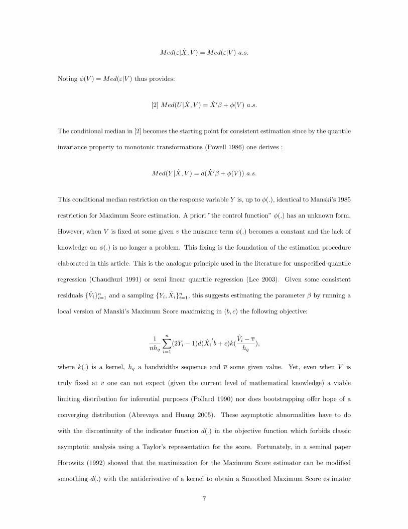
Med(ε|X, V ) = Med(ε|V ) a.s.

Noting φ(V ) = Med(ε|V ) thus provides:

[2] Med(U |X, V ) = X ′β + φ(V ) a.s.

The conditional median in [2] becomes the starting point for consistent estimation since by the quantile

invariance property to monotonic transformations (Powell 1986) one derives :

Med(Y |X, V ) = d(X ′β + φ(V )) a.s.

This conditional median restriction on the response variable Y is, up to φ(.), identical to Manski’s 1985

restriction for Maximum Score estimation. A priori ”the control function” φ(.) has an unknown form.

However, when V is fixed at some given v the nuisance term φ(.) becomes a constant and the lack of

knowledge on φ(.) is no longer a problem. This fixing is the foundation of the estimation procedure

elaborated in this article. This is the analogue principle used in the literature for unspecified quantile

regression (Chaudhuri 1991) or semi linear quantile regression (Lee 2003). Given some consistent

residuals Vini=1 and a sampling Yi, Xini=1, this suggests estimating the parameter β by running a

local version of Manski’s Maximum Score maximizing in (b, c) the following objective:

1

nhq

n∑i=1

(2Yi − 1)d(Xi′b+ c)k(

Vi − vhq

),

where k(.) is a kernel, hq a bandwidths sequence and v some given value. Yet, even when V is

truly fixed at v one can not expect (given the current level of mathematical knowledge) a viable

limiting distribution for inferential purposes (Pollard 1990) nor does bootstrapping offer hope of a

converging distribution (Abrevaya and Huang 2005). These asymptotic abnormalities have to do

with the discontinuity of the indicator function d(.) in the objective function which forbids classic

asymptotic analysis using a Taylor’s representation for the score. Fortunately, in a seminal paper

Horowitz (1992) showed that the maximization for the Maximum Score estimator can be modified

smoothing d(.) with the antiderivative of a kernel to obtain a Smoothed Maximum Score estimator

7

which permits to get back into this classic asymptotic framework whenever the kernel in question is

smooth. This suggests constructing a consistent and asymptotically normally distributed estimator

by using a smoothed version of the above objective. This is the estimation’s path adopted in this

paper.

This differs from the previous Control Function literature (Newey, Powell and Vella 1999) and (Lee

2007) where the control function is not fixed but rather expanded via Sieves. However, the specific

problem here is different because of the indicator variable in the objective and using the conven-

tional approach would involve stronger assumptions for both identification purposes and asymptotic

purposes.

2.2. Description of the KWSMS Estimator

Define the parameters Πw and Πz from Π′W = Π′wW + Π′zZ where W contains exogenous variables

excluded from Z.

The parameter of interest β is only identifiable up to a positive scale since d(cU) = d(U) for any c > 0.

Identification up to a positive scale requires three main conditions. First, the distribution function of

V |X needs to admit a density with respect to the Lebesgue measure which exists at the chosen v (a.s.).

Consequently, another prerequisite for identification up to scale is a ”rank condition” demanding W to

contain one component which is not a function of Z and whose associated slope coefficient is non null.

To understand this recall that X ′ ≡ (Z ′, A) so that V = A − Π′W becomes a deterministic function

of X should the last mentioned ”rank condition” fail making V |X a single atom with a degenerated

Dirac distribution. Finally, one element of X conditional on its remaining elements must possess a

distribution function absolutely continuous with respect to the Lebesgue measure (a.s.). Let (C, X ′)

be a partition of X ′ such that the scalar variable C satisfies this property and write β1 its associated

slope coefficient. These conditions combined with [1] and some conventional regularity conditions

suffice for identification up to the scaling factor 1/|β1| whenever β1 6= 0. Thus, assume without loss

of generality that β1 is known to be strictly positive.1

1All the asymptotic results can be conducted using the fact that the estimator of β1|β1|∈ −1, 1 is equal to β1

|β1|with

8

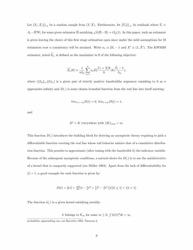
Let Yi, Xini=1 be a random sample from (Y, X). Furthermore, let Vini=1 be residuals where Vi ≡

Ai− Π′Wi for some given estimator Π satisfying√n(Π−Π) = Op(1). In this paper, such an estimator

is given leaving the choice of this first stage estimation open since under the mild assumptions for M

estimators root n consistency will be attained. Write αi ≡ 2Yi − 1 and X ′ ≡ (1, X ′). The KWSMS

estimator, noted θn, is defined as the maximizer in θ of the following objective:

Sn(θ) ≡ 1

nhq

n∑i=1

αiD(Ci +X ′iθ

h)k(

Vi − vhq

),

where (hqn,hn) is a given pair of strictly positive bandwidths sequences vanishing to 0 as n

approaches infinity and D(.) is some chosen bounded function from the real line into itself meeting:

limt→−∞D(t) = 0, limt→∞D(t) = 1,

and

D′ = K everywhere with ||K||sup <∞.

This function D(.) introduces the building block for deriving an asymptotic theory requiring to pick a

differentiable function covering the real line whose tail behavior mimics that of a cumulative distribu-

tion function. This permits to approximate (after tuning with the bandwidth h) the indicator variable.

Because of the subsequent asymptotic conditions, a natural choice for D(.) is to use the antiderivative

of a kernel that is compactly supported (see Muller 1984). Apart from the lack of differentiability for

|t| = 1, a good example for such function is given by:

D(t) = [0.5 + 10564 (t− 5

3 t3 + 7

5 t5 − 3

7 t7)]1[|t| ≤ 1] + 1[t > 1].

The function k(.) is a given kernel satisfying notably:

k belongs to Km for some m ≥ 2,∫|k(t)|2dt <∞,

probability approaching one, see Horowitz 1992, Theorem 2.

9

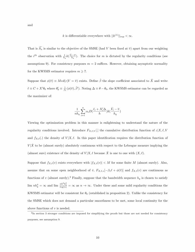
and

k is differentiable everywhere with ||k(1)||sup <∞.

That is Sn is similar to the objective of the SMSE (had V been fixed at v) apart from our weighting

the ith observation with 1hqk( Vi−vhq

). The choice for m is dictated by the regularity conditions (see

assumptions 9). For consistency purposes m = 2 suffices. However, obtaining asymptotic normality

for the KWSMS estimator requires m ≥ 7.

Suppose that φ(v) ≡ Med(ε|V = v) exists. Define β the slope coefficient associated to X and write

` ≡ C +X ′θ0 where θ′0 ≡ 1β1

(φ(v), β′). Noting ∆ ≡ θ− θ0, the KWSMS estimator can be regarded as

the maximizer of:

1

nhq

n∑i=1

αiD(`i +X ′i∆

h)k(

Vi − vhq

)

Viewing the optimization problem in this manner is enlightening to understand the nature of the

regularity conditions involved. Introduce FX,`,V [.] the cumulative distribution function of ε|X, `, V

and fX,`(.) the density of V |X, `. In this paper identification requires the distribution function of

V |X to be (almost surely) absolutely continuous with respect to the Lebesgue measure implying the

(almost sure) existence of the density of V |X, ` because X is one to one with (X, `).

Suppose that fX,`(v) exists everywhere with |fX,`(v)| < M for some finite M (almost surely). Also,

assume that on some open neighborhood of v, FX,`,v[−β1` + φ(v)] and fX,`(v) are continuous as

functions of v (almost surely).2 Finally, suppose that the bandwidth sequence hq is chosen to satisfy

lim nh4q = ∞ and lim

nh2h2q

log(n) = ∞ as n → ∞. Under these and some mild regularity conditions the

KWSMS estimator will be consistent for θ0 (established in proposition 2). Unlike the consistency for

the SMSE which does not demand a particular smoothness to be met, some local continuity for the

above functions of v is needed.

2In section 3 stronger conditions are imposed for simplifying the proofs but those are not needed for consistency

purposes, see assumption 9.

10

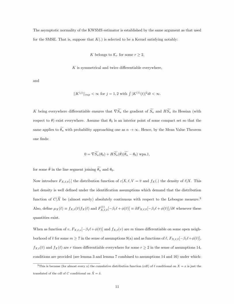
The asymptotic normality of the KWSMS estimator is established by the same argument as that used

for the SMSE. That is, suppose that K(.) is selected to be a Kernel satisfying notably:

K belongs to Kr for some r ≥ 2,

K is symmetrical and twice differentiable everywhere,

and

||K(j)||sup <∞ for j = 1, 2 with∫|K(1)(t)|2dt <∞.

K being everywhere differentiable ensures that ∇Sn the gradient of Sn and HSn its Hessian (with

respect to θ) exist everywhere. Assume that θ0 is an interior point of some compact set so that the

same applies to θn with probability approaching one as n→∞. Hence, by the Mean Value Theorem

one finds:

0 = ∇Sn(θ0) +HSn(θ)(θn − θ0) wpa.1,

for some θ in the line segment joining θn and θ0.

Now introduce FX,`,v[.] the distribution function of ε|X, `, V = v and fX(.) the density of `|X. This

last density is well defined under the identification assumptions which demand that the distribution

function of C|X be (almost surely) absolutely continuous with respect to the Lebesgue measure.3

Also, define µX(`) ≡ fX,`(v)fX(`) and F(1)X,`,v[−β1`+φ(v)] ≡ ∂FX,`,v[−β1`+φ(v)]/∂` whenever these

quantities exist.

When as function of v, FX,`,v[−β1`+φ(v)] and fX,`(v) are m times differentiable on some open neigh-

borhood of v for some m ≥ 7 in the sense of assumptions 9(a) and as functions of `, FX,`,v[−β1`+φ(v)],

fX,`(v) and fX(`) are r times differentiable everywhere for some r ≥ 2 in the sense of assumptions 14,

conditions are provided (see lemma 3 and lemma 7 combined to assumptions 14 and 16) under which:

3This is because (for almost every x) the cumulative distribution function (cdf) of ` conditional on X = x is just the

translated of the cdf of C conditional on X = x.

11

plim HSn(θ) ≡ H0,

where H0 ≡ 2E[XX ′F(1)X,0,v[φ(v)]µX(0)]. Let further suppose that H0 is negative definite. The

plausibility of this definiteness is discussed on page 18. Furthermore, if the bandwidths are selected

appropriately according to assumption 17 and if the kernels k and K satisfy some mild integrability

conditions one can further establish (see lemma 5 and lemma 8):

√nhhq∇Sn(θ0)→d N (0,Σ0),

where Σ0 ≡∫|k|2

∫|K|2E[XX ′µX(0)]. It will hence follow that:

[4]√nhhq(θn − θ0) →d N (0,ℵ),

where ℵ ≡ H−10 Σ0H

−10 can be estimated consistently from data as given in proposition 4.

As explained on page 19 the bandwidths can be selected according to the followings:

pick h ∝ n−a and hq ∝ n−aq where a and aq are some chosen constants satisfying:

a ∈ (Max 11+η+2ηm ; 1

1+η+2r,1

4+4η ), and

aq = ηa for some η ∈ ( 32m−3 ,

13 ).

The asymptotic result from [4] and the above bandwidths criteria imply that the KWSMS estimator,

under relatively weak smoothness conditions, satisfies at least θn−θ0 = Op(n−3/8). However, this rate

may improve when λ = Minm, r augments eventually reaching the parametric rate i.e. Op(n−1/2)

whenever λ approaches infinity.

The KWSMS estimator has an asymptotically centered normal distribution because the bandwidths

pair has been selected purposefully such that the asymptotic bias vanishes which translates here

into lim nh2m+1q h = 0 and lim nh2r+1hq = 0 as n → ∞. In the non parametric jargon ”under

smoothing” is employed. As established in Horowitz (1992) this is not optimal from an asymptotic

mean squared error perspective which requires some strictly positive finite bias. This choice is driven

12

by two considerations. First, the construction of an asymptotically biased KWSMS estimator would

impose additional regularity conditions. Secondly, the unbiased SMSE has superior bootstrapping

properties than the biased SMSE (see Horowitz 2002) in terms of the accuracy of its bootstrapped

critical values which suggests the analogue for the KWSMS estimator since the objective of the

KWSMS estimator is just a weighted version of SMSE’s objective.

It is worth pointing a practical concern. The maximization of the objective function will be carried out

by an iterative procedure such as the quadratic hill climbing (Goldfeld, Quandt and Trotter 1966).

Additionally, the starting value for the iterative search may be better chosen as a result of some

annealing procedure (see Horowitz 1992 and Szu et al. 1987).

3 Identification

The identification of β (up to a positive scale) is ensured under the followings:

Assumption 1:

W has one component which is not measurable4in Z and whose associated slope coefficient is non null.

Assumption 2:

There exists a partition of X ′ = (C, X ′) where dim C =1 and such that its corresponding slope

coefficient, noted β1, is strictly positive.

Assumption 3:

(a) There exists some given v ∈ R and some φ(v) ∈ R such that:

P [ε ≤ φ(v)|Z = z,W = w, V = v] = 12 a.e.in z,w.

(b) The distribution function of ε|X = x, V = v has everywhere positive density with respect to the

Lebesgue measure a.e.in x.

4A random variable is said to be measurable in Z if it has the form f(Z) for some Borel function f . The function is

Borel if for any real number a the preset f−1(a,∞) is a Borel set. Most functions of Z encountered in applied work are

measurable in Z such as powers of Z, intercept, the indicator involving the level of Z and the conditional mean E[T |Z]

provided E|T | <∞.

13

Assumption 4 :

(a) The distribution function of C|X = x has everywhere positive density with respect to the Lebesgue

measure a.e.in x.

(b) The distribution function of V |X = x is absolutely continuous with respect to the Lebesgue measure

a.e.in x and its density evaluated at v exists a.e.in x. Furthermore, there exists some real number

Mv <∞ such that 0 < f(v|x) < Mv a.e.in x.

Assumption 5:

E[XX ′] is positive definite where X ′ ≡ (1, X ′).

Comments: Assumption 1 is a rank condition requiring at least one excluded instrument which is

not a function of Z having an impact on the endogenous variable (see Lee 2007 and Newey, Powell and

Vella 1999). Consider for instance the simple case where Z is a scalar variable and W = (Z,Z2). Even

though Z2 is not part of X assumption 1 fails. More generally, adding functions of the exogenous

variables including in (i) to the reduced form equation (ii) is not a viable strategy in the context of our

estimation problem. Assumptions 2 demands one variable whose marginal impact on the latent index

X ′β is positive. As pointing out earlier merely β1 non null suffices because our parameter of interest

is estimated up to the constant 1|β1| and all of our results can be generalized by adding β1

|β1| ∈ −1, 1

as an additional unknown parameter. Assumption 3(a) is a classic control function condition except

that only a local restriction at some v is imposed. Assumption 3(b), introduced similarly to Manski’s

1985 assumption 2b, prevents the binary outcome Y from being perfectly predictable by (X,v) with

some strictly positive probability.5 Assumption 4 contains classic slack conditions permitting LMDR-

identification (see Manski 1985, lemma 2) in the context of our control function approach. This is

a prerequisite to identification which requires the existence of a significant (in the sense of having a

coefficient non null) variable in X that must be fully supported. The additional presence of V in the

controlled model imposes that V |X be supported on some neighborhood (albeit small) of v. Finally,

assumption 5 prevents identification of an intercept in X.

5Assumption 3(b) is equivalent to P [Y = 1|X = x, V = v] ∈ (0, 1) a.e. in x.

14

Now write φ(v) ≡Med(ε|V = v) and θ′0 ≡ 1β1

(φ(v), β′) where β denotes the slope coefficient associated

to X.

Proposition 1 (Identification)

Under assumptions 1 through 5,

θ0 ≡ Argmaxθ∈RKE[d(`+X ′(θ − θ0))gX,`(v)],

where ` ≡ C + X ′θ0, gX,`(v) ≡ (1 − 2FX,`,v[−β1` + φ(v)])fX,`(v), FX,`,v[.] indicates the cumulative

distribution function of ε|X, `, V = v and fX,`(v) indicates the density of V |X, ` evaluated at v.

4 Asymptotic Properties of the KWSMS Estimator

Let Yi, Xini=1 be a sequence of observations and let Π be some given estimator from a first stage

estimation inducing Vi ≡ Ai−Π′Wi for i = 1...n. Also, let hq and h be two strictly positive bandwidths

sequences, D(.) some given function from the real line into itself and k(.) a kernel. For any θ ∈ RK

define the following objective:

Sn(θ) =1

nhq

n∑i=1

αiD(Ci +X ′iθ

h)k(

Vi − vhq

).

Sufficient conditions for weak consistency are given next.

Assumption 6:

Yi, Xi,Wini=1 is an iid sequence from (Y, X,W ) satisfying Y = d(X ′β + ε).

Assumption 7:

The support of W is a bounded subset of Rq with q ≥ 1.

Assumption 8:

θ0 is an interior point of Θ ⊂ RK compact.

15

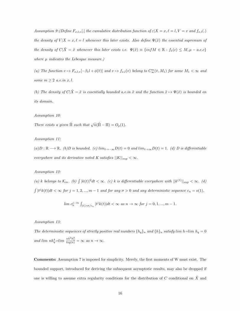
Assumption 9 :(Define Fx,l,v[.] the cumulative distribution function of ε|X = x, ` = l, V = v and fx,l(.)

the density of V |X = x, ` = l whenever this later exists. Also define Ψ(x) the essential supremum of

the density of C|X = x whenever this later exists i.e. Ψ(x) ≡ infM ∈ R : fx(c) ≤ M,µ − a.e.c

where µ indicates the Lebesgue measure.)

(a) The function v 7→ Fx,l,v[−β1l+φ(v)] and v 7→ fx,l(v) belong to Cm∞(v,M1) for some M1 <∞ and

some m ≥ 2 a.e.in x, l.

(b) The density of C|X = x is essentially bounded a.e.in x and the function x 7→ Ψ(x) is bounded on

its domain.

Assumption 10:

There exists a given Π such that√n(Π−Π) = Op(1).

Assumption 11:

(a)D : R −→ R. (b)D is bounded. (c) limt→−∞D(t) = 0 and limt→∞D(t) = 1. (d) D is differentiable

everywhere and its derivative noted K satisfies ||K||sup <∞.

Assumption 12:

(a) k belongs to Km. (b)∫|k(t)|2dt <∞. (c) k is differentiable everywhere with ||k(1)||sup <∞. (d)∫

|tjk(t)|dt <∞ for j = 1, 2, ...,m− 1 and for any σ > 0 and any deterministic sequence cn = o(1),

lim cj−mn

∫|t|>σ/cn |t

jk(t)|dt <∞ as n→∞ for j = 0, 1, ...,m− 1.

Assumption 13:

The deterministic sequences of strictly positive real numbers hqn and hn satisfy lim h=lim hq = 0

and lim nh4q=lim

nh2h2q

log(n) =∞ as n→∞.

Comments: Assumption 7 is imposed for simplicity. Merely, the first moments of W must exist. The

bounded support, introduced for deriving the subsequent asymptotic results, may also be dropped if

one is willing to assume extra regularity conditions for the distribution of C conditional on X and

16

W . Assumption 8 is technical identically to assumption 4 in Horowitz (1992) because proposition 1

covers RK while consistency is easier to establish for a compact set. Assumption 9(a) will be met for

instance when both Fε|x,v and fx(v) as functions of v are twice continuously differentiable on some

open neighborhood of the chosen v with some bound on the first and second derivatives (a.e.in x).

Assumption 9(b) is technical but is needed to get a uniform convergence for the empirical moment Sn.

Assumption 10 is verified under the mild assumptions for M estimators. Assumption 11 introduces

the building block for smoothing the indicator function. As explained in the introduction, an easy

manner to construct such a function is by integrating a kernel but for consistency purposes this is not

needed. Assumption 12 is for the most part a typical condition which demands to select the order of

the kernel k(.) to match the smoothness of the function it will convolute with.

Proposition 2 (KWSMS Consistency)

Under the assumptions of proposition 1 and assumptions 6 through 13,

θn ≡ ArgmaxΘSn(θ) is (weakly) consistent for θ0.

To derive a normal limiting distribution for the estimator introduce the following conditions:

Assumption 14:(Define gx,l(v) ≡ (1−2Fx,l,v[−β1l+φ(v)])fx,l(v) where Fx,l,v[.] indicates the cumulative

distribution function of ε|X = x, ` = l, V = v and fx(.) the density of `|X = x whenever this later

exists.). The function l 7→ gx,l(v) and l 7→ fx(l) belong to Cr∞(M2) for some M2 <∞ and some r ≥ 2

a.e.in x.

Assumption 15:

(a)E||X||4 <∞.

(b)E[XX ′T(1)X (0)] is positive definite where TX(l) ≡ gX,l(v)fX(l) and T

(1)X (u) ≡ ∂TX

∂l |l=u.

Assumption 16:

(a)K belongs to Kr and is symmetrical.

17

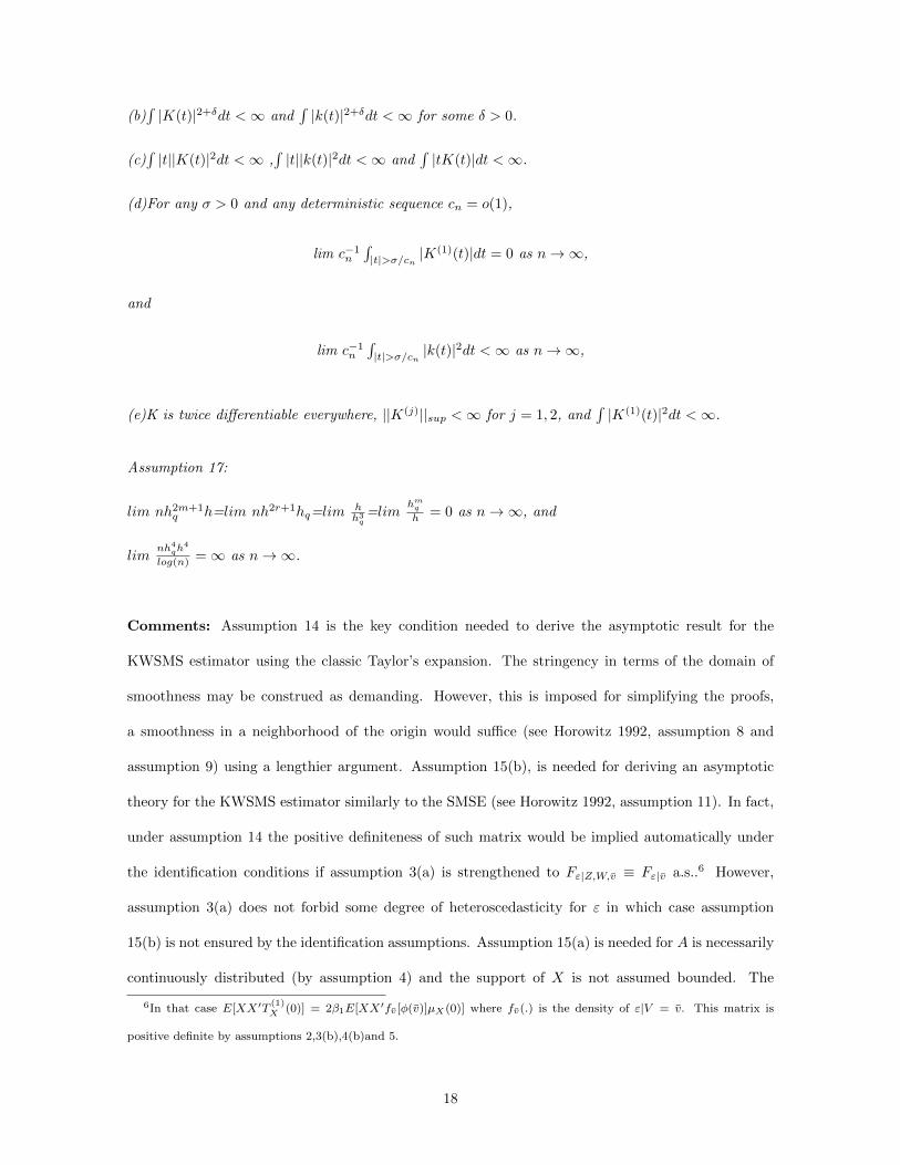
(b)∫|K(t)|2+δdt <∞ and

∫|k(t)|2+δdt <∞ for some δ > 0.

(c)∫|t||K(t)|2dt <∞ ,

∫|t||k(t)|2dt <∞ and

∫|tK(t)|dt <∞.

(d)For any σ > 0 and any deterministic sequence cn = o(1),

lim c−1n

∫|t|>σ/cn |K

(1)(t)|dt = 0 as n→∞,

and

lim c−1n

∫|t|>σ/cn |k(t)|2dt <∞ as n→∞,

(e)K is twice differentiable everywhere, ||K(j)||sup <∞ for j = 1, 2, and∫|K(1)(t)|2dt <∞.

Assumption 17:

lim nh2m+1q h=lim nh2r+1hq=lim

hh3q

=limhmqh = 0 as n→∞, and

limnh4

qh4

log(n) =∞ as n→∞.

Comments: Assumption 14 is the key condition needed to derive the asymptotic result for the

KWSMS estimator using the classic Taylor’s expansion. The stringency in terms of the domain of

smoothness may be construed as demanding. However, this is imposed for simplifying the proofs,

a smoothness in a neighborhood of the origin would suffice (see Horowitz 1992, assumption 8 and

assumption 9) using a lengthier argument. Assumption 15(b), is needed for deriving an asymptotic

theory for the KWSMS estimator similarly to the SMSE (see Horowitz 1992, assumption 11). In fact,

under assumption 14 the positive definiteness of such matrix would be implied automatically under

the identification conditions if assumption 3(a) is strengthened to Fε|Z,W,v ≡ Fε|v a.s..6 However,

assumption 3(a) does not forbid some degree of heteroscedasticity for ε in which case assumption

15(b) is not ensured by the identification assumptions. Assumption 15(a) is needed for A is necessarily

continuously distributed (by assumption 4) and the support of X is not assumed bounded. The

6In that case E[XX′T(1)X (0)] = 2β1E[XX′fv [φ(v)]µX(0)] where fv(.) is the density of ε|V = v. This matrix is

positive definite by assumptions 2,3(b),4(b)and 5.

18

existence of the fourth moment permits some control to show the convergence of certain expected

values notably the collapse of the limiting bias. Assumption 16(a) is a reflection of assumption 14

since various convolutions involving K(.) need to converge in some senses. Assumptions 16(b) and

16(c) are stability conditions for obtaining asymptotic Normality and are satisfied by many kernels, a

clear example of which being polynomials compactly supported kernels which are smooth at boundary

points. Finally, assumptions 16(d) and 16(e) are needed for the Hessian to converge in probability

to some finite quantity and is related to assumptions 7 of Horowitz (1992), which demands the first

two derivatives of K(.) to be well behaved. Finally, assumption 17 dictates the bandwidths’ rate

which must be selected for the asymptotic to be met with lim nh2m+1q h=lim nh2r+1hq=0 collapsing

the asymptotic bias while lim hh3q=0 allows the usage of the estimated nuisance V (A,W ) via Π to be

asymptotically irrelevant.

Proposition 3 (KWSMS Asymptotic Normality)

Under the assumptions of proposition 2 and assumptions 14 through 17,

√nhhq(θn − θ0) →d N (0, H−1ΣH−1),

where

H ≡ E[XX ′T(1)X (0)], Σ ≡

∫|k|2

∫|K|2E[XX ′µX(0)] and µX(`) ≡ fX,`(v)fX(`).

Comments: So far it is implicitly assumed that both assumptions 13 and 17 are met. However,

this imposes some smoothness conditions beyond those assumed in assumptions 9. When h ∝ n−a

and hq ∝ n−aq for some strictly positive constants a and aq, the bandwidths requirement put forth

in proposition 3 will hold as long as a ∈ (Max 11+η+2ηm ; 1

1+η+2r,1

4+4η ) and aq = ηa for some

η ∈ ( 32m−3 ,

13 ).7 Thus, the asymptotic conclusion needs a strengthening to m ≥ 7 in assumption 9.

Under this last condition and r ≥ 2, one can therefore obtain a rate on convergence in probability

7It is clear that Assumptions 13 and 17 both hold as long as lim nh2m+1q h=lim nh2r+1hq=0 , lim h

h3q

=limhmqh

=0

and limnh4qh

4

log(n)=∞. Solving these implied inequalities directly yields the bandwidths spectrum given above.

19

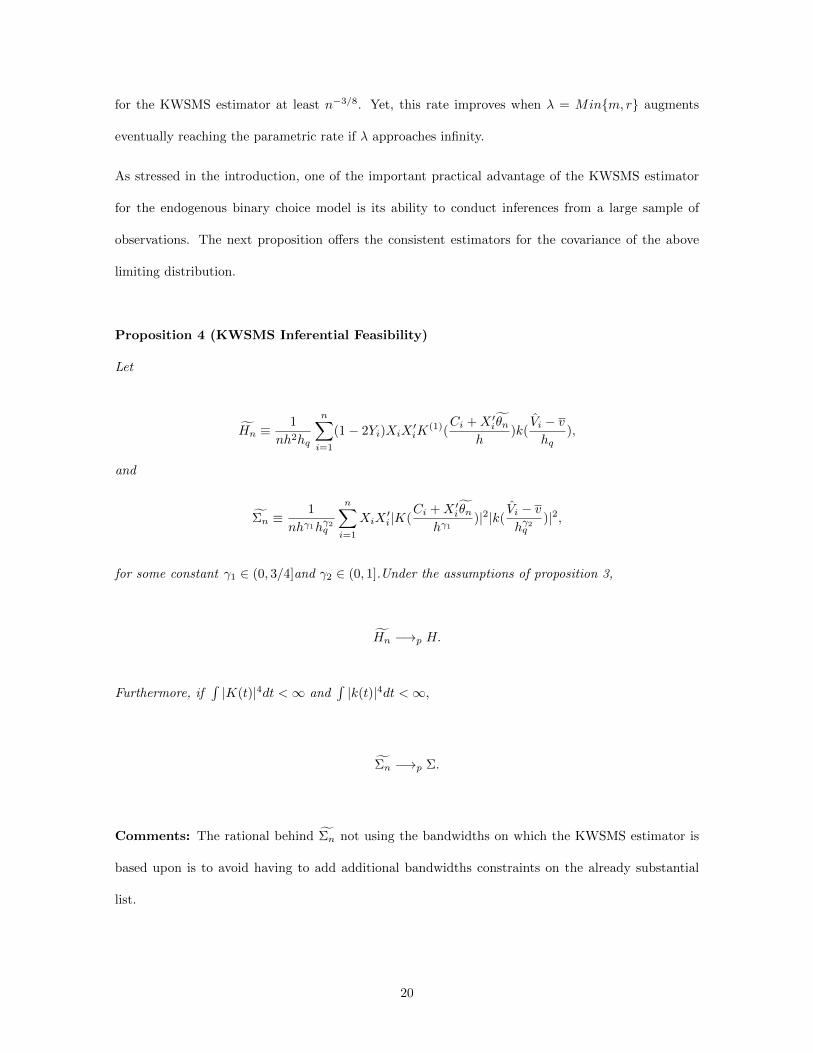
for the KWSMS estimator at least n−3/8. Yet, this rate improves when λ = Minm, r augments

eventually reaching the parametric rate if λ approaches infinity.

As stressed in the introduction, one of the important practical advantage of the KWSMS estimator

for the endogenous binary choice model is its ability to conduct inferences from a large sample of

observations. The next proposition offers the consistent estimators for the covariance of the above

limiting distribution.

Proposition 4 (KWSMS Inferential Feasibility)

Let

Hn ≡1

nh2hq

n∑i=1

(1− 2Yi)XiX′iK

(1)(Ci +X ′i θn

h)k(

Vi − vhq

),

and

Σn ≡1

nhγ1hγ2q

n∑i=1

XiX′i|K(

Ci +X ′i θnhγ1

)|2|k(Vi − vhγ2q

)|2,

for some constant γ1 ∈ (0, 3/4]and γ2 ∈ (0, 1].Under the assumptions of proposition 3,

Hn −→p H.

Furthermore, if∫|K(t)|4dt <∞ and

∫|k(t)|4dt <∞,

Σn −→p Σ.

Comments: The rational behind Σn not using the bandwidths on which the KWSMS estimator is

based upon is to avoid having to add additional bandwidths constraints on the already substantial

list.

20

5 Accelerating Convergence with a Score Approximation Smoothed

Maximum Score Estimator

As explained in the previous section, a KWSMS estimator’s rate of convergence will be as rapid

as the order of differentiability of certain cumulative distribution functions and densities. Under

low differentiability one may thus seek to construct an alternative estimator with a faster rate of

convergence in probability by using more observations of V . In this section, the SASMS estimator

is shown to attain that target provided some stronger assumptions hold. In section 5.1 an informal

description of the SASMS estimator is presented. In section 5.2 the asymptotic’s properties of a

SASMS estimator are covered.

5.1. Description of the SASMS Estimator

In this section we present an informal description for constructing the SASMS estimator. Suppose

now that [1] holds for an arbitrary v ∈ [0, 1] which will be simply noted from now on v. Define

e′K ≡ [O, IK−1] the K − 1×K matrix where the first column is the zero vector while IK−1 represents

the K − 1×K − 1 identity matrix and e′1 the 1×K vector whose first entry is 1 and zero elsewhere.

Let Θ ⊂ RK be some given compact set and for a given v introduce the followings:

θ(v) ≡ ArgmaxΘ1

nhq

n∑i=1

αiD(Ci +X ′iθ

h)k(

Vi − vhq

),

and

β(v) ≡ e′K θ(v) while φ(v) ≡ e′1θ(v),

where D(.), k(.) and the bandwidths pair (h, hq) are as described in section 4. Let fjj≥1 be a known

basis of functions such that∑ρj=1 bjfj can approximate a smooth function of [0, 1] arbitrary well using

some real sequence bjj≥1 and natural number ρ large enough. There are many candidates for such

basis depending on the assumed topology of the smooth function involved. Classic examples include

power series, splines, trigonometric series and wavelets. Here are some easy to implement basis taken

from Chen (2007):

21

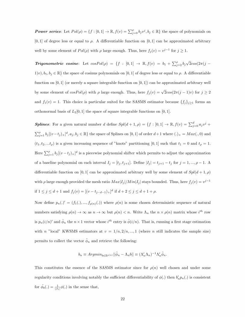
Power series: Let Pol(ρ) = f : [0, 1]→ R, f(v) =∑ρj=0 bjv

j , bj ∈ R the space of polynomials on

[0, 1] of degree less or equal to ρ. A differentiable function on [0, 1] can be approximated arbitrary

well by some element of Pol(ρ) with ρ large enough. Thus, here fj(v) = vj−1 for j ≥ 1.

Trigonometric cosine : Let cosPol(ρ) = f : [0, 1] → R, f(v) = b1 +∑ρj=2 bj

√2cos(2π(j −

1)v), b1, bj ∈ R the space of cosinus polynomials on [0, 1] of degree less or equal to ρ. A differentiable

function on [0, 1] (or merely a square integrable function on [0, 1]) can be approximated arbitrary well

by some element of cosPol(ρ) with ρ large enough. Thus, here fj(v) =√

2cos(2π(j − 1)v) for j ≥ 2

and f1(v) = 1. This choice is particular suited for the SASMS estimator because fjj≥1 forms an

orthonormal basis of L2[0, 1] the space of square integrable functions on [0, 1].

Splines: For a given natural number d define Spl(d + 1, ρ) = f : [0, 1] → R, f(v) =∑dj=0 ajv

j +∑ρj=1 bj [(v− tj)+]d, aj , bj ∈ R the space of Splines on [0, 1] of order d+1 where (.)+ = Max(., 0) and

(t1, t2, ...tρ) is a given increasing sequence of ”knots” partitioning [0, 1] such that t1 = 0 and tρ = 1.

Here∑ρj=1 bj [(v− tj)+]d is a piecewise polynomial shifter which permits to adjust the approximation

of a baseline polynomial on each interval Ij = [tj , tj+1]. Define |Ij | = tj+1 − tj for j = 1, ..., ρ− 1. A

differentiable function on [0, 1] can be approximated arbitrary well by some element of Spl(d + 1, ρ)

with ρ large enough provided the mesh ratio Max|Ij |/Min|Ij | stays bounded. Thus, here fj(v) = vj−1

if 1 ≤ j ≤ d+ 1 and fj(v) = [(v − tj−d−1)+]d if d+ 2 ≤ j ≤ d+ 1 + ρ.

Now define pn(.)′ = (f1(.), ..., fρ(n)(.)) where ρ(n) is some chosen deterministic sequence of natural

numbers satisfying ρ(n)→∞ as n→∞ but ρ(n) < n. Write Λn the n× ρ(n) matrix whose ith row

is pn(i/n)′ and φn the n× 1 vector whose ith entry is φ(i/n). That is, running a first stage estimation

with n ”local” KWSMS estimators at v = 1/n, 2/n, ..., 1 (where n still indicates the sample size)

permits to collect the vector φn and retrieve the following:

bn ≡ Argminb∈Rρ(n) ||φn − Λnb|| ≡ (Λ′nΛn)−1Λ′nφn.

This constitutes the essence of the SASMS estimator since for ρ(n) well chosen and under some

regularity conditions involving notably the sufficient differentiability of φ(.) then b′npn(.) is consistent

for φ0(.) = 1|β1|φ(.) in the sense that,

22

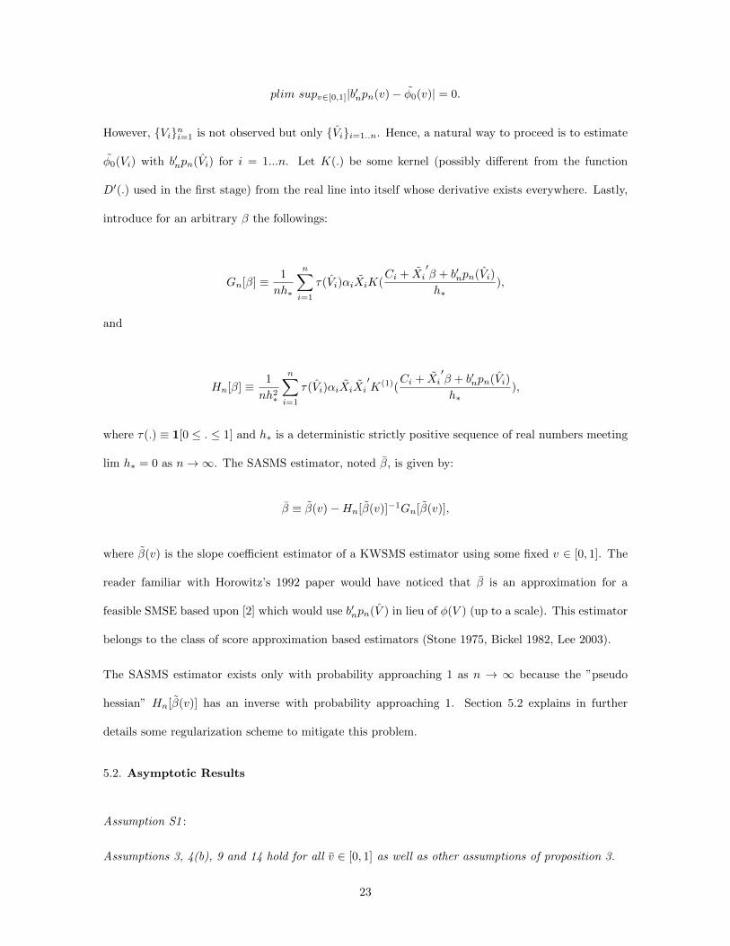
plim supv∈[0,1]|b′npn(v)− φ0(v)| = 0.

However, Vini=1 is not observed but only Vii=1..n. Hence, a natural way to proceed is to estimate

φ0(Vi) with b′npn(Vi) for i = 1...n. Let K(.) be some kernel (possibly different from the function

D′(.) used in the first stage) from the real line into itself whose derivative exists everywhere. Lastly,

introduce for an arbitrary β the followings:

Gn[β] ≡ 1

nh∗

n∑i=1

τ(Vi)αiXiK(Ci + Xi

′β + b′npn(Vi)

h∗),

and

Hn[β] ≡ 1

nh2∗

n∑i=1

τ(Vi)αiXiXi′K(1)(

Ci + Xi′β + b′npn(Vi)

h∗),

where τ(.) ≡ 1[0 ≤ . ≤ 1] and h∗ is a deterministic strictly positive sequence of real numbers meeting

lim h∗ = 0 as n→∞. The SASMS estimator, noted β, is given by:

β ≡ β(v)−Hn[β(v)]−1Gn[β(v)],

where β(v) is the slope coefficient estimator of a KWSMS estimator using some fixed v ∈ [0, 1]. The

reader familiar with Horowitz’s 1992 paper would have noticed that β is an approximation for a

feasible SMSE based upon [2] which would use b′npn(V ) in lieu of φ(V ) (up to a scale). This estimator

belongs to the class of score approximation based estimators (Stone 1975, Bickel 1982, Lee 2003).

The SASMS estimator exists only with probability approaching 1 as n → ∞ because the ”pseudo

hessian” Hn[β(v)] has an inverse with probability approaching 1. Section 5.2 explains in further

details some regularization scheme to mitigate this problem.

5.2. Asymptotic Results

Assumption S1 :

Assumptions 3, 4(b), 9 and 14 hold for all v ∈ [0, 1] as well as other assumptions of proposition 3.

23

Comments: This ensures that the conclusion of proposition 2 and 3 holds using any fixed value of v

chosen in [0, 1]. The choice of [0, 1] is purely symbolic and can be replaced by any compact set of R

for which the above assumptions hold by means of an appropriate normalization.

Assumption S2 :

There exists a sample size N such that for each v in [0, 1] the sequence E|θ(v) − θ(v)|2n≥N is

monotone.

Comments: This is a dominance condition which ensures a uniform rate of convergence (in the outer

probability sense) for the KWSMS estimator θ(v) over [0, 1]. Under assumption S1 it is known that

for each v, the sequence of mean squared errors converges to 0. This however requires no oscillations

if the sample size is large enough.

Assumption S3 :

(a) φ(.) is p times continuously differentiable on [0, 1] for some p ≥ 1. (b) There exists some finite

constant C and some γ ∈ (0, 1] such that |φ(p)(v1)−φ(p)(v2)| ≤ C|v1−v2|γ for all (v1, v2) ∈ [0, 1]×[0, 1].

Comments: Condition (a) is explicit with the additional slightly stronger requirement in (b) that

the pth derivative of Med(ε|V = v) be Holder continuous. Then the nuisance function φ(.) can be

approximated (up to scale) arbitrary well by many linear Sieves methods.

Assumption S4 :

ρ(n) is a given sequence of natural numbers such that ρ(n)/n < 1 for all n and ρ(n)→∞ as n→∞.

Comments: Let ||f ||sup for a real valued function f : [0, 1] → R denotes the sup norm on [0, 1].

Under assumption S3 and assumption S4 there exists a known basis of functions fjj≥1 such that

its linear span Eρ = f : [0, 1] → R, f =∑ρj=1 ajfj , aj ∈ R can approximate the control function

φ(.) arbitrary well in the sense that infEρ(n)||f − φ||sup → 0 as n → ∞ (see Chen 2007). That is,

defining pn(.)′ = (f1(.), ..., fρ(n)(.)) there exists B′n = (b0,1, ..., b0,ρ(n)) such that B′npn provides a good

approximation of the unknown control function on [0, 1] for n large enough.

24

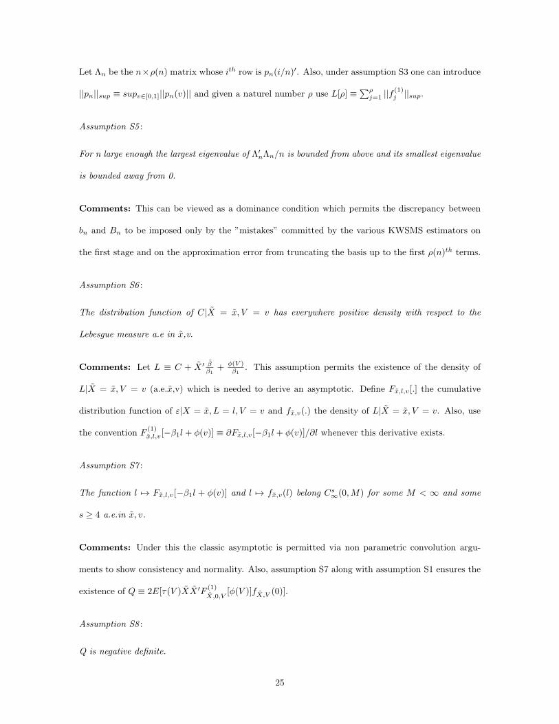
Let Λn be the n×ρ(n) matrix whose ith row is pn(i/n)′. Also, under assumption S3 one can introduce

||pn||sup ≡ supv∈[0,1]||pn(v)|| and given a naturel number ρ use L[ρ] ≡∑ρj=1 ||f

(1)j ||sup.

Assumption S5 :

For n large enough the largest eigenvalue of Λ′nΛn/n is bounded from above and its smallest eigenvalue

is bounded away from 0.

Comments: This can be viewed as a dominance condition which permits the discrepancy between

bn and Bn to be imposed only by the ”mistakes” committed by the various KWSMS estimators on

the first stage and on the approximation error from truncating the basis up to the first ρ(n)th terms.

Assumption S6 :

The distribution function of C|X = x, V = v has everywhere positive density with respect to the

Lebesgue measure a.e in x,v.

Comments: Let L ≡ C + X ′ ββ1+ φ(V )

β1. This assumption permits the existence of the density of

L|X = x, V = v (a.e.x,v) which is needed to derive an asymptotic. Define Fx,l,v[.] the cumulative

distribution function of ε|X = x, L = l, V = v and fx,v(.) the density of L|X = x, V = v. Also, use

the convention F(1)x,l,v[−β1l + φ(v)] ≡ ∂Fx,l,v[−β1l + φ(v)]/∂l whenever this derivative exists.

Assumption S7 :

The function l 7→ Fx,l,v[−β1l + φ(v)] and l 7→ fx,v(l) belong Cs∞(0,M) for some M < ∞ and some

s ≥ 4 a.e.in x, v.

Comments: Under this the classic asymptotic is permitted via non parametric convolution argu-

ments to show consistency and normality. Also, assumption S7 along with assumption S1 ensures the

existence of Q ≡ 2E[τ(V )XX ′F(1)

X,0,V[φ(V )]fX,V (0)].

Assumption S8 :

Q is negative definite.

25

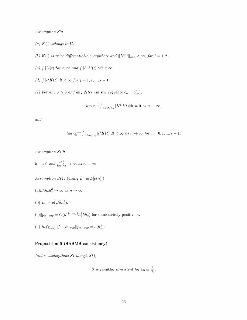
Assumption S9 :

(a) K(.) belongs to Ks.

(b) K(.) is twice differentiable everywhere and ||K(j)||sup <∞, for j = 1, 2.

(c)∫|K(t)|4dt <∞ and

∫|K(1)(t)|2dt <∞.

(d)∫|tjK(t)|dt <∞ for j = 1, 2, ..., s− 1.

(e) For any σ > 0 and any deterministic sequence cn = o(1),

lim c−1n

∫|t|>σ/cn |K

(1)(t)|dt = 0 as n→∞,

and

lim cj−sn

∫|t|>σ/cn |t

jK(t)|dt <∞ as n→∞ for j = 0, 1, ..., s− 1.

Assumption S10 :

h∗ → 0 andnh8∗

log(n) →∞ as n→∞.

Assumption S11 : (Using Ln ≡ L[ρ(n)])

(a)nhhqh6∗ →∞ as n→∞.

(b) Ln = o(√nh3∗).

(c)||pn||sup = O(n(1−γ)/2h3∗hhq) for some strictly positive γ.

(d) infEρ(n)||f − φ||sup||pn||sup = o(h3

∗).

Proposition 5 (SASMS consistency)

Under assumptions S1 though S11,

β is (weakly) consistent for β0 ≡ ββ1.

26

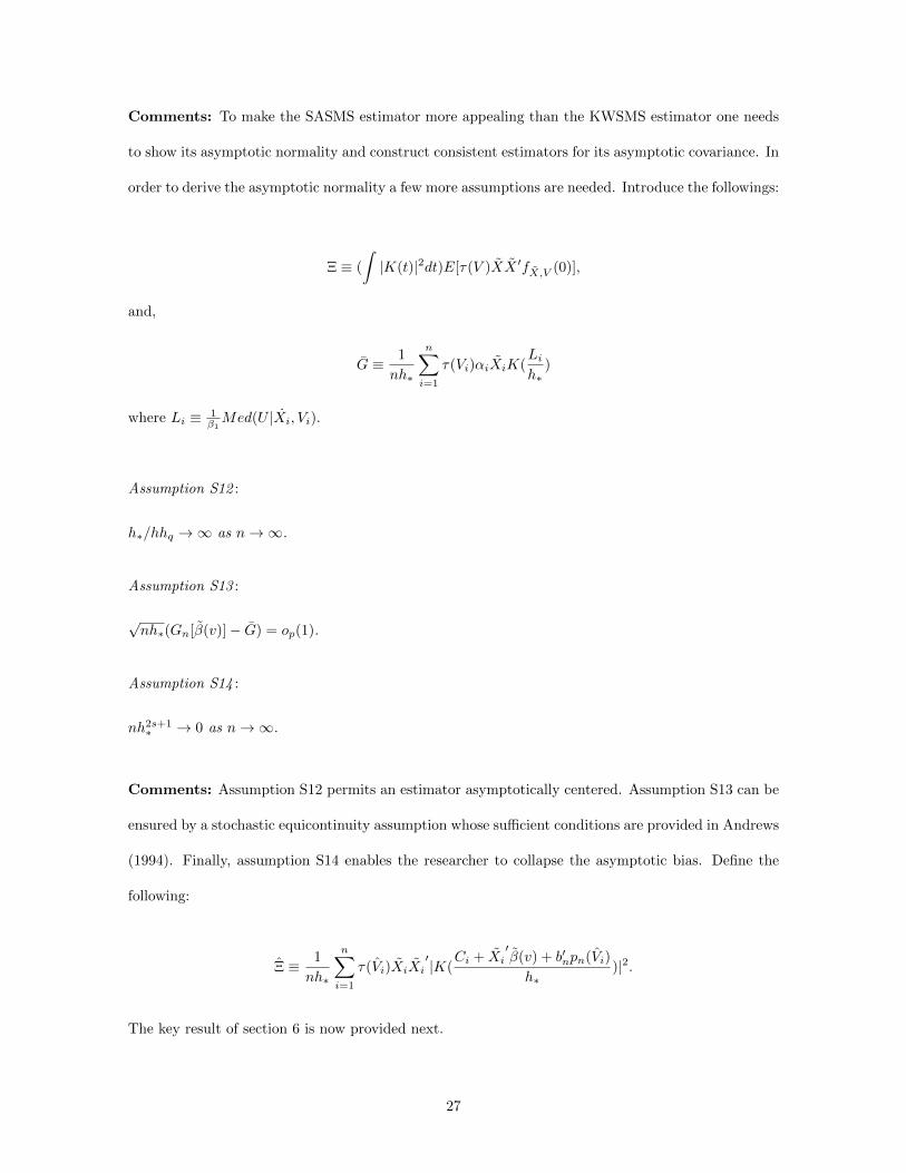
Comments: To make the SASMS estimator more appealing than the KWSMS estimator one needs

to show its asymptotic normality and construct consistent estimators for its asymptotic covariance. In

order to derive the asymptotic normality a few more assumptions are needed. Introduce the followings:

Ξ ≡ (

∫|K(t)|2dt)E[τ(V )XX ′fX,V (0)],

and,

G ≡ 1

nh∗

n∑i=1

τ(Vi)αiXiK(Lih∗

)

where Li ≡ 1β1Med(U |Xi, Vi).

Assumption S12 :

h∗/hhq →∞ as n→∞.

Assumption S13 :

√nh∗(Gn[β(v)]− G) = op(1).

Assumption S14 :

nh2s+1∗ → 0 as n→∞.

Comments: Assumption S12 permits an estimator asymptotically centered. Assumption S13 can be

ensured by a stochastic equicontinuity assumption whose sufficient conditions are provided in Andrews

(1994). Finally, assumption S14 enables the researcher to collapse the asymptotic bias. Define the

following:

Ξ ≡ 1

nh∗

n∑i=1

τ(Vi)XiXi′|K(

Ci + Xi′β(v) + b′npn(Vi)

h∗)|2.

The key result of section 6 is now provided next.

27

Proposition 6

Under assumptions S1 though S14,

√nh∗(β − β0) →d N (0, Q−1ΞQ−1).

Furthermore,

Hn[β(v)] −→p Q and Ξ −→p Ξ.

Comments: Proposition 6 implies that the SASMS estimator achieves a faster rate of convergence

in probability than the KWSMS estimator while still allowing for hypothesis testing. To be more

specific, the SASMS estimator’s rate of convergence is (hhqh∗

)1/2 times that achieved on the KWSMS

estimator which is faster since limhhqh∗

= 0 as n→∞ by assumption S12. It turns out that this is not

the most efficient estimator (in the asymptotic sense) under the assumptions of proposition 6. It is

not very difficult to show that a more efficient CAN estimator is given by:

βE ≡ β(v) + Ξ−1Gn[β(v)],

which yields,

√nh∗(βE − β0) →d N (0,Ξ−1).

This will be subsequently referred to as the ”efficient” SASMS estimator.8

It is important to bear in mind that the SASMS estimator (respectively the ”efficient” SASMS esti-

mator) exists only with probability approaching one as n → ∞ since the matrix Hn[β(v)] defined in

section 5.1 (respectively Ξ as defined on page 27) has an inverse only with probability approaching

one. In finite sample these estimators may thus exhibit a large variance because of the instability

8Indeed, this efficient SASMS estimator requires milder assumptions than those imposed in propositions 5-6. Clearly,

assumption S8 is not needed but also assumptions S9(b), S9(c),S9(e) can be shown to be stronger than required for

deriving consistency and asymptotic normality.

28

of the matrix in question which may be near singular with a strictly positive probability. When the

kernel of assumption S9 has the form K(t) = p(t)1[|t| ≤ 1] for some finite degree polynomial p (see

Muller 1984), one way to mitigate this variability for the SASMS estimator is to compute Hn[β(v)]

replacing K(1)(t) with K(1)c (t) = p(1)(t)1[|t| ≤ 1 + cn] where cn is a deterministic sequence of positive

real numbers satisfying cnh∗→ 0 as n→∞.9

The selection of the bandwidths is not covered in proposition 6 owing to the fact that only a generic

case for any basis fjj≥1 is treated. However, in application one needs to select an appropriate basis

for smooth functions and pick three bandwidths sequences h, hq and h∗ meeting the assumptions of

proposition 6. The next proposition establishes for the power series basis and trigonometric cosine

basis how the bandwidths and sieves’s sequence ρ(n) may be selected up to a scale. The symbol [κ]

for a real number κ will refer to the least lower integer of κ.

Corollary (Bandwidths Admissibility For Power series and Trigonometric cosinus )

Suppose that assumption S1 holds with r > m/3 , assumption S7 holds for some s ≥ 5 and assumption

S3 holds for some p > 4. Also, suppose that others assumptions of proposition 6 hold but assumptions

S4,S10,S11,S12,S14. When pn(v)′ = (f1(v), ..., fρ(n)(v)) is chosen from Power series or Trigonometric

cosinus then the assumptions of proposition 6 are satisfied under the followings:

(a)h ∝ n−a and hq ∝ n−λa, for some a ∈ ( 11+λ+2λm ,

110(1+λ) ) and some λ ∈ ( 3

2m−3 ,min9

2m−9 , 1/3).

(b) h∗ ∝ n−a∗, for some a* ∈ (maxa′, 12s+1,min

1−4a′

6 , p′

6p′+12) where a′ = a(1+λ) and p′ = p−1.

(c) ρ(n) = C0[nν ], for some ν ∈ ( 3a∗p−1 ,

1−6a∗4 ) and some C0 ∈ (0, n

[nν ] ).

Comments: This corollary is based upon the fact that with power series or trigonometric series on

has ||pn||sup = O(ρ(n)) and Ln = O(ρ(n)2) while infEρ(n)||f − φ||sup = O(1/ρ(n)p) (see Chen 2007).

Some lengthy algebra can show that (a),(b) and (c) are sufficient for the conditions of proposition 6 to

9This ”regularized” version for the SASMS estimator has the same limiting distribution because K(1) and K(1)c differ

only when 1 ≤ |t| ≤ 1 + cn under assumption 9, see Lemma 13-14 and proof of proposition 5.

29

hold. However, those are not necessary and assumptions S4,S10,S11,S12,S14 may hold under different

set of conditions which can be found by the researcher on a case to case basis.

6 Monte Carlo Simulations

This section examines the finite sample properties of the estimators put forth in this paper using

Monte Carlo experiments. These estimators are used to estimate the parameter β = 1 when the data

generating process obeys:

Y = 1 if Z + βA+ ε ≥ 0 and Y = 0 otherwise,

A = ΠW + V ,

ε = φ(V ) + e,

where (Z,W ) is a standard bivariate Normal couple of correlation coefficient % , V ∼ N (0, 1), and Π

is set equal to 1. In this experiment three designs are considered satisfying the followings:

Design ST: % = 0.5; φ(V ) = exp(−V 2); e = (1 + Z2 + Z4)T where T is Student with 3 degrees of

freedom.

Design PR: % = 0.5; φ(V ) = 0.5V ; e ∼ N (0, 1).

Design LG: % = 0; φ(V ) = cos(πV ); e ∼ Logistic.

In addition, two other estimators addressing endogeneity for the binary choice model are used. The

first one is the limited information ML estimator10 (LIML) proposed in Rivers and Vuong (1988)

and the second is the artificial two stage least square estimator11 (2SLS) suggested in Lewbel (2000).

10Under the assumptions of Rivers and Vuong (1988) the coefficients are identified up to a different scaling factor. In

our context, the LIML refers thus to the ratio between the LIML estimator of A slope coefficient and Z slope coefficient

since this is how a researcher would estimate our coefficient of interest.11One choice left to the researcher for computing this estimator is the Kernel which is needed for estimating the

density of Z given W, see Lewbel (2000). The Monte Carlo experiments are performed with a normal kernel along with

the bandwidths n−1/6.

30

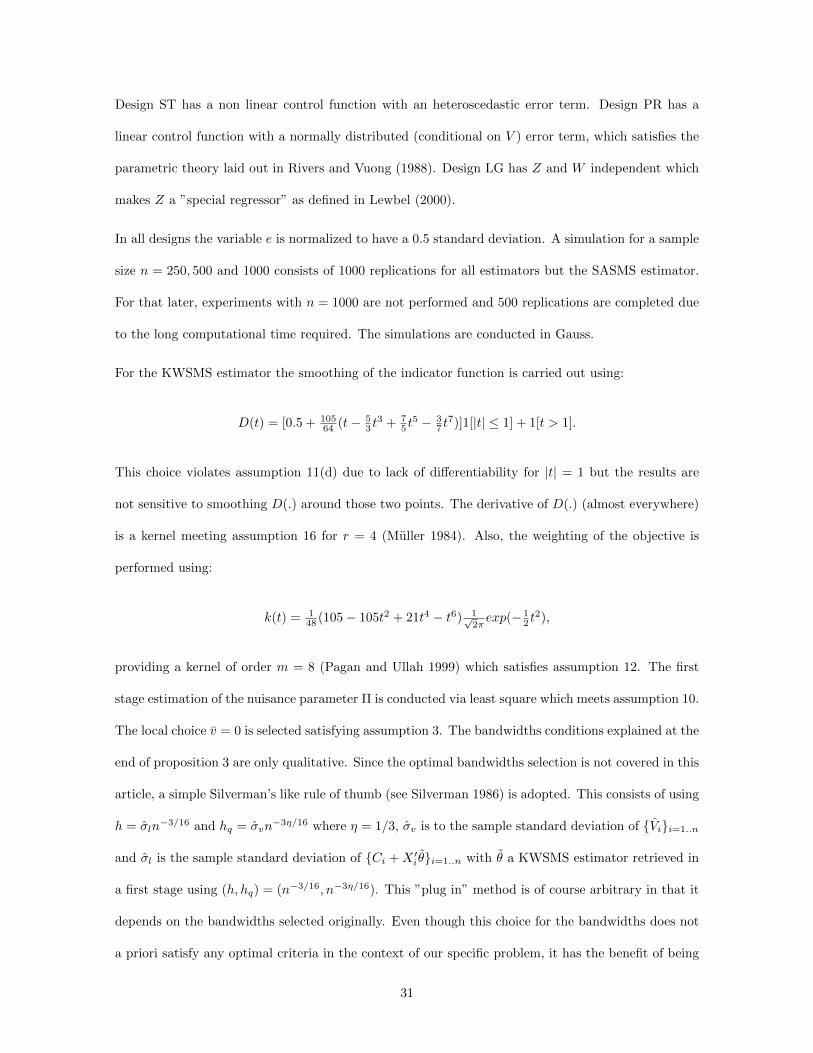
Design ST has a non linear control function with an heteroscedastic error term. Design PR has a

linear control function with a normally distributed (conditional on V ) error term, which satisfies the

parametric theory laid out in Rivers and Vuong (1988). Design LG has Z and W independent which

makes Z a ”special regressor” as defined in Lewbel (2000).

In all designs the variable e is normalized to have a 0.5 standard deviation. A simulation for a sample

size n = 250, 500 and 1000 consists of 1000 replications for all estimators but the SASMS estimator.

For that later, experiments with n = 1000 are not performed and 500 replications are completed due

to the long computational time required. The simulations are conducted in Gauss.

For the KWSMS estimator the smoothing of the indicator function is carried out using:

D(t) = [0.5 + 10564 (t− 5

3 t3 + 7

5 t5 − 3

7 t7)]1[|t| ≤ 1] + 1[t > 1].

This choice violates assumption 11(d) due to lack of differentiability for |t| = 1 but the results are

not sensitive to smoothing D(.) around those two points. The derivative of D(.) (almost everywhere)

is a kernel meeting assumption 16 for r = 4 (Muller 1984). Also, the weighting of the objective is

performed using:

k(t) = 148 (105− 105t2 + 21t4 − t6) 1√

2πexp(− 1

2 t2),

providing a kernel of order m = 8 (Pagan and Ullah 1999) which satisfies assumption 12. The first

stage estimation of the nuisance parameter Π is conducted via least square which meets assumption 10.

The local choice v = 0 is selected satisfying assumption 3. The bandwidths conditions explained at the

end of proposition 3 are only qualitative. Since the optimal bandwidths selection is not covered in this

article, a simple Silverman’s like rule of thumb (see Silverman 1986) is adopted. This consists of using

h = σln−3/16 and hq = σvn

−3η/16 where η = 1/3, σv is to the sample standard deviation of Vii=1..n

and σl is the sample standard deviation of Ci +X ′i θi=1..n with θ a KWSMS estimator retrieved in

a first stage using (h, hq) = (n−3/16, n−3η/16). This ”plug in” method is of course arbitrary in that it

depends on the bandwidths selected originally. Even though this choice for the bandwidths does not

a priori satisfy any optimal criteria in the context of our specific problem, it has the benefit of being

31

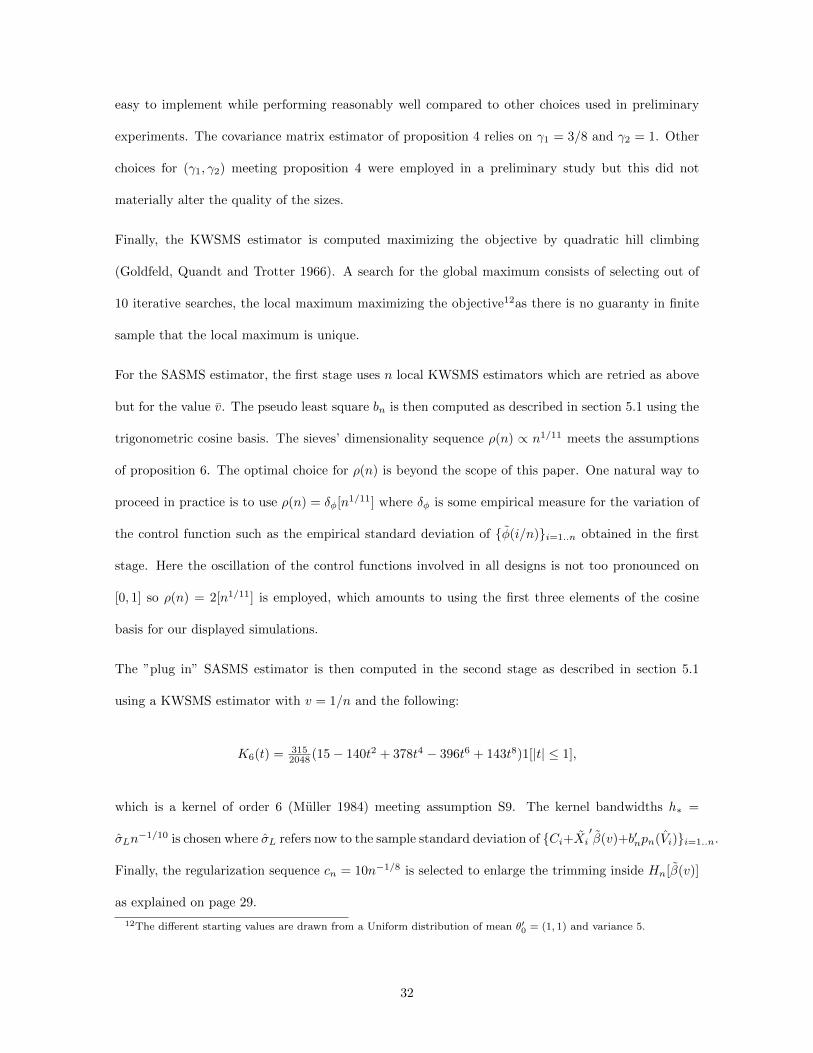
easy to implement while performing reasonably well compared to other choices used in preliminary

experiments. The covariance matrix estimator of proposition 4 relies on γ1 = 3/8 and γ2 = 1. Other

choices for (γ1, γ2) meeting proposition 4 were employed in a preliminary study but this did not

materially alter the quality of the sizes.

Finally, the KWSMS estimator is computed maximizing the objective by quadratic hill climbing

(Goldfeld, Quandt and Trotter 1966). A search for the global maximum consists of selecting out of

10 iterative searches, the local maximum maximizing the objective12as there is no guaranty in finite

sample that the local maximum is unique.

For the SASMS estimator, the first stage uses n local KWSMS estimators which are retried as above

but for the value v. The pseudo least square bn is then computed as described in section 5.1 using the

trigonometric cosine basis. The sieves’ dimensionality sequence ρ(n) ∝ n1/11 meets the assumptions

of proposition 6. The optimal choice for ρ(n) is beyond the scope of this paper. One natural way to

proceed in practice is to use ρ(n) = δφ[n1/11] where δφ is some empirical measure for the variation of

the control function such as the empirical standard deviation of φ(i/n)i=1..n obtained in the first

stage. Here the oscillation of the control functions involved in all designs is not too pronounced on

[0, 1] so ρ(n) = 2[n1/11] is employed, which amounts to using the first three elements of the cosine

basis for our displayed simulations.

The ”plug in” SASMS estimator is then computed in the second stage as described in section 5.1

using a KWSMS estimator with v = 1/n and the following:

K6(t) = 3152048 (15− 140t2 + 378t4 − 396t6 + 143t8)1[|t| ≤ 1],

which is a kernel of order 6 (Muller 1984) meeting assumption S9. The kernel bandwidths h∗ =

σLn−1/10 is chosen where σL refers now to the sample standard deviation of Ci+Xi

′β(v)+b′npn(Vi)i=1..n.

Finally, the regularization sequence cn = 10n−1/8 is selected to enlarge the trimming inside Hn[β(v)]

as explained on page 29.

12The different starting values are drawn from a Uniform distribution of mean θ′0 = (1, 1) and variance 5.

32

Table 1 contains loss measures enabling to assess the quality of the estimators β of β. The Bias

refers to absolute value of the bias i.e.|E(β) − β|. The RM refers to the root mean squared error

i.e.(E|β − β|2)1/2. Table 2 provides the size of the t-test for β relying on the estimators put forth in

this article using the asymptotic critical values for a 1 percent, 5 percent and 10 percent type I error

level.

As displayed on Table 2, the qualitative behaviors of the proposed estimators agree with the asymp-

totic theory developed in this paper. For all designs the bias and RM of the KWSMS estimator

(hereafter noted KWSMSE) consistently shrink as n increases. The same applies to the SASMS es-

timator (hereafter noted SASMSE). For the KWSMSE, on average across bandwidths, a doubling of

the sample size from 500 observations leads close to a 30 percent decrease in the loss measures (i.e.

bias and RM) which is slightly faster than a 24 percent decrease hinted by asymptotic theory.13 The

SASMSE performs poorly when n = 250 relative to the KWSMSE expect for the PR design where a

lower RM is achieved. As suggested by asymptotic theory the performance gap between the SASMSE

and KWSMSE narrows for all designs if n = 500 where the SASMSE outperforms the KWSMSE (in

terms of the RM) except for the LG design. That is, the SASMSE needs a large enough sample to

reach its asymptotic regime. As explained on page 34 the SASMSE defined in section 5.1 may not

even exist in finite sample. The regularization scheme employed for the SASMSE is one out of many

possible means to solve this existence problem at the origin of the larger RM experienced for n = 250.

Motivated by these simulations and those of Table 2 (discussed soon) there seems to be a need to

develop in future research optimal regularization criteria for the SASMSE.

With respect to the overall competitiveness of the proposed estimators, the ST design clearly favors

the KWSMSE (or SASMSE provided n large enough) for every sample size. In that case, the LIML

is inconsistent with a RM twice larger when n = 1000. As expected the PR design unambiguously

supports the LIML, which shows all its efficiency power. In that instance, the KWSMSE (respectively

13proposition 3 suggests that the rate of convergence on the loss is 1/√n1−a−aη which here implies a 24 percent

decrease in losses for a doubling of the sample size. This discrepancy does not undermine our theory because the

moments of√nhhq(θ − θ0) need not to converge unless strong uniform integrability conditions hold, see Chung page

100-101.

33

SASMSE) exhibits a RM approximately 3 times larger for n = 1000 (respectively for n = 500). Finally,

the LG design still favors the LIML (which in not too surprising owing to the fact that the logistic

distribution and normal distribution have relatively close shapes). In that logistic design, the second

most performing estimator when n = 250 is the 2SLS, which is eventually slightly outperformed by

the KWSMS for n ≥ 500.

As exhibited on Table 2, the sizes of the test with the KWSMSE using the asymptotic critical

values are systematically above the asymptotic sizes (even for a sample of 1000 observations). For

instance, the size using the 5 percent critical value ranges from 10 to 29 percent across designs.

Hence, one requires a much larger sample for the asymptotic critical values to provide an accurate

probability coverage for the t-statistic. The same inferential problem affects the smoothed maximum

score estimator (see Horowitz 1992). Even though one can not yet affirm whether the theory of

bootstrapping applies to the KWSMS, the result established in Horowitz (2002) concerning the SMSE

does suggest that the critical value of a bootstrapped t-statistics will provide a more reliable coverage

in finite sample for the KWSMSE. Alternatively, the SASMSE seems to offer somewhat superior

testing capability in terms of sizes, which for n = 500 are closer to the ones promised by asymptotic

theory. This is notably true for the ST design where the type I error is fairly accurately provided by

the asymptotic critical value.

Overall, our Monte Carlo simulations hint that in small sample a KWSMS estimator can be severally

bias when endogeneity is present in the binary choice model. However, if the sample size is sufficiently

large this estimator offers a simple robust estimation technique to obtain accurate estimates as il-

lustrated by the loss measures. However, conducting inferences using the estimated standard errors

relying on proposition 4 may be misleading if the data set is not very large. Also, a second stage

estimation with a SASMS estimator presents clear advantages when the sample size is sufficiently

large especially in terms of testing.

34

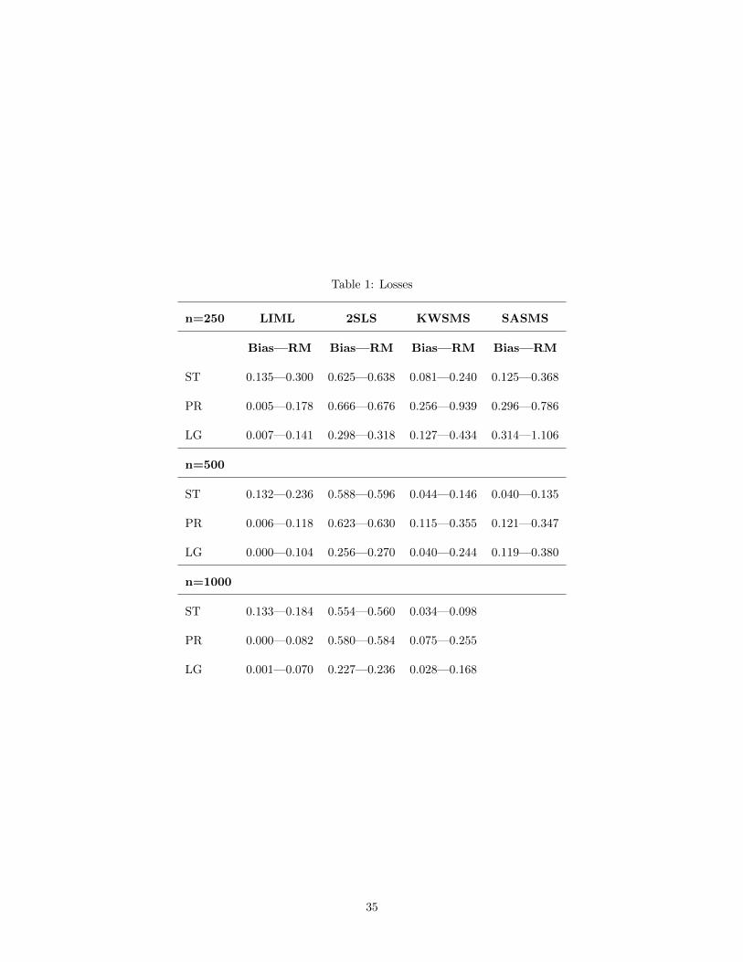
Table 1: Losses

n=250 LIML 2SLS KWSMS SASMS

Bias—RM Bias—RM Bias—RM Bias—RM

ST 0.135—0.300 0.625—0.638 0.081—0.240 0.125—0.368

PR 0.005—0.178 0.666—0.676 0.256—0.939 0.296—0.786

LG 0.007—0.141 0.298—0.318 0.127—0.434 0.314—1.106

n=500

ST 0.132—0.236 0.588—0.596 0.044—0.146 0.040—0.135

PR 0.006—0.118 0.623—0.630 0.115—0.355 0.121—0.347

LG 0.000—0.104 0.256—0.270 0.040—0.244 0.119—0.380

n=1000

ST 0.133—0.184 0.554—0.560 0.034—0.098

PR 0.000—0.082 0.580—0.584 0.075—0.255

LG 0.001—0.070 0.227—0.236 0.028—0.168

35

Table 2: Sizes

n=250 KWSMS SASMS

Nominal level 0.01—0.05—0.10 0.01—0.05—0.10

ST 0.11—0.20—0.27 0.03—0.07—0.09

PR 0.23—0.34—0.42 0.10—0.16—0.21

LG 0.26—0.38—0.45 0.09—0.17—0.20

n=500

ST 0.07—0.12—0.19 0.01—0.02—0.06

PR 0.17—0.26—0.33 0.08—0.14—0.18

LG 0.24—0.36—0.42 0.06—0.10—0.13

n=1000

ST 0.04—0.10—0.16

PR 0.13—0.23—0.30

LG 0.19—0.29—0.35

36

Conclusion

This paper has presented a local version of the control function approach for the binary choice model

to reach consistency when one of the explanatory variables is endogenous. This article has explained

how the objective function of the SMSE can be weighted by means of a kernel taking the control

variables’ estimates as arguments in order to derive an asymptotically centered normal estimator. Fi-

nally, a consistent estimator for the asymptotic covariance matrix has been offered enabling expedient

inferences for applied work whenever a large data set is available. An alternative score approximation

based smoothed maximum score estimator has also been described combining many first stage esti-

mators to obtain a faster rate of convergence. Our Monte Carlo simulations hint that both of these

estimators can provide new tools to estimate the coefficients of interest and conduct hypothesis testing

in the binary choice model when endogeneity is present without having to impose strong distributional

assumptions. We foresee three topics for future research. First, the optimal choice for the bandwidths.

Secondly, the extension of the KWSMS to the case when more than one variable is endogenous and

V is estimated at a non parametric rate. Finally, the testing of endogeneity in a model satisfying (i)

and (ii).

37

References

Abrevaya.J. and Huang.J., 2005. On the bootstrap of the maximum score estimator. Econometrica,

Vol 73, 1175-1204.

Amemiya.T., 1978. The estimation of a simultaneous equation generalized probit model. Economet-

rica, Vol 46, 1193-1205 .

Amemiya.T., 1985. Advanced Econometrics. Cambridge, Harvard University Press.

Andrews.D., 1994. Asymptotic for semi parametric econometrics models via stochastic equicontinu-

ity. Econometrica,Vol 62, No. 1.

Bickel.P., 1982. On adaptive estimation. Annals of Statistics, pp 647.

Blundell.R. and Powell.J., 2004. Endogeneity in semi parametric binary response models. Review of

Economic Studies,71, 665-679.

Chaudhuri.P., 1991 Nonparametric estimates of regression quantiles and their local Bahadur repre-

sentation. Annals of Statistics.

Chen.X., 2007. Large sample sieve estimation of semi-nonparametric models. Handbook of Econo-

metrics,Vol 6B..

Chung K. A course in probability theory. Academic press, third edition..

Goldfeld.S. Quandt.R. and Trotte.H., 1966. Maximization by quadratic hill-climbing. Econometrica,

Vol.34, No.3.

38

Heckman.J., 1978. Dummy endogenous variables in a Simultaneous equation system. Econometrica

Vol 46, 931-959.

Hong.H. and Tamer.E., 2003. Endogeneous binary choice model with median restriction. Economics

Letters, Vol 80, 219-225.

Horowitz.J., 1992. A smoothed maximum score estimator for the binary response model. Economet-

rica, Vol 60, No.3.

Horowitz.J., 1993. Semiparametric estimation of a work trip mode choice model. Journal of Econo-

metrics, Vol 58, 49-70.

Horowitz.J., 2002. Bootstrap critical values for tests based on the smoothed maximum score estima-

tor. Journal of Econometrics, Vol 111, 141-167.

Kim.J. and Pollard.D., 1990. Cube root asymptotics. The Annals of Statistics, vol 18, No.1.

Lee.L., 1981. Simultaneous equation models with discrete and censored variables., in: C. Manski

and D. Mc Fadden, eds., Structural analysis of discrete data with economic applications, MIT

press, Cambridge, MA.

Lee.S., 2003. Efficient semi parametric estimation of a partially linear quantile regression model.

Econometric Theory, Vol 19, 1−31.

Lee.S., 2007. Endogeneity in quantile regression models: A control function approach. Journal of

Econometrics Vol 141, No.2.

Lewbel.A., 2000. Semiparametric qualitative response model estimation with unknown heteroscedas-

ticity or instrument variables. Journal of Econometrics Vol 97, 145-177.

39

Manski.C., 1975. Maximum score estimation of the stochastic utility model of choice. Journal of

Econometrics, Vol 3, 205-228.

Manski.C., 1985. Semi parametric analysis of discrete response, asymptotic properties of the maxi-

mum score estimator. Journal of Econometrics, Vol 27, 313-334.

Muller.H., 1984. Smooth optimum kernel estimators of regression curves, densities and modes.

Annals of Statistics 12, 766-774.

Newey.W., 1985. Generalized Method of Moments Specification Testing. Journal of Econometrics,

29, 229-256..

Newey.W., 1985. Semiparametric estimation of limited dependent variables models with endogenous

explanatory variables. Annales de l’Insee, No 59/60, Econometrie non lineaire asymptotique.

Newey.W., 1987. Efficient estimation of limited dependant variable models with endogenous explana-

tory variables. Journal of Econometrics, Vol 36, 230-251.

Newey.W, Powell.J. and Vella.F., 1999. Non parametric estimation of triangular simultaneous equa-

tions models. Econometrica, Vol 67, 565-603.

Pagan.A. and Ullah.A., 1999. Non parametric econometrics. Cambridge University Press.

Pagan.A. and Vella.F., 1989. Diagnostic Tests for Models Based on Individual Data: A Survey.

Journal of Applied Econometrics, vol. 4(S), pages S29-59.

Powell.J., 1986. Censored regression quantiles. Journal of Econometrics, Vol 32, 143-155.

Rivers.D. and Vuong.Q., 1988. Limited information estimation and exogeneity tests for simultaneous

probit models. Journal of Econometrics, Vol 39, 347-366.

40

Rothe.C., 2009. Semiparametric estimation of binary response models with endogenous regressors.

Journal of Econometrics, Vol 153, 51-64.

Smith.R. and Blundell.R., 1986. An exogeneity test for a simultaneous equation tobit model with

an application to Labor supply. Econometrica, Vol 54, 679-685.

Stone.C., 1975. Adaptive maximum likelihood estimators of a location parameter. Annals of Statis-

tics, pp. 267-284.

Szu.H. and Hartley.R., 1987. Fast simulated annealing. Physics letters, Vol 122, 3-4.

41

Appendix

Section A-Relaxing the Median Restriction and Heteroscedastic Endogenous Models

A1. Semi Linear Heteroscedasticity

To clarify the conflict between the key median restriction in [1] and heteroscedasticity considers a fairly general example

taken from Lee 2007:

ε = H(V ) + ϑ(Xs, V )R,

where R|Z,W, V∼ R and (Xs, Xg) forms a partition of X∗ with Dim Xg ≥ 2. That is U = X′gβg + X′sβs + ε where

β = (βs, βg). Here H(.) is some unknown function and ϑ(., .) may not be known a priori. For simplicity suppose that

ϑ(Xs, V ) > 0 a.s. and that the cumulative distribution function of R noted FR(.) is strictly increasing. Assuming that

R has a second moment the error term ε is thus heteroscedastic in (X∗, V ) and it is rapid to show:

Med(ε|Z,W, V ) = H(V ) + ϑ(Xs, V )F−1R (1/2) a.s.

When Med(R) = 0 holds then the restriction in [1] is met. Conversely, when Med(R) 6= 0 it is possible to employ our

estimation procedure whenever ϑ(Xs, V ) is semi linear of the form T (V )+X′sϕ for some unknown T (.) and parameter ϕ.

To see this transformed the model into U = X′gβg+X′s(βs+ϕF−1R (1/2))+e where now Med(e|Z,W, V ) = Med(e|V ) =

H(V ) +T (V )F−1R (1/2) a.s.. In this case, βg and the composite slope βs+ϕF−1

R (1/2) can be estimated consistently via

our estimation method. Thus, unless further restrictions on the parameter βs + ϕF−1R (1/2) are imposed, the estimator

presented in this paper offers a viable approach to estimate and answer inferential questions pertaining only to βg . Yet,

our asymptotic results permit some testing on βs. For instance, letting βs,1 and βs,2 being two slope coefficients of Xs

one can test the null βs,1 > βs,2 or βs,1 = βs,2 which may be the only question of interest in some applied work when

βg,1 and βg,2 represent some elasticities.

Finally, when Med(R) 6= 0 it is possible to extend our estimation procedure when ϑ(Xs, V ) is unknown by using the

partial median restriction Med(ε|Z,W, V ) = Med(ε|Xs, V ) a.s. and viewing (Xs, V ) as the new artificial control variable

(see section A2 below). As when ϑ(Xs, V ) is known to be semi linear, only the slope coefficient of Xg can be estimated

consistently and tested for significance.

A2. Unknown Heteroscedasticity

Let suppose that there exists a partition of X = (Xs, Xg) for which:

Med(ε|X, V ) = Med(ε|Xs, V ).

42

That is, the control is only ”partial” because only Xg is purged after controlling for V. For instance, an heteroscedastic

error term ε = σ(Xs)e where e|Z,W, V ∼ e|V may generate such a partial restriction. As will be explained shortly,

one can without much difficultly extend the framework laid out in section 3-4-5 to identify and consistently estimate

the slope coefficients of the variables purged from the control i.e.Xg . In this section we only treat the extension for the

KWSMS estimator since the adaptation for the SASMS estimator follows straightforwardly from that of the former.

Similarly to section 2, only a local control is needed for the median restriction. Let suppose that ε|xs, v has an absolutely

continuous distribution function and that φ(xs, v) = Med(ε|xs, v) is well defined. The extension in this context requires

the following restriction:

Med(ε|Xg , xs, v) = Med(ε|xs, v) a.s.,

Suppose that p = dimXg is greater than 2. Furthermore, assume that there exists a partition of Xg = (Xg1 , X

g) with

Xg1 |Xg having an absolutely continuous distribution (a.s.) and such that βg1 , the slope coefficient of Xg

1 is non null

(which we take to be positive without loss of generality). Finally, suppose the distribution of V,Xs|Xg is absolutely

continuous (a.s.) with respect to the relevant product measure. Under some regularity conditions similar to those of

proposition 1 one can show:

θ0 = (β0, c0) = Argmaxβ,cE[d(`+ Xg(β − β0) + c− c0)fXg,`

(xs, v)Mxs,v(`)],

where

` = Xg1 + Xgβ0 + c0,

β0 = βg

βg1

, c0 =xs′βs+φ(xs,v)

βg1

,

fXg,`

(xs, v) is the density of Xs, V |Xg , ` evaluated at (xs, v),

and

Mxs,v(`) = 1− 2Fxs,v [−βg1 `+ φ(xs, v)] with Fxs,v [.] the cumulative distribution function of ε|Xs = xs, V = v.

Hence, under a random sampling from (Y,Xs, Xg), assuming the analogue of assumption 9 for v, xs 7→ 1−2F`,xg,xs,v,

[−βg1 `+

φ(xs, v)]fxg,`

(xs, v) a.e.in xg , ` (F`,xg,xs,v,

[.] indicating the cumulative distribution function of ε|`, Xg , Xs, V ) and given

some root n consistent residuals for the control variable one can establish the weak consistency of:

Argmaxβ,c1

nhK−p+1q

∑ni=1 αiD(

Xg1,i

+Xgi

′β+c

h)k( Vi−v

hq,Xsi−xshq

),

where k(t1, t2) is now a multivariate kernel. Additionally, one can without major obstacles show the asymptotic

normality of such an estimator adapting the assumptions of proposition 3 to the multivariate case for k(., .). De-

fine fxg

(`) the density of `|xg , the main changes would involve the analogue of assumptions 14 for ` 7→ Txg

(`) =

43

Mxs,v(`)fxg,`

(xs, v)fxg

(`) a.e.in xg and assuming that E[XX′T(1)

xg(0)] is positive definite. We leave to the reader the

details of this generalization.

Section B-Proof

This section provides the proofs of the propositions. Some notations will be used. ||X|| denotes the Euclidean norm of

a vector X ∈ Rp where p ∈ N and |||M ||| =√traceMM ′ for a real valued Matrix M. For r > 0 and z ∈ Rp where p ∈ N

define B(z, r) = x ∈ Rp : ||x− z|| < r. The least upper integer of a real number t is noted int[t].

For a given multivariate real value function twice differentiable say F (θ) the symbol ∇F (θ) denotes its gradient and

HF (θ) its hessian evaluated at θ. Also the sequences of real value functions Dn(t) = D(t/h) , Kn(t) = 1hK(t/h) and

kn(t) = 1hqk(t/hq) are used. However, the notations kn(V ) = 1

hqK(V−v

hq) and kn(V ) = 1

hqK( V−v

hq) are employed

which should be kept in mind.

Moreover, the objectives,

Sn(θ) = 1nhq

∑ni=1 αiD(

Ci+X′iθ

h)k( Vi−v

hq),

and

Sn(θ) = 1nhq

∑ni=1 αiD(

Ci+X′iθ

h)k(Vi−v

hq) are used.

For an arbitrary real number v use:

Sn(θ, v) = 1nhq

∑ni=1 αiD(

Ci+X′iθ

h)k( Vi−v

hq)

and

Sn(θ, v) = 1nhq

∑ni=1 αiD(

Ci+X′iθ

h)k(Vi−v

hq).

The gradient of Sn(θ, v) with respect to θ is noted ∇Sn(θ, v) and its Hessian HSn(θ, v). Similarly, ∇Sn(θ, v) and

HSn(θ, v) are used. Write θ0(v)′ = 1β1

(φ(v), β) whenever φ(v) exists. The notation λMin[A]and λMax[A] for a

symmetric matrix A will refer to the smallest (respectively largest) eigenvalue of A. Define P ? the outer probability

measure i.e. P ?(E) = inf∑P (Ei)|E ⊆ ∪Ei, Ei ⊆ =. Given a sequence of random variables Xn (not necessarily =-

measurable) define plim?Xn = 0 if for any δ > 0 there exists a natural number N such n ≥ N implies P ?[|Xn| > δ] < δ.

When unspecified the term lim is to be understood with respect to n→∞. Finally, the complement of a set E will be

noted E′.

Lemma 1: Under assumptions 2-4,6,9,11-13 and 15

(i) plim ||Sn − ESn||supΘ = 0. (ii) lim ||ESn − S||supΘ=0.

proof (i): Let gn(θ) = Sn(θ)− ESn(θ). We have:

44

gn(θ) = 1n

∑ni=1 αiDn(`i +X′∆)kn(Vi)− E[αiDn(`i +X′∆)kn(Vi)]

Notice that |αiDn(`i + X′∆)kn(Vi) − E[αiDn(`i + X′∆)kn(Vi)]| ≤ ||Dn||sup||k||sup 1hq

where ||Dn||sup||k||sup is a

constant by assumption 11 and 12. Also using a change of variable provides :

EX,`|kn(Vi)|2 = 1hq

∫|k(t)|2fX,`(v + thq)dt = O( 1

hq)a.s.

due to assumption 12 and 9. Using this last finding and the fact the D(.) is a bounded function provides:

Var [αiDn(`i +X′∆)kn(Vi)] ≤ E|Dn(`i +X′∆)|2|kn(Vi)|2 = O( 1hq

).

It follows by the Bennett’s inequality (1962) that given δ > 0 arbitrary there exists a strictly positive constant C(δ)

such that:

P [|gn(θ)| > δ] ≤ 2e−nhqC(δ)

(1)

and lim |gn(θ)| = 0 a.s. follows by the Borel-Cantelli lemma because of assumption 13. Finally, to show that the

convergence is uniform consider the standard argument using non overlapping coverings (Horowitz 1992 lemma 7 or

Spady and Klein 1993 lemma 1) of our compact set (assumption 8) with subsets of RK such that the distance between

two points in each subset is strictly less than a positive sequence rn. Let Ck,n for k = 1, ...,Γn denotes such collection

of subsets where the number of coverings Γn will depend on the length of the radius rn. Let θk,nk=1...Γn be some

selected finite grid of points with θk,n ∈ Ck,n. Noticing first that:

||∇gn(θ)||supΘ ≤ c1 1hhq

( 1n

∑||Xi||+ c2)

(where c1 and c2 are constants by assumption 12 and 13 by E[||X||] existence i.e.assumption 15) and that any θ in

some Ck,n implies ||θ − θk,n|| < rn yields:

||gn(θ)||supΘ ≤ rnc1 1hhq

( 1n

∑||Xi||+ c2) + supk=1..Γn |gn(θk,n)|

It then suffices to set the decreasing radius such that rn ∝ log(n)nhhq

yielding:

lim rnc11hhq

( 1n

∑||Xi||+ c2) = 0 a.s.,

45

because lim 1n

∑||Xi|| = E[||X||]a.s. by Kolmogorov’s strong law of large numbers due to our iid assumption and

rn1hhq

= o(1) by assumption 13. Finally, plim supk=1..Γn |gn(θk,n)|=0 follows since for γ > 0 arbitrary and using (1)

one can bound P [supk=1..Γn |gn(θk,n)| > γ] owing to:

P [⋃k=1..Γn

|gn(θk,n)| > γ] ≤∑Γnk=1 P [|gn(θk,n)| > γ] ≤ 2Γne−nhqC(γ)

where lim Γne−nhqC(γ) = 0 because Γn ∝ int[(1/rn)K ]. Hence, plim||gn(θ)||supΘ = 0 is established.

proof(ii): step1: Our iid assumption and iterated expectation provide:

ESn(θ) = E[Dn(`+X′∆)kn(V )EX,`,V (α)]

where

EX,`,V (α) = 1− 2FX,`,V (−β1`+ φ(v))

FX,`,V (.) indicating the distribution function of ε|X, `, V . Iterating again gives:

ESn(θ) = E[Dn(`+X′∆)EX,`kn(V )EX,`,V (α)]

where,

EX,`kn(V )EX,`,V (α)] =∫gX,`(v)kn(v)dv, and

gX,`(v) = [1− 2FX,`,v(−β1`+ φ(v)][fX,`(v)].

Using a change of variable with t = v−vhq

and assumptions 2 and 4 further provides:

EX,`kn(V )EX,`,V (α) =∫gX,`(v + thq)k(t)dt a.s

Also by assumption 9(a), there exists σ > 0 and a natural number m ≥ 2 such that on In = |t| < σ/hq:

gx,`(v + thq) = gx,`(v) +∑m−1j=1

1j!g

(j)x,`(v)(thq)j + 1

m!g

(m)x,` (ξ(x, `))(thq)m a.e.in x, `,

for some ξ(x, `) meeting |ξ(x, `)− v| < σ where for |v − v| < σ,

g(j)x,`(v) =

∑jk=0

1k!(j−k)!

j[fx,`(v)](j−k)

with

[1− 2Fx,`,v(−β1`+ φ(v)](j) = ∂j

∂jv1− 2Fx,`,v(−β1`+ φ(v)) and [fx,`(v)](j) = ∂j

∂jvfx,`(v) for j = 1...m.

46

Simplifying and using assumption 12 offers:

∫gx,`(v + thq)k(t)dt =

gx,`(v)− gx,`(v)∫I′nk(t)dt−

∑m−1j=1

g(j)x,`

(v)

j!hjq

∫I′ntjk(t)dt+

hmqm!

∫Ing

(m)x,` (ξ(x, `))tmk(t)dt+

∫I′ngx,`(v + thq)k(t)dt

a.e.in x, `.

Furthermore, |gx,`(v)| < M∗1 for all v, |g(j)x,`(v)| < M∗1 for j = 1, ...,m− 1 and |g(m)

x,` (ξ(x, `))| < M∗1 a.e in x, ` for some

finite constant M∗1 by assumption 9(a). It follows that:

h−mq |∫gx,`(v + thq)k(t)dt− gx,`(v)| ≤M∗1in a.e in x, `,

(1’)

where in = 2h−m∫I′n|k(t)|dt +

∑m−1j=1

hj−mq

j!

∫I′n|tjk(t)|dt + 1

m!

∫|tmk(t)|dt is a bounded sequence by assumption

12(d).

Consequently,

EX,`kn(V )EX,`,V (α)] = gX,`(v) +Rn a.s

where gX,`(v) is given as in proposition 1 due to EX,`,V=v(α) = 1−2FX,`,v [−β1`+φ(v)] and |Rn| = O(hmq ) a.s. by our

finding in (1’)and assumptions 12(d). Furthermore, |gX,`(v)| is bounded almost surely by some real number Mv < ∞

(under assumption 4) yielding:

|ESn(θ)− S(θ)| ≤MvE[|Dn(`+X′∆)− d(`+X′∆)|] +O(hmq ).

Step 2: Subsequently, it is straightforward to establish lim Dn = d a.e. by assumption 11 (where the convergence may

not hold at the origin). It follows (by Horowitz 1992, lemma 4) that given ε > 0 arbitrary there exists some Borel set

B of Lebesgue measure strictly less than ε where lim ||Dn − d||supB′ = 0 holds. Consequently:

|ESn(θ)− S(θ)| ≤Mv(||D||sup + 1)P [`+X′∆ ∈ B] +Mv ||Dn − d||supB′ +O(hmq ).

step 3: Finally, the cumulative distribution function of `|X = x is absolutely continuous with respect to the Lebesgue

measure a.e.in x by assumption 4(a) with furthermore a density whose essential supremum is bounded by some constant

M a.e.in x by assumption 9(b)implying:

P [`+X′∆ ∈ B] < Mε uniformly over Θ,

47

where we used P [`+X′∆ ∈ B] = EPX [` ∈ B−X′∆] and the invariance of the Lebesgue measure to translation. Hence:

|ESn(θ)− S(θ)| ≤Mv(||D||sup + 1)Mε+Mv ||Dn − d||supB′ +O(hmq ),

withO(hmq ) = o(1) by assumption 13. It follows that for any δ > 0 one can pick B to have measure ε < δ3M(||D||sup+1)Mv

so there exists a sample size N(δ) such that n ≥ N(δ) implies |ESn(θ) − S(θ)| < δ uniformly over Θ concluding (ii).

QED

Lemma 2: Let G be some function in C2∞(M) for some finite real number M , K(.) satisfying assumption 16 and hn

some strictly positive sequence converging to 0 as n approaches infinity. Then we have:

lim ||µn(x)−G(1)(x)||sup = 0 where µn(x) = 1h

∫−K(1)(t)G(x+ th)dt

proof: Define En = t ∈ R : |t| ≤ 1h and use the indicator function 1E(t) = 1 if t belongs to a real Borel set E. Given

an arbitrary real number x we have:

µn(x) = In1(x) + In2(x)

where

In1(x) = 1h

∫−K(1)(t)G(x+ th)1E′n (t)dt

and

In2(x) = 1h

∫−K(1)(t)G(x+ th)1En (t)dt

The first part is easy as:

|In1(x)| ≤ ||G||sup 1h

∫|K(1)(t)|1E′n (t)dt

This results in lim |In1(x)| = 0 uniformly in x by the tail property of the Kernel K(.) (assumption 16(d)). Furthermore,

integrating by part over En yields:

In2(x) = In3(x) + In4(x)

where

In3(x) = − 1hK(t)G(x+ th)|t∈En and In4(x) =

∫K(t)G(1)(x+ th)1En (t)dt

48

Moreover, |In3(x)| ≤ 2||G||sup 1h|K( 1

h)| because the Kernel is symmetric by assumption. As |t||K(t)| tends to 0 as t

tends to infinity by assumption 16 we obtain lim |In3(x)| = 0 uniformly in x. Consequently we have :

µn(x)−G(1)(x) =∫

[G(1)(x+ th)1En (t)−G(1)(x)]K(t)dt+ en(x)

where the function en(x) = In1(x) + In3(x) meets ||en||sup = o(1) by our previous findings. Simplifying gives:

|µn(x)−G(1)(x)| ≤∫|G(1)(x)||K(t)|1E′ndt+

∫|G(1)(x+ th)−G(1)(x)|K(t)|dt+ |en(x)|

≤ ||G(1)||sup∫|K(t)|1E′ndt+ hL

∫|t||K(t)dt+ ||en||sup

where L is a constant as the derivative of G(.) is Liptchitz due to G belonging to C2∞(M). Finally, using lim∫

|K(t)|1E′ndt=0 (by the Lebesgue’s Dominated Convergence Theorem) and∫|t||K(t)|dt <∞ by assumption 16 finishes

the proof. QED

Lemma 3: Under assumptions 1-4,6,8,9,12-17

plim HSn(θ) = −E[XX′T(1)X (−X′∆)] where ∆ = θ − θ0 uniformly over Θ.

proof: We will first use HS∗n(θ) = 1n

∑ni=1 αiXiX

′i1|XiX′i|≤an

K(1)n (`i+X

′i∆)kn(Vi) (where |.| here is to be understood

component wise) where an ∝ h−2log(n). We will start showing the uniform consistency of HS∗n since it is easier to

establish. Then, we will have left to show plim HSn(θ) − HS∗n(θ) = 0 uniformly over Θ. The notation H(θ) =

−E[XX′T(1)X (−X′∆)] is adopted.

step1: Let ’s show plim HS∗n(θ)− EHS∗n(θ) = 0 uniformly over Θ. We have:

HS∗n(θ)− EHS∗n(θ) =

1n

∑ni=1 αiXiX

′i1|XiX′i|≤an

K(1)n (`i +X′i∆)kn(Vi)− E[αiXiX

′i1|XiX′i|≤an

K(1)n (`i +X′i∆)kn(Vi)].

By assumption 12 and 16 we get :

|αiXiX′i1|XiX′i|≤anK(1)n (`i +X′i∆)kn(Vi)− E[αiXiX

′i1|XiX′i|≤an

K(1)n (`i +X′i∆)kn(Vi)]| = O( an

h2hq)

(2)

Also, by assumption 12 and 9 and a change of variable it is rapid to find EX,`[|kn(V )|2] ≤ C1hq

a.s. for some finite

constant C1 and similarly by Assumption 14 and 16 that EX [|K(1)n (`i +X′i∆)|2] ≤ C2

h3 a.s. for some finite constant C2.

Hence, by iterated expectations first with respect to X, ` and then with respect to X we obtain the inequality:

49

E[|XiX′i|21|XiX′i|≤an|K(1)n (`i +X′i∆)|2|kn(Vi)|2] ≤ C1C2

h3hqE[|XiX′i|2]

and because E[|XiX′i|2] exists by assumption 15:

V ar[αiXiX′i1|XiX′i|≤an

K(1)n (`i +X′i∆)kn(Vi)] = O( 1

h3hq)

(3)

Combining (2) and (3) suffices for applying again the Bennett’s inequality implying that for any δ > 0 arbitrary real

number there exist two strictly positive constants ν1 and ν2 such that:

P [|HS∗n(θ)− EHS∗n(θ)| > δ] ≤ 2e−nh3hqδ2

ν1+ν2anh

and plim |HS∗n(θ)−EHS∗n(θ)| = 0 follows since limnh4hqlog(n)

=∞ by assumption 17. Subsequently, we have the bounding:

∂∂θ|αiXiX′i1|XiX′i|≤anK

(1)n (`i +X′i∆)kn(Vi)| ≤ O( an

h3hq)

due to ||K(2)||sup||k||sup being a finite constant by assumptions 12 and 16. Hence, choosing a non overlapping covering

with balls whose side length rn satisfies rnanh3hq

= o(1) will provide plim |HS∗n(θ) − EHS∗n(θ)| = 0 uniformly over Θ

by a similar argument as that used for lemma 1.

step2: Let ’s now show lim EHS∗n(θ)−H(θ) = 0 uniformly over Θ.

By assumption 6 we obtain:

E[HS∗n(θ)] = E[XX′1|XX′|≤anK(1)n (`+X′∆)EX,`kn(V )EX,`,V (α)]

Invoking assumptions 9 and 12 and employing the same approach as in lemma 1(ii) provides:

EX,`kn(V )EX,`,V (α) = gX,`(v) +Rna.s. with Rn = O(hmq )a.s.

it follows that:

E[HS∗n(θ)] = A1,n(θ) +A2,n(θ)

where

A1,n(θ) = E[XX′1|XX′|≤anK(1)n (`+X′∆)gX,`(v)]

and

A2,n(θ) = E[XX′1|XX′|≤anK(1)n (`+X′∆)Rn]

First, by assumption 15 and 16 we can use the fact that (where fX(.) indicates the density of `|X):

50

EX|K(1)n (`+X′∆)| =

∫1h|K(1)(t)|fX(th−X′∆)dt ≤M2

∫1h|K(1)(t)|dt a.s. for some finite constant M2,

and the existence of E|XX′| (i.e.assumption 15) to derive:

|E[XX′1|XX′|≤anK(1)n (`+X′∆)Rn]| = O(

hmqh

).

This proves lim A2,n(θ) = 0 uniformly over Θ since O(hmqh

) = o(1) by assumption 17.

Secondly, using µn(X,∆) = EXK(1)n (`+X′∆)gX,`(v) and some simplifications furnishes:

A1,n(θ)−H(θ) = E[XX′1|XX′|≤anµn(X,∆) + T(1)X (−X′∆)] + E[XX′1|XX′|>anT

(1)X (−X′∆)]

But notice that EXK(1)n (`+X′∆)gX,`(v = 1

h

∫TX(th−X′∆)K(1)(t)dt where Tx(`) = gx,`(v)fx(`). Under assumption

14 and assumption 16 the conditions of lemma 2 holds (a.e. in x) yielding:

| 1h

∫TX(th−X′∆)K(1)dt+ T

(1)X (−X′∆)| ≤M2

2 bn + 2M22 cn + 4hM2

2 a.s for some finite constant M2,

where bn and cn are deterministic sequences vanishing to 0 as n approaches infinity. This last finding along with E|XX′|

existence establishes that:

lim E[XX′1|XX′|≤anµn(X,∆) + T(1)X (−X′∆)] = 0 uniformly over Θ.

Finally, |T (1)X (−X′∆)| is almost surely bounded by a finite constant (independently of θ) by assumption 14, E|XX′|

exists and the sequence an meets lim an =∞. Thus, the Dominated Convergence Theorem directly yields:

lim E[XX′1|XX′|>anT(1)X (−X′∆)] = 0

Hence, lim A1,n(θ) = H(θ) uniformly over Θ is established and thus lim EHS∗n(θ)−H(θ) = 0 uniformly over Θ.

step 3: Using basic inequalities we find:

||HSn(θ)−HS∗n(θ)||supΘ ≤ 1h2 ||K(1)||sup 1

n

∑ni=1 |XiX′i|1|XiX′i|>an|kn(Vi)|

so that:

51

E[||HSn(θ)−HS∗n(θ)||supΘ] ≤ 1h2 ||K(1)||supE[|XiX′i|1|XiX′i|>an|kn(Vi)|]

where EX,`[|kn(Vi)|] ≤ M1

∫|k(t)|dt a.s. which is rapid to show by change of variable in the integral along with

assumption 9. Consequently:

E[||HSn(θ)−HS∗n(θ)||supΘ] ≤M1(∫|k(t)|dt) 1

h2E[|XiX′i|1|XiX′i|>an]

But E|XiX′i|2 <∞ from assumption 7 so by the Cauchy-Schwartz’s inequality we can assert:

E[|XiX′i|1|XiX′i|>an] ≤ E|XiX′i|21/2P [|XiX′i| > an]1/2

and by the Tchebychev’s inequality:

P [|XiX′i| > an] ≤ E|XiX′i|2

a2n.

Since∫|k(t)|dt <∞ (i.e.assumption 12) and lim anh2 =∞ we have established:

lim E[||HSn(θ)−HS∗n(θ)||supΘ] = 0

and lemma 3 follows by a triangular inequality using step 1 and step 2. QED

Lemma 4:Under assumptions 9,12,14-16

E[∇Sn(θ0)] = O(hmq ) +O(hr).

proof: Under the iid sampling (assumptions 6)we obtain:

E[∇Sn(θ0)] = E[αXKn(`)kn(V )] = E[XKn(`)kn(V )EX,`,V (α)]

where

EX,`,V (α) = 1− 2FX,`,V [−β1`+ φ(v)]

and similarly to lemma 1 using assumption 9 and 12 permits to show :

EX,`kn(V )EX,`,V (α)] = gX,`(v) +Rn a.s

52

where |Rn| = O(hmq ) a.s. which henceforth returns:

E[∇Sn(θ0)] = B1,n +B2,n

where

B1,n = E[XKn(`)gX,`(v)]

and

B2,n = E[XKn(`)Rn]

First notice that |E[XKn(`)Rn]| ≤ O(hmq )E[|X||Kn(`)|] and that E[|X||Kn(`)|] = E[|X|EX|Kn(`)|] is bounded due

to:

EX|Kn(`)| =∫fX(th)|K(t)|dt ≤M2

∫|K(t)|dt a.s.,

for some finite constant M2 (fX(.) indicating the density of `|X) by assumptions 14 and 16. Hence, B2,n = O(hmq ) is

established. Secondly, we can rewrite B1,n by iterating with respect X yielding:

B1,n = E[Xρn(X)]

where ρn(X) = EXKn(`)gX,`(v) =∫TX(`)Kn(`)d` with TX(`) = gX,`(v)fX(`). Since by assumptions 14, Tx(`) , as

a function of `, is r ≥ 2 times continuously differentiable everywhere with bounded jth derivatives for j = 1...r (a.e.in

x) we can use the same approach as in lemma 1 but this time with a change of variable t = `h

”Taylorizing” Tx(th)

around 0 at order r − 1 and invoking assumption 15 to find:

ρn(X) = TX(0) +R′n a.s.,

where TX(0) = 0 a.s. since FX,0,v [φ(v)] = 1/2 a.s. by assumption 3. Also R′n = O(hr)a.s. is straightforward to establish

using the existence of some constant M such that |T (r)x (`)| < M a.e.in x (from assumptions 14) and the same bounding

principle as given in equation(1) of lemma 1. Because E|X| exists by assumption 15 we have also B1,n = O(hr) which

concludes lemma 4. QED

Lemma 5: Under assumptions 9,11,12,14-17

53

√nhhq∇Sn(θ0)→d N (0,Σ)

proof: It will be convenient to note si,n =√hhqαiXiKn(`i)kn(Vi) and ui,n = E[si,n] for i=1...n. The structure of

the proof is as follows. First, we will show that√nhhq(∇Sn(θ0)− E[∇Sn(θ0)])→d N (0,Σ). Then, we will prove lim√

nhhqE[∇Sn(θ0] = 0. We have thus:

√nhhq(∇Sn(θ0)− E[∇Sn(θ0)]) = 1√

n

∑ni=1 si,n − ui,n

step1: We will first show some preliminary results. Let δ > 0 be some arbitrary constant. Notice that under assumptions

9,11,12,16 and using a change of variable in the integral as in lemma 1 we have:

EX,`| 1√hqk(V−v

hq)|2+δ = 1

hδ/2q

∫|k(t)|2+δfX,`(v + thq)dt ≤ M1

hδ/2q

∫|k(t)|2+δdt a.s. for some constant M1

(4)

Similarly but using assumptions 14 15 and 16 returns:

EX | 1√hK( `

h)|2+δ| ≤ M2

hδ/2q

∫|K(t)|2+δdt a.s. for some constant M2

(5)

Letting Ln =∑ni=1 |

si,n−ui,n√n

|2+δ we obtain under assumption 6:

E[Ln] ≤ n−δ/2E|si,n − ui,n|2+δ ≤ 21+δn−δ/2E|si,n|2+δ

where E|si,n|2+δ = E[|X|2+δ| 1√hK( `

h)|2+δ| 1√

hqk(V−v

hq)|2+δ]. Using (4) and (5) along with assumptions 15(a) and

16(b) ensures that there exists some δ > 0 meeting:

E|si,n|2+δ = O( 1

hδ/2q hδ/2

)

and consequently lim E[Ln] = 0 for some some δ > 0 holds because of our choice for the bandwidths meeting lim

nhqh =∞ by assumption 17.

step 2: Additionally,

E[si,ns′i,n] = E[XX′ 1

h|K( `

h)|2Pn(X, `)]

54

where

Pn(X, `) = EX,` 1hq|k(V−v

h)|2 =

∫1hq|k( v−v

hq)|2fX,`(v)dv.

Moreover, a change of variable t = v−vhq

and a similar reasoning used to derive (1′) of lemma 1 invoking assumption

9(a), 12(b) and 16(c)− (d) provides:

Pn(X, `) =∫fX,`(v + thq)|k(t)|2dt = fX,`(v)

∫|k(t)|2dt+Rn, where Rn = O(hq) a.s.

Thus, we obtain:

E[si,ns′i,n] =

∫|k|2E[XX′ 1

h|K( `

h)|2fX,`(v)] + E[XX′ 1

h|K( `

h)|2Rn]

Moreover, it is easy to show from assumption 14 and a change of variable that |E[XX′ 1h|K( `

h)|2]| is bounded by

M2

∫|K|2E|XX′| <∞ from assumptions 15(a)and 16(b). As a result we find :

E[si,ns′i,n] =

∫|k|2E[XX′ 1

h|K( `

h)|2fX,`(v)] + o(1)

Lastly, assumption 9 and assumption 16 yield:

EX [ 1h|K( `

h)|2fX,`(v)] =

∫µX(`) 1

h|K( `

h)|d`

where µx(`) = fx,`(v)fx(`) is continuous and meets |µx(.)| < C for some finite constant C (a.e. in x) by assumptions

14. Thus, changing the variable into t = `h

provides:

EX [ 1h|K( `

h)|2fX,`(v)] =

∫µX(th)|K(t)|2dt

and two consecutive applications of the Dominated Convergence Theorem furnishes:

lim EX [ 1h|K( `

h)|2fX,`(v)] = µX(0)

∫|K(t)|2dt a.s.,

and

lim E[XX′EX 1h|K( `

h)|2fX,`(v)] =

∫|K|2E[XX′µX(0)].

This subsequently offers:

55

lim E[si,ns′i,n] =

∫|k|2

∫|K|2E[XX′µX(0)]

Notice also that lim E[(si,n − ui,n)(si,n − ui,n)′=lim E[si,ns′i,n] due to ui,n =

√hhqE[∇Sn(θ0)] = o(1) by lemma 4

and assumptions 14. Hence, using the conclusion of step 1 and step 2 permits to apply the Lyapunov’s Central Limit

Theorem (Chung p 208) to affirm:

√nhhq(∇Sn(θ0)− E[∇Sn(θ0)])→d N (0,Σ)

Finally,√nhhqE[∇Sn(θ0]) = O(

√nhhqhmq ) + O(

√nhhqhr) by lemma 4 and

√nhhqE[∇Sn(θ0]) = o(1) follows by

assumptions 17. QED

Lemma 6: Under assumptions 6,7 and 10-14

plim||Sn − Sn||supΘ=0

proof: Using the fact that D(.) is bounded by assumption 11 first let us find :

||Sn − Sn||supΘ ≤ ||D||sup 1n

∑ni=1 |kn(Vi)− kn(Vi)|

and ||k(1)||sup is finite by assumption 12(iii) so the mean value theorem further provides:

||Sn − Sn||supΘ ≤ ||D||sup||k(1)||sup 1nh2q

∑ni=1 |Vi − Vi|

finally, using |Vi − Vi| = |W ′i (Π−Π)| and noting C = ||D||sup||k(1)||sup yields:

||Sn − Sn||supΘ ≤ C||Π−Π||h−2q

1n

∑ni=1 ||Wi||

where 1n

∑ni=1 ||Wi|| = Op(1) by assumption 7 and ||Π − Π||h−2

q = Op(h−2q n−1/2) = op(1) by assumption 10 and 13

which shows the claim.

Lemma 7: under assumptions 6,7,10,12,16 and 17

plim ||HSn −HSn||supΘ = 0

proof: Since ||K(1)||sup is finite by assumption 16 we have:

56

||HSn −HSn||supΘ ≤ ||K(1)||sup 1nh2

∑ni=1 |XiX′i||kn(Vi)− kn(Vi)|

where |kn(Vi)−kn(Vi)| ≤ 1h2q||k(1)||sup|W ′i (Π−Π)| by assumption 12. Noting C = ||K(1)||sup||k(1)||sup and simplifying

further yields:

||HSn −HSn||supΘ ≤ C 1nh2h2

q||Π− Π||

∑ni=1 |XiX′i|||Wi||

where 1n

∑ni=1 |XiX′i|||Wi|| = Op(1) by assumption 6-7 and 15 and 1

h2h2q||Π − Π|| = Op( 1

h2h2qn

1/2 ) by assumption 10.

Consequently ||HSn −HSn||supΘ = op(1) by assumption 17. QED

Lemma 8: Under assumptions 6,7,10,11,13,14,16 and 17

plim√nhhq ||∇Sn(θ0)−∇Sn(θ0)|| = 0

proof: Using assumption 11 and |kn(Vi)− kn(Vi)| ≤ 1h2q||k(1)||sup|W ′i (Π−Π)| easily shows that for some constant C:

√nhhq ||∇Sn(θ0)−∇Sn(θ0)|| ≤ C

√nhhq

||Π−Π||h2q

Tn

where Tn = 1nh

∑ni=1 ||Xi|||K( `i

h)|. Now assumptions 13-14-16-17 and a double application of the Dominated Conver-

gence Theorem easily yields lim E[Tn] =∫|K|E[||X||fX(0)] (where fX(0) is the density of `|X evaluated at 0). Also,

under the iid sampling (assumptions 6), V ar(Tn) ≤ 1nh2E[||X||2|K( `

h)|2] and the classic change of variable subsequently

offers:

V ar(Tn) ≤ 1nhE[||X||2

∫|K(t)|2fX(th)dt]

where again the by Dominated Convergence Theorem applied twice establishes that E[||X||2∫|K(t)|2fX(th)dt] is

bounded for:

lim E[||X||2∫|K(t)|2fX(th)dt]=E[||X||2lim

∫|K(t)|2fX(th)dt]=

∫|K(t)|2E[||X||2fX(0)]

Since lim nh =∞ by assumption 17 we conclude that Tn is bounded in probability. Therefore we have:

√nhhq ||∇Sn(θ0)−∇Sn(θ0)|| = Op(

√hhq

h2q

)

57

and the choice of bandwidths from assumption 17 finalizes the proof. QED

Lemma 9: Under assumptions S1 and S2

Let θn(v) in the line segment between θ(v) and θ0(v) for any v ∈ [0, 1]. Then there exists H0(v) negative definite such

that:

plim?HSn(θn(v), v) ≡ H0(v) uniformly over [0, 1]

proof: Under assumption S1 we know (from lemma 3) that for all v ∈ [0, 1] and almost every x there exists a bounded

function Ψx(., v) such that plim HSn(θn(v), v) ≡ E[XX′ΨX(θ0(v), v)] is negative definite. Let introduce H(θ, v) ≡

E[XX′ΨX(θ, v)] for any θ and let θn(v) in the line segment between θ(v) and θ0(v). Using 2 consecutive triangular

inequalities yields:

|HSn(θn(v), v)−H(θ0(v), v)| ≤ |HSn(θn(v), v)−HSn(θn(v), v)|+ |HSn(θn(v), v)− E[HSn(θn(v), v)]|+

|E[HSn(θn(v), v)]−H(θn(v), v)|+ |H(θn(v), v)−H(θ0(v), v)|

By lemma 7 we obtain plim?|HSn(θn(v), v) −HSn(θn(v), v)| = 0 uniformly over [0,1]. Also, invoking assumption S1

and a similar approach as in lemma 2 (or lemma 3) results in:

sup(θ,v)∈Θ×[0,1]|HSn(θ, v)− E[HSn(θ, v)]| = op(1)

and

lim sup(θ,v)∈Θ×[0,1]|E[HSn(θ, v)]−H(θ, v)| = 0

It therefore follows that,

plim?|HSn(θn(v), v)− E[HSn(θn(v), v)]|+ |E[HSn(θn(v), v)]−H(θn(v), v)| = 0 uniformly over [0, 1].

Finally, under S1, supl,v∈[0,1]|∂Ψx(l, v)∂l| exists and is bounded by some constant constant M (a.e in x). It follows by

the mean value theorem along with the Cauchy-Schwartz inequality that:

|H(θn(v), v)−H(θ0(v), v)| ≤ME[|XX′|2||X||2]1/2E[||θn(v)− θ0(v)||2]1/2

58

Since θn(v) in the line segment between θ(v) and θ0(v) we have plim ||θn(v) − θ0(v)|| = 0 under assumption S1

implying lim E[||θn(v) − θ0(v)||2]1/2=0 by dominated convergence since both θn(v) and θ0(v) lie in a compact set

by assumption S1. It follows under assumption S2 that lim E[||θn(v) − θ0(v)||2]1/2=0 uniformly over [0,1] by Dini’s

Theorem establishing plim? |H(θn(v), v)−H(θ0(v), v)| = 0 uniformly over [0,1]. QED

Lemma 10: Under assumptions S1, S2 and S3

plim?n1−γ2 hhqsupv∈[0,1]||∆n(v)|| = 0 for all γ > 0 where ∆n(v) ≡ θ(v)− θ0(v).

proof: We use g(v) ≡ ∇Sn(θ0(v), v) as well as g(v) ≡ ∇Sn[θ0(v), v]. Since [0, 1] is compact we can invoke assumption

S1 and assumption S3 to show in a similar fashion as in lemma 1-3 that:

n1−γ2 hhqsupv∈[0,1]||g(v)− Eg(v)|| = op(1) for all γ > 0.

Also, by assumption S1 we have Assumption 9 and 14 holding uniformly for an arbitrary v ∈ [0, 1]. Thus, by lemma 4

we obtain:

supv∈[0,1]||Eg(v)|| = O(hmq + hr)

Hence, the bandwidths conditions of proposition 3 (i.e. assumption 17) shows that:

n1−γ2 hhqsupv∈[0,1]||g(v)|| = op(1) for all γ > 0

(6)

Additionally, lemma 8 provides:

n1−γ2 hhqsupv∈[0,1]||g(v)− g(v)|| = op(1)

(7)

Now with wpa.1 as n→∞, the mean value theorem gives:

−HSn(θ(v), v).∆n(v) ≡ g(v) + En(v)

where plim θ(v) = θ0(v) for all v in [0, 1] due to assumption S1. Using the triangular inequality furnishes:

|| −HSn(θ(v), v).∆n(v)|| ≤ ||g(v)||+ ||En(v)||

59

since ||∆n(v)||. |λMin[−HSn(θ(v), v)]| ≤ || −HSn(θ(v), v).∆n(v)|| by the spectral decomposition of −HSn(θ(v), v) we

further obtain:

Minv∈[0,1]|λMin[−HSn(θ(v), v)].|supv∈[0,1]||∆n(v)||

≤ supv∈[0,1]||g(v)||+ supv∈[0,1]||En(v)||

where plim?Minv∈[0,1]|λMin[−HSn(θ(v), v)]| is some finite strictly positive constant by lemma 9. This last fact along

with (6) and (7) combined yield the result. QED

Lemma 11: Under assumptions S1 through S5

(a) For n large enough there exists Bn ∈ Rρ(n) and a given pn(.)′ = (f1(.), ...., fρ(n)(.)) such that:

||bn −Bn|| = O(||∆n||sup) +O(||Rn||sup)

where ∆n(v) ≡ θ(v)− θ0(v) and ||Rn||sup = infEρ(n)||f − φ||sup → 0 as n →∞.

(b) ||b′npn − φ0||sup = O(||pn||sup||bn −Bn||) +O(||Rn||sup)

proof(a): From assumption S3 and assumption S4 there exists(see Chen 2007,Timan 1963)Bn ∈ Rρ(n) and a basis of

function pn(.)′ such that:

infEρ(n)||f − φ||sup = ||B′npn − φ0||sup

where ||B′npn − φ0||sup = o(1). Let define ˜φ0,n ∈ Rρ(n) the vector whose ith element is φ0(i/n) and δn = φn − ˜φ0,n.

From (1) we have ˜φ0,n = ΛnBn + rn where ||rn||/n = O(||Rn||sup). It is also easy to show that:

bn −Bn ≡ (Λ′nΛn/n)−1(Λ′nδn/n) + (Λ′nΛn/n)−1(Λ′nrn/n)

and consequently,

||bn −Bn|| ≤ ||(Λ′nΛn/n)−1(Λ′nδn/n)||+ ||(Λ′nΛn/n)−1(Λ′nrn/n)||

Now use assumption S5 which permits to use the spectral decomposition of Λ′nΛn/n yielding:

||(Λ′nΛn/n)−1(Λ′nδn/n)||2 ≤ λmax[Λ′nΛn/n]

λmin[Λ′nΛn/n]||δn||2/n for n large

and likewise

60

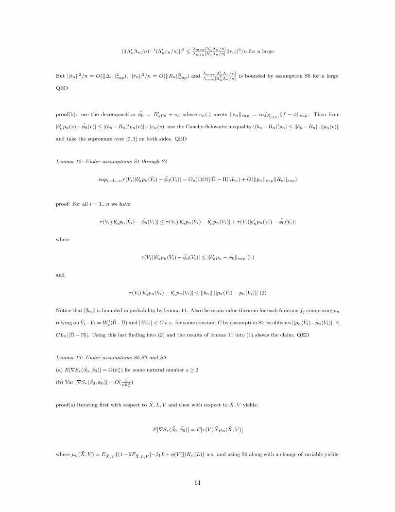
||(Λ′nΛn/n)−1(Λ′nrn/n)||2 ≤ λmax[Λ′nΛn/n]

λmin[Λ′nΛn/n]||rn||2/n for n large

But ||δn||2/n = O(||∆n||2sup), ||rn||2/n = O(||Rn||2sup) andλmax[Λ′nΛn/n]

λmin[Λ′nΛn/n]is bounded by assumption S5 for n large.

QED

proof(b): use the decomposition φ0 = B′npn + en where en(.) meets ||en||sup = infEρ(n)||f − φ||sup. Then from

|b′npn(v)− φ0(v)| ≤ |(bn−Bn)′pn(v)|+ |en(v)| use the Cauchy-Schwartz inequality |(bn−Bn)′pn| ≤ ||bn−Bn||.||pn(v)||

and take the supremum over [0, 1] on both sides. QED

Lemma 12: Under assumptions S1 through S5

supi=1...nτ(Vi)|b′npn(Vi)− φ0(Vi)| = Op(1)O(||Π−Π||.Ln) +O(||pn||sup||Rn||sup)

proof: For all i = 1...n we have:

τ(Vi)|b′npn(Vi)− φ0(Vi)| ≤ τ(Vi)|b′npn(Vi)− b′npn(Vi)|+ τ(Vi)|b′npn(Vi)− φ0(Vi)|

where

τ(Vi)|b′npn(Vi)− φ0(Vi)| ≤ ||b′npn − φ0||sup (1)

and

τ(Vi)|b′npn(Vi)− b′npn(Vi)| ≤ ||bn||.||pn(Vi)− pn(Vi)|| (2)

Notice that ||bn|| is bounded in probability by lemma 11. Also the mean value theorem for each function fj comprising pn

relying on Vi−Vi = W ′i (Π−Π) and ||Wi|| < C a.s. for some constant C by assumption S1 establishes ||pn(Vi)−pn(Vi)|| ≤

CLn||Π−Π||. Using this last finding into (2) and the results of lemma 11 into (1) shows the claim. QED

Lemma 13: Under assumptions S6,S7 and S9

(a) E[∇S∗(β0, φ0)] = O(hs∗) for some natural number s ≥ 2

(b) Var [∇S∗(β0, φ0)] = O( 1nh2∗

)

proof(a):Iterating first with respect to X, L, V and then with respect to X, V yields:

E[∇S∗(β0, φ0)] = E[τ(V )Xµn(X, V )]

where µn(X, V ) = EX,V (1− 2FX,L,V [−β1L+φ(V )])Kn(L) a.s. and using S6 along with a change of variable yields:

61

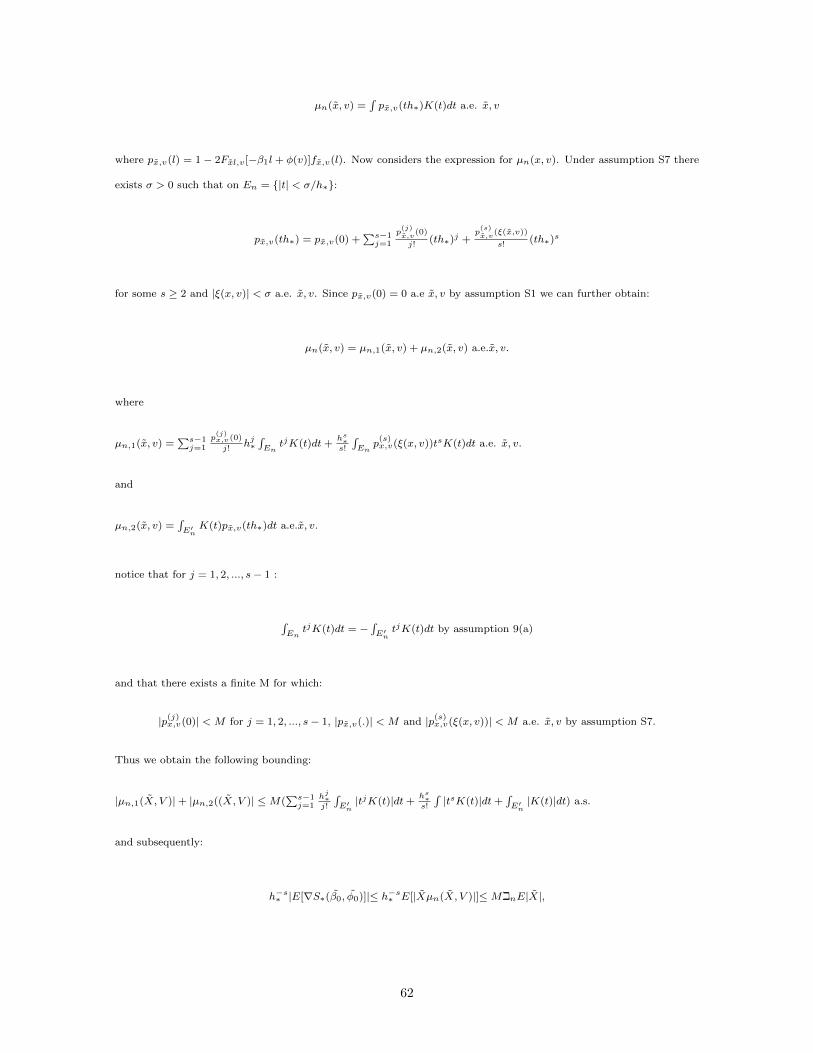
µn(x, v) =∫px,v(th∗)K(t)dt a.e. x, v

where px,v(l) = 1− 2Fxl,v [−β1l + φ(v)]fx,v(l). Now considers the expression for µn(x, v). Under assumption S7 there

exists σ > 0 such that on En = |t| < σ/h∗:

px,v(th∗) = px,v(0) +∑s−1j=1

p(j)x,v

(0)

j!(th∗)j +

p(s)x,v

(ξ(x,v))

s!(th∗)s

for some s ≥ 2 and |ξ(x, v)| < σ a.e. x, v. Since px,v(0) = 0 a.e x, v by assumption S1 we can further obtain:

µn(x, v) = µn,1(x, v) + µn,2(x, v) a.e.x, v.

where

µn,1(x, v) =∑s−1j=1

p(j)x,v(0)

j!hj∗

∫En

tjK(t)dt+hs∗s!

∫En

p(s)x,v(ξ(x, v))tsK(t)dt a.e. x, v.

and

µn,2(x, v) =∫E′n

K(t)px,v(th∗)dt a.e.x, v.

notice that for j = 1, 2, ..., s− 1 :

∫En

tjK(t)dt = −∫E′n

tjK(t)dt by assumption 9(a)

and that there exists a finite M for which:

|p(j)x,v(0)| < M for j = 1, 2, ..., s− 1, |px,v(.)| < M and |p(s)

x,v(ξ(x, v))| < M a.e. x, v by assumption S7.

Thus we obtain the following bounding:

|µn,1(X, V )|+ |µn,2((X, V )| ≤M(∑s−1j=1

hj∗j!

∫E′n|tjK(t)|dt+

hs∗s!

∫|tsK(t)|dt+

∫E′n|K(t)|dt) a.s.

and subsequently:

h−s∗ |E[∇S∗(β0, φ0)]|≤ h−s∗ E[|Xµn(X, V )|]≤MinE|X|,

62

where in =∑s−1j=1

hj−s∗j!

∫E′n|tjK(t)|dt+ 1

s!

∫|tsK(t)|dt+h−s∗

∫E′n|K(t)|dt. But in is a bounded sequence by assumption

S1,S9(a)and S9(e) while E|X| exists by assumption S1. QED

proof(b): This is immediate under the iid sampling assumption since 1nE[|X|2|Kn(L)|2] ≤

||K||2supnh2∗

E|X|2 where E|X|2

exists by assumption S1 and ||K||sup exists by S9(b). QED

Lemma 14: Under assumptions S6,S7 and S9

(a) lim E[HS∗(β0, φ0)] = Q as n →∞

(b) Var [HS∗(β0, φ0)] = O( 1nh4∗

)

proof(a): By the same approach as in lemma 12 we get:

E[HS∗(β0, φ0)] = E[τ(V )XX′An(X, V )]

where

An(X, V ) = EX,V (1− 2FX,L,V [−β1L+ φ(V )])K(1)n (L) a.s.,

and invoking assumptions S7,S9(e) and a similar argument as in lemma 3 one can easily derive:

lim An(X, V ) = −p(1)

X,V(0) a.s.,

where pX,V (.) is as defined in lemma 12. The claim follows by Dominated convergence since E|XX′| exists by assumption

S1. QED

proof(b): This is immediate using the same bounding principle as in proof(b) of lemma 12 invoking instead the existence

of both ||K(1)||sup (by assumption S9(b)) and E[XX′XX′] (by assumption S1). QED

Proposition 1

proof: under assumption 4(b), gX,`(v) is well defined and S(θ) exists uniformly over RK . For any θ ∈ RK such that

||∆|| > 0 where ∆ = θ − θ0 we have:

S(θ0)− S(θ) = E[1[|X′∆| > 0](d(`)− d(`+X′∆))gX,`(v)]

Using iterated expectation yields:

S(θ0)− S(θ) = E[1[|X′∆| > 0]EX(d(`)− d(`+X′∆))gX,`(v)].

63

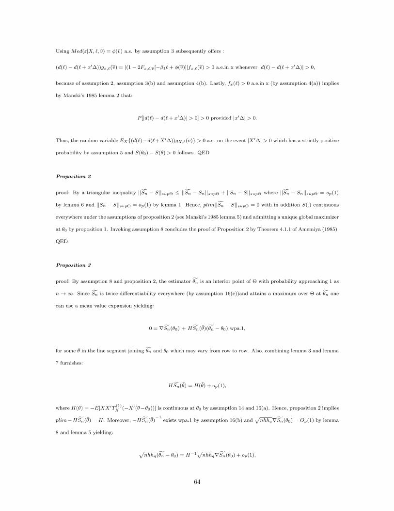
Using Med(ε|X, `, v) = φ(v) a.s. by assumption 3 subsequently offers :

(d(`)− d(`+ x′∆))gx,`(v) = |(1− 2Fx,`,v [−β1`+ φ(v)]|fx,`(v) > 0 a.e.in x whenever |d(`)− d(`+ x′∆)| > 0,

because of assumption 2, assumption 3(b) and assumption 4(b). Lastly, fx(`) > 0 a.e.in x (by assumption 4(a)) implies

by Manski’s 1985 lemma 2 that:

P [|d(`)− d(`+ x′∆)| > 0] > 0 provided |x′∆| > 0.

Thus, the random variable EX(d(`)−d(`+X′∆))gX,`(v) > 0 a.s. on the event |X′∆| > 0 which has a strictly positive

probability by assumption 5 and S(θ0)− S(θ) > 0 follows. QED

Proposition 2

proof: By a triangular inequality ||Sn − S||supΘ ≤ ||Sn − Sn||supΘ + ||Sn − S||supΘ where ||Sn − Sn||supΘ = op(1)

by lemma 6 and ||Sn − S||supΘ = op(1) by lemma 1. Hence, plim||Sn − S||supΘ = 0 with in addition S(.) continuous

everywhere under the assumptions of proposition 2 (see Manski’s 1985 lemma 5) and admitting a unique global maximizer

at θ0 by proposition 1. Invoking assumption 8 concludes the proof of Proposition 2 by Theorem 4.1.1 of Amemiya (1985).

QED

Proposition 3

proof: By assumption 8 and proposition 2, the estimator θn is an interior point of Θ with probability approaching 1 as

n→∞. Since Sn is twice differentiability everywhere (by assumption 16(e))and attains a maximum over Θ at θn one

can use a mean value expansion yielding:

0 = ∇Sn(θ0) + HSn(θ)(θn − θ0) wpa.1,

for some θ in the line segment joining θn and θ0 which may vary from row to row. Also, combining lemma 3 and lemma

7 furnishes:

HSn(θ) = H(θ) + op(1),

where H(θ) = −E[XX′T(1)X (−X′(θ−θ0))] is continuous at θ0 by assumption 14 and 16(a). Hence, proposition 2 implies

plim−HSn(θ) = H. Moreover, −HSn(θ)−1

exists wpa.1 by assumption 16(b) and√nhhq∇Sn(θ0) = Op(1) by lemma

8 and lemma 5 yielding:

√nhhq(θn − θ0) = H−1

√nhhq∇Sn(θ0) + op(1),

64

where lemma 8 further yields:

√nhhq(θn − θ0) = H−1

√nhhq∇Sn(θ0) + op(1),

and proposition 2 follows from lemma 5. QED

Proposition 4

proof: The first part of the proposition is straightforward by simply combining lemma 3 and lemma 7. For the second

part, introducing some notation is convenient. Given a bandwidth pair σ∗ ≡ (h∗ = hγ1 , hq∗ = hγ2q ) define:

Σn(σ∗) = 1nh∗hq∗

∑ni=1XiX

′i|K(

Ci+X′iθ0

h∗)|2|k(Vi−v

hq∗)|2

Hence we have:

Σn = Σn − Σn(σ∗) + Σn(σ∗)

Using the same approach as in lemma 5, it is rapid to show lim E[Σn(σ∗)] = Σ as long as both h∗ and hq∗ converge

to 0 as n approaches infinity. Furthermore, using a similar bounding method as in lemma 7 one has Var [Σn(σ∗)] ≤

M1M2nh∗hq∗

∫|K|4

∫|k|4 where M1 and M2 are finite constants. Hence, if both

∫|K|4 and

∫|k|4 exist, one needs the

additional condition that lim nh∗hq∗ = ∞ to ensure plim Σn(σ∗) = Σ. Under the assumption of proposition 4 this

condition holds for h and hq by assumption 13 and lim nh4h4q = ∞ by assumption 17 so a fortiori for hγ1 and hγ2q .

Secondly, we have:

Σn − Σn(σ∗) = 1nh∗hq∗

∑ni=1 XiX

′i[|Ki|2|ki|2 − |Ki|2|ki|2]

where

Ki = K(Ci+X

′iθ0

h∗)

and

ki = k( Vi−vhq∗

)

while Ki,ki are their counterparts when both θ0 and Π are used instead. Doing some simplifications with a triangular

inequality and using the fact that k(.) and K(.) are bounded functions yields:

|Σn − Σn(σ∗)| ≤ R1,n +R2,n,

where

R1,n = 2(||k||sup)(||K||sup)2 1nh∗hq∗

∑ni=1 |XiX′i||ki − ki|,

65

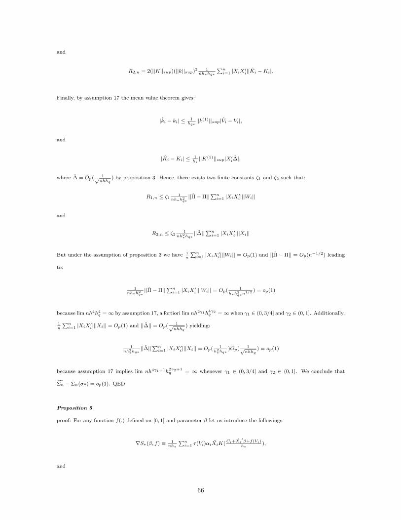
and

R2,n = 2(||K||sup)(||k||sup)2 1nh∗hq∗

∑ni=1 |XiX′i||Ki −Ki|.

Finally, by assumption 17 the mean value theorem gives:

|ki − ki| ≤ 1hq∗||k(1)||sup|Vi − Vi|,

and

|Ki −Ki| ≤ 1h∗||K(1)||sup|X′i∆|,

where ∆ = Op( 1√nhhq

) by proposition 3. Hence, there exists two finite constants ζ1 and ζ2 such that:

R1,n ≤ ζ1 1nh∗h2

q∗||Π−Π||

∑ni=1 |XiX′i|||Wi||

and

R2,n ≤ ζ2 1nh2∗hq∗

||∆||∑ni=1 |XiX′i|||Xi||

But under the assumption of proposition 3 we have 1n

∑ni=1 |XiX′i|||Wi|| = Op(1) and ||Π − Π|| = Op(n−1/2) leading

to:

1nh∗h2

q∗||Π−Π||

∑ni=1 |XiX′i|||Wi|| = Op( 1

h∗h2q∗n

1/2 ) = op(1)

because lim nh4h4q =∞ by assumption 17, a fortiori lim nh2γ1h4γ2

q =∞ when γ1 ∈ (0, 3/4] and γ2 ∈ (0, 1]. Additionally,

1n

∑ni=1 |XiX′i|||Xi|| = Op(1) and ||∆|| = Op( 1√

nhhq) yielding:

1nh2∗hq∗

||∆||∑ni=1 |XiX′i|||Xi|| = Op( 1

h2∗hq∗

)Op( 1√nhhq

) = op(1)

because assumption 17 implies lim nh4γ1+1h2γ2+1q = ∞ whenever γ1 ∈ (0, 3/4] and γ2 ∈ (0, 1]. We conclude that

Σn − Σn(σ∗) = op(1). QED

Proposition 5

proof: For any function f(.) defined on [0, 1] and parameter β let us introduce the followings:

∇S∗(β, f) ≡ 1nh∗

∑ni=1 τ(Vi)αiXiK(

Ci+Xi′β+f(Vi)h∗

),

and

66

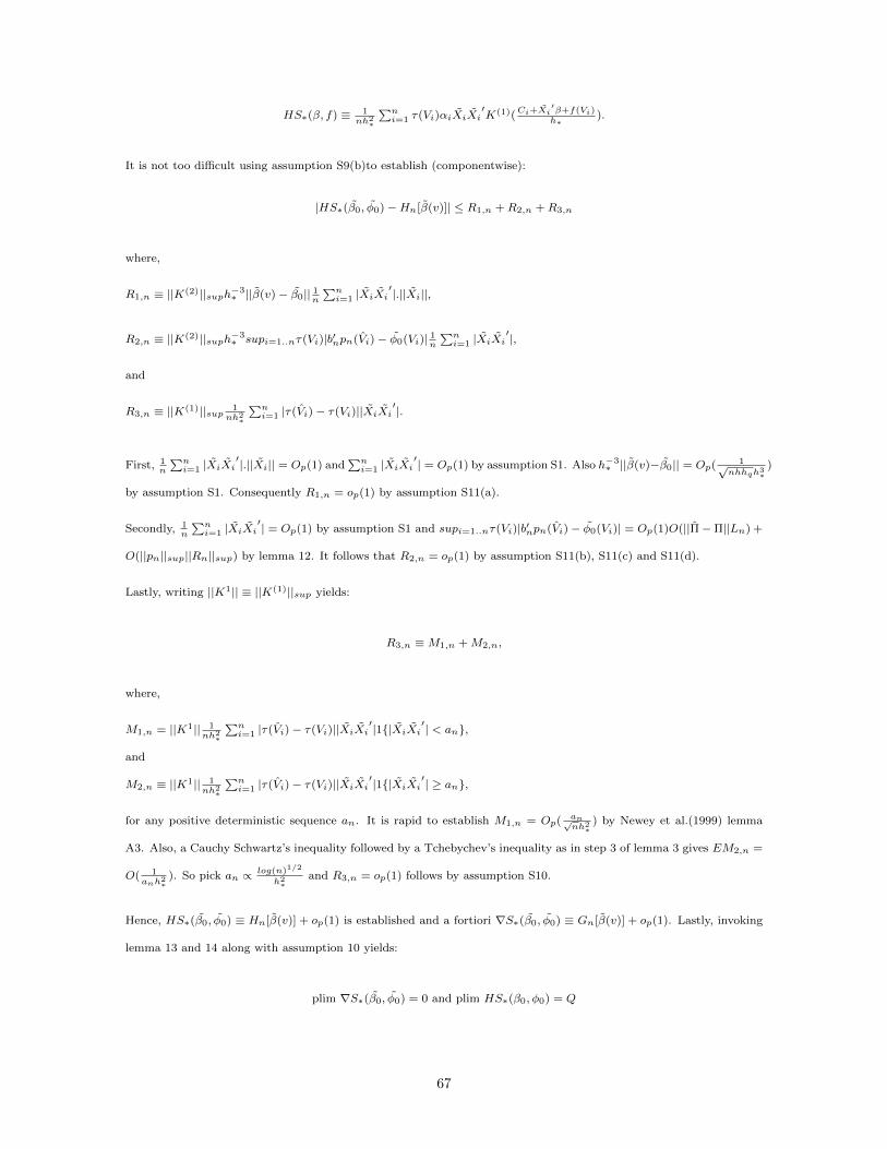
HS∗(β, f) ≡ 1nh2∗

∑ni=1 τ(Vi)αiXiXi

′K(1)(

Ci+Xi′β+f(Vi)h∗

).

It is not too difficult using assumption S9(b)to establish (componentwise):

|HS∗(β0, φ0)−Hn[β(v)]| ≤ R1,n +R2,n +R3,n

where,

R1,n ≡ ||K(2)||suph−3∗ ||β(v)− β0|| 1n

∑ni=1 |XiXi

′|.||Xi||,

R2,n ≡ ||K(2)||suph−3∗ supi=1..nτ(Vi)|b′npn(Vi)− φ0(Vi)| 1n

∑ni=1 |XiXi

′|,

and

R3,n ≡ ||K(1)||sup 1nh2∗

∑ni=1 |τ(Vi)− τ(Vi)||XiXi

′|.

First, 1n

∑ni=1 |XiXi

′|.||Xi|| = Op(1) and∑ni=1 |XiXi

′| = Op(1) by assumption S1. Also h−3∗ ||β(v)−β0|| = Op( 1√

nhhqh3∗

)

by assumption S1. Consequently R1,n = op(1) by assumption S11(a).

Secondly, 1n

∑ni=1 |XiXi

′| = Op(1) by assumption S1 and supi=1..nτ(Vi)|b′npn(Vi)− φ0(Vi)| = Op(1)O(||Π−Π||Ln) +

O(||pn||sup||Rn||sup) by lemma 12. It follows that R2,n = op(1) by assumption S11(b), S11(c) and S11(d).

Lastly, writing ||K1|| ≡ ||K(1)||sup yields:

R3,n ≡M1,n +M2,n,

where,

M1,n = ||K1|| 1nh2∗

∑ni=1 |τ(Vi)− τ(Vi)||XiXi

′|1|XiXi′| < an,

and

M2,n ≡ ||K1|| 1nh2∗

∑ni=1 |τ(Vi)− τ(Vi)||XiXi

′|1|XiXi′| ≥ an,

for any positive deterministic sequence an. It is rapid to establish M1,n = Op( an√nh2∗

) by Newey et al.(1999) lemma

A3. Also, a Cauchy Schwartz’s inequality followed by a Tchebychev’s inequality as in step 3 of lemma 3 gives EM2,n =

O( 1anh2∗

). So pick an ∝ log(n)1/2

h2∗

and R3,n = op(1) follows by assumption S10.

Hence, HS∗(β0, φ0) ≡ Hn[β(v)] + op(1) is established and a fortiori ∇S∗(β0, φ0) ≡ Gn[β(v)] + op(1). Lastly, invoking

lemma 13 and 14 along with assumption 10 yields:

plim ∇S∗(β0, φ0) = 0 and plim HS∗(β0, φ0) = Q

67

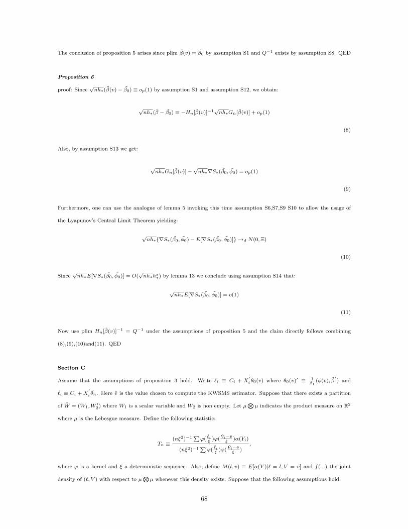
The conclusion of proposition 5 arises since plim β(v) = β0 by assumption S1 and Q−1 exists by assumption S8. QED

Proposition 6

proof: Since√nh∗(β(v)− β0) ≡ op(1) by assumption S1 and assumption S12, we obtain:

√nh∗(β − β0) ≡ −Hn[β(v)]−1

√nh∗Gn[β(v)] + op(1)

(8)

Also, by assumption S13 we get:

√nh∗Gn[β(v)]−

√nh∗∇S∗(β0, φ0) = op(1)

(9)

Furthermore, one can use the analogue of lemma 5 invoking this time assumption S6,S7,S9 S10 to allow the usage of

the Lyapunov’s Central Limit Theorem yielding:

√nh∗∇S∗(β0, φ0)− E[∇S∗(β0, φ0)] →d N(0,Ξ)

(10)

Since√nh∗E[∇S∗(β0, φ0)] = O(

√nh∗hs∗) by lemma 13 we conclude using assumption S14 that:

√nh∗E[∇S∗(β0, φ0)] = o(1)

(11)

Now use plim Hn[β(v)]−1 = Q−1 under the assumptions of proposition 5 and the claim directly follows combining

(8),(9),(10)and(11). QED

Section C

Assume that the assumptions of proposition 3 hold. Write `i ≡ Ci + X′iθ0(v) where θ0(v)′ ≡ 1

β1(φ(v), β

′) and

ˆi ≡ Ci + X

′i θn. Here v is the value chosen to compute the KWSMS estimator. Suppose that there exists a partition

of W = (W1,W ′2) where W1 is a scalar variable and W2 is non empty. Let µ⊗µ indicates the product measure on R2

where µ is the Lebesgue measure. Define the following statistic:

Tn ≡(nξ2)−1

∑ϕ(

ˆiξ

)ϕ( Vi−vξ

)α(Yi)

(nξ2)−1∑ϕ(

ˆiξ

)ϕ( Vi−vξ

),

where ϕ is a kernel and ξ a deterministic sequence. Also, define M(l, v) ≡ E[α(Y )|` = l, V = v] and f(.,.) the joint

density of (`, V ) with respect to µ⊗µ whenever this density exists. Suppose that the following assumptions hold:

68

C1. ∂M(l, v)\∂l and ∂M(l, v)\∂v exist and are continuous in some open neighborhood of (0, v). Also, ∂2M(l, v)\∂2l,

∂2M(l, v)\∂2v and ∂2M(l, v)\∂l∂v exist in some open neighborhood of (0, v).

C2. ϕ is a strictly positive kernel belonging to K2 and meets the same conditions as K in assumption 16.

C3. ξn is a strictly positive sequence of real numbers satisfying ξ ∝ n−ω for some ω ∈ (sup1/10; a(1 + η), 1/5) where

a and η are the bandwidths parameters selected to compute the KWSMS estimator as defined on page 28.

C4. The cdf of (`, V ) is absolutely continuous with respect to µ⊗µ, its density at (l, v)=(0, v) exists and is strictly

positive. Also, there exists some open neighborhood of (0, v) where ∂f(l, v)\∂l, ∂f(l, v)\∂v, ∂2f(l, v)\∂2l, ∂2f(l, v)\∂2v

and ∂2f(l, v)\∂l∂v exist and are continuous with |∂2f(l, v)\∂2l| < M , |∂2f(l, v)\∂2v| < M and |∂2f(l, v)\∂l∂v| < M

for some M <∞.

C5. The (cdf of) C|x, v, w is absolutely continuous with respect to the Lebesgue measure a.e in x, v, w and W1|x, w2 is

absolutely continuous with respect to the Lebesgue measure a.e in x, w2.

C6. (Define F [.|x, l, v, w] the cdf of ε|x, l, v, w. Also, write f(.|x, v, w) the density of `|x, v, w and f(.|x, l, w2) the density

of V |x, l, w2 whenever those densities exist.)

(i) As functions of l :

(ia)f(l|x, v, w) and F [−l|x, l, v, w] belong to C2∞(M) for some M <∞ a.e in x,v,w.

(ib)f(l|x,w) and F [−l|x, l,−λ′w + v, w] belong to C2∞(M) for some M < ∞ a.e in x,w for all λ parameter having

the dimension of W . Furthermore, f(−λ′w + v|x, l, w2) belongs to C2∞(M) for some M < ∞ a.e in x,w2 for all λ

parameter having the dimension of W .

(ii) As functions of v :

(iia) F [−l|x, l, v, w] belongs to C2∞(M) for some M < ∞ a.e in x,l,w. Also, f(v|x, l, w2) belongs to C2

∞(M) for some

M <∞ a.e in x,l,w2

(iib) F [λ′x|x,−λ′x, v, w] and f(−λ′x|x, v, w) belong to C2∞(M) for some M <∞ a.e in x,w for all λ parameter having

the dimension of X. Also, f(v|x,w2) belongs to C2∞(M) for some M < ∞ a.e in x,w2 for all λ parameter having the

dimension of X.

then under Ho: Med(ε|X, v) = Med(ε|v) a.s.,

√nξ2Tn →d N (0, f(0, v)−1(

∫|ϕ|2)2),

and,

(nξ2)−1∑ϕ(

ˆiξ

)ϕ( Vi−vξ

)→p f(0, v).

69

proof: The structure of this proof is analogous to that provided in Horowtiz (1993), proposition 2. The only difference

deals with the number of variables conditioning Y and the presence of an additional nuisance term Π from the reduced

form. The test is based upon the fact that under Ho: Med(ε|X, v) = Med(ε|v) a.s one must have M(0, v) = 0. The

proof for the consistent estimator of f(0, v) is omitted since it stems directly from what is to follow.

For any ∆′ ≡ (∆′1,∆′2) where ∆1 is K × 1 and ∆2 is d× 1 introduce the following:

M(4) =(nξ2)−1

∑ϕ(

`i+X′i∆1

ξ)ϕ(

υi+W′i∆2

ξ)α(Yi)

(nξ2)−1∑ϕ(

`i+X′i∆1

ξ)ϕ(

υi+W′i∆2

ξ)

,

where υi ≡ Vi− v. The key is to notice that Tn = M(∆) where ∆′ = ((θ−θ0(v))′, (Π− Π)′). Applying Theorem 3.5-3.6

of Pagan and Ullah (1999) using assumptions C1 through C4 yields:

√nξ2M(0)−M(0, v)→d N (0, f(0, v)−1(

∫|ϕ|2)2).

Also, using a Taylor’s expansion furnishes:

M(∆) = M(0) + ∂M∂∆|′∆

∆

where plim ∆ = 0 by the assumptions of proposition 3. Writing a the numerator of M and b its denominator gives:

∂M∂∆

= b−2( ∂a∂∆

b− a ∂b∂∆

).

Under C2 and C6 one can apply lemma 2 as in lemma 3 to derive plim ∂a∂∆

=lim E ∂a∂∆

< ∞ and plim ∂b∂∆

=lim

E ∂b∂∆

< ∞ uniformly over a compact set of RK+q which contains 0. Likewise, by the same token as in lemma 4 using

a classic convolution argument invoking C1-C4 returns plim a=lim Ea < ∞ and plim b =lim Eb < ∞ uniformly over

a compact set of RK+q which contains 0. This establishes ∂M∂∆|∆ = Op(1) and

√nξ2M(∆) − M(0) = op(1) follows

because√nξ24 = op(1) by proposition 3 and C3 (i.e. ξ2/hhq = o(1)). QED

70