A Highway Travel Information System: Forecasting and ...

Final Report

FHWA/IN/JTRP-2000/8

A Highway Travel Information System: Forecasting and Publicizing Delays in the Indiana State Highway Network

By

Shu-Ling Yu Research Assistant

School of Civil Engineering Purdue University

Jon D. Fricker

Professor School of Civil Engineering

Purdue University

Joint Highway Research Program Project Number: C-36-54BBB

File Number: 3-3-54 SPR-2204

Conducted in Cooperation with the Indiana Department of Transportation

and the U.S. Department of Transportation Federal Highway Administration

The contents of this report reflect the views of the authors, who are responsible for the facts and the accuracy of the data presented herein. The contents do not necessarily reflect the official views or policies of the Indiana Department of Transportation or the Federal Highway Administration at the time of publication. This report does not constitute a standard, specification, or regulation.

Purdue University

West Lafayette, IN 47907 July 2004

55 7/04 JTRP-2000/8 INDOT Division of Research West Lafayette, IN 47906

INDOT Research

TECHNICAL Summary Technology Transfer and Project Implementation Information

TRB Subject Code 55: Traffic Flow Capacity and Measurement July 2004 Publication No.: FHWA/IN/JTRP-2000/8, SPR-2204 Final Report A Highway Travel Information System: Forecasting and

Publicizing Delays in the Indiana State Highway Network

Introduction The Highway Travel Information System (HTIS) is a long-term pre-trip information system providing information about expected events, such as road constructions. Recent research has focused on real-time and short-term pre-trip information system. Real-time and short-term pre-trip information systems are the most beneficial to those drivers already on the road or about to depart. The HTIS can be beneficial to both highway travelers and construction managers of roadway projects. Construction managers can use the HTIS to check the forecasted traffic impacts of a proposed construction project schedule. Travelers who have flexible schedules and would like to do pre-trip planning to avoid unnecessary delays can obtain knowledge of traffic conditions in the near future from the HTIS. An approach called Workzone Delay Equilibrium Estimation (WDEE) is used by the HTIS to predict traffic conditions as construction zones age. Two extreme values of link volumes are calculated based on two scenarios: “no information”, in which no drivers know about a

new road capacity reduction, and “complete information”, in which all drivers have adequate information about road construction zones. A relationship between link volumes and the age of a project has been hypothesized and applied to the two extreme cases to estimate link volumes during construction periods. Finally, expected delays on links under construction are estimated based on the estimated link volumes. The objectives of the HTIS are:

- To predict the delays on the major highways in Indiana that are caused by scheduled roadway projects for expected travel levels and patterns;

- To build a user-friendly interface providing individuals and institutions with easy access to this travel information system;

- To provide INDOT with a method to review (and possibly revise) its construction project schedules;

To establish standard procedures to operate, maintain and update the HTIS.

Findings The delays in relation to the age of construction are estimated using the approach of Workzone Delay Equilibrium Estimation (WDEE) hypothesized for the HTIS. WDEE involves the following three steps: 1. Analysis for the “no information” scenario:

In the “no information” scenario, the traffic demands on each link with no construction and

at the beginning of road construction are treated the same. The “no information” link flows are estimated based on historical flows at the time before the workzone is added, using a simplified traffic volume forecasting technique developed for the HTIS. The travel delays for the “no information” case can be estimated by applying queueing theory using the “no information” link flows as arrival rates and workzone capacities as service rates.


2. Analysis for the “complete information” scenario:

In the “complete information” scenario, it is

assumed that drivers will divert to alternate routes rather than change their departure times to minimize delays. The travel between each O-D pair for a specific time period and day type is treated to be the same for both the “complete information” and “no information” scenarios. To simulate the “complete information” scenario, two analyses are involved – O-D estimation and traffic assignment. O-D estimation generates an O-D table based on the link flows for the “no information” case. Equilibrium traffic assignment is applied to the network with workzone capacities in place, using the O-D table obtained from O-D estimation. The travel delays for the “complete information” case can be estimated by applying queueing theory using the “complete information” link volumes as arrival rates and workzone capacities as service rates.

3. Estimation of delays during the construction

period The delay on a link is related to the traffic flow on the link. In queueing theory, it is assumed that delay occurs on a link when the traffic volume is greater than its capacity. When delay occurs, the delay on a link decreases as the link volume decreases. The volumes at a workzone are expected to decrease as construction proceeds and more drivers become aware of the construction. The traffic patterns during the construction period are determined by analyzing historical traffic data during construction periods. The relationship between the historical data and the age of construction can be applied to the links in workzones to obtain expected link volumes at any time during the construction period. The expected delays on each link can be estimated based on the expected link volumes.

Implementation The HTIS is divided into three subsystems for the purpose of meeting the needs of different groups of users. They are the modeling, project scheduling, and web access subsystems. The modeling and project scheduling subsystems are for management purposes and the web access subsystem is for use by the traveling public. 1. Modeling subsystem

The modeling subsystem is built using the Excel VBA and the TransCAD GISDK interfaces. The Excel VBA interface implements the simplified traffic volume forecasting technique proposed by HTIS. The TransCAD GISDK interface performs the analysis of the “no information” scenario, the “complete information” scenario, Workzone Delay Equilibrium Estimation (WDEE) during the transition construction period, delay estimation and delay database generation.

2. Project scheduling subsystem

The project scheduling subsystem is built using the TransCAD GISDK interface. There

are two major tasks for the project scheduling subsystem. The first one is to manage construction schedule databases. The second one is to assist project scheduling personnel in determining scheduling strategies that avoid excessive delays to traffic by providing functions to adjust project starting date, end date, and lane closure strategies in terms of workzone capacities.

3. Web access subsystem

The web access subsystem is built on several scripting languages, including Hyper Text Markup Language (HTML), JavaScript, VB-script, and Active Server Pagers (ASP). The JavaScript and VB-script provide an interactive environment. Drivers may input their desired departure time and receive information about expected delays at workzones that are active during their proposed trips. Motorists can use the information to plan their trips up to two months in advance.


Contact For more information: Prof. Jon D. Fricker Principal Investigator School of Civil Engineering Purdue University West Lafayette IN 47907 Phone: (765) 494-2205 Fax: (765) 496-1105

Indiana Department of Transportation Division of Research 1205 Montgomery Street P.O. Box 2279 West Lafayette, IN 47906 Phone: (765) 463-1521 Fax: (765) 497-1665 Purdue University Joint Transportation Research Program School of Civil Engineering West Lafayette, IN 47907-1284 Phone: (765) 494-9310 Fax: (765) 496-1105

TECHNICAL REPORT STANDARD TITLE PAGE

1. Report No. 2. Government Accession No.

3. Recipient's Catalog No.

FHWA/IN/JTRP-2000/8

4. Title and Subtitle A Highway Traveler Information System: Forecasting and Publicizing Delays in the Indiana State Highway Network

5. Report Date July 2004

6. Performing Organization Code 7. Author(s) Shu-Ling Yu and Jon D. Fricker

8. Performing Organization Report No. FHWA/IN/JTRP-2000/8

9. Performing Organization Name and Address Joint Transportation Research Program 1284 Civil Engineering Building Purdue University West Lafayette, Indiana 47907-1284

10. Work Unit No.

11. Contract or Grant No.

SPR-2204 12. Sponsoring Agency Name and Address Indiana Department of Transportation State Office Building 100 North Senate Avenue Indianapolis, IN 46204

13. Type of Report and Period Covered

Draft Final Report

14. Sponsoring Agency Code

15. Supplementary Notes Prepared in cooperation with the Indiana Department of Transportation and Federal Highway Administration. 16. Abstract

The Highway Travel Information System (HTIS) is a long-term pre-trip information system providing information about expected events, such as road construction. The HTIS can be beneficial to both highway travelers and roadway project schedulers. Project schedulers can use the HTIS to check the forecasted traffic impacts of a proposed construction project schedule. If the schedule would cause unacceptable delays, a scheduler can try new schedules to reduce the delay. Travelers who have flexible schedules and would like to do pre-trip planning can obtain knowledge of traffic conditions in the near future from HTIS to avoid unnecessary delays.

An approach called Workzone Delay Equilibrium Estimation (WDEE) is used by the HTIS to predict traffic conditions as construction zones age. Two extreme values of link volumes are calculated based on two scenarios: “no information”, in which no drivers know about a new road capacity reduction, and “complete information”, in which all drivers have adequate information about road construction zones. A relationship between link volumes and the age of a construction project has been hypothesized and applied to the two extreme cases to estimate link volumes during construction periods. Finally, the expected delays on links under construction are estimated based on the estimated link volumes.

The HTIS is divided into three subsystems for the purpose of meeting the needs of different groups of users. They are the modeling, project scheduling, and web access subsystems. The modeling and project scheduling subsystems are for management purposes and the web access subsystem is for use by the traveling public. The modeling subsystem is built using Excel VBA and TransCAD GISDK interfaces. The main function of the modeling subsystem is to model traffic conditions and generate a delay database. The project scheduling subsystem is built on the TransCAD GISDK interface. The major tasks for the project scheduling subsystem include schedule database management and assisting project scheduling. The web access subsystem is built on several scripting languages, including Hyper Text Markup Language (HTML), JavaScript, VB-script, and Active Server Pagers (ASP). With the web access subsystem, travelers may input their proposed departure times and receive information about expected delays at workzones that are expected to be active during their trips. Motorists can use the information to plan their trips up to two months in advance. 17. Key Words Highway Travel Information System (HTIS), pre-trip, work zone, delay, project scheduling.

18. Distribution Statement No restrictions. This document is available to the public through the National Technical Information Service, Springfield, VA 22161

19. Security Classif. (of this report)

Unclassified

20. Security Classif. (of this page)

Unclassified

21. No. of Pages

233

22. Price

Form DOT F 1700.7 (8-69)

Acknowledgments

The authors would like to thank the members of the Study Advisory Committee for

their helpful support. These persons are Mike Andrews, Rebecca Black, David Boruff,

Jay DuMontelle, Yi Jiang, Roger Manning, Wendall Meyer, Dean Munn, John Nagle,

Dan Shamo, Stephen Smith, Mike Wood, and Rick Yunker. Special thanks to Stephen

Smith and Dean Munn for providing modeling related reports, assisting collecting data

and loaning software; Roy Wasson and Geradine Lampley for providing ATR data;

Rick Yunker and John Nagle for furnishing data about construction schedules; David

Boruff for helping to find suitable construction projects; Dan Shamo for stimulating new

ideas; Richard Lively for clarifying web publishing issues; Yi Jiang for providing

reports related to workzone delay; Rebecca Black for assisting on growth factor related

issues.

iv

TABLE OF CONTENTS

Page

LIST OF TABLES............................................................................................................. vi LIST OF FIGURES .........................................................................................................viii 1. INTRODUCTION ........................................................................................................ 1

1.1 Problem Statement ............................................................................................... 2 1.2 Purposes and Objectives ...................................................................................... 3 1.3 Research Plan....................................................................................................... 4

2. LITERATURE REVIEW ............................................................................................. 9

2.1 Highway Information System.............................................................................. 9 2.2 Traffic Volume Forecasting............................................................................... 17 2.3 Workzone Delay Estimation .............................................................................. 22

3. DATA AVAILABLE.................................................................................................. 26

3.1 Network File ...................................................................................................... 26 3.2 Historical Link Volumes.................................................................................... 30

3.2.1 Automated Traffic Recorders (ATRs)........................................................... 30 3.2.2 County Flow Maps ........................................................................................ 31

3.3 Initial O-D Matrices........................................................................................... 31 3.4 Link Capacities .................................................................................................. 33

4. SOFTWARE APPRAISAL ........................................................................................ 41

4.1 Network Capacity .............................................................................................. 41 4.2 Capability on Traffic Assignment...................................................................... 42 4.3 Capability for O-D Estimation........................................................................... 43 4.4 User Interfaces ................................................................................................... 44 4.5 Effort to Build Inputs ......................................................................................... 46 4.6 Chapter Conclusions .......................................................................................... 47

v

Page

5. METHODOLOGY ..................................................................................................... 50 5.1 Framework ......................................................................................................... 50 5.2 Traffic Volume Forecasting............................................................................... 55 5.3 O-D Estimation .................................................................................................. 84 5.4 Traffic Assignment ............................................................................................ 88 5.5 Delay Estimation................................................................................................ 92

5.5.1 Estimating Upper and Lower Bounds for Delay ........................................... 94 5.5.2 Delay Refinement........................................................................................ 107

6. SYSTEM DEVELOPMENT .................................................................................... 161

6.1 Modeling Subsystem........................................................................................ 163 6.2 Project Scheduling Subsystem......................................................................... 169 6.3 Web Access Subsystem ................................................................................... 171 6.4 System Maintenance ........................................................................................ 172

7. SUMMARY AND FINAL COMMENTS................................................................ 186

7.1 Summary .......................................................................................................... 186 7.2 Final Comments ............................................................................................... 190

LIST OF REFERENCES................................................................................................ 193 APPENDIX HIGHWAY TRAVEL INFORMATION SYSTEM USER’S GUIDE .... 197

A.1 Excel VBA Interface........................................................................................ 198 A.2 TransCAD GISDK Interface............................................................................ 203

A.2.1 Modeling Subsystem ................................................................................... 204 A.2.1.1 Link Volume Forecasting................................................................... 204 A.2.1.2 Delay Verifications............................................................................. 209 A.2.1.3 Delay Database Generation and Conversion...................................... 210

A.2.2 Project Scheduling Menu ............................................................................ 211 A.3 Web Access Interface ...................................................................................... 217

vi

LIST OF TABLES

Table Page

4.1 Comparisons of TRANPLAN and TransCAD as the selected traffic demand software for the highway travel information system.............................................. 49

5.1 rs of Spearman Rank Correlation Test on ATR Station 2400 (November 3 ~

November 9, 1997)............................................................................................... 116 5.2 48 periods ahead forecasts at base period 160 and 24 periods ahead updated

forecasts at base period 184 (November 1997) .................................................... 117 5.3(a) Raw data for two ATR stations belonging to the urban interstate highway

road class (11/1/97~11/7/97)............................................................................... 118 5.3(b) Raw data for two ATR stations belonging to the urban interstate highway road

class (11/1/97~11/7/97) ........................................................................................ 119 5.4 Sum of hourly volumes for both directions and both stations.............................. 120 5.5 Peak period definitions and peak period factor calculations ................................ 121 5.6 Peak period definitions based on a single ATR station........................................ 122 5.7(a) Sum of volumes for each direction for days belonging to the same day type...... 123 5.7(b) Sum of volumes for each direction for days belonging to the same day type...... 124 5.8 Larger sum of volumes between two directions for days belonging to the

same day type ....................................................................................................... 125 5.9 Sum of larger sum of volumes between two directions for different day

types for all stations belonging to the same road class......................................... 126 5.10 Directionality calculation ..................................................................................... 127

vii

Table Page

5.11 Annual growth factors by functional class from 1990 to 1999 in Indiana State .. 128 5.12 Seasonal Adjustment Factors by Functional Class: 1994-1998 ........................... 129 5.13 Comparisons of annual growth factors based on the TMG with the ones

adopted by INDOT............................................................................................... 130 5.14 Stability analysis on the number of iterations in UE and SUE assignment

models .................................................................................................................. 131 5.15 Workzone capacity formula ................................................................................. 132 5.16 Comparison of measured travel time with calculated values ............................... 133

viii

LIST OF FIGURES

Figure Page

1.1 The relationship between link volumes and construction schedules........................ 8 3.1(a) Locations of ATR stations in Indiana (old system)................................................ 35 3.1(b) Locations of ATR stations in Indiana (new system) .............................................. 36 3.2 Malfunction occurred between November 13 and November 17 in

Westbound of ATR Station 1400 in 1997 .............................................................. 37 3.3 Excerpted ADTs in the “ADTVOL” field of a TransCAD network file................ 38 3.4 The process for generating initial O-D matrices .................................................... 39 3.5 Example link capacities for levels of service A to E (CapA ~ CapE) in

TransCAD network file .......................................................................................... 40 5.1 Research framework............................................................................................. 134 5.2(a) Northbound traffic patterns for normal days at station 2400 (November 1997).. 135 5.2(b) Southbound traffic patterns for normal days at station 2400 (November 1997).. 135 5.3(a) Northbound traffic patterns for the weeks before, during, and after

Thanksgiving Holiday at station 2400 (November 1997) .................................... 136 5.3(b) Southbound traffic patterns for the weeks before, during, and after

Thanksgiving Holiday at station 2400 (November 1997) .................................... 137 5.4 Northbound traffic patterns for Indy500 car racing event at station 2400

(May 1997) ........................................................................................................... 138 5.5 The first 160 weekday hourly volumes at ATR station 2400 in November

1997 ...................................................................................................................... 139

ix

Figure Page

5.6 Autocorrelation functions of the original series ................................................... 140 5.7 Autocorrelation functions of (1-B24)Zt ................................................................. 141 5.8 ACFs of the residuals of model (1,0,0)(1,1,1)24 ................................................... 142 5.9 ACFs of the residuals of model (1,0,125)(1,1,2)24 ................................................ 143 5.10 48-period-ahead forecasts of hourly traffic volumes at base period 160

and 24-periods-ahead updated forecasts of hourly traffic volumes at base period 184 (November 1997) ....................................................................... 144

5.11 Definition of bad data of high directionality ........................................................ 145 5.12 A typical queueing diagram ................................................................................. 146 5.13 Probability distribution of actual workzone capacity........................................... 147 5.14 A queueing diagram for situations when the AM-peak period is not followed

immediately by the PM-peak period (Tb1 ≤ t < Te1) ............................................. 148 5.15 A queueing diagram for situations when the AM-peak period is not followed

immediately by the PM-peak period (Te1 ≤ t < Tq1 and t+1 < Tq1) ...................... 149 5.16 A queueing diagram for situations when the AM-peak period is not followed

immediately by the PM-peak period (Te1 ≤ t < Tq1 and t+1 ≥ Tq1) ...................... 150 5.17 Queueing diagrams for situations when the PM-peak period comes

immediately after the AM-peak period ................................................................ 151 5.18 Field map of traffic survey on 5/9/99................................................................... 152 5.19 Field map of traffic survey on 6/20/99................................................................. 153 5.20 Queueing diagram for the first survey.................................................................. 154 5.21 Field map of traffic survey on 4/26/2000 through 5/9/2000 ................................ 155 5.22 Comparison of the demands from survey in 2000 and the historical volumes in

1996 ...................................................................................................................... 156 5.23 Comparison of the demands from survey in 2000 and the historical volumes

in 1996 (excluding weekends).............................................................................. 157

x

Figure Page

5.24 Difference between the demands from survey on the second week and on the first week .............................................................................................................. 158

5.25 A hypothesized relationship between the volume on workzone link and

the age of construction using a logistic function.................................................. 159 5.26 Logistic curves for two different percentages of uninformed travelers ............... 160 6.1 Relationships among three subsystems of HTIS.................................................. 181 6.2 Framework of the modeling subsystem................................................................ 182 6.3 Flowchart of the Excel VBA interface.................................................................. 183 6.4 Flowchart of the modeling subsystem’s TransCAD GISDK interface ................ 184 6.5 Time span definitions for traffic assignment........................................................ 185 Appendix Figure Page

A.1 Relationship of HTIS users’ interfaces ................................................................ 220 A.2 Framework of the Excel VBA interface............................................................... 221 A.3 Excel VBA introduction menu for the modeling subsystem................................ 222 A.4 Excel VBA main menu for modeling subsystem ................................................. 223 A.5 Open ATR files from the Excel VBA main menu ............................................... 224 A.6 An example ATR file in federal format (*.fed).................................................... 225 A.7 Special days input menu in the Excel VBA interface .......................................... 226 A.8 Definitions of peak periods for different day types and road classes................... 227 A.9 The output file of the peak period factors from the Excel VBA interface ........... 228 A.10 The output file of MADTs from the Excel VBA interface .................................. 229 A.11 Framework of the TransCAD GISDK interface................................................... 230 A.12 Screen capture for entering the TransCAD GISDK interface for HTIS .............. 231

xi

Appendix Figure Page

A.13 Main menu of the TransCAD GISDK interface................................................... 232 A.14 Input menu for TransCAD GISDK interface in modeling subsystem ................. 233 A.15 A map file in TrnsCAD map format (*.map) ....................................................... 234 A.16 An existing hourly volume file in dBase IV format (*.dbf) ................................. 235 A.17 An O-D matrix file in TransCAD matrix format (*.mtx)..................................... 236 A.18 Main menu for delay verification for TransCAD GISDK interface in

modeling subsystem ............................................................................................. 237 A.19 Output of delay verification for upper bound analysis only................................. 238 A.20 The output of delay verification for both upper bound and lower bound

analyses ................................................................................................................ 239 A.21 The dialog box for inputting the file name for delay database............................. 240 A.22 Dialog box for creating a new Access database ................................................... 241 A.23 Dialog box for importing a dBaseIV database ..................................................... 242 A.24 An example delay database .................................................................................. 243 A.25 Input menu for TransCAD GISDK interface in project scheduling subsystem ... 244 A.26 Schedule management menu for TransCAD GISDK interface in project

scheduling subsystem........................................................................................... 245 A.27 The existing records in the scheduling database are shown in a new table

and on the map ..................................................................................................... 246 A.28 Scheduling evaluation menu in project scheduling subsystem ............................ 247 A.29 The total delay of a specific period of time.......................................................... 248 A.30 Framework of the web access interface ............................................................... 249 A.31 Users’ interface for travel information access subsystem .................................... 250 A.32 Output screen for travel information access subsystem ....................................... 251

1

1. INTRODUCTION

As traffic congestion worsens (The CQ Researcher, 1999), many highway users are

eager for information to plan and adjust their trips to avoid unnecessary delays. To

improve traffic conditions, advanced traveler information systems (ATIS) are being

developed using different methodologies. ATIS focus mainly on providing real-time

information such as incident-induced delays. Real-time information systems are the most

beneficial to those travelers on the road. For travelers who have not yet started their trips,

have flexible schedules and can change their departure times, knowledge of traffic

conditions in the near future would be valuable. The travelers could avoid unnecessary

delays by scheduling trips departures at non-congested times or by planning beforehand

to travel on routes with less or no predicted delays. Therefore, this research proposes a

highway travel information system (HTIS) for long-term pre-trip purposes, permitting

highway users to improve their travel time, and assisting road construction managers in

revising schedules to avoid (if possible) restricted capacity during high traffic demand

periods.

Travel information can be presented in a variety of formats. Some information, such

as scheduled construction, scheduled events, levels of congestion, detour information,

and weather conditions, may be provided either during a trip or before departure, while

others such as incidents can be provided only during the trip.

2

The time at which information is provided affects the decisions of both highway users

and road construction managers. Highway users may use information about scheduled

events to determine their departure time and use real-time information to decide to

whether reroute while driving. Construction managers, on the other hand, require

information about forecasted high demands of traffic to schedule construction projects in

order to avoid causing additional delays.

The effectiveness of a travel information system depends on its accuracy, ease of use

and ease of maintenance. Accuracy and ease of use can win the trust of the system users.

Ease of maintenance makes the information system maintainers’ jobs easier and prolongs

the life of the system. It is the goal of the system developers to build a travel information

system with all of the above features.

Therefore, the main purpose of the HTIS is to establish an accurate, user-friendly and

easy-to-maintain pre-trip travel information system to meet the needs of highway users,

construction managers and system maintainers.

1.1 Problem Statements

Some problems may confront several parties in the absence of an appropriate travel

information system.

A. Highway users

Excessive delay may occur if drivers have incomplete information about scheduled or

existing reductions in roadway capacity. Drivers can benefit from information provided

during their trips. They can also plan and adjust their trips if relevant information is

provided before a trip is made. Drivers may use real-time information to avoid a traffic

3

jam, or use information about scheduled events before their departures to avoid the most

congested periods.

B. Road construction managers

Sometimes, scheduled construction coincides with periods of high traffic demand.

Highway construction is one of the major causes of delay to traffic flow. If construction

managers can reschedule projects to avoid seasons, days, or hours of high traffic demand,

the negative impacts of highway construction on traffic flow can be reduced. If delay

costs to society are compared against the possible increases in construction costs, the

rescheduling of projects may be justified.

1.2 Purposes and Objectives

One of the problems that the maintainers of some travel information systems have is

how to estimate the diversion rate from a route with road construction to alternate routes.

The diversion rate depends on many factors, such as the amount and nature of travel

information understood by the driver, the traffic conditions on major routes relative to

those on alternate routes, drivers’ preferences and weather conditions. For example,

some drivers may choose to divert on sunny days while stay on the original routes on

snowy days. Among these factors, the amount and nature of travel information

understood by the driver have the greatest influence on the diversion rate. Diversion

rates vary as construction projects go on. At the beginning of a road project, few drivers

may have adequate information with which to choose alternate routes. The diversion

rates may be small at first. As the road construction continues, more drivers become

aware of the capacity reductions, and consider alternate routes. The diversion rates

4

become larger. Because diversion rates have this dynamic characteristic, the actual

volumes on the original routes become hard to predict.

The dynamic characteristic of diversion rates as construction projects go on is

addressed in this research. Once this dynamic characteristic of diversion rates can be

successfully addressed, the delays caused by scheduled roadway projects can be

predicted. With the delay information, highway users may schedule their trips to avoid

unnecessary delays. Project schedulers may use the delay information to evaluate the

impacts on construction projects on traffic and make necessary adjustments.

The objectives of this research are listed as follows:

(1) To predict the delays on the major highways in Indiana State caused by scheduled

roadway projects for expected travel levels and patterns;

(2) To build a user-friendly interface providing individuals and institutions with easy

access to this travel information system;

(3) To provide INDOT with a method to review (and possibly revise) its construction

project schedules;

(4) To establish standard procedures for information updates using the newest available

data.

1.3 Research Plan

This research introduces an approach called Workzone Delay Equilibrium Estimation

(WDEE) to predict traffic conditions as construction ages. WDEE takes into

consideration that a certain percentage of uniformed travelers may not make informed

decisions, and fins a new “steady state” when the existence of the workzone has become

5

widely known. By applying a hypothetical relationship between link volumes and the

age of construction, the link volume at any time during the period before the system

reaches a new “steady state” can be estimated.

The flow rate entering a workzone can fall between two extreme values. These

extreme values correspond to two scenarios:

• The “no information”scenario, in which no drivers know about a new road

capacity reduction,

• The “complete information” scenario, in which all drivers have adequate

information about road construction zones.

To simulate the “no information” scenario, the link flows are estimated based on

historical flows at the time before the workzone is added. The link flows for the “no

information” case are assumed to be the same as that for a diversion rate of zero. The

travel delays for the “no information” case can be estimated based on the link flows for

the “no information” case and workzone capacities. To simulate the “complete

information” scenario, two analyses are involved, O-D estimation and traffic assignment.

O-D estimation is applied to generate an O-D table based on the link flows for the “no

information” case. Equilibrium traffic assignment is applied to the network with

workzone capacities in place based on the O-D table obtained from O-D estimation.

Neither scenarios will be strictly true, but they form the upper and lower bounds on travel

delay during the road construction period.

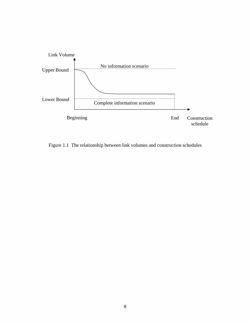
A relationship between link volumes and construction schedules is hypothesized and

applied to estimate link volumes during construction periods (Figure 1.1). As road

construction proceeds, diversion rates and link volumes gradually shift from the results of

6

the “no information” scenario toward the results of the “complete information” scenario.

The link volume for any time during construction periods can be estimated by applying

the hypothetical relationship to the two extreme values of link volumes.

Finally, the expected delays on each link are estimated based on the estimated link

volumes. With WDEE, the expected delays are linked to construction schedules. The

changes of the link volumes related to construction schedules can therefore be addressed

without having to predict diversion rates from the main route.

The major tasks of this research include:

(1) Collect and process historical traffic data: Find the traffic patterns associated with

some scheduled events and holidays to forecast the demands on the roadway links

within Indiana.

(2) Estimate statewide trip tables: Apply O-D estimation to estimate statewide trip tables

from forecasted demands on links within the Indiana State highway network.

(3) Perform traffic assignment: Apply equilibrium traffic assignment to simulate the

“complete information” scenario in which all drivers have adequate information about

road construction zones.

(4) Estimate delays: Generate delay using a formula based on queueing theory.

(5) Refine delay estimates: Generate rules to depict dynamic changes of traffic conditions

due to different levels of driver knowledge about roadway capacity reductions and

alternate routes.

(6) Verify and feedback: Conduct traffic surveys to verify the estimated delays. Receive

feedback from initial users and system maintainers. Modify the system

correspondingly.

7

(7) Build user interfaces to disseminate traffic information.

(8) Propose standard procedures for system maintenance.

8

Figure 1.1 The relationship between link volumes and construction schedules

Upper Bound

End Beginning Construction schedule

Link Volume

Lower Bound Complete information scenario

No information scenario

9

2. LITERATURE REVIEW

This chapter reviews past studies on three important topics related to the HTIS –

highway information systems, traffic volume forecasting methods and workzone delay

estimation. Section 2.1 reviews past studies of highway information systems. Previous

research about travel information systems can be categorized into three parts based on the

time at which information is provided – real-time information systems, short-term pre-

trip information systems, and long-term pre-trip information systems. The characteristics

and development of these three information systems are summarized.

Section 2.2 presents several traffic volume forecasting methods proposed in the past.

Not only various models and techniques applied to traffic forecast are reviewed, the

difficulties of forecasting traffic volumes in this research are also brought up.

Finally, a review of workzone delay estimation is given in Section 2.3, in which four

main approaches used to estimate workzone delay are introduced to readers. Their pros

and cons are discussed so that an appropriate approach for the HTIS is suggested.

2.1 Highway Information System

The current information systems can be divided into three groups – real-time, short-

term pre-trip and long-term pre-trip -information systems according to the time

information is provided. Real-time information systems provide travelers information

10

during driving, short-term pre-trip information systems provide information shortly

before departure (normally within one day), and long-term pre-trip information systems

provide information one day or more before departure. Real-time and short-term pre-trip

information systems are the most suitable for disseminating information about

unexpected events such as incidents, while long-term pre-trip information systems are

more suitable for informing drivers of expected events such as roadway construction.

The following discusses related research on real-time and short-term pre-trip information

systems, and long-term pre-trip information systems.

A. Real-time and short-term pre-trip information systems

Recent research on real-time and short-term pre-trip information systems has focused

on developing advanced traveler information systems (ATIS). ATIS are an integral

component of Intelligent Transportation Systems (ITS). The main objective of ATIS is to

provide travelers with dynamic route guidance and real-time information via different

media, such as in-vehicle route guidance systems, cellular telephones, cable television,

information kiosks and the Internet. The evolution of ATIS started from the one-way

communication systems, such as variable message signs (VMS) and highway advisory

radio (HAR) (Adler and Blue, 1998). In order to provide individual travel assistance, a

wide range of new technologies has been applied, such as real-time traffic surveillance

and control systems, electronic route guidance systems (ERGS) and in-vehicle route

guidance systems (IVRGS). These new technologies enable users to interact with ATIS

and provide individualized path search and dynamic route guidance. Despite of the

above evolutions, the development of ATIS is still in progress.

11

The effects of information provided by ATIS on travelers’ behavior have been

discussed by several researchers. Because ATIS are not well developed, the assessments

of the effects of information on travelers’ behavior are based on existing information

about dissemination media or simulation results. Polydoropoulou et al. (1994)

categorized these studies into two groups – revealed preference approach and stated

preference approach.

The revealed preference approach analyzes drivers’ behavior in real-life situations on

the basis of respondents’ reports, such as diary surveys and field observations. The

advantage of applying the revealed preference approach is that the resulting data are

based on travelers’ actual behavior. The disadvantage of this approach is that the costs of

collecting data are high. In addition, this approach may not be applied to new

technologies that have not been implemented, because no actual data are available.

Polydoropoulou et al. (1994) analyzed travelers’ behavior under the influence of traffic

information based on diary surveys. About 22% commuters received pre-trip traffic

information from radio and 5% from TV. Sixteen percent of commuters had their route

choice influenced by pre-trip information. It was concluded that a more reliable and

more frequently updated traffic information system than radio would gain driver

confidence and stimulate the acquisition of traffic information.

The stated preference approach obtains drivers’ impressions and reactions to

hypothetical scenarios through questionnaires, phone interviews and simulators. The

advantages of applying the stated preference approaches are that some environmental

factors are controllable and the costs of obtaining data are relatively lower than using the

revealed preference approach. However, the resulting data may not reflect travelers’

12

actual behavior. Additional verification is required. There are a lot of studies using the

stated preference approach. Some of them are discussed herein. According to Barfield et

al.’s (1991) study about the influence of information from radio, TV, variable message

sign (VMS) and phone on Seattle commuters’ behavior, about one third of commuters

would check information via TV before driving and over 60% of commuters would check

information via commercial radio stations before and during driving. Over 50% of

commuters have changed departure times or switched to alternate routes based on traffic

information. Only a small percentage of commuters have changed modes based on traffic

information. Khattak et al. (1995) evaluated the influence of radio traffic reports (RTR)

on Chicago commuters. Over 65% of commuters use RTR during driving and 40% use

RTR before driving. About 60% of commuters have changed departure times or

switched to alternate routes based on RTR. Khattak et al. (1999) conducted phone

interviews about the influence of information via radio, TV, phone on the behavior of

residents in San Francisco Bay Area. About 48% of residents listen to radio before

departure and 26% watch TV before departure. Eighty-two percent of automobile

noncommuters, 68% of automobile commuters, 66% of transit commuters, and 48% of

transit noncommuters are likely to adjust trips in response to travel information. Allen et

al. (1991) applied a self-designed simulator to analyze the responses of sampled drivers

to four congestion scenarios (11-minute delay – long-trip, 18-minute delay – long-trip,

30-minute delay – long-trip, and 30-minute delay – short-trip) and five in-vehicle

navigation systems (none, static map, dynamic map, advanced map and route guidance).

The results show that drivers diverted much earlier for both 30-minute delay conditions.

13

In addition, the more sophisticated navigation systems are, the higher the diversion

percentages are.

As can be seen from the studies with either the revealed preference or the stated

preference approaches, the effects of information on the choices regarding route and

departure times for each traveler are quite different. There are only a few models built to

describe the system performance resulting from the aggregation of individual behavior.

Arnott et al. (1991) proposed a simplified model for describing system performance due

to incidents on a two-route case. The effects of incidents were simulated by treating link

capacity as a stochastic variable. The probability of low capacity on a particular route

represents the significance of the incident that occurred on that route. The system

performances were divided into three scenarios based on the level of conveying

information – zero information, partial information and full information. With zero

information, travelers learn nothing about road capacities. Travelers’ choices of routes

and departure times are based on rational expectations and past experience. With full

information, travelers learn all about road capacities early enough for them to adjust their

routes and departure times, so that an equilibrium status can be reached. In equilibrium,

no one can reduce travel costs by changing route or departure time. It was concluded that

the expected costs per driver in the partial information scenario may be higher than in the

no information scenario due to the effect of “concentration”, which results from too many

drivers (but not all of them) following the route guidance.

The concept of the zero information, partial information and full information

scenarios in Arnott et al.’s model is the same as in the HTIS. The differences between

their model and the HTIS include:

14

(1) The stochastic link capacities in their model are for simulating the effects of

incidents. It is the effects of workzones that are the focus of the HTIS. Usually the

workzone capacities are treated as deterministic;

(2) Their model considered at most two links, while the HTIS addresses the entire road

network of Indiana;

(3) The effect of “concentration” happens only when too many travelers (but not all of

them) follow the same route, which is suggested by a route guidance system. The

HTIS deals with workzone information instead of recommending a specific route for

travelers to follow. Therefore, the effect of “concentration” is not discussed in the

HTIS.

The effects of information disseminated via the World Wide Web (WWW) on

traveler behavior regarding route choices and departure time choices are yet to be

decided. The WWW has been widely used for disseminating different kinds of

information, such as news, weather and advertising. The formats of information that can

be disseminated via the web range form pure text and images to audio and video clips.

Several scripting languages such as Javascript, VB-script, Common Gateway Interface

(CGI) and Microsoft Active Server Pages (ASP) enable the WWW to interact with users

and provide personalized information according to users’ preferences. An example of a

multimedia-based highway information system (MMHIS) in geographic information

system (GIS) shell was shown in Wang and Elliott’s study (1996). The MMHIS has a

feature of dynamic displaying data with video frames upon a user’s request by clicking

on a location on the map. As computer devices continue to improve and the prices of

these devices continue to drop, the number of Internet users in the nation has reached 106

15

million, over 52 % of American adults (Sefton, 2000). In considering the WWW soon to

become one of the major media, the HTIS includes it as one of the media for

disseminating travel information.

B. Long-term pre-trip information systems

Little attention has been given to long-term pre-trip information systems. Recent

research has focused on the real-time and short-term pre-trip information systems. The

real-time and short-term pre-trip information systems, however, provide only information

at the time it is accessed, in order to meet the requirements of disseminating information

about unexpected events. The long-term pre-trip information systems, on the other hand,

can provide motorists with knowledge of traffic conditions about expected or planned

events several months in advance, depending on the characteristics of those events.

Travelers who are planning ahead and have flexible schedules may be able to reschedule

their trips. Drivers in traffic may adjust their routes according to the real-time information

to minimize expected delay. Drivers about to begin a trip who consult short-term pre-trip

information system may be able to reschedule their trips or modify their routes.

Previous studies on the effects of road construction (one of the most common planned

events) on traffic have diverted much attention toward the short-term effects resulting

from different traffic control strategies. Nemeth and Rouphail (1982) studied the

merging behavior in response to traffic control devices using the self-built microscopic

simulation model Freeway Construction (FREECON). Dudek et al. (1986) conducted

surveys on lane closures on 4-lane highways in Dallas, Texas and Oklahoma City,

Oklahoma, and studied the relationships between hourly volumes and user costs induced

by workzones. Zhang et al. (1989) applied the simulation model FREQ10PC to assess

16

the different effects of traffic control strategies on traffic at the Oakland Bay Bridge in

San Francisco, California, and the impacts of nighttime lane closures on the traffic on I-

80 northeast of the Oakland Bay Bridge. Robertson, Palumbo and Rice (1995) evaluated

the impacts of a workzone at Metropolitan Boulevard in Montreal on adjacent roads.

Boruff (1994) evaluated the impacts of the I70 reconstruction from I465 to the Belmont

Avenue overpass in Indianapolis, Indiana by calculating the percentage changes of total

traffic volumes on both the major route and the alternate route.

In the studies mentioned above, none explores day-to-day variations in traffic patterns

due to workzones during the transition time before an equilibrium state is reached. The

day-to-day variations in traffic patterns due to workzones were evaluated in Jha and

Sinha’s study (1996). Jha and Sinha applied a dynamic traffic simulator

(DYNASMART) to a test network with 10 zones, 50 nodes and 168 links, and simulated

the effects of different percentages of travelers who trust and follow the route guidance

on the system performance in terms of average travel time. Their study can be a good

starting point for studying the effects of long-term pre-trip information on traffic. Two

aspects in their study need to be further developed:

(1) The lane closure strategies considered are only full lane closures (closures of all lanes

on links under construction), which are not common for state highways or higher.

The most common lane closure strategies for Indiana highways are partial lane

closures, in which the traffic flow is maintained.

(2) The network used in their study is only a test network. The implementation of

DYNASMART on long-term events in real networks of a large scale such as the

Indiana network can be difficult, because complicated modeling skills are required.

17

The HTIS further explores day-to-day variations in traffic patterns due to workzones

during the transition time before an equilibrium state is reached in two ways:

(1) Consider both full lane closure and partial lane closure strategies.

(2) Verify the impacts of workzones on traffic using a real network.

2.2 Traffic Volume Forecasting

Previous research on traffic volume forecasting applied various techniques. Some of

the studies applied neural network models (Dougherty and Cobbett, 1997; and Yun et al.,

1998), while some used time series models (Voort, Dougherty and Watson, 1996) to

forecast traffic volumes. The comparisons of these two models with several other

techniques are shown in Kirby et al.’s study (1997) and Smith and Demetsky’s study

(1997).

Kirby et al. (1997) evaluated the accuracies of using upstream volumes to predict

downstream volumes based on three forecasting models – neural network models, time

series models and the ATHENA model, which is a short-term forecasting model

developed by Institut National pour la Recherche sur les Transports et leur Sécurité

(INRETS). The data at three stations located about 30 kilometers upstream from the

target station were used to forecast the volumes of the target station. It was concluded

that both the neural network and the time series models can get a good forecasting result.

The ATHENA model was evaluated to be better than both the neural network and the

time series models.

Smith and Demetsky (1997) reviewed the accuracies of forecasting results using four

models – historical average, time series, neural network and nonparametric regression

18

models. They also accessed the transferability of these models. The data used for

forecasting were two sets of historical data from two locations. The first set of data was

used to evaluate the accuracy of the results based on the four models. It was shown that

the nonparametric regression model outperforms the other methods. The neural network

model was the second, followed by the time series model third and the historical average

model last. The time series model was excluded from the evaluations of model

transferability because it does not allow missing data, a common situation in practice.

The remaining three models were further evaluated for their transferability using the

second set of data from a different location. The transferability of the neural network

model was evaluated by processing the second set of data without “retraining”, which

means the parameters generated based on the first set of data are used directly without

updates from the second set of data. The forecasting results showed the nonparametric

regression model still remains in first place. The results using the neural network model

without “retraining” are even worse than using the historical average model. The neural

network model was concluded to be not transferable.

The accuracy of the forecasting results from applying the time series model to the

data at the same location needs to be evaluated. The evaluation of the time series model

conducted in Kirby et al.’s (1997) study was based on the data 30 kilometers upstream

from the target location. In Smith and Demetsky’s (1997) study, the time series model

was excluded because it was unable to process nonconsecutive data. Although the

situation of missing data also occurs to the ATR data due to malfunctions of equipment, it

is still not difficult to find adequate ATR data for use of the time series model in this

HTIS study. Consequently, the time series model being unable to process

19

nonconsecutive data is not a problem for this research. The evaluation of the time series

model based on data at an ATR location in Indiana is performed in Section 5.2.

In addition to the accuracy of forecasting results and model transferability, the

selection of a suitable traffic volume forecasting technique for the HTIS also depends on

the availability of historical data and the time required performing traffic volume

forecasting on all links within Indiana.

(1) Availability of historical data: The historical hourly volumes are needed either for

use in building forecasting models or for directly forecasting volumes by transferring

models from other locations. Forecasting volumes by transferring models from other

locations may not need as much historical data as when building models “from

scratch.” The forecasting models themselves cannot forecast hourly volumes without

using any historical hourly volumes as a basis. Most of the links within the Indiana

do not have historical hourly volumes. The only historical data available for all links

within Indiana are the average daily traffic volumes (ADTs) on county flow maps.

The problem of insufficient historical volume data is explained in Section 3.2.

(2) Time required performing traffic volume forecasting on all links within the Indiana:

The existing Indiana highway network file in TransCAD format contains over 16,000

links, and the network file in TRANPLAN format contains over 1,100 links. The

traffic volume forecasting process needs to be repeated for each link within the

network because the demand for each link is required for the O-D estimation process

in the “complete information” scenario to generate the demand for each O-D pair. If

the time to process a single link is one minute, the time to process all links in the

TransCAD network file is over 260 hours, and the time to process all links in the

20

TRANPLAN network file is over 18 hours. Therefore, any forecasting technique that

requires over hours to process a single link is not practical for use in the HTIS.

In considering the above two reasons, advanced traffic volume forecasting models

such as nonparametric regression, time series and neural network techniques are not

appropriate for use in the HTIS. A simplified approach for traffic volume forecasting is

proposed for the HTIS by modifying the approach to adjust 48-hour counts taken on

sample sections to AADTs for the same base year in the Traffic Monitoring Guide

(TMG) (FHWA, 1995).

The TMG issued by the Federal Highway Administration (FHWA) provided a

simplified approach for estimating average adjustment factors for link volumes (monthly

factors, day-of-week factors and growth factors) for links of the same group for use in

adjusting daily volumes from short-term surveys to AADTs of the same base year. The

criterion for grouping links with similar traffic patterns is by classification of links. The

TMG suggests five groups – urban interstate highways, other urban highways, rural

interstate highways, other rural highways, and recreational highways. It is not the interest

of the HTIS to distinguish recreational highways from other highways. Therefore, only

the first four groups are used to group the ATR data. The data required for calculating

the average adjustment factors for link volumes include two sets of data that are routinely

collected: (1) hourly volumes collected from the Automated Traffic Recorders (ATRs),

which are loop detectors and weigh-in-motion devices used for collecting continuous

traffic data; and (2) the 48-hour counts taken on sample sections. The calculation process

involves three steps: (1) grouping ATR data based on road classes of links; (2)

calculating average factors for each group based on the ATR data of the same group; (3)

21

applying the average factors for each group to the 48-hour counts taken on sample

sections, which belong to the same group.

Because the AADTs in the base year 1995 are available in the TransCAD network

file, there is no need for AADT conversions. However, the AADTs in the TransCAD

network file are required to be converted to AADTs in current year. The average growth

factors are calculated following the process suggested in the TMG. The calculation

process for average growth factors is implemented in the HTIS (see Section 5.2).

The HTIS proposes a simplified traffic volume forecasting approach by modifying

the daily volumes adjustment procedure proposed in the TMG. This simplified approach

adopts the same grouping technique as in the TMG. The differences between this

approach and the TMG link volumes adjustment procedure are the required data and the

calculation process. The data required include the ATR data and the AADTs from the

TransCAD network file, which are converted from the data stored in the county flow

maps. The calculation process involves five steps:

(1) Grouping ATR data based on road classes of links;

(2) Calculating average growth factors for each group based on the ATR data of the same

group;

(3) Applying the growth factors for each group to the AADTs from the TransCAD

network file to obtain AADTs of current year;

(4) Calculating average peak period factors and directionality for each group based on the

ATR data of the same group; and

(5) Applying the peak period factors and directionality for each group to the AADTs of

current year to obtain hourly volumes for different peak periods.

22

The detailed calculation processes of this simplified traffic volume forecasting

approach and an example are shown in Section 5.2.

One of the advantages of this simplified approach is that it does not require historical

hourly volumes for all links. The only required historical data are historical hourly

volumes for ATR stations and historical daily volumes for all links stored in the

TransCAD network file. Unlike the existing traffic volume forecasting techniques, this

approach can be applied to all links, including those without historical hourly volumes.

In addition, the processing time of estimating hourly volumes for all links using this

simplified approach is over 90% shorter than using advanced traffic volume forecasting

techniques such as time series and neural network techniques.

2.3 Workzone Delay Estimation

Research on the impacts of highway workzones on traffic has used different ways to

quantify the effects. The most commonly used quantitative indices to evaluate the

impacts of workzones on traffic include, queueing lengths, workzone user costs,

workzone delays and total travel time.

Queueing lengths can be estimated in several ways, such as a deterministic queueing

approach, stochastic queueing methods, a shock wave approach and a coordinate

transformation time-depend technique. Dixon et al. (1998) compared the queueing length

estimation techniques of deterministic, shock wave, and coordination transformation with

an estimated field queue. Among the three techniques, the coordinate transformation

technique can produce the closest values to the estimated field queue. All of the three

techniques tend to underestimate the queue length. The use of queue length as an index

23

for evaluating the impacts of workzones may be sufficient for choosing better traffic

control strategies. However, queue length is not the way most drivers measure traffic

congestion; they do it in terms of time. Therefore, providing queue lengths as travel

information cannot efficiently assist travelers on trip planning.

The workzone user costs convert the effects of all impacts of workzones into money

values. The definitions of user costs at workzones vary in different studies. Memmott

and Dudek (1982) defined the total user costs at workzones using seven components: (1)

cost of delay, (2) delay cost of going through the workzone at reduced speed, (3) cost of

the speed-change cycle, (4) operating cost of the speed-change cycle before a queue is

present, (5) additional operating cost of the speed-change cycle when a queue is present,

(6) vehicle running cost before a queue is present, and (7) additional vehicle running cost

when a queue is present. Soares and Najafi (1998) divided workzone user costs into three

components – travel time delay costs, vehicle operating costs, and accident costs. The

advantage of using workzone user costs to evaluate the impacts of workzones is that it

includes money-related costs in addition to time-related costs. The use of workzone user

costs as travel information has the same problem as queueing lengths. The value of

workzone user costs is not meaningful to travelers as travel time and queueing delay.

Workzone delays and travel time – as opposed to queue lengths and workzone user

costs – provide direct information that travelers can use for trip decisions. Researchers

have adopted different approaches to estimate workzone delays and travel time.

Davies et al. (1981) proposed a model to estimate the delays in four different traffic

conditions – “free-flow”, “queue starts to form”, “diversion” and “diversionary route at

capacity.” In the “free-flow” condition, the link demand on the main route is less than its

24

capacity and there are only speed reductions through the workzone. In the “queue starts

to form” condition, the link demand on the main route is greater than the capacity and no

traffic has been diverted. In the “diversion” condition, the traffic starts to divert to the

alternate route. In the “diversionary route at capacity”, both the main route and the

alternate route have reached their capacities. Davies, Vincent and Jacoby’s study was to

estimate the impacts due to short-term construction, such as maintenance work.

Cassidy and Han (1993) proposed a model for estimating delays and queue lengths at

two-lane highway workzones. When one of the two lanes closed, traffic in both

directions needs to share the remaining open lane. This type of lane closure was called

“one-way traffic control” by the authors. Because the “one-way traffic control” is a

special case, the applications of Cassidy and Han’s study cannot be extended to other

types of lane closures.

Jiang (1999) reviewed the time-related costs defined in Memmott and Dudek’s study

and categorized total delays into four parts: (1) delay due to vehicle deceleration before

entering workzone, (2) delay due to reduced speed through workzone, (3) delay for

resuming freeway speed after exiting workzone, and (4) delay due to vehicle queues. The

total delays were further used to calculate workzone costs. The difference between

Jiang’s study and Memmott and Dudek’s study is the technique used to estimate delay.

Memmott and Dudek used queueing diagrams to calculate queueing delays, while Jiang

applied queueing theory. Both of these two studies focus on estimating the total

workzone user costs within a specified time period. The total delays calculated in these

two studies are with respect to all vehicles in the system during a certain period, instead

of for only those vehicles entering the system during the time period.

25

The HTIS applies queueing diagrams to model different combinations of arrival rates

and derives a general formula for these models. These models can be used to estimate

the total delays with respect to vehicles entering the system during a certain time period

and average workzone delay per vehicle. The queueing models used in the HTIS are

explained in Section 5.5.

26

3. DATA AVAILABLE

Several data are required to implement this highway travel information system. The

required data include a network file, historical link volumes, initial O-D matrices, and

workzone capacity constraints. This chapter explains the uses of these data, the formats

of the data obtained and the problems encountered if the data obtained cannot be used

directly.

3.1 Network File

A. The uses of network files

Network files are an important data resource for highway travel information systems.

They are large databases that contain information related to highway links, intersections

and interchanges such as geographical locations, road classifications, historical link

volumes, link lengths, speed limits, and link capacities.

Geographical locations of links and nodes are used to construct highway networks.

The geographical location of a highway link is defined by the coordinates of its two end

nodes. Road classifications of links are used for forecasting traffic patterns on links

during the link volume forecasting process. The traffic patterns for sample links of a road

class can represent those links of the same road class under the assumption that the traffic

patterns of the same road class are similar. Historical link volumes in the network files

27

are used as the basis for link volume forecasting. Link volumes in the near future are

forecasted based on historical link volumes. Link lengths and speed limits are used in

calculating travel time, which is for use in traffic assignment and O-D estimation. Link

capacities are for use in traffic assignment, O-D estimation and delay estimation.

B. The formats of the obtained data

There are two Indiana State network files available: one in TransCAD format and the

other in TRANPLAN format. The network file in TransCAD format was obtained from

Indiana Department of Transportation (INDOT). The TransCAD file includes all the

required data fields of all major highways in the Indiana state network and major arterials

in urban areas. Although the data for some of the highway links (such as link volumes)

are absent, only a few of the missing data are critical for our analysis.

The network file in TRANPLAN format is from the previous research project (Yang

and Fricker, 1996). Although the TRANPLAN file includes only some of the required

data for major highways in the Indiana State, it is capable of O-D estimation, using a

method called Fast Matrix Calibration. Detailed comparisons of TransCAD and

TRANPLAN in terms of record storage capacities and analysis capabilities appear in

Chapter 4.

To make use of the advantages of both TransCAD and TRANPLAN, the HTIS

attempted to convert the TransCAD network file to TRANPLAN formats, so as to use the

capability of Fast Matrix Calibration in TRANPLAN.

The original TransCAD network file contains 761 Traffic Analysis Zones (TAZs),

which include 667 township-level internal zones and 94 external zones. In considering

the degree of precision, the township-level TAZs may be too detailed for statewide trips.

28

The number of trips per day between most pairs of townships in the state is very small.

Because processing time increases as the number of TAZs increases, the HTIS planned to

combine the township-level TAZs into 134 TAZs, to include 92 county-level internal

zones and 42 external zones.

Several tasks were undertaken in the attempt:

(1) Internal TAZ centroid modifications: In combining the township-level internal TAZs

to county-level internal TAZs, the township centroids and their centroid connectors

need to be removed and new county centroids and centroid connectors need to be

added.

(2) External zones adjustments: The number of external zones needs to be reduced as the

number of internal TAZs decreases.

(3) O-D matrix modifications: The O-D matrix also needs to be modified

correspondingly to match the new identification numbers of the internal and external

TAZ centroids.

(4) Modified network verifications: The assigned link flows from the assignment of the

modified O-D matrix to the modified network are compared with the ones from the

assignment of the original O-D matrix to the original network. The differences

between the two assigned link flows should be within acceptable ranges.

(5) Network file conversion: The modified TransCAD network file is converted into the

formats of TRANPLAN.

C. The problems encountered

There were several problems encountered as the township-level TAZs were being

combined into county-sized TAZs.

29

(1) It requires considerable effort and time: Each task mentioned above requires

considerable effort and time. In addition, the first four tasks above may need to be

repeated if the results of verifications are not satisfactory.

(2) The verification results are not satisfactory: After investing a lot of effort and time,

the modified network file and O-D matrix were verified by performing traffic

assignment. The results showed a lot of zero-flow links, even on several major roads.

Possible causes of this problem include a complicated network system with few

centroids and inappropriate centroid connectors.

(3) There are limitations on data storage in TRANPLAN: The TransCAD database

contains large amounts of data that TRANPLAN could not handle. The version of

TRANPLAN we used limits the total node number to 10,000, which is less than the

15,223 links in the TransCAD network file.

In conclusion, the attempts to make use of the advantages of both TransCAD and

TRANPLAN network files were not successful. The large effort and time required, the

unsatisfactory verification results, and limitations on data storage in TRANPLAN make

the conversion of TransCAD network file to TRANPLAN format not worthwhile. An

alternative to building a complete network file is to use the existing network files in

TransCAD or TRANPLAN formats without conversions. Some modifications need to be

made when choosing to use either the TransCAD network file or the TRANPLAN

network file:

• TransCAD network file: Fill in missing data critical for analysis. No

simplifications are made.

30

• TRANPLAN network file: Add in required data fields and fill in data for all

highway links.

Detailed comparisons of TransCAD and TRANPLAN and the final selection of the

software to use appear in Chapter 4.

3.2 Historical Link Volumes

Historical link volumes are the data on the highway link volumes in the past. They

are used as the bases for link flow forecasting for specific time frames in the near future.

The forecasted values of link volumes for a specific time are treated as the demands on

the highway links at that time. These values are then used for delay estimations and O-D

matrix estimations.

The available historical link volumes are in the following two formats: Automated

Traffic Recorders (ATRs) and county flow maps.

3.2.1 Automated Traffic Recorders (ATRs)

ATRs are permanent stations that collect highway link volumes. There are two

sources of ATR data: Telemetry stations and Weigh In Motion (WIM) stations. There

are 58 Telemetry stations and 35 WIM stations within Indiana. Figure 3.1a shows the old

system used before 1999, and Figure 3.1b the new system used after 1999. Each station

records continuous hourly volumes when the detectors and equipment function well.

Some missing data due to malfunctions of the detectors and equipment are found in files

provided by INDOT (Figure 3.2).

31

3.2.2 County Flow Maps

County flow maps contain Annual Daily Traffic (ADT) volumes for each road

segment in the state highway network. The source of these data is 48-hour traffic counts

conducted by INDOT in each county every three to five years. The data in the county

flow map are not from the same time frame, because the counts are conducted over a 3-

to-5-year cycle. The problem with ADTs in different time frames has been solved by

INDOT by updating the ADTs in the county flow maps into the same time frame, such as

1995. The updated ADTs for 1995 are available in the “ADTVOL” field of the network

file (Figure 3.12).

In order to forecast the hourly traffic patterns of the links, the converted ADTs in

county flow maps need to be further converted into hourly format. The HTIS uses the

data of ATR stations as the basis for updating and forecasting link volumes in the county

flow map. The process is discussed in Section 5.2.

3.3 Initial O-D Matrices

A. The use of initial O-D matrices

Initial O-D matrices are tables recording the number of trips that occurred between

each pair of TAZs. The use of initial O-D matrices is one of the inputs of O-D

estimation, which generates estimated O-D matrices for specific time periods, based on

link volumes for those time periods. The estimated O-D matrices and link capacities with

workzone capacity constraints for specific time periods are then used in traffic

assignment to determine the link volumes under the scenario in which the road

construction locations are known by all road users.

32

B. The formats of initial O-D matrices

The initial O-D matrices obtained from INDOT are in two different formats: the daily

O-D table and multi-hour O-D tables that are in 3-hour and 18-hour periods. The daily

O-D table contains the number of trips between each pair of all TAZs in a weekday. The

source of the daily O-D tables is the result of using TransCAD’s O-D estimation feature

with a seed O-D table, which was developed with available Census, household travel

survey and socioeconomic data representative of travel condition in Indiana, and daily

link volumes contained in the network file as inputs (Cambridge Systematics Inc., 1998).

The multi-hour O-D tables provided through INDOT, on the other hand, contain only

the number of trips between each pair of internal TAZs for periods less than 24 hours,

including AM-peak, PM-peak, and off-peak periods. The AM-peak and the PM-peak

period each lasts three hours. The off-peak period, which includes the remaining periods

in a weekday, lasts eighteen hours. The sources of the multi-hour O-D tables are the

results of the daily O-D table applied by the time-of-day factors obtained from the

household travel survey data (Cambridge Systematric Inc., 1998).

The process of generating initial O-D matrices is shown in Figure 3.13.


As explained earlier, initial O-D matrices are one of the inputs for O-D estimation. In

order to perform O-D estimation, the time period formats of the initial O-D matrices

should match those of the link volumes, which are in hourly formats. Therefore, the

initial O-D matrices in both daily and multi-hour formats should be converted into hourly

formats.

33

In addition, the multi-hour O-D tables include only internal trips. The internal-

external and external-external trips are also required for O-D estimation. Therefore, these

tables are not suitable in the HTIS.

The daily O-D table, on the other hand, contains internal-internal, internal-external

and external-external trips. It can be used for O-D estimation after being converted to

hourly trip table. The daily to hourly conversion factor is obtained from the ATR data.

The process is discussed in Section 5.3.

3.4 Link Capacities

A. The uses of link capacities

The link capacities under prevailing roadway, traffic, and control conditions are

referred as normal capacities (HCM, 1997). The values of link capacities that change due

to the effects of road construction are referred as work zone capacities.

The uses of link capacities are for traffic assignment and delay estimation. Link

capacities are one of the inputs to traffic assignment. As explained in the use of initial O-

D matrices, the traffic assignment procedure applying workzone capacities to the links

under construction, and normal capacities to all other links, can determine the link

volumes under the scenario, in which the road construction locations are known to all

road users.

Workzone capacities are also one of the inputs for delay estimation due to road

construction. Delay estimation is discussed in Section 5.5.

34

B. The formats of road capacities

The normal capacities in the network file provided by INDOT are in two formats:

daily and hourly. The hourly normal capacities are in five different levels of service,

from level of service A to E. (See Figure 3.14.) The source of these normal capacities is

from a research project (Whitford and Opsuth, 1997) that calculated link capacities based

on the maximum flow that can be served under a specific level of service defined in the

Highway Capacity Manual (HCM, 1997).

Typical workzone hourly capacities have been established by Dudek and Richards’

study (1981). The detailed derivation of workzone capacities is discussed in Section 5.5.


The hourly normal capacities at level of service E for all lanes in the network file

provided by INDOT are used in the HTIS, because the volumes at level of service E are

usually treated as capacities. However, the hourly normal capacities in the INDOT file at

level of service E are two times higher than the values suggested in HCM (1997). A

temporary factor of 0.5 is applied to those values in the network file.

35

Figure 3.1(a) Locations of ATR stations in Indiana (old system)

36

Figure 3.1(b) Locations of ATR stations in Indiana (new system)

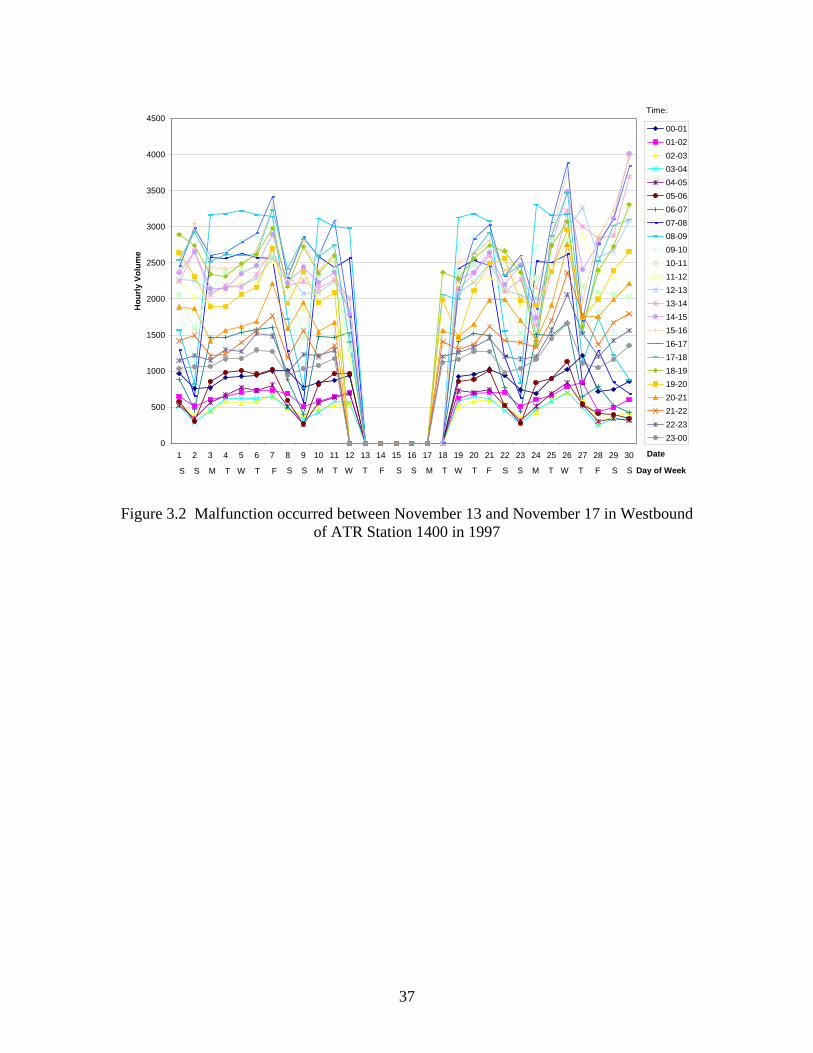
37

0

500

1000

1500

2000

2500

3000

3500

4000

4500

1 2 3 4 5 6 7 8 9 10 11 12 13 14 15 16 17 18 19 20 21 22 23 24 25 26 27 28 29 30 Date

Hou

rly V

olum

e00-0101-0202-0303-0404-0505-0606-0707-0808-0909-1010-1111-1212-1313-1414-1515-1616-1717-1818-1919-2020-2121-2222-2323-00

S S M T W T F S S M T W T F S S M T W T F S S M T W T F S S

Time:

Day of Week

Figure 3.2 Malfunction occurred between November 13 and November 17 in Westbound of ATR Station 1400 in 1997

38

Figure 3.3 Excerpted ADTs in the “ADTVOL” field of a TransCAD network file

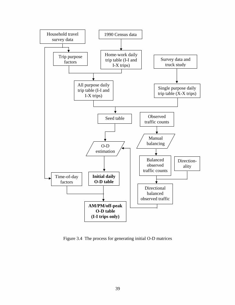
39

Figure 3.4 The process for generating initial O-D matrices

1990 Census data

Home-work daily trip table (I-I and

I-X trips)

Household travel survey data

Trip purpose factors

All purpose daily trip table (I-I and

I-X trips)

Survey data and truck study

Single purpose daily trip table (X-X trips)

O-D estimation

Seed table Observed traffic counts

Manual balancing

Balanced observed

traffic counts

Directional balanced

observed traffic

Initial daily O-D table

Time-of-day factors

AM/PM/off-peak O-D table

(I-I trips only)

Direction-ality

40

Figure 3.5 Example link capacities for levels of service A to E (CapA ~ CapE) in TransCAD network file

41

4. SOFTWARE APPRAISAL

Because the HTIS intends to use travel demand modeling procedures to forecast the

traffic conditions that could occur on specific links at specified times during the next

year, appropriate software tools are necessary to implement travel demand models. The

main object of this chapter is to compare two eligible software packages, TransCAD and

TRANPLAN, and to suggest an appropriate one for use in this research.

Two main features are considered in making the final decision: the problem-solving

functions provided by the package and the software efficiency in implementing the HTIS.

The first feature is evaluated by examining the package capabilities in three respects:

network capacity, traffic assignment, and O-D estimation. Then, two aspects regarding

software efficiency are taken into account: the user interface and the efforts required to

build inputs. These considered aspects are elaborated on separately in Sections 4.1 to 4.5.

In addition, Section 4.6 gives the conclusion for the discussion.

4.1 Network Capacity

A TRANPLAN study area is limited to 1,500 zones, 10,000 nodes, and node names

(expressed as numbers) no greater than 16,000. TransCAD, though not specifying its

limitations in the manual, is capable of dealing with networks beyond TRANPLAN’s

42

limitation on total node numbers and node names. The current TransCAD network file

for Indiana contains 761 zones and 15,223 nodes, with a maximum node name 311,326.

4.2 Capability on Traffic Assignment

Several methodologies of traffic assignments are developed based on different

optimal objectives, such as all-or-nothing, iterative capacity restraint, stochastic, user

equilibrium, stochastic user equilibrium, and system optimum, each of which is applied

for different purposes (Ortuzar and Willumsen, 1996). Among these traffic assignment

methods, user equilibrium and stochastic traffic assignments seemed to be most

appropriate for use in the HTIS.

User equilibrium traffic assignment is applied to simulate the “complete information”

scenario, in which all drivers have adequate information about road construction zones.

Under user equilibrium, no user may reduce his/her travel time by changing the route

taken. Therefore, user equilibrium can simulate the situation in which all drivers make

their optimal choices based on “complete information.”

Stochastic traffic assignment is well-suited to simulating users’ decisions when facing

two or more adjacent parallel routes. Even if one of the routes is superior to the other

route(s) in terms of saving time, some users may still choose another one. Unlike all-or-

nothing traffic assignment, none of the reasonable route alternates will have zero flow

when stochastic traffic assignment is used.

Both TRANPLAN and TransCAD provide the user equilibrium and stochastic

options for traffic assignment. Therefore, given the same network and the same

43

demands, both models can be tested to see if they produce network loadings that are

reasonable.

4.3 Capability for O-D Estimation

The O-D estimation techniques are needed in the HTIS to build statewide O-D

matrices based on observed traffic counts because most existing O-D tables from surveys

are prepared for local cities. Mathematically, the solutions (the O-D matrices) are usually

not unique, because the number of constraints (the number of traffic counts) is far fewer

than the number of unknown variables (the number of O-D pairs) (Ortuzar and

Willumsen, 1996).

The objective here is to find an O-D matrix that can produce a flow pattern that

adequately replicates the actual traffic situation. The more reliable the traffic counts are,

the more likely the resulting O-D table is to generate link volumes that are closer to the

“reliable” counts. The ability to constrain the O-D estimation procedure to match more

closely the more reliable data is a desirable trait.

TRANPLAN uses an add-on function called Fast Matrix Calibration (FMC) that can

adjust an existing origin-destination matrix to match given traffic flow constraints at

screenlines and zonal boundaries (BGC, 1993). FMC allows users to assign an elasticity

value to each screenline and zonal boundary. The elasticity governs the extent to which a

screenline and a zonal boundary can be adjusted relative to other screenlines and zone

boundaries. A higher elasticity of a screenline or a zonal boundary indicates that the

number of observed trips passing through the screenline or the boundary is trustworthier.

Therefore, the traffic assignment results based on the estimated O-D matrix should

44

produce the number of trips, which pass through the screenline close to the number of

trips observed. In this way, O-D matrices are adjusted according to the assigned elastic

boundary conditions. FMC can thus provide the user with more control over the results

of the O-D estimation.

TransCAD uses a Single Path Matrix Estimation Method (SPME) to estimate O-D

matrices from counted traffic by minimizing the average deviation between calculated

and counted traffic along the optimal path used by each zone pair. The optional path is

calculated by using All-or-Nothing assignment.

SPME solves the problem of unbalanced counted traffic that does not meet node

equilibrium by considering traffic counts as stochastic variables. However, because the

objective function in SPME is not to minimize the average deviation of the cells in the

estimated and old O-D matrices, the patterns of the estimated O-D matrices may be

completely different from the patterns of the old O-D matrices, which are usually

obtained from household surveys. The results of TransCAD’s O-D estimation are hard

for the user to control.

4.4 User Interfaces

User interfaces are an essential factor in the ease of use of highway travel information

systems. The users are those who responsible for building or operating this highway

information system, including system maintainers, INDOT personnel, and people

authorized to update it. The interfaces refer to the shells that accept human commands to

control the functions provided by the software. A friendly user interface can not only

45

effectively flatten the learning curve, but also shorten the time to build a new system and

make the maintenance easier.

TRANPLAN is a modularized transportation planning software package. Most tasks

in TRANPLAN require users to create control files and input files in text format. The

control files are executed through a console program under the DOS environment. Like a

computer language compiler, the console program always examines the inputs of control

files (and generate warning or error messages if there were any) before proceeds the

commands. For other tasks demanding a graphic interface to operate, TRANPLAN

provides an independent program called the Highway Network Information System

(HNIS), which generates and demonstrates geographic plots of network files. Separate

modules are also provided to control the database interface and to convert network data

from and to ARC/INFO GIS format.

The characteristic of modularizing separate functions in TRANPLAN makes it run

efficiently without including unnecessary functions in computer memory. However,

users are required to learn several different interfaces and to maintain files for each

interface. The learning curve in getting acquainted with several different interfaces is

relatively steep and file management is difficult. In addition, TRANPLAN does not

provide macro functions to create an independent interface for the travel information

system. All operations must be done through executing control files under the DOS

environment. The required of level of understanding of TRANPLAN itself is somewhat

high, which makes it not very user-friendly.

TransCAD is transportation-oriented Geographic Information System (GIS) software

that links the transportation database system to the graphical network. Users not only can

46

have a clear view of the graphical presentation of the network data, but also be able to

maintain and query network databases, and perform planning analysis procedures under a

single Graphic User Interface (GUI). Although TransCAD requires more computer

resources to run, because all functions under a single interface are included, it provides

macro functions to generate an independent interface for the travel information system.

Through the independent interface for the travel information system, users may perform

all required operations with only a basic understanding of how to operate TransCAD.

Therefore, the user interface of TransCAD is better than that of TRANPLAN for use in

the HTIS.

4.5 Effort to Build Inputs

The main effort of this research is to implement a highway travel information

system. The effort needed to build inputs to a network file for specific software should be

reasonable, rather than time-consuming. The best choice of a network file would be the

one that is ready for use. However, if the effort to build inputs for a network for specific

software is reasonable, the selection of software should be based on all factors, not just

the effort to build inputs.

As explained in Chapter 3, the TRANPLAN network file created in a previous

research project (Yang and Fricker, 1996) includes only some of the required data for

major highways in Indiana, such as link length, speeds, and capacities. Other data, such

as historical link traffic counts, road names, road classifications, county codes, and

numbers of lanes, are essential to travel information systems and would need to be added

to the TRANPLAN network file. The effort to add such inputs to the TRANPLAN

47

network file would be considerable. On the other hand, the TransCAD network file

obtained from INDOT includes all the required data fields, except for a few missing data

on several links. The only missing data that are essential to O-D estimation are historical

link traffic counts for some major highways. Only a little amount of time and effort are

needed to input those data into the TransCAD network file.

4.6 Chapter Conclusions

TRANPLAN and TransCAD were first chosen as the candidates for traffic demand

models for the HTIS because they both had statewide network files developed by

previous projects. These two candidates were evaluated based on the requirements of this

research. The comparisons of these two software packages are summarized in Table 4.1.

Both TRANPLAN and TransCAD provide sufficient options in traffic assignments

for use in the HTIS. Although TRANPLAN has the FMC function to provide better

control on the O-D estimation results, the lack of sufficient network capacity, a steep

learning curve, and the large effort required to build inputs for its network file make it

harder to be applied. TransCAD is superior because of its high network capacity, self-

built and friendly user interface, and ready-to-use network file. Although TransCAD

does not allow user control of the outcome of O-D estimation, the capabilities of

TransCAD are otherwise excellent for use in the HTIS.

Moreover, as discussed in Chapter 3, the available Indiana State network files are in

TransCAD format and in TRANPLAN format. To make use of the advantages of both

software packages, the HTIS first attempted to convert INDOT’s TransCAD network file

to TRANPLAN format. However, the conversion process could not be successfully

48

accomplished because of the large amount of effort and time required, the disappointing

verification results, and limitations on data storage in TRANPLAN. Therefore, the

options are to use either the TransCAD network file or the TRANPLAN network file, but

not to attempt a conversion. The first alternative is preferable because the network file in

TRANPLAN format is too simplified and it lacks of several essential information on

links.

Based on the comparative evaluation described in this chapter, TransCAD was

selected as the traffic demand model to be used in the HTIS.

49

Table 4.1 Comparisons of TRANPLAN and TransCAD as the selected traffic demand software for the highway travel information system

Capability TRANPLAN TransCAD

Network capacity

Traffic Assignment

O-D estimation O

User Interface

Efforts to build inputs

(note) : excellent O: good

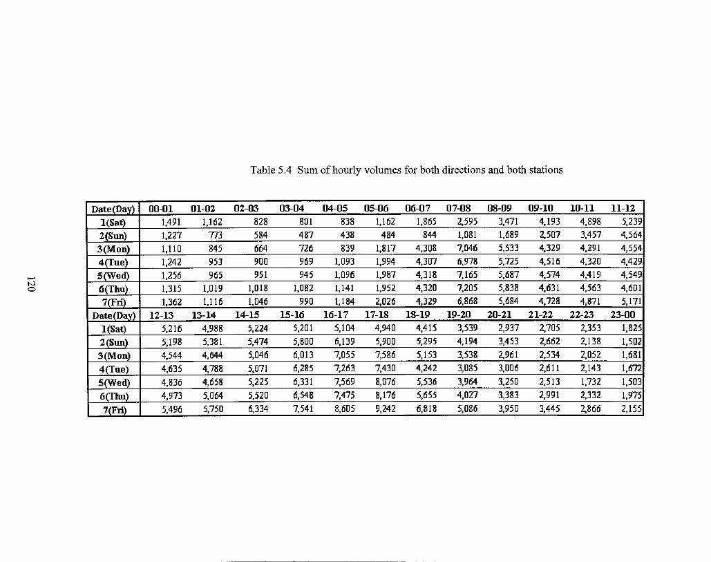
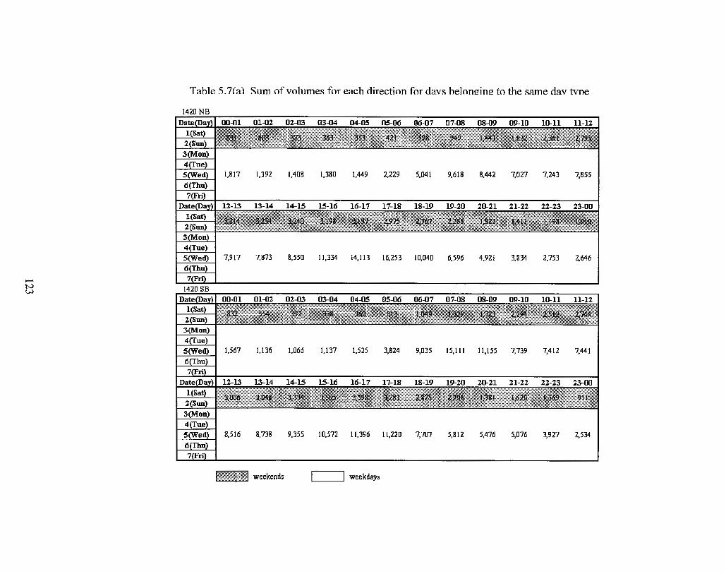
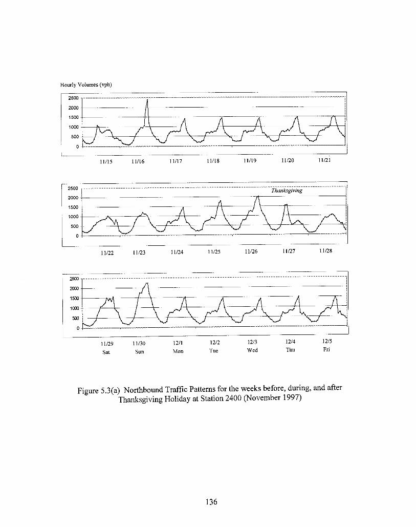
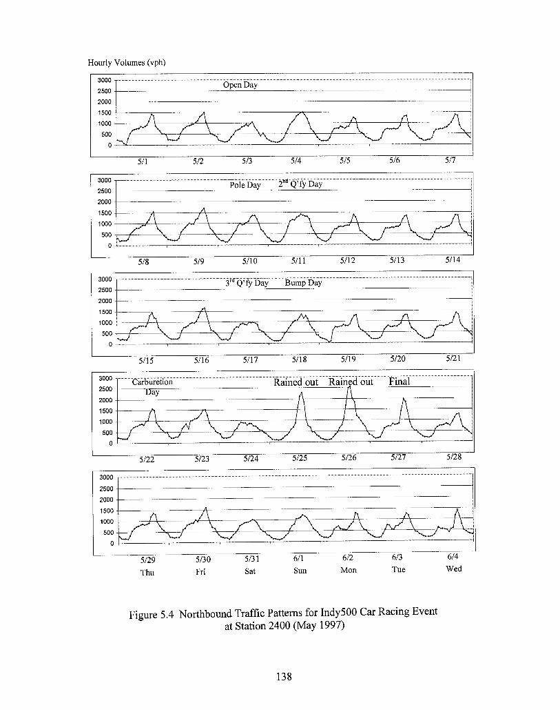
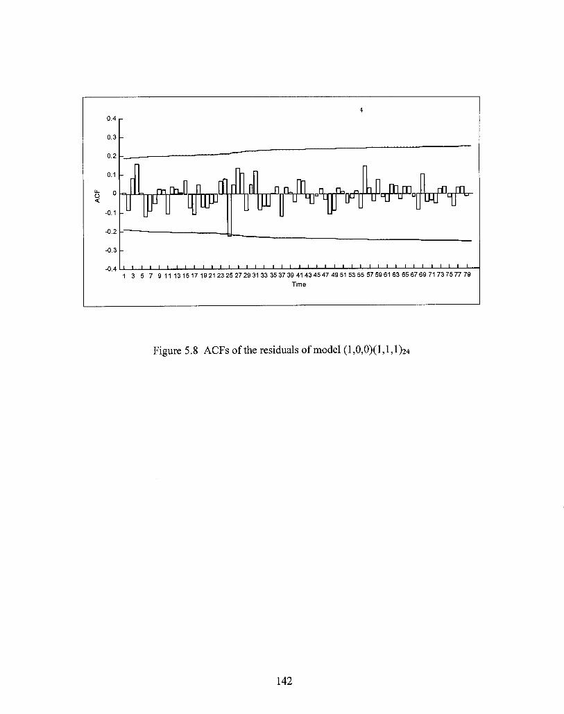
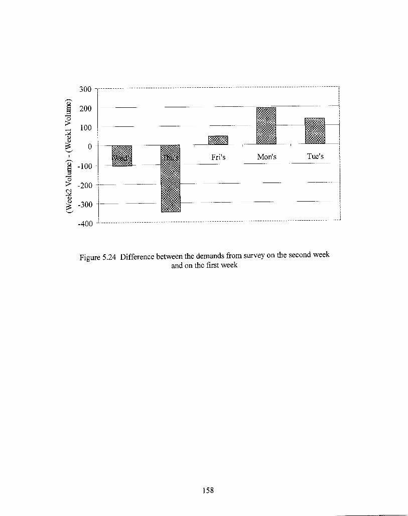
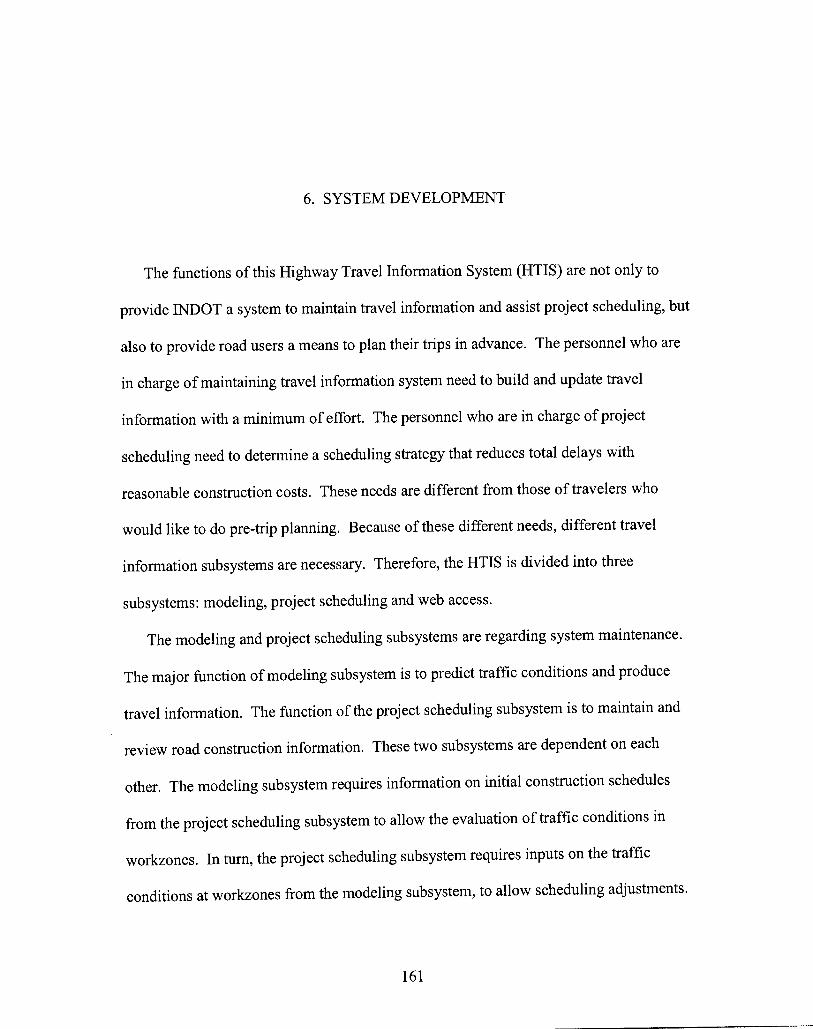
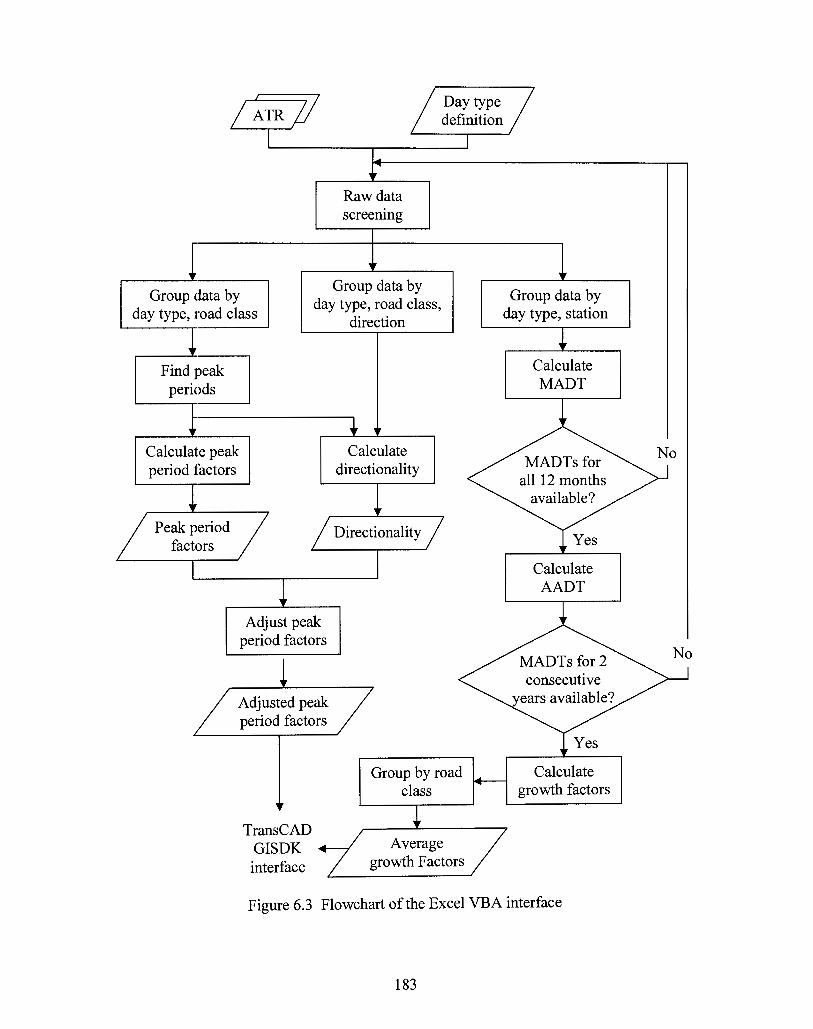
186

7. SUMMARY AND FINAL COMMENTS

7.1 Summary

Travel information systems can be divided into three groups – real-time, short-term

pre-trip and long-term pre-trip. The real-time information systems provide drivers

information during their trips, short-term pre-trip information systems shortly before

departure (normally within one day), and long-term pre-trip information systems one day

or more before departure. The real-time and short-term pre-trip information systems are

suitable for providing information about unexpected or nonrecurring events such as

incidents, while the long-term pre-trip information systems are designed to provide

information about expected events such as road construction. Previous research about

travel information systems has focused on analyzing and publicizing the effects of

unexpected events on traffic. Little attention has been given to long-term pre-trip

information systems because the real-time and short-term pre-trip information systems

can model both unexpected and expected events. However, because of the complicated

attributes of unexpected events, real-time and short-term pre-trip information systems

need further development to be effective in serving motorists. Long-term pre-trip

information systems can coexist with real-time and short-term pre-trip information

systems by meeting travelers’ needs at different times. Travelers with flexible schedules

may check with the long-term pre-trip information systems may schedule their trips that

187

require be set several days in advance and adjust trip plans at the time departure and

during driving according to the real-time and short-term-re-trip information systems for

the purpose of minimizing possible delays.

This study developed a long-term pre-trip information system called the Highway

Travel Information System (HTIS) by using an approach called Workzone Delay

Equilibrium Estimation (WDEE). WDEE attempts to find a new “steady state” for delay

based on the level of traffic that will use the workzone link after its existence has become

widely known. WDEE involves three steps – analysis for the “no information” scenario,

analysis for the “complete information” scenario and estimation of the delays during the

construction period. The WDEE process also allows the HTIS to estimate workzone

traffic flows (and therefore delays) for any time during the transition to the new steady

state.

A. Analysis for the “no information” scenario

The “no information” scenario simulates the condition at the beginning of a road

project when no drivers know that the new construction zone exists. Drivers will follow

the same routes they normally use during the same time frame, unaware of any newly

constrained capacities on some links on their routes. In the “no information” scenario,

the traffic flows on each link for a specific time frame at the beginning of road

construction are treated the same as when there was no construction. By applying proper

traffic volume forecasting techniques, the volumes on over 16,000 links in the Indiana

highway network can be estimated. Traditional traffic volume forecasting techniques are

not suitable for use in the HTIS because they require detailed data and long execution

time. A simplified traffic volume forecasting technique was developed for the purpose of

188

estimating flows on a large number of links. The main advantages of the simplified

traffic volume forecasting technique are that it can be applied to links without detailed

data and it can be applied to large network such as the Indiana statewide network.

B. Analysis for the “complete information” scenario

The “complete information” scenario simulates the case in which road construction

has been proceeding long enough that all drivers using that road know about it. Drivers

make informed decisions about whether to stay on the original route or divert to alternate

routes, based on their knowledge of the workzone and the surrounding network. Under

the assumption that drivers will only divert to alternate routes (rather than change their

departure time) to minimize delays, the travel demand between each O-D pair for a

specific time period will be the same for both the “complete information” and “no

information” scenarios. The demand for trips between each O-D pair for a specific time

frame can be estimated through the O-D estimation process using the “no information”

link volumes and the a priori matrix as inputs. This demand for trips between each O-D

pair is then assigned to a network having work zone capacity constraints to obtain the

link flows for the “complete information” scenario.

C. Estimation of the delays during the construction period

The actual traffic conditions during construction periods are in between the “no

information” and the “complete information” scenarios. The volumes at a workzone are

expected to decrease as construction proceeds and more drivers become aware of the

construction. The volumes stop decreasing as the system reaches an equilibrium state.

Because there are always a certain percentage of infrequent travelers that are not aware of

the construction, the volumes at the equilibrium state are higher than the “complete

189

information” link volumes. The relationship between the historical data and the age of

construction is hypothesized using a logistic function. This hypothetical relationship is

applied to the “no information” volumes and the volumes at the equilibrium state. The

link volumes at any time during the construction period can be, therefore, estimated.

The delays during the construction period are estimated using queueing analysis. The

service rate is the hourly workzone capacity based on the study of Dudek and Richards

(1981) and the arrival rate is the estimated link volumes obtained by applying the

hypothetical relationship to the two extreme link volumes (the “no information” and

“complete information” volumes). Knowing how the arrival rate is likely to change the

early stages of construction, the HTIS can estimate average delay per vehicle as more

drivers become aware of it.

The HTIS is divided into three subsystems – modeling, project scheduling, and web

access. The modeling and project scheduling subsystems are for management purposes

and the web access subsystem is for use by the traveling public. The modeling subsystem

is built with the Excel VBA and the TransCAD GISDK interfaces. The Excel VBA

interface implements the simplified traffic volume forecasting technique developed for

the HTIS. The TransCAD GISDK interface performs WDEE, which includes the

analysis of the “no information” scenario, the “complete information” scenario, the

estimation of link volumes during the transition construction period, delay estimation and

delay database generation. The project scheduling subsystem is also built on the

TransCAD GISDK interface. There are two major tasks for the project scheduling

subsystem. The first one is to manage project schedule databases. The second task is to

assist project scheduling personnel in determining proper scheduling strategies to avoid

190

excessive traffic delays by providing functions to adjust project starting date, end date,

and lane closure strategies in terms of workzone capacities. The web access subsystem is

built on several scripting languages, including Hyper Text Markup Language (HTML),

JavaScript, VB-script, and Active Server Pagers (ASP). The JavaScript and VB-script

provide an interactive environment. The ASP is a server-side-include scripting language,

which can generate personalized travel information upon receiving users’ requests.

Travelers may input the proposed departure time to retrieve information about expected

delays at workzones that are active at the departure time and use the information to plan

their trips up to two months in advance.

The HTIS requires routine maintenance in order to provide updated travel

information. Most of the maintenance tasks are accomplished during routine use of the

subsystems.

7.2 Final Comments

The HTIS can be further refined to improve the accuracy of workzone delay estimates

and to enhance the function of assisting project scheduling in the following five ways.

(1) New techniques in traffic volume forecasting, traffic assignment, O-D estimation, and

workzone delay estimation may be applied in the HTIS. Because the architecture of

the HTIS is highly modularized, each part of the analysis in the modeling subsystem

of the HTIS is independent from others. New techniques for any of the parts can be

plugged into the HTIS easily without changing an other part of the HTIS. However,

the application of new analysis techniques needs to consider the availability of

required data and the feasibility of applying it on a large network.

191

(2) The accuracy of workzone delay estimates can be further verified. Only two surveys

were conducted to validate workzone delay estimates (both on I65 between SR43 and

SR18). The results were satisfactory, but the accuracy of the delay information

generated by the HTIS would benefit from further verification.

(3) The effects of information available via the World Wide Web (WWW) on travelers’

behavior require further study. Currently the WWW has not been used to disseminate

information about workzone delays. Travelers make decisions based on the

information provided via traditional media such as TV, radio and variable message

signs (VMS). The information provided by the HTIS via the WWW may affect

travelers’ behavior to different degrees. By understanding the aggregate effects of the

WWW on the traffic, the HTIS may provide more accurate delay estimates.

(4) The function of assisting project scheduling can be further extended. The information

provided in the HTIS for assisting project scheduling is the total delay based on

current scheduling strategy. A sensitivity analysis of project starting dates, end dates

and lane closure strategies on system performance may be added.

(5) Observed data about hourly volumes during the construction period can be used to

analyze the relationship between hourly workzone approach volumes and the age of

construction. The plan was to take advantage of the continuous data provided by the

Automated Traffic Recorder (ATR) stations by finding construction sites located

downstream of the ATR sites. However, no suitable data for such cases have been

obtained so far. In the rare cases in which an ATR site was immediately upstream

from a workzone, equipment malfunctions prevented a detailed analysis of traffic

volume trends. An approximate relationship between hourly volumes and the age of

192

construction has been hypothesized. The relationship between hourly volumes and

the age of construction based on observed data may depict the aggregate effects of

travelers’ behavior during the construction period more accurately.

193

LIST OF REFERENCES

Abraham B. and Ledolter J. (1983) Statistical methods for forecasting. John Wiley & Son Ltd., New York. Adler J. and Blue V. (1998) Toward the design of intelligent traveler information systems. Transportation Research Part C 6, pp.157-172. Allen, Ziedman, Rosenthal, Stein, Torres and Halati (1991) Laboratory assessment of driver route diversion in response to in-vehicle navigation and motorist information systems. Transportation Research Record 1306, pp.82-91. Arnott R., de Palma A. Lindsey R. (1991) Does providing information to drivers reduce traffic congestion? Transportation Research Part A, Vol. 25A, No. 5, pp.309-318. Barfield W., Haselkorn M., Spyridakis J. and Conquest L. (1991) Integrating commuter information needs in the design of a motorist information system. Transportation Research Part A, Vol. 25A, Nos. 2/3, pp.71-78. BGC (1993) FMC documentation, v. 2.10, Bureau Goudappel Coffeng bv, Deventer, The Netherlands. Boruff D. (1994) An investigation into the effects of highway construction on driver behavior. Indiana Department of Transportation. Indianapolis, IN. Caliper Inc. (1999) Travel Demand Modeling with TransCAD 3.5. Newton, MA. Cambridge Systematics, Inc. (1998) Major Corridor Investment-Benefit Analysis System: Model Documentation Part I: Indiana Statewide Travel Model. Cassidy M. and Han L. (1993) Proposed model for predicting motorist delays at two-lane highway work zones. Journal of Transportation Engineering, Vol. 119, No. 1, pp27-42. Dixon K., Hummer J. and Rouphail N. (1998) Comparison of rural freeway work zone queue length estimation techniques: a case study. Transportation Research Board, 77th Annual Meeting. Washington, D.C.

194

Dougherty M. and Cobbett M. (1997) Short-term inter-urban traffic forecasts using neural networks. International Journal of Forecasting, Vol. 13, No. 1, pp.21-31. Dudek C. and Richards S. (1981) Traffic capacity through work zones on urban freeways. Texas Transportation Institute. Research Report 228-6. College Station, Texas. Dudek C., Richards S. and Buffington J. (1986) Transportation Research Record 1086, pp.20-30. FHWA (1995) Traffic Monitoring Guide. FHWA-PL-95-031. Federal Highway Administration. Hamerslag R. and Immers B. (1988) Estimation of trip matrices: shortcomings and possibilities for improvement. Transportation Research Record 1203, pp.27-39. HCM (1997) Highway Capacity Manual, Special Report 209, 3rd edition. Transportation Research Board. Chapters 1 and 3. Jha M. and Sinha K. (1996) Effective scheduling of road and bridge closures: phase II. Joint Highway Research Project. FHWA/IN/JHRP-96/7. Purdue University. Jiang Y. (1999) Traffic characteristics and estimation of traffic delays and user costs at Indiana freeway work zones. Indiana Department of Transportation, Division of Research. FHWA/INDOT/SPR-2121. West Lafayette, IN. Khattak A., Schofer J. and Koppelman F. (1995) Effect of traffic information on commuters’ propensity to change route and departure time. Journal of Advanced Transportation, Vol. 29, No. 2, pp.193-212. Khattak A., Yim Y. and Stalker L. (1999) Does travel information influence commuter and noncommuter behavior? Transportation Research Record 1694, pp.48-58. Kirby H., Watson S. and Dougherty M. (1997) Should we use neural networks or statistical models for short-term motorway traffic forecasting? International Journal of Forecasting, Vol. 13, No. 1, pp.43-50. Lam W. and Lo H. (1990) Accuracy of O-D estimation from traffic counts, Traffic Engineering Control, Vol. 30, No. 6, pp.358-367. Memmott J. and Dudek C. (1982) A model to calculate the road costs at work zones. Texas Transportation Institute. Research Report 292-1. College Station, Texas. Ortuzar J. and Willumsen L. (1996) Modelling Transport, 2nd Edition. John Wiley & Son Ltd., New York. Section 10.2 ~10.5, 10.7 and 12.4.

195

Pavlis Y. and Papageorgiou M. (1999) Simple decentralized feedback strategies for route guidance in traffic networks. Transportation Science, Vol. 30, No. 3, pp.264-278. Polydoropoulou A., Ben-Akiva M. and Kaysi I. (1994) Influence of traffic information on driver’ route choice behavior. Transportation Research Record 1453, pp.56-65. Nemeth Z. and Rouphail N. (1982) Lane closures at freeway work zones: simulations study. Transportation Research Record 869, pp.19-25. Nielsen O. (1993) A new method for estimating trip matrices from traffic counts. Paper 1993-3, Institute of Roads, Traffic and Town Planning, the Technical University of Denmark. Robertson D., Palumbo N. and Rice R. (1995) Impact of expressway reconstruction on adjacent traffic operations. ITE Journal, Vol. 65, No. 8, pp.43-53. Scheaffer R. and McClave J. (1990) Probability and statistics for engineers, 3rd Edition. PWS-KENT Publishing Company. pp.585-592, 668. Sefton D. (2000) Daily web surfing now the norm. Retrieved August 24, 2000 from the World Wide Web: http://www.usatoday.com/life/cyber/tech/cth591.htm Smith B. and Demetsky M (1997) Traffic flow forecasting: comparison of modeling approaches. Journal of Transportation Engineering, Vol. 123, No. 4, pp.261-266. Soares R. and Najafi F. (1998) User costs at the work zone. Transportation Research Board, 77th Annual Meeting. Washington, D.C. Thatcher A, Kannisto V, and Vaupel J (1998) The Force of Mortality at Ages 80 to 120. Odense University Press, Denmark. Chapter 2. The CQ Researcher (1999) Congestion Is Increasing. The amount of severe congestion more than double from 1982 to 1996. The CQ Researcher, Vol. 9 No. 32, pp.735-744. Yun S., Namkoong S., Rho J., Shin S. and Choi J. (1998) A performance evaluation of neural network models in traffic volume forecasting. Mathematical and Computer Modelling, Vol. 27, No. 9-11, pp.293-310. Voort M., Dougherty M. and Watson S. (1996) Combining Kohonen maps with ARIMA time series models to forecast traffic flow. Transportation Research Part C, Vol. 4, No. 5, pp.307-318. Wang K. and Elliott R. (1995) Design considerations for distributed, multimedia-based highway information system. Transportation Research Record 1505, pp.95-102.

196

Whitford R. and Opsuth J. (1996) Congestion estimates for Indiana state highway system. Joint Highway Research Project. FHWA/IN/JHRP-96/8. Purdue University. Yang J. and Fricker J. (1996) Estimating statewide trip tables from vehicle classification counts. Joint Highway Research Project. FHWA/IN/JHRP-95/15. Purdue University. Zhang J., Leiman L and May A. (1989) Evaluation of operational effects of freeway reconstruction activities. Transportation Research Record 1232, pp.27-39.

197

APPENDIX HIGHWAY TRAVEL INFORMATION SYSTEM USER’S GUIDE

The application of the Highway Travel Information System (HTIS) is explained in

three parts: the Excel VBA interface, the TransCAD GISDK interface, and the web

access interface. The Excel VBA interface is for use by the modeling personnel. The

TransCAD GISDK interface is for use by both the modeling and project scheduling

personnel, and the web access interface is for use of public users (travelers). The

relationship of these three users’ interfaces is shown in Figure A.1. Through the Excel

VBA interface, the peak period factors are generated and passed to the TransCAD

GISDK interface. The delay database is then generated by the TransCAD GISDK

interface and passed to the web access interface. Finally, public users may access the

delay database through the web access interface.

Refer to Section 6.1 for development considerations of the Excel VBA interface and

the modeling task in the TransCAD GISDK interface, to Section 6.2 for development

considerations of the project scheduling task in the TransCAD GISDK interface, and to

Section 6.3 for development considerations of web access interface.

198

A.1 Excel VBA Interface

The Excel VBA interface has for two purposes: (1) To generate peak period factors,

which will be stored in a dBase IV file. (2) To calculate monthly average daily traffic

(MADT) for each ATR station. The framework of the Excel VBA interface is shown in

Figure A.2.

Step 1: Enter the Excel VBA interface

Enter the Excel VBA interface by double clicking on the icon “atrmacro.xls.” A

message warning that the file contains macros will appear. Enable the macros, so that

this program works properly. After this program has been entered, the introduction

menu that briefly explains the functions of this program will appear on the screen

(Figure A.3). By pressing the “Start” button, users can see the main menu for this

program (Figure A.4).

Step 2: Inputs for the Excel VBA interface

The “Option” in the main menu allows the user to specify which function to

execute: “generate peak period factors” or “calculate MADT.” The “generate peak

period factors” function calculates peak period factors based on a file of Automated

Traffic Recorder (ATR) historical data. The “calculate MADT” function obtains the

monthly average daily traffic (MADT) for each ATR station. The inputs for these two

functions are listed as follows:

(1) Inputs for the “generate peak period factors” function

• An ATR file, whose file name will be shown as the “Current ATR file”;

• Additional inputs for generating peak period factors. (See Figure A.4.)

(2) Input for the “calculate MADT function”

199

• A set of ATR files for up to 12 files: The file name of the ATR file that is being

processed will be shown as the “Current ATR file.”

Each input is explained below.

(1) Current ATR file:

The “Current ATR file” shows the ATR file that is being processed. By clicking

the “Open ATR file(s)”, a dialog box will appear (Figure A.5). This program can

handle two file types: the raw data in federal format (*.fed) and in Excel format

(*.xls). The ATR files in federal format are obtained from the INDOT’s Roadway

Management Division. These files contain a lot of rows of continuous text, whose

entries are distinguished by column numbers (Figure A.6). Each row of data

represents hourly volumes in a specific direction for a specific ATR station during a

specific hour on a specific day.

If the ATR files in federal format are chosen, this program will transfer the files

into the Excel format and save using the same name. For example, if the file

“maytr98.fed” is chosen, it is transferred and saved as “maytr98.xls.”

Users may select one ATR file if the option “Generate peak period factors” is

chosen. If the option “Calculate MADT” is chosen, users may select up to 12 ATR

files to process by pressing the “Control” key on the keyboard and selecting multiple

files from the list of file names. When multiple files are chosen to be processed, the

year and month of the ATR data in the file that is currently being processed are

shown in the two textboxes next to the “Open ATR file(s)” button (Figure A.4).

200

(2) Additional inputs for generating peak period factors:

This group of inputs is only required if the option is to generate peak period

factors. If the option “Calculate MADT” is selected, this group of inputs is disabled.

The inputs in this group include “Year of Departure”, “Base Year of ADT”, “Month

of Departure”, “Enter Special Days” and “Annual Growth Factors.” They are

discussed below.

• Year of Departure

The “Year of Departure” is for the calculation of the total growth factors, which

are used to update the ADTs in the network database to the year of a trip’s

departure. An example input is like “2000.”

• Base Year of ADT

The “Base Year of ADT” is also for the calculation of the total growth factors of

ADTs. Currently the ADTs in the network database are for the year 1995, the

default value of the “Base Year of ADT.” If the ADTs in the network database are

updated, the default value of the “Base Year of ADT” should be updated

accordingly.

• Month of Departure

The “Month of Departure” can not be changed by the user. The “Month of

Departure” is automatically set to be the same as the month of the ATR data, based

on the assumption that each month has its unique traffic patterns. For example, the

ATR file for May 1998 can only represent the traffic patterns for May.

201

• Enter Special Days

The “Enter Special Days” button allows the user to define day types in addition

to the two default day types, weekdays and weekends. The special days are referred

to as holidays and days with special events whose traffic conditions are different

from normal weekdays and weekends. For example, special days can be

Thanksgiving and days affected by the Indianapolis 500 car race. When clicking

the “Enter Special Days” button, the special days input menu will appear (Figure

A.7). Users can choose to specify special days by date or by day of week. Two

examples of specifying special days are shown in Figure A.7. The first special day

is specified by date, May 13. The second special day is specified by day of week,

the third Sunday in May. This program allows entry of up to 10 different special

days.

• Annual Growth Factors

The “Annual Growth Factors” input is required to calculate the total growth

factor between the year of departure and the base year of ADT. The default values

are the annual growth factors between 1998 and 1999 that are the latest available

from the Roadway Management Division of INDOT (Table 5.9) as this project is

completed. Users may edit these values if desired.

Step 3: Execute the Excel VBA interface

By clicking the “Execute” button in Figure A.4, this program will execute the

function selected in the “Options” input. The two options available are “generate peak

period factors” and “Calculate MADT.” Each function is explained as follows.

202

(1) Generate peak period factors

The program will first define the peak periods for different road classes and day

types based on the current ATR file. A pop-up window will show the definitions of

peak periods based on the current ATR file, providing users a chance to modify the

definitions (Figure A.8). The final results of estimated peak period factors are stored

in a database named “peakfac.dbf.” An example output file of peak period factors is

shown in Figure A.9. The total growth factors are shown only in the first four rows

of Figure A.9, because their values depend only on road class and not on day type.

The ROADCLASS values of 0 through 3 in Figure A.9 represent “rural interstate

highway”, “rural other highway”, “urban interstate highway” and “urban other

highway.” The DAYTYPE values of 0 through 2 represent “weekday”, “weekend”

and the special day specified by the user. The special day in Figure A.9 is the second

Sunday in May. AMPEAK, PMPEAK and OFFPEAK represent the peak period

factors for AM-peak, PM-peak and off-peak periods. These values are the adjusted

peak period factors, which combine peak period factors and directionality.

AMBEGIN, AMEND, PMBEGIN and PMEND represent the beginning and end of

AM-peak and PM-peak periods. TGROWTH represents the total growth factors,

which are the growth factors from the base year of ADTs to the year of departure.

REMARK provides definitions of the day types.

(2) Calculate MADT

The program will process one ATR file at a time and calculate the MADT for

each ATR station. The resulting MADTs are stored in a file with the name of the

ATR file and “ADT” appended to it. For example, the results of MADTs for the

203

ATR file “maytr98.xls” are stored in a file named “maytr98ADT.xls.” An example

output file is shown in Figure A.10. The “Station” represents the ATR station ID.

“RoadClass” and “DayType” have the same definitions as in the file of peak period

factors (Figure A.9). MADT represents the monthly average daily traffic at the

station for the specific road class and day type.

A.2 TransCAD GISDK Interface

The framework of the TransCAD GISDK interface is shown in Figure A.11. There

are two groups who need to use the TransCAD GISDK interface: the modeling group and

the project scheduling group. By entering the TransCAD, a pop-up window will show

for choosing an application (Figure A.12). By selecting the “HTIS” application, the

TransCAD GISDK interface will show the main menu (Figure A.13), which allows the

user to select the proper user group. The user will be guided to the “modeling menu” and

the user of the project scheduling group to the “project scheduling” menu. The functions

provided in the modeling and project scheduling subsystems are listed as follows.

(1) The functions for the modeling subsystem provided in the TransCAD GISDK

interface in the modeling subsystem include:

• Link volume forecasting;

• Delay verification;

• Delay database generation and conversion.

(2) The functions provided for the project scheduling subsystem include:

• Maintaining schedule database;

• Evaluating current scheduling strategy.

204

A.2.1 Modeling subsystem

The three functions provided in the modeling subsystem – link volume forecasting,

delay verification and delay database generation – are sequential processes. The link

volume forecasting needs to be processed first, the delay verification second, and the

delay database generation last.

A.2.1.1 Link volume forecasting

The modeling input menu (Figure A.14) will appear if the option “Modeling” is

chosen in the main menu.

Step 1: Inputs for link volume forecasting

Users may provide different combinations of input files to perform two different

sets of link volume forecasting analyses:

(1) Inputs for the “no information” link volume forecasting

• A map file in TransCAD map format (*.map) (Figure A.15);

• A peak factor file in dBaseIV format (*.dbf) (Figure A.9);

• A construction schedule file in dBaseIV format (*.dbf) (see Step 2 in Section

A.2.2);

• An existing hourly volume file in dBaseIV format (*.dbf) (Figure A.16) or a file

name for storing hourly volumes.

(2) Inputs for both the “no information” and the “complete information” link volume

forecasting

• A map file in TransCAD map format (*.map);

• A peak factor file in dBaseIV format (*.dbf);

205

• A construction schedule file in dBaseIV format (*.dbf);

• An existing hourly volume file in dBaseIV format (*.dbf) or a file name for

storing hourly volumes.

• An O-D matrix file in TransCAD matrix format (*.mtx) (Figure A.17).

Step 2: Execute the link volume forecasting

The forecasting process will be executed automatically after the input files are

given. No manual operations are required. Users should be aware that the whole

process of the “complete information” volume forecasting can take a long time

depending on the number of day types and the number of combinations of different

construction projects active at the same time. The execution time for a single day type

and a set of construction projects active at the same time is about 40 to 50 minutes. If

only a preliminary estimate of traffic conditions is needed, the “no information” link

volume forecast can provide some useful trends. However, if users need to build a

delay database, the “complete information” link volume forecasting is required.

Step 3: Outputs from link volume forecasting

(1) Outputs from “no information” volume forecasting

The outputs from “no information” volume forecasting are the “no information”

link volumes, which are stored in the file of hourly volumes. The fields stored in the

file are named as the combination of day type abbreviation, a serial number for

special day types, period abbreviation and “VOL”. The day type abbreviations for

weekdays, weekends and special days are “WD”, “WE” and “SP.” The day type of

special days is distinguished by a serial number starting from 1 to the maximum

allowable special day types of 10. The period abbreviations for AM-peak, PM-peak

206

and off-peak periods are “AM”, “PM” and “OFF.” For example, the field name of

the “no information” hourly volume during AM-peak period for a typical weekday is

“WDAMVOL”, and the field name of the “no information” hourly volumes during

off-peak period for the first special day is “SP1OFFVOL.”

(2) Outputs from “complete information” volume forecasting

The outputs from “complete information” volume forecasting are the “complete

information” link volumes. “Complete information” volume forecasting involves a

combination of transportation planning analyses, such as O-D estimation and traffic

assignment. The number of applications of O-D estimation and traffic assignment

that need to be repeated are explained in Section 6.1. Both the O-D estimation and

the traffic assignment processes will generate intermediate outputs before the final

outputs – the “complete information” link volumes – are generated. The intermediate

outputs for O-D estimation and traffic assignment, and the final outputs for the

“complete information” volume forecasting, are explained as follows.

• Intermediate outputs for O-D estimation

Several intermediate files will be generated from each application of O-D

estimation and traffic assignment when “complete information” link volume

forecasting is performed. Each application of O-D estimation will generate two

intermediate outputs.

(a) An estimated O-D table in TransCAD matrix format (*.mtx) for use by the

traffic assignment process, and

(b) A binary file (*.bin) of estimated link volumes for comparison with the

“observed link volumes” and for use as one of the inputs for O-D estimation.

207

The “observed link volumes” are those found in the “no information” link

volume forecast based on the assumption that the demand of each O-D pair

before construction and during construction are the same. (See Section 5.3 for

detailed explanations.)

To distinguish the outputs of each application of O-D estimation, both the

estimated O-D table and estimated link volumes are named as the combination of

“OD”, day type abbreviation and period abbreviation. The day type abbreviations

for weekdays and special days are “WD”, and “SP1” through “SP10.” The period

abbreviations for AM-peak, PM-peak and off-peak periods are “AM”, “PM”, and

“OFF.” For example, when generating the O-D table for the “no information” link

volumes during AM-peak period in a typical weekday, the day type code for

weekdays is “WD” and the period abbreviation is “AM.” The estimated O-D table

is named “ODWDAM.mtx” and the binary file of the estimated link volumes is

named “ODWDAM.bin.”

• Intermediate outputs for traffic assignment

Each application of traffic assignment will generate an intermediate binary file

(*.bin) of the “complete information” hourly volumes for all links. The binary file

of the “complete information” hourly volumes is named in a different way from the

output files for O-D estimation, because of the limitation of TransCAD in dealing

with long file names (maximum of 8 characters). The name of the binary file of the

“complete information” hourly volumes is as the combination of “TA”, day type

code, period code and construction starting or ending date. The day type codes are

0 for weekdays, and 2 through 12 for special days . The period codes for AM-peak,

208

PM-peak and off-peak periods are 0, 1 and 2. The construction starting or ending

date is the combination of month and date. For the example, the binary file of the

“complete information” hourly volumes during AM-peak period (0) for a typical

weekday (0) between May 2 (0502) and the next time when there is a construction

project starting or ending is named “TA000502.bin.”

• Final outputs for “complete information” volume forecasting

The final outputs, the “complete information” hourly volumes from traffic

assignment, will be copied to the file of hourly volumes with the field names similar

to the ones with the “no information” link volumes, using the combination of “LB”,

day type abbreviation, period abbreviation, “VOL”, and time span code. The “LB”

represents the lower bound of workzone link volumes, which are the “complete

information” link volumes. The definitions for day type abbreviation, period

abbreviation and “VOL” are the same as the definitions for the “no information”

link volumes. The time span code is a serial number to distinguish different time

spans, each of which represents the time span between when a project starts or ends

and the next time a project starts or ends, or a special day occurs (Figure 6.5). The

first time span is always for the period between the first day of the specific month

and the first time a project starts or ends in the month. The following time spans

are defined as between the time when a project starts or ends and the next time a

project starts or ends. The final time span is between the last time when a project

starts or ends before the end of the month and the end of the month. For example,

there is a special day in the first time span of a specific month, which is between the

first day of the month and the time the first project starts or ends. The field name of

209

the “complete information” hourly volumes during AM-peak period for a typical

weekday in the first time span is “LBWDAMVOL1”, and the field name of the

hourly volumes during the off-peak period for the special day in the first time span

is “LBSP1OFFVOL1.”

A.2.1.2 Delay verifications

The main menu for verifying possible delays according to the forecasted volumes will

appear after the volume forecasting process (Figure A.18).

Step 1: Inputs for delay verification

The inputs required are the day type, time of day and a selected link for evaluation.

They are addressed as follows.

(1) Day type

The day type options are read from the peak period factor file that is given in the

modeling input menu (Figure A.18). The day type, together with the time of day in

the following input items, determine which field of hourly volumes in the file of

hourly volumes to retrieve for verifying delays.

(2) Departure time

The “Departure time” is to specify a departure time for delay estimation. The

“Departure time” is in one-hour increments. The delays during the one-hour period

are estimated based on the corresponding forecasted hourly volumes.

210

(3) A selected link

The link for evaluation is selected by clicking on the “Select a link” button on

the menu first. The pointer of the mouse will become a cross when the mouse is

moved on the map. The user may select a link by clicking on it.

Step 2: Execution and the outputs for delay verification

When a link on the map is selected, the color of the link is changed to red and a

pop-out message box with information of estimated delay is shown. The upper bound

delay is shown if only the “no information” link volumes are forecasted (Figure

A.19). The adjusted delay is shown if both the “complete information” and the “no

information” link volumes are available (Figure A.20). Users can continue the delay

evaluation without having to click on the “Select a link” button again if the pointer of

the mouse remains a cross while moving the mouse over the map. When the link

delays are not acceptable, users may either adjust the peak period factors in the peak

factor file (Figure A.9) or regenerate the peak factor file by changing the “Annual

Growth Factors” in Figure A.4 or the definitions of peak periods in Figure A.8.

A.2.1.3 Delay database generation and conversion

Step 1: Delay database generation

If both the “no information” link volumes and the “no information” link volumes

are available and the accuracy of the estimated delays is verified by the user, the delay

database can be generated by clicking on the “Generate delay database” button on the

main menu (Figure A.18). The file of the delay database can be saved in dBaseIV

format (*.dbf). The name of the file can be input in the pop-out dialog box (Figure

211

A.21). After the delay database is generated, the tasks in the TransCAD GISDK

interface are finished.

Step 2: Delay database conversion

The delay database needs to be converted into Microsoft Access format before the

public can access it. The file conversion process under Microsoft Access 2000 begins

by creating a new empty database. Select the option “Blank Access database” under

the group “Create a new database using” (Figure A.22) or by selecting “File” and then

“New” from the menu bar. By selecting “File”, “Get External Data” and then “Import”

from the menu bar, a pop-up dialog box will appear, asking which file to import (Figure

A.23). Users need to change the “Files of type” to “dBaseIV (*.dbf) and then select the

file name of the delay database from the file lists. After importing the data, the delay

database in Microsoft Access format can be uploaded to the web server for public

access. An example delay database in Microsoft Access format is shown in Figure

A.24.

A.2.2 Project scheduling menu

The functions provided for project scheduling personnel are to maintain the project

schedule database and to evaluate current scheduling strategy. Maintaining the schedule

database involves adding, updating and/or deleting construction projects including the

start date, end date, number of lane closures and a brief description of the project content.

Evaluating current scheduling strategy uses two performance indices: “Link delay” and

“Total delay.” “Link delay” is used to check a specific link that is under construction,

while “Total delay” is for checking the system performance for the current scheduling

212

strategy. Because the purpose of evaluating current scheduling strategy is to calculate

performance indices based on a schedule database, this function is embedded in schedule

management. (See Figure A.11.)

Step 1: Inputs to the project scheduling subsystem

If the option “Project Scheduling” is chosen in the “User Group” of the HTIS main

menu (Figure A.12), the project scheduling management input menu (Figure A.25) will

appear. Users may provide different combinations of input files to perform two

different combinations of functions.

(1) The inputs required for scheduling management include:

• A network file in TransCAD map format (*.map);

• Either an existing construction schedule file in dBaseIV format (*.dbf) or a file

name for storing construction schedules.

(2) The inputs needed for evaluating current scheduling strategy depend on the purpose

for evaluation. If the purpose is to get a rough idea of the impacts on traffic, only the

“no information” analysis, which produces the upper bound of link delays, is needed.

If the evaluation is for considering the effects of construction during transition period

when the workzone is not known to most of the travelers, both the “no information”

and the “complete information” analyses are required.

• Inputs for the “no information” analysis

- A map file in TransCAD map format (*.map) (see Figure A.15);

- A peak factor file in dBaseIV format (*.dbf) (see Step 3 in Section A.1 and

Figure A.9);

213

- An existing construction schedule file in dBaseIV format (*.dbf) (see Step 2 in

this section);

- An existing hourly volume file in dBaseIV format (*.dbf) (see Step 3 in Section

A.2.1.1 and Figure A.16).

• Inputs for both the “no information” and the “complete information” analyses

- A map file in TransCAD map format (*.map);

- A peak factor file in dBaseIV format (*.dbf);

- A construction schedule file in dBaseIV format (*.dbf);

- An existing hourly volume file in dBaseIV format (*.dbf) or a file name for

storing hourly volumes.

- An O-D matrix file in TransCAD matrix format (*.mtx) (Figure A.17).

Step 2: Schedule management

The main menu for project scheduling management will appear after the required

inputs are provided (Figure A.26). This menu is a simple database management system

with the function of connecting the database to the geographic attributes. Each record

in the scheduling database contains fields for the project beginning date, end date,

workzone capacity, a brief description of the project, link ID as noted in TransCAD,

and the coordinates of two end nodes for the link. The link ID and node coordinates are

automatically linked to the inputs above.

(1) “Add”, “Save edited”, and “Delete” functions

Users must select a link by clicking on the “Select a link” button on the menu

before adding, editing and deleting any records. The function of “Select a link” here

is the same as it was in the delay verification menu in the modeling subsystem. Once

214

the button is clicked, the pointer of the mouse will change into a cross when the

mouse is moved over the map. Users may select a link on which to apply

construction constraints, by clicking on the button “Add”, “Save edited” or “Delete”

to add, edit or delete a record in the construction schedule database. These three

buttons are disabled if no link is selected, because no geographic attributes can be

linked to the manual inputs. Each time a record is added, edited or deleted, the

modifications are directly saved in the database. Therefore, there is no need to save

the database.

(2) “Clear” function

The function of “Clear” in Figure A.26 is to empty the current manual inputs to

allow more convenient entry of a different set of inputs.

(3) “Show all” function

The function of “Show all” is to show the existing records in the scheduling

database. When there are records in the scheduling database, both the records and the

locations will be displayed in a table and on the map when the “Show all” button is

clicked. The records in a table are shown in a new window and the locations on the

map are shown in thick dark green lines (Figure A.27). This function is disabled

when there is no record in the scheduling database.

Step 3: Evaluation of current scheduling strategy

The function of evaluating current scheduling strategy provides two performance

indices: “Link delay” and “Evaluate schedule.” These two functions are embedded in

the schedule management menu (Figure A.26).

215

(1) “Link delay” function

The function of “Link delay” is to display the estimated delay on any selected

link, given to the current scheduling strategy. When this function is chosen, the

project scheduling subsystem is linked to the “no information” and the “complete

information” link volume forecasting in the modeling subsystem. After finishing the

“no information” and the “complete information” link volume forecasting, the users

in the project scheduling group will be led to the delay verification menu in the

modeling subsystem (Figure A.18). It should be noted that this function may require

a long execution time depending on the number of day types and the number of

combinations of different construction projects active at the same time. The

execution time for a single day type and a set of construction project active at the

same time is about 40 to 50 minutes. The user should use this function only if all

schedules have been updated. If not all of the inputs for evaluating current

scheduling strategy are provided in the input menu for the project scheduling

subsystem (Figure A.25), this function is disabled.

(2) “Evaluate schedule” function

Using the function “Evaluate schedule”, the total delay on all workzone links for

selected periods is calculated. The user is led to the scheduling evaluation menu

(Figure A.28). This function may also take a long time to execute. As with the

execution time for the function “Link delay”, the total execution time depends on the

number of day types and the number of combinations of different construction

projects active at the same time. The execution time for a single day type and a set of

construction project active at the same time is about 40 to 50 minutes. The user

216

should use it only if all schedules have been updated. If not all of the inputs for

evaluating current scheduling strategy are provided in the input menu for the project

scheduling subsystem (Figure A.25), this function is disabled.

The “Evaluate schedule” function is completed with the following two processes.

• Determine evaluation period

Users may determine the evaluation period for total delay in two ways.

- Click the “Select a link” button in Figure A.28 and then click on a desired link

that belongs to a construction project. The total system delay during the time

when the specific construction project is in progress within the month specified

in the peak factor file will be calculated.

- By entering the start date and the end date as evaluation period: The total delay

during the evaluation period will be calculated.

• Calculate expected delay for all links

After defining the evaluation period, users are led to the modeling subsystem to

calculate the expected delays of all links under construction during the specified

evaluation period. The sum of the product of the expected delays and volumes for

each workzone link is defined as the total statewide delay for the specific period of

time. The total delay for the specific period of time is then passed back to the

project scheduling subsystem and shown in a message box (Figure A.29).

The calculation of total delay may be done again in two ways.

- Change the evaluation period in the scheduling evaluation menu (Figure A.28)

and calculate the total delay based on the existing scheduling strategy;

217

- Press the “Back” button to the schedule management menu (Figure A.26),

change scheduling strategy, and then press the “Evaluate schedule” button to

return to the schedule evaluation menu for calculating total delay based on the

updated scheduling strategy. Schedule strategies can be changed by inputting

different project beginning dates, project end dates, or number of lanes closed

that is reflected by entering different workzone capacities. The scheduling

evaluation can be repeated until the project schedules have been improved as

much as possible, according to the judgment of the project scheduler.

A.3 Web Access Interface

The framework of the web access interface is shown in Figure A.30. The web access

subsystem is an interactive interface for highway travelers to get information about

delays at workzones via web browsers. Travelers may repeatedly query the subsystem by

changing the departure time.

Step 1: Enter web access interface

Currently, the web access subsystem is uploaded to a temporary web server that

supports ASP scripting. The temporary web address for the web access subsystem is

http://domaindlx.com/shuling/test/htis.htm. The official web address for the subsystem

will be determined by INDOT.

Step 2: Inputs for the web access interface

The homepage of the web access subsystem is shown in Figure A.31. Travelers

may follow the instructions on the page to obtain delay information for a specified time.

Two inputs are required for the web access subsystem:

218

(1) Departure date

The departure date can be any date between current date and the end of the next

month. More information can be provided if the construction schedules can be set

more than one month in advance. See Section 6.3 for more explanations.

(2) Departure time

The departure time is in hourly periods. If a traveler plans to departure at

7:30AM, the departure time of 7:00AM ~ 8:00AM should be selected.

Step 3: Outputs for the web access interface

After the two required inputs are given, travelers may click on the “Submit” button

to view estimated delays due to workzones at the specific time. Figure A.32 shows the

response page of the query results. Because the delay database has not been

established, the ATR station database is used for illustration purpose. The search

criteria for the ATR station database is “County ID” in contrast to the search criteria

“Departure Date” and “Departure Hour” for the delay database. Each icon in Figure

A.32 is supposed to represent a construction project workzone expected to be in place

during the time specified by travelers.

The web access subsystem provides two ways to view delay information for each

project:

(1) By moving the mouse on top of a workzone icon

A “tip box” will appear, showing the estimated delay for that workzone. For

example, the tip box in Figure A.32 shows “Site 2 on US 52: Delay = 46 minutes”

when the mouse is moved on top of the workzone Site 2.

219

(2) By clicking on the workzone icon

The detailed information about the corresponding project will appear in the

textbox to the right of the map. For example, the detailed information in Figure A.32

shows “Site 2 on US 52: Delay = 46 minutes. This project will be finished by 9

December 2000.” when the icon of the workzone Site 2 is clicked. Each time an icon

is clicked, the contents of the textbox is automatically changed.

Travelers may input a different departure date and time right under “New search” in

the same page without having to go back to the homepage (Figure A.32). Because the

processing time for each query is only a few seconds, travelers can query many times in

a few minutes and decide on the best departure time for their trips.

220

Figure A.1 Relationship of HTIS users’ interfaces

Excel VBA interface

Peak period factors

TransCAD GISDK interface

Delay database

Web access interface

Possible delays on links under construction

Modeling Subsystem

Project Scheduling Subsystem

Web Access Subsystem

221

Figure A.2 Framework of the Excel VBA interface

Execute

HTIS Excel VBA

introduction menu

Exit Open

ATR files Enter special

days

Special days input menu

Start

HTIS Excel VBA main menu

Peak period factors


222

Figure A.3 Excel VBA introduction menu for the modeling subsystem

223

Figure A.4 Excel VBA main menu for modeling subsystem

224

Figure A.5 Open ATR files from the Excel VBA main menu

225

Figure A.6 An example ATR file in federal format (*.fed)

226

Figure A.7 Special days input menu in the Excel VBA interface

227

Figure A.8 Definitions of peak periods for different day types and road classes

228

Figure A.9 The output file of the peak period factors from the Excel VBA interface

229

Figure A.10 The output file of MADTs from the Excel VBA interface

230

Figure A.11 Framework of the TransCAD GISDK interface

Execute Exit

Select a link Back

Execute Exit

Link delay Select a link

Add Save Delete

Back Evaluate schedule

Execute Back

HTIS TransCAD main menu

Modeling subsystem input menu

Project scheduling subsystem input menu

Delay verification

menu

Schedule management

menu

Schedule evaluation

menu

Delay database

generation

Delay database

Excel VBA interface

Web access interface

231

Figure A.12 Screen capture for entering the TransCAD GISDK interface for HTIS

232

Figure A.13 Main menu of the TransCAD GISDK interface

233

Figure A.14 Input menu for TransCAD GISDK interface in modeling subsystem

234

Figure A.15 A map file in TrnsCAD map format (*.map)

235

Figure A.16 An existing hourly volume file in dBase IV format (*.dbf)

236

Figure A.17 An O-D matrix file in TransCAD matrix format (*.mtx)

237

Figure A.18 Main menu for delay verification for TransCAD GISDK interface in

modeling subsystem

238

Figure A.19 Output of delay verification for upper bound analysis only

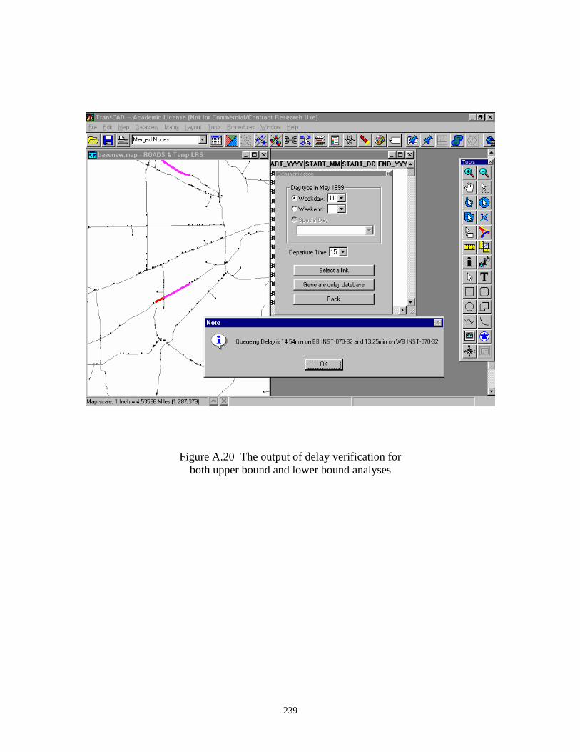
239

Figure A.20 The output of delay verification for both upper bound and lower bound analyses

240

Figure A.21 The dialog box for inputting the file name for delay database

241

Figure A.22 Dialog box for creating a new Access database

242

Figure A.23 Dialog box for importing a dBaseIV database

243

Figure A.24 An example delay database

244

Figure A.25 Input menu for TransCAD GISDK interface in project scheduling subsystem

245

Figure A.26 Schedule management menu for TransCAD GISDK interface in project scheduling subsystem

246

Figure A.27 The existing records in the scheduling database are shown in a new table and on the map

247

Figure A.28 Scheduling evaluation menu in project scheduling subsystem

248

Figure A.29 The total delay of a specific period of time

249

Figure A.30 Framework of the web access interface

HTIS web access main menu

Submit Reset

Possible Delays of links under construction

Zoom in (Click on map)

View details (Click on icon)

Re-submit


250

Figure A.31 User’s interface for travel information access subsystem

251

Figure A.32 Output screen for travel information access subsystem

A Highway Travel Information System: Forecasting and ...

Documents

Transcript of A Highway Travel Information System: Forecasting and ...