Noisy images edge detection: Ant colony optimization algorithm
A Hierarchical Layout Algorithm for
Drawing Directed Graphs
Jason Reynolds
A thesis submitted to the
Department of Computer and Intormation Science
in conformity with the requirements for
the degree of Master of Science
Queen's University
Kingston, Ontario, Canada
April, 1997
copyright 0 Jason Reynolds, 1997
Nationd Library BiblimtMque nationale du Canada
Acquisitions and Acquisitions et Bibliographic Sewices services bibliographiques
The author has granted a non- exclusive licence allowing the National L i i . of Canada to reproduce, loan, distri'bute or sell copies of hismer thesis by any means and in any form or format, making this thesis a e l e to interested persons.
The author retains ownership of the copyright in hismer thesis. Neither the thesis nor substantial extracts fiom it may be printed or otheMlise reproduced with the author's permission.
L'auteur a accord6 m e licence non exclusive pennettant a la BlaliothQge nationale du Canada de reproduke, p d k , distni.i.uer ou vendre des copies de sa these de quelque mani&e et sous qpe1que forme que ce soit pour mettre des exemplaires de cette these a la disposition des persomes int&ess&s.
L'auteur c o m e la propriktte du h i t #auteur @ protege sa these. Ni la these ni des extraits substantiels de celle-ci ne doivent &re imprimes ou autrement repoduits sans son
A significant problem with h i m h i d l a m drawing algorithms for directed graphs is
the inability to draw large graphs we& in a reasonable amount of time. This paper
d e s c r i i an extension to the algorithm presented in [GKNV93] that improves efficiency
dramaticallyY By adding a pre-prooessing step to th algorithm, a hewistic can be used to
modify the structure of the initial input graph, These m&cations automatically improve
the efficiency ofthe algorithm in [GKNV93] while still producing hierarchical layouts of
equal or better quality-
Thesis Supervisor: Dr. D. Rappaport
Title: Associate Professor
Table of Contents
ABSTRACT
TABLE OF CONTENTS
LIST OF TABLES
LIST OF GRAPHS
LlST OF FORMULAS
LlST OF INTEGER PROGRAMS
LIST OF FIGURES
CHAPTER 1 - lNTROOUCllON
1.1 Overview
1.2 Motivrtioa for this algorithm
1.3 Proposed Atgorim
CHAPTER 2 - REVIEW OF TERMINOLOGY
2.1 Graph Tedndogy
2.2 Graph Drawing Termindogy
CHAPTER 3 - LITERATURE REVIEW
3.1 Sugiyama, Tagawa and Toda
3.2 Gammer, Koutmf- North and Vo 3 -2.1 - Breaking Cycles 3.2-2 - Rank Assignment 3.2-3 - Minimizing the Number of Edge Crossings 3 -2-4 - Positioning of Vertices
CHAPTER 4 - ASSIGNING &VALUES TO EDGES
iii
CHAPlER 5 - RESULTS
5.1 Inmdmcth
5.2 Objcctivr M e m m - AedWa
5.3 Objective Meamma - E f f i
5.4 Compdmn with Pllbbkd Redta
5.5 Campuiroa of Dot and Elatdag
5.6 Summary - byoat
5.7 Efficicacy
5.8 Obst~tioaS - E f f i
CHAPTER 6 - ANALYSIS
6.1 Dmermcc in Edge Crossiags
6.2 E f f i n c y
6.3 Bumping
CHAPTER 7 - CONCLUSIONS
APPENDIX - TABLES
APPENDIX - LAYOUTS OF RANDOM GRAPHS
REFERENCES
VITA
TABLE 1
TABLE 2
TABLE 3
TABLE 4
TABLE 5
GRAPH 1
GRAPH2
GRAPH 3
GRAPH 4
GRAPH 5
GRAPH 6
FORMULA 1
FORMULA 2
List of Tables
List of Graphs
List of Formulas
List of Integer Programs
INTEGER PROGRAM 1
m G E R PROGRAM 2
INTEGER PROGRAM 3
List of Figures
vii
Chapter l - Introduction
Curreatly there are many applications that use directed graphs to represent
idormatiom ER dirgnms show the relations in a m. PERT disgrams reveal
dependencies in a specific pmject. An internet web site contains poimas to hundreds and
even thousands of web pages- Research over the last fifteen years has tried to dmlop
automatic methods for creating pictures ofthese types of appficatiom. One ofthe most
common methods is to create a hierarchid layout ofthe gcepb In this case, vertices of a
graph are assigned to levels so that all edges point in the same direction-
There are many published hierarchical graph drawing algorithms but they either
need human intenrention, work well for graphs with certain properties or M too slowly to
be acceptable solutions for the general problem.
This thesis presents an algorithm for generating straight-line planar drwviags of
directed acyclic grapbs that tries to deal with these issues. The algorithm is a modification
to the one presented in [GKNV93]. It takes a description o f a directed graph and assigns
the nodes and edge paths to a set of Cartesian co-ordi~ates~ It also introduces the use of
flat edges into the drawing- A flat edge is defined as an edge between two nodes that exist
in the same level of a hierarchy. By introducing an initial pre-processing step aad the
notion of flat edges, to the solution in [GKNV93], the efficiency of the algorithm is
dramatidy increased while layouts of equal or higher quality are produced.
This thesis is d ~ d e d into seven chapters. The first is the introduction It gives an
overview ofthe thesis, de~cfi'bes the motivation, d the general ideas behind the
algorithm. The second chapter reviews basic tamiaology used in this thesis- The third
looks at previous work done in this area ofdirected graph drawing. The f d d e s c r i i
the proposed algorithm in detail. The emphasis will be placed on describing the two
heuristics used to moday the results of[GKNV93I7s work. The fifth chapter shows the
resuits of the paformaace ofthis algorithm, wbile chapter six presents an analysis ofthese
results- In particular the quality and the efficiency ofthe d t s tiom this algorithm will be
compared with those of [STT8 I] and [GKNV93]. The final section discusses future
extensions to the algorithm aad open problems in hierarchical graph drawing-
1.2 Motivetion for this algorithm
There are many ways of representing information. A graph, G, represents the
relationships between objects- Objects are represented as vertices and their relationships
are represented as edges. A f d y tree is a typical graph. People are the vertices and their
parent - child relationships are the edges.
In computer science, there are many well known applications that can be modeled
by graphs. Computer networks form graphs. Computer terminals and servers are
considered vertices while edges represent the physical connections between them. In
objectsriented programming, software engineers use graphs to show how functions,
procedures and data structures are related to one another within a program. The internet is
dso one huge graph. Every web site is a subgraph of the entire idiastructure of the net.
Each hyper-link is an edge to another web page or node. There are many other examples
but the basics always remain the same. Vertices are connected via an edge to show that
there is some relation between them.
In order to d d with luge graphs a d the infodon they convey, buman beings
prefm to v i s d k them. Tbe layout ofany given graph caa asskt with this visualization In
particular, by laying out a graph in a specific umy, many Snterestiag properties may be
revealed. However., finding these properties md visualizing than nadily is a very difficult
problem. Because graphs m tbdt general form ban no geometric properties, there are an
infinite number of ways that they can be drawn. Thus in the past twenty years there has
been a significant amount of research done on developing algorithms which are efficient
and produce "good" layouts.
A good layout d e p d s on the aesthetics of a drawing. Aesthetics are geometric
properties that are applied to the graph in order to create a visual representation.
Aesthetics include coDstreints on the length and shape of edges, the llliaimal and maximum
distance between vertices, the Ehape of vertices and the ovdf topology ofthe graph.
How well an algorithm produces a layout with respect to these aesthetic criteria is a
measure of how "'goodn the layout is.
UnfortunateIy this may not be as straight forward as it seems. In many cases
aesthetic criteria overlap. For example a layout that msudmizes the amount of symmetry
may not necessarily minimiEe the number of edge crossiags. Lfboth these criteria are
desired, a compromise or a ranking of importance must be found. Furthermore maximizing
or minimizing the degree of artah criteria may be computationally intractable. It has been
proven then finding maximum subgraphs with symmetry is NP-complete. In general this
entire problem becomes subjective. It is the user who ultimately defines what
characteristics are important to be shown in a layout. This has kd to many algorithms
designed specifically for special cases of graphs. This thesis looks at the general problem
of drawing directed graphs.
Directed graphs have a very important property. Edges have a direction. Ensuring
that edges point in the same general direction is an important aesthetic criterion when
drawing digraphs. This has led to the development of hierarchical drawing algorithms. The
idea of a hierarchical drawing is to orient edges so that they point in the same direction, in
order to create a hierarchy ofinfomation Obviously not all directed graphs can be drawn
perfectly in this fshion but it does form a simple model
Another important resthetic criterion is avoiding visual anomalies that do not
convey idbtmafioa about the graph Tbis u d y takes the form of minhniring the number
of edge crossings ad m h h i h g the number of beds in edges. Edge crossings clutter the
graph and make it difl6dt to see which vertices are comected. A tbird criterion is to keep
edges short. This improves the readability ofa graph Edges that are short make it easy to
see which vertices are adjacent to each other. Another criterion is based on the idea of
balance. If a graph has its vertices Mnly distributed throughout the picture, a dcswiag is
considered more organized and well spaced. This results in a picture that is easier to read.
Most algorithms in the literature do not take this in tr, account. For example [STT81] does
not deal with it at all while it takes on a small role in [GKNV93].
The final aesthetic criterion deals with keeping a picture within the bomds of
whatever physical media is being used. For example a layout is not practical if it c a ~ o t
appear l l l y on the screen Therefore minimizing the overall area of the layout is
important. This is rarely addressed in the current literature; however, it becomes quite
critical when drawing large graphs.
A fuaher issue which is not concerned with aesthetics, is efficiency. There are few
algorithms that produce decent quality hierarchical layouts for large directed graphs in a
practical amount oftime. Large, in this case, means a graph ofa few hundred vertices and
edges. The reader will see that a graph composed of 75 vertices and 157 edges takes
nearly 12 hours to calculate a layout using the algorithm present in [GKNV93] on an
IBM RS6000 computer. This cost is unacceptable especially for a graph that is so small.
The algorithm described in this thesis attempts to deal with this issue as well as all
of the aesthetic issues described above. Its goal is to efficiently produce well balanced
hierarchical layouts that minimize the overall area.
The following sections gives a general overview of how this algorithm
accomplishes tbis task.
This thesis presents a graph drawing algorithm that is a modification of the result
presented in [GKNV93]. The idea is to improve on the qurlity ~d efficiency ofthe final
layout.
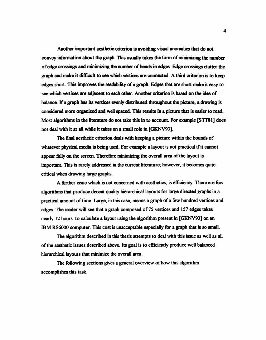
The algorithm consists ofa four stage Figure 1 - Main Algorithm process as seen in Figure 1. In the first stage, a I I. P r a p r ~ ; I
used in solving the hierarchical rank assignment t 1
pre-processing step is used to apply geometric
properties to the graph- These coostraims are then
problem in stage two. This stage finds an optimal sdution to rnhhihg the overall edge
length of the graph within the constraiats imposed by stage 1. The third stage reduces the
number of edge crossings by rearranging the order of vertices in each rank The algorithm
sweeps up and down the ranks using heuristics called the median and transpose methods
2. Rimkin@; 3. Ordering(); 4- Positioningo;
to c'smartlf' reorder the position of vertices within each rank. This continues until a global
optimum is reached. The fourth stage then fine tunes the drawing by performing local
optimization at every node. It assigns (qy) coordinates so that a compromise between the
minimkation of the overall edge length (Euclidean distance) and the "straightness" of
edges is found. The algorithm then outputs the completed drawing to a file or to a
graphid front end which displays it.
The major contributions to this algorithm are the pie-processing stage and some
modifications to the third and fourth stages. Unlike the work done in [GKNV93], not all
edges have a minimum length of 1. The pre-processing step partitions the edge set into
three subsets. These sets have a minimum length configuration of 0, 1 or 2 respectively.
This results in some edges wnnectiag vertices that have the same assigned rank. These
edges are called flat edges. The algorithm then ensures that all of these flat edges are
pointed in the same direction, preferably &om left to right across the hierarchy. Edges that
are assigned minimum lengths of 2 are used to "bump" vertices down the ranks. This
reduces the amount of overlapping or crowding of vertices in full ranks.
The addition of flat edges not only improves the quality of layouts in some cases
but also increases the performance of the third and fourth stages. it turns out that each Bat
edge in the layout reduces the overall edge length ofthe graph by at least one, when
dealing with the hnal two steps. Thus by maximidng the number of flat edges, the
algorithm is amxhkbg its &ciency- The notion of "bumping" was introduced to fix the
problem of too many flat edges. These two ideas will be demonstrated later on in
this thesis.
Chapter 2 - Review of Terminology
This section mfeMews some ofthe terminology used throughout this paper. The first
part defines rnaay tams that come fkom graph theory- The second part inboduces some
new refkemces that are to this paper and algorithm-
A directed graph, G, is deiiaed as a pair (V,E) where V represents a finite set of
vertices (sometimes referred to as nodes), and E is a finite set of ordered subsets (up)
where y v E V . LfE is the edge set then an element of E is an edge. Edges may have a
defined value based on their importance with respect to the rest of the edges. This value is
called the weight. A loop is an edge (yv) where u = v.
A vertex v is adjacent to a vertex u ifthere is an edge (up), or (v,u).. We say that
(up) is incident from or leaves vertex u and is incident to or enters vertex v. Vertex u
is also refemd to as the parent ofchild v. This means that a vertex in a directed graph
also has an in-degree and an out-degree. The in-degree of a vertex is the number of
edges incident to it. The out-degree of a vertex is the number ofedges incident firom it.
The degree of a vertex is the sum of its indegree and outdegree. A source vertex is a
vertex with indegree 0, while a sink node is a vertex of out-degree 0. A neighbor, v, of a
vertex u, in a directed graph is any vertex that has an edge (u,v) or (v,u).
A path of length k from a vertex u to a vertex z is a sequence <vo, vl, v2, ... , vkl,
v p of distinct vertices, except for vo and vk where vo = u and vt = z and (%, vi+,) E E for i
= 1,2, ... , k - 1. A path contains vertices vo, v,, ... , vb A path forms a cycle ifv. = vk
and the path contains at least one edge. A graph with no cycles is said to be acyclic.
A graph is connected if every pair of vertices is connected by a path. An
undirected graph has no order placed on the edges. An undirected connected acyclic
graph is said to be a tree. A unique distinguishing vertex of a tree is called its root. For
every finite undirected connected graph, G, there is a spanning tme. A spaaning tree is a
tree that includes all the vertices o f0 and uses only edges of G-
A connected directed graph is said to be hlauchkrl if it is acyclic. A vaat q is
an ancestor of v, ifthere is a path fiom u to v m a directed graph In this instance, v is a
dcsceadwt ofu. For firither idbcmation on graph terminology please refer to @UR69].
A drawing of a graph is an assipmeat of the vertices and edges ofthe graph to a
set of Cartesian cosrdiaates. Vertices are then drawn at their (qy) position and edges are
drawn using straight-lines along their pmjected (qy) paths.
A hierarchid drawing is a drawing that assip each vertex to a rank. A rank
or, equivalently a level, is a line in the plane that runs parallel to all other ranks. A
hierarchy is the composition of all these ranks. When the vertices are actually placed on
the screen, all vertices in the same levei will be placed in a line, parallel and in between the
vertices on the level above and the level below. For the purpose of this algorithm, the
distance between two vertices u and v, is defined as the absolute value of the difference
between the rank of u and the rank of v. For notation purposes the rank of v is defined by
the &action Vv). The length of an edge (up) is simply the distance between u and v- The
main goal of this algorithm is to minimize the overall edge length without having too many
vertices in any particular rank- Thus this definition is very important in understanding this
algorithm. A hierarchy is said to be proper ifall edges have a length of 1, and all
descendants of a vertex are assigned to a rank greater than its ancestor.
One problem however, is that a directed graph may have a hierarchical layout
which consists of only one rank. This results in very unsatisfactory layouts. So a minimum
value constraint is given to each edge. This is called the minimum length denoted as 6(e)
where e is an edge. It can be any integral value greater than or equal to 0. In our final
layout, all edges will have length greater than or equal to there minimum length constraint.
Another important chatact&stic ofthis graph drawing algorithm is that of edge
crossings. Two edges intersect or erog ifthe line segments repnaenting the edges
intersect. Trying to m h h k e the number ofedge crossings is highly d e l e in a good
layout.
The hyout ofa graph is the placement ofvertices and edges in order to create a
physical representation. In terms ofthe hyout or equivalently picture of a graph, a few
items need to be defined- 'Chis thesis speciscally deals with heirarchid layouts, so the
height o f a layout is defined as the total number ofranlcs. The order of a rank is the
number of vertices in it. A layout is said to have a width equal to the highest order in the
hierarchy. These tams will be used in discussing the propaties of a layout.
Chapter 3 - Literature Review
Over the last twenty years, there have been amny attempts to develop an algorithm
which provides good drawings for any general graph In most cases, they work well for
some graphs and not for others. Some typical problems for any algorithm include
unsatidktory layouts for certain graph configurations and computationally expensive for
large graphs. Many papers have ban written to address these issues; however, no one has
mme up with a solution that is s i g n i s d y better than my of the others.
The same is true ofdrwving directed graphs. S i 1977 when Warfield developed
his cCCr~ssing Theory and Hierarchy Mapping'' In wARF77I most research papas have
tried to follow his basic idea. F i i assign vertices to their proper levels in the hierarchy
and then try to minimize the number of edge crossings while still maintaining this
hierarchy. In [STT8 I], Sugjama, Tagawa, and Toda (from now on refmed to as STT)
introduced an additional aspect to the layouts. They suggested that long edges (i-e. edges
between vertices separated by > 1 level apart) should be as straight as possible. That
resulted in the addition of a third step to Warfield's original mode:. They also introduced a
new heuristic for the removal of edge crossings. This new heuristic turned out to be the
cornerstone for many research papers focused on reducing the number of edge crossings
in a hierarchical drawing. Also at this time, Carpano suggested a similar approach to
removing edge crossings [CARP80]. His method was based on an iterative solution. His
heuristic continued to run until a global minimum was reached.
Later, in 1986, Eades and Kelly showed that minimizing the number of edge
crossings in a 2 - level system is NP-complete IEADES861. This proved that the use of
heuristics for removing edge crossings was a "good" way of solving this problem. It also
seemed to reduce the emphasis on developing good heuristics for the removal ofedge
crossings and led to a broader view of graph drawing-
At this time Battista, and Tamassia @3T88] presented an O(N log N) algorithm for
drawing planar directed acyclic graphs. Its limitation, however, is that it only works for st-
graphs. An st-graph is an acyclic digraph that has one source node, s, and one sink node, t,
and there exists an edge (s,t). In 1994 Bertolazzi, Liotta, hhmho pBLM.941
extended this, to test whether a 3-reguhr acyclic digraph bas an upward planar drawing in
O(n+?) thewherenis thenumbetofvfftices, ad ris thentmberofsou~cemd sink
nodes. An upward planar drawing is simply a hierarchical drawing with no edge crossings.
These results show that for specific types ofgraphs, there exkt &st algorithms that
produce good laputs, but fix large general directed graphs the have yet to be my
significant improvements.
In the late ~ O ' S , algorithms for drawing small graphs with good layouts were quite
commoa So researchers looked to the problem of drawing large graph fkom a d
graph point of view. The basic thought was that by breaking up the graph into smaller
parts, large graphs d d be drawn by finding good layouts for the small grapbs, and then
incorporating these small layouts into one large one. In 1991, Messinger, Rowe and Henry
presented a divide and conquer approach in -11 based on this idea Their results
however showed that the divide and conquer approach to graph drawing is not a good
one. The rnain reason for this is the quality of the final layout. Individual subgraphs may be
well drawn, but when incorporated with the rest ofthe graph, the picture looks awkward
and messy. This can been clearly seen in instances where there are numerous edges
connecting each subgraph. The idea ofgrouping sets of vertices togaher comes tiom the
work of Gestalt [GEST47]. His theories on grouping in terms of perception have lead to
many algorithms including a rule-based approach to layouts P S 9 4 1 , and a recursive
clustering method WORTH931. The problem with both of these solutions is that deciding
which set of vertices constitute a subgraph, is extremely difticult. In both of these
algorithms, the assumption is mde that these subgraphs are determined m a a d y or by
some external device-
North's basic algorithm came fkom a paper he w-authored in the late 80's
[GKN88]. In it, an algorithm was presented that produces layouts where the assignment of
levels in a hierarchy is optimized so that the overall edge length in the graph was
Then in 1993 he co-authored another paper based on the earlier one
[GKNV93]. Here, the initial algorithm was extended so that curves were used to represent
edges and the '"straightness" of the edges was optimized.
Amther approach is to a a t e a chtbase of drawing algorithm, and then to
automatidy choose which dgorithm wwM be best suited to draw a particular graph,
This was done in [BBL95]. The one problem with this method however, b the amount of
human intefveLnion aeeded to decide the bat suited algorithm to produce the best picture.
Tba am muy digraph drawing algorithms but most oftban follow the same
basic strat Jes tht are shown above. The ideas presented in this paper are based on the
algorithms contained in [GKNV93]. For a more in depth review, the reader is refa to the
annotated bibliography in @ETT94].
The next section looks specifically at 2 different approaches to drawing direzted
graphs. The fint will discuss S' ITs work and how it affied many papers that followed.
The second is a look at Gansner el d ' s "A Technique for Drawing Directed Graphs"
[GKNV93] and the iimitations that it preseuts.
3.1 Sugi'ma, Tagawa and Toda
Most recat algorithms that draw
directed graphs in a hierarchical way are based
on the ideas that were proposed in their paper in
198 1 [STTS I]. Figure 2 shows their 4 step
process in which a description of a directed
Figure 2 -
1. Transform into hierarchy. 2. Reduce edge crossings. 3. Horizontal Positioning of
vertices- 4, Display on terminal.
graph was input and a picture of the graph was the resulting output. The aesthetic goals of
this algorithm are to orient edges in the same direction, minimize the number of edge
crossings, and to keep edges short and straight.
The first step was to transform the graph into a proper hierarchy. STT do not go
into details about how tbey do this but it is inferred that all cycles are eliminated by
reversing the direction of some of the edges and all edges that span more than I level are
replaced by a series of dummy vertices and edges. This ensures that the graph is a proper
hierarchy.
The second step was to reduce the rmmba of edge crossings in the g n p h Once
the hierarchy was fix&, an orderingwas imposed on the in each level. Thedbre
a vertex in level i was assigned to some position with respect to the other vertices in the
same level. By modifjring the order for each level, the number of edge crossings in the
graph can be reduced in most cases- The heuristic they used ans called the ~ e n m c
methad The basic idea is as follows. Starting at level 2 aad continuing to kvd k (k being
the maximum level) each vertex in a level is 8SSigued a position based on their ancestors in
the level above. This position is calculated as the avefage of the positions of a vertex's
ancestors in the previous rank. They are then sorted based on their new position values.
Once this has been completed for all levels the number of edge crossings is calculated for
the entire graph and this is compared with the previous due. The algorithm sweeps up
and down the levels until then is no more improvement in the number of edge crossings.
Once this has been completed, the problem of assip& actual (qy) coordinates
to the vertices is solved using a heuristic called the Priority Layout Method. The basic idea
is to make edges as straight as possible. Therefore long edges which are composed of
dummy vertices will be relatively straight and easier to read. The process is similar to the
barycentric method discussed above. By starting at level 2 and iterating through until lwel
k, each vertex in each level is assigned an integral x co-ordinate. These coordinates will
maintain the ordering imposed by step 2. Which vertex is the next to be assigned an I co-
ordinate is based on its priority number Dummy vertices are given higher priority than
non dummy vertices because they compose long edges. Because dummy vertices have an
in-degree of 1 they can be placed directly below their ancestor. AU other vertices are
assigned x wsrdinates based on the integral average of their ancestors. If these values
break the constraints of the imposed ordering then they are inserted as close as possible
without breaking any of these constraints.
The final step reverses all previously reversed edges, removes dummy nodes, and
outputs the final layout onto the saeen
This algorithm is fast and works quite well, however there are many areas that can
be improved upon First of all, the problem of partitioning the set of vertices into levels is
never explicitly addressed. In fact very tittle work appears in the literature about this

problem Most research tends to deaf with the edge crossing probletn more than setting up
the organization ofthe hierarchy. One ofthe kdati011~ that this algorithm has is that
edges may be but sometimes mmxmdy long. This results in more dummy
nodes than needed a d tberefbre the computational time is greater. Furthermore, the edges
sometimes have sharp beds as thy leave or enter d e s . This is undesirabIe becase it
makes reading the graph more diflEicult. Another ObsaMtion is that in most drawings the
perimeter is unnecessady huge. This means that the widtbmcight ratio becomes extreme
(i.e. one of the width or height is much greater than the other), and screen limitations start
to interfere with the o v d quality ofthe layout. Tbis becomes a &tor when Bcaliag is
needed. Any layout can be scaled down to fit on the screen, but to ensure the layout is
unchanged, the scaling must be done by a constant &tor. M o r e if either the height or
width is much greater than the other, the final layout wilI be d e d down much more than
necessary. Individual vertices m y start to overlap one another or entire levels will become
scrunched together, thus making reading the graph more difficult than necessary.
The next section looks at another algorithm that is similar in design but specifidy
looks at solving the level assignment problem and ( ~ y ) assignment problem
3.2 Gansner, Koutsofiao, Norfh and Vo
Like STT's algorithm, Gansner et d.
propose a 4 step algorithm that draws a directed graph in
a hierarchical layout as seen in Figure 3. This algorithm
differs in two distinct ways fkom the STT algorithm It
explicitly solves the level assignment problem such that
the overall edge length of the graph is minimal and all edges have similar orientation. It
also maximizes the "straightnessn of all edges within the graph Moreover, because their
implementation uses curves to represent edges, their algorithm tries to avoid sharp bends
as much as possible.
The first step ensures that the graph is acyclic by reversing a subset of edges. Then
the hierarchy is found by solving the following mathematical formulation: minimize the
overall length such that an ancestor of a vatat h y s appears in a lower I d than its
descendent They sdve it using a network simplex approach Even though this type of
solution is not proven to be polynomial, in practice it nquires vay few iterations even on
graphs composed of 250 vertks.
The second step is similar to STTs. By npkcing edges that separate vertices more
than one l e d apart with a comected chain of"vir&dw or dummy vertices, an ordering
can be imposed on each level. By manipulatiag this order, the number of edge crossings
can be demased. Gansner et PI. propose two modifications on existing heuristics called
the median and transpose methods. They are claimed to work 20-50% better than the
barycentric method.
The third step is to assign (&y) coordinates to each vertext By applying the same
algorithm as in step L to a specially transformed graph, an optimal solution can be found
to the problems of keeping edges stratgght, minimirjng edge length and avoiding sharp
bends. The problem however is that this transformation results in a much larger graph, and
the domputational time becomes much more! expensive.
The final step computes the curves that will represent the edges. For each edge a
set of control points are calculated such that the curve they represent is as smooth as
possible and yet avoids all obstacles like other nodes and edges. The control p o h s will
then be used to draw piecewise Bezier curves. The results of using cuwes instead of
straight-lines are aesthetidy pleasing but does not improve on the overall readability of
the graph.
This algorithm is a drastic improvement on many of the areas that STTs algorithm
lacked. It does have its problems as well. In some cases, it is sometimes desirable to have
longer edges. When there are a large number of vertices in a single level, it is better to
spread them out among more than one level. This is particularly beneficial if one of the
adjacent levels has few vertices. Also, the third step can become quite slow depending on
the size ofthe graph. Thus, even though this algorithm is optimal with respect to
minimizing the total edge length of the graph, it still does not necessarily produce a
"perfectn drawing. In most cases, a drawing that minimizes the total area of the graph is
better than one that minimizes the total edge length.
Because the algorithm descriii in this paper uses the algorithm pnscdtd in
[GKNV93] explicitly, the fouowing sections will describe it in detail.
By definition a hierarchy has no cycles A directed graphs, however, am have
cycles. So before vertices can be assigned raDLs properly, aU cycles must be eliminated
&om the graph. To deal with this problem, some pre-processing is done that detects cycles
and breaks them by reversing certain edges. It should be noted that this is done internally
and that when drawn, these edges will have their original direction There are a number of
ways that this can be accomplished but it tuns out that the simplest way is diicient. By
doing a depth-first search starting fiom a source node, if it exists, a partial order is defined
by the depth-first search tree. The edges are then partitioned into two sets: tree edges and
non-tree edges. By incrementally looking at all non-tree edges and adding them to the
initial partial order, each non-tree edge can be placed into one of three categories: cross
edges, forward edges or back edges. Cross edges comect unrelated nodes in the partial
order while forward edges connect an ancestor to a descendant. These types of edges
when added to the partial order do not create cycles. Back edges, or edges that connect a
descendent to its ancestors, do create cycles. By reversing a back edge, one creates a
forward edge. So by reversing evexy back edge, all cycles are broken.
What is important to note is that in some cases by breaking cycles in this manner, a
large number of edges may be reversed depending on the graph input. Hence, when the
actual drawing is wormed there will be a large number of edges pointing in the opposite
direction to the rest ofthe edges in the graph One way of dealing with this is by reversing
the minimal set of edges in the graph so that no cycles occur. This however, is the same as
solving the feedback arc set problem which is NP-complete [EADES86]. So solving this
problem in this manner is computationally unacceptable. It tuns out that the depth-first
solution in most cases works effectively as well as quickly.
As stated eartier, the ranking part ofthe dgoritbm tries to minim& the
sum of the over aU edge length in the digraph while m h a i n b g a hierarchy. Recall that
the length ofan edge (v.w) is A(w) - Mv) where u w ) cpuals the Rnlr ofvertex w. Then the
hierarchical property of the graph can be edorced by having all edge lengths greater than
the miaimurn length comtnht 6(v,w). Therefore the folfowing is a mathematical
formulation of minimizing the sum of the o v d edge length for a hierarchical layout.
Integer Program 1
subject to: R(w) - R(v) 1 6(v , w)V(v, w) E E
The weight o of an edge (v,w) is used to give a higher priority to special edges. In most
cases the weight of an edge is equal to 1.6 is the minimum length h c t i o n and is used as a
vertical positioning constraint. It ensures that the hierarchical property ofthe layout is
maintained, when 6(v, w) > 0.
Now, we have a linear objective
function that is subject to a system of linear
constraints, that is, a linear programming
problem. There are known ways of finding
an optimal solution to this problem in
polynomial time; however, as in
[GKNV93], a good method of solving it is
called a network simplex. This has not
Figure 4
1- init-ranko; 2. feasible-tree(); 3. while (e is an edge with cutvalue < 0) 4. f = replacement edge for e; 5. exchwiF(e,f) ; 6. end 7. nocmalize0; 8. balance();
been proven to be polynomial but for this problem tends to work using very few iterations.
A brief description can be seen in Figure 4.
The basic theory behind a network simplex solution is to find an initial feasible
solution, and then txy to improve on it by increasing one variable at a time. A solution is
f-Me if it l ia within dl coastraints imposed in the initial problem In tamr of
minim&g the sum of the o v d edge length, all edge lengths must be greater than or
equal to their minimum length coastniat. How ht a solution is from the optimaI is
measured by a series of slack wuiables. Note tbat the slack variables in this caae are
d&ed as the length ofan edge mimw its miainum length 00aStraint. An edge is
considered tight if its slack is 0. As the slack variabIes deaease in value because of the
increase in the other mkbles, th closer the fe851ile solution becomes to the optimal one.
However, when an increase in any ofthe variables will make the solution infie8~1%1e, the
solution is coosidered opt id . As a rule, the choice of which variable to be increased in
each iteration is based on what vbable will move the solution closest to an opt'unal
solution It is then increased as much as possible so that its new vaIue will still induce a
feasible solution Tbis is continued until the optimal solution is reached. This is obviously a
simplified explanation but it will suffice for the purpose of descriing how the rankiog
assignment works. For more information on this type of solution the reader is referred to
WST831.
So how can this type of solution be applied to this graph problem? It is in fact very
simple.
The first step (lines 1-2) of Figure 4, is to construct an initial feasible solutioa. This is done
as follows.
Figure 5
1. white(Vt(})do 2. for all v E V with no "in" edges 3. AssignRank(v); 4, delete v and a l l its edges. 5. end for 6. end while
In other words, each source vertex is assigned a rank then deleted from the graph (lines 2-
5 of Figure 5). A vertex v is assigned a rank based on the following formula.
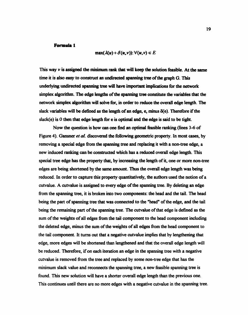
This way v is assigned the minirmm rank that will keep the sohmon feasible. At the same
time it is also easy to construct an undirected spmhg tree of the graph G. This
underlying undirected spanning tree will have important implications for the network
simplex algorithm, The edge iengtbs ofthe spanning tree constitute the variables that the
network simplex algorithm wiIl solve for, in order to reduce the overall edge iength. The
slack variables will be defined as the Iength of an edge, e, minus 60. Therefore if the
sIack(e) is 0 then that edge length for e is o p t i d and the edge is said to be tight.
Now the question is how can one find an optimal ksi i Ie ranking (lioes 3-6 of
Figure 4). Gansner et ul. discovered the following geometric property. In most cases, by
removing a special edge fiom the spanning tree and replacing it with a non-tne edge, a
new induced ranking can be constructed which has a reduced overall edge length. This
special tree edge has the property that, by increasing the length of it, one or more wn-tree
edges are being shortened by the same amount. Thus the overall edge length was being
reduced. In order to capture this property quantitatively, the authors used the notion of a
cutvalue. A cutvalue is assigned to every edge ofthe s p a ~ i n g tree. By deleting an edge
f?om the spanning tree, it is broken mto two components: the head and the tail. The head
being the part of spanning tree that was connected to the "head" ofthe edge, and the tail
being the remaining part of the spanning tree. The cutvalue of that edge is defined as the
sum of the weights of all edges fiom the tail component to the head component including
the deleted edge, minus the sum ofthe weights of all edges fiom the head component to
the tail component. It turns out that a negative cutvalue implies that by lengthening that
edge, more edges will be shortened than lengthened and that the overall edge length will
be reduced. Therefore, if on each iteration an edge in the spanning tree with a negative
cutvalue is removed from the tree and replaced by some non-tree edge that has the
minimum slack value and reconnects the spanning tree, a new feasible spanning tree is
found. This new solution will have a shorter overall edge length than the previous one.
This continues until there are no more edges with a negative cutvalue in the spanning tree-
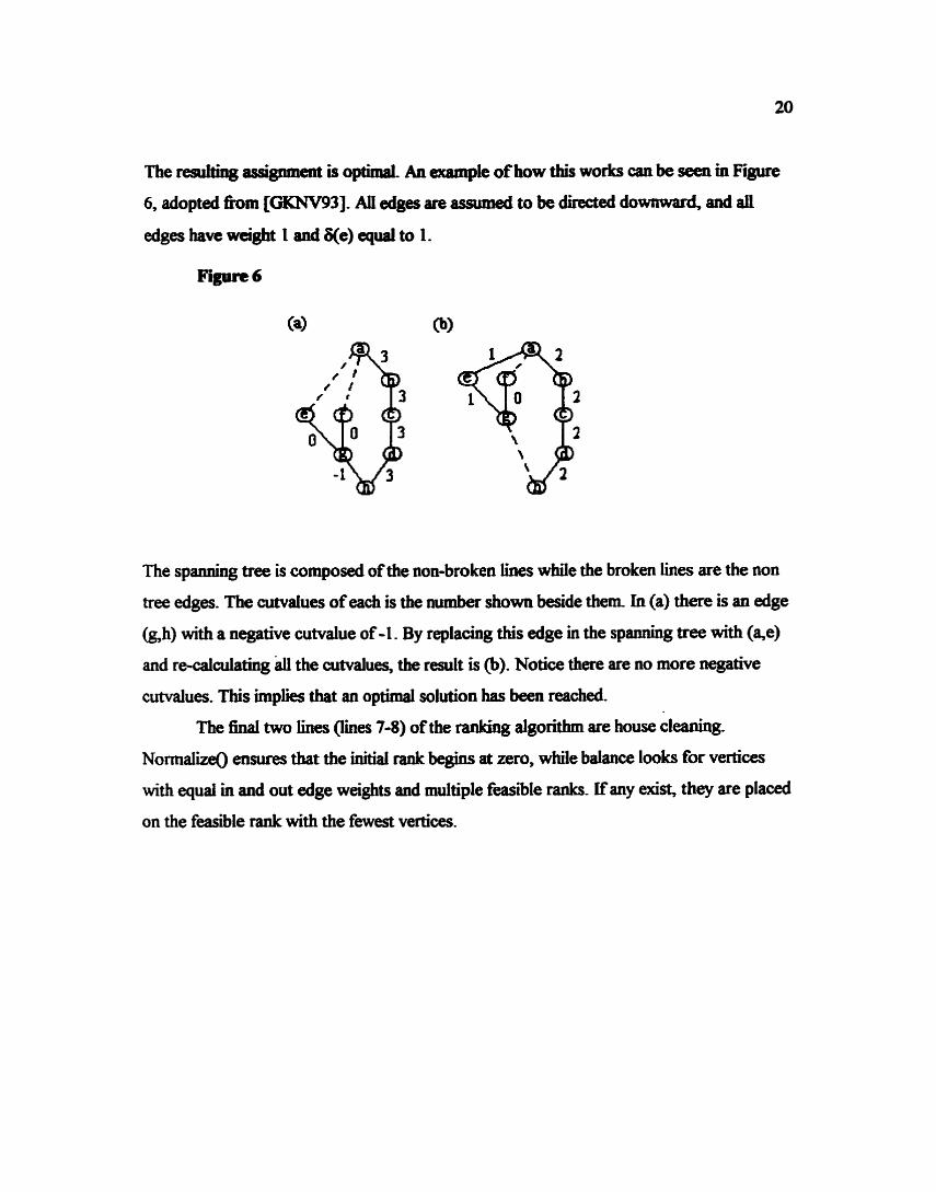
The resulting assignment is optimeL An example of how this works cau be seen in Figure
6, adopted h m [GKNV93]. An edges are assumed to be directed downward and all
edges have weight 1 ead 6(e) equal to 1.
The spanning tree is composed of the noa-broken hes while the broken lines are the oon
tree edges. The cutvdues of each is the number shown beside them In (a) there is an edge
(gh) with a negative cutvalue of-1 . By replacing this edge in the spanning tree with (a,e)
and re-calculating dl the wtvalues, the result i s Q). Notice there are no more negative
cutvalues. This implies that an optimal solutiou has been reached.
The final two lines (lines 7-8) ofthe tanlting algorithm are house cleaning.
Normalize0 ensures that the initial rank begins at zero, while balance looks for vertices
with equal in and out edge weights and multiple feasible ranks. [f any exist, t h q are placed
on the feasible rank with the fewest vertices.
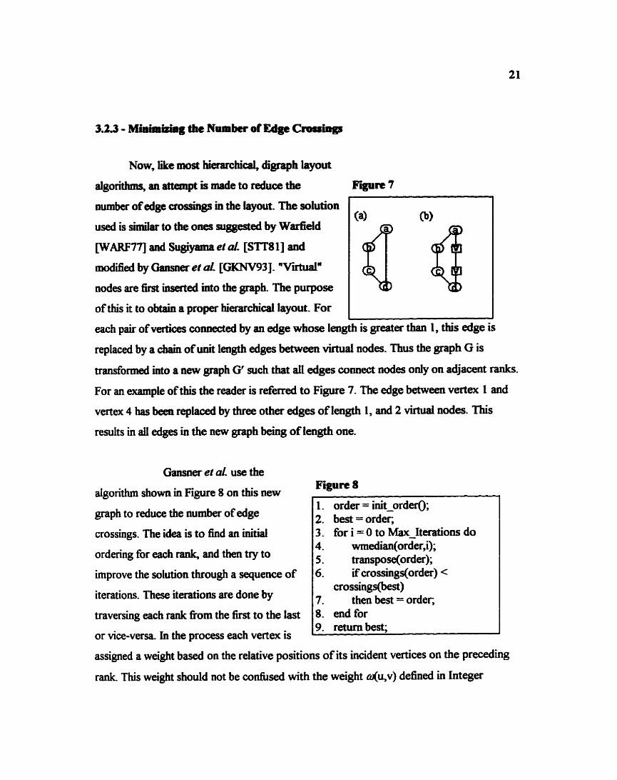
Now, like most hierarchical, digraph layout
algorithms, an attempt is mde to reduce the F i i rc 7
vertex 4 has been replaced by three other edges of length I, and 2 virtual nodes. This
results in all edges in the new graph being oflength one.
number of edge crossings in the layout. The solution
used is similar to the ones suggested by Warfield
[WARF77] and Sugiyama et d [SITS I] and
modiied by Oansner et al. [GKNV93]. " V i i "
nodes are first inserted into the graph. The purpose
ofthis it to obtain a proper hierarchical layout. For
Gansner et al. use the
algorithm shown in Figure 8 on this new
graph to reduce the number of edge
crossings. The idea is to find an initial
ordering for each rank, and then try to
improve the solution through a sequence of
iterations. These iterations are done by
traversing each rank from the first to the last
or vice-versa In the process each vertex is
(a1 @)
d
Figure 8
1. order = init-order(); 2. best = order, 3. for i = 0 to MaxJterations do 4. wmedian(0rder.i); 5. transpose(order); 6. ifcrossings(order) <
crossings@est) 7. thea best = order, 8. end for 9. return best;
each pair ofvertices connected by an edge whose length is greater than 1, this edge is
replaced by a chain of unit length edges between virtual nodes. Thus the graph G is
trdormed into a new graph G' such that all edges connect nodes only on adjacent ranks.
For an example ofthis the reader is referred to Figure 7. The edge between vertex 1 and
assigned a weight based on the relative positions of its incident vertices on the preceding
rank. This weight should not be confused with the weight 4 y v ) defined in Lnteger
Program 1. A weight is assigned to each vertex, not to any ofthe edges. A new ordering
for each raak is found by sorting the vertices by their weight.
The iaitial ordering (line 1) is done using a simple bread^^ search, By starting
with vertices of lllinimum rank, vertices are placed in their raaks in left to right order as
the search progresses- A depth-first approach could also be used in this manner. This way
trees will have no iOitial edge crossings by c~os~ruction.
To deal with calculating the weights tbr each vertex (line 4), a variation ofthe
median heuristic is used. The median method was first developed by Eades and W o d d
in 1986 [EADES86]. The basic idea is create a List of the positions of all incident v d c e s
on the foliowing rank, and to take the median ofthis list as its weight. In the case that
there are two medians (i.e. the length of the List is even), the value ofthe median that
places the vertex closer to the side where its children are more densely packed is used.
The hope is that by placing a vertex near to more of its children, the number of edge
crossings will be fewer. In fact, it was proven that the number of edge crossings will be no
more than 3 times the minimum number ofcrossings in a two level layout by using this
heuristic. However, this upper bound is still f&ly high, so like in [GKNV93], an additional
heuristic is used.
The transposition heuristic (line 5) switches neighboring vertices within a rank, and
checks to see ifthere has been an improvement in the number of crossings. Ifthere has
been, another two vertices are switched. This continues until there is no more
improvement. By starting at the lowest rank and working downwards, Gansner et ai. claim
that there is an additional reduction in the number of edge crossings by 20-500/o. The
reason for this, is that the median method only gives an approximation for the best spot to
place a vertex in the ordering. The transpose method then checks to see if positions
around the given one may be better in order to reduce the overall number of edge
crossings.
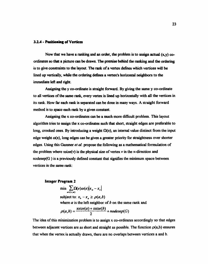
3.2.4 - Positioning of Verticts
Now that we have a ranking and an order, the problem is to assign actuai (qy) co-
ordinates so that a pictun can be dnwa The premise behind the ranking and the ordering
is to give constraints to the layout. The rank of a vertex defines which vertices will be
lined up vertically7 while the ordering defines a vends horizontal neighbors to the
immediate left and right.
Assigning the y co-ordinate is straight forward. By giving the same y coordinate
to di vertices of the same rank, every vestex is h e d up horizontally with afl the vertices in
its rank. How far each rank is separated can be done in many ways. A straight forward
method is to space each rank by a given constant.
Assigning the x co-ordinates can be a much more difficult problem. This Iayout
algorithm tries to assign the x wadinates such that short, straight edges are preferable to
long, crooked ones. By introducing a weight R(e), an internal value distinct fiom the input
edge weight ge ) , long edges can be given a greater priority for straightness over shorter
edges. Using this Gansner et rrl. propose the following as a mathematical formulation of
the problem where xsize(v) is the physical size of vertex v in the x-direction and
nodesep(G ) is a previously defined constant that signifies the minimum space between
vertices in the same rank:
Integer Program 2
Inin C W w ( e ) l x , - x"( e=(v*w)
subject to: x, - x, 2 p(a,b) where a is the left neighbor of b on the same rank and
The idea of this minimization problem is to assign x co-ordiiates accordingly so that edges
between adjacent vertices are as short and straight as possible. The function p(a,b) ensures
that when the vertex is actually drawn, there are no overlaps between vertices a and b.
Having adjacent vertices aligned vectically d t s in shorter edges. Tbir alignment
corrzsponds to reducing the horizontal distance between adjacent nodes. It is particularly
important to have vinud nodes aligned vertically so that edges pn straight. Iftbis is not
done, the edges become "spaghetti-like." This is the mnin plrpose for the wnstrPiat n(e).
By setting Q(e) equal to 1 for edges between two real nodes, equal to 2 for edges between
a real node and a virtual node, and equal to 8 for edges bctwcea two virtual nodes, it
becomes more important to straighten long edges over short ones.
The above hear propaning problem is analogous to the rank assignment
problem. The idea is that x co-ordinates can be considered as "ranks". By replacing every
edge e = (UJ) in G by a vertex a, aml two edges (b,u) and (Q& a new d a r y graph is
created. The minimum length coostraiat 6 for these edges is 0 and they have a weight, Q =
o(e)Q(e). The addition of these new nodes and edges allow for the x assignment problem
to be thought of as the ranking problem.
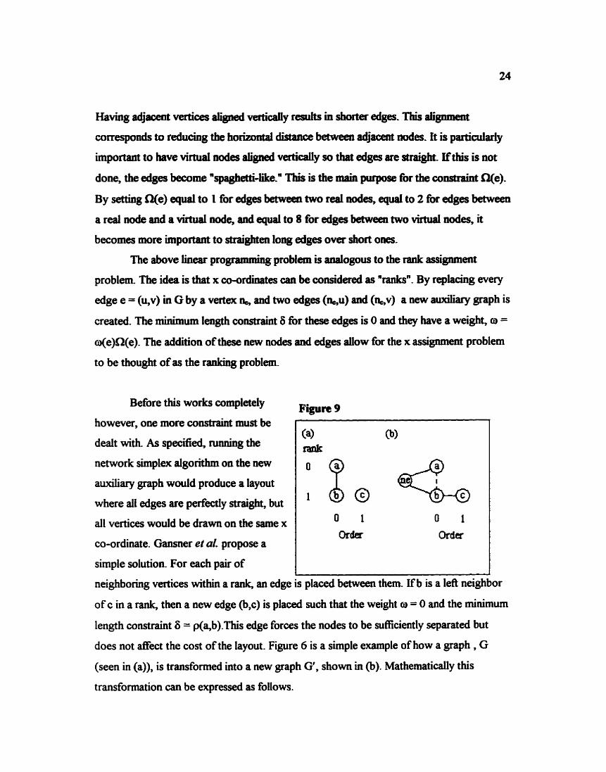
Before this works completely
however, one more constraint must be
dealt with. As specified, running the
network simplex algorithm on the new
auxiliary graph would produce a layout
where all edges are perfectly straight, but
all vertices would be drawn on the same x
co-ordinate. Gansner et al. propose a
simple solution. For each pair of
Figure 9
0 1
Order
neighboring vertices within a rank, an edge is placed between them. If b is a left neighbor
of c in a rank, then a new edge @,c) is placed such that the weight o = 0 and the minimum
length constraint 6 = p(a,b).This edge forces the nodes to be sufficiently separated but
does not atfect the cost of the layout. Figure 6 is a simple example of how a graph , G
(seen in (a)), is transformed into a new graph G', shown in (b). Mathematically this
transformation can be expressed as follows.
LetGP=(Vu V', El vE2).ThevatstsetV' contakaaewvertexneforevery
edge ecG. The edge sets El and E2 are given by El = (( ne,u),( ne,v) where (up) E G}
and E2 = ((v,w) where v is the left neighbor of w in the same rank) and all have weight
o(u,v). Now we can express Integer Program 2 in tenas of G'.
en C a r ( v ~ . l ( w ) - 4m .=(v,w)E@
subject to: ( Z w ) - (A@)) r 6(v, w)V(v,w) E EI where cu(v, w) = 0.
and 6(v, w ) = p(v, w ) if (v, w ) E E,
The network simplex algorithm descn'bed in Section 3.2.2 can now be used to
solve the level assignment problem shown in Integer Program 3. It should be noted that
the optimal solution to the level assignment on G' is also the optimal solution to the
positioning problem on G, as shown in [GKNV93].
Proof
A solution to the positioning problem on G wrresponds to a solution of the level
assignment problem on G' with the same cost. This can be seen by assigning each
vertex n. the x-coordinate x, = min(xu,xv) where u and v are vertices connected by
the edge e, and xu and x, are the x co-ordinates of u and v. Then the cost of edges
( ~ 4 and (GP) is cu(e)a(e) (x. - X, ) + o(e)W)( xv - X, ) = NdW9l X, - xv I - Therefore the cost of a solution in G is equal to the cost of a solution in G'.
Conversely, any solution to the level assignment in G' induces a valid positioning
in G by construction Also, in an optimal level assignment one of ((ku), ( h v ) }
must have length 0 and the other would have length [xu - xvI. This means that the
cost of the original edge (u,v) equals the sum of the cost of the two edges (&,u)
and (b,v) and the solution for G' has the same cost as G. Therefore the optimality
of G' implies the optimality of G.
We have shown how [GKNV93] do hierarchical graph drawing using integer
programming problems to find optimal solutions for the ranking and positioning aspects of

their algorithm. However, these solutions are based on constraiatS that are not explicitly
dealt with. They suggest that not aii 6<e) d u e s are equal to one, but they never given any
explanation for alternative values or techniques for assigning non-unacy 6(e) values. In the
next section we address this issue.
CHAPTER 4 - Assigning &values to Edges
The mejor co~tribution ofthis thesis is a modification to the algorithm desgibed in
[GKNV93]. A prqrocessitlg step is introduced to assign non--nity S(e) values. It uses
heuristics to moday the initial properties ofthe input graph Where Gansner et al. define
the minimum length constmint to be 1, the pre-processing step partitions the edge set into
three subsets where the minimum length coastreims are either 0, 1 or 2. Edges that have a
6(e) = 0 have the possib%ty ofbecoming "flat" in the final layout depending on the results
of the rank assignment. By having certain edges in the final layout flat, the tinal layout can
potentially have fewer ranks and reduces the sum of the overaU edge length. Furthermore
if all flat edges point in the same direction (e-g- &om iefi
to right) reading graphs can be easier. Figure 10 shows
the algorithm presented in this paper. Break_CycIe@,
Ranko; and Position0 are identical to those presented in
[GKNV93]. The Preprocess0 and some modifications to
the o r d e ~ g are the contri'butio~~s of this paper to the
ideas of Gaasner et crl. This chapter will look at the
Figure 10
details of the preprocessing step, and some of the modiications needed in order for the
ordering step to deal with the notion of flat edges.
4.1 Pm-processing Figure 11
In most cases the weight of an edge is I 1. for ali source nodes, ucV I equal to 1.6 is the minimum length function and is I 2. MaximalLongestPath(u);
3. end for used as a vertical positioning constraint. Because
I I
the length of edge e = (v.w) is defined as k(w) - q v ) , the S(v,w) function ensures that the
hierarchical property is maintained, if 6(v,w) > 0. Usually the 6 fimction for all edges is
defined as 1 but in many layouts by modifying these 6 values, a better layout may be
achieved. By setting some 6 values to 0, and others to 2, a more equal distribution of
vertices occurs throughout the ranks of the graph. The question is without any initially
known properties how does one choose which edges to assign 6 values of OJ or 2? W e
propose two heuristics. One for 6(e) = 0 assignments and one For the we) = 2
assignmeats. The g d of the latter is to clean up the results of the formet- The reasom will
be discussed later in this thesis-
In order to see wbich edges should be assigned the 6 value of 0, it was observed
thet long cbains of vertices comected by flat edges are preferable to multiple flat edges
randomly placed in the drawing. Also, each vertex can have at most one flat edge entering
it, and one leaving it. Tbis way there can be no overiapping edges (edges drawn over top
of one another). So that led to the assumption that for each vertex at most one entering
edge and one leaving edge would be given a S value of 0.
The algorithm is shown in
Figure 1 1 and is descri'bed in
detail as follows. By starting at
some arbitrary source node, do a
depth first traversal such that for
each vertex u encountered, of all
the edges (up), where v has no
in-edges with 6(e) = 0, choose an
edge e = (up) that initiates a
maximal longest path Eom u and
set 6(e) = 0. The additional
constraint on v ensures that each
vertex can have at most one in-
edge and one out-edge. If there
are no such edges that meet this
requirement, then u will not be
assigned any out-edges with a 6-
value equal to 0. A nice feature of
this algorithm is that it is simple
Figure 12
im IthimabngestPath (vertex u) 1. if( Marked (u) AND No-InFlatEdges (u) ) 2. return LP(u); 3. else if( Marked (u) ) 4. return -1; 5. endif- 6. Mark@); 7. if (u is a sink vertex) 8. LP(u) = 0; 9. return 1; 10- else 11. best = -1; 12. for each edge (yv) do 13. length = MaximallongeStPath(v); 14. ifoength > best) 15. best = length; 16. bestvertex = v; 17. end if 18. endfor 19. LP(u) = best; 20. if(LP(u) 2 0) 21. G(u,bestVertex) = 0; 22. return LP(u)+ 1; 23. else 24. return 0; 25. endif 26. end if
to codee Figure 12 shows the d e ~ & of the how i t works LP@) is the length ofthe Iongest
path fiom vertex u and No-InFIatEdges(u) is a check to guaraatee that u does not have
any indges that have we) = 0. Mark(u) is a means of w g a vertex as "alndy been
seed7
This algorithm is based on the kt that the length of the longest path from u is 1 +
the length of longest path strutiag with its immediate children in an acyclic directed graph
The edge which connects u to v that corresponds to the longest path fkom v and has no in-
edges with %due equal 0 is assigned S(u,v) = 0. Ifthere is more than one such edge then
only one is chosen and it is done on a fht-comeGrst-serve basis. Lines 1-5 of Figure 12,
check to see ifthis vertex has been seen prewiously. If it has, and it has no in-edges with
6(e) = 0, then the length of its longest path is returned. In the case that it has been seen,
but it already has an in-edge with we) = 0, the algorithm stops. Lines 7-26 calculates the
length ofthe longest path and modifies the corresponding edge ifthere is one. Since each
edge is scanned once and each vertex is visited once then the computational complexity of
the algorithm is O(N+M) where N is the number of vertices and M is the number of edges
and a linked list implementation is used to store the graph An example of how this
algorithm works can be seen in Figure 13.
Figure 13(a) shows Flbure
the layout of a graph using
the ranking algorithm
presented in [GKNV93]
with all edges having 6(e)
= 1 (assuming this graph is
acyclic, and all edges have
direction fiom the lower
numbered vertices to the
higher ones). The '0's by
some edges correspond to
edges that would have had their 6(e) values changed to 0, had the graph been passed
through the preprocessitlg step. The result ofthe ranking algorithm on this altered graph
can be seen in (b). Obaave that the longest path is (l,2,4,6,7). AU the edges in this path
have we) = 0. These vertices have also been all marked, leaving only vertices 3 and 5. The
longest path fiom 3 turns out to be dong edge ( 3 3 , W o r e 6(3,5) = 0- Because (5J) is
the only out-edge of 5 but 7 has atready been tagged, 8(5,7) mahtahs the defidt d u e
of 1.
One problem with this strategy is that layouts an become too Bat, if too many
edges are assigaed Re) = 0. One way to solve this pmbkm is by "bumping" certain
vertices down a tank. This can be accomplished by assigning sow edges we) > 1. F i of
all, however, it must be determined whether vertices aaually need to be bumped. TO do
this an approximate solution to the rank assignment problem is found and then checked to
see if there are too many vertices in any particular level. The approximation is calculated
using the algorithm to find the initial faible solution d e s n i in Figure 5-
This raaking is then checked @om top to bottom to ensure that there are no fidl
ranks. A rank, r, is fidl Xthe horizontal space used by the vertices in r is greater than the
physical space. For example if a monitor has a resolution of 8OO I 600 pixels, then a
ranking that uses lo00 pixels in the horizontal direction in the final layout will not
physically %t" onto the screen. This cannot be acc~rafeIy measured until after the final
layout has been found. So a special calculation is used to approximate it. Recall that the
xsize(u) is the length of a vertex u in the x direction and nodesep(G) is the horizontal
separation betweem vertices. So let AverageX(r) be the average of xsue(u) V u E r. Then
the approximation for the total space taken up by the n vertices in rank r is:
Formula 2
Zn(AverageX(r) + nodesep(G))
We double the average space taken up in each rank, because the ranks in the initial ranking
is generally not as fbll as the final solution will be. By doubling it, we get an approxbation
for how full the ranks will be in the final solution.
Ifthe value h m Formulo 2 is greater than M-X
where MAX-X is soma constant, t h some vertices will
be "bumpedn down a RnL The vertices to be bumped
are chosen by their outdegree. The vertex with the
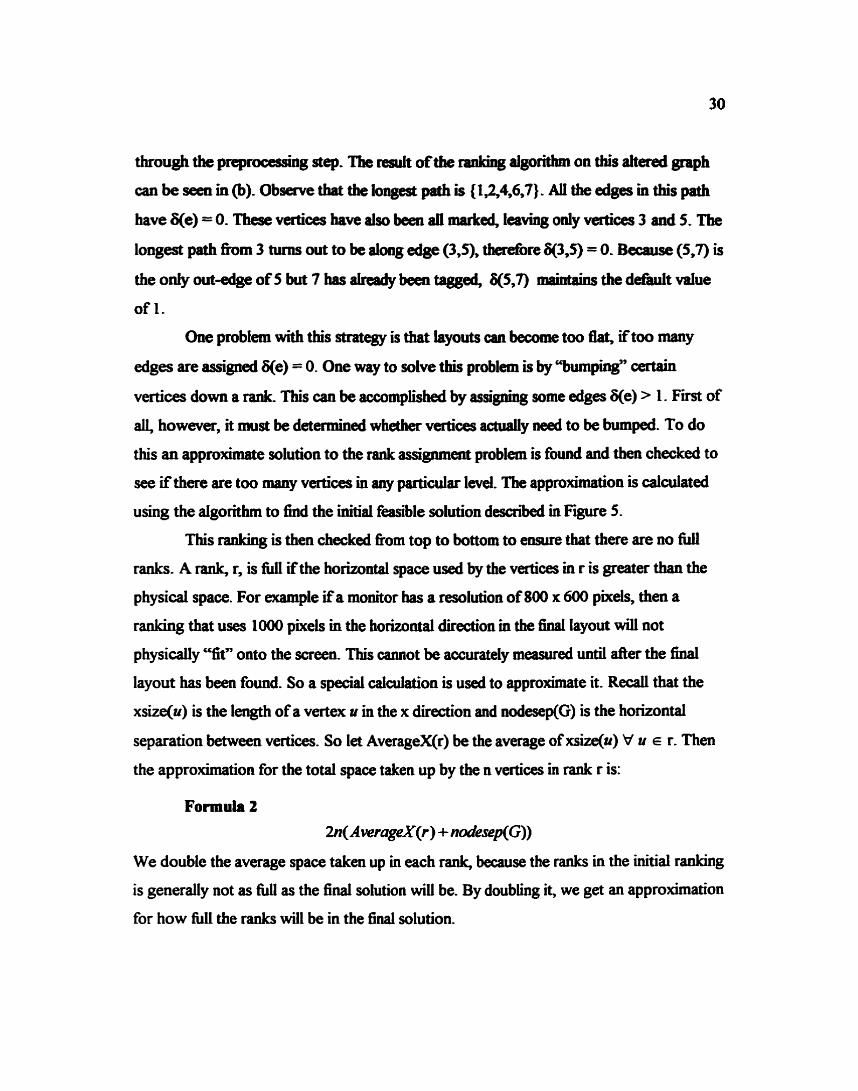
greatest outdegree on the previou rank (r-1) is always
bumped, by assigning its shortest in-edge, e, Re) =
F i i 14
1. initinitrank(); 2. r = RankFullO; 3. while(r!ail) do 4- a - ( r ) ; 5. initinitrank(); 6. r = RankFull.0; 7. end
6(e)+l. tfthe vertex has alnady been bumped once, it is ignored, and the next vertex of
highest outdegree is bumped instead and all approximations are recalculated. Figure 14
shows the pseudo code for this part ofthe algorithm RankFullo the rank first rank
that does not meet the 'W criteria ArraageRank(r) then bumps a vertex fiom the
previous rank and modifies the ranking- A check is done to see ifthe rank is now
acceptable. If it is not, the process is repeated. Figure 15 shows the algorithm.
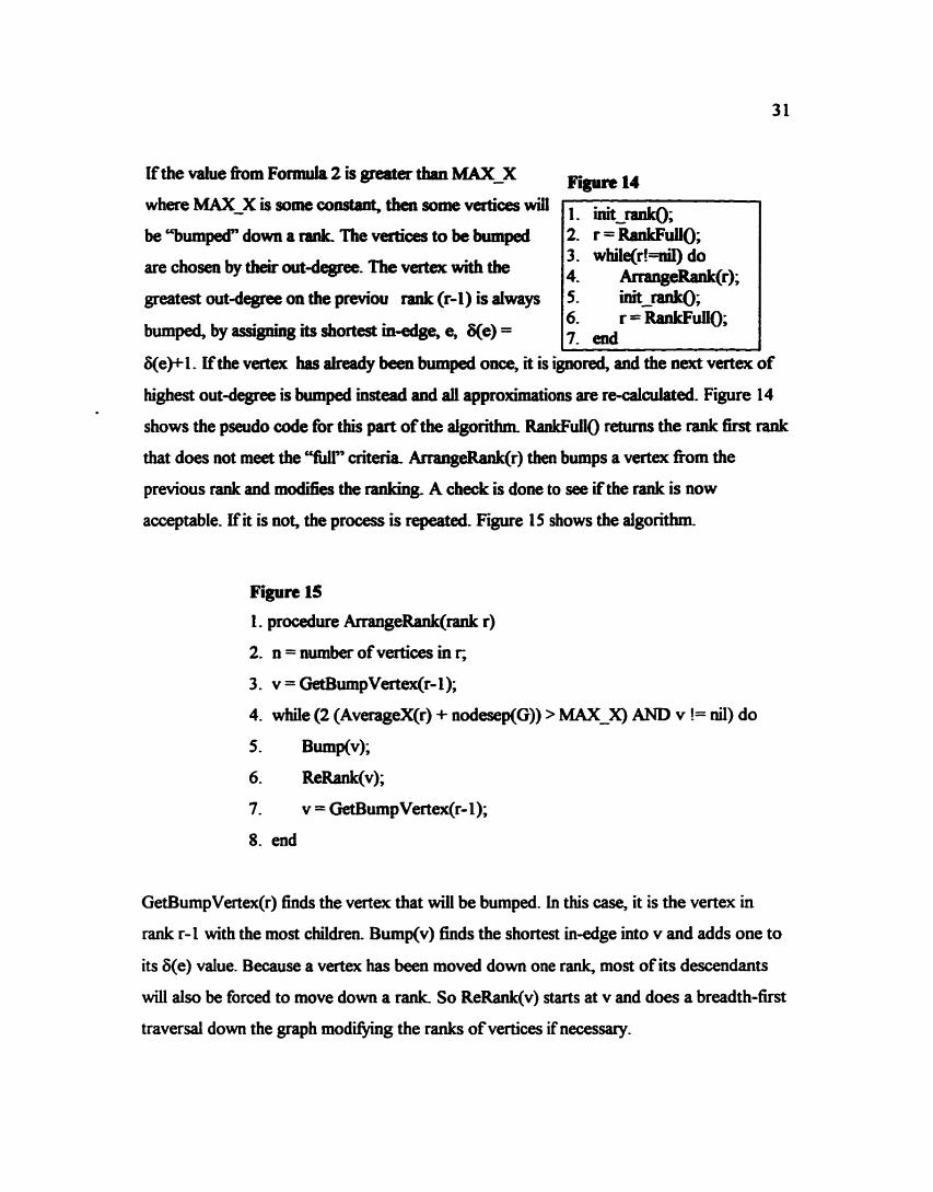
Figure 15
I. procedure ArrangeRank(rank r)
2. n = number of vertices in r,
3. v = GetBumpVertex(r-1);
4. while (2 (AverageX(r) + nodesep(G)) > MAX-X) AND v != oil) do
5. Bump@);
6. ReRaak(v);
7. v = GetBumpVertex(r-1);
8. end
GetBumpVertex(r) finds the vertex that will be bumped. In this case, it is the vertex in
rank r-1 with the most children. Bwnp(v) finds the shortest ingdge into v and adds one to
its 6(e) value. Because a vertex has been moved down one rank, most of its descendants
will also be forced to move down a rank So ReRank(v) starts at v and does a breadth-first
traversal down the graph modifying the ranks of vertices if necessary.
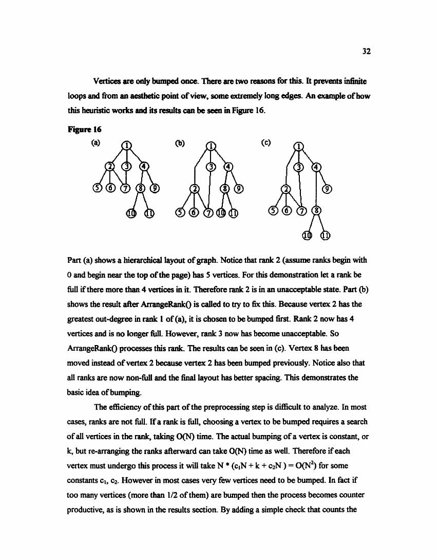
Vertices are only bumped oaa. There are two reasons tbr this. It prevents infmite
loops and tiom an aesthetic point of view, some extremely long edges- An example of how
this heuristic works and its resuits can be seen in Figure 16.
Figure 16
Part (a) shows a hierarchical layout of graph. Notice that rank 2 (assume ranks begin with
0 and begin near the top of the page) has 5 vertices. For this demonstration let a rank be
sin if there more than 4 vertices in it. Therefore rank 2 is in an unacceptable state. Part (b)
shows the result after ArrangeRanko is called to to fix this. Because vertex 2 has the
greatest out-degree in rank 1 of(a), it is chosen to be bumped first. Rank 2 now has 4
vertices and is no longer fU. However, rank 3 now has become unacceptable. So
ArrangeRanko processes this raak. The results can be seen in (c). Vertex 8 has been
moved instead of vertex 2 because vertex 2 has been bumped previously. Notice also that
all ranks are now non-MI and the final layout has better spacing. This demonstratesthe
basic idea of bumping.
The efficiency of this part of the preprocessing step is diiiicult to analyze. In most
cases, ranks are not fUl. Ifa rank is Ml, choosing a vertex to be bumped requires a search
of all vertices in the rank, taking O(N) time. The a d bumping of a vertex is constant, or
but re-arranging the ranks aftenward can take O(N) time as well. Therefore ifeach
vertex must undergo this process it will take N * (clN + k + czN ) = 0(N2) for some
constants cl, cz. However in most cases very few vertices need to be bumped. In fact if
too many vertices (more than 1/2 of them) are bumped then the process becomes counter
productive, as is shown in the results section. By adding a simple check that counts the
number ofbumped vertices, the proass can be stopped at my pticuhr point, K where K
is the maximum number of vertices bumped- In this case, the algorithm becomes K * O(N)
=o(N).
Therefore the entire preprocessing step caa take O(N+M) + O(N) the. Tbis is
much more efficient tban the other stages of the algorithm presented in [GKNV93]. In
fact, the time spent in computing this step is insignificant with nspsd to the rest of the
algorithm. What is interesting however, is that by doing this, the fiaal layout in most cases
is better than those found by usingjust the ideas presented in [GKNV93]. Also, the
preprocessing step makes a huge diffknce in the runniqg time of the algorithm. These
claims will be discussed in chapter 5.
Recall that the Ordering0 procedure in [<iKNV93 J uses heuristics to moday the
ordering of vertices in the ranks, so that the rnunber ofedge ctossings is reduced. One
problem with this solution how- occurs when d&g with flat edges If vertices
w~ected by f h edges are moved around individuatl~~ it is quite possible the edges may
overlap one another, go through a vertex, or point in the opposite direction to other flat
edges. To stop this 60m happening, a p r e - p d g step goes through one rank at a time
looking for vertices that have edges connecting vertices in the same rank These vertices
are then placed side-by-side in the ordering For the purpose of this paper the parent
vertex is placed to the left of the child. This way all Bat edges win point firom left to right.
An important property of vertices connected by flat edges is that their ordering
must be fixed. So any modification of the ordering must rdect this initial ordering. This is
done by merging chains ofvertices comected by flat edges into individual nodes. These
nodes are then moved around as deemed necessary by the transpose and median methods.
Once the ordering has been finalized, they are returned to their original cotlfiguration
This is beneficial because it reduces the number of vertices that the node ordering
heuristics will have to deal with. In cases where there are long chains of vertices
comected by flat edges, huge improvements in efficiency can be seen. This however may
result in a greater number of edge crossings.
Chapter 5-Resub
When compariag the r d t s of two differeat graph drawing algorithms, it is not
enough to say one picture looks better than another. The questions of how and why it is
better must be answered. The m a lies in developing a set of measurable aesthetic
criteria, that can be used to compare the respective layouts. For example in the literature
many algorithms quote the number of edge crossings as a measurable characteristic. Since
many algorithms deal with m g to minimin the number of edge crossings, this
characteristic is very important to their results How these r d t s compare to those of
other existing algorithms is a measure of how well the algorithm worked.
The quality ofthe picture is not the ody important fatwe of the algorithm
Efficiency is always an important measurable quantity. In fict the major problem in
drawing directed hierarchical graphs is the computational time needed to draw large
graphs. In the past ten years much of the work done has been involved in rnodifjhg well
known algorithms so that they work Wer and on graphs with hundreds or thousand of
vertices and edges.
This section analyses the results of using flat edges as a pre-processing step to
Gansner et aL's hierarchical directed graph drawing algorithm called "dot". It will be
shown that with the pre-processing step added to dot (which Eom now on will be referred
to as "flatdag"), pictures of equal or greater quality will be produced in a far more
efficient manner than dot.
This will be done in four sections based on the analysis techniques discussed in
[JOHNS96]. The first will define the basic attributes ofa graph, and how they will be
measured quantitatively. The second will compare the quality of the drawings output fkom
flatdag and dot with some originally published drawings from Sugiyama et d. 's paper on
drawing hierarchical directed graphs. The third section will look at the quality of drawings
of flatdag compared with those specifically from dot. The final section will then look at a
comparison of the efficiency of these two algorithms.
It is not an easy problem to objectively measure the aesthetics of a graph
However, since tbe final goal of flat@ is to produce layouts that are easily readable, bsn
cornparabie height and width, a d are computationally amactive, the fillowing measurable
characteristic will beused to comparethelayoutsofflatdagwithotherdgaithms.
The first measurable attriiute ofany layout is the number of ranks or levels in the
hierarchy and how it compares with its width. Many graph drawing algorithms produce
pictures with a disproportionate number of levels compared to the width. Tbis results in
two potential problems. Because human be- perceive pictures as whole before they
perceive specifics [GRAY911 and [GEST47l, a good layout should have an even
distriiution ofvertices in both the horizontal and vertical direction Having vertices placed
in such a manner provides even spacing between nodes and dormity throughout the
drawing. The second and more important problem, is that having more levels results in
having a greater number of dummy or virtual nodes added to the graph, Most hierarchical
drawing algorithms for directed graphs insert these nodes into their layouts in order to
produce better pictures. However, this enlarges the size of the graph. Therefore reducing
the number of virtual nodes will be beneficial for the efficiency of the algorithm.
The ratio of width to height could be measured in terms of the maximum x and
maximum y coordinate that occur in the final layout. Unfortunately this is not the best way
of doing it. Note that these values can differ greatly by the value ofwhat constants are
used to express the distance between ranks, the minimum distance between vertices in the
same rank, not to mention the size of each vertex. So for this paper, the ratio will be
measured by the total number of ranks (height), and the maximum number ofvertices in
any rank in the final layout (width). It should be noted however, that in this paper the
distance between two consecutive ranks is approximately 2.5 times the minimum distance
between the center of vertices in the same rank. Because a "good" ratio between width
and height of a drawing in principle is 1: 1, for dot and flatdag an equivalently good ratio is
2.5: 1.
One way to evaluate how much the number ofvirhltl nodes adds or detracts &om
a layout ofgraph is by m d g the sum of the total edge length Since long edges
reduce the readability ofa layout, it is important to have this mrmrmzed * * . - R e d l that fir the
purposes ofthis paper the length of an edge (UJ) is not the Euclidean distance, but
defied as the positive dBmmce between rank(u) and rank(v).
Another measurable a - i e that deals with the readability of a layout is the
number of edge crossings. Because tbis tends to be a very important meamable quantity it
will be used in this section as a measuring stick to compare these results with those of
&sting algorithms.
So for measuring the aesthetics ofa layout these three qU8iifies will be measured:
the relationship between the width and the height
the sum of the total edge length
the number of edge aossings in the graph
They will be used to compare and contrast the results of the algorithm proposed in this
paper and those of previously published algorithms.
5.3 Objective M-sums - Effciency
Measuring something subjectively, like the aesthetic qualities of a drawing, is not
any easy task, but the opposite is true for something objective. The efficiency of an
algorithm can be determined in a number of ways. The first is to measure how many
seconds it takes to complete. The second is to monitor how many iterations are undergone
before the algorithm is complete. Because the implementations of flatdag and dot are not
necessarily optimized, the number of iterations undergone may be more significant than
the actual speed of the algorithm It should be noted however, that the only differences in
the implementations is the pre-processing step that is used in flatdag. Thus the difference
in efficiency is a reflection of what the pre-processing step does to the initial
characteristics of the graph and not the different implementations.
Another mdhod of maiming the efticiency is by following how the graph changes
as it goes through each step. For exampie Gaasner et d. noted that the positioning step
uses a disproportiouate amount of time to complete compared with the otha stages. This
is caused by the increased size of the augmented graph used in this stage. By knowing the
number ofedges and vertices that are used in the positioning step, it is easy to see changes
as a d t of which dgorithm is used.
Thus the Sciency oftlatdag and dot win be measured in three ways: actual time
taken to complete, number of iterations used in each step, and the size ofthe graph that is
used in the positioning step.
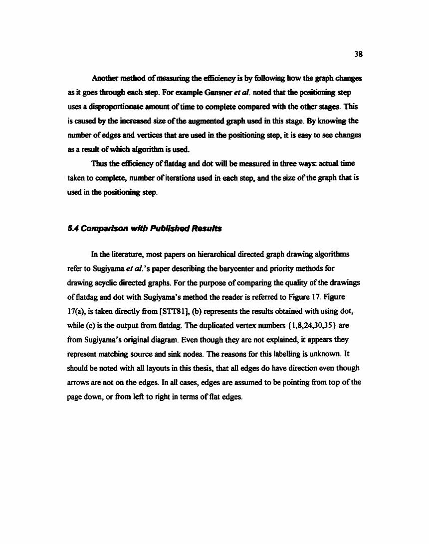
5.4 Compan'son with Published Resuits
In the literatwe, most papers on hierarchical directed graph drawing algorithms
refer to Sugiyama et al.3 paper descniig the barycenter and priority methods for
drawing acyclic directed graphs. For the purpose of comparing the quality of the drawings
of flatdag and dot with Sugiyama's method the reader is referred to F i e 17. Figure
17(a), is taken directly fiom [STT81], (b) represents the results obtained with using dot,
while (c) is the output £kom flatdag. The duplicated vertex numbers (1,8,24,30,35) are
from Sugiyama's original diagram. Even though they are not explained, it appears they
represent matching source and sink nodes. The reasons for this labelling is unknown It
should be noted with all layouts in this thesis, that ell edges do have direction even though
arrows are not on the edges. In all cases, edges are assumed to be pointing from top of the
page down, or fiom left to right in terms of flat edges.
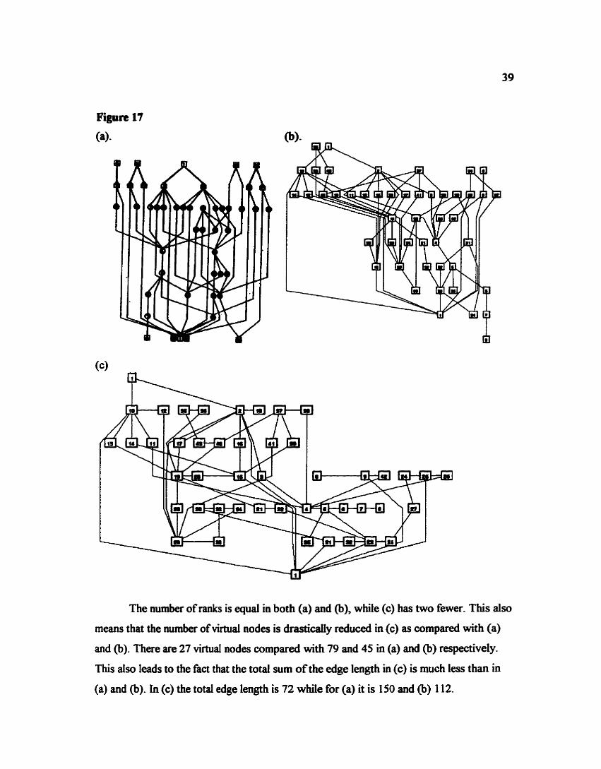
The number of ranks is equal in both (a) and (b), whife (c) has two fewer. This also
means that the number of virtual nodes is drastically reduced in (c) as compared with (a)
and (b). There are 27 virtual nodes compared with 79 and 45 in (a) and @) respectively.
This also leads to the fact that the total sum of the edge length in (c) is much less than in
(a) and (b). In (c) the total edge length is 72 while for (a) it is 150 and (b) 1 12.
Furthermore picture (c) bas f i e r edge crossings thn both (a) and (b), 44 compared with
61 and 67 nspeaiveiy. Also, try to determine incoming edges to vertex 29. We tbink this
easier to do in Figure 17(c).
The last measured criterion is the reIatioaship between the maximum number of
nodes in a rank with respect to the number ofmks. In this case, all thne layouts are very
similar. (a) has a 2.3: 1 ratio while (b) and (c) bave a 2.2: 1 and 3: 1 ratio. On obsenmtioa
however, Figure l(c) does have a more uniform distribution of vertices per rank compared
with (a) and (b).
Therefore according to the measured aesthetic criteria, the layout produced by
flatdag is superior to those produced by the other two algorithms because it has less total
edge length, fewer edge crossings and a better distribution of vertices than (a) and @).
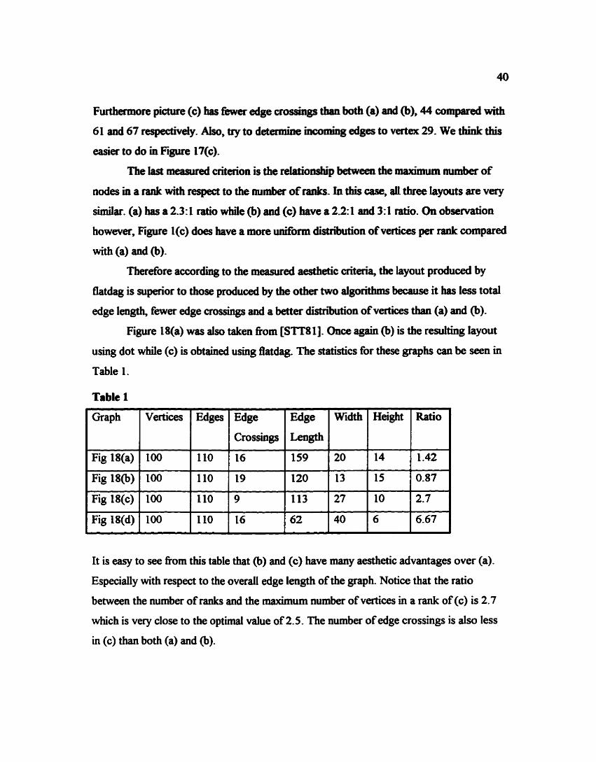
Figure 18(a) was also taken fiom [STI8 I]. Once again @) is the resulting layout
using dot while (c) is obtained using Batdag. The statistics for these graphs can be seen in
Table 1.
Table 1
It is easy to see from this table that @) and (c) have many aesthetic advantages over (a).
Especially with respect to the overall edge length of the graph. Notice that the ratio
between the number of ranks and the maximum number of vertices in a rank of (c) is 2.7
which is very close to the optimal value of 2.5. The number of edge crossings is also less
in (c) than both (a) and (b).
Height
14
15
10
6
Width
20
13
27
40
Graph
Fig 18(a)
Fig 18(b)
Fig 18(c)
Fig 18(d)
Ratio
1 -42
0.87
2.7
6.67
Vertices
100
100
100
100
Edges
110
110
110
110
Edge
Crossings
16
19
9
16
Edge
Length
159
120
113
62

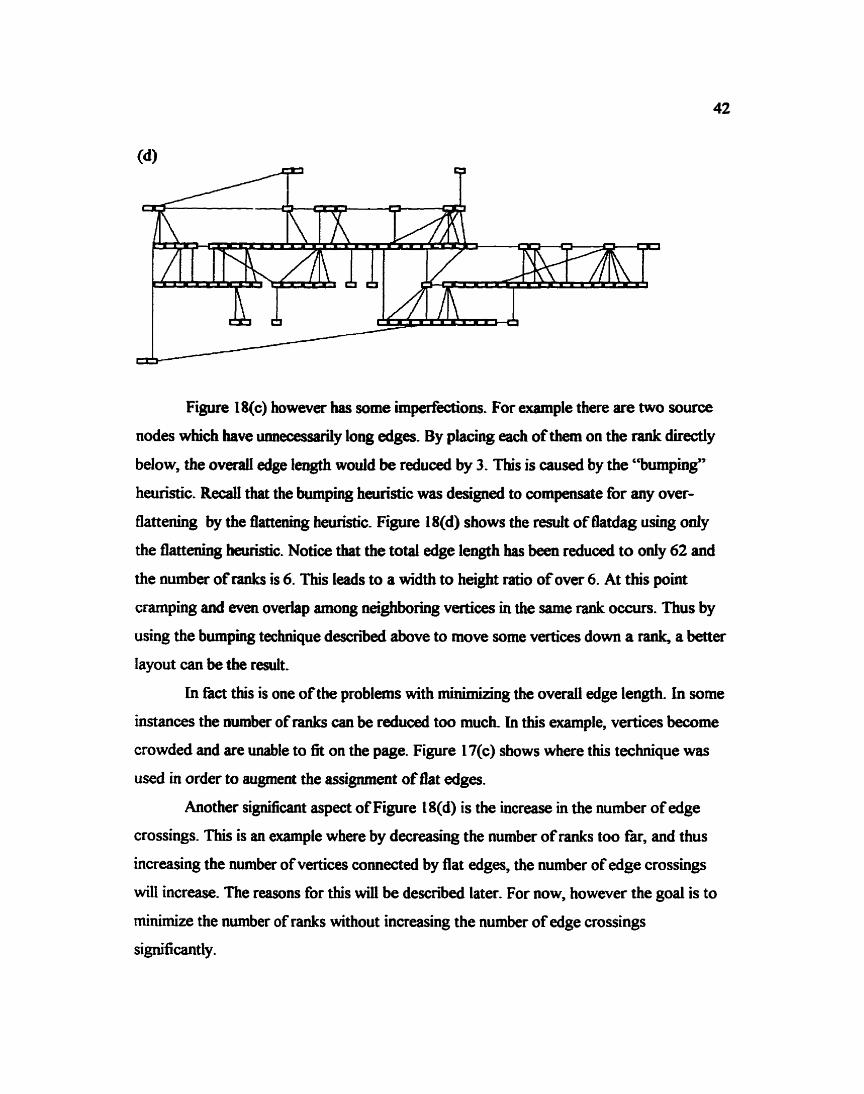
Figure 18(c) however has some imperfections. For example there are two source
nodes which have mecessarily long edges. By placing each ofthem on the rank directly
below, the oved edge length would be reduced by 3. This is caused by the '%urnping"
heuristic. Recall that the bumping heuristic was designed to compensate for any over-
flattening by the flattening heuneunsticC Figure 18(d) shows the result of tlatdag using only
the flattening heuristic. Notia that the total edge length has been reduced to only 62 and
the number of ranks is 6. This leads to a width to height ratio of over 6. At this point
cramping and even overlap among neighboring vertices in the same tank occurs. Thus by
using the bumping technique d e s c n i above to move some vertices down a ranlc, a better
layout can be the result.
In fact this is one of the problems with minimiziog the overall edge length. In some
instances the number of ranks can be reduced too much. In this example, vertices become
crowded and are unable to fit on the page. Figure 17(c) shows where this technique was
used in order to augment the assignment of flat edges.
Another significant aspect of Figure 18(d) is the increase in the number of edge
crossings. This is an example where by decreasing the number ofranks too far, and thus
increasing the number of vertices co~ected by flat edges, the number of edge crossings
will increase. The reasons for this will be d e s c n i later. For now, however the goal is to
minimize the number of ranks without increasing the number of edge crossings
significantly.
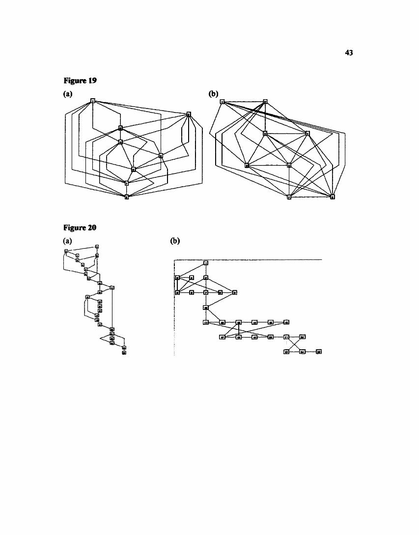
Figure 20
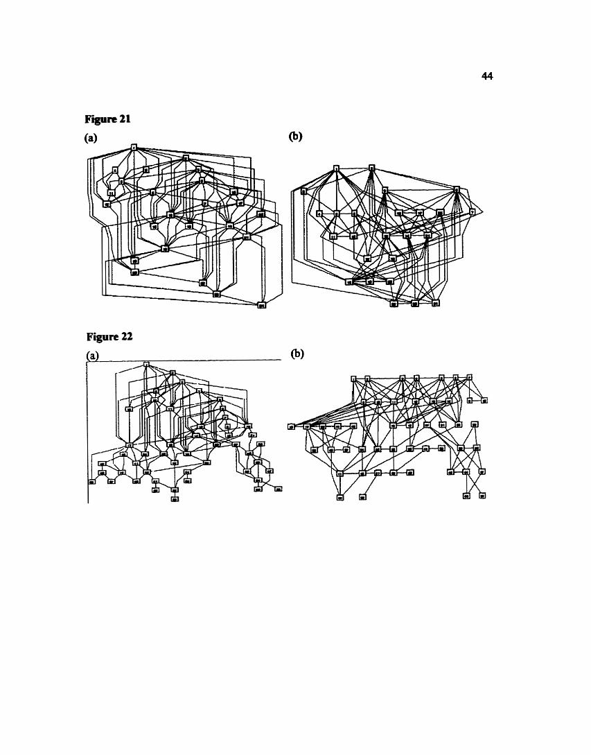
Figure 22
Figure 24
(a)
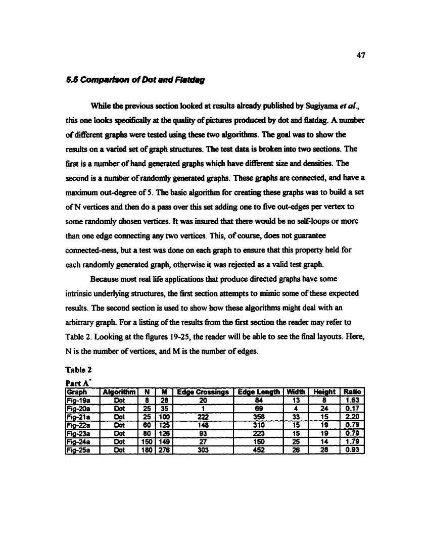
5.5 Compatkon of Dot and F h t d '
While the previous d o n looked at results elready published by Sugiyama et d.,
this one looks spedcally at the quality of pictures produced by dot and flatdag A number
of different graphs were tested using these two algorithms. The goal was to show the
results on a varied set of graph structures- The test data is broken into two sections. The
first is a number of band generated gnphs which have di&rrnt size and densities. The
second is a number ofrandomly generated graphs. These grapbs ace connected, and have a
maximum outdegree of 5. The basic algorithm for creating these graphs was to build a set
of N vertices and then do a paps over this set adding one to five out-edges per vertex to
some randomly chosen vertices. It was insured that there would be no self-loops or more
than one edge c o d g any two vertices. This, of course, does not guarantee
connected-new, but a test was done on each graph to ensure that this property held for
each randomly generated graph, otherwise it was rejected as a valid test graph-
Because most real life applications that produce directed graphs have some
intrinsic underlying structures, the first section attempts to mimic some of these expected
results. The second section is used to show how these algorithms might deal with an
arbitmy graph. For a listing of the r d t s fiom the first section the reader may refer to
Table 2. Looking at the figures 19-25, the reader will be able to see the final layouts. Here,
N is the number ofvertices, and M is the number of edges.
Table 2
Part A'
Fig-23a 93 223 15 19 0-79 Fig-24a Dot 150 149 27 150 25 14 ,. 1.79, Fig-25a Dot 180 276 303 452 26 28 0.93 .
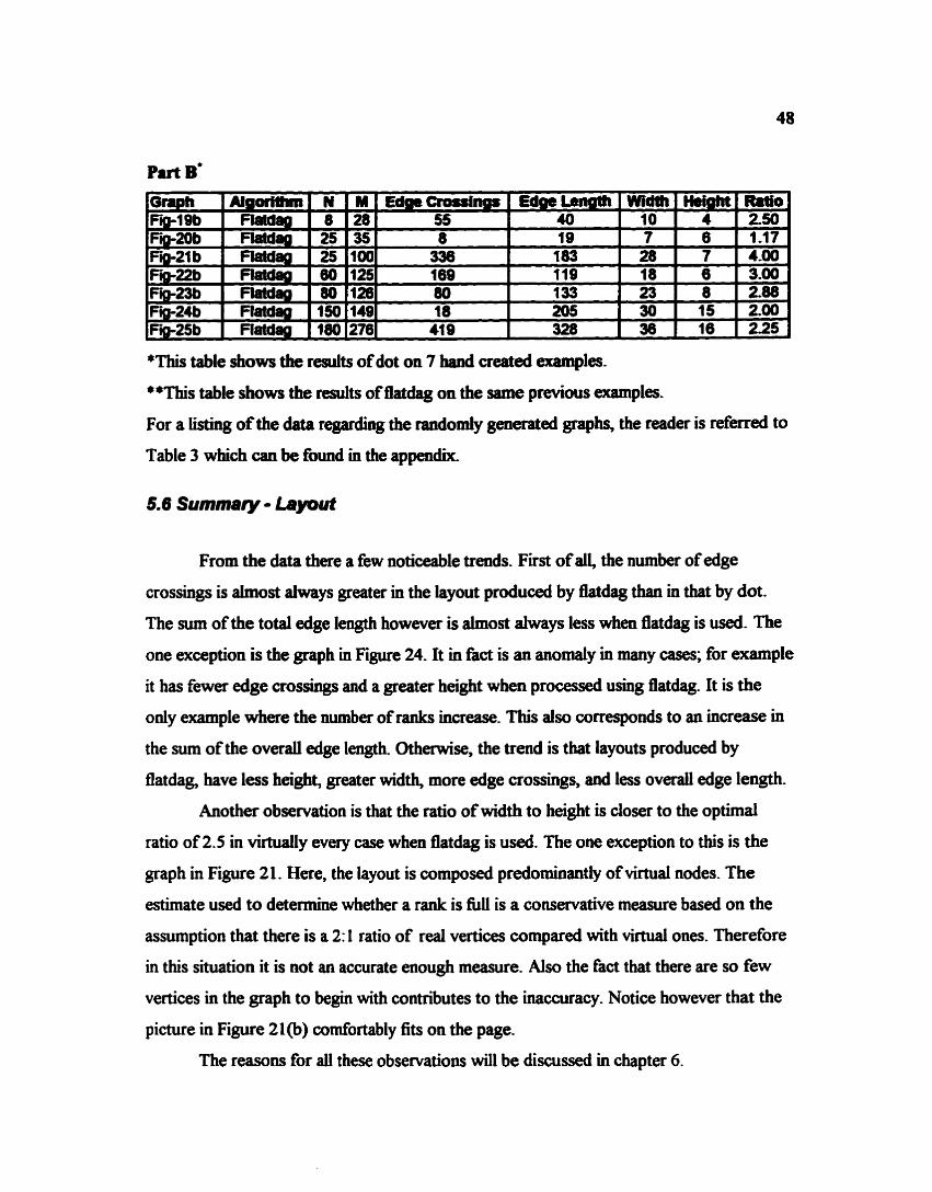
P u t B'
*This table shows the results of dot on 7 hand created examples.
**This table shows the results of flatdag on the same previous examples.
For a listing of the data regarding the randomly generated graphs, the reader is r e f d to
Table 3 which can be found in the appendix,
5.6 Surnmaty - Layout
From the data there a few noticeable trends. First o f 4 the number of edge
crossings is almost always greater in the layout produced by Batdag than in that by dot.
The sum of the total edge length however is almost always less when flatdag is used. The
one exception is the graph in Figure 24. It in fact is an anomaly in many cases; for example
it has fewer edge crossings and a greater height when processed using flatdag. It is the
only example where the number ofranks increase. This also corresponds to an increase in
the sum of the overall edge length Otherwise, the trend is that layouts produced by
flatdag, have less height, greater width, more edge crossings, and less overall edge length-
Another observation is that the ratio of width to height is closer to the optimal
ratio of 2.5 in virtually every case when flatdag is used. The one exception to this is the
graph in Figure 21. Here, the layout is composed predominantly of virtual nodes. The
estimate used to determine whether a rank is fU is a conservative measure based on the
assumption that there is a 2: 1 ratio of real vertices compared with virtual ones. Therefore
in this situation it is not an accurate enough measure. Also the fact that there are so few
vertices in the graph to begin with contributes to the inaccuracy. Notice however that the
picture in Figure 21(b) comfortably fits on the page.
The reasons for all these observations will be discussed in chapter 6.
This section looks a the di&rence in the oved speed of the two algorithm.
Table 4 shows the results ofthe haad created examples used above while Table 5 shows
the results of the algorithms on the 27 randomly generated graphs. For ease of reading,
both of these tables appear in the appendix
The data d e s c r i i 3 dierent ways of looking at efliciency- The first is how fm in
terms of seconds each stage of the algorithm runs and how fist the algorithm is overall.
Secondly, it looks at how the size of the graph changes as it goes through each of the
three phases of the algorithms. The third is the number of iterations that the positioning
step takes before it comes to completion. All three of these parts express the efficiency of
these algorithms fiom a slightly different angIe which is important in determining why one
is more efficient than t&e other,
5.8 ObsewaUons - Efficiency
In every case, with the exception of the graph fiom Figure 24, flatdag was much
faster than dot. The ranking steps were approximately equal, but the ordering and position
steps were both much faster in flatdag. Also, the size of the awdliary graph used in the
positioning step is much greater when nm using dot.
The Rank stage which includes the pre-processing step for flatdag took almost the
same amount of time- As the graphs became larger the difference in time became less. The
opposite is true for both the ordering and positioning steps. In all cases, with the exception
of the graph in Figure 24, ordering and positioning steps were much faster. As the graphs
became larger the difference between the speed ofdot and flatdag also becomes greater.
In fact, in some of the experiments dot takes 10 hours to complete. In comparison, flatdag
takes only 6 1/2 minutes.
The reasons for these observations will be answered in the following chapter.
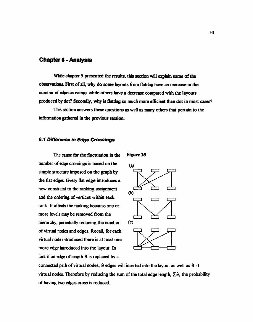
Chapter 6 - Analysb
While chapter 5 presented the r d t s , this section wilI explain some of the
observati~ns~ First of a& why do some layouts from Mdag have an increase in the
number of edge crossings while others have a decrease compared with the layouts
produced by dot? Secondly, why is Bat* s9 much more acient than dot in most cases?
This section answers these questions as wen as many others that pertain to the
information gathered in the previous section
6.1 Difiiellence in Edge Cmssings
The cause for the fluctuation in the
number of edge crossi~~gs is based on the
simple structure imposed on the graph by
the flat edges. Every flat edge introduces a
new constraint to the ranking assignment
and the ordering of vertices within each
rank. It affects the ranking because one or
more levels may be removed fiom the
hierarchy, potentially reducing the number
of virtual nodes and edges. Recall, for each
virtual node introduced there is at least one
more edge introduced into the layout. In
fact if an edge of length 9 is replaced by a
Figure 25
connected path of virtual nodes, 9 edges will inserted into the layout as well as 9 -1
virtual nodes. Therefore by reducing the sum of the total edge length, Z9, the probability
of having two edges cross is reduced.
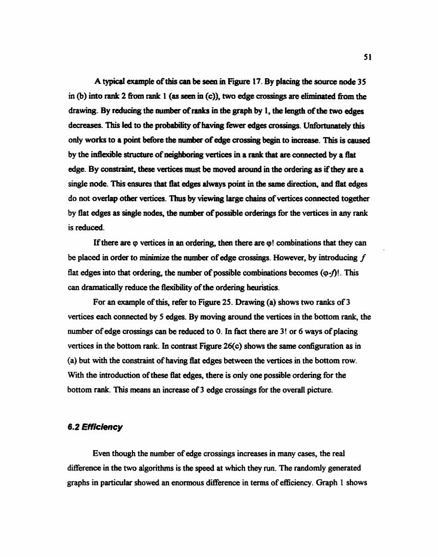
A typid example of this can be seen in Figure 17. By placing the source node 35
in (b) into rank 2 &om rank 1 (as seen in (c)), two edge crossings are ehinated from the
drawing- By reducing the mmber ofranks in the graph by I, the length of the two edges
decreases. This led to the probability of k i n g fewer edges crossiags. Unfortunately this
only works to a point Wore the number of edge crossing begin to increase- This is caused
by the inflexible structure of neighboring vertices in a rank that are connected by a fht
edge. By constrainf these vertices must be moved around in the ordering as if they are a
single node. This ensures tbat flat edges always point in the same direction, and flat edges
do not overlap other vertices. Thus by v i d g large chsins ofvefti~e~ ~ ~ ~ e c t e d together
by flat edges as SingIe nodes, the number of possible orderings for the vertices in any rank
is reduced.
Ifthere are cp vertices in an ordering, then there are cp! combinations that they can
be placed in order to minimize the number of edge crossings- However, by introducing f
flat edges into that ordering the number of possible combinations becomes (q-fi!. This
can dramatically reduce the flexibility of the ordering heuristics.
For an example of this, refer to Figure 25. Drawing (a) shows two ranks of 3
vertices each ~ ~ ~ e c t e d by 5 edges. By moving around the vertices in the bottom rank, the
number of edge crossings can be reduced to 0. In fact there are 3! or 6 ways of placing
vertices in the bottom rank. In contrast Figure 26(c) shows the same configuration as in
(a) but with the constraint of having flat edges between the vertices in the bottom row.
With the introduction of these flat edges, there is only one possible o r d e ~ g for the
bottom rank. This means an increase of3 edge crossings for the overall picture.
Even though the number of edge crossings increases in many cases, the real
difference in the two algorithms is the speed at which they run. The randomly generated
graphs in particular showed an enormous difference in term of efficiency. Graph 1 shows
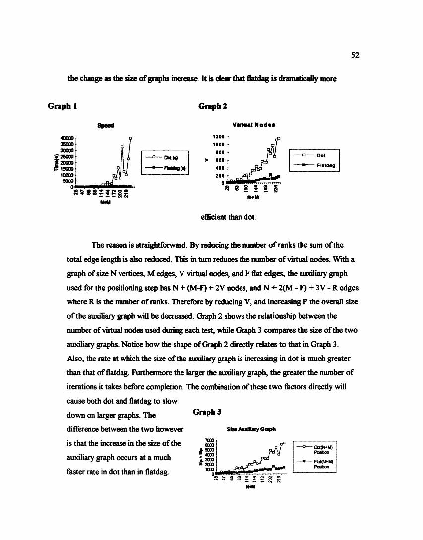
the change as the size of graphs increase- It is clear that flat- is dramatidy more
Virtual Nodes
1200 1 ff
efficient than dot.
The reason is straightfornard. By reducing the number of ranks the sum of the
total edge length is also reduced. This in turn reduces the number of virtual nodes. Wnh a
graph of size N vertices, M edges, V virtual nodes, and F flat edges, the auxiliary graph
used for the positioning step has N + (M-F) + 2V nodes, and N + 2(M - F) + 3V - R edges
where R is the number of ranks. Therefore by reducing V, and increasing F the overall size
of the auxiliary graph win be decreased. Graph 2 shows the relationship between the
number of virtual nodes used during each test, while Graph 3 compares the size of the two
auxiliary graphs. Notice how the shape ofGraph 2 directly relates to that in Graph 3 .
Also, the rate at which the size of the d a r y graph is increasing in dot is much greater
than that offlatdag. Furthemre the larger the auxiliary graph, the greater the number of
iterations it takes before completion. The combination of these two factors directly will
cause both dot and flatdag to slow
down on larger graphs. The Graph 3
Merence between the two however s i i ~uxiwyonph
is that the increase in the size of the
auxiliary graph occurs at a much
faster rate in dot than in flatdag.
M a
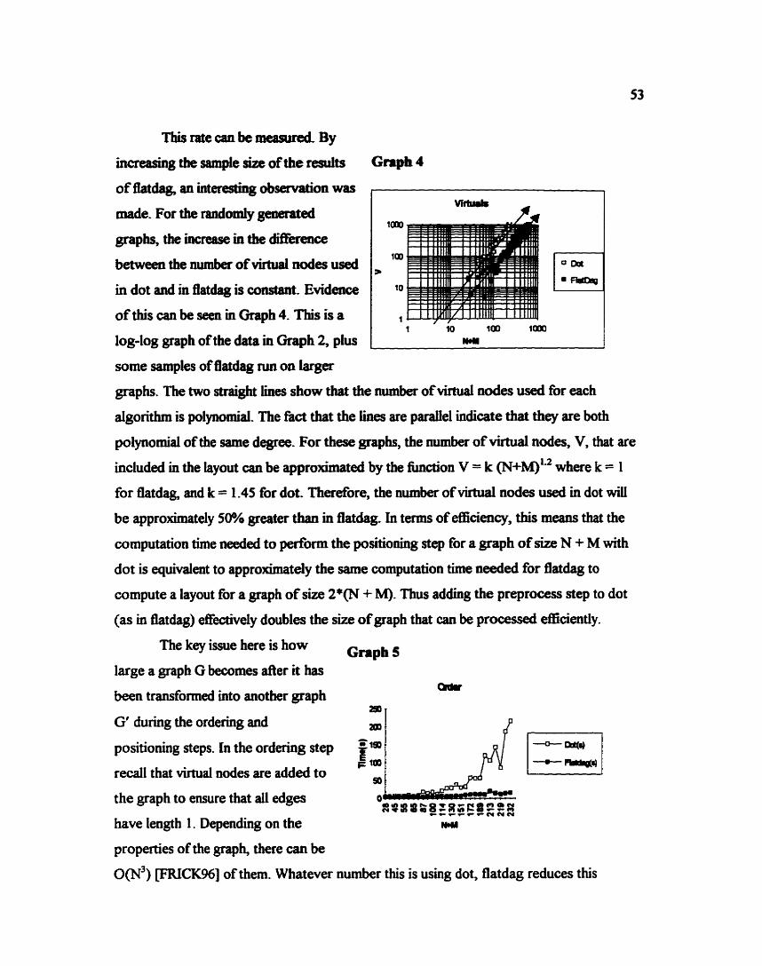
Tbis rate can be mYurrd By
increasing the sample size of the results Gmph 4
of flatdag, an heresting &sendon was
made. For the randomly generated
graphs, the increase in the difference
between the number of virtual nodes used
in dot and in flatdag is constant. Evidence
of this can be seen in Graph 4. This is a
log-log graph of the data in Graph 2, plus
some samples of flatdag NO on larger
1 - lo 100 two ma
graphs. The two straight lines show that the number ofvirtual nodes used for each
algorithm is polynomial. The fhct that the lines are parallel indicate that they are both
polynomial of the same degree- For these graphs, the number of virtual nodes, V, that are
included in the layout can be approximated by the hction V = k (N+M)'~ where k = 1
for flatdag, and k = 1.45 for dot. Therefore, the number of virtual nodes used in dot will
be approximately 50% greater than in flatdag. In terms of efficiency, this means that the
computation time needed to perform the positioning step for a graph of size N + M with
dot is equivalent to approximately the same computation time needed for flatdag to
compute a layout for a graph of size 2*(N + M). Thus adding the preprocess step to dot
(as in flatdag) effectively doubles the size of graph that can be processed efficiently.
The key issue here is how Gnph large a graph G becomes after it has
been transformed into another graph
G' during the ordering and
positioning steps. In the ordering step fls
recall that virtual nodes are added to F $90
50
the graph to ensure that all edges o SoaosgffflfgEES - -
have length 1. Depending on the WM
properties of the graph, there can be
0(N3) w C K 9 6 ] of them. Whatever number this is using dot, flatdag reduces this
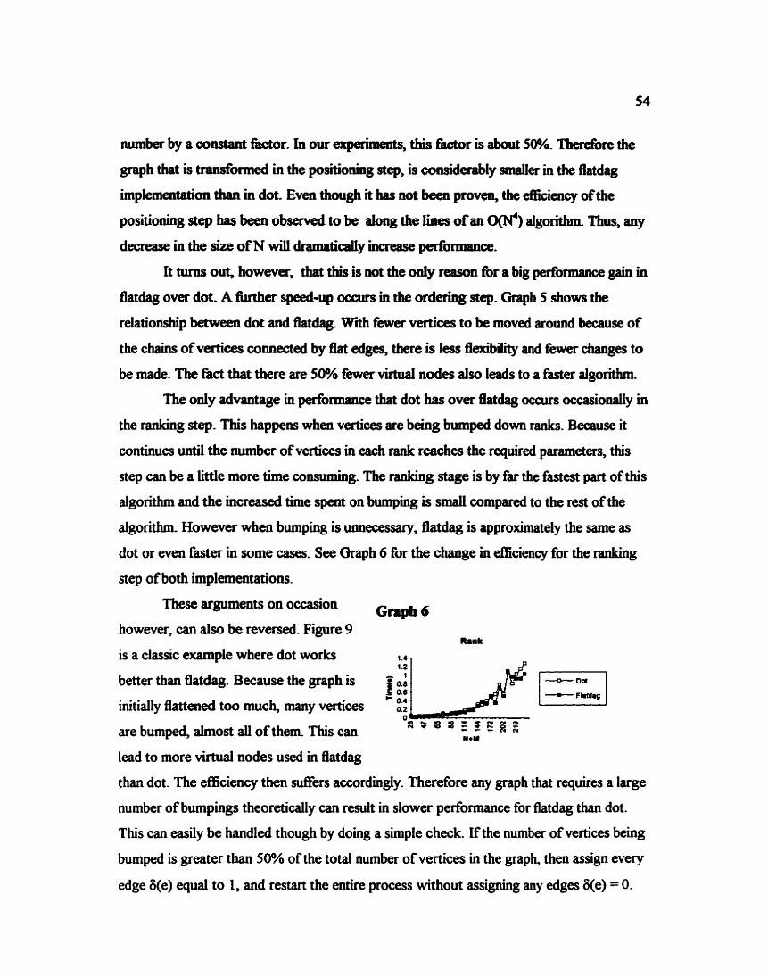
number by a constant fkctor- In our eqxhmts7 this -or is about 5W. Therefore the
graph that is transformed in the positioning step, is considerably smaller in the flatdag
implementation than in dot- Even though it has not been proven, the &cimcy of the
positioning step has been obsnved to be dong the lines of an O(N*) algorithm Thus, any
decrease in the size of N will dramaticaUy increase pedior~~~ce.
It turns out, however, that this is not the only reason for a big performance gain in
flatdag over dot. A fiuther speed-up occurs in the ordering step. Graph 5 shows the
relationship between dot and flatdag. Wnh fiwer vertices to be moved around because of
the chains of vertices ~ ~ ~ e c t e d by flat edges, there is less flexi%*ty and fewer changes to
be made. The fact that there are 50% fewer virtual nodes also leds to a f a e r algorithm.
The ody advantage in performance that dot has over flatdag occurs occasionally in
the &g step. This happens when vertices are being bumped down ranks. Because it
continues until the number of vertices in each rank reaches the required parameters, this
step can be a little more time consuming. The ranking stage is by fbr the fastest part of this
algorithm and the increased time spent on bumping is small compared to the rest of the
algorithm. However when bumping is u~ecessary, flatdag is approxhately the same as
dot or even faster in some cases. See Graph 6 for the chaage in aciency for the ranking
step of both implementations.
These arguments on occasion Graph 6 however, can also be reversed. Figure 9
Rank
is a classic example where dot works 1.1 I
better than flatdag. Because the graph is
init idly flattened too much, many vertices
are bumped, almost all of them. This can
lead to more virtual nodes used in flatdag
than dot. The efficiency then suffers accordiiy. Therefore any graph that requires a large
number of bumpings theoretically can result in slower performance for flatdag than dot.
This can easily be handed though by doing a simple check. If the number of vertices being
bumped is greater than 50% of the total number of vertices in the graph, then assign every
edge 6(e) equal to 1, and restart the entire process without assigning any edges 6(e) = 0.
Then a layout tiom mdag will be w difZkmt than that of dot in many cases. Of course
the efficiency will d e r , but beause the pre-process@ step takes a very s d amount of
time compared with the rest ofthe algorithm, this is aaeptabIe.
Decreasing the number of ranks in any hierarchical layout, is somewhat precarious
as seen in Figure 18(c). Thus, bumping is necessaq in producing acceptable layouts.
However, this is ody worthwhile when bumping only a small subset of vertices in the
graph Figure 24 is a perfect example ofa graph where too much bumping has occurred.
Here, many vertices have been bumped. The result is a layout that is worse than the one
produced by dot. It also has more ranks, more vimral nodes and a corresponding increase
in the sum of the overall edge length This process works best when only a small subset of
vertices need to be bumped. Graphs that have an ideal hierarchical structure where the
width is much greater than height are not n d y going to be well drawn using flatdag.
The flattening part ofthe preprocess will reduce the number ofranks too much The
bumping part of the preprocess tries to fix this, but is not a good heuristic for wholesale
changes. An example where bumping works reasonably well is Figure 18(c). Bumping
only a few vertices results in a good layout. In this instance 56 vertices were bumped. As
mentioned before however this layout does have imperfectom. It turns out that when
more than SO?? of the vertices are bumped the resulting picture is better when dot is used.
This can be easily be incorporated into flatdag by doing a simple check as mentioned
earlier. To demonstrate how well the bumping heuristic worked, this check was not
incorporated into the implementation of flatdag that produced all the layouts seen in this
paper. Therefore, the bumping part of the preprocessing step is sufficient only when small
changes need to be made to the results of the flattening step. Otherwise better methods
need to be developed to counter act the results of the initial preprocessing step.
Chapter 7 - Conclusions
Flatdag in most cases produces Iayouts that are equal to, if not better than, those
of dot. In all of these cases, the speed offlatdag is fhr superior to that of dot. Because the
speed ofthese two algorithms is determined predominantly by the positioning step, the
number ofvirtual nodes inserted into the graph must be kept to a minimum without
jeopardizing the o v d quality of the picture. In instances where the height exceeds the
width by a large margin in a layout where no flat edges are used, flatdag produces very
good results. Howmr, when the width exceeds the height in the same situation flatdag
does not produce results as good as dot This can be remedied by reverting to dot.
Flatdag produces equal or better layouts at a much faster speed. It has also opened
a few doors for mom research. The assignment of flat edges in this paper is based on a
depth first approach. Preliminary results however show that a breadth-first approach may
be better. For instance, by first calculating the longest path for each edge in the graph,
then doing a breadth-first traversal starting at the source nodes, there is potential for
assigning flat edges in a more intelligent way. Especially if there are more than two edges
which have the same value. Perhaps by allowing some sort oflook-ahead mechanism, to
deduce the immediate surrounding structure of the graph, assignment can be more
intelligent.
Another area that can be looked at is the bumping aspect. The heuristic used in this
paper, is too simple and produces poor results. It was originally designed to counter-act
the possibility that too many edges are assigned a 6(e) = 0. However, it has tumed out to
be practical in only some instances. Observations of the graphs produced by flatdag
without bumping give rise to the possibility that in all cases flatdag, at its worst, could
produce the same result as dot, i.e. no edges are initially assigned 6(e) = 0. This, of course,
is a continuation of how to decide which edges, ifany, should be modified.
This also may lead to help for drawing graphs with excessive width compared to
height. In some examples graphs are so wide compared to their height, that dot does not

produce acaqmhle results eithereithez Adding bumpmg to dot may also be a way of producing
better layouts ahhaugh the layout will take more time to producece
This brings us to the positioning part ofthe algorithm Because the structure ofthe
t r a a s f o d graph is much more constrained than in the ranldag step, there may be ways
of developing short cuts to compute the solution to the hear programming probkm
Thexe also may be other approaches to solving this ptobIem that can use the properties of
the arociliary graph to produce more efficietlf results-
This however, is beyond the scope of this paper and it is presented hen as a
potential topic for firtun w o k The god ofthis paper was to push forward the horizons of
the problem of drawing directed graphs. Ho-y, it has aocomplished this goal.
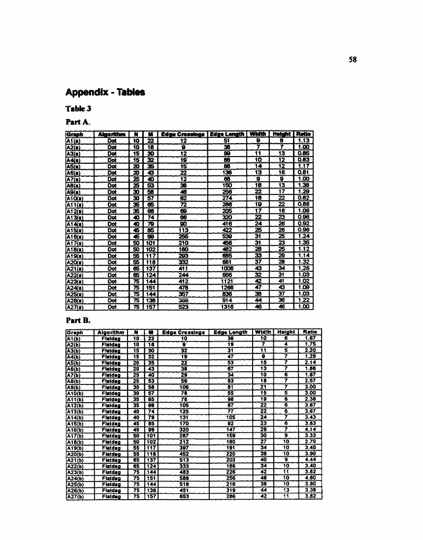
Appendix - Tables
Table 3
P u t A*
Part B.
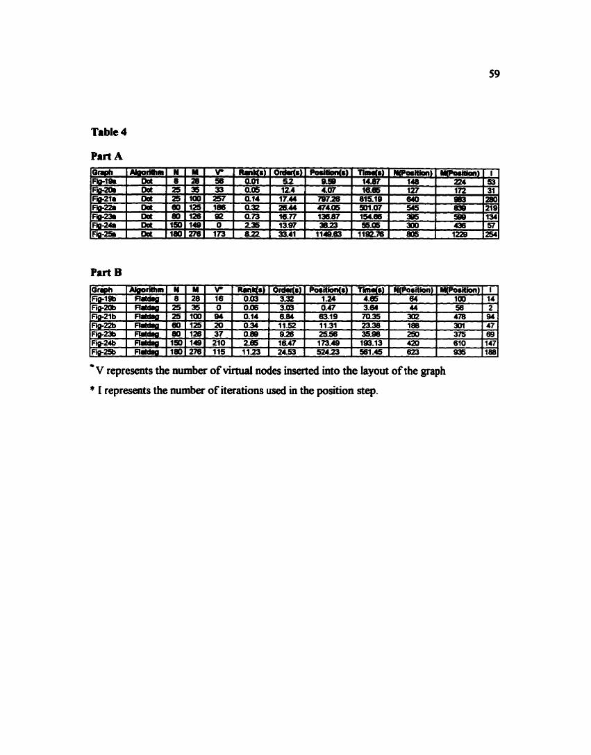
Table 4
Put A
V represents the number of virtuat nodes inserted into the layout of the graph
* 1 represents the number of iterations used in the position step.
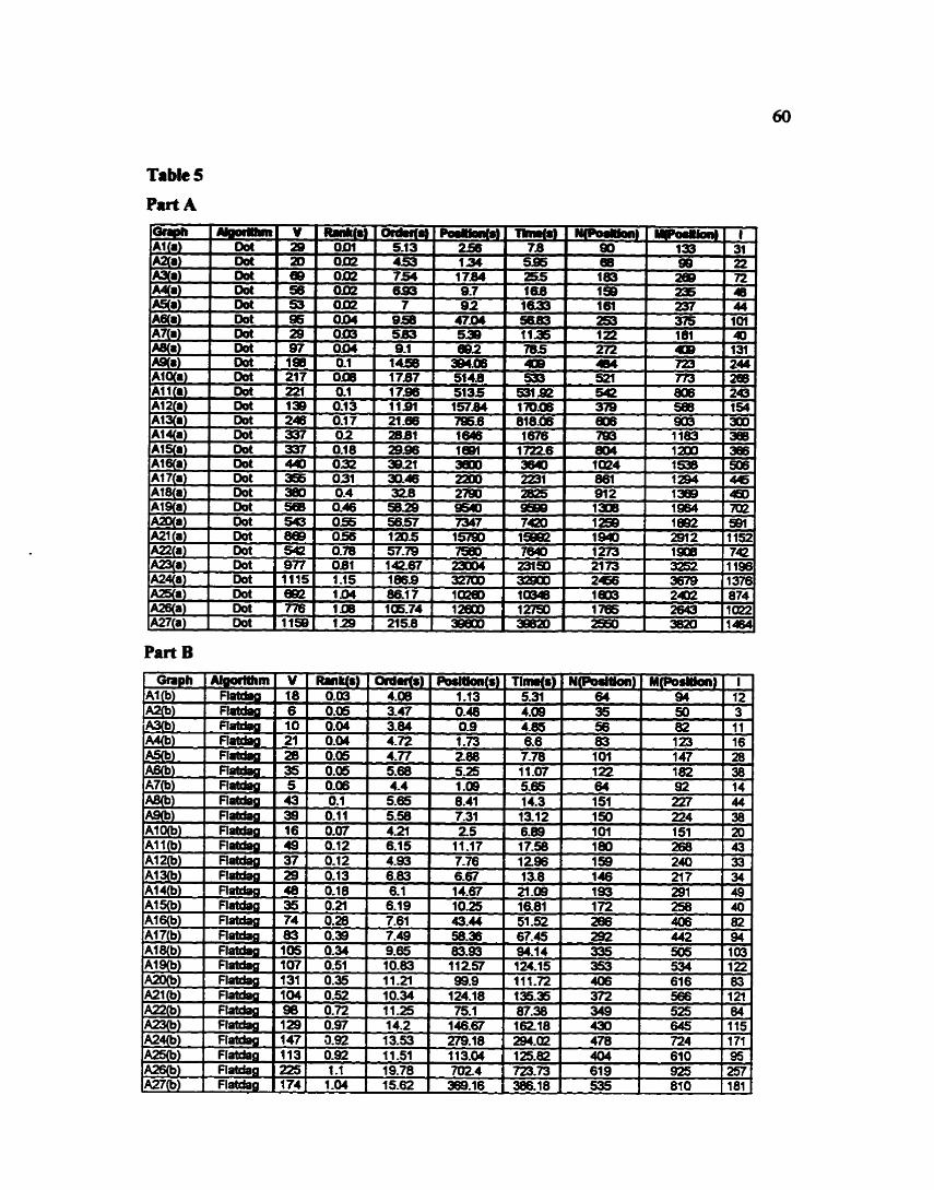
TI ble 5
P u t A
Part B
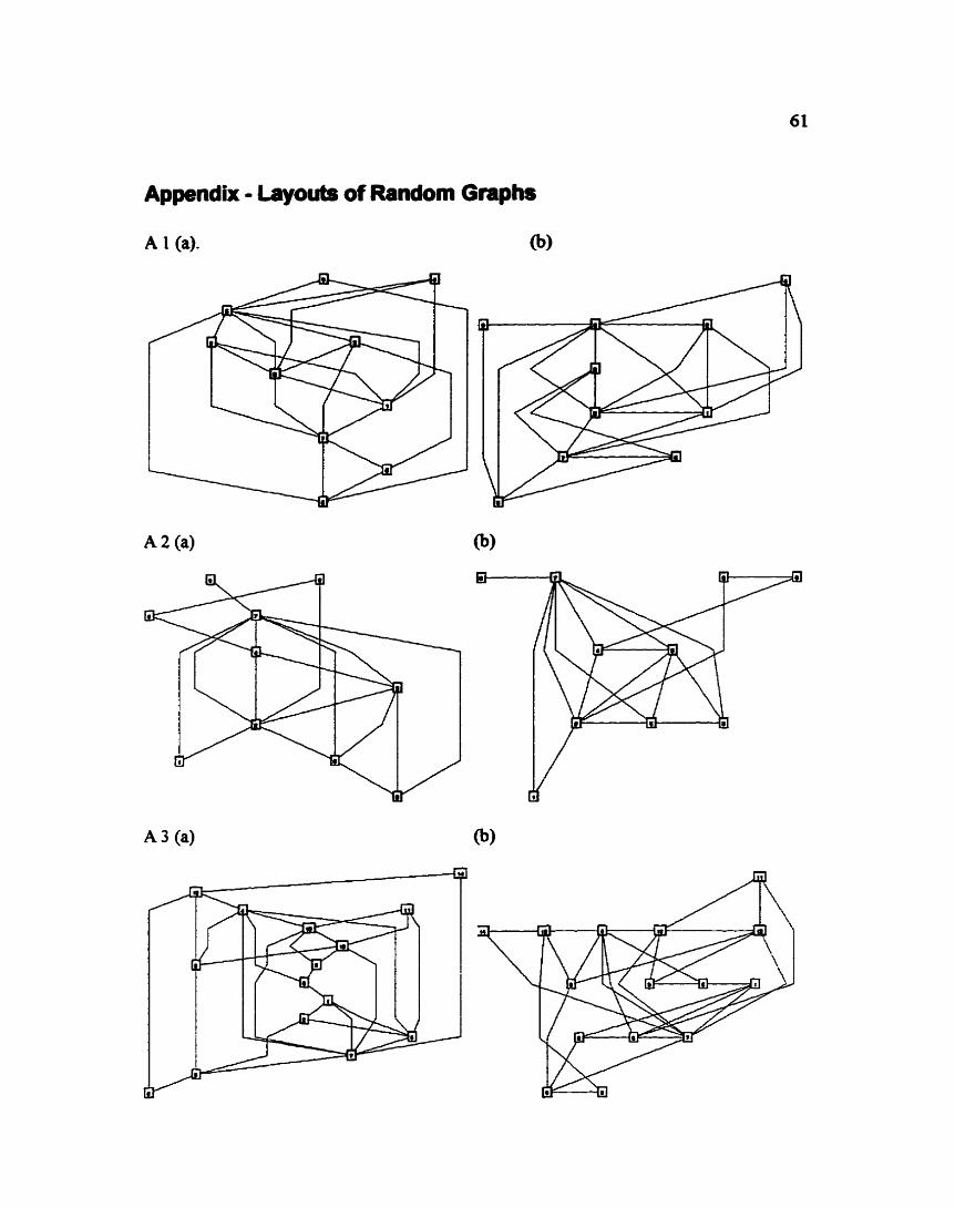
Appendix - Layouts of Random Graphs
A 1 (a).
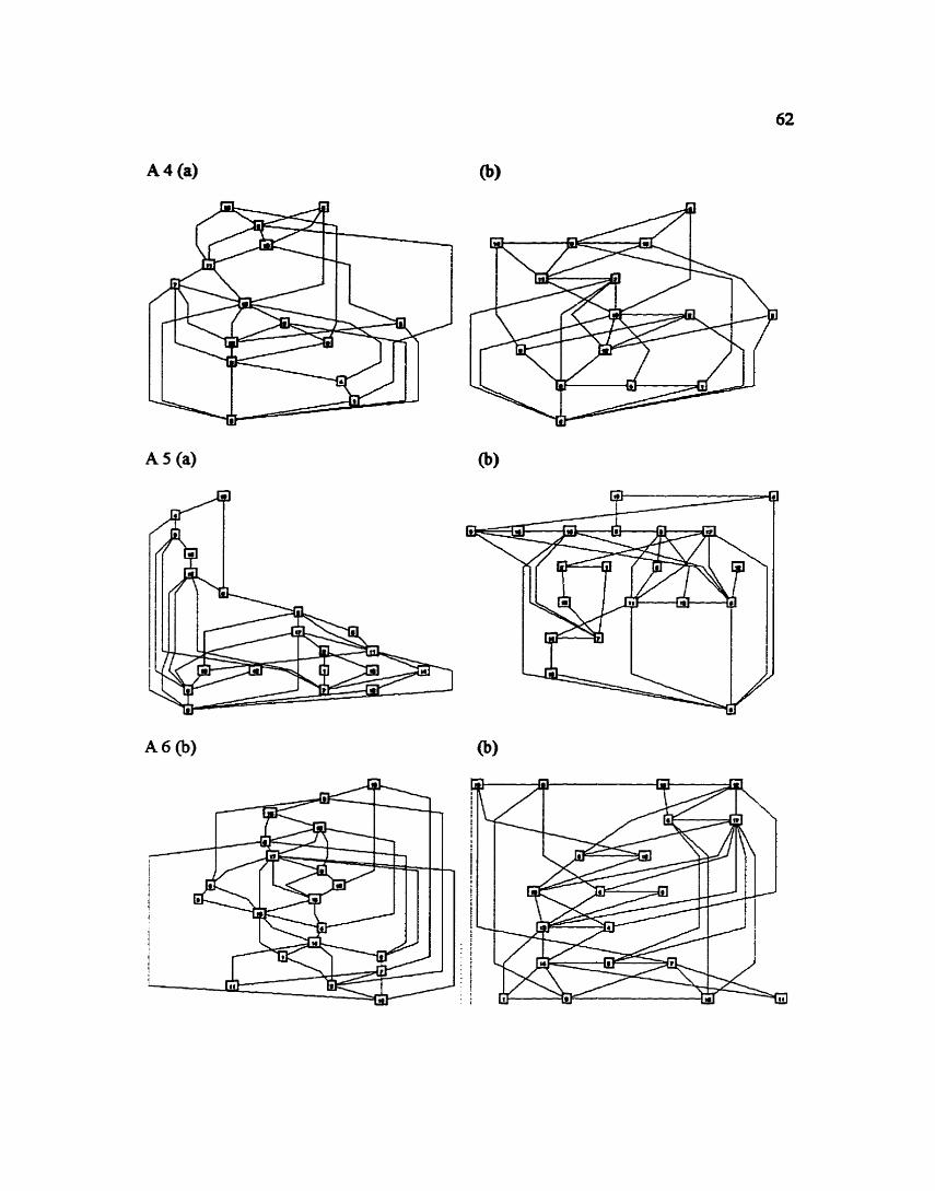
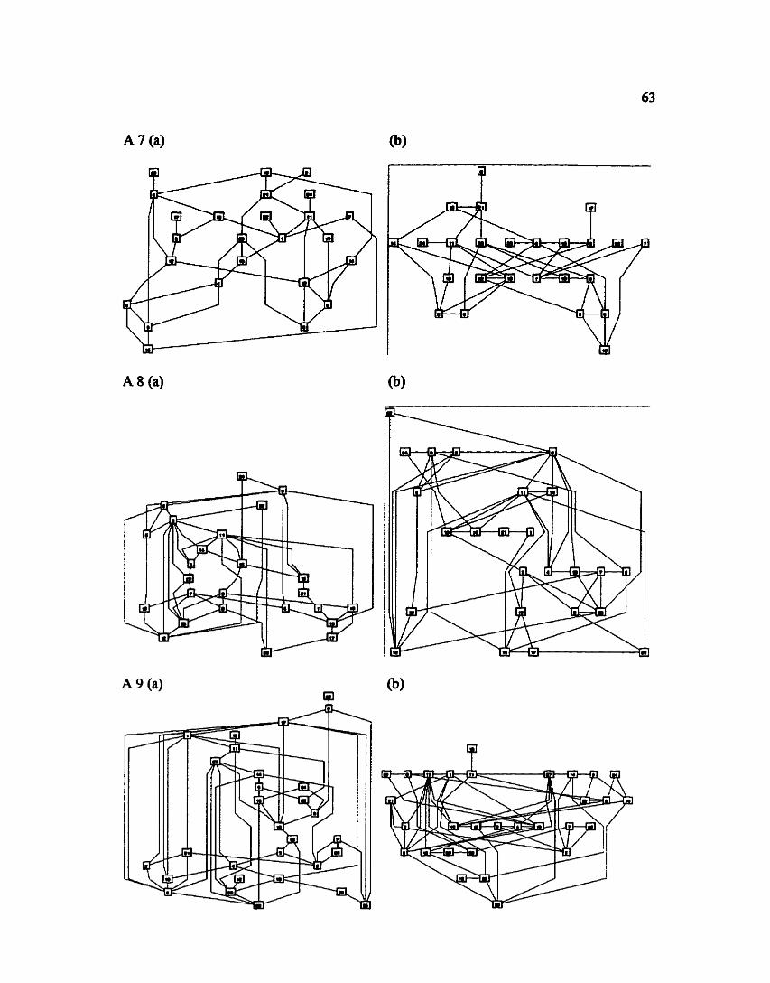
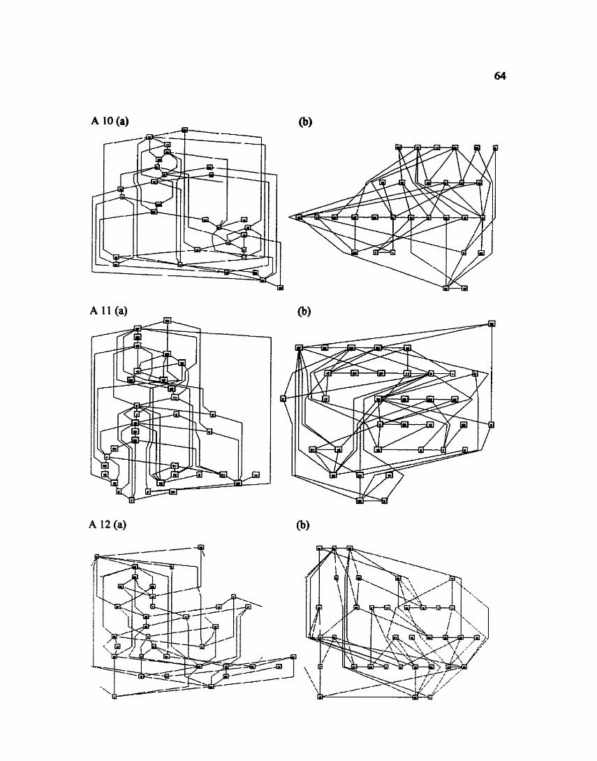
A I2 (a)
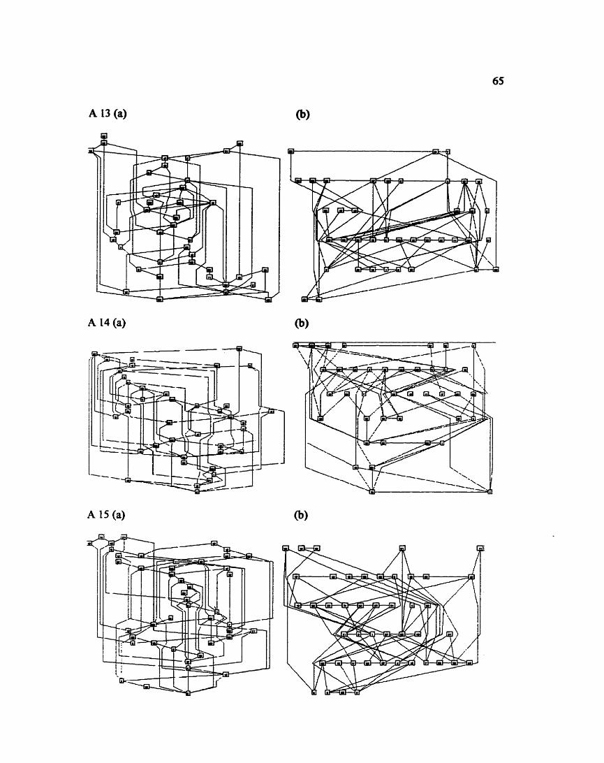
A 13 (a)
P
A 14 (a)
A IS (a)
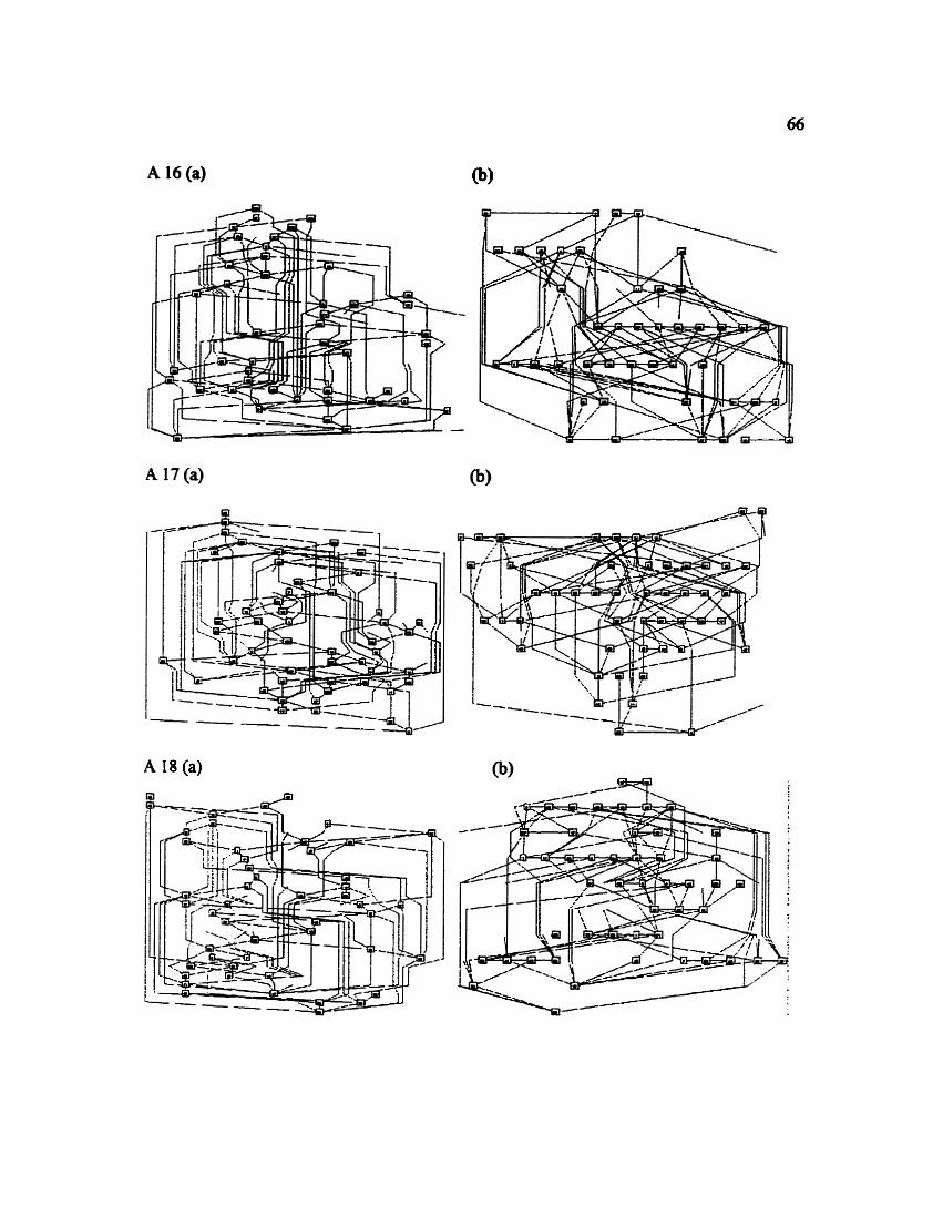
A 18 (a)
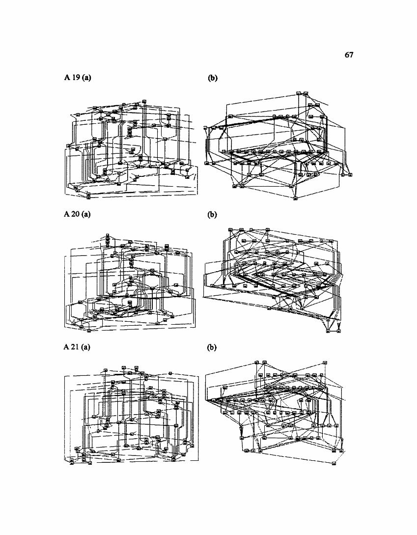
A 19 (a)
A 20 (a)
A 21 (a)
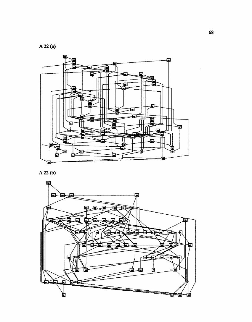
A 22 (a)
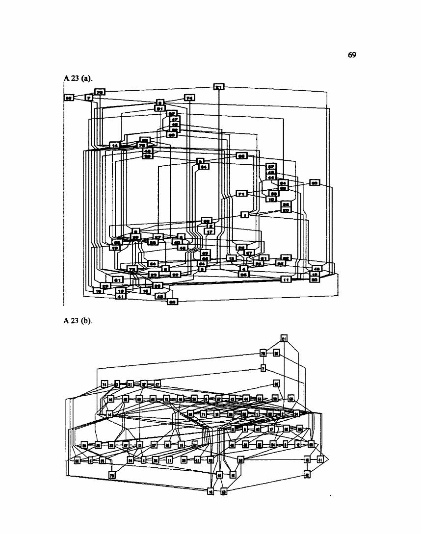
A 23 (b).
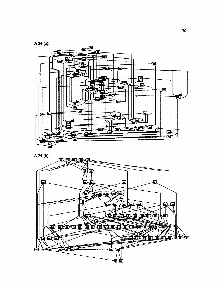
A 24 (a).
A 24 (b).
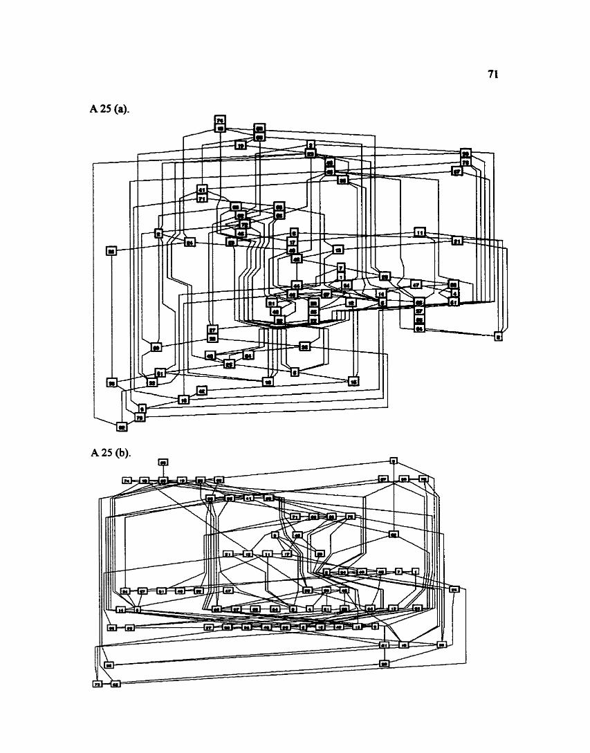
A 25 (a).
A 26 (b).

A 27 (a).
A 27 (b). C1
References
[BBL95] P. BertoIazzi, G. Di Battista, and G. Liotta, "Parametric Graph Drawing," IEEE Trmrs. on &@are Eqgheen'ng, vol. 21, no. 8, August 1995.
PBLM941 P. Bertolazzi, G. Di Battista, G. Liotta, and C. Mannho, "Upward Drawings of Triconnected Digraphsm, A&withrnica, Sp~ger-Verlag, 1994, pp. 476497.
PETT941 G. Di Batthta, P. Eades, R Tamassia and 1- G. Toms, "Algorithms for Drawing Graphs: an Annotated Bibliography", Cornputrrtrbll~~ol Geometry Zkory and Applcafibm, vol. 4,1994, pp. 235-282.
pT88] G. Di Battista, and R Tamassia, "Algorithms for Plane Representations of Acyclic Digraphs", Theoretid Compter Science, vol6 1 , 1988, pp. 175- 198.
[CARP801 M. J. Carpano, "Automatic Display of Hierarchized Graphs for Computer Aided Design Analysis," I ' Tram. on Systems, M i , md Cybernetics, vol. SMC- 1 0, no. 1 1,1980, pp. 705-715.
@5ADES86] P. Eades, B. McKay, and N. Wormald, "On an edge crossing problem," Proc 9th Austrahm Computer Science Conference, 1986, pp. 3 27-3 3 4.
WCK9q Arne Frick, "Upper Bounds on the Number of Hidden Nodes in the Sugiyarna Algorithm," Proceedings of Graph Drawing '96,1996.
[GEST47] W. Kohler, GestaIt PsychoZogy. New York: New American Library, 1947. [GKN88] E. R Gammer, S. C. North, and K. P. Vo, "DAG - A Program that Draws Directed Graphs," Sofrware Practice cadEqverience, vol. 18, no. 11, 1988, pp. 1047- 1062.
[GKNV93] E.R Gaasner, E. Koutsofios, S. North, K. Vo, "A Technique for Drawing Directed Graphs", I'EEE Transactions on Sofitwe EEngineerig, VoL 19, No. 3, March 1993.
[GRAY9 11 Peter Gray, PsychoIogy, Worth Publishers Inc., 199 1.
w 6 9 ] F. Hafafy, Graph meaty, Addison-Wesley, Reading, MA, 1969.
WEST831 k R G. Heesterman, Mabices and Simtpex Algorithms, Boston: D. Reidel Publishing, 1983.
[JOHNS961 David S. Johnson, "A Theoretician's Guide to the Experimental Analysis of Algorithms," AT&T Research, April 30, 1996.
FOSSS] C. KO* I. Marks, and S. Sbiebeq "Automating the Layout ofNetwork Diagrams with S-ed V i -on," IEEE Tram on Systems, Man, and Cybemtics, vol. 24, no. 3, March 1994.
-11 Eli B. Messinger7 Laweace A b w e 7 and Robert R Hemy, "A Divide-and- Conquer Algorithm for the Automatic Layout of Large Directed Graphs,'' llEE Tr~c t iorzs on sysf. Mmr Cybern. vol. 21, no. 1, January I Febnrary 199 1.
FORTH931 S. C. North, "Drawing Ranked Digraphs with R d e Clusters," AT&T Bell Laboratories, Nov. 3, 1993.
[STT8 I] K Sugiyama, S. Tagawa, and M. Toda, Methods for Yis11uI U'rsfandjing of Hierwchimi Systems, IEEE Trans. Systems, Man, and Cybernetics, vol SMC-I 1, n0.2, 1981, pp 109 - 125. [WARF77] J. Warfield, "Crossing theory and hierarchy mappings," ZEEE Tr- Syst. Ma. Cybem. vol. SMC-7 no. 7, July 1977, pp. 505-523.