A 2-Approximation algorithm for finding an optimum 3-Vertex-Connected Spanning Subgraph.
B.Sc. Engg. Thesis
An Algorithm for Finding Minimum Edge-Ranking
Spanning Tree
of Series-Parallel Graphs
by
Mohammad Atiqul Haque (0005031)
Md. Reaz Uddin (0005101)
Shajia Akhter Sharmin (0005072)
Submitted to
Department of Computer Science and Engineering
Bangladesh University of Engineering and Technology (BUET)
Dhaka 1000
November 2006
Dedication
To our Parents
i
Candidates’ Declaration
It is hereby declared that this thesis or any part of it has not been submitted
elsewhere for the award of any degree or diploma.
Mohammad Atiqul Haque
Md. Reaz Uddin
Shazia Akhter Sharmin
Candidates
ii
Contents
Candidate’s Declaration ii
Acknowledgements vii
Abstract 1
1 Introduction 2
1.1 Backgrounds . . . . . . . . . . . . . . . . . . . . . . . . . . . . . . . . 2
1.1.1 Edge-Ranking Problem . . . . . . . . . . . . . . . . . . . . . . 3
1.1.2 The Minimum Edge-Ranking Spanning Tree Problem . . . . . 4
1.1.3 Vertex-Ranking Problem . . . . . . . . . . . . . . . . . . . . . 5
1.1.4 The Minimum Vertex-Ranking Spanning Tree Problem . . . . 6
1.1.5 The Minimum Degree Spanning Tree Problem . . . . . . . . . 7
1.2 Applications . . . . . . . . . . . . . . . . . . . . . . . . . . . . . . . . 7
1.3 Scope of the thesis . . . . . . . . . . . . . . . . . . . . . . . . . . . . 8
1.3.1 Minimum Edge-Ranking Spanning Tree . . . . . . . . . . . . . 8
1.3.2 Minimum Degree Spanning Tree . . . . . . . . . . . . . . . . . 9
iii
CONTENTS iv
2 Preliminaries 11
2.1 Basic Definitions . . . . . . . . . . . . . . . . . . . . . . . . . . . . . 12
2.1.1 Graphs . . . . . . . . . . . . . . . . . . . . . . . . . . . . . . . 12
2.1.2 Degree of a Vertex . . . . . . . . . . . . . . . . . . . . . . . . 13
2.1.3 Subgraphs . . . . . . . . . . . . . . . . . . . . . . . . . . . . . 13
2.1.4 Connected Components . . . . . . . . . . . . . . . . . . . . . 14
2.1.5 Trees . . . . . . . . . . . . . . . . . . . . . . . . . . . . . . . . 15
2.1.6 Spanning Trees . . . . . . . . . . . . . . . . . . . . . . . . . . 16
2.2 Series-Parallel Graphs . . . . . . . . . . . . . . . . . . . . . . . . . . 16
2.2.1 Binary Decomposition Tree . . . . . . . . . . . . . . . . . . . 18
2.3 Edge-Ranking of Trees . . . . . . . . . . . . . . . . . . . . . . . . . . 19
2.4 Complexity of Algorithms . . . . . . . . . . . . . . . . . . . . . . . . 20
2.4.1 Complexity Classes: P and NP . . . . . . . . . . . . . . . . . 20
2.4.2 NP-Complete Problem . . . . . . . . . . . . . . . . . . . . . . 21
2.5 Approximation Algorithm and Approximation Ratio . . . . . . . . . . 22
3 Minimum Edge-Ranking Spanning Tree 24
3.1 Equivalence Class . . . . . . . . . . . . . . . . . . . . . . . . . . . . . 24
3.2 Algorithm for Minimum Edge-Ranking Spanning tree . . . . . . . . . 29
3.3 Conclusion . . . . . . . . . . . . . . . . . . . . . . . . . . . . . . . . . 33
4 Approximation Algorithm 34
4.1 Algorithm for Minimum Degree Spanning Tree . . . . . . . . . . . . . 35
CONTENTS v
4.2 Approximation Algorithm for Minimum Edge-Ranking Spanning Tree 40
4.3 Conclusion . . . . . . . . . . . . . . . . . . . . . . . . . . . . . . . . . 41
5 Conclusion 43
List of Figures
1.1 A graph G. . . . . . . . . . . . . . . . . . . . . . . . . . . . . . . . . 3
1.2 An optimal edge-ranking of graph G. . . . . . . . . . . . . . . . . . . 4
1.3 Edge contraction steps. . . . . . . . . . . . . . . . . . . . . . . . . . . 5
1.4 An optimal vertex-ranking of graph G. . . . . . . . . . . . . . . . . . 6
2.1 A graph G. . . . . . . . . . . . . . . . . . . . . . . . . . . . . . . . . 12
2.2 Subgraphs induced by vertices and edges of G. . . . . . . . . . . . . . 13
2.3 Components of a Graph . . . . . . . . . . . . . . . . . . . . . . . . . 14
2.4 A tree T . . . . . . . . . . . . . . . . . . . . . . . . . . . . . . . . . . 15
2.5 Series and parallel connection of a series-parallel graph. . . . . . . . . 17
2.6 A series-parallel graph and its binary decomposition tree. . . . . . . . 18
vi

Acknowledgments
All praises and thanks belong to Allah, the exalted for His innumerable favors and
bounties that only He knows the amount of. It is He who has granted us physical
and mental capabilities to complete the thesis work, without anything or anyone
compelling Him to do so.
We would love to express our solemn gratitude to our supervisor Dr. Md.
Abul Kashem Mia, Professor, Department of Computer Science and Engineering,
Bangladesh University of Engineering and Technology (BUET), Dhaka. His
supervision, encouragement and personal guidance were always with us during the
progress of the thesis. His concepts and problem solving approach have been very
helpful for the successful completion of this work. We are ever grateful to him.
We are thankful to all of our teachers and friends for their support during the
whole period of our thesis.
Finally, we remember our parents and family members who are always a source
of inspiration in every good action.
vii
Abstract
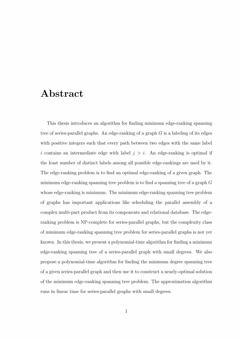
This thesis introduces an algorithm for finding minimum edge-ranking spanning
tree of series-parallel graphs. An edge-ranking of a graph G is a labeling of its edges
with positive integers such that every path between two edges with the same label
i contains an intermediate edge with label j > i. An edge-ranking is optimal if
the least number of distinct labels among all possible edge-rankings are used by it.
The edge-ranking problem is to find an optimal edge-ranking of a given graph. The
minimum edge-ranking spanning tree problem is to find a spanning tree of a graph G
whose edge-ranking is minimum. The minimum edge-ranking spanning tree problem
of graphs has important applications like scheduling the parallel assembly of a
complex multi-part product from its components and relational database. The edge-
ranking problem is NP-complete for series-parallel graphs, but the complexity class
of minimum edge-ranking spanning tree problem for series-parallel graphs is not yet
known. In this thesis, we present a polynomial-time algorithm for finding a minimum
edge-ranking spanning tree of a series-parallel graph with small degrees. We also
propose a polynomial-time algorithm for finding the minimum degree spanning tree
of a given series-parallel graph and then use it to construct a nearly-optimal solution
of the minimum edge-ranking spanning tree problem. The approximation algorithm
runs in linear time for series-parallel graphs with small degrees.
1
Chapter 1
Introduction
In this chapter, we provide the necessary background, present state and motivation
for this study on the rankings of graphs, define the problem and scope of this thesis.
In Section 1.1, we discuss the historical background on graph coloring. We also
define the vertex-ranking, edge-ranking , minimum vertex-ranking spanning tree
and minimum edge-ranking spanning tree problem. Section 1.2 represents some
applications of the minimum edge-ranking spanning tree problem. Section 1.3 deals
with the scope of this thesis.
1.1 Backgrounds
Graph theory is a delightful playground for the exploration of proof techniques in
discrete mathematics, and its results have applications in many areas of computing,
social and natural sciences. Recent research effort is concentrating on evolving
efficient algorithms in combinatorial mathematics especially graph theory.
Graph coloring theory not only plays an important role in discrete mathematics,
2
CHAPTER 1. INTRODUCTION 3
but also is of interest for its applications. Graph coloring deals with the fundamental
problem of partitioning a set of objects into classes according to certain rules.
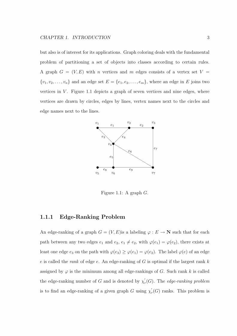
A graph G = (V,E) with n vertices and m edges consists of a vertex set V =
{v1, v2, . . . , vn} and an edge set E = {e1, e2, . . . , em}, where an edge in E joins two
vertices in V . Figure 1.1 depicts a graph of seven vertices and nine edges, where
vertices are drawn by circles, edges by lines, vertex names next to the circles and
edge names next to the lines.
e6
v4
v5
e8v6
e9v7
e7
v3e2
v2e1
v1
e3
e5
e4
Figure 1.1: A graph G.
1.1.1 Edge-Ranking Problem
An edge-ranking of a graph G = (V, E)is a labeling ϕ : E → N such that for each
path between any two edges e1 and e2, e1 6= e2, with ϕ(e1) = ϕ(e2), there exists at
least one edge e3 on the path with ϕ(e3) ≥ ϕ(e1) = ϕ(e2). The label ϕ(e) of an edge
e is called the rank of edge e. An edge-ranking of G is optimal if the largest rank k
assigned by ϕ is the minimum among all edge-rankings of G. Such rank k is called
the edge-ranking number of G and is denoted by χ′r(G). The edge-ranking problem
is to find an edge-ranking of a given graph G using χ′r(G) ranks. This problem is
CHAPTER 1. INTRODUCTION 4
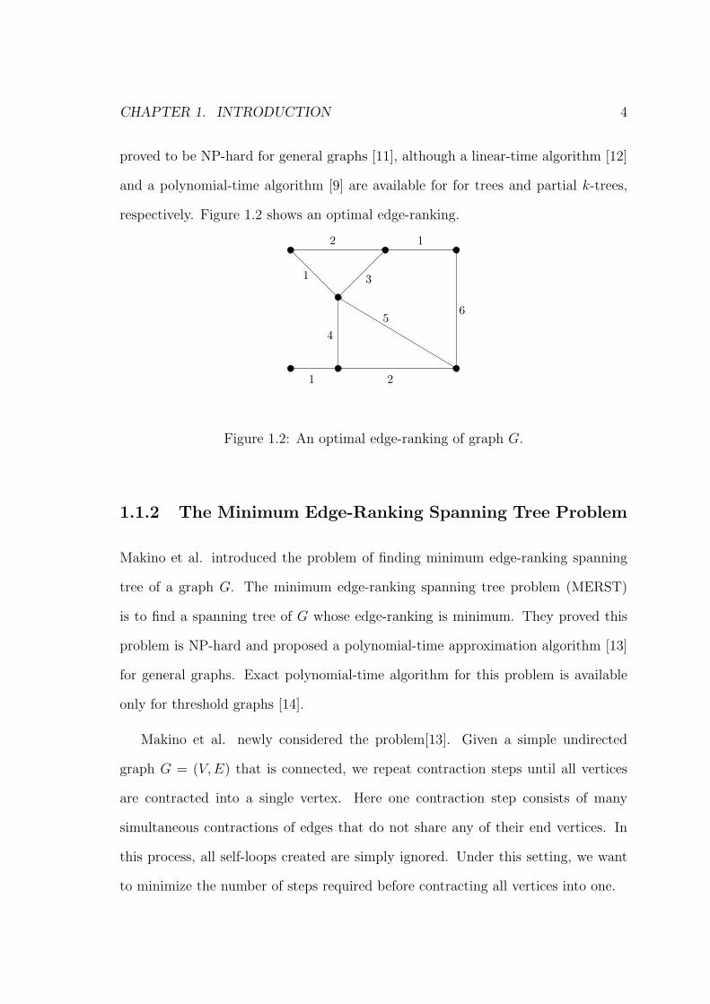
proved to be NP-hard for general graphs [11], although a linear-time algorithm [12]
and a polynomial-time algorithm [9] are available for for trees and partial k-trees,
respectively. Figure 1.2 shows an optimal edge-ranking.
1
45
6
31
12
2
Figure 1.2: An optimal edge-ranking of graph G.
1.1.2 The Minimum Edge-Ranking Spanning Tree Problem
Makino et al. introduced the problem of finding minimum edge-ranking spanning
tree of a graph G. The minimum edge-ranking spanning tree problem (MERST)
is to find a spanning tree of G whose edge-ranking is minimum. They proved this
problem is NP-hard and proposed a polynomial-time approximation algorithm [13]
for general graphs. Exact polynomial-time algorithm for this problem is available
only for threshold graphs [14].
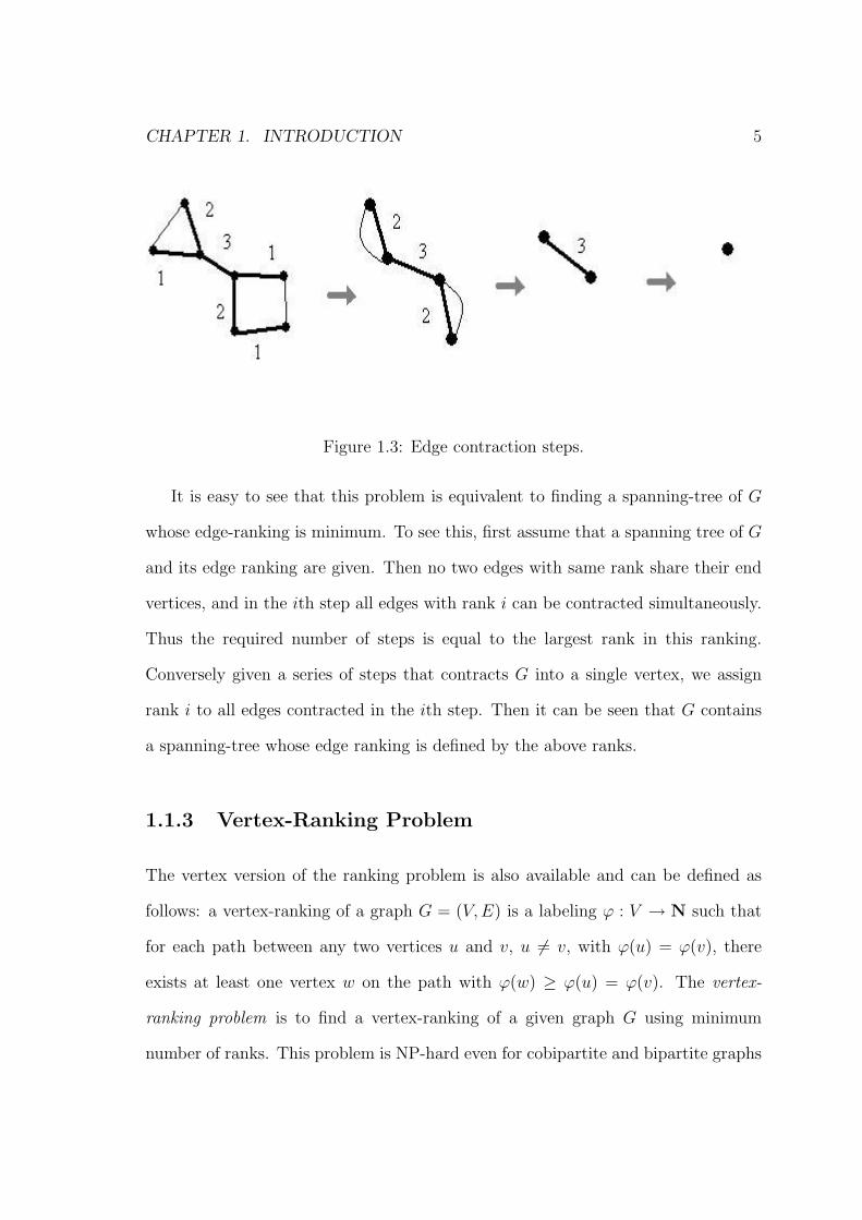
Makino et al. newly considered the problem[13]. Given a simple undirected
graph G = (V,E) that is connected, we repeat contraction steps until all vertices
are contracted into a single vertex. Here one contraction step consists of many
simultaneous contractions of edges that do not share any of their end vertices. In
this process, all self-loops created are simply ignored. Under this setting, we want
to minimize the number of steps required before contracting all vertices into one.
CHAPTER 1. INTRODUCTION 5
Figure 1.3: Edge contraction steps.
It is easy to see that this problem is equivalent to finding a spanning-tree of G
whose edge-ranking is minimum. To see this, first assume that a spanning tree of G
and its edge ranking are given. Then no two edges with same rank share their end
vertices, and in the ith step all edges with rank i can be contracted simultaneously.
Thus the required number of steps is equal to the largest rank in this ranking.
Conversely given a series of steps that contracts G into a single vertex, we assign
rank i to all edges contracted in the ith step. Then it can be seen that G contains
a spanning-tree whose edge ranking is defined by the above ranks.
1.1.3 Vertex-Ranking Problem
The vertex version of the ranking problem is also available and can be defined as
follows: a vertex-ranking of a graph G = (V,E) is a labeling ϕ : V → N such that
for each path between any two vertices u and v, u 6= v, with ϕ(u) = ϕ(v), there
exists at least one vertex w on the path with ϕ(w) ≥ ϕ(u) = ϕ(v). The vertex-
ranking problem is to find a vertex-ranking of a given graph G using minimum
number of ranks. This problem is NP-hard even for cobipartite and bipartite graphs
CHAPTER 1. INTRODUCTION 6
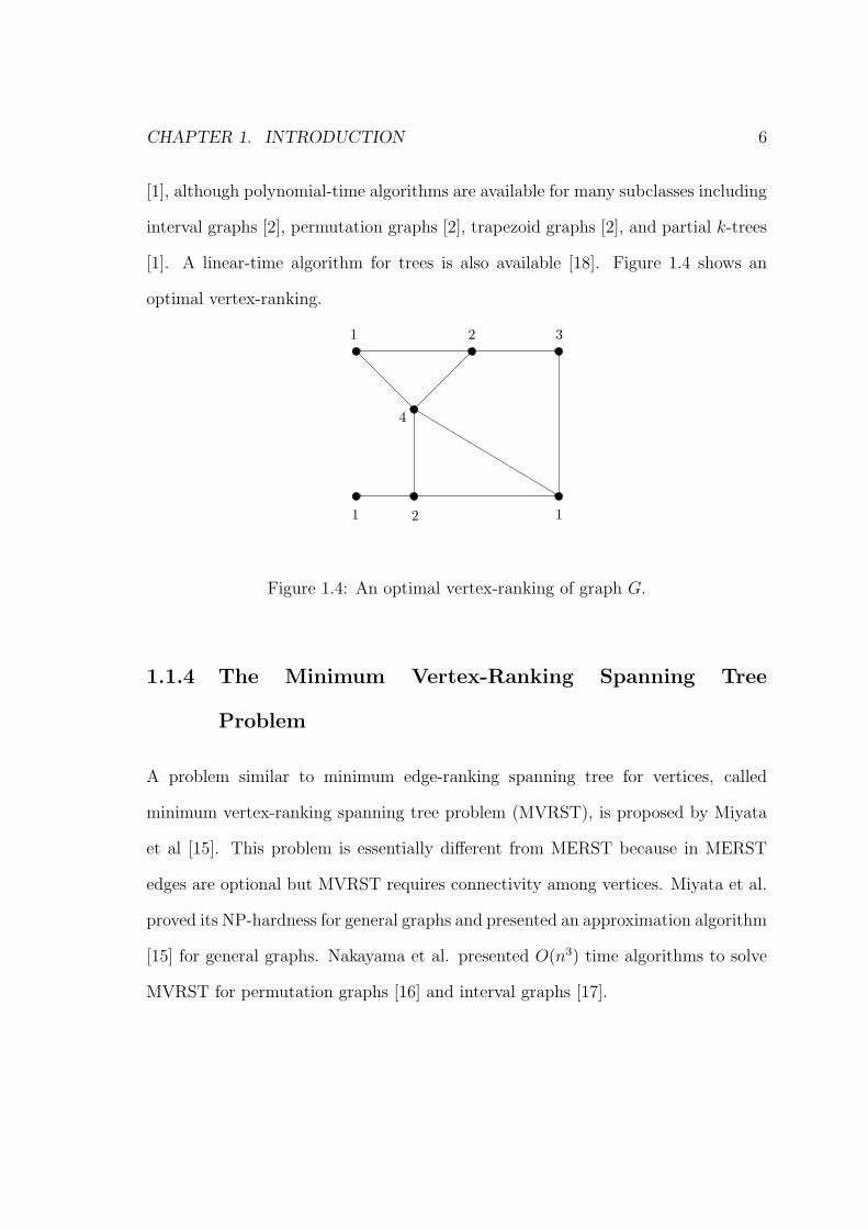
[1], although polynomial-time algorithms are available for many subclasses including
interval graphs [2], permutation graphs [2], trapezoid graphs [2], and partial k-trees
[1]. A linear-time algorithm for trees is also available [18]. Figure 1.4 shows an
optimal vertex-ranking.
1
1 12
4
32
Figure 1.4: An optimal vertex-ranking of graph G.
1.1.4 The Minimum Vertex-Ranking Spanning Tree
Problem
A problem similar to minimum edge-ranking spanning tree for vertices, called
minimum vertex-ranking spanning tree problem (MVRST), is proposed by Miyata
et al [15]. This problem is essentially different from MERST because in MERST
edges are optional but MVRST requires connectivity among vertices. Miyata et al.
proved its NP-hardness for general graphs and presented an approximation algorithm
[15] for general graphs. Nakayama et al. presented O(n3) time algorithms to solve
MVRST for permutation graphs [16] and interval graphs [17].
CHAPTER 1. INTRODUCTION 7
1.1.5 The Minimum Degree Spanning Tree Problem
A minimum degree spanning tree of a graph G = (V, E) is a spanning tree of G
whose maximum degree, ∆ is the smallest among all spanning trees of G. The
problem minimum degree spanning tree (MDST) is to find such a spanning tree of
G. It is a generalization of the Hamiltonian Path problem and thus is also NP-hard.
MDST problem has many practical applications including computation of spanning
trees in dynamic networks for non-critical broadcast and designing power grids [3].
1.2 Applications
Minimum edge-ranking spanning tree problem has some interesting applications
specially in the field of networking, multipart assembly and relational database.
Makino et al. has presented some practical applications [13]. Consider a network
of web sites, where data are stored in different sites. In order to derive some new
information from them, we want to merge a set of relevant data into one site. During
the merging process, the pertaining data must be locked to avoid the interventions
from others, such as being overwritten, and therefore no data can participate in
more than one merging process at the same time. However, pairs of data can be
merged simultaneously if they do not share any data. It is now not difficult to see
that the minimization of the completion time of this merging process is formulated
as minimum edge-ranking spanning tree problem.
Another example is found in relational database theory. Let us consider the
“query graph”, where its vertex set corresponds to a set of relations and its edge
set represents the pairs of relations that are joined. In this context, join operations
that are represented by nonadjacent edges can be joined parallel, but no two join
CHAPTER 1. INTRODUCTION 8
operations corresponding to adjacent edges can be performed simultaneously, since
a relation can participate only in one join operation at a time. The join operations
are then performed until all relations come into a single relational table. The whole
process can again be modeled as MERST.
Another example is scheduling the parallel assembly of multipart product from its
components. Given a set of connections of its components to be combined in order
to complete the product, we aim to minimize the number of steps of combining
components in parallel under the condition that any component cannot be used in
more than on combining step at a time.
1.3 Scope of the thesis
This thesis deals with the problem of finding minimum edge-ranking spanning tree
of series-parallel graph. We present an optimal and an approximation algorithm for
solving the problem. This Thesis also provides an optimal algorithm for solving the
minimum degree spanning-tree problem of a series parallel graph, which is used in
the approximation algorithm.
1.3.1 Minimum Edge-Ranking Spanning Tree
In This thesis we introduce an optimal algorithm for solving the minimum edge-
ranking spanning tree (MERST) problem for series-parallel graphs.The edge-ranking
problem on series-parallel graphs is already proved to be NP-complete [7]. But the
complexity bound of the minimum edge-ranking spanning tree problem on series-
parallel graphs is not known yet. Neither it is proved to be NP-complete, nor a
polynomial-time algorithm is available. In this thesis, we propose an algorithm
CHAPTER 1. INTRODUCTION 9
which runs in O(n4∆+1∆4(log n)4) time for series-parallel graphs. Thus for small
degrees, the algorithm runs in polynomial time.
We use the algorithm for minimum degree spanning tree problem to construct
an approximation algorithm to solve minimum edge-ranking spanning tree problem.
The approximate algorithm runs in O(n∆4log ∆). For small degrees, the algorithm
runs in linear time. This restriction is indeed practical for ordinary series-parallel
graphs.
1.3.2 Minimum Degree Spanning Tree
The best available approximation algorithm for solving MDST is due to Furer and
Raghavachari [4]. They provided a polynomial-time algorithm to approximate the
MDST problem to within one of optimal. Their algorithm also extends to the Steiner
version of the problem. Their algorithm runs in O(mn log nα(n)), where m is the
number of edges and α is the inverse Ackerman function. Gavish [5] formulated the
MDST problem as a mixed integer program and provided an exact solution using
the method of Lagrangian multipliers.
A variant of MDST for directed graphs (DMDST) is also available. It can be
defined as follows: consider a directed graph G = (V, E) with n vertices and a
root vertex r ∈ V . The DMDST problem for G is one of constructing a spanning
tree rooted at r, whose maximal degree is the smallest among all such spanning
trees. The problem is known to be NP-hard. R. Krishnan and B. Raghavachari
[10] proposes an approximation algorithm that finds a spanning tree whose maximal
degree is at most O(∆∗+log n) where, ∆∗ is the degree of some optimal tree for the
problem. Their algorithm runs in quasi-polynomial time O(nO(log n)).
CHAPTER 1. INTRODUCTION 10
In this thesis we consider the undirected version of MDST that is minimum
degree spanning tree for series parallel graphs. We propose an algorithm that solves
the problem which runs in O(n∆4log ∆) time for series-parallel graphs. Thus the
algorithm runs in linear time for series-parallel graphs with small degrees.
Chapter 2
Preliminaries
In this chapter, we define some basic definitions and some special types of graphs.
Definitions that are not given here are discussed as they are needed. In Section 2.1,
we start by giving the definitions of some basic terms of graph which are related
to and used through out this thesis. Section 2.2 defines a special type of graph,
series-parallel graph. It also introduces different properties of a series-parallel graph
and representation of series-parallel graph through the binary decomposition tree.
Section 2.3 presents the upper and lower bound of edge-ranking of trees. Section
2.4 discusses complexity classes of the algorithm. Finally in Section 2.5 we define
approximation algorithm and the approximation ratio.
11
CHAPTER 2. PRELIMINARIES 12
2.1 Basic Definitions
2.1.1 Graphs
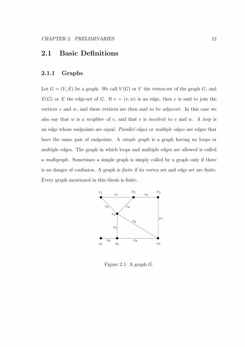
Let G = (V, E) be a graph. We call V (G) or V the vertex-set of the graph G, and
E(G) or E the edge-set of G. If e = (v, w) is an edge, then e is said to join the
vertices v and w, and these vertices are then said to be adjacent . In this case we
also say that w is a neighbor of v, and that e is incident to v and w. A loop is
an edge whose endpoints are equal. Parallel edges or multiple edges are edges that
have the same pair of endpoints. A simple graph is a graph having no loops or
multiple edges. The graph in which loops and multiple edges are allowed is called
a multigraph. Sometimes a simple graph is simply called by a graph only if there
is no danger of confusion. A graph is finite if its vertex set and edge set are finite.
Every graph mentioned in this thesis is finite.
e6
v4
v5
e8v6
e9v7
e7
v3e2
v2e1
v1
e3
e5
e4
Figure 2.1: A graph G.
CHAPTER 2. PRELIMINARIES 13
2.1.2 Degree of a Vertex
The degree of a vertex v in a graph G is the number of edges incident to v, and is
denoted by d(v). The maximum degree of G is denoted by ∆(G) or simply by ∆.
In Figure 2.1, the degree of vertex d(v1) v1 is 2 and the maximum degree ∆ of G, is
4 as d(v4) is 4.
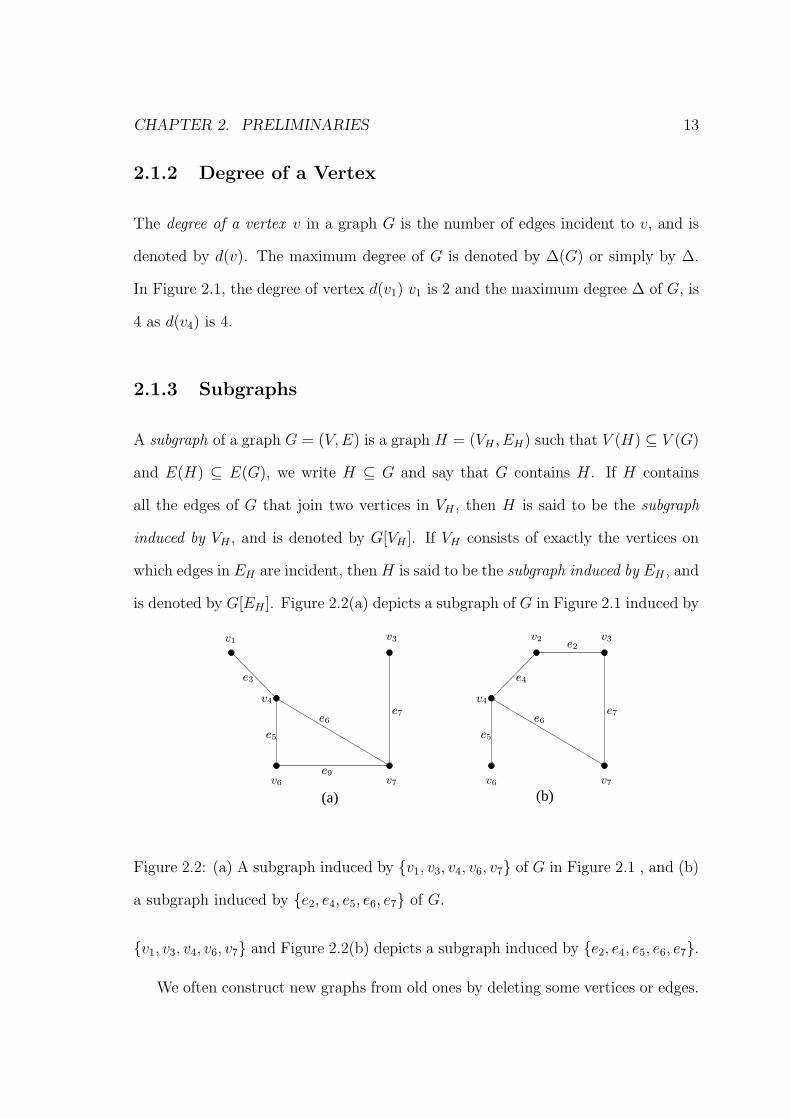
2.1.3 Subgraphs
A subgraph of a graph G = (V,E) is a graph H = (VH , EH) such that V (H) ⊆ V (G)
and E(H) ⊆ E(G), we write H ⊆ G and say that G contains H. If H contains
all the edges of G that join two vertices in VH , then H is said to be the subgraph
induced by VH , and is denoted by G[VH ]. If VH consists of exactly the vertices on
which edges in EH are incident, then H is said to be the subgraph induced by EH , and
is denoted by G[EH ]. Figure 2.2(a) depicts a subgraph of G in Figure 2.1 induced by
(b)(a)
e6
v4
v6
e9v7
e7
v3v1
e3
e5
e6
e4
e5
v2e2
v3
e7
v7v6
v4
Figure 2.2: (a) A subgraph induced by {v1, v3, v4, v6, v7} of G in Figure 2.1 , and (b)
a subgraph induced by {e2, e4, e5, e6, e7} of G.
{v1, v3, v4, v6, v7} and Figure 2.2(b) depicts a subgraph induced by {e2, e4, e5, e6, e7}.
We often construct new graphs from old ones by deleting some vertices or edges.
CHAPTER 2. PRELIMINARIES 14
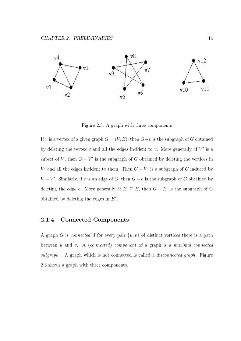
Figure 2.3: A graph with three components
If v is a vertex of a given graph G = (V, E), then G−v is the subgraph of G obtained
by deleting the vertex v and all the edges incident to v. More generally, if V ′ is a
subset of V , then G− V ′ is the subgraph of G obtained by deleting the vertices in
V ′ and all the edges incident to them. Then G− V ′ is a subgraph of G induced by
V − V ′. Similarly, if e is an edge of G, then G− e is the subgraph of G obtained by
deleting the edge e. More generally, if E ′ ⊆ E, then G − E ′ is the subgraph of G
obtained by deleting the edges in E ′.
2.1.4 Connected Components
A graph G is connected if for every pair {u, v} of distinct vertices there is a path
between u and v. A (connected) component of a graph is a maximal connected
subgraph . A graph which is not connected is called a disconnected graph. Figure
2.3 shows a graph with three components.
CHAPTER 2. PRELIMINARIES 15
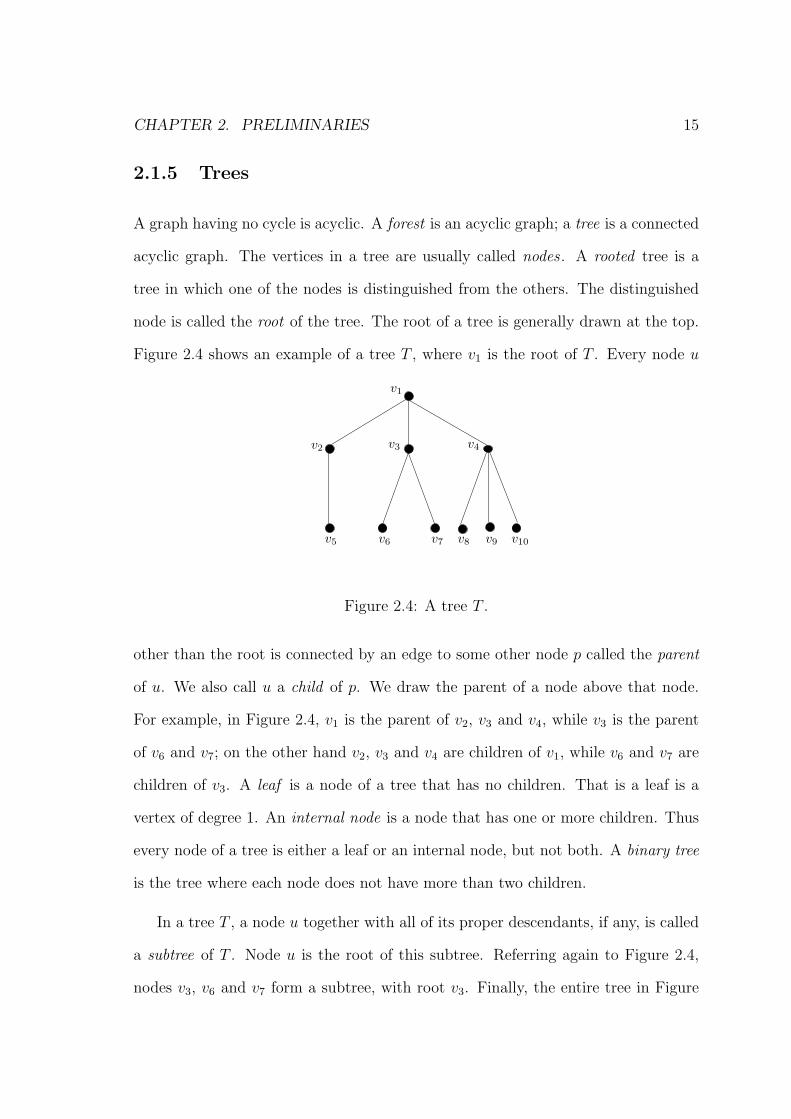
2.1.5 Trees
A graph having no cycle is acyclic. A forest is an acyclic graph; a tree is a connected
acyclic graph. The vertices in a tree are usually called nodes . A rooted tree is a
tree in which one of the nodes is distinguished from the others. The distinguished
node is called the root of the tree. The root of a tree is generally drawn at the top.
Figure 2.4 shows an example of a tree T , where v1 is the root of T . Every node u
v1
v9 v10v8v7v6v5
v4v3v2
Figure 2.4: A tree T .
other than the root is connected by an edge to some other node p called the parent
of u. We also call u a child of p. We draw the parent of a node above that node.
For example, in Figure 2.4, v1 is the parent of v2, v3 and v4, while v3 is the parent
of v6 and v7; on the other hand v2, v3 and v4 are children of v1, while v6 and v7 are
children of v3. A leaf is a node of a tree that has no children. That is a leaf is a
vertex of degree 1. An internal node is a node that has one or more children. Thus
every node of a tree is either a leaf or an internal node, but not both. A binary tree
is the tree where each node does not have more than two children.
In a tree T , a node u together with all of its proper descendants, if any, is called
a subtree of T . Node u is the root of this subtree. Referring again to Figure 2.4,
nodes v3, v6 and v7 form a subtree, with root v3. Finally, the entire tree in Figure
CHAPTER 2. PRELIMINARIES 16
2.4 is a subtree of itself, with root v1. The height of a node u in a tree is the length
of a longest path from u to a leaf. The height of a tree is the height of the root.
The depth of a node u in a tree is the length of a path from the root to u. The level
of a node u in a tree is the height of the tree minus the depth of u. In Figure 2.4,
for example, node v3 is of height 1, depth 1 and level 1. The tree in Figure 2.4 has
height 2.
2.1.6 Spanning Trees
A spanning tree is a spanning subgraph that is a tree. A spanning subgraph of a
graph G is a subgraph with vertex set V (G)
2.2 Series-Parallel Graphs
Let G = (V, E) be a graph with vertex set V and edge set E. The set of vertices
and the set of edges of G are often denoted by V (G) and E(G), respectively. A
(two-terminal) series-parallel graph is defined recursively as follows.
1. A graph G of a single edge is a series-parallel graph. The ends vs and vt of
the edge are called the terminals of G and denoted by vs(G) and vt(G).
2. Let Gy be a series-parallel graph with terminals vs(Gy) and vt(Gy), and let Gz
be a series-parallel graph with terminals vs(Gz) and vt(Gz).
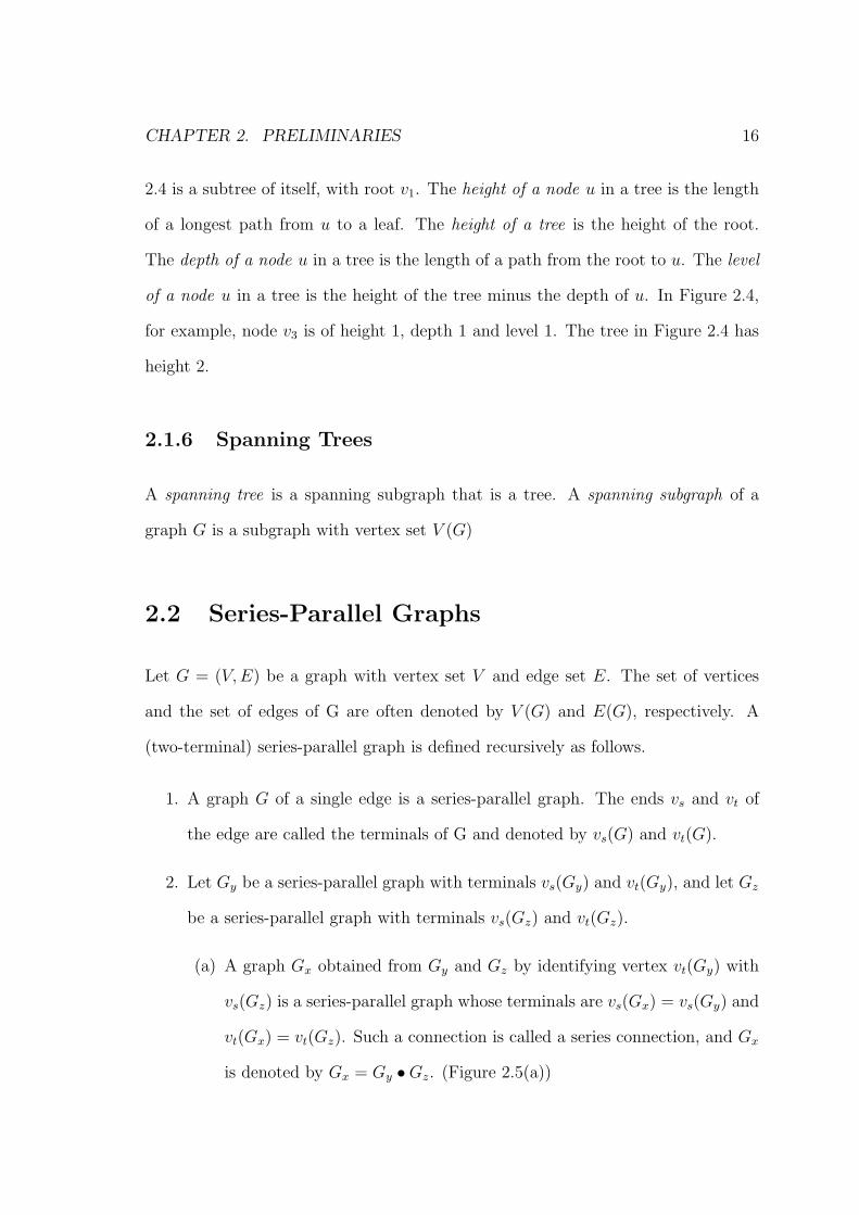
(a) A graph Gx obtained from Gy and Gz by identifying vertex vt(Gy) with
vs(Gz) is a series-parallel graph whose terminals are vs(Gx) = vs(Gy) and
vt(Gx) = vt(Gz). Such a connection is called a series connection, and Gx
is denoted by Gx = Gy •Gz. (Figure 2.5(a))
CHAPTER 2. PRELIMINARIES 17
(b) A graph Gx obtained from Gy and Gz by identifying vertex vs(Gy) with
vs(Gz) and vt(Gy) with vt(Gz) is a series-parallel graph whose terminals
are vs(Gx) = vs(Gy) = vs(Gz) and vt(Gx) = vt(Gy) = vt(Gz). Such a
connection is called a parallel connection and Gx is denoted by Gx =
Gy‖Gz. (Figure 2.5(b))
(b)
(a)
t = t1 = t2
s = s1 = s2
s2
G
t1 t2s1
G2
t2s2
G1
s1 t1
t
s
G
G1 G2
t1
s1s1
t2
s2
=
Figure 2.5: A series-parallel graph G composed from G1 and G2 (a) with series
connection, and (b) with parallel connection.
The terminals vs(Gx) and vt(Gx) are often denoted shortly by vs and vt
respectively.
CHAPTER 2. PRELIMINARIES 18
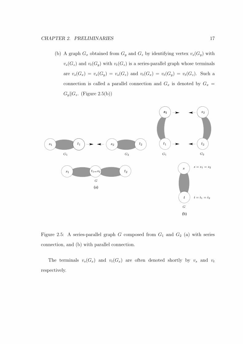
Figure 2.6: A series-parallel graph and its binary decomposition tree.
2.2.1 Binary Decomposition Tree
A series-parallel graph can be represented by a “binary decomposition tree” [1].
Figure 2.6(a) illustrates a series-parallel graph G and Figure 2.6(b) shows its binary
decomposition tree Tb. Labels s and p attached to internal nodes in Tb indicate
series and parallel connections, respectively, and nodes labeled s and p are called s-
and p- nodes, respectively.
Let Tb = (Vb, Eb) be a binary decomposition tree of a series-parallel graph G.
Let Tb(x) be the subtree of Tb rooted at node x. Every leaf x of Tb represents a
subgraph of G induced by two vertices vs and vt connected by an edge ex = (vs, vt).
We associate a subgraph Gx = (Vx, Ex) of G with each node x of tree Tb, where
Vx =⋃{Sy | y = x or y is a descendant of x in T}, and
Ex = {ey | y is a leaf node in T (x)}.
Here Sx = {vs, vt} is the set of terminals of Gx. The graph associated with the root
of T is the graph G itself. A spanning forest of a graph Gx is an acyclic subgraph
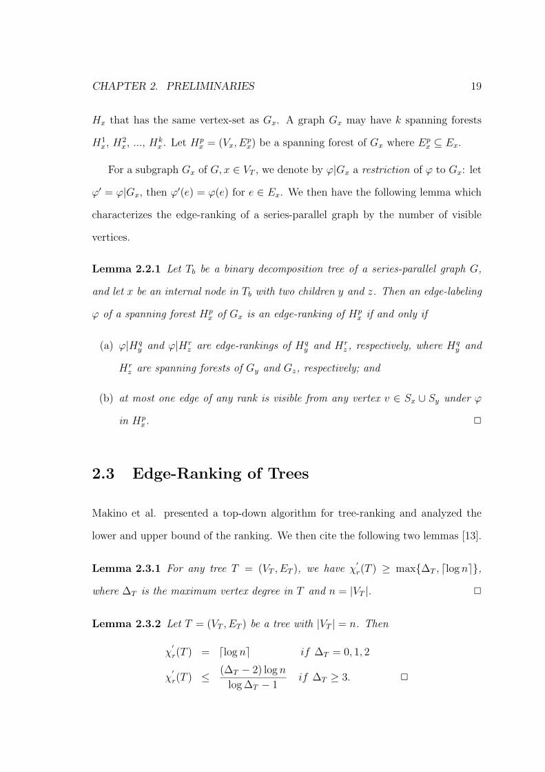
CHAPTER 2. PRELIMINARIES 19
Hx that has the same vertex-set as Gx. A graph Gx may have k spanning forests
H1x, H2
x, ..., Hkx . Let Hp
x = (Vx, Epx) be a spanning forest of Gx where Ep
x ⊆ Ex.
For a subgraph Gx of G, x ∈ VT , we denote by ϕ|Gx a restriction of ϕ to Gx: let
ϕ′ = ϕ|Gx, then ϕ′(e) = ϕ(e) for e ∈ Ex. We then have the following lemma which
characterizes the edge-ranking of a series-parallel graph by the number of visible
vertices.
Lemma 2.2.1 Let Tb be a binary decomposition tree of a series-parallel graph G,
and let x be an internal node in Tb with two children y and z. Then an edge-labeling
ϕ of a spanning forest Hpx of Gx is an edge-ranking of Hp
x if and only if
(a) ϕ|Hqy and ϕ|Hr
z are edge-rankings of Hqy and Hr
z , respectively, where Hqy and
Hrz are spanning forests of Gy and Gz, respectively; and
(b) at most one edge of any rank is visible from any vertex v ∈ Sx ∪ Sy under ϕ
in Hpx. 2
2.3 Edge-Ranking of Trees
Makino et al. presented a top-down algorithm for tree-ranking and analyzed the
lower and upper bound of the ranking. We then cite the following two lemmas [13].
Lemma 2.3.1 For any tree T = (VT , ET ), we have χ′r(T ) ≥ max{∆T , dlog ne},
where ∆T is the maximum vertex degree in T and n = |VT |. 2
Lemma 2.3.2 Let T = (VT , ET ) be a tree with |VT | = n. Then
χ′r(T ) = dlog ne if ∆T = 0, 1, 2
χ′r(T ) ≤ (∆T − 2) log n
log ∆T − 1if ∆T ≥ 3. 2
CHAPTER 2. PRELIMINARIES 20
Proofs of these lemmas are presented by Makino et al. [13].
2.4 Complexity of Algorithms
The efficiency or complexity of an algorithm is determined by the amount of
resources (such as time and storage) necessary to execute it. Generally, it is defined
as a function relating the input length n to the number of steps (time complexity) or
storage locations (space or memory complexity) required to execute the algorithm.
In theoretical analysis of algorithms it is common to estimate their complexity in
asymptotic sense, i.e., to estimate the complexity function for reasonably large
length of input n. For example, since binary search is said to run an amount of
steps proportional to a logarithm, its complexity of the running time is defined by
O(log(n)). If the running time of an algorithm is bounded by O(n), it is said to be
a linear-time algorithm.
2.4.1 Complexity Classes: P and NP
A problem is said to have a polynomial-time algorithm if the worst case running
time is O(nk) for input size n and for some constant k. Generally, problems that
are solvable by polynomial-time algorithms are tractable or easy, and problems that
require superpolynomial time are intractable or hard. Based upon the running time
of algorithms, next we define complexity classes. The class P consists of all those
decision problems that can be solved on a deterministic sequential machine in an
amount of time that is polynomial in the size of the input; the class NP consists of
all those problems whose positive solutions can be verified in polynomial time given
the right information, or equivalently, whose solution can be found in polynomial
CHAPTER 2. PRELIMINARIES 21
time on a non-deterministic machine. Any problem in P is also in NP , since if a
problem is in P then we can verify it in polynomial time.
2.4.2 NP-Complete Problem
Here, we are mainly interested in another class of problems, called NP-complete
problems (or NPC), which can be loosely described as the hardest problems in NPand therefore they are the least likely to be in P . No polynomial-time algorithm
has yet been discovered for an NP-complete problem, nor has anyone yet been able
to prove that no polynomial-time algorithm can exist for any of them.
More precisely, a decision problem C is NP-complete if it is complete for NP ,
meaning that:
(1) it is in NP , and
(2) it is NP-hard , i.e. every other problem in NP is polynomial-time reducible
to it.
“Polynomial-time reducible” here means that for every problem L, there is a
polynomial-time many-one reduction, a deterministic algorithm which transforms
instances l ∈ L into instances c ∈ C, such that the answer to c is YES if and only if
the answer to l is YES. To prove that an NP problem A is in fact an NP-complete
problem it is sufficient to show that an already knownNP-complete problem reduces
to A. A consequence of this definition is that if we had a polynomial-time algorithm
for C, we could solve all problems in NP in polynomial time.
CHAPTER 2. PRELIMINARIES 22
2.5 Approximation Algorithm and
Approximation Ratio
At present, all known algorithms for NP-complete problems require time that is
superpolynomial in the input size. It is unknown whether there are any faster
algorithms. Therefore, to solve an NP-complete problem for any nontrivial problem
size, generally it may still be possible to find near-optimal solutions in polynomial
time. An algorithm that quickly finds a suboptimal solution that is within a certain
(known) range of the optimal one is called an approximation algorithm.
Depending on the problem, maximization or minimization, an optimal solution
may be defined as one with maximum possible cost or one with minimum possible
cost. An approximation ratio is a measure of goodness of the approximation solution
with the optimal solution of the problem. An algorithm for a problem has an
approximation ratio of ρ(n) if, for any input size n, the cost C of the solution
produced by the algorithm is within factor of ρ(n) of the cost C∗ of an optimal
solution:
max
{C
C∗ ,C∗
C
}(2.1)
An algorithm that achieves an approximation ratio of ρ(n) is called ρ(n)-
approximation algorithm. For a maximization problem, 0 < C ≤ C∗, and the ratio
C∗/C gives the factor by which the cost of an optimal solution is larger than the cost
of the approximate solution. Similarly, for a minimization problem, 0 < C∗ ≤ C,
and the ratio C/C∗ gives the factor by which the cost of an approximate solution
is larger than the cost of the optimal solution. Since all solutions are assumed
CHAPTER 2. PRELIMINARIES 23
to have positive cost, these ratios are always well defined. The approximation
ratio of an approximation algorithm is never less than 1, since C/C∗ < 1 implies
C∗/C > 1. Therefore, a 1-approximation algorithm produces an optimal solution,
and an approximation algorithm with a large approximation ratio may return a
solution that is much worse than optimal.
Chapter 3
Minimum Edge-Ranking Spanning
Tree
This chapter presents our optimal algorithm for finding the minimum edge-ranking
spanning tree of series-parallel graphs. Section 3.1 describes the equivalence class
used in the algorithm to reduce the table size required to hold the intermediate
solutions. In section 3.2 the algorithm and its time complexity is discussed. Finally,
section 3.3 summarizes the chapter.
3.1 Equivalence Class
Our algorithm uses dynamic programming. On each node of the decomposition tree
of the input graph a table of all possible partial solutions of the problem is computed.
The complexity of the algorithm depends on the size of the table. So we need to
find an appropriate equivalence class to reduce the table size. Before defining the
equivalence class, we need to define a few terms.
24
CHAPTER 3. MINIMUM EDGE-RANKING SPANNING TREE 25
Let ϕ be an edge-labeling of a series-parallel graph. G = (V, E). The label
(rank) of an edge e ∈ E is denoted by ϕ(e). The number of ranks used by an edge-
labeling ϕ is denoted by #ϕ. Without loss of generality it can be assumed that ϕ
uses consecutive integers 1, 2, · · · , #ϕ as the ranks. The rank of an edge e ∈ E is
said to be visible from a vertex v ∈ V under ϕ in G if G has a path P from v to e
every edge of which has a rank ≤ ϕ(e).
Let Tb be the decomposition tree of the series-parallel graph G = (V, E). Let
R = {1, 2, · · · ,m} be the set of ranks. Let x be a node in Tb. Let ϕ : Ex → R be an
edge-ranking of a spanning forest Hpx = (Vx, E
px) of G. Iyer et al introduced the idea
of “critical list” to solve the ordinary vertex-ranking problem for trees [6]. Later
similar idea was used to define visible-list L(ϕ, v) [8, 20, 21]. We use the similar
concept for edge-ranking and define visible-list L(ϕ, v) as:
L(ϕ, v) = {ϕ(e)|e ∈ Ex is visible from a vertex v under ϕ in Hpx}.
For an integer i we denote by count(L(ϕ, v), i) the number of visible vertices
with rank i. For a list L and an integer l, we define a sublist [L ≥ l] of L as follows:
[L ≥ l] = {i ∈ L|i ≥ l}.
Now we define obstacle λϕ, λϕ ∈ R ∪ {∞}, in a path from vs to vt as follows:
λϕ = max{ϕ(e)| e is an edge on the path P from vs to vt in Hpx}.
Let λϕ = ∞ if Hpx has no path from vs to vt. If (vs, vt) ∈ Ep
x, then λϕ = ϕ(e) where
e = (vs, vt). If an edge e ∈ Epx is visible from vt and ϕ(e) ≥ λϕ, then the edge is also
visible from vs. We next define a visible list-set L(ϕ) and a vector R(ϕ) for Hpx as
follows [8]:
L(ϕ) = {L(ϕ, vs), L(ϕ, vt)}, and
CHAPTER 3. MINIMUM EDGE-RANKING SPANNING TREE 26
R(ϕ) = (L(ϕ), λϕ, tϕ).
Here we use a parameter tϕ because we keep two types of solution at each node
x ∈ VT . A one-tree type solution is an edge-ranking of a spanning tree of Gx. A
two-tree type solution is an edge-ranking of a spanning forest of Gx with exactly
two components(trees). Let tϕ = 1 and tϕ = 2 for one-tree type and two-tree type
solution respectively. We call such a pair R(ϕ) the vector of ϕ on node x. R(ϕ) is
called feasible vector if the edge-labeling ϕ is an edge ranking of Gx. An edge-ranking
ϕ of Gx, x ∈ VT , is defined to be extensible if it can be extended to an edge-ranking
ϕ′ of G without changing the labeling of edges in Gx. Then ϕ = ϕ′|Gx. We then
have the following lemma.
Lemma 3.1.1 Let ϕ and η be two edge-rankings of the same spanning forest or two
different forests of Gx such that R(ϕ) = R(η). Then ϕ is extensible if and only if η
is extensible.
Proof. Let ϕ and η are two edge-rankings of two different spanning forests
Hpx = (Vx, E
px) and Hq
x = (Vx, Eqx) of Gx. It suffices to prove that if ϕ is extensible
then η is extensible. Let V ∗ = V − Vx and let G∗ be the subgraph of G induced by
V ∗ and let H∗ = (V ∗, E∗) be the spanning forest of G∗. Assume that ϕ is extensible.
Then ϕ can be extended to an edge-ranking ϕ′ of spanning tree Hp = (Hpx ∪H∗) of
G = (V, E) such that ϕ′(e) = ϕ(e) for any edge e ∈ Ex. Let n(G,ϕ, i) be the number
of edges in E(G) having rank i for the edge-ranking ϕ. Extend the edge-ranking η
of Hqx to a edge-labeling η′ of spanning tree Hq = (Hq
x ∪H∗) as follows:
η′(e) =
η(e) if e ∈ Ex; and
ϕ′(e) if e ∈ E∗.
CHAPTER 3. MINIMUM EDGE-RANKING SPANNING TREE 27
Now it suffices to prove that η′ is a valid edge-ranking of spanning tree Hq, that is
n(Fη′ , η′, i) ≤ 1 for any rank i ∈ R and for any connected component Fη′ = (Vη′ , Eη′)
of the graph obtained from Hq by deleting all the edges e ∈ E with η′(e) > i. Then
there are following two cases to consider:
Case 1: Fη′ has no vertex in Sx.
In this case, Fη′ is a subgraph of either H∗ or Hqx since H∗ is connected to Hq
x only
through vertices in Sx. Moreover η′|H∗ = ϕ′|H∗ and η′|Hqx = η are edge-rankings of
H∗ and Hqx respectively. Therefore n(Fη′ , η
′, i) ≤ 1.
Case 2: Fη′ has a vertex w in Sx.
Let e ∈ Eη′ is an edge adjacent to w and e has the smallest rank of all edges adjacent
to w under η′. In this case, obviously η′(e) ≤ i. If e ∈ E∗ then η′(e) = ϕ′(e) ≤ i.
On the other hand if e ∈ Eqx then smallest rank in L(η, w) is η(e) ≤ i. Since
R(ϕ) = R(η) we have L(η, w) = L(ϕ,w). So smallest rank in L(ϕ,w) equal to
η(e). Hence, there must be an edge having rank equal to η(e) ≤ i adjacent to
w under ϕ. In both cases there is an edge adjacent to w having rank ≤ i under
ϕ′. So deletion of all edges e ∈ E with ϕ′(e) > i from Hp leaves a connected
component Fϕ′ = (Vϕ′ , Eϕ′) containing the vertex w. Since ϕ′ is valid ranking of Hp,
n(Fϕ′ , ϕ′, i) ≤ 1. Therefore, it suffices to prove that n(Fη′ , η
′, i) = n(Fϕ′ , ϕ′, i).
Since η′|H∗ = ϕ′|H∗ one can observe that Vη′ ∩ V ∗ = Vϕ′ ∩ V ∗ although Vη′ ∩ Vx =
Vϕ′ ∩ Vx does not necessarily hold. Let Fη be the subgraph of Fη′ induced by
Vη′ ∩ Vx and F ∗η′ be the subgraph of Fη′ induced by (Vη′ ∩ V ∗) ∪ {w}. Similarly,
let Fϕ be the subgraph of Fϕ′ induced by Vϕ′ ∩ Vx and F ∗ϕ′ be the subgraph of
Fϕ′ induced by (Vϕ′ ∩ V ∗) ∪ {w}. Then n(Fη′ , η′, i) = n(Fη, η, i) + n(F ∗
η′ , η′, i) and
n(Fϕ′ , ϕ′, i) = n(Fϕ, ϕ, i) + n(F ∗
ϕ′ , ϕ′, i). Since (Vη′ ∩ V ∗) ∪ {w} = (Vϕ′ ∩ V ∗) ∪ {w}
CHAPTER 3. MINIMUM EDGE-RANKING SPANNING TREE 28
and η′|H∗ = ϕ′|H∗ we have n(F ∗η′ , η
′, i) = n(F ∗ϕ′ , ϕ
′, i). Therefore it suffices to prove
that n(Fη, η, i) = n(Fϕ, ϕ, i)
We next show that each of the connected components of Fη and Fϕ contains at
least one vertex of Sx. Suppose for a contradiction that a connected component
D of Fη or Fϕ, say Fη, contains no vertex in Sx. Since Fη′ is a connected graph
containing w ∈ Sx, w is connected to a vertex of D by a path in Fη′ . However, it is
impossible because D has no vertex in Sx and Fη is connected with F ∗η′ only through
the vertices in Sx.
Let vs ∈ V (Fη) ∩ Sx = V (Fϕ) ∩ Sx. Let Dη be the connected component of Fη
that contains vs, and let Dϕ be the connected component of Fϕ that contains vs.
There are the following three cases to consider:
Case 2.1: tϕ = tη = 1 and λϕ = λη ≤ i.
In this case vs and vt are connected both in Hpx and Hq
x. No edge in the connecting
path has rank > i. So vs and vt must belong to the same component of Fη and Fϕ.
Hence {vs, vt} ∈ V (Dη) and {vs, vt} ∈ V (Dϕ).
Case 2.2: tϕ = tη = 1 and λϕ = λη > i.
Deleting vertices with rank > i from Hp and Hq breaks the path between vs and vt
in Hpx and Hq
x . So vs and vt cannot be in same component. Hence neither Dη nor
Dϕ contains vt.
Case 2.3: tϕ = tη = 2.
There is no path between vs and vt in Hpx or Hq
x. So vs and vt cannot be in same
component. Hence both Dη and Dϕ contain only vs.
Considering all the cases we have proved that V (Dη) ∩ Sx = V (Dϕ) ∩ Sx.
Clearly n(Dη, η, i) = count(L(η, vs), i) and n(Dϕ, ϕ, i) = count(L(ϕ, vs), i). Since
CHAPTER 3. MINIMUM EDGE-RANKING SPANNING TREE 29
L(η, vs) = L(ϕ, vs), we have count(L(η, vs), i) = count(L(ϕ, vs), i) and hence
n(Dη, η, i) = n(Dϕ, ϕ, i).
Thus we have proved that Fη and Fϕ have the same number of connected
components Dηjand Dϕj, for 1 ≤ j ≤ 2, respectively. Furthermore, one
may assume that n(Dηj, η, i) = n(Dϕj
, ϕ, i) for each j, 1 ≤ j ≤ 2. Since
n(Fη, η, i) =∑2
j=1 n(Dηj, η, i) and n(Fϕ, ϕ, i) =
∑2j=1 n(Dϕj
, ϕ, i), we have
n(Fη, η, i) = n(Fϕ, ϕ, i).
We have proved that whenever ϕ and η are edge-rankings of two different
spanning sub-graphs of Gx, then ϕ is extensible if and only if η is extensible.
Similarly we can prove that ϕ is extensible if and only if η is extensible when ϕ
and η are two edge-rankings of the same spanning forest of Gx. 2
3.2 Algorithm for Minimum Edge-Ranking
Spanning tree
We construct a minimum edge-ranking spanning tree of a graph recursively. We
follow a bottom-up approach. For a node x in the binary decomposition tree Tb
of the series-parallel graph G we generate all possible one-tree and two-tree type
solutions for the graph obtained by the subtrees rooted at that node. For a leaf
x ∈ Tb, we find one-tree type solutions by ranking the edge in x. On the other hand,
we find two-tree type solution considering the two vertices without the edge between
them. Let y and z be the two children of an internal node x ∈ Tb. For a s-node x,
an one-tree type solution of y combining with an one-tree type solution of z yields
an one-tree type solution for x. Again, an one-tree type solution of y combining
CHAPTER 3. MINIMUM EDGE-RANKING SPANNING TREE 30
with a two-tree type solution of z or a two-tree type solution of y combining with
an one-tree type solution of z results in a two-tree type solution for x. On the other
hand, if x is a p-node, an one-tree type solution of y combining with a two-tree
type solution of z or a two-tree type solution of y combining with an one-tree type
solution of z yields an one-tree type solution for x. Again, a two-tree type solution
of y combining with a two-tree type solution of z results in a two-tree type solution
for x. In the next two lemmas we show the updating process of vectors.
Lemma 3.2.1 Let Gx = Gy •Gz, let vs and v be the terminals of Gy, and v and vt
be the terminals of Gz. Let η and ψ be two edge-rankings of spanning forests Hqy and
Hrz of Gy and Gz, respectively. Let ϕ be the edge-labeling of a spanning forest of Gx
extended from η and ψ. Let the vectors of Hpx, Hq
y and Hrz be R(ϕ) = (L(ϕ), λϕ, tϕ),
R(η) = (L(η), λη, tη), and R(ψ) = (L(ψ), λψ, tψ), respectively. Then
L(ϕ, vs) =
L(η, vs) ∪ [L(ψ, v) ≥ λη] if tη = 1 and tψ = 1 or 2,
L(η, vs) if tη = 2 and tψ = 1.
L(ϕ, vt) =
L(ψ, vt) ∪ [L(η, v) ≥ λψ] if tη = 1 or 2 and tψ = 1,
L(ψ, vt) if tη = 1 and tψ = 2.
λϕ =
max{λη, λψ} if tη = 1 and tψ = 1,
∞ otherwise. 2
Lemma 3.2.2 Let Gx = Gy||Gz, let vs and vt be the terminals of Gy and Gz. Let η
and ψ be the edge-rankings of spanning forests Hqy and Hr
z of Gy and Gz, respectively.
Let ϕ be the edge-labeling of a spanning forest of Gx extended from η and ψ. Let
the vectors of Hpx, Hq
y and Hrz be R(ϕ) = (L(ϕ), λϕ, tϕ), R(η) = (L(η), λη, tη), and
CHAPTER 3. MINIMUM EDGE-RANKING SPANNING TREE 31
R(ψ) = (L(ψ), λψ, tψ), respectively. Then
L(ϕ, vs) =
L(η, vs) ∪ L(ψ, vs) ∪ [L(ψ, vt) ≥ λη] if tη = 1 and tψ = 2,
L(η, vs) ∪ L(ψ, vs) ∪ [L(η, vt) ≥ λψ] if tη = 2 and tψ = 1,
L(η, vs) ∪ L(ψ, vs) if tη = tψ = 2.
L(ϕ, vt) =
L(η, vt) ∪ L(ψ, vt) ∪ [L(ψ, vs) ≥ λη] if tη = 1 and tψ = 2,
L(η, vt) ∪ L(ψ, vt) ∪ [L(η, vs) ≥ λψ] if tη = 2 and tψ = 1,
L(η, vt) ∪ L(ψ, vt) if tη = tψ = 2.
λϕ =
λη if tη = 1
λψ if tψ = 1
∞ otherwise. 2
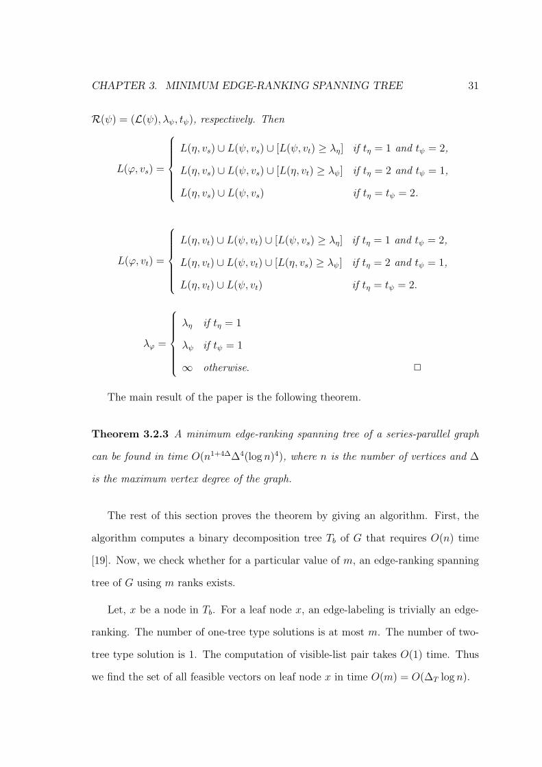
The main result of the paper is the following theorem.
Theorem 3.2.3 A minimum edge-ranking spanning tree of a series-parallel graph
can be found in time O(n1+4∆∆4(log n)4), where n is the number of vertices and ∆
is the maximum vertex degree of the graph.
The rest of this section proves the theorem by giving an algorithm. First, the
algorithm computes a binary decomposition tree Tb of G that requires O(n) time
[19]. Now, we check whether for a particular value of m, an edge-ranking spanning
tree of G using m ranks exists.
Let, x be a node in Tb. For a leaf node x, an edge-labeling is trivially an edge-
ranking. The number of one-tree type solutions is at most m. The number of two-
tree type solution is 1. The computation of visible-list pair takes O(1) time. Thus
we find the set of all feasible vectors on leaf node x in time O(m) = O(∆T log n).
CHAPTER 3. MINIMUM EDGE-RANKING SPANNING TREE 32
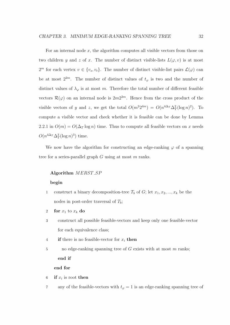
For an internal node x, the algorithm computes all visible vectors from those on
two children y and z of x. The number of distinct visible-lists L(ϕ, v) is at most
2m for each vertex v ∈ {vs, vt}. The number of distinct visible-list pairs L(ϕ) can
be at most 22m. The number of distinct values of tϕ is two and the number of
distinct values of λϕ is at most m. Therefore the total number of different feasible
vectors R(ϕ) on an internal node is 2m22m. Hence from the cross product of the
visible vectors of y and z, we get the total O(m224m) = O(n4∆T ∆2T (log n)2). To
compute a visible vector and check whether it is feasible can be done by Lemma
2.2.1 in O(m) = O(∆T log n) time. Thus to compute all feasible vectors on x needs
O(n4∆T ∆3T (log n)3) time.
We now have the algorithm for constructing an edge-ranking ϕ of a spanning
tree for a series-parallel graph G using at most m ranks.
Algorithm MERST SP
begin
1 construct a binary decomposition-tree Tb of G; let x1, x2, ..., xk be the
nodes in post-order traversal of Tb;
2 for x1 to xk do
3 construct all possible feasible-vectors and keep only one feasible-vector
for each equivalence class;
4 if there is no feasible-vector for xi then
5 no edge-ranking spanning tree of G exists with at most m ranks;
end if
end for
6 if xi is root then
7 any of the feasible-vectors with tϕ = 1 is an edge-ranking spanning tree of
CHAPTER 3. MINIMUM EDGE-RANKING SPANNING TREE 33
G
with at most m ranks;
end.
Line 1 can be done in O(n) time [19]. As explained above, line 3 can be done in
O(n4∆T ∆3T (log n)3) time for each execution. Line 3 is executed O(n) times. So, the
algorithm MERST SP requires O(n1+4∆T ∆3T (log n)3) time. Since 1 ≤ m ≤ ∆T log n
and ∆T ≤ ∆ by lemma 4.2.3, the minimum edge ranking spanning tree of a graph can
be constructed in O(n1+4∆∆4(log n)4) time. This completes the proof of Theorem
4.1.
3.3 Conclusion
In this chapter we present an algorithm for solving the minimum edge-ranking
spanning tree (MERST) problem on series-parallel graphs. This is the first
polynomial-time algorithm for MERST problem on series-parallel graphs with small
degrees. We simulated the algorithm by writing C++ program and ran the program
on a large number of graph data-sets. The simulation results have shown that the
algorithm properly rank the edges of the input graph, as expected. Due to practical
applications of series-parallel graphs and MERST this algorithm can be used in
many applications.
Chapter 4
Approximation Algorithm
This chapter deals with the approximation algorithm for finding the minimum edge-
ranking spanning tree of a series-parallel graph. The algorithm first constructs a
minimum degree spanning tree and then rank its edges. This chapter is organized
as follows. In Section 4.1, first we define some terms related to the algorithm and
then propose the algorithm for finding the minimum degree spanning tree. We
also analyze the time-complexity of the algorithm. In Section 4.2, we present the
approximation algorithm for minimum edge-ranking spanning tree and calculate the
approximation ratio. To do that we use the result from Makino et al. to find the
lower bound of the optimal edge-ranking number of trees and then the upper bound
of edge-ranking number for the spanning tree of the series-parallel graphs used by
our approximation algorithm.
34
CHAPTER 4. APPROXIMATION ALGORITHM 35
4.1 Algorithm for Minimum Degree Spanning
Tree
Let Tb = (Vb, Eb) be a binary decomposition tree of a series-parallel graph G. Let
Tb(x) be the subtree of Tb rooted at node x. Every leaf x of Tb represents a subgraph
of G induced by two vertices vs and vt connected by an edge ex = (vs, vt). We
associate a subgraph Gx = (Vx, Ex) of G with each node x of tree Tb, where
Vx =⋃{Sy | y = x or y is a descendant of x in T}, and
Ex = {ey | y is a leaf node in T (x)}.
Here Sx = {vs, vt} is the set of terminals of Gx. The graph associated with the root
of T is the graph G itself. A spanning forest of a graph Gx is an acyclic subgraph
Hx that has the same vertex-set as Gx. A graph Gx may have k spanning forests
H1x, H2
x, ..., Hkx . Let Hp
x = (Vx, Epx) be a spanning forest of Gx where Ep
x ⊆ Ex. Let
Hp is a spanning tree of G itself. Also let that ∆G be the maximum degree of a
vertex in graph G. Our algorithm uses dynamic programming. On each node of the
decomposition tree of the input graph a table of all possible partial solutions of the
problem is computed. The complexity of the algorithm depends on the size of the
table. So we need to find an appropriate equivalence class to reduce the table size.
Before defining the equivalence class, we need to define a few terms.
Let Tb be the decomposition tree of the series-parallel graph G = (V, E). Let
x be a node in Tb. Let Hpx be a spanning forest of Gx. We define visible-degree
L{Hpx, v} as follows:
L(Hpx, v) = {d(v)}.
where d(v) is the degree of vertex v in Hpx.
CHAPTER 4. APPROXIMATION ALGORITHM 36
We next define a visible-degree list L(Hpx) and a vector R(Hp
x) as follows:
L(Hpx) = {L(Hp
x, vs), L(Hpx, vt)}, and
R(Hpx) = (L(Hp
x), tpx).
Here we use a parameter tpx because we keep two types of solution at each node
x ∈ VT . A one-tree type solution is a spanning tree of Gx. A two-tree type solution is
a spanning forest of Gx with exactly two components(trees). Let tpx = 1 and tpx = 2
for one-tree type and two-tree type solution respectively. We call such a pair R(Hpx)
the vector of Hpx. We then have the following lemma.
Lemma 4.1.1 Let Hpx and Hq
x be two different spanning forests of Gx such that
R(Hpx) = R(Hq
x). Let Hpx can be extended to construct a spanning tree Hp of G.
Then Hqx can also be extended to construct a spanning tree Hq of G such that ∆Hq ≤
max{∆Hqx, ∆Hp}.
Proof. Let Hpx and Hq
x are two different spanning forests of Gx. Let V ∗ = V − Vx
and let G∗ be the subgraph of G induced by V ∗ and let H∗ = (V ∗, E∗) be the
spanning forest of G∗. We assume that Hpx is extensible. Then Hp
x can be extended
to spanning tree Hp of G = (V,E). Let Hp∗ = Hp −Hpx. We now extend Hq
x to a
spanning tree Hq of G as follows:
Hq ={Hq
x ∪Hp∗}
Now it suffices to prove that ∆Hq ≤ max{∆Hqx, ∆Hp}.
Hp is constructed by connecting Hpx and Hp∗ in series or parallel. So ∆Hp can
be written as:
∆Hp = max{∆Hpx, ∆Hp∗ , degree of the join vertex or vertices}
CHAPTER 4. APPROXIMATION ALGORITHM 37
Similarly ∆Hq can be written as:
∆Hq = max{∆Hqx, ∆Hp∗ , degree of the join vertex or vertices}
Since L(Hpx) = L(Hq
x) the degree of the join vertex or vertices are the same for both
Hp and Hq. So, ∆Hq ≤ max{∆Hqx, ∆Hp} holds.
This completes the proof of Lemma 4.1.1. 2
We construct a minimum degree spanning tree of a graph recursively. We follow
a bottom-up approach. For a node x in the binary decomposition tree Tb of the
series-parallel graph G we generate all possible one-tree and two-tree type solutions
for the graph obtained by the subtrees rooted at that node. For a leaf x ∈ Tb, we
find one-tree type solutions by considering the edge in x. On the other hand, we
find two-tree type solution considering the two vertices without the edge between
them. Let y and z be the two children of an internal node x ∈ Tb. For a s-node x,
an one-tree type solution of y combining with an one-tree type solution of z yields
an one-tree type solution for x. Again, an one-tree type solution of y combining
with a two-tree type solution of z or a two-tree type solution of y combining with
an one-tree type solution of z results in a two-tree type solution for x. On the other
hand, if x is a p-node, an one-tree type solution of y combining with a two-tree
type solution of z or a two-tree type solution of y combining with an one-tree type
solution of z yields an one-tree type solution for x. Again, a two-tree type solution
of y combining with a two-tree type solution of z results in a two-tree type solution
for x. In the next two lemmas we show the updating process of vectors.
Lemma 4.1.2 Let Gx = Gy • Gz, let vs and v be the terminals of Gy, and v and
vt be the terminals of Gz. Let Hqy and Hr
z be two spanning forests of Gy and Gz,
respectively. Let Hpx be the spanning forest of Gx extended from Hq
y and Hrz . Let
CHAPTER 4. APPROXIMATION ALGORITHM 38
the vectors of Hpx, Hq
y and Hrz be R(Hp
x) = (L(Hpx), tpx), R(Hq
y) = (L(Hqy), t
qy), and
R(Hrz ) = (L(Hr
z ), trz), respectively. Then
L(Hpx, vs) = L(Hq
y , vs).
L(Hpx, vt) = L(Hr
z , vt).
tpx =
1 if tqy = 1 and trz = 1,
2 if tqy = 2 or trz = 2,
Lemma 4.1.3 Let Gx = Gy||Gz, let vs and vt be the terminals of Gy and Gz. Let
Hqy and Hr
z are spanning forests of Gy and Gz, respectively. Let Hpx be spanning forest
of Gx extended from Hqy and Hr
z . Let the vectors of Hpx, Hq
y and Hrz be R(Hp
x) =
(L(Hpx), tpx), R(Hq
y) = (L(Hqy), t
qy), and R(Hr
z ) = (L(Hrz ), t
rz), respectively. Then
L(Hpx, vs) = L(Hq
y , vs) + L(Hrz , vs).
L(Hpx, vt) = L(Hq
y , vt) + L(Hrz , vt).
tpx =
1 if tqy = 1 or trz = 1,
2 if tqy = 2 and trz = 2,
Theorem 4.1.4 A minimum degree spanning tree of a series-parallel graph can be
found in time O(n∆4log ∆), where n is the number of vertices and ∆ is the maximum
vertex degree of the graph.
We now prove theorem 4.1.4 by giving an algorithm. First, the algorithm
computes a binary decomposition tree Tb of G that requires O(n) time [19]. Now,
we check whether for a particular value of m, a spanning tree of G with ∆ ≤ m
exists.
Let, x be a node in Tb. For a leaf node x, an edge is trivially a spanning tree.
The number of one-tree type solutions is 1. The number of two-tree type solution
CHAPTER 4. APPROXIMATION ALGORITHM 39
is also 1. The computation of visible-degree pair takes O(1) time. Thus we find the
vector on leaf node x in time 0(1).
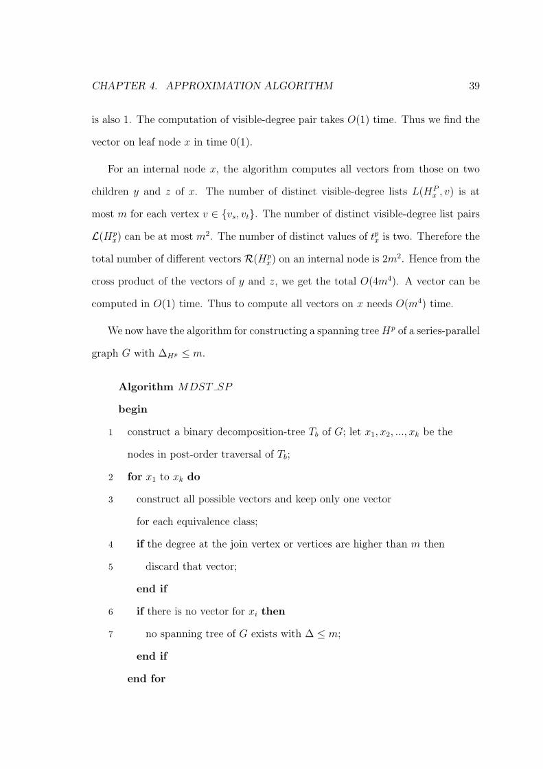
For an internal node x, the algorithm computes all vectors from those on two
children y and z of x. The number of distinct visible-degree lists L(HPx , v) is at
most m for each vertex v ∈ {vs, vt}. The number of distinct visible-degree list pairs
L(Hpx) can be at most m2. The number of distinct values of tpx is two. Therefore the
total number of different vectors R(Hpx) on an internal node is 2m2. Hence from the
cross product of the vectors of y and z, we get the total O(4m4). A vector can be
computed in O(1) time. Thus to compute all vectors on x needs O(m4) time.
We now have the algorithm for constructing a spanning tree Hp of a series-parallel
graph G with ∆Hp ≤ m.
Algorithm MDST SP
begin
1 construct a binary decomposition-tree Tb of G; let x1, x2, ..., xk be the
nodes in post-order traversal of Tb;
2 for x1 to xk do
3 construct all possible vectors and keep only one vector
for each equivalence class;
4 if the degree at the join vertex or vertices are higher than m then
5 discard that vector;
end if
6 if there is no vector for xi then
7 no spanning tree of G exists with ∆ ≤ m;
end if
end for
CHAPTER 4. APPROXIMATION ALGORITHM 40
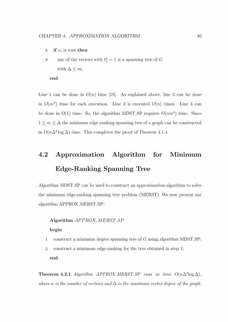
8 if xi is root then
9 any of the vectors with tpx = 1 is a spanning tree of G
with ∆ ≤ m;
end.
Line 1 can be done in O(n) time [19]. As explained above, line 3 can be done
in O(m4) time for each execution. Line 3 is executed O(n) times. Line 4 can
be done in O(1) time. So, the algorithm MDST SP requires O(nm4) time. Since
1 ≤ m ≤ ∆ the minimum edge ranking spanning tree of a graph can be constructed
in O(n∆4 log ∆) time. This completes the proof of Theorem 4.1.4.
4.2 Approximation Algorithm for Minimum
Edge-Ranking Spanning Tree
Algorithm MDST SP can be used to construct an approximation algorithm to solve
the minimum edge-ranking spanning tree problem (MERST). We now present our
algorithm APPROX MERST SP:
Algorithm APPROX MERST SP
begin
1 construct a minimum degree spanning tree of G using algorithm MDST SP;
2 construct a minimum edge-ranking for the tree obtained in step 1;
end.
Theorem 4.2.1 Algorithm APPROX MERST SP runs in time O(n∆4log ∆),
where n is the number of vertices and ∆ is the maximum vertex degree of the graph.
CHAPTER 4. APPROXIMATION ALGORITHM 41
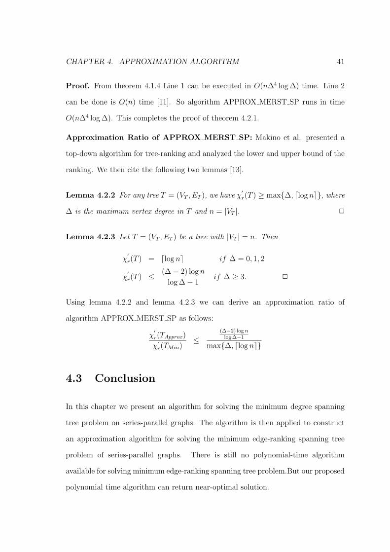
Proof. From theorem 4.1.4 Line 1 can be executed in O(n∆4 log ∆) time. Line 2
can be done is O(n) time [11]. So algorithm APPROX MERST SP runs in time
O(n∆4 log ∆). This completes the proof of theorem 4.2.1.
Approximation Ratio of APPROX MERST SP: Makino et al. presented a
top-down algorithm for tree-ranking and analyzed the lower and upper bound of the
ranking. We then cite the following two lemmas [13].
Lemma 4.2.2 For any tree T = (VT , ET ), we have χ′r(T ) ≥ max{∆, dlog ne}, where
∆ is the maximum vertex degree in T and n = |VT |. 2
Lemma 4.2.3 Let T = (VT , ET ) be a tree with |VT | = n. Then
χ′r(T ) = dlog ne if ∆ = 0, 1, 2
χ′r(T ) ≤ (∆− 2) log n
log ∆− 1if ∆ ≥ 3. 2
Using lemma 4.2.2 and lemma 4.2.3 we can derive an approximation ratio of
algorithm APPROX MERST SP as follows:
χ′r(TApprox)
χ′r(TMin)≤
(∆−2) log nlog ∆−1
max{∆, dlog ne}
4.3 Conclusion
In this chapter we present an algorithm for solving the minimum degree spanning
tree problem on series-parallel graphs. The algorithm is then applied to construct
an approximation algorithm for solving the minimum edge-ranking spanning tree
problem of series-parallel graphs. There is still no polynomial-time algorithm
available for solving minimum edge-ranking spanning tree problem.But our proposed
polynomial time algorithm can return near-optimal solution.
CHAPTER 4. APPROXIMATION ALGORITHM 42
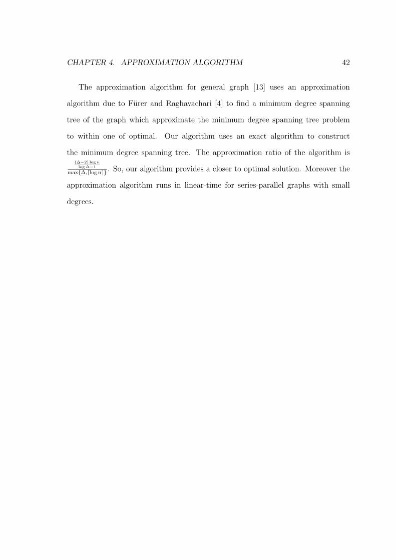
The approximation algorithm for general graph [13] uses an approximation
algorithm due to Furer and Raghavachari [4] to find a minimum degree spanning
tree of the graph which approximate the minimum degree spanning tree problem
to within one of optimal. Our algorithm uses an exact algorithm to construct
the minimum degree spanning tree. The approximation ratio of the algorithm is(∆−2) log n
log ∆−1
max{∆,dlog ne} . So, our algorithm provides a closer to optimal solution. Moreover the
approximation algorithm runs in linear-time for series-parallel graphs with small
degrees.
Chapter 5
Conclusion
In this thesis, we deal with the problem of finding the minimum edge-ranking
spanning tree of series-parallel graphs. We present a polynomial-time optimal
algorithm to find the minimum edge-ranking spanning tree of series-parallel graphs
with small degrees. We also present a polynomial-time optimal algorithm for
finding the minimum degree spanning tree of series-parallel graphs. The algorithm
for minimum degree spanning tree is then used to construct a polynomial time
approximation for minimum edge-ranking spanning tree with an approximation ratio
of(∆−2) log n
log ∆−1
max{∆,dlog ne} , where ∆ is the maximum vertex degree in G and n is the number
of vertices in G. The approximation algorithm runs in linear-time for series parallel
graphs with small degrees. This is the first time that an algorithm is proposed for
solving minimum edge-ranking spanning tree problem on series-parallel graphs.
The approximation algorithm for general graph [13] uses an approximation
algorithm due to Furer and Raghavachari [4] to find a minimum degree spanning
tree of the graph which approximate the minimum degree spanning tree problem
to within one of optimal. Our algorithm uses an exact algorithm to construct the
43
CHAPTER 5. CONCLUSION 44
minimum degree spanning tree. So, our algorithm provides a closer to optimal
solution.
In Chapter 1, we focus on the background history and related motivations on
this research field. We also define our problem and discuss our motivations behind
solving the problem. In Section 1.1, we discuss the historical background and results
on graph coloring and graph-ranking problem. Section 1.2 represents the some
applications of the minimum edge-ranking spanning tree problem and Section 1.3
deals with the scope of this thesis.
In Chapter 2, we discuss the required definitions for solving the problem and
developing the properties. In this chapter we also mention different types of
characterization, which are needed in the way of evolution. In Section 2.1, we
start by giving the definitions of some basic terms of graph which are related
to and used through out this thesis. Section 2.2 defines a special type of graph,
series-parallel graph. It also introduces different properties of a series-parallel graph
and representation of series-parallel graph through the binary decomposition tree.
Section 2.3 presents the upper and lower bound of edge-ranking of trees. Section
2.4 discusses complexity classes of the algorithm. Finally in Section 2.5 we define
approximation algorithm and the approximation ratio.
In Chapter 3, we design an algorithm for finding a minimum edge-ranking
spanning tree of a series-parallel graph. In Section 3.1 we develop the idea of
the equivalence class used in the algorithm. We also proved the validity of the
equivalence class considered. Equivalence classes are key to the solution in dynamic
programming. An appropriate equivalence class reduces the table size required
efficiently. In section 3.2 we discuss the algorithm and analyze its time complexity.
Finally, section 3.3 summarizes the chapter.
CHAPTER 5. CONCLUSION 45
In Chapter 4, we present an approximation algorithm for solving the minimum
edge-ranking spanning tree problem on a series-parallel graph. The algorithm uses
an optimal algorithm to construct a minimum degree spanning tree of the series-
parallel graph, which it then ranks. Section 4.1 presents the algorithm for finding
the minimum degree spanning tree, and its complexity analysis. In Section 4.2 we
provide the approximation algorithm for the minimum edge-ranking spanning tree
problem. We also discuss its time complexity and calculate the approximation ratio
of our proposed algorithm.
We solved the minimum edge-ranking spanning tree problem using dynamic
programming based on the binary decomposition tree. We also use a minimum
degree spanning tree to construct an approximate solution to the problem. The
following problems related to the algorithm for solving the minimum edge-ranking
spanning tree problem of series-parallel graphs are still open.
1. Identify the complexity class of the minimum edge-ranking spanning tree
problem. It is very likely to be in NP-Complete.
2. Reduce the time complexity of the optimal algorithm for solving the minimum
edge-ranking spanning tree on general series-parallel graphs.
3. Develop a linear time approximation algorithm for solving the minimum
edge-ranking spanning tree problem on series-parallel graphs with better
approximation ratio.
4. Develop an approximation algorithm for solving the minimum edge-ranking
spanning tree problem on partial k-trees.
Bibliography
[1] H. Bodlaender, J.R. Gibert, H. Hafsteinsson, T. Kloks, D. Kratsch, H. Muller, and
Z. Tuza, Rankings of graph, SIAM J. Discrete Mathematics, 11 (1998) pp. 168-181.
[2] J.S. Deogun, T. Kloks, D. Kratsch, and H. Muller, On the vertex ranking problem
for trapezoid, circular-arc and other graphs, Discrete Applied Math, 98 (1999) pp.
39-63.
[3] M. Furer, and B. Raghavachari, Approximating the minimum degree spanning tree
to within one from the optimal degree, Proc. of 3rd ACM-SIAM Symp. on Disc.
Algorithms (SODA), pp. 317-324, 1992.
[4] M. Furer, and B. Raghavachari, Approximating the minimum-degree Steiner tree to
within one of optimal, J. Algorithms, 17 (1994) pp. 409-423.
[5] B. Gavish, Topological design of centralized computer networks formulations and
algorithms, Networks, 12 (1982) pp. 355-377.
[6] A.V. Iyer, H.D. Ratliff, and G. Vijayan, Optimal node ranking of trees, Information
Processing Letters, 28 (1988) pp. 225-229.
[7] M. A. Kashem, M. E. Haque, Edge-ranking problem is NP-complete for series-parallel
graphs, Proc. of the 4th International Conference on Computer and Information
Technology (ICCIT), (2001) pp.108-112.
46
BIBLIOGRAPHY 47
[8] M.A. Kashem, X. Zhou, and T. Nishizeki, Algorithms for genmerelized vertex-
rankings of partial k -trees,Theoretical Computer Science, 24 (2000) pp. 407-427.
[9] M. A. Kashem, X. Zhou, and T. Nishizeki, Algorithms for generalized edge-rankings
of partial k-trees with bounded maximum degree, Proceedings of the 1st International
Conference on Computer and Information Technology (ICCIT), pp.45-51, 1998.
[10] R. Krishnan, and B. Raghavachari, The Directed Minimum-Degree Spanning Tree
Problem, Proceedings of the 21st Conference on Foundations of Software Technology
and Theoretical Computer Science, pp. 232-243, 2001.
[11] T.M. Lam and F.L. Yue, Edge-ranking of graphs is hard, Discrete Applied
Mathematics, 85 (1998) pp. 71-86.
[12] T.M. Lam and F.L. Yue, Optimal edge-ranking of trees in linear time, Proc. of the
Ninth Annual ACM-SIAM Symposium on Discrete Algorithms, pp. 436-445, 1998.
[13] K. Makino, Y. Uno, T. Ibaraki, On minimum edge-ranking spanning trees, Journal
of Algorithms, 38 (2001) pp. 411-437.
[14] K. Makino, Y, Uno, T. Ibaraki, Minimum edge ranking spanning trees of threshold
graphs,LNCS, 2518 (2002) pp. 428-440.
[15] K. Miyata, S. Masuyama, S. Nakayama, and L. Zhao, NP-hardness proof and
approximation algorithm for the minimum vertex-ranking spanning tree problem,
Submission for Discrete Applied Mathematics.
[16] S. Nakayama, and S. Masuyama, An O(n3) time algorithm for obtaining the
minimum vertex-ranking spanning tree on permutation graphs, 4th Japanese-
Hungarian symposium on Discrete mathematics and its application, 2005.
BIBLIOGRAPHY 48
[17] S. Nakayama, and S. Masuyama, An algorithm for solving the minimum vertex-
ranking spanning tree problem on interval graphs, IEICE Trans. Fundamentals, E86-
A No. 5 (2003) pp. 1019-1026.
[18] A.A. Schaffer, Optimal node ranking of trees in linear time, Information Processing
Letters, 33 (1989) pp. 91-96.
[19] K. Takamizawa, T. Nishizeki, and N. Saito, Linear time computability of
combinatorial problems on series-parallel graphs, J. Assoc. Comput. Math., 29 (1982)
pp. 623-641.
[20] X. Zhou, M.A. Kashem, and T. Nishizeki, Generalized edge-rankings of trees, IEICE
Trans. on Fundamentals of Electronics, Communications and Computer Science,
E81-A, 2 (1998) pp. 310-320.
[21] X. Zhou, H. Nagai, and T. Nishizeki, Generalized vertex-rankings of trees,
Information Processing Letters, 56 (1995) pp. 321-328.
Index
G[EH ], 13
G[VH ], 13
T , 15
∆, 13
NP, 20
NP-Complete, 21
NP-hard, 21
P, 20
algorithm, 20
application, 7
approximation algorithm, 22
approximation ratio, 22
APPROX MERST SP, 40
complexity
linear-time, 20
polynomial-time, 20
component, 14
edge-ranking problem, 3
finite, 12
forest, 15
graph
adjacent, 12
connected, 14
degree, 13
disconnected, 14
incident, 12
loop, 12
multigraph, 12
multiple, 12
neighbor, 12
parallel, 12
simple, 12
MDST SP, 39
MERST SP, 32
minimum degree spanning tree problem, 7
minimum edge-ranking spanning tree
problem, 4
minimum edge-ranking spanning tree
problem, 6
subgraph, 13
connected, 14
maximal, 14
tree, 15
49
INDEX 50
binary, 15
child, 15
height, 16
internal, 15
leaf, 15
node, 15
depth, 16
height, 16
level, 16
parent, 15
root, 15
rooted, 15
Spanning tree, 16
subtree, 15
vertex-ranking problem, 5