a hardware architecture for gps/ins-enabled wireless sensor networks

A HARDWARE ARCHITECTURE FOR GPS/INS-ENABLED

WIRELESS SENSOR NETWORKS

by

CHUN TANG

A thesis submitted to the Department of Electrical and Computer Engineering

in conformity with the requirements for

the degree of Master of Applied Science

Queen’s University

Kingston, Ontario, Canada

(December, 2011)

Copyright ©Chun Tang, 2011

ii

Abstract

Wireless sensor network technology has now been widely adopted. In many applications, distributed

sensor nodes collect data at different locations and the location information of each node is required.

The Global Positioning System is commonly used to identify the location of the nodes in such

networks. Although GPS localization has consistent long-term accuracy, it is limited by the inherent

dependency on a direct line of sight to 4 or more external satellites. The increasing demand for an

embedded system providing reliable navigation solutions regardless of its operational environment

has motivated investigations into the use of integrated systems that combine inertial sensors with GPS

receivers.

This research proposes a hardware architecture for location-based wireless sensor networks. In

this architecture, each sensor node consists of a GPS receiver, a reduced set of low cost micro-electro-

mechanical-system-based INS and a wireless transceiver. Sensor nodes in WSN are often equipped

with irreplaceable batteries, which makes the power consumption crucial. To reduce the energy

consumption, a microcontroller is used to control the power supply. Besides, a motion detection

scheme is proposed by taking advantage of the ultra low-power wake-up function of the

microcontroller. A low-power featured digital signal processor is used to accomplish the navigation

computation using the Kalman filter for GPS/INS data fusion. Non-Holonomic Constraints derived

velocity updates are applied to reduce the position errors. Field tests are conducted to verify the real-

time performance of the proposed system with a positioning update rate of 20 Hz.

The first test shows that the 2D INS/GPS integration can maintain the average system position

error within 5 meters during a 60-second GPS outage. The second test used low cost inertial sensors.

The average position error was 10.17 meters during a 20-second outage. The largest RMS value of

position errors among these outages was within 14.5 meters. Furthermore, additional accuracy

improvements of approximately 1.4 meters were achieved by utilizing NHC during GPS outages. The

iii

third test shows that the average error during a 30-second outage is approximately 20.6 meters for the

on-foot scenario and 26.7 meters for the in-vehicle scenario.

iv

Acknowledgements

Firstly, I would like to express my deepest gratitude to my supervisor, Dr. Mohamed Ibnkahla, for his

guidance, support and encouragement. Dr. Ibnkahla’s knowledge and insight were invaluable

resources to me throughout my graduate studies. I would also like to thank Dr. Aboelmagd Noureldin

for his unconditional support and invaluable advice. Also, a sincere thank you to Zhi Shen, Walid

Farid Abd El Fatah and Tashfeen Karamat for their patient explanations, discussion, and for

familiarizing me with the navigation devices in their laboratory. I would especially like to

acknowledge Walid for providing the dataset for the first field test in this thesis work.

I would like to extend my thanks to the members of Wireless Sensor Network and

Communication Laboratory: Basel Nabulsi, Abdallah AlMaaitah, Amr El Mougy, Peng Hu, Gayathri

Vijay, Ala Abu Alkheir, Zouheir El-Jabi and Xiao Zhao. They always provided me with the help and

suggestions I needed. Their support made it possible for me to complete this work.

Finally and most importantly, I would like to thank my parents for their unconditional love and

care. This work would not have been possible without their support.

v

Table of Contents

Abstract ................................................................................................................................................. ii

Acknowledgements .............................................................................................................................. iv

Table of Contents ................................................................................................................................. v

List of Figures ..................................................................................................................................... vii

List of Tables ....................................................................................................................................... ix

List of Abbreviations ............................................................................................................................ x

Chapter 1 Introduction ........................................................................................................................ 1

1.1 Background .................................................................................................................................. 1

1.2 Literature Review ......................................................................................................................... 3

1.3 Thesis Objectives and Contributions ............................................................................................ 4

1.4 Thesis Outline .............................................................................................................................. 5

Chapter 2 WSN and Navigation System Overview ........................................................................... 7

2.1 Overview of WSN and ZigBee .................................................................................................... 8

2.2 Overview of the Global Positioning System .............................................................................. 11

2.3 Overview of the Inertial Navigation System .............................................................................. 12

2.3.1 Mechanization and Quaternion Transformation ..................................................................... 13

2.3.2 Estimation Theory and the Kalman Filter ............................................................................... 17

2.3.3 GPS/INS Integration Techniques ............................................................................................ 22

Chapter 3 Accuracy Improvement Methods for Low Cost Systems ............................................. 26

3.1 INS Error Sources and Properties .............................................................................................. 26

3.1.1 Sensor Bias .............................................................................................................................. 27

3.1.2 Scale Factors ........................................................................................................................... 28

3.1.3 Non-Orthogonalities ................................................................................................................ 28

3.2 Inertial Sensor Calibration ......................................................................................................... 29

3.2.1 Six-Position Static Test ........................................................................................................... 29

3.3 Stochastic Sensor Error Modeling .............................................................................................. 31

3.4 Non-Holonomic Constraints ...................................................................................................... 35

Chapter 4 Hardware and Software Implementation ...................................................................... 38

vi

4.1 Hardware Implementation .......................................................................................................... 38

4.1.2 Navigation Data Processing .................................................................................................... 39

4.1.3 RF Transceiver ........................................................................................................................ 40

4.1.4 Power Supply of the Navigation Board ................................................................................... 41

4.1.5 Connectors/Jumpers on Navigation Board .............................................................................. 42

4.1.6 Reset and Wakeup Circuits ..................................................................................................... 43

4.2 Development Tools .................................................................................................................... 44

4.2.1 IAR Embedded Workbench for 8051 ...................................................................................... 44

4.2.2 Code Composer Studio ............................................................................................................ 44

4.3 System Flow ............................................................................................................................... 45

4.3.1 Program Flow of System Initialization ................................................................................... 45

4.3.2 Power Management Scheme ................................................................................................... 48

4.3.3 DSP Memory Allocation ......................................................................................................... 53

4.3.4 Zigbee Node Software Design ................................................................................................ 55

Chapter 5 Tests and Results .............................................................................................................. 60

5.1 Equipment and Setup ................................................................................................................. 60

5.2 Real-Time Performance Analysis .............................................................................................. 61

5.3 Navigation Board Calibration .................................................................................................... 62

5.3.1 Test Setup ................................................................................................................................ 62

5.3.2 Multi-Position Static Test Results ........................................................................................... 63

5.3.3 Random Error Modeling ......................................................................................................... 64

5.4 Open Field Tests ........................................................................................................................ 68

5.4.1 Field Test I .............................................................................................................................. 69

5.4.2 Field Test II ............................................................................................................................. 75

5.4.3 Field Test III ............................................................................................................................ 82

5.5 Summary .................................................................................................................................... 89

Chapter 6 Summary, Conclusions and Recommendations ............................................................ 91

6.1 Summary of Conclusions ........................................................................................................... 91

6.2 Developed Programs .................................................................................................................. 93

6.3 Recommendations for Future Work ........................................................................................... 94

Bibliography ....................................................................................................................................... 96

Appendix A Schematics of the Navigation Board ........................................................................... 99

vii

List of Figures

Figure 2.1 The architecture of the proposed system. ............................................................................. 7

Figure 2.2 Diagram of ZigBee structure. ............................................................................................. 10

Figure 2.3 The architecture of a typical wireless sensor network. ....................................................... 10

Figure 2.4 Illustration of GPS constellation. ........................................................................................ 12

Figure 2.5 l-frame mechanization flow algorithm. .............................................................................. 15

Figure 2.6 A complete picture of the two-step Kalman filter operations. ............................................ 21

Figure 2.7 Loosely coupled GPS/INS integration. ............................................................................... 24

Figure 2.8 Tightly coupled GPS/INS integration. ................................................................................ 25

Figure 3.1 Autocorrelation function of the GM process. ..................................................................... 33

Figure 3.2 Shaping filter of the 1st order GM process. ......................................................................... 34

Figure 4.1 Layout of the navigation board. .......................................................................................... 39

Figure 4.2 PCB layout of the proposed system. ................................................................................... 39

Figure 4.4 Design of the power circuit. ................................................................................................ 42

Figure 4.5 Power control design with a 2-pin jumper and a bipolar junction transistor. ..................... 43

Figure 4.6 DSP initialization routine and DSP reset ISR. .................................................................... 47

Figure 4.7 Flow chart for UART receive ISR. ..................................................................................... 48

Figure 4.8 flow chart for motion detection. ......................................................................................... 50

Figure 4.9 Program flows of DSP_Sleep and Wakeup_ISR. ............................................................... 52

Figure 4.10 Software flow of the whole system. .................................................................................. 53

Figure 4.11 The structure of a typical ZigBee sensor network ............................................................ 56

Figure 4.12 The initialization and configuration of the sink node program flow. ............................... 57

Figure 4.13 The event processing flow of the sink node task event handler. ...................................... 58

Figure 4.14 The event processing flow of the sensor node task event handler. ................................... 59

Figure 5.1 A typical time frame within one second of DSP computation. ........................................... 62

Figure 5.2 The autocorrelation of x-axis accelerometer reading of 2-hour stationary dataset after

removing the bias offset. ...................................................................................................................... 65

Figure 5.3 Magnified view of Figure 5.2. ............................................................................................ 66

Figure 5.4 Correlation time of X-axis accelerometer ........................................................................ 66

Figure 5.5 The autocorrelation of y-axis accelerometer reading of 2-hour stationary dataset after


Figure 5.6 Correlation time of Y-axis accelerometer ........................................................................ 67

viii

Figure 5.7 The autocorrelation of z-axis gyroscope reading of 2-hour stationary dataset after


Figure 5.8 Field test I: Reference trajectory and KF trajectory with 4 simulated GPS outages. ......... 72

Figure 5.9 Field test I: North/East position errors. ............................................................................... 72

Figure 5.10 Field test I: Reference north velocity and KF north velocity. ........................................... 73

Figure 5.11 Field test I: Reference east velocity and KF east velocity. ............................................... 73

Figure 5.12 Field test I: East/North velocity errors. ............................................................................. 74

Figure 5.13 Field test I: Reference yaw and KF yaw. .......................................................................... 74

Figure 5.14 Field test II: GPS trajectory and KF trajectories with 4 simulated GPS outages. ............ 77

Figure 5.15 Field test II: North position errors. ................................................................................... 77

Figure 5.16 Field test II: East position errors. ...................................................................................... 78

Figure 5.17 Field test II: GPS north velocity and KF north velocity. .................................................. 78

Figure 5.18 Field test II: GPS east velocity and KF east velocity. ...................................................... 79

Figure 5.19 Field test II: north velocity errors. .................................................................................... 79

Figure 5.20 Field test II: east velocity errors. ...................................................................................... 80

Figure 5.21 Field test II: GPS yaw and KF yaw. ................................................................................. 80

Figure 5.22 Equipment setup for the field test. .................................................................................... 83

Figure 5.23 Test III.1: GPS trajectory and on-foot Trajectory with 6 GPS outages. ........................... 85

Figure 5.24 Test III.2: GPS trajectory and on-foot trajectory with 5 GPS outages. ............................ 85

Figure 5.25 Test III.3: GPS trajectory and on-foot trajectory with 5 GPS outages. ............................ 86

Figure 5.26 Test III.4: GPS trajectory and in-vehicle trajectory with 5 GPS outages. ........................ 86



ix

List of Tables

Table 4.1 Reset source select of the three position jumper. ................................................................. 44

Table 4.2 Definitions for interrupt vectors. .......................................................................................... 46

Table 4.3 DSP computation accuracy compared with matlab.............................................................. 54

Table 4.4 Memory map report generated from CCS. ........................................................................... 55

Table 5.1 Specifications for ADXL335 and LISY300AL. .................................................................. 61

Table 5.2 Execution time for the Program. .......................................................................................... 62

Table 5.3 Normal gravity constants. .................................................................................................... 63

Table 5.4 Parameters used in accelerometer’s deterministic errors. .................................................... 64

Table 5.5 First order GM model parameters used in field test II. ........................................................ 65

Table 5.6 Specifications for XBow IMU300CC-100. .......................................................................... 69

Table 5.7 GPS/IMU specifications of the reference system. ............................................................... 70

Table 5.8 Field test I: Position/Velocity errors during GPS outages. .................................................. 75

Table 5.9 Field test II: Position/Velocity errors during GPS outages. ................................................. 81

Table 5.10 The accuracy improvement with NHC. ............................................................................. 82

Table 5.11 Specifications for ADIS16003, ADIS16060 and HMC6352. ............................................ 84

Table 5.12 On-foot field test: Position errors during GPS outages. ..................................................... 88

Table 5.13 In-vehicle field test: Position errors during GPS outages. ................................................. 89

x

List of Abbreviations

2D Two-Dimensional

3D Three-Dimensional

ADC Analog-to-Digital Converter

API Application Programming Interface

AR Auto-Regressive

ASCII American Standard Code for Information Interchange

BJT Bipolar Junction Transistor

C/A Coarse-Acquisition

CCS Code Composer Studio

CEP Circular Error Probable

COFF Common Object File Format

CPLD Complex Programmable Logic Device

DARAM Dual Access Random Access Memory

DCM Direction Cosine Matrix

DMA Direct Memory Access

DR Dead Reckoning

DSP Digital Signal Processor

ECEF Earth Centered Earth Fixed Frame

ENU East-North-Up

FPGA Field-Programmable Gate Array

GM Gaussian-Markov

GPIO General Purpose Input/Output

GPS Global Positioning System

HAL Hardware Abstraction Layer

I2C Inter-Integrated Circuit

IAE Innovation-based Adaptive Estimation

xi

IDE Integrated Development Environment

IEEE Institute of Electrical and Electronics Engineers

IMU Inertial Measurement Unit

ISR Interrupt Service Routine

JTAG Joint Test Action Group

KF Kalman Filter

MAC Media Access Control

MCU Micro-Controller Unit

MEMS Micro-Electro-Mechanical Systems

MMAE Multiple-model-based Adaptive Estimation

NED North-East-Down

NHC Non-Holonomic Constraints

NMEA National Marine Electronics Association

OSAL Operating System Abstraction Layer

PAN Personal Area Network

PER Packet Error Rate

PLL Phase-Locked Loop

PPM Parts Per Million

PRN Pseudo-Random Noise

PSD Power Spectral Density

RF Radio Frequency

RSSI Received Signal Strength Indicator

SARAM Single Access Random Access Memory

SFR Special Function Register

SINS Strap-down Inertial Navigation System

SPI Serial Peripheral Interface

SSM State Space Model

xii

UART Universal Asynchronous Receiver/Transmitter

UKF Unscented Kalman Filter

ZDO Zigbee Device Object

1

Chapter 1

Introduction

1.1 Background

The location information is usually important in wireless sensor networks (WSN). It is not only

required by specific WSN applications such as environment monitoring applications, but also used to

improve the routing of WSN, in particular by forwarding the control messages only to a portion of the

network and avoid to waste energy on the nodes that do not contain the route to the destination node.

A typical example is the Location-Aided Routing (LAR) protocol that utilizes location information to

decrease overhead of route discovery [1]. Many other routing protocols such as GeRAF, GeoAODV

and LACBER etc. are also based on the geographical location of the nodes [2-4].

The Global Positioning System (GPS) is usually used to identify the spatial coordinates of a

sensor node in a WSN. Generally, GPS requires direct Line-Of-Sight (LOS) signals from at least four

satellites to figure out where the receiver is. Therefore, a stand-alone GPS may often suffer from

signal blockages in degraded signal environments, such as indoor environments, urban canyons,

foliated areas, etc. The integration of a Strap-down Inertial Navigation System (SINS) with the

Global Positioning System (GPS) has been extensively studied and deployed in different applications.

In these integrated systems, SINS provides position, velocity and orientation information at very high

data rates (usually above 50 Hz) and provides accurate outputs in a short term. However, its

performance deteriorates with time quickly. Therefore, GPS and SINS are complementary. Each

2

system compensates for the other’s drawbacks and it is an efficient way to integrate GPS with SINS

for continuously getting reliable navigation information.

Standard Inertial Navigation Systems use high cost accelerometers and gyroscopes to provide

precise navigation information, which lessens their popularity in general user-end devices. With the

advancement of Micro Electro Mechanical System (MEMS) technology, low-cost MEMS inertial

sensors provide a more affordable solution for GPS/INS integrated navigation systems [5]-[6].

Although MEMS sensors make the navigation system less expensive, more compact and more power

efficient, the performance is relatively poor due to its high instrument bias and drift, its vulnerability

to temperature effects, etc. As a result, the INS errors accumulate rapidly in just a short time interval

unless there are updates from external navigation measurements. These errors can be usually reduced

through robust integration algorithms with regular updates that ensure an acceptable level of

accuracy. A typical example of this is the Kalman filter.

The Kalman Filter (KF), which is named after Rudolf E. Kalman, is commonly used to perform

the GPS/INS data fusion in various applications [7-9]. However, the Kalman Filter has some

drawbacks. Since it is the optimal filter for modeled processes, predefined system dynamic models

are required. If the input data does not fit those models, the positioning accuracy will be significantly

degraded [10]; another major problem with KF is the observability of some of its error states;

moreover, the performance of the Kalman Filter is poor if the sensor noise level is high [11].

Although some alternative algorithms for INS/GPS integration have been investigated and proved

efficient in navigation applications (e.g. Artificial Neural Networks [12]), KF is still computationally

3

efficient, and particularly suitable for real-time applications. Therefore, we use KF as the navigation

algorithm to fuse the data outputs from the GPS and inertial sensors.

1.2 Literature Review

Recently, research efforts have been focused on GPS/INS integration techniques implemented on

real-time embedded systems in which the navigation computation is strictly limited by time without

any post-processing aid. In real-time applications, inertial sensors based on MEMS technology play

an essential part to make the whole system cost-effective and compact.

A Micro-miniature Inertial Measurement Unit (MIMU) and GPS-based integration system has

been proposed by [13]. This system is based on a PC/104 embedded microcomputer and the MIMU

module is composed of three MEMS gyroscopes and three MEMS accelerometers. Six inertial sensor

signals are processed by a multiplexer-based ADC on a customized data acquisition board. The

Micro-programming Controlled Direct Memory Access (MCDMA) technique is introduced to

improve real-time data calculation and achieve fast data exchange.

Qu et al. [14], have described a miniaturized/low-cost navigation system in which a Digital

Signal Processor (DSP) and a Complex Programmable Logic Device (CPLD) are used as a math co-

processor for developing the hardware system. In this proposed system design, CPLD, which has a

fast calculation speed, is mainly used for matrix calculation, whereas DSP is used to control and

schedule the entire system.

V. Agarwal, H. Arya and S. Bhaktavatsala [15], in their paper describe development of a

compact and low-power GPS/INS system based on a FPGA and a floating point DSP. In this paper,

4

they used the FPGA to construct an efficient interface for GPS data acquisition. An internal Dual Port

Random Access Memory (DPRAM) within FPGA was used for asynchronous data transmission

between the GPS and DSP, which significantly reduced the GPS processing overhead on the

navigation processor. It adopted a 16 bit, 250 kHz ADC (ADS8364, Texas Instruments [16]) for

sampling all the analog signals from inertial sensors simultaneously, rather than using an ADC

multiplexer to sample the channels at different time instants.

1.3 Thesis Objectives and Contributions

The primary objective of this thesis is to propose an efficient (compact, low-cost, low-power and light

weight) DSP-based real-time navigation system design for sensor nodes in WSN where cost, size and

power are focal concerns.

During the course of this work, the following tasks were investigated and carried out:

Propose a novel architecture for WSN by using GPS/INS integrated system that enables efficient

navigation/localization under signal degraded environment.

Implement the proposed system design in hardware and optimize it for low-cost, low-power and

compact requirements.

Develop an external-interrupt triggered power management scheme based on the ultra-low-power

wake-up function of a microcontroller to minimize the system power consumption.

Verify the system performance through open area field tests with simulated as well as actual GPS

outages for evaluation of prediction accuracy.

5

1.4 Thesis Outline

The remainder of this thesis is organized as follows:

Chapter 2 reviews the characteristics of GPS and INS separately, followed by the GPS/INS

integration techniques. The basic concepts of GPS will first be provided. A review of INS is

described afterwards with a brief introduction of coordinate frame and relevant coordinate

transformation, as well as the mechanization equations that are usually used in inertial data

processing. The Kalman Filter algorithm is also presented.

Chapter 3 discusses various inertial sensor error sources and their properties. A deterministic

error model is derived in matrix form and a standard calibration method is introduced. Next,

stochastic error modeling is discussed and the process model state equation of EKF for the first order

Gauss-Markov (GM) process is derived in matrix form. Additionally, non-holonomic constraints are

also discussed.

Chapter 4 gives an overview of the total integrated system architecture and describes both the

hardware and software implementation details of the navigation board. After a brief system hardware

description, software development tools are introduced followed by the system program flow with

emphasis given to the system power management scheme.

In Chapter 5, static calibration and random error modeling in the laboratory are carried out and

the results are analyzed. Also, the real-time performance analysis using CCS simulator is presented.

Results of field testing in open areas are presented in this chapter as well. The main idea aims to

evaluate the system performance during GPS signal outages. Non-holonomic constraints are applied

in the second field test to compare the positional errors during GPS outages. The experimental work

6

also includes the verification of the proposed navigation board for both the on-foot and in-vehicle

scenarios.

Chapter 6 summarizes the contributions of this thesis and provides suggestions for future

research.

7

Chapter 2

WSN and Navigation System Overview

A new architecture for GPS/INS-enabled WSNs is proposed in this thesis. The sensor node of this

system is featured with miniaturized dimension, improved power efficiency and processing

overheads. There are mainly 5 blocks in the proposed system (Figure 2.1), which will be presented in

details in Chapter 4:

Data Acquisition Components: accelerometer, gyroscope, GPS, magnetic sensor

Data Processing Unit: DSP

Power Management Unit: microcontroller

Wireless transceiver

Power supply

Figure 2.1 The architecture of the proposed system.

8

In the above system architecture, a radio transceiver is equipped to make the system compatible

with wireless sensor networks. A reduce set of MEMS INS, which consists of a 2-axis accelerometer

and a single-axis gyroscope, is used to provide the acceleration and the angular rate required by the

integrated system. GPS continuously provides reliable positional information. The magnetic sensor

measures the heading angle. A single DSP chip is programmed to process GPS data and carry out the

navigation computation. A PIC MCU is used to control the power supply and accomplish the motion

detection (see Section 4.3.2.1). A brief review of WSN, GPS and INS is given by the following

sections.

2.1 Overview of WSN and ZigBee

A wireless sensor network (WSN) consists of a large number of battery-powered and self-organizing

sensor nodes, which are spatially distributed to monitor physical or environmental conditions. Those

sensors can be deployed anywhere, even in inaccessible areas. There are a wide range of WSN

applications such as environment monitoring, landslide detection, smart homes, precision agriculture,

battle surveillance, etc. However, in many applications, the battery equipped on each sensor node is

not replaceable, which makes the power constraint extremely tight.

One of many significant options for WSN is the ZigBee technology. The ZigBee is an open

global standard which is built on top of the IEEE 802.15.4-2003 standard for Wireless Personal Area

Networks (WPANs). The IEEE 802.15.4 standard defines the physical and MAC layers, whereas

ZigBee defines the network and application layers. A typical ZigBee network is a multi-hop network

that enables low power consumption, low cost and low data rate for short-range wireless connections

9

between battery-powered devices[42]. The ZigBee system structure is shown in Figure 2.2. ZigBee

standardizes both the network and the application layer:

Network (NWK) layer

The network layer ensures the proper operation of the MAC layer and provides an interface to the

application layer. This layer establishes the network, as well as discovers nodes, and permits them to

join or leave the network. It supports three different network topologies: star, tree and peer to peer.

Application layer

The APL layer is composed of three sublayers, which are shown in Figure 2.2. Application Support

Sublayer (APS) is mainly responsible for interfacing and controlling devices, address mapping, and

message transmission between devices. The Zigbee Device Object (ZDO) is responsible for defining

the logical type of the device (i.e. ZC, ZR or ZED), and discovering new devices in the network and

identifying their application services. The application framework is at the top of the APL layer, which

provides an execution environment for application objects to send and receive data. The application

objects, which are defined by the manufacturer, implement various applications such as light switch,

heating control or security control, etc.

A typical ZigBee sensor network is composed of sensor nodes, routers and sink nodes. A certain

amount of sensor nodes are geographically distributed and deployed within the maximum RF range of

fixed relay nodes (routers in the network), in self-organized style. After the primary data processing,

the location information of each sensor node will be transmitted through the distributed network with

multi-hop routing. Once the data reach the sink node, they can be sent to the manage node through the

10

Internet and monitored by the terminal user. The architecture of such a wireless sensor network is

shown as Figure 2.3.

Figure 2.2 Diagram of ZigBee structure.

Figure 2.3 The architecture of a typical wireless sensor network.

11

2.2 Overview of the Global Positioning System

Developed by the U.S. Department of Defense (DoD), the Global Positioning System (GPS) is well

known as an all-weather, worldwide, satellite-based radio-navigation system that comprises three

segments: the Space Segment, the Control Segment, and the User Segment. The GPS signal is

broadcasted at two different carrier frequencies: the primary frequency at 1575.42 MHz (L1) and the

secondary frequency at 1227.6 MHz (L2). Signals are encoded using Code Division Multiple Access

(CDMA) so that each signal is distinguishable from others based on its unique spread code for each

satellite. L1 is modulated by two types of Pseudo-Random Noise (PRN) codes: the Coarse-

Acquisition (C/A) code at 1.023 MHz, which is for civilian use, and the Precise (P) code at 10.23

MHz, which is only for military use. L2 is only modulated by the P code.

In general, the current available GPS signal consists of three types of measurements: pseudo-

range (a pseudo-range is an estimate of the distance between the GPS receiver and a navigation

satellite before being error corrected), carrier phase and Doppler measurements. Pseudo-range

measurements are obtained by comparing the PRN codes transmitted from the satellites with the

replica PRN codes generated by the receiver to determine the time shift required for the signal to

propagate from the satellite to the receiver. The reason why it is termed as pseudo-range instead of

range is that the clocks of the satellites and the receiver are not synchronized and the measurements

contain clock biases. Since there are four unknown parameters (three coordinates and the clock bias)

in the system equations, it is necessary to have at least four satellites calculate the receiver position.

Carrier phase measurements are used when a high degree of precision is required in some

applications such as geodetic surveying. The Doppler frequency represents the frequency shift caused

12

by the rate of change of the carrier phase measurements. It can be used to calculate the relative

velocity between the receiver and the satellite. Similar to the case of pseudo-range measurements, the

clock bias is also considered to be an unknown parameter in the velocity calculation. Therefore, at

least four Doppler measurements are necessary to compute the velocity of the receiver.

Figure 2.4 Illustration of GPS constellation.

2.3 Overview of the Inertial Navigation System

An Inertial Navigation System is an autonomous Dead Reckoning (DR) system that usually combines

accelerometers and gyroscopes to provide position and velocity by measuring the accelerations and

angular rates applied to the system’s inertial frame. Other types of DR sensors may also be used in

INS such as the compass, odometer, inclinometer, altimeter, etc. Unlike the GPS that requires

external signals to provide positional information, INS is self-contained and immune to jamming and

deception, regardless of the operational environment. However, the INS measurements are corrupted

by system errors such as inertial alignment errors and sensor errors [17]. Generally there are two

13

types of INS: these are classified by the way their sensor axes fix, and are called the gimbaled and

strap-down systems. The strap-down system is used in this thesis.

The navigation computation process is briefly introduced in the following sections.

2.3.1 Mechanization and Quaternion Transformation

The mechanization equations convert the IMU measurements---specific forces from accelerometers

and angular velocities from gyroscopes---in the body frame into navigation information (position,

velocity and attitude) in the local level frame where the data fusion and navigation calculation are

performed.

The low-cost MEMS sensor suffers from deterministic and stochastic errors that will be

presented in Chapter 3. The sensor errors in the raw measurements need to be compensated before the

mechanization calculation is performed. After eliminating the sensor errors from the raw

measurements, the angular rates in the body frame are integrated to obtain the new orientation of the

INS by updating the rotation matrix from b-frame to local level frame by using the quaternion

approach. The angular rate measurement contains both the rotation generated by the INS and the

Earth rotation. The earth rotation rate should be converted into the b-frame and removed from the

gyro-sensed angular rates. The next step of the IMU data integration is to rotate the specific force

measurement from the body frame to the local level frame. The specific force measurement f is

combined by the gravity g and the INS acceleration a, which is given by:

=a-g (2.1)

14

After removing the gravity component, the INS acceleration is integrated to calculate the INS

velocities and positions in the local level frame.

The l-frame inertial navigation equations can be expressed as follows:

= (2.2)

where，

the dot (.) represents the time derivative,

‘l’ and ‘b’ denote the local level frame and b-frame,

, and is the position vector ( ), velocity vector ( ) and

the gravity vector respectively，

, and h is the geodetic latitude, geodetic longitude and geodetic altitude respectively,

is a skew-symmetric matrix of the INS angular rate and ,

is a skew-symmetric matrix of Earth rotation angular rate e and

,

is the rotation matrix from the b-frame to the l-frame,

and , , and

(2.3)

15

In the above equations, and are measured by 3 gyroscopes

and 3-axis accelerometer respectively. The skew-symmetric matrix corresponding to the vector

is defined as:

(2.4)

The algorithmic flow diagram of the l-frame mechanization is shown in Figure 2.5.

Figure 2.5 l-frame mechanization flow algorithm.

The attitude of a rotating body in the b-frame with respect to a reference frame (i.e. the local

level frame) can be expressed by using different attitude parameterization techniques, such as Euler

angles, quaternion, and DCM. Due to its computational efficiency and simplicity, the quaternion

approach is utilized in this thesis to update the rotation matrix , by integrating the angular

velocities of body rotation measured by gyroscopes.

16

The quaternion q is a vector with four quaternion parameters. Hamilton’s quaternion is defined

as a hyper-complex number, which is represented as follows [18]:

(2.5)

where,

q0, q1, q2, q3 are real numbers,

set [1, i, j, k] forms the vector basis for a quaternion vector space and

.

Quaternion transformation from one coordinate frame to another is only effected by a single

rotation vector Θ [19]:

(2.6)

where , and are three components of the rotation angle and

(2.7)

The definition of the four quaternion components implies that , which

means there are only three independent quaternion parameters and Equation (2.7) can be used to

normalize the quaternion operations.

The relationship between the DCM and the quaternion parameters is represented as follows:

(2.8)

17

and the first-order differential equation for the quaternion components is given by:

(2.9)

where the skew-symmetric matrix and , and are the

angular rates of body rotation.

2.3.2 Estimation Theory and the Kalman Filter

Estimation is a process of estimating a set of values for a set of parameters based on a set of

observations. The mathematical relationship between the observations and the unknown parameters

(the measurement equation) can be expressed as a function of time t:

(2.10)

where,

z(t) is the m-dimensional observation vector,

H(t) is an mxn matrix which is called the system design matrix,

x(t) is the n-dimensional parameter state vector, and

v(t) is the measurement noise.

There is also a process model that describes the parameter dynamics. Similar to Equation (2.10),

the process model is usually expressed as follows:

(2.11)

where,

the dot (.) denotes a time derivative,

18

F(t) is an n x n matrix which is called the system dynamic matrix,

G(t) is the noise shaping matrix which describes how the noise sources are distributed among

the state vector components, and

w(t) is the process driving noise.

The Kalman filter is a recursive state estimator in which the optimal estimate in the least squares

sense of the actual state vector is calculated by a series of prediction and measurement update

processes. As discussed in Section 1.2, the Kalman filter is a common tool to transfer the GPS and

INS measurements into positions, velocities and attitudes. In GPS/INS applications, the inertial

sensor measurements are obtained at discrete points in time, and the parameter state vector is

estimated in discrete time intervals. Therefore, a discrete time adaption of Equation (2.11) is required

as follows:

(2.12)

where,

is the state transition matrix between time and ,

is the parameter state vector at time ,

Similarly, the measurement model of a discrete-time controlled process is expressed as:

(2.13)

In GPS/INS navigation applications, sensor measurements are obtained at discrete times. If we

let be the state vector at those discrete times, then can be obtained in the following form:

Ф (2.14)

19

where Ф is the state transition matrix.

Equation (2.15) is the 9-state vector used in the EKF for navigation computation and Equation

(2.16) shows the corresponding state transition matrix [20]:

(2.15)

Ф (2.16)

where,

, , ,

,

, ,

, ,

.

Equation (2.14) is the discrete-time dynamic model corresponding to the continuous-time model.

Then the covariance matrix of process noise has the form , where is the covariance matrix

of the white noise process w(t):

20

(2.17)

The Kalman filter algorithm is a two-step process, i.e. prediction and update. Figure 2.6 provides

a complete description of the two-step Kalman filter operations.

The optimum combination of measurement and estimated state vector at time k is obtained from:

(2.18)

where,

The hat (^) denotes estimate,

the superscript minus (-) denotes the estimate prior to the measurement at time k,

denotes the Kalman gain,

denotes the a priori estimate, and

represents the measurement vector at time k.

The Kalman filter gain used in the equation is given by:

(2.19)

The covariance matrix of estimation uncertainty is given by:

(2.20)

where, denotes the error covariance matrix prior to using the updated sensor measurements.

21

Figure 2.6 A complete picture of the two-step Kalman filter operations.

To recursively calculate the Kalman gain for time k+1, the predictions for the state estimate

and its associated error covariance matrix at the next step (epoch k+1) are given by:

Ф (2.21)

Ф Ф (2.22)

where, for all k and i.

And, for the error covariance matrix ,

(2.23)

The random process to be estimated can be modeled in the form

Ф (2.24)

And the process measurement can be modeled as a linear function of the state vector while

the statistical properties of the additive noise is given:

(2.25)

22

where,

is the measurement sensitivity matrix (observation matrix) at time k, and

denotes the additive measurement noise which is the electronic noise generated by sensors.

represents the covariance matrix of sensor noise as follows:

(2.26)

2.3.3 GPS/INS Integration Techniques

There are two main integration strategies applied to GPS/INS integration at the software level using

the KF algorithm: loosely coupled integration and tightly coupled integration.

2.3.3.1 Loosely Coupled Integration

With the loosely coupled integration algorithm, the GPS raw measurements (pseudo-range

measurements, carrier phase measurements and Doppler measurements) are first fed to a GPS-only

Kalman filter to calculate the GPS derived positions and velocities before being used as observation

updates to aid the INS for the navigation KF. It is common for the loosely coupled approach to use

the cascaded scheme to combine GPS positions and velocities with INS raw measurements to form

the error residuals. These are then used by the navigation KF to estimate the observable INS errors

such as biases, drifts and misalignment errors. These estimates then feedback to compensate new INS

measurements.

Based on different system requirements, the loosely coupled scheme can either be implemented

in open-loop or closed-loop configurations. Open-loop implementation does not require feedback

from the navigation KF. Therefore, all the IMU measurements and INS-derived navigation

23

information are not corrected before being used. This is a simple configuration which is not well

suited to low-cost MEMS IMU, for the reason that large navigation errors cannot be compensated for

and those errors may degrade the system accuracy quickly without the feedback loop. Based on the

fact that MEMS sensors are not very accurate and their errors fluctuate rapidly, real-time feedback

proves to be particularly useful to enhance the performance of the integrated navigation system.

Compared with the tight integration strategy, the primary advantage of the loosely coupled

integration is that the dimension of the state vectors in the navigation KF is smaller than that in the

tightly coupled case [21]. It takes shorter filter convergence time and has a lower computation load.

Therefore, the loosely coupled integration approach has been widely applied in various applications

due to its flexibility and fast processing time.

The main drawback of loosely coupled integration is that the GPS receiver cannot compute

positions and velocities when the number of tracked GPS satellites is less than four. Therefore, INS

should work in a stand-alone mode under harsh GPS conditions. Another disadvantage is that there

are two independent Kalman filters in the loose integration scheme, which means the process noise is

added to both the GPS Kalman filter and the navigation Kalman filter.

2.3.3.2 Tightly Coupled Integration

Tightly coupled integration is another common strategy used to fuse navigation data provided by the

GPS/INS sensing pair [22-24]. In tight integration strategy, only one single integrated filter is used for

the data fusion. Without the GPS filter, raw GPS measurements are fed to the navigation filter

24

directly, instead of GPS positions and velocities. In this case, the GPS receiver clock bias and drift is

added into the filter error states and used to correct the GPS pseudo-range and Doppler measurements.

Figure 2.7 Loosely coupled GPS/INS integration.

Consequently, the output of this navigation filter can be used to aid the GPS receiver in tracking

satellites.

Clearly, compared with loosely coupled integration, tightly coupled integration is more tolerant

of GPS outages, because it allows for efficient use of GPS pseudo-range measurements when the

number of tracked navigation satellite is less than 4. Moreover, the process noise is only added to a

single Kalman filter, which improves GPS data filtering. However, since the navigation filter needs

an additional component, i.e. GPS pseudo-range measurements, in the system model, the state vector

25

size of tight integration is larger than that of loose integration. It leads to longer convergence time for

error estimates and increased computational loads. Another negative feature of the tight integration

scheme is the indirect GPS measurements which weaken the degree of the observability of the state

vector more than the loose integration strategy.

Figure 2.8 Tightly coupled GPS/INS integration.

26

Chapter 3

Accuracy Improvement Methods for Low Cost Systems

MEMS inertial sensors are small, compact and cost effective, which makes them efficient and

affordable in most civilian navigation applications. The output of MEMS-based IMU is accurate in a

short time period. However, they are significantly affected by various error sources which accumulate

and grow over time, resulting in large position and orientation errors. Hence, it is necessary to

calibrate these errors and remove them from the raw data.

3.1 INS Error Sources and Properties

The error of inertial sensors can be divided into two categories: deterministic errors and stochastic

errors. Deterministic error sources include bias offsets, scale factor instabilities and non-

orthogonalities. These sources are usually determined by specific calibration methods in a laboratory

environment. The stochastic errors include sensor bias drifts and scale factor drifts. In the case of the

gyroscopes, the angular rate measurements given by gyroscope sensors can be described by the true

input angular rate and the error terms in the following equation in which the bias coefficients and the

anisoelastic bias coefficient are neglected and only the first order scale factor is considered [17]:

(3.1)

where,

is the x-axis gyroscope measurement

27

is the true angular rate about x axis,

and are the true angular rate about y axis and z axis respectively,

is the first order x-axis linear scale factor,

and denote the cross-axis coupling coefficients (i.e. non-orthogonalities),

is the x-axis bias offset, and

is the sensor bias drift and white noise.

Similarly the accelerometer error model is given by the following equation:

(3.2)

If is substituted by , based on Equation (3.1), the outputs of a triad of gyroscopes

can be expressed in matrix form as follows:

(3.3)

3.1.1 Sensor Bias

The inertial sensor bias is defined as the average of the inertial sensor output over a specified time,

measured at specified operating conditions that have no correlation with input acceleration or rotation

[25]. Bias of accelerometer is expressed in meters per square second ( ) and bias of gyroscope is

expressed in degrees per hour ( ).

28

There are generally two parts of the sensor bias: the bias offset and the bias drift. The bias offset

is deterministic in nature and stable over a certain period of time if the sensor stays on. The bias offset

is negligible for high-end inertial sensors. However, the bias offset in low-cost MEMS sensors cannot

remain constant over long periods of time and it varies from one start (switch-on) to another. The bias

offset error can be determined by calibration and removed from the raw data. The bias drift refers to

the error which accumulates over time [26]. It is random in nature and should be modeled as a

stochastic process.

3.1.2 Scale Factors

A scale factor is the ratio of a change in the output relative to a change in the input intended to be

measured [25]. According to the definition, it can be acquired as the slope of the straight line which is

given by using the least-square method to the input-output data. The scale factor is typically

expressed in parts per million (PPM). Similar to sensor bias, the scale factor is deterministic in nature

and can be determined by calibration. The scale factor of low-cost IMUs changes from switch-on to

switch-on.

3.1.3 Non-Orthogonalities

Both the accelerometers and gyroscopes in IMUs should be mounted in orthogonal triads. However,

one axis cannot be perfectly orthogonal to the other due to manufacturing errors, so that the

measurement from one axis is correlated to the other axes in the body frame.

29

3.2 Inertial Sensor Calibration

Inertial sensor calibration is a comparison between sensor outputs and reference information to

determine the sensor errors like noises, biases, drifts, scale factors and non-orthogonalities.

3.2.1 Six-Position Static Test

Generally, standard calibration methods were designed for navigation-grade and tactical-grade

inertial sensors in laboratory environments, such as the six-position static test and the angular rate test

[17].

The six position test requires a level table on which the inertial system is installed with its three

accelerometer axes alternately pointing up and down. When one of the sensitive axes is orthogonal to

the level table, the acceleration of gravity is taken as the reference and the specific force measurement

can be given using Equation (3.2) [27]:

(3.4)

(3.5)

where,

and denotes the accelerometer measurement when it points up and down

respectively,

g is the magnitude of the gravity vector, and

b and s are the bias error and first order scale factor of the sensitive axis.

The combination of Equation (3.4) and Equation (3.5) gives:

30

(3.6)

(3.7)

Equation (3.6) and Equation (3.7) can also be used for the static gyroscope test by taking the

earth rotation rate as reference signal. However, consumer-grade gyros such as MEMS gyros

cannot use Equation (3.7) to calculate the scale factor s because the earth rotation rate is completely

masked by MEMS sensor noise.

By using the static six-position method to measure the deterministic errors of accelerometers, the

Equation (3.3) can be rewritten as [27]:

(3.8)

The true input specific forces at six positions are given by:

(3.9)

The average accelerometer measurements (and , etc.) are obtained by

recording the static sensor outputs of a certain time period (at least 15 minutes) when the inertial

system is mounted on the level table with its x-axis pointing down. In this way, the measurement

matrix can be expressed in this form:

(3.10)

31

where and so on.

By using the least squares method, the deterministic error coefficient matrix M can be estimated

as follows:

(3.11)

Analogous to the accelerometer case, this estimation method can be also applied to the

gyroscope calibration by either using the earth rotation rate for high-grade sensors or using a precise

turn table for MEMS sensors. In the later case, the inertial system is fixed on the testing table and

rotates with a constant angular rate that serves as the preset reference value . The test needs to

perform the rotation in both the clockwise and anti-clockwise directions for each sensitive axis. Then

the true input rotating speeds are given by:

(3.12)

3.3 Stochastic Sensor Error Modeling

The stochastic part of the inertial sensor errors generally includes two parts: long-term (low-

frequency) and short-term (high-frequency) components [28]. The high frequency component is

characterized by white noise, whereas the low frequency component consists mainly of correlated

noise. The wavelet de-noising technique is usually used to de-noise the high-frequency component of

32

the inertial sensors prior to processing [29, 30]. In most GPS/INS applications, using white Gaussian

noise to model the low-frequency noise component is not adequate. It is a common way to generate

the colored (correlated) noise by passing a white noise of zero mean through a shaping filter. The

colored noise can be modeled as various random processes such as Auto-Regressive (AR) processes

and Gauss-Markov (GM) processes. In Kalman filter implementations for INS/GPS, a frequently used

method to shape the correlated noise is the first order GM process, which has a simple mathematical

description and fits a large number of physical processes with acceptable accuracy.

A GM process is a stationary Gaussian process which has an exponential autocorrelation. The

autocorrelation function of a GM process X(t) is given as follows:

(3.13)

where,

is the time constant (correlation time), and

is the noise variance of the GM process.

The correlation time 1/ is evaluated at , i.e.:

(3.14)

The power spectral density (PSD) function of a GM process is given by:

(3.15)

or

(3.16)

33

Figure 3.1 Autocorrelation function of the GM process.

Figure 3.1 implies that the correlation between measurement samples becomes weaker as the

time-distance between samples increases.

First order Gauss-Markov (GM) process can be expressed by the following first order differential

equation [31]:

(3.17)

where,

w(t) is a white noise of zero-mean, and

x(t) denotes a time-correlated (or colored) noise modeled by the first order GM process.

The discrete-time form of the 1st order GM process is given by (at sampling interval):

(3.18)

34

Based on Equation (3.18), the shaping filter of the 1st order GM model can be described by

Figure 3.2:

Figure 3.2 Shaping filter of the 1st order GM process.

The first 9 elements of the KF state vector are introduced in Chapter 2. The Kalman filter for the

GM model has 15 error states in total and the additional 6 states consist of 3 accelerometer bias drift

errors and 3 gyroscope bias drift errors, namely, and respectively.

From Equation (3.18), the state space form of the 6 inertial sensor random errors can be

expressed in the following matrix form:

(3.19)

where,

35

(3.20)

After adding the 6 inertial sensor random errors into the error state vector, the state transition

matrix is given as follows:

ФФ

where,

Ф is given by Equation (2.16),

and is given by Equation (2.8).

3.4 Non-Holonomic Constraints

The Non-Holonomic Constraints (NHC) are originally used to improve the navigation accuracy of

land vehicles. The constraints refers to the fact that the vertical velocity and the sideway velocity of a

land vehicle is almost zero unless it jumps off the ground or slides on the ground [32]. Therefore,

there are two non-holonomic constraints in the body frame that can be used as additional

measurement updates to the Kalman filter:

(3.21)

where, and are inertial sensor noises.

36

These two non-holonomic constraints may also fit the motion dynamics of other kinds of

applications such as animal monitoring and pedestrian navigation. To minimize errors when applying

NHC, the IMU should be installed close to the rotational centre of the moving vehicle and the inertial

sensors should be accurately aligned to the b-frame.

By using the non-holonomic constraints, we have two sensor measurements in the body frame,

which are provided by the accelerometers:

(3.22)

and the velocity errors can be expressed by:

(3.23)

where,

and are the velocity error vectors in the b-frame and the l-frame respectively,

is the rotation matrix from l-frame to b-frame,

denotes cross product,

, and

is the attitude error vector, .

The measurement model of non-holonomic constraints can be written as:

(3.24)

where,

x is a 15-state vector of EKF and

.

37

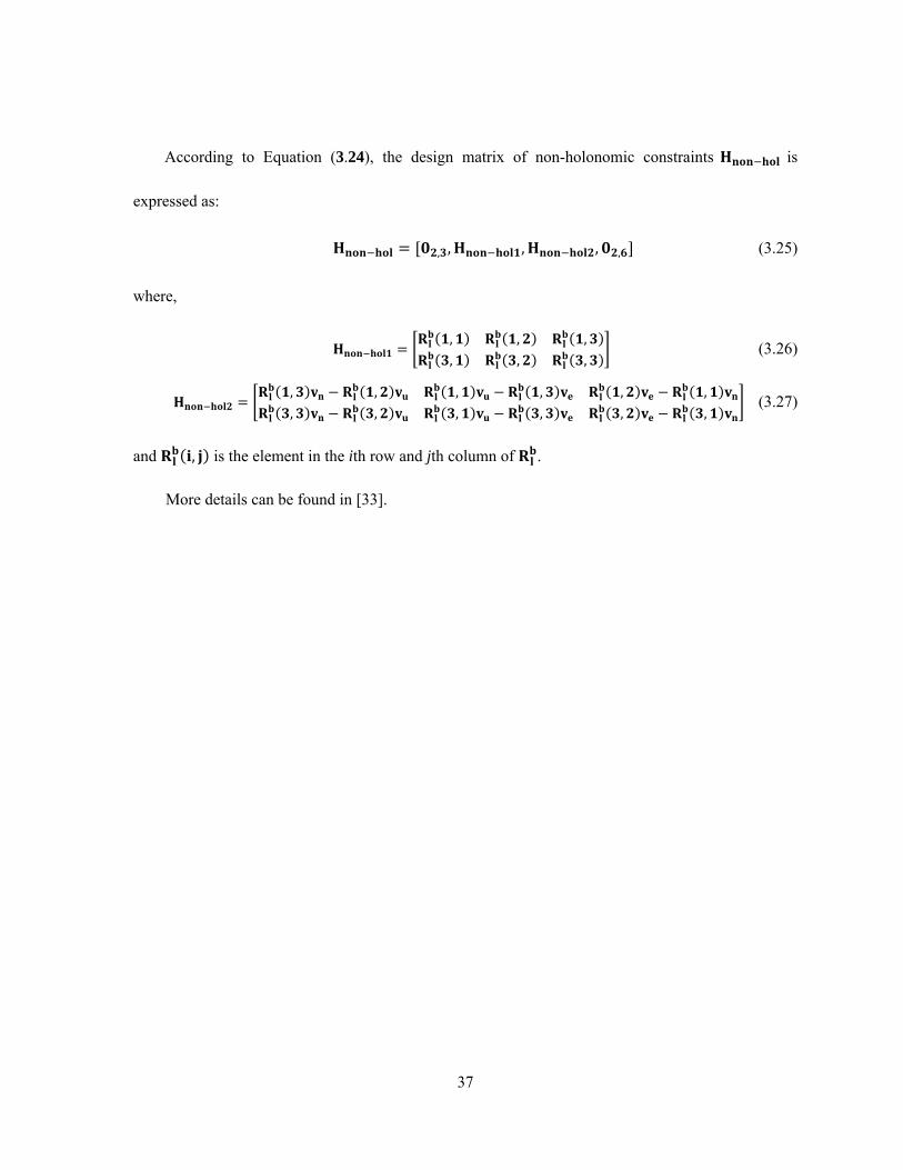
According to Equation (3.24), the design matrix of non-holonomic constraints is

expressed as:

(3.25)

where,

(3.26)

(3.27)

and is the element in the ith row and jth column of .

More details can be found in [33].

38

Chapter 4

Hardware and Software Implementation

4.1 Hardware Implementation

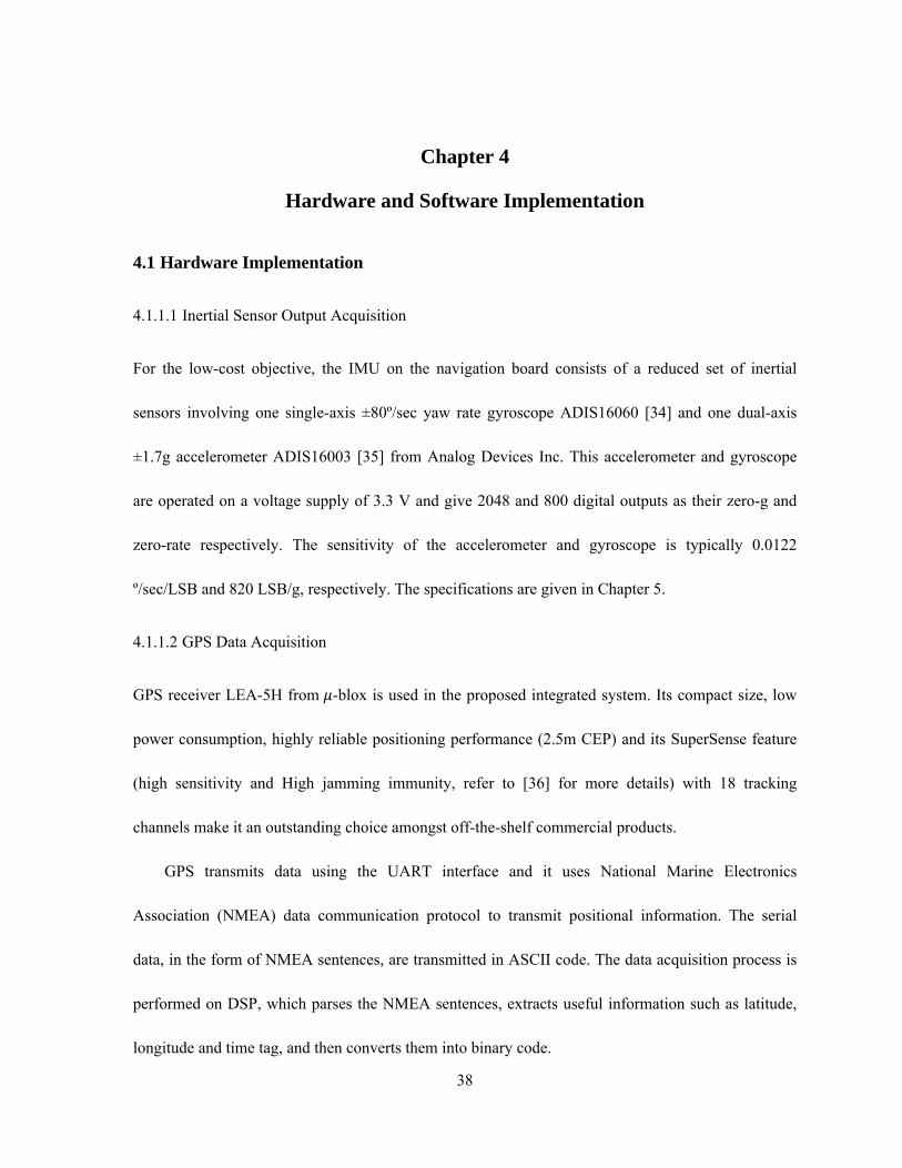
4.1.1.1 Inertial Sensor Output Acquisition

For the low-cost objective, the IMU on the navigation board consists of a reduced set of inertial

sensors involving one single-axis ±80º/sec yaw rate gyroscope ADIS16060 [34] and one dual-axis

±1.7g accelerometer ADIS16003 [35] from Analog Devices Inc. This accelerometer and gyroscope

are operated on a voltage supply of 3.3 V and give 2048 and 800 digital outputs as their zero-g and

zero-rate respectively. The sensitivity of the accelerometer and gyroscope is typically 0.0122

º/sec/LSB and 820 LSB/g, respectively. The specifications are given in Chapter 5.

4.1.1.2 GPS Data Acquisition

GPS receiver LEA-5H from -blox is used in the proposed integrated system. Its compact size, low

power consumption, highly reliable positioning performance (2.5m CEP) and its SuperSense feature

(high sensitivity and High jamming immunity, refer to [36] for more details) with 18 tracking

channels make it an outstanding choice amongst off-the-shelf commercial products.

GPS transmits data using the UART interface and it uses National Marine Electronics

Association (NMEA) data communication protocol to transmit positional information. The serial

data, in the form of NMEA sentences, are transmitted in ASCII code. The data acquisition process is

performed on DSP, which parses the NMEA sentences, extracts useful information such as latitude,

longitude and time tag, and then converts them into binary code.

39

JTAG Interface

CC2430 Interface P 2

PICMCU

Swi-tch

Swi-tch

CC2430 Interface P 1

DSPTMS320VC

5505

LE

D

LE

D

LE

D

LE

D

LE

D

LE

D

LED

Magnetic Sensor

Accelerometer

Gyroscope

Voltage Converters

Mounting HoleMounting Hole

Supply-Voltage Supervisory Circuits

ExternalFlash

Memory PICMCU

Programm-ing

Interface

GPS Interface

Figure 4.1 Layout of the navigation board.

Figure 4.2 PCB layout of the proposed system.

4.1.2 Navigation Data Processing

40

The DSP used for this design is a 196 pin fixed-point TMS320VC5505, which is a member of TI’s

TMS320C5000 family. This DSP is well designed for low-power applications, capable of operating at

a maximum CPU frequency of 100 MHz when the core voltage is 1.3 V.

The DSP clock, which is used by the CPU and most of the peripherals, is controlled by the

system clock generator. The clock generator can either be driven by the 32.768-KHz on-chip real-

time clock (RTC) oscillator or accept an input reference clock from the CLKIN pin. In the present

design, the 32.768-KHz internal oscillator is used to provide the clock signals to both the RTC timer

and the DSP clock generator by setting the CLK_SEL pin low [37]. To generate a system clock signal

as high as 100 MHz, the phase-locked loop (PLL) circuit in the clock generator is programmed to

multiply the input clock 32.768 KHz, by using a 3052x multiplier rate, which is controlled through

the PLL control registers.

To improve the real-time performance and reduce the data acquisition overheads, FPGA is used

in many GPS/INS applications to assist DSP in receiving navigation data. The integration of a FPGA

and a DSP can significantly improve the calculation efficiency since DSP can directly fetch the data

instead of waiting for the low speed serial I/O operation. Although the real-time system may benefit

from FPGA in high sampling data-rate cases, a single-chip DSP can provide comparable performance

when the sampling data rate is low. And most importantly, a single DSP chip makes the navigation

system simpler and more compact, which meets the requirements of energy-sensitive applications and

cost-sensitive applications.

4.1.3 RF Transceiver

41

CC2430 is a System-on-Chip solution from TI that contains a high performance and low power 8051

processor core and 2.4 GHz IEEE 802.15.4 compliant RF transceiver. It is highly suited for systems

that require ultra-low power consumptions. When the microcontroller is running at 32 MHz, the

current consumption of the transmitter/receiver is typically as low as 27 mA. In addition, it features

by four flexible power modes with very short transaction time between low-power modes and active

mode, which can effectively reduce the average power consumption in low duty cycle systems.

To measure the communication range, a range test has been conducted in an open field

environment, with one transmitter placed on the ground and one receiver placed one meter above the

ground. In this test, the transmitter continued to send data packets to the receiver. CC2430 has a built-

in Received Signal Strength Indicator (RSSI) giving a digital value that can be read from one of its

special function registers. The RSSI used in this test was the average RSSI of the last 32 received

packets. The Packet Error Rate (PER) and RSSI are the parameters that are used to determine the

communication quality of this test.

When PER was not increasing, and RSSI was higher than -75 dBm, the communication quality

was considered acceptable. Otherwise, the received signal was regarded as weak and unstable.

Based on the range test, the effective range of the radio link between two CC2430 nodes is

approximately 277 meters, when the transmit power is 19 dBm (with a device current consumption of

32.4 mA [38]), and the wireless transmission is a LOS propagation.

4.1.4 Power Supply of the Navigation Board

42

The power supply set required for the navigation board is [1.3V, 1.8V, 3.3V, 5V]. The 3.3V and 5V

are used by all the peripherals. DSP requires 1.3V and 1.8V for core power and 3.3V for the I/O pins.

Three “AA” size batteries (3 1.5V) are used to provide the DC power, which is initially regulated at

5 V by a fixed-output boost converter TPS61032 [39]. This converter also provides an interrupt signal

(INT0) required by DSP. Then 1.3V, 1.8V and 3.3V power supplies are generated by using three

adjustable low-dropout voltage regulators TPS76601 [40]. The DSP power-up sequence specifically

requires that the core-level supplies (1.3V and 1.8V) must power up before the I/O level supplies

(3.3V). Therefore, the ENABLE signal of the 5V-to-3.3V converter is connected with the

POWERGOOD pin of the 5V-to-1.3V converter through a NPN transistor to guarantee a sufficient

time delay between the core power-up and I/O power-up. More details of the power supply circuit

design can be found in Figure A.4, Appendix A.

Figure 4.3 Design of the power circuit.

4.1.5 Connectors/Jumpers on Navigation Board

43

As shown in Figure 4.1, the navigation board has two 20-pin SMD connection headers for interfacing

with the CC2430EM board. This board is also supplied with a standard 14-pin JTAG header interface

that is used by emulators to interface with DSP and a 5-pin header that is used as the programming

interface of PIC16F886 MCU. There is a 2-pin jumper in parallel with a Bipolar Junction Transistor

(BJT) that is connected with the power supply of each power driven component (i.e. GPS, inertial

sensors, and magnetic sensor) and controlled by the PIC16F886 MCU. These bipolar junction

transistors are used as power-on/off switches and controlled by software. This power management

ability will be disabled when the 2-pin jumpers are connected.

Figure 4.4 Power control design with a 2-pin jumper and a bipolar junction transistor.

4.1.6 Reset and Wakeup Circuits

The reset circuit of DSP is based on the supply-voltage supervisory circuits TPS3106K33 [41] and a

push button switch. When the power reset signal is selected as the source of the DSP reset signal and

the power supply is less than the threshold voltage 2.941V, TPS3106K33 will generate a reset signal

44

to the DSP. The reset source is selected by a three position jumper and Table 4.1 below shows the

positions and the corresponding functions:

Table 4.1 Reset source select of the three position jumper.

Jumper Position Function

1-2 The power reset signal is the source of the DSP reset signal.

2-3 The push button switch is the source of the DSP reset signal.

4.2 Development Tools

4.2.1 IAR Embedded Workbench for 8051

IAR Embedded Workbench is a development environment that includes a C/C++ compiler and

debugger and provides extensive support for a wide range of 8051 devices. The software

development of CC2430 is supported by the IAR EW8051.

4.2.2 Code Composer Studio

Code Composer Studio (CCS) is the Integrated Development Environment (IDE) for high-level TI C

and assembly language that includes compilers for each of TI’s device families, a source code editor,

a project build environment, a debugger, a profiler, simulators, etc. It directly runs on the target DSP

by gaining access to special function registers, internal memory, and peripherals in order to build

source codes, as well as run and debug applications.

4.2.2.1 CCS Simulator

45

CCS simulator is used to simulate the TMS320C55x microprocessor for software development and

program verification in non-real time. It can debug the programs without target hardware. The

simulator uses the standard C or assembly source debugger interface, allowing the user to debug the

programs in C or in assembly language or both.

The codes of the EKF algorithms were written in C language, which were then converted into

assembly source codes by the compiler. After the assembly source codes were generated, the

assembler produced an assembly listing with offsets, which was stored in an object file in the

Common Object File Format (COFF). Afterwards, the object file was input to the linker to produce

an executable file.

The DSP real-time performance of the GPS/INS data reading and navigation computation was

analyzed by the CCS simulator, which will be discussed in Section 5.2.

4.2.2.2 CCS Emulator

Once the codes are debugged and run on the simulator, they are downloaded on the target processor

using an emulator through JTAG interface. An emulator is a powerful, high-speed hardware

development system that emulates hardware operations on target DSP. Access to DSP registers and

on-chip memories are available to help users easily debug programs running on target hardware. The

emulator selected for DSP TMS320VC5505 in the navigation board is TI XDS100v2.

4.3 System Flow

4.3.1 Program Flow of System Initialization

46

The system initialization routine includes DSP clock frequency configuration, parallel port

configuration, and the initialization of its peripherals, which is shown in Figure 4.5. The DSP

interrupt vector table is defined in assembly codes, which is described in Table 4.2.

Table 4.2 Definitions for interrupt vectors.

Name ISR Priority Function

_RST Reset_ISR 0 Hardware/Software Reset Interrupt

INT0 BattPower_ISR 3 External User Interrupt #0

UART UART_ISR 9 UART Receive Interrupt

RTC Wakeup_ISR 12 Wakeup or real-time clock interrupt

Various external interrupts and ISRs are described as follows:

As shown in Figure A.2, whenever a reset signal is generated at pin D6 of C5505, the DSP

terminates execution and loads the program counter with the contents of the reset vector, which

leads the program to go back to the on-chip ROM bootloader. After completing the reset ISR, the

program restarts the initialization function.

When the battery voltage is lower than 1.8V (making the voltage at LBI lower than 500 mV), the

low-power detection circuit shown in Appendix A causes the LBO pin to generate a logic low

signal that forces the program to jump into the BattePower_ISR. This ISR stops the program

executions and flashes the LED on pin M8 as a low-battery-power warning.

As shown in Figure 4.6, when up to 70 bytes of serial data (approximately as long as a GPRMC

sentence with full information) are sent from the GPS to the DSP through UART, this UART

47

interrupt event will occur. The location and time information will then be abstracted from the raw

serial data and saved if the GPS receiver has enough visible satellites.

DSP enters sleep mode when the navigation board is stationary. When motion is detected by PIC

MCU, a logic-high signal will be sent to wake up the DSP core from idle condition. More details

are described in section 4.3.2.2. The wake-up signal can also be generated by a push button on the

PCB. The wake-up ISR is shown in Figure 4.8.

Figure 4.5 DSP initialization routine and DSP reset ISR.

48

Figure 4.6 Flow chart for UART receive ISR.

4.3.2 Power Management Scheme

4.3.2.1 Ultra Low-Power Motion Detection

Power consumption is usually one of the dominating design criteria in navigation system

development. To minimize the system power, a motion detection scheme is proposed in this thesis to

optimize the power management design. When the navigation board is stationary and its position is

fixed, both GPS and inertial sensors will be turned off until it starts to move again.

PIC16F886 MCU is used to accomplish the motion detection design, which is based on an

external-interrupt trigger built on the PCB. When the object (a pedestrian, an animal, or a vehicle,

etc.) moves or shakes, the trigger mounted on this object will detect its vibration and send an external

interrupt to the PIC MCU. This MCU is featured with an ultra-low-power wake-up function that

49

provides an efficient technique by periodically waking up the chip from sleep. It charges a capacitor,

enables a low voltage interrupt, and goes to sleep. When this capacitor slowly discharges below VIL, a

wake-up interrupt will wake up the controller again. The design idea of the motion detection scheme

is to keep the PIC MCU alternately going to sleep and waking up to maximize the sleep time of the

microcontroller so that the overall power consumption is minimized. Figure 4.7 shows the flow chart

of the motion detection scheme. The microcontroller waits for the external interrupt for a certain

period (i.e. detection period is set by a timer). If there is no external interrupt during the detection

period, a timer interrupt will be generated and the microcontroller will go into ultra-low-power sleep

mode. Otherwise, if the target shakes or its movement is detected, a counter will increase and the

MCU will go into the motion reconfirming mode and wait for the next external interrupt. If the

counter reaches the motion threshold, then MCU will send a message to DSP indicating that a

constant motion is detected.

4.3.2.2 Power Management of C5505 and CC2430

In many applications, in wireless sensor networks, for instance, there are specific requirements to

minimize power consumption and prolong the lifetime of the embedded system with battery power

supply. C5505 has several means of managing the power consumption, which is detailed as follows:

C5505 can selectively activate some subsystems while keeping other subsystems inactive by using

software-controlled module clock gating;

When not operating, the on-chip memory can be placed in a low-leakage-power mode while

preserving the memory contents (DARAM/SARAM low-power modes).

50

Figure 4.7 flow chart for motion detection.

Independent power domains allow users to power down parts of the DSP to reduce static power

consumption.

Since the navigation board uses batteries as its power supply, low-power consumption is a

primary requirement for software design. According to the signal sent from the motion detection

MCU, DSP operates in either sleep mode or active mode and switches from one to the other

alternatively to save power. The power modes are described as:

Sleep Mode

system clock is disabled, all the peripheral clocks are disabled;

51

on-chip memory in memory retention mode (placed in a low-leakage-power mode while

preserving memory contents)

disable the clock generator domain by placing the system clock generator in bypass mode and

putting the PLL in power down mode;

clear and disable all interrupts;

enable the appropriate wake-up interrupt.

Active Mode

system clock and I2C, UART, SPI clocks are enabled;

on-chip memory in active mode;

enable the clock generator domain;

periodically check the GPIO pin of motion detection MCU. If the output goes low, make DSP go

to sleep mode again.

The subprogram flows of DSP_Sleep function and the Wake-up ISR are given below in Figure

4.8.

Similarly, CC2430 operates in its full functional mode PM0 (more information is provided in

[16]) when the motion detection MCU indicates the board is moving. If the board is stationary for a

certain time, CC2430 will enable an external IO interrupt and enter PM3 with the lowest power

consumption, in which all internal circuits that are powered from the voltage regulator are turned off.

Once the board starts to move again, CC2430 will be woken up by the enabled external interrupt

event sent from PIC MCU, enter PM0 and start from where it entered PM3 before.

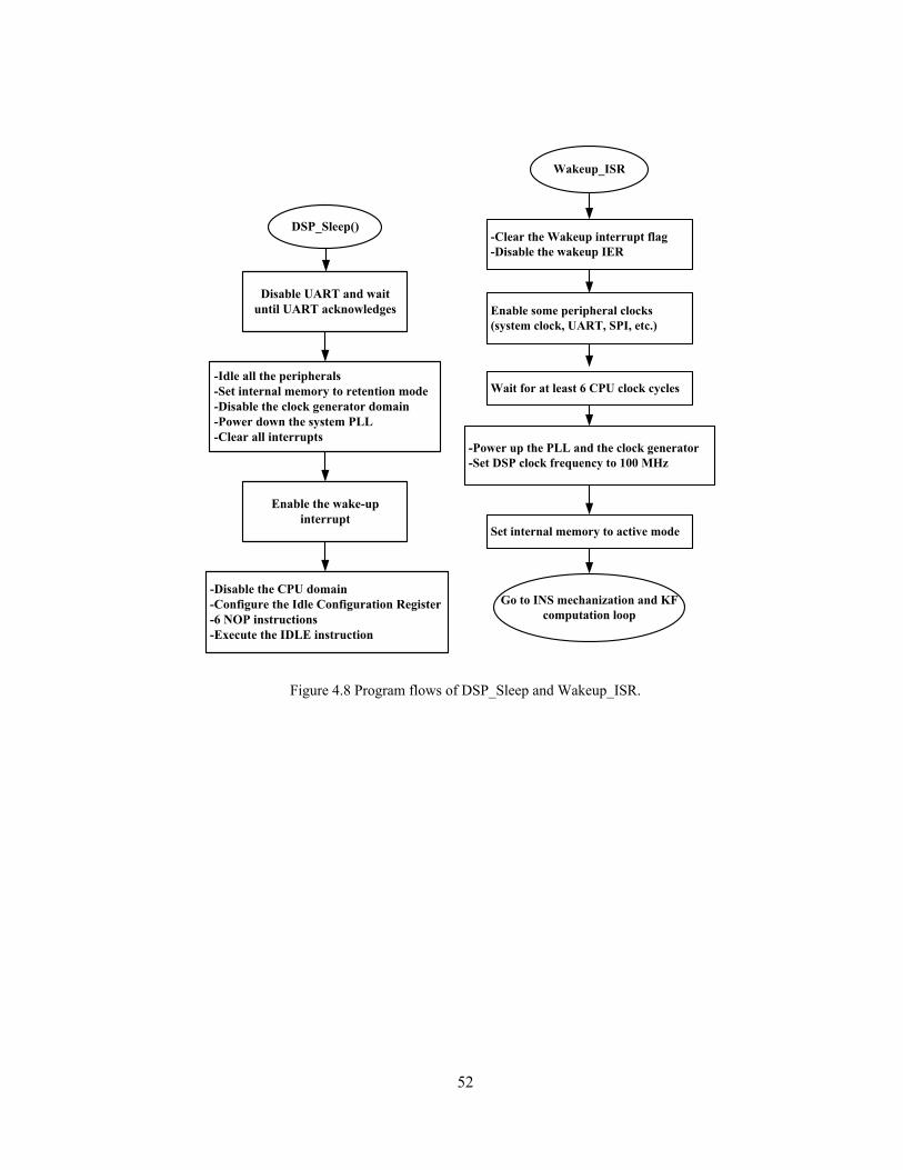
52

Figure 4.8 Program flows of DSP_Sleep and Wakeup_ISR.

53

Figure 4.9 Software flow of the whole system.

4.3.3 DSP Memory Allocation

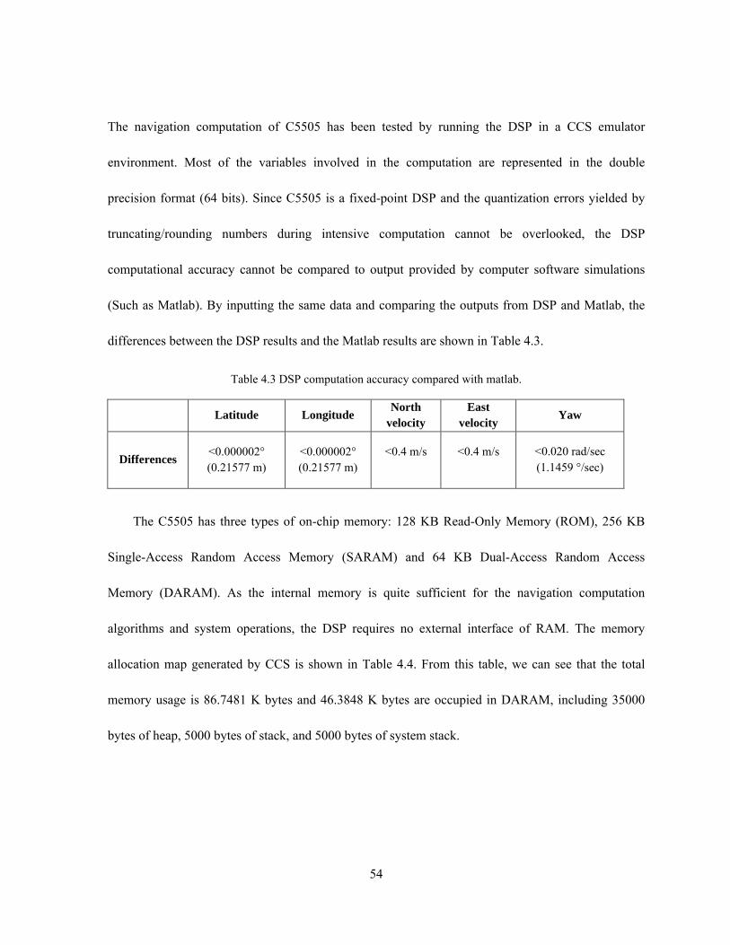
54

The navigation computation of C5505 has been tested by running the DSP in a CCS emulator

environment. Most of the variables involved in the computation are represented in the double

precision format (64 bits). Since C5505 is a fixed-point DSP and the quantization errors yielded by

truncating/rounding numbers during intensive computation cannot be overlooked, the DSP

computational accuracy cannot be compared to output provided by computer software simulations

(Such as Matlab). By inputting the same data and comparing the outputs from DSP and Matlab, the

differences between the DSP results and the Matlab results are shown in Table 4.3.

Table 4.3 DSP computation accuracy compared with matlab.

Latitude Longitude North

velocity East

velocity Yaw

Differences <0.000002° (0.21577 m)

<0.000002° (0.21577 m)

<0.4 m/s

<0.4 m/s

<0.020 rad/sec (1.1459 °/sec)

The C5505 has three types of on-chip memory: 128 KB Read-Only Memory (ROM), 256 KB

Single-Access Random Access Memory (SARAM) and 64 KB Dual-Access Random Access

Memory (DARAM). As the internal memory is quite sufficient for the navigation computation

algorithms and system operations, the DSP requires no external interface of RAM. The memory

allocation map generated by CCS is shown in Table 4.4. From this table, we can see that the total

memory usage is 86.7481 K bytes and 46.3848 K bytes are occupied in DARAM, including 35000

bytes of heap, 5000 bytes of stack, and 5000 bytes of system stack.

55

Table 4.4 Memory map report generated from CCS.

Name Origin (bytes) Length (bytes) Used (bytes, Hex) Used (bytes, Dec) MMR 00000000 000000c0 00000000 0

DARAM 000000c0 0000ff40 0000b98a 46.3848 K SARAM 00030000 0001e000 0000a174 40.3633 K

SAROM_0 00fe0000 00008000 00000000 0 SAROM_1 00fe8000 00008000 00000000 0 SAROM_2 00ff0000 00008000 00000000 0 SAROM_3 00ff8000 00008000 00000000 0 Bytes occupied in total 86.7481 K

4.3.4 Zigbee Node Software Design

A typical Zigbee sensor network is composed of three logical device types, i.e. coordinator, router

and end device. This section presents the software flow of sensor nodes, routers and sink node in

Zigbee networks. The sink node works as the coordinator, while sensor nodes work as the end devices,

which are shown in Figure 4.10.

Sink Node

SmartRF04EB with CC2430EM from TI [43] is used to develop and debug the sink node programs in

this work. It will initialize the board hardware configurations, create a network identifier, and

broadcast PAN ID to start up the network. When the power is turned on, this coordinator will scan all

channels and choose the one with the least energy level. If there are more than one channel with low

energy level, it will choose the channel with the least existing ZigBee networks.

56

Figure 4.10 The structure of a typical ZigBee sensor network

with the coordinator (in black), the routers (in grey) and the end devices (in white).

The task system is based on the multitask mechanism, and its main loop operates in the

Operating System Abstraction Layer (OSAL) which implements a cooperative, round robin task

servicing loop. Each OSAL task has to be initialized first, including initialization of application object

variables, instantiation of the corresponding application object(s), and registration with the applicable

OSAL or Hardware Abstraction Layer (HAL) system services. User defined events will be added into

the task event processor to process all events for the task. The initialization and configuration of the

sink node program flow is shown in Figure 4.11 and the event processing flow of the sink node task

event handler is shown in Figure 4.12.

57

Figure 4.11 The initialization and configuration of the sink node program flow.

Router

This device is used to allow other devices to join the network and route messages from one node to

another. The routers, as well as end devices, scan the channels to find and join the available network

with the identifier specified by the coordinator. CC2430 demonstration boards (CC2430DB) are used

as the routers to compose the ZigBee networks.

58

Figure 4.12 The event processing flow of the sink node task event handler.

Sensor Node

The sensor node works as an end device in the ZigBee network. This device can only receive and

transmit information to the parent node (routers or the coordinator) and it has no routing

capability.Therefore, it is a battery-powered node and can sleep and wake up according to the

network requirements. The navigation board with a CC2430 RF transceiver is used to work as an end

device in this network. The initialization and configuration of the sensor node program flow is the

same as Figure 4.11 and the event processing flow of its task event handler is shown in Figure 4.13.

59

Figure 4.13 The event processing flow of the sensor node task event handler.

60

Chapter 5

Tests and Results

5.1 Equipment and Setup

The MEMS inertial sensors being used in the laboratory calibration and field test II are the three-axis

±3g accelerometer ADXL335 [44] from Analog Devices Inc. and the single-axis ±300º/s yaw rate

gyroscope LISY300AL [45] from STMicroelectronics. These accelerometer and gyroscopes are

operated on a voltage supply 3.3 V and give 1.5V and 1.65V respectively as their zero-g and zero-rate

voltage level. The sensitivity of the accelerometer and gyroscope is typically 300 mV/g and 3.3

mV/º/s, respectively. The specifications for these analog inertial sensors are shown in Table 5.1. The

analog signals from accelerometers and gyroscopes are sampled by a multi-channel ADC which

processes the inertial sensor measurements and converts them into digital signals. A 14-bit, 285 KSPS

ADC from Analog Devices Inc. (AD7856) [46] is chosen for sampling the inertial sensor

measurements. A multiplexer is used for multi-channel sampling at the input stage of ADC.

Therefore, a time delay ( t) exists between the sampling of two sequential channels [15]. Since the

conversion time ( t) is sufficiently short depending on the master clock signal (max. 6 MHz) for

ADC, the effect of errors due to phase delays is negligible. The specifications for the inertial sensors

and ADC are given in Table 5.1. The GPS receiver used in the tests is LEA-5H from -blox, which

was introduced in Chapter 4.

61

5.2 Real-Time Performance Analysis

The DSP real-time performance was evaluated by CCS C55xx Rev 3.0 Cycle Accurate Simulator.

Each assembly instruction is executed with a certain number of instruction cycles, and the duration of

each mechanization computation and Kalman filtering computation can be calculated by counting the

number of cycles the program takes.

Table 5.1 Specifications for ADXL335 and LISY300AL.

Parameter Typical Value Gyroscope LISY300AL

Measurement range ° Sensitivity °

Zero-rate level 1.65 V Non linearity of full scale Noise density °

Accelerometer ADXL335 Measurement range

Sensitivity 300 mV/g Zero-rate level 1.5 V Non linearity of full scale

Noise density at Xout, Yout μ Noise density at Zout μ

As shown in Table 5.2, the number of instruction cycles required for one mechanization

computation is 84709; one Kalman filtering computation requires 4023352 cycles. When the DSP

runs at 100 MHz, the duration of each instruction cycle is 10 ns. Therefore, the execution time for

each step of mechanization computation takes 0.8 ms while each step of Kalman filtering

computation takes 40 ms. Based on these results, the duration of GPS and INS data reading can be

calculated by running the prototype navigation board, which is introduced in Section 5.1, recording

the time and using the CCS emulator to count how many times the navigation calculation loop repeats

62

in this period. The duration of INS data reading for each time was approximately 4.65 ms on average,

and the program took nearly 90.909 ms to read and parse the GPS data whenever it was updated

(when GPS is available, it will update every second). According to the software design introduced in

Chapter 4, the navigation calculation is running in an infinite loop. In each step, INS reading,

mechanization and Kalman filtering computation will be executed successively. In contrast, GPS data

reading runs in an interrupt service routine. Therefore, when a GPS update is available, DSP with 100

MHz clock rate can run the navigation calculation loop 20 times and get 20 position results (as well

as the velocity and heading information) per second; otherwise, if there is no GPS update, DSP can

get 22 position results per second. Figure 5.1 illustrates the DSP computation time frame.

Table 5.2 Execution time for the Program.

Number of CPU Cycles Execution Time on DSP operated with 100 MHz

Initialization <2 ms

GPS Data Reading 90.909 ms (per second)

INS Data Reading 4.65 ms

Mechanization 84709 0.8 ms

Kalman Filter 4023352 40 ms

Figure 5.1 A typical time frame within one second of DSP computation.

5.3 Navigation Board Calibration

5.3.1 Test Setup

63

The inertial sensors and ADC used in this test were the three-axis accelerometer ADXL335, the

single-axis gyroscope LISY300AL and the 14-bit ADC AD7856, which are introduced in Section 5.1.

The local gravity used for computing the deterministic error parameters was calculated by the given

altitude and latitude provided by the GPS, as follows [47]:

(5.1)

where,

lat and alt denote the latitude in degrees and the altitude in meters respectively,

g denotes the earth’s gravity in at the location that is specified by certain latitude and

altitude, and

a1, a2, a3, a4, a5 and a6 are normal gravity constants, which is given in Table 5.3.

Table 5.3 Normal gravity constants.

Constant a1 a2 a3

Value 9.7803267714 0.0052790414 0.0000232718

Constant a4 a5 a6

Value -0.000003087691089 0.000000004397731 0.000000000000721

5.3.2 Multi-Position Static Test Results

The static test was carried out in the laboratory and the duration of this test at each position was 15

minutes. The average values of these static data from the 3-axis accelerometer were used to calculate

64

the deterministic error coefficient matrix M with the least-square method, according to Equation

(3.11). The result is shown below:

(5.2)

Based on Equation (5.2), a summary of the deterministic error parameters obtained from the six

position static test is shown in Table 5.4.

5.3.3 Random Error Modeling

As introduced in Section 3.3, in order to derive the first order GM model parameters, i.e. noise

variances and correlation times of MEMS gyroscope and accelerometer, an experimental dataset

Table 5.4 Parameters used in accelerometer’s deterministic errors.

Acc.X Acc.Y Acc.Z

Biases (m/s2) -0.3942 0.4322 -0.0122 Scale Factor Error (%) -1.85 0.38 -0.29

Non-Orthogonalities (%)

m.xy m.xz m.yx m.yz m.zx m.zy -0.08 -1.91 0.20 0.43 3.30 0.59

was collected from a 2-hour static test to estimate the ACS of inertial sensor errors. By removing the

bias offsets from the raw measurements, the ACSs of 2-axis accelerometer and gyroscope can be

calculated by Equation (5.3) and they are shown Figure 5.2, 5.5 and 5.7 respectively. From these

three plots, the noise variance of 1st order GM process can be determined directly at t=0 and

correlation time can be obtained when R(τ) = σ . By enlarging Figure 5.2 and 5.5, this procedure

is clearly shown in Figure 5.4 and 5.6. As shown in Table 5.5, these parameters were then used to

model the stochastic errors of inertial sensors in the field test II.

65

Table 5.5 First order GM model parameters used in field test II.

Acc.X Acc.Y Gyro.Z

Noise Variance 0.002062596 0.001597938 0.163237989

Correlation Time (sec.) 981.7 478 <100

(5.3)

where,

is a discrete signal with N sample measurements,

is the ACS of the discrete signal ,

E[] is the mathematical expectation operator, and

m is the time lag (shift) between samples.

Figure 5.2 The autocorrelation of x-axis accelerometer reading of 2-hour stationary dataset

after removing the bias offset.

-8000 -6000 -4000 -2000 0 2000 4000 6000 8000-0.5

0

0.5

1

1.5

2

2.5x 10

-3

t in seconds

Aut

ocor

rela

tion

R(t

)

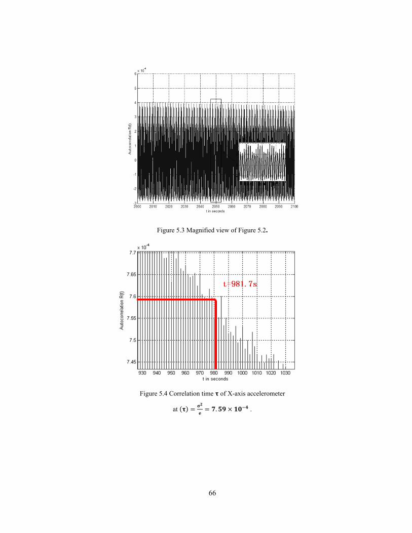
66

Figure 5.3 Magnified view of Figure 5.2.

Figure 5.4 Correlation time of X-axis accelerometer

at .

67

Figure 5.5 The autocorrelation of y-axis accelerometer reading of 2-hour stationary dataset


Figure 5.6 Correlation time of Y-axis accelerometer

at .

-8000 -6000 -4000 -2000 0 2000 4000 6000 8000-4

-2

0

2

4

6

8

10

12

14

16x 10

-4

t in seconds

Aut

ocor

rela

tion

R(t

)

68

Figure 5.7 The autocorrelation of z-axis gyroscope reading of 2-hour stationary dataset


5.4 Open Field Tests

Data from open area tests are being studied and analyzed. Besides, trajectories generated by the

navigation board in the real-time scenario are also depicted in this section. Dataset I was provided by

Walid Farid Abd El Fatah from Dr. Aboelmagd Noureldin’s laboratory at Royal Military College

(RMC), Kingston, Canada. This test is to assess the positioning accuracy of the 2D mechanization

and the Kalman filter algorithm with accurate acceleration and angular rate inputs. Moreover, field

tests using the prototype system, which is introduced in Section 5.1, were conducted and repeated for

many times. Dataset II is a good example of those test results. The third test is to evaluate the

performance of the proposed navigation board that is introduced in Chapter 4. The navigation

performance to bridge GPS outage has been verified by all those experiments.

-8000 -6000 -4000 -2000 0 2000 4000 6000 8000-0.02

0

0.02

0.04

0.06

0.08

0.1

0.12

0.14

0.16

0.18

t in seconds

Aut

ocor

rela

tion

R(t

)

69

5.4.1 Field Test I

5.4.1.1 Test Setup and Description

To examine the effectiveness of the navigation frame INS mechanization and the aforementioned

Kalman filter for 2D INS/GPS integration solution, field test I was carried out with MEMS-grade

IMU and wheel encoders to provide the angular rate and acceleration of the vehicle. The vehicle used

in this test is a three-wheel robot and its movement is controlled by a joystick and the motors are

powered by four rechargeable storage batteries. This vehicle was equipped with the Xbow

IMU300CC-100 and wheel encoders to provide the INS raw measurements. The Xbow IMU was

used to measure the heading angle and the forward acceleration was calculated with respect to the

velocity measurements from the wheel encoders. The specification for IMU300CC-100 is given in

Table 5.6.

Table 5.6 Specifications for XBow IMU300CC-100.

Xbow IMU300CC-100

Specification Value

Update Rate (Hz) > 100 Range ( ) 100

Bias ( ) < 2.0

Scale Factor Accuracy (%) < 1

Non-Linearity (% FS) < 0.3

Resolution ( ) < 0.025

Bandwidth (Hz) >25

Random Walk ( ) <2.25 Typical

70

Table 5.7 GPS/IMU specifications of the reference system.

IMU HG1700 Specifications Gyroscope Accelerometer Range 1,000 deg/sec 50g Bias 1.0 deg/hr 1.0 mg Scale Factor 150 ppm 300 ppm Angle/Velocity Random Walk

0.125 deg/ No spec

Linearity No spec 500 ppm GPS NovAtel OEM4

Technical Specifications 24-Channel L1/L2 C/A Code with full Carrier Tracking Pulse Aperture CorrelatorTM Data Rate 20 Hz Position Accuracy DGPS (L1, C/A) 0.45 m CEP Velocity Accuracy 0.03 m/s RMS

The duration of this test is 9 minutes and 41 seconds and the overall distance was approximately

400 meters. The reference system used in this test to access the navigation solution is composed of

the Novatel OEM4 GPS receiver and the Honeywell HG1700 tactical grade IMU. The specification

of the reference system is given by Table 5.7.

5.4.1.2 Results and Analysis

By comparing the measurements and outputs from the reference system introduced in the previous

section with the outputs provided by the integrated filter, this section will discuss the performance of

the navigation algorithm in terms of longitude, latitude, velocities and the heading angle. The

emphasis of this section is placed on the estimation accuracies of the navigation system during the

absence of GPS updates.

As mentioned in Chapter 1, to maintain reliable performance of the KF prediction, the GPS

aiding information should be available at all times. However, the sky is often masked by various

71

obstructions such as trees and buildings. This will result in the partial or complete loss of satellite

visibility. In these cases, it is important to know the impact on the navigation results when a GPS

update is absent and the filter works in a full prediction mode. Therefore, several simulated GPS

outages were artificially conducted into the trajectory to assess the prediction accuracy of the

navigation system.

Figure 5.8 demonstrates and compares the trajectories provided by the integrated filter and the

reference system. As shown in this figure, the movement of the vehicle was simple: it only moved

along straight lines and turned with 90-degree angles in the test. There are four GPS outages with 60-

second durations in the trajectory. Two of them happened during the straight-line motion and the

other two outages covered the first and the third cornering motions.

Figure 5.9 and 5.12 give a further representation of the position errors and velocity errors

respectively, based on the reference results. Figure 5.9 shows that when the GPS signals were not

available, the position errors accumulated with the course of time until the system regained the GPS

updates. The only exception is the second GPS signal gap. The errors reached the maximum value

when the vehicle was turning the corner. The errors started to reduce when the vehicle ran back into a

straight line.

In addition, the horizontal velocities and the yaw angles from the EKF results and the reference

outputs are depicted in Figure 5.10, 5.11 and 5.13. It may be noticed that when GPS updates are

available, both the north velocity and the east velocity obtained from the EKF and the reference

system closely overlap, which results in very few position errors, as shown in Figure 5.8 and 5.9.

72

Figure 5.13 clearly shows that the yaw angle calculated by the integrated filter was almost the same

as the reference outputs, even during the GPS outages.

Figure 5.8 Field test I: Reference trajectory and KF trajectory with 4 simulated GPS outages.

Figure 5.9 Field test I: North/East position errors.

0 100 200 300 400 500 6000

5

10

15

20

25

30

Time in Seconds

Nor

th/E

ast

Err

ors

in M

etre

s

GPS Outage Zone

North Errors

East Errors

73

Figure 5.10 Field test I: Reference north velocity and KF north velocity.

Figure 5.11 Field test I: Reference east velocity and KF east velocity.

74

Figure 5.12 Field test I: East/North velocity errors.

Figure 5.13 Field test I: Reference yaw and KF yaw.

0 100 200 300 400 500 6000

0.2

0.4

0.6

0.8

1

1.2

1.4

1.6

1.8

2

Time in Seconds

Err

ors

of V

e/V

n in

Met

res/

Sec

GPS Outage Zone

Errors of Ve

Errors of Vn

75

Table 5.8 shows the mean, RMS and maximum values of the position and velocity errors

provided by EKF during four GPS outages. Generally, it can be determined from this table that the

positioning results during 60-second GPS outage periods are accurate. The RMS values are less than

9 meters and the maximum errors are less than 14 meters.

Table 5.8 Field test I: Position/Velocity errors during GPS outages.

Outage 1 Outage 2 Outage 3 Outage 4

North Position

Errors

in Meters

Mean 0.270

RMS 0.320

Max. 0.709

Mean 2.969

RMS 3.675

Max. 7.282

Mean 1.131

RMS 1.461

Max. 2.430

Mean 0.622

RMS 0.776

Max. 1.862

East Position

Errors

in Meters

Mean 2.267

RMS 2.868

Max. 5.638

Mean 6.881

RMS 8.133

Max. 13.450

Mean 3.862

RMS 4.751

Max. 8.362

Mean 2.418

RMS 3.047

Max. 6.801

Position Errors

in Meters

Mean 2.329

RMS 2.886

Max. 5.646

Mean 7.918

RMS 8.924

Max. 13.881

Mean 4.034

RMS 4.971

Max. 8.637

Mean 2.545

RMS 3.144

Max. 6.959

North Velocity

Errors in M/Sec

Mean 0.038

RMS 0.044

Max. 0.093

Mean 0.238

RMS 0.342

Max. 0.927

Mean 0.222

RMS 0.262

Max. 0.402

Mean 0.069

RMS 0.092

Max. 0.350

East Velocity

Errors in M/Sec

Mean 0.104

RMS 0.110

Max. 0.225

Mean 0.436

RMS 0.476

Max. 0.733

Mean 0.275

RMS 0.306

Max. 0.568

Mean 0.212

RMS 0.242

Max. 0.483

5.4.2 Field Test II

5.4.2.1 Test Description

The navigation system used in this test is composed of ADXL335, LISY300AL, AD7856 and GPS

LEA-5H. Details are mentioned previously in Section 5.1. The DSP used in this test is

76

TMS320VC5505EVM, which is the evaluation module of C5505 from TI. Inertial sensors were

mounted on a 4-wheel cart. The GPS antenna was mounted on the top layer of this cart. Data

acquisition was carried out using DSP to read both INS and GPS data. A laptop provided the power

for the whole prototype board and recording the data sent from DSP C5505.

This field test was carried out along the racetrack around the soccer field, on the main campus of

Queen’s University in Kingston, ON, which is an open area with a sufficient number of satellites

available throughout the entire time period of the test. The average speed for this test was 1.45 meters

per second. Vibration of the inertial sensors was minimal due to the flatness of the ground. The test

duration was 4 minutes and 41 seconds and the total distance travelled was approximately 400 meters.

5.4.2.2 Results and Analysis

Both trajectories obtained from the KF with and without the use of NHC are depicted in Figure 5.14.

Similarly to the first test, four 20-second GPS outage scenarios were simulated at different locations

along the trajectory to evaluate the performance of the navigation solution when GPS signals are

absent. In addition, the position/velocity errors of the test results with and without the use of NHC are

given and compared in Figure 5.15, 5.16, 5.19 and 5.20. It is clearly shown that the errors increased

rapidly and with high amplitude during GPS outages.

Figure 5.17, 5.18, 5.21 compare north velocity, east velocity and the yaw angle obtained from

the three scenarios (GPS, KF, KF with the use of NHC) respectively. In Figure 5.17 and 5.18, it is

clearly shown that the velocities provided by the integration filter deviate from the GPS outputs

during the signal outages.

77

Figure 5.14 Field test II: GPS trajectory and KF trajectories with 4 simulated GPS outages.

Figure 5.15 Field test II: North position errors.

0 50 100 150 200 250 3000

5

10

15

20

25

30

Time in Seconds

Nor

th E

rror

s in

Met

res

GPS Outage Zone

North

North(NHC)

78

Figure 5.16 Field test II: East position errors.

Figure 5.17 Field test II: GPS north velocity and KF north velocity.

0 50 100 150 200 250 3000

5

10

15

20

25

30

Time in Seconds

Eas

t E

rror

s in

Met

res

GPS Outage Zone

East

East(NHC)

79

Figure 5.18 Field test II: GPS east velocity and KF east velocity.

Figure 5.19 Field test II: north velocity errors.

0 50 100 150 200 250 3000

0.2

0.4

0.6

0.8

1

1.2

1.4

1.6

1.8

2

Time in Seconds

Err

ors

of V

n in

Met

res/

Sec

GPS Outage Zone

Errors of Vn

Errors of Vn(NHC)

80

Figure 5.20 Field test II: east velocity errors.

Figure 5.21 Field test II: GPS yaw and KF yaw.

0 50 100 150 200 250 3000

0.2

0.4

0.6

0.8

1

1.2

1.4

1.6

1.8

2

Time in Seconds

Err

ors

of V

e in

Met

res/

Sec

GPS Outage Zone

Errors of Ve

Errors of Ve(NHC)

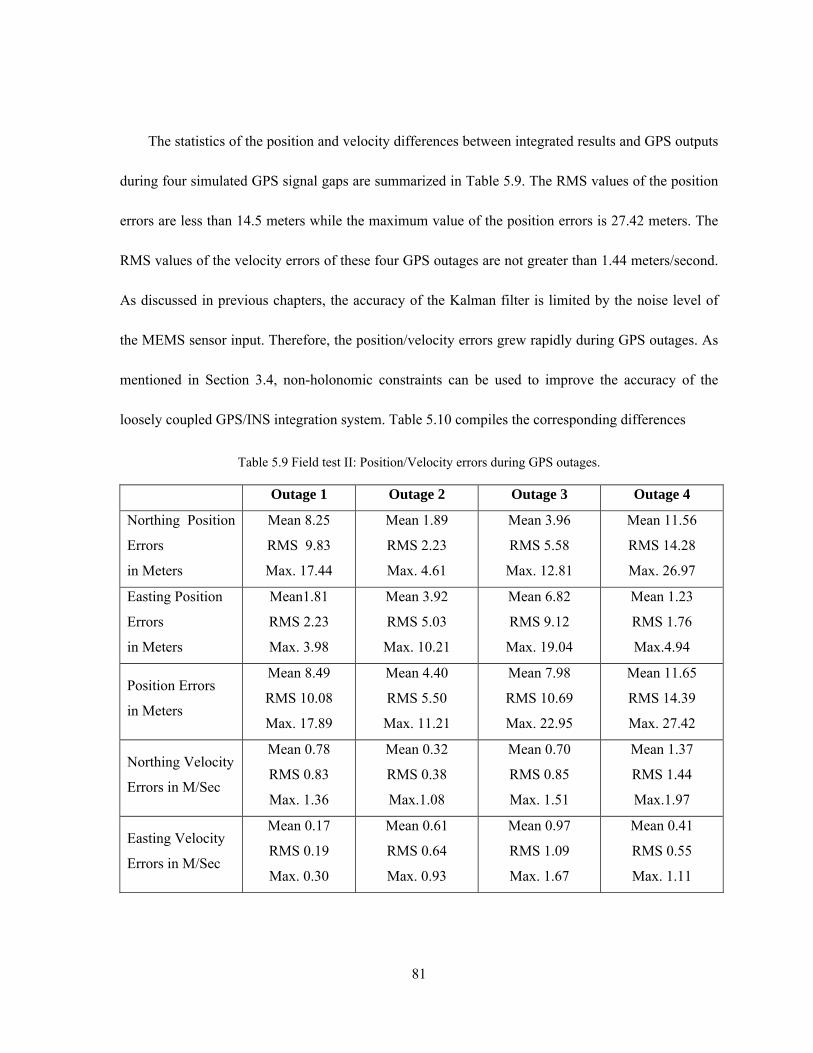
81

The statistics of the position and velocity differences between integrated results and GPS outputs

during four simulated GPS signal gaps are summarized in Table 5.9. The RMS values of the position

errors are less than 14.5 meters while the maximum value of the position errors is 27.42 meters. The

RMS values of the velocity errors of these four GPS outages are not greater than 1.44 meters/second.

As discussed in previous chapters, the accuracy of the Kalman filter is limited by the noise level of

the MEMS sensor input. Therefore, the position/velocity errors grew rapidly during GPS outages. As

mentioned in Section 3.4, non-holonomic constraints can be used to improve the accuracy of the

loosely coupled GPS/INS integration system. Table 5.10 compiles the corresponding differences

Table 5.9 Field test II: Position/Velocity errors during GPS outages.


Northing Position

Errors

in Meters

Mean 8.25

RMS 9.83

Max. 17.44

Mean 1.89

RMS 2.23

Max. 4.61

Mean 3.96

RMS 5.58

Max. 12.81

Mean 11.56

RMS 14.28

Max. 26.97

Easting Position

Errors

in Meters

Mean1.81

RMS 2.23

Max. 3.98

Mean 3.92

RMS 5.03

Max. 10.21

Mean 6.82

RMS 9.12

Max. 19.04

Mean 1.23

RMS 1.76

Max.4.94

Position Errors

in Meters

Mean 8.49

RMS 10.08

Max. 17.89

Mean 4.40

RMS 5.50

Max. 11.21

Mean 7.98

RMS 10.69

Max. 22.95

Mean 11.65

RMS 14.39

Max. 27.42

Northing Velocity

Errors in M/Sec

Mean 0.78

RMS 0.83

Max. 1.36

Mean 0.32

RMS 0.38

Max.1.08

Mean 0.70

RMS 0.85

Max. 1.51

Mean 1.37

RMS 1.44

Max.1.97

Easting Velocity

Errors in M/Sec

Mean 0.17

RMS 0.19

Max. 0.30

Mean 0.61

RMS 0.64

Max. 0.93

Mean 0.97

RMS 1.09

Max. 1.67

Mean 0.41

RMS 0.55

Max. 1.11

82

Table 5.10 The accuracy improvement with NHC.


Latitude Error

in Meters

Mean 0.05311

RMS 0.07152

Max. 0.16383

Mean -0.15141

RMS 0.25123

Max. 0.37841

Mean -2.73988

RMS -4.27284

Max. -10.46811

Mean -2.71550

RMS -3.29470

Max. -6.41486

Longitude Error

in Meters

Mean 0.06345

RMS 0.08462

Max. 0.18479

Mean -1.43684

RMS -1.84654

Max. -3.63789

Mean 0.35443

RMS 0.51679

Max. 1.29497

Mean -0.02630

RMS -0.08213

Max. -0.16886

Position Error

in Meters

Mean 0.06614

RMS 0.08871

Max. 0.20141

Mean -1.31906

RMS -1.46655

Max. -2.95220

Mean -0.44483

RMS -0.96712

Max. -2.47791

Mean -2.68400

RMS -3.27541

Max. -6.31721

North Velocity

Error in M/Sec

Mean 0.00881

RMS 0.00960

Max. 0.01426

Mean 0.02552

RMS 0.06688

Max. 0.09853

Mean -0.48160

RMS -0.55773

Max. -0.92419

Mean -0.30842

RMS -0.33708

Max. -0.52490

East Velocity

Error in M/Sec

Mean 0.00820

RMS 0.00923

Max. 0.01536

Mean -0.18625

RMS -0.20072

Max. -0.28659

Mean 0.06667

RMS 0.08750

Max. 0.20073

Mean -0.00213

RMS 0.01225

Max. 0.04880

between the position/velocity error statistics provided by the Kalman filter with and without the use

of NHC to assess the accuracy improvement. Based on the data set shown in this table, we can see

that both velocity and position estimations of the KF with NHC give better results in comparison with

the KF algorithm that does not use NHC, although in some cases they provide a comparable level of

accuracy. It can be concluded that non-holonomic constraints guarantee an improved performance

during short term GPS outages.

5.4.3 Field Test III

5.4.3.1 Test Description

83

Several field tests were carried out to evaluate the performance of the navigation board which is

introduced in Chapter 4. The first 3 tests shown in this section were conducted by a person on foot, at

the same place as field test II (the racetrack around the soccer field, on the main campus of Queen’s

University). The other 3 road trajectory tests were carried out in a land-vehicle, near the main

campus of Queen’s University, Kingston.

In these tests, GPS LEA-5H was integrated with the navigation board and inertial sensors

ADIS16003, ADIS16060 and HMC6352 were used to provide the acceleration, the angular rate, and

the heading angle respectively. Another GPS -blox EVK-5H was used as a reference to compare the

positioning performance with the navigation board. A laptop provided the power for the GPS EVK-

5H and CC2430EM-SmartRF04EB which is used to receive the position data sent from the

navigation board. The equipment setup is shown in Figure 5.22.

Figure 5.22 Equipment setup for the field test.

5.4.3.2 Test Results

84

Three datasets of those trajectories obtained from the GPS EVK-5H and the navigation board with the

on-foot scenario are depicted in Figure 5.23, Figure 5.24 and Figure 5.25. Several GPS outages took

place at different locations along the trajectory and the average outage duration was around 30

seconds. Figure 5.26, Figure 5.27 and Figure 5.28 show the trajectories for the in-vehicle scenario.

Table 5.12 and Table 5.13 summarize the position differences between the navigation board outputs

and GPS reference outputs during all the GPS outages. The average position errors of the outages in

each trajectory are also included. Although the position errors exceed 20 meters during 30-second

GPS outages due to the use of the low-cost MEMS-based inertial sensors, the results still illustrate the

reliability of this proposed hardware system in providing accurate navigation solution.

Table 5.11 Specifications for ADIS16003, ADIS16060 and HMC6352.

Parameter Typical Value Gyroscope ADIS16060

Measurement range ° Sensitivity °

Drift ° Angular Rate Random Walk °

Accelerometer ADIS16003 Measurement range

Sensitivity 820 LSB/g Zero g Bias Stability

Acceleration Random Walk at Xout, Yout μ Magnetic Sensor HMC6352

Heading Accuracy 2.5 degRMS Heading Resolution 0.5 deg

Disturing Field min 20 gauss Max. Exposed Field max 10,000 gauss

85

Figure 5.23 Test III.1: GPS trajectory and on-foot Trajectory with 6 GPS outages.

Figure 5.24 Test III.2: GPS trajectory and on-foot trajectory with 5 GPS outages.

-76.4992 -76.499 -76.4988 -76.4986 -76.4984 -76.4982 -76.498 -76.4978 -76.497644.2255

44.226

44.2265

44.227

44.2275

44.228

Longitude in Degrees

Latit

ude

in D

egre

es

NavPCB

GPS REFGPS Outages

-76.4994-76.4992 -76.499 -76.4988-76.4986-76.4984-76.4982 -76.498 -76.4978-76.4976-76.497444.2256

44.2258

44.226

44.2262

44.2264

44.2266

44.2268

44.227

44.2272

44.2274

44.2276


Latit

ude

in D

egre

es

NavPCB

GPS REFGPS Outages

86

Figure 5.25 Test III.3: GPS trajectory and on-foot trajectory with 5 GPS outages.

Figure 5.26 Test III.4: GPS trajectory and in-vehicle trajectory with 5 GPS outages.

-76.4992 -76.499 -76.4988 -76.4986 -76.4984 -76.4982 -76.498 -76.4978 -76.497644.2258

44.226

44.2262

44.2264

44.2266

44.2268

44.227

44.2272

44.2274

44.2276


Latit

ude

in D

egre

es

NavPCB

GPS REFGPS Outages

87



88

Table 5.12 On-foot field test: Position errors during GPS outages.

Trajectory 1

Outage 1 Outage 2 Outage 3 Outage 4 Outage 5 Outage 6

Outage Duration in Seconds 28 33 34 26 28 29

Position Error in Meters 8.588 26.870 18.892 29.812 13.181 17.531

Average Position Error in Meters 19.146

Trajectory 2

Outage 1 Outage 2 Outage 3 Outage 4 Outage 5 Outage Duration

in Seconds 32 34 27 31 33

Position Error in Meters 16.419 13.794 10.570 23.349 20.605

Average Position Error

in Meters 16.947

Trajectory 3


in Seconds 34 31 31 35 31


Average Position Error

in Meters 25.845

89

Table 5.13 In-vehicle field test: Position errors during GPS outages.

Trajectory 4

Outage 1 Outage 2 Outage 3 Outage 4 Outage 5

Outage Duration in Seconds 24 28 34 36 30



Trajectory 5

Outage 1 Outage 2 Outage 3 Outage 4 Outage Duration

in Seconds 32 29 35 34

Position Error in Meters 30.900 25.692 33.308 26.803


Trajectory 6


in Seconds 29 32 32 29 33



5.5 Summary

The objective of the field tests was to evaluate the navigation performance of the integrated system

using low-cost MEMS inertial sensors and the GPS. Open area tests are discussed in this chapter to

investigate the system performance with different GPS signal visibilities. Many experiments were

repeated and the overall system performance results were positive. In this chapter, the results of three

field tests were presented. These results were compared based on INS-only navigation and therefore,

several simulated GPS outage periods were intentionally inserted into the first and second tests. In the

third test, the GPS outages were inserted by removing GPS directly from the navigation board. For

90

the first test, wheel encoders and a high-performance MEMS gyroscope were used and the outage

duration was 60 seconds. The maximum RMS value of the position errors among all these 4 outages

is 8.9 meters. If the vehicle ran in a straight line, the maximum RMS value of the position errors was

less than 5 meters. The second test used more compact and less expensive MEMS inertial sensors to

provide the accelerations and the angular rate. A successful 2D KF algorithm was presented, as well

as the constraints of the vehicle motion being employed in the second field test, which decreased the

position/velocity errors to some extent. Due to the error propagation characteristics of MEMS sensors,

the errors quickly grew when 20-second GPS signal gaps were inserted. However, control of the

navigation errors was sufficient during short GPS outages. The maximum RMS value of the position

errors was less than 11.5 meters. The results also show that the navigation errors are reduced by NHC

during GPS outages, with an average improvement level of approximately 1.4 meters. The third test

evaluated the real-time performance of the navigation board. The results from the trajectories show

that by using the navigation board, the average position errors during roughly 30-second GPS outages

are approximately 20.6 meters for the on-foot scenario and 26.7 meters for the in-vehicle scenario.

91

Chapter 6

Summary, Conclusions and Recommendations

6.1 Summary of Conclusions

The main contribution of this thesis is to propose an integrated system architecture for GPS/INS-

enable WSN. This hardware architecture is a recommended implementation method for location-

based WSN since it is highly optimized for dimension, real-time computation and energy efficiency.

Besides, the INS/GPS integration makes the system capable to get reliable navigation information

when GPS signals are weak or blocked. The proposed system uses a single DSP chip for both the data

acquisition and inertial navigation computations. A fifteen state Kalman filter was designed using the

perturbation theory model for position, velocity and attitude. Field tests were also carried out to

assess the real-time performance and the overall system accuracy. GPS outages were simulated and

the INS prediction accuracy was evaluated for the field data.

The issues regarding GPS/INS integration, software/hardware implementation, real-time

performance and field test results are summarized below:

1. The proposed system is optimized for dimension, real-time computation and power consumption,

which are the focal concerns in energy-constrained sensor networks. A loosely coupled GPS/INS

integrated approach is applied to estimate the position, velocity and attitude. This navigation

board uses a fixed-point DSP with a clock rate of 100 MHz to perform the navigation calculation

and one single power supply of 4.5V is used to feed all the circuit boards. MEMS sensors are

used in this proposed system to reduce the overall cost, weight and power consumption.

92

2. When the system is employed in an urban canyon or forest, where GPS becomes unavailable due

to signal blockages, the integration accuracy is degraded. In the first scenario in Chapter 5, the

vehicle used wheel encoders and a high-performance MEMS gyroscope to obtain the

acceleration and angular rate. Based on the trial results, the average position error of this

proposed system was 5 meters during a 60-second GPS outage. The largest RMS value of the

position error among the four outages was less than 9 meters. In the second test, when less

expensive inertial sensors were used and the average speed of the vehicle was approximately

1.45 meters/second, the position error was 10.17 meters on average during a 20-second GPS

outage. The largest RMS value of position errors among the four outages was less than 14.5

meters.

3. Low-power design: a PIC microcontroller is used to detect the external-interrupt triggered

motion/acceleration of the navigation board and control the power supplies of various circuits

and ICs. The motion detection scheme takes advantage of the ultra-low-power wake-up feature

of MCU PIC16F886, which significantly decreases the power consumption of the board when it

remains stationary.

4. Real-time performance: The DSP works on a 100 MHz clock rate and the Kalman filter was

executed every 47.6 ms. This is well within the real-time requirements and achieves positioning

accuracy. The GPS updates once per second whenever it is available.

5. An RF transceiver is integrated into the navigation board. Therefore, this system can be used in

Zigbee sensor networks. Each moving end device can send its positioning data to the cluster

header/network coordinator over the air.

93

6. The stand-alone INS position errors can be decreased by the use of non-holonomic constraints.

Based on the test results in Chapter 5, the non-holonomic constraints provided a better

navigation solution and it achieved an average improvement of approximately 1.4 meters during

the GPS outages.

7. The real-time tests by using the proposed navigation board with the improvement provided by a

magnetic sensor have been carry out to evaluate the system performance with actual sensor

inputs. The results show that the average position error during a 30-second GPS outage is

approximately 20.6 meters for the on-foot scenario and 26.7 meters for the in-vehicle scenario.

6.2 Developed Programs

The following is a list of programs developed for implementing and testing the embedded system:

1. A motion detection program based on MPLAB IDE that can detect the motion of the board and

manage the system power (Chapter 4)

2. A navigation system program developed in CCS that includes DSP initialization and

configurations, ISRs, data acquisition, data parsing, navigation computation algorithms,

communications and interfaces with the PIC MCU and CC2430 (Chapter 4)

3. Programs developed in IAR Embedded Workbench that describe the application layer of end

devices, routers and the coordinator based on ZigBee sensor networks, as well as interface

programs for the CC2430 MCU to communicate with the external flash memory and DSP

(Chapter 4)

94

4. A Matlab-based loosely coupled EKF that is used to simulate and analyze the system

performance of the GPS/INS integrated solution (Chapter 5)

5. A program that logs and analyzes the static data from inertial sensors to estimate the

deterministic error parameters and the random error parameters for 1st order GM model (Chapter

5)

6.3 Recommendations for Future Work

Based on the results presented in the previous chapters, the following recommendations for future

work to improve the performance of the proposed navigation system are made and listed as follows:

1. As discussed in Chapter 3, initial calibration and stochastic error modeling are essential to

improve the KF prediction accuracy during GPS outages. Although the 1st order GM model

reduces the computational complexity of the Kalman filter, using higher order GM models or AR

models will provide better results, which can be compared with the traditional 1st order GM

model regarding the accuracy improvement.

2. Low cost MEMS inertial sensors have run-to-run biases. An efficient way to calibrate the sensor

biases is to use on-line GPS data to calibrate the bias errors and reset them in real-time.

3. A 3D solution for the GPS/INS integration scheme with 6 degree-of-freedom inertial sensor

array can be applied to the system and the navigation results will be compared with a 2D solution

to determine whether and to what degree it can improve the integration accuracy during GPS

outages.

95

4. A possible extension of this work would be to investigate new methods to improve the accuracy

of this navigation solution during GPS outages, without significantly increasing the computation

complexity of the algorithm.

96

Bibliography

1. Ko, Y.B. and N.H. Vaidya, Location-Aided Routing (LAR) in mobile ad hoc networks. Wireless Networks, 2000. 6(4): p. 307-321.

2. Zorzi, M. and R.R. Rao, Geographic random forwarding (GeRaF) for ad hoc and sensor networks: Multihop performance. Ieee Transactions on Mobile Computing, 2003. 2(4): p. 337-348.

3. V.Hnatyshin, H.A., Design and Implementation of an OPNET model for simulating GeoAODV MANET routing Protocol, in Proc. of the OPNETWORK 2010 International Conference, Session: Wireless Ad Hoc and Wireless Personal Area Networks. August, 2010: Washington DC.

4. Dipankar Deb, S.B.R., NabenduChaki, LACBER: A New Location Aided Routing Protocol for GPS Scarce MANET. International Journal of Wireless & Mobile Networks (IJWMN), August 2009. 1.

5. Zhang, G., A Low Cost Integrated INS/GPS System. UCGE Reports Number 20078, 1995. 6. Elkaim, G.H., M. Lizarraga, and L. Pederseny, Comparison of low-cost GPS/INS sensors for

Autonomous Vehicle applications. Position, Location and Navigation Symposium, 2008 IEEE/ION 2008: p. 1133-1144.

7. Kelley, R.T., I.N. Katz, and C.A. Bedoya, Design, development and evaluation of an Ada coded INS/GPS open loop Kalman filter, in Proceedings of the IEEE 1990 National, Aerospace and Electronics Conference. 1990. p. 382-388.

8. Chatfield, A., Fundamentals of High Accuracy Inertial Navigation. 1997: American Institute of Aeronautics and Astronautics.

9. Rogers, R.M., Applied mathematics in integrated navigation systems. 3rd ed. AIAA education series. 2007, Reston, VA: American Institute of Aeronautics and Astronautics. xvii, 408 p.

10. Noureldin, A., A. Osman, and N. El-Sheimy, A neuro-wavelet method for multi-sensor system integration for vehicular navigation. Measurement Science & Technology, 2004. 15(2): p. 404-412.

11. Chiang, K.W., A. Noureldin, and N. El-Sheimy, A new weight updating method for INS/GPS integration architectures based on neural networks. Measurement Science & Technology, 2004. 15(10): p. 2053-2061.

12. El-Sheimy, N., K.W. Chiang, and A. Noureldin, The utilization of artificial neural networks for multisensor system integration in navigation and positioning instruments. Ieee Transactions on Instrumentation and Measurement, 2006. 55(5): p. 1606-1615.

13. Shang, J., G. Mao, and Q.T. Gu, Design and implementation of MIMU/GPS integrated navigation systems. 2002 Ieee Position Location and Navigation Symposium, 2002: p. 99-105 366.

14. Qu, P.P., L. Fu, and X. Zhao, Design of Inertial Navigation System Based on Micromechanical Gyroscope and Accelerometer. Ccdc 2009: 21st Chinese Control and Decision Conference, Vols 1-6, Proceedings, 2009: p. 1351-1354

97

6189. 15. Agarwal, V., H. Arya, and S. Bhaktavatsala, Design and Development of a Real-Time DSP

and FPGA-Based Integrated GPS-INS System for Compact and Low Power Applications. Ieee Transactions on Aerospace and Electronic Systems, 2009. 45(2): p. 443-454.

16. ADS8364, Texas Instruments, datasheet. Available from: http://focus.ti.com/lit/ds/symlink/ads8364.pdf.

17. Titterton, D.H., et al., Strapdown inertial navigation technology. 2nd ed. IEE radar, sonar, navigation, and avionics series 17. 2004, Stevenage: Institution of Electrical Engineers. xvii, 558 p.

18. Hamilton, W.R., Lectures on quaternions; containing a systematic statement of a new mathematical method; of which the principles were communicated in 1843 to the Royal Irish academy; and which has since formed the subject of successive courses of lectures, delivered in 1848 and subsequent years, in the halls of Trinity college, Dublin: with numerous illustrative diagrams, and with some geometrical and physical applications. 1853, Dublin,: Hodges and Smith; etc. 3 p.l., lxxii, 736 p., 1 l.

19. Salychev, O.S., Inertial Systems in Navigation and Geophysics. 1998: Bauman MSTU Press. 20. Noureldin, A., et al., Performance Enhancement of MEMS-Based INS/GPS Integration for

Low-Cost Navigation Applications. IEEE Transactions on Vehicular Technology, 2009. 58(3): p. 1077-1096.

21. Petovello, M.G., Real-Time Integration of a Tactical-Grade IMU and GPS for High-Accuracy Positioning and Navigation, in The Department of Geomatics Engineering. 2003, University of Calgary: Calgary. p. UCGE Preort #20173.

22. Lijun, W., Y. Xiaoniu, and Z. Huichang, The Modeling and Analysis for Autonomous Navigation System Based on Tightly Coupled GPS/INS, in International Conference on Microwave and Millimeter Wave Technology. 2007. p. 1-4.

23. Miller, I., et al., Tightly-coupled GPS / INS system design for autonomous urban navigation. Position, Location and Navigation Symposium, 2008 IEEE/ION, 2008: p. 1297-1310.

24. Syed, Z., et al., Improved Vehicle Navigation Using Aiding with Tightly Coupled Integration, in IEEE Vehicular Technology Conference. 2008. p. 3077-3081.

25. IEEE Standard for Inertial Sensor Terminology. 2001: IEEE Std 528-2001. 26. El-Sheimy, N., Inertial techniques and INS/DGPS Integration, in Department of Geomatics

Engineering. 2007, University of Calgary: Calgary. 27. Aggarwal, P., et al., A standard testing and calibration procedure for low cost MEMS inertial

sensors and units. Journal of Navigation, 2008. 61(2): p. 323-336. 28. Godha, S., Performance Evaluation of Low Cost MEMS-Based IMU Integrated With GPS for

Land Vehicle Navigation Application, in Department of Geomatics Engineering. 2006, University of Calgary: Calgary. p. 12.

29. Abdel-Hamid, W., A. Osman, A. Noureldin and N. El-Sheimy. Improving the Performance of MEMS-based Inertial Sensors by Removing Short-Term Errors Utilizing Wavelet Multi-Resolution Analysis. in Proceedings of the US Institute of Navigation (ION), National Technical Meeting (NTM). 2004. San Diego, CA.

98

30. Chiang, K.W., Goodwill, C. and El-Sheimy, N., Improving the accuracy of INS/DGPS Integrated Navigation Systems, a Cascade Denoising approach. European Journal of Navigation 2007.

31. Papoulis, A. and S.U. Pillai, Probability, random variables, and stochastic processes. 4th ed. 2002, Boston: McGraw-Hill. x, 852 p.

32. Sukkarieh, S., Low Cost, High Integrity, Aided Inertial Navigation Systems for Autonomous Land Vehicles, in Australian Centre for Field Robotics, Dept. of Mechanical and Mechatronic Engineering. 2000, University of Sydney: Sydney, Australia.

33. Shin, E.-H., Accuracy Improvement of Low Cost INS/GPS for Land Applications, in Department of Geomatics Engineering. 2001, University of Calgary: Calgary, Canada. p. 78-80.

34. ADIS16060, Analog Devices Inc., datasheet. Available from: http://www.analog.com/static/imported-files/data_sheets/ADIS16060.pdf.

35. ADIS16003, Analog Devices Inc., datasheet. Available from: http://www.analog.com/static/imported-files/data_sheets/ADIS16003.pdf.

36. LEA 5H, u-blox, datasheet. Available from: http://www.u-blox.com/images/downloads/Product_Docs/LEA-5x_DataSheet_%28GPS.G5-MS5-07026%29.pdf.

37. TMS320VC5505, Texas Instruments, datasheet. Available from: http://focus.ti.com/lit/ds/symlink/tms320vc5505.pdf.

38. CC2430, Texas Instruments, datasheet. Available from: http://focus.ti.com/general/docs/lit/getliterature.tsp?genericPartNumber=cc2430&fileType=pdf.

39. TPS61032, Texas Instruments, datasheet. 40. TPS76601, Texas Instruments, datasheet. Available from:

http://focus.ti.com/lit/ds/symlink/tps76601.pdf. 41. TPS3106K33, Texas Instruments, datasheet. Available from:

http://focus.ti.com/lit/ds/symlink/tps3106k33.pdf. 42. Z-Stack Developer's Guide, Texas Instruments, Document Number: F8W-2006-0022. 43. CC2430DK Development Kit User Manual, Texas Instruments. Available from:

http://focus.ti.com/lit/ug/swru133/swru133.pdf. 44. ADXL335, Analog Devices Inc., datasheet. Available from:

http://www.analog.com/static/imported-files/data_sheets/ADXL335.pdf. 45. LISY300AL, STMicroelectronics, datasheet. Available from:

http://www.sparkfun.com/datasheets/Sensors/LISY300AL.pdf. 46. AD7856, Analog Devices Inc., datasheet. Available from:

http://www.analog.com/static/imported-files/data_sheets/AD7856.pdf. 47. Noureldin, A., Mobile Multi-Sensor Systems. EE523, Royal Military College of Canada,

Kingston, ON, 2008.

99

Appendix A

Schematics of the Navigation Board

Figure A.1 Hierarchical block diagram of the navigation board.

100

Figure A.2 Schematic of DSP TMS320VC5505.

101

Figure A.3 Schematic of peripherals.

102

Figure A.4 Schematic of power supply.

a hardware architecture for gps/ins-enabled wireless sensor networks

Documents

Transcript of a hardware architecture for gps/ins-enabled wireless sensor networks