Low-cost MEMS-INS/GPS Integration using Nonlinear ... · PDF fileLow-cost MEMS-INS/GPS...
157
Low-cost MEMS-INS/GPS Integration using Nonlinear Filtering Approaches von der Naturwissenschaftlich-Technischen Fakultät der Universität Siegen zur Erlangung des akademischen Grades Doktor der Ingenieurwissenschaften (Dr.-Ing.) von M.Sc. Junchuan Zhou 1. Gutachter: Professor Dr. -Ing. habil. Otmar Loffeld 2. Gutachter: Privatdozent Dr.-Ing. habil. Stefan Knedlik Datum der mündlichen Prüfung: 18.04.2013
Transcript of Low-cost MEMS-INS/GPS Integration using Nonlinear ... · PDF fileLow-cost MEMS-INS/GPS...

Low-cost MEMS-INS/GPS Integration
using Nonlinear Filtering Approaches von der Naturwissenschaftlich-Technischen Fakultät der Universität Siegen zur Erlangung des akademischen Grades Doktor der Ingenieurwissenschaften (Dr.-Ing.) von
M.Sc. Junchuan Zhou 1. Gutachter: Professor Dr. -Ing. habil. Otmar Loffeld 2. Gutachter: Privatdozent Dr.-Ing. habil. Stefan Knedlik Datum der mündlichen Prüfung: 18.04.2013

Acknowledgments
Acknowledgments Special thanks go to my first supervisor, Prof. Dr.-Ing. habil. Otmar Loffeld, for his lecture of stochastic modeling and estimation theory and the constructive feedback throughout my postgraduate research. His encouragement has been a great source of my confidence and motivation. I also appreciate the support and guidance from my second supervisor, Priv.-Doz. Dr.-Ing. habil. Stefan Knedlik, for his technical advices and letting me be involved in the project “Attitude and Position Determination (AtPos) for Bistatic SAR Experiments", which was funded by the German Research Foundation (DFG). I should thank all the members in navigation group, who are Mr. Zhen Dai, Ms. Miao Zhang, Mr. Ezzaldeen Edwan, Ms. Jieying Zhang for the frequent discussions on scientific and non-scientific matters. I extend my gratitude to Dr.-Ing. Holger Nies, Dr.-Ing. Klaus Hartmann and Mrs. Silvia Niet-Wunram for their administrative suggestions and helps. I appreciate Mr. Arne Stadermann for his support on computer related matters, and Ms. Amaya Medrano-Ortiz for organizing many interesting social events. Many thanks go to all the colleagues in the Center for Sensor Systems (ZESS) for providing such a wonderful environment for research. Finally, I would like to give my thanks to the technical committee of the Institute of Navigation (ION) for awarding me the student paper award and financially (i.e., 2000 USD) supporting me to orally present my work in the 24th international technical meeting of the satellite division of the Institute of Navigation (ION GNSS 2011) in Portland, Oregon, USA, 2011.

Contents
I
Contents
LIST OF FIGURES ......................................................................................................... IV
LIST OF TABLES .......................................................................................................... VII
ACRONYMS .................................................................................................................. VIII
ABSTRACT ..................................................................................................................... IX
KURZFASSUNG .............................................................................................................. X
OUTLINE ........................................................................................................................ XI
MOTIVATION ............................................................................................................... XII
1. INS/GPS INTEGRATION PRINCIPLES ................................................................. 1
1.1 INTRODUCTION ........................................................................................................... 1
1.2 GPS DATA PROCESSING .............................................................................................. 1
1.2.1 L1 GPS measurements ........................................................................................... 2
1.2.2 Pseudorange measurement model .......................................................................... 3
1.2.3 Position determination using pseudorange measurements .................................. 13
1.2.4 Doppler measurement model ............................................................................... 15
1.2.5 Velocity determination using Doppler measurements ......................................... 16
1.3 INS PRINCIPLE .......................................................................................................... 18
1.3.1 INS strapdown mechanizations ............................................................................ 19
1.4 INS/GPS INTEGRATION ............................................................................................ 24
1.4.1 Loosely-coupled integration ................................................................................ 25
1.4.2 Tightly-coupled integration ................................................................................. 26
1.4.3 INS/GPS state space models using error states.................................................... 27
1.5 FIELD EXPERIMENT ................................................................................................... 31
1.6 SUMMARY ................................................................................................................. 34
2. NONLINEAR FILTERING METHODS ................................................................ 35
2.1 INTRODUCTION ......................................................................................................... 35

Contents
II
2.2 BASICS IN PROBABILITY THEORY .............................................................................. 36
2.3 RECURSIVE BAYESIAN STATE ESTIMATOR ................................................................ 38
2.4 RECURSIVE BAYESIAN STATE ESTIMATOR WITH GAUSSIAN ASSUMPTIONS ............... 43
2.5 UNSCENTED KALMAN FILTER ................................................................................... 45
2.6 PARTICLE FILTER ...................................................................................................... 47
2.6.1 Monte Carlo approximation ................................................................................. 47
2.6.2 Sequential Importance Sampling (SIS) ................................................................ 48
2.6.3 Re-sampling ......................................................................................................... 51
2.6.4 Sequential Importance Sampling Re-sampling (SISR) particle filter .................. 53
2.7 UNSCENTED PARTICLE FILTER ................................................................................... 54
2.8 SIMULATION TEST ..................................................................................................... 58
2.9 SUMMARY ................................................................................................................. 63
3. INS/GPS USING QUATERNION-BASED NONLINEAR FILTERING
METHODS ...................................................................................................................... 64
3.1 INTRODUCTION ......................................................................................................... 64
3.2 QUATERNION-BASED INS/GPS USING EXTENDED KALMAN FILTER ......................... 66
3.2.1 Algorithm ............................................................................................................. 66
3.2.2 Field experiment: comparison between quaternion-based and Euler angle-based
INS/GPS using EKF ........................................................................................................ 69
3.3 QUATERNION-BASED INS/GPS USING UNSCENTED KALMAN FILTER ....................... 73
3.3.1 Algorithm ............................................................................................................. 73
3.3.2 Field experiment: comparison between quaternion-based INS/GPS using EKF
and UKF ........................................................................................................................... 78
3.4 QUATERNION-BASED INS/GPS USING UNSCENTED PARTICLE FILTER ...................... 83
3.4.1 Algorithm ............................................................................................................. 83
3.4.2 Field experiments: analysis of system performance from quaternion-based
INS/GPS using UPF ......................................................................................................... 85
3.5 SUMMARY ................................................................................................................. 99
4. INS/GPS TIGHTLY-COUPLED INTEGRATION USING SEQUENTIAL
PROCESSING .............................................................................................................. 101
4.1 INTRODUCTION ....................................................................................................... 101

Contents
III
4.2 VELOCITY DETERMINATION .................................................................................... 102
4.3 AUGMENTATION OF SYSTEM STATE VECTOR (1ST METHOD) ................................... 104
4.3.1 Measurement updates ......................................................................................... 106
4.3.2 Computational burden analysis .......................................................................... 108
4.4 BACKWARD PREDICTION OF DELAY STATES BY CURRENT STATES (2ND METHOD) ... 112
4.4.1 Decoupling of correlated measurement errors ................................................... 113
4.4.2 Computational burden analysis .......................................................................... 114
4.5 COMPARISONS OF TWO APPROACHES ...................................................................... 115
4.6 SIMULATION SETUP ................................................................................................. 116
4.7 NUMERICAL RESULT ............................................................................................... 118
4.7.1 System performance comparison using different approaches ........................... 118
4.7.2 System performance comparison using sequential and batch measurement
updates ........................................................................................................................... 121
4.8 SUMMARY ............................................................................................................... 123
5. SUMMARY AND CONCLUSIONS ..................................................................... 124
5.1 SUMMARY ............................................................................................................... 124
5.2 CONCLUSIONS ......................................................................................................... 125
APPENDIX A: BASICS ON QUATERNIONS ............................................................ 127
APPENDIX B: TRANSFORMATION OF QUATERNION COVARIANCE TO
EULER ANGLE COVARIANCE ................................................................................. 130
APPENDIX C: CALCULATION OF MATRIX INVERSION USING GAUSS-
JORDAN ELIMINATION METHOD ......................................................................... 132
APPENDIX D: SEQUENTIAL MEASUREMENT UPDATE USING JOSEPH
COVARIANCE UPDATE FORMULA ........................................................................ 135
BIBLIOGRAPHY ......................................................................................................... 138

List of Figures
IV
List of Figures
FIGURE 1-1. GPS MEASUREMENTS ............................................................................................. 2
FIGURE 1-2. NUMBER OF MEASUREMENTS ................................................................................. 3
FIGURE 1-3. FLOWCHART OF MEASUREMENT ERROR COMPENSATION PROCESS ......................... 4
FIGURE 1-4. GPS NAVIGATION MESSAGE ORGANIZATION AND TIMING RELATIONSHIP ............... 5
FIGURE 1-5. PSEUDORANGE MEASUREMENT TIMING RELATIONSHIP........................................... 6
FIGURE 1-6: TROPOSPHERIC DELAY ESTIMATES COMPARISON USING DIFFERENT MODELS ....... 12
FIGURE 1-7. LANDMARKTM20 EXT MEMS-BASED IMU ......................................................... 19
FIGURE 1-8. TRI-AXIAL IMU ALIGNED IN THE VEHICLE BODY FRAME ...................................... 19
FIGURE 1-9. STRAPDOWN MECHANIZATION IN NAVIGATION FRAME. ........................................ 24
FIGURE 1-10. INS/GPS LOOSELY-COUPLED INTEGRATION (INDIRECT FEEDBACK) .................. 25
FIGURE 1-11. INS/GPS TIGHTLY-COUPLED INTEGRATION (INDIRECT FEEDBACK) ................... 26
FIGURE 1-12. A TRAIN RIDE TRAJECTORY COMPUTED FROM PROCESSING THE L1 GPS
PSEUDORANGE MEASUREMENTS USING A LEAST-SQUARES ESTIMATION METHOD (PLOTTED
IN GOOGLE EARTH) ........................................................................................................... 31
FIGURE 1-13. NUMBER OF SATELLITES IN VIEW. ...................................................................... 32
FIGURE 1-14. SYSTEM PERFORMANCE COMPARISON DURING TUNNELS (PLOTTED IN GOOGLE
EARTH) .............................................................................................................................. 34
FIGURE 2-1. RE-SAMPLING APPROACH BASED ON IMPORTANCE WEIGHTS ................................ 52
FIGURE 2-2. UNSCENTED PARTICLE FILTER PRINCIPLE FLOWCHART ........................................ 56
FIGURE 2-3. THE OTHER REALIZATION OF THE UNSCENTED PARTICLE FILTER ALGORITHM ...... 56
FIGURE 2-4. STATE ESTIMATES OF NONLINEAR FILTERS FROM ONE SINGLE RUN ...................... 59
FIGURE 2-5. NUMBER OF HEAVILY WEIGHTED PARTICLES ........................................................ 60
FIGURE 2-6. COMPUTATION OF WEIGHTS THROUGH LIKELIHOOD DENSITY FUNCTION IN
BOOTSTRAP PARTICLE FILTER ALGORITHM ........................................................................ 61
FIGURE 2-7. COMPUTATION OF WEIGHTS THROUGH LIKELIHOOD DENSITY FUNCTION IN
UNSCENTED PARTICLE FILTER ALGORITHM ....................................................................... 62
FIGURE 3-1. A TRAIN RIDE TRAJECTORY COMPUTED FROM PROCESSING THE L1 GPS
PSEUDORANGE MEASUREMENTS USING A LEAST-SQUARES ESTIMATION METHOD (PLOTTED
IN GOOGLE EARTH) ........................................................................................................... 69

List of Figures
V
FIGURE 3-2. NUMBER OF SATELLITES IN VIEW ......................................................................... 70
FIGURE 3-3. ATTITUDE ESTIMATION COMPARISON BETWEEN QUATERNION-BASED AND EULER
ANGLE-BASED EKF ALGORITHMS ..................................................................................... 70
FIGURE 3-4. ATTITUDE VARIANCE (1 SIGMA) ESTIMATION COMPARISON BETWEEN
QUATERNION-BASED AND EULER ANGLE-BASED EKF ALGORITHMS ................................. 71
FIGURE 3-5. GYRO BIAS ESTIMATION COMPARISON BETWEEN QUATERNION-BASED AND EULER
ANGLE-BASED EKF ALGORITHMS ..................................................................................... 71
FIGURE 3-6. GYRO BIAS VARIANCE (1 SIGMA) ESTIMATION COMPARISON BETWEEN
QUATERNION-BASED AND EULER ANGLE-BASED EKF ALGORITHMS ................................. 72
FIGURE 3-7. QUATERNION ELEMENTS ESTIMATION RESULTS COMPARISON (EKF VS. UKF) .... 79
FIGURE 3-8. ATTITUDE ESTIMATION RESULTS COMPARISON (TRANSFORMED FROM
QUATERNIONS TO CORRESPONDING EULER ANGLES) ......................................................... 80
FIGURE 3-9. GYRO BIAS ESTIMATION RESULTS COMPARISON (EKF VS. UKF) ......................... 81
FIGURE 3-10. DIFFERENCES IN GYRO BIAS ESTIMATION RESULTS (UKF - EKF) ....................... 81
FIGURE 3-11. ATTITUDE ESTIMATION RESULTS COMPARISON WITH AN INITIAL ATTITUDE ERROR
OF 30 DEGREES IN EACH AXIS (TRANSFORMED TO EULER ANGLES). .................................. 82
FIGURE 3-12. GYRO BIAS ESTIMATION RESULTS COMPARISON WITH AN INITIAL ATTITUDE
ERROR OF 30 DEGREES IN EACH AXIS ................................................................................. 82
FIGURE 3-13. GYRO BIAS ESTIMATION DIFFERENCES BETWEEN EKF AND UKF WITH AN INITIAL
ATTITUDE ERROR OF 30 DEGREES IN EACH AXIS (UKF - EKF). ......................................... 83
FIGURE 3-14. INS/GPS ESTIMATED AND GYRO ACCUMULATED EULER ANGLES ...................... 86
FIGURE 3-15. GYRO ACCUMULATED QUATERNION ESTIMATES ................................................ 87
FIGURE 3-16. MEAN OF UPF ATTITUDE ESTIMATES (CONVERTED FROM QUATERNIONS TO
EULER ANGLES) USING 50, 100, 200, 500 PARTICLES FROM 10 RUNS ................................ 88
FIGURE 3-17. SENSOR CONFIGURATION AND EXPERIMENTAL TRAJECTORY (PLOTTED IN
GOOGLE EARTH) ............................................................................................................... 90
FIGURE 3-18. NUMBER OF SATELLITES IN VIEW. ...................................................................... 90
FIGURE 3-19. XSENS (RED) AND LANDMARK (BLUE) RAW DATA OUTPUT ................................ 91
FIGURE 3-20. ATTITUDE ESTIMATION RESULTS (UKF) USING TWO LEVELS OF IMUS. ............. 92
FIGURE 3-21. GYRO BIAS ESTIMATION RESULTS (UKF) USING TWO LEVELS OF IMUS. ............ 93
FIGURE 3-22. NORMALIZED IMPORTANCE WEIGHTS (100 PARTICLES). ..................................... 93
FIGURE 3-23. ATTITUDE ESTIMATION RESULTS COMPARISON .................................................. 94

List of Figures
VI
FIGURE 3-24. GYRO BIAS ESTIMATION RESULTS COMPARISON. ................................................ 95
FIGURE 3-25. INNOVATION (DOPPLER) IN THE FILTER .............................................................. 96
FIGURE 3-26. INNOVATION (PSEUDORANGE) IN THE FILTER. .................................................... 96
FIGURE 3-27. UPF (RED) AND UKF (BLUE) POSITIONING COMPARISON (PLOTTED IN GOOGLE
EARTH) .............................................................................................................................. 97
FIGURE 3-28. TRAIN PASSES THROUGH OPEN SKY ENVIRONMENTS (PLOTTED IN GOOGLE EARTH)
.......................................................................................................................................... 98
FIGURE 4-1. COMPUTATIONAL BURDEN ANALYSIS (ADDITION VERSUS MULTIPLICATION). .... 111
FIGURE 4-2. COMPUTATIONAL BURDEN ANALYSIS (PSEUDORANGE VERSUS DELTA RANGE). . 111
FIGURE 4-3. NUMERICAL OPERATIONS INVOLVED IN SEQUENTIAL AND BATCH MEASUREMENT
UPDATES. ........................................................................................................................ 115
FIGURE 4-4. UAV TRAJECTORY. ............................................................................................ 117
FIGURE 4-5. DYNAMIC PROFILES. ........................................................................................... 117
FIGURE 4-6. SIMULATED LANDMARKTM
20 EXT MEMS-IMU RAW DATA. .......................... 118
FIGURE 4-7. COMPARISON OF POSITION AND VELOCITY ESTIMATION RESULTS ...................... 120
FIGURE 4-8. COMPARISON OF ATTITUDE ESTIMATION RESULTS. ............................................. 121
FIGURE 4-9. SYSTEM PERFORMANCE COMPARISON BETWEEN SEQUENTIAL AND BATCH
MEASUREMENT UPDATES. ............................................................................................... 122
FIGURE D-1. NUMERICAL OPERATION COMPARISONS USING JOSEPH COVARIANCE UPDATE
FORMULAS. ..................................................................................................................... 136

List of Tables
VII
List of Tables
TABLE 1-1. EPHEMERIS ORBITAL DATA ...................................................................................... 8
TABLE 1-2. CONSTANT PARAMETERS ......................................................................................... 8
TABLE 1-3. CALCULATION OF SATELLITE POSITION USING EPHEMERIS ORBITAL DATA ............... 9
TABLE 1-4. COMPUTATION OF IONOSPHERIC CORRECTION ....................................................... 10
TABLE 1-5. LANDMARKTM20 EXT MEMS-BASED IMU PERFORMANCE SPECIFICATION. ......... 32
TABLE 1-6. GPS OUTAGE ENVIRONMENTS ............................................................................... 32
TABLE 2-1. RECURSIVE BAYESIAN STATE ESTIMATOR ALGORITHM ......................................... 42
TABLE 2-2. SUMMARY OF UKF ALGORITHM ............................................................................ 46
TABLE 2-3. RE-SAMPLING BASED ON IMPORTANCE WEIGHTS ................................................... 52
TABLE 2-4. SUMMARY OF SISR PF ALGORITHM ...................................................................... 53
TABLE 2-5. SUMMARY OF UPF ALGORITHM ............................................................................. 57
TABLE 2-6. COMPARISON OF ESTIMATION RESULTS OF NONLINEAR FILTERS ............................ 58
TABLE 3-1. UPF REPETITIOUS PERFORMANCE USING DIFFERENT NUMBERS OF PARTICLES ...... 89
TABLE 3-2. XSENS MTI PERFORMANCE SPECIFICATION. .......................................................... 90
TABLE 4-1. NUMERICAL OPERATIONS INVOLVED IN SEQUENTIAL AND BATCH MEASUREMENT
UPDATES. ........................................................................................................................ 109
TABLE 4-2. COMPUTATIONAL BURDEN COMPARISON. ............................................................ 109
TABLE 4-3. COMPUTATIONAL BURDEN COMPARISON. ............................................................ 115
TABLE 4-4. COMPARISON OF METHODS. ................................................................................. 116
TABLE 4-5. PARAMETERS FOR RECEIVER-RELATED MEASUREMENT ERRORS (1 SIGMA). ........ 118
TABLE 4-6. LANDMARKTM20 EXT MEMS-BASED IMU PERFORMANCE SPECIFICATION. ....... 118
TABLE 4-7. CONDITIONS FOR COMPARISON. ........................................................................... 119
TABLE C-1. COMPUTATIONAL BURDEN OF MATRIX INVERSION. ............................................. 133
TABLE D-1. COMPUTATIONAL BURDEN COMPARISON USING JOSEPH COVARIANCE UPDATES
FORMULA. ....................................................................................................................... 136

Acronyms
VIII
Acronyms BPF Bootstrap particle filter DCM Direction cosine matrix DLL Delay lock loop DSP Digital signal processor ECEF Earth-centered earth-fixed ECI Earth center inertial EKF Extended Kalman filter FLL Frequency lock loop GNSS Global navigation satellite system GPS Global positioning system IMU Inertial measurement unit INS Inertial navigation system KF Kalman filter FPGA Field-programmable gate array MCS Master control segment MEMS Micro-electromechanical systems MSE Mean-square-error NED North earth down PF Particle filter PLL Phase lock loop RMS Root mean square SISR PF Sequential importance sampling re-sampling particle filter UAV Unmanned aerial vehicle UKF Unscented Kalman filter UPF Unscented particle filter

Abstract
IX
Abstract Some important key issues in GNSS/INS integration mainly arise in the field of creating and developing low-cost, robust and at the same time highly accurate navigation systems, putting a focus of interest onto powerful sensor fusion algorithms. The so-called tightly-coupled integration is one of the most promising approaches to fuse the GNSS (global navigation satellite systems) data with INS (inertial navigation system) measurements. However, when modeling the underlying problem, the system process and observation models turn out to be nonlinear, and the GNSS stochastic measurement errors are often non-Gaussian distributed (e.g., due to multipath effects). Among other estimation approaches, the so-called particle filter (PF) as a nonlinear/non-Gaussian estimation method is especially theoretically attractive to be used in this field. However, its large computational burden usually limits its practical usage. In order to reduce the computational burden without degrading the system estimation accuracy, recently, an unscented particle filter (UPF) has been proposed, which combines the PF with the unscented Kalman filter (UKF). In this thesis, only one UKF is used in the algorithm, and the re-sampling step is not required anymore. Thus, the number of particles can be largely reduced, and the implementation of the PF on a hardware platform turns out to be feasible.

Kurzfassung
X
Kurzfassung Aktuelle Entwicklungen auf dem Gebiet der Fusion von inertialer Navigation und satellitengestützten Positionierungsverfahren zielen klar auf kosteneffiziente, robuste und gleichzeitig hochpräzise Lösungen ab. Leistungsfähige Sensordatenfusionsansätze spielen hier eine Schlüsselrolle, wobei die sogenannte „Tightly Coupled Integration“ zur Fusion der satellitengestützten Navigationsdaten mit den Messdaten eines inertialen Systems besonders vielversprechend erscheint. Als erschwerender Umstand ergeben sich hier allerdings nichtlineare Prozess- und Beobachtungsmodelle, die in Verbindung mit nicht länger gaußverteilten Beobachtungsfehlern, beispielsweise aufgrund von Mehrwegeausbreitung, nichtlineare, möglichst optimale Datenfusionsverfahren, wie beispielsweise Partikelfilter-Ansätze erfordern. Theoretisch elegant und leistungsfähig auf der einen Seite, benötigen diese Ansätze in der praktischen Realisierung vielfach eine ungemein hohe Anzahl von einzelnen „Partikeln“, so dass der hierdurch verursachte Berechnungsaufwand die praktische Einsatzfähigkeit unter Echtzeitbedingungen vielfach entweder im Hinblick auf die Filterperformance oder auf die Taktzeit limitiert. Ein Ansatz zur Lösung dieser Problematik besteht in der Kombination eines Partikelfilters mit einem Unscented Kalman Filter. Hierbei wird der sonst bei Partikelfiltern übliche, aber zeitaufwändige, Resampling Schritt nicht mehr benötigt. Auch die Anzahl der benötigten Partikel kann stark reduziert werden, so dass eine Realisierung auf einer Signalprozessorplattform möglich wird.

Outline
XI
Outline In this thesis, the content is organized as follows. In chapter one, the single point L1 GPS receiver data processing is introduced, which is used throughout of this thesis. Inertial navigation system (INS) principle is overviewed and INS strapdown mechanization equations are formulated. The INS/GPS loosely-coupled and tightly-coupled integration approaches are given in detail. A field experiment is made to show the advantages of INS/GPS system with respect to that from GPS alone device. In chapter two, the knowledge on estimation theory in solving nonlinear filtering problems is overviewed. The recursive Bayesian filter is introduced, and its difficulties in handling practical tracking problems are pointed out. The UKF and PF algorithms are given. As an important contribution of this thesis, the UPF algorithm is used, which combines the best from the UKF and PF, yielding a robust and highly accurate solution in handling nonlinear and non-Gaussian problems. A simulation is conducted to show its merits with respect to the EKF, UKF and conventional PF. In the third chapter, nonlinear filtering approaches (i.e., EKF, UKF and UPF) are applied on INS/GPS tightly-coupled integration using quaternions as the representation of attitude. Three field experiments are made and numerical results are compared and analyzed. In chapter four, the focus is moved from land-based navigation to UAV-based high dynamic navigation applications. For accurately estimating and tracking the dynamics of a flying vehicle, methods on correctly handling the carrier phase derived delta range measurements (i.e., a type of integrated measurement) are introduced. Sequential processing is successfully applied for reducing the computational burden. Last but not least, in the appendix A, some basics on quaternions are overviewed, especially focusing on the relationship between quaternions and rotation vector. In appendix B, the equations for transforming the quaternion covariance to Euler angle covariance are given. In appendix C, the numerical operations involved in the matrix inversion is given. In appendix D, the reduced numerical operations using sequential processing are counted, where the Joseph covariance update formula is used.

Motivation
XII
Motivation
INS/GPS integration For decades, GPS (only) receivers have dominated the field of positioning. The emergence of micro-electromechanical systems (MEMS) technology has brought low-cost INS/GPS integration approaches into reality. Due to the complementary nature of INS and GPS principles, such an integrated navigation system combines the best of two worlds, working in all environments, and constituting, for example, a potential and powerful alternative to the GPS alone navigation devices. The conventional INS/GPS integration system In a conventional INS/GPS integration system, the INS and GPS data are usually integrated in a loosely-coupled manner, where the position and velocity are exploited in the integration KF. In this way, off-the-shelf navigation devices can be used, and independent redundant navigation solutions are available from the GPS receiver and INS. However, the flaws are that typically four satellites have to be in view to obtain position and velocity update from GPS receiver. Besides, if one KF is used in GPS data processing, another is used for integration purpose, the mutual feedback of estimation errors from both KFs will cause cascaded filtering problem [1, 2]. In this thesis, a tightly-coupled integration approach is used, in which a centralized KF is employed. In this method, all systematic errors and noise sources of the distributed sensors are modeled in the same filter, which ensures that all error correlations are accounted for. Moreover, using the pseudorange and Doppler measurements, if there are less than 4 satellites in view, the measurements from the remaining satellites can still be used to update the INS estimates, which improve the system robustness.
Cost-effective sensors The advent of cheaper MEMS-based sensor has opened new horizons for inertial navigation systems. The MEMS technology drives the heavy and inflexible inertial sensor system to small, cost-effective, light-weight, portable and low-power silicon-based inertial devices. Although the cheap MEMS-based sensors do not exhibit highly accurate navigation performance with respect to the higher level sensors, they can be

Motivation
XIII
used to meet the requirements of many navigation applications when aided with GPS devices. Regarding single point low-cost L1 GPS receivers, their prices are usually at the range of 20 € to 300 €. For the GPS receiver chip, which is mounted inside of the mobile phone with an onboard GPS antenna, it’s unit price reaches only 5 € and this price is still dropping [3]. Regarding the INS/GPS integration system, the off-the-shelf products are mainly implemented in loosely-coupled manner. The tightly-coupled integration system is seldom to be seen in the market yet, and its price is usually high, which bases on the level of inertial sensor in use. In this dissertation, the low-cost MEMS-IMU (i.e. consumer grade) and single point L1 GPS receivers are used. The concentration is on the development of sophisticated sensor fusion algorithm. Numerical results show that the integration of a GPS receiver with a low level inertial sensor can present competitive estimation results with respect to the integration using high level inertial sensors. Reasons for applying PF on INS/GPS tightly-coupled integration The INS/GPS tightly-coupled integration is a typical nonlinear filtering problem. Besides, the GPS pseudorange measurement is often affected by the multipath effects, yielding its error to be non-Gaussian distributed. Recently, there have been proposed approaches based on statistical processing theory that try to overcome the multipath effects. The PF as a nonlinear non-Gaussian estimation method may constitute a better solution and hence shows its great suitability to be used here [4, 5]. In order to reduce its processing load without degrading system estimation accuracy, some researchers propose to combine the PF with other filters (i.e., EKF or UKF). Such an approach presents robust system performances using only a small number of particles.
Using quaternions as the representation of attitude Regarding the representation of attitude, various parameterizations can be used, such as Euler angles, direction cosine matrix (DCM), quaternions, etc. Quaternions were firstly introduced by Hamilton [6]. In this thesis, the quaternion-based approaches are applied in the INS/GPS tightly-coupled integration using EKF, UKF and UPF algorithms, which do not exhibit the singularity problems inherited in Euler angle-based approaches, and the quaternion vector involves only 4 elements instead of 9 elements in DCM-based approaches.

1.1 Introduction
1
1. INS/GPS Integration Principles 1.1 Introduction
In this chapter, the single point L1 GPS receiver data processing is presented in detail. It includes the compensation of GPS measurement errors (e.g., ionospheric errors, tropospheric errors, etc.), the computation of satellite positions in Earth-Centered, Earth-Fixed (ECEF) coordinate based on ephemeris orbital data, and the computation of user position and velocity fixes using a least-squares estimation method. Besides, the INS principle and INS strapdown mechanization process are introduced. The derivation is in the navigation frame, which will be used afterwards in INS/GPS integration. In the INS/GPS integration, the error states are used and the system models are derived from the linearization process. The INS/GPS loosely-coupled and tightly-coupled integrations are introduced in detail, and their differences are discussed. A field experiment is conducted to demonstrate the outperformance of an INS/GPS system with respect to a GPS alone device. 1.2 GPS data processing
Global Positioning System (GPS) is a radio-based Global Navigation Satellite System (GNSS) established by the U.S Department of Defense. Details on GPS related topics have been well introduced in many references (e.g., [1, 2, 7-11]). The GPS receiver offers three kinds of measurements, i.e., pseudorange, Doppler and carrier phase. In the following subsections, we first look at the GPS measurements collected from a low-cost GPS receiver (u-blox Antaris 4) based on a train ride with two GPS outage periods. And then, the observation models of the pseudorange and Doppler are given. Their error compensation processes are highlighted. Moreover, a least-squares estimation method is applied here for computing the user position and velocity fixes using error compensated GPS pseudorange and Doppler measurements.

1.2 GPS data processing
2
1.2.1 L1 GPS measurements
Two types of GPS measurements are in the focus of this chapter, namely, code pseudorange and Doppler, which are often used to compute the position and velocity fixes of the receiver antenna phase center. A set of field collected measurements (i.e., code pseudorange, Doppler and carrier phase data) from ublox Antaris 4 are plotted in Figure 1-1, where different colors in the figure represent measurements from different satellites. This dataset is collected based on a train ride with two tunnels (GPS outage environments). The trajectory lasts 1400 s. Details on this experiment can be found in Section 3.2.1.
Figure 1-1. GPS measurements As shown in the figure, the pseudorange and Doppler measurements are continuous and robust. However, for the carrier phase data, they are more easily to be disturbed by external influences, for instance, buildings (i.e. railway stations), trees and

1.2 GPS data processing
3
hills nearby. Figure 1-2 shows the number of measurements during the path, where the number of carrier phase data drops below 4 frequently. In this thesis, for land-based navigation, the pseudorange and Doppler are used in the INS/GPS integration.
Figure 1-2. Number of measurements 1.2.2 Pseudorange measurement model
Code pseudorange measurements can be described by the multiplication of the apparent signal transit time with the speed of light. The apparent signal transit time is defined as the difference between signal reception time determined by the receiver and the transmission time at the satellite, which is marked on the signal. The measured pseudorange is biased due to the fact that the satellite and receiver clocks are not synchronized, and each keeps time independently. Therefore, the receiver and satellite clock biases must be considered in the data processing. Moreover, the ionospheric and tropospheric delays must be correctly modeled and compensated from the measured pseudorange data. Besides, the interference from signals reflected from the surfaces in the vicinity of the GPS antenna will also significantly deteriorate the received measurement. Considering all these aspects, the biased pseudorange measurement from one satellite vehicle (SV) at one time instance is formulated as: where ρ Measured user to satellite range
( )u s iono tropoc t t T T ρρ ρ ε= + − + + + (1.1)

1.2 GPS data processing
4
ρ True user to satellite rangeut Receiver clock biasst Satellite clock biasionoT Ionospheric delaytropoT Tropospheric delay ρε Other un-modeled errors, i.e., multipath delay For single-point positioning, the modeling and compensation of pseudorange measurement errors are critical. Some of them must be handled in an iterative way. A flowchart of the measurement error compensation is given in Figure 1-3.
Estimate of clock bias
GPS time of signal reception
+
_
+
+
Estimate of SVclock correction
_
Estimate of SVtransmission time
SV clock correction
Iono. delaycorrection
Tropo. delay correction
Earth rotation correction
Incomingpseudorangemeasurement
Kalman FilterMeasurement update
+
+
+
_
+
User position
Pseudorange divided by the speed of light
Signal propagationTime
_
Group Delay
_
SV position of transmission time
Ephemeris orbit data
Corrected pseudorangemeasurementSV position (ECI)
Positioning output Figure 1-3. Flowchart of measurement error compensation process The error compensation process mainly involves the following computations: • Satellite signal transmission time • Satellite clock correction including the relativistic effects • Satellite position at the transmission time based on the ephemeris orbital data
1.2 GPS data processing
5
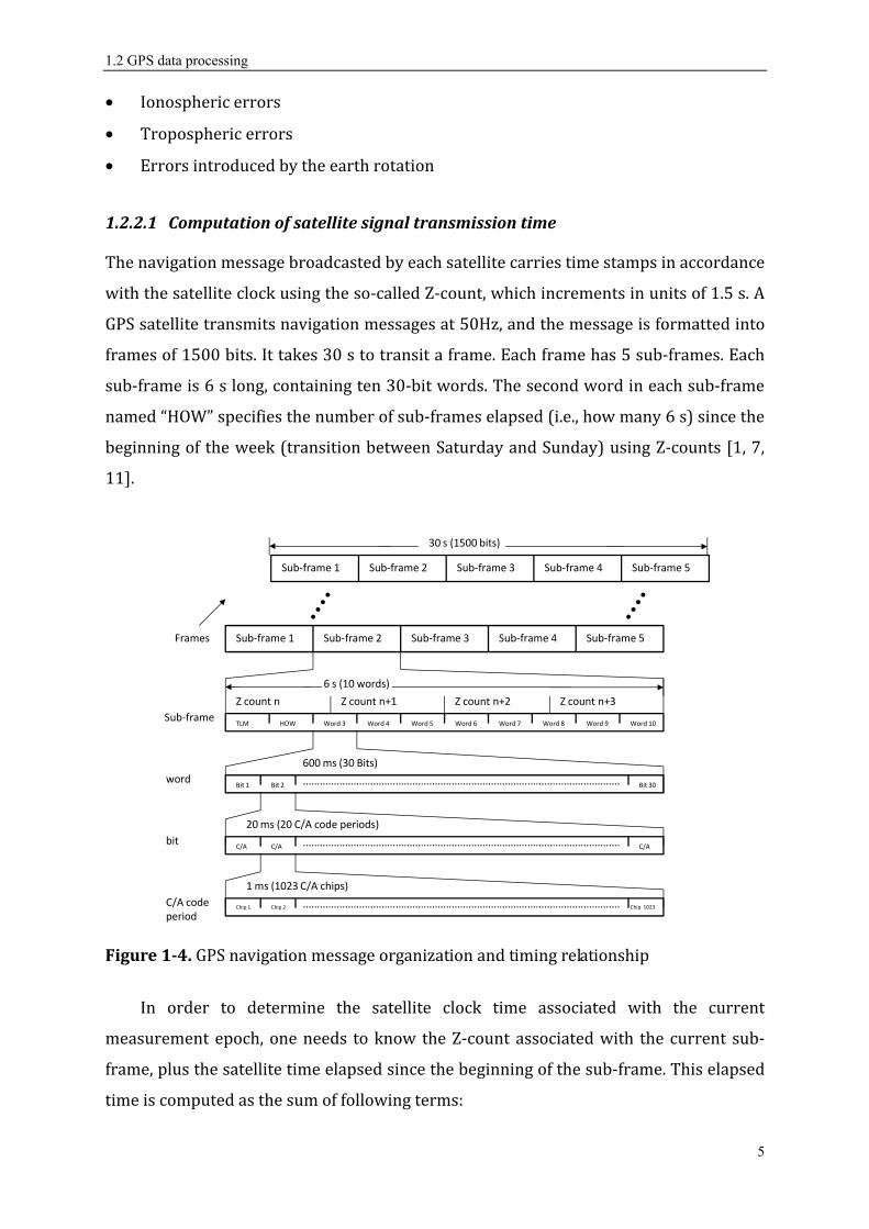
• Ionospheric errors • Tropospheric errors • Errors introduced by the earth rotation 1.2.2.1 Computation of satellite signal transmission time The navigation message broadcasted by each satellite carries time stamps in accordance with the satellite clock using the so-called Z-count, which increments in units of 1.5 s. A GPS satellite transmits navigation messages at 50Hz, and the message is formatted into frames of 1500 bits. It takes 30 s to transit a frame. Each frame has 5 sub-frames. Each sub-frame is 6 s long, containing ten 30-bit words. The second word in each sub-frame named “HOW” specifies the number of sub-frames elapsed (i.e., how many 6 s) since the beginning of the week (transition between Saturday and Sunday) using Z-counts [1, 7, 11].
Frames
Sub-frame 1 Sub-frame 3 Sub-frame 4 Sub-frame 5Sub-frame 2
Sub-frame 1 Sub-frame 3 Sub-frame 4 Sub-frame 5Sub-frame 2
30 s (1500 bits)
6 s (10 words)
Sub-frameTLM HOW Word 3 Word 4 Word 5 Word 6 Word 7 Word 8 Word 9 Word 10
Z count n Z count n+1 Z count n+2 Z count n+3
Bit 1 Bit 30Bit 2
C/A C/AC/A
600 ms (30 Bits)
20 ms (20 C/A code periods)
Chip 1
1 ms (1023 C/A chips)
Chip 2 Chip 1023
word
bit
C/A codeperiod
Figure 1-4. GPS navigation message organization and timing relationship In order to determine the satellite clock time associated with the current measurement epoch, one needs to know the Z-count associated with the current sub-frame, plus the satellite time elapsed since the beginning of the sub-frame. This elapsed time is computed as the sum of following terms:

1.2 GPS data processing
6
1. Number of navigation message data bits transmitted in the current sub-frame 2. Number of C/A code periods since the beginning of the current message bit 3. Number of whole chips in the current C/A-code cycle 4. The fraction of the current C/A-code chip The 1 and 2 are counted by the receiver software. The remaining two terms are provided by the receiver delay lock loop (DLL) though correlation process. The timing relationship between the satellite signal transmission time, receiver signal reception time, clocks offsets and pseudorange time equivalent are illustrated in Figure 1-5. That is, the satellite signal transmission time is equal to subtracting the ideal pseudorange divided by speed of light from the receiver’s time-tag for the measurement, and compensating clock bias terms.
sT uT
tΔ
Geometric range time equivalent
Pseudorange time equivalent
utst
s sT t+ u uT t+
Figure 1-5. Pseudorange measurement timing relationship This timing relationship can be formulated in Equation (1.2).
( )s u u sT T t tc
ρ= − − + (1.2)
where: sT Satellite signal transmission timeuT Receiver signal reception timest Offset of satellite clock from GPS reference timeut Offset of receiver clock from GPS reference times sT t+ Satellite clock reading at the time of signal transmissionu uT t+ Receiver clock reading at the time the signal receptionc Speed of light

1.2 GPS data processing
7
1.2.2.2 Computation of satellite clock correction The satellites contain atomic clocks that control on-board timing operations. The master control segment (MCS) consistently determines and transmits clock correction parameters to the satellites for rebroadcast in the navigation message. The correction parameter is made by the receiver using a second-order polynomial [7]: 2
20 1 2
2
sin
( ) ( )
r k
s f f s oc f s oc r
F c
t Fe a E
t a a T t a T t t
μ= −
Δ =
= + − + − + Δ
(1.3)where:
:kE Eccentric anomaly of the satellite orbit :rtΔ Correction due to the relativistic effects
0 :fa Clock bias parameter 1 :fa Clock drift parameter 2 :fa Frequency drift parameter :oct Ephemeris clock data reference time :sT Signal transmission time The satellite group delays are initially calculated by the master control segment, and the values for each satellite are updated to reflect the actual on-orbit group delay. These values are given in the navigation data message. Therefore, corrections can be directly applied as:
gds s gdt t T= − (1.4)
where gdT The group delay of the satellite expressed in seconds gdst Satellite clock offset with group delay compensated
1.2.2.3 Computation of satellite position based on ephemeris orbital parameters The ability to accurately predict the position of a satellite at the instant of signal transmission is vital to the operation of GPS. The satellite position can be computed in Earth-Centered, Earth-Fixed (ECEF) coordinate at its time of transmission using the broadcasted ephemeris orbital data. The ephemeris parameters describe the orbit of the space vehicle, and provide the best trajectory fit for each specific fit interval. The orbital

1.2 GPS data processing
8
parameters using Keplerian orbital parameters are given in Table 1-1. Constant parameters are given in Table 1-2. And the computation of satellite position at signal transmission time is shown in Table 1-3. A detailed explanation can also be found in [1, 7]. Table 1-1. Ephemeris orbital data Data Physical meanings
0M Mean Anomaly at Reference Time nΔ Mean Motion Difference From Computed Value e Eccentricity a Square Root of the Semi-Major Axis 0Ω Longitude of Ascending Node of Orbit Plane at Weekly Epoch
0i Inclination Angle at Reference Time ω Argument of Perigee Ω Rate of Right Ascension di dt Rate of Inclination Angle
ucC Amplitude of the Cosine Harmonic Correction Term to the Argument of Latitude usC Amplitude of the Sine Harmonic Correction Term to the Argument of Latitude rcC Amplitude of the Cosine Harmonic Correction Term to the Orbit Radius rsC Amplitude of the Sine Harmonic Correction Term to the Orbit Radius icC Amplitude of the Cosine Harmonic Correction Term to the Angle of Inclination isC Amplitude of the Sine Harmonic Correction Term to the Angle of Inclination oet Reference Time Ephemeris
Table 1-2. Constant parameters Constant parameters Physical meanings 143.986005 10μ = × m3/s2 Earth universal gravitational parameter (WGS 84)
57.2921151467 10e−Ω = × rad/s Earth rotation rate (WGS 84)
82.99792458 10c = × m/s Speed of light

1.2 GPS data processing
9
Table 1-3. Calculation of satellite position using ephemeris orbital data Computations Physical meanings of computations1) ( )2
a a= Semi-major axis 2) 0 3n
a
μ= Computed mean motion (rad/sec) 3) k s oet T t= − Time from ephemeris reference epoch 4) 0n n n= + Δ Corrected mean motion 5) 0 kk tM M n= + Mean anomaly 6)
1 2
131
1 2 2
2
; ; 1; 0;
10
sin ;
; ; 1;
10, ,
k k k k
k k k
k k
E M E E f f
while f
E M e E
f E E E E f f
if f break end
end
−
′= = = = > = + ′ ′ = − = = + >
Kepler’s Equation for Eccentric Anomaly (must be solved iteratively for kE ). 7) ( )
21 1 sin (1 cos )
tancos (1 cos )
k kk
k k
e E e Ev
E e e E− − − = − −
True Anomaly 8) 1 cos
cos1 cos
kk
k
e vE
e v− += +
Eccentric Anomaly 9) k kv ωΦ = + Argument of Latitude 10) sin 2 cos 2
sin 2 cos 2
sin 2 cos 2
k us k uc k
k rs k rc k
k is k ic k
u C C
r C C
i C C
δδδ
= Φ + Φ = Φ + Φ = Φ + Φ
Argument of Latitude Correction Radius Correction Inclination Correction 11) k k ku uδ= Φ + Corrected Argument of Latitude 12) ( )1 cosk k kr a e E rδ= − + Corrected Radius 13) ( )0k k ki i i di dt tδ= + + Corrected Inclination 14) cos
sink k k
k k k
x r u
y r u
′ = ′ =
Positions in orbital plane 15) 0 ( )k e k e oet tΩ = Ω + Ω − Ω − Ω Corrected longitude of ascending node 16) cos cos sin
sin cos cos
sin
k k k k k k
k k k k k k
k k k
x x y i
y x y i
z y i
′ ′= Ω − Ω ′ ′= Ω + Ω ′=
Satellite position in ECEF frame

1.2 GPS data processing
10
1.2.2.4 Computation of the ionospheric error In this dissertation, the ionospheric delay corrections are computed from the broadcasted model parameters in the navigation message according to GPS-ICD-200 [7]. It is estimated that the use of this model will provide at least a 50 percent reduction in the single-frequency user’s root mean square (RMS) error due to ionospheric propagation effects [1, 7]. Table 1-4. Computation of ionospheric correction Computations 1) /E el π= 2) 31.0 16[0.53 ]F E= + − 3) 0.0137
0.0220.11E
ψ = −+
4) 0.416, cos ;
0.416, 0.416;
0.416, 0.416;
i i u
i i
i i
if A
if
if
φ φ φ ψφ φφ φ
≤ = + > = < − = −
5) sin
cosi ui
Aψλ λφ
= + 6) 0.064cos( 1.617)m i iφ φ λ= + − 7) 44.32 10 it GPStimeλ= × + 8) 86400, 86400;
0, 86400;
if t t t
if t t t
≥ = −< = +
9) 2 3
1 2 3 472000, ;
72000, 72000;m m mif PER PER
if PER PER
β β φ β φ β φ ≥ = + + +
< =
10) 2 ( 50400)tx
PER
π −= 11) 2 3
1 2 3 40, ;
0, 0;m m mif AMP AMP
if AMP AMP
α α φ α φ α φ ≥ = + + +
< =
12) 2 49
9
1.57, 5 10 1 ;2 24
1.57, 5 10 ;
iono
iono
x xf x T F AMP
if x T F
−
−
< = × + − +
≥ = ∗ ×
where nα The coefficients of a cubic equation representing the amplitude of the vertical delay nβ The coefficient of a cubic equation representing the period of the model

1.2 GPS data processing
11
E Elevation angle between the user and satellite in semi-circles A Azimuth angle between the user and satellite, measured clockwise positive from the true North in semi-circles uφ User geodetic latitude in semi-circles (WGS-84) uλ User geodetic longitude in semi-circles (WGS-84) x Phase in radians t local time mφ Geomagnetic latitude of the earth projection of the ionospheric intersection point iλ Geodetic longitude of the earth projection of the ionospheric intersection point iφ Geodetic latitude of the earth projection of the ionospheric intersection point
ψ Earth’s central angle between the user position and the earth projection of ionospheric intersection point 1.2.2.5 Computation of the tropospheric errors The tropospheric error is often modeled as including both a dry (hydrostatic) and wet (non-hydrostatic) components. The dry component, which arises from the dry air, gives rise to about 90% of the tropospheric delay and can be predicted accurately [9-11]. The wet component, which arises from the water vapor, is more difficult to be predicted due to uncertainties in the atmospheric distribution (e.g., based on local weather condition and may change dramatically over time). The approach to cope with dry delay is usually handed by computing its delay in zenith direction (e.g., using Hopfield model), with a map function for considering the elevation angle [9, 10], as shown in Equation (1.5).
[ ]2
1 6 77.64 /40136 148.72( 273.16)
5 sin 6.25tropo
e p TT T
el
− ⋅= ⋅ ⋅ − −+ (1.5)
where “el” is the elevation angle; “p” is the atmospheric pressure in millibar (mb) and “T” is the temperature in Kelvin. As shown in Equation (1.5), in order to accurately compute the dry delay, the accurate local surface temperature and pressure measurements should be given. However, for navigation applications, such information may not always be available. Thus, a simplified model can be used (derived empirically) as: 2.47
sin( ) 0.0121tropoTel
=+ (1.6)
The estimated tropospheric dry delay with respect to different elevation angles (i.e., from 1 deg to 90 deg) are compared using Equation (1.5) and (1.6). For Hopfield’s

1.2 GPS data processing
12
model, we consider “p” as standard atmosphere (i.e., 1013.25 mb), and temperature as 298.15 Kelvin (i.e., 25 Celsius). The computed dry delays are shown in Figure 1-6.
Figure 1-6: Tropospheric delay estimates comparison using different models As depicted in the figure, major differences appear when the elevation angle is smaller than 5 degrees. However, in the GPS data processing, usually a mask elevation angle (e.g., >10 deg) is introduced to avoid using the measurements from the satellite with very low elevation angle. These measurements are often heavily deteriorated by interferes (e.g., multipath effects). For large elevation angles, differences in the estimated dry delays are very small, e.g., 0.1 m at 90 deg elevation angle and 0.3 m with 10 deg elevation angle. 1.2.2.6 Errors introduced from earth rotation Due to the rotation of the earth during the time of signal transmission, a relativistic error is introduced, which is known as the Sagnac effect. That is, during the signal propagation period, the earth experiences a finite rotation with respect to an earth center inertial (ECI) coordinate system. If the satellite and receiver coordinates are expressed in ECEF frame, the earth rotation during the signal propagation cannot be taken into consideration (coordinate rotates with the earth). Therefore errors are introduced. One approach to avoid the Sagnac effect is to work within an ECI coordinate frame for satellite and user position computations. An ECI frame can be artificially obtained by

1.2 GPS data processing
13
freezing an ECEF frame at every time instant when the pseudorange measurements are made by the receiver to the set of visible satellites. At these time instances, the ECI and ECEF frames are overlapped. For computing the user positions, they are the same. However, the satellite coordinates in ECEF frame needs to be transformed into ECI considering the earth rotation during the signal propagation period. This transformation can be calculated in Equation (1.7). cos ( ) sin ( ) 0
sin ( ) cos ( ) 0
0 0 1
s u s u s s
s u s u s s
s sECI ECEF
x T T T T x
y T T T T y
z z
Ω − Ω − = − Ω − Ω −
(1.7)
The u sT T− can be calculated as the corrected pseudorange measurements divided by speed of light. After coordinate transformation, both satellite and receiver coordinates are expressed in the same frame. They are either in ECI or in ECEF, because these two coordinates are overlapped at the time instance, when measurements are made by the receiver [1]. 1.2.2.7 Multipath errors Multipath refers to the phenomenon of a signal reaching an antenna via two or more paths. Typically, one antenna receives the direct (i.e., line-of-sight) signal and one or more of its reflections from structures in the vicinity and from the ground. The subsequent pseudorange measurements are of the sum of all the received signals. The pseudorange measurement multipath error is based on the strength of the reflected signal and the delay between the direct and reflected signals. It is probably the dominant source of error in GPS-based high-precision applications since it can introduce a bias up to a hundred of meters when employing a 1-chip wide (standard) Delay Lock Loop (DLL) to track the PRN code [11]. The method to reduce the multipath effect is either to locate the antenna away from reflectors (not always practical), or improve the receiver antenna design and signal processing steps in tracking loops, which can be only achieved by the receiver manufactures. 1.2.3 Position determination using pseudorange measurements
In order to determine the user position and receiver clock offset, usually four pseudorange measurements are required, which relate the user position coordinates as:

1.2 GPS data processing
14
( ) ( ) ( )2 2 2( , , , )j u u u u j u j u j u uf x y z t x x y y z z ctρ = = − + − + − + (1.8)
The “j” represents the j-th satellite, and ( , , )j j jx y z denotes the j-th satellite’s position coordinates in ECEF. The true user position and receiver clock offset ( ux , uy , uz , ut ) are considered to include approximate components ( ˆux , ˆuy , ˆuz , ut ) and incremental components ( uxδ , uyδ , uzδ , utδ ) as: ˆ
ˆ
ˆ
ˆ
u u u
u u u
u u u
u u u
x x x
y y y
z z z
t t t
δδδ
δ
= −= −= −= −
(1.9)
Thus, equation (1.8) can be reformulated as: ˆˆ ˆ ˆ( , , , )
ˆ ˆˆ ˆ ˆ ˆˆ ˆ( , , , ) ( , , , )ˆˆ ˆ ˆ( , , , )ˆ ˆ
ˆ ˆˆ ˆ ˆ ˆˆ ˆ( , , , ) ( , , , ). .
ˆˆ
j u u u u
u u u u u u u uu u u u
u u
u u u u u u u u
u u
f x x y y z z t t
f x y z t f x y z tf x y z t x y
x y
f x y z t f x y z tz t h o t
z t
ρ δ δ δ δ
δ δ
δ δ
= − − − −
∂ ∂ = − −∂ ∂
∂ ∂ − − +∂ ∂
(1.10)
We denote satellite position vector as [ , , ]Tj j j jx y z=x , and the estimated receiver position vector as [ , , ]Tu u u ux y z=x . j u−x x represents the estimated satellite-to-user distance. The partial derivative parameters in Equation (1.10) can be computed as: ˆˆˆ ˆ ˆ( , , , )
ˆ
ˆˆˆ ˆ ˆ( , , , )ˆ
ˆ ˆˆ ˆ ˆ( , , , )
ˆ
ˆˆ ˆ ˆ( , , , )ˆ
j uu u u u
u j u
j uu u u u
u j u
j uu u u u
u j u
u u u u
u
x xf x y z t
x
y yf x y z t
y
z zf x y z t
z
f x y z tc
t
−∂ = −∂ −
−∂ = −∂ −
−∂ = −∂ −
∂ =∂
x x
x x
x x
(1.11)
We denote 1ˆ ˆ ˆ, ,
T
j j u j u j u
j u
x x y y z z = − − − −l
x x, which is the estimated line-of-sight
unit vector pointing from the initial estimate of the user position to the j-th satellite. By

1.2 GPS data processing
15
substituting ˆˆ ˆ ˆ ˆ( , , , )j u u u uf x y z tρ = in Equation (1.10) and ignoring the higher order terms (i.e., “h.o.t” in Equation (1.10)). For n pseudoranges, we have: ( )( )
( )
1 1 31 1
22 2 1 3
1 3
,1ˆ
ˆ ,1
ˆ ,1
T
uT
u
u
Tn n un
x
y
z
c t
ρ
ρ ρ δρ ρ δ
δρ ρ δ
×
×
×
− − − − Δ = = + − −
l
l
l
r ε
(1.12)
We define: ( )( )
( )
1 1 3
2 1 3
1 3
,1
,1,
,1
T
u T
u u
uTn
x
y
z
δδ δ
δ
×
×
×
− − = =
−
l
lp H
l
(1.13)
Thus, for 4 satellites in view, we can solve Equation (1.12) directly as: 1u
uc t
δδ
− = ⋅ Δ
pH r (1.14)
After obtaining the incremental components, we can update the estimates of user’s coordinates and clock offset using Equation (1.9). This process (i.e. from Equation (1.9) to (1.14)) should be reiterated until uδp is sufficiently small, which is decided by the user’s accuracy requirements. For more than four satellites available, a least-squares estimation technique can be applied. In this way, the incremental components are computed as: ( ) 1u T T
uc t
δδ
− = ⋅ Δ
pH H H r (1.15)
1.2.4 Doppler measurement model
The relative motion of a satellite and the user results in changes in the observed frequency of the satellite signal. Given the satellite velocity (dividing the difference of satellite positions from adjacent epochs by the time interval), the Doppler

1.2 GPS data processing
16
measurements can be used to estimate the user velocity. However, they are biased by the receiver clock drift errors. The Doppler measurement from one satellite at one time instance can be formulated as [11]: ( )u s iono tropoc t t T Tρ ρ= + − + + (1.16)
where ρ The measured user to satellite range rate ρ The true user to satellite range rate ut Receiver clock drift st Satellite clock drift ionoT Rate of change in ionospheric delay tropoT Rate of change in tropospheric delay The Doppler shift can also be written as a projection of the relative velocity vector on the satellite line-of-sight vector as [11]:
( ) ( )Ts
u s u uct ρρ ε= − + +l v v (1.17)
where sul User-to-satellite line-of-sight unit vector sv Satellite velocity vector (e.g., in ECEF frame) uv Receiver velocity vector (e.g., in ECEF frame) ρε Combined error due to changes during the measurement interval in the satellite clock, ionosphere, and troposphere.
1.2.5 Velocity determination using Doppler measurements
As shown in Equation (1.17), with the knowledge of user location, the following relationship exists for the j-th satellite: ( ) ( )T T
j j j j u uct ρρ ε− = − + +l v l v (1.18)
The quantities on the left side of Equation (1.18) are either measurement or already computed. The , , ,, ,T
j j x j y j z = v v v v from j-th satellite can be derived from ephemeris orbital data. Therefore, we can denote the left side of Equation (1.18) as jd , and Equation (1.18) is formulated as:

1.2 GPS data processing
17
( )Tj j u ud ct ρε= − + +l v (1.19)For n Doppler measurements, we have:
( )( )
( )
1 1 31 ,
22 ,1 3
,
1 3
, 1
, 1
, 1
, 1
T
u xT
u y
u z
Tn un
d v
d v
v
d ct
×
×
×
− − = = + −
l
ld
l
ρε (1.20)
Using the geometric matrix H , as introduced in Equation (1.13), when 4 satellites are in view, user velocity estimates are computed as: 1u
uct−
= ⋅
vH d (1.21)
For more than 4 satellites in view, the least-squares estimation method can be utilized. ( ) 1u T T
uct
− = ⋅
vH H H d (1.22)
Using error states, similar like in former section, we define the true user velocity and receiver clock drift ( ux , uy , uz , ut ) are considered to include approximate components ( ˆux , ˆ
uy , ˆuz , ˆ
ut ) and incremental components ( uxδ , uyδ , uzδ , utδ ) as: ˆ
ˆ
ˆ
ˆ
u u u
u u u
u u u
u u u
x x x
y y y
z z z
t t t
δ
δδ
δ
= −
= −
= −
= −
(1.23)
We denote [ ], ,T
u u u ux y z= v , ˆ ˆ ˆˆ , ,T
u u u ux y z = v and [ ], ,T
u u u ux y zδ δ δ δ= v . Thus, we have ˆu u uδ= −v v v . Substitute them into Equation (1.17) yields: ( ) ˆˆ( )
j
T
j j j u u u uct c t ρρ δ δ ε = − + + − +l v v v (1.24)
Rearranging Equation (1.24) as:

1.3 INS principle
18
( ) ( )ˆˆ( )j
T T
j j j u u j u uct c t ρρ δ δ ε − − + = − + l v v l v
(1.25) We denote ( ) ˆˆ ˆ( )
T
j j j u uctρ = − +l v v , and we have: ( )ˆ
j
T
j j j u uc t ρρ ρ δ δ ε− = − + +l v (1.26)
Thus, for n Doppler measurements, we have: ( )( )
( )
1 1 31 1
22 2 1 3
1 3
, 1ˆ
ˆ , 1
, 1ˆ , 1
T
uT
u
u
T un n n
x
y
z
c t
ρ ρ δδρ ρδδρ ρ
×
×
×
− − −− Δ = = + − −
l
lε
l
r ρ (1.27)
1.3 INS principle
Inertial navigation is based on Newtonian physics and is affected by gravity. That is, the object will remain in uniform motion unless disturbed by an external force. It involves a blend of inertial measurements, mathematics, control system design and geodesy [12]. The external force generates acceleration on the object, which can be measured by the inertial sensor. After integration of the measured accelerations, the change in velocity and position with respect to the initial conditions can be determined. A conventional inertial measurement unit (IMU) consists of three gyroscopes for measuring angular rates and three accelerometers for measuring accelerations. They are mounted in triads so that the sensitive axes of sensors are mutually orthogonal, setting up a Cartesian reference frame. For the accelerometer, it measures the total accelerations encountered by the object, and it cannot distinguish between the accelerations caused by gravity or by inertial motions. An accelerometer at rest relative to the surface of the earth will sense the force due to gravity and the centrifugal force caused by the earth’s rotation. A non-rotating accelerometer which is in free fall, accelerating at the rate of gravity, will sense nothing. Therefore, using an accelerometer, the user must compensate the specific force caused by gravity. In order to do so, the tilt of the platform, on which accelerometers are

1.3 INS principle
19
mounded in triad, with respect to the local vertical needs to be known. Therefore, in an IMU, gyroscopes are needed. The gyroscopes are used to measure the attitude. They measure the angular rates from the body frame to the inertial frame. After integration, the changes in angle with respect to an initial condition can be determined. Figure 1-7 is a photograph showing the size of an MEMS-based IMU (LandmarkTM20 eXT). The mounting of this IMU in field experiments is shown in Figure 1-8.
Figure 1-7. LandmarkTM20 eXT MEMS-based IMU
Figure 1-8. Tri-axial IMU aligned in the vehicle body frame The IMU coordinate is usually aligned with the vehicle body frame coordinate, where the sensor x-axis often points to the forward direction, the y-axis points to the lateral direction, and the z-axis points to the vertical down direction forming a right-handed orthogonal coordinate (e.g., for LandmarkTM20 eXT). Different IMUs may use different coordinates.
1.3.1 INS strapdown mechanizations
For strapdown inertial sensors, the inertial sensor assembly is mounted directly on the vehicle platform. The sensor raw data are processed to yield navigation solutions (i.e., position, velocity, and attitude), and this process is named strapdown processing. A system that contains an IMU and a processing unit for computing navigation solutions is called an inertial navigation system (INS).

1.3 INS principle
20
1.3.1.1 Inertial frame mechanization For navigation in the vicinity of Earth, we usually derive the position, velocity and attitude estimates of the vehicle with respect to an Earth-fixed frame. However, due to the rotation of the Earth, additional apparent forces will be acting which are functions of the reference frame motion (i.e., theorem of Coriolis). Thus, the inertial velocity of vehicle iv can be computed from its ground velocity with respect to earth ev plus the Coriolis term ie ×ω r , owning to the earth rotation. i e ie= + ×v v ω r (1.28)where r is the position vector of the vehicle with respect to the origin of the reference frame (i.e., center of earth); “×” denotes a vector cross product; ieω represents the turn rate of the earth frame with respect to the inertial frame. Differentiating Equation (1.28) with respect to inertial frame yields:
i e ie iei ii
d
dt= + × + × r
v v ω r ω (1.29) In Equation (1.29), the iv represents the acceleration encountered by the vehicle with respect to the inertial frame. It equals to the sum of specific forces measured by the accelerometers and the force caused by the mass attraction gravitation (i.e., i = +v f g ). The
i
d
dt
r denotes the derivative of the position vector of the vehicle with respect to the origin of the inertial reference frame, which equals to iv . By substituting Equation (1.28) into (1.29), and assuming the earth rotation rate to be constant 0ie i
=ω , we arrive at: ( )e ie e ie iei
= − × + − × × v f ω v g ω ω r (1.30) Equation (1.30) shows that, the acceleration encountered by the vehicle with respect to Earth expressed in inertial axes is equal to the specific force measured by the accelerometers f compensated for the Coriolis acceleration ie e×ω v (due to the velocity of the vehicle over a rotating Earth) plus the local gravitational acceleration, which arises through mass attraction g and the centripetal acceleration ( )ie ie× ×ω ω r owning to the rotation of the earth.

1.3 INS principle
21
1.3.1.2 Navigation frame mechanization A navigation frame is often used for travelling around the Earth, where coordinates are defined in terms of north, east and down directions. For applications which cover large distances around the Earth, the rotation of the navigation frame with respect to the Earth-fixed frame (i.e., transport rate) needs to be considered. The vehicle navigation equations with respect to the navigation axes can be computed from the inertial frame mechanization equation (Equation (1.30)). That is, the ground acceleration of the vehicle expressed in the navigation frame is equal to the ground acceleration expressed in the inertial frame compensated the Coriolis terms encountered by the rotations of the navigation frame with respect to the Earth-fixed frame, and the Earth-fixed frame with respect to the inertial frame. This relationship is given in Equation (1.31). ( )e e ie en en i
= − + ×v v ω ω v (1.31) Substituting e i
v from Equation (1.30), and expressing all the terms in navigation axes yields: ( )
( )( )
(2 )
n n n n n n n n n ne ie e ie ie ie en e
n b n n n n n nb ib ie en e ie ie
= − × + − × × − + ×
= − + × + − × ×
v f ω v g ω ω r ω ω v
R f ω ω v g ω ω r
(1.32)where superscript “n” denotes that the quantities are expressed in the navigation frame;
nbR is the direction cosine matrix used to transform the measured specific force vector into navigation axes, and b
ibf represents the specific force measured by a perfect triad accelerometers mounted on the vehicle body frame. The second term on the right side is a correction caused by the Coriolis acceleration due to vehicle’s velocity over the surface of a rotating Earth. The third term is the apparent gravitational force acting on the vehicle. The fourth term represents the centripetal force owning to the rotation rate of the Earth. For low-cost MEMS-based IMU and short distance navigation applications, simplifications can be made to the navigation frame mechanization model. That is, when the gyroscope errors are significantly in excess of the rotation rate of the Earth, and the accelerometer bias errors are much larger than the centripetal forces introduced by the earth rotation, we can assume nie =ω 0 . Besides, for short distance navigation applications, the rotation of the navigation frame with respect to the Earth-fixed frame

1.3 INS principle
22
does not need to be considered. Then we will have nen =ω 0 . Taking these two aspects in consideration, Equation (1.32) can be simplified as:
n n b ne b ib= +v R f g (1.33)
The rotation rate of body frame with respect to navigation frame can be related with gyroscope angular rate raw measurements as: ( )
b b bnb ib in
b b n nib n ie en
= −
= − +
ω ω ω
ω R ω ω (1.34)where b
ibω is the angular rate measured by the body-mounted gyroscopes; binω represents the summing rotation rates of the Earth with respect to the inertial frame plus the turn rate of navigation frame with respect to the Earth. With ignoring the Earth rotation rate and transport rate (i.e., ( )n n
ie en+ =ω ω 0 ), the following relationship exists for connecting the derivative of Euler angles , ,
Tα β γ = Ψ and gyroscope angular rate measurements [13] as:
( )
n bb nb
n b b n nb ib n ie en
n bb ib
= ⋅
= − + = ⋅
Ψ E ω
E ω R ω ω
E ω
(1.35) with
1
0
0 / /
nb
S T C T
C S
S C C C
α β α βα α
α β α β
= −
E (1.36) where ,CX SX and TX represent the trigonometric operations of cosine, sine and tangent of X. The , ,α β γ denote the roll, pitch and yaw respectively. Having the derivative of Euler angles and initial attitude information, we can compute the attitude estimates (e.g., Euler angles) by using integral operations. And the body frame to navigation frame direction cosine matrix n
bR can be formulated, as shown in Equation (1.37).

1.3 INS principle
23
It is the transpose of bnR , which is formed by the rotation sequence of Z-Y-X from the navigation frame to the body frame. It is worth mentioning that, different sequence of rotations yields a different presentation of direction cosine matrix.
nb
C C C S S S C C S C S S
S C S S S C C S S C C S
S C S C C
γ β γ β α γ α γ β α γ αγ β γ β α γ α γ β α γ α
β β α β α
− + = + − −
R (1.37)From Equation (1.33) to (1.37), we can form the INS strapdown process model for the low-cost MEMS-based IMU in discrete time domain as:
( )1
1 , ,
1 , ,
n n nk k k
n n n b nk k b k ib k
n bk k b k ib k
t
t
t
+
+
+
= + ⋅ Δ
= + ⋅ + ⋅ Δ
= + ⋅ ⋅ Δ
p p v
v v R f g
Ψ Ψ E ω
(1.38)where k is the time instant; ,
bib kf is the ideal triad accelerometer measurement vector;
,bib kω represents the ideal triad gyroscope measurement vector; ng is the gravity vector without considering the local centripetal forces; kΨ is the Euler angles; ,
nb kR is the frame rotation matrix from body frame to north east and down (NED) navigation frame, and
,nb kE is the rotation rate transformation matrix between body and navigation frame. A flow-chart of the general strapdown mechanization process in navigation frame for all levels of inertial sensors (i.e. without simplifications) is depicted in Figure 1-9.

1.4 INS/GPS integration
24
3 accel.
3 gyro.
bibf
bibω Attitude
computation
ψ Forming
,n nb bR E
nbE
PositionVelocitySolutions
nbR
Initial attitudeinformation
nibfTrans. to
n-frame
nVCorioliscorrection
Gravity computation
Initial position and velocityinformation
nP
nlg
Local gravity vector
Earth rateTransport rate
Positionvelocity
,n nie enω ω
nieω
_
++
+
Attitude
IMU
Figure 1-9. Strapdown mechanization in navigation frame.
1.4 INS/GPS integration
The GPS receiver offers long-term stable absolute positioning information with output rate at around 1 to 10 Hz. However, the system performance depends on the signal environment. It provides navigation solutions usually when more than four satellites are in view. In an INS, angular rate and specific force measurements from the IMU are processed to yield position, velocity and attitude solutions. Such systems can act autonomously and provide measurements at a higher data rate (e.g., 100 Hz). However, similar as other dead reckoning sensor systems, in an INS, the IMU sensor errors, such as sensor bias, scale factor error and noise will cause an accumulation in navigation solution errors over time. For example, the tilt errors caused by the integration of gyroscope sensor errors blur the distinction between the acceleration measured by the vehicles motion and that due to the gravity, which yields inaccurate velocity and position solutions. An integrated INS/GPS system combines the advantages of both sides and can provide accurate and uninterrupted navigation results. In such an integration system, the GPS data is used to provide absolute positioning information for frequently updating the INS estimates. And the INS data is used to provide the short-term solutions during GPS outage signal environments.

1.4 INS/GPS integration
25
The primary methods used to fuse the INS and GPS data are the loosely-coupled or tightly-coupled integration. For the deeply-coupled (or ultra-tightly coupled) integration, the GPS receiver tracking loops need to be accessed, which is usually not provided by hardware manufacturers. Therefore, in this dissertation, it will not be discussed. 1.4.1 Loosely-coupled integration
The loosely-coupled integration has a decentralized estimation architecture, which uses the output information of the navigation solutions from a GPS receiver and an INS. One example using error states is given in Figure 1-10, where INS and GPS estimates (i.e., position and velocity) are compared, the resulting differences forming the measurement input to the integration Kalman filter. The filter yields estimates of the inertial sensor errors, which will be used to compensate the inertial sensor measurements. Besides, the compensation of estimated navigation solution errors from the INS estimated solution should be conducted after every Kalman filter measurement update.
3 gyro.3 accel.
,b bib ibf ω
GPS receiver1-12channels GPS
navigation processing
,ρ ρ
IMUINSStrapdownprocessing
ˆ ˆ ˆ, ,P V A
,P V Integration Kalman filtering
ˆ ˆ ˆδ ,δ ,δP V A
Δ Δ,P V
ˆ ˆ ˆ, ,P V A
_
+
+
_
+
_
δ δˆ ˆ,b bib ibf ω
Figure 1-10. INS/GPS Loosely-coupled integration (indirect feedback) The main advantages of using loosely-coupled integration can be summarized as: The system observation model is simpler with respect to that in tightly-coupled manner, and accordingly it requires much less computational burden in the integration KF.

1.4 INS/GPS integration
26
The number of measurement input for the Kalman filter is fixed (i.e. position and velocity). Redundant GPS navigation solutions are available. The disadvantages can be summarized as: In case of using two separate KFs (i.e., one for GPS navigation processing, and the other for integration purpose), it opens the possibility of presenting instable navigation solutions caused by mutual feedbacks of estimation errors, which is coined as cascaded filtering problem. Usually more than 4 satellites are required to form and maintain a GPS navigation solution. For improving the system estimation accuracy, the integration KF can take advantage of covariance information from the GPS navigation processor outputs, which vary with satellite geometry. However, for many GPS receivers, these covariance data are simply not available. 1.4.2 Tightly-coupled integration
3 gyro.3 accel.
,b bib ibf ω
GPS receiver1-12channels ,ρ ρ
IMUINSStrapdownprocessing
ˆ ˆ ˆ, ,P V A
Integration Kalman filtering
ˆ ˆ ˆδ ,δ ,δP V A δ δˆ ˆ,b b
ib ibf ω
ˆ ˆ ˆ, ,P V A
_
+
+
_
+
_Predict ˆ,ρ ρ
Δ Δ ,ρ ρ
Figure 1-11. INS/GPS Tightly-coupled integration (indirect feedback) In tightly-coupled integration, only a centralized KF is used, and the pseudorange and delta range (Doppler) measurements are directly used in the filter as shown in Figure 1-11. In such a case, the GPS pseudorange and delta range measurements are compared with predicted quantities made by the inertial system. The differences form

1.4 INS/GPS integration
27
the measurement input to the integration KF to generate estimates of the INS navigation errors and sensor errors, which are used to correct the inertial system estimates after each measurement update. The corrected INS navigation solution forms the integrated navigation solution. The advantages of applying the tightly-coupled integration with respect to the loosely-coupled manner are mainly in the following aspects: The cascaded filtering problem arising through the mutual feedbacks of the estimation errors between two separate KFs is eliminated. The system does not require a GPS navigation solution to aid the INS. Even less than 4 satellites in view, the remaining satellite measurements can still be used in the algorithm, which promote the robustness of the navigation system. All systematic errors and noise sources of the distributed sensors are modeled in the same filter, which ensures that all error correlations are accounted for. The disadvantage of this method arises in the increased dimension of the observation vector. And the number of GPS measurements as input for the KF is varying during the navigation applications, which bases on the signal environments. 1.4.3 INS/GPS state space models using error states
In the integration of measurements coming from a single GPS receiver antenna and an INS without redundant attitude information (e.g., from magnetometers, or multi-antenna GPS systems), the INS attitude (i.e., heading) and sensor bias errors are weakly observable, which are based on the dynamics of the platform [14-17]. They are essentially corrected by the GPS updates through the off-diagonal parameters in their error covariance matrices in the filter. It is the nonlinear system model that relates the attitude errors, sensor bias errors with the position and velocity errors. Therefore, the nonlinearity of the INS/GPS integrated system model should be carefully treated. The most common application of the KF to nonlinear systems is the extended Kalman filter (EKF), which will be used in this chapter. 1.4.3.1 System process model based on the first-order linearization In this section, we derive the models from the first-order linearization of nonlinear equations. The nonlinear system dynamic equations in navigation frame for low-cost MEMS-based IMU are given in Equation (1.39).

1.4 INS/GPS integration
28
1
1 , ,
1 , ,
, ,, 1 , ,
, ,, 1 , ,
ˆ
ˆ
n n nk k k
n n n b nk k b k ib k
n bk k b k ib k
b error b errorib k ib k k
b error b errorib k ib k k
t
t
t
+
+
+
+
+
= + ⋅ Δ
= + ⋅ + ⋅ Δ = + ⋅ ⋅ Δ
= +
= +f
ω
p p v
v v R f g
Ψ Ψ E
f f w
ω ω w
ω (1.39)
where 1nk+p denotes position in navigation frame at epoch k+1; 1
nk+v is the velocity in navigation frame at epoch k+1; 1k+Ψ is the attitude which includes roll, pitch and yaw estimates at epoch k+1; ,
, 1b errorib k+f and ,
, 1b errorib k+ω are the accelerometer and gyroscope sensor errors at epoch k+1, expressed in body frame. Here we define ,
, , ,ˆb b b errorib k ib k ib k= −f f f and ,
, , ,ˆ b b b errorib k ib k ib k= −ω ωω . The linearization is conducted at local (i.e., k-th epoch) estimated position, velocity, attitude, accelerometer and gyroscope sensor errors. The results are given in Equation (1.40). The error states are formed from the linearization process.
3 3 3 3 3 3 3 3 3 31
3 3 3 3 23, , 3 31
3 3 3 3 33, 3 3 ,1,
3 3 3 3 3 3 3 3 3 3, 1,
3 3 3 3 3 3 3 3 3 3, 1
n nk k
nnk b kk k
nk b kk
b errorib kb errorib k
t
t
t
× × × × ×+
× × ×+
× × ×+
× × × × ×+
× × × × ×+
Δ − Δ = − Δ ⋅
I I O O Op p
O I F R Ov v
O O F O EΨ
O O O I Of
O O O O Iω
δ δδ δδδδ
,,,,
n
kkb errorib kb errorib k
+
wΨ
f
ω
δδδ
(1.40)
where ,nb kR and ,
nb kE are the transformation matrices shown in Equation (1.36) and (1.37) at the time instance k. The sub-matrices 23,kF and 33,kF are computed in Equation (1.41) and (1.42).

1.4 INS/GPS integration
29
23,
ˆ ˆ ( )ˆ ( ) ˆ ˆ ( )
ˆ ( ) ˆ ˆ
ˆ ˆ ( )ˆ ( ) ˆ ˆ (ˆ ( ) ˆ
z z
y
x y
zy x
z z
z
k x y
y
y
f C C C f C S C S Sf S S C C S
f C S f C C S S Sf C S C S S
f C C S f C S
f C C S f S S C C Sf S S S C C
f S S f C S C S Sf C S C S S
f C S S
β α γ γ α α β γα γ α γ β
γ β α γ β α γα γ γ β α
β γ α β γ
β α γ α γ α γ ββ α γ α γ
β γ α γ γ β αγ α α β γ
β α γ
++
− − −+ +
+ −
+− +
= − − −− −
+
F
3 3
)
ˆ
ˆ
ˆ ˆ ˆ 0
ˆ
x
x
y z z
y
t
f C C
f C
f C C f C S f C S
f S S
β γ
β
β α β α α β
β α×
⋅Δ
+ − − − −
(1.41)
and
2
2
33,
2
3 3
ˆ ˆ ( 1)1 0
ˆˆ ( 1)
ˆ1 0
ˆ
ˆ ˆ ˆ ˆ1
y z
yz
z
ky
y z z y
C T C Tt t
S TT S
Ct
S
C S C S S St t
C C
ω α β ω α βω α βω β α
ω αω α
ω α ω α α βω β αωβ β
×
+ + Δ Δ + ++
= − Δ +
− + Δ Δ
F (1.42)
where 2 2,C X T X represent the square of cosine and tangent operations of X, and ,
, ,ˆ b b errorx ib x ib xf f f= − , ,
, ,ˆ b b errory ib y ib yf f f= − , ,
, ,ˆ b b errorz ib z ib zf f f= − , ,
, ,ˆ b b errory ib y ib y= −ω ω ω ,
,, ,ˆ b b error
z ib z ib z= −ω ω ω are the IMU raw data compensated with the estimated sensor errors at time instance k. Equation (1.40) can be used as the system process model for the loosely-coupled INS/GPS integration. However, for the tightly-coupled approach, the receiver clock bias and clock drift errors need to be modeled. We form the system process model for tightly-coupled integration in Equation (1.43), where the range-rate equivalent of the clock drift error is modeled as a constant plus a random walk process, while the range equivalent of the receiver clock bias error is the integral of the clock drift error.

1.4 INS/GPS integration
30
1 3 3 3 3 3 3 3 3 3 3 3 1 3 1
1 3 3 3 3 23, , 3 3 3 1 3 1
1 3 3 3 3 33, 3 3 , 3 1 3 1,, 1 3 3 3 3 3 3 3 3 3
,, 1
1
1
nkn nk k b k
nk k b k
b errorib k
b errorib k
k
k
t
t
t
c t
c t
+ × × × × × × ×
+ × × × × ×
+ × × × × ×
+ × × × × ×
+
+
+
Δ
− Δ − Δ
=
p I I O O O 0 0
v O I F R O 0 0
Ψ O O F O E 0 0
f O O O I O
ω
δδδδ
δ
δδ
,,3 3 1 3 1
,3 3 3 3 3 3 3 3 3 3 3 1 3 1 ,
3 1 3 1 3 1 3 1 3 1
3 1 3 1 3 1 3 1 3 1
1
0 1
nknk
kb errorib k k
b errorib k
T T T T T
kT T T T T
k
t c t
c t
× ×
× × × × × × ×
× × × × ×
× × × × ×
⋅ +
Δ
p
v
Ψ
f0 0 w
O O O O I 0 0 ω
0 0 0 0 0
0 0 0 0 0
δδδ
δ
δ
δδ
(1.43)
1.4.3.2 Observation model for loosely-coupled and tightly-coupled integration For the loosely-coupled integration, the position and velocity measurements from the GPS receiver are compared with the INS estimated quantities, forming the new measurement input for the integration KF. Its observation model is given as: 3 3 3 3 3 3 3 3 3 3
3 3 3 3 3 3 3 3 3 3 ,6 15,,,
ˆ
ˆ
nkn
n n kk kn nk kkk k b error
ib kb errorib k
× × × × ×
× × × × × ×
− = = ⋅ + −
p
vI O O O Op p
y εΨO I O O Ov v
f
ω
δδδ
δδ
(1.44)
In the tightly-coupled integration, the system observation model is formulated in Equation (1.45), which is the combination of Equation (1.12) and (1.27) introduced in former sections. ( )
( )( )
( )
1, 3 1 3 1 3 1 3 11 31, 1,
, , , 3 1 3 1 3 1 3 11 3
1, 1, 3 1 1, 3 1 3 1 3 11 3
, ,3 1 , 3 11 3
1 0ˆ
ˆ 1 0
ˆ0 1
ˆ
T T T T Tk
k k
T T T T Tj k j k j k
k T T T T Tk k k
T T Tj k j kj k
× × × ××
× × × ××
× × × ××
× ××
−− − − = =
− − − −
l 0 0 0 0
l 0 0 0 0y
0 l 0 0 0
0 l 0
ρ ρ
ρ ρ
ρ ρ
ρ ρ
,,
,,
3 1 3 12 17
0 1
nknk
kb errorib k k
b errorib k
kT T
kj
c t
c t× ××
⋅ +
p
v
Ψ
f ε
ω
0 0
δδδ
δ
δ
δδ
(1.45)
where ‘j’ denotes the number of satellites in view. By looking at the dimension of the observation matrix in Equation (1.44) and (1.45), we observe that in the tightly-coupled integration, the dimension of observation matrix varies during the time, which is based on the number of tracked satellites. If a large

1.5 Field experiment
31
number of satellites are in view, the observation matrix will be bulky and causes large computational burden. For instance, if 11 satellites are in view, the observation matrix has the dimension of 22x17. However, for the loosely-coupled integration, the dimension of the observation matrix is fixed (i.e., 6x15), which simplifies the implementation and reduces the computational burden. 1.5 Field experiment
In order to verify the algorithm from the INS/GPS integrated system, an experiment based on a train ride is made. We consider the tightly-coupled integration (due to its advantages as introduced in Section 1.4.2) as the approach to blend the INS and GPS data. The trajectory experienced frequent GPS outage environments (i.e., going through tunnels). The path starts from the city of Betzdorf to Siegen in the North West of Germany. The trajectory lasts 800 s, as shown in Figure 1-12. The number of tracked satellites is given in Figure 1-13.
Figure 1-12. A train ride trajectory computed from processing the L1 GPS pseudorange measurements using a least-squares estimation method (plotted in Google earth)

1.5 Field experiment
32
Figure 1-13. Number of satellites in view. One LandmarkTM20 eXT MEMS-based IMU (100 Hz) and one u-blox Antaris 4 (1 Hz) GPS receiver are used. The main sensor errors of the LandmarkTM20 eXT MEMS-based IMU are given in Table 1-5. Table 1-5. LandmarkTM20 eXT MEMS-based IMU performance specification. Gyroscope (Angular rates) Bias in-run stability Noise (ARW) Scale Factor Error20 [°/h] (1σ ) 0.035[°/s/√Hz] (1σ ) ≤ 1000 [ppm] Accelerometer (Specific forces) Bias in-run stability Noise (VRW) Scale Factor Error20 [µg] (1σ ) 40 [µg/√Hz] (1σ ) ≤ 1000 [ppm] The train went through tunnels 4 times during the trajectory. The durations of the GPS outage environments are given in Table 1-6. The system performances from tightly-coupled integration (blue curves) and GPS alone navigation solutions based on least-squares estimation method (red points) are depicted in Figure 1-14. In these periods, the INS bridges the GPS outages, and presents continuous and robust positioning results. Table 1-6. GPS outage environments GPS outages < 4 satellites in view no satellites in view a) 5 Seconds 2 Seconds b) 8 Seconds 5 Seconds c) 13 Seconds 9 Seconds d) 16 Seconds 9 Seconds Sum 42 Seconds 25 Seconds

1.5 Field experiment
33
a) GPS outage with 2 s (no Sat.), blue (integrated), red (GPS alone)
b) GPS outage with 5 s (no Sat.), blue (integrated), red (GPS alone)
c) GPS outage with 9 s (no Sat.), blue (integrated), red (GPS alone)

1.6 Summary
34
d) GPS outage with 9 s (no Sat.), blue (integrated), red (GPS alone) Figure 1-14. System performance comparison during tunnels (plotted in Google earth) Other than GPS outage environments, the multipath effects will significantly influence the GNSS positioning accuracy (e.g., caused by the elevated road and large building nearby, as shown in Figure 1-14 (d)). In this case, the INS estimates can smooth the noisy GNSS measurement so that the INS/GPS integrated solution presents a more accurate and robust navigation solution.
1.6 Summary
In this chapter, the GPS data processing, INS principles and INS strapdown processing have been introduced in detail. For the INS/GPS integration, the main advantages and disadvantages from the loosely-coupled and tightly-coupled integrations were discussed. The system process and observation models for both approaches were given. the model is derived from a first-order linearization process. One field experiment has been made based on a train ride to verify the advantage of INS/GPS integrated system with respect to GPS alone devices. Numerical results show that in GPS outage and highly reflective signal environments the integrated solution presents more accurate and robust navigation performance. In the following chapters, more advanced nonlinear filtering approaches will be applied on INS/GPS integration. Furthermore, quaternions will be employed as the representation of attitude, which does not exhibit the singularity problem.

2.1 Introduction
35
2. Nonlinear Filtering Methods
2.1 Introduction
“Filtering consists of recursively estimating and tracking of states governed by a linear or nonlinear stochastic system state space model based on a set of noisy observation data” [18]. Navigation is one of many areas, in which estimation theory can be successfully applied. In the navigation field, different methodologies will be used to estimate the time varying position, velocity and attitude of moving objects on the basis of measurements derived from navigation sensor systems [13]. In order to estimate the system dynamics recursively, one has to define a system propagation model, which describes the evolution of state over time, and an observation model, which relates the incoming measurements to the estimated states. In the Bayesian recursive estimation approach, all the states are regarded as random variables which can be completely described by their probability distributions. Thus, the estimation problem turns to be the recursive quantifying of the a posteriori state density function given all available observables. And hence, the conditional probability density functions of random variables will be of primary importance in following derivations. In the following sections, a few important basic concepts will be overviewed in the probability theory, and then the general recursive Bayesian filter will be introduced. The general recursive Bayesian filter provides a conceptual solution for nonlinear non-Gaussian applications. In order to apply it on INS/GPS integration, assumptions should be made, which leads to the UKF and PF algorithms. As one contribution of this thesis, a UPF algorithm is proposed, which combines the best of UKF and PF. A simulation test is made to show its merits with respect to other nonlinear filtering approaches.

2.2 Basics in probability theory
36
2.2 Basics in probability theory
Given a random variable vector 1 2[ , ,..... ]Tnx x x=x , the probability distribution function xF can be formulated as a scalar function of the dummy vector [ ]1 1, ,
T
nζ ζ ζ= ζ as: ( )( ) ( ) ( ){ }( )
1 2, , , 1 2
1 1 2 2
( ) , ,
: , , ,
nx x x n
n n
F F
P x x x
ζ ζ ζ
ω ω ζ ω ζ ω ζ
=
= ≤ ≤ ≤
x
ζ (2.1)where ω denotes the elementary outcome of the experiment in sample space; ( )ωx is the realization of the random variable mapping ω from sample space to real values in Euclidean space n ; ζ is a dummy vector consists of real values for integration; ( )P ⋅ is the probability function which assigns the probabilities to the event described in the parenthesis. It can be calculated as:
( )( )
1 2
1 2
1 2
, , , 1 2
, ,..... 1 2 1 2
( ) , , ,
, , ,
n
n
n
x x x n
x x x n n
F F
f d d dζ ζ ζ
ζ ζ ζ
ξ ξ ξ ξ ξ ξ−∞ −∞ −∞
=
= x
ζ (2.2)where [ ]1 2, , ,
T
nξ ξ ξξ = is a dummy vector for random variable x, which is used for integration. Equation (2.2) can be formulated in its vector expression for convenience as: ( )( )F f d
−∞= x x
ζζ ξ ξ (2.3)
where ( )fx ξ is called the probability density function. In the stochastic modeling and estimation, we often need to estimate the random variable vector x given the measurement vector y at its specific realization γ . The concept of the conditional expectation arises, which is calculated as: [ ] ( )|| |E f d
+∞
−∞= = ⋅ x yx y γ ξ ξ γ ξ (2.4)
Naturally, the expectation of certain functions of a random variable vector ( )g=z x on the basis of the measurement vector y at its specific realization of γ is formulated as:

2.2 Basics in probability theory
37
[ ] ( )|| ( ) |E g f d+∞
−∞= = ⋅ x yz y γ ξ ξ γ ξ (2.5)
For a Gaussian distributed random variable vector 1 2[ , ,..... ]Tnx x x=x , its probability density function is formulated as: ( )
( )[ ] [ ]1
1/2/2
1 1exp
22
T
nfπ
− = − − −
x x x x
x
m P mP
ξ ξ ξ (2.6)where xm and xP are the mean vector and covariance matrix of random variable vector x ; n is the dimension of the random variable vector; ⋅ denotes the determinant of a matrix, and { }exp ⋅ denotes the exponential function. Because the probability density function of a Gaussian random variable can be completely described by its mean and covariance parameters. Therefore, a shorthand notation is often used as:
( , )x xx m P (2.7) The joint probability density function of Gaussian random variable vectors 1 2[ , ,..... ]Tnx x x=x and 1 2[ , ,..... ]Tmy y y=y can be written as:
( )( )( )
1
, 1/2
/2
1 1exp
22
T
n m
f
π
−
+
− − = − − −
x xx xy x
x yy yx yy y
xx xy
yx yy
m P P m
m P P mP P
P P
ξ ξξ, γ γ γ (2.8)
where ξ and γ are dummy vectors which denote the realizations of random vectors x and y; , y xm m are their expectations respectively. According to Bayes’ rule, ( ) ( ) ( )| ,f | f f=x y x y yξ γ ξ, γ γ , the conditional density function ( )|f |x y ξ γ is computed as: ( )
( )1
| | | |1/2/2
|
1 1exp
22
T
nf
π− | = − − −
x y x y x y x y
x y
m P mP
ξ γ ξ ξ (2.9)where

2.3 Recursive Bayesian state estimator
38
( )|
|
= +
= −
-1x y x xy yy y
-1x y xx xy yy yx
m m P P m
P P P P P
γ − (2.10) In Equation (2.10), if we assume x represents the random variable vector of interest, and y denotes the new information coming from the external sensor measurements into the system. The ( )|fx y ξ | γ represents the conditional density for the random variable vector conditioned on the information obtained from the sensor output. If we assign 1−= xy yyK P P , we have:
( )|
|T
= +
= −x y x y
x y xx yy
m m K m
P P KP K
γ − (2.11) They are the Kalman filter equations derived from the conditional probability density function based on Gaussian distributions.
2.3 Recursive Bayesian state estimator
Linear systems do practically not really exist. They are approximations within a limited range in practical applications. For many problems, an estimate is required every time when a measurement is received. In this case, a recursive filter is a convenient solution. A recursive Bayesian approach to dynamic state estimation problems involves the construction of the probability function of the current state for an evolving system, given the accumulated observation history. It provides a rigorous general framework for dynamic state estimation problems [19]. In order to derive the recursive Bayesian equations, we assume that the discrete-time stochastic system state space models are as follows: 1 1 1( , )
( , )k k k k
k k k k
f
h− − −=
=x x w
y x v (2.12)where k is the time instant; kx is the system state vector; ky represents the measurement vector; kw and kv are the system process and measurement noise vectors, which are assumed to be independent and white with known probability

2.3 Recursive Bayesian state estimator
39
density functions; k (.)f and k (.)h are the time varying nonlinear stochastic system and observation models. As shown in Equation (2.12), in order to analyze and make inference about a dynamic system, at least two models are required. The system process model links the current state vector to the previous state vector, which provides the predictive conditional density of the current state given the previous a posteriori state. The observation model relates the observation data to the current state vector, which specifies the likelihood density function of the current observation vector given the current states. The objective of the Bayesian estimator is to derive the a posteriori probability density function of kx conditioned upon the measurements at the current and all previous epochs, 1 2,| , , 1 2,( , , )
k k k kf |x y y y γ γ γ ξ . This density embodies all of the information used for the estimation purpose. For simplicity, it is denoted as | 1:( )k k k kf |x Y γξ , where 1 2,, ,k kY y y y , and 1:kγ represents the realization of kY . In order to propagate this probability density function from one time instant to the next, we need to treat it in a recursive way. The a priori density function
1| 1: 1( )k k k kf
− −x Y γξ | can be formulated as: ( ) ( )
1 1 1| 1: 1 1 1: 1 1, |( | ) , |k k k k kk k k k k kf f d
− − −
+∞
− − − −−∞= x Y x x Yγ γξ ξ ξ ξ (2.13)
According to the Bayes’s rule, the following relationship exists, where the dummy parameters are omitted for simplification. ( )
( )
1 1
1 1
1
1 1 1 1
1 1 1
1 11 1
, ,
, |
, , ,
,
|| ,
k k k
k k k
k
k k k k k
k k k
k kk k k
ff
f
f f
f f
f f
− −
− −
−
− − − −
− − −
− −− −
=
= ⋅
= ⋅
x x Y
x x YY
x x Y x Y
x Y Y
x Yx x Y
(2.14)
As shown in system propagation model from Equation (2.12), kx is determined by 1k−x . Therefore, in Equation (2.14), we have:
( ) 11 1 || , k kk k kf f
−− −= x xx x Y (2.15)
Thus, Equation (2.13) turns to be:

2.3 Recursive Bayesian state estimator
40
( ) ( )1 1 1 1| 1: 1 | 1 | 1 1: 1 1( | ) | |
k k k k k kk k k k k k kf f f d− − − −
+∞
− − − − −−∞= ⋅x Y x x x Yγ γξ ξ ξ ξ ξ (2.16)
For the a posteriori density function |k kfx Y , according to Bayes’ rule, we have:
( ) 1 11
1 1
1
1
,|
|| ,
|
| |
|
k k
k k
k
k k kk k k
k k k
k k k k
k k
ff
f
f f f
f f
f f
f
− −−
− −
−
−
=
⋅ ⋅=
⋅
⋅=
x Yx Y
Y
x Y Yy x Y
y Y Y
y x x Y
y Y
(2.17)
where, ky is completely determined by kx , that is ( )1 || , k kk k kf f
−= y xy x Y . The density function
1|k kf
−y Y in denominator of Equation (2.17) can be further formulated as: ( ) ( )
( ) ( ) [ ]1 1
11
| 1: 1, |
1: 1 | 1: 1| ,
, |
| , |
k k k k k
k kk k k
k k k k
k k k k k k
f f d
f f d
− −
−−
+∞
−−∞+∞
− −−∞
=
= ⋅
y Y x y Y
x Yy x Y
γ
γ γ
ξ γ ξ
γ ξ ξ ξ (2.18) Again, ky is completely determined by kx , and we have:
( ) [ ]1 1| | | 1: 1| |
k k k k k kk k k k kf f f d− −
+∞
−−∞= ⋅y Y y x x Y γ γ ξ ξ ξ (2.19)
Substituting Equation (2.19) into Equation (2.17) with considering the dummy parameters yields: ( ) ( ) ( )
( ) ( )1
1
| | 1: 1| 1:
| | 1: 1
| ||
| |
k k k k
k k
k k k k
k k k kk k
k k k k k
f ff
f f d
−
−
−+∞
−−∞
⋅=
⋅y x x Y
x Y
y x x Y
γγ
γ
γ ξ ξξ
γ ξ ξ ξ (2.20) It is obvious that the denominator is the integral of the density function in the numerator. Thus, it is a normalization constant. We assign:
( ) ( )( )1
1
| | 1: 1| |k k k kk k k k kc f f d
−
−+∞
−−∞= ⋅ y x x Y γ γ ξ ξ ξ (2.21)
And Equation (2.20) turns to be:

2.3 Recursive Bayesian state estimator
41
( ) ( ) ( )1| 1: | | 1: 1| | |
k k k k k kk k k k k kf c f f− −= ⋅ ⋅x Y y x x Yγ γξ γ ξ ξ (2.22)
The ( )| |k k k kfy x γ ξ in Equation (2.22) is called “likelihood function”. It is computed based on the system observation model. If we assume that the observation noise is zero mean, additive and Gaussian distributed, the likelihood function can be derived as follows. With observation model:
( ) , ( , )k k k k k kh= +y x v v 0 R (2.23)where kR is the covariance matrix of the measurement error vector kv . We compute the probability of ky equals to its realization kγ , given the premise that kx is equal to its realization kξ over a infinitesimal interval from kγ to k kd+γ γ as:
( ]{ } ( )|, | |k kk k k k k k k k kP d f d∈ + = = ⋅y xy xγ γ γ ξ γ ξ γ (2.24)
Substituting Equation (2.23) into Equation (2.24) yields: [ ] ( ]{ } ( )
( ]{ } ( )|
|
( ) , | |
( ), ( ) | |
k k
k k
k k k k k k k k k k k
k k k k k k k k k k k k k
P h d f d
P h d h f d
+ ∈ + = = ⋅
∈ − + − = = ⋅y x
y x
x v x
v x x x
γ γ γ ξ γ ξ γ
γ γ γ ξ γ ξ γ (2.25) From Equation (2.23), we have ( )k k k kh= −v y x . Thus, ( )k k kh−γ ξ is actually the realization of measurement noise kv . Therefore, we have:
( ]{ } [ ]|( ), ( ) | ( ) |k kk k k k k k k k k k k k k k k kP h d h f h d∈ − + − = = − = ⋅v xv x x x x xγ γ γ ξ γ ξ γ (2.26)
Now we use the independence of the noise kv from kx to write: [ ] [ ]| ( ) | ( )
k k kk k k k k k k k k kf h d f h d− = ⋅ = − ⋅v x vx xγ ξ γ γ ξ γ (2.27)Comparing the right sides in Equation (2.25) and (2.27) yields:
( ) [ ]( ) [ ]
|
|
| ( )
| ( )k k k
k k k
k k k k k k k
k k k k k
f d f h d
f f h
⋅ = − ⋅
= −y x v
y x v
γ ξ γ γ ξ γ
γ ξ γ ξ (2.28)

2.3 Recursive Bayesian state estimator
42
Because we assume kv is additive, zero mean and Gaussian distributed with covariance matrix kR . Thus, the likelihood density function is formulated as: ( ) [ ]
( )[ ] [ ]
|
11/2/2
| ( )
1 1exp ( ) ( )
22
k k kk k k k k
T
k k k k k k km
k
f f h
h hπ
−
= −
= − − −
y x v
RR
γ ξ γ ξ
γ ξ γ ξ (2.29) With Equations (2.16), (2.22) and (2.29), the recursive Bayesian state estimation equations are presented. An initial state density function
0 0|fx y should be given, so that |k k
fx y can be computed recursively at any time instant k. The recursive equations are summarized as follows. Table 2-1. Recursive Bayesian state estimator algorithm Discrete-time stochastic system state space models 1 1 1( , )
( , )k k k k
k k k k
f
h− − −=
=x x w
y x v 1) with initial density function:0 0|fx y For k=1,2,… 2) The a priori density function is computed as:
( ) ( )1 1 1 1| 1: 1 | 1 | 1 1: 1 1( | ) | |
k k k k k kk k k k k k kf f f d− − − −
+∞
− − − − −−∞= ⋅x Y x x x Yγ γξ ξ ξ ξ ξ 3) The a posteriori density function is computed as:
( ) ( ) ( )1| 1: | | 1: 1| | |
k k k k k kk k k k k kf c f f− −= ⋅ ⋅x Y y x x Yγ γξ γ ξ ξ where
( ) ( )( )1
1
| | 1: 1| |k k k kk k k k kc f f d
−
−+∞
−−∞= ⋅ y x x Y γ γ ξ ξ ξ If the observation noise is additive, zero mean and Gaussian distributed:
( ) , ( , )k k k k k kh= +y x v v 0 R The likelihood density function can be computed as: ( )
( )[ ] [ ]1
| 1/2/2
1 1| exp ( ) ( )
22k k
T
k k k k k k k k km
k
f h hπ
− = − − −
y x RR
γ ξ γ ξ γ ξ It is worth mentioning that the recursive propagation of the a posteriori density algorithm shown in Table 2-1 is served as a conceptual solution in that, in general, it

2.4 Recursive Bayesian state estimator with Gaussian assumptions
43
cannot be determined analytically. Only in a limited number of cases, that is, for linear Gaussian models where the probability density functions can be completely described by their mean and covariance parameters. The analytical calculation can be carried out in terms of the Kalman filter equations. In general, for nonlinear, non-Gaussian models, there is no simple way to proceed. 2.4 Recursive Bayesian state estimator with Gaussian assumptions
The recursive Bayesian filter makes no assumptions on the linearity of system state space models and the statistical distributions on the process and observation noises. However, before the filter can be implemented, one has to quantify the specific probabilities for the state a priori, a posteriori and likelihood density functions for having optimal estimation solutions, as shown in Table 2-1. If the noise in the respective process or observation models cannot be modeled as Gaussian distributed, quantification of these density functions can sometimes be difficult, or even impossible. Thus, practically, the Gaussian assumptions are often held, which leads to the algorithm of recursive Bayesian state estimator with Gaussian assumptions. In this section, we simplify the problem, and consider the noises as additive and Gaussian distributed with zero mean and covariance matrices kQ and kR . The system state space models are written as: 1 1 1( )
( )
with ( , ), ( , )
k k k k
k k k k
k k k k
f
h− − −= +
= +x x w
y x v
w 0 Q v 0 R (2.30) The initial density function
0 0|fx y is assumed to be Gaussian distributed with mean 0ˆ +x and covariance 0
+xP , which is denoted as: ( )
0 0| 0 0 0 0 0ˆ| ( ; , )f + += xx y x Pξ γ ξ (2.31)
The right side of Equation (2.31) represents that for random variable x at initial time instant, the realization of it (i.e., 0ξ ) is distributed according to Gaussian density function 0 0ˆ( , )+ +xx P .

2.4 Recursive Bayesian state estimator with Gaussian assumptions
44
Assume that one has the a posteriori state 1ˆ k+
−x with density 1 1|k k
f− −x Y at time instance k-1, its Gaussian density function can be described by its mean 1ˆ k
+−x and covariance 1k
+−
xP as: 1 1| 1 1 1ˆ( ; , )
k k k k kf− −
+ +− − −= x
x Y x P ξ (2.32) Based on the system propagation model, the expectation of a priori state at time instant k can be calculated as:
1 1 1 1 1 1ˆ ˆ( ) ( ; , )k k k k k k kf d+∞− + +
− − − − − −−∞ = ⋅ xx x Pξ ξ ξ (2.33)
The a priori covariance parameter is calculated as: ( )1 1 1 1 1 1 1 1 1ˆ ˆ ˆ( ) ( ) ( ; , )
TTk k k k k k k k k k k kf f d
+∞− + + − −− − − − − − − − −−∞
= ⋅ ⋅ − ⋅ +x xP x P x x Q ξ ξ ξ ξ (2.34) Having a priori state mean and covariance estimates derived in Equation (2.33) and (2.34), we can form the a priori density
1|k kf
−x Y as: 1| ˆ( ; , )
k k k k kf−
− −= xx Y x P ξ (2.35)
Based on the observation model, the expected value of ˆ ky is computed as: 1| 1: 1ˆ ( ) ( | )
ˆ( ) ( ; , )
k kk k k k k k
k k k k k k
h f d
h d
−
+∞
−−∞+∞ − −
−∞
= ⋅
= ⋅
x Y
x
y γ
x P
ξ ξ ξ
ξ ξ ξ (2.36) We form the difference quantity as:
ˆ( )
kk k k
k k k kh
= − = + −
yε y y
x v y (2.37) Its covariance is computed as:
( )( )ˆ ˆ ˆ( ) ( ) ( ; , )
k kTy
k k k
TTk k k k k k k k k k k
E
h h d+∞ − −
−∞
= ⋅
= ⋅ ⋅ − ⋅ +
y y
x
P ε ε
x P y y R ξ ξ ξ ξ (2.38) The cross-covariance matrix is computed as:

2.5 Unscented Kalman filter
45
( ) ( )( )
ˆ
ˆ ˆ ˆ( ) ( ; , )
kT
k k k k
TTk k k k k k k k k
E
h d
−
+∞ − − −
−∞
= − ⋅
= ⋅ ⋅ − ⋅
yxy
x
P x ε
x P x y
ξ
ξ ξ ξ ξ (2.39) According to Equation (2.9) and (2.10), we denote ( ) 1
k k k
−= xy yK P P and a Gaussian approximation of a posteriori density function can be constructed as:
| ˆ( ; , )k k k k kf + += x
x Y x P ξ (2.40)where its mean and covariance parameters are given by:
( )ˆ ˆ ˆk k k k k
Tk k k k k
+ −
+ −
= +
= −x x y
x x K γ y
P P K P K
− (2.41) In this derivation, we have made the assumption of Gaussian distributed system process and observation noises, and assume the a priori and a posteriori states are Gaussian distributed. Nevertheless, we have not made assumptions on the nonlinearity of the system state space models, which are included in the computational of integrals from Equation (2.33) to (2.39). For nonlinear equations, these integrals cannot be solved in closed form. Therefore, approximation must be made to evaluate these integrals. The Unscented Kalman filter (UKF) provides one efficient way to cope with these integrals by employing a set of supporting points (sigma points) generated on the basis of the first and second moments of the a priori and a posteriori probability density functions. The supporting points are passed through the nonlinear equations directly, and their outcomes are summed to approximate the results of these integral operations.
2.5 Unscented Kalman filter
The unscented Kalman filter algorithm was proposed by Julier [20] in 1995. It is derived based on the principles of recursive Bayesian state estimator with Gaussian assumptions, which can be easily applied on practical tracking problems. It bases on the assumption that it is much easier to approximate a Gaussian distribution, rather than to simulate the arbitrary nonlinear function. The filter tracks the first two moments of states using a set of supporting points (i.e., sigma point) passing through the nonlinear

2.5 Unscented Kalman filter
46
process and observation models directly with integrals replaced by discrete finite sums of weighted supporting points. For some problems, the UKF has been shown to give better performance than a standard EKF since it better estimates the parameters of the Gaussian approximation to the state distributions [21]. According to the derivation in [20, 22-28], its state estimation accuracy can reach up to the third order of Taylor series expansion for any nonlinearity with Gaussian inputs. The realization of UKF algorithm can be handled in many ways (e.g., [22-25]). In this thesis, for the discrete-time stochastic system models, as shown in Equation (2.30), the UKF algorithm according to [22, 26] is introduced here (using 2n equally weighted sigma points), which is summarized as follows. Table 2-2. Summary of UKF algorithm (1) Initialization
0 0ˆ ,+ +x P (2) Draw sigma points ( ) ( ), 1 1 , 1 1ˆ ˆ, , 1,...,T T
k i k k k i n k ki i
n n i n+ + + +− − + − −= + = − =χ x P χ x P (3) Time update 2
1 ,1
1ˆ ( ),
2
n
k k k ii
fn
−−
=
= x χ 2
1 , 1 , 11
1ˆ ˆ( ) ( )
2
n T
k k k i k k k i k ki
f fn
− − −− − −
=
= − − + P χ x χ x Q (4) Draw sigma points ( ) ( ), ,ˆ ˆ, , 1,...,T T
k i k k k i n k ki i
n n i n− − − −+= + = − =χ x P χ x P (5) Predict measurements 2
,1
1ˆ ( )
2
n
k k k ii
hn =
= y χ (6) Update covariance 2
, ,1
2
, ,1
1ˆ ˆ( ) ( )
2
1ˆ ˆ( )
2
nTy
k k k i k k k i k ki
nTxy
k k i k k k i ki
h hn
hn
=
−
=
= − − +
= − −
P χ y χ y R
P χ x χ y
(7) Measurement update 1 ˆ ˆ ˆ( ) ( ),xy y y T
k k k k k k k k k k k k k− + − + −= , = + − = −K P P x x K y y P P K P K where ‘n’ denotes the dimension of the system state vector; ( )1kn
+−P is the matrix
square root of 1kn+−P , such as ( ) ( )1 1 1
T
k k kn n n+ + +− − −=P P P , which can be obtained from the
Cholesky factorization ‘CHOL’ in MATLAB; ( )1ki
n +−P is the i-th row of ( )1kn
+−P ;
( )1
T
ki
n +−P is the transpose of ( )1k
in +
−P ; kQ is the covariance matrix of the additive system process noise; kR is the covariance matrix of the additive measurement noise.

2.6 Particle filter
47
2.6 Particle filter
With recent massive increases in computational power, the PF turns to be more attractive due to its great advantage of not being subject to the assumption of linearity and Gaussianess in the models [29]. The PF are sequential Monte Carlo methods based upon point mass (i.e., particles) representations of probability densities, which can be applied to any state space models [21, 29-33]. The derivations of the sequential Monte Carlo filter are known variously as bootstrap filtering [19], the condensation algorithm [34], interacting particle approximations [35] and the survival of the fittest [36]. These variations are based on two basic principles, namely the Monte Carlo approximation, and the importance sampling [21, 29, 31, 32]. 2.6.1 Monte Carlo approximation
As shown in Equations (2.31) to (2.41), the integral over a nonlinear function multiplying a density is required to be calculated recursively, which in most cases cannot be solved analytically. Unlike the UKF, which utilizes a set of determinately chosen supporting points, in the particle filter, the numerical approximation is based on the Monte Carlo approximation. That is, a particle filter works by providing a Monte Carlo approximation to the probability density function which can be easily updated to incorporate new information as it arrives. At time instant k, if N samples (denoted as ,k iχ , with i=1 to N) are randomly, independently taken from |k k
fx Y , the expectation of certain function of random variable vector ( )k kg=z x on the basis of measurements kY is formulated as: [ ] ( )1: | 1:
,1
( ) | ( ) |
1g( )
k kk k k k k k k
N
k ii
E g g f d
N
+∞
−∞
=
= = ⋅
≈
x Yx Y γ γ
χ
ξ ξ ξ (2.42)where ,k iχ denotes the i-th particle drawn from |k k
fx Y at time instant k. The concept of Monte Carlo approximation is to turn the integral over probability density function into its discrete approximation using a set of weighted points to ensemble the distribution of |k kfx Y . When the number of points approaches infinity, this

2.6 Particle filter
48
discrete approximated calculation of integral over density function approaches its true value. 2.6.2 Sequential Importance Sampling (SIS)
In Monte Carlo approximation, we assume that we can draw particles from a known a
posteriori probability density function |k kfx Y . However, in many cases, this density function |k k
fx Y may not always be expressed in its analytical expression. Therefore, generating particles from |k kfx Y could be challenging. The concept of importance sampling is to draw particles from another density function |k k
qx Y (e.g., a Gaussian density function). This density function |k kqx Y is called importance density function, which is expected to be proportional to the original distribution |k k
fx Y at every particle with a different scaling factor at each particle. If we assume here kξ as particles ideally drawn from density |k kfx Y , and kχ is its corresponding particles drawn from |k k
qx Y , we have: ( ) ( )| 1: | 1:| w( ) |
k k k kk k k k kf q= ⋅x Y x Yγ χ χ γξ (2.43) The idea behind Equation (2.43) is that, one can use the particles drawn from |k k
qx Y (e.g., a Gaussian density function) multiplying different weight on each particle to approximate the particle generated from the original density function |k kfx Y (e.g., multimodal). As shown in Equation (2.20), the |k k
fx Y is a normalized density function. The integral over a normalized probability density function returns 1. Therefore, Equation (2.42) can be expressed in terms of importance density function |k kqx Y as:
[ ]( )
( )
( )( )
| 1:
1:
| 1:
| 1:
| 1:
( ) |( ) |
|
( ) w( ) |
w( ) |
k k
k k
k k
k k
k k k k
k k k
k k k
k k k k k
k k k k
g f dE g
f d
g q d
q d
+∞
−∞+∞
−∞+∞
−∞+∞
−∞
⋅= =
⋅ ⋅=
⋅
x Y
x Y
x Y
x Y
γx Y γ
γ
χ χ χ γ χ
χ χ γ χ
ξ ξ ξ
ξ ξ (2.44)

2.6 Particle filter
49
where ( )| 1:| 1k k k k kf d
+∞
−∞= x Y γξ ξ . Substituting Equation (2.42) into Equation (2.44) yields:
[ ], ,
11:
,1
, ,1
1g( ) w( )
( ) |1
w( )
w( ) g( )
N
k i k ii
k k k N
k ii
N
k i k ii
NE g
N
=
=
=
⋅= ≈
≈ ⋅
χ χx Y γ
χ
χ χ
(2.45)
where ,w( )k iχ is denoted as the normalized importance weight, which is computed as: ,
,
,1
w( )w( )
1w( )
k ik i N
k iiN =
=
χχ
χ (2.46) The computations in Equations (2.44) to (2.46) are correct only in case that the weight w( )kχ introduced in Equation (2.43) exists, which can proportionally relate the particles drawn from the importance density function |k k
qx Y to the original a posteriori density function |k kfx Y . These weights are computed as follows [29, 32]:
( )( )
( ) ( )( )
1
| 1:
| 1:
| | 1: 1
| 1:
|w( )
|
| |
|
k k
k k
k k k k
k k
k kk
k k
k k k k
k k
f
q
c f f
q− −
=
⋅ ⋅
x Y
x Y
y x x Y
x Y
γχ
χ γ
γ
χ γ =
ξ
γ ξ ξ (2.47)
The ( )| 1:|k k k kqx Y χ γ in Equation (2.47) can be formulated as:
( ) ( ) ( )
( ) ( ) ( )1
11
| 1: 1 1: 1, |
1 1: | 1 1: 1| ,
| , |
| , |
k k k k k
k kk k k
k k k k k k
k k k k k k
q q d
q q d
−
−−
+∞
− −−∞+∞
− − −−∞
=
= ⋅
x Y x x Y
x Yx x Y
χ γ χ χ γ χ
χ χ γ χ γ χ
(2.48)where the a priori state vector kx is only determined by 1k−x according to the system propagation model, thus ( ) 11 || , k kk k k
q q−−
= x xx x Y ; the a posteriori state vector 1k−x is only determined based on 1k−Y instead of kY . Thus we have 1 1 1| |k k k k
q q− − −
=x Y x Y . By Substituting Equation (2.48) and (2.13) into Equation (2.47) yields:

2.6 Particle filter
50
( ) ( ) ( )( ) ( )
1 1 1
1 1 1
| | 1 | 1 1: 11
| 1 | 1 1: 1 1
| | |w( )
| |
k k k k k k
k k k k
k k k k k kk
k
k k k k k
c f f f d
q q d
− − −
− − −
+∞
− − −−∞ −+∞
− − − −−∞
⋅ ⋅ ⋅
⋅
y x x x x Y
x x x Y
γχ
χ χ χ γ χ=
γ ξ ξ ξ ξ ξ (2.49) Evaluating the weights on individual particles, we have:
( ) ( )( )
( )( )
( ) ( )( )
1 1 1
1 1 1
1
1
| , | , 1, | 1, 1: 1
,
| , 1, | 1, 1: 1
| , | , 1,
1,
| , 1,
| | |w( )
| |
| |w( )
|
k k k k k k
k k k k
k k k k
k k
k k i k i k i k i k
k i
k i k i k i k
k k i k i k i
k i
k i k i
f f f
q q
f f
q
− − −
− − −
−
−
− − −
− − −
−−
−
⋅∝ ⋅
⋅ ∝ ⋅
y x x x x Y
x x x Y
y x x x
x x
γχ
χ χ χ γ
χχ χ
γ ξ ξ ξ ξ
γ ξ ξ ξ (2.50)
The “∝ ” represents the meaning of “proportional to”, because we omit the normalization constant “c”. Note that in Equation (2.50), the subscript “i” denotes that the weight currently under estimation is for the i-th particle. That is, unlike in Equation (2.49), the terms in Equation (2.50) are not the density functions, but the numerical values evaluated by the density functions with respect to the i-th particle. After normalization as conducted in Equation (2.46), the normalized importance weights are simply numerical values between 0 and 1. Equation (2.50) also reveals that the ,w( )k iχ is a function of 1,w( )k i−χ . That is, the importance weights of particles can be computed in a recursive manner. The sequential importance Sampling algorithm consists of the recursive propagation of the weights and support points when measurements are received sequentially. In order to accomplish this, we have to firstly quantify the likelihood density function |k kfy x , the a priori density function
1|k kf
−x x and the importance density function 1|k k
q−x x . If the noise in the system process and observation models cannot be modeled as Gaussian, the quantification of these density functions can sometime be very difficult. In order to simplify the computation, the system a priori density
1|k kf
−x x is often used as the importance density: 1 1| |k k k k
q f− −
=x x x x (2.51) This approach eliminates two density terms in Equation (2.50), and the computation of particle importance weight is simplified as:

2.6 Particle filter
51
( ), | , 1,w( ) | w( )k kk i k k i k if −∝ ⋅y xχ χ γ ξ (2.52)
The implementation of PF in this manner is named the bootstrap particle filter (BPF) [19, 37]. It can be successfully applied to any tracking problems in case that the likelihood density function can be analytically formulated, the noise statistics are known and the a priori density is available for sampling [19]. However, the flaws are that the filter is highly dependent on the initialization estimates and can quickly diverge if the initialization mean of the state vector is far from the true state vector, because the observations are only used in the likelihood function, and there is no measurement update in the filter. Besides, a large number of particles are required for having optimal estimation results. 2.6.3 Re-sampling
In the BPF algorithm, the importance weights of particles are computed based on the likelihood density functions. During the recursions, some particles may be significantly weighted, while others are much less weighted. After several recursions, majority of particles may have negligible weights except only one with significant weight. It has been revealed in [32] that, the variance of the importance weights will increase over time, and it is impossible to avoid the degeneracy phenomenon. This problem implies that a majority of computation burden is devoted to updating particles whose contribution is almost zero [21]. Clearly, this problem is an undesirable effect in the algorithm. The brute force approach to reducing this effect is to use a very large number of particles. However, it is impractical, and degeneracy problem may eventually still take place. Therefore, we may rely on two other methods: 1) Take a good choice of importance density function for generating particles intelligently (such as UPF, which will be introduced in section 2.7), and 2) use of re-sampling approach [21]. The re-sampling idea is formally justified in [37], which removes the less weighted particles and multiply the significantly weighted particles, keeping the number of particles constant, leading to the formation of the sequential importance sampling re-sampling particle filter. However, re-sampling also brings drawback. That is, the significantly weighted particles will be statistically selected time after time, which leads to the problem, known as

2.6 Particle filter
52
sample impoverishment. That is, although we still have a large number of particles, but the information contained in the particles may come from only one significantly weighted original particle, which leads to a loss of diversity among particles. In order to avoid the problem, the re-sampling step should be added only when the degeneracy phenomenon is high. For evaluating the degeneracy problem, the concept of effective sample size can be introduced [38, 39], which is usually computed as 2,
1
1/ w( )N
eff k ii
s=
= χ . Small effs indicates severe degeneracy. If effs is bigger than certain threshold sample number (e.g., 2 3sN N= ), the particles remain. Otherwise, re-sampling step takes place. Among many re-sampling approaches, in this chapter, we introduce one often used re-sampling method based on the importance weights of particles [19, 33]. Its idea is illustrated in Figure 2-1, and the algorithm is summarized in Table 2-3.
Figure 2-1. Re-sampling approach based on importance weights Table 2-3. Re-sampling based on importance weights For i=1,2,…,N (1) Draw random number “u” from uniform distribution between (0,1] (2) For a set of a posteriori particles from 1 to N. Accumulate their importance weights into a sum to meet the following conditions:
1
, ,1 1w( ) , w( )
j j
k i k ii iu and u
−
= =≥ < χ χ (3) The new particle ,k iχ is assigned to be the original particle ,k jχ with importance weight ,w( ) 1k i N=χ .

2.6 Particle filter
53
As shown in the left side of Figure 2-1, the horizontal axis is the particle number, and the vertical axis is the cumulative probability, which is the sum of the normalized importance weights of particles. The normalized importance weight for each particle will be a number between 0 to 1. If we add them together, as shown in the axis of cumulative probability, the significantly weighted particle will occupy more space (e.g., from 0.4 to 0.8 for particle number 7,), while the insignificantly weighted particle will occupy less space (e.g., from about 0.28 to 0.3 for particle number 3). In this way, when we draw random number from a uniform distribution between 0 to 1, the new generated random number will be more frequently located at the area belonging to particle number 7 instead of the area belonging to particle number 3. Thus, after re-sampling process, the information from the significantly weighted particle (e.g., particle number 7) will be inherited by many new generated particles, while the information from insignificantly weighted particle (e.g., particle number 3) will be seldom inherited. Other efficient re-sampling schemes such as order statistics [40, 41], stratified sampling and residual sampling [38], and systematic re-sampling [42] may be applied as alternatives to this algorithm. 2.6.4 Sequential Importance Sampling Re-sampling (SISR) particle filter
In this section, we summarize the sequential importance sampling re-sampling PF algorithm in Table 2-4. Table 2-4. Summary of SISR PF algorithm Randomly generate N particles 0, iχ (i=1,…,N) from
0 0|fx Y with equal weights 1/ N . For k=1,2,… (1) Perform the time propagation step to obtain the a priori particles ,k iχ as: , 1 1, 1,( , )k i k k i k if − − −=χ χ w (2) Compute the importance weight ,w( )k iχ recursively as:
( ) ( )( )
1
1
| , | , 1,
, 1,
| , 1,
| |w( ) w( )
|k k k k
k k
k k i k i k i
k i k i
k i k i
f f
q−
−
−−
−
⋅∝ ⋅y x x x
x x
χ χχ χ
γ ξ ξ ξ If one takes the a priori density as the importance density function (i.e., bootstrap PF), the importance weights are updated as: ( ), 1, | ,w( ) w( ) |
k kk i k i k k if− ⋅ y xχ χ = γ ξ . (3) Normalize the importance weight as:

2.7 Unscented particle filter
54
,, ,
1,
1
w( )w( ) with w( ) 1
w( )
Nk i
k i k iNi
k ii
=
=
= , =
χχ χ
χ
(4) Compute the effective sample size: 2
,1
1/ w( )N
eff k ii
s=
= χ (5) If effs is bigger than the given threshold sample number (e.g., 2 3sN N= ), particles remain with their original weights. Otherwise, re-sampling should take place: 1) Draw a set of new particles on the basis of importance weights ,w( )k iχ 2) Assign equal weights 1/ N to ,w( )k iχ (6) Compute any desired statistical measure based on a posteriori particles. Usually, we are only interested in the mean and covariance parameters. Move from time instant k to k+1. 2.7 Unscented particle filter
As mentioned in former sections, a proper choice of importance density function in the PF is critical, which yields different variations of PF algorithms (e.g., BPF, Laplace’s PF [43], etc.). In this section, we introduce the KF measurement update in the PF algorithm. The UKF presents highly accurate estimation results for nonlinear filtering tasks. Therefore, its state a posteriori density is employed as the importance density function for generating particles more accurately. This combination yields a new filter which is coined the unscented particle filter (UPF). In the UPF algorithm, the particles are newly generated in each recursion, which are not reused. Thus, the importance weights of particles can be computed in a non-recursive manner (as shown in Equation (2.47)). And the problems of system degeneracy and sample impoverishment will not happen. In the proposed UPF algorithm, for quantifying the density functions, we describe all distributions using their mean and covariance parameters as Gaussian distributed. Applying these assumptions in PF leads to a type of recursive Gaussian particle filter, which is asymptotically optimal in the number of particles when the Gaussian assumption holds true. However, this Gaussian assumption can be relaxed in case these density functions can be approximated as Gaussian distributed. In our implementation of UPF algorithm, we assume the a priori density 1|k k
f−x Y as Gaussian distributed: ˆ( , )k k
− −xx P . The likelihood density function is formulated in Equation (2.29), where measurement errors are approximated as Gaussian distributed with zero mean, covariance R. This approximation can be removed if we know the true statistics of measurement errors and if its density function can be analytically

2.7 Unscented particle filter
55
formulated. Otherwise, a Gaussian assumption may be a good approximation. For the importance density function |k kqx Y , we use the a posteriori density obtained from the UKF measurement update. Thus, Equation (2.47) turns to be:
( )| , ,
,,
ˆ| ( ; , )w( )
ˆ( ; , )k k k k i k i k k
k ik i k k
f − −
+ +
⋅∝
xy x
x
χ χ x Pχ
χ x P
γ (2.53) Note that the terms in Equation (2.53) are simply numerical values evaluated by the density functions with respect to the i-th particle. For instance, , ˆ( ; , )k i k k
− −xχ x P represents a value evaluated by the density ˆ( , )k k− −xx P with respect to the particle ,k iχ . The main advantages of UPF in this realization with respect to the sequential sampling importance re-sampling bootstrap particle filter are summarized as: 1) The re-sampling step is not required, and computational complexity is reduced. 2) Latest measurements are used to improve the importance density function for generating particles more intelligently. 3) A small number of particles is required. 4) Filter converges rapidly due to the UKF measurement update. 5) The likelihood function, a priori and a posteriori densities are described as Gaussian distributions, which simplifies the implementation. However, the filter can handle non-Gaussian cases, if these Gaussian approximations can be made. The principle of UPF in our implementation is illustrated in Figure 2-2, and its algorithm is summarized in Table 2-5.

2.7 Unscented particle filter
56
Figure 2-2. Unscented Particle filter principle flowchart The principle of UPF algorithms introduced in [22, 28] is depicted in Figure 2-3:
Figure 2-3. The other realization of the unscented particle filter algorithm

2.7 Unscented particle filter
57
Table 2-5. Summary of UPF algorithm (1) Initialization 0 0ˆ ,+ +x P (2) Draw sigma points ( ) ( ), 1 1 , 1 1ˆ ˆ, , 1,...,
T T
k i k k k i n k ki i
n n i n+ + + +− − + − −= + = − =χ x P χ x P (3) Time update 2
1 ,1
1ˆ ( ),
2
n
k k k ii
fn
−−
=
= x χ 2
1 , 1 ,1
1ˆ ˆ( ) ( )
2
n T
k k k i k k k i ki
f fn
− − −− −
=
= − − + P χ x χ x Q (4) Draw sigma points ( ) ( ), ,ˆ ˆ, , 1,...,T T
k i k k k i n k ki i
n n i n− − − −+= + = − =χ x P χ x P (5) Predict measurements 2
,1
1ˆ ( )
2
n
k k k ii
hn =
= y χ (6) Update covariance 2
, ,1
2
, ,1
1ˆ ˆ( ) ( )
2
1ˆ ˆ( )
2
nTy
k k k i k k k i ki
nTxy
k k i k k k i ki
h hn
hn
=
−
=
= − − +
= − −
P χ y χ y R
P χ x χ y
(7) Measurement update 1 ˆ ˆ ˆ( ) ( ),xy y y T
k k k k k k k k k k k k k− + − + −= , = + − = −K P P x x K y y P P K P K (8) Draw particles
, ˆ( , ), and 1,...,k i k k i N+ + =χ x P , (9) Compute importance weights ( )| , ,
,,
ˆ| ( ; , )w( )
ˆ( ; , )k k k k i k i k k
k ik i k k
f − −
+ +
⋅∝
xy x
x
χ χ x Pχ
χ x P
γ
(10) Normalize importance weights ,, ,
1,
1
w( )w( ) , w( ) 1
w( )
Nk i
k i k iNi
k ii
with=
=
= =
χχ χ
χ
(11) Update the a posteriori state mean and covariance estimates , ,
1
, , ,1
ˆ w( )
ˆ ˆw( )
N
k k i k ii
N T
k k i k i k k i ki
+
=
+ + +
=
=
= − −
x χ χ
P χ χ x χ x
As shown in Figure 2-3, a bank of UKFs (one for each particle) is used. Their a
posteriori estimates are weighted. The weighted a posteriori estimates ,ˆ k i+x are then re-sampled to generate a new set of particles with equal weights. In the next recursion, each particle is fed into an individual UKF to yield the a posteriori estimate. This process repeats until the end of the trajectory. Apparently, the main disadvantage of this method is its high computational load caused by running a set of parallel UKFs. Even with 50 particles, running 50 UKFs at the same time is already impractical for many real-time applications. Therefore, in our contribution, we use only one UKF in the UPF algorithm.

2.8 Simulation test
58
In the next section, a simulation is conducted to show the behavior of the proposed UPF algorithm using a nonlinear non-Gaussian problem. 2.8 Simulation test
In this section, we verify the system performance of the proposed UPF algorithm with respect to that of other nonlinear filters, i.e., EKF, UKF (using 2n equally weighted sigma points) and Bootstrap Particle Filter (BPF). A nonlinear and non-Gaussian estimation problem is employed, which was firstly used in [28]. Its system process and observation models are: 1
2
1 sin(0.04 ) 0.5
0.2 , 30
0.5 2 , 30
k k k
k kk
k k
x k x w
x v ky
x v k
π+ = + + +
+ ≤= − + >
(2.54)
where the system process noise is gamma distributed with shape parameter k = 3 and scale parameter θ = 0.5. The measurement noise is Gaussian distributed with zero mean and variance 1e-5. The experiment is repeated for 100 times with random re-initialization for each run. Table 2-6 shows the performances of different filters, where the mean and variance of the root-mean-square-error (RMSE) of state estimates from 100 independent runs are given. Table 2-6. Comparison of estimation results of nonlinear filters Nonlinear filtering methods Mean of RMSE Variance of RMSE EKF 0.3658 0.0116 UKF 0.3376 0.0120 BPF (200 particles) 0.4191 0.0699 BPF (500 particles) 0.2487 0.0466 BPF (1000 particles) 0.1568 0.0368 BPF (5000 particles) 0.0575 0.0190 UPF (50 particles) 0.2201 0.0171 UPF (100 particles) 0.2051 0.0154 UPF (200 particles) 0.1846 0.0085 UPF (500 particles) 0.1783 0.0091 As shown in the table, for the BPF, when the number of particles approaches infinity, the estimation errors will theoretically approach zero. However, in order to

2.8 Simulation test
59
achieve this performance, the distributions of the system process and measurement noises must be known, which will be challenging for navigation applications. The UPF presents highly accurate estimation results with a dramatically reduced number of particles. However, using a larger number of particles will not lead the filter to present optimal estimation performance. Because in the filter, we assumed the system process noise as Gaussian distributed, which is in fact gamma distributed. In the implementation of UPF in [28], the author uses the exact gamma density function in the algorithm. Thus, the filter makes no assumption on the noises, and it will be asymptotically optimal in the number of particles. For the EKF and UKF, they all treat noises as Gaussian distributed, therefore the UPF we proposed does not make any extra assumptions. But, it presents improved estimation results, as shown in the table. The reason why the UPF presents highly accurate results with a small number of particles is further investigated by conducting one single run of the test, where 200 particles are used for both UPF and BPF. The state estimates from different filters are depicted in Figure 2-4.
Figure 2-4. State estimates of nonlinear filters from one single run

2.8 Simulation test
60
For the BPF, at certain time instant (e.g., at the 13th epoch in Figure 2-4), the state estimation accuracy could be very poor. This is because that, at this time instant, even the most accurate a priori particle is far away from the true value of the state. For solving this problem, usually a larger amount of particles should be employed. The outperformance of UPF stems from drawing particles from the a posteriori density function. In this way, a posteriori particles are more likely to be in the region of high likelihood (i.e., a proper choice of importance density function may drastically improve the efficiency of the filter). To show this effect, in Figure 2-5, the numbers of heavily weighted particles in BPF and UPF are given. For 200 equally weighted particles, their normalized weights are 0.005. Thus, in the figure, the particles with normalized weights larger than 0.01 are considered as heavily weighted ones. Not surprisingly, the number from the UPF is statistically larger than that of the BPF. Although the numbers for both filters are small due to the fact that we have a very narrow shape likelihood density function (i.e., (0,1e 5)kv − ).
Figure 2-5. Number of heavily weighted particles The difference of UPF and BPF can be further illustrated in Figure 2-6, Figure 2-7. The computation of weights through the likelihood density function in BPF is illustrated in Figure 2-6.

2.8 Simulation test
61
Figure 2-6. Computation of weights through likelihood density function in bootstrap particle filter algorithm In BPF algorithm, the paramount importance of the likelihood often happens at the tail of the a priori density function [2], because the filter does not have measurement update process. Thus, a large amount of particles are needed to ensure that there will be certain number of particles located in the region of high likelihood. Otherwise the accuracy of the particle filter will be largely decreased. Or simply after a few recursions, the filter diverges. That is, after several recursions in the BPF, only one or two particles are significantly weighted, which are obviously inadequate for representing the probability distribution of state. For the UPF algorithm, as shown in Figure 2-7, the measurement update moves a
posteriori particles closer to the region of high likelihood. And correspondingly, the number of particles can be reduced. However, unlike the BPF, where the importance weights are only determined by the likelihood density function, in UPF, the a priori, a
posteriori and likelihood density functions all involve in the computation of importance weights. (i.e., step 9 in Table 2-5). Usually, if the filter puts more confidence on measurements, after measurement update, the weights of a posteriori particles evaluated on the basis of a priori density (i.e., , ˆ( ; , )k i k k− −χ x P ) are small. In order to prevent mathematical problems, a small

2.8 Simulation test
62
dummy weight can be introduced and added onto these weights. Thus, the importance weights of particles will mainly depend on the a posteriori (i.e., , ˆ( ; , )k i k k+ +χ x P ) and likelihood density functions ( )| ,|
k k k k ify x χγ .
Figure 2-7. Computation of weights through likelihood density function in unscented particle filter algorithm If the a posteriori density has a very small covariance parameter, the UPF could present the same estimation result as that of the UKF algorithm. This is because, if the paramount importance of a posteriori and likelihood density functions are at tails of each other. All a posteriori particles will be negligibly weighted. Thus, the mean of these equally negligibly weighted particles returns the mean of a posteriori distribution (i.e., the UKF a posteriori mean estimate). This problem can be solved by giving a relatively larger measurement error covariance parameter R in the measurement update phase of UKF to enlarge the variance of its a posteriori density function. Doing so may cause the shift of a posteriori density function a little bit away from the paramount region of likelihood. Nevertheless, by increasing the variance, the probability of having particles in the region of high likelihood is increased.

2.9 Summary
63
2.9 Summary
In this chapter, a UPF algorithm is used which combines the PF with a UKF algorithm. The UKF a posteriori density function is used as the importance density for drawing particles intelligently. The re-sampling step is not required, and the filter can present highly accurate estimation results using a small number of particles. Nevertheless, the UPF is still a type of recursive Gaussian particle filter, which approximates densities in the algorithm as Gaussian distributed. This Gaussian assumption can be relaxed and in general be non-Gaussian if the importance density can be approximated as Gaussian distribution, and the likelihood density function can be quantified. A nonlinear non-Gaussian estimation problem has been used to verify the outperformance of UPF. In the next chapter, the UPF algorithm will be applied on INS/GPS integration system.

3.1 Introduction
64
3. INS/GPS using Quaternion-based Nonlinear Filtering Methods
3.1 Introduction
For the integration of INS/GPS, we follow a tightly-coupled approach in this chapter. The most common application of the KF on nonlinear systems is the extended Kalman filter (EKF) [44, 45], which is based on a first-order linearization of nonlinear stochastic system models with the assumption of Gaussian distributed noises. Although the EKF maintains the elegant and computationally efficient update form of the KF, it suffers from a number of drawbacks. That is, the linearized transformations are only reliable, if the error propagation can be well approximated by a linear function. That is, the small error tolerances of the EKF can cause inconsistency of the covariance update while using first order approximations and lead to filter instability in the presence of higher order effects [46, 47]. Besides, the derivation of Jacobian matrix can be a complicated mathematical task. In certain circumstances, more robust and improved system performance is demanded. Since 1995, the unscented Kalman filter (UKF) has been proposed as an alternative. It can accurately capture the mean and covariance estimates up to the 3rd order of a Taylor series expansion for any nonlinearity [20, 23, 26] with Gaussian inputs, leading to faster convergence from inaccurate initial conditions in estimation problems [47]. Many researchers have investigated the UKF-based INS/GPS systems and reported their performances [27, 47-61]. Lately, the Particle Filter (PF) as a nonlinear/non-Gaussian estimation method [21] has become attractive to be used in navigation and tracking applications, which has the potential to constitute a better solution in these field. An idea of hardware implementation of PF on FPGA has been introduced in [62]. The INS/GPS using PF-based approaches can be found in [63-65], and a reduced-INS/GPS using PF for land vehicle navigation is presented in [66]. For reducing the processing load of PF without degrading much system estimation accuracy, some researchers also proposed to combine the PF with other filters (i.e., EKF and UKF) to form the extended particle filter (EPF) and the unscented particle filter (UPF) [18, 22, 28, 30, 55, 67-69]. Such

3.1 Introduction
65
approaches can present robust system performances with only a small number of particles. Regarding the attitude, the quaternions are used as the representation of attitude in this chapter. We present two approaches in the propagation of the quaternion vector over time. In the first method, the quaternion vector is considered as a usual vector on which the vector addition operation is directly applied. In the second method, the quaternion vector is transformed into the rotational space to preserve the nonlinear nature of the unit vector [51, 70, 71]. In this way, the quaternion vector is updated using the quaternion product chain rule, having a natural way of maintaining the normalization constraint. That is, the successive rotation can be accomplished using quaternion multiplication in the same order as the direction cosine matrix multiplication [72]. We apply different nonlinear filtering approaches using these two quaternion propagation methods. In the EKF algorithm, the first approach is used. In the UKF and UPF algorithms, the second approach is used. In the remainder of this chapter, we first formulate the system stochastic models of the quaternion-based INS/GPS using EKF, UKF and UPF algorithms. And then, three field experiments are conducted. Numerical results are compared and analyzed. The following topics are in the focus. • What is the advantage of a quaternion-based approach with respect to the Euler angle-based approach? • Do different quaternion propagation approaches yield different attitude estimation results? • How about the nonlinearity in the quaternion-based system models? • Using different levels of IMU, will the integrated system present significantly different estimation results? • What is the system performance using UPF if a small number of particles is employed? • Does UPF presents different estimation results with respect to other nonlinear filtering approaches?

3.2 Quaternion-based INS/GPS using Extended Kalman filter
66
3.2 Quaternion-based INS/GPS using Extended Kalman filter
3.2.1 Algorithm
Among many definitions of a quaternion vector, in this thesis, the quaternion vector is denoted as 1[ ]T Tq= q q , where 2 3 4[ ]Tq q q= q
. It is used to represent the rotation from the navigation frame to body frame. The attitude differential equation in terms of the quaternion vector q is given in Equation (3.1). For a detailed derivation, the reader is referred to [6, 13]. 1
2bbn
=ω
q Q q , with 0
[ ]bbn
Tbbn
b bbn bn
− = ×
ω
ωQ
ω ω (3.1)
where bbnω is the angular rate measurement vector from the navigation frame to the body
frame, expressed in the body frame, which is equal to:
b b bbn in ib= −ω ω ω (3.2) where b
ibω is the rotational rate vector of the body frame relative to the inertial frame, expressed in the body frame (i.e., IMU gyroscope raw measurements); binω represents the sum of the rotation of the earth with respect to the inertial frame plus the turn rate of the navigation frame with respect to the earth, expressed in the body frame, i.e.,
( )b b n nin n ie en= +ω R ω ω . Using a low-cost MEMS-based IMU, the earth rotation is often buried in sensor errors, and cannot be detected by the sensor. Thus, the Coriolis and centrifugal terms are not considered in the following. Moreover, for short distance applications, the transport rate is negligible. Considering these effects, we have b
in =ω 0 . Thus, Equation (3.2) turns to be: b b b bbn ib bn ib= − = −ω 0 ω ω ω (3.3) where , , ,
Tb b b bib ib x ib y ib zω ω ω = ω is the gyroscope raw data, resolved in the body frame. Using Equations (3.2) and (3.3), Equation (3.1) can be approximated as:
1
2bbn
=ω
q Q q , with 0 0
[ ] [ ]bbn
T Tb bbn ib
b b b bbn bn ib ib
− = ≈ × − − ×
ω
ω ωQ
ω ω ω ω (3.4)

3.2 Quaternion-based INS/GPS using Extended Kalman filter
67
The simplified mechanization model for the IMU can be expressed in the navigation frame, as shown in Equation (3.5). More sophisticated models can be found in [45, 73, 74]. ( )
1
2bbn
n n
n bn b ib n
=
= +
= ω
p v
v R q f g
q Q q
(3.5) Here ng represents gravity indicated in the navigation frame, which is assumed to be constant. The rotational transformation matrix ( )n
bR q from the body frame to the navigation frame is expressed using quaternions as: 2 2 2 21 2 3 4 2 3 1 4 1 3 2 4
2 2 2 22 3 1 4 1 2 3 4 3 4 1 2
2 2 2 22 4 1 3 1 2 3 4 1 2 3 4
2( ) 2( )
( ) 2( ) 2( )
2( ) 2( )
T
nb
q q q q q q q q q q q q
q q q q q q q q q q q q
q q q q q q q q q q q q
+ − − − + = + − + − − − + − − +
R q (3.6) The IMU specific force and angular rate measurement errors (e.g., sensor biases) are modeled as constants superseded by random walk as:
biasb f
biasb ω
=
=
f w
ω w
(3.7)
where fw and ωw are assumed to be zero mean, Gaussian distributed. It is worth mentioning that using Equation (3.5) as the INS/GPS system propagation model, the IMU incoming measurements should be compensated by the current estimate of the sensor biases before further processing, i.e., b b biasib ib b f = − −f f f n ,
b b biasib ib b w= − −ω ω ω n ( fn and wn are the remaining noises which are assumed to be zero-mean, Gaussian distributed). In the discrete-time domain with a sufficiently small time interval (e.g., 0.01s IMU update rate), and for low dynamic applications, we have:
,
, 1 , ,
, 1 , ,
1
, 1 , ,
, 1 , ,
( )
1
2bbn k
n k n k n k
n bn k n k b k ib k n
k k k
bias biasb k b k f k
bias biasb k b k k
T
T
T
ω
+
+
+
+
+
= + ⋅
= + + ⋅ = + ⋅
= +
= +
ω
p p v
v v R q f g
q q Q q
f f w
ω ω w
(3.8)
where “T” is system propagation time interval.

3.2 Quaternion-based INS/GPS using Extended Kalman filter
68
In Equation (3.8), a part of the system propagation model is nonlinear, e.g., ( )nbR q contains quadratic terms of quaternion elements. Therefore, the linearization process should be conducted in order to apply the KF equations on it. Besides, in the scope of a tightly-coupled integration approach, the receiver clock errors need to be modeled. The range-rate equivalent of the clock drift error is modeled as a constant plus a random walk process, while the range equivalent of the receiver clock bias error is the integral of the clock drift error. Thus, the linearized system propagation model used for INS/GPS tightly-coupled integration is formulated in Equation (3.9), where error states are employed.
,
3 3 3 3 3 4 3 3 3 3 3 1 3 1, 1
3 3 3 3 23, 3 3 3 1 3 1, 1
1 4 3 4 3 4 4 4 3 4 1 4 1
, 13 3 3 3 3 4
, 1
1
1
( )
1 1
2 2b
kbn k
n kn
k b kn k
kbiasb k
biasb k
k
k
T
T T
T T
c t
c t
δδδδδδδ
× × × × × × ×+
× × × × ×+
+ × × × × × ×
+× × ×
+
+
+
⋅ ⋅ − ⋅ + ⋅ ⋅
=
qω
I I O O O 0 0pO I F R q O 0 0v
q O O I Q O 0 0f
O O O I
Ω
ω
,
,
,3 3 3 3 3 1 3 1
,3 3 3 3 3 4 3 3 3 3 3 1 3 1
3 1 3 1 4 1 3 1 3 1
3 1 3 1 4 1 3 1 3 1
1
0 1
n k
n k
kbiasb k kbiasb k
T T T T T k
T T T T T k
c tTc t
δδδ
δδδδ
× × × ×
× × × × × × ×
× × × × ×
× × × × ×
⋅ +
p
v
q
f wO 0 0
O O O O I 0 0
0 0 0 0 0
0 0 0 0 0
ω
(3.9) where [ ]
2 3 4
1 4 3
1 3 3 4 1 2
3 2 1
k
T
k
k
q q q
q q q
q q q q
q q q×
− − − − − = = − × − −
q
q
q
Ω
Ι (3.10)
and 23,kF is computed as: 1 4 3 2 3 4 3 2 1 1 4 2
23, 1 4 2 3 2 1 2 3 4 1 4 3
3 2 1 1 4 2 1 4 3 2
ˆ ˆ ˆ ˆ ˆ ˆ ˆ ˆ ˆ ˆ ˆ ˆ
ˆ ˆ ˆ ˆ ˆ ˆ ˆ ˆ ˆ ˆ ˆ ˆ2
ˆ ˆ ˆ ˆ ˆ ˆ ˆ ˆ ˆ
x y z x y z x y z y x z
k y x z x y z x y z x y z
x y z y x z x y z
q f q f q f q f q f q f q f q f q f q f q f q f
q f q f q f q f q f q f q f q f q f q f q f q f
q f q f q f q f q f q f q f q f q f q
+ − + + − + − − +
= ⋅ − + − + + + − − +
− + − + − + −
F
3 4ˆ ˆ ˆx y z
kf q f q f
+ + (3.11) In Equation (3.11), ( ), ,ˆ ˆb biasx ib x b x
kf f f= − , ( ), ,
ˆ ˆb biasy ib y b y
kf f f= − , ( ), ,
ˆ ˆb biasz ib z b z
kf f f= − are the IMU raw data compensated by the current estimate of the sensor biases expressed in the body frame. For the INS/GPS tightly-coupled observation model, Equation (1.45) is used. Thus we have completed the description of system models. As opposed to the Euler angle-

3.2 Quaternion-based INS/GPS using Extended Kalman filter
69
based EKF model (i.e., Equation (1.43)), Equation (3.9) does not involve trigonometric operations, which are not only error prone when implementing, but also exhibit the potential of singularities. In addition, the quaternion-based approach potentially provides speed improvements due to the reduction of computational complexity and accuracy improvements when applied to a programmable processor. We will now make a field test based on a train ride to compare the estimation accuracy of attitude and gyro bias errors from the quaternion-based and Euler angle-based EKF algorithms. 3.2.2 Field experiment: comparison between quaternion-based and Euler
angle-based INS/GPS using EKF
The trajectory of this field test starts from Haiger to Siegen in the North West of Germany. It lasts about 1400 s, as shown in Figure 3-1. The number of tracked satellites is depicted in Figure 3-2. where the first GPS outage environment lasts 93 s, and the second one takes 43 s. The LandmarkTM20 MEMS-based IMU and a u-blox Antaris 4 receiver are used in this test.
Figure 3-1. A train ride trajectory computed from processing the L1 GPS pseudorange measurements using a least-squares estimation method (plotted in Google earth)

3.2 Quaternion-based INS/GPS using Extended Kalman filter
70
Figure 3-2. Number of satellites in view The attitude estimation comparison (e.g., mean and variance) is shown in Figure
3-3 and Figure 3-4, while the gyro bias estimation comparison (e.g., mean and variance) is given in Figure 3-5 and Figure 3-6.
Figure 3-3. Attitude estimation comparison between quaternion-based and Euler angle-based EKF algorithms

3.2 Quaternion-based INS/GPS using Extended Kalman filter
71
Figure 3-4. Attitude variance (1 sigma) estimation comparison between quaternion-based and Euler angle-based EKF algorithms
Figure 3-5. Gyro bias estimation comparison between quaternion-based and Euler angle-based EKF algorithms

3.2 Quaternion-based INS/GPS using Extended Kalman filter
72
Figure 3-6. Gyro bias variance (1 sigma) estimation comparison between quaternion-based and Euler angle-based EKF algorithms For the land-based navigation, the roll and pitch angles usually change little and both approaches present almost identical results. However, on the estimation of heading, small differences can be observed. By comparing their estimated variance parameters, we notice that the quaternion-based approach is more confident on the estimation of heading. On the estimation of Gyro bias errors, the initial Gyro bias on 3 axes are set to be 0, because we have not conducted sensor calibration before the test starts. It is a nice opportunity to compare the filter convergence performances from both approaches. As shown in Figure 3-5 and Figure 3-6, the difference mainly locates at the estimation of Gyro bias at z-axis (mainly affecting the heading). By looking at the variance parameter, the one estimated from quaternions is smaller than the one from Euler angle, which hints that the quaternion-based approach is more confident on the estimation of Gyro z-axis bias error than the Euler angle-based approach. It is worth mentioning that in this comparison we have initialized both filters with exactly the same initial parameters (initial states and their covariance) and the same tuning parameters. The transformation of quaternion covariance to Euler angle

3.3 Quaternion-based INS/GPS using Unscented Kalman filter
73
covariance is derived in Appendix B. Besides, both approaches use EKF. Therefore, the difference we observed should come from the different representations of attitude in the system stochastic models. From this field test, we observe that the quaternion-based approach is more confident on the estimation of heading related states than the Euler angle-based approach (i.e., without trigonometric terms, and the estimation of attitude converges faster). In the next section, we introduce the quaternion-based UKF algorithm. 3.3 Quaternion-based INS/GPS using Unscented Kalman filter
3.3.1 Algorithm
In Equation (3.8), the quaternion vector is updated using vector addition. It is fine in case the time interval is very small. However, this may cause errors, as the usual definitions of vector addition and scaling can normally not be applied directly, due to the fact that the unit sphere defined by quaternions is not an Euclidean vector space [13]. In the UKF algorithm, we will apply the quaternion product chain rule to update the quaternion vector. In this approach, the quaternion vector is transformed into the rotational space to preserve the nonlinear nature of the unit quaternion. This transformation will be carried out throughout the derivation given below. In this way, the quaternion vector is updated using the quaternion product chain rule, leading to a natural way of maintaining the normalization constraint. That is, the successive rotations can be accomplished using quaternion multiplication in the same order as the direction cosine matrix multiplication [72, 75]. Unlike in Equation (3.8), now the system position, velocity and attitude updates in the discrete time domain are formulated in Equation (3.12). , 1 , ,
, 1 , ,
1
( )
n k n k n k
n bn k n k b k ib k n
k k k
T
T
+
+
+
= + ⋅
= + + ⋅ = Δ ⊗
p p v
v v R q f g
q q q
(3.12)

3.3 Quaternion-based INS/GPS using Unscented Kalman filter
74
where ⊗ denotes the quaternion product; cos(0.5 )
sin(0.5 )0.5
0.5
k
k kk
k
Δ =
θ
q θθ
θ
; kθ represents the integral of the IMU body frame angular rate measurements over IMU measurement update interval (e.g., k-1 to k). The sensor biases, e.g., ,
biasb kf and ,
biasb kω , are modeled as constants superseded by random walks as:
, 1 ,
, 1 ,
bias biasb k b k f
bias biasb k b k ω
+
+
= +
= +
f f w
ω ω w (3.13) where fw and ωw are assumed to be zero mean, Gaussian distributed. The incoming specific force and angular rate raw data are compensated with the estimated sensor biases and used in Equation (3.12). The range-rate-type clock drift error is modeled as a constant plus a random walk process, while the receiver clock bias is modeled as the integral of the clock drift error.
1
1
1
0 1k k
clkk k
c t c tT
c t c t+
+
Δ Δ = ⋅ + Δ Δ
w (3.14) Equation (3.12), (3.13) and (3.14) form the system propagation model. For the observation model, the nonlinear equations are directly employed. The predicted pseudorange measurement based on the current position estimate is formulated as:
2 2 2, , , , , ,
ˆˆ ˆ ˆ ˆ( ) ( ) ( )j j j jk n k n k e k e k d k d k kx x x x x x c tρ = − + − + − + Δ (3.15)
where ˆ jkρ is the predicted pseudorange measurement from the j-th satellite; , , ,, ,j j i
n k e k d kx x x are
the j-th satellite position coordinates expressed in the NED navigation frame; , , ,ˆ ˆ ˆ, ,n k e k d kx x x
are the vehicle position estimates resolved in the NED navigation frame.
The predicted pseudorange-rate measurements are related to the velocity estimates as:
, , , , , , , , ,
, , , , , ,, , ,
2 2, , , , ,
ˆˆ ˆ ˆ ˆ( ) ( ) ( )
ˆ ˆ ˆwhere , ,
ˆ ˆ ˆ
ˆ ˆ ˆ( ) ( ) (
j j j j j j jk n k n k n k e k e k e k d k d k d k k
j j jn k n k e k e k d k d kj j j
n k e k d kj j jk k k
j j jk n k n k e k e k d k
a x x a x x a x x c t
x x x x x xa a a
d d d
d x x x x x
ρ = − + − + − + Δ
− − − = = =
= − + − +
2,ˆ )jd kx−
(3.16)

3.3 Quaternion-based INS/GPS using Unscented Kalman filter
75
where ˆ jkρ is the predicted delta range measurement from the j-th satellite; , , ,, ,j j j
n k e k d kx x x are the j-th satellite velocity coordinates expressed in NED navigation frame; , , ,
ˆ ˆ ˆ,n k e k d kx x x , are the vehicle velocity estimates in NED navigation frame. Given the system propagation and observation models, the UKF algorithm can now be applied. Among several UKF algorithms, the approach employing 2n equally weighted sigma points is used, which can be found in [20, 22]. Due to the quaternion normalization constraint, the degree of freedom of a quaternion vector is three rather than four. Thus, if we use quaternion vector elements as states, the dimension of the state vector is 18 1× , but the dimension of state error covariance matrix is 17 17× . This dimensional mismatch can be solved by transforming the quaternion vector error into its corresponding rotation vector in the rotation space. We define the state vector and its associated errors (i.e., estimate minus truth) as: , , ,
, , ,
, , ,
, , ,
18 1
ˆ ˆ
ˆ ˆ
ˆ ˆ
ˆ ˆˆ ˆ,ˆ ˆ
ˆ ˆ
ˆ ˆ
n k n k n k
n k n k n k
k k
bias bias biasb k b k b kk kbias bias biasb k b k b k
k k k
k k k
c t c t c t
c t c t c t
δ
+ +
+ +
+ +
+ ++ +
+ +
+ +
+ +×
− −
− = = − Δ Δ − Δ Δ Δ − Δ
p p p
v v v
q φ
f f fx x
ω ω ω
,
,
,
,
17 1
ˆ
ˆ
ˆ
ˆ
ˆ
ˆ
ˆ
n k
n k
k
biasb k
biasb k
k
k
c t
c t
δδ
δδ
δ
δ
+
+
+
+
+
+
+×
=
p
v
φ
f
ω
(3.17)
where ˆ k+φ is the rotation vector corresponding to ( ) 1
ˆk k
−+ ⊗q q . The state error covariance matrix can be formulated as: ( )
( )( )
( )( )
( )
2ˆ 3 3 3 3 3 3 3 3 3 1 3 13 3
2ˆ3 3 3 3 3 3 3 3 3 1 3 13 3
2ˆ3 3 3 3 3 3 3 3 3 1 3 13 3
2ˆ3 3 3 3 3 3 3 3 3 1 3 13 3
2ˆ3 3 3 3 3 3 3 3 3 1 3 13 3
2ˆ3 1 3 1 3 1 3 1 3 1 11 1
0
k
T T T T Tc t
δ
δ
δ
δ
δ
σ
σ
σ
σ
σ
σ
× × × × × ××
× × × × × ××
× × × × × ××
+× × × × × ××
× × × × × ××
× × × × × ××
=
p
v
φ
f
ω
O O O O 0 0
O O O O 0 0
O O O O 0 0
O O O O 0 0P
O O O O 0 0
0 0 0 0 0
( )1
2ˆ3 1 3 1 3 1 3 1 3 1 1 1 1 1 17 17
0T T T T T
c tδσ× × × × × × × ×
0 0 0 0 0
(3.18)
We generate 2n (n=17) equally weighted sigma points as:

3.3 Quaternion-based INS/GPS using Unscented Kalman filter
76
( )
, 1, , 1 , 1,
, 1, , 1 , 1,
1, 1, 1
, 1, , 11 1,
, 1,
+1,
+1,
ˆ ˆ ˆ
ˆ ˆ ˆ
ˆ ˆ ˆ( )
ˆ ˆ ˆ,
ˆ
ˆ
ˆ
n k i n k n k i
n k i n k n k i
k i k i kT bias bias
b k i b kk k ii bias
b k i
k i
k i
n
c t
c t
δ
+ + +− − −
+ + +− − −
+ + +− − −
+ ++ +− −− −
+−
−
−
Δ + Δ Δ + Δ ⊗
Δ + Δ = = Δ Δ Δ Δ Δ
p p p
v v v
φ q φ q
f fP χω
, 1,
, 1 , 1,
+ +1 1,
+ +1 1,
,ˆ ˆ
ˆ ˆ
ˆ ˆ
biasb k i
bias biasb k b k i
k k i
k k i
c t c t
c t c t
+−
+ +− −
− −
− −
+ Δ Δ + Δ Δ Δ + Δ Δ
f
ω ω
( )
, 1 , 1,
, 1 , 1,
1, 1
, 1 , 1,1,
, 1 , 1,
+ +1 1,
+ +1 1,
ˆ ˆ
ˆ ˆ
ˆ ˆ
ˆ ˆ
ˆ ˆ
ˆ ˆ
ˆ ˆ
n k n k i
n k n k i
k i k
bias biasb k b k ik i n
bias biasb k b k i
k k i
k k i
c t c t
c t c t
δ
+ +− −
+ +− −
+ +− −
+ ++− −− ++ +
− −
− −
− −
− Δ − Δ − ⊗ − Δ= − Δ
Δ − Δ Δ
Δ − Δ Δ
p p
v v
q φ q
f fχ
ω ω
(3.19)
where 1,..., ,i n= and we denote: 1,
1, 1,
1,
1,
ˆcos(0.5 )
ˆ( ) ˆˆsin(0.5 )
ˆ
k i
k i k i
k i
k i
δ−
− −
−
−
+
+ ++
+
=
φ
q φ φφ
φ (3.20)
In the time update, we pass sigma points through the nonlinear system propagation model, and compute the mean as: , , ,
, , ,
,
, , ,, , 1 1, ,
, , ,
,
,
ˆ ˆ
ˆ ˆ
ˆ ˆ1ˆ ˆˆ( ) ,2ˆ ˆ
ˆ ˆ
ˆ ˆ
n k i n k
n k i n k
k i k
bias biasb k i b kk i k k k i k k ibias i biasb k i b k
k i k
k i k
fn
c t c t
c t c t
− −
− −
− −
− −− + − −− −
− = −
− −
− −
= = = = Δ Δ Δ Δ
p p
v v
q q
f fχ χ x χω ω
2
1
n
(3.21) Due to the fact that the unit quaternion is not mathematically closed for addition and scalar multiplications, the renormalization must be conducted, which is handled by replacing ˆ
k−q with ˆ
ˆk
k
−
− q
q
For updating the state error covariance matrix, we calculate it as: 2
11
1ˆ ˆ
2
n T
k k k kin
− − −−
=
= Δ Δ + P x x Q (3.22)

3.3 Quaternion-based INS/GPS using Unscented Kalman filter
77
where , , ,
, , ,
,
, , ,,
, , ,
,
,
ˆ ˆ
ˆ ˆ
ˆ
ˆ ˆˆ ˆˆ ˆ
ˆ ˆ
ˆ ˆ
n k i n k
n k i n k
k i
bias biasb k i b kk k i kbias biasb k i b k
k i k
k i k
c t c t
c t c t
− −
− −
−
− −− − −
− −
− −
− −
− −
− Δ = − = − Δ − Δ Δ − Δ
p p
v v
φ
f fx χ xω ω
, and ,ˆ k i−φ is the rotation vector corresponding to
( ) 1
,ˆ ˆk i k
−− −⊗q q . Having the a priori mean and covariance matrix, we generate the sigma points for measurement updates as:
( )
, , , , ,
, , , , ,
, ,
, , , , ,,
, , , , ,
,
,
ˆ ˆ ˆ
ˆ ˆ ˆ
ˆ ˆ ˆ( )
ˆ ˆ ˆ,
ˆ ˆ ˆ
ˆ
ˆ
n k i n k n k i
n k i n k n k i
k i k i kT bias bias bias
b k i b k b k ik k ii bias bias bi
b k i b k b k i
k i
k i
n
c t
c t
δ
− − −
− − −
− − −
− − −− −
− −
−
−
Δ + Δ Δ + Δ ⊗
Δ + Δ = = Δ + Δ Δ Δ Δ Δ
p p p
v v v
φ q φ q
f f fP χω ω ω
( )
, , ,
, , ,
,
, , ,,
, , ,
, ,
, ,
ˆ ˆ
ˆ ˆ
ˆ ˆ
ˆ ˆ,
ˆ ˆ
ˆ ˆ ˆ ˆ
ˆ ˆ ˆ ˆ
n k n k i
n k n k i
k i k
bias biasb k b k ik i n
as bias biasb k b k i
k k i k k i
k k i k k i
c t c t c t c t
c t c t c t c t
δ
− −
− −
− −
− −−+
− − −
− − − −
− − − −
− Δ − Δ − ⊗ − Δ=
− Δ Δ + Δ Δ Δ − Δ Δ Δ + Δ Δ Δ − Δ Δ
p p
v v
q φ q
f fχ
ω ω
(3.23)
where 1,..., ,i n= and ,
, ,,
,
ˆcos(0.5 )
ˆ( ) ˆˆsin(0.5 )
ˆ
k i
k i k ik i
k i
δ
−
− −−
−
=
φ
q φ φφ
φ
. We pass them through the nonlinear measurement models and compute the predicted measurement and covariance matrices as:
2
,1
2
, ,1
2
, ,1
1ˆ ( )
2
1ˆ ˆ( ) ( )
2
1ˆ ˆ( )
2
n
k k k ii
n Tyyk k k i k k k i k k
i
n Txyk k i k k k i k
i
hn
h hn
hn
−
=
− −
=
− − −
=
=
= − − +
= − −
y χ
P χ y χ y R
P χ x χ y
(3.24) The Kalman gain and the state correction terms are computed as:

3.3 Quaternion-based INS/GPS using Unscented Kalman filter
78
,
,
1,
,
+
+
ˆ
ˆ
ˆ
ˆˆ ˆ( ) ( )=ˆ
ˆ
ˆ
n k
n k
k
biasxy yyb kk k k k k k kbiasb k
k
k
c t
c t
+
+
+
+− +
+
Δ Δ
Δ = ,Δ = − Δ Δ Δ Δ Δ
p
v
φ
fK P P x K y y
ω
(3.25) The last step in the UKF algorithm is to apply the corrections.
, ,
, ,
, ,
, ,
+
+
ˆ ˆ
ˆ ˆ
ˆ ˆ( )
ˆ ˆˆ
ˆ ˆ
ˆ ˆ+
ˆ ˆ+
n k n k
n k n k
k k
bias bias yy Tb k b kk k k k k kbias biasb k b k
k k
k k
c t c t
c t c t
− +
− +
+ −
− ++ + −
− +
−
−
+ Δ + Δ ⊗
+ Δ = , = − + Δ Δ Δ Δ Δ Δ Δ
p p
v v
q φ q
f fx P P K P K
ω ω
(3.26)
3.3.2 Field experiment: comparison between quaternion-based INS/GPS
using EKF and UKF
We use the same field experiment as introduced in the last section to compare the quaternion-based UKF and EKF algorithms. It is worth mentioning that the difference may not only come from the different handlings of nonlinearity, but also the different quaternion time update. Both approaches use the quaternion vector in the algorithm. Therefore, we can directly compare the estimated quaternion elements, which are shown in Figure 3-7. In the first subplot, the quaternion elements q1 to q4 are depicted, while in the 2nd subplot, the q1 to q4 residuals between UKF and EKF are plotted.

3.3 Quaternion-based INS/GPS using Unscented Kalman filter
79
Figure 3-7. Quaternion elements estimation results comparison (EKF vs. UKF) As shown in the figure, the quaternion estimates from the EKF and UKF are very similar. The main differences come from the estimation of quaternion elements q1 and q4, which contain the heading information. In this field experiment, the trajectory contains a long GPS outage period, as shown in Figure 3-2. In this period, the quaternion elements are propagated over time without GPS measurement updates. Due to the fact that the trajectory path is straight forward, therefore the heading remains unchanged over this period. Figure 3-7 shows that during this GPS outage, almost no differences can be observed from both filters, proposing that it is the measurement update which is responsible for the deviations of attitude estimates from both approaches. In order to provide a more tangible interpretation of the results, Figure 3-8 shows the transformed Euler angle estimates corresponding to the quaternion plots given in Figure 3-7.

3.3 Quaternion-based INS/GPS using Unscented Kalman filter
80
Figure 3-8. Attitude estimation results comparison (transformed from quaternions to corresponding Euler angles) In Figure 3-8, both approaches exhibit similar results in terms of roll and pitch angles. However, on the yaw angle, the observed difference is larger. As depicted on the right-hand side of the 4th subplot, the 1σ value of the yaw estimation difference (UKF – EKF) is 1.1 degree. We also plot the estimated gyro biases in Figure 3-9. Their differences are plotted in Figure 3-10 (i.e., UKF - EKF). Note that the sensors have not been calibrated beforehand and that the initial gyro bias estimates are set to zero for the lack of better knowledge.

3.3 Quaternion-based INS/GPS using Unscented Kalman filter
81
Figure 3-9. Gyro bias estimation results comparison (EKF vs. UKF)
Figure 3-10. Differences in gyro bias estimation results (UKF - EKF) As shown in Figure 3-9 and Figure 3-10, both approaches yield quite similar gyro bias estimates differing mainly during transient phase of the filters. However, when looking at the unit of y axis of Figure 3-10, these differences are very small. For further testing the robustness of the EKF and UKF based algorithms, an initial attitude error of 30 degrees in each axis is introduced. This error is not unrealistic for an actual application on heading, but is very large on roll and pitch for land-based navigation. The attitude results are show in Figure 3-11, where the convergence process is seen at first few seconds of the roll and pitch estimates, but not at the yaw angle. This is because that, the yaw angle is the least observable state for particular vehicle motion (e.g., low dynamic).

3.3 Quaternion-based INS/GPS using Unscented Kalman filter
82
Figure 3-11. Attitude estimation results comparison with an initial attitude error of 30 degrees in each axis (transformed to Euler angles). With the incorrect initial attitude information, the estimated gyro biases are plotted in Figure 3-12 and their differences (UKF - EKF) are plotted in Figure 3-13.
Figure 3-12. Gyro bias estimation results comparison with an initial attitude error of 30 degrees in each axis

3.4 Quaternion-based INS/GPS using Unscented Particle filter
83
Figure 3-13. Gyro bias estimation differences between EKF and UKF with an initial attitude error of 30 degrees in each axis (UKF - EKF). Compared with the corresponding results shown in Figure 3-9 and Figure 3-10, we see slightly larger differences in the convergence processes at the first few seconds. However, when looking at the unit (y axis of the figure), these differences are still very small. On the processing load, the EKF requires a significantly lower computational burden (about 40% of the UKF approach). This processing time is evaluated using MATLAB programming, which cannot be considered as a direct measure of the exact computational burden. For the knowledge on the exact processing load, usually, the number of multiplications and additions should be counted separately, as the way done in [57, 76, 77]. It is also worth mentioning that for any KF-based integration approach, correct tuning of the filter covariance parameters is crucial. A variation of these parameters may significantly change the system estimation performance. In order to prevent this problem, the same set of covariance parameters is applied to both methods.
3.4 Quaternion-based INS/GPS using Unscented Particle filter
3.4.1 Algorithm
For the UPF, the UKF a posteriori estimates (i.e., ˆ k+x and k
+P from Equation (3.26)) are used to form the importance density distribution for generating particles.

3.4 Quaternion-based INS/GPS using Unscented Particle filter
84
, , ,
, , ,
,
, , ,, , ,
, , ,
+ +,
+ +,
ˆ ˆ
ˆ ˆ
ˆ ˆ( )
ˆ ˆˆ ˆ ˆ, (0, )ˆ ˆ
ˆ ˆ
ˆ ˆ
n k n k i
n k n k i
k i k
bias biasb k b k ik i k k i k i kbias biasb k b k i
k k i
k k i
c t c t
c t c t
δ
+ +
+ +
+ +
+ ++ + + + +
+ +
+ Δ + Δ ⊗
+ Δ = + Δ = Δ + Δ Δ + Δ Δ Δ + Δ Δ
p p
v v
q φ q
f fχ x x x Pω ω
(3.27)
where 1,...,i N= (i.e., N is the number of particles). And ,
, ,,
,
ˆcos(0.5 )
ˆ( ) ˆˆsin(0.5 )
ˆ
k i
k i k ik i
k i
δ
+
+ ++
+
=
φ
q φ φφ
φ
. We compute the normalized importance weights as:
, , ,, , ,
1,,
1
ˆ( | ) ( ; , ) w( )w( ) , w( ) , where w( ) 1
ˆ( ; , ) w( )
Nk k i k i k k k i
k i k i k iNik i k k
k ii
p + + − − ++ + +
+ + ++ =
=
= = =
y χ χ x P χχ χ χ
χ x P χ
(3.28) with
( )
( )( )
( )( )
1, ,
,
1
, ,
,
1
, ,
,
( ) ( )1( | ) exp
22
ˆ ˆ1ˆ( ; , ) exp
22
ˆ1ˆ( ; , ) exp
2
T
k k k i k k k i
k k i m
k
T
k i k k k i k
k i k k n
k
T
k i k k k i
k i k k n
k
h hp
π
π
π
+ − ++
−+ − − + −+ − −
−
−+ + + ++ + +
+
− − = −
− − = −
− = −
y χ R y χy χ
R
χ x P χ xχ x P
P
χ x P χχ x P
P
ˆ
2k+ −
x
(3.29)
where “m” denotes the dimension of observation vector. The a posteriori mean and covariance estimates are computed as: , ,
1
, , ,1
ˆ w( )
ˆ ˆw( )
p
k k i k ii
N T
k k i k i k k i ki
+ + +
=
+ + + + + +
=
=
= − −
x χ χ
P χ χ x χ x
(3.30)

3.4 Quaternion-based INS/GPS using Unscented Particle filter
85
where , , ,
, , ,
,
, , ,,
, , ,
,
,
ˆ ˆ
ˆ ˆ
ˆ
ˆ ˆˆˆ ˆ
ˆ ˆ
ˆ ˆ
n k i n k
n k i n k
k i
bias biasb k i b kk i kbias biasb k i b k
k i k
k i k
c t c t
c t c t
+ +
+ +
+
+ ++ +
+ +
+ +
+ +
− −
− − = − Δ − Δ Δ − Δ
p p
v v
φ
f fχ xω ω
, and ,ˆ k i+φ is the rotation vector corresponding to
( ) 1
,ˆ ˆk i k
−+ +⊗q q . For a posteriori quaternion vector, renormalization must be conducted, which can be handled by replacing ˆk+q with ˆ k
k
+
+
q
q.
3.4.2 Field experiments: analysis of system performance from quaternion-
based INS/GPS using UPF
Three field experiments are conducted based on train and car rides to study the performance of a quaternion-based INS/GPS using UPF. For the train, it accelerates and decelerates very smoothly without sharp turns and has fewer vibrations. However, the trajectory involves frequent GPS outage passages (i.e., going through long tunnels). For the car, the vibrations of car’s engine, road conditions, buildings and trees around the narrow streets may heavily influence the system performances. • In the first experiment, we verify the robustness of the UPF algorithm under frequent GPS outage passages. • In the second experiment, different levels of IMU sensors are used. • In the third test, a very long GPS outage environment is employed, and the UPF positioning estimation performances under non-stationary, highly reflective signal environments are analyzed. 3.4.2.1 Experiment based on a train ride with frequent GPS outage passages In this test, we use the trajectory, which was introduced in Chapter 1. The trajectory and the number of tracked satellites are given in Figure 1-12 and Figure 1-13. The LandmarkTM20 eXT MEMS-based IMU is used. Its main errors are given in Table 1-5.

3.4 Quaternion-based INS/GPS using Unscented Particle filter
86
In Figure 3-14, the Euler angles from gyro accumulation and INS/GPS integration (UKF) are plotted.
Figure 3-14. INS/GPS estimated and gyro accumulated Euler angles For the train which can only move forwards and backwards on the track, the yaw angle can be derived from the north and east velocity estimates, i.e., atan2( )E Nv vγ = . However, due to the tangent operation (i.e., sin( )
tan( )= =cos ( )
E
N
v
v
γγγ
), when both velocities are approaching zero, yaw estimates will be wrong, as shown in the third subplot of Figure 3-14. For the standalone INS, the attitude errors are drifting unboundedly over time. When the pitch angle approaches ± 90 degrees, a singularity problem appears. This means that the roll and yaw angles will be ambiguous at ± 90 degrees pitch angle, if the direction cosine matrix is formed by the rotation sequence of Z-Y-X from the navigation to the body frame. The quaternion estimates in gyro accumulated case are presented in Figure 3-15, where no jump errors caused by the singularity problem can be observed.

3.4 Quaternion-based INS/GPS using Unscented Particle filter
87
Figure 3-15. Gyro accumulated quaternion estimates In Figure 3-16, the attitudes estimated by the UPF algorithms (using quaternions) are plotted. The quaternion estimates are converted to their corresponding Euler angles for showing results. For the UPF, the particles are generated from the importance density function. That is, each run of the filter returns slightly different result. Thus, the mean of attitude estimation results from 10 runs are plotted from the UPF with 50, 100, 200, 500 particles. We use GPS heading information to update the yaw estimates when the norm of the horizontal velocity is larger than 5 m/s. The readings from the magnetometers mounted inside of the LandmarkTM20 eXT IMU are used to initialize the attitudes. Nevertheless, they depend largely on the environment, and there is no proof to say that its attitude accuracy can be better than that of the integration solution. Therefore, we cannot use it as reference.

3.4 Quaternion-based INS/GPS using Unscented Particle filter
88
Figure 3-16. Mean of UPF attitude estimates (converted from quaternions to Euler angles) using 50, 100, 200, 500 particles from 10 runs As shown in the figure, all filters present similar results, which is expected based on the analysis made in the simulation test in Section 2.8. That is, the UPF can present highly accurate estimation results using a small number of particles. Besides, increasing the number of particles may not significantly improve the estimation accuracy. Without reference, we cannot compute the RMS error. And simply from Figure 3-16, we cannot tell which one is better. However, we can partly investigate the system performance by comparing their variances at their means. For showing the repetitious performance of the UPF, we make the following computations. The results are given in Table 3-1.
10 2,1
1
( )
10k i ki
k
N
kk
x xV
VV
N
=
=
−=
=
(3.31)
where kx is the mean of estimates from 10 runs at time instant k; ,k ix is the estimate from the i-th run at time instant k; N is the number of time epochs in one single run; kV

3.4 Quaternion-based INS/GPS using Unscented Particle filter
89
is the variance of estimates from 10 runs with respect to their mean kx at time instant k. And V is the averaged kV over time epochs. Table 3-1. UPF Repetitious performance using different numbers of particles Nonlinear Filters
rollV [deg^2] pitchV [deg^2] yawV [deg^2] Time [s] UPF (50) 1.1624 1.3158 3.1987 236 UPF (100) 1.0002 1.0331 2.4817 260 UPF (200) 0.9410 0.9162 2.2948 313 UPF (500) 0.9124 0.8604 1.8801 476 As shown in the table, with more particles, the filter presents less diversity in estimation results, and naturally the processing time will increase. This processing time is evaluated in MATLAB programming, which cannot be considered as a direct measure of the exact computational burden. Because in MATLAB programming tricks exist for significantly reducing processing load, which cannot be applied in C or C++ environments on a DSP platform. We use it here for a coarse comparison. In this test, using the UKF algorithm, it takes 206 s. Thus, the increased processing time from UKF to UPF is not significant. This is true, because the measurement update happens at GPS output rate (1 Hz). Compared with the system propagation rate (at 100 Hz IMU output rate), it is not the dominant part. 3.4.2.2 Experiment based on a car ride with different levels of IMUs Based on the former analysis, in this experiment, we use an UPF with 100 particles as a tradeoff between the precision and processing load. A car is used with different levels of sensors mounted on its roof, as shown in Figure 3-17. Lever-arm effects are considered. The trajectory lasts 1400 seconds. Besides the LandmarkTM20 eXT MEMS-based IMU, one Xsens MTi (100 Hz) is used, which has the sensor error parameters shown in Table
3-2. The number of satellites in view is given in Figure 3-18. A DSP-based platform is developed to collect the synchronized raw data from the Xsens MTi and u-blox Antaris 4 receiver (details can be found in [78, 79]). The field collected raw data from the LandmarkTM20 eXT and Xsens MTi are given in Figure 3-19. For the integration algorithms, the quaternion-based UKF and UPF are used and compared.

3.4 Quaternion-based INS/GPS using Unscented Particle filter
90
Table 3-2. Xsens MTi performance specification. Gyroscope (Angular rates) Accelerometer (Specific forces) Bias stability 18000 [°/h] (1σ ) 20000 [µg] (1σ ) Noise density 0.1 [°/s/√Hz] (1σ ) 1000 [µg/√Hz] (1σ ) Scale Factor stability - 0.05 %
Figure 3-17. Sensor configuration and experimental trajectory (plotted in Google earth)
Figure 3-18. Number of satellites in view.

3.4 Quaternion-based INS/GPS using Unscented Particle filter
91
Figure 3-19. Xsens (red) and Landmark (blue) raw data output The attitude estimation results from the integration of LandmarkTM20 eXT with u-blox Antaris 4, and the Xsens MTi with u-blox Antaris 4 using UKF algorithms are presented in Figure 3-20, where the quaternions are transformed to their corresponding Euler angles for comparison. In the figure, for the roll angle, there is a three degrees shift from zero. This is true, because the IMU was mounted near the right side of the car where the roof is indeed tilted for small angles, as shown in Figure 3-17. The integrations of GPS with two levels of IMUs output similar attitude estimation results. However, in Figure 3-19, the sensor noise and bias errors from Xsens are much larger than those of Landmark. In Figure 3-20, it shows that with GPS aiding, the lower level IMU can present comparable attitude estimation results with respect to that of using higher level IMU. This is because, firstly, gyro bias errors can be correctly estimated by the GPS aiding, which is shown in Figure 3-21. And secondly, if the low-cost receiver is in use, the GPS measurement errors (i.e., pseudorange and Doppler errors) are large. That is, the integral of IMU sensor errors during GPS update interval (i.e., 1 second for 1 Hz GPS update rate) is not the major error in the sensor integration.

3.4 Quaternion-based INS/GPS using Unscented Particle filter
92
Figure 3-20. Attitude estimation results (UKF) using two levels of IMUs. Although we have not conducted any calibration processes for detecting the IMU sensor errors before the application starts, however, in the first 30 seconds, the car is stationary. Therefore, we can average the gyroscope raw data in the first 30 seconds to detect the sensor bias errors. They will not be used in the integration, but considered as a coarse reference (at least at the first several seconds for very low-cost inertial sensors), which are plotted as dashed lines in Figure 3-21. Due to the sensor noises, the integral of them during run-time results in the drifts of gyro bias errors over time (not constant values), which can be observed in the figure. The gyro bias errors in z axis take more time to be estimated due to the fact that the yaw angles are the least observable states for the particular vehicle motion, for instance, when the vehicle is in low-dynamic situations [14, 47]. Performing maneuvers along the trajectory would improve the gyro bias and heading estimation [14-16, 54].

3.4 Quaternion-based INS/GPS using Unscented Particle filter
93
Figure 3-21. Gyro bias estimation results (UKF) using two levels of IMUs.
Figure 3-22. Normalized importance weights (100 particles). We show the results from the UKF, because UKF is embedded in the UPF algorithm. The accuracy of the UKF a posteriori estimates is critical. That is, they form the

3.4 Quaternion-based INS/GPS using Unscented Particle filter
94
importance density function for drawing particles. We use the dataset collected from Xsens and Ublox Antaris 4 to show the performance of UPF with respect to that of UKF. The inner working of the UPF can be exhibited by plotting the normalized importance weights (e.g., 100 particles for 100 seconds) in Figure 3-22. As shown in the figure, although we only draw 100 particles, many of them are heavily weighted. The Attitude estimation results from both filters are shown in Figure
3-23. The gyro bias estimation results are given in Figure 3-24.
Figure 3-23. Attitude estimation results comparison

3.4 Quaternion-based INS/GPS using Unscented Particle filter
95
Figure 3-24. Gyro bias estimation results comparison. In Figure 3-23, the attitude estimates from the UPF and UKF are roughly at the same estimation accuracy. It is worth mentioning that without redundant attitude fixes (e.g., using multi-antenna GPS system), in INS/GPS integration, the attitude information is mainly contained in the velocity estimates based on the Doppler measurements. The greater the accuracy of the velocity estimates, the greater the dampening on the attitude errors [73]. Thus, in order to understand the results depicted in Figure 3-23 and Figure 3-24, we plot the Doppler innovations after transient phase of the filter (starting from the 4th epoch) in the UKF filter in Figure 3-25. The innovation in the KF represents the new information brought by the incoming measurements to the system, and it is formed as the difference between the measured and predicted quantities. Due to fact that the system predicted quantities are usually smooth, thus the statistics of innovations are mainly determined by the incoming measurements (errors). In Figure 3-25, it shows that the Doppler innovations are zero mean, Gaussian distributed over time. Although from one single run of the test, we cannot know the ensemble statistics of innovations at each time epoch, but we believe that they are nearly Gaussian distributed, because the multipath effects on Doppler measurements are rather small. In this case, if the additive Gaussian noise assumption holds true, the UKF algorithm presents highly accurate estimation results. And it could be the reason why both filters present equivalent attitude estimation results.

3.4 Quaternion-based INS/GPS using Unscented Particle filter
96
Figure 3-25. Innovation (Doppler) in the filter We also plot the pseudorange innovations after transient phase of the filter (starting from the 4th epoch) in Figure 3-26.
Figure 3-26. Innovation (pseudorange) in the filter.

3.4 Quaternion-based INS/GPS using Unscented Particle filter
97
We see that they are not exactly Gaussian distributed over time due to e.g. multipath effects. And the ensemble statistics of pseudorange innovations will also not be Gaussian distributed, especially when the vehicle is under highly reflective signal environment, (the periods when innovations are large in the figure). In order to fully study the UPF positioning estimation performance, a trajectory with different signal environments is used, which is introduced in the next section. 3.4.2.3 Experiment based on a train ride with very long GPS outage period We take the same trajectory as introduced in section 3.2.1. The trajectory lasts about 1400 s with two tunnels, where the first GPS outage lasts 93 s, and the second one takes 43 s. In the first tunnel, the trajectory is a straight path, and it is used to analyze the positioning drift performances from different algorithms. For the UPF algorithm, 100 particles are used and 10 runs are conducted. The means of positioning estimation results are plotted (red curve) in Figure 3-27. For the UKF algorithm, its results are marked as the blue curve in the figure.
Figure 3-27. UPF (red) and UKF (blue) positioning comparison (plotted in Google earth) As shown in the figure, the positioning drift of the UPF (mean values from 10 runs) are statistically better than those of the UKF. The tunnel is about 2876 m long. For the UKF, the positioning drift error reaches 515 m. While for the UPF, its mean positioning drift error reaches 448 m. This drift error is caused by the integral of IMU measurement

3.4 Quaternion-based INS/GPS using Unscented Particle filter
98
errors over GPS outage period. They also depend on the accuracy of attitude and sensor bias estimates in the filter before the train enters the tunnel. That is, the tilt errors caused by inaccurate attitude estimates may project the gravity onto the horizontal plane. After integration, they yield the horizontal velocity and positioning drifts. During the GPS outage period, the latest updated sensor bias estimates are used to compensate the errors in the incoming inertial measurements. These inertial sensor errors vary slowly over time. Therefore, the positioning drift also depends on the level of inertial sensors in use, and the length of the GPS outage period. Besides, it is important to note that the signal environment at the beginning of the time period of interest is critical for evaluating the performance of UPF algorithm. We cannot simply draw the conclusion that the UPF will perform better result than that of UKF. In this test, it bases on the signal environment, when the train enters the tunnel. If at that moment, it is an open sky environment, both approaches should principally present identical results. In Figure 3-28, we plot the positioning estimation results from the open sky environment, where the UPF (mean values from 10 runs) and UKF present indeed quite similar performances (i.e., differences are mainly at centimeter levels).
Figure 3-28. Train passes through open sky environments (plotted in Google earth)

3.5 Summary
99
In the former conducted experiments, the statistics of measurement errors change over time during the application, which depends on the physical signal environments. In this case, using constant R and Q parameters (treating noises as stationary) will cause a degradation of estimation accuracy. In order to achieve further improved estimation results, the prompt reflection of changes in the noise statistics caused by external influences is required [80-84]. In [59], we have proposed a residual-based adaptive estimation method for UKF and UPF algorithm to solve this problem. 3.5 Summary
In this chapter, the system performances of a tightly-coupled INS/GPS system using quaternion-based nonlinear filtering methods has been analyzed on the basis of field experiments with train and car rides. The quaternion-based EKF algorithm was firstly compared with the Euler angle-based EKF algorithm. Numerical results show that other than the singularity issue, the quaternion-based approach is more confident on the estimation of heading related states (e.g., yaw and Gyro. z-axis bias) for land-based navigation. This may be due to the fact that the system models in the quaternion-based approach do not contain the trigonometric terms. For verifying this, the quaternion-based EKF was also compared with the quaternion-based UKF. A more accurate quaternion propagation method has been employed in the UKF algorithm. Even with incorrect initial attitude information, i.e., 30 deg errors on each axis of attitude, both approaches can still present quite similar results. However, when looking at the processing load, the EKF-based approach requires only 40% of the UKF approach. We also applied the UPF algorithm on the quaternion-based INS/GPS. The UPF has its ability to cope with nonlinearity more accurately with relaxed statistical assumptions (allowing non-Gaussian models), which constitute a promising solution for robust and high-accuracy demanding applications. Three field experiments were made with different scenarios in land-based navigation. One experiment was conducted based on a train ride to verify the robustness of the system performance under frequent GPS outage periods. The other was based on a car ride in the city using two levels of inertial sensors. The third trajectory involved very long GPS outage periods. The work presented in this chapter has shown that the UPF algorithm with only a small number of

3.5 Summary
100
particles can exhibit remarkable performance, especially when the vehicle is navigating under highly reflective signal environments.

4.1 Introduction
101
Equation Chapter (Next) Section 4
4. INS/GPS Tightly-coupled Integration using Sequential Processing
4.1 Introduction
In tightly-coupled integration, the carrier-phase derived delta range measurement may also be used for velocity determination, especially when high level GPS receivers are employed. However, it is a type of integrated measurements with errors strongly related to pseudorange errors at the start and end of the integration interval. Conventional methods circumvent these errors with approximations, which may lead to large velocity estimation errors for high dynamic applications. The weakest but often used approach is to simply consider the integral of pseudorange rate divided by time (an average quantity) as the instantaneous velocity measurement at the endpoint of the interval (e.g., [44]). It may fulfill the accuracy requirements in static or low dynamic applications. Nevertheless, if the vehicle is maneuvering under high dynamics with low GPS update rate, large velocity estimation errors will appear. These errors are strongly correlated to the accelerations and jerks involved in the trajectory [11]. In order to solve this problem, two methods are proposed in this chapter. One method is to use the delay states to “remember” the pseudorange errors at the start of the integration interval. And the other is to predict backwards the delay states by the current states considering the integrated system process noises. Sequential processing is utilized in the measurement update of both methods to avoid the time consuming matrix inversion computation in the derivation of Kalman gain. And, the topic on sequential processing of integrated measurements without making compromise on their errors is studied. The following questions will be answered: 1) How many numerical operations can be saved using sequential processing in comparison to batch processing in measurement update phrase of the KF? 2) Concerning the two methods proposed in this chapter, which one is more suitable for practical usage? 3) Can sequential processing be successfully applied in measurement update of different types of measurements (i.e., code derived pseudorange as a non-integrated

4.2 Velocity determination
102
measurement; carrier-phase derived delta range as an integrated measurement) without degrading the system estimation accuracy? 4) If yes, are there special conditions, which must be met? In the remainder of this chapter, the content is organized as follows. In Section 4.2, the often used velocity determination method based on delta range measurements is overviewed, and its drawback is explained. In Section 4.3 and 4.4, two approaches for tackling this problem are proposed. Moreover, sequential processing is utilized in both approaches. In Section 4.5, a simulation is conducted on the basis of a field collected UAV trajectory. In Section 4.6, numerical results are compared and analyzed. 4.2 Velocity determination
The delta range is formed by integrating the pseudorange rate over time. It is equal to the difference of pseudorange measured at endpoints of the integration interval. Accordingly, the errors involved in delta range are strictly related to the corresponding pseudorange errors at the start and end of the integration interval, as given in Eq (4.1). 11
k
k k kkdtδ δ δ −−
Δ = = −ρ ρ ρ ρ (4.1)where kΔρ represents the delta range error measured at time instance k; δρ denotes the pseudorange rate error; kδρ and 1kδ −ρ are the pseudorange errors at two endpoints of integration interval, which can be related to their system error states (i.e., position and receiver clock bias errors) as:
1 1 1 1 1 1
ˆ
ˆk k k k k k
k k k k k k
δ δδ δ− − − − − −
= − = +
= − = +
ρ ρ ρ H x v
ρ ρ ρ H x v (4.2)where error states are defined as ˆ estimated trueδ = −x x x ; kH and 1k−H are the Jacobian matrices from the first order linearization of the nonlinear pseudorange observation model at time instants of the start and end of the integration interval; kv and 1k−v represent the noises. Substituting Equation (4.2) into Equation (4.1) yields:
1 1 1 , 1k k k k k k k kδ δ δ δ− − − −− = − +ρ ρ H x H x v (4.3)

4.2 Velocity determination
103
For clarity purpose, we denote kφv to represent the cumulative effect of the carrier-phase derived delta range measurement noises , 1k k−v from time instants k-1 to k. We divide Equation (4.3) by time interval 1k kt t t −Δ = − , and assume that this time interval is small. Thus, the changes in the Jacobian matrix H are negligible (i.e., 1k k− ≈H H ). We will arrive at:
1 1( )k k k kk k
k k k k
t tφ
φ
δ δ δ δ
δ δ
− −− −= +Δ Δ
= +
ρ ρ x xH v
ρ H x v (4.4)where kδ x represent the system velocity and receiver clock drift error states. This equation is often seen for velocity determination using delta range measurements. However, it relates average information (i.e., 1( ) /k k tδ δ −− Δρ ρ ) to the instantaneous velocity estimation errors at time instant k (i.e., kδ x ). If the vehicle is maneuvering under high dynamics, this approximation will be very poor. Therefore, we lay Equation (4.4) aside. And from Equation (4.2), we have:
( ) ( )1 1 1
1 1
ˆ ˆ
ˆ ˆ( ) ( ).k k k k k k
k k k k
δ δ − − −
− −
− = − − − = − − −ρ ρ ρ ρ ρ ρ
ρ ρ ρ ρ (4.5) We denote 1
ˆ ˆˆ k k kφ
−= −y ρ ρ , 1k k kφ
−= −y ρ ρ , and ˆk k kφ φ φδ = −y y y . Thus, Equation (4.3) can be reformulated as:
1 1 .k k k k k kφ φδ δ δ− −= − +y H x H x v (4.6)
Equation (4.6) relates the system current and delay error states to the delta range innovation vector. It can be used as the system observation model. However, this equation is not in the general form for applying a KF. That is, the delay state term 1 1k kδ− −H x appears on the right side of the equation. In order to solve this problem, modifications are required. Two approaches proposed in this chapter are summarized as follows. Details are given in Section 3 and 4 respectively. 1) Augmentation of the state vector to include delay states yields:

4.3 Augmentation of system state vector (1st Method)
104
, 1 1 1
, , 1
,,
with ~ (0, ), ~ (0, )
k k k k k
d k d k
k
k k d k kd k
k k k k
φ φ
φ φ
δ δδ δ
δδ δ
− − −
−
= +
= − +
x Φ O x w
x O I x 0
xy H H v
x
w Q v R
(4.7)
where , 1d k kδ δ −=x x , , 1d k k−=H H and the subscript “d” represents delay. 2) Backward prediction of delay states by current states leads to: , 1 1 1 1 1, 1, 1
1 1, 1, 1
1 1, 1 1, 1
( )
( ) ( )
k k k k k k k k k k k k
k k k k k k k k k k k
k k k k k k k k k k
φ φ
φ
δ δ δ δ
δ δ δ
δ
− − − − − − −
− − − −
− − − − −
= + → = −
= − − +
= − + +
x Φ x w x Φ x Φ w
y H x H Φ x Φ w v
H H Φ x H Φ w v (4.8)
We denote the matrices in parentheses as 1 1,k k k k k− −= −M H H Φ and 1 1, 1k k k k k− − −=W H Φ w , and we have:
, 1 1 1
with ~ (0, ), ~ (0, )
k k k k k
k k k k k
k k k k
φ φ
φ φ
δ δ
δ δ− − −= +
= + +
x Φ x w
y M x W v
w Q v R (4.9)
4.3 Augmentation of system state vector (1st Method)
We augment the system state vector to include delay states to “remember” the system estimation errors at the start of the integration interval. These delay states are explicitly estimated from the previous measurement update and do not evolve over time in the current measurement update interval (e.g., [85, 86]). Therefore, we model them as random constants in the current measurement update interval. The augmented system model can be formulated as: , 1 1 1
, , 1
k k k k k
d k d k
δ δδ δ
− − −
−
= +
x Φ O x w
x O I x 0 (4.10)where ,d kδ x denotes the delay error state vector; , 1k k−Φ is the transition matrix for current states; I is an identity matrix; 1k−w represents the system process noises.

4.3 Augmentation of system state vector (1st Method)
105
The state estimation error covariance and system process noise error covariance matrices are given in their partitioned form as: ,
, ,
,k cd k k
k kdc k d k
′ ′= =
P P Q OP Q
P P O O (4.11)where kP is the error covariance of kδ x ; ,d kP is the error covariance of ,d kδ x which is explicitly estimated from the previous measurement update; ,cd kP and ,dc kP are the cross error covariance matrices between the current error state vector kδ x and the delay error state vector ,d kδ x ; kQ is the process noise error covariance of kw ; O is a zero matrix. The observation model for processing delta range measurements is formulated as:
,,
k
k k d k kd k
φ φδ
δ δ
= − +
xy H H v
x (4.12)where kH and ,d kH are the Jacobian matrices related to the time instants of the start and end of the integration interval; k
φδ y is the delta range innovation vector; kφv represents the measurement noise. As compared with Equation (4.6), in this arrangement, we actually consider the “delay states” as a part of the current states. Thus, all the terms are assumed to be related with the current time instant k. For the code derived pseudorange measurements, the observation model is:
ˆ k k k k kρδ− = +ρ ρ H x v (4.13)
Substituting ˆk k kρδ = −y ρ ρ into Equation(4.13), the overall system observation model can be derived in its partitioned form as:
, ,
withk kk k k
kk d k d kk k k
ρ ρ ρ
φ φ φ
δδδδ
′= + , = −
H O xy v R OR
H H xy v O R (4.14)where k
ρR and kφR are the pseudorange and delta range measurement error covariance matrices, which are uncorrelated with each other.

4.3 Augmentation of system state vector (1st Method)
106
Equation (4.10) and (4.14) comprise the new state space system and observation models. 4.3.1 Measurement updates
We process the pseudorange and delta range measurements as two batches of data, and the dimension of observation vector will be half of the case when we process all the data in one batch. 4.3.1.1 Batch measurement update of delta range measurement The batch measurement update of delta range measurements is performed as follows:
-1
, ,,
, , , , , , ,
,,, ,
+
ˆ ˆ ˆ+
ˆ ˆ
T Tk k cd k k k cd k k
T Tk d k kd k dc k d k d k dc k d k d k
kk kk k d k
d kd k d k
φ
φδ δ δδ
δ δ
− − − −
− − − −
+ −
+ −
= − − −
= − −
K P P H P P HH H R
K P P H P P H
Kx xy H H
Kx x ,
, ,,
,, , , ,
ˆ
= ,
k
d k
kk cd k k cd kk d k
d kdc k d k dc k d k
δ
−
−
+ + − −
+ + − −
− −
x
x
I O KP P P PH H
O I KP P P P
(4.15)
where kK is the Kalman gain for the current error state vector kδ x , while ,d kK is the Kalman gain for the delay error state vector ,d kδ x . As stated before, the delay error states will not be updated from current measurement update. Thus, we can set ,d kK to be a zero matrix. Hereby, Equation (4.15) can be simplified as: -1
, ,
, ,
, , , , ,
, ,
, ,
, , , ,
,
+
ˆ ˆ ˆ ˆ[ + ]
( )
( )
(
T Tk k k d k dc k kT T
k k k cd k d k T Tk cd k d k d k d k d k k
k k k k k k d k d k
k k k k k d k dc k
cd k k k cd k k d k d k
dc k
φ
φδ δ δ δ δ
− −− −
− −
+ − − −
+ − −
+ − −
+
− = − − +
= + −
= − +
= − +
=
H P H H P HK P H P H
H P H H P H R
x x K y H x H x
P I K H P K H P
P I K H P K H P
P P , )Tcd k+
(4.16)
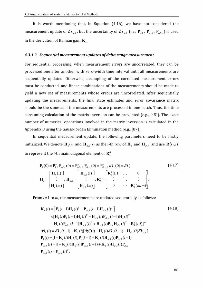
4.3 Augmentation of system state vector (1st Method)
107
It is worth mentioning that, in Equation (4.16), we have not considered the measurement update of ,ˆ d kδ x , but the uncertainty of ,ˆ d kδ x (i.e., ,d k−P , ,dc k
−P , ,cd k−P ) is used in the derivation of Kalman gain kK .
4.3.1.2 Sequential measurement updates of delta range measurement For sequential processing, when measurement errors are uncorrelated, they can be processed one after another with zero-width time interval until all measurements are sequentially updated. Otherwise, decoupling of the correlated measurement errors must be conducted, and linear combinations of the measurements should be made to yield a new set of measurements whose errors are uncorrelated. After sequentially updating the measurements, the final state estimates and error covariance matrix should be the same as if the measurements are processed in one batch. Thus, the time consuming calculation of the matrix inversion can be prevented (e.g., [45]). The exact number of numerical operations involved in the matrix inversion is calculated in the Appendix B using the Gauss-Jordan Elimination method (e.g., [87]). In sequential measurement update, the following parameters need to be firstly initialized. We denote ( )k iH and , ( )d k iH as the i-th row of kH and ,d kH , and use ( , )k i iφR to represent the i-th main diagonal element of k
φR . , , , ,
,
,
,
ˆ ˆ(0) , (0) , (0) , (0)
(1) (1) (1,1) 0
, , .
( ) ( ) 0 ( , )
k k cd k cd k dc k dc k k k
k d k k
k d k k
k d k km m m m
φ
φ
φ
δ δ− − − −= = = =
= = =
P P P P P P x x
H H R
H H R
H H R
(4.17)
From i =1 to m, the measurements are updated sequentially as follows: , ,
, ,
1, , , , ,
( ) ( 1) ( ) ( 1) ( )
[ ( ) ( 1) ( ) ( ) ( 1) ( )
( ) ( 1) ( ) ( ) ( ) ( , )]
ˆ ˆ( ) ( 1) ( )[ ( ) ( )
T Tk k k cd k d k
T Tk k k d k dc k k
T Tk cd k d k d k d k d k k
k k k k k
i i i i i
i i i i i i
i i i i i i i
i i i i i
φ
φδ δ δ
−
= − − − × − − −
− − + +
= − + −
K P H P H
H P H H P H
H P H H P H R
x x K y H , ,
, ,
, , , ,
, ,
ˆ ˆ( 1) ( ) ]
( ) [1 ( ) ( )] ( 1) ( ) ( ) ( 1)
( ) [1 ( ) ( )] ( 1) ( ) ( )
( ) ( ) .
k d k d k
k k k k k d k dc k
cd k k k cd k k d k d k
Tdc k cd k
i i
i i i i i i i
i i i i i i
i i
δ δ− += − − + −
= − − +
=
x H x
P K H P K H P
P K H P K H P
P P
(4.18)

4.3 Augmentation of system state vector (1st Method)
108
4.3.1.3 Measurement update of pseudorange measurements The batch processing of pseudorange measurements is conducted after we process the delta range measurements. The a posteriori estimates from delta range measurement update (i.e., ˆ kδ +x and k+P in Equation (4.18)) are used here as a priori estimates (i.e., ˆ kδ −x and k
−P ) in Equation (4.19). 1( )
ˆ ˆ ˆ[ ]
( ) .
T Tk k k k k k k
k k k k k k
k k k k
ρ
ρδ δ δ δ
− − −
+ − −
+ −
= +
= + −
= −
K P H H P H R
x x K y H x
P I K H P (4.19)
For sequential processing, we define: (1) (1,1) 0
, .
( ) 0 ( , )
k k
k k
k km m m
ρ
ρ
ρ
= =
H R
H R
H R
(4.20) From i =1 to m, the measurements are sequentially updated as:
1( ) ( 1) ( ) [ ( ) ( 1) ( ) ( , )]
ˆ ˆ ˆ( ) ( 1) ( )[ ( ) ( ) ( 1)]
( ) [1 ( ) ( )] ( 1).
T Tk k k k k k k
k k k k k k
k k k k
m i m i i i m i i i i
m i m i m i i i m i
m i m i i m i
ρ
ρδ δ δ δ
−+ = + − + − +
+ = + − + + − + −+ = − + + −
K P H H P H R
x x K y H x
P K H P (4.21) After all measurements are updated, the a posteriori estimates are calculated as:
ˆ ˆ ( ), ( ).k k k km m m mδ δ+ += + = +x x P P (4.22) They are used as the delay states and covariance parameters in the next recursion:
, 1 , 1ˆ ˆ ( ), ( ).d k k d k km m m mδ δ+ += + = +x x P P (4.23) The whole process repeats at the next epoch. 4.3.2 Computational burden analysis
It is known that the sequential processing can save computational time. But how much can be exactly saved? In order to answer this question, the number of numerical operations involved in the additions and multiplications should be counted separately. The method utilized in [48] has been employed in this chapter, where subtraction is

4.3 Augmentation of system state vector (1st Method)
109
counted as addition and the division over scalar is considered as multiplication by the inverse of the scalar. The “n” represents the dimension of state vector and “m” is the dimension of the observation vector. We denote the “nn” as an n-by-n square matrix, and “nn×nn” stands for an n-by-n matrix multiplies another n-by-n matrix. “n1” means an n-dimensional vector, “1” means a scalar value. The numbers in the column of “Num.” represent the amount of operations involved in the measurement update of both pseudorange and delta range measurements, while the numbers in the parentheses denote the operations encountered in the delta range measurement update only. For measurement update in one batch (i.e., Equation (4.16) and (4.19)), the involved numerical operations are given in the left side of Table 4-1. For measurement update in sequence (i.e., Equation (4.18) and (4.21)), they are given in the right side of Table 4-1 summaries the overall conducted numerical operations involved in sequential and batch measurement updates. Table 4-1. Numerical operations involved in sequential and batch measurement updates. Batch processing Sequential processing Operation Num. Add. Multi. Operation Num. Add. Multi.nn nm× 3(2) ( 1)n nm− 2mn 1nn n× 3(2)× m ( 1)n n − 2n nm mn× 5(4) 2( 1)m n− 2mn 1 1n n+ 3(2)×m n − nm nm+ 1(1) nm − 1n nn× 10(8)× m ( 1)n n − 2n nm mm× 2(1) ( 1)m mn− 2nm 1 1n n× 8(6)×m 1n − n mn nn× 10(8) ( 1)mn n − 2mn 1 1+ 8(6)× m 1 − mn nm× 5(4) 2( 1)n m− 2nm 1 1× 2(1)×m − 1 mm mm+ 5(4) 2m − 1 1n × 4(2)× m − n nn nn+ 5(4) 2n − 1 1n n× 5(4)×m − 2n
1mn n× 3(2) ( 1)m n − mn nn nn+ 5(4)× m 2n − 1 1m m+ 3(2) m −
1nm m× 2(1) ( 1)m n− nm 1 1n n+ 2(1) n −
inv( )mm 2(1) 3 232
2 2
mm m− + 33 1
2 2m m−
Table 4-2. Computational burden comparison. Operations Additions Operations Multiplications Batch 3 2 23 (7 4) (18 9 1)m n m n n m+ − + − + Batch 3 2 23 7 (18 5 1)m nm n n m+ + + − Sequential 2(18 2 )n n m− Sequential 2(18 12 2)n n m+ +

4.3 Augmentation of system state vector (1st Method)
110
The correctness of calculations in Table 4-2 can be easily verified when we consider the case that there is only one satellite in view (m=1). In this case, there should be no difference between the sequential and batch processing. We can prove this by assigning m to be 1. The batch processing returns 218 2n n− for additions, and 218 12 2n n+ + for multiplications, which equals to the required operations from sequential processing. Based on the results shown in Table 4-2, the relationships between the number of numerical operations and the dimension of the observation vector are illustrated in
Figure 4-1 and Figure 4-2, where the dimension of the state vector is 17 (i.e., n=17). Figure 4-1 shows that if more measurements are processed, more computational time can be saved by sequential processing. However, if the number of measurements is smaller than 4, no big difference can be observed. In this chapter, we update the delta range and pseudorange as two batches of data. And hence, the dimension of observation vector is always smaller than 11 (i.e., m ≤ 11), which saves a large amount of numerical operations. Figure 4-2 illustrates that the measurement update of the delta range requires much more numerical operations than those from the pseudorange measurement update (i.e., increased computational complexity in Equation (4.18) as compared with Equation (4.21)). However, when compared with batch processing (i.e., red curves in Figure 4-2), the advantage of applying sequential measurement update is obvious.

4.3 Augmentation of system state vector (1st Method)
111
Figure 4-1. Computational burden analysis (addition versus multiplication).
Figure 4-2. Computational burden analysis (pseudorange versus delta range).

4.4 Backward prediction of delay states by current states (2nd method)
112
4.4 Backward prediction of delay states by current states (2nd
method)
In the second method, we predict the delay states backwards by current states considering the integrated system process noises. Equation (4.6) is repeated here for convenience 1 1 .k k k k k k
φ φδ δ δ− −= − +y H x H x v After the backward prediction, the delay states are represented by current states as: , 1 1 1 1 1, 1, 1.k k k k k k k k k k k kδ δ δ δ− − − − − − −= + → = −x Φ x w x Φ x Φ w (4.24)
Substituting 1kδ −x from Equation (4.24) into Equation (4.6) yields: 1 1, 1, 1
1 1, 1 1, 1
( )
( ) ( ) .
k k k k k k k k k k k
k k k k k k k k k k
φ φ
φ
δ δ δ
δ− − − −
− − − − −
= − − +
= − + +
y H x H Φ x Φ w v
H H Φ x H Φ w v (4.25) We denote the matrices in parentheses as:
1 1, 1 1, 1and .k k k k k k k k k k− − − − −= − =M H H Φ W H Φ w (4.26) System and observation models can be re-formulated as:
, 1 1 1
with ~ (0, ), ~ (0, ).
k k k k k
k k k k k
k k k k
φ φ
φ φ
δ δ
δ δ− − −= +
= + +
x Φ x w
y M x W v
w Q v R (4.27)
In Equation (4.27), the newly formulated measurement noise ( )k kφ+W v contains the system noise 1k−w . Hence, the cross-correlation between system process noise and measurement noise must be considered. The covariance of the correlated noises is calculated as:
, 1 1
1 1 1, 1
1 1, 1
[ ( ) ]
[ ( ) ]
( ) .
Tk k k k k
Tk k k k k k
T Tk k k k
E
E
φ
φ
− −
− − − −
− − −
= +
= +
=
C w W v
w H Φ w v
Q Φ H
(4.28)

4.4 Backward prediction of delay states by current states (2nd method)
113
The measurement error covariance matrix for the new formulated system observation model (i.e., in Equation (4.27)) is computed as: , 1
1 1, 1 1 1, 1
1 1, 1 1, 1
1 1 1
[( )( ) ]
[( )( ) ]
( )
where [ ], and [ ( ) ].
cor Tk k k k k k
Tk k k k k k k k k k
T Tk k k k k k k k
T Tk k k k k k
E
E
E E
φ φ
φ φ
φ
φ φ φ
−
− − − − − −
− − − − −
− − −
= + +
= + +
= +
= =
R W v W v
H Φ w v H Φ w v
H Φ Q Φ H R
Q w w R v v
(4.29)
Thus, the KF measurement update can be summarized as 1
, 1 , 1 , 1 , 1
, 1 , 1 , 1
( )[ ]
ˆ ˆ ˆ( )
[ ] .
T T cor T Tk k k k k k k k k k k k k k k k
k k k k k k
T cor T T Tk k k k k k k k k k k k k k k
φδ δ δ δ
− − −− − − −
+ − −
+ − −− − −
= + + + +
= + −
= − + + +
Κ P M C M P M R M C C M
x x K y M x
P P K Μ P M R M C C M K
(4.30) The detail derivation of Equation (4.30) can be also found in the reference (e.g., [44]), which is omitted here. 4.4.1 Decoupling of correlated measurement errors
In Equation (4.30), the measurement error covariance matrix , 1cork k−R is full. Thus, in order to apply sequential measurement update, decoupling has to be conducted [87, 88]. For symmetric positive definite matrix , 1
cork k−R , the Jordan form decomposition is always possible (e.g., [22]), as shown in Equation (4.31).
, 1
1 1, 1 1, 1
[( )( ) ]
( )
cor Tk k k k k k
T T Tk k k k k k k k
E φ φ
φ
−
− − − − −
= + +
= + =
R W v W v
H Φ Q Φ H R UDU (4.31)where U is an orthonormal matrix (i.e., T =U U I ), which contains the eigenvectors of
, 1cork k−R , and D is the diagonal matrix containing the eigenvalues of , 1
cork k−R . The equivalent measurement vector s
kδ y , diagonal matrix , 1sk k−R and the transformed observation matrix s
kM are computed as: , 1
1 1, 1 1,
[ ( )( ) ]=
.
s Tk k
s T T T Tk k k k k k
s T T T s sk k k k k k k k k k
E
φ
φ φ
δ δ
−
− − − −
=
= + + =
= = − = −
y U y
R U W v W v U U UDU U D
M U M U H U H Φ H H Φ (4.32)

4.4 Backward prediction of delay states by current states (2nd method)
114
4.4.2 Computational burden analysis
After the decoupling of correlated measurement errors, sequential processing can be applied. The newly formulated observation model and error covariance matrix are used, and the following parameters are initialized. , 1 1 1, 1
, 1
, 1
, 1
ˆ ˆ(0) , (0) , ( ) ( ) ( )
(1) (1,1) 0
,
( ) 0 ( , )
T s Tk k k k k k k k k k
s sk k k
s sk k k
s sk k k
i i
m m m
δ δ− −− − − −
−
−
−
= = =
= =
P P x x C Q Φ H
M R
M R
M R
(4.33)
where ( )sk iM denotes the i-th row of s
kM , and , 1( , )sk k i i−R represents the i-th diagonal element of , 1
sk k−R . From i =1 to m, the delta ranges are sequentially updated as:
, 1
1, 1 , 1 , 1
( ) [ ( 1) ( ) ( )]{ ( ) ( 1) ( )
( , ) ( ) ( ) ( ) ( ) }
ˆ ˆ ˆ( ) ( 1) ( )[ ( ) ( ) ( 1)]
( ) ( 1) ( ){ ( ) ( 1) (
s T s s Tk k k k k k k k
s s T s Tk k k k k k k k
s sk k k k k
s sk k k k k k
i i i i i i i
i i i i i i
i i i i i i
i i i i i
δ δ δ δ
−
−− − −
= − + −
+ + +
= − + − −
= − − −
K P M C M P M
R M C C M
x x K y M x
P P K M P M , 1
, 1 , 1
) + ( , )
( ) ( ) ( ) ( ) } ( ) .
T sk k
s T s T Tk k k k k k k
i i i
i i i i i
−
− − + +
R
M C C M K
(4.34)
The sequential processing of pseudorange measurements is given in Equation (4.19) and (4.21). After sequentially updating all measurements, the a posteriori states and error covariance matrix are updated as: ˆ ˆ ( ), ( ).k k km m m mδ δ+ += + = +x x P P
(4.35)
Table 4-3 shows the computational burden involved in the sequential and batch measurement updates in this method. The relationship between the number of numerical operations and the dimension of observation vector is illustrated in Figure
4-3.

4.5 Comparisons of two approaches
115
Figure 4-3. Numerical operations involved in sequential and batch measurement updates. Table 4-3. Computational burden comparison. Operations Additions Operations MultiplicationsBatch 3 2 21.5 (8 2) (4 2 0.5)m n m n n m+ − + − + Batch 3 2 21.5 8 (4 2 0.5)m nm n n m+ + + −Sequential 2(4 6 )n n m+ Sequential 2(4 10 1)n n m+ + Figure 4-3 shows that the computational burden of sequential measurement update is smaller than that from batch processing, especially when the dimension of observation vector grows high.
4.5 Comparisons of two approaches
From the above analysis, the latter approach requires less computational burden. Nevertheless, its drawbacks are severe. Firstly, in the recursive algorithm, the inverse of transition matrix (i.e., ( )-1
1, , -1=k k k k−Φ Φ ) needs to be computed. Although this matrix inversion can be circumvented with appropriate algebraic substitutions in Equation

4.6 Simulation setup
116
(4.30) (e.g., [44]), the resultant equations for computing the Kalman gain and covariance update are still very complicated. Secondly, in the system state space models, the system noise and measurement noise are correlated with each other. This cross-correlation will significantly increase the complexity of the KF algorithm, which makes the filter difficult to be tuned. Thirdly, the , 1cork k−R is full and time-varying during the application. Therefore, the measurement decoupling step needs to be made at each step of the measurement update, which introduces additional computational burden. A concise comparison is made in Table 4-4.
Table 4-4. Comparison of methods. Problems: Method 1 Method 2 Augmented system state vector YES No Correlated system process and measurement noises No YES Decoupling of correlated measurements at measurement update rate No YES Inversion of transition matrix ( )-1
1, , -1=k k k k−Φ Φ No YES In Table 4-4, the advantages of the first method are quite clear. Although we augment the system state vector, we never perform the computation directly on the augmented system and observation models. Instead, we use the “sub-matrices” in the system and observation model (i.e., Equation (4.10) and (4.14)) to calculate the partitioned Kalman gain and update the state vectors with covariance matrices. In following sections, the first method is employed in the INS/GPS tightly-coupled integration. The remaining questions will be answered. 1. Can sequential processing successfully handle the measurement update of different types of measurements without degrading the system estimation accuracy? 2. If yes, are there any conditions, which must be met? 4.6 Simulation setup
A field collected UAV trajectory is used in the simulation. The position and velocity dynamic profiles are depicted in Figure 4-4 and Figure 4-5. For verifying the algorithm, the simulation is simplified. That is, the GPS receiver is assumed to be running at DGPS mode. Therefore, the majority of GPS measurement errors are corrected or minimized

4.6 Simulation setup
117
to small values, i.e., the ionospheric and tropospheric delays, satellite clock errors. And hence, they are neglected in this simulation. For the INS/GPS integration, we assume that a high level GPS receiver is used (i.e., NovAtel DL-4plus GPS receiver). The parameters shown in Table 4-5 are used to simulate the receiver-related measurement errors. For the instantaneous Doppler shift measurements, we approximate them by the first order central difference of 50 Hz carrier phase data (i.e., ( ) ( ) ( )1 1( ) / (2 )i i i
k k kd tφ φ+ −≈ − ⋅Δ ) with thermal noise and multipath errors given in Table 4-5. The multipath errors are generated using the SATNAV toolbox. The basic idea is to form the zero-elevation angle equivalent pseudorange multipath errors using a linear autoregressive model (i.e., “filter” function in MATLAB) and scale these errors by the cosine of their elevation angles before they are applied to the range measurements. Regarding the IMU, a LandMarkTM20 eXT MEMS-IMU from Gladiator Technologies Inc. is simulated. The main sensor errors are generated according to its specification as shown in Table 4-6. The IMU raw data in body frame are plotted in Figure 4-6. For the KF, the system time-update happens at the IMU measurements update rate, which is 50 Hz, while the measurement-update happens at the GPS measurement update rate, which is 5 Hz. The simulation is conducted with 8 satellites in view.
Figure 4-4. UAV trajectory. Figure 4-5. Dynamic profiles.

4.7 Numerical result
118
Table 4-5. Parameters for receiver-related measurement errors (1 sigma). Receiver thermal noise Multipath errors Pseudorange (DLL) 0.5 m 0.4 m Doppler (FLL) 0.05 m/s 0.04 m/s Carrier phase (PLL) 0.001 m 0.004 m
Figure 4-6. Simulated LandMarkTM 20 eXT MEMS-IMU raw data. Table 4-6. LandmarkTM20 eXT MEMS-based IMU performance specification. Gyroscope (Angular rates) Bias in-run stability Noise (ARW) Scale Factor Error 20 [°/h] (1σ ) 0.035[°/s/√Hz] (1σ ) ≤ 1000 [ppm] Accelerometer (Specific forces) Bias in-run stability Noise (VRW) Scale Factor Error 20 [µg] (1σ ) 40 [µg/√Hz] (1σ ) ≤ 1000 [ppm]
4.7 Numerical result
4.7.1 System performance comparison using different approaches
This test is to show the advantage of correctly handling the errors in the delta range measurements (i.e., integrated measurements). We initialize the filter to be 1 m away to the north, east and down directions respectively from their true values. The errors analyzed here represent the norm of position, velocity and attitude errors. For instance, the norm of position errors will be calculated as 2 2 2n e dx x xΔ = Δ + Δ + Δx . The comparisons are made between the conditions listed in Table 4-7, and the results are depicted in Figure 4-7 and Figure 4-8. The “augmented” method denotes the first method introduced in this chapter (i.e., Equations (4.10) and (4.14)). The standard approach represents the method we introduced in chapter one (i.e., pure linearization based approach from Equations (1.43) and (1.45)). Joseph error

4.7 Numerical result
119
covariance update formula is used in the KF to prevent the numerical instability, which will be introduced in Appendix C. Table 4-7. Conditions for comparison. Red “Augmented” method using pseudorange and delta range measurements Green “Augmented” method using delta range measurements only Blue “Standard” method using pseudorange for position and delta range for velocityBlack “Standard” method using pseudorange for position and Doppler shift for velocity For the “augmented” approach (red curves), both code derived pseudorange and carrier-phase derived delta range measurements are related with position estimation through the system observation model (i.e., Equation (4.14)). The pseudorange measurements provide the absolute positioning information, while the delta range measurements provide the relative displacement of system position from one time instant to the next. In this test, the filter is initialized from a position, which is one meter away to the north, east and down directions respectively from their true values. In such case, when the filter gives more confidence on GPS pseudorange measurements, the position estimation errors will decrease rapidly, and the filter shows noisier performance. On the other hand, when more confidence is given on the delta range measurements, the positioning estimation errors decrease more slowly. However, the system will present much improved estimation accuracy after the transient phrase of the filter. By giving correct weights on the pseudorange and delta range measurements based on parameters shown in Table 4-5 the system performance plotted in red is obtained. In Figure 4-7, the third subplot is the “zoom-in” version of the second subplot, where the red curve represents the velocity estimation error. It shows that with correctly handling the errors involved in the delta range measurement (i.e., integrated measurement), the system can correctly track the accelerations and jerks involved in the trajectory.

4.7 Numerical result
120
Figure 4-7. Comparison of position and velocity estimation results The green curves in Figure 4-7 represent the system performances obtained from an extreme case. That is, if no pseudorange measurements (absolute positioning information) are available in the filter (i.e., having only the delta range measurements), the system presents the best velocity estimation results. However, for position, incorrect position initialization errors remain through the whole trajectory, as shown in the first subplot of Figure 4-7. The blue curves in Figure 4-7 represent the estimation results using the “standard” approach. Since the dynamics encountered in the trajectory is severe, large velocity estimation errors occur which are subject to the accelerations and jerks involved in the trajectory. The same problem can also be observed in the attitude estimation results.

4.7 Numerical result
121
Figure 4-8. Comparison of attitude estimation results. In Figure 4-8, the second subplot is the “zoom-in” version of the first subplot. In this chapter, we integrate the measurements obtained from a single GPS receiver antenna with measurements from an INS without redundant attitude information (e.g., from magnetometers or a multi-antenna GPS system), therefore no direct attitude fixes are available as measurements. In such case, the attitude errors are mainly related to the velocity estimation errors through the off-diagonal parameters in their error covariance matrices. Hence, the more accurate velocity estimates, the greater the dampening will be on the attitude errors. As an alternate approach, the Doppler measurements are typically used for velocity determination (black curves in Figure 4-7 and Figure 4-8). However, they are the raw measurements from the receiver frequency lock loop (FLL), which is known to be noisier than the carrier phase derived measurements. 4.7.2 System performance comparison using sequential and batch
measurement updates
This test is to prove that the sequential measurement update of different types of measurements can present identical system performance with respect to that of batch

4.7 Numerical result
122
measurement update. Test setup remains unchanged as the aforementioned one. Figure
4-9 plots the position, velocity and attitude estimation errors from 50 Monte Carlo runs using the “augmented” system with sequential and batch measurement updates.
Figure 4-9. System performance comparison between sequential and batch measurement updates. As depicted in the figure, both approaches present statistically comparable estimation results. Nevertheless, two rules must be obeyed. Firstly, when we process a group of measurements, which involve both integrated and non-integrated measurements, we must always process the integrated measurements (delta range measurements) before the non-integrated measurements (pseudorange measurements) to guarantee that there is no measurement update before we process the integrated measurements. Secondly, the cross covariance matrices (i.e., ,cd kP and ,dc kP ) need to be carefully treated. That is, in sequential processing, among the measurement scalar updates, the

4.8 Summary
123
cross covariance matrices, i.e., ,cd kP and ,dc kP , are updated from one measurement to the other with zero-width time interval, as shown in Equation (4.18). Without fulfilling these two requirements, we will not obtain comparable estimation results from the sequential and batch measurement updates in updating different types of measurements. 4.8 Summary
The errors involved in the delta range measurement are related to the pseudorange errors at the start and end of the integration interval. The correct handling of these errors is essential in cases that the vehicle is maneuvering under high dynamics with low GPS update rate. After comparing the two approaches proposed in this chapter, the method with the “augmented” system state vector can be considered as more suitable for practical usage. And hence, it is employed in the INS/GPS tightly-coupled integration. Simulation was conducted using a field collected UAV trajectory. Numerical results have shown that the filter can correctly track the accelerations and jerks involved in the application. Moreover, sequential processing was applied for measurement update in the KF to prevent the matrix inverse computation. 50 Monte Carlo runs have been conducted, which verified that the sequential processing can update different types of measurements (i.e., integrated and non-integrated) without degrading the system estimation accuracy, in case certain rules are obeyed.

5.1 Summary
124
5. Summary and Conclusions 5.1 Summary
This thesis is on low-cost INS/GPS integrated navigation system with focuses on the improvements of system performance (i.e., robustness and accuracy) by using more advanced sensor fusion algorithms. The aim of this work is to take advantage of the recent progress made in the field of estimation theory to handle nonlinear and non-Gaussian issues more accurately, which makes the usage of low-cost sensors in the integrated navigation system feasible. Moreover, an algorithm for high dynamic applications using delta phase measurement has been proposed in this thesis. By using additional delay states in the Kalman filter to remember the estimation errors in the start point of delta phase integration interval, the system can accurately estimate the instantaneous dynamics of a vehicle. This thesis started with the introduction of basic knowledge on low-cost L1 GPS data processing, INS principles and the integrated navigation system. The merits of an INS/GPS integrated system with respect to a standalone GPS device have been shown using a field experiment. After that, the nonlinear filtering estimation methods were discussed, with a special focus on particle filtering. The discussion started from the introduction of the general recursive Bayesian filter. In order to use it practically, assumptions must be made, which leads to the unscented Kalman filter and particle filter. As one highlight of this thesis, for overcoming the problems of the particle filter (e.g., processing load), an unscented particle filter has been proposed with the concept that we can improve the importance density function in generating particles more intelligently rather than increasing the number of particles based on a poor quality importance density function. By using the a posteriori estimates from the unscented Kalman filter to specify the importance density, the outperformance of the unscented particle filter has been observed with a dramatically reduced number of particles. In order to prove this idea, a simulation test has been made assuming a nonlinear non-Gaussian problem. Besides the simulation, field experiments were also made to compare and analyze the integration performance. Quaternions have been used as the representation of attitude in this work. Two approaches in quaternion propagation over time have been investigated and compared. From the analysis, the following conclusions

5.2 Conclusions
125
can be made: quaternion-derived system is more confident on the estimation of heading related states for land-based navigation; in an integration system, using a lower level IMU can provide similar navigation performance with respect to using a higher quality IMU, if the sensor errors can be correctly estimated; the unscented particle filter works fine in field test with a dramatically reduced number of particles, and its outperformance depends on the signal environment. If it is open sky environment, the unscented particle filter shows basically the same behavior as using the unscented Kalman filter. The work presented in this thesis is not only on land-based navigation system, but also on high dynamic UAV applications. In order to have accurate velocity estimates of a high dynamic platform, the carrier delta phase measurement can be used. However, the delta phase is a type of integrated measurements with errors strongly related to the range errors at the start and end of the integration interval. Normal methods circumvent these errors with approximations, which leads to large velocity estimation errors. For solving this problem, delay states have been used here to “remember” the range errors at the start of the integration interval. Furthermore, sequential processing has been utilized in the measurement update to avoid the time consuming matrix inversion computation in the derivation of the Kalman gain. The highlight of this work is that during sequential measurement update of integrated (delta phase) and non-integrated (range) measurements, no compromise has been made on their errors. 5.2 Conclusions
The contributions of this thesis can be summarized as: 1. A new nonlinear non-Gaussian filter (unscented particle filter) has been proposed for low-cost INS/GPS integration. Both simulation test and field experiments have been used to verify its outperformance with respect to other nonlinear filters. Numerical results have shown that it works well with a dramatically reduced number of particles, and it presents advantages when system encounters non-Gaussian problem. 2. In this thesis, quaternions have been used in the INS/GPS system as the representation of attitude, which do not exhibit singularity issue. Besides, it is more confident on the estimation of heading related states with respect to the Euler angle-based approach for land-based navigation. This thesis has provided two approaches

5.2 Conclusions
126
in the propagation of quaternions over time. Both are suitable to be used in a low-cost INS/GPS integration system. 3. For high dynamic applications, delay states have been introduced in order to accurately capture the delta phase measurement errors, so that the accurate instantaneous velocity can be estimated. 4. Sequential processing has been successfully applied on updating different types of measurements (integrated and non-integrated) without compromise made on their errors.

Appendix A: Basics on Quaternions
127
Appendix A: Basics on Quaternions Quaternions are represented as a complex number with four bases (i.e., 1, i, j, k): 1 2 3 4q q i q j q k= + + +q A-1 In this thesis, we denote ⊗ as quaternion product. The quaternion products between its bases show the following properties:
1, , ,
1, , ,
1, , ,
i i i j k i k j
j j j k i j i k
k k k i j k i i
⊗ = − ⊗ = ⊗ = −⊗ = − ⊗ = ⊗ = −⊗ = − ⊗ = ⊗ = − A-2
With above properties, the product of quaternions q and a is computed as: ( ) ( )( ) ( )
1 1 2 2 3 3 4 4 1 2 2 1 3 4 4 3
1 3 2 4 3 2 4 1 1 4 2 3 3 2 4 1
1 2 3 4 1 2 3 41
2 1 4 3 2 1 4 32
3 4 1 2 3
4 3 2 1 4
q a q a q a q a q a q a q a q a i
q a q a q a q a j q a q a q a q a k
q q q q a a a aa
q q q q a a a aa
q q q q aa
q q q q a
⊗ = − − − + + + −
+ − + − + + − +
− − − − − − − − = = − −
q a
1
2
3 4 1 2 3
4 3 2 1 4
q
q
a a a q
a a a a q
− −
A-3
As shown in equation A-3, we can easily find that ⊗q a does not equal to ⊗a q . Therefore, the quaternion multiplication is not commutative. The conjugate of quaternions q is presented as: 1 2 3 4q q i q j q k= − − −q A-4 The inverse of quaternions q is computed as:
1
2 2 2 21 2 3 4q q q q
− = =+ + +
q qq
q A-5 Quaternions are often represented in vector form as:
1q =
qq A-6

Appendix A: Basics on Quaternions
128
where [ ]2 3 4, ,T
q q q=q . Quaternions are used to compute the rotational transformation from one coordinate system to the other. Based on Euler’s theorem, given two right-handed orthogonal coordinates, one coordinate system axes can be aligned onto another by successive single rotations along fixed axes. The corresponding rotation vector is defined as that one coordinate axes can be aligned with the second coordinate axes by rotating φ radian (rotation angle magnitude) about an invariant axis (rotation axis) [8]. This invariant axis is referred to as the Euler axis. Given a unit vector u along the Euler axis, the quaternion vector q that represents the same rotational transformation is formulated as:
cos(0.5 ), with , ,
sin(0.5 )
T
x y zu u u
= =
φq u
φ u A-7 Apparently, q has the normality property (i.e., 1=q ). That is, although the quaternion vector q has four parameters, it has only three degrees of freedom. Based on Equation A-7, the computation of quaternion vector given a rotation vector [ ]1 2 3, ,
Tϕ ϕ ϕ= φ is handled as follows: 2 2 21 2 3
cos(0.5 )
, ,sin(0.5 )
ϕ ϕ ϕ = + + = =
φφ
φ u q φφφ
φ A-8 Given a quaternion vector [ ]1 2 3 4, , ,
Tq q q q=q , we can also compute its corresponding rotation vector as:
2 2 21 2 3 4
1 2 3 4
cos(0.5 ) , sin(0.5 )
2 atan 2( ), , ,T
q q q q
q q q q
= = = + +
= ⋅ =
φ φ q
φ q u q q q
A-9 The rotation vector is formulated as = ⋅φ φ u . If the quaternion vector q represents the rotation from navigation frame to body frame, the rotation matrix b
nR can be formulated using the quaternion parameters as:

Appendix A: Basics on Quaternions
129
2 2 2 21 2 3 4 2 3 1 4 1 3 2 4
2 2 2 22 3 1 4 1 2 3 4 3 4 1 2
2 2 2 22 4 1 3 1 2 3 4 1 2 3 4
2( ) 2( )
2( ) 2( )
2( ) 2( )
bn
q q q q q q q q q q q q
q q q q q q q q q q q q
q q q q q q q q q q q q
+ − − − + = + − + − − − + − − +
R A-10 An advantage of using quaternions is that the b
nR formed in this way only involves quadratic terms and does not have trigonometric functions, as shown in Equation (1.37). Thus, if a rotation matrix bnR is known, we can compute quaternion parameters as:
1
1
1
0.5 1 [1,1] [2,2] [3,3]
( [3,2] [2,3]) / 4
( [1,3] [3,1]) / 4
( [2,1] [1,2]) / 4
b b bn n n
b bn nb bn nb bn n
q
q
q
+ + +
− = − −
R R R
R Rq
R R
R R
A-11
Based on Equation (1.37), the rotation matrix bnR represented in Euler angles is formulated as:
( )T
Tb nn b
C C C S S S C C S C S S
S C S S S C C S S C C S
S C S C C
γ β γ β α γ α γ β α γ αγ β γ β α γ α γ β α γ α
β β α β α
− + = = + − −
R R A-12 From an element to element comparison in matrix from Equation A-10 and A-12, we can compute Euler angle in terms of quaternion parameters:
2 23 4 1 2 2 3
2 4 1 3
2 22 3 1 4 3 4
=atan2(2(q q -q q ),1-2(q +q ))
=asin(-2(q q +q q ))
=atan2(2(q q -q q ),1-2(q +q ))
αβγ
A-13 where atan2 denotes the four quadrant inverse tangent function.

Appendix B: Transformation of Quaternion Covariance to Euler Angle Covariance
130
Appendix B: Transformation of Quaternion Covariance to Euler Angle Covariance Due to the quaternion normalization constraint, the degree of freedom of a quaternion vector is three rather than four. Thus, if we use quaternion vector elements as states for representing attitude, the dimension of the state vector is 4 1× , but the dimension of state error covariance matrix is 3 3× . In this section, the propagation of quaternion covariance to Euler angle covariance is derived. In Appendix A, Equation A-13 shows the nonlinear relationship between the quaternion vector elements and the Euler angle elements. Based on this relationship, the propagation of quaternion covariance to Euler angle covariance can be accomplished using the covariance law as:
( )3 3 3 4 4 4 3 4
Teuler quat× × × ×=P A P A B-1 where 3 3
euler×P is the covariance matrix of Euler angle vector; 4 4
quat×P is the covariance matrix of quaternion vector; 3 4×A is the Jacobian matrix containing the partial derivatives of the Euler angle elements with respect to the quaternion elements. The Jacobian matrix 3 4×A is compuated as:
1 2 3 4
3 41 2 3 4
1 2 3 4
q q q q
q q q q
q q q q
α α α α
β β β β
γ γ γ γ
×
∂ ∂ ∂ ∂ ∂ ∂ ∂ ∂ ∂ ∂ ∂ ∂= ∂ ∂ ∂ ∂ ∂ ∂ ∂ ∂ ∂ ∂ ∂ ∂
A
B-2
where ( )
( ) ( )
2 22 2 3
2 22 22 3 1 2 41 3
2 2 2 1
2 2 1 2 2
q q q
q q q q q qq
α ⋅ ⋅ ⋅ + ⋅ −=∂
∂ ⋅ + ⋅ − + ⋅ ⋅ − ⋅ ⋅
( ) ( )( ) ( )
2 21 2 3 2 1 2 3 4
2 22 22 3 1 2 32 4
2 2 2 1 4 2 2
2 2 1 2 2
q q q q q q q q
q q q qq q q
α ⋅ ⋅ ⋅ + ⋅ − − ⋅ ⋅ ⋅ ⋅ − ⋅ ⋅=
⋅ + ⋅ − + ⋅ ⋅ − ⋅ ⋅
∂∂

Appendix B: Transformation of Quaternion Covariance to Euler Angle Covariance
131
( ) ( )( ) ( )
2 24 2 3 3 1 2 3 4
2 22 22 3 1 2 3 43
2 2 2 1 4 2 2
2 2 1 2 2
q q q q q q q q
q q q q q qq
α ⋅ ⋅ ⋅ + ⋅ − + ⋅ ⋅ ⋅ ⋅ − ⋅ ⋅−
⋅ + ⋅ − + ⋅ ⋅ − ⋅ ⋅
∂ =∂
( )
( ) ( )
2 23 2 3
2 22 22 3 14 2 3 4
2 2 2 1
2 2 1 2 2
q q q
q qq q q q q
α ⋅ ⋅ ⋅ + ⋅∂ =−
⋅ + ⋅ − + ⋅ ⋅ − ⋅ ⋅−
∂
( )3
2
1 31
2 4
2
1 2 2
q
q q qq q
β ⋅−− ⋅ ⋅ + ⋅ ⋅
∂ =∂
( )
4
2
1 3 2 42
2
1 2 2
q
qq q q q
β ⋅
− ⋅ ⋅ + ⋅
∂
⋅= −
∂
( )1
2
3 23
1 4
2
1 2 2
q
q q q qq
β ⋅= −− ⋅ ⋅ + ⋅ ⋅
∂∂
( )
2
2
3 24
1 4
2
1 2 2
q
q q q qq
β ⋅= −− ⋅ ⋅ + ⋅ ⋅
∂∂
( )
( ) ( )
2 24 3 4
2 22 23 4 1 4 31 2
2 2 2 1
2 2 1 2 2
q q q
q q q q q qq
γ ⋅ ⋅ ⋅ + ⋅ −=∂
∂ ⋅ + ⋅ − + ⋅ ⋅ − ⋅ ⋅
( )( ) ( )
2 23 3 4
2 22 23 4 12 4 2 3
2 2 2 1
2 2 1 2 2
q q q
q qq q q q q
γ ⋅ ⋅ ⋅ + ⋅ −= −
⋅ + ⋅ − + ⋅ ⋅ − ⋅ ⋅
∂∂
( ) ( )
( ) ( )
2 22 3 4 3 1 4 2 3
2 22 23 4 1 4 2 33
2 2 2 1 4 2 2
2 2 1 2 2
q q q q q q q q
q q q q q qq
γ ⋅ ⋅ ⋅ + ⋅ − + ⋅ ⋅ ⋅ ⋅ − ⋅ ⋅= −
⋅ + ⋅ − + ⋅ ⋅ − ⋅ ⋅
∂∂
( ) ( )( ) ( )
2 21 3 4 4 1 4 2 3
2 22 23 4 1 4 24 3
2 2 2 1 4 2 2
2 2 1 2 2
q q q q q q q q
q q q qq q q
γ ⋅ ⋅ ⋅ + ⋅ − − ⋅ ⋅ ⋅ ⋅ − ⋅ ⋅=
⋅ + ⋅ − + ⋅ ⋅ − ⋅ ⋅
∂∂

Appendix C: Calculation of matrix inversion using Gauss-Jordan elimination method
132
Appendix C: Calculation of Matrix Inversion using Gauss-Jordan Elimination Method The Gauss-Jordan Elimination method is one of the methods, which are widely used to calculate the inverse of a square matrix (e.g., [87]). It is done by augmenting the square matrix with an identity matrix of the same dimension, and passing through the following matrix operations:
11 12 1 11 12 1
21 22 2 1 21 22 2
1 2 1 2
1 0 0 1 0 0
0 1 0 0 1 0Multiply by to have
0 0 1 0 0 1
n n
n n
n n nn n n nn
a a a b b b
a a a b b b
a a a b b b
−
− − − − − − − − − −
A
− − − − − − − − − − A 1− A
C-1
After the Gauss-Jordan elimination, the right side of the augmented matrix is the inverse of the original square matrix. In this contribution, we firstly transform the left side of the augmented matrix (original square matrix) to be a diagonal matrix and divide the augmented matrix by its diagonal elements on each row to have an identity matrix on the left side and the inverse of original matrix on the right side. The computation is shown as follows. In the first step, we use the elementary row operations to introduce zeros in the first column beginning from the second row, which involves 2n multiplications and 2n-1 additions. 11 12 1 11 12 1
(1) (1) (1) (1) (1)22 2 21 22 2
(1) (1) (1) (1) (1)2 1 2 2
0
0
n n
n n
n nn n n nn n n
a a a b b b
a a b b b
a a b b b×
C-2
After the first step, the elements in the rows below the first will change. We indicate this by denoting the elements with a superscript, which stands for the number of arithmetic operations involved.

Appendix C: Calculation of matrix inversion using Gauss-Jordan elimination method
133
In the second step, we introduce zeros in the second column except the second row, which involves 2n-1 multiplications and 2n-2 additions. In the n-th step, we introduce zeros in the n-th column except the n-th row, which involves n+1 multiplications and n additions. ( 1) ( 1) ( 1)
11 11 12 1(1) ( 1) ( 1) ( 1)22 21 22 2
( 1) ( 1) ( 1) ( 1)1 2 2
0 0
0 0
0 0
n n nn
n n nn
n n n nnn n n nn n n
a b b b
a b b b
a b b b
− − −
− − −
− − − −×
C-3
In the last step, we divide the augmented matrix by its diagonal elements on each row to have the matrix as shown in Equation C-1. The involved numerical operations are given in Table C-1. Table C-1. Computational burden of matrix inversion. Left side Right side Steps Multi. Add. Multi. Add. Rows processed 1 n n-1 n n n-1 2 n-1 n-2 n n n-1 n-1 2 1 n n n-1 n 1 0 n n n-1 Division 0 0 n 0 n Using the summation formula:
1
( 1)
2
n
i
n ni
=
+= C-4 According to Table C-1, the number of multiplications involved in Gauss-Jordan Elimination is
( ) ( )2 2 2 2 3
1
( 1) 3 11 1 1 1
2 2 2
n
i
n nn i n n n n n n n n n
=
+( − ) + − + = ( − ) + − + = − C-5 And the required number of additions is computed as
12 3 2
1
3( 1) ( 1) 2
2 2
n
i
nn i n n n n
−
=
− + − = − + C-6

Appendix C: Calculation of matrix inversion using Gauss-Jordan elimination method
134
We can verify our computation by inverting a scalar number as an extreme example for square matrix inversion (i.e., n=1). The arithmetic operations involved contain obviously only one multiplication (division), which is the same as the results computed from Equation C-5 and C-6.

Appendix D: Sequential measurement update using Joseph covariance update formula
135
Appendix D: Sequential Measurement Update using Joseph Covariance Update Formula In Equation (4.15) and (4.19), we use the simplified formula to derive the state error covariance matrices. However, such a simplified equation is known to be numerically unstable. In practice, the symmetric Joseph formula is widely used. Using the Joseph formula, for the delta range measurement, the state covariance matrix will be updated as:
, ,,
,, , , ,
, ,, ,
=
+
kk cd k k cd kk d k
d kdc k d k dc k d k
T
k k T Tk d k k k d k
d k d k
φ
+ + − −
+ + − −
− −
× − −
I O KP P P PH H
O I KP P P P
I O K KH H R K K
O I K K
D-1
By setting ,d kK to be a zero matrix, the a posteriori error covariance matrix k+P in Equation (4.16) will be replaced by:
, ,
, , , , ,
( ) ( ) ( )
( )
T Tk k k k k k k d k dc k k k
T T T T Tk k cd k d k k k d k d k d k k k k k
φ
+ − −
− −
= − − + −
+ − + +
P I K H P I K H K H P I K H
I K H P H K K H P H K K R K D-2 And accordingly, for sequential processing, from i=1 to m, it is updated as:
, ,
, ,
, , ,
( ) [1 ( ) ( )] ( 1)[1 ( ) ( )]
( ) ( ) ( 1)[1 ( ) ( )]
[1 ( ) ( )] ( 1) ( ) ( )
( ) ( ) ( ) ( ) ( ) ( , ) ( )
Tk k k k k k
Tk d k dc k k k
T Tk k cd k d k k
T T Tk d k d k d k k k k k
i i i i i i
i i i i i
i i i i i
i i i i i i i iφ
= − − −
+ − −
+ − −
+ +
P K H P K H
K H P K H
K H P H K
K H P H K K R K
D-3
For batch processing of pseudorange measurements, we have ( ) ( )T T
k k k k k k k k kρ+ −= − − +P I K H P I K H K R K D-4
In sequential processing, from i=1 to m, we replace the ( )k m i+P in Equation (4.21) by

Appendix D: Sequential measurement update using Joseph covariance update formula
136
( ) [1 ( ) ( )] ( 1)[1 ( ) ( )]
( ) ( , ) ( )
Tk k k k k k
Tk k k
m i m i i m i m i i
m i i i m iρ
+ = − + + − − +
+ + +
P K H P K H
K R K
D-5 After the above substitutions, a set of new KF recursive equations using Joseph covariance update formula are derived. The involved computational burden from the sequential and batch measurement updates is given in Table D-1. The results are plotted in Figure D-1. Table D-1. Computational burden comparison using Joseph covariance updates formula. Operations Additions Operations Multiplications Batch 3 2 23 (19 9) (36 24 1)m n m n n m+ − + − + Batch 3 2 23 19 (36 5 1)m nm n n m+ + + − Sequential 2(36 5 5)n n m− − Sequential 2(36 24 2)n n m+ +
Figure D-1. Numerical operation comparisons using Joseph covariance update formulas. The green curves are numerical operations involved in sequential and batch measurement updates using simplified covariance update formula, as given in Figure
4-1 and Figure 4-2. The other curves are derived using the symmetric Joseph covariance update formula in the algorithm. The additional computational burden

Appendix D: Sequential measurement update using Joseph covariance update formula
137
comes from the increased computational complexity in the update of the state error covariance matrices (i.e., Equation D-1 and Equation D-4) with respect to the formulas in Equations (4.15) and (4.19). Though Joseph formula introduces extra computational load, it guarantees the stability of mathematical computation.

Reference
138
Bibliography [1] E. D. Kaplan and C. J. Hegarty, Understanding GPS Principles and Applications, 2nd ed.: Artech House, 2006. [2] P. D. Groves, Principles of GNSS, Inertial and multisensor integrated navigation systems: Artech House Publishers 2008. [3] N. El-sheimy and X. Niu. (2007) The Promise of MEMS to the Navigation Community. Inside GNSS. [4] H. Carvalho, P. Del Moral, A. Monin, and G. Salut, "Optimal nonlinear filtering in GPS/INS integration," IEEE Transactions on Aerospace and Electronic Systems, vol. 33, pp. 835 - 850, 1997. [5] F. Gustafsson, F. Gunnarsson, N. Bergman, U. Forssell, J. Jansson, R. Karlsson, and P.-J. Nordlund, "Particle filters for positioning, navigation, and tracking," IEEE Transactions on Signal Processing, vol. 50, pp. 425 - 437, 2002. [6] W. R. Hamilton, Elements of Quaternions. London, England: Longmans, green and Co., 1866. [7] U. S. C. G. N. Center, "Global Positioning System Interface Control Document (ICD-GPS-200C including IRN-200c-001 to 004)," 2000. [8] M. S. Grewal, L. R. Weill, and A. P. Andrews, Global Positioning Systems, Inertial Navigation, and Integration, 2nd ed. New Jersey: Wiley-Interscience, 2007. [9] B. Hofmann-Wellenhof, K. Legat, and M. Wieser, Navigation principles of positioning and guidance. Wien: Springer-verlag, 2003. [10] B. Hofmann-Wellenhof, H. Lichtenegger, and J. Collins, Global Positioning System. Theory and Practice. Wien: Springer-Verlag, 1997. [11] P. Misra and P. Enge, Global Positioning System: Signals, Measurements, and Performance, 2nd ed.: Ganga-Jamuna Press, 2006. [12] A. B. Chatfield, Fundamentals of High Accuracy Inertial Navigation: American Institute of Aeronautics and Astronautics, 1997. [13] J. A. Farrell, Aided Navigation: GPS with High Rate Sensors. New York: Mcgraw-Hill Professional, 2008. [14] S. Hong, M. H. Lee, H.-H. Chun, S.-H. Kwon, and J. L. Speyer, "Observability of error States in GPS/INS integration," IEEE Trans. on Vehicular Technology, vol. 54, pp. 731 - 743, 2005. [15] J. T. W. Ryley, P. M. G. Silson, A. Tsourdos, and S. Jordan, "Observability of a stationary GPS aided INS," in AIAA Guidance, Navigation, and Control Conference, Toronto, Ontario, 2010. [16] I. Rhee, M. F. Abdel-Hafez, and J. L. Speyer, "Observability of an integrated GPS/INS during maneuvers," IEEE Trans. on Aerospace and Electronic Systems, vol. 40, pp. 526 - 535, 2004. [17] S. Knedlik, "Introduction to satellite navigation, inertial navigation, and GNSS/INS integration," Habilitation, University of Siegen, Siegen, 2011. [18] A. J. Haug, "A Tutorial on Bayesian Estimation and Tracking Techniques Applicable to Nonlinear and Non-Gaussian Processes," Technical report2005. [19] N. Gordon, D. Salmond, and A. F. M. Smith, "Novel Approach to Nonlinear and Non-Gaussian Baysian State Estimation," IEE Radar and Signal Processing, vol. 140, pp. 107 - 113, 1993.

Reference
139
[20] S. J. Julier, J. K. Uhlmann, and H. F. Durrant-Whyte, "A new method for the nonlinear transformation of means and covariances in filters and estimators," IEEE Trans. on Automatic Control, vol. 45, pp. 477 - 482, 2000. [21] M. S. Arulampalam, S. Maskell, G. N., and T. Clapp, "A Tutorial on Particle Filters for Online Nonlinear/Non-Gaussian Bayesian Tracking," IEEE Trans. on Signal Processing, vol. 50, pp. 174 - 188, 2002. [22] D. Simon, Optimal State Estimation: Kalman, H Infinity, and Nonlinear Approaches, 1 ed. New Jersey: John Wiley & Sons, 2006. [23] S. J. Julier and J. K. Uhlmann, "A Consistent, Debiased Method for Converting Between Polar and Cartesian Coordinate Systems," in AeroSense: Acquisition, Tracking and Pointing XI, Orlando FL, 1997, pp. 110–121. [24] S. J. Julier and J. K. Uhlmann, "Reduced sigma point filters for the propagation of means and covariances through nonlinear transformations," in American Control Conference, Anchorage AK, 2002, pp. 887 - 892. [25] S. J. Julier, "The scaled unscented transformation," in American Control Conference, Anchorage, Alaska, USA, 2002, pp. 4555 - 4559. [26] S. J. Julier and J. K. Uhlmann, "Unscented filtering and nonlinear estimation," IEEE Review, vol. 92, pp. 401 - 422, 2004. [27] R. van der Merwe and E. A. Wan, "Sigma-Point Kalman Filters for Integrated Navigation," in The 60th Annual Meeting of The Institute of Navigation, Dayton, OH, 2004, pp. 641-654. [28] R. van der Merwe, A. Doucet, N. D. Freitas, and E. Wan, "The Unscented Particle Filter," Cambridge University Engineering Department, Technical Report2000. [29] A. Doucet, S. Godsill, and C. Andrieu, "On sequential Monte Carlo sampling methods for Bayesian filtering," Statistics and Computing, vol. 10, pp. 197-208, 2000. [30] J. H. Kotecha and P. M. Djuric, "Gaussian particle filtering," IEEE Trans. on Signal Processing, vol. 51, pp. 2592 - 2601, 2003. [31] A. Doucet, J. F. G. de Freitas, and N. J. Gordon, Sequential Monte Carlo Methods in Practice (Statistics for Engineering and Information Science): Springer-Verlag, 2001. [32] A. Doucet, "On Sequential Simulation-Based Methods for Bayesian Filtering," Technical Report, Signal Processing Group, Department of Engineering, University of Cambridge, Cambridge, Technical Report1998. [33] B. Ristic, S. Arulampalam, and N. Gordon, Beyond the Kalman Filter: Particle Filters for Tracking Applications. Norwell, Massachusetts: Artech House, 2004. [34] J. MacCormick and A. Blake, "A probabilistic Exclusion Principle for Tracking Multiple Objects," in International Conference on Computer Vision, Kerkyra , Greece, 1999, pp. 572-578. [35] D. Crisan, P. D. Moral, and T. Lyons, "Non-linear Filtering Using Branching and Interacting Particle Systems," Markov Processes and Related Fields, vol. 5, pp. 293-319, 1999. [36] K. Kanazawa, D. Koller, and S. Russell, "Stochastic simulation algorithms for dynamic probabilistic networks," in The 11th annual conference on uncertainty in AI, 1995, pp. 346-351. [37] A. Smith and A. Gelfand, "Bayesian statistics without tears: A sampling-resampling perspective," American Statistician, vol. 46, pp. 84-88, 1992. [38] J. Liu and R. Chen, "Sequential Monte Carlo Methods for Dynamic Systems," Journal of the American Statistical Association, vol. 93, pp. 1032-1044, 1998.

Reference
140
[39] N. Bergman, "Recursive Bayesian Estimation: navigation and Tracking Applications," Linköping University, Linköping, Dissertation1999. [40] J. Carpenter, P. Clifford, and P. Fearnhead, "Improved particle filter for nonlinear problems," IEE Radar, Sonar & Navigation, vol. 146, pp. 2-7, 1999. [41] B. Ripley, Stochastic Simulation. New York: John Wiley & Sons, 1987. [42] G. Kitagawa, "Monte Carlo filter and smoother for non-Gaussian nonlinear state space models," Journal of Computational and Graphical Statistics, vol. 5, pp. 1-25, 1996. [43] P. Closas, C. Fernandez-Prades, J. A. Fernandez-Rubio, and D. Bernal, "Particle Filtering Strategies for Efficient Multipath Mitigation," in ION GNSS 2008, Savannah, GA, 2008, pp. 644 - 651. [44] R. G. Brown and P. Y. C. Hwang, Introduction to Random signals and Applied Kalman Filtering, 3 ed. New York: John Wiley & Sons, 1997. [45] P. S. Maybeck, Stochastic Models, Estimation and Control vol. 1. New York: Academic Press Inc., 1979. [46] D. Lerro and Y. Bar-Shalom, "Tracking with debiased consistent converted measurements versus EKF," IEEE Trans. on Aerospace and Electronic Systems, vol. 29, pp. 1015 - 1022, 1993. [47] J. L. Crassidis, "Sigma-Point Kalman Filtering for Integrated GPS and Inertial Navigation," in AIAA Guidance, Navigation, and Control Conference, San Francisco, California, 2005. [48] Y. Li, C. Rizos, J. L. Wang, P. Mumford, and W. D. Ding, "Sigma-Point Kalman Filtering for Tightly Coupled GPS/INS Integration," NAVIGATION, vol. 55, pp. 167 - 177, 2008. [49] Y. Li, J. Wang, and C. Rizos, "Comparison of the Extended and Sigma-point Kalman Filters on Inertial Sensor Bias Estimation Through Tight Integration of GPS and INS," in ION GNSS 2006, Fort Worth, TX, 2006, pp. 1625-1634. [50] Y. Li, J. Wang, C. Rizos, P. Mumford, and W. Ding, "Low-cost Tightly Coupled GPS/INS Integration Based on a Nonlinear Kalman Filtering Design," in ION NTM 2006, Monterey, CA, 2006, pp. 958-966. [51] E.-H. Shin and N. El-Sheimy, "Unscented Kalman Filter and Attitude Errors of Low-cost Inertial Navigation Systems," NAVIGATION, vol. 54, pp. 1-9, 2007. [52] E.-H. Shin, X. Niu, and N. El-Sheimy, "Performance Comparison of the Extended and the Unscented Kalman Filter for Integrated GPS and MEMS-Based Inertial Systems," in ION NTM 2005, San Diego, CA, 2005, pp. 961-969. [53] J. Wendel, J. Metzger, R. Moenikes, A. Maier, and G. F. Trommer, "A performance comparision of tightly coupled GPS/INS Navigation systems based on extended and Sigma point Kalman filter," NAVIGATION, vol. 53, pp. 21-31, 2006. [54] Y. Yi, "On improving the accuracy and reliability of GPS/INS-based direct sensor georeferencing," Ph.D Dissertation, Ohio State University, Geodetic Science and Surveying, 2007. [55] Y. Yi and D. A. Grejner-Brzezinska, "Performance Comparison of the Nonlinear Bayesian Filters Supporting GPS/INS Integration," in ION NTM 2006, Monterey, CA, 2006, pp. 977 - 983. [56] D.-J. Jwo and C.-N. Lai, "Unscented Kalman filter with nonlinear dynamic process modeling for GPS navigation," GPS Solutions, vol. 12, pp. 249-260, 2008. [57] Y. Yang, J. Zhou, and O. Loffeld, "Quaternion-based Kalman filtering on INS/GPS," in 15th International Conference on Information Fusion (FUSION 2012), Singapore, 2012.

Reference
141
[58] J. Zhou, E. Edwan, S. Knedlik, and O. Loffeld, "Low-cost INS/GPS with nonlinear filtering methods," in 13th International Conference on Information Fusion (FUSION 2010), Edinburgh, 2010. [59] J. Zhou, S. Knedlik, and O. Loffeld, "INS/GPS tightly-coupled integration using adaptive unscented particle filter," Journal of Navigation, vol. 63, pp. 491-513, 2010. [60] J. Zhou, Y. Yang, J. Zhang, and E. Edwan, "Applying Quaternion-based Unscented Particle Filter on INS/GPS with Field Experiments," in ION GNSS 2011 (Student paper award), Portland, Oregon, 2011. [61] J. Zhou, Y. Yang, J. Zhang, E. Edwan, O. Loffeld, and S. Knedlik, "Tightly-coupled INS/GPS using Quaternion-based Unscented Kalman filter," in AIAA Guidance, Navigation and Control 2011, Portland, Oregon, 2011. [62] H. L. Dyckman, S. Sloat, and B. Pettus, "Particle Filtering to Improve GPS/INS Integration," in ION GNSS 2004, Long Beach, CA, 2004, pp. 1619-1626. [63] F. Caron, M. Davy, E. Duflos, and P. Vanheeghe, "Particle Filtering for Multisensor Data Fusion With Switching Observation Models: Application to Land Vehicle Positioning," IEEE Trans. on Signal Processing, vol. 55, pp. 2703 - 2719, 2007. [64] A. Giremus, A. Doucety, A.-C. Escher, and J.-Y. Tourneret, "Nonlinear filtering approaches for INS/GPS Integration," in 12th European Signal Processing Conference, Vienna, Austria, 2004, pp. 873-876. [65] A. Giremus, J.-Y. Tourneret, and P. M. Djuric, "An improved regularized particle filter for GPS/INS integration," in 2005 IEEE 6th Workshop on Signal Processing Advances in Wireless Communications, New York, NY, 2005, pp. 1013 - 1017. [66] J. Georgy, U. Iqbal, M. Bayoumi, and A. Noureldin, "Reduced Inertial Sensor System (RISS)/GPS Integration using Particle Filtering for Land Vehicles," in ION GNSS 2008, Savannah, GA, 2008, pp. 30-37. [67] Y. Yi and D. A. Grejner-Brzezinska, "Tightly-coupled GPS/INS Integration using Unscented Kalman filter and Particle filter," in ION GNSS 2006, Fort Worth, TX, 2006, pp. 2182-2191. [68] Y. Yi and D. A. Grejner-Brzezinska, "Nonlinear Bayesian Filter: Alternative to the Extended Kalman Filter in the GPS/INS Fusion Systems," in ION GNSS 2005, Long Beach, CA, 2005, pp. 1391-1400. [69] P. Aggarwal and N. El-Sheimy, "Hybrid Extended Particle Filter (HEPF) for INS/GPS Integrated System," in ION GNSS 2009, Savannah, GA, 2009, pp. 1858 - 1866. [70] E.-H. Shin, "A Quaternion-Based Unscented Kalman Filter for the Integration of GPS and MEMS INS," in ION GNSS 2004, Long Beach, CA, 2004, pp. 1060-1068. [71] W. Khoder, B. Fassinut-Mombot, and M. Benjelloun, "Quaternion Unscented Kalman Filtering for integrated Inertial Navigation and GPS," in 11th International Conference on Information Fusion, 2008 Cologne, Germany, 2008. [72] E. J. Lefferts, F. L. Markley, and M. D. Schuster, "Kalman Filtering for Spacecraft Attitude Estimation," Journal of Guidance, Control, and Dynamics, vol. 5, pp. 417-429, 1982. [73] S. Sukkarieh, E. M. Nebot, and H. F. Durrant-Whyte, "A High Integrity IMU/GPS Navigation Loop for Autonomous Land Vehicle Applications," IEEE Trans. on Robotics and Automation, vol. 15, pp. 572-578, 1999. [74] D. H. Titterton and J. L. Weston, Strapdown Inertial Navigation Technology, 2 ed.: The institution of Electrical Engineers, 2004.

Reference
142
[75] S. Knedlik, J. Zhou, and O. Loffeld, "On position and attitude estimation for remote sensing with bistatic SAR," in Geoscience and remote sensing, P.-G. P. Ho, Ed., ed Vukovar: In-Tech, 2009, pp. 75-90. [76] J. Zhou, S. Knedlik, and O. Loffeld, "Sequential Processing of Integrated Measurements in Tightly-coupled INS/GPS Integrated Navigation System," in AIAA Guidance, Navigation, and Control Conference, Toronto, Ontario Canada, 2010. [77] J. Zhou, S. Knedlik, and O. Loffeld, "INS/GPS for High-Dynamic UAV-based Applications," International Journal of Navigation and Observation, vol. 2012, p. 11, 2012. [78] J. Zhang, E. Edwan, J. Zhou, and O. Loffeld, "Development and Investigation of Real-time Hybrid Navigation System Using a DCM Based Integration Method," in ION GNSS 2010, Portland, Oregon, 2010, pp. 2986 - 2994. [79] J. Zhang, S. Knedlik, and O. Loffeld, "Performance Investigation of Real-time MEMS-IMU/GNSS Integrated System," in ION GNSS 2009, Savannah, GA, 2009, pp. 978-986. [80] C. Hide, T. Moore, and M. Smith, "Adaptive Kalman Filtering for Low-cost INS/GPS," Journal of Navigation, vol. 56, pp. 143-152, 27 Jan 2003 2003. [81] A. H. Mohamed and K. P. Schwarz, "Adaptive Kalman Filtering for INS/GPS," Journal of Geodesy, vol. 73, pp. 193-203, 1999. [82] R. Mehra, "On the identification of variances and adaptive Kalman filtering," IEEE Transactions on Automatic Control, vol. 15, pp. 175 - 184, 1970. [83] R. Mehra, "Approaches to adaptive filtering," IEEE Trans. on Automatic Control, vol. 17, pp. 693 - 698, 1972 [84] C. Hide, T. Moore, and M. Smith, "Adaptive Kalman filtering algorithms for integrating GPS and low cost INS," in Position Location and Navigation Symposium, Monterey, USA, 2004, pp. 227 - 233. [85] D. F. Hartman, "Sequential Processing of Integrated Measurements in a Generalized Kalman Filter," in ION NTM 2002, San Diego, CA, 2002, pp. 632-638. [86] D. F. Hartman and D. B. Tyler, "New Kalman Filter Formulation for GPS Delta Pseudo Range Processing," in ION GPS 1998, Nashville, TN, 1998, pp. 1395-1400. [87] G. Strang and K. Borre, Linear Algebra, Geodesy, and GPS: Wellesley College, 1997. [88] G. J. Bierman, Factorization Methods for Discrete Sequential Estimation: Dover Publications, 2006.