A genetic algorithm for kidney transplantation matching · A genetic algorithm for kidney...
22
A genetic algorithm for kidney transplantation matching S. Goezinne Research Paper Business Analytics Supervisors: R. Bekker and K. Glorie March 2016 VU Amsterdam Faculty of Exact Sciences De Boelelaan 1081a 1081 HV Amsterdam
Transcript of A genetic algorithm for kidney transplantation matching · A genetic algorithm for kidney...
A genetic algorithm for kidney transplantation
matching
S. Goezinne
Research Paper Business Analytics
Supervisors: R. Bekker and K. Glorie
March 2016
VU Amsterdam
Faculty of Exact Sciences
De Boelelaan 1081a
1081 HV Amsterdam

Preface
Writing a research paper is a compulsory assignment in the Master Business Analytics at the VU
Amsterdam. The purpose of this paper is to answer a question on a chosen subject through research
in the field of Business Analytics.
I would like to thank K. Glorie and R. Bekker of the VU University for their time and for guiding me in
my research.

Abstract
Kidney exchange is one of the few methods that may permanently cure people with kidney failure.
Through a kidney exchange, incompatible patient-donor couples can swap donors in order to receive
a compatible kidney. There has not been a lot of research of the kidney exchange matching problem
in a dynamic situation. A genetic algorithm seems a promising direction, but it should be first
understood how a genetic algorithm can be developed for a static situation. The latter is the topic of
this paper. Three methods were tested and compared with an exact optimal solution program. All three
methods generated an optimal solution when 40 or less incompatible patient donor couples were
used. Increasing the number of couples to 100 or more resulted in none of the methods finding an
optimal solution. By tuning the third method that was created, an optimal solution was found for 100
couples. However, compared to the exact program, all of the methods had a significantly higher
runtime. An interesting future project would be to investigate if the runtime can be decreased if another
representation of the genetic algorithm is used. When generating a solution for the matching problem,
it is most important that as many couples as possible are matched. Because the genetic algorithm
does generate an optimal solution, future research can apply the genetic algorithm to a dynamic
situation and research if this algorithm saves more lives than current algorithms that are used in this
situation.

Content 1. Introduction ..................................................................................................................................... 1
1.1 Static and dynamic matching ........................................................................................................ 1
1.2 Related Work ................................................................................................................................. 2
1.3 Paper outline ................................................................................................................................. 2
2. Kidney exchange .............................................................................................................................. 3
2.1 Feasible solutions .......................................................................................................................... 4
2.2 Example with 5 nodes ................................................................................................................... 4
2.3 Example with an altruist ................................................................................................................ 5
3. Genetic algorithm ............................................................................................................................ 6
4. Model variants ................................................................................................................................. 8
4.1 Method 1: Only feasible solutions................................................................................................. 8
4.2 Method 2: Keeping infeasible solutions ........................................................................................ 9
4.3 Method 3: Mixed strategy ............................................................................................................. 9
5. Results ............................................................................................................................................... 11
6. Discussion and Future Research ........................................................................................................ 16
7. Bibliography ....................................................................................................................................... 17
8. Appendix ............................................................................................................................................ 18
Saidman generator ............................................................................................................................ 18

1
1. Introduction People that deal with end stage renal disease can potentially be cured with a kidney transplant. There
are two ways for receiving a kidney. One way is receiving a kidney from a deceased donor. However,
there are currently 481 people on the waiting list in the Netherlands waiting for a kidney transplant.
Another way is receiving a kidney from a willing living donor. Last year, there were 93 kidney
transplants with living donors. There is also a possibility that a patient finds a willing living donor, but
that patient is not compatible with the donor due to different blood type or tissue type. There can be
another couple that has the same problem. If the donor of the first couple is compatible with the patient
of the second couple and vice versa, then you can create a kidney exchange that matches
incompatible patient donor couples.
1.1 Static and dynamic matching There are two ways to match incompatible patient donor couples with each other: in a static situation
or in a dynamic one. In a static situation you create a solution with the couples that are currently
present. There are already algorithms that find an optimal solution to match these couples that
currently want to receive and donate a kidney. However, the number of couples can change in the
future. New couples can arrive and couples can leave, for example because the patient passes away
or receives a kidney from the waiting list. When this happens, the couple is not part of the exchange
anymore and the other couple that should have received a kidney has to wait until another matching
takes place. Therefore, heuristics are created that try to match as many people as possible in the
dynamic situation, where it is taken into account what might happen in the future.
There may be couples that are harder to match due to, for example, a rare blood type. In a dynamic
situation you can first match hard-to-match couples and let easy-to-match couples wait and match
them in the future with other hard-to-match couples and so help more people receive a kidney. The
waiting time in this situation is also important, because patients can’t wait too long for a kidney. The
goal would be to match as many people as possible with the shortest waiting time.
There has been some research about finding a solution in a dynamic situation where the number of
incompatible couples changes through time. Ünver (2010) derives efficient dynamic mechanisms that
maximizes the number of matched couples, but does not model a real-world population and does not
take tissue type compatibility into account. Anderson et al (2014) and Akbarpour et al (2014) both
study the dynamic model for barter exchange and market design consecutively. Akbarpour et al (2014)
discuss that their model can be extended to use couples that are less likely to have certain
characteristics than other couples, for example patients with a high level of antibodies. Anderson et al
(2014) and Akbarpour et al (2014) both discuss that there can be more research about the departure
process of couples. Although kidney exchange is an important type of barter exchange their research
is not specifically applied to kidney exchange. Dickerson et al (2012) uses potentials to guide myopic
matching in a dynamic situation. They discuss that their algorithm has a lot of parameters to learn and
that it would be interesting to develop a new learning algorithm.
As mentioned above, some improvements can be made to the current models that are created for the
kidney exchange problem in a dynamic situation. Combining these recommendations would result in a
new optimal model that uses a new learning algorithm that is specifically applied to kidney exchange
and models a real-world population. The model should also take tissue type compatibility into account,
uses couples that are less likely to have certain characteristics than other couples and should have a
new approach for modeling the departure process of couples.
A heuristic that uses a genetic algorithm might be able to create this new model, because the genetic
algorithm has not been studied yet in the dynamic situation. To research if the genetic algorithm can
be used to create this new model with the combined recommendations to the kidney exchange
problem, it first has to be studied if the genetic algorithm can be applied to a static situation.

2
This paper is about matching couples in a static situation and explore if the genetic algorithm can be
used for this kidney exchange problem, and if so, future research can also apply the genetic algorithm
to a dynamic situation.
1.2 Related Work As mentioned, there already exists algorithms that solve the kidney exchange problem in a static
situation. In the article of Abraham et al (2007) they discuss that when solving the kidney exchange
problem with a standard tree search algorithm, for example branch-and-cut in CPLEX, memory
becomes a bottleneck. When running the program with 900 or 1000 patient donor couples, CPLEX
runs out of memory. They created a new algorithm that uses an incremental problem formulation and
finds an optimal solution for 10.000 patient donor couples.
Only one article was found where the genetic algorithm was applied to the kidney exchange matching
problem in a static situation. This article of Sakthivel and Manimaran (2013) investigates the influence
of the genetic algorithm and compares this with an existing graph based optimization algorithm. This
paper shows that the genetic algorithm generates a small improvement to the number of nodes
matched and decreases the runtime. However, this paper does not explain what components were
used for the genetic algorithm and how it was applied. Therefore, the method is hard to apply to other
situations.
1.3 Paper outline This research paper is organized as follows. First the basics for a kidney exchange are explained in
chapter 2. Chapter 3 then describes the components of the genetic algorithm. Next, the genetic
algorithm is adjusted three times to optimize the solution for this kidney exchange problem. This is
described in chapter 4. The results of these three methods are presented and discussed in chapter 5.
Finally, the genetic algorithm is discussed and suggestions are made for future research in chapter 6.

3
2. Kidney exchange Before explaining how the genetic algorithm is applied, it is important to understand the details of a
kidney exchange. Figure 1 shows an example of a kidney exchange. Each number represent a
patient-donor couple that is incompatible with each other, this is also called a node. So in this example
there are three couples. If the donor of a couple is compatible with the patient of another couple, then
there exists an arc between the two couples. In this case, the donor of couple 0 is compatible with the
patient of couple 1, thus there exists an arc between these two couples. Also, the donor of couple 1 is
compatible with the patient of couple 2 and the donor of couple 2 is compatible with the patient of
couple 0. A cycle is a number of patient donor couples where the donor gives his/her kidney to the
patient of the next patient donor couple in the cycle. The last donor gives his kidney to the patient of
the first patient donor couple, so that all patients receive a kidney. A cycle can have different lengths,
starting from at least 2 couples. However, the cycle length should not be too large. The kidney
exchanges have to take place at the same time or else there is a possibility that a couple may drop out
after receiving a kidney, but before donating a kidney. Due to this rule the length of the cycle depends
on the hospital and how many transplants can be performed at the same time. In the example in figure
1, a cycle is shown with a cycle length of 3. So every patient from these 3 couples receives a kidney
and every donor donates a kidney.
Figure 1: Kidney exchange with a cycle of three couples
There are people who do not personally know a patient, but that are willing to help and offer their
kidney, these are called altruists. An example of a kidney exchange with an altruist is shown in figure
2. In this case node 0 is an altruist and thus doesn’t need to receive a kidney and so there isn’t an
arrow that goes back to node 0. Because node 2 is a patient donor couple, the donor of that couple
will give his kidney to the waiting list. This exchange with an altruist is called a chain. It always starts
with an altruist and always ends with a patient donor couple, where the donor gives his kidney to
someone from the national waiting list. A chain, like a cycle, can have different lengths starting from a
minimal length of 2. Because the chain starts with an altruist who doesn’t need a kidney in return for
donating one, the transplants does not have to occur at the same moment, however is still preferable
because of possible dropouts of the patient donor couples. Note that the maximum length of the chain
may be higher than that of the maximum cycle length. Figure 2 shows a chain with a length of 3.
Figure 2: Kidney exchange with a chain of one altruist and two couples
The goal to finding an optimal solution for a kidney exchange is to find as many cycles and chains with
as many nodes as possible.

4
2.1 Feasible solutions In this research a solution is a set of arcs that are used. A solution is feasible if cycles and chains can
be created from every arc in the solution and no arcs are left unused. Thus, the set only consists of
cycles and chains and is a solution where every arc is part of a cycle or a chain. To verify whether a
solution is feasible is not straightforward, as it depends on which arcs are used in which cycles or
chains. If an arc is used in a solution that isn’t part of a cycle or a chain, then a solution is infeasible.
An infeasible solution is not allowed as final solution, because that would consists of a patient donor
couple where the donor donates a kidney to someone, but the patient does not receive a kidney. The
goal is thus to provide an optimal feasible solution.
2.2 Example with 5 nodes To create a more graphical description of a kidney exchange an example is provided with five patient
donor couples, six arcs and no altruists. The compatibility between the couples can be seen in the
directed graph (figure 4) or in the compatibility
matrix (table 1).
Figure 4: Graph of kidney exchange with 5 nodes and 6 arcs
Based on this example the compatibility matrix is as follows, where the arc numbers are also indicated
in the graph of figure 4:
Node 0 1 2 3 4
0 0 1 0 0 0
1 0 0 1 0 0
2 0 0 0 1 0
3 0 1 0 0 1
4 0 0 0 1 0 Table 1: compatibility matrix
The number of arcs is the same as the number of times the number 1 appears in the compatibility
matrix, in this case 6 times. The following feasible cycles can be created with the following nodes n:
{n1, n2, n3} and {n3, n4}. As mentioned, the goal is to help as many people as possible receiving a
kidney, thus the optimal feasible solution consists of a cycle of nodes 1, 2 and 3, which helps three
patients. The representation of this solution consists of arcs 2, 3 and 4.
An example of an infeasible solution would be if arcs 1, 5 and 6 are used and thus nodes 1, 3 and 4
receive a kidney. This solution is infeasible because node 0 donates a kidney to node 1, but no kidney
is donated to node 0.

5
2.3 Example with an altruist The goal of the kidney exchange is to optimize the number of patients that receive a kidney. Because
altruists do not receive a kidney, they are not taken into account in the fitness function in the genetic
algorithm to find the optimal solution. Thus, altruists help to improve the solution by donating their
kidney willingly.
If node 0 is an altruist, the following chains can also be found, in addition to the earlier mentioned
cycles: {n0, n1}, {n0, n1, n2}, {n0, n1, n2, n3}, and {n0, n1, n2, n3, n4}. In this case two optimal
solutions can be found with the same fitness function of 4. The first solution uses a chain {n0, n1, n2}
and a cycle of {n3, n4}. The second solution consists of only the chain {n0, n1, n2, n3, n4}. Both
solutions use all nodes. However, because the representation consists of the used arcs, the solutions
are different. The representation of the first solution consists of arcs 1, 2, 5 and 6 and the
representation of the second solution consists of arcs 1, 2, 3 and 5.
6
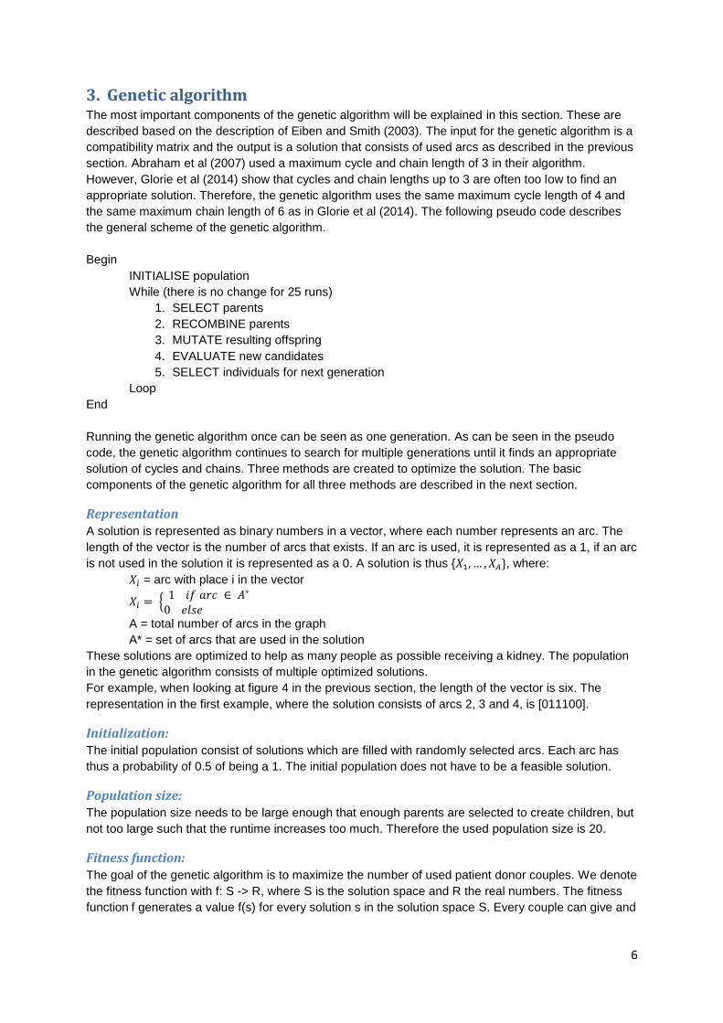
3. Genetic algorithm The most important components of the genetic algorithm will be explained in this section. These are
described based on the description of Eiben and Smith (2003). The input for the genetic algorithm is a
compatibility matrix and the output is a solution that consists of used arcs as described in the previous
section. Abraham et al (2007) used a maximum cycle and chain length of 3 in their algorithm.
However, Glorie et al (2014) show that cycles and chain lengths up to 3 are often too low to find an
appropriate solution. Therefore, the genetic algorithm uses the same maximum cycle length of 4 and
the same maximum chain length of 6 as in Glorie et al (2014). The following pseudo code describes
the general scheme of the genetic algorithm.
Begin
INITIALISE population
While (there is no change for 25 runs)
1. SELECT parents
2. RECOMBINE parents
3. MUTATE resulting offspring
4. EVALUATE new candidates
5. SELECT individuals for next generation
Loop
End
Running the genetic algorithm once can be seen as one generation. As can be seen in the pseudo
code, the genetic algorithm continues to search for multiple generations until it finds an appropriate
solution of cycles and chains. Three methods are created to optimize the solution. The basic
components of the genetic algorithm for all three methods are described in the next section.
Representation
A solution is represented as binary numbers in a vector, where each number represents an arc. The
length of the vector is the number of arcs that exists. If an arc is used, it is represented as a 1, if an arc
is not used in the solution it is represented as a 0. A solution is thus { , where:
= arc with place i in the vector
A = total number of arcs in the graph
A* = set of arcs that are used in the solution
These solutions are optimized to help as many people as possible receiving a kidney. The population
in the genetic algorithm consists of multiple optimized solutions.
For example, when looking at figure 4 in the previous section, the length of the vector is six. The
representation in the first example, where the solution consists of arcs 2, 3 and 4, is [011100].
Initialization: The initial population consist of solutions which are filled with randomly selected arcs. Each arc has
thus a probability of 0.5 of being a 1. The initial population does not have to be a feasible solution.
Population size: The population size needs to be large enough that enough parents are selected to create children, but
not too large such that the runtime increases too much. Therefore the used population size is 20.
Fitness function: The goal of the genetic algorithm is to maximize the number of used patient donor couples. We denote
the fitness function with f: S -> R, where S is the solution space and R the real numbers. The fitness
function f generates a value f(s) for every solution s in the solution space S. Every couple can give and

7
receive a kidney only once, therefore a penalty function is added to the fitness function if a node is
used more than once in a solution.
= where:
= cardinality of a set N
* = nodes that are matched
’ = nodes that are matched more than once
= penalty function for matching nodes double
The value of the penalty is higher than the number of nodes. Thus, if the number of nodes is 20, the
penalty has to be higher than 20. A solution with a positive fitness function exists of nodes that are
only matched once. A solution with a negative fitness function has matched nodes more than once
and is therefore always infeasible. The goal is finding at least one optimal feasible solution in the
population.
Parent selection: The parents are selected using ranking selection (Eiben and Smith, 2003). The solutions are sorted
based on their fitness and are then given a probability of being a parent based on their rank in the
population. The formula that Eiben and Smith use is:
Where:
= the total number of solutions
= the rank of the solution
= a number to parameterize the formula (1 < 2)
To create as many offspring as possible the probabilities are scaled, so the solution with rank -1 is
always chosen to be a parent and the solution with the lowest fitness (rank 0) will not be chosen as a
parent. To generate this we used = 2. The selected parents are then paired at random.
Recombination: The recombination method that is used is the 1-point crossover (Eiben and Smith, 2003). This method
merges the information from two randomly chosen solutions (parents) into two other solutions
(children). The 1-point crossover chooses a random place in the vector of the parents and splits both
parents at this point and creates the children by exchanging the tails.
Figure 3: 1-point crossover (Eiben and Smith, 2003)
Mutation: The mutation method that is chosen is the “each allele ” (Eiben and Smith, 2003). This method
changes the binary number in a solution with a probability of . In this algorithm the probability that a
mutation happens is = 0.1.
Survival selection:
The fitness-based replacement ( (Eiben and Smith, 2003) is used to decide which solutions
survive the current generation, where are the number of parents and are the number of
recombined and mutated children. This selection ranks all the parents and children according to their
fitness and chooses solutions with the highest fitness.
Termination: The algorithm terminates if the fitness functions does not improve for the last 25 generations.

8
4. Model variants The components of the genetic algorithm are adjusted using three different methods in order to find an
optimal solution for the kidney matching problem. All three methods use the same basic components
as described in the previous section. The components that are adjusted for each method are
described in this section.
4.1 Method 1: Only feasible solutions The first method that is created only allows feasible and optimized solutions. Therefore direct
constraint handling is used during the genetic algorithm run by restricting the search to the feasible
region. A few changes are made to the basic genetic algorithm as is described below:
Initialization
The initial population is created using a procedure that only adds feasible solutions. The procedure
starts with choosing a random node. From that node the procedure searches for a feasible cycle by
choosing random nodes. If the path that is followed doesn’t create a feasible cycle path another
random node is chosen as starting point and the procedure is repeated from the start. If the random
node that is chosen as starting point, is an altruist, then a chain is created instead of a cycle. If the
procedure finds a feasible cycle or chain, the function stops and generates the first solution with only
this cycle or chain.
For the next solutions, the same function is repeated searching for a feasible cycle or chain from the
remaining graph without the nodes used for the previous solution. Solutions are generated until the
population size is reached or until no more feasible cycles or chains can be found.
Recombination The recombination step can result in an infeasible solution. Therefore the arcs that are infeasible are
removed using the procedure that searches for feasible cycles and chains as described below. After
the infeasible arcs are removed, new arcs are added by searching for feasible cycles and chains
through the remaining unused nodes and arcs. This is done, because only optimized solutions are
allowed in this method.
Mutation The mutation step can also result in cycles and chains that are infeasible. The infeasible arcs are
again removed and new arcs are added for optimization purposes using the same procedure as
described below.
Create feasible solutions The procedure that was created to find infeasible arcs searches for cycles or chains through the
compatibility matrix, from left to right, from up to down. This procedure searches first for cycles of
length 2. With the remaining unused nodes, the procedure searches for cycles of length 3 and then
cycles of length 4 and finally searches for chains. After all the possible cycles and chains are found,
the arcs that are not used are removed from the solution.
This procedure did not perform well, because nodes that may be used for cycles of length 4 were
already used for cycles of length 2. Another procedure was created that matched more nodes.
The adjusted procedure to find infeasible arcs searches randomly for cycles of length 2, 3, 4 or chains.
With a probability of 0.25 one of the three cycle lengths or chains is chosen and the procedure
searches for cycles of only this chosen length or only searches for chains. When the procedures
searches for chains, it searches first for altruists and then tries to create a chain as long as possible.
Then with a probability of 0.33 one of the remaining three possibilities is chosen and the procedure
only searches for cycles of this length or only searches for chains. The procedure continues until the
procedure went through all four possibilities. After all the possible cycles and chains are found, the
arcs that are not used are removed from the solution.

9
Pseudocode Begin
INITIALISE population
While (there is no change for 25 runs)
1. SELECT parents
2. RECOMBINE parents
3. Make parents and children feasible
4. MUTATE resulting offspring
5. Make parents and children feasible
6. EVALUATE new candidates
7. SELECT individuals for next generation
Loop
End
4.2 Method 2: Keeping infeasible solutions The second method that is created only uses infeasible solutions. In order to find an appropriate
solution, infeasible solutions that matches nodes more than once receive a penalty. The fitness
function = thus generates a lower fitness for solutions that matches more
nodes multiple times and a higher fitness for solutions that matches less nodes more than once.
The final solution has to be feasible so that it can be used in practice. After the genetic algorithm has
found an optimal population, the solutions are made feasible and are optimized. This is done using the
same procedure as method 1.
Pseudocode Begin
INITIALISE population
While (there is no change for 25 runs)
1. SELECT parents
2. RECOMBINE parents
3. MUTATE resulting offspring
4. EVALUATE new candidates with penalty for infeasible solutions
5. SELECT individuals for next generation
Loop
Make final population feasible
End
4.3 Method 3: Mixed strategy The third method extends method 2, but after every k (a predefined number) generations, the solutions
are made feasible and are optimized using the same procedure as in method 1. For the instances in
this paper k = 20.
This method originally resulted in the same solutions that were generated with method 1. The
recombination and mutation steps often result in infeasible solutions. These infeasible solutions would
receive a fitness below 0 and would not win from the feasible solutions with a fitness above 0, because
of the penalty in the fitness function and thus would not survive. As a result there were no changes in
the population between every k generations. To make sure this doesn’t happen, an adaptation was
made to the survival selection.

10
In the survival selection step the population is ranked according to their fitness. Because of the high
penalty function for infeasible solutions, the infeasible solutions have a fitness below 0 and the
feasible solutions have a fitness equal to or above 0. The solutions are separated into two groups.
From the feasible solution group one third of the solutions of the population survive to go to the next
generation and from the infeasible group two third survive from the population. This is to make sure
that the infeasible solutions have a chance to evolve and the algorithm doesn’t converge to a local
optimum.
Pseudocode Begin
INITIALISE population
While (there is no change for 25 runs)
1. SELECT parents
2. RECOMBINE parents
3. MUTATE resulting offspring
4. Every k times: Make parents and children feasible 5. EVALUATE new candidates with penalty for infeasible solutions
6. SELECT individuals for next generation with 1/3 feasible and 2/3 infeasible
Loop
Make final population feasible
End

11
5. Results The genetic algorithm starts with using the Saidman generator to create a population of a predefined
number of patient donor couples. The Saidman generator is the most commonly used generator for
creating patients and donors characteristics that are used in kidney exchanges (Saidman et al. 2006).
For the patients the blood type, sex, PRA level and, based on the PRA level, the probability of PRA
incompatibility is generated. PRA is the percentage panel reactive antibody, this entails the amount of
antibodies that are in the patient’s blood and thus gives the probability of being cross match
incompatible with a donor. For the donors is generated the blood type, whether the donor is the
husband and whether the donor is an altruist. A patient is randomly matched to a donor and if they are
incompatible they are added to the population. The probabilities that are used are presented in the
appendix.
The genetic algorithm is first run with 20 patient donor pairs. Then the algorithm is tested for
consecutively 30, 40, 50, 75, 100 and finally 200 patient donor couples. With these couples a
compatibility matrix is generated where it is visible which couples are compatible with each other.
Because the nodes are generated with the Saidman generator, they have different properties every
time the algorithm is run. Therefore, the number of arcs is also different every run. It is likely that when
the number of nodes increases, the number of arcs also increases, because there are more matches
possible between all the nodes. Figure 5 shows the number of arcs compared with the number of used
nodes.
Figure 5: Number of arcs compared to number of nodes
This graph shows that the number of arcs increases fast, when the number of nodes increases. It is
visible that there is no linear relation, but that it looks exponential. This fast increasing relationship
between the number of nodes and the number of arcs is also visible in the other tables in this section
and will be mentioned below.
The methods that are created are compared with a program that generates the optimal solution to see
how well they perform. The program that is used is created by K. Glorie and shall further be called the
exact program.
0
2000
4000
6000
8000
10000
12000
20
30
40
50
60
70
80
90
10
0
11
0
12
0
13
0
14
0
15
0
16
0
17
0
18
0
19
0
20
0
Nu
mb
er
of
arcs
Number of nodes
Number of arcs

12
Table 2 shows the number of matched nodes for different number of arcs and nodes.
Node=20 Arcs = 91
Node=30 Arcs= 180
Node=40 Arcs= 314
Node=50 Arcs=555
Node=75 Arcs=1284
Node=100 Arcs=2313
Node=200 Arcs=11201
Method 1 6 6 9 22 35 42 -
Method 2 6 6 9 21 33 39 95
Method 3 6 6 9 22 34 40 96
Exact program
6 6 9 22 35 43 108
Table 2: Number of matched nodes
If we look at table 2 we see that when there are 20 nodes generated, there are 91 possible arcs.
When 30 nodes are generated, we see that there are almost twice as many arcs. However, this
doesn’t say anything about the number of people that can be matched in cycles or chains. As is visible
from the result of the exact program, the optimal solution is in both cases 6 matched couples.
Table 2 shows that the four methods all match the same number of couples until 40 nodes. When we
look at 50 nodes we see that method 2 using infeasible solutions, matches 1 couple less than the
optimal solution. When more nodes are used, method 2 performs slightly worse than the other two
created methods. Method 1 matches most couples compared to the other two created methods. Table
2 also shows that when the number of nodes is 100, method 1 matches only 1 couple less than the
exact program. When the program is run with 200 nodes, the runtime of method 1 exceeded 17 hours
and the program was terminated before it could provide a solution, see table 3. Method 2 and 3
perform almost the same, but the difference between their solution and the exact program is larger
than when the number of nodes is smaller. When the program is run with 500 nodes, the runtime even
exceeded 24 hours. Table 3 shows the runtime of the different situations.
Node=20 Arcs = 91
Node=30 Arcs=180
Node=40 Arcs= 314
Node=50 Arcs=555
Node=75 Arcs=1284
Node=100 Arcs=2313
Node=200 Arcs=11201
Method 1 1.41 8.00 42.05 90.81 774.35 11298.07 > 61200.00
Method 2 1.01 1.09 1.82 4.59 23.12 431.38 56726.97
Method 3 0.81 2.01 12.88 32.07 308.64 1095.98 57800.75
Exact program
0.34 0.22 0.25 0.41 0.94 1.16 2.60
Table 3: Runtime in seconds
The first thing that stands out from table 3 is that the runtime of the exact program is much lower than
any of the created methods. This is probably because the created methods have to go through a lot of
possible cycles and chains to find a solution. Especially making the solutions feasible increases the
runtime a lot. There is not much difference between the runtime of the three created methods when
the number of nodes is 20. When the number of nodes increases it is clear that method 2 has the
lowest runtime and method 1 the highest. Method 2 makes the solutions only feasible at the end of the
program and therefore has the lowest runtime. Method 1 creates feasible solutions every run and
therefore has the highest runtime.
Another notable result is that the runtime of the created methods rises fast when the number of nodes
increase. The program has to search through all the arcs to find a feasible cycles and chains.
Therefore, when the number of nodes increases, the number of arcs increases fast and also the
runtime. As we can see when looking at 200 nodes, the number of arcs is already 11201.

13
Changing the termination function Because none of the methods provided the same result as the exact program when the number of
nodes is 100 or higher, the termination function was removed to see if this had any effect. The
program then terminated after a solution was found that was the same as the optimal solution from
the exact program. This adjustment resulted in an optimal solution using method 3 and only when the
number of nodes is 75 and 100. When applying this to method 3 with 200 nodes, the runtime was very
long. This was also the case when applying this to method 1, when the number of nodes was 100 or
higher. This adjustment did not have any affect when it was applied to method 2. Method 2 only makes
the final solution feasible once and therefore running the program longer does not change the solution.
Before we used that the program terminates if the same fitness is generated for 25 times. When this
termination function was removed, method 3 found an optimal solution when the number of nodes is
75 or 100. Because changing the termination function did not provide an improved solution or resulted
in a very long runtime in the other situations, only the results of method 3 when using the number of
nodes of 75 and 100 are adjusted and presented in tables 4 and 5.
Node=20 Arcs = 91
Node=30 Arcs=180
Node=40 Arcs= 314
Node=50 Arcs=555
Node=75 Arcs=1284
Node=100 Arcs=2313
Node=200 Arcs=11201
Method 1 6 6 9 22 35 42 -
Method 2 6 6 9 21 33 39 95
Method 3 6 6 9 22 35 43 96
Exact program
6 6 9 22 35 43 108
Table 4: Number of nodes matched
Table 4 shows that method 3 now also finds the optimal solution in the case of 75 and 100 nodes.
However, as table 5 shows, removing the termination function leads to a higher runtime. When the
number of nodes is 75, the runtime is almost as long as the runtime of method 1. In the case of 100
nodes, the runtime of method 3 is more than twice the runtime of method 1, but method 1 does not
find the optimal solution and method 3 does. Due to the high runtime, the program was not run with
200 nodes.
Node=20 Arcs = 91
Node=30 Arcs=180
Node=40 Arcs= 314
Node=50 Arcs=555
Node=75 Arcs=1284
Node=100 Arcs=2313
Node=200 Arcs=11201
Method 1 1.41 8.00 42.05 90.81 774.35 11298.07 > 61200.00
Method 2 1.01 1.09 1.82 4.59 23.12 431.38 56726.97
Method 3 0.81 2.01 12.88 32.07 747.40 23852.48 57800.75
Exact program
0.34 0.22 0.25 0.41 0.94 1.16 2.60
Table 5: Runtime in seconds
Comparison of solutions When looking at the solutions that the different methods generate, we see that there is not just one
optimal solution, but that every method generates a different one. A new instance was created and
table 6 shows an example of the number of cycles and chains that are used in the solution of this new
instance. In this example, the number of nodes is 50 and the optimal solution is 26 matched couples.
Method 2 did not generate an optimal solution, but instead matched 22 couples. We see that the other
three methods all generated different solutions, but all optimal. So the optimal solution does not have
a specific number of cycles and chains and there can be multiple combinations that generate an
optimal solution.

14
Method 1 Method 2 Method 3 Exact Program
Cycle = 2 1 1 3 2
Cycle = 3 1 3 1 2
Cycle = 4 4 1 3 3
Chain = 2 0 0 0 0
Chain = 3 1 1 1 0
Chain = 4 1 0 1 0
Chain = 5 0 0 0 1
Chain = 6 0 1 0 0 Table 6: Number of cycles and chains
Table 7 shows the average of five examples and shows the percentage of times that the method
generates the same number of cycles and chains as the exact program. It is visible that method 1
only generates 19% of the times the same number of cycle or chain lengths as the exact program and
method 3 only 29%. Method 2 did again not provide an optimal solution, so it is likely that it does not
uses the same number of cycles and chains as the exact program. As was seen from table 6, the
combination of cycles and chains that are used in the optimal solution can be very different. Even
though methods 1 and 3 both found optimal solutions, they used different numbers of cycles and
chains compared to the exact program.
Method 1 Method 2 Method 3
Fraction of cycles/chains with same length as exact program
0,19 0,14 0,29
Table 7: Average fraction of same cycle / chain length in solution compared to the exact program
Table 8 shows the percentage of same nodes that were used in the solution of the method compared
to the exact program of the same five examples of table 7. Both method 1 and method 3 use 89% of
the same nodes as in the optimal solution of the exact program. Method 2 shows the lowest similarity
to the exact program, but method 2 did not find an optimal solution, so it uses less nodes and chains
and/or cycles. It is remarkable to see that even though the cycles and chains are different compared to
the exact program, the nodes that are used show a lot of similarity.
Method 1 Method 2 Method 3
Fraction of similar nodes as in exact program
0,89 0,82 0,89
Table 8: Average fraction of similar used nodes in solution compared to the exact program
Results Method 1 This method searches through all possible arcs to find a feasible and optimized solution every
generation. When looking at how the program improves its solution, the program finds an appropriate
solution after only one generation and making the solution feasible only once. Because the goal is to
find an optimal solution, the program has to go through almost all possible combinations of cycles and
chains. As can be seen from graph 1 the number of arcs increases fast when the number of nodes
increases. Therefore the runtime of this method also increases fast. This method has the longest run
time of the three methods, because it has to find feasible cycles and chains every generation. When
the number of nodes increases, the program has to go through a lot of arcs to search for a feasible
solution. This is the main reason that the runtime of this method is so much higher than the runtime of
the other methods. However, this method tries to improve a feasible solution every generation and this
leads to finding the most matched nodes of all three methods.

15
Results Method 2 In method 2, the algorithm terminates often with an infeasible solution. So there is a high probability
that there are a lot of infeasible arcs that need to be removed. The final solution depends on the
probability of which cycle length or chains are chosen to be added to the solution. This is only done
once and only searches for the available cycles and / or chains. As a result, there is a significant risk
that rather poor solutions are found. Therefore this method may not find an optimal solution and
matches the least amount of nodes of the three methods. This method was created in order to
decrease the high runtime of method 1. This method succeeded in accomplishing this. Because the
program searches only once for feasible cycles and chains, the runtime of this method is the shortest
compared to the other methods.
Results Method 3
This method uses the infeasible solutions to evolve and find a feasible solution. The best feasible
solutions are saved and together with the infeasible solutions improved to find an optimal solution.
This method combines the best features of the other two methods, evolving feasible solutions as in
method 1 and a lower runtime from method 2 by using infeasible solutions. If this method is terminated
too soon, it may not find an optimal solution. But letting this method run until an optimal solution is
found does increases the runtime a lot. When comparing the solutions to those of the exact program it
was found that the generated solutions of this method show most similarity of the three methods to the
exact program solutions.

16
6. Discussion and Future Research A genetic algorithm was applied to the kidney exchange matching problem using three different
methods. The method that used both feasible and infeasible solutions was proven to perform the best.
The runtime was lower than when using only feasible solutions and it matched more couples than
when mainly infeasible solutions were used. Comparing to the exact program the runtime was still
large. Searching for feasible solutions and making solutions feasible seems to be a bottleneck in the
application of a genetic algorithm for this type of matching problem.
A suggestion for future research to lower the runtime might be to first search for all the possible cycles
and chains and assign them a number. The search for solutions will then consists of combinations of
the possible cycles and chains. The representation of this problem is thus slightly different. In the
current situation, the genetic algorithm searches every generation for possible cycles and chains. In
the new situation this is only done once. Therefore, the runtime in the beginning of this new method
might take a while, but the runtime after this will likely be very fast and it would be interesting to see if
the total runtime decreases and if this leads to an acceptable runtime.
All existing algorithms for the matching problem search for a solution that matches as many couples
as possible. The runtime is preferably small, but it does not have an effect on the solution that will be
used. A solution that helps as many people as possible receive a kidney with a high runtime is always
chosen over a solution that helps less people with a lower runtime. It was found that the genetic
algorithm does generate an optimal solution for the matching problem in the static situation and can be
beneficial for future research. This paper shows that it is important to first understand how the genetic
algorithm performs in the static situation, before researching how the genetic algorithm performs in the
dynamic situation.
17
7. Bibliography
http://bl.ocks.org/rkirsling/5001347 (March 17, 2016)
http://www.transplantatiestichting.nl/cijfers/actuele-cijfers-organen (March 8, 2016)
Abraham, D. J., Blum, A., & Sandholm, T. (2007, June). Clearing algorithms for barter exchange markets: Enabling nationwide kidney exchanges. In Proceedings of the 8th ACM conference on Electronic commerce (pp. 295-304). ACM. Akbarpour, M., Li, S., & Oveis Gharan, S. (2014). Dynamic matching market design. Available at SSRN 2394319. Anderson, R., Ashlagi, I., Gamarnik, D., & Kanoria, Y. (2014) A dynamic model of barter exchange. Awasthi, P., & Sandholm, T. (2009, July). Online Stochastic Optimization in the Large: Application to Kidney Exchange. In IJCAI (Vol. 9, pp. 405-411).
Dickerson, J. P., Procaccia, A. D., & Sandholm, T. (2012, July). Dynamic Matching via Weighted Myopia with Application to Kidney Exchange. In AAAI.
Eiben, A. E., & Smith, J. E. (2003). Introduction to evolutionary computing. Springer Science & Business Media.
Glorie, K. M., van de Klundert, J. J., & Wagelmans, A. P. (2014). Kidney exchange with long chains: An efficient pricing algorithm for clearing barter exchanges with branch-and-price. Manufacturing & Service Operations Management, 16(4), 498-512.
Sakthivel, S & Manimaran, S. (2013). An optimized kidney transplantation based on genetic algorithm. International Journal of Advanced Research (Vol. 3, issue 4)
Ünver, M. U. (2010). Dynamic kidney exchange. The Review of Economic Studies, 77(1), 372-414.

18
8. Appendix
Saidman generator The probabilities that the Saidman generator uses are: Donor is an altruist 0.045 The gender of the patient: Female 0.409 Male 0.591 Probability that the donor is a spouse of the patient: Spousal donor 0.4897 Non-spousal donor 0.5103 Probability what kind of level the PRA of the patient is Low PRA level 0.7019 Medium PRA level 0.2 High PRA level 0.0981 Based on the PRA level, the probability that the patient is incompatible Low PRA incompatibility 0.05 Medium PRA incompatibility 0.1 High PRA incompatibility 0.9 If patient is female and donor is her husband, then the probability that they are incompatibility is Spousal PRA incompatibility 0.25 Probabilities for patient and donor: Blood type A 0.3373 Blood type B 0.1428 Blood type AB 0.0385 Blood type O 0.4814