A Gang of Bandits

Nicolo Cesa-BianchiUniversita degli Studi di Milano, Italynicolo.cesa-bianchi@unimi.it

Claudio GentileUniversity of Insubria, Italy

claudio.gentile@uninsubria.it

Giovanni ZappellaUniversita degli Studi di Milano, Italygiovanni.zappella@unimi.it

Abstract

Multi-armed bandit problems formalize the exploration-exploitation trade-offsarising in several industrially relevant applications, such as online advertisementand, more generally, recommendation systems. In many cases, however, theseapplications have a strong social component, whose integration in the bandit al-gorithm could lead to a dramatic performance increase. For instance, content maybe served to a group of users by taking advantage of an underlying network ofsocial relationships among them. In this paper, we introduce novel algorithmicapproaches to the solution of such networked bandit problems. More specifically,we design and analyze a global recommendation strategy which allocates a banditalgorithm to each network node (user) and allows it to “share” signals (contextsand payoffs) with the neghboring nodes. We then derive two more scalable vari-ants of this strategy based on different ways of clustering the graph nodes. Weexperimentally compare the algorithm and its variants to state-of-the-art methodsfor contextual bandits that do not use the relational information. Our experiments,carried out on synthetic and real-world datasets, show a consistent increase inprediction performance obtained by exploiting the network structure.

1 Introduction

The ability of a website to present personalized content recommendations is playing an increasinglycrucial role in achieving user satisfaction. Because of the appearance of new content, and due tothe ever-changing nature of content popularity, modern approaches to content recommendation arestrongly adaptive, and attempt to match as closely as possible users’ interests by learning good map-pings between available content and users. These mappings are based on “contexts”, that is sets offeatures that, typically, are extracted from both contents and users. The need to focus on contentthat raises the user interest and, simultaneously, the need of exploring new content in order to glob-ally improve the user experience creates an exploration-exploitation dilemma, which is commonlyformalized as a multi-armed bandit problem. Indeed, contextual bandits have become a referencemodel for the study of adaptive techniques in recommender systems (e.g, [5, 7, 15] ). In many cases,however, the users targeted by a recommender system form a social network. The network struc-ture provides an important additional source of information, revealing potential affinities betweenpairs of users. The exploitation of such affinities could lead to a dramatic increase in the quality ofthe recommendations. This is because the knowledge gathered about the interests of a given usermay be exploited to improve the recommendation to the user’s friends. In this work, an algorithmicapproach to networked contextual bandits is proposed which is provably able to leverage user simi-larities represented as a graph. Our approach consists in running an instance of a contextual banditalgorithm at each network node. These instances are allowed to interact during the learning process,

1

sharing contexts and user feedbacks. Under the modeling assumption that user similarities are prop-erly reflected by the network structure, interactions allow to effectively speed up the learning processthat takes place at each node. This mechanism is implemented by running instances of a linear con-textual bandit algorithm in a specific reproducing kernel Hilbert space (RKHS). The underlyingkernel, previously used for solving online multitask classification problems (e.g., [8]), is defined interms of the Laplacian matrix of the graph. The Laplacian matrix provides the information we relyupon to share user feedbacks from one node to the others, according to the network structure. Sincethe Laplacian kernel is linear, the implementation in kernel space is straightforward. Moreover, theexisting performance guarantees for the specific bandit algorithm we use can be directly lifted tothe RKHS, and expressed in terms of spectral properties of the user network. Despite its crispness,the principled approach described above has two drawbacks hindering its practical usage. First,running a network of linear contextual bandit algorithms with a Laplacian-based feedback sharingmechanism may cause significant scaling problems, even on small to medium sized social networks.Second, the social information provided by the network structure at hand need not be fully reliablein accounting for user behavior similarities. Clearly enough, the more such algorithms hinge onthe network to improve learning rates, the more they are penalized if the network information isnoisy and/or misleading. After collecting empirical evidence on the sensitivity of networked banditmethods to graph noise, we propose two simple modifications to our basic strategy, both aimed atcircumventing the above issues by clustering the graph nodes. The first approach reduces graphnoise simply by deleting edges between pairs of clusters. By doing that, we end up running a scaleddown independent instance of our original strategy on each cluster. The second approach treats eachcluster as a single node of a much smaller cluster network. In both cases, we are able to empiricallyimprove prediction performance, and simultaneously achieve dramatic savings in running times.We run experiments on two real-world datasets: one is extracted from the social bookmarking webservice Delicious, and the other one from the music streaming platform Last.fm.

2 Related work

The benefit of using social relationships in order to improve the quality of recommendations isa recognized fact in the literature of content recommender systems —see e.g., [5, 13, 18] and thesurvey [3]. Linear models for contextual bandits were introduced in [4]. Their application to person-alized content recommendation was pioneered in [15], where the LinUCB algorithm was introduced.An analysis of LinUCB was provided in the subsequent work [9]. To the best of our knowledge,this is the first work that combines contextual bandits with the social graph information. However,non-contextual stochastic bandits in social networks were studied in a recent independent work [20].Other works, such as [2, 19], consider contextual bandits assuming metric or probabilistic dependen-cies on the product space of contexts and actions. A different viewpoint, where each action revealsinformation about other actions’ payoffs, is the one studied in [7, 16], though without the contextprovided by feature vectors. A non-contextual model of bandit algorithms running on the nodes ofa graph was studied in [14]. In that work, only one node reveals its payoffs, and the statistical infor-mation acquired by this node over time is spread across the entire network following the graphicalstructure. The main result shows that the information flow rate is sufficient to control regret at eachnode of the network. More recently, a new model of distributed non-contextual bandit algorithmshas been presented in [21], where the number of communications among the nodes is limited, andall the nodes in the network have the same best action.

3 Learning model

We assume the social relationships over users are encoded as a known undirected and connectedgraph G = (V,E), where V = {1, . . . , n} represents a set of n users, and the edges in E representthe social links over pairs of users. Recall that a graph G can be equivalently defined in termsof its Laplacian matrix L =

[Li,j

]ni,j=1

, where Li,i is the degree of node i (i.e., the number ofincoming/outgoing edges) and, for i 6= j, Li,j equals −1 if (i, j) ∈ E, and 0 otherwise. Learningproceeds in a sequential fashion: At each time step t = 1, 2, . . . , the learner receives a user indexit ∈ V together with a set of context vectors Cit = {xt,1,xt,2, . . . ,xt,ct} ⊆ Rd. The learner thenselects some kt ∈ Cit to recommend to user it and observes some payoff at ∈ [−1, 1], a function

2

of it and xt = xt,kt . No assumptions whatsoever are made on the way index it and set Cit aregenerated, in that they can arbitrarily depend on past choices made by the algorithm.1

A standard modeling assumption for bandit problems with contextual information (one that is alsoadopted here) is to assume that rewards are generated by noisy versions of unknown linear func-tions of the context vectors. That is, we assume each node i ∈ V hosts an unknown parame-ter vector ui ∈ Rd, and that the reward value ai(x) associated with node i and context vectorx ∈ Rd is given by the random variable ai(x) = u>i x + εi(x), where εi(x) is a conditionallyzero-mean and bounded variance noise term. Specifically, denoting by Et[ · ] the conditional expec-tation E

[·∣∣ (i1, Ci1 , a1), . . . , (it−1, Cit−1 , at−1)

], we take the general approach of [1], and assume

that for any fixed i ∈ V and x ∈ Rd, the variable εi(x) is conditionally sub-Gaussian with vari-ance parameter σ2 > 0, namely, Et

[exp(γ εi(x))

]≤ exp

(σ2 γ2/2

)for all γ ∈ R and all x, i.

This implies Et[εi(x)] = 0 and Vt[εi(x)

]≤ σ2, where Vt[·] is a shorthand for the conditional

variance V[·∣∣ (i1, Ci1 , a1), . . . , (it−1, Cit−1 , at−1)

]. So we clearly have Et[ai(x)] = u>i x and

Vt[ai(x)

]≤ σ2. Therefore, u>i x is the expected reward observed at node i for context vector x.

In the special case when the noise εi(x) is a bounded random variable taking values in the range[−1, 1], this implies Vt[ai(x)] ≤ 4.

The regret rt of the learner at time t is the amount by which the average reward of the best choice inhindsight at node it exceeds the average reward of the algorithm’s choice, i.e.,

rt =

(maxx∈Cit

u>itx

)− u>it xt .

The goal of the algorithm is to bound with high probability (over the noise variables εit ) the cumu-lative regret

∑Tt=1 rt for the given sequence of nodes i1, . . . , iT and observed context vector sets

Ci1 , . . . , CiT . We model the similarity among users in V by making the assumption that nearbyusers hold similar underlying vectors ui, so that reward signals received at a given node it at timet are also, to some extent, informative to learn the behavior of other users j connected to it withinG. We make this more precise by taking the perspective of known multitask learning settings (e.g.,[8]), and assume that ∑

(i,j)∈E

‖ui − uj‖2 (1)

is small compared to∑i∈V ‖ui‖2, where ‖ ·‖ denotes the standard Euclidean norm of vectors. That

is, although (1) may possibly contain a quadratic number of terms, the closeness of vectors lyingon adjacent nodes in G makes this sum comparatively smaller than the actual length of such vec-tors. This will be our working assumption throughout, one that motivates the Laplacian-regularizedalgorithm presented in Section 4, and empirically tested in Section 5.

4 Algorithm and regret analysis

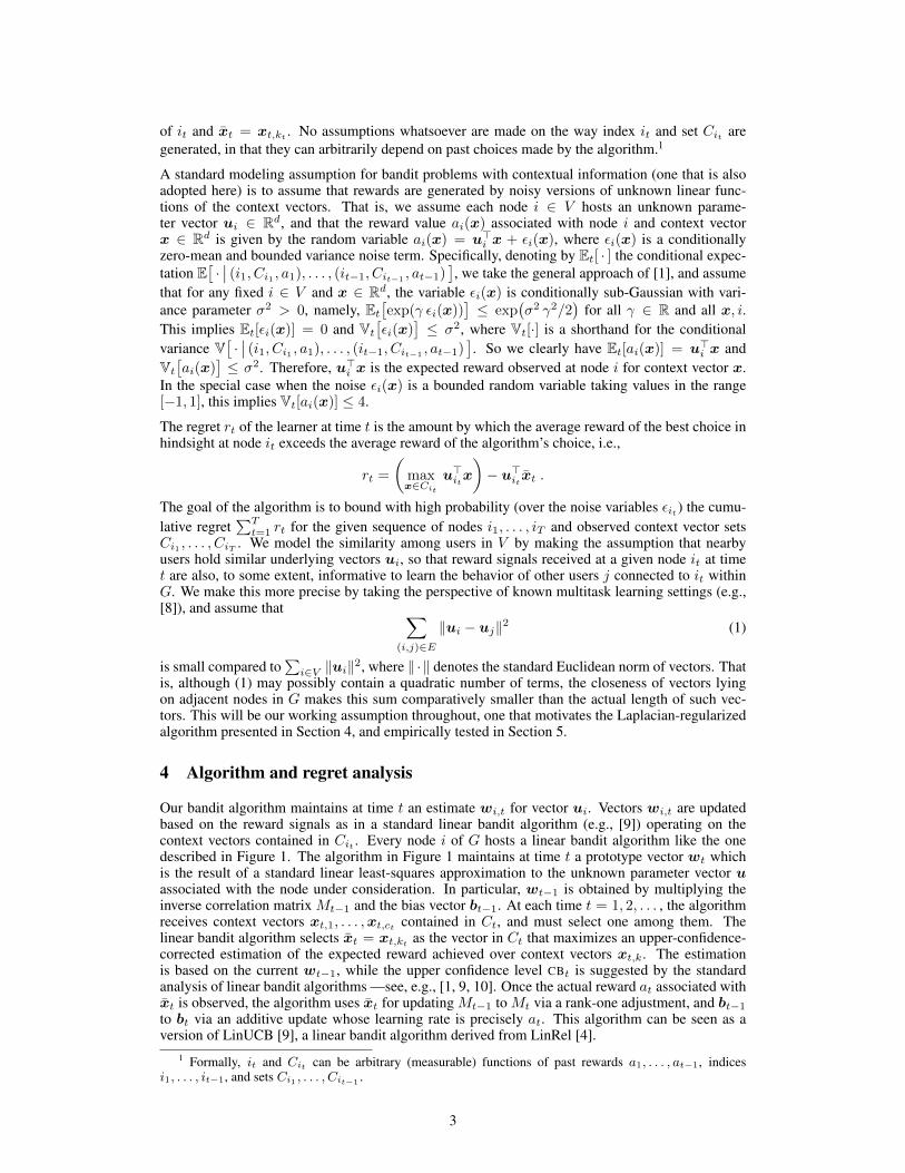
Our bandit algorithm maintains at time t an estimate wi,t for vector ui. Vectors wi,t are updatedbased on the reward signals as in a standard linear bandit algorithm (e.g., [9]) operating on thecontext vectors contained in Cit . Every node i of G hosts a linear bandit algorithm like the onedescribed in Figure 1. The algorithm in Figure 1 maintains at time t a prototype vector wt whichis the result of a standard linear least-squares approximation to the unknown parameter vector uassociated with the node under consideration. In particular, wt−1 is obtained by multiplying theinverse correlation matrix Mt−1 and the bias vector bt−1. At each time t = 1, 2, . . . , the algorithmreceives context vectors xt,1, . . . ,xt,ct contained in Ct, and must select one among them. Thelinear bandit algorithm selects xt = xt,kt as the vector in Ct that maximizes an upper-confidence-corrected estimation of the expected reward achieved over context vectors xt,k. The estimationis based on the current wt−1, while the upper confidence level CBt is suggested by the standardanalysis of linear bandit algorithms —see, e.g., [1, 9, 10]. Once the actual reward at associated withxt is observed, the algorithm uses xt for updating Mt−1 to Mt via a rank-one adjustment, and bt−1

to bt via an additive update whose learning rate is precisely at. This algorithm can be seen as aversion of LinUCB [9], a linear bandit algorithm derived from LinRel [4].

1 Formally, it and Cit can be arbitrary (measurable) functions of past rewards a1, . . . , at−1, indicesi1, . . . , it−1, and sets Ci1 , . . . , Cit−1 .

3

Init: b0 = 0 ∈ Rd andM0 = I ∈ Rd×d;for t = 1, 2, . . . , T do

Setwt−1 = M−1t−1 bt−1;

Get context Ct = {xt,1, . . . ,xt,ct};Set

kt = argmaxk=1,...,ct

(w>t−1xt,k + CBt(xt,k)

)where

CBt(xt,k) =√x>t,kM

−1t−1xt,k

σ√

ln|Mt|δ

+ ‖u‖

Set xt = xt,kt ;Observe reward at ∈ [−1, 1];Update

• Mt = Mt−1 + xtx>t ,

• bt = bt−1 + atxt .end for

Figure 1: Pseudocode of the linear bandit algo-rithm sitting at each node i of the given graph.

Init: b0 = 0 ∈ Rdn andM0 = I ∈ Rdn×dn;for t = 1, 2, . . . , T do

Setwt−1 = M−1t−1 bt−1;

Get it ∈ V , context Cit = {xt,1, . . . ,xt,ct};Construct vectors φit

(xt,1), . . . ,φit(xt,ct ), and modi-

fied vectors φt,1, . . . , φt,ct, where

φt,k = A−1/2⊗ φit

(xt,k), k = 1, . . . , ct;

Set kt = argmaxk=1,...,ct

(w>t−1φt,k + CBt(φt,k)

)where

CBt(φt,k) =

√φ>t,kM

−1t−1φt,k

σ√

ln|Mt|δ

+ ‖U‖

Observe reward at ∈ [−1, 1] at node it;Update

• Mt = Mt−1 + φt,ktφ>t,kt

,

• bt = bt−1 + atφt,k .end for

Figure 2: Pseudocode of the GOB.Lin algo-rithm.

We now turn to describing our GOB.Lin (Gang Of Bandits, Linear version) algorithm. GOB.Lin letsthe algorithm in Figure 1 operate on each node i of G (we should then add subscript i throughout,replacing wt by wi,t, Mt by Mi,t, and so forth). The updates Mi,t−1 → Mi,t and bi,t−1 → bi,tare performed at node i through vector xt both when i = it (i.e., when node i is the one which thecontext vectors in Cit refer to) and to a lesser extent when i 6= it (i.e., when node i is not the onewhich the vectors in Cit refer to). This is because, as we said, the payoff at received for node it issomehow informative also for all other nodes i 6= it. In other words, because we are assuming theunderlying parameter vectors ui are close to each other, we should let the corresponding prototypevectors wi,t undergo similar updates, so as to also keep the wi,t close to each other over time.

With this in mind, we now describe GOB.Lin in more detail. It is convenient to introduce first someextra matrix notation. Let A = In + L, where L is the Laplacian matrix associated with G, andIn is the n × n identity matrix. Set A⊗ = A ⊗ Id, the Kronecker product2 of matrices A and Id.Moreover, the “compound” descriptor for the pairing (i,x) is given by the long (and sparse) vectorφi(x) ∈ Rdn defined as

φi(x)> =(

0, . . . , 0︸ ︷︷ ︸(i−1)d times

,x>, 0, . . . , 0︸ ︷︷ ︸(n−i)d times

).

With the above notation handy, a compact description of GOB.Lin is presented in Figure 2, wherewe deliberately tried to mimic the pseudocode of Figure 1. Notice that in Figure 2 we overloadedthe notation for the confidence bound CBt, which is now defined in terms of the Laplacian L of G.In particular, ‖u‖ in Figure 1 is replaced in Figure 2 by ‖U‖, where U = A

1/2⊗ U and we define

U = (u>1 ,u>2 , . . . ,u

>n )> ∈ Rdn. Clearly enough, the potentially unknown quantities ‖u‖ and ‖U‖

in the two expressions for CBt can be replaced by suitable upper bounds.

We now explain how the modified long vectors φt,k = A−1/2⊗ φit(xt,k) act in the update of matrix

Mt and vector bt. First, observe that if A⊗ were the identity matrix then, according to how thelong vectors φit(xt,k) are defined, Mt would be a block-diagonal matrix Mt = diag(D1, . . . , Dn),whose i-th block Di is the d × d matrix Di = Id +

∑t : kt=i

xtx>t . Similarly, bt would be the

dn-long vector whose i-th d-dimensional block contains∑t : kt=i

atxt. This would be equivalentto running n independent linear bandit algorithms (Figure 1), one per node of G. Now, becauseA⊗ is not the identity, but contains graph G represented through its Laplacian matrix, the selectedvector xt,kt ∈ Cit for node it gets spread via A−1/2

⊗ from the it-th block over all other blocks,thereby making the contextual information contained in xt,kt available to update the internal status

2 The Kronecker product between two matrices M ∈ Rm×n and N ∈ Rq×r is the block matrix M ⊗N ofdimension mq × nr whose block on row i and column j is the q × r matrix Mi,jN .

4

of all other nodes. Yet, the only reward signal observed at time t is the one available at node it. Atheoretical analysis of GOB.Lin relying on the learning model of Section 3 is sketched in Section 4.1.

GOB.Lin’s running time is mainly affected by the inversion of the dn×dn matrix Mt, which can beperformed in time of order (dn)2 per round by using well-known formulas for incremental matrixinversions. The same quadratic dependence holds for memory requirements. In our experiments, weobserved that projecting the contexts on the principal components improved performance. Hence,the quadratic dependence on the context vector dimension d is not really hurting us in practice. Onthe other hand, the quadratic dependence on the number of nodes n may be a significant limitationto GOB.Lin’s practical deployment. In the next section, we show that simple graph compressionschemes (like node clustering) can conveniently be applied to both reduce edge noise and bring thealgorithm to reasonable scaling behaviors.

4.1 Regret Analysis

We now provide a regret analysis for GOB.Lin that relies on the high probability analysis containedin [1] (Theorem 2 therein). The analysis can be seen as a combination of the multitask kernelcontained in, e.g., [8, 17, 12] and a version of the linear bandit algorithm described and analyzedin [1].Theorem 1. Let the GOB.Lin algorithm of Figure 2 be run on graph G = (V,E), V = {1, . . . , n},hosting at each node i ∈ V vector ui ∈ Rd. Define

L(u1, . . . ,un) =∑i∈V‖ui‖2 +

∑(i,j)∈E

‖ui − uj‖2 .

Let also the sequence of context vectors xt,k be such that ‖xt,k‖ ≤ B, for all k = 1, . . . , ct, andt = 1, . . . , T . Then the cumulative regret satisfies

T∑t=1

rt ≤ 2

√T

(2σ2 ln

|MT |δ

+ 2L(u1, . . . ,un)

)(1 +B2) ln |MT |

with probability at least 1− δ.

Compared to running n independent bandit algorithms (which corresponds to A⊗ being the identitymatrix), the bound in the above theorem has an extra term

∑(i,j)∈E ‖ui − uj‖2, which we assume

small according to our working assumption. However, the bound has also a significantly smallerlog determinant ln |MT | on the resulting matrix MT , due to the construction of φt,k via A−1/2

⊗ . Inparticular, when the graph is very dense, the log determinant in GOB.Lin is a factor n smaller thanthe corresponding term for the n independent bandit case (see, e.g.,[8], Section 4.2 therein). To makethings clear, consider two extreme situations. When G has no edges then TR(MT ) = TR(I) + T =nd+T , hence ln |MT | ≤ dn ln(1+T/(dn)). On the other hand, WhenG is the complete graph thenTR(MT ) = TR(I) + 2t/(n+ 1) = nd+ 2T/(n+ 1), hence ln |MT | ≤ dn ln(1 + 2T/(dn(n+ 1))).The exact behavior of ln |Mt| (one that would ensure a significant advantage in practice) dependson the actual interplay between the data and the graph, so that the above linear dependence on dn isreally a coarse upper bound.

5 Experiments

In this section, we present an empirical comparison of GOB.Lin (and its variants) to linear ban-dit algorithms which do not exploit the relational information provided by the graph. We runour experiments by approximating the CBt function in Figure 1 with the simplified expression

α√x>t,kM

−1t−1xt,k log(t+ 1), and the CBt function in Figure 2 with the corresponding expression

in which xt,k is replaced by φt,k. In both cases, the factor α is used as tunable parameter. Ourpreliminary experiments show that this approximation does not affect the predictive performancesof the algorithms, while it speeds up computation significantly. We tested our algorithm and itscompetitors on a synthetic dataset and two freely available real-world datasets extracted from thesocial bookmarking web service Delicious and from the music streaming service Last.fm. Thesedatasets are structured as follows.

5

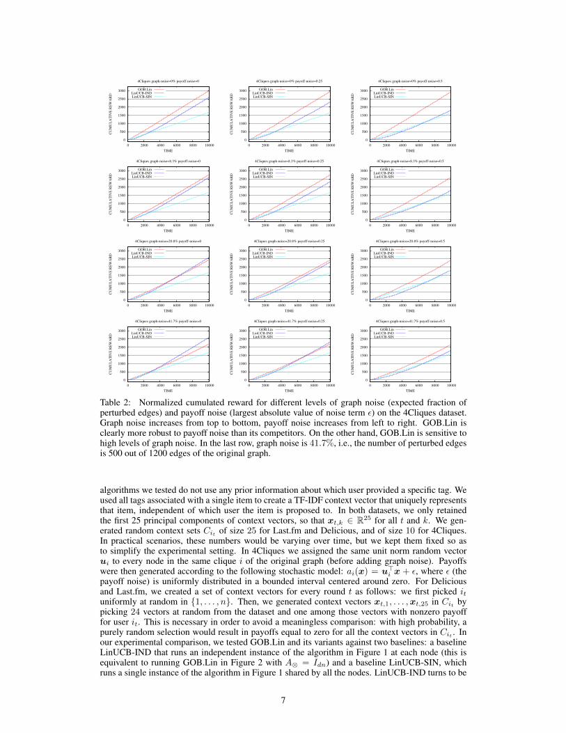
4Cliques. This is an artificial dataset whose graph contains four cliques of 25 nodes each to whichwe added graph noise. This noise consists in picking a random pair of nodes and deleting or creatingan edge between them. More precisely, we created a n×n symmetric noise matrix of random num-bers in [0, 1], and we selected a threshold value such that the expected number of matrix elementsabove this value is exactly some chosen noise rate parameter. Then we set to 1 all the entries whosecontent is above the threshold, and to zero the remaining ones. Finally, we XORed the noise matrixwith the graph adjacency matrix, thus obtaining a noisy version of the original graph.

Last.fm. This is a social network containing 1,892 nodes and 12,717 edges. There are 17,632 items(artists), described by 11,946 tags. The dataset contains information about the listened artists, andwe used this information in order to create the payoffs: if a user listened to an artist at least once thepayoff is 1, otherwise the payoff is 0.

Delicious. This is a network with 1,861 nodes and 7,668 edges. There are 69,226 items (URLs)described by 53,388 tags. The payoffs were created using the information about the bookmarkedURLs for each user: the payoff is 1 if the user bookmarked the URL, otherwise the payoff is 0.

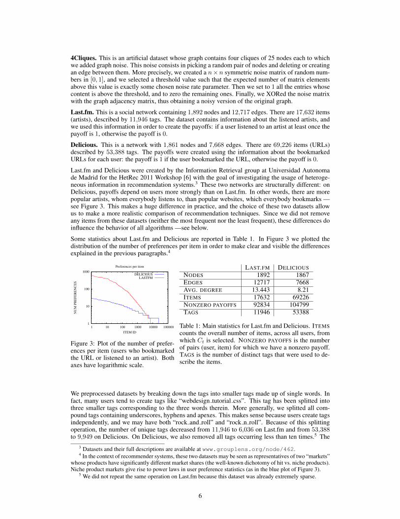
Last.fm and Delicious were created by the Information Retrieval group at Universidad Autonomade Madrid for the HetRec 2011 Workshop [6] with the goal of investigating the usage of heteroge-neous information in recommendation systems.3 These two networks are structurally different: onDelicious, payoffs depend on users more strongly than on Last.fm. In other words, there are morepopular artists, whom everybody listens to, than popular websites, which everybody bookmarks —see Figure 3. This makes a huge difference in practice, and the choice of these two datasets allowus to make a more realistic comparison of recommendation techniques. Since we did not removeany items from these datasets (neither the most frequent nor the least frequent), these differences doinfluence the behavior of all algorithms —see below.

Some statistics about Last.fm and Delicious are reported in Table 1. In Figure 3 we plotted thedistribution of the number of preferences per item in order to make clear and visible the differencesexplained in the previous paragraphs.4

1

10

100

1000

1 10 100 1000 10000 100000

NU

M P

RE

FE

RE

NC

ES

ITEM ID

Preferences per item

DELICIOUSLASTFM

Figure 3: Plot of the number of prefer-ences per item (users who bookmarkedthe URL or listened to an artist). Bothaxes have logarithmic scale.

LAST.FM DELICIOUSNODES 1892 1867EDGES 12717 7668AVG. DEGREE 13.443 8.21ITEMS 17632 69226NONZERO PAYOFFS 92834 104799TAGS 11946 53388

Table 1: Main statistics for Last.fm and Delicious. ITEMScounts the overall number of items, across all users, fromwhich Ct is selected. NONZERO PAYOFFS is the numberof pairs (user, item) for which we have a nonzero payoff.TAGS is the number of distinct tags that were used to de-scribe the items.

We preprocessed datasets by breaking down the tags into smaller tags made up of single words. Infact, many users tend to create tags like “webdesign tutorial css”. This tag has been splitted intothree smaller tags corresponding to the three words therein. More generally, we splitted all com-pound tags containing underscores, hyphens and apexes. This makes sense because users create tagsindependently, and we may have both “rock and roll” and “rock n roll”. Because of this splittingoperation, the number of unique tags decreased from 11,946 to 6,036 on Last.fm and from 53,388to 9,949 on Delicious. On Delicious, we also removed all tags occurring less than ten times.5 The

3 Datasets and their full descriptions are available at www.grouplens.org/node/462.4 In the context of recommender systems, these two datasets may be seen as representatives of two “markets”

whose products have significantly different market shares (the well-known dichotomy of hit vs. niche products).Niche product markets give rise to power laws in user preference statistics (as in the blue plot of Figure 3).

5 We did not repeat the same operation on Last.fm because this dataset was already extremely sparse.

6

0

500

1000

1500

2000

2500

3000

0 2000 4000 6000 8000 10000

CU

MU

LA

TIV

E R

EW

AR

D

TIME

4Cliques graph-noise=0% payoff-noise=0

GOB.LinLinUCB-INDLinUCB-SIN

0

500

1000

1500

2000

2500

3000

0 2000 4000 6000 8000 10000

CU

MU

LA

TIV

E R

EW

AR

D

TIME

4Cliques graph-noise=0% payoff-noise=0.25

GOB.LinLinUCB-INDLinUCB-SIN

0

500

1000

1500

2000

2500

3000

0 2000 4000 6000 8000 10000

CU

MU

LA

TIV

E R

EW

AR

D

TIME

4Cliques graph-noise=0% payoff-noise=0.5

GOB.LinLinUCB-INDLinUCB-SIN

0

500

1000

1500

2000

2500

3000

0 2000 4000 6000 8000 10000

CU

MU

LA

TIV

E R

EW

AR

D

TIME

4Cliques graph-noise=8.3% payoff-noise=0

GOB.LinLinUCB-INDLinUCB-SIN

0

500

1000

1500

2000

2500

3000

0 2000 4000 6000 8000 10000

CU

MU

LA

TIV

E R

EW

AR

DTIME

4Cliques graph-noise=8.3% payoff-noise=0.25

GOB.LinLinUCB-INDLinUCB-SIN

0

500

1000

1500

2000

2500

3000

0 2000 4000 6000 8000 10000

CU

MU

LA

TIV

E R

EW

AR

D

TIME

4Cliques graph-noise=8.3% payoff-noise=0.5

GOB.LinLinUCB-INDLinUCB-SIN

0

500

1000

1500

2000

2500

3000

0 2000 4000 6000 8000 10000

CU

MU

LA

TIV

E R

EW

AR

D

TIME

4Cliques graph-noise=20.8% payoff-noise=0

GOB.LinLinUCB-INDLinUCB-SIN

0

500

1000

1500

2000

2500

3000

0 2000 4000 6000 8000 10000

CU

MU

LA

TIV

E R

EW

AR

D

TIME

4Cliques graph-noise=20.8% payoff-noise=0.25

GOB.LinLinUCB-INDLinUCB-SIN

0

500

1000

1500

2000

2500

3000

0 2000 4000 6000 8000 10000

CU

MU

LA

TIV

E R

EW

AR

D

TIME

4Cliques graph-noise=20.8% payoff-noise=0.5

GOB.LinLinUCB-INDLinUCB-SIN

0

500

1000

1500

2000

2500

3000

0 2000 4000 6000 8000 10000

CU

MU

LA

TIV

E R

EW

AR

D

TIME

4Cliques graph-noise=41.7% payoff-noise=0

GOB.LinLinUCB-INDLinUCB-SIN

0

500

1000

1500

2000

2500

3000

0 2000 4000 6000 8000 10000

CU

MU

LA

TIV

E R

EW

AR

D

TIME

4Cliques graph-noise=41.7% payoff-noise=0.25

GOB.LinLinUCB-INDLinUCB-SIN

0

500

1000

1500

2000

2500

3000

0 2000 4000 6000 8000 10000

CU

MU

LA

TIV

E R

EW

AR

D

TIME

4Cliques graph-noise=41.7% payoff-noise=0.5

GOB.LinLinUCB-INDLinUCB-SIN

Table 2: Normalized cumulated reward for different levels of graph noise (expected fraction ofperturbed edges) and payoff noise (largest absolute value of noise term ε) on the 4Cliques dataset.Graph noise increases from top to bottom, payoff noise increases from left to right. GOB.Lin isclearly more robust to payoff noise than its competitors. On the other hand, GOB.Lin is sensitive tohigh levels of graph noise. In the last row, graph noise is 41.7%, i.e., the number of perturbed edgesis 500 out of 1200 edges of the original graph.

algorithms we tested do not use any prior information about which user provided a specific tag. Weused all tags associated with a single item to create a TF-IDF context vector that uniquely representsthat item, independent of which user the item is proposed to. In both datasets, we only retainedthe first 25 principal components of context vectors, so that xt,k ∈ R25 for all t and k. We gen-erated random context sets Cit of size 25 for Last.fm and Delicious, and of size 10 for 4Cliques.In practical scenarios, these numbers would be varying over time, but we kept them fixed so asto simplify the experimental setting. In 4Cliques we assigned the same unit norm random vectorui to every node in the same clique i of the original graph (before adding graph noise). Payoffswere then generated according to the following stochastic model: ai(x) = u>i x + ε, where ε (thepayoff noise) is uniformly distributed in a bounded interval centered around zero. For Deliciousand Last.fm, we created a set of context vectors for every round t as follows: we first picked ituniformly at random in {1, . . . , n}. Then, we generated context vectors xt,1, . . . ,xt,25 in Cit bypicking 24 vectors at random from the dataset and one among those vectors with nonzero payofffor user it. This is necessary in order to avoid a meaningless comparison: with high probability, apurely random selection would result in payoffs equal to zero for all the context vectors in Cit . Inour experimental comparison, we tested GOB.Lin and its variants against two baselines: a baselineLinUCB-IND that runs an independent instance of the algorithm in Figure 1 at each node (this isequivalent to running GOB.Lin in Figure 2 with A⊗ = Idn) and a baseline LinUCB-SIN, whichruns a single instance of the algorithm in Figure 1 shared by all the nodes. LinUCB-IND turns to be

7

0

250

500

750

1000

1250

0 2000 4000 6000 8000 10000

CU

MU

LA

TIV

E R

EW

AR

D

TIME

Last.fm

LinUCB-SIN

LinUCB-IND

GOB.Lin

GOB.Lin.MACRO

GOB.Lin.BLOCK

0

25

50

75

100

125

150

0 2000 4000 6000 8000 10000

CU

MU

LA

TIV

E R

EW

AR

D

TIME

Delicious

LinUCB-SIN

LinUCB-IND

GOB.Lin

GOB.Lin.MACRO

GOB.Lin.BLOCK

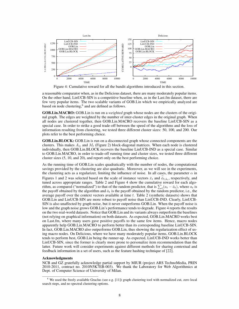
Figure 4: Cumulative reward for all the bandit algorithms introduced in this section.

a reasonable comparator when, as in the Delicious dataset, there are many moderately popular items.On the other hand, LinUCB-SIN is a competitive baseline when, as in the Last.fm dataset, there arefew very popular items. The two scalable variants of GOB.Lin which we empirically analyzed arebased on node clustering,6 and are defined as follows.

GOB.Lin.MACRO: GOB.Lin is run on a weighted graph whose nodes are the clusters of the origi-nal graph. The edges are weighted by the number of inter-cluster edges in the original graph. Whenall nodes are clustered together, then GOB.Lin.MACRO recovers the baseline LinUCB-SIN as aspecial case. In order to strike a good trade-off between the speed of the algorithms and the loss ofinformation resulting from clustering, we tested three different cluster sizes: 50, 100, and 200. Ourplots refer to the best performing choice.

GOB.Lin.BLOCK: GOB.Lin is run on a disconnected graph whose connected components are theclusters. This makes A⊗ and Mt (Figure 2) block-diagonal matrices. When each node is clusteredindividually, then GOB.Lin.BLOCK recovers the baseline LinUCB-IND as a special case. Similarto GOB.Lin.MACRO, in order to trade-off running time and cluster sizes, we tested three differentcluster sizes (5, 10, and 20), and report only on the best performing choice.

As the running time of GOB.Lin scales quadratically with the number of nodes, the computationalsavings provided by the clustering are also quadratic. Moreover, as we will see in the experiments,the clustering acts as a regularizer, limiting the influence of noise. In all cases, the parameter α inFigures 1 and 2 was selected based on the scale of instance vectors xt and φt,kt , respectively, andtuned across appropriate ranges. Table 2 and Figure 4 show the cumulative reward for each algo-rithm, as compared (“normalized”) to that of the random predictor, that is

∑t(at − at), where at is

the payoff obtained by the algorithm and at is the payoff obtained by the random predictor, i.e., theaverage payoff over the context vectors available at time t. Table 2 (synthetic datasets) shows thatGOB.Lin and LinUCB-SIN are more robust to payoff noise than LinUCB-IND. Clearly, LinUCB-SIN is also unaffected by graph noise, but it never outperforms GOB.Lin. When the payoff noise islow and the graph noise grows GOB.Lin’s performance tends to degrade. Figure 4 reports the resultson the two real-world datasets. Notice that GOB.Lin and its variants always outperform the baselines(not relying on graphical information) on both datasets. As expected, GOB.Lin.MACRO works beston Last.fm, where many users gave positive payoffs to the same few items. Hence, macro nodesapparently help GOB.Lin.MACRO to perform better than its corresponding baseline LinUCB-SIN.In fact, GOB.Lin.MACRO also outperforms GOB.Lin, thus showing the regularization effect of us-ing macro nodes. On Delicious, where we have many moderately popular items, GOB.Lin.BLOCKtends to perform best, GOB.Lin being the runner-up. As expected, LinUCB-IND works better thanLinUCB-SIN, since the former is clearly more prone to personalize item recommendation than thelatter. Future work will consider experiments against different methods for sharing contextual andfeedback information in a set of users, such as the feature hashing technique of [22].

AcknowledgmentsNCB and GZ gratefully acknowledge partial support by MIUR (project ARS TechnoMedia, PRIN2010-2011, contract no. 2010N5K7EB-003). We thank the Laboratory for Web Algorithmics atDept. of Computer Science of University of Milan.

6 We used the freely available Graclus (see e.g. [11]) graph clustering tool with normalized cut, zero localsearch steps, and no spectral clustering options.

8

References[1] Y. Abbasi-Yadkori, D. Pal, and C. Szepesvari. Improved algorithms for linear stochastic bandits. Advances

in Neural Information Processing Systems, 2011.

[2] K. Amin, M. Kearns, and U. Syed. Graphical models for bandit problems. Proceedings of the Twenty-Seventh Conference Uncertainty in Artificial Intelligence, 2011.

[3] D. Asanov. Algorithms and methods in recommender systems. Berlin Institute of Technology, Berlin,Germany, 2011.

[4] P. Auer. Using confidence bounds for exploration-exploitation trade-offs. Journal of Machine LearningResearch, 3:397–422, 2002.

[5] T. Bogers. Movie recommendation using random walks over the contextual graph. In CARS’10: Pro-ceedings of the 2nd Workshop on Context-Aware Recommender Systems, 2010.

[6] I. Cantador, P. Brusilovsky, and T. Kuflik. 2nd Workshop on Information Heterogeneity and Fusion inRecommender Systems (HetRec 2011). In Proceedings of the 5th ACM Conference on RecommenderSystems, RecSys 2011. ACM, 2011.

[7] S. Caron, B. Kveton, M. Lelarge, and S. Bhagat. Leveraging side observations in stochastic bandits. InProceedings of the 28th Conference on Uncertainty in Artificial Intelligence, pages 142–151, 2012.

[8] G. Cavallanti, N. Cesa-Bianchi, and C. Gentile. Linear algorithms for online multitask classification.Journal of Machine Learning Research, 11:2597–2630, 2010.

[9] W. Chu, L. Li, L. Reyzin, and R. E. Schapire. Contextual bandits with linear payoff functions. In Pro-ceedings of the International Conference on Artificial Intelligence and Statistics, pages 208–214, 2011.

[10] K. Crammer and C. Gentile. Multiclass classification with bandit feedback using adaptive regularization.Machine Learning, 90(3):347–383, 2013.

[11] I. S. Dhillon, Y. Guan, and B. Kulis. Weighted graph cuts without eigenvectors a multilevel approach.Pattern Analysis and Machine Intelligence, IEEE Transactions on, 29(11):1944–1957, 2007.

[12] T. Evgeniou and M. Pontil. Regularized multi–task learning. In Proceedings of the tenth ACM SIGKDDinternational conference on Knowledge discovery and data mining, KDD ’04, pages 109–117, New York,NY, USA, 2004. ACM.

[13] I. Guy, N. Zwerdling, D. Carmel, I. Ronen, E. Uziel, S. Yogev, and S. Ofek-Koifman. Personalizedrecommendation of social software items based on social relations. In Proceedings of the Third ACMConference on Recommender Sarxiv ystems, pages 53–60. ACM, 2009.

[14] S. Kar, H. V. Poor, and S. Cui. Bandit problems in networks: Asymptotically efficient distributed allo-cation rules. In Decision and Control and European Control Conference (CDC-ECC), 2011 50th IEEEConference on, pages 1771–1778. IEEE, 2011.

[15] L. Li, W. Chu, J. Langford, and R. E. Schapire. A contextual-bandit approach to personalized newsarticle recommendation. In Proceedings of the 19th International Conference on World Wide Web, pages661–670. ACM, 2010.

[16] S. Mannor and O. Shamir. From bandits to experts: On the value of side-observations. In Advances inNeural Information Processing Systems, pages 684–692, 2011.

[17] C. A. Micchelli and M. Pontil. Kernels for multi–task learning. In Advances in Neural InformationProcessing Systems, pages 921–928, 2004.

[18] A. Said, E. W. De Luca, and S. Albayrak. How social relationships affect user similarities. In Proceedingsof the 2010 Workshop on Social Recommender Systems, pages 1–4, 2010.

[19] A. Slivkins. Contextual bandits with similarity information. Journal of Machine Learning Research –Proceedings Track, 19:679–702, 2011.

[20] B. Swapna, A. Eryilmaz, and N. B. Shroff. Multi-armed bandits in the presence of side observations insocial networks. In Proceedings of 52nd IEEE Conference on Decision and Control (CDC), 2013.

[21] B. Szorenyi, R. Busa-Fekete, I. Hegedus, R. Ormandi, M. Jelasity, and B. Kegl. Gossip-based distributedstochastic bandit algorithms. Proceedings of the 30th International Conference on Machine Learning,2013.

[22] K. Weinberger, A. Dasgupta, J. Langford, A. Smola, and J. Attenberg. Feature hashing for large scalemultitask learning. In Proceedings of the 26th International Conference on Machine Learning, pages1113–1120. Omnipress, 2009.

9