Environ Ecol StatDOI 10.1007/s10651-013-0261-4

A flexible spatio-temporal model for air pollutionwith spatial and spatio-temporal covariates

Johan Lindström · Adam A. Szpiro · Paul D. Sampson ·Assaf P. Oron · Mark Richards · Tim V. Larson · Lianne Sheppard

Received: 28 September 2012 / Revised: 21 May 2013© Springer Science+Business Media New York 2013

Abstract The development of models that provide accurate spatio-temporal predic-tions of ambient air pollution at small spatial scales is of great importance for the assess-ment of potential health effects of air pollution. Here we present a spatio-temporalframework that predicts ambient air pollution by combining data from several differentmonitoring networks and deterministic air pollution model(s) with geographic infor-mation system covariates. The model presented in this paper has been implementedin an R package, SpatioTemporal, available on CRAN. The model is used by theEPA funded Multi-Ethnic Study of Atherosclerosis and Air Pollution (MESA Air) toproduce estimates of ambient air pollution; MESA Air uses the estimates to investigatethe relationship between chronic exposure to air pollution and cardiovascular disease.In this paper we use the model to predict long-term average concentrations of NOx inthe Los Angeles area during a 10 year period. Predictions are based on measurementsfrom the EPA Air Quality System, MESA Air specific monitoring, and output froma source dispersion model for traffic related air pollution (Caline3QHCR). Accuracyin predicting long-term average concentrations is evaluated using an elaborate cross-validation setup that accounts for a sparse spatio-temporal sampling pattern in thedata, and adjusts for temporal effects. The predictive ability of the model is good withcross-validated R2 of approximately 0.7 at subject sites. Replacing four geographiccovariate indicators of traffic density with the Caline3QHCR dispersion model out-put resulted in very similar prediction accuracy from a more parsimonious and more

Handling Editor: Pierre Dutilleul.

J. Lindström · A. A. Szpiro · P. D. Sampson · A. P. Oron · M. Richards ·T. V. Larson · L. SheppardUniversity of Washington, Seattle, WA, USA

J. Lindström (B)Lund University, Lund, Swedene-mail: johanl@maths.lth.se

123

Environ Ecol Stat

interpretable model. Adding traffic-related geographic covariates to the model thatincluded Caline3QHCR did not further improve the prediction accuracy.

Keywords Air pollution · Cross-validation · NOx · Spatio-temporal data ·Unbalanced data

1 Introduction

The Multi-Ethnic Study of Atherosclerosis and Air Pollution (MESA Air) is a cohortstudy funded by the Environmental Protection Agency (EPA) with the aim of assessingthe relationship between chronic exposure to air pollution and the progression ofsub-clinical cardiovascular disease (Kaufman et al. 2012). Early cohort studies ofassociations between exposure to air pollution and health outcomes assigned exposurebased on area-wide monitored concentrations in different geographic regions (Dockeryet al. 1993; Pope et al. 2002). More recent studies have used individual exposureestimates based on various spatial interpolation techniques (Brauer et al. 2003; Basuet al. 2000; Jerrett et al. 2005; Miller et al. 2007; Hoek et al. 2008; Puett et al. 2009).

One possible source of bias in air pollution cohort studies is uncontrolled spatialconfounding at a regional scale. Since it is only possible to adjust for spatial con-founding at a scale that is coarser than the scale of spatial variability in the predictedexposure surface (Paciorek 2010), improved spatial predictions that provide exposureestimates with intra-urban variability enable us to reduce bias by adjusting for con-founding at a regional scale. Furthermore, spatial prediction errors need to be treatedas measurement error in the health effect analysis (Szpiro et al. 2011b; Sheppard et al.2012; Gryparis et al. 2009; Carroll et al. 2006), and accurate spatial prediction at a finescale can reduce this measurement error, potentially decreasing bias and increasingprecision. Thus, subject-specific exposures provide greater heterogeneity in the expo-sure estimates, improving the health effect studies by (1) increasing study power; (2)reducing measurement error from predicted exposures; and (3) allowing us to controlfor confounding by region.

A primary focus of the MESA Air study is the development of accurate predictionsof ambient air pollution at the home locations of study participants (Bild et al. 2002;Kaufman et al. 2012). The MESA Air study includes gaseous oxides of nitrogen(NOx ), particulate matter with aerodynamic diameter less than 2.5 µm (PM2.5), aswell as other gaseous co-pollutants in six major US metropolitan areas: Los Angeles,CA; New York, NY; Chicago, IL; Minneapolis–St. Paul, MN; Winston-Salem, NC;and Baltimore, MD. In this paper we use 10 years of MESA Air ambient NOx datafrom the Los Angeles region for estimation and evaluation of a spatio-temporal model.

Our observations of ambient outdoor NOx concentrations in Los Angeles consistof both EPA Air Quality System (AQS) regulatory monitoring and MESA Air sup-plemental monitoring (for details of the MESA Air data-set, see Cohen et al. 2009;Szpiro et al. 2010; Sampson et al. 2011). The supplementary monitoring campaignwas designed to provide increased geographic diversity, specifically w.r.t proximityto traffic and sampling near participant homes. To match the 2-week timescale ofthe supplementary MESA Air monitoring, the AQS data was aggregated to 2-week

123

Environ Ecol Stat

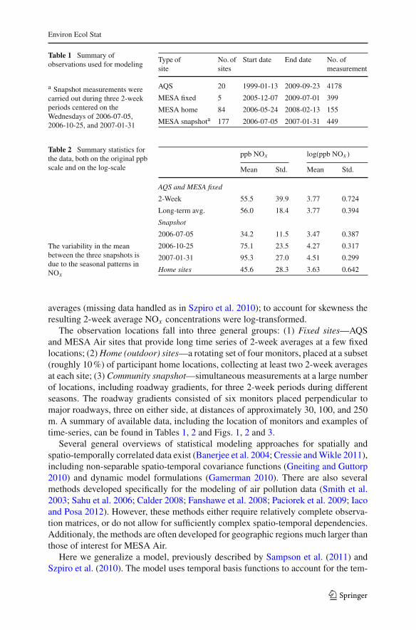
Table 1 Summary ofobservations used for modeling

a Snapshot measurements werecarried out during three 2-weekperiods centered on theWednesdays of 2006-07-05,2006-10-25, and 2007-01-31

Type ofsite

No. ofsites

Start date End date No. ofmeasurement

AQS 20 1999-01-13 2009-09-23 4178

MESA fixed 5 2005-12-07 2009-07-01 399

MESA home 84 2006-05-24 2008-02-13 155

MESA snapshota 177 2006-07-05 2007-01-31 449

Table 2 Summary statistics forthe data, both on the original ppbscale and on the log-scale

The variability in the meanbetween the three snapshots isdue to the seasonal patterns inNOx

ppb NOx log(ppb NOx )

Mean Std. Mean Std.

AQS and MESA fixed

2-Week 55.5 39.9 3.77 0.724

Long-term avg. 56.0 18.4 3.77 0.394

Snapshot

2006-07-05 34.2 11.5 3.47 0.387

2006-10-25 75.1 23.5 4.27 0.317

2007-01-31 95.3 27.0 4.51 0.299

Home sites 45.6 28.3 3.63 0.642

averages (missing data handled as in Szpiro et al. 2010); to account for skewness theresulting 2-week average NOx concentrations were log-transformed.

The observation locations fall into three general groups: (1) Fixed sites—AQSand MESA Air sites that provide long time series of 2-week averages at a few fixedlocations; (2) Home (outdoor) sites—a rotating set of four monitors, placed at a subset(roughly 10 %) of participant home locations, collecting at least two 2-week averagesat each site; (3) Community snapshot—simultaneous measurements at a large numberof locations, including roadway gradients, for three 2-week periods during differentseasons. The roadway gradients consisted of six monitors placed perpendicular tomajor roadways, three on either side, at distances of approximately 30, 100, and 250m. A summary of available data, including the location of monitors and examples oftime-series, can be found in Tables 1, 2 and Figs. 1, 2 and 3.

Several general overviews of statistical modeling approaches for spatially andspatio-temporally correlated data exist (Banerjee et al. 2004; Cressie and Wikle 2011),including non-separable spatio-temporal covariance functions (Gneiting and Guttorp2010) and dynamic model formulations (Gamerman 2010). There are also severalmethods developed specifically for the modeling of air pollution data (Smith et al.2003; Sahu et al. 2006; Calder 2008; Fanshawe et al. 2008; Paciorek et al. 2009; Iacoand Posa 2012). However, these methods either require relatively complete observa-tion matrices, or do not allow for sufficiently complex spatio-temporal dependencies.Additionaly, the methods are often developed for geographic regions much larger thanthose of interest for MESA Air.

Here we generalize a model, previously described by Sampson et al. (2011) andSzpiro et al. (2010). The model uses temporal basis functions to account for the tem-

123

Environ Ecol Stat

MESA monitoring

Date

Loca

tion

050

100

150

200

250

2000 2002 2004 2006 2008 2010

AQS sitesMESA snapshotMESA fixedMESA home

Fig. 1 Schematic image of the data available for analysis. Each measurement is represented by a pointin space and time. AQS provides temporally rich observations at 20 locations. During the second half ofour modeling period, additional temporally rich data are provided by 5 MESA fixed sites. Spatial data areprovided by the three MESA snapshot campaigns, which monitored a total of 177 locations at three timepoints, and by MESA home sites that consists of four monitors alternating among 84 locations

Fig. 2 Map illustrating the location of our measurements. The collocated AQS and MESA fixed site arenorth of the Lynwood AQS site; the MESA fixed site is partially obscured by the AQS sites

poral variability in data. To account for spatial variability in the temporal structure(see Fig. 3), the basis functions are modulated by spatially varying coefficients. Thecoefficients are modeled using universal kriging, where the linear trend contains Geo-

123

Environ Ecol Stat

Glendora 60370016

Date

NO

x (lo

g pp

b)

ObservationsFitted smooth trendlog(Caline+1)

Lynwood 60371301

Date

NO

x (lo

g pp

b)

Costa Mesa 60590007

Date

NO

x (lo

g pp

b)

01

23

45

60

12

34

56

01

23

45

60

12

34

56

A Home close to Lynwood 60371301

Date

NO

x (lo

g pp

b)

2000 2002 2004 2006 2008 2010

2000 2002 2004 2006 2008 2010

2000 2002 2004 2006 2008 2010

2000 2002 2004 2006 2008 2010

Fig. 3 Example time series of log-transformed 2-week average NOx concentrations at three AQS monitorsand one home site in the Los Angeles area. The fit of our smooth temporal basis functions to the data, andthe transformed Caline predictions are also shown. For the home site we have used the smooth temporal fitat the closest AQS monitor

123

Environ Ecol Stat

graphic Information System (GIS) covariates. The use of GIS covariates is termed“land use” regression (LUR) (Jerrett et al. 2005; Hoek et al. 2008). Covariates usedfor the Los Angeles NOx data are: (1) distance to a major road, i.e., census feature classcode A1–A3 (distances truncated to be ≥10 m and log-transformed), (2) distance to aA1 road (≥10 m, log-transformed), (3) total length of A1 and A2 roads in a circularbuffer with 300 m radius, (4) total length of A3 roads in a 50 m buffer, (5) distance tocoast (truncated to be ≤15 km), and (6) average population density in a 2 km buffer.Here census feature class code A1 roads refer to interstates and other limited accesshighways; A2 are primary roads without limited access; and A3 are secondary roads,e.g. state highways (see pp. 3–27 in US Census Bureau 2002). Available covariatesare described in Cohen et al. (2009); selection of covariates is presented in Merceret al. (2011). Having used spatially varying temporal basis functions to account fortemporal variability (see (2) in Sect. 2 for details), the residuals are assumed to consistof mean zero spatially dependent, but temporally uncorrelated fields (Sampson et al.2011; Szpiro et al. 2010).

Deterministic numerical models that provide predictions of air pollution offeran alternative to statistical modeling (Appel et al. 2008). However, comparisonsbetween measurements and air quality model output show varied prediction per-formance (Appel et al. 2008; Hogrefe et al. 2006), and an alternative is to com-bine model output with observations. In contrast to existing studies (Fuentes andRaftery 2005; Berrocal et al. 2010), which combine observations with output fromgrid-based models, we have here opted to combine our observations with the out-put from a point prediction model (Caline3QHCR, Eckhoff and Braverman 1995,hereafter called Caline). Given locations of major sources and local meteorol-ogy Caline uses a dispersion model to predict how nonreactive pollutants travelwith the wind, providing hourly estimates of air pollution at distinct points. TheCaline predictions used here are based on estimates of traffic density on majorroads in the Los Angeles area (see Wilton et al. 2010; Lindström et al. 2011, fordetails).

The main contributions of this paper are: (1) extending the model presented inSzpiro et al. (2010) to include spatio-temporal covariates; (2) applying the modelto the MESA Air NOx dataset to generate predictions for Los Angeles; (3) evaluat-ing the model’s ability to predict long term averages using a cross-validation strat-egy that accounts for the complex MESA Air monitoring design and that allowsus focus on spatial predictive ability by accounting for temporal effects; (4) inves-tigating the benefit of Caline as a spatio-temporal covariate and Caline’s abilityto replace traditional LUR covariates; and (5) reducing the computational bur-den of the model and evaluating how the computational burden scales with thenumber of observations. The model presented here has been implemented in anR package, SpatioTemporal, which is available from http://cran.r-project.org/package=SpatioTemporal.

The model is presented in Sect. 2. Computational considerations and parameterestimation are discussed in Sect. 3. Model validation, including considerations for theunbalanced dataset, is presented in Sect. 4. In Sect. 5 we apply the model to NOx datafrom Los Angeles, and investigate the contribution from Caline. Section 6 concludeswith a discussion.

123

Environ Ecol Stat

2 Model

We let C(s, t) denote the observed concentration of NOx at location s and time t andtake y(s, t) = log C(s, t). N denotes the total number of observations; n the numberof observation locations; and T the number of observation time points. Due to ourunbalanced sampling, N � nT . Our goal is to predict concentrations at unobservedlocations and/or times. We denote these unknown values by C∗(s, t). For convenienceimportant notation is summarized in Table 3.

The spatio-temporal process is decomposed into

y(s, t) = μ(s, t) + ν(s, t), (1)

where μ(s, t) is the mean process and ν(s, t) is the space-time residual process.The mean process is modeled as

μ(s, t) =L∑

l=1

γlMl(s, t) +m∑

i=1

βi (s) fi (t), (2)

where Ml(s, t) are spatio-temporal covariates with coefficients γl ; { fi (t)}mi=1 is a set

of smooth temporal basis functions, with f1(t) ≡ 1 and f2(t), . . . , fm(t) having mean

Table 3 Important notation andsymbols

Symbol Meaning

C(s, t) Observed 2-week average concentrations

C∗(s, t) Unobserved 2-week average concentrations

y(s, t) log C(s, t)

μ(s, t) Mean field part of y(s, t)

ν(s, t) Space-time residual part of y(s, t)

fi (t) Smooth temporal basis functions

βi (s) Spatially varying regression coefficients, weighingthe i th temporal trends differently at each site

Xi Land use regression (LUR) basis functions for thespatially varying regression coefficients in βi (s)

αi Regression coefficients for the i th LUR-basis

Ml (s, t) Spatio-temporally varying covariates

γl Regression coefficient for the spatio-temporallyvarying covariates

N No. of observations

T No. of observed time-points

n No. of observed sites

nt No. of observations at time t . Note thatN =∑T

t=1 nt and nt ≤ n ∀tm No. of temporal basis functions (incl. intercept)

L No. of spatio-temporal model outputs

pi No. of LUR-basis functions for the i thtemporal-basis function (incl. intercept)

123

Environ Ecol Stat

zero; and the βi (s) are spatially varying coefficients for the temporal trends. Typicallythe number of basis functions, m, will be small. The basis functions are derived assmoothed singular vectors using observations at the fixed sites; the basis functions aretreated as fixed and known for the modeling (see Fuentes et al. 2006; Szpiro et al.2010; Sampson et al. 2011, for details).

We model the spatial fields of βi -coefficients using universal kriging (Cressie 1993).The trend in the kriging is constructed as a linear regression on (geographic) covariates.The spatial dependence structure is provided by a set of covariance matrices, Σβi (θi ),parameterized by θi . The resulting models for the β-fields are

βi (s) ∈ N(Xiαi ,Σβi (θi )

)for i = 1, . . . , m, (3)

where Xi are n × pi design matrices, αi are pi × 1 matrices of regression coefficients,and Σβi (θi ) are n × n covariance matrices. We assume the βi (s) fields are, a priori,independent of each other.

The residual space-time process is modeled using mean zero Gaussian fields thatare temporally independent, but spatially dependent

ν(s, t) ∈ N(0,Σ t

ν(θν))

for t = 1, . . . , T ; (4)

the size of each covariance matrix, Σ tν(θν), is given by the numbers of observations,

nt , at time t . The covariance matrices depend on parameters, θν . Note that only thenumber of elements in Σ t

ν(θν), not the parametric functional form, varies with t . Thecovariance matrices in (3) and (4) are not required to share a common covariancemodel, allowing for a very flexible model.

The parameters of the model consist of: regression parameters for the spatio-temporal and geographic covariates, γ = (γ1, . . . , γL) and α = (α

1 , . . . , αm );

covariance parameters for the βi -fields, θB = (θ1, . . . , θm); and covariance parametersof the spatio-temporal residuals, θν . To simplify notation we collect the covarianceparameters into Ψ = (θ1, . . . , θm, θν).

Combining (1) and (2) our model becomes

y(s, t) =L∑

l=1

γlMl(s, t) +m∑

i=1

βi (s) fi (t) + ν(s, t). (5)

Following Szpiro et al. (2010), we introduce the N × 1-vectors Y = y(s, t) andV = ν(s, t) by stacking the elements into single vectors varying first s and thent ; a mn × 1-vector B = (β1(s), . . . , βm(s)); and a sparse N × mn-matrixF = ( fst,is′) with elements

fst,is′ ={

fi (t) s = s′0 otherwise.

To accommodate the spatio-temporal covariates we also introduce a N × L-matrix M,with each row containing covariates for the space-time location of the correspondingrow in Y . Using these matrices we rewrite (5) as

123

Environ Ecol Stat

Y = Mγ + F B + V, (6)

where B ∈ N (Xα,ΣB(θB)) and V ∈ N (0,Σν(θν)); X,ΣB(θB), and Σν(θν)

are block diagonal matrices with diagonal blocks {Xi }mi=1 ,

{Σβi (θi )

}mi=1, and

{Σ t

ν(θν)}T

t=1 respectively. Noting that (6) is a linear combinations of independentGaussians we introduce the matrices

X̃ = [M F X]

and Σ̃(Ψ ) = Σν(θν) + FΣB(θB)F, (7)

and write the distribution of Y as

[Y |Ψ, γ ,α] ∈ N(

X̃

[γ

α

], Σ̃(Ψ )

). (8)

3 Computational considerations

Parameter estimates can now be obtained by maximizing the likelihood of (8), using asuitable optimisation algorithm (e.g. L-BFGS-B, see Byrd et al. 1995). However, forlarge datasets estimation using naïve maximum likelihood (ML) takes considerabletime. There are two considerations for reducing the estimation time: (1) reducing thenumber of parameters, and (2) utilizing the block structure of Σν(θν) and ΣB(θB) toreduce the computational burden.

Replacing γ and α with their generalised least squares estimates (see Lindström etal. 2011, for details) gives the profile likelihood of (8)

2lPROF(Ψ |Y ) = −N log(2π) − log∣∣Σ̃(Ψ )

∣∣ − Y Σ̃−1(Ψ )Y

+Y Σ̃−1(Ψ )X̃(

X̃Σ̃−1(Ψ )X̃)−1

X̃Σ̃−1(Ψ )Y. (9)

To utilize the block diagonal structure of Σν(θν) and ΣB(θB) we rewrite (9) as

2lPROF(Ψ |Y ) = − log |Σν(θν)| − log |ΣB(θB)| − log∣∣∣Σ−1

B|Y (Ψ )

∣∣∣ − Y Σ̂(Ψ )Y

+Y Σ̂(Ψ )M(MΣ̂(Ψ )M

)−1MΣ̂(Ψ )Y + const. (10)

where const. does not depend on Ψ , and

Σ−1B|Y (Ψ ) = Σ−1

B (θB) + FΣ−1ν (θν)F, (11a)

Σ−1α|Y (Ψ ) = XΣ−1

B (θB)X − XΣ−1B (θB)ΣB|Y (Ψ )Σ−1

B (θB)X, (11b)

Σ̂(Ψ ) = Σ−1ν (θν) − Σ−1

ν (θν)FΣB|Y (Ψ )FΣ−1ν (θν)

−[Σ−1

ν (θν)FΣB|Y (Ψ )Σ−1B (θB)XΣα|Y (Ψ ) (11c)

XΣ−1B (θB)ΣB|Y (Ψ )FΣ−1

ν (θν)

].

123

Environ Ecol Stat

Computer time for evaluation of the profile log−likelihood

Number of observations

Tim

e (s

)

50004000300020001000

0.05

0.5

550

Naive, 1 to 286 locationsOptimised, 1 to 50 locationsOptimised, 51 to 100 locationsOptimised, 101 to 200 locationsOptimised, 201 to 286 locations

Fig. 4 Comparison of the time needed for one evaluation of the naïve profile likelihood (9) and simplifiedversion (10). The full dataset, 5182 observations from 286 locations and 280 time points, was divided intosmaller pieces by dropping either locations and/or time-points to examine how fast the evaluation timewould grow as the dataset was expanded. Evaluation time for the full likelihood grows as N 2.8 (the fitted

line) close to the expected theoretical value of O(

N 3)

. For a fixed number of locations evaluation time

for the simplified version grows considerably slower than N 3

Proof of equality between (9) and (10) is given in “Appendix”.At a first glance it is not obvious that (10) offers any computational advantages over

(9). The matrix Σ̃(Ψ ) in (9) is a dense N × N -matrix, implying that the computationaleffort of calculating log

∣∣Σ̃(Ψ )∣∣ grows at a rate of O (

N 3); the corresponding term in

(10),

log |Σν(θν)| + log |ΣB(θB)| + log∣∣∣Σ−1

B|Y (Ψ )

∣∣∣ ,

consists of the determinant of two block diagonal matrices and the determinant of adense mn × nm-matrix. The computational effort for the three components scalesare O (∑

t n3t

),O (

mn3), and O (

m3n3). For our data the term requiring O (

m3n3)

computer time will be the most time consuming. Due to the long time period coveredand the few temporal basis functions needed we have mn � N , implying that (10)should be considerably faster to evaluate than (9). With a more balanced samplingdesign the term requiring O (∑

t n3t

)is likely to dominate. Since

∑t n3

t <(∑

t nt)3 =

N 3, (10) is still faster to evaluate than (9). Similar arguments can be made for the restof the terms in the log-likelihood, and the overall computational cost of (9) growsas O (

N 3), compared to O (

m3n3)

or O (∑t n3

t

)for (10). As an example, evaluating

the likelihood once for our 5181 measurements in Los Angeles takes 92 s using (9),compared to 2.5 s for (10) (using an Intel Xeon E5410 processor). A comparison ofevaluation times is presented in Fig. 4. The figure illustrates the slower increase inevaluation time as a function of the number of observations for (10) compared to (9);

123

Environ Ecol Stat

it also shows the “jumps” in evaluation time for (10) when the number of locationsincrease.

The model (5) can also been seen as a multi-level mixed effects model (seee.g. Ch. 2 in Pinheiro and Bates 2009); this formulation is unlikely to offer anycomputational gains compared to the approach above. Alternatively, recent devel-opments in modelling of large datasets could be used to improve computationalefficiency. Examples include Gaussian Markov Random Fields (Lindgren et al.2011), predictive process (Banerjee et al. 2008) and, fixed rank kriging (Cressieand Johannesson 2008); these have all been extended to spatio-temporal data(Cameletti et al. 2013; Finley et al. 2012; Kang et al. 2010). However, theseextensions are, essentially, time dynamical models and do not allow for the com-plex structure, with temporal basis functions, in (2). For composite likelihoodmethods (Stein et al. 2004) it is non-trivial to construct blocking strategies inspace and time that account for the dependencies induced by the temporal basisfunctions.

4 Model validation

Having obtained estimates for the unknown parameters the next step is to predict con-centrations at unobserved locations and times. Given parameter estimates predictionsand prediction uncertainties for the log-concentrations, y∗(s, t), are obtained as con-ditional expectations and variances for a multivariate Gaussian (8). Unobserved NOx

concentrations are then obtained as C∗(s, t) = exp y∗(s, t), and validation is basedon the NOx -data.

We assess the predictive accuracy of our model using cross-validation, takinginto account the challenges presented by the unbalanced structure of our obser-vations. The primary interest of MESA Air is the long term average exposure,leaving us with the problem of trying to validate the spatial predictions of longterm averages based, in most cases, on a few observations at each location. Onlya few sites (the 25 fixed sites) have time-series long enough for us to computelong-term averages; additionally, the fixed sites have less heterogeneity in theirsurrounding environment but larger spatial spread than the remaining observationlocations.

To make the fullest use of available data we employ three different cross-validationstrategies: (1) leave-one-out cross-validation for the fixed sites, (2) 10-fold cross-validation for the community snapshots (ensuring not to split road gradients betweengroups); and (3) 10-fold cross-validation for the home sites. For each of the scenariosabove, all remaining data are used to estimate parameters and to predict at the left outlocations. Given the predictions and prediction variances we compute the coverage of95 % prediction intervals, the root mean squared error (RMSE) and the correspondingcross-validated R2.

For the first cross-validation approach we validate the model by comparing pre-dicted and observed concentrations, as well as the predicted and observed long-termaverage concentration at each location. The long-term averages (both true and pre-dicted) are computed by summation over only those time points for which we haveobservations, followed by division by the number of terms in the sum,

123

Environ Ecol Stat

C∗(s) =∑

t∈{τ : ∃y(s,τ )}

exp(y∗(s, t))

|{τ : ∃y(s, τ )}| .

The cross-validated R2’s are computed as (Szpiro et al. 2011a)

R2 = max

(0, 1 − RMSE2

Var(C(s))

). (12)

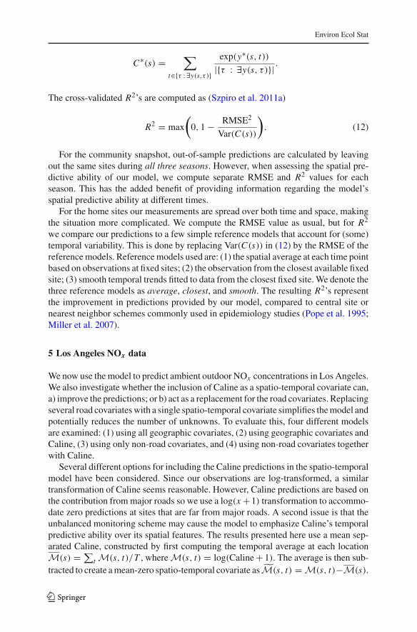
For the community snapshot, out-of-sample predictions are calculated by leavingout the same sites during all three seasons. However, when assessing the spatial pre-dictive ability of our model, we compute separate RMSE and R2 values for eachseason. This has the added benefit of providing information regarding the model’sspatial predictive ability at different times.

For the home sites our measurements are spread over both time and space, makingthe situation more complicated. We compute the RMSE value as usual, but for R2

we compare our predictions to a few simple reference models that account for (some)temporal variability. This is done by replacing Var(C(s)) in (12) by the RMSE of thereference models. Reference models used are: (1) the spatial average at each time pointbased on observations at fixed sites; (2) the observation from the closest available fixedsite; (3) smooth temporal trends fitted to data from the closest fixed site. We denote thethree reference models as average, closest, and smooth. The resulting R2’s representthe improvement in predictions provided by our model, compared to central site ornearest neighbor schemes commonly used in epidemiology studies (Pope et al. 1995;Miller et al. 2007).

5 Los Angeles NOx data

We now use the model to predict ambient outdoor NOx concentrations in Los Angeles.We also investigate whether the inclusion of Caline as a spatio-temporal covariate can,a) improve the predictions; or b) act as a replacement for the road covariates. Replacingseveral road covariates with a single spatio-temporal covariate simplifies the model andpotentially reduces the number of unknowns. To evaluate this, four different modelsare examined: (1) using all geographic covariates, (2) using geographic covariates andCaline, (3) using only non-road covariates, and (4) using non-road covariates togetherwith Caline.

Several different options for including the Caline predictions in the spatio-temporalmodel have been considered. Since our observations are log-transformed, a similartransformation of Caline seems reasonable. However, Caline predictions are based onthe contribution from major roads so we use a log(x +1) transformation to accommo-date zero predictions at sites that are far from major roads. A second issue is that theunbalanced monitoring scheme may cause the model to emphasize Caline’s temporalpredictive ability over its spatial features. The results presented here use a mean sep-arated Caline, constructed by first computing the temporal average at each locationM(s) = ∑

t M(s, t)/T , where M(s, t) = log(Caline + 1). The average is then sub-tracted to create a mean-zero spatio-temporal covariate as M̃(s, t) = M(s, t)−M(s).

123

Environ Ecol Stat

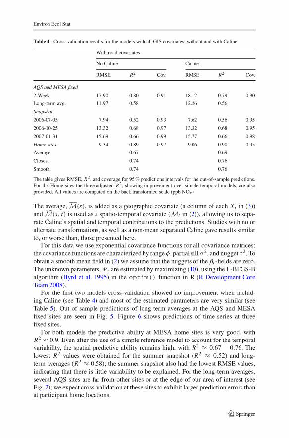
Table 4 Cross-validation results for the models with all GIS covariates, without and with Caline

With road covariates

No Caline Caline

RMSE R2 Cov. RMSE R2 Cov.

AQS and MESA fixed

2-Week 17.90 0.80 0.91 18.12 0.79 0.90

Long-term avg. 11.97 0.58 12.26 0.56

Snapshot

2006-07-05 7.94 0.52 0.93 7.62 0.56 0.95

2006-10-25 13.32 0.68 0.97 13.32 0.68 0.95

2007-01-31 15.69 0.66 0.99 15.77 0.66 0.98

Home sites 9.34 0.89 0.97 9.06 0.90 0.95

Average 0.67 0.69

Closest 0.74 0.76

Smooth 0.74 0.76

The table gives RMSE, R2, and coverage for 95 % predictions intervals for the out-of-sample predictions.For the Home sites the three adjusted R2, showing improvement over simple temporal models, are alsoprovided. All values are computed on the back transformed scale (ppb NOx )

The average, M(s), is added as a geographic covariate (a column of each Xi in (3))and M̃(s, t) is used as a spatio-temporal covariate (Ml in (2)), allowing us to sepa-rate Caline’s spatial and temporal contributions to the predictions. Studies with no oralternate transformations, as well as a non-mean separated Caline gave results similarto, or worse than, those presented here.

For this data we use exponential covariance functions for all covariance matrices;the covariance functions are characterized by range φ, partial sill σ 2, and nugget τ 2. Toobtain a smooth mean field in (2) we assume that the nuggets of the βi -fields are zero.The unknown parameters, Ψ , are estimated by maximizing (10), using the L-BFGS-Balgorithm (Byrd et al. 1995) in the optim() function in R (R Development CoreTeam 2008).

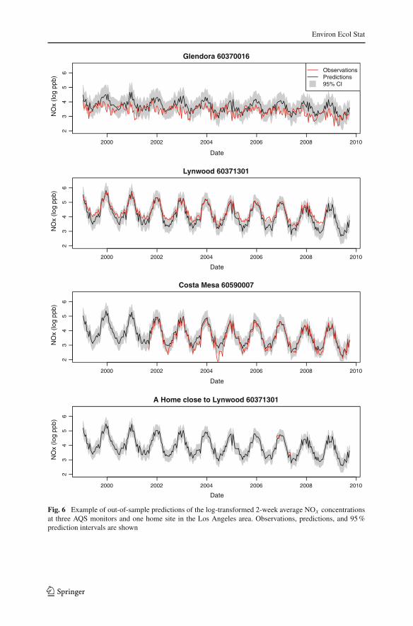
For the first two models cross-validation showed no improvement when includ-ing Caline (see Table 4) and most of the estimated parameters are very similar (seeTable 5). Out-of-sample predictions of long-term averages at the AQS and MESAfixed sites are seen in Fig. 5. Figure 6 shows predictions of time-series at threefixed sites.

For both models the predictive ability at MESA home sites is very good, withR2 ≈ 0.9. Even after the use of a simple reference model to account for the temporalvariability, the spatial predictive ability remains high, with R2 ≈ 0.67 − 0.76. Thelowest R2 values were obtained for the summer snapshot (R2 ≈ 0.52) and long-term averages (R2 ≈ 0.58); the summer snapshot also had the lowest RMSE values,indicating that there is little variability to be explained. For the long-term averages,several AQS sites are far from other sites or at the edge of our area of interest (seeFig. 2); we expect cross-validation at these sites to exhibit larger prediction errors thanat participant home locations.

123

Environ Ecol Stat

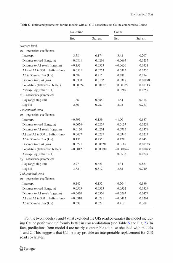
Table 5 Estimated parameters for the models with all GIS covariates: no Caline compared to Caline

No Caline Caline

Est. Std. err. Est. Std. err.

Average level

α1—regression coefficients

Intercept 3.78 0.174 3.42 0.207

Distance to road (log10 m) −0.0801 0.0236 −0.0665 0.0237

Distance to A1 roads (log10 m) −0.152 0.0323 −0.0630 0.0431

A1 and A2 in 300 m buffers (km) 0.0501 0.0253 0.0315 0.0256

A3 in 50 m buffers (km) 0.689 0.215 0.781 0.214

Distance to coast (km) 0.0330 0.0102 0.0318 0.00990

Population (1000/2 km buffer) 0.00324 0.00117 0.00335 0.00113

Average log(Caline + 1) 0.0789 0.0259

θ1—covariance parameters

Log range (log km) 1.86 0.388 1.84 0.384

Log sill −2.86 0.287 −2.92 0.283

1st temporal trend

α2—regression coefficients

Intercept −0.793 0.139 −1.00 0.187

Distance to road (log10 m) 0.00244 0.0259 0.0137 0.0254

Distance to A1 roads (log10 m) 0.0120 0.0274 0.0715 0.0379

A1 and A2 in 300 m buffers (km) 0.0437 0.0227 0.0345 0.0214

A3 in 50 m buffers (km) 0.136 0.255 0.178 0.245

Distance to coast (km) 0.0221 0.00720 0.0188 0.00753

Population (1000/2 km buffer) −0.00127 0.000782 −0.000949 0.000735

Average log(Caline + 1) 0.0533 0.0227

θ2—covariance parameters

Log range (log km) 2.77 0.621 3.34 0.831

Log sill −3.82 0.512 −3.55 0.740

2nd temporal trend

α3—regression coefficients

Intercept −0.142 0.132 −0.204 0.189

Distance to road (log10 m) 0.0503 0.0333 0.0532 0.0329

Distance to A1 roads (log10 m) −0.0430 0.0326 −0.0263 0.0479

A1 and A2 in 300 m buffers (km) −0.0310 0.0281 −0.0412 0.0264

A3 in 50 m buffers (km) 0.338 0.322 0.412 0.309

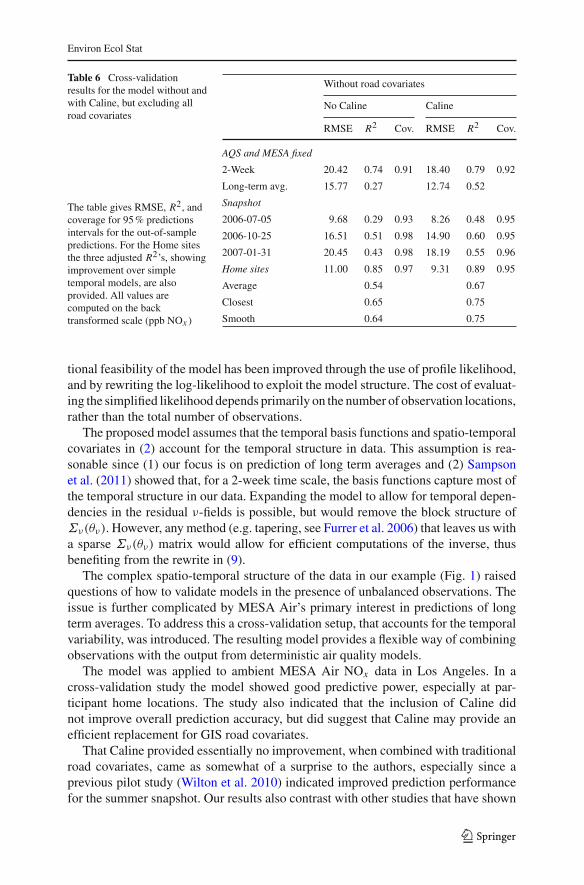
For the two models (3 and 4) that excluded the GIS road covariates the model includ-ing Caline performed uniformly better in cross-validation (see Table 6 and Fig. 5). Infact, predictions from model 4 are nearly comparable to those obtained with models1 and 2. This suggests that Caline may provide an interpretable replacement for GISroad covariates.

123

Environ Ecol Stat

Table 5 continued

No Caline Caline

Est. Std. err. Est. Std. err.

Distance to coast (km) 0.0130 0.00548 0.0121 0.00581

Population (1000/2 km buffer) −0.0000833 0.000924 0.0000423 0.000896

Average log(Caline + 1) 0.0185 0.0290

θ3—covariance parameters

Log range (log km) 2.40 0.646 2.68 0.724

Log sill −4.78 0.436 −4.70 0.515

γ

Mean centered log(Caline + 1) 0.0677 0.0151

θν

Log range (log km) 4.39 0.0938 4.38 0.0935

Log sill −3.25 0.0617 −3.25 0.0614

Log nugget −4.29 0.0415 −4.30 0.0418

Parameter values and standard errors based on the observed information matrix are given

With road covariates

observed

CV

pre

dict

ions

0 20 40 60 80

020

4060

80

0 20 40 60 80

Without road covariates

observed

CV

pre

dict

ions

No Caline

3km Caline

020

4060

80

Fig. 5 Out-of-sample predictions for the long-term averages at the AQS and MESA fixed sites. Resultsfor the model both including the road covariates (left) and without the road covariates (right) are given; forboth cases predictions without and with Caline are shown

In all four cases uncertainty estimates are reasonable, with the coverage for 95 %prediction intervals varying from 90 to 99 %.

6 Discussion

In this paper we have expanded the spatio-temporal framework introduced bySampson et al. (2011) and Szpiro et al. (2010) to allow for spatio-temporally varyingcovariates, such as the output from a deterministic air pollution model. The computa-

123

Environ Ecol Stat

Glendora 60370016

Date

NO

x (lo

g pp

b)

ObservationsPredictions95% CI

Lynwood 60371301

Date

NO

x (lo

g pp

b)

Costa Mesa 60590007

Date

NO

x (lo

g pp

b)

23

45

62

34

56

23

45

62

34

56

A Home close to Lynwood 60371301

Date

NO

x (lo

g pp

b)

2000 2002 2004 2006 2008 2010

2000 2002 2004 2006 2008 2010

2000 2002 2004 2006 2008 2010

2000 2002 2004 2006 2008 2010

Fig. 6 Example of out-of-sample predictions of the log-transformed 2-week average NOx concentrationsat three AQS monitors and one home site in the Los Angeles area. Observations, predictions, and 95 %prediction intervals are shown

123

Environ Ecol Stat

Table 6 Cross-validationresults for the model without andwith Caline, but excluding allroad covariates

The table gives RMSE, R2, andcoverage for 95 % predictionsintervals for the out-of-samplepredictions. For the Home sitesthe three adjusted R2’s, showingimprovement over simpletemporal models, are alsoprovided. All values arecomputed on the backtransformed scale (ppb NOx )

Without road covariates

No Caline Caline

RMSE R2 Cov. RMSE R2 Cov.

AQS and MESA fixed

2-Week 20.42 0.74 0.91 18.40 0.79 0.92

Long-term avg. 15.77 0.27 12.74 0.52

Snapshot

2006-07-05 9.68 0.29 0.93 8.26 0.48 0.95

2006-10-25 16.51 0.51 0.98 14.90 0.60 0.95

2007-01-31 20.45 0.43 0.98 18.19 0.55 0.96

Home sites 11.00 0.85 0.97 9.31 0.89 0.95

Average 0.54 0.67

Closest 0.65 0.75

Smooth 0.64 0.75

tional feasibility of the model has been improved through the use of profile likelihood,and by rewriting the log-likelihood to exploit the model structure. The cost of evaluat-ing the simplified likelihood depends primarily on the number of observation locations,rather than the total number of observations.

The proposed model assumes that the temporal basis functions and spatio-temporalcovariates in (2) account for the temporal structure in data. This assumption is rea-sonable since (1) our focus is on prediction of long term averages and (2) Sampsonet al. (2011) showed that, for a 2-week time scale, the basis functions capture most ofthe temporal structure in our data. Expanding the model to allow for temporal depen-dencies in the residual ν-fields is possible, but would remove the block structure ofΣν(θν). However, any method (e.g. tapering, see Furrer et al. 2006) that leaves us witha sparse Σν(θν) matrix would allow for efficient computations of the inverse, thusbenefiting from the rewrite in (9).

The complex spatio-temporal structure of the data in our example (Fig. 1) raisedquestions of how to validate models in the presence of unbalanced observations. Theissue is further complicated by MESA Air’s primary interest in predictions of longterm averages. To address this a cross-validation setup, that accounts for the temporalvariability, was introduced. The resulting model provides a flexible way of combiningobservations with the output from deterministic air quality models.

The model was applied to ambient MESA Air NOx data in Los Angeles. In across-validation study the model showed good predictive power, especially at par-ticipant home locations. The study also indicated that the inclusion of Caline didnot improve overall prediction accuracy, but did suggest that Caline may provide anefficient replacement for GIS road covariates.

That Caline provided essentially no improvement, when combined with traditionalroad covariates, came as somewhat of a surprise to the authors, especially since aprevious pilot study (Wilton et al. 2010) indicated improved prediction performancefor the summer snapshot. Our results also contrast with other studies that have shown

123

Environ Ecol Stat

improvement in air quality predictions by combining observations with output fromdeterministic models (Fuentes and Raftery 2005; Berrocal et al. 2010). These studiesdo not use any GIS covariates, but do use output from grid based models over largegeographic areas, often several states. These differences make it difficult to translatetheir results to our limited geographic areas and study design.

The overall prediction results are encouraging and indicate that the model will beable to provide the basis for high quality predicted exposures in MESA Air healthanalyses.

Acknowledgments Although the research described in this article has been funded wholly or in partby the United States Environmental Protection Agency through assistance agreement CR-834077101-0and grant RD831697 to the University of Washington, it has not been subjected to the Agency’s requiredpeer and policy review and therefore does not necessarily reflect the views of the Agency and no officialendorsement should be inferred. Travel for Johan Lindström has been paid by STINT (The Swedish Foun-dation for International Cooperation in Research and Higher Education) Grant IG2005-2047 and the RoyalPhysiographic Society in Lund.

Appendix: Proof of equivalence for the simplified likelihood

To prove the equivalence of the two likelihood forms (9) and (10) we need the follow-ing:

Lemma 1 If Σ1 and Σ2 are two nonsingular matrices of size n1-by-n1 and n2-by-n2respectively, and A is a n2-by-n1 matrix, then:

∣∣∣AΣ1 A + Σ2

∣∣∣ = |Σ1| |Σ2|∣∣∣Σ−1

1 + AΣ−12 A

∣∣∣ .

(Harville 1997, Thm. 18.1.1)

Lemma 2 The Woodbury identity (Harville 1997, Thm. 18.2.8): If A and B are twoinvertable matrices of size n-by-n and p-by-p respectively, and C is an arbitraryn-by-p matrix, then

(A + C BC)−1 = A−1 − A−1C

(B−1 + C A−1C

)−1C A−1.

Rearranging the terms and multiplying with A from both sides, Lemma 2 becomes

C(

B−1 + C A−1C)−1

C = A − A(

A + C BC)−1A. (13)

Lemma 3 The Searle identity (Harville 1997, Thm. 18.2.3): If A, B are matrices ofsize p-by-n and n-by-p respectively, I denotes identity matrices of appropriate size,and (I + AB) is nonsingular, then

(I + AB)−1 A = A (I + B A)−1 .

Lemma 4 Blockwise inversion (Harville 1997, Thm. 8.5.11): Let A, B, C, and D beblock matrices, with A and (D − C A−1 B) being nonsingular, then

123

Environ Ecol Stat

[A BC D

]−1

=[

A−1 + A−1 B(D − C A−1 B

)−1C A−1 −A−1 B

(D − C A−1 B

)−1

−(D − C A−1 B

)−1C A−1

(D − C A−1 B

)−1

].

To make the notation clearer we suppress the dependence on Ψ . Superscripts aboveequality signs denote the identities used in each step.

For the determinant in (9) we have

∣∣Σ̃∣∣ (7)=

∣∣∣Σν + FΣB F∣∣∣ Lem. 1&(11a)= |Σν | |ΣB |

∣∣∣Σ−1B|Y

∣∣∣ ,

proving equality with the determinants in (10).For the quadratic form in (9) we first note that

Σ̃−1 Lem. 2= Σ−1ν − Σ−1

ν FΣB|Y FΣ−1ν , (14a)

FΣ̃−1 F(13)= Σ−1

B − Σ−1B ΣB|Y Σ−1

B , (14b)

Σ̃−1 F(7)= (

I + Σ−1ν FΣB F)−1

Σ−1ν F

Lem. 3= Σ−1ν FΣB|Y Σ−1

B . (14c)

Using (14) we have that

Σ−1α|Y

(11b)& (14b)= XFΣ̃−1 F X (15a)

Σ̂(11c)&(14a)&(14c)= −Σ̃−1 F XΣα|Y XFΣ̃−1 + Σ̃−1. (15b)

For the quadratic form in (9) we have

Y Σ̃−1 X̃(

X̃Σ̃−1 X̃)−1

X̃Σ̃−1Y − Y Σ̃−1Y

(7)&(15a)= Y Σ̃−1 X̃

[Σ−1

α|Y MΣ̃−1ν F X

XFΣ̃−1ν M MΣ̃−1

ν M]−1

X̃Σ̃−1Y − Y Σ̃−1Y

Lem. 4&(15b)= Y Σ̃−1[

F XΣα|Y XF +(

I − F XΣα|Y XFΣ̃−1)

M(MΣ̂M)−1M(I − Σ̃−1 F XΣα|Y XF)]

Σ̃−1Y − Y Σ̃−1Y

= Y [(

Σ̃−1 − Σ̃−1 F XΣα|Y XFΣ̃−1)M(MΣ̂M)−1M

(Σ̃−1 − Σ̃−1 F XΣα|Y XFΣ̃−1

)

−(Σ̃−1 − Σ̃−1 F XΣα|Y XFΣ̃−1

)]Y

(15b)= Y Σ̂M(MΣ̂M

)−1MΣ̂Y − Y Σ̂Y,

showing that the quadratic forms in (9) and (10) are equal.

123

Environ Ecol Stat

References

Appel KW, Bhave PV, Gilliland AB, Sarwar G, Roselle SJ (2008) Evaluation of the community multiscaleair quality (CMAQ) model version 4.5: sensitivities impacting model performance; part II—particulatematter. Atmos Environ 42(24):6057–6066

Banerjee S, Carlin BP, Gelfand AE (2004) Hierarchical modeling and analysis for spatial data. Chapman& Hall/CRC, London

Banerjee S, Gelfand AE, Finley AO, Sang H (2008) Gaussian predictive process models for large spatialdata sets. J R Stat Soc Ser B 70:825–848

Basu R, Woodruff TJ, Parker JD, Saulnier L, Schoendorf KC (2000) Particulate air pollution and mortality:findings from 20 U.S. cities. N Engl J Med 343(24):1742–1749

Berrocal VJ, Gelfand AE, Holland DM (2010) A spatio-temporal downscaler for output from numericalmodels. J Agric Bio Environ Stat 15(2):176–197

Bild DE, Bluemke DA, Burke GL, Detrano R, Diez Roux AV, Folsom AR, Greenland P, Jacobs DR Jr,Kronmal R, Liu K, Nelson JC, O’Leary D, Saad MF, Shea S, Szklo M, Tracy RP (2002) Multi-ethnicstudy of atherosclerosis: objectives and design. Am J Epidemiol 156(9):871–881

Brauer M, Hoek G, van Vliet P, Meliefste K, Fischer P, Gehring U, Heinrich J, Cyrys J, Bellander T,Lewne M, Brunekreef B (2003) Estimating long-term average particulate air pollution concentrations:application of traffic indicators and geographic information systems. Epidemiology 14(2):228–239

Byrd R, Lu P, Nocedal J, Zhu C (1995) A limited memory algorithm for bound constrained optimization.SIAM J Sci Comput 16:1190–1208

Calder CA (2008) A dynamic process convolution approach to modeling ambient particulate matter con-centrations. Environmetrics 19(1):39–48

Cameletti M, Lindgren F, Simpson D, Rue H (2013) Spatio-temporal modeling of particulate matter con-centration through the SPDE approach. AStA Adv Stat Anal 97(2):109–131

Carroll RJ, Ruppert D, Stefanski LA, Crainiceanu CM (2006) Measurement error in nonlinear models: amodern perspective, 2nd edn. Chapman and Hall, CRC, London

Cohen MA, Adar SD, Allen RW, Avol E, Curl CL, Gould T, Hardie D, Ho A, Kinney P, Larson TV,Sampson PD, Sheppard L, Stukovsky KD, Swan SS, Liu LJS, Kaufman JD (2009) Approach to estimatingparticipant pollutant exposures in the multi-ethnic study of atherosclerosis and air pollution (MESA air).Environ Sci Technol 43(13):4687–4693

Cressie N (1993) Statistics for spatial data, revised edition. Wiley, LondonCressie N, Johannesson G (2008) Fixed rank kriging for very large spatial data sets. J R Stat Soc Ser B

70(1):209–226Cressie N, Wikle CK (2011) Statistics for spatio-temporal data. Wiley, LondonDe Iaco S, Posa D (2012) Predicting spatio-temporal random fields: some computational aspects. Comput

Geosci 41:12–24Dockery DW, Pope CA, Xu X, Spangler JD, Ware JH, Fay ME, Ferris BG, Speizer FE (1993) An association

between air pollution and mortality in six cities. N Engl J Med 329(24):1753–1759Eckhoff P, Braverman T (1995) Addendum to the user’s guide to CAL3QHC version 2.0 (CAL3QHCR

user’s guide). Technical report, US Environmental Protection Agency, Office of Air Quality Planningand Standards, Research Triangle Park, NC, USA

Fanshawe TR, Diggle PJ, Rushton S, Sanderson R, Lurz PWW, Glinianaia SV, Pearce MS, Parker L,Charlton M, Pless-Mulloli T (2008) Modelling spatio-temporal variation in exposure to particulatematter: a two-stage approach. Environmetrics 19(6):549–566

Finley AO, Banerjee S, Gelfand AE (2012) Bayesian dynamic modeling for large space-time datasets usinggaussian predictive processes. J Geogr Syst 14(1):29–47

Fuentes M, Raftery AE (2005) Model evaluation and spatial interpolation by Bayesian combination ofobservations with outputs from numerical models. Biometrics 61(1):34–45

Fuentes M, Guttorp P, Sampson PD (2006) Using transforms to analyze space-time processes. In: FinkenstädtB, Held L, Isham V (eds) Statistical methods for spatio-temporal systems. Chapman & Hall/CRC,London, pp 77–150

Furrer R, Genton MG, Nychka D (2006) Covariance tapering for interpolation of large spatial datasets. JComput Graph Stat 15(3):502–523

Gamerman D (2010) Dynamic spatial models including spatial time series. In: Gelfand AE, Diggle P,Guttorp P, Fuentes M (eds) Handbook of spatial statistics. Chapman & Hall/CRC, London, pp 437–448

123

Environ Ecol Stat

Gneiting T, Guttorp P (2010) Continuous parameter spatio-temporal processes. In: Gelfand AE, Diggle P,Guttorp P, Fuentes M (eds) Handbook of Spatial Statistics. Chapman & Hall/CRC, London, pp 427–436

Gryparis A, Paciorek CJ, Zeka A, Schwartz J, Coull BA (2009) Measurement error caused by spatialmisalignment in environmental epidemiology. Biostatistics 10(2):258–274

Harville DA (1997) Matrix algebra from a statistician’s perspective, 1st edn. Springer, BerlinHoek G, Beelen R, de Hoogh K, Vienneau D, Gulliver J, Fischer P, Briggs D (2008) A review of land-use

regression models to assess spatial variation of outdoor air pollution. Atmos Environ 42(3):7561–7578Hogrefe C, Porter P, Gego E, Gilliland A, Gilliam R, Swall J, Irwin J, Rao S (2006) Temporal features

in observed and simulated meteorology and air quality over the Eastern United States. Atmos Environ40(26):5041–5055

Jerrett M, Arain A, Kanaroglou P, Beckerman B, Potoglou D, Sahsuvaroglu T, Morrison J, Giovis C (2005)A review and evaluation of intraurban air pollution exposure models. J Expo Anal Environ Epidemiol15:185–204

Kang EL, Cressie N, Shi T (2010) Using temporal variability to improve spatial mapping with applicationto satellite data. Can J Stat 38(2):271–289

Kaufman JD, Adar SD, Allen RW, Barr RG, Budoff MJ, Burke GL, Casillas AM, Cohen MA, Curl CL,Daviglus ML, Roux AVD, Jacobs DR, Kronmal RA, Larson TV, Liu SLJ, Lumley T, Navas-AcienA, O’Leary DH, Rotter JI, Sampson PD, Sheppard L, Siscovick DS, Stein JH, Szpiro AA, Tracy RP(2012) Prospective study of particulate air pollution exposures, subclinical atherosclerosis, and clinicalcardiovascular disease: the multi-ethnic study of atherosclerosis and air pollution (MESA air). Am JEpidemiol 176(9):825–837

Lindgren F, Rue H, Lindström J (2011) An explicit link between Gaussian fields and Gaussian Markovrandom fields: the stochastic partial differential equation approach. J R Stat Soc Ser B 73(4):423–498

Lindström J, Szpiro AA, Sampson PD, Sheppard L, Oron A, Richards M, Larson T (2011) Incorporatingoutput from source dispersion models into the spatio-temporal modelling of outdoor pollutant concentra-tions. Technical report. Working paper 370, UW Biostatistics working paper series. http://www.bepress.com/uwbiostat/paper370

Mercer LD, Szpiro AA, Sheppard L, Lindström J, Adar SD, Allen RW, Avol EL, Oron AP, Larson T, Liu LJS,Kaufman JD (2011) Comparing universal kriging and land-use regression for predicting concentrationsof gaseous oxides of nitrogen (NOx ) for the multi-ethnic study of atherosclerosis and air pollution(MESA air). Atmos Environ 45(26):4412–4420

Miller KA, Sicovick DS, Sheppard L, Shepherd K, Sullivan JH, Anderson GL, Kaufman JD (2007)Long-term exposure to air pollution and incidence of cardiovascular events in women. N Engl J Med356(5):447–458

Paciorek CJ (2010) The importance of scale for spatial-confounding bias and precision of spatial regressionestimators. Stat Sci 25(1):107–125

Paciorek CP, Yanosky JD, Puett RC, Laden F, Suh HH (2009) Practical large-scale spatio-temporal modelingof particulate matter concentrations. Ann Stat 3(1):370–397

Pinheiro J, Bates D (2009) Mixed-effects models in S and S-PLUS. Statistics and computing. Springer,Berlin

Pope CA, Thun MJ, Namboodiri MM, Dockery DW, Evans JS, Speizer FE, Heath CW Jr (1995) Particulateair pollution as a predictor of mortality in a prospective study of U.S. adults. Am J Respir Crit Care Med151:669–674

Pope CA, Burnett RT, Thun MJ, Calle EE, Krewski D, Ito K, Thurston GD (2002) Lung cancer, car-diopulmonary mortality, and long-term exposure to fine particulate air pollution. J Am Med Assoc9(287):1132–1141

Puett RC, Hart JE, Yanosky JD, Paciorek CJ, Schwartz J, Suh H, Speizer FE, Laden F (2009) Chronic fineand coarse particulate exposure, mortality and coronary heart disease in the nurses’ health study. EnvironHealth Perspect 117:1697–1701

R Development Core Team (2008) R: a language and environment for statistical computing. R Foundationfor Statistical Computing, Vienna, Austria. http://www.R-project.org. ISBN 3-900051-07-0

Sahu SK, Gelfand AE, Holland D (2006) Spatio-temporal modeling of fine particulate matter. J Agric BioEnviron Stat 11(1):61–86

Sampson PD, Szpiro AA, Sheppard L, Lindström J, Kaufman JD (2011) Pragmatic estimation of a spatio-temporal air quality model with irregular monitoring data. Atmos Environ 45(36):6593–6606

Sheppard L, Burnett RT, Szpiro AA, Kim SY, Jerrett M, Pope CA III, Brunekreef B (2012) Confoundingand exposure measurement error in air pollution epidemiology. Air Qual Atmos Health 5(2):203–216

123

Environ Ecol Stat

Smith RL, Kolenikov S, Cox LH (2003) Spatio-temporal modeling of PM2.5 data with missing values. JGeophys Res 108(D24):9004

Stein ML, Chi Z, Welty LJ (2004) Approximating likelihoods for large spatial data sets. J R Stat Soc Ser B66(2):275–296

Szpiro AA, Sampson PD, Sheppard L, Lumley T, Adar S, Kaufman J (2010) Predicting intra-urban variationin air pollution concentrations with complex spatio-temporal dependencies. Environmetrics 21(6):606–631

Szpiro AA, Paciorek C, Sheppard L (2011a) Does more accurate exposure prediction necessarily improvehealth effect estimates? Epidemiology 22(5):680–685

Szpiro AA, Sheppard L, Lumley T (2011b) Efficient measurement error correction with spatially misaligneddata. Biostatistics 12(4):610–623

US Census Bureau (2002) UA census 2000 TIGER/line files technical documentation. Technical report,US Census Bureau, Washington, DC. https://www.census.gov/geo/www/tiger/tigerua/ua2ktgr.pdf

Wilton D, Szpiro AA, Gould T, Larson T (2010) Improving spatial concentration estimates for nitrogenoxides using a hybrid meteorological dispersion/land use regression model in Los Angeles, CA andSeattle. WA. Sci Total Environ 408(5):1120–1130

Author Biographies

Johan Lindström is Assistant Professor at the Centre for Mathematical Sciences at Lund University. Hereceived a M.Sc. in Engineering Physics in 2003 and a Ph.D. in Mathematical Statistics in 2008, both fromLund University. He did a PostDoc at University of Washington during 2009–2010. His current researchinterests include spatio-temporal modeling with applications to climate and environmental data, GaussianMarkov Random Fields, and general statistical applications in climate sciences. His a member of LundUniversity’s strategic research areas BECC (Biodiversity and Ecosystem services in a Changing Climate)and MERGE (ModElling the Regional and Global Earth system).

Adam A. Szpiro is Assistant Professor in the Department of Biostatistics at the University of Washing-ton. He received a B.A. in Mathematics from UC San Diego in 1993 and an Sc.M. and Ph.D. in AppliedMathematics from Brown University in 1994 and1999, respectively. He previously worked at MIT LincolnLaboratory in air defense and bioterrorism defense. His current research interests include spatio-temporalmodeling with applications to air pollution, measurement error correction in environmental epidemiology,and Bayesian methods for model-robust inference.

Paul D. Sampson is Research Professor of Statistics and Director of the Statistical Consulting programin the Department of Statistics at the University of Washington. He received an Sc.M. degree in AppliedMathematics from Brown University and a Ph.D. in Statistics from the University of Michigan. He has along history of research on spatio-temporal modeling of environmental data, beginning with the introduc-tion of the Sampson-Guttorp deformation model for nonstationary spatial covariance structure. Currentresearch focuses on collaborations with colleagues in environmental health science on applications in airpollution epidemiology.

Assaf P. Oron is a senior statistician at the Children’s Core for Biomedical Statistics at Seattle Chil-dren’s Research Institute. He holds a B.Sc. in physics from the Hebrew University, an M.Sc. in environ-mental science from the Weizmann Institute, and a Ph.D. in statistics from the University of Washington.Assaf has extensive experience in interdisciplinary research, combining scientific and statistical insight.His main methodological interest is dose-finding experiment design and analysis.

Mark Richards is an Applied Mathematics Master student at the University of Washington. He receivedBA degrees from the University of California, Berkeley, in Applied Mathematics and Statistics. He hasworked for the MESA Air study as a data manager and statistical modeler. His current research interestsare in the field of mathematical biology.

123

Environ Ecol Stat

Tim V. Larson is Professor in the Department of Civil and Environmental Engineering and in the Depart-ment of Occupational and Environmental Health Sciences at the University of Washington. Dr. Larsonholds a B.S. in Chemical Engineering from Lehigh University (1968), and an M.S.Ch.E. (1972) and Ph.D.(1976) from the University of Washington. His expertise is in characterization of urban air pollution, expo-sure assessment of airborne particles and gases, and source/receptor relationships of ambient air pollu-tants. Dr. Larson’s major focus in recent years has been on assessment of human exposure to outdoorgenerated air pollutants.

Lianne Sheppard is Professor of Biostatistics, and Environmental and Occupational Health Sciences atthe University of Washington. She received her Sc.M. and Ph.D. degrees in biostatistics from the JohnsHopkins University and University of Washington, respectively. Her research interests focus on statisticalmethods for environmental and occupational epidemiology and include study design and estimation ofenvironmental exposure effects. Currently she collaborates on several air pollution chort studies, includingMESA Air, a study funded by EPA to assess the effect of long-term air pollution exposure on subclinicalprogression of cardiovascular disease.

123