A Divergence Statistic for Industrial Localization

Tomoya Mori∗, Koji Nishikimi†and Tony E. Smith‡

January 31, 2005

Abstract

In this paper, we propose a statistical index of industrial localization based on Kullback-Leibler

divergence. This index is particularly well suited to cases where industrial data is only available at the

regional level. Unlike existing regional-level indices, our index can be employed to test the significance

of industrial localization relative to a hypothesized reference distribution of probable locations across

regions. In addition, one can test relative degrees of localization among industries. Finally, as with

all Kullback-Leibler divergence indices, our index can be decomposed into components representing

localization at various levels of spatial aggregation.

Keywords : Industrial localization, Kullback-Leibler divergence, Relative entropy, Large-sample analysis of local-

ization, Spatial decomposition of localization

JEL Classifications: C19, L60, R12

∗Institute of Economic Research, Kyoto University, Yoshida-Honmachi, Sakyo-ku, Kyoto, 606-8501 Japan. Email:mori@kier.kyoto-u.ac.jp. Phone: +81-75-753-7121. Fax: +81-75-753-7198.

†Institute of Developing Economies/JETRO, 3-2-2 Wakaba, Mihama-ku, Chiba, 261-8545 Japan. Email:nisikimi@ide.go.jp. Phone: +81-43-299-9672. Fax: +81-43-299-9763.

‡Department of Electrical and Systems Engineering, University of Pennsylvania, Philadelphia, PA 19104, USA. Email:tesmith@ssc.upenn.edu. Phone: +1-215-898-9647. Fax: +1-215-898-5020.

Acknowledgment

Earlier versions of this paper was presented at the 16th Meeting of the Applied Regional Science

Conference at Okayama University, December 1-2, 2002, the conference on the economics of cities at

London School of Economics, June 6-8, 2003, seminars at Osaka University and Osaka Prefecture Uni-

versity. We are grateful to conference/seminar participants for their constructive comments. We have

benefited greatly from discussions with Gilles Duranton, Vernon Henderson, Kazuhiko Kakamu, Yoshi-

hiko Nishiyama, Henry Overman, Akihisa Shibata, and two anonymous referees. This research has been

supported by The Murata Science Foundation, The Grant in Aid for Research (Nos. 09CE2002, 09730009,

13851002) of Ministry of Education, Science and Culture in Japan.

1 Introduction

In the past decade, a substantial number of empirical studies of industrial localization have appeared

in the literature.1 These studies suggest that industrial localization is far more ubiquitous than pre-

viously believed, and extends well beyond the classical agglomerations of industries exemplified by the

information-technology industry in Silicon Valley and automobile industry in Detroit. Moreover, the

degree of such localization varies across industries, and often tends to be more subtle than these classical

examples. However, most localization indices currently in use provide no clear statistical method for

detecting the presence of localization.2 Hence the central purpose of this paper is to develop an index of

localization that does provide such a statistical testing framework.3

The index we employ is based on the concept of Kullback-Leibler divergence (1951), and is here

designated as the D-index of industrial localization. In particular, a reference distribution of complete

spatial dispersion is formulated as a null hypothesis, and the D-index for each industry is computed as the

Kullback-Leibler divergence between the observed spatial distribution of establishments for that industry

and this reference distribution. Since higher values of D are taken to convey stronger evidence against

complete spatial dispersion, we interpret this to be evidence for localization in that industry. Within

this framework it is shown that under the null hypothesis of complete spatial dispersion, the D-index

is asymptotically normally distributed, and thus provides a natural statistical test for this hypothesis.

However, the more relevant question for our purposes focuses on the relative magnitude of D for different

industries. Hence the main application of this asymptotic normality property is to construct tests of

the differences between D-indices for separate industries, and thereby to conclude that industries with

significantly higher D-values are significantly more localized.4

Our null hypothesis of complete spatial dispersion for any industry is operationalized by postulating

that all feasible locations for establishments in that industry are equally likely. If the totality of these

locations is designated as the economic area within the given geographic area (see footnote 29), then

this hypothesis is formalized as a uniform probability distribution over economic area, representing the

probable location of a randomly sampled establishment within that industry. Unlike the more traditional

approach of using industrial aggregates as reference distributions [e.g., Ellison and Glaeser (1997) and

Krugman (1991)],5 this hypothesis of complete spatial dispersion is more directly related to existing

theories of economic agglomeration in terms of spatial proximity.6

Finally, it is well known that Kullback-Leibler divergence indices are decomposable with respect to

partitions of the sample space.7 In particular, the D-index can be decomposed with respect to the choice

of geographical units. This provides a way of measuring the spatial extent of industrial localization,

thereby suggesting the most appropriate geographic units for industrial localization analysis. While the

decomposability result itself is not new, its application to the localization index is new.8

1

The rest of the paper is organized as follows. In Section 2, we begin by defining our D-index for

industrial localization and highlight some of its major characteristics. In Section 3, we discuss large

sample properties of the D-index, and develop its asymptotic normality properties. In Section 4, these

results are applied to the case of Japan. Here the D-index is computed for Japanese industries and

compared with the traditional index of Ellison and Glaeser (1997). The paper concludes with a brief

discussion of directions for further research.

2 Measure of localization

In this section, we propose our new index of industrial localization and discuss its major aspects. We

start by laying out the formal framework for our analysis in Section 2.1. The D-index is then defined

in Section 2.2, and its interpretation in terms of likelihood ratios is given in Section 2.3. Finally, the

decomposition properties of the D-index are developed in Section 2.4.

2.1 Basic setting

Consider a finite set of industries, i ∈ I = {1, .., I}, located within a set of regions, r ∈ R = {1, .., R}.

Suppose that Nir denotes the total number of establishments of industry i in region r. Then the ob-

jective of the present analysis is to characterize the degree of geographic concentration or dispersion of

establishments among industries, as exhibited by the establishment location pattern (Nir : ir ∈ I×R).

The approach adopted here is to treat this establishment location pattern, Ni = (Nir : r ∈ R), of each

industry i as a random sample of size ni =PrNir from a larger statistical population of potential estab-

lishments. If pir denotes the probability that a randomly sampled establishment from industry i will be

located in region r, then our interest focuses on the relative degrees of spatial concentration exhibited by

each of these i-establishment distributions, pi = (pir : r ∈ R) , i ∈ I. It should be noted that the random

sampling assumption above implies that the locational decisions of individual establishments are treated

as statistically independent events. Of course this is at best an approximation to the actual dynamics of

successive locational decisions by establishments.9

To characterize the observed location pattern of establishments, we begin by formulating a probability

model of “complete spatial dispersion” and then consider the deviations of each distribution, pi, from this

benchmark model. Here it is postulated that a completely dispersed distribution for industry i is one in

which randomly sampled i-establishments are equally likely to be located anywhere within the economic

area, a, of the given regional system. If ar denotes the economic area of region r, then under complete

spatial dispersion the probability that a randomly sampled i-establishment will be located in region r is

2

given by the fraction:

p0r = ar/a , r ∈ R. (1)

Hence, this hypothesis of complete spatial dispersion is summarized by the probability distribution

p0 = (p0r : r ∈ R) (2)

which we now adopt as a benchmark against which to compare all i-establishment distributions, pi.

It should be noted at this point that alternative null hypotheses are possible in which the benchmark

distribution is, for example, based on the regional fractions of total establishments or employment levels

for all industries. The implications of these alternative choices are discussed more fully in Appendix A

below.

2.2 Definition of the D-index

How can we measure the deviation between the two distributions, pi and p0? While there are many possi-

ble measures of deviation between distributions,10 the most natural choice from a statistical viewpoint is

the Kullback-Leibler divergence between pi and p0.11 This divergence measure (also called as the relative

entropy of pi with respect to p0) is defined as follows:12

D(pi|p0) =P

r∈R pir ln

µpirp0r

¶. (3)

D(pi|p0) is well known to be nonnegative, and to achieve its minimum uniquely at zero when pi =

p0. Moreover, its local maxima are achieved precisely at the degenerate distributions in which all i-

establishments are concentrated in a single region (i.e., with pir = 1 for some r ∈ R).13 Hence it is

natural to regard values of D(pi|p0) for each industry i as reflecting its degree of localization. Similarly,

for any pair of industries, i and j, we now regard industry i as more localized than industry j whenever

D(pi|p0) > D(pj |p0). Here we designate D(pi|p0) as the D-index of localization and propose to use it as

a measure of industrial localization.

But notice that D(pi|p0) is not directly observable. In particular, while the reference distribution, p0,

can generally be measured with a reasonable degree of accuracy, the establishment-location probabilities,

pi, are not directly observed. However, the current location pattern, Ni = (Nir : r ∈ R), yields natural

sample estimates of these probabilities:

bpir = Nirni

, r ∈ R. (4)

3

Moreover, since these are in fact maximum-likelihood estimates (under our random sampling assumptions)

it follows from the well-known invariance properties of such estimates that a corresponding maximum-

likelihood estimate of D(pi|p0) is given by:

D(bpi|p0) =Pr∈R bpir lnµ bpirp0r¶

(5)

where bpi = (bpir : r ∈ R). Since the probability estimates bpi converge exponentially to pi in probabil-ity,14 it follows that D(bpi|p0) also converges to its true value, D(pi|p0), exponentially fast. Hence whentotal number of establishments, ni, is large, these sample values should provide sharp estimates of true

divergence.

Finally, to gain some feeling for “degree of localization” implied by the value, Di = D(bpi|p0), forany given distribution of i-establishments, it is of interest to use simple core-periphery distributions as a

baseline of comparison. To do so, consider a range of hypothetical situations in which the given nation

of size a is partitioned into only two regions {c, c} where all i-establishments are uniformly distributed

in region, c. If we designate c as the core region for i (with c denoting the periphery region), then

one may ask how small (i.e., how concentrated) this core region must be in order to yield the same

degree of localization. More precisely, if this hypothetical distribution of i-establishments is denoted by

pi = (pic, pic) = (1, 0), with corresponding reference distribution, pc = [ac/a, (a − ac)/a], where ac is

the size of c, then how small must ac/a be in order to yield the same D-index value, i.e., to ensure

that D(pi, pc) = Di. By (5) we see that D(pi, pc) = 1 · ln[1/(ac/a)] + 0 = − ln(ac/a), and thus that

one must have ac/a = e−Di . So if the given value of Di were say 2.3, then this would imply that

ac/a = e−2.3 = 0.10, and hence that the core region for i could be only 10% the size of the nation. In

other words, industry i would have to be 10 times more concentrated than under a uniform distribution

of i-establishments throughout the nation. Similarly, if Di were to equal 4.6, then industry i would have

to be 100 times more concentrated than under uniformity.

2.3 Relationship between the D-index and likelihood ratio

From a statistical viewpoint, the appeal of this D-index is due largely to its interpretation as a limiting

form of the log-likelihood ratio for testing the hypothesis, pi = p0. Since we assumed in Section 2.1 that

samples are independent, the probability, Pi, that the employment pattern, Ni, is realized under any

distribution, pi, is given by the multinomial probability:

Pi(Ni) =

µni!Q

r∈RNir!

¶Yr∈R

(pir)Nir . (6)

4

Following standard convention, this is reinterpreted to be the likelihood, Li(pi|Ni), of distribution pi

given the realized pattern Ni. This likelihood is of course maximized by the sample relative frequency

distribution bpi in (4) derived from Ni. Hence the relative likelihood of the hypothesized distribution, p0,

given Ni is taken to be given by the likelihood ratio:

λ ≡ Li(p0|Ni)Li(bpi|Ni) =Yr∈R

µp0rbpir¶Nir

, (7)

With these definitions, it is seen by taking negative logs that

− lnλ =X

r∈RNir ln

µ bpirp0r

¶(8)

and hence that

− lnλni

=X

r∈R

µNirni

¶ln

µ bpirp0r

¶= D(bpi|p0). (9)

Thus our D-index can be interpreted as simply the negative log-likelihood ratio normalized by sample

size. In particular this implies that divergence, D(bpi|p0), from p0 is larger for those observed patterns,

Ni, that attribute smaller relative likelihood to p0. Moreover, this implies from (9), together with the

probabilistic convergence of D(bpi|p0) to D(pi|p0), that the true divergence value D(pi|p0) is in fact the(normalized) limiting form of the negative log-likelihood ratio.

Given this correspondence, together with the well known distributional properties of likelihood ra-

tios,15 it is natural to ask at this point why not simply use these more standard test statistics. The

key here is the role of industry size, ni, which constitutes the relevant sample size in such testing pro-

cedures. Observe in particular from (8) that the negative log-likelihood ratio, − lnλ, depends linearly

on the sample sizes. So by doubling the size of an industry, one necessarily doubles the negative log-

likelihood ratio, and hence the “weight of evidence” for localization (i.e., against complete dispersion).

This would make perfect sense if one were observing a single industry i growing proportionally over time

— where successively larger sample sizes would indeed add strength to the hypothesis that the realized

sample distribution, bpi, is close to the underlying statistical population of establishments for industry i.However, when comparing different industries, this tends to give undue weight to larger versus smaller

industries. In particular, ubiquitous industries with large numbers of establishments across all regions

can in fact appear significantly more localized than small industries that are concentrated in only a few

regions.16 Hence, it is our view that in order to be comparable across industries, an index of localization

should be independent of sample size, as is the case for our D-index. However, it should also be noted

that sample size continues to play a statistical role, and in particular that (as shown in Section 3 below):

larger sample sizes yield tighter confidence bounds on the true value of D.

5

2.4 Spatial decomposition of the D-index

As with all relative-entropy indices, our D-index is definable with respect to any finite (measurable)

partition of the sample space. Moreover, it is well known that there exists a powerful decomposition

relation between the values of such indices for nested partitions of the sample space.17 It is to be

stressed, however, that while decomposability of relative entropy itself is not new, its application to the

regional decomposition of localization indices is new.18 As we have attempted to show, this technique

is particularly useful for identifying the geographic structure of localization, and for studying how this

structure changes over time.

In the present case, suppose that set of regions, R, is partitioned into M (< R) bundles of regions,

where mth bundle, Rm, is comprised of Rm regions (PMm=1Rm = R). Then the conditional probability

that an i-establishment in mth regional bundle is located in region r ∈ Rm is given by

pir|m =pirqim

, m = 1, . . . ,M, (10)

and, similarly, the conditional probability under the reference distribution is given by

p0r|m =p0rq0m

, m = 1, . . . ,M (11)

where qim and q0m are the marginal probabilities that an establishment is located in mth regional bundle,

i.e., qim =Pr∈Rm

pir and q0m =P

r∈Rmp0r. Using these relations, we can rewrite D(pi|p0) as follows:

D(pi|p0) =MXm=1

Xr∈Rm

qimpir|m ln

µqimpir|mq0mp0r|m

¶

=MXm=1

qim ln

µqimq0m

¶+

MXm=1

qim

( Xr∈Rm

pir|m ln

µpir|mp0r|m

¶)

= D(qi|q0) +MXm=1

qimD(pi|m|p0|m), (12)

where pi|m = (pir|m : r ∈ Rm) and p0|m = (p0r|m : r ∈ Rm). The first term in the right hand side

shows the D-index among the regional bundles while the second term represents the weighted average of

D-indices within each regional bundle. In other words, the D-index for all regions can be decomposed

into those representing the localization among and within regional bundles. As in eq.(5), the estimate of

D is obtained by

D(bpi|p0) = D(bqi|q0) + MXm=1

bqimD(bpi|m|p0|m), (13)

where bqim =Pr∈Rmbpir and bpir|m = pir

qim.

6

3 Large sample properties of the D-index

As was discussed in Section 2.2, the D-index should provide a sharp estimate of true divergence between

pi and p0 when the number of establishments, ni, of industry i is large. But even when industries are

large, there is always the question of whether the degrees of localization among industries are significantly

different. To answer such questions it is necessary to take sample sizes explicitly into account, especially

when size differences between industries are great. Hence the objective of this section is to show that

the D-index, D(bpi|p0), has an asymptotic normal distribution which allows the sample size, ni, to bereflected in an explicit way. We should note here that the basic asymptotic normality property of entropy

measures follows from more general results (see footnote 23 below). However, the present sharper form

allowing zero values (Theorem 1 below) appears to be new. Moreover, while the confidence intervals and

hypothesis tests derived from these asymptotic results are quite standard, the present application of these

results to questions of spatial localization is new.19

We first establish in Section 3.1 that D(bpi|p0) is asymptotically normally distributed. In Section3.2, we then derive the confidence interval for the true level of localization, D(pi|p0), and illustrate the

accuracy of this normal approximation in terms of a few numerical examples. Finally, in Section 3.3,

we operationalize procedures for testing both the presence of localization in individual industries and

differences in the degree of localization between a pair of industries.

3.1 Asymptotic distribution of the D-index

To begin, observe that the identity,PRr=1 pir = 1, implies that there are only R − 1 free parameters

in the distribution pi.20 Hence to analyze this distribution it is essential to choose an explicit set of

free parameters. Here we simply drop the last parameter, pR, and now represent the distribution as an

(R− 1)-dimensional vector,

pi = (pir : r = 1, .., R− 1) (14)

where by definition pR = 1 −PR−1r=1 pir. If we also represent the reference distribution by an (R − 1)-

dimensional vector

p0 = (p0r : r = 1, .., R− 1) (15)

with p0R = 1−PR−1r=1 p0r, then it follows that D(pi|p0) can be equivalently written in terms of this new

parameterization as

D(pi|p0) =R−1Xr=1

pir ln

µpirp0r

¶+

Ã1−

R−1Xr=1

pir

!ln

Ã1−

PR−1r=1 pir

1−PR−1r=1 p0r

!. (16)

7

Moreover, for any fixed ni, there is also a linear dependency between the numbers of establishments

(Nir : r = 1, .., R). Hence, in a similar manner, we now drop the last number, NiR, and represent the

establishment frequencies for industry i by an (R− 1)-dimensional random vector,

Ni = (Nir : r = 1, .., R− 1) (17)

where again by definition NiR = ni −PR−1r=1 Nir. In these terms, it follows from our random-sampling

assumption that the random (R− 1)-vector, Ni, is multinomially distributed with mean vector, nipi, and

(R− 1)-square covariance matrix:

cov(Ni) = ni [diag(pi)− pip0i] (18)

where diag(pi) is the diagonal matrix with elements pi.21 By the multinomial extension of the normal

approximation to the binomial, it is well known that the corresponding (R − 1)-vector of probability

estimates,

bpi = µbpir = Nirni

: r = 1, .., R− 1¶

(19)

converges in law to an (R−1)-variate normal distribution [see, e.g., Wilks (1962)], and in particular that

√ni (bpi − pi)→

LN [0,Σ(pi)] (20)

where

Σ(pi) = diag(pi)− pip0i. (21)

In addition, it is well known that for any totally differentiable function, g, if the gradient∇g(pi) is nonzero

at the true distribution, pi, then the corresponding estimate, g(bpi), of g(pi) is also asymptotically normallydistributed [see, e.g., Rao (1973)], and in particular that

√ni [g (bpi)− g (pi)]→

LN£0,σ2(pi)

¤(22)

with covariance given by

σ2(pi) = ∇g(pi)0Σ(pi)∇g(pi). (23)

In the present case, D(pi|p0) is a totally differentiable function22 of pi with gradient given by

∇D(pi|p0) =µ∇rD(pi|p0) =

∂D

∂pir: r = 1, .., R− 1

¶(24)

8

where it follows from (16) that for all r = 1, .., R− 1,

∇rD(pi|p0) = lnÃ

pir

1−PR−1s=1 pis

!− ln

Ãp0r

1−PR−1s=1 p0s

!. (25)

Hence it follows in particular that when pi 6= p0,23

√ni [D (bpi|p0)−D (pi|p0)]→

LN£0,σ2(pi|p0)

¤(26)

with variance given in terms of (21), (24), and (25) by,

σ2(pi|p0) = ∇D (pi|p0)0 Σ(pi)∇D (pi|p0) . (27)

To gain further insight into the nature of this limiting distribution, consider the behavior of variance as

pi → p0. In the limit, when pi = p0, it is clear from (25) that the gradient reduces to the zero vector,

and hence from (27) that

σ2(p0|p0) = 0. (28)

Thus even for large ni this distribution tends to be degenerate for values of pi close to p0. The conse-

quences of this will be made clear in Section 3.2 below.

We next obtain a more useful form of this result for purposes of empirical analysis. To do so, observe

first that approximate normality of√ni [D (bpi|p0)−D (pi|p0)] with zero mean and variance, σ2(pi|p0),

implies (by a simple change of variables) that D (bpi|p0) is also approximately normally distributed withmean D (pi|p0) and variance, σ2(pi|p0)/ni. Since pi is not known, it is usually necessary to estimate this

variance by σ2(bpi|p0)/ni, i.e., byvar [D(p̂i|p0)] =

1

ni∇D (bpi|p0)0 Σ(bpi)∇D (bpi|p0) (29)

when testing hypotheses about the mean, D (pi|p0). However, in view of the exponential rate of con-

vergence of bpi to pi (mentioned above), this estimate turns out to yield a good approximation even forrather small sample sizes.

Finally, it is important to note that a problem arises if bpir = 0 for one or more components r =

1, . . . , R − 1. This is seen already in the asymptotic distribution of expression (20) where the estimated

covariance matrix, Σ(bpi), becomes singular. In fact, it turns out that each component r of bpi with bpir = 0can simply be dropped from the estimation of variance in (29). If we now let

bp+i = {r=1, .., R− 1:bpir > 0}, (30)

9

then we obtain the following result [see Appendix B for proof]:

Theorem 1 (Normal approximation with zero values) If the true distribution pi of industry i is

not completely dispersed (i.e., if pi 6= p0) and if the size, ni, of this industry is sufficiently large, then the

D-index, D(bpi|p0), is approximately normally distributed with mean, D(pi|p0), and variance,var [D(bpi|p0)] = 1

ni

Xr,s∈p+i

∇rD (bpi|p0)Σrs(bpi)∇sD (bpi|p0) (31)

where ∇rD(bpi|p0) is given by (25), and where Σrs(bpi) = −bpirbpis for all distinct regional pairs, r and s,with Σrr(bpi) = bpir(1− bpir) for the rth diagonal term.It is important to notice here that the true distribution, pi, need not have zero components. If all are

positive, then for large ni one will have bp+i = {1, .., R− 1} with probability approaching one.3.2 Confidence intervals for the true D-index

Given the general result in the previous section, observe first that if σ(bpi|p0) =pσ2(bpi|p0), then for anyα ∈ (0, 1), the (large sample) 100(1− α)% confidence interval for D(pi|p0) is given by

D(bpi|p0)± 1√nizασ(bpi|p0) (32)

where zα is the critical α-value for N(0, 1). Notice in particular, that for any confidence level, the

associated confidence intervals become tighter as ni increases. Hence the effect of increasing the number

of establishments is to sharpen confidence about the true value of localization for industry i. Notice also

from (28) above, that for observed values of bpi close to p0, the standard deviation σ(bpi|p0) in (32) willbe very small, thus yielding very tight confidence bounds. So even for small sectors, it may be possible

to detect slight deviations from complete spatial dispersion.

To illustrate the accuracy of this approximation, the histogram in Figure 1 shows 1000 simulated

draws from the sampling distribution of D(bpi|p0) for a simple example with ni = 100, R = 4, p0 =

(0.3, 0.1, 0.2, 0.4), and pi = (0.1, 0.2, 0.4, 0.3).

Hence even for a relatively small sector of 100 establishments, the normality of this sampling distri-

bution is evident. The middle N shows the location of the true value of D(pi|p0) (= 0.2197) for this

example. Here we focus on the standard case of α = 0.05 with associated 95% confidence interval given

by

D(bpi|p0)± 1.96√niσ(bpi|p0). (33)

The N’s to either side of D(pi|p0) in the figure show the mean values (0.0980, 0.3414) of the end points of

the confidence interval in (33). The simulated confidence value for this 95% interval [i.e., the percent of

10

simulated confidence interval estimates containing the true value of D(pi|p0)] was 95.3%, indicating that

(under the assumption of random-sampling) this asymptotic approximation is quite good.24

3.3 Hypothesis testing

Turning next to hypothesis testing, observe first that the results above do not allow a direct test that

industry i is completely dispersed. In fact the asymptotic normality property of D(bpi|p0) [in (26) and(27)] fails to hold under the null hypothesis that pi = p0. There are of course a host of other tests (such

as the likelihood-ratio test or chi-square goodness-of-fit test) that could easily be applied here (refer to

Section 2.3). But for our present purposes, the null hypothesis of “complete spatial dispersion” in (2) is

not of much interest by itself.25 Rather, it is meant to serve as a benchmark against which the relative

dispersion (or relative localization) between industries can be compared. In particular, if for a given pair

of industries, i and j, it is observed that D(bpi|p0) > D(bpj |p0), then (as mentioned above) the question ofthe most interest is whether location in industry i is significantly more localized than industry j. Here

it is appropriate to test the null hypothesis, D(pi|p0) −D(pj |p0) = 0, against the one-sided alternative,

D(pi|p0) − D(pj |p0) > 0. As an extension of our random-sampling assumption for each industry, we

now assume that D(bpi|p0) and D(bpj |p0) are independently distributed, and hence that their difference,D(bpi|p0) − D(bpj |p0), is also asymptotically normally distributed with mean, D(pi|p0) − D(pj |p0), andvariance

var [D(bpi|p0)−D(bpj |p0)] = var [D(bpi|p0)] + var [D(bpj |p0)] = 1

niσ2(bpi|p0) + 1

njσ2(bpj |p0). (34)

The P -value for this one-sided test is then given by

Pij = 1− Φ

⎡⎣ D(bpi|p0)−D(bpj |p0)q1niσ2(bpi|p0) + 1

njσ2(bpj |p0)

⎤⎦ (35)

where Φ represents the cumulative distribution of a standard normal random variable. As an illustration

of this test, consider a second example with the same four regions as in the first example, so that again

p0 = (0.3, 0.1, 0.2, 0.4). In addition, suppose industry j has the same distribution as in the first example,

pj = (0.1, 0.2, 0.4, 0.3), and that industry i has establishment distribution, pi = (0.1, 0.4, 0.2, 0.3). Here

industry i has a larger fraction of establishments concentrated in the smallest region, r = 2, so that

the D-index now increases from D(pj |p0) = 0.2197 to D(pi|p0) = 0.3584. Finally suppose the numbers

of establishments are given respectively by ni = 1000 and nj = 500, so that both industries are still

relatively small.26 Here for a test of size α = 0.05 , the results of 1000 simulated samples produced an

estimated power of 0.946 (i.e., the null hypothesis was correctly rejected 94.6 % of the time). In addition,

11

the estimated size of this test under the null hypothesis, pi = pj , was bα = 0.055.27 So again, the normalapproximation continues to be working well here.

Finally, it should again be emphasized that the above testing results are based on the strong assump-

tion of independent random sampling. However, it is important to note that in the presence of positively

correlated location patterns between industries i and j, the present testing procedure errs on the con-

servative side. In particular, if it can be concluded under independence that industry i is significantly

more concentrated than industry j, then this conclusion will continue to hold in the presence of positive

correlation (co-localization tendency of the two industries). To see this, it is enough to observe that if

D(bpi|p0) and D(bpj |p0) were positively correlated, then a proper estimate of variance in (34) would beobtained by subtracting a positive-covariance term from the right hand side (yielding a smaller estimated

variance). This in turn would increase the second term on the right hand side of (35), resulting in an

even smaller P -value. Hence if differences in D-indices are significant under independence, they would

be even more significant in the presence of positive correlation.

4 Localization of industries in Japan

In this section, we apply our D-index to private manufacturing industries in Japan at the 3-digit level.28

In Section 4.1, we present the D-index based on economic areas29 evaluated at the county level.30 This

D-index is then decomposed in Section 4.2 into parts explained by localization at various regional levels

(involving bundles of counties). We also examine changes in the localization levels of industries between

1981 and 1999 in Section 4.3. Finally, our D-index is compared with Ellison and Glaeser’s raw index, G,

in Section 4.4.

4.1 Localization within the nation

Figure 2 shows the distribution of D-values for 3-digit manufacturing industries within the nation in

1999. Note that the D-values for almost all individual manufacturing industries (96%) are greater than

that for manufacturing as a whole (with D-value 1.11). Moreover these differences are all quite significant

in terms of the P -values in (35).31 This is mainly due to the fact that while manufacturing as a whole

is quite dispersed, individual industries tend to be concentrated in a small number of regions, reflecting

regional specialization of these industries. But as already noted,32 those industries at the low end of the

scale tend to have the largest number of establishments, and hence contribute substantially to aggregate

manufacturing as a whole.

Table 1 lists the most localized and ubiquitous 3-digit industries (with more than 100 establishments)

at the national level.33 The small standard errors in the table indicate that (under independence) sample

12

Figure 1: Sampling distribution for the estimated D-index

Freq

uenc

y

D

100

90

80

70

60

50

40

30

20

10

00.1 0.2 0.3 0.4 0.5

Figure 2: Distribution of the D-values for the 3-digit manufacturing industries in 1999

Shar

e

0.3

0.25

0.2

0.15

0.1

0.05

00 2 4 6 8 10

13

sizes are large enough to yield sharp estimates of the true D-values for individual industries.34 Notice

also that (as already suggested in Section 3.3) the estimates of the D-indices for ubiquitous industries

appear to be quite sharp.

Regional resource endowments seem to play an important role in determining the location of industries.

For instance, lacquer ware (JSIC346) is concentrated in regions that are endowed with abundant sumac

trees. Similarly, the concentration of pottery (JSIC254) in Toki and Tajimi (Gifu prefecture) and Seto

(Aichi prefecture) can be explained by the availability of high quality clay.

In contrast to these industries, the apparel-related industries (JSIC154, 232, 241, 243, 244, 249)

and publishing- and printing-related industries (JSIC192, 199, 34C) are highly localized in the largest

metro areas, Tokyo, Osaka and Nagoya. Hence agglomeration economies based on demand/production

externalities may be more relevant in these cases.35

When production externalities are industry specific (such as knowledge spillovers of specially skilled

workers), the location of industrial concentrations may be determined almost completely by historical

accident. The most localized industry, leather glove and mittens (JSIC245), is mostly concentrated in

three small counties, Hikita, Shiratori and Ohuchi (Kagawa prefecture) with a total population of only

38,000. Together these three counties account for more than 90% of all leather glove manufacturing in

Japan. Similarly, a small town called Sabae (Fukui prefecture) with only 65,000 inhabitants accounts for

more than 90% of all frames for eyeglasses [classified in ophthalmic goods (JSIC326)] manufactured in

Japan (and in fact, 20% in the world). But, in both of these cases, there are no strong reasons other than

historic why such dramatic industrial concentrations should be found in these locations.

Finally, plant level scale economies may also lead to high localization of industries. This is well

illustrated by the case of petroleum refining (JSIC211) along the Pacific coast.

Turning next to ubiquitous industries, transport costs seem to play a major role in the dispersion

of industrial activities. Livestock products (JSIC121), bakery and confectionery products (JSIC127)

are perishable products subject to high transport costs. Alcoholic beverages (JSIC132) such as beer

are typical weight/bulk gaining industries. Thus, their location follows distribution of consumers. The

location patterns of industries supplying household products (JSIC308, 347) can be understood similarly.

The ubiquity of cement and its products (JSIC252), may be due to Japan-specific policies promoting

government spending on construction of ubiquitous public facilities and roads.36 Similar arguments can

be made for the ubiquity of sawing, planning mills and wood products (JSIC161), sliding doors and

screens (JSIC173), fabricated constructional and architectural metal products (JSIC284) .

While the localization tendencies above are all in terms of 3-digit industrial classification, similar

properties are also observed at the 2-digit level. As shown in Table 2,37 all sectors except two exhibit

14

Table 1: The most localized and ubiquitous 3-digit industriesJSIC Industry D Standard error

The most localized industries245 Leather gloves and mittens 6.061 0.097326 Ophthalmic goods, including frames 5.699 0.060232 Rubber and plastic footwear and its findings 5.615 0.056243 Cut stock and findings for boots and shoes 5.293 0.069241 Leather tanning and finishing 5.229 0.062249 Miscellaneous leather products 4.904 0.077141 Silk reeling plants 4.569 0.170199 Service industries related to printing trade 4.333 0.083192 Publishing industries 4.298 0.036244 Leather footwear 4.169 0.060154 Fur apparel and apparel accessories 4.161 0.106346 Lacquer ware 4.102 0.03934C Information recording materials, except newspapers, 4.084 0.094

books, other printed products, etc.254 Pottery and related products 3.910 0.025211 Petroleum refining 3.889 0.123

The most ubiquitous industries252 Cement and its products 0.463 0.008161 Sawing, planning mills and wood products 0.706 0.010129 Miscellaneous foods and related products 0.725 0.008173 Sliding doors and screens 0.792 0.009121 Livestock products 0.964 0.015127 Bakery and confectionery products 1.042 0.013123 Canned and preserved fruit and vegetable product 1.095 0.018124 Seasonings 1.129 0.017132 Alcoholic beverages 1.137 0.018284 Fabricated constructional and

architectural metal products 1.186 0.008308 Electronic parts and devices 1.214 0.011347 Sundry goods of straw (“tatami”) mats,

umbrellas and other daily commodities. 1.262 0.017224 Foamed and reinforced plastic products 1.337 0.018301 Electrical generating, transmission,

distribution and industrial apparatus 1.396 0.01234D Manufacturing industries, n.e.c. 1.428 0.02

15

higher localization than manufacturing (D > 1.11).38 Notice also that at both extremes, i.e., the most

localized and the least localized 2-digit sectors, the average D-values of their 3-digit subsectors are much

higher [all are significantly different from those of the corresponding 2-digit sectors according to the

P -values in (35)]. These observations suggest that localizations of sectors and their subsectors tend to

have different spatial extents: each county tends to be specialized in only a few 3-digit subsectors, and

those counties with subsector specializations in the same 2-digit sector tend to be close in space, thus

forming larger regions specialized in these 2-digit sectors. For instance, Aichi prefecture has a pair of

counties which are among the ten counties with largest concentrations of establishments in structural clay

products (JSIC253) and another pair in pottery and related products (JSIC254), both of which belong

to the same 2-digit sector of ceramic, stone and clay products (JSIC25).

Aside from regional specialization, however, higher D-values for disaggregate industries may in part

be due simply to industrial classifications which sometimes group industries together that are governed by

very different locational determinants. For instance, the fifth most concentrated 2-digit sector is precision

instruments and machinery (JSIC32) which contains ophthalmic goods (JSIC326) localized in Sabae, as

mentioned above. In addition, however, this same sector also contains watches, clocks, clockwork-operated

devices and parts (JSIC327) which has no strong economic linkages with opthalmic goods (JSIC326).

4.2 Spatial decomposition of the D-index

In this section, we develop a hierarchical decomposition of the D-index utilizing eq. (13). Starting with

counties as our basic geographic units (3363 in total), we construct a more economically meaningful

aggregate unit, designated as a metro area. Each metro area consists of a set of counties representing

the employment area for a common business core.39 Based on this definition, we identified 359 metro

areas for year 2000.40 Within each metro area we then identified those constituting the business area,

and designated all others as the residential area.41 Finally, at a higher level, we defined the set of all

counties in metro areas (2485 in number) to be the urban area for Japan, and designated the set of all

other counties (878 in number) as the rural area.

Table 3 summarizes the contribution of each level in this hierarchy to the D-index for manufacturing

industries at the 1-digit, 2-digit, and 3-digit levels (where by definition the 1-digit level corresponds to

all manufacturing).

To illustrate how these values are obtained, it is convenient to focus on the higher level decompositions

only. For any manufacturing industry i (at either the 1-,2-, or 3-digit level) the first decomposition of D

16

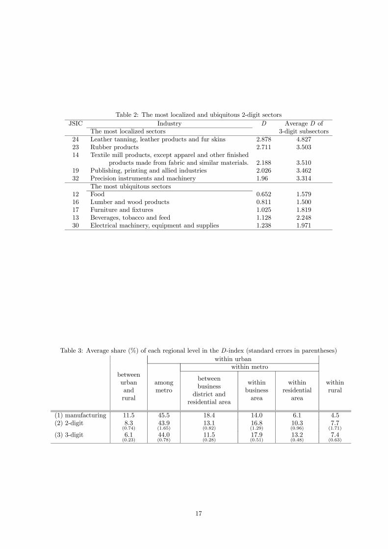
Table 2: The most localized and ubiquitous 2-digit sectorsJSIC Industry D Average D of

The most localized sectors 3-digit subsectors24 Leather tanning, leather products and fur skins 2.878 4.82723 Rubber products 2.711 3.50314 Textile mill products, except apparel and other finished

products made from fabric and similar materials. 2.188 3.51019 Publishing, printing and allied industries 2.026 3.46232 Precision instruments and machinery 1.96 3.314

The most ubiquitous sectors12 Food 0.652 1.57916 Lumber and wood products 0.811 1.50017 Furniture and fixtures 1.025 1.81913 Beverages, tobacco and feed 1.128 2.24830 Electrical machinery, equipment and supplies 1.238 1.971

Table 3: Average share (%) of each regional level in the D-index (standard errors in parentheses)within urban

within metrobetweenurbanandrural

amongmetro

betweenbusinessdistrict and

residential area

withinbusinessarea

withinresidentialarea

withinrural

(1) manufacturing 11.5 45.5 18.4 14.0 6.1 4.5(2) 2-digit 8.3

(0.74)43.9(1.65)

13.1(0.82)

16.8(1.29)

10.3(0.96)

7.7(1.71)

(3) 3-digit 6.1(0.23)

44.0(0.78)

11.5(0.28)

17.9(0.51)

13.2(0.48)

7.4(0.63)

17

with respect to the urban-rural partition can be written as

D(bpi|p0) = D(bqi|q0) + {bqi,urbanD(bpi|urban|p0|urban) + bqi,ruralD(bpi|rural|p0|rural)} (36)

where bqi = (bqi,urban, bqi,rural) now denotes the observed urban-rural distribution of industry i, and wherebpi|urban and bpi|rural denote the observed conditional distributions of industry i across the counties inthe urban and rural areas, respectively. This can be extended to a second level of decomposition by

considering the metro-area partition defining the urban area. If these metro areas are enumerated as

m = 1, ..,M , then the term, D(bpi|urban|p0|urban), can be decomposed further as follows:D(bpi|urban|p0|urban) = D(bqi|metro|q0|metro) + MX

m=1

bqimD(bpi|m|p0|m) (37)

where bqi|metro = (bqim : m = 1, ..,M) now denotes the observed distribution of industry i across metro

areas, and bpi|m denotes the observed conditional distribution of i across the counties in metro area m.

To evaluated this decomposition, it is convenient to focus on all manufacturing (1-digit level) where

i denotes the single “aggregate” manufacturing industry. Here the “between urban and rural” share of

the D-index is given in terms of (36) and (37) by

D(bqi|q0)D(bpi|p0) × 100 = 11.5 (38)

and similarly, the “within rural” share is given by

bqi,ruralD(bpi|rural|p0|rural)D(bpi|p0) × 100 = 4.5. (39)

The “within urban” share then consists of the remainder:

bqi,urbanD(bpi|urban|p0|urban)D(bpi|p0) × 100 = 100− (11.5 + 4.5) = 84. (40)

This latter share can be further decomposed as in (37). Here the “among metro” share is given by

bqi,urbanD(bqi|metro|q0|metro)D(bpi|p0) × 100 = 45.5 (41)

and the “within metro” share is given by

bqi,urban MXm=1

bqimD(bpi|m|po|m)D(bpi|p0) × 100 = 84− 45.5 = 38.5. (42)

18

Lower (i.e., finer) level decompositions can be obtained in a similar manner.

At all industry aggregation levels, localization “among metro areas” explains nearly half of the D-

value. Notice however that localization “within metro areas” is also fairly large. In addition, notice that

as industry classification becomes finer, the average shares of concentration “within business areas” as well

as “within residential areas” increase, while the average shares “between business areas and residential

areas” decrease. Since the average D-value increases as classification becomes finer (1.1, 1.9, and 2.9,

respectively, for 1-digit, 2-digit, and 3- digit industries), the decrease in average shares “between business

areas and residential areas” shows that this increased localization is not simply attributable to greater

concentration in business areas. In fact, the increased shares for both “within business areas” and “within

residential areas” show that this distinction itself is less clear for finer classifications of industries.

Now, let us look across 3-digit industries at the relationship between the D-value and its regional

components. Table 4 shows the correlation42 between the log of the D-index and its corresponding shares

for various decomposition levels. Observe that the share of concentration “among metro areas” and that

“within business areas” are both positively correlated with D. This reflects the fact that more localized

industries are found not only in a fewer number of metro areas, but also in a fewer number of counties

within the corresponding business areas.

This localization pattern can also be seen in relationship between the population size of a metro

area and the degree of localization of industries found in that metro area. Figure 3 plots the highest,

median, and lowest D-values for all industries located in each metro area against the population size of

that metro area.43 The correlations of these three values with the population size of a metro area are

0.52, 0.20 and −0.31, respectively. The plot roughly suggests that a larger metro area attracts both more

localized and ubiquitous industries, while smaller metro areas tend to contain mostly ubiquitous industries.

This, in turn, is roughly consistent with Christaller’s (1933) well-known Hierarchy Principle of industrial

locations, namely that industries present in a given metro area are also present in all the larger metro

areas.44

4.3 Changes in the industrial localization over time

In this section, we look at changes in the degree of localization of 3-digit manufacturing industries in

Japan between 1981 and 1999. Since this industrial classification has been disaggregated for most sectors

between these two periods, we have attempted to reconcile the two classifications by aggregating the

1999 classification to that of 1981, resulting in 148 industries. The D-index of manufacturing as a whole

decreased by more than 10% during this period. Among individual industries, D-values decreased for

63% of these industries (refer to Figure 4).45

19

Table 4: Correlation between D and the share of D at each region level (3-digit)

urban-rural among metro between business areaand residential area

withinbusiness area

withinresidential area

withinrural area

-0.46 0.45 -0.25 0.34 -0.43 -0.22

Figure 3: Population size and industrial structure of metro areas

Note: Markers , and indicate respectively the highest, median and lowestD-values of industrieslocated in each metro area.

104 105 106 107 108

8

7

6

5

4

3

2

1

0

D

Population size

Figure 4: Change in the D-value between 1981 and 1999

5

4

3

2

1

0

-1

-2

-3

-40 2 4 6 8 10

D in 1981

Cha

nge

inD

(diff

eren

ce)

20

As depicted in Figure 5, an increase in D appears to be associated with an increase in the share of

concentration among metro areas (with correlation of 0.39, significant at 1% level). No other changes in

shares were found to be significantly related to changes in D. This result suggests that changes in the

localization of industries take place mainly at the level of metro areas.

4.4 Comparison with Ellison and Glaeser’s G

Finally, in this section, we compare our D-index with the widely used “G” index of localization proposed

by Ellison and Glaeser (1997). In particular if we now let Mir denote the employment level of industry

i in region r (rather than the number of establishments), and let the total employment level of industry

i be denoted by Mi =PrMir , then the share of region r in the employment of industry i is given by

sir = Mir/Mi. In this case, an alternative reference measure is given by the share of total industrial

employment in each region r, i.e., by xr =PjMjr/

PjMj . If sum-of-squared errors is adopted as the

relevant measure of deviation, then the G-index of localization for industry i is given by:

G(si, x) ≡ Σr(sir − xr)2 (43)

where si = (sir : r ∈ R) and x = (xr : r ∈ R).

It should also be noted here that the popular “γ” index proposed by Ellison and Glaeser (1997) is based

on G. More precisely, γ extends G to include establishment-size effects within each industry. Unfortu-

nately, since establishment-size data is not publicly available in Japan (as well as in many other countries),

we can only make empirical comparisons of D with G, and not γ. However, it should be emphasized that

the basic measure of localization in γ is still given by G, and in fact that there is often little practical

difference between the two. To see this, let S =Pr x

2r denote the regional “employment-diversity” index,

and for each industry i with establishment sizes (Mij : j = 1, ..,mi), let Hi =Pmi

j=1(Mij/Mi)2 denote

the “establishment-size-diversity” index for i. Then the γ-index for industry i is defined by46

γi =Gi − (1− S)Hi(1− S)(1−Hi)

= aiGi − bi (44)

where ai = 1/[(1 − S)(1 −Hi)] , bi = Hi/(1 −Hi) , and where Gi denotes the G-index for industry i.

Hence for any fixed S and Hi, this index is seen to be a simple positive affine transformation of Gi. In

particular this implies that if each industry were to have the same number of establishments, all of equal

size within each industry, then this affine function would be the same for all industries. Under these

conditions, the orderings of γi and Gi values would be identical. More generally, if each industry has

many establishments, all of which are roughly comparable in size, then values of Hi are not only similar,

they must all be very close to zero.47 Hence one can expect that ai ≈ 1/(1−S) and bi ¿ Gi/(1− S), so

21

that again the orderings of γi and Gi will be almost the same.48

Figure 6 depicts the relationship between values of the G and our D for all 3-digit manufacturing

industries in 1999. It is not surprising that these indices exhibit substantial disagreement on a case-by-

case basis, given the fundamental difference between their implicit notions of “localization.” While they

do have a fairly high positive correlation [0.5 between log(G) and D], it should be emphasized that this

does not imply similar behavior of the two indices (see Appendix A for details).

One reason for this positive correlation in the Japanese case may be that more localized industries

(in terms of D) tend to have smaller employment shares, as seen in Figure 7.49 Also recall (Section 2.2,

see also Appendix A) that for a given regional employment distribution within an industry, smaller total

employment levels yield higher degrees of localization according to the G-index. It is this relation between

employment shares and degrees of localization for the G-index that appears to be creating this positive

correlation. However, while the D-value is independent of the size variation of industries, the ordering

of G-values for industries can change drastically as relative sizes change (see Appendix A for further

details).

Finally it should be emphasized that the above comparison of the G-index with our D-index is based

directly on Ellison and Glaeser’s definition of G. While this is the simplest and most obvious comparison

to make, it can be argued that such comparisons implicitly involve a number of different dimensions:

(1) What “industry-size distributions” are used?

(2) What regional “reference distributions” are used?

(3) What “functional forms” are used to compare these distributions?

Here it turns out that D and G differ in all three dimensions: not only are their functional forms

different, but also their industry-size distributions ( i-establishment shares, bpir, forD versus i-employmentshares, sir, for G), and their regional reference distributions (economic area shares, p0r, for D versus total

employment shares, xr, for G). One referee described this as comparing “apples with oranges.” So why not

construct a range of “intermediate” indices by modifying either D or G (or both) to yield pairs of indices

that are more comparable? For example, to achieve greater comparability with respect to dimensions (1)

and (2) above, one might modify G to involve comparisons of bpir with p0r [i.e., G0 = Pr(bpir − p0r)2],

or modify D to involve comparisons of sir and xr [i.e., D0 =Pr sir ln(sir/xr)]. Such modifications

are certainly of interest, and may ultimately help to clarify the relationships between these different

dimensions. But for our present purposes, we choose not to attempt such an ambitious program.

22

Figure 5: Change in D and its inter-metro area share

2.5

2

1.5

1

0.5

0 -4 -2 0 2 4Change in D (difference)

Cha

nge

in in

ter-

met

ro sh

are

(rat

io)

Figure 6: Relationship between D and Ellison and Glaeser’s G

10

1

10-1

10-2

10-3

10-40 2 4 6 8 10

Log

(G)

D

23

5 Concluding remarks

In this paper we have developed aD-index of industrial localization based on Kullback-Leibler divergence.

This measure not only has a natural interpretation in terms of relative likelihoods, but also has a simple

asymptotic normal distribution theory that allows the construction of both confidence bounds on the

degree of localization for individual industries and tests of the relative degree of localization between

industries. As shown in Section 4.3, this testing procedure can also be applied to detect temporal changes

in the degree of localization for individual industries.

Given these positive features of the D-index, it is important to emphasize that it does have certain

limitations. First, with respect to the random sampling framework used to motivate this index, it should

be clear that actual industrial location behavior is in fact a dynamical process in which the location of any

new establishment tends to depend quite heavily on the locations of existing ones.50 Moreover, given the

prevalence of multi-plant firms, our independence assumption for plant locations is at best a convenient

fiction. In particular, this implies that our proofs of asymptotic normality for D [see eqs.(4, 5)] may not

hold. However, it should be emphasized that asymptotic normality itself is much more robust, and hence

that our hypothesis tests may still be reasonable as long as dependencies between establishment are not

“too strong.”51

Finally, since no explicit geographic relationships among regional units are embodied in D, this index

can at best give only a limited indication of the actual spatial extent of localization (as illustrated in

Section 4.2 above). For example, concentrations of establishments in contiguous counties may yield

the same D-values as concentrations in widely separated counties. Hence, while the former suggests the

possibility of a larger geographic concentration of establishments, this can only be captured by appropriate

spatial decompositions ofD. Such issues are more appropriately addressed by models at the establishment

level, where modifiable areal unit problems do not arise [as for example in Duranton and Overman (2005)

and Marcon and Puech (2003)].

24

Appendix.

A Choice of reference distribution

In essence, ourD index amounts to a measure of deviation from a given reference distribution representing

an implicit null hypothesis about industrial location patterns. However, there are other choices for

both the reference distribution used and the measure of deviation from that distribution. Hence it is

appropriate in this appendix to compare our choice with one of the most popular measures of this type,

the G-index of Ellison and Glaeser (1997), introduced in Section 4.4, where an alternative reference

measure is given by the share of each region in all industrial employment.52

An obvious motivation for measuring localization in relative terms is to remove the effect of regional

population size. For if there is significant size variation among regions, then it is natural to expect to

find larger employment levels for industries in larger regions. But unless all the regions have identical

shares of each industry, this normalization can distort the index in certain systematic ways. For under

this type of normalization, those industries with a larger share of total national employment will appear

to be more ubiquitous. This is mainly due to the fact that the employment share distribution, sir, for

large industries i will then be very similar to the total regional employment shares, xr. At the other

extreme, small industries are likely to appear to be very localized — even if their employment distribution

is in fact quite uniform across regions. These observations are well illustrated by the following two simple

examples.

Regional diversity effect

Difference in industrial diversity among regions can lead to ambiguities in the interpretation of the

G-index.53 In particular, while large metro areas, like Tokyo, tend to have greater employment in each

industry than do small metro areas, the employment shares of individual industries tend to be smaller in

large metro areas simply because of the greater industrial diversity in those areas. Hence, indices based

on relative concentration, such as G, tend to undervalue the localization of industries in large metro

areas, even when their absolute levels of employment are quite high.

To see this, consider the following core-periphery system of two regions, where the core region has

both manufacturing and agriculture, while the periphery has only agriculture (as illustrated in Figure

8). Here, manufacturing is a “localized” sector (of size 1− q, where 0 < q < 1) completely concentrated

in region B, while agricultural is a “ubiquitous” sector (of size q) uniformly distributed over the two

regions. But under index G we have Glocalized = 12(1− q)2 and Gubiquitous =

12q2, where the subscripts

denote the “localized” manufacturing sector and “ubiquitous” agricultural sector respectively. Hence

25

Figure 7: Relationship between D and employment share of an industry

1

10-1

10-2

10-3

10-4

10-5

10-6

10-70 2 4 6 8 10

D

Log

(em

ploy

men

t sha

re)

Figure 8: Core-periphery regional system

Region A

manufacturing

agriculture→→

1 - q

q/2 q/2Region B

26

Gubiquitous R Glocalized if q Q 1/2, and it follows that when the “ubiquitous” sector is relatively small, the

G-index always evaluates this sector as more localized than the “localized” sector. Thus, by completely

ignoring the spatial aspect of the employment distribution, and by defining “localization” solely in terms

of the underlying population (or employment) distribution, a spatially concentrated sector may appear

to be more ubiquitous than a spatially dispersed sector.

It should also be noted that this same example can be applied to the γ-index of Ellison and Glaeser.

For if we assume (not unreasonably) that there are a large number of small “ubiquitous” farms and a

large number of small “clustered” manufacturing establishments in Region B, then (as argued in Section

4.4 above) the ordering of γ and G should be the same in this case.

Note finally for this example that if the reference distribution in our D-index is replaced by regional

employment shares [i.e., if D(pi|p0) is replaced by D(si|x)] then it can be easily verified that Dlocalized = 0

and Dubiquitous = log(2) for any choice of q. So the same problem arises, and it is clear in this case that

it is the choice of reference distributions (and not the measure of deviation) that is creating this anomaly.

Industry size effect

Next, we examine the effect of industry size on alternative indices of localization. Again consider an

economy with two regions and two industries. Suppose that each industry is relatively concentrated in a

different region, and that the interregional distribution of employment is symmetric between the two, i.e.,

that each region has the same share of total employment in its specializing industry. Specifically, let the

total employment for industry 1 [resp., 2] be given by q [resp., 1− q], where 0 ≤ q ≤ 1. In addition, let

the share of region A [resp., B ] in the employment for industry 1 [resp. 2] be given by p, where 0 ≤ p ≤ 1

(as summarized in Table 5 below). Note that the regional shares of employment for the two industries

are symmetric (i.e., region A has a share, p, of industry 1 and region B has the same share, p, of industry

2).

Table 5: Employment concentration of industries with different sizeindustry 1 industry 2

region A pq (1− p)(1− q)region B (1− p)q p(1− q)

The values of G for industries 1 and 2 are given respectively by G1 = 2(2p − 1)2(1 − q)2 and

G2 = 2(2p − 1)2q2. Here it can readily be verified that G1 > G2 if p 6= 1/2 and q < 1/2. Hence,

unless employment for each industry is evenly distributed across regions, the smaller industry is always

evaluated as more concentrated. As discussed above, this example gives a dramatic illustration in which

the total employment distribution is always “closer” to that of the larger industry, thus making that

industry appear more ubiquitous.54 Note finally that the argument for γ made in the last example again

27

shows that if both industries have a large number of small firms, then the ordering of γ and G should be

the same, so that γ tends to exhibit the same problem.

More generally it should be emphasized that size variations among industries may be due to fundamen-

tal structural differences between these industries, such as production technology or market structures.

Hence it is our view that indices of industrial localization should not depend on such industry-specific

characteristics. In particular, ourD-index is independent of sector size (and in the example above we have

D1 = D2 for any p and q). However, if the reference distribution for D is set to the distribution of ag-

gregate industry [i.e., if D(pi|p0) is replaced by D(si|x)], then it can be verified that D1 R D2 ⇔ p R 1/2

when q < 1/2. Hence relative specialization influences the degree of localization. More specifically, even

if interregional distribution is symmetric for industries i and j (as in this example), if the region where

industry i is localized is relatively more specialized in i than the other region is in j, then industry i is

evaluated to be more localized than j. Hence for the D-index, this choice of reference distributions can

in some cases create a confusion between the degree of specialization for industries and their degree of

geographic concentration.

B Proof of Theorem 1

From the derivation in Section 3.1, we know that for large ni the D-index, D(bpi|p0), is approximatelynormally distributed with mean, D(pi|p0), and variance, σ2(bpi|p0)/ni (eq., (29)) if bpir > 0 for all i andr. Thus, we are left to show that each component r of bpi with bpir = 0 can simply be dropped from the

estimation of variance (29).

In the present case this is less of a problem since we are only considering a one-dimensional function

of bpi. Here it suffices to establish a limiting form for var[D(bpi|p0)] when one or more components of bpiapproaches zero. To do so, let us simplify the notation to

g(x) = ∇D(x|p0) (45)

and consider the limit of the quadratic form, ∇D (x|p0)0Σ(x)∇D (x|p0) =Pr

Ps g(xr)Σrs(x)g(xs) as

xr → 0. First observe from (21) and (25) that if for each r = 1, .., R− 1 we now let

θr(x) = ln³1−

PR−1s=1 xs

´+ ln

Ãp0r

1−PR−1s=1 p0s

!(46)

28

then for all distinct regional pairs, rs,

g(xr)Σrs(x)g(xs) = [ln(xr)− θr(x)] (−xrxs) [ln(xs)− θs(x)]

= − [xr ln(xr)− xrθr(x)] [xs ln(xs)− xsθs(x)] . (47)

But since limxr→0 xr ln(xr) = 0, and since

limxr→0

θr(x) = ln³1−

Ps6=r xs

´+ ln

Ãp0r

1−PR−1s=1 p0s

!(48)

is bounded, it follows from (45) that

limxr→0

g(xr)Σrs(x)g(xs) = 0 (49)

Next consider the rth diagonal term

g(xr)2Σrr(x) = [ln(xr)− θr(x)]

2xr(1− xr)

= xr [ln(xr)]2 − 2 [xr ln(xr)] θr(x) + xrθr(x)2 − [xr ln(xr)− xrθr(x)]2 (50)

and observe from the arguments above that the last three terms go to zero as xr → 0, so that

limxr→0

g(xr)2Σrr(x) = lim

xr→0xr [ln(xr)]

2 . (51)

To establish the limit of the right hand side of (51), let f(xr) = [ln(xr)]2 and h(xr) = 1/xr so that

xr [ln(xr)]2 =

f(xr)

h(xr). (52)

Observe in addition thatf 0(xr)

h0(xr)=2 [ln(xr)] /xr

−x−2r= −2xr ln(xr) (53)

implies limxr→0 [f0(xr)/h

0(xr)] = 0, and moreover that limxr→0 f(xr) = ∞ = limxr→0 h(xr). By

L’Hospitals Rule55 it then follows that limxr→0 [f(xr)/h(xr)] = 0 and hence that

limxr→0

g(xr)2Σrr(x) = 0 (54)

Thus each component r of bpi with bpir = 0 can simply be dropped from the estimation of variance in

(29).56 If we now let bp+i = {r=1, .., R− 1: bpir > 0}, then we obtain Theorem 1¥

29

C Inter-industry comparison of localization degrees

Figure 9 indicates the industries (vertical axis) whose D-values are not significantly different (at 1% level)

from that of a given industry (horizontal axis), based on 1999 data. The regional units are counties in

Diagram (a) and prefectures in Diagram (b).57 Industries are ranked in terms of their D-values (i.e., the

industry with the largest D is rank 1). Notice that at both of these regional levels, most industries are

quite distinguishable in terms of their degree of localization. This is mainly due to the large sample sizes

(industry sizes), which yield sharp confidence bounds on individual D-values.

30

Figure 9: Test of the difference in localization degrees between industries

Rank of industries in terms of D

(a) County level

0 20 40 60 80 100 120 140 160

160

140

120

100

80

60

40

20

0

Indu

strie

s who

seD

-val

ue is

not

sign

ifica

ntly

diff

eren

t at 1

% le

vel

Rank of industries in terms of D

(b) Prefecture level

160

140

120

100

80

60

40

20

0

Indu

strie

s who

seD

-val

ue is

not

sign

ifica

ntly

diff

eren

t at 1

% le

vel

0 20 40 60 80 100 120 140 160

31

ReferenceBartle, Robert G., The Elements of Real Analysis, Second Edition (New York: John Wiley & Sons, Inc,

1976).

Bourguignon, Francois, “Decomposable income inequality measures,” Econometrica 47 (1979), 901-920.

Brülhart, Marius, and Rolf Traeger, “An account of geographic concentration patterns in Europe,” forth-

coming in Regional Science and Urban Economics (2005).

Christaller, Walter., Die Zentralen Orte in Süddeutschland (Gustav Fischer, 1933), English translation

by Carlisle W. Baskin, Central Places in Southern Germany (Englewood Cliffs, NJ: Prentice Hall, 1966).

Cover, Thomas M., and Joy A. Thomas, Elements of information theory (New York: John Wiley & Sons,

Inc., 1991).

Dembo, Amir, and Ofer Zeitouni, Large Deviation Techniques (Boston: Jones and Bartlett Publishers,

1993).

Doukhan, Paul, Mixing: Properties and Examples (New York: Springer-Verlag, 1994).

Duranton, Gilles, and Henry G. Overman, “Testing for localization using micro-geographic data,” forth-

coming in Review of Economic Studies (2005).

––—, and Diego Puga, “Micro-foundation of urban agglomeration economies,” in J. Vernon Henderson

and Jacques-François Thisse (eds.), Handbook of Urban and Regional Economics, vol.4 (Amsterdam:

North-Holland, 2004), 2063-2117.

Ellison, Glenn, and Edward L. Glaeser, “Geographic concentration in U.S. manufacturing industries: a

dartboard approach,” Journal of Political Economy 105 (1997), 889-927.

Gibbs, Allison L., and Francis Edward Su, “On Choosing and Bounding Probability Metrics,” Interna-

tional Statistical Review 70, 419-435 (2002).

Japan Statistics Bureau, Establishment and Enterprise Census (1981,1999).

––—, Population Census (2000).

Krugman, Paul, Geography and Trade (Cambridge, MA: MIT Press, 1991), Ch.2.

Kullback, Solomon, Information Theory and Statistics (New York: John Wiley & Sons, Inc., 1959).

32

––—, and Richard A. Leibler, “On information and sufficiency,” Annals of Mathematics and Statistics

22 (1951) 79-86.

Kanemoto, Yoshitsugu, and Kazuyuki Tokuoka, “The proposal for the standard definition of the metro

area in Japan,” Journal of Applied Regional Science 7 (2002), 1-15.

Marcon, Eric, and Florence Puech, “Evaluating the geographic concentration of industries using distance-

based methods,” Journal of Economic Geography 3 (2003), 409-428.

Mori, Tomoya, Nishikimi, Koji, and Tony E. Smith, “Some empirical regularities in spatial economies: a

relationship between industrial location and city size,” Discussion paper No.551, Institute of Economic

Research, Kyoto University (2002).

Ripley, Brian D., “Modelling spatial patterns’, Journal of the Royal Statistical Society B, 39 (1977),

172-192.

Rao, C. Radhakrishna, Linear Statistical Inference and Its Applications, Second Edition (New York: John

Wiley & Sons, Inc., 1973).

Rosentahl, Stuart S., and William C. Strange, “Evidence on the Nature and sources of agglomeration

economies,” in J. Vernon Henderson and Jacques-François Thisse (eds.), Handbook of Urban and Regional

Economics, vol.4 (Amsterdam: North-Holland, 2004), 2119-2171.

Salas, Rafael, “Multilevel interterritorial convergence and additive multidimensional inequality decom-

position,” Social Choice and Welfare 19 (2002), 207-218.

Shorrocks, Anthony F., “The class of additively decomposable inequality measures,” Econometrica 48

(1980), 613-625.

––—, “Inequality decomposition by factor components,” Econometrica 50 (1982), 193-211.

––—, “Inequality decomposition by population subgroups,” Econometrica 52 (1984), 1369-1385.

Smith, Tony E., “A Central Limit Theorem for Spatial Samples”, Geographical Analysis 12 (1980), 299-

324.

Statistical Information for Consulting Analysis, Tokei de miru Shi-Ku-Cho-Son no Sugata, in Japanese

(1998).

Theil, Henri, Economics and Information Theory (Amsterdam: North-Holland, 1967).

33

Thistle, Paul D., “Large sample properties of two inequality indices,” Econometrica 58 (1990), 725—728.

Wilks, Samuel Stanley, Mathematical Statistics (New York: John Wiley & Sons, Inc., 1962).

34

Notes

1See, Rosenthal and Strange (2004) for a survey of this literature.

2A notable exception is the K-density approach of Duranton and Overman (2005) and Marcon and

Puech (2003) [based on Ripley (1977)]. But while this method provides a powerful framework for sta-

tistical analyses of industrial localization (and in particular is free of the border biases arising from

internal regional subdivisions), it requires location data at the level of individual establishments within

each industry, and such data is often not available.

3It should also be noted that unlike other existing indices, our index requires only regional-level data

that is widely available. In particular, it does not require information about either the locations or sizes

of specific establishments [as for example in Duranton and Overman (2005), Marcon and Puech (2003),

Ellison and Glaeser (1997)]. Hence this index should provide a handy tool for a wide range of researchers

interested in studying spatial localization.

4As shown in Section 4.3, it is also useful for testing inter-temporal changes in the degree of localization

within a given industry.

5A notable exception is the measure of “topographic concentration” by Brülhart and traeger (2005),

discussed in footnote 8 below.

6The implications of alternative choices of reference distributions are discussed in more detail in Section

4.4 and Appendix A.

7The related literature for such decompositions is found in footnote 17.

8At this point it should be noted that an approach similar to the present one has been developed

independently by Brülhart and Traeger (2005) for the analysis of inter-temporal changes in spatial con-

centration. Following the works of Bourguignon (1979) and Shorrocks (1980, 1982, 1984) these authors

propose a class of “generalized entropy” measures (GE) based on their desirable decomposability prop-

erties. Among these is the present D-index [designated as GE(1)], where the appropriate reference

distribution is implicitly taken to be defined by the choice of units for analysis. Our hypothesis of com-

plete spatial dispersion corresponds to the choice of areal units of analysis, designated by Brülhart and

Traeger as topographic concentration. However, in the present approach we take this reference distri-

bution to represent an explicit null hypothesis for testing differences in spatial concentration between

industries. Under the assumption of independent random sampling (discussed in Section 2.1 below), each

null hypothesis leads to an explicit asymptotic normal distribution for differences in spatial concentra-

35

tion (as developed in Section 3.1 below). In contrast, the above authors adopt a nonparametric “block

bootstrap” testing procedure for identifying significant changes in spatial concentration over time. While

this procedure does allow for possible spatial dependencies over time, it is not specific to any particular

index of spatial concentration.

9It is of interest to note, however, that this approximation at the establishment level may be more

reasonable than at the level of individual workers. In particular, one could equally well calculate the

degree of localization for distributions of employment rather than establishments. But since the locations

of workers are tied to those of the establishments in which they are employed, statistical independence

at the worker level seems even less plausible.

It should also be noted that patterns of establishment location may differ depending on their em-

ployment size [as reported by Duranton and Overman (2005) for the case of the UK]. However, the

application of our D-index (introduced below) to Japanese manufacturing industries suggests that the

degrees of localization based on employment-size data and establishment data are in close agreement

(Spearman’s rank correlation is greater than 0.9). That is, the establishment size variation among indus-

tries as well as the size-dependence of locational patterns appears to have only minor influence on the

degree of localization measured by our index.

This result still leaves open the possiblity that correlation of location behavior occurs at more ag-

gregated level, i.e., the location of multiple establishments may be correlated to some extent given the

prevalence of multi-unit firms. However, the present limitations of data availability make it difficult to

address these questions.

10A recent survey of such measures can be found in Gibbs and Su (2002).

11Kullback-Leibler divergence can also be motivated from an information-theoretic viewpoint [e.g.,

Cover and Thomas (1991)].

12While the reference distribution, p0r, is always positive for all r for our purposes, the i-establishment

distributions, pir, need not be positive. Hence the definition of D(pi|p0) implicitly includes the convention

that 0 ln(0) = 0.

13The function D(·|p0) is strictly convex on the interior of the probability simplex in RR−1, and hence

achieves its maximum values at the vertices of this simplex. For the vertex with pir = 1, the local

maximum value of D is easily seen to be − ln(p0r) > 0, so that the global maximum is achieved when

p0r achieves its minimum value over r = 1, .., R. In other words, D is as large as possible when all

establishments are concentrated in the region of smallest (economic) size.

36

14See, e.g., Sanov’s Theorem in Dembo and Zeitouni (1993).

15It is well known that, the statistic, -2lnλ, is asymptotically chi-square distributed with R− 1 degrees

of freedom, and hence, provides a well-defined statistical test of the null hypothesis, pi = p0.

16For the Japanese case in particular, there is a strong negative correlation (Spearman’s rank correlation

of -.66) between the number of establishments and the D-index for 3-digit manufacturing industries. So

more ubiquitous industries do indeed tend to have larger numbers of establishments.

17Studies of the decomposability properties of entropy measures in information theory date back to the

seminal work of Kullback (1959) [as summarized in Cover and Thomas (1991)], and were first introduced

into economics by Theil (1967). It was later shown by Bourguignon (1979) and Shorrocks (1980, 1982,

1984) that these decomposability properties essentially characterize entropy (i.e., are uniquely exhibited

by a somewhat more general class of entropies ). A systematic survey of this work can be found in

Brülhart and Traeger (2005). See also Salas (2002) for a recent survey.

18A notable exception here is the work of Brülhart and Traeger (footnote 8 above) who have indepen-

dently used the same decomposition techniques to compare industrial concentrations both within and

between 16 countries of Western Europe.

19It should be noted that Ellison and Glaeser (1997) do calculate the variance of G under the null

hypothesis of no regional-endowment effects or spillover effects (γna = 0 = γs), and make an implicit

appeal to asymptotic normality of G in order to test this null hypothesis. However, no attempt is made

to derive general confidence intervals for either E(G) or E(γ). With respect to divergence indices, it

should also be noted that Brülhart and Traeger (2005) apply bootstrap methods to estimate confidence

intervals for an index identical to our D.

20For convenience we use the same regional notation, r, for the numerical region index in this section.

21This implies in particular that for all r, s = 1, .., R−1, var(Nir) = nipir(1−pir), and cov(Nir,Nis) =

−nipirpis. In addition, the variance of NiR and the covariance between NiR and Nir for r = 1, 2, ...R− 1

are given by

var(NiR) = ni

µ1−

XR−1

s=1pis

¶XR−1

s=1pis

= niz0[diag(pi)− pip0i]z,

37

cov(NiR, Nir) = −nipirµ1−

XR−1

s=1pis

¶= −ni[diag(pi)− pip0i]z,

where z is a (R− 1)-vector with all elements equal to one.

22If one or more components of pi are zero, then special care must be taken in defining the appropriate

region of differentiation (to be explained below).

23This asymptotic normality result is in fact an instance of more general results obtained by Thistle

(1990) (i.e., the limiting case of his Theorem 3 as β → 0).

24A number of examples of this type were simulated, and all produced similar results.

25For the Japanese manufacturing to which we apply our D-index in Section 4, there is no industry i

for which the null hypothesis pi = p0 cannot be rejected under the likelihood-ratio test (refer to footnote

15).

26For the case of Japan, the average and median number of establishments for 3-digit industries are

4692 and 1941, respectively. The industry at the 10 percentile point has 105 establishments. It is to be

noted, however, that those industries with small numbers of establishments are rather specialized. The

smallest 10% (17 industries) include the tobacco industry, eight arms related industries, and two heavily

natural-resource oriented industries (coke and briquettes manufacturing). Thus, most market oriented

private industries have fairly large numbers of establishments at the 3-digit level.

27To estimate the true size of this test, we set pi = pj = (.1, .4, .2, .3), and sampled 1000 values of bothbpi and bpj , from this common distribution [yielding 1000 samples of the test statistic, D(bpi|p0)−D(bpj |p0)].For the rejection region of size α = .05 based on normal theory, our estimate bα was simply the fraction oftimes this test statistic fell in the rejection region, i.e., the fraction of time that the true null hypothesis,

pi = pj , was rejected.

28The establishments and employment data used in this section are classified according to the Japanese

Standard Industry Classification (JSIC) taken from the Establishment and Enterprise Census of Japan

[Japan Statistics Bureau (1981, 1999)]. In addition to 3-digit classification, we also consider 2-digit

classification later in this section.

29Economic area is obtained by subtracting the forest, undeveloped area, lakes and marshes from the

total area of a county [Data source: Statistical Information Institute for Consulting and Analysis (1998)].

38

The total economic area is 120,205km2, equivalent to 31.8% of total area in Japan. The size of economic

area in a county varies from 0.47km2 to 720.38km2 with average 37.21km2.

As pointed out by one of the referees, economic area is to some extent an endogenous variable. For

instance, forest may be converted to industrial area. But 70% of Japanese land was covered by forest in

1998, and for our purposes it seems reasonable to assume that the forest continues to cover large portion

of Japanese land at the present time.

It should also be noted that several alternative definitions of economic area might be appropriate,

depending on the objectives of a given study. But the validity of our D-index itself is independent of any

particular definition of economic area.

30County here is equivalent to shi-ku-cho-son in the Japanese Census. County boundaries are as of

October 1, 2001. The number of counties in Japan is 3363.

31This is most evident in Figure 9 of Appendix C below, where it is seen that all but the smallest

differences in D-value rankings are significant at the 1% level.

32Refer to Section 2.3 and footnote 16.

33The industries that are excluded from Table 1 but have higher D-values than those listed are all

the eight arms-related industries (JSIC331-339, D = 6.52 ∼ 8.59), fur skin manufacturing (JSIC248,

D = 5.89), Coke (JSIC213, D = 4.82), Briquette and briquette balls manufacturing (JSIC214, D = 4.66),

Mechanical leather products, excluding gloves and mittens (JSIC242, D = 4.56).

34See Appendix C for more detail on the comparison of D-values among industries.

35See, e.g., Duranton and Puga (2004) for a survey of the micro foundations of agglomeration economies.

36However, the ubiquity of cement-related industries may also be partly explained by the ubiquity of

lime in Japan.

37Again, ordnance and accessories (JSIC33) is excluded in the list since it has only 29 establishments.

The D-value for this industry is 5.43.

38The size of the 99% confidence band for each industry is smaller than 0.001.

39Derivation of metro areas is based on Urban Employment Area (UEA) developed by Kanemoto

and Tokuoka (2002) which aggregates counties based on commuting patterns, and is comparable to

the Core Based Statistical Area (CBSA) of the U.S. While their definition of the UEA requires that

the central county of a metro area should have the so-called densely inhavited district (defined in the

39

Population Census of Japan [Japan Statistics Bureau (2000)] with more than 10,000 population, the

threshold population size in our definition is 5,000. But, the basic result is not affected by the choice of

the threshold.

40It should be noted however that our D-index values for these metro areas are based on 1999 employ-

ment data.

41Business areas were constructed by first ranking counties by their numbers of establishments, and

then choosing the highest ranked counties constituting 70% of all establishments.

42These product-moment correlations are all significant at 1% level.

43Population data are taken from the Population Census of Japan [Japan Statistics Bureau (2000)].

44See Mori, Nishikimi and Smith (2002) for a formal test of this principle.

45All changes in the D-index are significant at 1% level. Note that D-index values are likely to be

postively correlated between time period, so that (as mentioned at the end of section 3.3) this level of

significance may even be conservative.

46See Ellison and Glaeser (1997).

47This is seen most easily when all firms in industry i are of exactly the same size, so that Hi =

mi(1/mi)2 = 1/mi ≈ 0. More generally, simple continuity considerations suggest that this will continue

to hold so long as Mi is very large compared to any single Mij .

48Empirical evidence for this can be found in the Ellison-Glaeser (1997) itself. For example, the

orderings of G and γ for the 15 most localized industries in their Table 4 are identical. Moreover, while

this is less evident for the 15 most ubiquitous industries shown in Table 4, these values of γ are all so

close to zero that their actual ordering can be expected to be unstable.

49The (product-moment) correlation between D and the log of employment share is -0.75.

50This is one of the issues first dealt with by Ellison and Glaeser (1997).

51For example, the case of “within multi-establishment” dependencies can be handled within the current

asymptotic framework so long as there is a bound, m, on the number of establishments within each multi-

establishment firms. For then, by ordering establishments by multi-plant firm, the resulting sequence

can be regarded as m-dependent, so that the estimates bpi = (bpir) are still asymptotically multi-normallydistributed [for a spatial version of this result see, for example, Smith (1980)]. More generally, asymptotic

normality continues to hold as long as dependencies between establishments are not “too strong” [see,

40

for example, Doukhan (1994)].

52Another popular measure is the locational Gini coefficient [e.g., Krugman (1991)] which is basically

the sum of the difference between the cumulative share of industry-specific employment Σv≤rsiv and that

of total employment Σv≤rxv for each region r, where regions are ordered by the ratio, sir/xr.

53In 1999, the most diverse metro area in Japan was Tokyo with positive employment in 157 3-digit

manufacturing industries out of the total 166, while the least diverse was Kamifurano with only 10

industries.

54While this problem with the G-index is most evident when one industry is large relative to total

manufacturing, the same problem persists for finer industrial classifications as well. One way to see this

statistically is to imagine cases in which the employment of each industry is drawn from the same regional

“population distribution,” so that industries differ statistically only in terms of their sample size. Then

the Law of Large Numbers tells us that larger industries (samples) can be expected to resemble the

population distribution more closely than smaller industries (samples).

55For details of L’Hospital’s Rule, see for example Bartle (1976).

56It should be noted that since the limit of θr(x) is well defined and bounded for any subset of x

approaching zero, the above argument is directly extendable to the case of multiple zero components.

57There are 47 prefectures in Japan.

41