A DESIGN FLOOD ESTIMATION PROCEDURE USING DATA GENERATION

AND A DAILY WATER BALANCE MODEL

W. C. Boughton P. I. Hill

Report 97/8

October 1997

ii

Boughton, W.C. (Walter C.) A design flood estimation procedure using data generation and a daily water balance model. Bibliography. ISBN 1 876006 24 2. 1. Flood forecasting – Mathematical models. 2. Hydrologic models. 3. Runoff – Mathematical models. 4. Rain and rainfall – Mathematical models. I. Hill, P.I. (Peter Ian). II. Cooperative Research Centre for Catchment Hydrology. III. Title. (Series: Report (Cooperative Research Centre for Catchment Hydrology); 97/8). 551.4890112 Keywords Floods and Flooding Flood Forecasting Rainfall/Runoff Relationship Modelling (Hydrological) Design Data Catchment Areas Peak Flow Frequency Analysis Water Balance © Cooperative Research Centre for Catchment Hydrology, 1997 ISSN 1039-7361

iii

Preface This report describes work which began early in 1996 as part of CRC Project D1 “Improved loss modelling for design flood estimation and flood forecasting”. It combines the use of site-specific data to calibrate a daily rainfall-runoff model, data generation to provide a long “record” of rainfalls, and peak-to-volume ratios to turn the daily flow volumes into instantaneous maxima. In other words, it uses a holistic approach which avoids the need to compute event losses at all. In a current core research project in the Flood program, the CRC is looking at similar (and alternative) holistic approaches suitable for practitioners for application in rainfall-based design flood estimation. In this context, the work of Boughton and Hill is regarded as an important contribution to the current research. It is published now to encourage further testing and evaluation of the method on other catchments; feedback from users is both solicited and welcome. It is a pleasure to record my appreciation for the continuing involvement of Walter Boughton and Peter Hill in the work of the CRC. Acknowledgment is also given to the Bureau of Meteorology and the (former) Rural Water Corporation for the rainfall and runoff data used in this work. Russell Mein Program Leader

iv

Summary Daily rainfall records form an extensive and valuable data base in most areas of Australia. The use of these records for water supply design is well established, but little use is made of the data in design flood studies. This report describes a new design flood estimation procedure which makes use of the site-specific information in daily rainfall records as an alternative to the generalised rainfall information in Australian Rainfall & Runoff. A daily rainfall generating model uses the relevant statistics from an actual record to generate very long sequences of daily rainfalls. The synthetic sequence becomes input into a daily rainfall-runoff model which generates a corresponding sequence of daily runoff values. Using a relationship between daily volumes of runoff and peak rates of runoff, the annual maxima values of daily runoff are used to estimate the annual maxima distribution of peak rates of runoff. The daily rainfall generating model is a modification of the Srikanthan-McMahon (1985) model. The daily rainfall-runoff model is the AWBM water balance model (Boughton, 1993). Three methods of relating annual `maxima peak flow rates and daily volumes are tested, and a log-log relationship is selected for use. All of the components, i.e. daily rainfall generating model, rainfall-runoff model and peak/volume relationship, have been used before in separate studies. This study brings these components together into a complete design flood estimation procedure. The use of a continuous simulation rainfall-runoff model avoids the treatment of flood runoff as isolated events, and avoids any need to assume values of "losses". The daily rainfall generating model is calibrated against available information on annual maxima daily rainfalls. If only the record of daily rainfalls is available, the model can safely extrapolate to design floods of ARI 500 years. If rainfall extrapolation techniques such as FORGE are available, then design flood estimates to ARIs of 2000 years can be made. If estimates of 24 hour PMP are available, the calibrated model can be used to generate periods of data equal in length to the assumed ARI of the PMP and so enable the distribution of flood peaks up to the PMF to be estimated. The complete design flood estimation procedure is demonstrated using data from the 108 km2 Boggy Creek catchment in Victoria.

v

TABLE OF CONTENTS 1. INTRODUCTION .................................................................................................................... 1 1.1 Purpose of this Study............................................................................................................ 1 1.2 The Need for Design Estimates of Large to Extreme Floods ............................................... 1 1.3 Guide to this Report .............................................................................................................. 2

2. DAILY RAINFALL GENERATION MODEL ........................................................................... 4 2.1 Description of the Study Catchment. .................................................................................... 4 2.2 Description of the Model ....................................................................................................... 6 2.3 Generation within each State................................................................................................ 6 2.4 Calibration of the Model ........................................................................................................ 7 2.5 Errors in Low Values of Generated Rainfall.......................................................................... 9 2.6 Computer Program ............................................................................................................... 9 2.7 Summary ............................................................................................................................ 10

3. DAILY RAINFALL-RUNOFF MODEL .................................................................................. 11 3.1 A Note on Terminology ....................................................................................................... 11 3.2 The DGAWBM Model ......................................................................................................... 12 3.3 Calibration of the DGAWBM............................................................................................... 13 3.4 Generation of Daily Runoff ................................................................................................. 17 3.5 Losses ................................................................................................................................ 17 3.6 Summary ............................................................................................................................ 19

4. RELATING PEAK FLOW RATES TO VOLUME OF RUNOFF ........................................... 20 4.1 Previous Work on Peak/Volume Ratios.............................................................................. 20 4.2 Testing of Methods ............................................................................................................. 20 4.3 Summary ............................................................................................................................ 24

5. RESULTS ............................................................................................................................. 25 5.1 Generation of Daily Rainfalls .............................................................................................. 25 5.2 Generation of Daily Runoff ................................................................................................. 26 5.3 Estimation of Peak Rates of Runoff.................................................................................... 27 5.4 Comparison with Frequency Analysis of Observed Flood Peaks ....................................... 28 5.5 Comparison with other Methods ......................................................................................... 31 5.6 Summary of Results from Boggy Creek ............................................................................. 31

6. CONCLUSIONS ................................................................................................................... 33 6.1 Daily Rainfall Generation Model.......................................................................................... 33 6.2 Daily Water Balance Rainfall - Runoff Model...................................................................... 33 6.3 Peak/Volume Ratio ............................................................................................................. 34 6.4 Application for Design Flood Estimation ............................................................................. 34

7. REFERENCES ..................................................................................................................... 35

APPENDIX A - Calibration results of DGAWBM on Boggy Creek ............................... 35

vi

List of Figures

Figure 1-1 Structure of the Design Flood Estimation Procedure ................................................ 3 Figure 2-1 Map of Boggy Creek Catchment ............................................................................... 5 Figure 2-2 Annual Maxima Daily Rainfalls (catchment average values)- Calibration Data and

Calibrated Model Results.................................................................................................... 8 Figure 3-1 Structure of the DGAWBM...................................................................................... 12 Figure 3-2 Actual versus Calibrated Monthly Runoff from Calibrated DGAWBM (Boggy Creek,

1976-1992) ....................................................................................................................... 16 Figure 4-1 Peak/Volume Ratio from Comparison of Frequency Distributions .......................... 22 Figure 4-2 Peak/Vol Ratio from Fitted Linear Regression ........................................................ 23 Figure 4-3 Peak/Volume Ratio from log-log Linear Regression ............................................... 23 Figure 5-1 Results From Daily Rainfall Generation Model (Average Catchment Rainfall)........ 25 Figure 5-2 Fitted GEV Distribution using LH-Moments for 1976-1992 ..................................... 29 Figure 5-3 Fitted GEV Distribution using LH-Moments for 1967-1992 ..................................... 30 Figure 5-4 Results from Boggy Creek Catchment.................................................................... 32

List of Tables Table 2-1 States of Daily Rainfall................................................................................................ 6 Table 2-2 Transition Probability Matrix for January..................................................................... 6 Table 2-3 Annual Maxima Daily Rainfalls over the Boggy Creek Catchment ............................. 7 Table 2-4 Generated versus Actual Annual Rainfalls ................................................................. 9 Table 3-1 Sample Calculation of Calibration Function.............................................................. 14 Table 3-2 Preliminary Calibration of Stores by DGBASE5 ....................................................... 14 Table 3-3 Parameter Values Calibrated by DGCALIBR and Calibrating Function ................... 15 Table 3-4 Calibrating Function.................................................................................................. 15 Table 3-5 Generated Rainfall and Runoff for A = 13.0 ............................................................. 17 Table 3-6 Generated Rainfall and Unrouted Surface Runoff for A = 13.0 ................................ 18 Table 4-1 Annual Maxima Data from Boggy Creek .................................................................. 21 Table 4-2 Ratio of Actual Peaks and Calculated Daily Flows ................................................... 21 Table 4-3 Peak/Vol Ratios Based on Log-Regression ............................................................. 24 Table 5-1 Results from Daily Runoff Generation Model ........................................................... 26 Table 5-2 Estimates of Peak Rates of Runoff .......................................................................... 27 Table 5-3 Recorded Annual Maxima Flood Peaks (m³/sec) Boggy Creek catchment.............. 28 Table 5-4 Peak Flood Estimates (in m³/sec) from 17 years of Observed Data (1976-1992).... 29 Table 5-5 Peak Flood Estimates (in m³/sec) for 26 years of Observed Data (1967-1992)....... 30 Table 5-6 Comparison of Estimates of Flood Peaks ................................................................ 31

1

1. INTRODUCTION

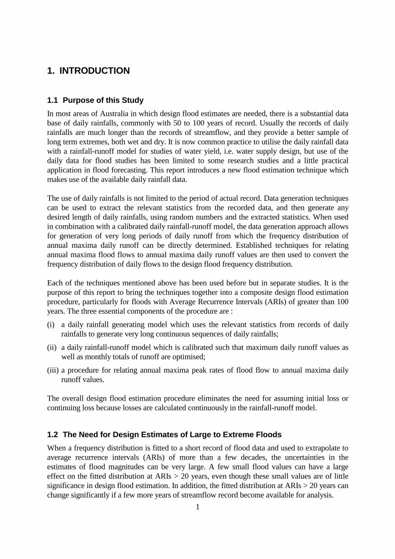
1.1 Purpose of this Study In most areas of Australia in which design flood estimates are needed, there is a substantial data base of daily rainfalls, commonly with 50 to 100 years of record. Usually the records of daily rainfalls are much longer than the records of streamflow, and they provide a better sample of long term extremes, both wet and dry. It is now common practice to utilise the daily rainfall data with a rainfall-runoff model for studies of water yield, i.e. water supply design, but use of the daily data for flood studies has been limited to some research studies and a little practical application in flood forecasting. This report introduces a new flood estimation technique which makes use of the available daily rainfall data. The use of daily rainfalls is not limited to the period of actual record. Data generation techniques can be used to extract the relevant statistics from the recorded data, and then generate any desired length of daily rainfalls, using random numbers and the extracted statistics. When used in combination with a calibrated daily rainfall-runoff model, the data generation approach allows for generation of very long periods of daily runoff from which the frequency distribution of annual maxima daily runoff can be directly determined. Established techniques for relating annual maxima flood flows to annual maxima daily runoff values are then used to convert the frequency distribution of daily flows to the design flood frequency distribution. Each of the techniques mentioned above has been used before but in separate studies. It is the purpose of this report to bring the techniques together into a composite design flood estimation procedure, particularly for floods with Average Recurrence Intervals (ARIs) of greater than 100 years. The three essential components of the procedure are :

(i) a daily rainfall generating model which uses the relevant statistics from records of daily rainfalls to generate very long continuous sequences of daily rainfalls;

(ii) a daily rainfall-runoff model which is calibrated such that maximum daily runoff values as well as monthly totals of runoff are optimised;

(iii) a procedure for relating annual maxima peak rates of flood flow to annual maxima daily runoff values.

The overall design flood estimation procedure eliminates the need for assuming initial loss or continuing loss because losses are calculated continuously in the rainfall-runoff model.

1.2 The Need for Design Estimates of Large to Extreme Floods When a frequency distribution is fitted to a short record of flood data and used to extrapolate to average recurrence intervals (ARIs) of more than a few decades, the uncertainties in the estimates of flood magnitudes can be very large. A few small flood values can have a large effect on the fitted distribution at ARIs > 20 years, even though these small values are of little significance in design flood estimation. In addition, the fitted distribution at ARIs > 20 years can change significantly if a few more years of streamflow record become available for analysis.

2

There is an increasing need for estimates of design flood flows between the 100 year Average Recurrence Interval (ARI) event and the probable maximum flood (PMF). Australian Rainfall and Runoff (Pilgrim, 1987) contains a recommended procedure for estimating design floods in this range but the procedure is subjective. The overall distribution of floods is considered in three ranges :

(i) Probable Maximum Flood (PMF);

(ii) Floods between PMF and the 100 year ARI flood;

(iii) Floods smaller than the 100 year ARI flood. In the first instance, the PMF and floods up to the 100 year ARI flood are estimated. The procedure for estimation of floods between these limits uses a visual plot on log-probability paper. Estimates of the lower range of floods are commonly based on the general rainfall statistics given in ARR and assumptions of losses to provide input to a flood hydrograph model. The method presented in this report has several advantages over the ARR procedure. It uses actual rainfall data from the study area. Continuous simulation of runoff with a calibrated rainfall-runoff model avoids the need for assumptions about losses. The data generating approach allows for direct enumeration of rainfall, losses, runoff and flood peaks for a period equal to the adopted average recurrence interval of the PMF. The distribution of flood flows between the 100 year ARI and the ARI assigned to the PMF are directly calculated avoiding the need for any subjective assumption of the shape of the distribution in this range.

1.3 Guide to this Report The daily rainfall generating model used in the study is a modification of the method described by Haan et al. (1976) and recommended for use in Australia by Srikanthan and McMahon (1985). The model is described in Chapter 2. The daily water balance rainfall-runoff model is essentially the AWBM model with a minor modification, as described in Chapter 3. The model parameters are calibrated using whatever concurrent records of daily rainfall and daily runoff are available. A computer program which combines the daily rainfall generation model and the daily water balance model is then used to generate 1,000,000 years of daily flows from which the annual maxima values are selected. In Chapter 4, the available records of actual streamflow are perused to select the annual maxima peak flows and the annual maxima daily runoff values. Both data sets are ranked in order of magnitude, and the ratio of Peak to Volume is established by comparing the two annual maxima distributions. This Peak/Vol ratio is then applied to the generated values of daily runoff to estimate the annual maxima distribution of peak flows, i.e. the design flood peak values. Some comparisons are made in Chapter 5 between the design flood estimates produced by the data generation technique and estimates based on fitting frequency distributions to the actual annual maxima flood data.

3

The results are drawn together and some comments are made about limitations and uses of the method where care is needed in Chapter 6 Conclusions. An Overview Diagram of the entire design flood estimation procedure is shown in Figure 1-1. Names of computer programs are shown in capitals, and each program name begins with DG-- to identify it as part of the Data Generation set of programs.

CalibrateDGAWBM

CalibrateDGRAIN

DGRUNOFFGenerate 1,000,000 years

of daily flows

Annual MaximaPeak Flows

Annual MaximaDaily Runoff

DGBFLOWDGBASE5DGCALIBR

EstablishPeak / Volume

Ratio

D e s i g n P e a k

F l o w s

FrequencyAnalysis ofPeak Flows

Figure 1-1 Structure of the Design Flood Estimation Procedure

4

2. DAILY RAINFALL GENERATION MODEL In this chapter, a description is given of the study catchment used to demonstrate the new design flood estimation procedure. The origin and modifications of the daily rainfall generating model are documented and the method of calibrating the model to data from the study catchment is illustrated. A short digression is made to discuss a problem with the generation of sustained dry periods and low rainfall years.

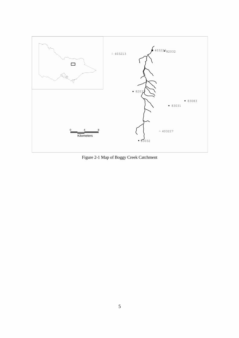
2.1 Description of the Study Catchment. The data used for testing the flood estimation procedure were from the 108 km2 Boggy Creek catchment at Angleside, station number 403226 (Hill, 1994). Hydrometric data was provided by the Bureau of Meteorology and the (former) Rural Water Corporation. There were 17 years, 1976 to 1992 inclusive, of concurrent daily rainfall and runoff for calibration of the DGAWBM continuous simulation model, and for establishing the relationship between peak rates of flow and the daily runoff values calculated by the daily rainfall-runoff model. An additional 9 years of annual maxima peak flows were available for flood frequency analysis, giving a 26-year period, 1967-1992, available for this part of the study. A 58-year period, 1935-1992, of daily rainfalls were available for calibrating the DGRAIN rainfall generator. Catchment average rainfall was calculated as the average of stations 082032, 082033, 083031 and 083032. The location of the stations are shown in Figure 2-1. It should be noted that the available rainfall was as daily data (ie restricted period) rather then 24 hour (unrestricted period) data.

5

82033

83032

40321382032403226

403227

83031

83083

0 4

Kilometers

8

Figure 2-1 Map of Boggy Creek Catchment

6

2.2 Description of the Model The model used to generate synthetic sequences of daily rainfalls is a modification of a method described by Haan et al. (1976). This method was modified for use in Australia by Srikanthan and McMahon (1985) and further modified in the present study. The model is referred to as a transition probability matrix (TPM) or a multi-state Markov chain model. Following the methodology adopted by Srikanthan and McMahon (1985) for the region of the Boggy Creek catchment, daily rainfalls are divided into 6 states as shown in Table 2-1.

Table 2-1 States of Daily Rainfall

State Rain 1 zero 2 zero < rain ≤ 0.9 mm 3 0.9 < rain ≤ 2.9 mm 4 2.9 < rain ≤ 6.9 mm 5 6.9 < rain ≤ 14.9 mm 6 14.9 < rain

The probabilities for rain in one state to be followed by rain on the next day in the same or another state are collated into a matrix - the transition probability matrix. Seasonality of rain is modelled by using 12 TPMs, one for each calendar month. The TPM for January on the Boggy Creek catchment is shown in Table 2.2. The values are percent probability of going to the next state on the following day from the current state of today's rain.

Table 2-2 Transition Probability Matrix for January

Current Next State State 1 2 3 4 5 6

1 84.3 5.6 3.7 2.7 2.3 1.4 2 59.8 18.9 6.1 7.6 3.8 3.8 3 42.5 15.2 14.1 14.1 7.6 6.5 4 54.6 4.7 7.0 12.8 12.8 8.1 5 41.3 14.3 12.7 7.9 4.8 19.0 6 43.5 8.1 6.4 8.1 12.9 21.0

2.3 Generation within each State The selection of the next state from the current state is made using a random number. Using Table 2-2 as an example, assume that the current state is 1 (i.e. zero rain). If the random number is less than or equal to 0.843, then the next state is 1. If the random number is between 0.843 and 0.843+0.056 = 0.899, then the next state is 2, etc. Within states 2 to 5, the value of the generated rainfall is determined assuming a linear variation across the range, and using the value of the random number which falls within the range of the state.

7

In state 6, the generated values have no upper limit, and a frequency distribution is used with a second random number to determine the value of the rainfall. The distribution used is the log-Boughton distribution (Boughton, 1980; Boughton and Shirley, 1983). The relationship between average recurrence interval T years and frequency factor K is given by the equation :

K A CT

T A= +

− −ln ln( )1 (2.1)

where: A is a shape parameter similar to a skew parameter; C is a function of A. Setting C = A*(A + 0.3665) forces the distribution to make K = 0.0 when T = 2 years. The mean and standard deviation are determined for each month of the year from the daily rainfalls greater than 14.9 mm in the month. The shape parameter A is determined by fitting to available calibration data, preferably including rainfall estimates in the extreme range. This is explained in the following section.

2.4 Calibration of the Model The major purpose of the model is to simulate the annual maxima daily rainfalls to reflect the actual distribution of annual maxima daily rainfalls as well as possible. Calibration of the model is demonstrated using data from the 108 sq km Boggy Creek catchment. Actual values of annual maxima daily rainfalls over the catchment in the 58 year period, 1935-1992, are shown in Table 2-3.

Table 2-3 Annual Maxima Daily Rainfalls over the Boggy Creek Catchment

Year Rain (mm)

Year Rain (mm)

Year Rain (mm)

1935 33.7 1955 79.8 1975 59.7 1936 64.2 1956 72.6 1976 26.3 1937 47.4 1957 64.3 1977 39.4 1938 45.7 1958 53.4 1978 79.7 1939 93.4 1959 65.9 1979 82.9 1940 31.7 1960 42.4 1980 66.9 1941 96.4 1961 41.7 1981 83.7 1942 56.6 1962 42.7 1982 33.5 1943 32.8 1963 67.6 1983 74.5 1944 29.0 1964 37.3 1984 74.1 1945 60.1 1965 56.0 1985 40.9 1946 45.2 1966 84.5 1986 70.5 1947 53.9 1967 27.0 1987 53.7 1948 62.1 1968 61.7 1988 76.5 1949 67.8 1969 49.6 1989 101.3 1950 62.3 1970 45.5 1990 54.2 1951 58.0 1971 46.9 1991 63.1 1952 63.4 1972 32.2 1992 61.9 1953 68.3 1973 77.8 1954 44.8 1974 97.2

Note: Rainfall totals are catchment average values

8

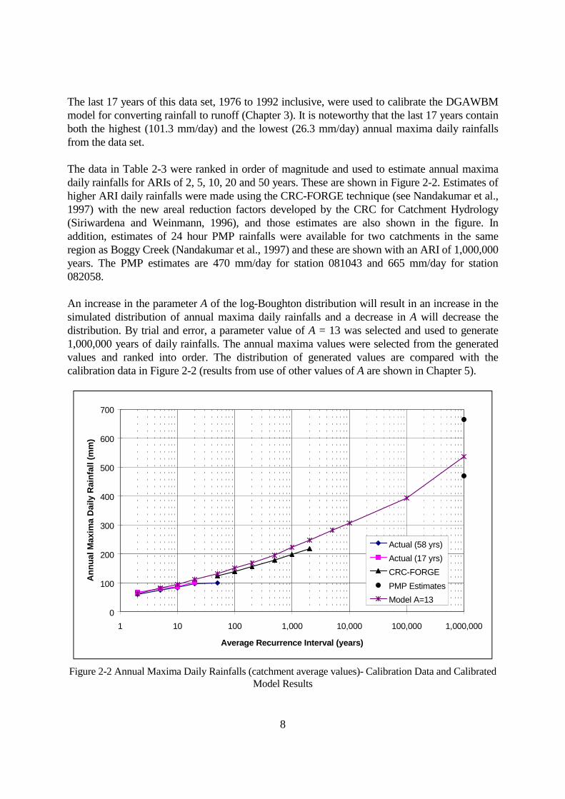
The last 17 years of this data set, 1976 to 1992 inclusive, were used to calibrate the DGAWBM model for converting rainfall to runoff (Chapter 3). It is noteworthy that the last 17 years contain both the highest (101.3 mm/day) and the lowest (26.3 mm/day) annual maxima daily rainfalls from the data set. The data in Table 2-3 were ranked in order of magnitude and used to estimate annual maxima daily rainfalls for ARIs of 2, 5, 10, 20 and 50 years. These are shown in Figure 2-2. Estimates of higher ARI daily rainfalls were made using the CRC-FORGE technique (see Nandakumar et al., 1997) with the new areal reduction factors developed by the CRC for Catchment Hydrology (Siriwardena and Weinmann, 1996), and those estimates are also shown in the figure. In addition, estimates of 24 hour PMP rainfalls were available for two catchments in the same region as Boggy Creek (Nandakumar et al., 1997) and these are shown with an ARI of 1,000,000 years. The PMP estimates are 470 mm/day for station 081043 and 665 mm/day for station 082058. An increase in the parameter A of the log-Boughton distribution will result in an increase in the simulated distribution of annual maxima daily rainfalls and a decrease in A will decrease the distribution. By trial and error, a parameter value of A = 13 was selected and used to generate 1,000,000 years of daily rainfalls. The annual maxima values were selected from the generated values and ranked into order. The distribution of generated values are compared with the calibration data in Figure 2-2 (results from use of other values of A are shown in Chapter 5).

0

100

200

300

400

500

600

700

1 10 100 1,000 10,000 100,000 1,000,000

Average Recurrence Interval (years)

Ann

ual M

axim

a D

aily

Rai

nfal

l (m

m)

Actual (58 yrs)Actual (17 yrs)CRC-FORGEPMP EstimatesModel A=13

Figure 2-2 Annual Maxima Daily Rainfalls (catchment average values)- Calibration Data and Calibrated

Model Results

9

The model closely reproduces the distribution of annual maxima daily rainfalls from the calibration data.

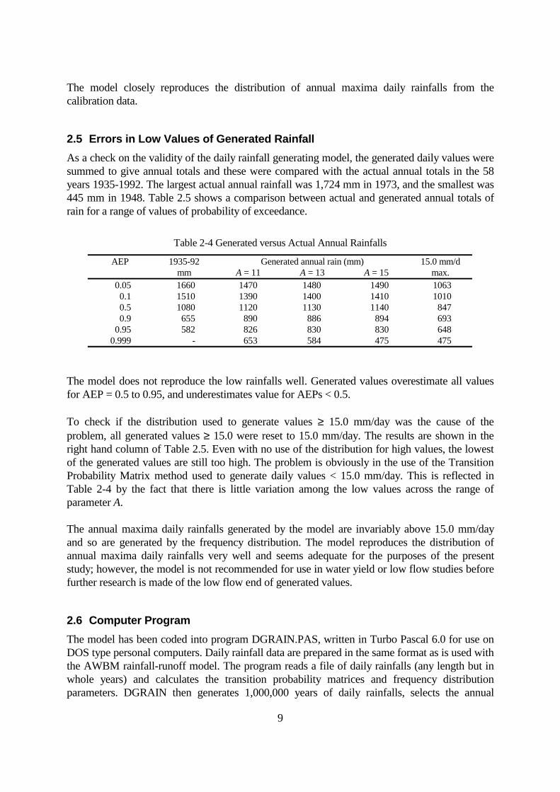
2.5 Errors in Low Values of Generated Rainfall As a check on the validity of the daily rainfall generating model, the generated daily values were summed to give annual totals and these were compared with the actual annual totals in the 58 years 1935-1992. The largest actual annual rainfall was 1,724 mm in 1973, and the smallest was 445 mm in 1948. Table 2.5 shows a comparison between actual and generated annual totals of rain for a range of values of probability of exceedance.

Table 2-4 Generated versus Actual Annual Rainfalls

AEP 1935-92 Generated annual rain (mm) 15.0 mm/d mm A = 11 A = 13 A = 15 max.

0.05 1660 1470 1480 1490 1063 0.1 1510 1390 1400 1410 1010 0.5 1080 1120 1130 1140 847 0.9 655 890 886 894 693

0.95 582 826 830 830 648 0.999 - 653 584 475 475

The model does not reproduce the low rainfalls well. Generated values overestimate all values for AEP = 0.5 to 0.95, and underestimates value for AEPs < 0.5. To check if the distribution used to generate values ≥ 15.0 mm/day was the cause of the problem, all generated values ≥ 15.0 were reset to 15.0 mm/day. The results are shown in the right hand column of Table 2.5. Even with no use of the distribution for high values, the lowest of the generated values are still too high. The problem is obviously in the use of the Transition Probability Matrix method used to generate daily values < 15.0 mm/day. This is reflected in Table 2-4 by the fact that there is little variation among the low values across the range of parameter A. The annual maxima daily rainfalls generated by the model are invariably above 15.0 mm/day and so are generated by the frequency distribution. The model reproduces the distribution of annual maxima daily rainfalls very well and seems adequate for the purposes of the present study; however, the model is not recommended for use in water yield or low flow studies before further research is made of the low flow end of generated values.

2.6 Computer Program The model has been coded into program DGRAIN.PAS, written in Turbo Pascal 6.0 for use on DOS type personal computers. Daily rainfall data are prepared in the same format as is used with the AWBM rainfall-runoff model. The program reads a file of daily rainfalls (any length but in whole years) and calculates the transition probability matrices and frequency distribution parameters. DGRAIN then generates 1,000,000 years of daily rainfalls, selects the annual

10

maxima from each year, sorts the annual maxima values, and shows the generated value for the range of ARI from 2 to 1,000,000 years.

2.7 Summary The daily rainfall generating model can be calibrated to match other estimates of annual maxima daily rainfalls over a range of ARIs from 2 to 1,000,000 years (assumed ARI for the PMP). The annual maxima daily rainfalls from 1,000,000 years of generated data were ranked and summarised into a distribution. This distribution matched well with actual data from the 58 years of daily rainfall record, with CRC-FORGE estimates in the ARI range 50 to 2000 years, and with estimates of daily PMPs from nearby catchments. A single parameter (A) is easily adjusted by trial and error to fit the generation model to the available calibration data.

11

3. DAILY RAINFALL-RUNOFF MODEL The daily rainfall generating model described in Chapter 2 can readily generate 1,000,000 years of daily rainfalls. A calibrated daily rainfall-runoff model can convert these rainfalls into 1,000,000 years of daily runoff values. The rainfall-runoff model described in this chapter is a slightly modified version of the AWBM water balance model. A new method of calibrating the model is introduced to improve the modelling of daily flows, particularly the higher values which form the annual maxima distribution of daily runoff. A comparison is made of annual maxima values of daily rainfall and daily runoff in the generated data, and this identifies an important aspect of "losses" which is not usually considered in current design flood estimation.

3.1 A Note on Terminology The terminology in common use to identify ‘losses’ and ‘rainfall excess’ in flood estimation is confusing when applied to continuous rainfall-runoff modelling, e.g. the term ‘losses’ usually includes baseflow recharge which can comprise the majority of runoff in some catchments. To avoid confusion, the following terms and symbols are defined in relation to the DGAWBM model used in this report (refer to Figure 3-1: Structure of the DGAWBM). • Storage excess XS[X]: the amount of runoff generated by overflow of surface store [X].

Storage excess contains both baseflow recharge and surface runoff (i.e. rainfall excess). • Rainfall excess RXS: the surface runoff component of storage excess. This definition retains

compatibility with the common use of the term to mean the amount of rainfall that appears as surface runoff in time periods of a few hours to a few days.

• Baseflow recharge BR: the component of storage excess that recharges the baseflow store. • Surface runoff Qs: the routed hydrograph of rainfall excess. • Baseflow Qb: discharge from the baseflow store. • Baseflow recharge fraction BRF[x] : the fraction of storage excess generated from store[x]

that becomes baseflow recharge. A different baseflow recharge fraction is used for each of the three surface stores. (0 ≤ BRF[x] ≤ 1)

• Baseflow index BFI : the ratio of the amount of baseflow in total runoff divided by the total

amount of runoff. This is usually calculated over the total period of runoff record that is available and represents the weighted average of BRF[X] over the three separate stores. (0 ≤ BFI ≤ 1)

• Daily runoff Q : Actual daily runoff is the runoff that is routed by its movement through the

catchment to where it is measured at the catchment outlet. Calculated daily runoff is the sum of the routed discharges from the surface and baseflow routing stores.

12

Figure 3-1 Structure of the DGAWBM

3.2 The DGAWBM Model The AWBM is an explicit water balance model (Boughton, 1993,1996) which simulates losses and runoff from a catchment area at either hourly or daily time steps. Runoff is generated by overflow from one or more of the surface stores, simulating saturation overland flow as the runoff generating process. The three surface stores have different storage capacities and simulate partial area runoff. The original AWBM model partitions storage excess into rainfall excess (unrouted surface runoff) and baseflow recharge using the baseflow index (BFI). If the amount of storage excess is XS, then XS*BFI becomes baseflow recharge, and XS*(1.0-BFI) becomes rainfall excess. In the original model, the division between baseflow recharge and rainfall excess is the same for all runoff events. There is evidence available (e.g. see Sharifi, 1996) that the partitioning of storage excess between baseflow recharge and rainfall excess is not constant in all runoff events. The available evidence indicates that the fraction of storage excess going into baseflow recharge is larger in small runoff events and smaller in large runoff events. The difference is not important in water yield studies where calculated runoff is accumulated into monthly totals for design of water supply works. However, the use of a constant such as BFI to partition all storage excess is not accurate enough for flood estimation studies. To improve the accuracy of the calculation of daily runoff values, the fraction of storage excess which becomes baseflow recharge has been made dependent on which surface store produces

13

the storage excess. It should be noted that storage excess is always produced from the store with smallest capacity before or at the same time as from the other stores, and from the store with largest capacity after or at the same time as from the other stores. If the baseflow recharge fraction for the smallest store is given a high value, then a larger fraction of storage excess becomes baseflow recharge in small runoff events, and if the baseflow recharge fraction for the store with largest capacity is given a small value, then more of the storage excess becomes rainfall excess in big runoff events (when all stores are producing runoff). Figure 3-1 shows the structure of the DGAWBM (Data Generation AWBM) which uses different baseflow recharge fractions for the three surface stores. This is the only difference between the DGAWBM and the original AWBM.

3.3 Calibration of the DGAWBM The structure of the original AWBM was devised to enable calibration of its parameters from simple and direct procedures, such as the partitioning of streamflow into surface runoff and baseflow to evaluate the baseflow index. The additional parameters in the DGAWBM negate some of this simplicity, and some additional procedures are needed for calibration. The partitioning of streamflow into surface runoff and baseflow is still used as a start. DGBFLOW is very similar to the streamflow partitioning program NEWBFLOW used with the original AWBM (Boughton, 1996). For flood estimation purposes, it is essential to file the results of flow partitioning into a file named PARTFLOW, which contains the surface runoff and baseflow components of each daily flow, and to save the parameter values for baseflow index BFI and the daily baseflow recession constant K into a parameter file named DGPARAM.#$&. These procedures are built into DGBFLOW. The saving of these results and parameters is necessary because they are used by later programs. Preliminary calibration of the DGAWBM parameters is then made using the program DGBASE5. This program reads the parameter file DGPARAM.#$& to get initial values of the baseflow index BFI and the daily baseflow recession constant K. DGBASE5 gives a preliminary calibration of the surface storage capacities C1, C2 and C3 and the partial areas of these stores A1, A2 and A3. Also, the surface runoff routing constant KS can be manually adjusted using the screen plots of actual and calculated daily flows. The parameter values from this preliminary calibration are saved by overwriting the file DGPARAM.#$&. The main calibration is then made using the program DGCALIBR. This program uses a multi-objective calibration function to maintain a proper division of streamflows into surface runoff and baseflow, and also ensures that the calculated maximum daily flows in each month best match the actual set of maximum daily flows. The multi-objective function is calculated as follows.

(i) For each trial set of parameter values, the program calculates the surface runoff, baseflow and maximum daily flow in each month.

(ii) For each of these 3 variables, a linear regression forced through the origin is calculated between actual and calculated values, and the correlation coefficient (CC) and the slope (S) of the regression line are determined.

14

(iii) If the slope is less than 1.0, then the function CC*S is calculated. If the slope is greater than 1.0, then the function CC/S is calculated.

(iv) The product of the functions of the 3 variables is then maximised to ensure that the correlation coefficients are as high as possible while maintaining the slopes of the regressions as close to 1.0 as possible.

As an example, the calculated values of the slopes and correlation coefficients for a given set of parameter values are shown in Table 3-1.

Table 3-1 Sample Calculation of Calibration Function

Correlation Regression Coefficient Slope Surface Runoff 0.92 1.05 Baseflow 0.94 0.90 Max Day Flows 0.88 0.93

The calibration function for this run would be : (0.92/1.05)*(0.94*0.90)*(0.88*0.93) = 0.607

DGCALIBR adjusts the parameter values by trial and error to find the highest possible value of the calibration function. The program decreases the incremental changes in parameter values after each run so that smaller incremental changes are gradually tested. There are opportunities to fix values for chosen parameters, set starting values for parameters and each increment, and to control the length of the trial and error search. The multi-objective calibration function maintains the division of flow into surface runoff and baseflow while seeking the best match between actual and calculated monthly maxima daily flows. The results from the Boggy Creek catchment illustrate the calibration procedure. The DGBFLOW program gave values of K = 0.952 for the baseflow daily baseflow recession constant, and BFI = 0.60 for the baseflow index. When the DGBASE5 program was run, the daily recession constant changed to 0.97 and the daily recession constant for the surface runoff store was 0.40. The capacities and partial areas of the surface stores became :

Table 3-2 Preliminary Calibration of Stores by DGBASE5

Capacity (mm)

Partial Area

Store 1 10 0.208 Store 2 260 0.520 Store 3 520 0.272

The coefficient of determination between actual and calculated monthly totals of runoff at this stage was 0.947. Using these preliminary results as starting values, the program DGCALIBR produced the following set of calibrated parameter values :

15

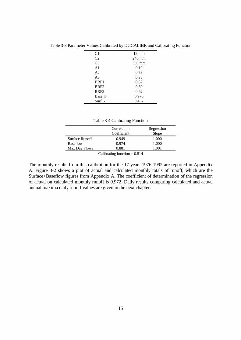
Table 3-3 Parameter Values Calibrated by DGCALIBR and Calibrating Function

C1 13 mm C2 246 mm C3 503 mm A1 0.19 A2 0.58 A3 0.23 BRF1 0.62 BRF2 0.60 BRF3 0.62 Base K 0.970 Surf K 0.437

Table 3-4 Calibrating Function

Correlation Coefficient

Regression Slope

Surface Runoff 0.949 1.000 Baseflow 0.974 1.000 Max Day Flows 0.881 1.001

Calibrating function = 0.814 The monthly results from this calibration for the 17 years 1976-1992 are reported in Appendix A. Figure 3-2 shows a plot of actual and calculated monthly totals of runoff, which are the Surface+Baseflow figures from Appendix A. The coefficient of determination of the regression of actual on calculated monthly runoff is 0.972. Daily results comparing calculated and actual annual maxima daily runoff values are given in the next chapter.

16

0

50

100

150

200

250

0 50 100 150 200 250

Calculated Monthly Runoff (mm)

Act

ual M

onth

ly R

unof

f (m

m)

Figure 3-2 Actual versus Calibrated Monthly Runoff from Calibrated DGAWBM

(Boggy Creek, 1976-1992)

17

3.4 Generation of Daily Runoff Program DGRUNOFF contains the daily rainfall generation model (as in DGRAIN) plus the code for the DGAWBM daily rainfall-runoff model. Generated daily rainfalls are used as input to the rainfall-runoff model and daily runoff values are calculated. The daily rainfall generating model requires a setting of the frequency distribution parameter A, as in DGRAIN. The DGAWBM parameters were set according to Table 3-3. The annual maxima daily runoff values are selected and ranked in order as a frequency distribution in the same manner as rainfalls are treated in DGRAIN. The annual maxima daily rainfalls and runoff for A = 13 are shown in Table 3-5.

Table 3-5 Generated Rainfall and Runoff for A = 13.0

ARI (years)

Rain (mm/day)

Runoff (mm/day)

1,000,000 537 126 500,000 428 101 200,000 399 97.0 100,000 392 91.6 50,000 369 84.6 20,000 336 77.1 10,000 306 71.3 5,000 282 65.1 2,000 248 57.8 1,000 223 52.2

500 195 47.1 200 170 40.8 100 151 36.6 50 132 32.7 20 112 28.3 10 96 24.7 5 82 21.4 2 62 16.9

3.5 Losses It should be noted that the runoff values in Table 3-5 comprise surface runoff routed through the surface runoff store and baseflow which is a routed outflow from the baseflow store. The difference between rainfall and runoff does not represent a loss. This is because the rainfall and runoff are selected as annual maxima independent of each other, and the rankings into the two distributions are made without reference between the values. A closer comparison between rainfall and runoff can be made by setting the surface runoff routing parameter to zero. This makes each daily input to the surface routing store become outflow, i.e. there is no routing or attenuation of the rainfall excess. The calculations used to produce Table 3-5 were repeated with the surface routing parameter set to zero. The new results are shown in Table 3-6. As mentioned before, the annual maxima

18

rainfalls and annual maxima daily runoff are selected independently of each other and may not occur on the same day (but are likely to). It should be noted that the rainfall for a particular ARI in Table 3-6 is slightly different to that given in Table 3-5 and is the result of generating a new set of rainfall data using different random numbers.

Table 3-6 Generated Rainfall and Unrouted Surface Runoff for A = 13.0

ARI (years)

Rain (mm/day)

Unrouted Runoff (mm/day)

Ratio

1,000,000 574 242 0.42 500,000 491 211 0.44 200,000 437 182 0.42 100,000 417 169 0.41 50,000 366 152 0.42 20,000 330 135 0.41 10,000 306 124 0.41 5,000 282 113 0.40 2,000 246 99.4 0.40 1,000 223 90.0 0.40

500 202 81.3 0.40 200 173 69.5 0.40 100 152 61.2 0.40 50 137 55.2 0.40 20 114 46.3 0.41 10 97.5 39.6 0.41 5 82.2 34.7 0.42 2 61.6 26.1 0.42

The constancy of the ratio of runoff to rainfall, about 0.4, shows the dominance of baseflow recharge in determining "loss" and the amount of surface runoff. If all of the 3 surface stores were full at the start of the day, then the baseflow recharge would be 0.608 and the surface runoff 0.392 of the storage excess (based on the values in Table 3-3). Discharge from the baseflow store is added to the surface runoff to give the calculated daily runoff. A study of the calculated annual maxima values showed that all stores were full and generating runoff for ARIs of 5 years and greater, i.e. partial area runoff did not affect the main pattern of calculated annual maxima daily runoff. The small variation among the ratios of runoff/rainfall in Table 3-5 shows that the 0.608 of storage excess going into baseflow recharge is virtually the sole determinant of the calculated annual maxima daily runoff values, and, as a consequence, the estimated annual maxima peak flood flows. If the baseflow recharge fraction of storage excess dropped by one-half, from 0.6 to 0.3, in very large runoff events, then the calculated surface runoff would increase by 75%. There is no information available as to how baseflow recharge varies as storm rainfall and runoff increase. The data available for calibration of the rainfall-runoff model show a relatively constant fraction of storage excess becoming baseflow recharge. Because of the importance in determining flood peaks, some direction of research effort to the matter is warranted.

19

3.6 Summary The modification made to the structure of the AWBM model proved to be unnecessary, and the results could readily have been obtained from the original model. The new calibration method was very successful, with potential for use in other rainfall-runoff studies. The results from comparing 1,000,000 years of generated runoff with generated rainfall show that baseflow recharge was the dominant factor in determining "loss" and the amount of surface runoff. The results highlight the need for more information about how baseflow recharge varies as storm rainfall and runoff increase.

20

4. RELATING PEAK FLOW RATES TO VOLUME OF RUNOFF Peak rates of runoff have been related to volume of runoff in a number of ways in previous studies. A brief review of the most relevant studies is given in the following section. The effects of using different forms of relationship, e.g. log-log versus natural values, is examined, and the effects of the differences are reported. The method using a log-log relationship is selected for use in this study.

4.1 Previous Work on Peak/Volume Ratios As early as 1914, Fuller proposed an equation to convert maximum average 24 hour flood discharge to peak discharge : ( )Q Q A= + −

240 3 2

1 2 . (4.1)

where: Q = peak discharge; Q24 = maximum average 24 hour discharge; A = catchment area. The Boggy Creek catchment is 108 km2 = 41.7 mi2, for which Fuller's equation gives a Peak/Vol ratio of 2.73. The actual ratio (see later in this chapter) is 2.1, ie. Fuller's equation overestimates peak discharges by 30% on this catchment. For small arid catchments with brief ephemeral periods of runoff, Renard et al. (1970) found the coefficient of determination between peak discharges and total event runoff to be highly significant. Rogers (1980) and Rogers and Zia (1982) also related flood peaks to hydrograph volume. Bradley and Potter (1992) related 3 day flow volume to peak flows on large catchments where the 3 day volume was appropriate. Watt (1971) derived a relationship between peak discharge and maximum 24 hour flows on 13 catchments ranging from 39 to 1,342 sq. km in area. Boughton (1975,1976) related the frequency distribution of recorded annual maxima flood peaks to the frequency distribution of annual maxima calculated daily runoff values using a daily rainfall-runoff model. Calculated daily runoff was used in lieu of actual daily runoff because the purpose was to use the rainfall-runoff model with long periods of daily rainfalls to extend short records of actual flood peaks. The relationship was established between frequency distributions of annual maxima data because the end result was a long term frequency distribution of peaks estimated from the annual maxima frequency distribution of calculated daily runoff values. The relationship is a statistical relationship and not a deterministic relationship between peak and daily volume from specific events.

4.2 Testing of Methods In the present study, the method used by Boughton (1975, 1976) was used with some slight modifications. The main modification of the original method is that the calibration of the model

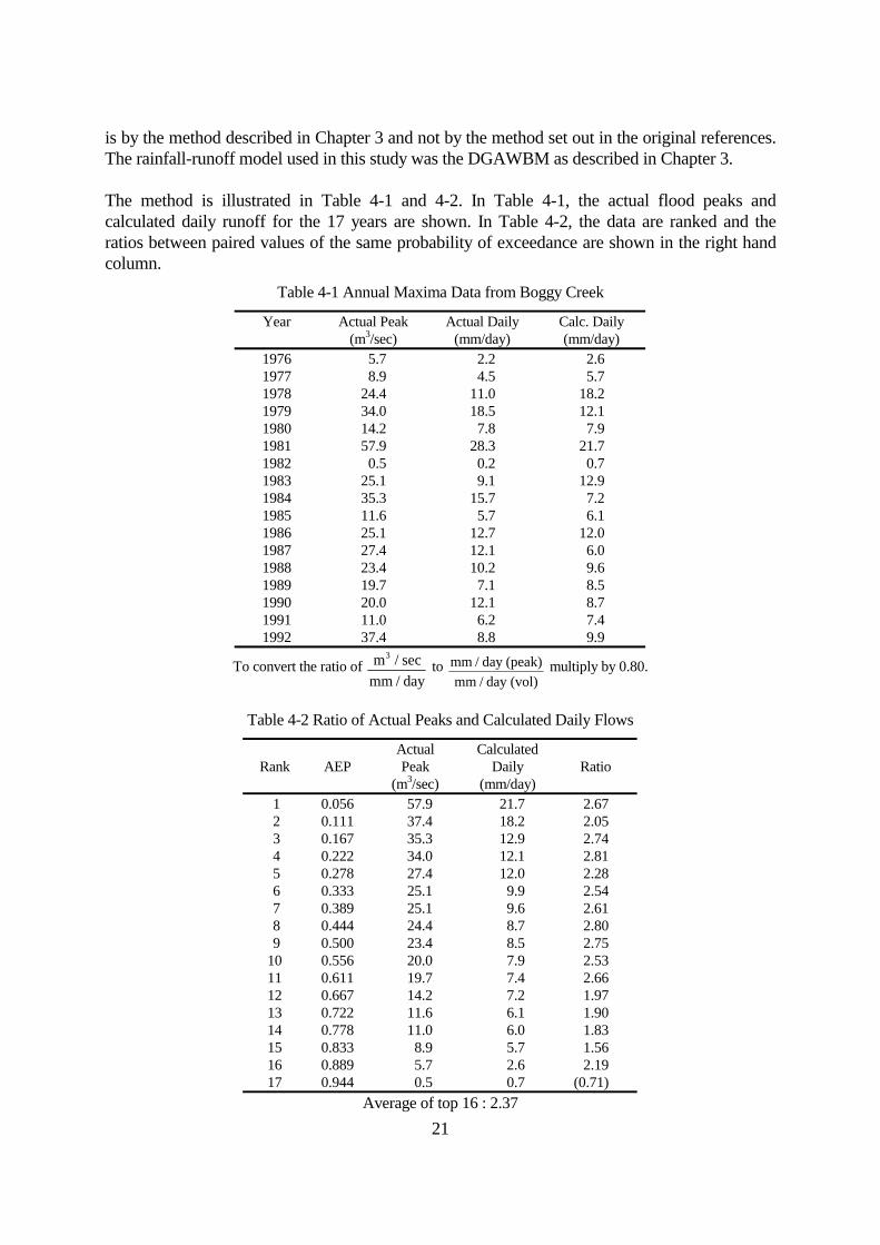
21

is by the method described in Chapter 3 and not by the method set out in the original references. The rainfall-runoff model used in this study was the DGAWBM as described in Chapter 3. The method is illustrated in Table 4-1 and 4-2. In Table 4-1, the actual flood peaks and calculated daily runoff for the 17 years are shown. In Table 4-2, the data are ranked and the ratios between paired values of the same probability of exceedance are shown in the right hand column.

Table 4-1 Annual Maxima Data from Boggy Creek

Year Actual Peak (m3/sec)

Actual Daily (mm/day)

Calc. Daily (mm/day)

1976 5.7 2.2 2.6 1977 8.9 4.5 5.7 1978 24.4 11.0 18.2 1979 34.0 18.5 12.1 1980 14.2 7.8 7.9 1981 57.9 28.3 21.7 1982 0.5 0.2 0.7 1983 25.1 9.1 12.9 1984 35.3 15.7 7.2 1985 11.6 5.7 6.1 1986 25.1 12.7 12.0 1987 27.4 12.1 6.0 1988 23.4 10.2 9.6 1989 19.7 7.1 8.5 1990 20.0 12.1 8.7 1991 11.0 6.2 7.4 1992 37.4 8.8 9.9

To convert the ratio of m / secmm / day

3 to mm / day (peak)

mm / day (vol) multiply by 0.80.

Table 4-2 Ratio of Actual Peaks and Calculated Daily Flows

Rank

AEP

Actual Peak

(m3/sec)

Calculated Daily

(mm/day)

Ratio

1 0.056 57.9 21.7 2.67 2 0.111 37.4 18.2 2.05 3 0.167 35.3 12.9 2.74 4 0.222 34.0 12.1 2.81 5 0.278 27.4 12.0 2.28 6 0.333 25.1 9.9 2.54 7 0.389 25.1 9.6 2.61 8 0.444 24.4 8.7 2.80 9 0.500 23.4 8.5 2.75 10 0.556 20.0 7.9 2.53 11 0.611 19.7 7.4 2.66 12 0.667 14.2 7.2 1.97 13 0.722 11.6 6.1 1.90 14 0.778 11.0 6.0 1.83 15 0.833 8.9 5.7 1.56 16 0.889 5.7 2.6 2.19 17 0.944 0.5 0.7 (0.71)

Average of top 16 : 2.37

22

The average of the Peak(m3/sec)/Vol(mm/day) ratios for the highest 16 pairs of values is 2.37. The smallest pair of values occurred in a very dry year (1982) when the highest flow in the entire year was only 0.475 m3/sec. The ratio can vary widely on such small values so the lowest value is excluded when calculating the average value. The ratio between the two frequency distributions is illustrated in Figure 4-1.

0.1

1

10

100

Annual Exceedance Probability

Actual Peaks (m ³/s)

Calculated Daily Volum es (m m /day)

0.90.95 0.30.50.6 0.10.2 0.010.020.050.40.7

Ratio2.37

0.8

Figure 4-1 Peak/Volume Ratio from Comparison of Frequency Distributions

An alternative method of calculating the average ratio to is fit a linear regression to the pairs of values with the line forced through the origin. The slope of the regression line through the origin is the required ratio of Peak/Vol. The equation for calculating the ratio in this way is :

Ratio = ∑∑

xyx2 (4.2)

where: x = daily volume of given ARI; y = peak flow of same ARI. The slope of the regression line for the data in Table 4-1 is 2.47 and this is illustrated in Figure 4-2. The reason for the higher value from this alternate method is that the high ratios of the higher data pairs have more effect on the regression line that on the average calculated by the first method. An advantage of this approach is that very small values such as the lowest data pair from 1982 have very little effect on the regression slope and do not have to be specifically excluded from the calculation.

23

0

10

20

30

40

50

60

70

0 5 10 15 20 25

Calculated Daily Flow (mm/day)

Regression line through originPeak = 2.47 x Volume

Fitted regressionPeak = -1.75 + 2.62 x Volume

Figure 4-2 Peak/Vol Ratio from Fitted Linear Regression

There is a tendency for the ratio to be higher with the higher ARI values and lower with lower ARI values. If the regression is not forced through the origin, the regression equation becomes Peak (m3/sec) = -1.75 + 2.62*Vol (mm/day). For very high values of runoff volume, the constant -1.75 becomes insignificant, and the equation implies a ratio of peak to volume of 2.62. The tendency for a higher ratio with higher ARI is more evident if the Peak/Vol regression is based on logs instead of natural values. Excluding the lowest pair of values (as in Table 4-2) and using base 10 logs of the data, the fitted regression becomes log Peak = 0.224 + 1.153*log Vol, which is equivalent to Peak = 1.675*Vol1.153. The log-log regression is shown in Figure 4-3.

Peak = 1.675 x Volume1.153

1

10

100

1 10 100

Calculated Daily Runoff (mm/day)

Peak

Flo

w R

ate

(m³/s

)

m³/s mm/day

Figure 4-3 Peak/Volume Ratio from log-log Linear Regression

24

Because the exponent (1.153) is greater than unity, the Peak/Vol ratio increases as the volume of calculated daily runoff increases (indicating the non-linear reponse of this catchment). The range of values of the ratio is illustrated in Table 4.3 using values of calculated daily runoff from Table 5.2 (next chapter). The ratio is much the same as found in the previous regression when the runoff values are of similar magnitude as the actual data, in the range of ARI 2 to 10 years. The ratio increases significantly for the higher values of calculated runoff at ARIs greater than 100 years.

Table 4-3 Peak/Vol Ratios Based on Log-Regression

ARI (years)

Runoff for A = 13 (mm/day)

Ratio

100,000 91.6 3.34 10,000 71.3 3.22 1,000 52.2 3.07

100 36.6 2.90 10 24.7 2.74 2 16.1 2.58

The use of a relationship based on logs instead of natural values is speculative because there are no data available on Peak/Vol ratios for ARI > 100 years. The calculated ratios are 25-30% higher than the fixed ratio of 2.6 for ARIs 10,000 to 100,000 years. The conservative nature of the higher ratios has some appeal because of the uncertainties involved in estimating floods at high ARI. It is suggested that all of these methods be used in practice and that the results be plotted as in Figures 4.1, 4.2 and 4.3 in order to give the maximum amount of information about the ratio and how each of the data pairs are affecting the results. For this study, the higher ratios from the log-log regression are adopted for the estimation of peak flows in m3/sec from calculated values of annual maxima daily runoff in mm/day.

4.3 Summary The three methods which were examined for establishing a ratio of peak flow rate to daily volume of runoff gave results which varied from 2.37 for a simple averaging of ratios from the ranked sets of data, to 2.62 for a fitted linear regression between natural values, and then to a range, 2.58 to 3.34, when logarithms of the data were used to fit a regression. The log-log relationship gave highest values of the ratio at the highest ARIs, and so gives the highest estimates of peak flow rates for ARIs > 10 years. Because of the uncertainties which are inherent in estimates of floods with high ARIs, the log-log relationship is the most conservative of the three methods tested, and so is adopted for use in this study.

25

5. RESULTS The components of the new design flood estimation procedure, i.e. daily rainfall generating model (Chapter 2), rainfall-runoff model (Chapter 3) and peak/volume relationship (Chapter 4), are brought together in this chapter to demonstrate a complete application with the data from the Boggy Creek study catchment. The single parameter (A) in the daily rainfall generating model must be calibrated by trial and error against available information on annual maxima daily rainfalls, hence the effect of this parameter on results is illustrated through the chapter. The results from the new procedure are compared with results from fitting frequency distributions to the raw data, and with a general estimate of the PMF.

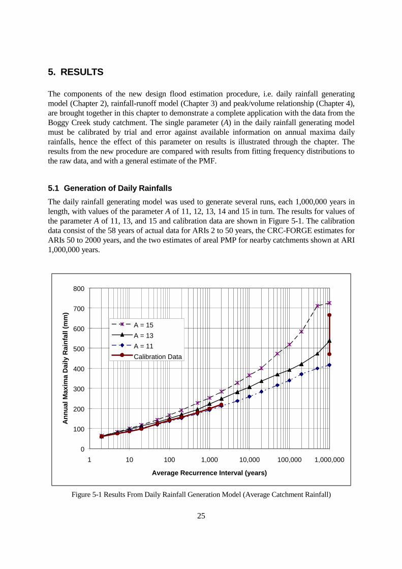
5.1 Generation of Daily Rainfalls The daily rainfall generating model was used to generate several runs, each 1,000,000 years in length, with values of the parameter A of 11, 12, 13, 14 and 15 in turn. The results for values of the parameter A of 11, 13, and 15 and calibration data are shown in Figure 5-1. The calibration data consist of the 58 years of actual data for ARIs 2 to 50 years, the CRC-FORGE estimates for ARIs 50 to 2000 years, and the two estimates of areal PMP for nearby catchments shown at ARI 1,000,000 years.

0

100

200

300

400

500

600

700

800

1 10 100 1,000 10,000 100,000 1,000,000

Average Recurrence Interval (years)

Ann

ual M

axim

a D

aily

Rai

nfal

l (m

m)

A = 15A = 13A = 11Calibration Data

Figure 5-1 Results From Daily Rainfall Generation Model (Average Catchment Rainfall)

26

Because only a single run of 1,000,000 years was made for each value of A, the rainfall values for the higher ARIs show noticeable variation; for example, the ‘kink’ in the curve for an A of 15 between an ARI of 500,000 and 1,000,000 years. Each 1,000,000 year run of generated values contains only one estimate of the value for an ARI of 1,000,000 years, 10 estimates of the value for an ARI of 100,000 years, 100 estimates for an ARI of 10,000 years and 1000 estimates for an ARI of 1000 years; hence the generated values for an ARI of 10,000 years and less are more consistent, and those for high ARIs are less consistent. In Figure 5-1 a value of A = 11 best reproduces the calibration data for ARIs up to 2000 years, i.e. the actual data values and the CRC-FORGE estimates. This value for A gives low estimates for the PMP rainfall at ARI = 1,000,000 years. A higher value of A of 13 gives a better estimate of the PMP rainfall but slightly higher values than the CRC-FORGE estimates between 50 and 2000 years ARI.

5.2 Generation of Daily Runoff The calibrated parameter values of the rainfall-runoff model, given in Table 3-3, were used in program DGRUNOFF to generate annual maxima daily runoff values. The parameter A in the daily rainfall generation model was varied from 11 to 15 as before. In each run, 1,000,000 years of daily runoff values were generated and the annual maxima values selected. The values of generated runoff increase as the parameter A in the rainfall generating model is increased. Table 5-1 summarises the generated daily runoff values.

Table 5-1 Results from Daily Runoff Generation Model

ARI Annual Maxima Daily Runoff mm/day for A = (years) 11 12 13 14 15

1,000,000 103 112 126 126 163 500,000 83.3 107 101 125 157 200,000 81.3 96.2 97.0 113 134 100,000 77.0 90.7 91.6 106 116 50,000 71.3 82.6 84.6 97.7 108 20,000 64.0 71.5 77.1 87.6 91.3 10,000 59.8 64.7 71.3 80.4 84.1 5,000 55.7 59.5 65.1 72.2 76.6 2,000 49.8 53.0 57.8 62.9 66.2 1,000 45.7 48.3 52.2 56.6 59.3

500 41.4 43.9 47.1 49.6 52.5 200 36.7 38.7 40.8 42.6 45.3 100 33.3 34.8 36.6 38.5 40.3 50 30.4 30.7 32.7 34.9 35.5 20 26.6 27.0 28.3 29.2 29.6 10 23.5 23.9 24.7 25.5 25.9 5 20.4 21.0 21.4 21.9 22.4 2 16.6 16.7 16.9 16.9 17.4

27

5.3 Estimation of Peak Rates of Runoff Annual maxima peak rates of runoff are estimated by multiplying the daily runoff values in Table 5-1 by the Peak/Vol ratios established in Chapter 4. For this study, the higher ratios found in the log-log regression of Peak on Volume were used. The reason for this choice is that the calculated daily runoff values are strongly influenced by the baseflow recharge process in the model (see Chapter 3) leading to a relatively constant ratio between rainfall excess and daily rainfall. The Peak/Vol ratios based on the log-log regression increase with increasing ARI and hence offset the constant ratio of daily rainfall excess to daily rainfall. The peak rates of flow in Table 5-2 were calculated by multiplying the daily runoff values in Table 5-1 by the Peak/Volume ratios summarised in Table 4-3. The results in Table 5-2 show that the value of parameter A in the daily rainfall generating model has very little effect on the calculated peak rates of runoff at low ARI values and only moderate effect at high ARI values. An increase of 1 in the value of A increases the estimate of peak rate of runoff by about 5% at an ARI of 100 years and by about 12% at an ARI of 1,000,000 years.

Table 5-2 Estimates of Peak Rates of Runoff

ARI Annual Maxima Peak Flows m3/sec for A = (years) 11 12 13 14 15

1,000,000 349 385 443 440 595 500,000 274 368 343 438 569 200,000 267 324 327 389 474 100,000 251 303 306 360 403 50,000 229 272 279 330 371 20,000 203 230 251 291 305 10,000 187 205 229 263 278 5,000 173 186 207 233 249 2,000 152 163 180 199 211 1,000 137 146 160 176 186

500 123 131 142 151 161 200 107 113 121 127 136 100 95 100 106 113 119 50 86 87 93 101 103 20 74 75 79 82 83 10 64 65 68 70 71 5 54 56 57 59 60 2 43 43 44 44 45

The choice of value for parameter A is subjective and depends on the data available for calibration - see Figure 5-1. A value of A = 13 is chosen for the Boggy Creek data in this study because it slightly over-estimates the CRC-FORGE estimates of daily rainfalls in the ARI range 50 to 2000 years but gives reasonable agreement with the available PMP data from nearby catchments. The results for A = 13 in the above table therefore represent the estimated flood frequency distribution for the Boggy Creek catchment.

28

5.4 Comparison with Frequency Analysis of Observed Flood Peaks The estimates of peak rates of runoff in Table 5-2 are compared with frequency analysis of two periods of data from the Boggy Creek catchment. In the first instance, frequency distributions were fitted to annual maxima flood peaks from the 17 years 1976-1992 which were used to calibrate the daily rainfall-runoff model. Then the same distributions were fitted to a longer period of data the 26 years from 1967 to 1992. Three distributions were fitted to the data sets

(i) the log-Pearson 3 using the procedures and frequency factors in Australian Rainfall and Runoff (Pilgrim, 1987);

(ii) the log-Boughton distribution (Boughton, 1980, Boughton and Shirley, 1983);

(iii) the GEV distribution fitted by the method of higher order L moments (Wang, 1996a,b). The use of the different distributions demonstrates that factors such as low flood values and length of available data have far more effect on flood estimates than the choice of distribution. The recorded annual maxima floods used in these analyses are given in Table 5-3.

Table 5-3 Recorded Annual Maxima Flood Peaks (m³/sec) Boggy Creek catchment

Year Peak Year Peak Year Peak 1967 4.0 1976 5.7 1985 11.6 1968 56.1 1977 8.9 1986 25.1 1969 6.5 1978 24.4 1987 27.4 1970 46.9 1979 34.0 1988 23.4 1971 11.7 1980 14.2 1989 19.7 1972 2.3 1981 57.9 1990 20.0 1973 23.5 1982 0.5 1991 11.0 1974 90.2 1983 25.1 1992 37.4 1975 45.4 1984 35.3

(a) 17 years 1976-1992 The first problem demonstrated in this data set is the effect of one or more very low recorded flood values on the estimated values of high ARI floods. In the 17 years, 1976-1992, a very dry year occurred in 1982, resulting in an annual maximum flood of only 0.5 m3/sec in that year. Using all 17 years of data, the parameters for fitting of the frequency distribution were mean = 1.22, standard deviation = 0.465, and skew = -2.32 (using base 10 logarithms of the data). The very low flood in 1982 has a big effect on the coefficient of skewness which, in turn, substantially reduces the high values of the fitted distributions. Table 5-4 shows the results from fitting the two distributions to all data in the 17 years. The effect of the single low value in 1982 is to make the estimates of the 100 year ARI (and even 500 year ARI) flood less than the highest value in the 17 years of data with either of the distributions.

29

Table 5-4 Peak Flood Estimates (in m³/sec) from 17 years of Observed Data (1976-1992)

ARI All Data Lowest N values omitted GEV (years) LB LPIII 1 2 3 fitted by

LB LPIII LB LPIII LB LPIII LH-moments 100 43 41 63 65 63 67 62 66 70 50 41 41 57 59 58 59 57 58 60 10 36 39 42 42 42 41 42 41 40 5 32 36 34 33 34 33 34 33 32 2 23 24 21 20 21 21 21 21 21

Such effects of low flood values on the fitting of frequency distributions are commonplace. The use of the log-Boughton distribution to compare with the more common log-Pearson III is because Boughton and Shirley (1983) set out a procedure for exact fitting of that distribution to subsets of data, whereas the procedure in AR&R for fitting of the log-Pearson III to a subset of data is an empirical adjustment of the probabilities of exceedance. Both methods produce similar results. The discarding of the lowest value from the data set increases the estimate of the 100 year ARI flood by more than 50% whereas the choice of distribution makes very little change. Also shown in Table 5-4 are the results from fitting a GEV distribution by the method of higher order L moments which gives more weight to the largest events (Wang, 1996a,b). The advantage of using higher order moments is that there is no need to make a subjective decision on the number of low values to exclude. The fitted distribution is shown in Figure 5-2.

Figure 5-2 Fitted GEV Distribution using LH-Moments for 1976-1992

30

(b) 26 years 1967-1992 The second problem which is demonstrated here is the difference in estimates produced by introducing an additional period of data. The highest flood in the 17-year period was 57.9 m3/sec in 1981. The additional 9 years of data contain a flood of 90.2 m3/sec in 1974 and a flood of 56.1 m3/sec in 1968. The additional floods give a substantial increase in estimates of high ARI floods when the whole data set is used, and even higher when low values are discarded - see Table 5-5. The GEV distribution fitted by higher order L-moment is also shown and the fitted distribution is shown in Figure 5-3.

Table 5-5 Peak Flood Estimates (in m³/sec) for 26 years of Observed Data (1967-1992)

ARI All Data Lowest N values omitted GEV (years) LB LPIII 1 2 3 fitted by

LB LPIII LB LPIII LB LPIII LH-moments 100 81 77 100 101 105 105 106 105 103 50 74 72 88 88 91 89 92 89 86 10 53 55 57 55 57 54 57 54 53 5 41 43 42 41 41 40 41 40 39 2 22 22 20 20 20 20 20 21 21

Figure 5-3 Fitted GEV Distribution using LH-Moments for 1967-1992

The lowest annual maximum flood is still 0.5 m3/sec (in 1982) and other low floods are 2.3 m3/sec in 1972 and 4.0 m3/sec in 1967. The effect of discarding the lowest floods and fitting the distribution to subsets of data increases the estimate of the 100 year ARI flood by about 30% in this case. The estimate of the 100 year ARI flood from the 26 years of data (105 m3/sec) is more than 60% higher than the same estimate from the 17 years of data (66 m3/sec).

31

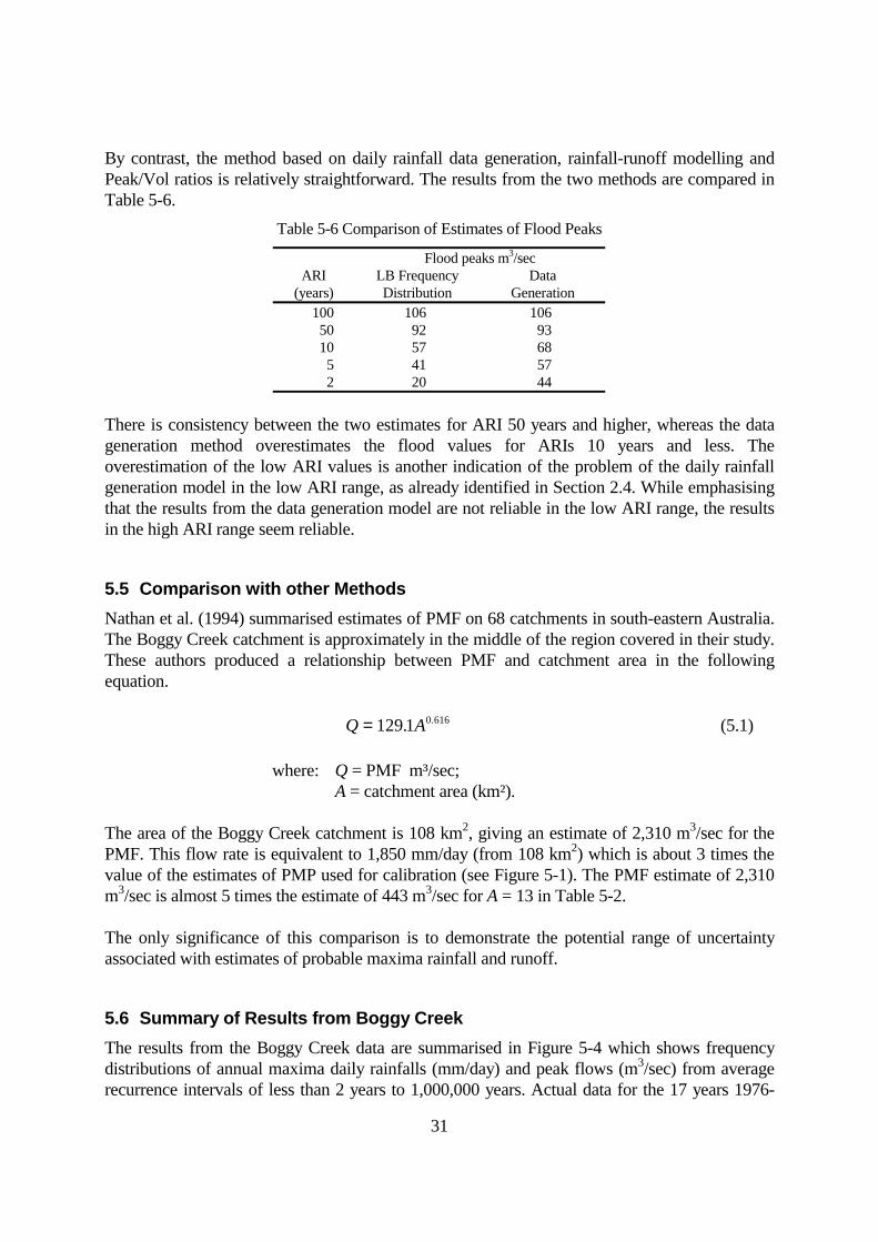
By contrast, the method based on daily rainfall data generation, rainfall-runoff modelling and Peak/Vol ratios is relatively straightforward. The results from the two methods are compared in Table 5-6.

Table 5-6 Comparison of Estimates of Flood Peaks

Flood peaks m3/sec ARI

(years) LB Frequency Distribution

Data Generation

100 106 106 50 92 93 10 57 68 5 41 57 2 20 44

There is consistency between the two estimates for ARI 50 years and higher, whereas the data generation method overestimates the flood values for ARIs 10 years and less. The overestimation of the low ARI values is another indication of the problem of the daily rainfall generation model in the low ARI range, as already identified in Section 2.4. While emphasising that the results from the data generation model are not reliable in the low ARI range, the results in the high ARI range seem reliable.

5.5 Comparison with other Methods Nathan et al. (1994) summarised estimates of PMF on 68 catchments in south-eastern Australia. The Boggy Creek catchment is approximately in the middle of the region covered in their study. These authors produced a relationship between PMF and catchment area in the following equation. Q A= 129 1 0 616. . (5.1) where: Q = PMF m³/sec; A = catchment area (km²). The area of the Boggy Creek catchment is 108 km2, giving an estimate of 2,310 m3/sec for the PMF. This flow rate is equivalent to 1,850 mm/day (from 108 km2) which is about 3 times the value of the estimates of PMP used for calibration (see Figure 5-1). The PMF estimate of 2,310 m3/sec is almost 5 times the estimate of 443 m3/sec for A = 13 in Table 5-2. The only significance of this comparison is to demonstrate the potential range of uncertainty associated with estimates of probable maxima rainfall and runoff.

5.6 Summary of Results from Boggy Creek The results from the Boggy Creek data are summarised in Figure 5-4 which shows frequency distributions of annual maxima daily rainfalls (mm/day) and peak flows (m3/sec) from average recurrence intervals of less than 2 years to 1,000,000 years. Actual data for the 17 years 1976-

32

1992 are shown as solid filled squares and circles and generated data are shown as open squares and circles. The generated daily rainfalls are described in Section 5.1 and are shown in Table 5.1 (A = 13) and the peak flows are described in Section 5.3 and are shown in Table 5.3. Both the generated series of daily rainfalls and peak flows were the results of single runs of length 1,000,000 years. In these runs, there is only one estimate of the 1 in 1,000,000 years value, 10 estimates of the 1 in 100,000 years value, 100 estimates of the 1 in 10,000 years value, and so on. This means the confidence limits are narrower to the left and more open to the right of the generated sequences. Each run of 1,000,000 years takes about 4.5 hours on a 100 megahertz Pentium PC which incorporates a math co-processor and a 16 KB cache memory. Run times will vary depending on the particular PC used for generation. The overall system is a simple and straightforward method for design flood estimation. By comparison, the flood frequency analysis of recorded data gave widely varying answers depending on the inclusion or omission of very low values and/or the length of record available for analysis. The most important result, which can be seen in the "S" shapes of the plots in Figure 5-4, is that no known distribution could reproduce the combination of negative skewness in the low ARI actual data and the positive skewness of the generated values. The data generation system is far more stable than extrapolation from frequency distributions fitted to short periods of data.

10

100

1000

Average Recurrence Interval (years)

106105104103102102 20 505

Generated Daily Rainfall (m m /day)

Actual Daily Rainfall (m m /day)

Actual Peak Flow s (m ³/s)

Generated Peak Flow s (m ³/s)

Figure 5-4 Results from Boggy Creek Catchment

33

6. CONCLUSIONS

6.1 Daily Rainfall Generation Model The daily rainfall generation model uses a transition probability matrix for the direct generation of daily rainfalls less than 15 mm/day and an unbounded frequency distribution for generation of daily rainfalls ≥ 15 mm/day. As Figure 5-4 shows, almost all annual maxima daily rainfalls involved in flood estimation are greater than 15 mm/day. The model seems unreliable for generation of sustained dry periods because it was not possible to generate annual totals of rainfall that were as low as those already recorded in the 58 years of recorded data (see Section 2.4). This does not appear to have any effect on the generated annual maxima daily rainfalls for ARI > 10 years and so does not seem to be a problem when the model is used for flood estimation; however, further testing is required before the model could be used for studies where drought periods are important. The generated annual maxima daily rainfalls for ARI < 10 years should not be used in the flood estimation procedure. The calibration of parameter A in the model is a trial and error procedure with a subjective evaluation against the available calibration data - see Figure 5-1. There are uncertainties in some of the calibration data, such as the CRC-FORGE and PMP estimates, and there are some uncertainties in the generation of low ARI rainfall values. For these reasons, it would be counter-productive to attempt any automatic calibration of A at this time. The subjective calibration is simple and straightforward but somewhat time-consuming.

6.2 Daily Water Balance Rainfall - Runoff Model Although a minor modification was made to the AWBM to make it more flexible for this flood estimation study, the modification proved to make no difference to the results and was unnecessary. The modification was to make the division of generated runoff (storage excess) into surface runoff and baseflow recharge dependent on which surface store generated the runoff. Baseflow recharge was made higher from the smallest surface store, which generates the most runoff events, and lower from the largest surface store, which generates the fewest runoff events. On the Boggy Creek catchment, annual maxima daily runoffs for ARI ≥ about 5 years were all generated from a saturated catchment so that all stores generated the same depth of runoff. The result is that baseflow recharge for ARI ≥ 5 years becomes a fixed fraction of generated storage excess, as in the original AWBM model. The modification proved to be unnecessary, and the calibrated values of the three baseflow recharge fractions were 0.62, 0.60 and 0.62 (see Table 3-3). The more important result from the study is that the constant fraction of generated storage excess going into baseflow recharge (in both the AWBM and DGAWBM models) is the dominating factor determining the annual maxima daily runoff and consequently the annual maxima peak flow. The study of ‘losses’ in Section 3.5 showed that this constant fraction results in an almost constant ratio of annual maxima daily runoff (unrouted surface runoff) to annual maxima daily

34

rainfall (Table 3-5). Because of the large fraction of baseflow in runoff on the Boggy Creek catchment (BFI = 0.6) baseflow recharge virtually determines "loss" in flood estimation on this catchment. It would be easy to assume or guess some function by which baseflow recharge reduced as the magnitude of generated runoff increased; however, such unfounded assumptions hinder rather than help the progress of hydrology. For the present, the importance of baseflow recharge in modelling catchment losses is emphasised as a priority need for further research. The new technique for calibrating the AWBM and DGAWBM models introduced in Section 3.3 was very successful. This uses the output from an established baseflow-surface runoff separation program to calibrate the model such that the correct partition is maintained in monthly totals of flow. It is not an essential part of the flood estimation procedure that this calibration method be used; however, if another method is used, some check should be made to ensure that the generated values of runoff are maintaining proper proportions of baseflow and surface runoff.

6.3 Peak/Volume Ratio The ratio between annual maxima peak flows and annual maxima daily volumes of runoff was established by comparing the frequency distributions of the two variables, as determined from streamflow data. In this study, three methods were tested for comparing the distributions (i) numerical average of the ratios between ranked pairs of values; (ii) linear regression between the ranked pairs of values; and (iii) log-log linear regression between the logarithms of the pairs of values. There was a distinct trend towards a higher peak/vol ratio with increasing ARI, and the log-log regression was selected to produce the results in Section 5.3 because it gives an increasing ratio with increasing ARI, while the other two methods give fixed ratios. The choice of the log-log regression instead of the regression based on natural values gave an increase of about 27% in the ratio at an ARI of 100,000 years but no increase for an ARI of 5 years. The difference between the methods is less than the uncertainties due to the baseflow recharge (see 6.2 above) but is still significant, and it identifies another matter to which some priority of research is warranted.

6.4 Application for Design Flood Estimation This research report has concentrated on demonstrating the potential of using a data generation and a daily water balance model to estimate design peak flows. It has highlighted the urgent need for research into how baseflow recharge varies with event magnitude, particularly for extreme flood events. The method is however directly applicable for use on gauged catchments for routine design flood estimation. Once calibrated, the model can produce estimates of daily runoff for a range of ARIs within a few minutes on a standard PC. This provides an important alternative to event based design flood estimation. Research is continuing on the disaggregation of daily runoff volumes to allow the estimation of design hydrographs at a sub-daily time step.

35

7. REFERENCES Boughton, W. C., 1975 : “A new development in flood frequency estimation”, Hydrology Symposium, I.E.Aust. National Conf. Publ. 75/3. pp 31-35 Boughton, W. C., 1976 : “Flood estimation from short records”, Journal of Hydraulic Engineering, A.S.C.E., v.102, no HY3, pp 241-253. Boughton, W. C., 1980 : “A frequency distribution for annual floods”, Water Resources Research, v.16, no.2, pp.347-354. Boughton, W. C., 1993 : “A hydrograph based model for estimating the water yield of ungauged catchments”, Hydrology & Water Resources Symposium, I. E. Aust., National Conf. Publ. 93/14, pp.319-326. Boughton, W. C., 1996 : “AWBM catchment water balance model, calibration and operation manual, Version 2.0”, unpubl. rept. Boughton, W. C. and Shirley, E. D., 1983 : “Fitting procedures for the log-Boughton distribution”, Journal of Hydraulic Engineering, A.S.C.E., v.109, no.4, pp.579-589. Bradley, A. A., Potter, K. W., 1992 : “Flood frequency analysis of simulated flows”, Water Resources Research, Vol. 28, No. 9, pp 2375-2385. Fuller, W. E., 1914 : “Flood Flows” Trans. of ASCE, Vol. 77., pp.564-617. Haan, C. T., Allen, D. M. and Street, J. D., 1976 : "A Markov chain model of daily rainfall", Water Resources Research, v.12, no.3, pp.443-449. Hill, P. I., 1994 : “Catalogue of hydrologic data for selected Victorian catchments”, Working Document 94/1, CRC for Catchment Hydrology, Monash University, 284 pp. Nandakumar, N., Weinmann, P.E., Mein, R.G., Nathan, R.J., 1997 : Estimation of extreme rainfalls for Victoria using the CRC-FORGE method (for durations 24 to 72 hours). CRC for Catchment Hydrology, Report 97/4, May 1997. Nathan, R. J., Weinmann, P. E. and Gato, S. A., 1994 : “A quick method for estimating the Probable Maximum Flood in south-eastern Australia”, I. E. Aust., National Conf. Publ. 94/15, pp.229-234. Pilgrim D. H. (ed), 1987 : “Australian rainfall and runoff: a guide for flood estimation” Institution of Engineers, Australia. Renard, K. G., Drissel, J. C., Osborn,, H. B., 1970 : “Flood peaks from small south-west range watershed” Journal of Hydraulic Engineering, A.S.C.E., Vol. 96 No. HY3 pp.773-785.

36

Rogers, W. F., 1980 : “A practical model for linear and nonlinear runoff” Journal of Hydrology, Vol. 46 pp51-78. Rogers, W. F., Zia, H. A., 1982 : “Linear and nonlinear runoff from large drainage basins” Journal of Hydrology Vol. 55 pp 267-278. Sharifi, F., 1996 : “Catchment rainfall-runoff computer modelling”, PhD thesis, University of Wollongong, Dept. of Civil and Mining Engineering. Siriwardena, L., Weinmann, P.E., 1996 : “Derivation of Areal Reduction Factors for Design Rainfalls in Victoria for Rainfall Durations 18-120 hours”, CRC for Catchment Hydrology Report 96/4. Srikanthan, R. and McMahon, T. A., 1985 : “Stochastic generation of rainfall and evaporation data”, Australian Water Resources Council, Technical Paper no. 84, 301 pp. Wang, Q.J., 1996a : “The GEV/LH-moment procedure for flood frequency analysis” Advances in Flood Hydrology Workshop course notes, CRC for Catchment Hydrology and IEAust. 30 October 1996. Wang, Q.J. 1996b : “Using higher probability weighted moments for flood frequency analysis” Journal of Hydrology. In press. Watt, W.E., 1971 : “A relationship between peak discharge and maximum twenty-four hour flow for rainfall floods”, Journal of Hydrology, Vol. 14 pp 285-292

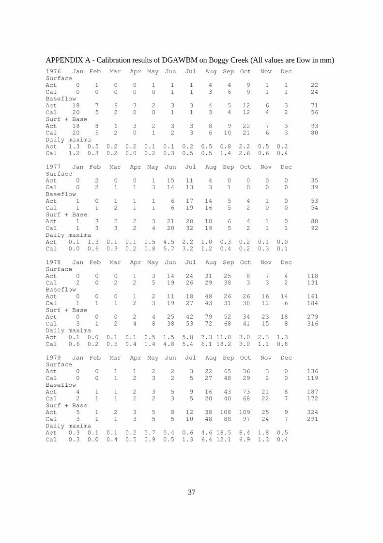
37

APPENDIX A - Calibration results of DGAWBM on Boggy Creek (All values are flow in mm) 1976 Jan Feb Mar Apr May Jun Jul Aug Sep Oct Nov Dec Surface Act 0 1 0 0 1 1 1 4 4 9 1 1 22 Cal 0 0 0 0 0 1 1 3 6 9 1 1 24 Baseflow Act 18 7 6 3 2 3 3 4 5 12 6 3 71 Cal 20 5 2 0 0 1 1 3 4 12 4 2 56 Surf + Base Act 18 8 6 3 2 3 3 8 9 22 7 3 93 Cal 20 5 2 0 1 2 3 6 10 21 6 3 80 Daily maxima Act 1.3 0.5 0.2 0.2 0.1 0.1 0.2 0.5 0.8 2.2 0.5 0.2 Cal 1.2 0.3 0.2 0.0 0.2 0.3 0.5 0.5 1.4 2.6 0.6 0.4 1977 Jan Feb Mar Apr May Jun Jul Aug Sep Oct Nov Dec Surface Act 0 2 0 0 1 15 11 4 0 0 0 0 35 Cal 0 2 1 1 3 14 13 3 1 0 0 0 39 Baseflow Act 1 0 1 1 1 6 17 14 5 4 1 0 53 Cal 1 1 2 1 1 6 19 16 5 2 0 0 54 Surf + Base Act 1 3 2 2 3 21 28 18 6 4 1 0 88 Cal 1 3 3 2 4 20 32 19 5 2 1 1 92 Daily maxima Act 0.1 1.3 0.1 0.1 0.5 4.5 2.2 1.0 0.3 0.2 0.1 0.0 Cal 0.0 0.6 0.3 0.2 0.8 5.7 3.2 1.2 0.4 0.2 0.3 0.1 1978 Jan Feb Mar Apr May Jun Jul Aug Sep Oct Nov Dec Surface Act 0 0 0 1 3 14 24 31 25 8 7 4 118 Cal 2 0 2 2 5 19 26 29 38 3 3 2 131 Baseflow Act 0 0 0 1 2 11 18 48 26 26 16 14 161 Cal 1 1 1 2 3 19 27 43 31 38 12 6 184 Surf + Base Act 0 0 0 2 4 25 42 79 52 34 23 18 279 Cal 3 1 2 4 8 38 53 72 68 41 15 8 316 Daily maxima Act 0.1 0.0 0.1 0.1 0.5 1.5 5.8 7.3 11.0 3.0 2.3 1.3 Cal 0.6 0.2 0.5 0.4 1.4 4.8 5.4 6.1 18.2 3.0 1.1 0.8 1979 Jan Feb Mar Apr May Jun Jul Aug Sep Oct Nov Dec Surface Act 0 0 1 1 2 2 3 22 65 36 3 0 136 Cal 0 0 1 2 3 2 5 27 48 29 2 0 119 Baseflow Act 4 1 1 2 3 5 9 16 43 73 21 8 187 Cal 2 1 1 2 2 3 5 20 40 68 22 7 172 Surf + Base Act 5 1 2 3 5 8 12 38 108 109 25 9 324 Cal 3 1 1 3 5 5 10 48 88 97 24 7 291 Daily maxima Act 0.3 0.1 0.1 0.2 0.7 0.4 0.6 4.6 18.5 8.4 1.8 0.5 Cal 0.3 0.0 0.4 0.5 0.9 0.5 1.3 6.4 12.1 6.9 1.3 0.4

38

1980 Jan Feb Mar Apr May Jun Jul Aug Sep Oct Nov Dec Surface Act 1 0 1 1 3 3 31 22 11 2 1 3 78 Cal 1 0 1 3 2 9 32 23 15 2 0 3 92 Baseflow Act 3 1 1 1 2 3 17 42 34 24 9 5 143 Cal 2 1 1 1 3 3 28 42 27 15 4 3 130 Surf + Base Act 4 1 2 1 5 7 48 64 45 26 10 9 221 Cal 4 1 2 4 5 11 60 65 42 17 5 7 222 Daily maxima Act 0.5 0.1 0.1 0.3 0.3 1.5 7.8 4.3 3.1 1.5 0.7 1.0 Cal 0.7 0.0 0.4 1.3 0.9 4.6 7.9 6.7 6.7 0.9 0.3 1.0 1981 Jan Feb Mar Apr May Jun Jul Aug Sep Oct Nov Dec Surface Act 1 1 0 0 1 48 113 53 4 5 2 1 228 Cal 2 1 1 0 3 43 102 81 3 3 1 1 240 Baseflow Act 1 1 1 1 1 11 81 144 53 25 13 6 338 Cal 2 2 2 1 1 20 92 141 62 21 6 2 352 Surf + Base Act 2 2 2 1 1 58 194 197 57 30 15 7 567 Cal 4 3 2 1 4 63 193 222 65 25 7 3 592 Daily maxima Act 0.3 0.1 0.1 0.2 0.1 15.7 28.3 11.4 3.7 2.0 0.9 0.6 Cal 1.0 0.4 0.4 0.1 0.4 9.2 21.7 13.2 4.3 2.8 0.5 0.5 1982 Jan Feb Mar Apr May Jun Jul Aug Sep Oct Nov Dec Surface Act 1 0 1 1 1 1 2 0 0 0 0 0 7 Cal 1 0 1 1 2 2 0 0 1 0 0 0 9 Baseflow Act 2 1 1 0 1 2 3 2 1 1 0 0 14 Cal 1 1 1 1 1 2 1 1 1 1 0 0 11 Surf + Base Act 3 1 2 1 2 3 5 2 1 1 0 0 21 Cal 2 1 2 2 3 4 2 1 2 1 0 1 21 Daily maxima Act 0.2 0.1 0.1 0.1 0.1 0.1 0.2 0.2 0.2 0.0 0.0 0.0 Cal 0.7 0.1 0.4 0.4 0.5 0.3 0.2 0.2 0.6 0.1 0.0 0.3 1983 Jan Feb Mar Apr May Jun Jul Aug Sep Oct Nov Dec Surface Act 0 0 0 3 9 7 35 34 47 4 2 2 144 Cal 0 0 4 4 22 14 43 42 47 2 1 1 179 Baseflow Act 0 0 0 1 7 13 29 50 65 39 16 11 232 Cal 0 0 2 4 17 22 32 60 72 36 10 4 259 Surf + Base Act 0 0 1 4 17 20 64 84 112 43 18 14 376 Cal 0 0 6 8 39 36 75 102 118 38 10 5 438 Daily maxima Act 0.0 0.0 0.3 1.5 1.2 1.6 7.1 7.3 9.1 2.9 0.8 1.4 Cal 0.0 0.2 1.8 1.0 4.7 3.4 10.7 12.9 9.9 2.7 0.5 0.5

39

1984 Jan Feb Mar Apr May Jun Jul Aug Sep Oct Nov Dec Surface Act 15 0 1 1 0 1 4 58 15 25 0 0 120 Cal 6 0 1 1 0 1 3 34 11 11 0 0 69 Baseflow Act 11 8 5 5 3 2 4 25 42 40 11 4 161 Cal 5 2 1 1 1 1 2 21 29 24 6 2 96 Surf + Base Act 26 9 6 6 3 3 8 83 57 65 11 4 281 Cal 11 3 3 2 1 2 5 55 40 35 6 2 166 Daily maxima Act 4.3 0.6 0.3 0.3 0.2 0.2 0.6 14.5 5.7 15.7 0.8 0.2 Cal 1.6 0.3 0.4 0.3 0.2 0.4 0.6 7.2 4.9 6.1 0.4 0.1 1985 Jan Feb Mar Apr May Jun Jul Aug Sep Oct Nov Dec Surface Act 0 0 0 1 3 2 3 42 2 3 1 6 63 Cal 0 0 1 2 3 3 6 40 1 2 1 2 60 Baseflow Act 2 1 0 0 1 4 5 24 25 10 7 9 89 Cal 0 0 1 2 1 4 5 32 23 7 3 3 82 Surf + Base Act 2 1 0 1 4 6 8 65 28 13 9 15 152 Cal 1 0 2 3 4 7 11 72 24 9 4 5 142 Daily maxima Act 0.1 0.1 0.0 0.1 0.9 0.6 0.5 5.7 2.3 1.1 0.5 2.0 Cal 0.1 0.1 0.5 0.5 1.1 0.6 1.5 6.1 1.5 0.5 0.5 0.7 1986 Jan Feb Mar Apr May Jun Jul Aug Sep Oct Nov Dec Surface Act 0 0 0 1 9 1 90 22 19 27 1 3 173 Cal 0 1 0 3 10 5 80 23 18 25 0 2 166 Baseflow Act 4 1 1 0 3 8 61 46 37 45 34 13 252 Cal 1 1 0 1 6 9 69 58 36 29 22 7 239 Surf + Base Act 4 1 1 1 12 9 151 67 56 72 35 16 425 Cal 1 1 0 4 16 14 149 81 54 53 22 9 405 Daily maxima Act 0.2 0.1 0.0 0.2 2.2 0.4 12.7 6.9 6.8 6.2 2.5 1.5 Cal 0.1 0.4 0.0 0.8 4.2 1.3 12.0 9.8 9.0 10.3 1.3 0.9 1987 Jan Feb Mar Apr May Jun Jul Aug Sep Oct Nov Dec Surface Act 1 1 1 1 2 41 29 15 2 3 1 1 97 Cal 0 2 0 2 3 21 20 10 1 1 1 1 61 Baseflow Act 5 1 2 2 2 13 31 44 25 10 5 3 144 Cal 2 1 1 1 3 11 27 25 10 4 1 1 88 Surf + Base Act 6 2 3 3 4 53 61 59 26 13 6 4 240 Cal 2 3 2 3 6 32 47 35 11 5 2 2 149 Daily maxima Act 0.3 0.4 0.1 0.2 0.2 12.1 5.8 4.2 1.4 0.7 0.3 0.6 Cal 0.1 1.0 0.2 0.6 0.8 6.0 5.1 2.7 0.7 0.5 0.2 0.4

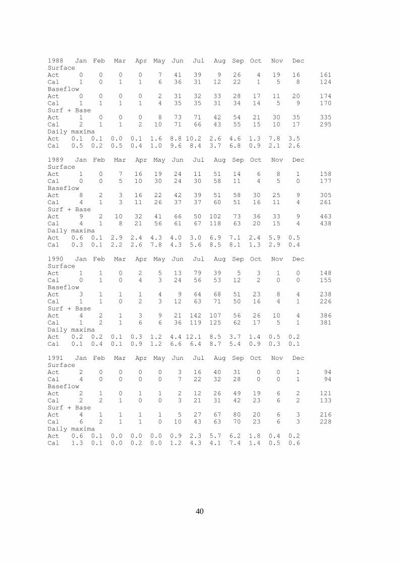
40

1988 Jan Feb Mar Apr May Jun Jul Aug Sep Oct Nov Dec Surface Act 0 0 0 0 7 41 39 9 26 4 19 16 161 Cal 1 0 1 1 6 36 31 12 22 1 5 8 124 Baseflow Act 0 0 0 0 2 31 32 33 28 17 11 20 174 Cal 1 1 1 1 4 35 35 31 34 14 5 9 170 Surf + Base Act 1 0 0 0 8 73 71 42 54 21 30 35 335 Cal 2 1 1 2 10 71 66 43 55 15 10 17 295 Daily maxima Act 0.1 0.1 0.0 0.1 1.6 8.8 10.2 2.6 4.6 1.3 7.8 3.5 Cal 0.5 0.2 0.5 0.4 1.0 9.6 8.4 3.7 6.8 0.9 2.1 2.6 1989 Jan Feb Mar Apr May Jun Jul Aug Sep Oct Nov Dec Surface Act 1 0 7 16 19 24 11 51 14 6 8 1 158 Cal 0 0 5 10 30 24 30 58 11 4 5 0 177 Baseflow Act 8 2 3 16 22 42 39 51 58 30 25 9 305 Cal 4 1 3 11 26 37 37 60 51 16 11 4 261 Surf + Base Act 9 2 10 32 41 66 50 102 73 36 33 9 463 Cal 4 1 8 21 56 61 67 118 63 20 15 4 438 Daily maxima Act 0.6 0.1 2.9 2.4 4.3 4.0 3.0 6.9 7.1 2.4 5.9 0.5 Cal 0.3 0.1 2.2 2.6 7.8 4.3 5.6 8.5 8.1 1.3 2.9 0.4 1990 Jan Feb Mar Apr May Jun Jul Aug Sep Oct Nov Dec Surface Act 1 1 0 2 5 13 79 39 5 3 1 0 148 Cal 0 1 0 4 3 24 56 53 12 2 0 0 155 Baseflow Act 3 1 1 1 4 9 64 68 51 23 8 4 238 Cal 1 1 0 2 3 12 63 71 50 16 4 1 226 Surf + Base Act 4 2 1 3 9 21 142 107 56 26 10 4 386 Cal 1 2 1 6 6 36 119 125 62 17 5 1 381 Daily maxima Act 0.2 0.2 0.1 0.3 1.2 4.4 12.1 8.5 3.7 1.4 0.5 0.2 Cal 0.1 0.4 0.1 0.9 1.2 6.6 6.4 8.7 5.4 0.9 0.3 0.1 1991 Jan Feb Mar Apr May Jun Jul Aug Sep Oct Nov Dec Surface Act 2 0 0 0 0 3 16 40 31 0 0 1 94 Cal 4 0 0 0 0 7 22 32 28 0 0 1 94 Baseflow Act 2 1 0 1 1 2 12 26 49 19 6 2 121 Cal 2 2 1 0 0 3 21 31 42 23 6 2 133 Surf + Base Act 4 1 1 1 1 5 27 67 80 20 6 3 216 Cal 6 2 1 1 0 10 43 63 70 23 6 3 228 Daily maxima Act 0.6 0.1 0.0 0.0 0.0 0.9 2.3 5.7 6.2 1.8 0.4 0.2 Cal 1.3 0.1 0.0 0.2 0.0 1.2 4.3 4.1 7.4 1.4 0.5 0.6

41

1992 Jan Feb Mar Apr May Jun Jul Aug Sep Oct Nov Dec Surface Act 1 0 1 1 12 7 8 33 55 22 20 9 169 Cal 1 0 2 2 11 11 14 34 55 30 8 4 172 Baseflow Act 1 0 1 1 6 13 18 35 73 74 31 34 287 Cal 2 1 2 1 8 14 17 30 61 65 28 14 243 Surf + Base Act 2 1 1 2 18 20 26 68 128 97 51 43 456 Cal 3 1 4 3 19 26 31 64 116 95 36 18 416 Daily maxima Act 0.4 0.0 0.3 0.2 2.3 1.2 2.1 6.5 8.8 8.3 6.9 3.9 Cal 0.8 0.1 0.8 0.5 3.3 2.6 3.0 7.7 9.9 8.9 3.5 1.4

The Cooperative Research Centre for Catchment Hydrology is a cooperative venture formed under the Commonwealth CRC Program between:

Bureau of Meteorology CSIRO Land and Water

Department of Natural Resources and Environment, Vic Goulburn-Murray Water

Melbourne Water Monash University

Murray-Darling Basin Commission Southern Rural Water

The University of Melbourne Wimmera-Mallee Water

Associates

Department of Land and Water Conservation, NSW Department of Natural Resources, Qld

Hydro-Electric Corporation, Tas State Forests of NSW

Centre Office Department of Civil Engineering, PO Box 60 Monash University, Victoria, 3800, Australia. Telephone: (03) 9905 2704 Facsimile: (03) 9905 5033 International +61 3 9905 2704

http://www.catchment.crc.org.au