A Description of the Advanced Research WRF Version 3 · A Description of the Advanced Research WRF...

NCAR/TN–475+STRNCAR TECHNICAL NOTE

June 2008

A Description of theAdvanced Research WRF Version 3

William C. SkamarockJoseph B. KlempJimy DudhiaDavid O. GillDale M. BarkerMichael G. DudaXiang-Yu HuangWei WangJordan G. Powers

Mesoscale and Microscale Meteorology DivisionNational Center for Atmospheric Research

Boulder, Colorado, USA

NCAR TECHNICAL NOTES

The Technical Note series provides an outlet for a variety of NCAR manuscripts that contributein specialized ways to the body of scientific knowledge but which are not suitable for journal,monograph, or book publication. Reports in this series are issued by the NCAR Scientific Di-visions; copies may be obtained on request from the Publications Office of NCAR. Designationsymbols for the series include:

EDD: Engineering, Design, or Development ReportsEquipment descriptions, test results, instrumentation,and operating and maintenance manuals.

IA: Instructional AidsInstruction manuals, bibliographies, film supplements,and other research or instructional aids.

PPR: Program Progress ReportsField program reports, interim and working reports,survey reports, and plans for experiments.

PROC: ProceedingsDocumentation of symposia, colloquia, conferences, workshops,and lectures. (Distribution may be limited to attendees.)

STR: Scientific and Technical ReportsData compilations, theoretical and numericalinvestigations, and experimental results.

The National Center for Atmospheric Research (NCAR) is operated by the University Corpora-tion for Atmospheric Research (UCAR) and is sponsored by the National Science Foundation.Any opinions, findings, conclusions, or recommendations expressed in this publication are thoseof the authors and do not necessarily reflect the views of the National Science Foundation.

Contents

Acknowledgments ix

1 Introduction 11.1 Advanced Research WRF . . . . . . . . . . . . . . . . . . . . . . . . . . . . . . 21.2 Major Features of the ARW System, Version 3 . . . . . . . . . . . . . . . . . . . 3

2 Governing Equations 72.1 Vertical Coordinate and Variables . . . . . . . . . . . . . . . . . . . . . . . . . . 72.2 Flux-Form Euler Equations . . . . . . . . . . . . . . . . . . . . . . . . . . . . . 82.3 Inclusion of Moisture . . . . . . . . . . . . . . . . . . . . . . . . . . . . . . . . . 92.4 Map Projections, Coriolis and Curvature Terms . . . . . . . . . . . . . . . . . . 92.5 Perturbation Form of the Governing Equations . . . . . . . . . . . . . . . . . . . 11

3 Model Discretization 133.1 Temporal Discretization . . . . . . . . . . . . . . . . . . . . . . . . . . . . . . . 13

3.1.1 Runge-Kutta Time Integration Scheme . . . . . . . . . . . . . . . . . . . 133.1.2 Acoustic Integration . . . . . . . . . . . . . . . . . . . . . . . . . . . . . 143.1.3 Full Time-Split Integration Sequence . . . . . . . . . . . . . . . . . . . . 173.1.4 Diabatic Forcing . . . . . . . . . . . . . . . . . . . . . . . . . . . . . . . 173.1.5 Hydrostatic Option . . . . . . . . . . . . . . . . . . . . . . . . . . . . . . 18

3.2 Spatial Discretization . . . . . . . . . . . . . . . . . . . . . . . . . . . . . . . . . 183.2.1 Acoustic Step Equations . . . . . . . . . . . . . . . . . . . . . . . . . . . 183.2.2 Coriolis and Curvature Terms . . . . . . . . . . . . . . . . . . . . . . . . 203.2.3 Advection . . . . . . . . . . . . . . . . . . . . . . . . . . . . . . . . . . . 213.2.4 Pole Conditions for the Global Latitude-Longitude Grid . . . . . . . . . 24

3.3 Stability Constraints . . . . . . . . . . . . . . . . . . . . . . . . . . . . . . . . . 243.3.1 RK3 Time Step Constraint . . . . . . . . . . . . . . . . . . . . . . . . . . 253.3.2 Acoustic Time Step Constraint . . . . . . . . . . . . . . . . . . . . . . . 253.3.3 Adaptive Time Step . . . . . . . . . . . . . . . . . . . . . . . . . . . . . 263.3.4 Map Projection Considerations . . . . . . . . . . . . . . . . . . . . . . . 27

4 Turbulent Mixing and Model Filters 294.1 Latitude-Longitude Global Grid and Polar Filtering . . . . . . . . . . . . . . . . 294.2 Explicit Spatial Diffusion . . . . . . . . . . . . . . . . . . . . . . . . . . . . . . . 30

4.2.1 Horizontal and Vertical Diffusion on Coordinate Surfaces . . . . . . . . . 304.2.2 Horizontal and Vertical Diffusion in Physical Space . . . . . . . . . . . . 31

i

4.2.3 Computation of the Eddy Viscosities . . . . . . . . . . . . . . . . . . . . 334.2.4 TKE equation for the 1.5 Order Turbulence Closure . . . . . . . . . . . . 344.2.5 Sixth-Order Spatial Filter on Coordinate Surfaces . . . . . . . . . . . . . 35

4.3 Filters for the Time-split RK3 scheme . . . . . . . . . . . . . . . . . . . . . . . . 364.3.1 Three-Dimensional Divergence Damping . . . . . . . . . . . . . . . . . . 364.3.2 External Mode Filter . . . . . . . . . . . . . . . . . . . . . . . . . . . . . 364.3.3 Semi-Implicit Acoustic Step Off-centering . . . . . . . . . . . . . . . . . . 37

4.4 Formulations for Gravity Wave Absorbing Layers . . . . . . . . . . . . . . . . . 374.4.1 Absorbing Layer Using Spatial Filtering . . . . . . . . . . . . . . . . . . 374.4.2 Implicit Rayleigh Damping for the Vertical Velocity . . . . . . . . . . . . 374.4.3 Traditional Rayleigh Damping Layer . . . . . . . . . . . . . . . . . . . . 38

4.5 Other Damping . . . . . . . . . . . . . . . . . . . . . . . . . . . . . . . . . . . . 394.5.1 Vertical-Velocity Damping . . . . . . . . . . . . . . . . . . . . . . . . . . 39

5 Initial Conditions 415.1 Initialization for Idealized Conditions . . . . . . . . . . . . . . . . . . . . . . . . 415.2 Initialization for Real-Data Conditions . . . . . . . . . . . . . . . . . . . . . . . 43

5.2.1 Use of the WRF Preprocessing System by the ARW . . . . . . . . . . . . 435.2.2 Reference State . . . . . . . . . . . . . . . . . . . . . . . . . . . . . . . . 435.2.3 Vertical Interpolation and Extrapolation . . . . . . . . . . . . . . . . . . 455.2.4 Perturbation State . . . . . . . . . . . . . . . . . . . . . . . . . . . . . . 455.2.5 Generating Lateral Boundary Data . . . . . . . . . . . . . . . . . . . . . 465.2.6 Masking of Surface Fields . . . . . . . . . . . . . . . . . . . . . . . . . . 47

5.3 Digital Filtering Initialization . . . . . . . . . . . . . . . . . . . . . . . . . . . . 475.3.1 Filter Design . . . . . . . . . . . . . . . . . . . . . . . . . . . . . . . . . 485.3.2 DFI Schemes . . . . . . . . . . . . . . . . . . . . . . . . . . . . . . . . . 485.3.3 Backward Integration . . . . . . . . . . . . . . . . . . . . . . . . . . . . . 50

6 Lateral Boundary Conditions 516.1 Periodic Lateral Boundary Conditions . . . . . . . . . . . . . . . . . . . . . . . 516.2 Open Lateral Boundary Conditions . . . . . . . . . . . . . . . . . . . . . . . . . 516.3 Symmetric Lateral Boundary Conditions . . . . . . . . . . . . . . . . . . . . . . 526.4 Specified Lateral Boundary Conditions . . . . . . . . . . . . . . . . . . . . . . . 526.5 Polar Conditions . . . . . . . . . . . . . . . . . . . . . . . . . . . . . . . . . . . 54

7 Nesting 557.1 Nesting Options . . . . . . . . . . . . . . . . . . . . . . . . . . . . . . . . . . . . 557.2 Staggering and Feedback . . . . . . . . . . . . . . . . . . . . . . . . . . . . . . . 587.3 Nested Lateral Boundary Conditions . . . . . . . . . . . . . . . . . . . . . . . . 607.4 Steps to Generate a Nest Grid . . . . . . . . . . . . . . . . . . . . . . . . . . . . 61

8 Physics 658.1 Microphysics . . . . . . . . . . . . . . . . . . . . . . . . . . . . . . . . . . . . . . 65

8.1.1 Kessler scheme . . . . . . . . . . . . . . . . . . . . . . . . . . . . . . . . 668.1.2 Purdue Lin scheme . . . . . . . . . . . . . . . . . . . . . . . . . . . . . . 678.1.3 WRF Single-Moment 3-class (WSM3) scheme . . . . . . . . . . . . . . . 67

ii

8.1.4 WSM5 scheme . . . . . . . . . . . . . . . . . . . . . . . . . . . . . . . . 678.1.5 WSM6 scheme . . . . . . . . . . . . . . . . . . . . . . . . . . . . . . . . 678.1.6 Eta Grid-scale Cloud and Precipitation (2001) scheme . . . . . . . . . . . 688.1.7 Thompson et al. scheme . . . . . . . . . . . . . . . . . . . . . . . . . . . 688.1.8 Goddard Cumulus Ensemble Model scheme . . . . . . . . . . . . . . . . 698.1.9 Morrison et al. 2-Moment scheme . . . . . . . . . . . . . . . . . . . . . . 69

8.2 Cumulus parameterization . . . . . . . . . . . . . . . . . . . . . . . . . . . . . . 708.2.1 Kain-Fritsch scheme . . . . . . . . . . . . . . . . . . . . . . . . . . . . . 708.2.2 Betts-Miller-Janjic scheme . . . . . . . . . . . . . . . . . . . . . . . . . . 718.2.3 Grell-Devenyi ensemble scheme . . . . . . . . . . . . . . . . . . . . . . . 718.2.4 Grell-3 scheme . . . . . . . . . . . . . . . . . . . . . . . . . . . . . . . . 72

8.3 Surface Layer . . . . . . . . . . . . . . . . . . . . . . . . . . . . . . . . . . . . . 728.3.1 Similarity theory (MM5) . . . . . . . . . . . . . . . . . . . . . . . . . . . 728.3.2 Similarity theory (Eta) . . . . . . . . . . . . . . . . . . . . . . . . . . . . 728.3.3 Similarity theory (PX) . . . . . . . . . . . . . . . . . . . . . . . . . . . . 73

8.4 Land-Surface Model . . . . . . . . . . . . . . . . . . . . . . . . . . . . . . . . . 738.4.1 5-layer thermal diffusion . . . . . . . . . . . . . . . . . . . . . . . . . . . 738.4.2 Noah LSM . . . . . . . . . . . . . . . . . . . . . . . . . . . . . . . . . . . 738.4.3 Rapid Update Cycle (RUC) Model LSM . . . . . . . . . . . . . . . . . . 748.4.4 Pleim-Xiu LSM . . . . . . . . . . . . . . . . . . . . . . . . . . . . . . . . 758.4.5 Urban Canopy Model . . . . . . . . . . . . . . . . . . . . . . . . . . . . . 758.4.6 Ocean Mixed-Layer Model . . . . . . . . . . . . . . . . . . . . . . . . . . 758.4.7 Specified Lower Boundary Conditions . . . . . . . . . . . . . . . . . . . . 76

8.5 Planetary Boundary Layer . . . . . . . . . . . . . . . . . . . . . . . . . . . . . . 768.5.1 Medium Range Forecast Model (MRF) PBL . . . . . . . . . . . . . . . . 768.5.2 Yonsei University (YSU) PBL . . . . . . . . . . . . . . . . . . . . . . . . 778.5.3 Mellor-Yamada-Janjic (MYJ) PBL . . . . . . . . . . . . . . . . . . . . . 778.5.4 Asymmetrical Convective Model version 2 (ACM2) PBL . . . . . . . . . 78

8.6 Atmospheric Radiation . . . . . . . . . . . . . . . . . . . . . . . . . . . . . . . . 788.6.1 Rapid Radiative Transfer Model (RRTM) Longwave . . . . . . . . . . . . 788.6.2 Eta Geophysical Fluid Dynamics Laboratory (GFDL) Longwave . . . . . 798.6.3 CAM Longwave . . . . . . . . . . . . . . . . . . . . . . . . . . . . . . . . 798.6.4 Eta Geophysical Fluid Dynamics Laboratory (GFDL) Shortwave . . . . . 798.6.5 MM5 (Dudhia) Shortwave . . . . . . . . . . . . . . . . . . . . . . . . . . 808.6.6 Goddard Shortwave . . . . . . . . . . . . . . . . . . . . . . . . . . . . . . 808.6.7 CAM Shortwave . . . . . . . . . . . . . . . . . . . . . . . . . . . . . . . 80

8.7 Physics Interactions . . . . . . . . . . . . . . . . . . . . . . . . . . . . . . . . . . 808.8 Four-Dimensional Data Assimilation . . . . . . . . . . . . . . . . . . . . . . . . 82

8.8.1 Grid Nudging or Analysis Nudging . . . . . . . . . . . . . . . . . . . . . 828.8.2 Observational or Station Nudging . . . . . . . . . . . . . . . . . . . . . . 83

9 Variational Data Assimilation 879.1 Introduction . . . . . . . . . . . . . . . . . . . . . . . . . . . . . . . . . . . . . . 879.2 Improvements to the WRF-Var Algorithm . . . . . . . . . . . . . . . . . . . . . 89

9.2.1 Improved vertical interpolation . . . . . . . . . . . . . . . . . . . . . . . 89

iii

9.2.2 Improved minimization and “outer loop” . . . . . . . . . . . . . . . . . . 899.2.3 Choice of control variables . . . . . . . . . . . . . . . . . . . . . . . . . . 909.2.4 First Guess at Appropriate Time (FGAT) . . . . . . . . . . . . . . . . . 909.2.5 Radar Data Assimilation . . . . . . . . . . . . . . . . . . . . . . . . . . . 909.2.6 Unified Regional/Global 3D-Var Assimilation . . . . . . . . . . . . . . . 91

9.3 Background Error Covariances . . . . . . . . . . . . . . . . . . . . . . . . . . . . 929.3.1 Removal of time-mean . . . . . . . . . . . . . . . . . . . . . . . . . . . . 949.3.2 Multivariate Covariances: Regression coefficients and unbalanced variables 949.3.3 Vertical Covariances: Eigenvectors/eigenvalues and control variable pro-

jections . . . . . . . . . . . . . . . . . . . . . . . . . . . . . . . . . . . . 959.3.4 Horizontal Covariances: Recursive filter lengthscale (regional), or power

spectra (global) . . . . . . . . . . . . . . . . . . . . . . . . . . . . . . . . 959.4 WRF-Var V3.0 Software Engineering Improvements . . . . . . . . . . . . . . . . 95

9.4.1 Memory improvements . . . . . . . . . . . . . . . . . . . . . . . . . . . . 959.4.2 Four-Byte I/O . . . . . . . . . . . . . . . . . . . . . . . . . . . . . . . . . 969.4.3 Switch from RSL to RSL LITE . . . . . . . . . . . . . . . . . . . . . . . 969.4.4 Reorganisation of observation structures . . . . . . . . . . . . . . . . . . 969.4.5 Radar reflectivity operators redesigned . . . . . . . . . . . . . . . . . . . 96

Appendices

A Physical Constants 97

B List of Symbols 99

C Acronyms 103

References 105

iv

List of Figures

1.1 WRF system components. . . . . . . . . . . . . . . . . . . . . . . . . . . . . . . 2

2.1 ARW η coordinate. . . . . . . . . . . . . . . . . . . . . . . . . . . . . . . . . . . 7

3.1 Time step integration sequence. Here n represents the number of acoustic timesteps for a given substep of the RK3 integration, and ns is the ratio of the RK3time step to the acoustic time step for the second and third RK3 substeps. . . . 16

3.2 Horizontal and vertical grids of the ARW . . . . . . . . . . . . . . . . . . . . . . 193.3 Latitude-longitude grid structure in the pole region. In the ARW formulation,

re∆ψ = ∆y/my. . . . . . . . . . . . . . . . . . . . . . . . . . . . . . . . . . . . . 24

5.1 Schematic showing the data flow and program components in WPS, and how WPSfeeds initial data to the ARW. Letters in the rectangular boxes indicate programnames. GEOGRID: defines the model domain and creates static files of terrestrialdata. UNGRIB: decodes GriB data. METGRID: interpolates meteorological datato the model domain. . . . . . . . . . . . . . . . . . . . . . . . . . . . . . . . . . 44

5.2 An illustration showing the three available DFI schemes: digital filter launch,diabatic digital filter initialization, and twice digital filter initialization. . . . . . 49

6.1 Specified and relaxation zones for a grid with a single specified row and column,and four rows and columns for the relaxation zone. These are typical values usedfor a specified lateral boundary condition for a real-data case. . . . . . . . . . . 53

7.1 1-way and 2-way nesting options in the ARW. . . . . . . . . . . . . . . . . . . . 567.2 Various nest configurations for multiple grids. (a) Telescoping nests. (b) Nests at

the same level with respect to a parent grid. (c) Overlapping grids: not allowed(d) Inner-most grid has more than one parent grid: not allowed . . . . . . . . . 57

7.3 Arakawa-C grid staggering for a portion of a parent domain and an imbeddednest domain with a 3:1 grid size ratio. The solid lines denote coarse grid cellboundaries, and the dashed lines are the boundaries for each fine grid cell. Thehorizontal components of velocity (“U” and “V”) are defined along the normal cellface, and the thermodynamic variables (“θ”) are defined at the center of the gridcell (each square). The bold typeface variables along the interface between thecoarse and the fine grid define the locations where the specified lateral boundariesfor the nest are in effect. . . . . . . . . . . . . . . . . . . . . . . . . . . . . . . 59

7.4 Similar to Fig. 7.3, but with a 2:1 grid-distance ratio. . . . . . . . . . . . . . . 617.5 Nest grid integration sequence. . . . . . . . . . . . . . . . . . . . . . . . . . . . . 62

v

7.6 Zones of topographic blending for a fine grid. In the fine grid, the first zone isentirely interpolated from the coarse grid topography. In the second zone, thetopography is linearly weighted between the coarse grid and the fine grid. . . . . 63

9.1 Sketch showing the relationship between datasets (circles), and algorithms (rect-angles) of the ARW system. . . . . . . . . . . . . . . . . . . . . . . . . . . . . . 88

9.2 Sketch of the role of Stage 0 converters in transforming model-specific data (e.g.,ARW, KMA global model, etc.) to standard perturbation fields and relevantmetadata (e.g., latitude, height, land/sea, etc.). . . . . . . . . . . . . . . . . . . 93

vi

List of Tables

3.1 Maximum stable Courant numbers for one-dimensional linear advection. FromWicker and Skamarock (2002). . . . . . . . . . . . . . . . . . . . . . . . . . . . . 25

8.1 Microphysics Options . . . . . . . . . . . . . . . . . . . . . . . . . . . . . . . . . 668.2 Cumulus Parameterization Options . . . . . . . . . . . . . . . . . . . . . . . . . 708.3 Land Surface Options . . . . . . . . . . . . . . . . . . . . . . . . . . . . . . . . . 748.4 Planetary Boundary Layer Options . . . . . . . . . . . . . . . . . . . . . . . . . 778.5 Radiation Options . . . . . . . . . . . . . . . . . . . . . . . . . . . . . . . . . . 798.6 Physics Interactions. Columns correspond to model physical processes: radiation

(Rad), microphysics (MP), cumulus parameterization (CP), planetary boundarylayer/vertical diffusion (PBL), and surface physics (Sfc). Rows corresponds tomodel variables where i and o indicate whether a variable is input or output(updated) by a physical process. . . . . . . . . . . . . . . . . . . . . . . . . . . . 81

vii

Acknowledgments

Many people beyond this document’s author list have contributed to the development of dy-namics and physics. For the dynamics solver development, we would like to thank Louis Wickerfor his assistance with the Runge-Kutta integration scheme; George Bryan and Jason Knievelfor contributing in the turbulent mixing algorithms and other model filters; Mark Richardson,Anthony Toigo and Claire Newman for generalizing the WRF code for global applications.

For physics contributions, we would like to thank Tom Black, John Brown, Kenneth Cam-pana, Fei Chen, Shu-Hua Chen, Ming-Da Chou, Aijun Deng, Mike Ek, Brad Ferrier, Georg Grell,Bill Hall, Songyou Hong, Zavisa Janjic, Jack Kain, Hiroyuki Kusaka, Ruby Leung, Jeong-OckLim, Kyo-Sun Lim, Yubao Liu, Chin-Hoh Moeng, Ken Mitchell, Eli Mlawer, Hugh Morrison, JonPleim, Tanya Smirnova, Dave Stauffer, Wei-Kuo Tao, Mukul Tewari, Greg Thompson, GuentherZaengl and others. We also acknowledge the contribution by Min Chen, Ju-Won Kim, StevenPeckham, Tanya Smirnova, John Brown and Stan Benjamin for the digital filter initializationdevelopment.

The development of WRF-Var represents an international team effort. We would like toacknowledge the following people for their contributions to the WRF-Var system: Yong-RunGuo, Wei Huang, Qingnong Xiao, Syed Rizvi, Francois Vandenberghe, Mike McAtee, Roy Peck,Wan-Shu Wu, Dezso Devenyi, Jianfeng Gu, Mi-Seon Lee, Ki-Han Youn, Eunha Lim, Hyun-Cheol Shin, Shu-Hua Chen, Hui-Chuan Lin, John Bray, Xin Zhang, Zhiquan Liu, Tom Auligne,Xianyan Zhang, and Yongsheng Chen.

We would like express our appreciation to John Michalakes for developing the WRF SoftwareFramework. We would also like thank Jacques Middlecoff, Tom Henderson, Al Bourgeois, MattBettencourt, Todd Hutchinson, Kent Yang, and Dan Schaffer for their contributions to thesoftware development.

Finally, we would like to thank George Bryan, Jim Bresch, Jian-Wen Bao and John Brownfor their careful review of this document. We also thank Cindy Bruyere for assistance with thegraphics.

The Weather Research and Forecasting model effort is supported by the National ScienceFoundation, the Department of Defense, the National Oceanic and Atmospheric Administration,and the Federal Aviation Administration.

ix

Chapter 1

Introduction

The Weather Research and Forecasting (WRF) model is a numerical weather prediction (NWP)and atmospheric simulation system designed for both research and operational applications.WRF is supported as a common tool for the university/research and operational communitiesto promote closer ties between them and to address the needs of both. The development ofWRF has been a multi-agency effort to build a next-generation mesoscale forecast model anddata assimilation system to advance the understanding and prediction of mesoscale weather andaccelerate the transfer of research advances into operations. The WRF effort has been a collab-orative one among the National Center for Atmospheric Research’s (NCAR) Mesoscale and Mi-croscale Meteorology (MMM) Division, the National Oceanic and Atmospheric Administration’s(NOAA) National Centers for Environmental Prediction (NCEP) and Earth System ResearchLaboratory (ESRL), the Department of Defense’s Air Force Weather Agency (AFWA) and NavalResearch Laboratory (NRL), the Center for Analysis and Prediction of Storms (CAPS) at theUniversity of Oklahoma, and the Federal Aviation Administration (FAA), with the participationof university scientists.

WRF reflects flexible, state-of-the-art, portable code that is efficient in computing environ-ments ranging from massively-parallel supercomputers to laptops. Its modular, single-sourcecode can be configured for both research and operational applications. Its spectrum of physicsand dynamics options reflects the experience and input of the broad scientific community. ItsWRF-Var variational data assimilation system can ingest a host of observation types in pursuitof optimal initial conditions, while its WRF-Chem model provides a capability for air chemistrymodeling.

WRF is maintained and supported as a community model to facilitate wide use interna-tionally, for research, operations, and teaching. It is suitable for a broad span of applicationsacross scales ranging from large-eddy to global simulations. Such applications include real-timeNWP, data assimilation development and studies, parameterized-physics research, regional cli-mate simulations, air quality modeling, atmosphere-ocean coupling, and idealized simulations.As of this writing, the number of registered WRF users exceeds 6000, and WRF is in operationaland research use around the world.

The principal components of the WRF system are depicted in Figure 1.1. The WRF SoftwareFramework (WSF) provides the infrastructure that accommodates the dynamics solvers, physicspackages that interface with the solvers, programs for initialization, WRF-Var, and WRF-Chem.There are two dynamics solvers in the WSF: the Advanced Research WRF (ARW) solver (orig-inally referred to as the Eulerian mass or “em” solver) developed primarily at NCAR, and the

1

Analyses /

Forecasts

Observations

Post Processors

Verification

WRF Software Infrastructure

Dynamics Solvers

ARWNMM

Physics Interface

Physics Packages

WRF-Var Data

Assimilation

WRF-

Chem

Digital

Filter

WRFPreprocessing

System

Figure 1.1: WRF system components.

NMM (Nonhydrostatic Mesoscale Model) solver developed at NCEP. Community support forthe former is provided by the MMM Division of NCAR and that for the latter is provided bythe Developmental Testbed Center (DTC).

1.1 Advanced Research WRF

The ARW is the ARW dynamics solver together with other components of the WRF system com-patible with that solver and used in producing a simulation. Thus, it is a subset of the WRFmodeling system that, in addition to the ARW solver, encompasses physics schemes, numer-ics/dynamics options, initialization routines, and a data assimilation package (WRF-Var). TheARW solver shares the WSF with the NMM solver and all other WRF components within theframework. Physics packages are largely shared by both the ARW and NMM solvers, althoughspecific compatibility varies with the schemes considered. The association of a component ofthe WRF system with the ARW subset does not preclude it from being a component of WRFconfigurations involving the NMM solver. The following section highlights the major features ofthe ARW, Version 3, and reflects elements of WRF Version 3, which was first released in April2008.

This technical note focuses on the scientific and algorithmic approaches in the ARW, includ-ing the solver, physics options, initialization capabilities, boundary conditions, and grid-nestingtechniques. The WSF provides the software infrastructure. WRF-Var, a component of thebroader WRF system, was adapted from MM5 3DVAR (Barker et al., 2004) and is encompassedwithin the ARW. While WRF-Chem is part of the ARW, Version 3, it is described outside ofthis technical note. Those seeking details on WRF-Chem may consult Grell et al. (2005) and

2

http://ruc.fsl.noaa.gov/wrf/WG11/status.htm . For those seeking information on running theARW system, the ARW User’s Guide (Wang et al., 2008) has the details on its operation.

1.2 Major Features of the ARW System, Version 3

ARW Solver

• Equations: Fully compressible, Euler nonhydrostatic with a run-time hydrostatic optionavailable. Conservative for scalar variables.

• Prognostic Variables: Velocity components u and v in Cartesian coordinate, vertical velocityw, perturbation potential temperature, perturbation geopotential, and perturbation sur-face pressure of dry air. Optionally, turbulent kinetic energy and any number of scalarssuch as water vapor mixing ratio, rain/snow mixing ratio, cloud water/ice mixing ratio,and chemical species and tracers.

• Vertical Coordinate: Terrain-following, dry hydrostatic-pressure, with vertical grid stretchingpermitted. Top of the model is a constant pressure surface.

• Horizontal Grid: Arakawa C-grid staggering.• Time Integration: Time-split integration using a 2nd- or 3rd-order Runge-Kutta scheme with

smaller time step for acoustic and gravity-wave modes. Variable time step capability.• Spatial Discretization: 2nd- to 6th-order advection options in horizontal and vertical.• Turbulent Mixing and Model Filters: Sub-grid scale turbulence formulation in both coordi-

nate and physical space. Divergence damping, external-mode filtering, vertically implicitacoustic step off-centering. Explicit filter option.

• Initial Conditions: Three dimensional for real-data, and one-, two- and three-dimensional foridealized data. Digital filtering initialization (DFI) capability available (real-data cases).

• Lateral Boundary Conditions: Periodic, open, symmetric, and specified options available.• Top Boundary Conditions: Gravity wave absorbing (diffusion, Rayleigh damping, or implicit

Rayleigh damping for vertical velocity). Constant pressure level at top boundary along amaterial surface. Rigid lid option.

• Bottom Boundary Conditions: Physical or free-slip.• Earth’s Rotation: Full Coriolis terms included.• Mapping to Sphere: Four map projections are supported for real-data simulation: polar stere-

ographic, Lambert conformal, Mercator, and latitude-longitude (allowing rotated pole).Curvature terms included.

• Nesting: One-way interactive, two-way interactive, and moving nests. Multiple levels andinteger ratios.

• Nudging: Grid (analysis) and observation nudging capabilities available.• Global Grid: Global simulation capability using polar Fourier filter and periodic east-west

conditions.

3

Model Physics

• Microphysics: Schemes ranging from simplified physics suitable for idealized studies to so-phisticated mixed-phase physics suitable for process studies and NWP.

• Cumulus parameterizations: Adjustment and mass-flux schemes for mesoscale modeling.• Surface physics: Multi-layer land surface models ranging from a simple thermal model to full

vegetation and soil moisture models, including snow cover and sea ice.• Planetary boundary layer physics: Turbulent kinetic energy prediction or non-local K schemes.• Atmospheric radiation physics: Longwave and shortwave schemes with multiple spectral

bands and a simple shortwave scheme suitable for climate and weather applications. Cloudeffects and surface fluxes are included.

WRF-Var System

• WRF-Var merged into WRF software framework.• Incremental formulation of the model-space cost function.• Quasi-Newton or conjugate gradient minimization algorithms.• Analysis increments on unstaggered Arakawa-A grid.• Representation of the horizontal component of background error B via recursive filters (re-

gional) or power spectra (global). The vertical component is applied through projectiononto climatologically-averaged eigenvectors of vertical error. Horizontal/vertical errors arenon-separable (horizontal scales vary with vertical eigenvector).

• Background cost function (Jb) preconditioning via a control variable transform U defined asB = UUT .

• Flexible choice of background error model and control variables.• Climatological background error covariances estimated via either the NMC-method of aver-

aged forecast differences or suitably averaged ensemble perturbations.• Unified 3D-Var (4D-Var under development), global and regional, multi-model capability.

WRF-Chem

• Online (or “inline”) model, in which the model is consistent with all conservative transportdone by the meteorology model.

• Dry deposition, coupled with the soil/vegetation scheme.• Aqueous phase chemistry coupled to some of the microphysics and aerosol schemes.• Three choices for biogenic emissions: No biogenic emissions; Online calculation of biogenic

emissions; Online modification of user specified biogenic emissions (e.g., EPA BiogenicEmissions Inventory System (BEIS)).

• Two choices for anthropogenic emissions: No anthropogenic emissions and user-specifiedanthropogenic emissions.

• Two choices for gas-phase chemical reaction calculations: RADM2 chemical mechanism andCBM-Z mechanism.

• Several choices for gas-phase chemical reaction calculations through the use of the KineticPre-Processor (KPP).

4

• Three choices for photolysis schemes: Madronich scheme coupled with hydrometeors, aerosols,and convective parameterizations; Fast-J Photolysis scheme coupled with hydrometeors,aerosols, and convective parameterizations; FTUV scheme scheme coupled with hydrom-eteors, aerosols, and convective parameterizations.

• Choices for aerosol schemes: The Modal Aerosol Dynamics Model for Europe (MADE/SORGAM);Model for Simulating Aerosol Interactions and Chemistry (MOSAIC); and The GOCARTaerosol model (experimental).

• A tracer transport option in which the chemical mechanism, deposition, etc., has been turnedoff.

WRF Software Framework

• Highly modular, single-source code for maintainability.• Two-level domain decomposition for parallel and shared-memory generality.• Portable across a range of available computing platforms.• Support for multiple dynamics solvers and physics modules.• Separation of scientific codes from parallelization and other architecture-specific issues.• Input/Output Application Program Interface (API) enabling various external packages to be

installed with WRF, thus allowing WRF to easily support various data formats.• Efficient execution on a range of computing platforms (distributed and shared memory, vector

and scalar types). Support for accelerators (e.g., GPUs).• Use of Earth System Modeling Framework (ESMF) and interoperable as an ESMF compo-

nent.• Model coupling API enabling WRF to be coupled with other models such as ocean, and land

models using ESMF, MCT, or MCEL.

5

Chapter 2

Governing Equations

The ARW dynamics solver integrates the compressible, nonhydrostatic Euler equations. Theequations are cast in flux form using variables that have conservation properties, following thephilosophy of Ooyama (1990). The equations are formulated using a terrain-following massvertical coordinate (Laprise, 1992). In this chapter we define the vertical coordinate and presentthe flux form equations in Cartesian space, we extend the equations to include the effects ofmoisture in the atmosphere, and we further augment the equations to include projections to thesphere.

2.1 Vertical Coordinate and Variables

!

1.0

0.8

0.6

0.4

0.2

0P

ht = constant

Phs

Figure 2.1: ARW η coordinate.

The ARW equations are formulated using aterrain-following hydrostatic-pressure vertical co-ordinate denoted by η and defined as

η = (ph−pht)/µ where µ = phs−pht. (2.1)

ph is the hydrostatic component of the pressure,and phs and pht refer to values along the surfaceand top boundaries, respectively. The coordinatedefinition (2.1), proposed by Laprise (1992), isthe traditional σ coordinate used in many hydro-static atmospheric models. η varies from a valueof 1 at the surface to 0 at the upper boundary ofthe model domain (Fig. 2.1). This vertical coor-dinate is also called a mass vertical coordinate.

Since µ(x, y) represents the mass per unit areawithin the column in the model domain at (x, y),the appropriate flux form variables are

V = µv = (U, V,W ), Ω = µη, Θ = µθ. (2.2)

v = (u, v, w) are the covariant velocities in thetwo horizontal and vertical directions, respec-tively, while ω = η is the contravariant ‘vertical’

7

velocity. θ is the potential temperature. Also appearing in the governing equations of the ARWare the non-conserved variables φ = gz (the geopotential), p (pressure), and α = 1/ρ (the inversedensity).

2.2 Flux-Form Euler Equations

Using the variables defined above, the flux-form Euler equations can be written as

∂tU + (∇ · Vu)− ∂x(pφη) + ∂η(pφx) = FU (2.3)

∂tV + (∇ · Vv)− ∂y(pφη) + ∂η(pφy) = FV (2.4)

∂tW + (∇ · Vw)− g(∂ηp− µ) = FW (2.5)

∂tΘ + (∇ · Vθ) = FΘ (2.6)

∂tµ + (∇ · V) = 0 (2.7)

∂tφ + µ−1[(V ·∇φ)− gW ] = 0 (2.8)

along with the diagnostic relation for the inverse density

∂ηφ = −αµ, (2.9)

and the equation of statep = p0(Rdθ/p0α)γ

. (2.10)

In (2.3) – (2.10), the subscripts x, y and η denote differentiation,

∇ · Va = ∂x(Ua) + ∂y(V a) + ∂η(Ωa),

andV ·∇a = U∂xa + V ∂ya + Ω∂ηa,

where a represents a generic variable. γ = cp/cv = 1.4 is the ratio of the heat capacities for dryair, Rd is the gas constant for dry air, and p0 is a reference pressure (typically 105 Pascals). Theright-hand-side (RHS) terms FU , FV , FW , and FΘ represent forcing terms arising from modelphysics, turbulent mixing, spherical projections, and the earth’s rotation.

The prognostic equations (2.3) – (2.8) are cast in conservative form except for (2.8) whichis the material derivative of the definition of the geopotential. (2.8) could be cast in flux formbut we find no advantage in doing so since µφ is not a conserved quantity. We could also use aprognostic pressure equation in place of (2.8) (see Laprise, 1992), but pressure is not a conservedvariable and we could not use a pressure equation together with the conservation equation for Θ(2.6) because they are linearly dependent. Additionally, prognostic pressure equations have thedisadvantage of possessing a mass divergence term multiplied by a large coefficient (proportionalto the sound speed) which makes spatial and temporal discretization problematic. It should benoted that the relation for the hydrostatic balance (2.9) does not represent a constraint on thesolution, rather it is a diagnostic relation that formally is part of the coordinate definition. In thehydrostatic counterpart to the nonhydrostatic equations, (2.9) replaces the vertical momentumequation (2.5) and it becomes a constraint on the solution.

8

2.3 Inclusion of Moisture

In formulating the moist Euler equations, we retain the coupling of dry air mass to the prognosticvariables, and we retain the conservation equation for dry air (2.7), as opposed to coupling thevariables to the full (moist) air mass and hence introducing source terms in the mass conservationequation (2.7). Additionally, we define the coordinate with respect to the dry-air mass. Basedon these principles, the vertical coordinate can be written as

η = (pdh − pdht)/µd (2.11)

where µd represents the mass of the dry air in the column and pdh and pdht represent thehydrostatic pressure of the dry atmosphere and the hydrostatic pressure at the top of the dryatmosphere. The coupled variables are defined as

V = µdv, Ω = µdη, Θ = µdθ. (2.12)

With these definitions, the moist Euler equations can be written as

∂tU + (∇ · Vu) + µdα∂xp + (α/αd)∂ηp∂xφ = FU (2.13)

∂tV + (∇ · Vv) + µdα∂yp + (α/αd)∂ηp∂yφ = FV (2.14)

∂tW + (∇ · Vw)− g[(α/αd)∂ηp− µd] = FW (2.15)

∂tΘ + (∇ · Vθ) = FΘ (2.16)

∂tµd + (∇ · V) = 0 (2.17)

∂tφ + µ−1d [(V ·∇φ)− gW ] = 0 (2.18)

∂tQm + (∇ · Vqm) = FQm (2.19)

with the diagnostic equation for dry inverse density

∂ηφ = −αdµd (2.20)

and the diagnostic relation for the full pressure (vapor plus dry air)

p = p0(Rdθm/p0αd)γ (2.21)

In these equations, αd is the inverse density of the dry air (1/ρd) and α is the inverse densitytaking into account the full parcel density α = αd(1 + qv + qc + qr + qi + ...)−1 where q∗ arethe mixing ratios (mass per mass of dry air) for water vapor, cloud, rain, ice, etc. Additionally,θm = θ(1 + (Rv/Rd)qv) ≈ θ(1 + 1.61qv), and Qm = µdqm; qm = qv, qc, qi, ... .

2.4 Map Projections, Coriolis and Curvature Terms

The ARW solver currently supports four projections to the sphere— the Lambert conformal,polar stereographic, Mercator, and latitude-longitude projections. These projections are de-scribed in Haltiner and Williams (1980). The transformation is isotropic for three of theseprojections – the Lambert conformal, polar stereographic, and Mercator grids. An isotropic

9

transformation requires (∆x/∆y)|earth = constant everywhere on the grid. Only isotropic trans-formations were supported in the previous ARW releases. Starting with the ARWV3 release,we now support anisotropic projections, in this case the latitude-longitude grid, and with it thefull latitude-longitude global model. The ARW implements the projections using map factors,and the generalization to anisotropic transformations introduced in ARW V3 requires that therebe map factors for both the x and y components of the transformation from computational tophysical space in order to accomodate the anisotropy.

In the ARW’s computational space, ∆x and ∆y are constants. Orthogonal projections tothe sphere require that the physical distances between grid points in the projection vary withposition on the grid. To transform the governing equations, map scale factors mx and my aredefined as the ratio of the distance in computational space to the corresponding distance on theearth’s surface:

(mx, my) =(∆x, ∆y)

distance on the earth. (2.22)

The ARW solver includes the map-scale factors in the governing equations by redefining themomentum variables as

U = µdu/my, V = µdv/mx, W = µdw/my, Ω = µdη/my.

Using these redefined momentum variables, the governing equations, including map factors androtational terms, can be written as

∂tU + mx[∂x(Uu) + ∂y(V u)]

+ ∂η(Ωu) + (mx/my)[µdα∂xp + (α/αd)∂ηp∂xφ] = FU (2.23)

∂tV + my[∂x(Uv) + ∂y(V v)]

+(my/mx)∂η(Ωv) + (my/mx)[µdα∂yp + (α/αd)∂ηp∂yφ] = FV (2.24)

∂tW + (mxmy/my)[∂x(Uw) + ∂y(V w)] + ∂η(Ωw)−m−1y g[(α/αd)∂ηp− µd] = FW (2.25)

∂tΘ + mxmy[∂x(Uθ) + ∂y(V θ)] + my∂η(Ωθ) = FΘ (2.26)

∂tµd + mxmy[Ux + Vy] + my∂η(Ω) = 0 (2.27)

∂tφ + µ−1d [mxmy(U∂xφ + V ∂yφ) + myΩ∂ηφ−mygW ] = 0 (2.28)

∂tQm + mxmy∂x(Uqm) + ∂y(V qm)] + my∂η(Ωqm) = FQm , (2.29)

and, for completeness, the diagnostic relation for the dry inverse density

∂ηφ = −αdµd, (2.30)

and the diagnostic equation for full pressure (vapor plus dry air)

p = p0(Rdθm/p0αd)γ. (2.31)

The right-hand-side terms of the momentum equations (2.23) – (2.25) contain the Coriolisand curvature terms along with mixing terms and physical forcings. For the isotropic projections(Lambert conformal, polar stereographic, and Mercator), where mx = my = m, the Coriolis and

10

curvature terms are cast in the following form:

FUcor = +

f + u

∂m

∂y− v

∂m

∂x

V − eW cos αr −

uW

re(2.32)

FVcor = −

f + u∂m

∂y− v

∂m

∂x

U + eW sin αr −

vW

re(2.33)

FWcor = +e(U cos αr − V sin αr) +

uU + vV

re

, (2.34)

where αr is the local rotation angle between the y-axis and the meridians, ψ is the latitude,f = 2Ωe sin ψ, e = 2Ωe cos ψ, Ωe is the angular rotation rate of the earth, and re is the radius ofthe earth. In this formulation we have approximated the radial distance from the center of theearth as the mean earth radius re, and we have not taken into account the change in horizontalgrid distance as a function of the radius. The terms containing m are the horizontal curvatureterms, those containing re relate to vertical (earth-surface) curvature, and those with e and f

are the Coriolis force.

The curvature and Coriolis terms for the momentum equations are cast in the following formfor the anisotropic latitude-longitude grid:

FUcor =mx

my

fV +

uV

retan ψ

− uW

re− eW cos αr (2.35)

FVcor =my

mx

−fU − uU

retan ψ − vW

re+ eW sin αr

(2.36)

FWcor = +e(U cos αr − (mx/my)V sin αr) +

uU + (mx/my)vV

re

, (2.37)

For idealized cases on a Cartesian grid, the map scale factor mx = my = 1, f is specified,and e and r

−1e should be zero to remove the curvature terms.

2.5 Perturbation Form of the Governing Equations

Before constructing the discrete solver, it is advantageous to recast the governing equationsusing perturbation variables to reduce truncation errors in the horizontal pressure gradientcalculations in the discrete solver and machine rounding errors in the vertical pressure gradientand buoyancy calculations. For this purpose, new variables are defined as perturbations froma hydrostatically-balanced reference state, and we define reference state variables (denoted byoverbars) that are a function of height only and that satisfy the governing equations for anatmosphere at rest. That is, the reference state is in hydrostatic balance and is strictly only afunction of z. In this manner, p = p(z)+p

, φ = φ(z)+φ, α = αd(z)+α

d, and µd = µd(x, y)+µ

d.

Because the η coordinate surfaces are generally not horizontal, the reference profiles p, φ, andα are functions of (x, y, η). The hydrostatically balanced portion of the pressure gradients inthe reference sounding can be removed without approximation to the equations using these

11

perturbation variables. The momentum equations (2.23) – (2.25) are written as

∂tU + mx [∂x(Uu) + ∂y(V u)] + ∂η(Ωu)

+(mx/my)(α/αd) [µd(∂xφ + αd∂xp

+ αd∂xp) + ∂xφ(∂ηp

− µd)] = FU (2.38)

∂tV + my[∂x(Uv) + ∂y(V v)] + (my/mx)∂η(Ωv)

+(mx/my)(α/αd) [µd(∂xφ + αd∂xp


− µd)] = FU (2.39)

∂tW + (mxmy/my)[∂x(Uw) + ∂y(V w)] + ∂η(Ωw)

−m−1y g(α/αd)[∂ηp

− µd(qv + qc + qr)] + m−1y µ

dg = FW , (2.40)

and the mass conservation equation (2.27) and geopotential equation (2.28) become

∂tµd + mxmy[∂xU + ∂yV ] + my∂ηΩ = 0 (2.41)

∂tφ + µ

−1d [mxmy(U∂xφ + V ∂yφ) + myΩ∂ηφ−mygW ] = 0. (2.42)

Remaining unchanged are the conservation equations for the potential temperature and scalars

∂tΘ + mxmy[∂x(Uθ) + ∂y(V θ)] + my∂η(Ωθ) = FΘ (2.43)

∂tQm + mxmy[∂x(Uqm) + ∂y(V qm)] + my∂η(Ωqm) = FQm . (2.44)

In the perturbation system the hydrostatic relation (2.30) becomes

∂ηφ = −µdα

d − αdµ

d. (2.45)

Equations (2.38) – (2.44), together with the equation of state (2.21), represent the equationssolved in the ARW. The RHS terms in these equations include the Coriolis terms (2.32) –(2.34), mixing terms (described in Chapter 4), and parameterized physics (described in Chapter8). Also note that the equation of state (2.21) cannot be written in perturbation form becauseof the exponent in the expression. For small perturbation simulations, accuracy for perturbationvariables can be maintained by linearizing (2.21) for the perturbation variables.

12

Chapter 3

Model Discretization

3.1 Temporal Discretization

The ARW solver uses a time-split integration scheme. Generally speaking, slow or low-frequency(meteorologically significant) modes are integrated using a third-order Runge-Kutta (RK3) timeintegration scheme, while the high-frequency acoustic modes are integrated over smaller timesteps to maintain numerical stability. The horizontally propagating acoustic modes (includingthe external mode present in the mass-coordinate equations using a constant-pressure upperboundary condition) and gravity waves are integrated using a forward-backward time integrationscheme, and vertically propagating acoustic modes and buoyancy oscillations are integrated usinga vertically implicit scheme (using the acoustic time step). The time-split integration for theflux-form equations is described and analyzed in Klemp et al. (2007). The time-splitting issimilar to that first developed by Klemp and Wilhelmson (1978) for leapfrog time integrationand analyzed by Skamarock and Klemp (1992). This time-split approach was extended to theRK3 scheme as described in Wicker and Skamarock (2002). The primary differences between theearlier implementations described in the references and the ARW implementation are associatedwith our use of the mass vertical coordinate and a flux-form set of equations, as described inKlemp et al. (2007), along with our use of perturbation variables for the acoustic component ofthe time-split integration. The acoustic-mode integration is cast in the form of a correction tothe RK3 integration.

3.1.1 Runge-Kutta Time Integration Scheme

The RK3 scheme, described in Wicker and Skamarock (2002), integrates a set of ordinarydifferential equations using a predictor-corrector formulation. Defining the prognostic variablesin the ARW solver as Φ = (U, V,W, Θ, φ

, µ

, Qm) and the model equations as Φt = R(Φ), the

RK3 integration takes the form of 3 steps to advance a solution Φ(t) to Φ(t + ∆t):

Φ∗ = Φt +∆t

3R(Φt) (3.1)

Φ∗∗ = Φt +∆t

2R(Φ∗) (3.2)

Φt+∆t = Φt + ∆tR(Φ∗∗) (3.3)

13

where ∆t is the time step for the low-frequency modes (the model time step). In (3.1) – (3.3),superscripts denote time levels. This scheme is not a true Runge-Kutta scheme per se because,while it is third-order accurate for linear equations, it is only second-order accurate for nonlinearequations. With respect to the ARW equations, the time derivatives Φt are the partial timederivatives (the leftmost terms) in equations (2.38) – (2.44), and R(Φ) are the remaining termsin (2.38) – (2.44).

3.1.2 Acoustic Integration

The high-frequency but meteorologically insignificant acoustic modes would severely limit theRK3 time step ∆t in (3.1) – (3.3). To circumvent this time step limitation we use the time-splitapproach described in Wicker and Skamarock (2002). Additionally, to increase the accuracy ofthe splitting, we integrate a perturbation form of the governing equations using smaller acoustictime steps within the RK3 large-time-step sequence. To form the perturbation equations forthe RK3 time-split acoustic integration, we define small time step variables that are deviationsfrom the most recent RK3 predictor (denoted by the superscript t

∗ and representing either Φt,Φ∗, or Φ∗∗ in (3.1) – (3.3)):

V = V−Vt∗, Ω = Ω− Ωt∗

, Θ = Θ−Θt∗,

φ = φ

− φt∗

, αd = α

d − α

dt∗, µ

d = µ

d − µ

t∗d .

The hydrostatic relation (i.e., the vertical coordinate definition) becomes

αd = − 1

µt∗d

∂ηφ

+ αt∗

d µd

. (3.4)

Additionally, we also introduce a version of the equation of state that is linearized about t∗,

p =

c2s

αt∗d

Θ

Θt∗− α

d

αt∗d

− µd

µt∗d

, (3.5)

where c2s = γp

t∗α

t∗d is the square of the sound speed. The linearized state equation (3.5) and

the vertical coordinate definition (3.4) are used to cast the vertical pressure gradient in (2.40)in terms of the model’s prognostic variables. By combining (3.5) and (3.4), the vertical pressuregradient can be expressed as

∂ηp = ∂η(C∂ηφ

) + ∂η

c2s

αt∗d

Θ

Θt∗

, (3.6)

where C = c2s/µ

t∗α

t∗d

2. This linearization about the most recent large time step should be highly

accurate over the time interval of the several small time steps.

These variables along with (3.6) are substituted into the prognostic equations (2.38) – (2.44)

14

and lead to the acoustic time-step equations:

∂tU + (mx/my)(α

t∗/α

t∗

d )µ

t∗

d

α

t∗

d ∂xpτ + α

dτ∂xp + ∂xφ

τ + ∂xφt∗ (∂ηp

− µd)

τ = Rt∗

U (3.7)

∂tV + (my/mx)(α

t∗/α

t∗

d )µ

t∗

d

α

t∗

d ∂ypτ + α

dτ∂yp + ∂yφ

τ + ∂yφt∗ (∂ηp

− µd)

τ = Rt∗

V (3.8)

δτµd + mxmy[∂xU

+ ∂yV]τ+∆τ + my∂ηΩ

τ+∆τ = Rµt∗ (3.9)

δτΘ + mxmy[∂x(U

θ

t∗) + ∂y(Vθ

t∗)]τ+∆τ + my∂η(Ωτ+∆τ

θt∗) = RΘ

t∗ (3.10)

δτW −m

−1y g

(α/αd)t∗

∂η(C∂ηφ

) + ∂η

c2s

αt∗Θ

Θt∗

− µ

d

τ

= RWt∗ (3.11)

δτφ +

1

µt∗d

[myΩτ+∆τ

δηφt∗ −mygW τ ] = Rφ

t∗. (3.12)

The RHS terms in (3.7) – (3.12) are fixed for the acoustic steps that comprise the time integrationof each RK3 sub-step (i.e., (3.1) – (3.3)), and are given by

Rt∗

U =−mx [∂x(Uu) + ∂y(V u)]− ∂η(Ωu)

− (mx/my)(α/αd) [µd(∂xφ + αd∂xp


− µd)] (3.13)

Rt∗

V =−my [∂x(Uv) + ∂y(V v)]− (my/mx)∂η(Ωv)

− (my/mx)(α/αd) [µd(∂yφ + αd∂yp

+ αd∂yp) + ∂yφ(∂ηp

− µd)] (3.14)

Rt∗

µd=−mxmy[∂xU + ∂yV ]−my∂ηΩ (3.15)

Rt∗

Θ =−mxmy[∂x(Uθ) + ∂y(V θ)]−my∂η(Ωθ) + FΘ (3.16)

Rt∗

W =− (mxmy/my)[∂x(Uw) + ∂y(V w)]− ∂η(Ωw)

+ m−1y g(α/αd)[∂ηp

− µd(qv + qc + qr)]−m−1y µ

dg + FW (3.17)

Rt∗

φ =− µ−1d [mxmy(U∂xφ + V ∂yφ) + myΩ∂ηφ−mygW ], (3.18)

where all variables in (3.13) – (3.18) are evaluated at time t∗ (i.e., using Φt, Φ∗, or Φ∗∗ for the

appropriate RK3 sub-step in (3.1) – (3.3)). Equations (3.7) – (3.12) utilize the discrete acoustictime-step operator

δτa =a

τ+∆τ − aτ

∆τ,

where ∆τ is the acoustic time step, and an acoustic time-step averaging operator

aτ =

1 + β

2a

τ+∆τ +1− β

2a

τ, (3.19)

where β is a user-specified parameter (see Section 4.3.3).The integration over the acoustic time steps proceeds as follows. Beginning with the small

time-step variables at time τ , (3.7) and (3.8) are stepped forward to obtain Uτ+∆τ and V

τ+∆τ .Both µ

τ+∆τ and Ωτ+∆τ are then calculated from (3.9). This is accomplished by first integrating(3.9) vertically from the surface to the material surface at the top of the domain, which removesthe ∂ηΩ term such that

δτµd = mxmy

0

1

[∂xU + ∂yV

]τ+∆τdη. (3.20)

15

After computing µdτ+∆τ from (3.20), Ωτ+∆τ is recovered by using (3.9) to integrate the ∂ηΩ

term vertically using the lower boundary condition Ω = 0 at the surface. Equation (3.10)is then stepped forward to calculate Θτ+∆τ . Equations (3.11) and (3.12) are combined toform a vertically implicit equation that is solved for W

τ+∆τ subject to the boundary conditionΩ = Ω = 0 at the surface (z = h(x, y)) and p

= 0 along the model top. φτ+∆τ is then obtained

from (3.12), and pτ+∆τ and α

dτ+∆τ are recovered from (3.5) and (3.4).

Begin Time Step

Begin RK3 Loop: Steps 1, 2, and 3

(1) If RK3 step 1, compute and store FΦ

(i.e., physics tendencies for RK3 step, including mixing).

(2) Compute Rt∗ , (3.13)–(3.18)

Begin Acoustic Step Loop: Steps 1 → n,RK3 step 1, n = 1, ∆τ = ∆t/3;RK3 step 2, n = ns/2, ∆τ = ∆t/ns;RK3 step 3, n = ns, ∆τ = ∆t/ns.

(3) Advance horizontal momentum, (3.7) and (3.8)Global: Apply polar filter to U

τ+∆τ and Vτ+∆τ .

(4) Advance µd (3.9) and compute Ωτ+∆τ then advance Θ (3.10)Global: Apply polar filter to µ

τ+∆τd and Θτ+∆τ .

(5) Advance W and φ (3.11) and (3.12)Global: Apply polar filter to W

τ+∆τ and φτ+∆τ .

(6) Diagnose p and α

using (3.5) and (3.4)

End Acoustic Step Loop

(7) Scalar transport: Advance scalars (2.44)over RK3 substep (3.1), (3.2) or (3.3)(using mass fluxes U , V and Ω time-averaged over the acoustic steps).Global: Apply polar filter to scalars.

(8) Compute p and α

using updated prognostic variables in (2.31) and (2.45)

End RK3 Loop

(9) Compute non-RK3 physics (currently microphysics), advance variables.

Global: Apply polar filter to updated variables.

End Time Step

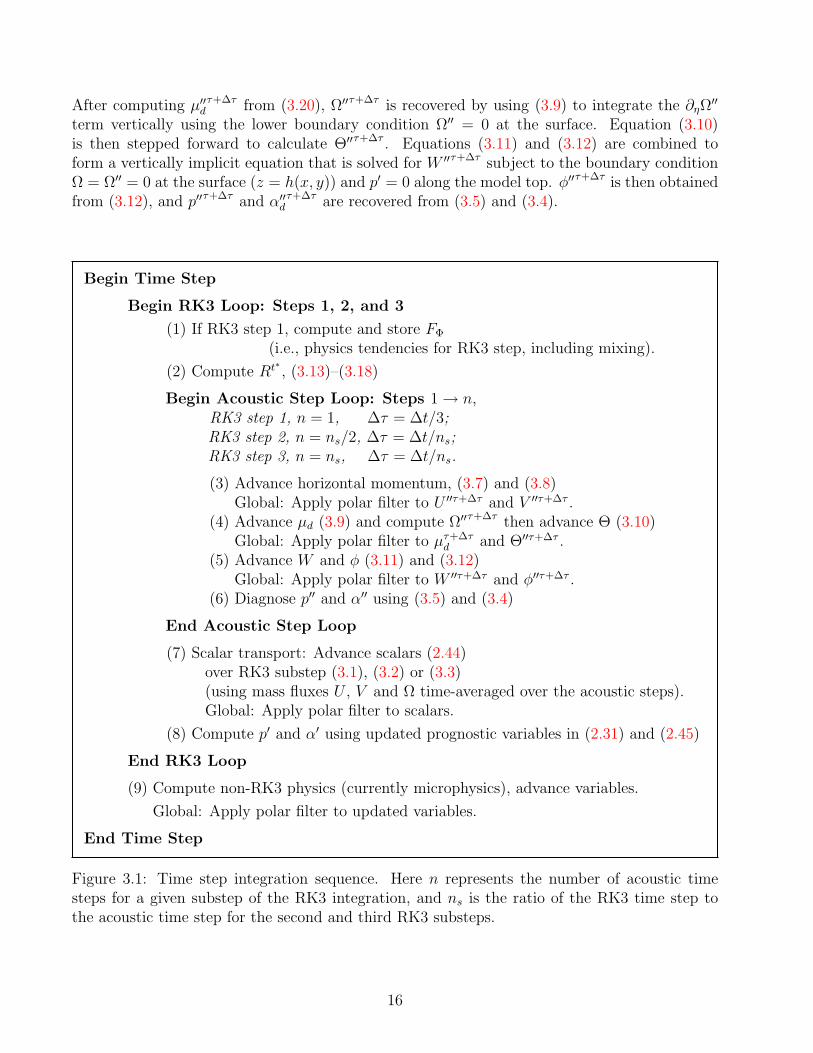
Figure 3.1: Time step integration sequence. Here n represents the number of acoustic timesteps for a given substep of the RK3 integration, and ns is the ratio of the RK3 time step tothe acoustic time step for the second and third RK3 substeps.

16

3.1.3 Full Time-Split Integration Sequence

The time-split RK3 integration technique is summarized in Figure 3.1. It consists of two primaryloops— an outer loop for the large-time-step Runge-Kutta integration, and an inner loop forthe acoustic mode integration.

In the RK3 scheme, physics can be integrated within the RK3 time integration (using a timeforward step, i.e., step (1) in Fig. 3.1, or the RK3 time integration if higher temporal accuracyis desired, i.e., in step (2)— implying a physics evaluation every RK3 substep) or external to itusing additive timesplitting, i.e., step (9).

Within the acoustic integration, the acoustic time step ∆τ is specified by the user throughthe choice of ns (see Section 3.3.2). Within the first RK3 substep, however, a single acoustictime step is used to advance the solution regardless of ns. Within the full RK3-acoustic timesplitintegration, this modified acoustic time step does not impose any additional stability constraints(see Wicker and Skamarock, 2002).

The major costs in the model arise from the evaluation of the right hand side terms Rt∗ in

(3.7) – (3.12). The efficiency of the RK3 timesplit scheme arises from the fact that the RK3time step ∆t is much larger than the acoustic time step ∆τ , hence the most costly evaluationsare only performed in the less-frequent RK3 steps.

3.1.4 Diabatic Forcing

Within the RK3 integration sequence outlined in Fig. 3.1, the RHS term Rt∗Θ in the thermo-

dynamic equation (3.10) contains contributions from the diabatic physics tendencies that arecomputed in step (1) at the beginning of the first RK3 step. This diabatic forcing is integratedwithin the acoustic steps (specifically, in step 4 in the time integration sequence shown in Fig.3.1). Additional diabatic contributions are integrated in an additive-time-split manner in step(9) after the RK3 update is complete. Thus, the diabatic forcing computed in step (9) (themicrophysics in the current release of the ARW) does not appear in R

t∗Θ from (3.10) in the

acoustic integration. We have discovered that this time splitting can excite acoustic waves andcan give rise to noise in the solutions for some applications. Note that the non-RK3 physics areintegrated in step (9) because balances produced in the physics are required at the end of thetime step (e.g., the saturation adjustment in the microphysics). So while moving these non-RK3physics into step (1) would eliminate the noise, the balances produced by these physics wouldbe altered.

We have found that the excitation of the acoustic modes can be circumvented while leavingthe non-RK3 physics in step (9) by using the following procedure that is implemented in theARW. In step (1) of the integration procedure (Fig. 3.1), an estimate of the diabatic forcingof Θ arising from the non-RK3 physics in step (9) is included in the diabatic forcing termR

t∗Θ in (3.10) (which is advanced in step 4). This estimated diabatic forcing is then removed

from the updated Θ after the RK3 integration is complete and before the evaluation of thenon-RK3 physics in step (9). We use the diabatic forcing from the previous time step as theestimated forcing; hence this procedure results in few additional computations outside of savingthe diabatic forcing between time steps.

17

3.1.5 Hydrostatic Option

A hydrostatic option is available in the ARW solver. The time-split RK3 integration techniquesummarized in Fig. 3.1 is retained, including the acoustic step loop. Steps (5) and (6) in theacoustic-step loop, where W and φ are advanced and p

and α are diagnosed, are replaced

by the following three steps. (1) Diagnose the hydrostatic pressure using the definition of thevertical coordinate

δηph =αd

αµd =

1 +

qm

µd.

(2) Diagnose αd using the equation of state (2.31) and the prognosed θ. (3) Diagnose thegeopotential using the hydrostatic equation

δηφ = −µdα

d − µ

dαd.

The vertical velocity w can be diagnosed from the geopotential equation, but it is not needed inthe solution procedure. The acoustic step loop advances gravity waves, including the externalmode, and the Lamb wave when the hydrostatic option is used.

3.2 Spatial Discretization

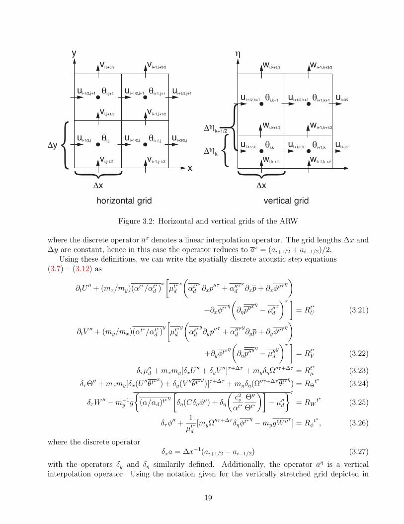
The spatial discretization in the ARW solver uses a C grid staggering for the variables as shownin Fig. 3.2. That is, normal velocities are staggered one-half grid length from the thermo-dynamic variables. The variable indices, (i, j, k) indicate variable locations with (x, y, η) =(i∆x, j∆y, k∆η). We will denote the points where θ is located as being mass points, and like-wise we will denote locations where u, v, and w are defined as u points, v points, and w points,respectively. Not shown in Fig. 3.2 are the column mass µ, defined at the (i, j) points (masspoints) on the discrete grid, the geopotential φ that is defined at the w points, and the moisturevariables qm are defined at the mass points. The diagnostic variables used in the model, thepressure p and inverse density α, are computed at mass points. The grid lengths ∆x and ∆y

are constants in the model formulation; changes in the physical grid lengths associated with thevarious projections to the sphere are accounted for using the map factors introduced in Section2.4. The vertical grid length ∆η is not a fixed constant; it is specified in the initialization. Theuser is free to specify the η values of the model levels subject to the constraint that η = 1 at thesurface, η = 0 at the model top, and η decreases monotonically between the surface and modeltop. Using these grid and variable definitions, we can define the spatial discretization for theARW solver.

3.2.1 Acoustic Step Equations

We begin by defining the column-mass-coupled variables relative to the uncoupled variables.The vertical velocity is staggered only in k, so it can be coupled directly to the column masswith no averaging or interpolation. The horizontal velocities are horizontally staggered relativeto the column mass such that the continuous variables are represented discretely as

U =µdu

my→ µd

xu

myx , V =

µdv

mx→ µd

yv

mxy ,

18

x

y

!i,j+1 !i+1,j+1

!i,j !i+1,jui-1/2,j ui+1/2,j

ui+1/2,j+1ui-1/2,j+1 ui+3/2,j+1

ui+3/2,j

vi,j-1/2 vi+1,j-1/2

vi+1,j+1/2

vi+1,j+3/2

vi,j+1/2

vi,j+3/2

horizontal grid vertical grid

"y

"x

#

ui-1/2,k+1 !i,k+1 !i+1,k+1ui+1/2,k+1 ui+3/2

!i,k !i+1,kui-1/2,k ui+1/2,k ui+3/2,

wi,k-1/2 wi+1,k-1/2

wi+1,k+3/2

wi+1,k+1/2wi,k+1/2

wi,k+3/2

"#k

"x

"#k+1/2

Figure 3.2: Horizontal and vertical grids of the ARW

where the discrete operator ax denotes a linear interpolation operator. The grid lengths ∆x and

∆y are constant, hence in this case the operator reduces to ax = (ai+1/2 + ai−1/2)/2.

Using these definitions, we can write the spatially discrete acoustic step equations(3.7) – (3.12) as

∂tU + (mx/my)(αt∗/αt∗

d )xµ

t∗d

x

αt∗d

x∂xp

τ + αdτ x

∂xp + ∂xφτ η

+∂xφt∗

η

∂ηpx

η− µ

d

xτ

= Rt∗

U (3.21)

∂tV + (my/mx)(αt∗/αt∗

d )yµ

t∗d

y

αt∗d

y∂yp

τ + αdτ y

∂yp + ∂yφτ η

+∂yφt∗

η

∂ηpy

η− µ

d

yτ

= Rt∗

V (3.22)

δτµd + mxmy[δxU

+ δyV]τ+∆τ + myδηΩ

τ+∆τ = Rt∗

µ (3.23)

δτΘ + mxmy[δx(U

θt∗

x) + δy(V

θt∗

y)]τ+∆τ + myδη(Ω

τ+∆τθt∗

η) = RΘ

t∗ (3.24)

δτW −m

−1y g

(α/αd)t∗

ηδη(Cδηφ

) + δη

c2s

αt∗Θ

Θt∗

− µ

d

τ

= RWt∗ (3.25)

δτφ +

1

µt∗d

[myΩτ+∆τ

δηφt∗

η −mygW τ ] = Rφt∗, (3.26)

where the discrete operatorδxa = ∆x

−1(ai+1/2 − ai−1/2) (3.27)

with the operators δy and δη similarily defined. Additionally, the operator aη is a vertical

interpolation operator. Using the notation given for the vertically stretched grid depicted in

19

Fig. 3.2, it is defined as

aη|k+1/2 =

1

2

∆ηk

∆ηk+1/2ak+1 +

∆ηk+1

∆ηk+1/2ak

. (3.28)

This operator vertically interpolates variables on mass levels k to the w levels (k + 12). It should

be noted that the vertical grid is defined such that vertical interpolation from w levels to masslevels reduces to a

ηk = (ak+1/2 + ak−1/2)/2 (see Fig. 3.2).

The RHS terms in the discrete acoustic step equations for momentum (3.21), (3.22) and(3.25) are discretized as

Rt∗

U = −(mx/my)(α/αd)xµd

x(∂xφη + αd

x∂xp

+ αd

x∂xp) + ∂xφ

η(∂ηp

xη− µ

d

x)

+ FUcor + advection + mixing + physics, (3.29)

Rt∗

V = −(my/mx)(α/αd)yµd

y(∂yφη + αd

y∂yp

+ αd

y∂yp) + ∂yφ

η(∂ηp

yη− µ

d

y)

+ FVcor + advection + mixing + physics, (3.30)

Rt∗

W = m−1y g(α/αd)

η[δηp

+µdqmη]−m

−1y µ

dg

+ FWcor + advection + mixing + buoyancy + physics. (3.31)

3.2.2 Coriolis and Curvature Terms

The terms FUcor , FVcor , and FWcor in (3.29) – (3.31) represent Coriolis and curvature effects inthe equations using the isotropic map projections (Lambert conformal, polar stereographic, andMercator) where mx = my = m. These terms in continuous form are given in (2.32) – (2.34).Their spatial discretization is

FUcor = +f

x+ u

xδym− v

yδxm

xV

xy − exW

xηcos αr

x − uWxη

re, (3.32)

FVcor = −f

y+ u

xδym− v

yδxm

yU

xy+ e

yW

yηsin αr

y − vWyη

re, (3.33)

FWcor = +e(Uxη

cos αr − Vyη

sin αr) +

u

xηU

xη+ v

yηV

yη

re

. (3.34)

Here the operators ()xy

= ()xy

, and likewise for ()xη

and ()yη

.For the non-isotropic latitude longitude projection, the Coriolis and curvature terms given

in (2.35) and (2.36) are discretized as

FUcor =mx

my

f

xV

xy+

uVxy

retan ψ

− e

xW

xηcos αr

x − uWxη

re, (3.35)

FVcor =my

mx

−f

yU

xy − uxy

Uxy

retan ψ + e

yW

yηsin αr

y − vWyη

re

, (3.36)

FWcor = +e(Uxη

cos αr − (mx/my)Vyη

sin αr) +

u

xηU

xη+ (mx/my)vyη

Vyη

re

. (3.37)

20

3.2.3 Advection

The advection terms in the ARW solver are in the form of a flux divergence and are a subset ofthe RHS terms in equations (3.13) – (3.18):

Rt∗

Uadv=−mx[∂x(Uu) + ∂y(V u)] + ∂η(Ωu) (3.38)

Rt∗

Vadv=−my[∂x(Uv) + ∂y(V v)] + (mx/my)∂η(Ωv) (3.39)

Rt∗

µadv=−mxmy[∂xU + ∂yV ] + my∂ηΩ (3.40)

Rt∗

Θadv=−mxmy[∂x(Uθ) + ∂y(V θ)]−my∂η(Ωθ) (3.41)

Rt∗

Wadv=− (mxmy/my)[∂x(Uw) + ∂y(V w)] + ∂η(Ωw) (3.42)

Rt∗

φadv=− µ

−1d [mxmy(U∂xφ + V ∂yφ) + myΩ∂ηφ]. (3.43)

For the mass conservation equation, the flux divergence is discretized using a 2nd-order centeredapproximation:

Rt∗

µadv= −mxmy[δxU + δyV ]t

∗+ myδηΩ

t∗. (3.44)

In the current version of the ARW, the advection of vector quantities (momentum) and scalarsis performed using the RK3 time integration as outlined in Fig. 3.1. The spatial discretizationused in this approach is outlined in the next section. For many applications it is desirable touse positive definite or monotonic advection schemes for scalar transport.

RK3 Advection

2nd through 6th order accurate spatial discretizations of the flux divergence are available in theARW for momentum, scalars and geopotential using the RK3 time-integration scheme (scalaradvection option 1, step 7 in the time-split integration sequence in Fig. 3.1). The discreteoperators can be illustrated by considering the flux divergence equation for a scalar q in itsdiscrete form:

Rt∗

qadv= −mxmy[δx(Uq

xadv) + δy(V qyadv)]−myδη(Ωq

ηadv). (3.45)

As in the pressure gradient discretization, the discrete operator is defined as

δx(Uqxadv) = ∆x

−1(Uq

xadv)i+1/2 − (Uqxadv)i−1/2

. (3.46)

The different order advection schemes correspond to different definitions for the operator qxadv .

The even order operators (2nd, 4th, and 6th) are

2nd order: (qxadv)i−1/2 =1

2(qi + qi−1)

4th order: (qxadv)i−1/2 =7

12(qi + qi−1)−

1

12(qi+1 + qi−2)

6th order: (qxadv)i−1/2 =37

60(qi + qi−1)−

2

15(qi+1 + qi−2) +

1

60(qi+2 + qi−3),

21

and the odd order operators (3rd and 5th) are

3rd order: (qxadv)i−1/2 = (qxadv)4th

i−1/2

+ sign(U)1

12

(qi+1 − qi−2)− 3(qi − qi−1)

5th order: (qxadv)i−1/2 = (qxadv)6th

i−1/2

− sign(U)1

60

(qi+2 − qi−3)− 5(qi+1 − qi−2) + 10(qi − qi−1)

.

The even-order advection operators are spatially centered and thus contain no implicit dif-fusion outside of the diffusion inherent in the RK3 time integration. The odd-order schemes areupwind-biased, and the spatial discretization is inherently diffusive. The behavior of the up-wind schemes is easily understood by expanding (3.46) using the 5th order operator, assuminga constant mass flux U and multiplying by the timestep ∆t:

∆tδx(Uqxadv) = ∆tδ(Uq)|6th −

U∆t

∆x

1

60(−qi−3 + 6qi−2 − 15qi−1 + 20qi − 15qi+1 + 6qi+2 − qi+3)

= ∆tδ(Uq)|6th − Cr

60∆x

6 ∂6q

∂x6+ higher order terms

Similarly, we can expand (3.46) using the 3rd order operator:

∆tδx(Uqxadv) = ∆tδ(Uq)|4th +

Cr

12∆x

4 ∂4q

∂x4+ higher order terms

As is evident in their formulation, the odd-order schemes are comprised of the next higher (even)order centered scheme plus an upwind term that, for a constant transport mass flux, is a diffusionterm of that next higher (even) order with a hyper-viscosity proportional to the Courant number(Cr). The diffusion term is the leading order error term in the flux divergence discretization.Further details concerning RK3 advection can be found in Wicker and Skamarock (2002)

Positive-Definite Limiter for RK3 Advection

Mixing ratios of moisture, chemical species or other tracer species should remain positive-definite, that is, negative masses should not be permitted. The Runge-Kutta transport in-tegration defined by the timestepping algorithm (3.1) – (3.3), combined with the flux divergenceoperator (3.45), is conservative but it does not guarantee positive definiteness; any negativevalues will be offset by positive mass such that mass is conserved. In many physics options,negative mixing ratios will be set to zero, and this will result in an increase in mass of thatspecies. A positive-definite flux renormalization, applied on the final Runge-Kutta transportstep (3.1), can be used to remove this unphysical effect from the RK3 scalar transport scheme.This scheme is described in Skamarock and Weisman (2008) and Skamarock (2005), and webriefly outline the ARW implementation here.

The final RK3 time integration step for transport of a scalar can be expressed as

(µφ)t+∆t = (µφ)t −∆tmxmy[δx(Uq

xadv) + δy(V qyadv)] + myδη(Ωq

ηadv)

+ ∆tµStφ (3.47)

22

where the flux divergence is evaluated using the (**) time level predicted in RK3 step (3.2).The positive-definite flux renormalization replaces (3.2) with the following two steps. First, thescalar mixing ratio is updated using the tendency derived from the model physics and source/sinkterms.

(µφ)∗∗∗ = (µφ)t + ∆tµStφ (3.48)

where we denote this new predictor as (µφ)∗∗∗. Second, the full update is computed using a fluxdivergence composed of a first-order upwind flux plus a higher order correction:

(µφ)t+∆t = (µφ)∗∗∗ −∆t

mxmy(δx

(Uq

xadv)1 + R(Uqxadv)

+δy

(V q

yadv)1 + R(V qyadv)

)

+myδη

(Ωq

ηadv)1 + R(Ωqηadv)

. (3.49)

In (3.49), ()1 denotes a first-order upwind flux and R() denotes a renormalized higher-ordercorrection flux. The higher-order correction flux is the difference between the full RK3 flux andthe first-order upwind flux, that is,

(Uqxadv) = (Uq

xadv)1 + (Uqxadv), (3.50)

with similar definitions for (V qyadv) and (Ωq

ηadv). The correction flux is then renormalized asfollows. First, the upwind fluxes are used to perform a partial update of the scalar mass.

(µφ) = (µφ)∗∗∗ −∆tmxmy[δx(Uq

xadv)1 + δy(V qyadv)1] + myδη(Ωq

ηadv)1

This update is positive definite (and monotonic) by design because it is the first-order upwindscheme. Next, a prediction of the minimum possible values of the new-time-level species massis computed at each point by using only the outward directed fluxes (fluxes that remove massfrom the control volume),

(µφ)t+∆tmin = (µφ)−∆t

mxmy[δx(U+q

xadv) + δy(V+qyadv)] + myδη(Ω+q

ηadv)

(3.51)

where U+, V+ and Ω+ indicated the use of fluxes out of a control volume only, that is, onlythose that contribute to lowering the scalar mass. As is obvious from (3.51), the scalar mass(µφ)t+∆t

min < 0 if

(µφ) < ∆tmxmy[δx(U+q


ηadv)

For each volume where negative mass is indicated by (3.51), the fluxes are renormalized suchthat the outgoing fluxes and mass in the volume are equivalent.

R (U+qxadv) = (U+q

xadv)µφ

∆tmxmy[δx(U+q


ηadv) (3.52)

with a similar renormalization applied to the (V qyadv) and (Ωq

ηadv). If no negative mass isindicated in (3.51), the correction flux is equal to the

R (U+qxadv) = (U+q

xadv) , R (V+qyadv) = (V+q

yadv) , R (Ω+qηadv) = (Ω+q

ηadv) . (3.53)

The renormalized fluxes (3.52) and (3.53), along with the first order fluxes, are then used in theupdate equation (3.49). Note that if no renormalization is needed, the scheme (3.49) reverts tothe standard RK3 update because the definition of the correction (3.50).

23

re!"

re!"

re!"

U Vµ, W

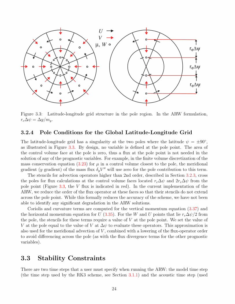
Figure 3.3: Latitude-longitude grid structure in the pole region. In the ARW formulation,re∆ψ = ∆y/my.

3.2.4 Pole Conditions for the Global Latitude-Longitude Grid

The latitude-longitude grid has a singularity at the two poles where the latitude ψ = ±90,as illustrated in Figure 3.3. By design, no variable is defined at the pole point. The area ofthe control volume face at the pole is zero, thus a flux at the pole point is not needed in thesolution of any of the prognostic variables. For example, in the finite volume discretization of themass conservation equation (3.23) for µ in a control volume closest to the pole, the meridionalgradient (y gradient) of the mass flux δyV

will use zero for the pole contribution to this term.The stencils for advection operators higher than 2nd order, described in Section 3.2.3, cross

the poles for flux calculations at the control volume faces located re∆ψ and 2re∆ψ from thepole point (Figure 3.3, the V flux is indicated in red). In the current implementation of theARW, we reduce the order of the flux operator at these faces so that their stencils do not extendacross the pole point. While this formally reduces the accuracy of the scheme, we have not beenable to identify any significant degradation in the ARW solutions.

Coriolis and curvature terms are computed for the vertical momentum equation (3.37) andthe horizontal momentum equation for U (3.35). For the W and U points that lie re∆ψ/2 fromthe pole, the stencils for these terms require a value of V at the pole point. We set the value ofV at the pole equal to the value of V at ∆ψ to evaluate these operators. This approximation isalso used for the meridional advection of V , combined with a lowering of the flux-operator orderto avoid differencing across the pole (as with the flux divergence terms for the other prognosticvariables).

3.3 Stability Constraints

There are two time steps that a user must specify when running the ARW: the model time step(the time step used by the RK3 scheme, see Section 3.1.1) and the acoustic time step (used

24

in the acoustic sub-steps of the time-split integration procedure, see Section 3.1.2). Both arelimited by Courant numbers. In the following sections we describe how to choose time steps forapplications.

3.3.1 RK3 Time Step Constraint

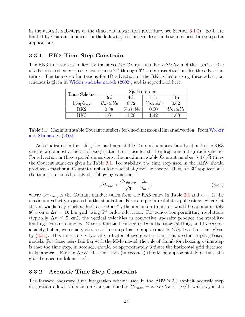
The RK3 time step is limited by the advective Courant number u∆t/∆x and the user’s choiceof advection schemes— users can choose 2nd through 6th order discretizations for the advectionterms. The time-step limitations for 1D advection in the RK3 scheme using these advectionschemes is given in Wicker and Skamarock (2002), and is reproduced here.

Spatial orderTime Scheme

3rd 4th 5th 6thLeapfrog Unstable 0.72 Unstable 0.62

RK2 0.88 Unstable 0.30 UnstableRK3 1.61 1.26 1.42 1.08

Table 3.1: Maximum stable Courant numbers for one-dimensional linear advection. From Wickerand Skamarock (2002).

As is indicated in the table, the maximum stable Courant numbers for advection in the RK3scheme are almost a factor of two greater than those for the leapfrog time-integration scheme.For advection in three spatial dimensions, the maximum stable Courant number is 1/

√3 times

the Courant numbers given in Table 3.1. For stability, the time step used in the ARW shouldproduce a maximum Courant number less than that given by theory. Thus, for 3D applications,the time step should satisfy the following equation:

∆tmax <Crtheory√

3· ∆x

umax, (3.54)

where Crtheory is the Courant number taken from the RK3 entry in Table 3.1 and umax is themaximum velocity expected in the simulation. For example in real-data applications, where jetstream winds may reach as high as 100 ms−1, the maximum time step would be approximately80 s on a ∆x = 10 km grid using 5th order advection. For convection-permitting resolutions(typically ∆x ≤ 5 km), the vertical velocities in convective updrafts produce the stability-limiting Courant numbers. Given additional constraint from the time splitting, and to providea safety buffer, we usually choose a time step that is approximately 25% less than that givenby (3.54). This time step is typically a factor of two greater than that used in leapfrog-basedmodels. For those users familiar with the MM5 model, the rule of thumb for choosing a time stepis that the time step, in seconds, should be approximately 3 times the horizontal grid distance,in kilometers. For the ARW, the time step (in seconds) should be approximately 6 times thegrid distance (in kilometers).

3.3.2 Acoustic Time Step Constraint

The forward-backward time integration scheme used in the ARW’s 2D explicit acoustic stepintegration allows a maximum Courant number Crmax = cs∆τ/∆x < 1/

√2, where cs is the

25

speed of sound. We typically use a more conservative estimate for this by replacing the limitingvalue 1/

√2 with 1/2. Thus, the acoustic time step used in the model is

∆τ < 2 · ∆x

cs. (3.55)

For example, on a ∆x = 10 km grid, using a sound speed cs = 300 ms−1, the acoustic timestep given in (3.55) is approximately 17 s. In the ARW, the ratio of the RK3 time step to theacoustic time step must be an even integer. For our example using a ∆x = 10 km grid in areal-data simulation, we would specify the RK3 time step ∆t = 60s (i.e., 25% less than the 80 sstep given by (3.54), and an acoustic time step ∆τ = 15 s (i.e., 1/4 of the RK3 step, roundingdown the ∆τ = 17 s step given by (3.55)). Note that it is the ratio of the RK3 time step to theacoustic time step that is the required input in the ARW.

3.3.3 Adaptive Time Step

The ARW model is typically integrated with a fixed timestep, that is chosen to produce astable integration. During any time in the integration, the maximum stable timestep is likelyto be larger than the fixed timestep. In ARWV3, an adaptive timestepping capability has beenintroduced that chooses the RK3 timestep based on the temporally-evolving wind fields. Theadaptively-chosen timestep is usually larger than the typical fixed timestep, hence the dynamicsintegrates faster and physics are called less often, and the time-to-completion of the simulationcan be substantially reduced.

In the adaptive timestep scheme, a target maximum Courant number Crtarget is chosen,where typically 1.1 ≤ Crtarget ≤ 1.2. The maximum Courant number in the domain at a giventime (Crdomain), computed for all the velocity components (u, v, w), is then used to computea new timestep. When the maximum Courant number in the domain is less than the targetmaximum Courant number (Crdomain < Crtarget), then the timestep can be increased and thenew timestep is computed using

∆tcurrent = min

1 + fi,

Crtarget

Crdomain

· ∆tprevious, (3.56)

where a typical value for the regulated increase is fi ≤ 5%. When the computed maxi-mum domain-wide Courant number exceeds the targeted maximum allowable Courant number(Crdomain > Crtarget), then the time step is decreased to insure model stability:

∆tcurrent = max

1− fd,

Crtarget − 0.5(Crdomain − Crtarget)

Crdomain

· ∆tprevious, (3.57)

where typically the factor to decrease the time step fd = 25%. Both a lower bound and an upperbound on the time step are enforced based on the initial settings of the time step suggested insection 3.3.1:

∆tinit = 6 · ∆x, (3.58)

∆tmin = 0.5 · ∆tinit, (3.59)

26

∆tmax = 3.0 · ∆tinit, (3.60)

∆t = min(max(∆t, ∆tmin), ∆tmax), (3.61)

to guard the time step from becoming too small or too large. The computation of the numberof acoustic time steps na, described in section 3.3.2, is handled during the first of each of theRK3 model integration steps:

na = max

2 · 300 · ∆t

∆x+ 1, 4

. (3.62)

For a simulation using nests, the fine-grid domain must maintain an integer number oftime steps within a single model integration step from the parent. At each of the starting modelintegration steps for the child grid, those integration steps when the time on the fine-grid domainequals the time on the parent’s domain, the adaptive time step algorithm is conducted for thefine grid. Note that the ratio of the nominal grid distance between the parent and the childdoes not necesarily imply that same ratio between the model integration time steps.

3.3.4 Map Projection Considerations

For ARW configurations using the Lambert conformal, polar stereographic, or Mercator projec-tions, the timestep constraints is determined by the smallest physical horizontal grid spacing,i.e. min(∆x/mx, ∆y/my). For global applications, the grid distance used to determine thetimestep should be ∆x/mx evaluated at the computational latitude at which the polar filtersare activated. Polar filtering is discussed in section 4.1.

27

Chapter 4

Turbulent Mixing and Model Filters

A number of formulations for turbulent mixing and filtering are available in the ARW solver.Some of these filters are used for numerical reasons. For example, divergence damping is usedto filter acoustic modes from the solution and polar filtering is used to reduce the timesteprestriction arising from the converging gridlines of the latitude-longitude grid. Other filters aremeant to represent sub-grid turbulence processes that cannot be resolved on the chosen grid.These filters remove energy from the solution and are formulated in part on turbulence theoryand observations, or represent energy sink terms in some approximation to the Euler equation.In this section, we begin by outlining the formulation and discretization of turbulent mixingprocesses in the ARW solver commonly associated with sub-gridscale turbulence as parame-terized in cloud-scale models— the second-order horizontal and vertical mixing. In large-scalemodels and most NWP models, vertical mixing is parameterized within the planetary boundarylayer (PBL) physics. Vertical mixing parameterized within the PBL physics is described later inChapter 8. Here we note that, when a PBL parameterization is used, all other vertical mixingis disabled. Following the outline of turbulent mixing parameterizations in this chapter, othernumerical filters available in the ARW solver are described.

4.1 Latitude-Longitude Global Grid and Polar Filtering

Polar filtering is used to reduce the timestep restriction associated with the gridlines that con-verge as they approach the poles of the latitude-longitude grid; the converging gridlines reducethe longitudinal gridlength, and thus the stable timestep for transport, discussed in Section3.3.1, and for acoustic waves, discussed in Section 3.3.2, will be reduced.

Polar filtering a given variable is accomplished by first applying a 1D Fourier transform tothe variable on a constant computational-grid latitude circle (the forward transform), wherethe field is periodic. The Fourier coefficients with wavenumbers above a prescribed thresholdare truncated, after which a transformation back to physical space is applied (the backwardtransform), completing the filter step.

A filter application can be written as

φ(k)filtered = a(k) φ(k), for all k,

where φ(k) and φ(k)filtered are the Fourier coefficients for the generic variable φ before and afterfiltering, and a(k) are the filter coefficients defined as a function of the dimensionless wavenumber

29

k. The ARW polar filter coefficients a(k) for the Fourier amplitudes are

a(k) = min

1., max

0.,

cos ψ

cos ψo

2 1

sin2(πk/n)

where ψ is the latitude on the computational grid, ψo is the latitude above which the polar filteris applied (the filter is applied for |ψ| > ψo), and n is the number of grid points in the latitudecircle. For even n, the grid admits wavenumber k = 0 and dimensionless wavenumbers ±k fork = 1 → n/2 − 1, and the 2∆ wave k = n/2. For odd n, the grid admits wavenumber k = 0,and dimensionless wavenumbers ±k for k = 1 → (n− 1)/2.

Polar filter applications within the split-explicit RK3 time integration scheme are given inFigure 3.1. Within the acoustic steps, the filter is applied to U

τ+∆τ and Vτ+∆τ immediately

after the horizontal momentum is advanced, to µτ+∆τd and Θτ+∆τ immediately after the column

mass and the potential temperature are advanced, and to Wτ+∆τ and φ

τ+∆τ after the verticallyimplicit part of the acoustic step is complete. The polar filter is also applied to the scalars afterthey are advanced every RK3 sub-step (3.1)-(3.3) and after the microphysics step.

The prognostic variables are coupled with the column mass µ when filtered, and in this waymass is conserved. An exception to this is the geopotential φ which is filtered without beingcoupled. The Fourier filtering is conservative, but it is not monotonic or positive definite. Asnoted in the ARW stability discussion in Section 3.3.4, timestep stability should be based on thelongitudinal gridlength where the polar filters are activated, (∆x/mx)|ψo . The positive definitetransport option, presented in Section 3.2.3, will not necessarily produce positive-definite resultsbecause of the converging gridlines and should not be used.

4.2 Explicit Spatial Diffusion

The ARW solver has three formulations for spatial dissipation— diffusion along coordinatesurfaces, diffusion in physical (x, y, z) space, and a sixth-order diffusion applied on horizontalcoordinate surfaces. In the following sections we present the diffusion operators for the the firsttwo formulations, followed by the four separate formulations that can be used to compute theeddy viscosities and a description of the prognostic turbulent kinetic energy (TKE) equationused in one set of these formulations. The sixth order spatial filter is described at the end ofthis section. In these formulations, the horizontal (Kh) and vertical (Kv) eddy viscosities aredefined at scalar points on the staggered model grid.

4.2.1 Horizontal and Vertical Diffusion on Coordinate Surfaces

For any model variable, horizontal and vertical second order spatial filtering on model coordinatesurfaces is considered part of the RHS terms in the continuous equations (2.38) – (2.44) and canbe expressed as follows for a model variable a:

∂t(µda) = ... + µd

mx∂x(mxKh∂xa) + my∂y(myKh∂ya)

+ g

2(µdα)−1∂η(Kvα

−1∂ηa). (4.1)

30

For the horizontal and vertical momentum equations, (4.1) is spatially discretized as

∂tU = ... + µdxmx

xδx(mxKhδxu) + δy(my

xyKh

xyδyu)

+ m

−1y g

2(µdxα

x)−1δη(Kv

xη(αxη)−1

δηu)

∂tV = ... + µdymy

yδx(mx

xyKh

xyδxv) + δy(myKhδyv)

+ m

−1x g

2(µdyα

y)−1δη(Kv

yη(αyη)−1

δηv)

∂tW = ... + µdmx

δx(mx

xKh

xηδxw) + δy(my

yKh

yηδyw)

+ m

−1y g

2(µdαη)−1

δη(Kvα−1

δηw).

The spatial discretization for a scalar q, defined at the mass points, is

∂t(µdq) = ... +µdmxmy

δx(mx

xP−1r Kh

xδxq)+δy(my

yP−1r Kh

yδyq)

+g

2(µdα)−1δη(Kv

η(αη)−1

δηq).

In the current ARW formulation for mixing on coordinate surfaces, the horizontal eddy viscosityKh is allowed to vary in space, whereas the vertical eddy viscosity does not vary in space; hencethere is no need for any spatial averaging of Kv. Additionally, note that the horizontal eddyviscosity Kh is multiplied by the inverse turbulent Prandtl number P

−1r for horizontal scalar

mixing.

4.2.2 Horizontal and Vertical Diffusion in Physical Space

Coordinate Metrics

We use the geometric height coordinate in this physical space formulation. The coordinatemetrics are computed using the prognostic geopotential in the ARW solver. At the beginningof each Runge-Kutta time step, the coordinate metrics are evaluated as part of the overallalgorithm. The definitions of the metrics are

zx = g−1

δxφ and zy = g−1

δyφ.

These metric terms are defined on w levels, and (zx, zy) are horizontally coincident with (u,v)points. Additionally, the vertical diffusion terms are evaluated directly in terms of the geometricheight, avoiding the need for metric terms in the vertical.

Continuous Equations

The continuous equations for evaluating diffusion in physical space, using the velocity stresstensor, are as follows for horizontal and vertical momentum:

∂tU = ... −mx

∂xτ11 + ∂yτ12 − ∂z(zxτ11 + zyτ12)

− ∂zτ13 (4.2)

∂tV = ... −my

∂xτ12 + ∂yτ22 − ∂z(zxτ12 + zyτ22)

− ∂zτ23 (4.3)

∂tW = ... −my

∂xτ13 + ∂yτ23 − ∂z(zxτ13 + zyτ23)

− ∂zτ33. (4.4)

The stress tensor τ can be written as follows:

τ11 = −µdKhD11

τ22 = −µdKhD22

τ33 = −µdKvD33

τ12 = −µdKhD12

τ13 = −µdKvD13

τ23 = −µdKvD23.

31

Symmetry sets the remaining tensor values; τ21 = τ12, τ31 = τ13, and τ32 = τ23. The stress tensorτ is calculated from the deformation tensor D. The continuous deformation tensor is defined as

D11 = 2 mxmy

∂x(m

−1y u)− zx∂z(m

−1y u)

D22 = 2 mxmy

∂y(m

−1x v)− zy∂z(m

−1x v)

D33 = 2 ∂zw

D12 = mxmy

∂y(m

−1y u)− zy∂z(m

−1y u) + ∂x(m

−1x v)− zx∂z(m

−1x v)

D13 = mxmy

∂x(m

−1y w)− zx∂z(m

−1y w)

+∂z(u)

D23 = mxmy

∂y(m

−1y w)− zy∂z(m

−1y w)

+∂z(v).

The deformation tensor is symmetric, hence D21 = D12, D31 = D13, and D32 = D23.The diffusion formulation for scalars is

∂t(µdq) = ... +mx

∂x − ∂zzx

µdmxKh(∂x − zx∂z)

+

my

∂y − ∂zzy

µdmyKh(∂y − zy∂z)

+ ∂zµdKv∂z

q. (4.5)

Spatial Discretization

Using the definition of the stress tensor, the spatial discretization of the ARW physical-spacediffusion operators for the horizontal and vertical momentum equations (4.2) - (4.4) are

∂tU = ... −mxxδxτ11 + δyτ12 − δz(zxτ11

xη + zyxy

τ12yη)

− δzτ13

∂tV = ... −myyδyτ22 + δxτ12 − δz(zyτ22

yη + zxxy

τ12xη)

− δzτ23

∂tW = ... −mx

δxτ13 + δyτ23 − δz(zx

xητ13

xη + zyyη

τ23yη)

− δzτ33.

The discrete forms of the stress tensor and deformation tensor are

τ11 = −µdKhD11

τ22 = −µdKhD22

τ33 = −µdKvD33

τ12 = −µdxy

Khxy

D12

τ13 = −µdxKv

xηD13

τ23 = −µdyKv

yηD23,

and

D11 = 2 mxmy

δx(m−1

y

xu)− zx

xηδz(m−1

y

xu)

D22 = 2 mxmy

δy(m−1

x

yv)− zy

xηδz(m−1

x

yv)

D33 = 2 δzw

D12 = (mxmyxy)

δy(m−1

y

xu)− zy

xηδz(m−1

y

xu)

yη+ δx(m−1

x

yv)− zx

yηδz(m−1

x

yv)

xη

D13 = mxmy

δx(m

−1y w)− zxδz(m−1w)

xη+δzu

D23 = mxmy

δy(m

−1y w)− zyδz(m−1

y w)yη

+δzv.

32

The spatial discretization for the scalar diffusion (4.5) is

∂t(µdq) = ... + mx

δx

µd

xH1(q)

− µdδz

zx

xH1(q)

xη

+ my

δy

µd

yH2(q)

− µdδz

zy

yH2(q)

yη

+ µdδz

Kv

ηδzq

,

where

H1(q) = mxxKh

xδxq − zxδz(q

xη),

H2(q) = myyKh

yδyq − zyδz(q

yη).

4.2.3 Computation of the Eddy Viscosities

There are four options for determining the eddy viscosities Kh and Kv in the ARW solver.

External specification of Kh and Kv

Constant values for Kh and Kv can be input in the ARW namelist.

Kh determined from the horizontal deformation

The horizontal eddy viscosity Kh can be determined from the horizontal deformation using aSmagorinsky first-order closure approach. In this formulation, the eddy viscosity is defined anddiscretized as

Kh = C2s l

2

0.25(D11 −D22)

2 + D212

xy 1

2

.

The deformation tensor components have been defined in the previous section. The length scalel = (∆x∆y)1/2 and Cs is a constant with a typical value Cs = 0.25. For scalar mixing, theeddy viscosity is divided by the turbulent Prandtl number Pr that typically has a value of 1/3(Deardorff, 1972). This option is most often used with a planetary boundary layer scheme thatindependently handles the vertical mixing.

3D Smagorinsky Closure

The horizontal and vertical eddy viscosities can be determined using a 3D Smagorinsky turbu-lence closure. This closure specifies the eddy viscosities as

Kh,v = C2s l

2h,v max

0.,

D

2 − P−1r N

21/2

, (4.6)

where

D2 =

1

2

D

211 + D

222 + D

233

+

D12

xy2+

D13

xη2+

D23

yη2,

and N is the Brunt-Vaisala frequency; the computation of N , including moisture effects, isoutlined in Section 4.2.4.

33

Two options are available for calculating the mixing length lh,v in (4.6). An isotropic lengthscale (appropriate for ∆x, ∆y ∆z) can be chosen where lh,v = (∆x∆y∆z)1/3 and thus Kh =Kv = K. The anisotropic option (appropriate for ∆x, ∆y >> ∆z) sets the horizontal mixinglength lh =

√∆x∆y in the calculation of the horizontal eddy viscosity Kh using (4.6), and

lv = ∆z for the calculation of the vertical eddy viscosity Kv using (4.6).Additionally, the eddy viscosities for scalar mixing are divided by the turbulent Prandtl

number Pr = 1/3.

Prognostic TKE Closure

For the predicted turbulent kinetic energy option (TKE; see section 4.2.4), the eddy viscositiesare computed using

Kh,v = Cklh,v

√e,

where e is the turbulent kinetic energy (a prognostic variable in this scheme), Ck is a constant(typically 0.15 < Ck < 0.25), and l is a length scale.

If the isotropic mixing option is chosen,

lh,v = min(∆x∆y∆z)1/3

, 0.76√

e/N

for N2

> 0,

lh,v = (∆x∆y∆z)1/3 for N2 ≤ 0

(see section 4.2.4 for the calculation of N2). Both the horizontal and vertical eddy viscosities

are multiplied by an inverse turbulent Prandtl number P−1r = 1 + 2l/(∆x∆y∆z)1/3 for scalar

mixing. In this case (lcr > ∆x) the horizontal and vertical eddy viscosities are equivalent.If the anisotropic mixing option is chosen, then lh =

√∆x∆y for the calculation of Kh. For

calculating Kv,

lv = min∆z, 0.76

√e/N

for N

2> 0,

lv = ∆z for N2 ≤ 0.

The eddy viscosity used for mixing scalars is divided by a turbulent Prandtl number Pr. ThePrandtl number is 1/3 for the horizontal eddy viscosity Kh, and P

−1r = 1+2l/∆z for the vertical

eddy viscosity Kv.

4.2.4 TKE equation for the 1.5 Order Turbulence Closure

The prognostic equation governing the evolution of the turbulent kinetic energy e is

∂t(µde) + (∇ · Ve)η = µd( shear production + buoyancy + dissipation ). (4.7)

The time integration and the transport terms in (4.7) are integrated in the same manner as forother scalars (as described in Chapter 3). The right-hand side source and sink terms for e aregiven as follows.

Shear Production

The shear production term in (4.7) can be written as

shear production = KhD211 + KhD

222 + KvD

233 + KhD

212

xy+ KvD

213

xη+ KvD

223

yη.

34

Buoyancy

The buoyancy term in the TKE equation (4.7) is written as

buoyancy = −KvN2,

where the Brunt-Vaisala frequency N is computed using either the formula for a moist saturatedor unsaturated environment:

N2 = g

A∂zθe − ∂zqw

if qv ≥ qvs or qc ≥ 0.01 g/Kg;

N2 = g

1

θ∂zθ + 1.61∂zqv − ∂zqw

if qv < qvs or qc < 0.01 g/Kg.

The coefficient A is defined as

A = θ−1

1 + 1.61Lqv

RdT

1 + L2qv

CpRvT 2

,

where qw represents the total water (vapor + all liquid species + all ice species), L is the latentheat of condensation and is the ratio of the molecular weight of water vapor to the molecularweight of dry air. θe is the equivalent potential temperature and is defined as

θe = θ

1 +

Lqvs

CpT

,

where qvs is the saturation vapor mixing ratio.

Dissipation

The dissipation term in (4.7) is

dissipation = −Ce3/2

l,

where

C = 1.9 Ck +(0.93− 1.9 Ck) l

∆s,

∆s = (∆x∆y∆z)1/3, and

l = min(∆x∆y∆z)1/3

, 0.76√

e/N.

4.2.5 Sixth-Order Spatial Filter on Coordinate Surfaces

A sixth order spatial filter is available that is applied on horizontal coordinate surfaces. Thediffusion scheme is that proposed by Xue (2000). Its application in the ARW is described byKnievel et al. (2007). The filter can be expressed as

∂t(µda) = ...β 2−6

2∆t

∆x

6δx(µd

xFx) + ∆y

6δy(µd

yFy)

(4.8)

35

The diffusive fluxes Fx = δ5x(a) and Fy = δ

5y(a). β is a user-specified filtering coefficient repre-

senting the damping applied to 2∆ waves for each filter application.The user can choose to enforce monotonicity in the filtering. In the monotonic option, the

diffusive fluxes are set to zero if up-gradient diffusion is indicated – Fx = 0 if Fx δx(a) < 0 andFy = 0 if Fy δy(a) < 0. Note that the filter is applied in computational space; map factors arenot taken into account and the filter parameter β is dimensionless. Thus, the filter scales withthe timestep and gridsize and it does not conserve scalar mass. This explicit diffusion acts onall three components of wind, potential temperature, all moisture variables and passive scalars,and subgrid turbulence kinetic energy. Further details can be found in Knievel et al. (2007).

4.3 Filters for the Time-split RK3 scheme

Three filters are used in the ARW time-split RK3 scheme apart from those in the model physics:three-dimensional divergence damping (an acoustic model filter); an external-mode filter thatdamps vertically-integrated horizontal divergence; and off-centering of the vertically implicitintegration of the vertical momentum equation and geopotential equation. Each of these isdescribed in the following sections.

4.3.1 Three-Dimensional Divergence Damping

The damping of the full mass divergence is a filter for acoustic modes in the ARW solver. This3D mass divergence damping is described in Skamarock and Klemp (1992). The filtering isaccomplished by forward weighting the pressure update in the acoustic step loop described inSection 3.1.3, step (6). The linearized equation of state (3.5) is used to diagnose the pressure atthe new time τ after the U

, V, µ

d, and Θ have been advanced. Divergence damping consists

of using a modified pressure in the computation of the pressure gradient terms in the horizontalmomentum equations in the acoustic steps (Equations (3.7) and (3.8)). Denoting the updatedvalue as p

τ , the modified pressure p∗τ used in (3.7) and (3.8) can be written as

p∗τ = p

τ + γd

p

τ − pτ−∆τ

, (4.9)

where γd is the damping coefficient. This modification is equivalent to inserting a horizontaldiffusion term into the equation for the 3D mass divergence, hence the name divergence damping.A divergence damping coefficient γd = 0.1 is typically used in the ARW applications, independentof time step or grid size.

4.3.2 External Mode Filter

The external modes in the solution are damped by filtering the vertically-integrated horizontaldivergence. This damping is accomplished by adding a term to the horizontal momentumequations. The additional term added to (3.7) and (3.8) are

δτU = ... − γeδx(δτ−∆τµ

d) (4.10)

andδτV

= ... − γeδy(δτ−∆τµd). (4.11)

36

The quantity δτ−∆τµ is the vertically-integrated mass divergence (i.e., (3.20)) from the previousacoustic step (that is computed using the time τ values of U and V ), and γe is the external modedamping coefficient. An external mode damping coefficient γe = β

∆x2

∆t , β = 0.01, is typicallyused in the ARW applications, independent of time step or grid size.

4.3.3 Semi-Implicit Acoustic Step Off-centering

Forward-in-time weighting of the vertically-implicit acoustic-time-step terms damps instabilitiesassociated vertically-propagating sound waves. The forward weighting also damps instabilitiesassociated with sloping model levels and horizontally propagating sound waves (see Durran andKlemp, 1983; Dudhia, 1995). The off-centering is accomplished by using a positive (non-zero)coefficient β (3.19) in the acoustic time-step vertical momentum equation (3.11) and geopotentialequation (3.12). An off-centering coefficient β = 0.1 is typically used in the ARW applications,independent of time step or grid size.

4.4 Formulations for Gravity Wave Absorbing Layers

There are three formulations for absorbing vertically-propagating gravity waves so as to preventunphysical wave reflection off the domain upper boundary from contaminating ARW solutions.

4.4.1 Absorbing Layer Using Spatial Filtering

This formulation of the absorbing layer increases the second-order horizontal and vertical eddyviscosities in the absorbing layer using the following formulation:

Kdh =∆x

2

∆tγg cos

π

2

ztop − z

zd

,

and

Kdv =∆z

2

∆tγg cos

π

2

ztop − z

zd

.

Here γg is a user-specified damping coefficient, ztop is the height of the model top for a particulargrid column, zd is the depth of the damping layer (from the model top), and Kdh and Kdv arethe horizontal and vertical eddy viscosities for the wave absorbing layer. If other spatial filtersare being used, then the eddy viscosities that are used for the second-order horizontal andvertical eddy viscosities are the maximum of (Kh, Kdh) and (Kv, Kdv). The effect of this filteron gravity waves is discussed in Klemp and Lilly (1978), where guidance on the choice of thedamping coefficient γg can also be found.

4.4.2 Implicit Rayleigh Damping for the Vertical Velocity

Implicitly damping the vertical velocity within the implicit solution algorithm for the verticallypropagating acoustic modes has been found to be a very effective and robust absorbing layerformulation by Klemp et al. (2008). We recommend its use in both large-scale and small-scaleapplications, and in idealized and real-data applications. It has proven more effective than the

37

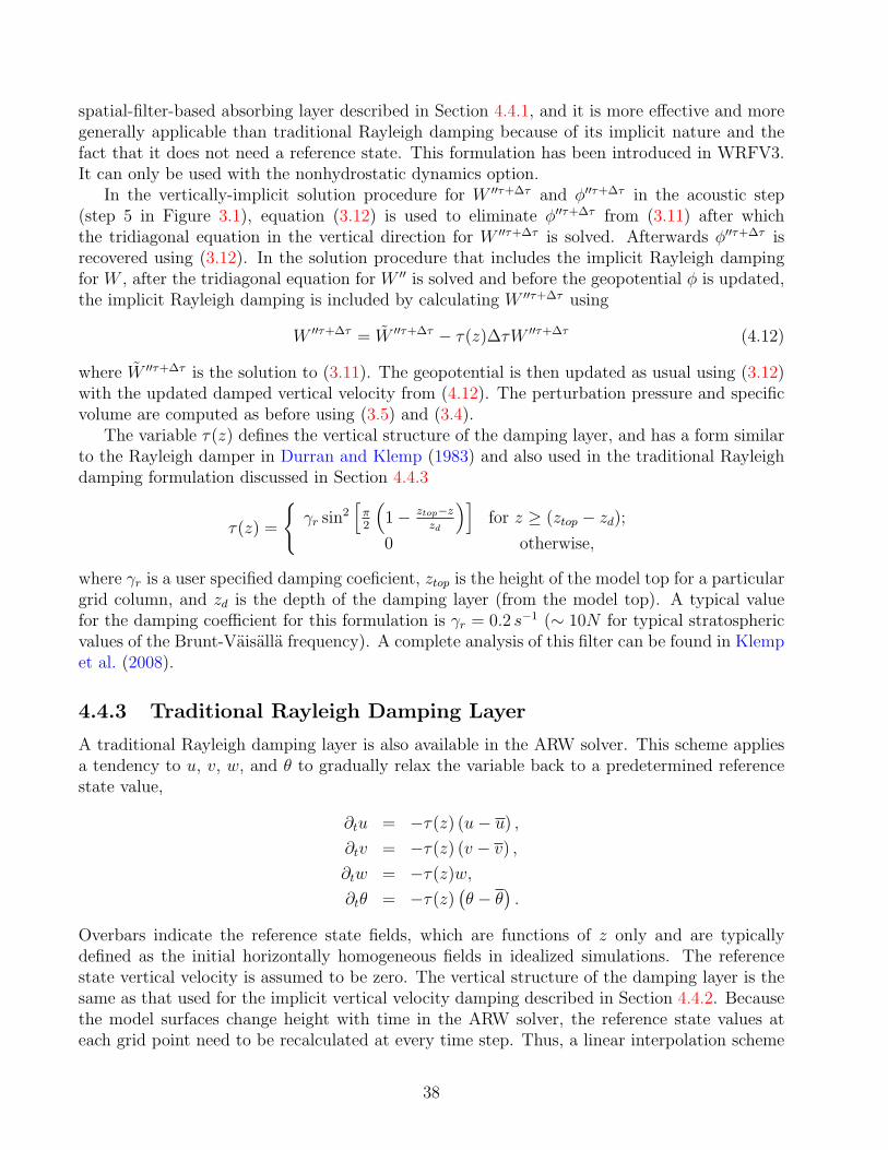
spatial-filter-based absorbing layer described in Section 4.4.1, and it is more effective and moregenerally applicable than traditional Rayleigh damping because of its implicit nature and thefact that it does not need a reference state. This formulation has been introduced in WRFV3.It can only be used with the nonhydrostatic dynamics option.

In the vertically-implicit solution procedure for Wτ+∆τ and φ

τ+∆τ in the acoustic step(step 5 in Figure 3.1), equation (3.12) is used to eliminate φ

τ+∆τ from (3.11) after whichthe tridiagonal equation in the vertical direction for W

τ+∆τ is solved. Afterwards φτ+∆τ is

recovered using (3.12). In the solution procedure that includes the implicit Rayleigh dampingfor W , after the tridiagonal equation for W

is solved and before the geopotential φ is updated,the implicit Rayleigh damping is included by calculating W

τ+∆τ using

Wτ+∆τ = W

τ+∆τ − τ(z)∆τWτ+∆τ (4.12)

where Wτ+∆τ is the solution to (3.11). The geopotential is then updated as usual using (3.12)

with the updated damped vertical velocity from (4.12). The perturbation pressure and specificvolume are computed as before using (3.5) and (3.4).

The variable τ(z) defines the vertical structure of the damping layer, and has a form similarto the Rayleigh damper in Durran and Klemp (1983) and also used in the traditional Rayleighdamping formulation discussed in Section 4.4.3

τ(z) =

γr sin2

π2

1− ztop−z

zd

for z ≥ (ztop − zd);

0 otherwise,

where γr is a user specified damping coeficient, ztop is the height of the model top for a particulargrid column, and zd is the depth of the damping layer (from the model top). A typical valuefor the damping coefficient for this formulation is γr = 0.2 s

−1 (∼ 10N for typical stratosphericvalues of the Brunt-Vaisalla frequency). A complete analysis of this filter can be found in Klempet al. (2008).

4.4.3 Traditional Rayleigh Damping Layer

A traditional Rayleigh damping layer is also available in the ARW solver. This scheme appliesa tendency to u, v, w, and θ to gradually relax the variable back to a predetermined referencestate value,

∂tu = −τ(z) (u− u) ,

∂tv = −τ(z) (v − v) ,

∂tw = −τ(z)w,

∂tθ = −τ(z)θ − θ

.

Overbars indicate the reference state fields, which are functions of z only and are typicallydefined as the initial horizontally homogeneous fields in idealized simulations. The referencestate vertical velocity is assumed to be zero. The vertical structure of the damping layer is thesame as that used for the implicit vertical velocity damping described in Section 4.4.2. Becausethe model surfaces change height with time in the ARW solver, the reference state values ateach grid point need to be recalculated at every time step. Thus, a linear interpolation scheme

38

is used to calculate updated reference state values based on the height of the model levels ateach time step.

The effect of this filter on gravity waves is discussed in Klemp and Lilly (1978), whereguidance on the choice of the damping coefficeint γr can also be found.

4.5 Other Damping

4.5.1 Vertical-Velocity Damping

This is also called w-damping. In semi-operational or operational NWP applications, the modelrobustness can be improved by detecting locations where the vertical motion approaches thelimiting Courant number for stability, and applying a Rayleigh damping term in the verticalmomentum equation to stabilize the motion. This term is non-physical and should only be usedin the situation where many, or long, model runs are being done, and there is no option for are-run with a shorter time-step if a failure occurs due to an excessively strong updraft. Thismight be the case, for example, in an operational setting where real-time forecasts have to beproduced on time to be useful. However, if this term activates frequently, consideration shouldbe given to reducing the model time-step.

The term is calculated from

Cr =

Ωdt

µdη

.

If Cr > Crβ, then∂tW = ...− µd sign(W )γw(Cr − Crβ),

where γw is the damping coefficient (typically 0.3 ms−2), and Crβ is the activation Courantnumber (typically 1.0). The ARW outputs the location of this damping when it is active.

39

Chapter 5

Initial Conditions

The ARW may be run with user-defined initial conditions for idealized simulations, or it may berun using interpolated data from either an external analysis or forecast for real-data cases. Both2D and 3D tests cases for idealized simulations are provided. Several sample cases for real-datasimulations are provided, which rely on pre-processing from an external package (usually theWRF Preprocessor System, referred to as WPS) that converts the large-scale GriB data into aformat suitable for ingest by the ARW’s real-data processor.

The programs that generate the specific initial conditions for the selected idealized or real-data case function similarly. They provide the ARW with:

• input data that is on the correct horizontal and vertical staggering;• hydrostatically balanced reference state and perturbation fields; and• metadata specifying such information as the date, grid physical characteristics, and pro-

jection details.

For neither the idealized nor the real-data cases are the initial conditions enhanced with obser-vations. However, output from the ARW system initial condition programs is suitable as inputto the WRF variational assimilation package (see Chapter 9).

5.1 Initialization for Idealized Conditions

The ARW comes with a number of test cases using idealized environments, including largeeddy simulations (em les), sea breezes (em seabreeze2d x), mountain waves (em hill2d x), squalllines (em squall2d x, em squall2d y), supercell thunderstorms (em quarter ss), gravity currents(em grav2d x), baroclinic waves (em b wave), and global domains (em heldsuarez). A briefdescription of these test cases can be found in the README test cases file provided in theARW release. The test cases include examples of atmospheric flows at fine scales (e.g., the LESexample has a grid-spacing of 100 meters and a time step of 1 second) and examples of flow atlarge scales (e.g., the Held Suarez global test case uses a grid-spacing around 600 km and a timestep of 1800 s), in addition to the traditional mesoscale and cloudscale model simulations. Thetest suite allows an ARW user to easily reproduce these known solutions. The test suite is alsothe starting point for constructing idealized flow simulations by modifying initializations thatclosely resemble a desired initialization.

Most of these tests use as input a 1D sounding specified as a function of geometric heightz (except for the baroclinic wave case that uses a 2D profile specified in [y, z]), and, with the

41

exception of the baroclinic wave test case, the sounding files are in text format that can bedirectly edited by the user. The 1D specification of the sounding in these test files requires thesurface values of pressure, potential temperature, and water vapor mixing ratio, followed by thepotential temperature, vapor mixing ratio, and horizontal wind components at some heightsabove the surface. The initialization programs for each case assume that this moist soundingrepresents an atmosphere in hydrostatic balance.

Two sets of thermodynamic fields are needed for the model— the reference state and theperturbation state (see Chapter 2 for discussion of the equations). The reference state used inthe idealized initializations is computed using the input sounding from which the moisture isdiscarded (because the reference state is dry). The perturbation state is computed using thefull moist input sounding. The procedure for computing the hydrostatically-balanced ARWreference and perturbation state variables from the input sounding is as follows. First, densityand both a dry and full hydrostatic pressure are computed from the input sounding at the inputsounding levels z. This is accomplished by integrating the hydrostatic equation vertically up thecolumn using the surface pressure and potential temperature as the lower boundary condition.The hydrostatic equation is

δzp = −ρzg(1 + (Rd/Rv)qv

z), (5.1)

where ρz is a two point average between input sounding levels, and δzp is the difference of

the pressure between input sounding levels divided by the height difference. Additionally, theequation of state is needed to close the system:

αd =1

ρd=

Rdθ

po

1 +

Rd

Rvqv

p

po

− cvcp

, (5.2)

where qv and θ are given in the input sounding. (5.1) and (5.2) are a coupled set of nonlinearequations for p and ρ in the vertical integration, and they are solved by iteration. The drypressure on input sounding levels is computed by integrating the hydrostatic relation down fromthe top, excluding the vapor component.

Having computed the full pressure (dry plus vapor) and dry air pressure on the input sound-ing levels, the pressure at the model top (pdht) is computed by linear interpolation in height(or possibly extrapolation) given the height of the model top (an input variable). The columnmass µd is computed by interpolating the dry air pressure to the surface and subtracting from itpdht. Given the column mass, the dry-air pressure at each η level is known from the coordinatedefinition (2.1), repeated here

η = (pdh − pdht)/µd where µd = pdhs − pdht,

and the pressures pdhs and pdht refer to the dry atmosphere. The potential temperature fromthe input sounding is interpolated to each of the model pressure levels, and the equation of state(5.2) is used to compute the inverse density αd. Finally, the ARW’s hydrostatic relation (2.9),in discrete form

δηφ = −αdµd

is used to compute the geopotential. This procedure is used to compute the reference state(assuming a dry atmosphere) and the full state (using the full moist sounding). The perturbationvariables are computed as the difference between the reference and full state. It should also be

42

noted that in the nonhydrostatic model integration, the inverse density αd is diagnosed fromthe geopotential using this equation of state, and the pressure is diagnosed from the equation ofstate using the inverse density αd and the prognostic potential temperature θ. Thus, the ARW’sprognostic variables µd, θ, and φ are in exact hydrostatic balance for the model equations (tomachine roundoff).

5.2 Initialization for Real-Data Conditions

The initial conditions for the real-data cases are pre-processed through a separate packagecalled the WRF Preprocessing System (WPS, see Fig. 5.1). The output from WPS is passedto the real-data pre-processor in the ARW— program real— which generates initial and lateralboundary conditions. This section is primarily about the steps taken to build the initial andthe lateral boundary conditions for a real-data case. Even though the WPS is outside of theARW system, a brief description is appropriate to see how the raw meteorological and staticterrestrial data are brought into the model for real-data cases.

5.2.1 Use of the WRF Preprocessing System by the ARW

The WPS is a set of programs that takes terrestrial and meteorological data (typically in GriBformat) and transforms them for input to the ARW pre-processor program for real-data cases(real). Figure 5.1 shows the flow of data into and out of the WPS system. The first stepfor the WPS is to define a physical grid (including the projection type, location on the globe,number of grid points, nest locations, and grid distances) and to interpolate static fields to theprescribed domain. Independent of the domain configuration, an external analysis or forecastis processed by the WPS GriB decoder, which diagnoses required fields and reformats the GriBdata into an internal binary format. With a specified domain, WPS horizontally interpolatesthe meteorological data onto the projected domain(s). The output data from WPS suppliesa complete 3-dimensional snapshot of the atmosphere on the selected model grid’s horizontalstaggering at the selected time slices, which is sent to the ARW pre-processor program forreal-data cases.

The input to the ARW real-data processor from WPS contains 3-dimensional fields (includingthe surface) of temperature (K), relative humidity (and the horizontal components of momen-tum (m/s, already rotated to the model projection). The 2-dimensional static terrestrial fieldsinclude: albedo, Coriolis parameters, terrain elevation, vegetation/land-use type, land/watermask, map scale factors, map rotation angle, soil texture category, vegetation greenness frac-tion, annual mean temperature, and latitude/longitude. The 2-dimensional time-dependentfields from the external model, after processing by WPS, include: surface pressure and sea-levelpressure (Pa), layers of soil temperature (K) and soil moisture (kg/kg, either total moisture,or binned into total and liquid content), snow depth (m), skin temperature (K), sea surfacetemperature (K), and a sea ice flag.

5.2.2 Reference State

Identical to the idealized initializations, there is a partitioning of some of the meteorologicaldata into reference and perturbation fields. For real-data cases, the reference state is defined by

43

WRF

PREPROCESSING

SYSTEM

REAL DATA

ARW

SYSTEM

STATIC

DATAGEOGRID

UNGRIBGRIB

DATA

METGRID

REAL

WRF

Figure 5.1: Schematic showing the data flow and program components in WPS, and how WPSfeeds initial data to the ARW. Letters in the rectangular boxes indicate program names. GE-OGRID: defines the model domain and creates static files of terrestrial data. UNGRIB: decodesGriB data. METGRID: interpolates meteorological data to the model domain.

terrain elevation and three constants:

• p0 (105 Pa) reference sea level pressure;• T0 (usually 270 to 300 K) reference sea level temperature; and• A (50 K) temperature difference between the pressure levels of p0 and p0/e.

Using these parameters, the dry reference state surface pressure is

pdhs = p0 exp

−T0

A+

T0

A

2

− 2φsfc

A Rd

. (5.3)

From (5.3), the 3-dimensional reference pressure (dry hydrostatic pressure pdh) is computed asa function of the vertical coordinate η levels and the model top pdht:

pdh = pd = η (pdhs − pdht) + pdht. (5.4)

With (5.4), the reference temperature is a straight line on a skew-T plot, defined as

T = T0 + A lnpd

p0.

From the reference temperature and pressure, the reference potential temperature is then definedas

θd =

T0 + A ln

pd

p0

p0

pd

RdCp

, (5.5)

44

and the reciprocal of the reference density using (5.4) and (5.5) is given by

αd =1

ρd

=Rd θd

p0

pd

p0

−CvCp

. (5.6)

The base state difference of the dry surface pressure from (5.3) and the model top is given as

µd = pdhs − pdht. (5.7)

From (5.6) and (5.7), the reference state geopotential defined from the hydrostatic relation is

δηφ = −αd µd.

5.2.3 Vertical Interpolation and Extrapolation

The ARW real-data preprocessor vertically interpolates using functions of dry pressure. Theinput data from WPS contains both a total pressure and a moisture field (typically relativehumidity). Starting at the top each column of input pressure data, the integrated moistureis subtracted from the pressure field step-wise down to the surface. Then, by removing thepressure at the model lid, the total dry surface pressure psd diagnosed from WPS defines themodel total dry column pressure

µd = µd + µd = psd − pdht. (5.8)

With the ARW vertical coordinate η, the model lid pdht, and the column dry pressure known ateach (i, j, k) location, the 3-dimensional arrays are interpolated.

In the free atmosphere up to the model lid, the vertical calculations are always interpolations.However, near the model surface, it is possible to have an inconsistency between the input surfacepressure (based largely on the input surface elevation) and the ARW surface pressure (possiblywith a much higher resolution topography). These inconsistencies may lead to an extrapolation.The default behavior for extrapolating the horizontal winds and the relative humidity belowthe known surface is to keep the values constant, with zero vertical gradient. For the potentialtemperature, by default a -6.5 K/km lapse rate for the temperature is applied. The verticalinterpolation of the geopotential field is optional and is handled separately. Since a known lowerboundary condition exists (the geopotential is defined as zero at the pressure at sea-level), noextrapolation is required.

5.2.4 Perturbation State

In the real-data preprocessor, first a topographically defined reference state is computed, thenthe input 3-dimensional data are vertically interpolated in dry pressure space. With the potentialtemperature θ and mixing ratio qv available on each η level, the pressure, density, and heightdiagnostics are handled. The perturbation dry column pressure field given the reference drycolumn pressure (5.7) is

µd = µd − µd, (5.9)

where µd is the column total dry pressure. Starting with the reference state fields (5.4, 5.6, and(5.7)) and the dry surface pressure perturbation (5.9), the perturbation fields for pressure and

45

inverse density are diagnosed. The pressure perturbation includes moisture and is diagnosedfrom the hydrostatic equation

δηp = µ

d

1 + qv

η

+ qv

ηµd,

which is integrated down from at the model top (where p = 0) to recover p

. The total dryinverse density is given as

αd =Rd

p0θ

1 +

Rv

Rdqv

pd + pd

p0

−CvCp

,

which defines the perturbation field for inverse density

αd = αd − αd.

The perturbation geopotential is diagnosed from the hydrostatic relation

δηφ = −

µdα

d + µ

dαd

by upward integration using the terrain elevation as the lower boundary condition.

5.2.5 Generating Lateral Boundary Data

This section deals with generating the separate lateral boundary condition file used exclusivelyfor the real-data cases. For information on which lateral boundary options are available for boththe idealized and real-data cases, see Chapter (6).

The specified lateral boundary condition for the coarse grid for real-data cases is suppliedby an external file that is generated by program real. This file contains records for the fields u,v, θ, qv, φ

, and µd that are used by the ARW to constrain the lateral boundaries (other fields

are in the boundary file, but are not used). The lateral boundary file holds one less time periodthan was processed by WPS. Each of these variables has both a valid value at the initial timeof the lateral boundary time and a tendency term to get to the next boundary time period. Forexample, assuming a 3-hourly availability of data from WPS, the first time period of the lateralboundary file for u would contain data for both coupled u (map scale factor and µd interpolatedto the variable’s staggering) at the 0 h time

U0h =µd

xu

mx

0h

,

and a tendency value defined as

Ut =U3h − U0h

3h,

which would take a grid point from the initial value to the value at the next large-scale timeduring 3 simulation hours. The horizontal momentum fields are coupled both with µd and theinverse map factor. The other 3-dimensional fields (θ, qv, and φ

) are coupled only with µd. The2-dimensional µ

d lateral boundary field is not coupled.

46

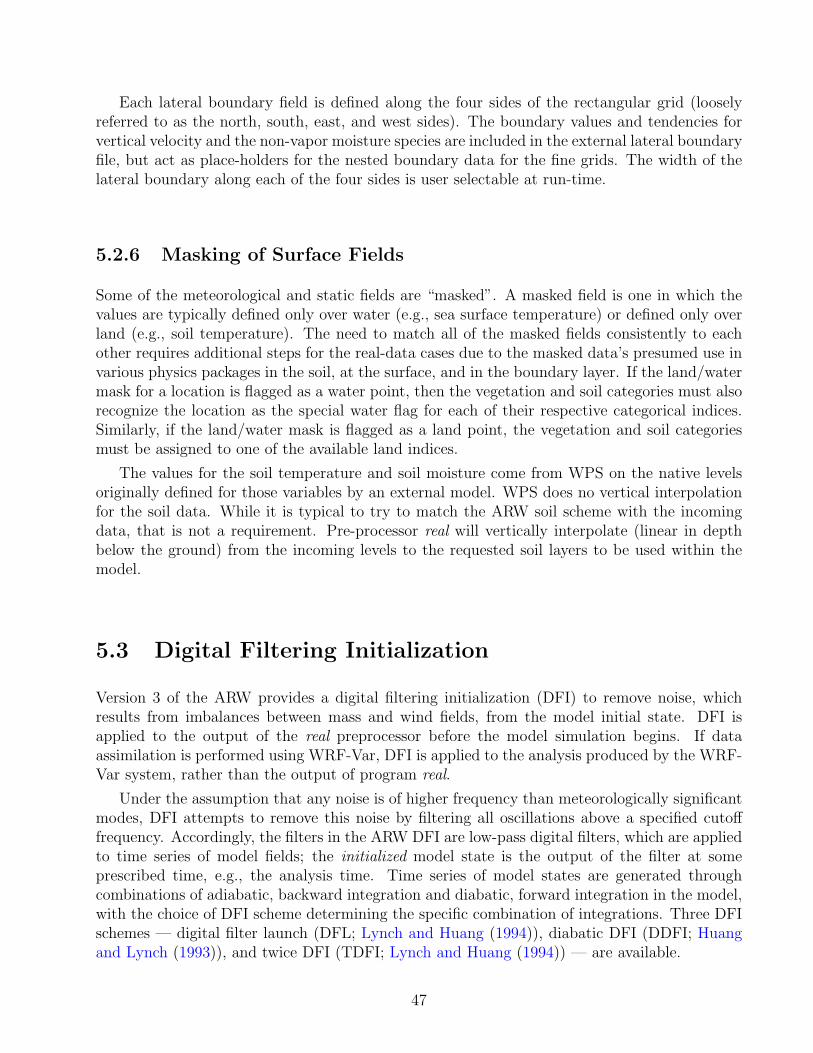
Each lateral boundary field is defined along the four sides of the rectangular grid (looselyreferred to as the north, south, east, and west sides). The boundary values and tendencies forvertical velocity and the non-vapor moisture species are included in the external lateral boundaryfile, but act as place-holders for the nested boundary data for the fine grids. The width of thelateral boundary along each of the four sides is user selectable at run-time.

5.2.6 Masking of Surface Fields

Some of the meteorological and static fields are “masked”. A masked field is one in which thevalues are typically defined only over water (e.g., sea surface temperature) or defined only overland (e.g., soil temperature). The need to match all of the masked fields consistently to eachother requires additional steps for the real-data cases due to the masked data’s presumed use invarious physics packages in the soil, at the surface, and in the boundary layer. If the land/watermask for a location is flagged as a water point, then the vegetation and soil categories must alsorecognize the location as the special water flag for each of their respective categorical indices.Similarly, if the land/water mask is flagged as a land point, the vegetation and soil categoriesmust be assigned to one of the available land indices.

The values for the soil temperature and soil moisture come from WPS on the native levelsoriginally defined for those variables by an external model. WPS does no vertical interpolationfor the soil data. While it is typical to try to match the ARW soil scheme with the incomingdata, that is not a requirement. Pre-processor real will vertically interpolate (linear in depthbelow the ground) from the incoming levels to the requested soil layers to be used within themodel.

5.3 Digital Filtering Initialization

Version 3 of the ARW provides a digital filtering initialization (DFI) to remove noise, whichresults from imbalances between mass and wind fields, from the model initial state. DFI isapplied to the output of the real preprocessor before the model simulation begins. If dataassimilation is performed using WRF-Var, DFI is applied to the analysis produced by the WRF-Var system, rather than the output of program real.

Under the assumption that any noise is of higher frequency than meteorologically significantmodes, DFI attempts to remove this noise by filtering all oscillations above a specified cutofffrequency. Accordingly, the filters in the ARW DFI are low-pass digital filters, which are appliedto time series of model fields; the initialized model state is the output of the filter at someprescribed time, e.g., the analysis time. Time series of model states are generated throughcombinations of adiabatic, backward integration and diabatic, forward integration in the model,with the choice of DFI scheme determining the specific combination of integrations. Three DFIschemes — digital filter launch (DFL; Lynch and Huang (1994)), diabatic DFI (DDFI; Huangand Lynch (1993)), and twice DFI (TDFI; Lynch and Huang (1994)) — are available.

47

5.3.1 Filter Design

In the ARW DFI, either nonrecursive (i.e., finite impulse response) digital filters or a recursive(i.e., infinite impulse response) digital filter may be used. The coefficients for the nonrecursivedigital filters may be computed according to one of two methods, while the coefficients for therecursive filter are computed according to a single method.

A general nonrecursive digital filter is of the form

yn =N

k=−N

hkxn−k, (5.10)

where yn is the output of the filter at time n, the hk are the coefficients of the filter, and. . . , xn−1, xn, xn+1, . . . is the sequence of input values to be filtered; such a filter is said to havespan 2N + 1.

One method for deriving the coefficients of a nonrecursive digital filter is the windowed-sinc method, described in the context of DFI by Lynch and Huang (1992). In the ARW DFI,either the Lanczos, Hamming, Blackman, Kaiser, Potter, or Dolph-Chebyshev windows maybe used; the Dolph-Chebyshev window is described by Lynch (1997). However, when a filterwith a shorter span is desired, another nonrecursive digital filter, the Dolph filter, may be used.Lynch (1997) describes the construction of the Dolph filter, and demonstrates that this filterhas properties nearly indistinguishable from those of an optimal filter, which minimizes themaximum difference between a filter’s transfer function and an ideal transfer function in thepass and stop bands.

The only recursive filter in the ARW DFI is the second-order Quick-Start filter of Lynch andHuang (1994). In general, a recursive digital filter that depends only on past and present valuesof the input, and on past values of the output, is of the form

yn =N

k=0

hkxn−k +N

k=1

bkyn−k. (5.11)

However, this form is inconvenient when the inputs to the filter consist of model states, andwe wish to avoid storing many such states. Lynch and Huang (1994) show how this type ofrecursive filter can be reformulated to have the same form as a nonrecursive filter, and thus, wecan think of the second-order Quick-Start filter as having the same form as (5.10).

5.3.2 DFI Schemes

The ARW supports three different DFI schemes, illustrated graphically in Fig. 5.2. The DFLscheme produces an initialized model state valid some time after the model analysis time, whilethe DDFI and TDFI schemes produce initialized states valid at the analysis time.

DFL

In the DFL scheme, forward integration with full model physics and diffusion begins at theinitial time and continues for 2N time steps, during which time a filtered model state valid N

time steps beyond the analysis time is computed as in (5.10). Then, the initialized simulation

48

t = 0

Digital Filter Launch

Diabatic DFI

Twice DFIFiltered model state

Adiabatic backward integration

Diabatic forward integration

Analysis or model initial state

Figure 5.2: An illustration showing the three available DFI schemes: digital filter launch, dia-batic digital filter initialization, and twice digital filter initialization.

is launched from the midpoint of the filtering period. For any model state X, let [X]Dn givethe model state after diabatically integrating n time steps forward in time; we emphasize thatthe superscript D indicates diabatic integration, in contrast to adiabatic integration. Then, theDFL scheme is expressed as

Xini =2N

n=0

hn [Xana]Dn , (5.12)

where Xini is the initialized model state, Xana is the model analysis or model initial stategenerated by the real preprocessor, and the hn are the filter coefficients.

DDFI

To produce an initialized state valid at the model analysis time, the DDFI scheme begins withan adiabatic, backward integration for N time steps, followed by a diabatic, forward integrationfor 2N time steps, during which filtering takes place. This filtered state is valid at the modelanalysis time. Letting [Xana]

A−n denote the model state after adiabatic, backward integration for

n time steps from the model analysis or model initial state, Xana, the DDFI scheme is expressedas

Xini =2N

n=0

hn

[Xana]

A−n

D

n, (5.13)

where Xini is the initialized model state valid at the model analysis time.

TDFI

The TDFI scheme involves two applications of the digital filter. Adiabatic, backward integrationproceeds from the model initial time for 2N time steps, during which a filter is applied. Thefiltered state is valid at time −N∆t; from this filtered state, a forward, diabatic integration is

49

launched. The second integration proceeds for 2N time steps, during which a second filter isapplied, giving a filtered model state valid at this model analysis time. The TDFI scheme isexpressed as

Xini =2N

n=0

hn

2N

n=0

hn [Xana]A−n

D

n

. (5.14)

5.3.3 Backward Integration

To diabatically integrate backward in time, it suffices to disable all diabatic processes and tonegate the model time step, ∆t, as well as the sign of the horizontal velocity, U , in the odd-orderadvection operators of Section 3.2.3, which become

3rd order: (qxadv)i−1/2 = (qxadv)4th

i−1/2

− sign(U)1

12

(qi+1 − qi−2)− 3(qi − qi−1)

5th order: (qxadv)i−1/2 = (qxadv)6th

i−1/2

+ sign(U)1

60

(qi+2 − qi−3)− 5(qi+1 − qi−2) + 10(qi − qi−1)

.

When specified boundary conditions are used, as in Section 6.4, the model boundaries beforethe model initial time are taken to be the same as those valid at the model initial time. We notethat, with a negated time step, the linear ramping functions F1 and F2 of (6.1) change sign,and, consequently, so does the sign of the tendency for a prognostic variable ψ.

50

Chapter 6

Lateral Boundary Conditions

Several lateral boundary condition options exist for the ARW that are suitable for idealized flows,and a specified lateral boundary condition for real-data simulations is available. These choicesare handled via a run-time option in the Fortran namelist file. For nesting, all fine domainsuse the nest time-dependent lateral boundary condition where the outer row and column of thefine grid is specified from the parent domain, described in Section 7.3. The remaining lateralboundary options are exclusively for use by the most coarse/parent domain.

6.1 Periodic Lateral Boundary Conditions

Periodic lateral boundary conditions in the ARW can be specified as periodic in x (west-east),y (south-north), or doubly periodic in (x, y). The periodic boundary conditions constrain thesolutions to be periodic; that is, a generic model state variable ψ will follow the relation

ψ(x + nLx, y + mLy) = ψ(x, y)

for all integer (n, m). The periodicity lengths (Lx, Ly) are[(dimension of the domain in x) - 1]∆x and [(dimension of the domain in y) - 1]∆y.

6.2 Open Lateral Boundary Conditions

Open lateral boundary conditions, also referred to as gravity-wave radiating boundary condi-tions, can be specified for the west, east, north, or south boundary, or any combination thereof.The gravity wave radiation conditions follow the approach of Klemp and Lilly (1978) and Klempand Wilhelmson (1978).

There are a number of changes in the base numerical algorithm described in Chapter 3 thataccompany the imposition of these conditions. First, for the normal horizontal velocities alonga boundary on which the condition is specified, the momentum equation for the horizontalvelocity, (3.7) or (3.8), is replaced by

δτU = −U

∗δxu,

where U∗ = min(U − cb, 0) at the x = 0 (western) boundary, U

∗ = max(U + cb, 0) at the x = L

(eastern) boundary, and likewise for the south and north boundaries for the V momentum. The

51

horizontal difference operator δx is evaluated in a one-sided manner using the difference betweenthe boundary value and the value one grid-point into the grid from the boundary. cb is the phasespeed of the gravity waves that are to be radiated; it is specified as a model constant (for moredetails see Klemp and Lilly, 1978; Klemp and Wilhelmson, 1978).

For scalars and non-normal momentum variables, the boundary-perpendicular flux diver-gence term is replaced with

δx(Uψ) = U∗δxψ + ψ δxU,

where U∗ = min(U, 0) at the x = 0 + ∆x/2 (western) scalar boundary, U

∗ = max(U, 0) at thex = L−∆x/2 (eastern) boundary, and likewise for the south and north boundaries using V . Aswas the case for the momentum equations, the horizontal difference operator δx is evaluated in aone-sided manner using the difference between the boundary value and the value one grid-pointinto the grid from the boundary.

6.3 Symmetric Lateral Boundary Conditions

Symmetry lateral boundary conditions can be specified for the west, east, north, or south bound-ary, or any combination thereof. The symmetry boundaries are located on the normal-velocityplanes at the lateral edges of the grids. The normal velocities are zero at these boundaries, andon either side of the boundary the normal velocity satisfies the relation

U⊥(xb − x) = −U⊥(xb + x),

where xb is the location of the symmetry boundary. All other variables satisfy the relation

ψ(xb − x) = ψ(xb + x).

6.4 Specified Lateral Boundary Conditions

Primarily for real-data cases, the specified boundary condition is also referred to as a relaxation,or nudging, boundary condition. There are two uses of the specified boundaries in the ARW:for the outer-most coarse grid or for the time-dependent boundaries supplied to a nested grid.The specified lateral boundary conditions for the nest are automatically selected for all of thefine grids, even if the coarse grid is using combinations of the symmetry, periodic, or openoptions. If the specified lateral boundary condition is selected for the coarse grid, then all fourgrid sides (west, east, north, and south) use specified lateral conditions. However, in tropicalchannel mode, where the domain wraps completely around the equator, it is possible to combinespecified boundary conditions with periodic conditions in the x direction. Note that care isneeded in setting the domain up such that the points exactly match longitude at the east andwest boundaries when periodic conditions are used in real-data cases. Also note that a Mercatorprojection is needed to make this possible.

The coarse grid specified lateral boundary is comprised of both a specified and a relaxationzone (as shown in Fig. 6.1). For the coarse grid, the specified zone is determined entirely bytemporal interpolation from an external forecast or analysis (supplied by WPS). The width ofthe specified zone is run-time configurable, but is typically set to 1 (i.e., the last row and column

52

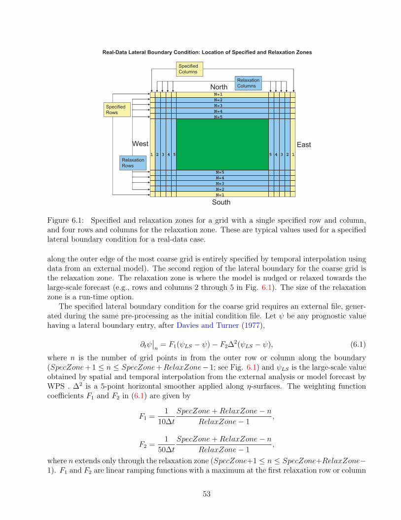
RelaxationRows

South

EastWest

NorthN=1N=2N=3N=4N=5

N=5N=4N=3N=2N=1

1 2 3 4 5 5 4 3 2 1

RelaxationColumns

SpecifiedColumns

SpecifiedRows

Real-Data Lateral Boundary Condition: Location of Specified and Relaxation Zones

Figure 6.1: Specified and relaxation zones for a grid with a single specified row and column,and four rows and columns for the relaxation zone. These are typical values used for a specifiedlateral boundary condition for a real-data case.

along the outer edge of the most coarse grid is entirely specified by temporal interpolation usingdata from an external model). The second region of the lateral boundary for the coarse grid isthe relaxation zone. The relaxation zone is where the model is nudged or relaxed towards thelarge-scale forecast (e.g., rows and columns 2 through 5 in Fig. 6.1). The size of the relaxationzone is a run-time option.

The specified lateral boundary condition for the coarse grid requires an external file, gener-ated during the same pre-processing as the initial condition file. Let ψ be any prognostic valuehaving a lateral boundary entry, after Davies and Turner (1977),

∂tψn

= F1(ψLS − ψ)− F2∆2(ψLS − ψ), (6.1)

where n is the number of grid points in from the outer row or column along the boundary(SpecZone+1 ≤ n ≤ SpecZone+RelaxZone− 1; see Fig. 6.1) and ψLS is the large-scale valueobtained by spatial and temporal interpolation from the external analysis or model forecast byWPS . ∆2 is a 5-point horizontal smoother applied along η-surfaces. The weighting functioncoefficients F1 and F2 in (6.1) are given by

F1 =1

10∆t

SpecZone + RelaxZone− n

RelaxZone− 1,

F2 =1

50∆t


RelaxZone− 1,

where n extends only through the relaxation zone (SpecZone+1 ≤ n ≤ SpecZone+RelaxZone−1). F1 and F2 are linear ramping functions with a maximum at the first relaxation row or column

53

nearest the coarse grid boundary (just inside of the specified zone). In Version 3.0 these linearfunctions can optionally be multiplied by an exponential function for smoother behavior whenbroad boundary zones are needed. This is achieved through an additional multiplier.

F1 =1

10∆t


RelaxZone− 1exp[−SpecExp(n− SpecZone− 1)]

F2 =1

50∆t


RelaxZone− 1exp[−SpecExp(n− SpecZone− 1)]

where SpecExp is an inverse length scale in grid lengths.On the coarse grid, the specified boundary condition applies to the horizontal wind com-

ponents, potential temperature, φ, µ

d, and water vapor. The lateral boundary file contains

enough information to update the boundary zone values through the entire simulation period.The momentum fields are coupled with µd and the inverse map factor (both at the specificvariable’s horizontal staggering location), and the other 3-dimensional fields are coupled withµd. The µ

d field is not coupled in the lateral boundary file.

Vertical velocity has a zero gradient boundary condition applied in the specified zone (usuallythe outer-most row and column). Microphysical variables, except vapor, and all other scalarshave flow-dependent boundary conditions applied in the specified zone. This boundary conditionspecifies zero on inflow and zero-gradient on outflow. Since these boundary conditions requireonly information from the interior of the grid, these variables are not in the specified boundarycondition file. However, for nested boundaries, microphysical variables and scalars are alsoavailable from the parent domain, and use same relaxation towards interpolated variables as thedynamic variables.

6.5 Polar Conditions

See subsection 3.2.4 for details on how the polar boundary condition is applied.

54

Chapter 7

Nesting

The ARW supports horizontal nesting that allows resolution to be focused over a region ofinterest by introducing an additional grid (or grids) into the simulation. In the current im-plementation, only horizontal refinement is available: there is no vertical nesting option. Thenested grids are rectangular and are aligned with the parent (coarser) grid within which they arenested. Additionally, the nested grids allow any integer spatial (∆xcoarse/∆xfine) and temporalrefinements of the parent grid (the spatial and temporal refinements are usually, but not neces-sarily the same). This nesting implementation is in many ways similar to the implementations inother mesoscale and cloudscale models (e.g. MM5, ARPS, COAMPS). The major improvementin the ARW’s nesting infrastruture compared with techniques used in other models is the abil-ity to compute nested simulations efficiently on parallel distributed-memory computer systems,which includes support for moving nested grids. The WRF Software Framework, described inMichalakes et al. (2004), makes these advances possible. In this chapter we describe the variousnesting options available in the ARW and the numerical coupling between the grids.

7.1 Nesting Options

1-Way and 2-Way Grid Nesting

Nested grid simulations can be produced using either 1-way nesting or 2-way nesting as outlinedin Fig. 7.1. The 1-way and 2-way nesting options refer to how a coarse grid and the fine gridinteract. In both the 1-way and 2-way simulation modes, the fine grid boundary conditions (i.e.,the lateral boundaries) are interpolated from the coarse grid forecast. In a 1-way nest, this is theonly information exchange between the grids (from the coarse grid to the fine grid). Hence, thename 1-way nesting. In the 2-way nest integration, the fine grid solution replaces the coarse gridsolution for coarse grid points that lie inside the fine grid. This information exchange betweenthe grids is now in both directions (coarse-to-fine for the fine-grid lateral boundary computationand fine-to-coarse during the feedback at each coarse-grid time step). Hence, the name 2-waynesting.

The 1-way nest set-up may be run in one of two different methods. One option is to producethe nested simulation as two separate ARW simulations as described in the leftmost box in Fig.7.1. In this mode, the coarse grid is integrated first and the coarse grid forecast is completed.Output from the coarse grid integration is then processed to provide boundary conditions forthe nested run (usually at a much lower temporal frequency than the coarse grid time step), and

55

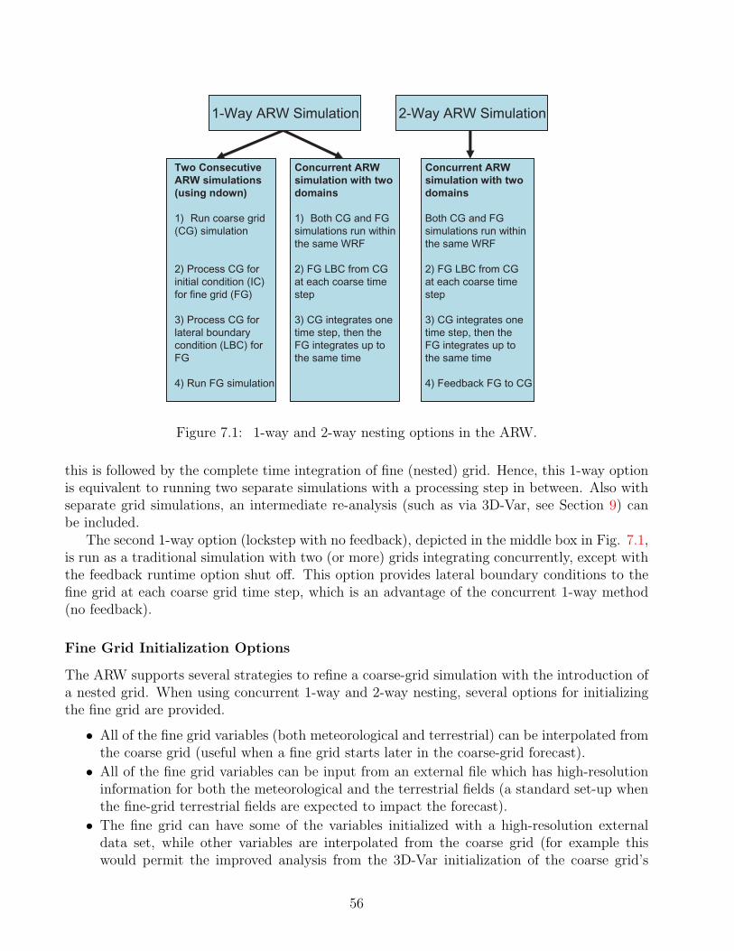
Concurrent ARWsimulation with twodomains

Both CG and FGsimulations run withinthe same WRF

2) FG LBC from CGat each coarse timestep

3) CG integrates onetime step, then the FG integrates up tothe same time

4) Feedback FG to CG

2-Way ARW Simulation

Two ConsecutiveARW simulations(using ndown)

1) Run coarse grid(CG) simulation

2) Process CG forinitial condition (IC)for fine grid (FG)

3) Process CG forlateral boundarycondition (LBC) forFG

4) Run FG simulation

Concurrent ARW simulation with twodomains

1) Both CG and FGsimulations run withinthe same WRF

2) FG LBC from CGat each coarse timestep

3) CG integrates onetime step, then the FG integrates up tothe same time

1-Way WRF Simulation1-Way ARW Simulation

Figure 7.1: 1-way and 2-way nesting options in the ARW.

this is followed by the complete time integration of fine (nested) grid. Hence, this 1-way optionis equivalent to running two separate simulations with a processing step in between. Also withseparate grid simulations, an intermediate re-analysis (such as via 3D-Var, see Section 9) canbe included.

The second 1-way option (lockstep with no feedback), depicted in the middle box in Fig. 7.1,is run as a traditional simulation with two (or more) grids integrating concurrently, except withthe feedback runtime option shut off. This option provides lateral boundary conditions to thefine grid at each coarse grid time step, which is an advantage of the concurrent 1-way method(no feedback).

Fine Grid Initialization Options

The ARW supports several strategies to refine a coarse-grid simulation with the introduction ofa nested grid. When using concurrent 1-way and 2-way nesting, several options for initializingthe fine grid are provided.

• All of the fine grid variables (both meteorological and terrestrial) can be interpolated fromthe coarse grid (useful when a fine grid starts later in the coarse-grid forecast).

• All of the fine grid variables can be input from an external file which has high-resolutioninformation for both the meteorological and the terrestrial fields (a standard set-up whenthe fine-grid terrestrial fields are expected to impact the forecast).

• The fine grid can have some of the variables initialized with a high-resolution externaldata set, while other variables are interpolated from the coarse grid (for example thiswould permit the improved analysis from the 3D-Var initialization of the coarse grid’s

56

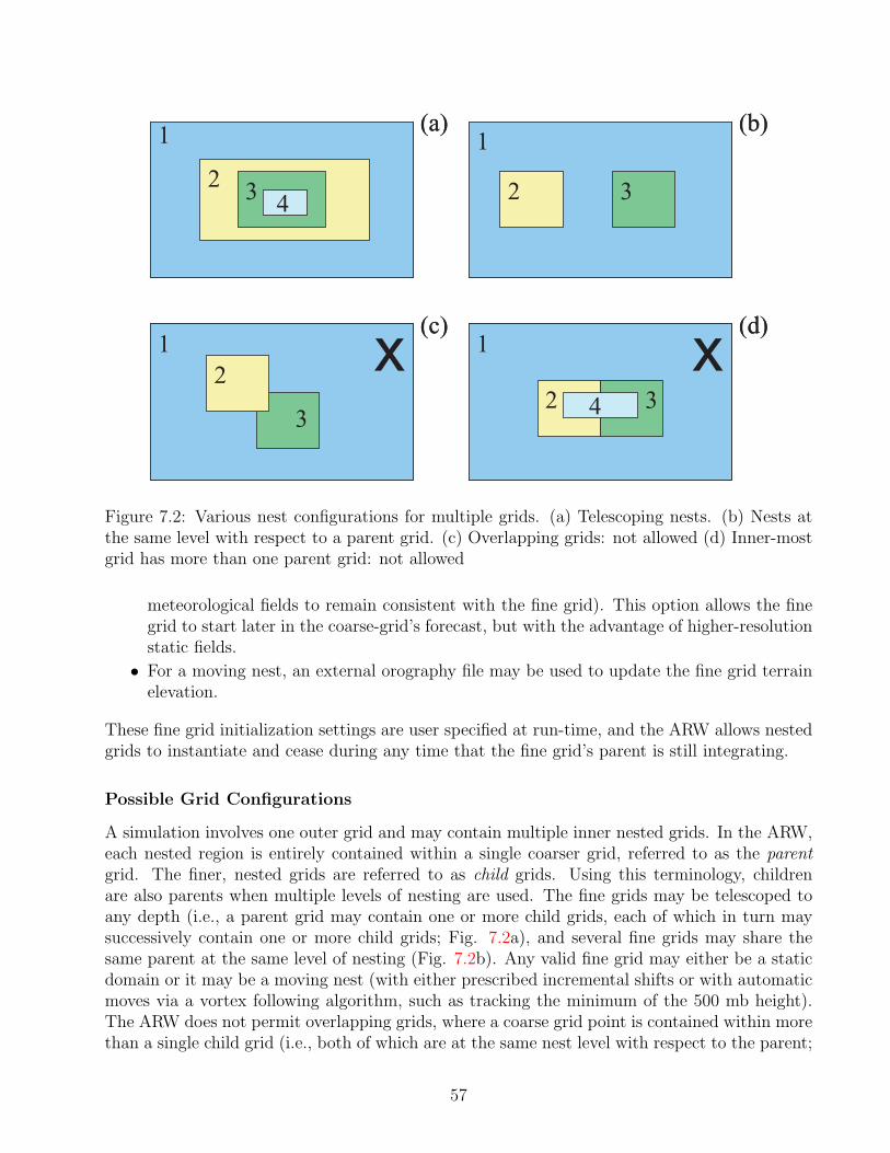
(c)1

2

3

(c)1

2

3

(b)1

2 3

(b)1

2 3

(a)1

2 3 4

(a)1

2 3 4

(d)1

2 34

(d)1

2 34

x x

Figure 7.2: Various nest configurations for multiple grids. (a) Telescoping nests. (b) Nests atthe same level with respect to a parent grid. (c) Overlapping grids: not allowed (d) Inner-mostgrid has more than one parent grid: not allowed

meteorological fields to remain consistent with the fine grid). This option allows the finegrid to start later in the coarse-grid’s forecast, but with the advantage of higher-resolutionstatic fields.

• For a moving nest, an external orography file may be used to update the fine grid terrainelevation.

These fine grid initialization settings are user specified at run-time, and the ARW allows nestedgrids to instantiate and cease during any time that the fine grid’s parent is still integrating.

Possible Grid Configurations

A simulation involves one outer grid and may contain multiple inner nested grids. In the ARW,each nested region is entirely contained within a single coarser grid, referred to as the parentgrid. The finer, nested grids are referred to as child grids. Using this terminology, childrenare also parents when multiple levels of nesting are used. The fine grids may be telescoped toany depth (i.e., a parent grid may contain one or more child grids, each of which in turn maysuccessively contain one or more child grids; Fig. 7.2a), and several fine grids may share thesame parent at the same level of nesting (Fig. 7.2b). Any valid fine grid may either be a staticdomain or it may be a moving nest (with either prescribed incremental shifts or with automaticmoves via a vortex following algorithm, such as tracking the minimum of the 500 mb height).The ARW does not permit overlapping grids, where a coarse grid point is contained within morethan a single child grid (i.e., both of which are at the same nest level with respect to the parent;

57

Fig. 7.2c). In addition, no grid can have more than a single parent (Fig. 7.2d). For globaldomains, a fine grid domain cannot cross the periodic lateral boundary of the parent domain.

For both 1-way and 2-way nested grid simulations, the ratio of the parent horizontal griddistance to the child horizontal grid distance (the spatial refinement ratio) must be an integer.For 2-way and concurrent 1-way nesting, this is also true for the time steps (the temporalrefinement ratio). The model does allow the time step refinement ratio to differ from the spatialrefinement ratio. Also, nested grids on the same level (i.e., children who have the same parent)may have different spatial and temporal refinement ratios. For example, in Fig. 7.2b, thehorizontal grid resolution for domain 1 could be 90 km, for domain 2 could be 45 km, and fordomain 3 could be 30 km.

Moving Nests

The moving nest capabilities in ARW are simply extensions to the suite of nesting options. Alldescriptions covering the specifics for the fine-grid domains (initialization, feedback, configura-tions, staggering, lateral boundaries, etc.) apply also to moving nests. In general, all nests inan ARW forecast are eligible to be moving nests. The ARW provides two methods to have nestsmove during the model integration: specified and automatic.

For a specified move, the timing of a nest move and the extent of the lateral move is definedentirely by the user. For the automatically moving nest, the fine grid is initialized to cover awell defined vortex, and the nest moves to maintain this vortex in the center of the fine grid.For both types of moving nests, multiple levels of domains may move. However, most of theinstances where a moving nest is utilized are during tropical cyclone tracking via the vortexfollowing technique.

After a nested domain has moved a parent grid-cell distance, the majority of the data in thedomain is still valid. The data that is not along the outer row or column of the nested domainis shifted to the new location in that domain. Once a domain moves, the data in the outerrow or column falls into two categories: discarded data on the trailing edge, and horizontallyinterpolated data on the leading edge in the direction of the nest move.

7.2 Staggering and Feedback

The ARW uses an Arakawa-C grid staggering. As shown in Fig. 7.3, the u and v com-ponents of horizontal velocity are normal to the respective faces of the grid cell, and themass/thermodynamic/scalar/chemistry variables are located in the center of the cell.

The variable staggering has an additional column of u in the x-direction and an addi-tional row of v in the y-direction because the normal velocity points define the grid bound-aries. The horizontal momentum components reflect an average across each cell-face, while eachmass/thermodynamic/scalar/chemistry variable is the representative mean value throughout thecell. Feedback is handled to preserve these mean values: the mass/thermodynamic/scalar/chemistryfields are fed back with an average from within the entire coarse grid point (Fig. 7.3), and thehorizontal momentum variables are averaged along their respective normal coarse grid cell faces.

The horizontal interpolation (to instantiate a grid and to provide time-dependent lateralboundaries) does not conserve mass. The feedback mechanism, for most of the unmasked fields,

58

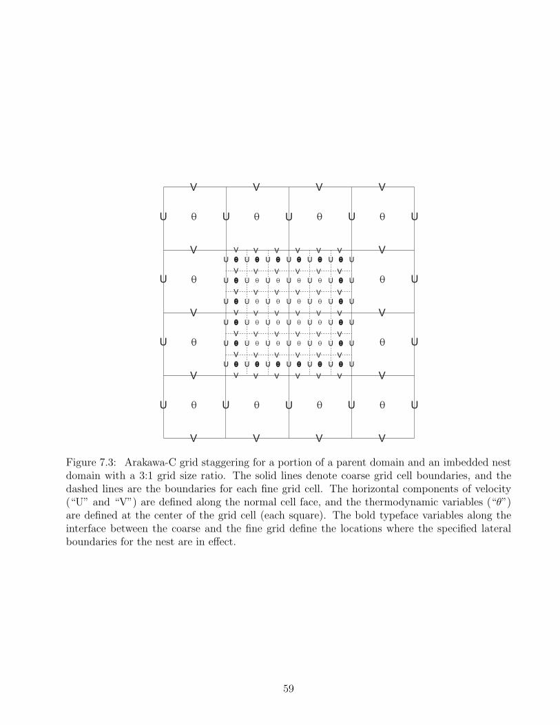
U UU U U UU

U UU U U UU

U UU U U UU

U UU U U UU

U UU U U UU

U UU U U UU

VV V V V V

VV V V V V

VV V V V V

VV V V V V

VV V V V V

VV V V V V

VV V V V V

U U U U U

U U

U U

U U U U U

V V V V

V V

V V

V V

V V V V

Figure 7.3: Arakawa-C grid staggering for a portion of a parent domain and an imbedded nestdomain with a 3:1 grid size ratio. The solid lines denote coarse grid cell boundaries, and thedashed lines are the boundaries for each fine grid cell. The horizontal components of velocity(“U” and “V”) are defined along the normal cell face, and the thermodynamic variables (“θ”)are defined at the center of the grid cell (each square). The bold typeface variables along theinterface between the coarse and the fine grid define the locations where the specified lateralboundaries for the nest are in effect.

59

uses cell averages (for mass/thermodynamic/scalar/chemistry quantities) and cell-face averagesfor the horizontal momentum fields.

The staggering defines the way that the fine grid is situated on top of the coarse grid. For allodd ratios there is a coincident point for each variable: a location that has the coarse grid andthe fine grid at the same physical point. The location of this point depends on the variable. Ineach of the coarse-grid cells with an odd ratio, the middle fine-grid cell is the coincident pointwith the coarse grid for all of the mass-staggered fields (Fig. 7.3). For the horizontal momentumvariables the normal velocity has coincident points along the grid boundaries for odd ratios.

For fields that are averaged back to the coarse grid in the feedback, the mean of the ninemass/thermodynamic/scalar/chemistry (for example, due to the 3:1 grid-distance ratio in theexample shown in Fig. 7.3) fine grid points is fed back to the coarse grid. These fields includemost 3-dimensional and 2-dimensional arrays. For the horizontal momentum fields averaged backto the coarse grid in the feedback, the mean of three (for example, due to the 3:1 grid-distanceratio in the example shown in Fig. 7.3) fine grid points is fed back to the coarse grid from alongthe coincident cell face. The fields that are masked due to the land/sea category are fed backdirectly from the coincident points for odd ratios. Masked fields include soil temperature andsea ice. It does not make sense to average neighboring locations of soil temperature on the finegrid if the coarse grid point being fedback to is a water value. Similarly, averaging several seaice values on the fine grid does not make sense if some of the neighboring points included inthe mean are fine grid land points. Only masked fields use the feedback method where a singlepoint from the fine grid is assigned to the coarse grid.

A difference between the odd and even grid-distance ratios is in the feedback from the finegrid to the coarse grid. No coincident points exist for the single point feedback mechanismsfor even grid distance ratios (such as used for the land/sea masked 2D fields). For a 2:1 evengrid distance ratio, Figure 7.4 shows that each coarse grid point has four fine grid cells thatare equally close, and therefore four equally eligible grid points for use as the single fine-gridpoint that feeds back to the coarse grid. The single-point feedback is arbitrarily chosen as thesouth-west corner of the four neighboring points. This arbitrary assignment to masked fieldsimplies that even grid distance ratios are more suited for idealized simulations where maskedfields are less important.

7.3 Nested Lateral Boundary Conditions

For the fine grid with 2-way nesting or 1-way nesting (using a concurrent ARW simulation,see Fig. 7.1), the boundary conditions are specified by the parent grid at every coarse-gridtime step. The nest lateral boundary condition behaves similarly to the specified boundarycondition for real-data cases (see Section 6.4), but the relaxation zone is not active. Prognosticvariables are entirely specified in the outer row and column of the fine grid through spatial andtemporal interpolation from the coarse grid (the coarse grid is stepped forward in time prior toadvancement of any child grid of that parent).

60

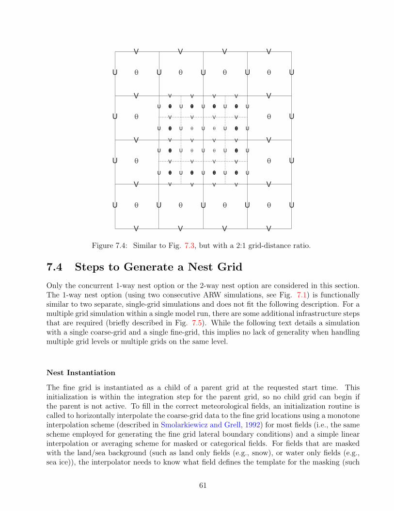
U UU U U

U UU U U

U UU U U

U UU U U

V V V V

V V V V

V V V V

V V V V

V V V V

U U U U U

U U

U U

U U U U U

V V V V

V V

V V

V V

V V V V

Figure 7.4: Similar to Fig. 7.3, but with a 2:1 grid-distance ratio.

7.4 Steps to Generate a Nest Grid

Only the concurrent 1-way nest option or the 2-way nest option are considered in this section.The 1-way nest option (using two consecutive ARW simulations, see Fig. 7.1) is functionallysimilar to two separate, single-grid simulations and does not fit the following description. For amultiple grid simulation within a single model run, there are some additional infrastructure stepsthat are required (briefly described in Fig. 7.5). While the following text details a simulationwith a single coarse-grid and a single fine-grid, this implies no lack of generality when handlingmultiple grid levels or multiple grids on the same level.

Nest Instantiation

The fine grid is instantiated as a child of a parent grid at the requested start time. Thisinitialization is within the integration step for the parent grid, so no child grid can begin ifthe parent is not active. To fill in the correct meteorological fields, an initialization routine iscalled to horizontally interpolate the coarse-grid data to the fine grid locations using a monotoneinterpolation scheme (described in Smolarkiewicz and Grell, 1992) for most fields (i.e., the samescheme employed for generating the fine grid lateral boundary conditions) and a simple linearinterpolation or averaging scheme for masked or categorical fields. For fields that are maskedwith the land/sea background (such as land only fields (e.g., snow), or water only fields (e.g.,sea ice)), the interpolator needs to know what field defines the template for the masking (such

61

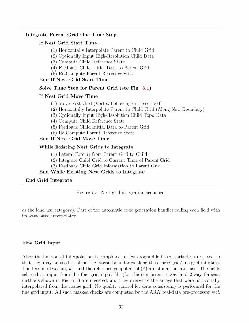
Integrate Parent Grid One Time Step

If Nest Grid Start Time

(1) Horizontally Interpolate Parent to Child Grid(2) Optionally Input High-Resolution Child Data(3) Compute Child Reference State(4) Feedback Child Initial Data to Parent Grid(5) Re-Compute Parent Reference State

End If Nest Grid Start Time

Solve Time Step for Parent Grid (see Fig. 3.1)

If Nest Grid Move Time

(1) Move Nest Grid (Vortex Following or Prescribed)(2) Horizontally Interpolate Parent to Child Grid (Along New Boundary)(3) Optionally Input High-Resolution Child Topo Data(4) Compute Child Reference State(5) Feedback Child Initial Data to Parent Grid(6) Re-Compute Parent Reference State

End If Nest Grid Move Time

While Existing Nest Grids to Integrate

(1) Lateral Forcing from Parent Grid to Child(2) Integrate Child Grid to Current Time of Parent Grid(3) Feedback Child Grid Information to Parent Grid

End While Existing Nest Grids to Integrate

End Grid Integrate

Figure 7.5: Nest grid integration sequence.

as the land use category). Part of the automatic code generation handles calling each field withits associated interpolator.

Fine Grid Input

After the horizontal interpolation is completed, a few orographic-based variables are saved sothat they may be used to blend the lateral boundaries along the coarse-grid/fine-grid interface.The terrain elevation, µd, and the reference geopotential (φ) are stored for later use. The fieldsselected as input from the fine grid input file (for the concurrent 1-way and 2-way forecastmethods shown in Fig. 7.1) are ingested, and they overwrite the arrays that were horizontallyinterpolated from the coarse grid. No quality control for data consistency is performed for thefine grid input. All such masked checks are completed by the ARW real-data pre-processor real.

62

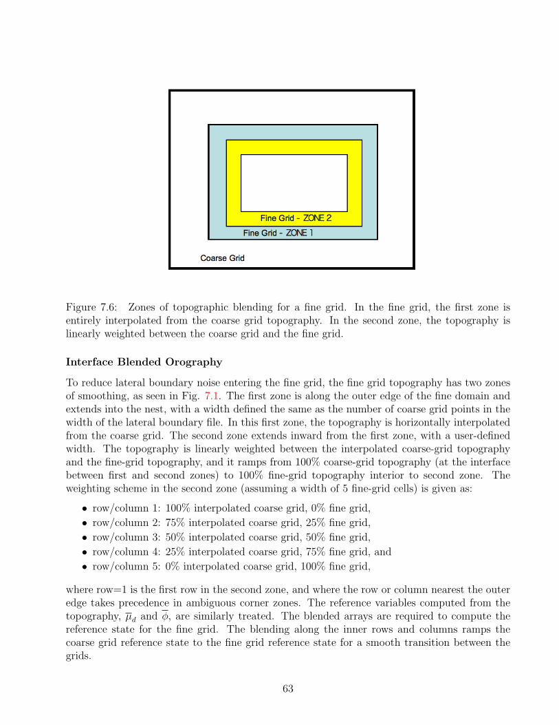
Figure 7.6: Zones of topographic blending for a fine grid. In the fine grid, the first zone isentirely interpolated from the coarse grid topography. In the second zone, the topography islinearly weighted between the coarse grid and the fine grid.

Interface Blended Orography

To reduce lateral boundary noise entering the fine grid, the fine grid topography has two zonesof smoothing, as seen in Fig. 7.1. The first zone is along the outer edge of the fine domain andextends into the nest, with a width defined the same as the number of coarse grid points in thewidth of the lateral boundary file. In this first zone, the topography is horizontally interpolatedfrom the coarse grid. The second zone extends inward from the first zone, with a user-definedwidth. The topography is linearly weighted between the interpolated coarse-grid topographyand the fine-grid topography, and it ramps from 100% coarse-grid topography (at the interfacebetween first and second zones) to 100% fine-grid topography interior to second zone. Theweighting scheme in the second zone (assuming a width of 5 fine-grid cells) is given as:

• row/column 1: 100% interpolated coarse grid, 0% fine grid,



• row/column 4: 25% interpolated coarse grid, 75% fine grid, and


where row=1 is the first row in the second zone, and where the row or column nearest the outeredge takes precedence in ambiguous corner zones. The reference variables computed from thetopography, µd and φ, are similarly treated. The blended arrays are required to compute thereference state for the fine grid. The blending along the inner rows and columns ramps thecoarse grid reference state to the fine grid reference state for a smooth transition between thegrids.

63

Feedback

So that the coarse grid and the fine grid are consistent at coincident points, the fine grid valuesare fed back to the coarse grid. There are two available options for feedback: either the mean ofall fine grid cells contained within each coarse grid cell is fed back (or cell faces in the case of thehorizontal momentum fields), or a single-point feedback is selected for the masked or categoricalfields.

Subsequent to the feedback step, the coarse grid may be optionally smoothed in the area ofthe fine grid. Two smoothers are available: a 5-point 1-2-1 smoother and a smoother-desmootherwith a similar stencil size. Both the feedback and the smoothers are run one row and columnin from the interface row and column of the coarse grid that provides the lateral boundaryconditions to the fine grid.

Reference State

The initial feedback when the nest is instantiated ensures that the coarse grid is consistentwith the fine grid, particularly with regards to elevation and the reference state fields inside theblended region, and for such terrestrial features as coasts, lakes, and islands. The adjustment ofthe elevation in the coarse grid forces a base state recalculation. The fine-grid needs an initialbase state calculation, and after the terrain feedback, the coarse grid is also in need of a basestate recalculation.

Note that with the horizontal interpolation of the coarse grid to the fine grid and the feedbackof the fine grid to the coarse grid, the coarse grid base state is recomputed even without a separatefine-grid initial data file, since the coarse grid topography is adjusted.

With the completed base state computations, which follow similarly to that described forthe real-data initialization in section 5.2.2, the routines return back to the integration step forthe coarse and fine grids. The fine grid data is now properly initialized for integration and canbe advanced forward a time step.

Integration

The integration by grid is recursive. At the end of each grid’s time step, a check is made todetermine if a child grid exists for that parent and if the current time is bracketed by the child’sstart/end time. This is shown in Fig. 7.5. The integration process for the nest (step 2 underthe while loop) is recursively calling the top step in the overall sequence as a coarse grid itself.This is a “depth first” traversal of the tree of grids. If a child grid does exist, that child grid isintegrated up through the current time of the parent grid.

64

Chapter 8

Physics

This chapter outlines the physics options available in the ARW. The WRF physics options fallinto several categories, each containing several choices. The physics categories are (1) micro-physics, (2) cumulus parameterization, (3) planetary boundary layer (PBL), (4) land-surfacemodel, and (5) radiation. Diffusion, which may also be considered part of the physics, is de-scribed in Chapter 4. The chapter will also address four-dimensional data assimilation (FDDA)methods that are available in ARW. These methods apply extra forcings to the model equations,and are internally treated similarly to physics.

The physics section is insulated from the rest of the dynamics solver by the use of physicsdrivers. These are between solver-dependent routines: a pre-physics preparation and post-physics modifications of the tendencies. The physics preparation involves filling arrays withphysics-required variables that include the temperature, pressure, heights, layer thicknesses,and other state variables in MKS units at half-level grid points and on full levels. The velocitiesare also de-staggered so that the physics part is independent of the dynamical solver’s velocitystaggering. Physics packages compute tendencies for the velocity components (un-staggered),potential temperature, and moisture fields. The solver-dependent post-physics step will re-stagger these tendencies as necessary, couple tendencies with coordinate metrics, and convert tovariables or units appropriate to the dynamics solver.

In the first Runge-Kutta step, prior to the acoustic steps (see Fig. 3.1, step(1)), tendenciesare computed for radiation, surface, PBL, and cumulus physics. These tendencies are then heldfixed through the Runge-Kutta steps. Microphysics is computed after the last Runge-Kuttastep (see Fig. 3.1, step (9)) in order to maintain proper saturation conditions at the end of thetime-step.

The initialization of the physics is called prior to the first model step. This initializationmay include reading in data files for physics tables or calculating look-up tables of functions.Each physics module includes an initialization routine for this purpose. Often physics packageswill have many of their own constants that should also be included in their own module, whilecommon physical constants are passed in from the physics drivers.

8.1 Microphysics

Microphysics includes explicitly resolved water vapor, cloud, and precipitation processes. Themodel is general enough to accommodate any number of mass mixing-ratio variables, and other

65

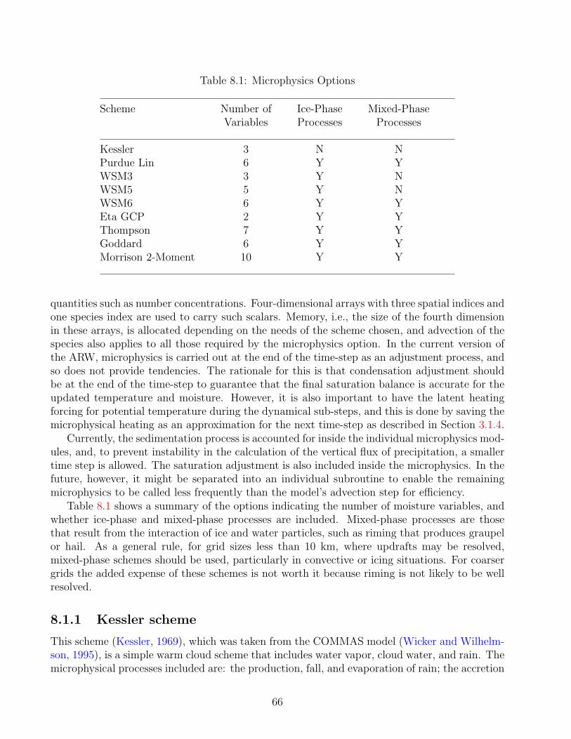
Table 8.1: Microphysics Options

Scheme Number of Ice-Phase Mixed-PhaseVariables Processes Processes

Kessler 3 N NPurdue Lin 6 Y YWSM3 3 Y NWSM5 5 Y NWSM6 6 Y YEta GCP 2 Y YThompson 7 Y YGoddard 6 Y YMorrison 2-Moment 10 Y Y

quantities such as number concentrations. Four-dimensional arrays with three spatial indices andone species index are used to carry such scalars. Memory, i.e., the size of the fourth dimensionin these arrays, is allocated depending on the needs of the scheme chosen, and advection of thespecies also applies to all those required by the microphysics option. In the current version ofthe ARW, microphysics is carried out at the end of the time-step as an adjustment process, andso does not provide tendencies. The rationale for this is that condensation adjustment shouldbe at the end of the time-step to guarantee that the final saturation balance is accurate for theupdated temperature and moisture. However, it is also important to have the latent heatingforcing for potential temperature during the dynamical sub-steps, and this is done by saving themicrophysical heating as an approximation for the next time-step as described in Section 3.1.4.

Currently, the sedimentation process is accounted for inside the individual microphysics mod-ules, and, to prevent instability in the calculation of the vertical flux of precipitation, a smallertime step is allowed. The saturation adjustment is also included inside the microphysics. In thefuture, however, it might be separated into an individual subroutine to enable the remainingmicrophysics to be called less frequently than the model’s advection step for efficiency.

Table 8.1 shows a summary of the options indicating the number of moisture variables, andwhether ice-phase and mixed-phase processes are included. Mixed-phase processes are thosethat result from the interaction of ice and water particles, such as riming that produces graupelor hail. As a general rule, for grid sizes less than 10 km, where updrafts may be resolved,mixed-phase schemes should be used, particularly in convective or icing situations. For coarsergrids the added expense of these schemes is not worth it because riming is not likely to be wellresolved.

8.1.1 Kessler scheme

This scheme (Kessler, 1969), which was taken from the COMMAS model (Wicker and Wilhelm-son, 1995), is a simple warm cloud scheme that includes water vapor, cloud water, and rain. Themicrophysical processes included are: the production, fall, and evaporation of rain; the accretion

66

and autoconversion of cloud water; and the production of cloud water from condensation.

8.1.2 Purdue Lin scheme

Six classes of hydrometeors are included: water vapor, cloud water, rain, cloud ice, snow, andgraupel. All parameterization production terms are based on Lin et al. (1983) and Rutledgeand Hobbs (1984) with some modifications, including saturation adjustment following Tao et al.(1989) and ice sedimentation. This is a relatively sophisticated microphysics scheme in WRF,and it is most suitable for use in research studies. The scheme is taken from the Purdue cloudmodel, and the details can be found in Chen and Sun (2002).

8.1.3 WRF Single-Moment 3-class (WSM3) scheme

The WRF single-moment microphysics scheme follows Hong et al. (2004) including ice sedimen-tation and other new ice-phase parameterizations. A major difference from other approaches isthat a diagnostic relation is used for ice number concentration that is based on ice mass contentrather than temperature. The computational procedures are described in Hong and Lim (2006).As with WSM5 and WSM6, the freezing/melting processes are computed during the fall-termsub-steps to increase accuracy in the vertical heating profile of these processes. The order ofthe processes is also optimized to decrease the sensitivity of the scheme to the time step of themodel. The WSM3 scheme predicts three categories of hydrometers: vapor, cloud water/ice,and rain/snow, which is a so-called simple-ice scheme. It follows Dudhia (1989) in assumingcloud water and rain for temperatures above freezing, and cloud ice and snow for temperaturesbelow freezing. This scheme is computationally efficient for the inclusion of ice processes, butlacks supercooled water and gradual melting rates.

8.1.4 WSM5 scheme

This scheme is similar to the WSM3 simple ice scheme. However, vapor, rain, snow, cloud ice,and cloud water are held in five different arrays. Thus, it allows supercooled water to exist, anda gradual melting of snow falling below the melting layer. Details can be found in Hong et al.(2004), and Hong and Lim (2006). As with WSM6, the saturation adjustment follows Dudhia(1989) and Hong et al. (1998) in separately treating ice and water saturation processes, ratherthan a combined saturation such as the Purdue Lin (above) and Goddard (Tao et al., 1989)schemes. This scheme is efficient in intermediate grids between the mesoscale and cloud-resolvinggrids.

8.1.5 WSM6 scheme

The six-class scheme extends the WSM5 scheme to include graupel and its associated processes.Some of the graupel-related terms follow Lin et al. (1983), but its ice-phase behavior is muchdifferent due to the changes of Hong et al. (2004). A new method for representing mixed-phaseparticle fall speeds for the snow and graupel particles by assigning a single fallspeed to boththat is weighted by the mixing ratios, and applying that fallspeed to both sedimentation andaccretion processes is introduced (Dudhia et al., 2008). The behavior of the WSM3, WSM5,

67

and WSM6 schemes differ little for coarser mesoscale grids, but they work much differently oncloud-resolving grids. Of the three WSM schemes, the WSM6 scheme is the most suitable forcloud-resolving grids, considering the efficiency and theoretical backgrounds (Hong and Lim,2006).

8.1.6 Eta Grid-scale Cloud and Precipitation (2001) scheme

This is also known as EGCP01 or the Eta Ferrier scheme. The scheme predicts changes inwater vapor and condensate in the forms of cloud water, rain, cloud ice, and precipitation ice(snow/graupel/sleet). The individual hydrometeor fields are combined into total condensate,and it is the water vapor and total condensate that are advected in the model. Local storage ar-rays retain first-guess information that extract contributions of cloud water, rain, cloud ice, andprecipitation ice of variable density in the form of snow, graupel, or sleet. The density of precip-itation ice is estimated from a local array that stores information on the total growth of ice byvapor deposition and accretion of liquid water. Sedimentation is treated by partitioning the time-averaged flux of precipitation into a grid box between local storage in the box and fall out throughthe bottom of the box. This approach, together with modifications in the treatment of rapidmicrophysical processes, permits large time steps to be used with stable results. The mean sizeof precipitation ice is assumed to be a function of temperature following the observational resultsof Ryan (1996). Mixed-phase processes are now considered at temperatures warmer than -30C(previously -10C), whereas ice saturation is assumed for cloudy conditions at colder tempera-tures. Further description of the scheme can be found in Sec. 3.1 of the November 2001 TechnicalProcedures Bulletin (TPB) at http://www.emc.ncep.noaa.gov/mmb/mmbpll/eta12tpb/ and onthe COMET page at http://meted.ucar.edu/nwp/pcu2/etapcp1.htm.

8.1.7 Thompson et al. scheme

A new bulk microphysical parameterization (BMP) has been developed for use with WRF orother mesoscale models. Compared to earlier single-moment BMPs, the new scheme incorporatesa large number of improvements to both physical processes and computer coding plus employsmany techniques found in far more sophisticated spectral/bin schemes using look-up tables.Unlike any other BMP, the assumed snow size distribution depends on both ice water content andtemperature and is represented as a sum of exponential and gamma distributions. Furthermore,snow assumes a non-spherical shape with a bulk density that varies inversely with diameter asfound in observations and in contrast to nearly all other BMPs that assume spherical snow withconstant density.

New features specific to this version of the bulk scheme compared to the Thompson et al.(2004) paper description include:

• generalized gamma distribution shape for each hydrometeor species,

• non-spherical, variable density snow, and size distribution matching observations,

• y-intercept of rain depends on rain mixing ratio and whether apparent source is meltedice,

• y-intercept of graupel depends on graupel mixing ratio,

• a more accurate saturation adjustment scheme,

68

• variable gamma distribution shape parameter for cloud water droplets based on observa-tions,

• look-up table for freezing of water drops,• look-up table for transferring cloud ice into snow category,• improved vapor deposition/sublimation and evaporation,• variable collection efficiency for rain, snow, and graupel collecting cloud droplets,• improved rain collecting snow and graupel.

8.1.8 Goddard Cumulus Ensemble Model scheme

The Goddard Cumulus Ensemble (GCE) models (Tao and Simpson, 1993) one-moment bulkmicrophysical schemes are mainly based on Lin et al. (1983) with additional processes fromRutledge and Hobbs (1984). However, the Goddard microphysics schemes have several modifi-cations.

First, there is an option to choose either graupel or hail as the third class of ice (McCumberet al., 1991). Graupel has a relatively low density and a high intercept value (i.e., more nu-merous small particles). In contrast, hail has a relative high density and a low intercept value(i.e., more numerous large particles). These differences can affect not only the description ofthe hydrometeor population and formation of the anvil-stratiform region but also the relativeimportance of the microphysical-dynamical-radiative processes.

Second, new saturation techniques (Tao et al., 1989, 2003) were added. These saturationtechniques are basically designed to ensure that super saturation (sub-saturation) cannot existat a grid point that is clear (cloudy).

Third, all microphysical processes that do not involve melting, evaporation or sublimation(i.e., transfer rates from one type of hydrometeor to another) are calculated based on onethermodynamic state. This ensures that all of these processes are treated equally.

Fourth, the sum of all sink processes associated with one species will not exceed its mass.This ensures that the water budget will be balanced in the microphysical calculations .

The Goddard microphysics has a third option, which is equivalent to a two-ice (2ICE) schemehaving only cloud ice and snow. This option may be needed for coarse resolution simulations(i.e., > 5 km grid size). The two-class ice scheme could be applied for winter and frontalconvection.

8.1.9 Morrison et al. 2-Moment scheme

The Morrison et al. (2008) scheme is based on the two-moment bulk microphysics scheme ofMorrison et al. (2005) and Morrison and Pinto (2006). Six species of water are included: vapor,cloud droplets, cloud ice, rain, snow, and graupel/hail. The code has a user-specified switch toinclude either graupel or hail. Prognostic variables include number concentrations and mixingratios of cloud ice, rain, snow, and graupel/hail, and mixing ratios of cloud droplets and watervapor (total of 10 variables). The prediction of two-moments (i.e., both number concentrationand mixing ratio) allows for a more robust treatment of the particle size distributions, which area key for calculating the microphysical process rates and cloud/precipitation evolution. Severalliquid, ice, and mixed-phase processes are included. Particle size distributions are treated usinggamma functions, with the associated intercept and slope parameters derived from the predicted

69

Table 8.2: Cumulus Parameterization Options

Scheme Cloud Type of scheme ClosureDetrainment

Kain-Fritsch Y Mass flux CAPE removalBetts-Miller-Janjic N Adjustment Sounding adjustmentGrell-Devenyi Y Mass flux VariousGrell-3 Y Mass flux Various

mixing ratio and number concentration. The scheme has been extensively tested and comparedwith both idealized and real case studies covering a wide range of conditions.

8.2 Cumulus parameterization

These schemes are responsible for the sub-grid-scale effects of convective and/or shallow clouds.The schemes are intended to represent vertical fluxes due to unresolved updrafts and downdraftsand compensating motion outside the clouds. They operate only on individual columns wherethe scheme is triggered and provide vertical heating and moistening profiles. Some schemesadditionally provide cloud and precipitation field tendencies in the column, and future schemesmay provide momentum tendencies due to convective transport of momentum. The schemes allprovide the convective component of surface rainfall.

Cumulus parameterizations are theoretically only valid for coarser grid sizes, (e.g., greaterthan 10 km), where they are necessary to properly release latent heat on a realistic time scalein the convective columns. While the assumptions about the convective eddies being entirelysub-grid-scale break down for finer grid sizes, sometimes these schemes have been found to behelpful in triggering convection in 5–10 km grid applications. Generally, they should not beused when the model can resolve the convective eddies itself (e.g., ≤ 5 km grid).

Table 8.2 summarizes the basic characteristics of the available cumulus parameterizationoptions in the ARW.

8.2.1 Kain-Fritsch scheme

The modified version of the Kain-Fritsch scheme (Kain, 2004) is based on Kain and Fritsch (1990)and Kain and Fritsch (1993), but has been modified based on testing within the Eta model. Aswith the original KF scheme, it utilizes a simple cloud model with moist updrafts and downdrafts,including the effects of detrainment, entrainment, and relatively simple microphysics. It differsfrom the original KF scheme in the following ways:

• A minimum entrainment rate is imposed to suppress widespread convection in marginallyunstable, relatively dry environments.

70

• Shallow (non precipitating) convection is allowed for any updraft that does not reachminimum cloud depth for precipitating clouds; this minimum depth varies as a functionof cloud-base temperature.

• The entrainment rate is allowed to vary as a function of low-level convergence.

• Downdraft changes:– Source layer is the entire 150 – 200 mb deep layer just above cloud base.– Mass flux is specified as a fraction of updraft mass flux at cloud base. Fraction is

a function of source layer RH rather than wind shear or other parameters, i.e., oldprecipitation efficiency relationship not used.

– Detrainment is specified to occur in updraft source layer and below.

8.2.2 Betts-Miller-Janjic scheme

The Betts-Miller-Janjic (BMJ) scheme (Janjic, 1994, 2000) was derived from the Betts-Miller(BM) convective adjustment scheme (Betts, 1986; Betts and Miller, 1986). However, the BMJscheme differs from the Betts-Miller scheme in several important aspects. The deep convec-tion profiles and the relaxation time are variable and depend on the cloud efficiency, a non-dimensional parameter that characterizes the convective regime (Janjic, 1994). The cloud effi-ciency depends on the entropy change, precipitation, and mean temperature of the cloud. Theshallow convection moisture profile is derived from the requirement that the entropy changebe small and nonnegative (Janjic, 1994). The BMJ scheme has been optimized over years ofoperational application at NCEP, so that, in addition to the described conceptual differences,many details and/or parameter values differ from those recommended in Betts (1986) and Bettsand Miller (1986). Recently, attempts have been made to refine the scheme for higher horizontalresolutions, primarily through modifications of the triggering mechanism. In particular:

• A floor value for the entropy change in the cloud is set up below which the deep convectionis not triggered;

• In searching for the cloud top, the ascending particle mixes with the environment; and

• The work of the buoyancy force on the ascending particle is required to exceed a prescribedpositive threshold.

8.2.3 Grell-Devenyi ensemble scheme

Grell and Devenyi (2002) introduced an ensemble cumulus scheme in which effectively multiplecumulus schemes and variants are run within each grid box and then the results are averagedto give the feedback to the model. In principle, the averaging can be weighted to optimize thescheme, but the default is an equal weight. The schemes are all mass-flux type schemes, but withdiffering updraft and downdraft entrainment and detrainment parameters, and precipitationefficiencies. These differences in static control are combined with differences in dynamic control,which is the method of determining cloud mass flux. The dynamic control closures are based onconvective available potential energy (CAPE or cloud work function), low-level vertical velocity,or moisture convergence. Those based on CAPE either balance the rate of change of CAPE orrelax the CAPE to a climatological value, or remove the CAPE in a convective time scale. Themoisture convergence closure balances the cloud rainfall to the integrated vertical advection

71

of moisture. Another control is the trigger, where the maximum cap strength that permitsconvection can be varied. These controls typically provide ensembles of 144 members.

8.2.4 Grell-3 scheme

The Grell-3 scheme was first introduced in Version 3.0, and so is new, and not yet well tested inmany situations. It shares a lot in common with the Grell-Devenyi in scheme, being based onan ensemble mean approach, but the quasi-equilibrium approach is no longer included amongthe ensemble members. The scheme is distinguished from other cumulus schemes by allowingsubsidence effects to be spread to neighboring grid columns, making the method more suitableto grid sizes less than 10 km, while it can also be used at larger grid sizes where subsidenceoccurs within the same grid column as the updraft.

8.3 Surface Layer

The surface layer schemes calculate friction velocities and exchange coefficients that enablethe calculation of surface heat and moisture fluxes by the land-surface models and surfacestress in the planetary boundary layer scheme. Over water surfaces, the surface fluxes andsurface diagnostic fields are computed in the surface layer scheme itself. The schemes provide notendencies, only the stability-dependent information about the surface layer for the land-surfaceand PBL schemes. Currently, each surface layer option is tied to particular boundary-layeroptions, but in the future more interchangeability and options may become available. Note thatsome boundary layer schemes (YSU and MRF) require the thickness of the surface layer in themodel to be representative of the actual surface layer (e.g. 50-100 meters).

8.3.1 Similarity theory (MM5)

This scheme uses stability functions from Paulson (1970), Dyer and Hicks (1970), and Webb(1970) to compute surface exchange coefficients for heat, moisture, and momentum. A convectivevelocity following Beljaars (1994) is used to enhance surface fluxes of heat and moisture. Nothermal roughness length parameterization is included in the current version of this scheme.A Charnock relation relates roughness length to friction velocity over water. There are fourstability regimes following Zhang and Anthes (1982). This surface layer scheme must be run inconjunction with the MRF or YSU PBL schemes. In Version 3, there is an option to replace theCharnock relation for roughness length with a Donelan relation that has lower drag at hurricane-force wind speeds, and may be more suitable for hurricane simulations. Also for water points, theBeljaars formulation for convective velocity is replaced by one proportional only to the verticalthermal gradient to help in weak-wind situations.

8.3.2 Similarity theory (Eta)

The Eta surface layer scheme (Janjic, 1996, 2002) is based on similarity theory (Monin andObukhov, 1954). The scheme includes parameterizations of a viscous sub-layer. Over watersurfaces, the viscous sub-layer is parameterized explicitly following Janjic (1994). Over land,the effects of the viscous sub-layer are taken into account through variable roughness height for

72

temperature and humidity as proposed by Zilitinkevich (1995). The Beljaars (1994) correctionis applied in order to avoid singularities in the case of an unstable surface layer and vanishingwind speed. The surface fluxes are computed by an iterative method. This surface layer schememust be run in conjunction with the Eta (Mellor-Yamada-Janjic) PBL scheme, and is thereforesometimes referred to as the MYJ surface scheme.

8.3.3 Similarity theory (PX)

The PX surface layer scheme (Pleim, 2006) was developed as part of the PX LSM but canbe used with any LSM or PBL model. This scheme is based on similarity theory and includesparameterizations of a viscous sub-layer in the form of a quasi-laminar boundary layer resistanceaccounting for differences in the diffusivity of heat, water vapor, and trace chemical species. Thesurface layer similarity functions are estimated by analytical approximations from state variables.

8.4 Land-Surface Model

The land-surface models (LSMs) use atmospheric information from the surface layer scheme,radiative forcing from the radiation scheme, and precipitation forcing from the microphysicsand convective schemes, together with internal information on the land’s state variables andland-surface properties, to provide heat and moisture fluxes over land points and sea-ice points.These fluxes provide a lower boundary condition for the vertical transport done in the PBLschemes (or the vertical diffusion scheme in the case where a PBL scheme is not run, such as inlarge-eddy mode). [Note that large-eddy mode with interactive surface fluxes is not yet availablein the ARW, but is planned for the near future.] The land-surface models have various degrees ofsophistication in dealing with thermal and moisture fluxes in multiple layers of the soil and alsomay handle vegetation, root, and canopy effects and surface snow-cover prediction. The land-surface model provides no tendencies, but does update the land’s state variables which includethe ground (skin) temperature, soil temperature profile, soil moisture profile, snow cover, andpossibly canopy properties. There is no horizontal interaction between neighboring points in theLSM, so it can be regarded as a one-dimensional column model for each WRF land grid-point,and many LSMs can be run in a stand-alone mode. Table 8.3 summarizes the basic features ofthe land-surface treatments in ARW.

8.4.1 5-layer thermal diffusion

This simple LSM is based on the MM5 5-layer soil temperature model. Layers are 1, 2, 4, 8, and16 cm thick. Below these layers, the temperature is fixed at a deep-layer average. The energybudget includes radiation, sensible, and latent heat flux. It also allows for a snow-cover flag, butthe snow cover is fixed in time. Soil moisture is also fixed with a landuse- and season-dependentconstant value, and there are no explicit vegetation effects.

8.4.2 Noah LSM

The Noah LSM is the successor to the OSU LSM described by Chen and Dudhia (2001). Thescheme was developed jointly by NCAR and NCEP, and is a unified code for research and

73

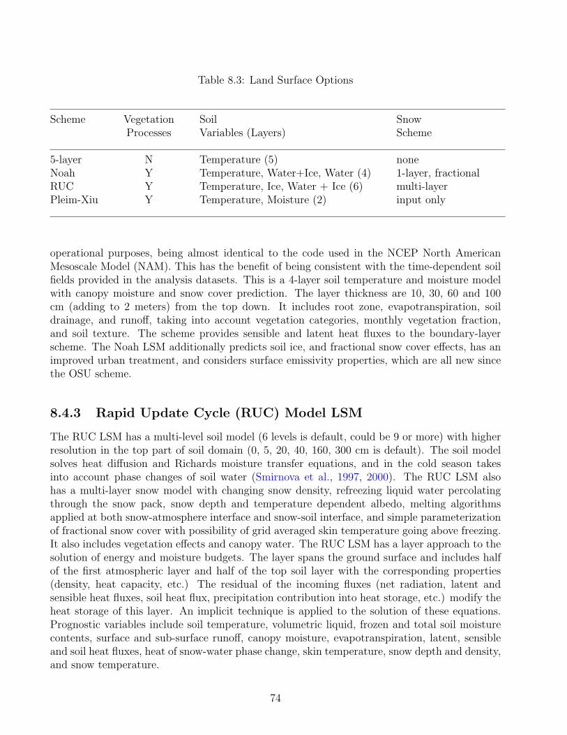
Table 8.3: Land Surface Options

Scheme Vegetation Soil SnowProcesses Variables (Layers) Scheme

5-layer N Temperature (5) noneNoah Y Temperature, Water+Ice, Water (4) 1-layer, fractionalRUC Y Temperature, Ice, Water + Ice (6) multi-layerPleim-Xiu Y Temperature, Moisture (2) input only

operational purposes, being almost identical to the code used in the NCEP North AmericanMesoscale Model (NAM). This has the benefit of being consistent with the time-dependent soilfields provided in the analysis datasets. This is a 4-layer soil temperature and moisture modelwith canopy moisture and snow cover prediction. The layer thickness are 10, 30, 60 and 100cm (adding to 2 meters) from the top down. It includes root zone, evapotranspiration, soildrainage, and runoff, taking into account vegetation categories, monthly vegetation fraction,and soil texture. The scheme provides sensible and latent heat fluxes to the boundary-layerscheme. The Noah LSM additionally predicts soil ice, and fractional snow cover effects, has animproved urban treatment, and considers surface emissivity properties, which are all new sincethe OSU scheme.

8.4.3 Rapid Update Cycle (RUC) Model LSM

The RUC LSM has a multi-level soil model (6 levels is default, could be 9 or more) with higherresolution in the top part of soil domain (0, 5, 20, 40, 160, 300 cm is default). The soil modelsolves heat diffusion and Richards moisture transfer equations, and in the cold season takesinto account phase changes of soil water (Smirnova et al., 1997, 2000). The RUC LSM alsohas a multi-layer snow model with changing snow density, refreezing liquid water percolatingthrough the snow pack, snow depth and temperature dependent albedo, melting algorithmsapplied at both snow-atmosphere interface and snow-soil interface, and simple parameterizationof fractional snow cover with possibility of grid averaged skin temperature going above freezing.It also includes vegetation effects and canopy water. The RUC LSM has a layer approach to thesolution of energy and moisture budgets. The layer spans the ground surface and includes halfof the first atmospheric layer and half of the top soil layer with the corresponding properties(density, heat capacity, etc.) The residual of the incoming fluxes (net radiation, latent andsensible heat fluxes, soil heat flux, precipitation contribution into heat storage, etc.) modify theheat storage of this layer. An implicit technique is applied to the solution of these equations.Prognostic variables include soil temperature, volumetric liquid, frozen and total soil moisturecontents, surface and sub-surface runoff, canopy moisture, evapotranspiration, latent, sensibleand soil heat fluxes, heat of snow-water phase change, skin temperature, snow depth and density,and snow temperature.

74

8.4.4 Pleim-Xiu LSM

The PX LSM (Pleim and Xiu, 1995; Xiu and Pleim, 2001), originally based on the ISBA modelNoilhan and Planton (1989), includes a 2-layer force-restore soil temperature and moisturemodel. The top layer is taken to be 1 cm thick, and the lower layer is 99 cm. The PXLSM features three pathways for moisture fluxes: evapotranspiration, soil evaporation, andevaporation from wet canopies. Evapotranspiration is controlled by bulk stomatal resistance thatis dependent on root zone soil moisture, photosynthetically active radiation, air temperature,and the relative humidity at the leaf surface. Grid aggregate vegetation and soil parametersare derived from fractional coverages of land use categories and soil texture types. There aretwo indirect nudging schemes that correct biases in 2-m air temperature and RH by dynamicadjustment of soil moisture (Pleim and Xiu, 2003) and deep soil temperature (Pleim and Gilliam,2008). Note that a small utility program (ipxwrf) can be used to propagate soil moisture andtemperature between consecutive runs to create a continuous simulation of these quantities.

8.4.5 Urban Canopy Model

This can be run as an option with the Noah LSM. In order to represent the city scale effectson the mesoscale, an urban canopy model (UCM) originally developed by Kusaka et al. (2001)and Kusaka and Kimura (2004) and later on modified by Chen et al. (2006), is coupled to theWRF model via Noah Land surface model. In the UCM, all the urban effects in the vertical areassumed to be subgrid scale meaning that the urban processes are occurring below the lowestmodel level. The urban canopy model includes:

• (i) Parameterization of Street canyons to represent the urban geometry.• (ii) Shadowing from building and radiation reflection.• (iii) An exponential wind profile in the canopy layer• (iv) multilayer heat equation from roof wall and road surfaces.

The urban canopy model estimates the surface temperature and heat fluxes from the roof,wall and road surface. It also calculates the momentum exchange between the urban surfaceand the atmosphere. If they are available, the UCM can take three dfferent densities of urbandevelopment using special land-use categories. In Version 3, an anthropogenic heating diurnalcycle was added as an option.

8.4.6 Ocean Mixed-Layer Model

This can be selected with the 5-layer option, and is designed for hurricane modeling in order tosimulate the cooling of the ocean underneath hurricanes. The ocean mixed-layer model is basedon that of Pollard et al. (1973). Each column is independently coupled to the local atmosphericcolumn, so the model is one-dimensional. The ocean part consists of a time-varying layer,representing the variable-depth mixed layer over a fixed layer acting as a reservoir of coolerwater with a specified thermal lapse rate. In the mixed layer, the prognostic variables are itsdepth, vector horizontal current, and mean temperature taken to be the sea-surface temperature(SST). The hurricane winds drive the current, which in turn leads to mixing at the base of themixed layer when the Richardson number becomes low enough. This mixing deepens and cools

75

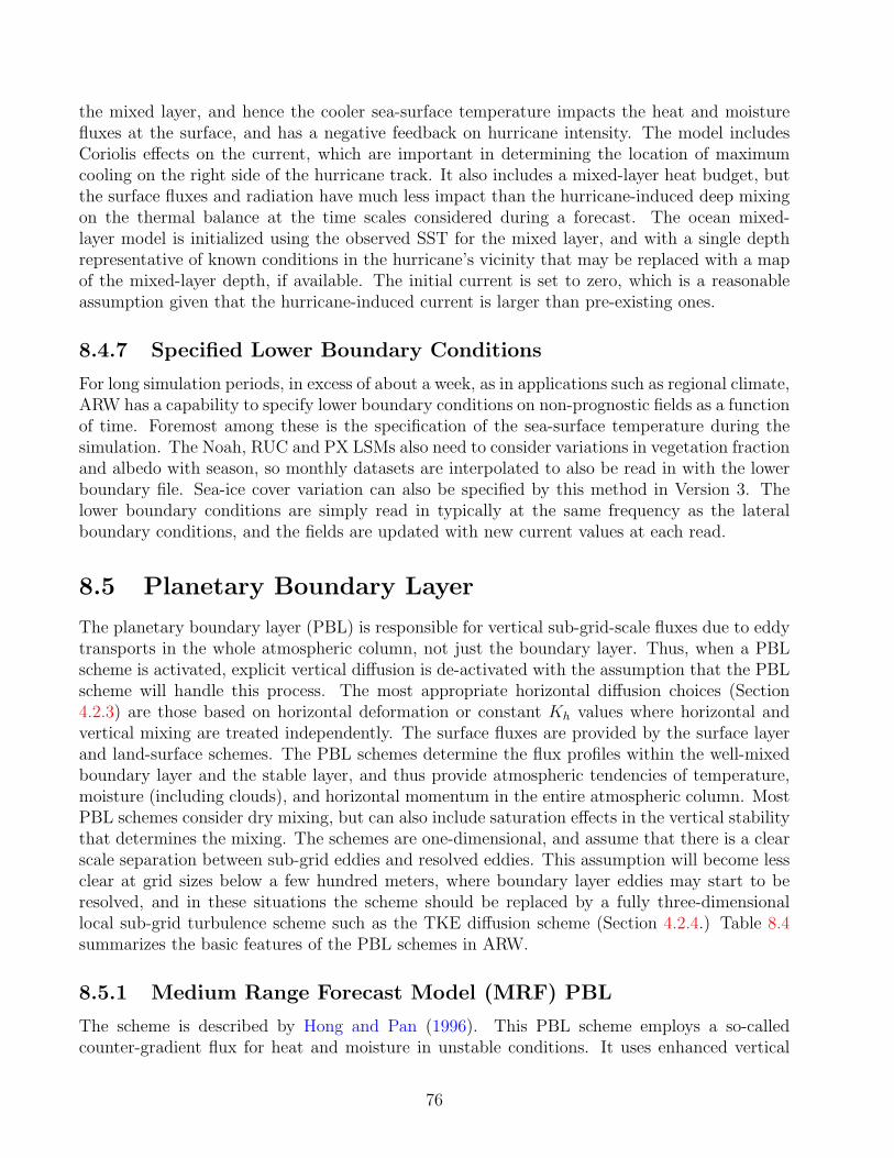
the mixed layer, and hence the cooler sea-surface temperature impacts the heat and moisturefluxes at the surface, and has a negative feedback on hurricane intensity. The model includesCoriolis effects on the current, which are important in determining the location of maximumcooling on the right side of the hurricane track. It also includes a mixed-layer heat budget, butthe surface fluxes and radiation have much less impact than the hurricane-induced deep mixingon the thermal balance at the time scales considered during a forecast. The ocean mixed-layer model is initialized using the observed SST for the mixed layer, and with a single depthrepresentative of known conditions in the hurricane’s vicinity that may be replaced with a mapof the mixed-layer depth, if available. The initial current is set to zero, which is a reasonableassumption given that the hurricane-induced current is larger than pre-existing ones.

8.4.7 Specified Lower Boundary Conditions

For long simulation periods, in excess of about a week, as in applications such as regional climate,ARW has a capability to specify lower boundary conditions on non-prognostic fields as a functionof time. Foremost among these is the specification of the sea-surface temperature during thesimulation. The Noah, RUC and PX LSMs also need to consider variations in vegetation fractionand albedo with season, so monthly datasets are interpolated to also be read in with the lowerboundary file. Sea-ice cover variation can also be specified by this method in Version 3. Thelower boundary conditions are simply read in typically at the same frequency as the lateralboundary conditions, and the fields are updated with new current values at each read.

8.5 Planetary Boundary Layer

The planetary boundary layer (PBL) is responsible for vertical sub-grid-scale fluxes due to eddytransports in the whole atmospheric column, not just the boundary layer. Thus, when a PBLscheme is activated, explicit vertical diffusion is de-activated with the assumption that the PBLscheme will handle this process. The most appropriate horizontal diffusion choices (Section4.2.3) are those based on horizontal deformation or constant Kh values where horizontal andvertical mixing are treated independently. The surface fluxes are provided by the surface layerand land-surface schemes. The PBL schemes determine the flux profiles within the well-mixedboundary layer and the stable layer, and thus provide atmospheric tendencies of temperature,moisture (including clouds), and horizontal momentum in the entire atmospheric column. MostPBL schemes consider dry mixing, but can also include saturation effects in the vertical stabilitythat determines the mixing. The schemes are one-dimensional, and assume that there is a clearscale separation between sub-grid eddies and resolved eddies. This assumption will become lessclear at grid sizes below a few hundred meters, where boundary layer eddies may start to beresolved, and in these situations the scheme should be replaced by a fully three-dimensionallocal sub-grid turbulence scheme such as the TKE diffusion scheme (Section 4.2.4.) Table 8.4summarizes the basic features of the PBL schemes in ARW.

8.5.1 Medium Range Forecast Model (MRF) PBL

The scheme is described by Hong and Pan (1996). This PBL scheme employs a so-calledcounter-gradient flux for heat and moisture in unstable conditions. It uses enhanced vertical

76

Table 8.4: Planetary Boundary Layer Options

Scheme Unstable PBL Entrainment PBL TopMixing treatment

MRF K profile + countergradient term part of PBL mixing from critical bulk Ri

YSU K profile + countergradient term explicit term from buoyancy profileMYJ K from prognostic TKE part of PBL mixing from TKEACM2 transilient mixing up, local K down part of PBL mixing from critical bulk Ri

flux coefficients in the PBL, and the PBL height is determined from a critical bulk Richardsonnumber. It handles vertical diffusion with an implicit local scheme, and it is based on local Ri

in the free atmosphere.

8.5.2 Yonsei University (YSU) PBL

The Yonsei University PBL (Hong et al., 2006) is the next generation of the MRF PBL, alsousing the countergradient terms to represent fluxes due to non-local gradients. This adds tothe MRF PBL (Hong and Pan, 1996) an explicit treatment of the entrainment layer at thePBL top. The entrainment is made proportional to the surface buoyancy flux in line withresults from studies with large-eddy models (Noh et al., 2003). The PBL top is defined usinga critical bulk Richardson number of zero (compared to 0.5 in the MRF PBL), so is effectivelydependent on the buoyancy profile, in which the PBL top is defined at the maximum entrainmentlayer (compared to the layer at which the diffusivity becomes zero). A smaller magnitude ofthe counter-gradient mixing in the YSU PBL produces a well-mixed boundary-layer profile,whereas there is a pronounced over-stable structure in the upper part of the mixed layer in thecase of the MRF PBL. Details are available in Hong et al. (2006), including the analysis of theinteraction between the boundary layer and precipitation physics. In version 3.0, an enhancedstable boundary-layer diffusion algorithm (Hong, 2007) is also devised that allows deeper mixingin windier conditions.

8.5.3 Mellor-Yamada-Janjic (MYJ) PBL

This parameterization of turbulence in the PBL and in the free atmosphere (Janjic, 1990, 1996,2002) represents a nonsingular implementation of the Mellor-Yamada Level 2.5 turbulence clo-sure model (Mellor and Yamada, 1982) through the full range of atmospheric turbulent regimes.In this implementation, an upper limit is imposed on the master length scale. This upper limitdepends on the TKE as well as the buoyancy and shear of the driving flow. In the unstablerange, the functional form of the upper limit is derived from the requirement that the TKE pro-duction be nonsingular in the case of growing turbulence. In the stable range, the upper limitis derived from the requirement that the ratio of the variance of the vertical velocity deviationand TKE cannot be smaller than that corresponding to the regime of vanishing turbulence. The

77

TKE production/dissipation differential equation is solved iteratively. The empirical constantshave been revised as well (Janjic, 1996, 2002).

8.5.4 Asymmetrical Convective Model version 2 (ACM2) PBL

The ACM2 (Pleim, 2007) is a combination of the ACM, which is a simple transilient model thatwas originally a modification of the Blackadar convective model, and an eddy diffusion model.Thus, in convective conditions the ACM2 can simulate rapid upward transport in buoyantplumes and local shear induced turbulent diffusion. The partitioning between the local and non-local transport components is derived from the fraction of non-local heat flux according to themodel of Holtslag and Boville (1993). The algorithm transitions smoothly from eddy diffusionin stable conditions to the combined local and non-local transport in unstable conditions. TheACM2 is particularly well suited for consistent PBL transport of any atmospheric quantityincluding both meteorological (u, v,θ , qv) and chemical trace species.

8.6 Atmospheric Radiation

The radiation schemes provide atmospheric heating due to radiative flux divergence and surfacedownward longwave and shortwave radiation for the ground heat budget. Longwave radiationincludes infrared or thermal radiation absorbed and emitted by gases and surfaces. Upwardlongwave radiative flux from the ground is determined by the surface emissivity that in turndepends upon land-use type, as well as the ground (skin) temperature. Shortwave radiationincludes visible and surrounding wavelengths that make up the solar spectrum. Hence, the onlysource is the Sun, but processes include absorption, reflection, and scattering in the atmosphereand at surfaces. For shortwave radiation, the upward flux is the reflection due to surface albedo.Within the atmosphere the radiation responds to model-predicted cloud and water vapor dis-tributions, as well as specified carbon dioxide, ozone, and (optionally) trace gas concentrations.All the radiation schemes in WRF currently are column (one-dimensional) schemes, so each col-umn is treated independently, and the fluxes correspond to those in infinite horizontally uniformplanes, which is a good approximation if the vertical thickness of the model layers is much lessthan the horizontal grid length. This assumption would become less accurate at high horizontalresolution. Table 8.5 summarizes the basic features of the radiation schemes in the ARW.

8.6.1 Rapid Radiative Transfer Model (RRTM) Longwave

This RRTM, which is taken from MM5, is based on Mlawer et al. (1997) and is a spectral-bandscheme using the correlated-k method. It uses pre-set tables to accurately represent longwaveprocesses due to water vapor, ozone, CO2, and trace gases (if present), as well as accounting forcloud optical depth.

78

Table 8.5: Radiation Options

Scheme Longwave/ Spectral CO2, O3, cloudsShortwave Bands

RRTM LW 16 CO2, O3, cloudsGFDL LW LW 14 CO2, O3, cloudsCAM3 LW LW 2 CO2, O3, cloudsGFDL SW SW 12 CO2, O3, cloudsMM5 SW SW 1 cloudsGoddard SW 11 CO2, O3, cloudsCAM3 SW SW 19 CO2, O3, clouds

8.6.2 Eta Geophysical Fluid Dynamics Laboratory (GFDL) Long-wave

This longwave radiation scheme is from GFDL. It follows the simplified exchange method ofFels and Schwarzkopf (1975) and Schwarzkopf and Fels (1991), with calculation over spectralbands associated with carbon dioxide, water vapor, and ozone. Included are Schwarzkopf andFels (1985) transmission coefficients for carbon dioxide, a Roberts et al. (1976) water vaporcontinuum, and the effects of water vapor-carbon dioxide overlap and of a Voigt line-shapecorrection. The Rodgers (1968) formulation is adopted for ozone absorption. Clouds are ran-domly overlapped. This scheme is implemented to conduct comparisons with the operationalEta model.

8.6.3 CAM Longwave

A spectral-band scheme used in the NCAR Community Atmosphere Model (CAM 3.0) forclimate simulations. It has the potential to handle several trace gases. It interacts with resolvedclouds and cloud fractions, and is documented fully by Collins et al. (2004).

8.6.4 Eta Geophysical Fluid Dynamics Laboratory (GFDL) Short-wave

This shortwave radiation is a GFDL version of the Lacis and Hansen (1974) parameterization.Effects of atmospheric water vapor, ozone (both from Lacis and Hansen, 1974), and carbondioxide (Sasamori et al., 1972) are employed. Clouds are randomly overlapped. Shortwavecalculations are made using a daylight-mean cosine solar zenith angle over the time interval(given by the radiation call frequency).

79

8.6.5 MM5 (Dudhia) Shortwave

This scheme is base on Dudhia (1989) and is taken from MM5. It has a simple downwardintegration of solar flux, accounting for clear-air scattering, water vapor absorption (Lacis andHansen, 1974), and cloud albedo and absorption. It uses look-up tables for clouds from Stephens(1978). In Version 3, the scheme has an option to account for terrain slope and shadowing effectson the surface solar flux.

8.6.6 Goddard Shortwave

This scheme is based on Chou and Suarez (1994). It has a total of 11 spectral bands andconsiders diffuse and direct solar radiation components in a two-stream approach that accountsfor scattered and reflected components. Ozone is considered with several climatological profilesavailable.

8.6.7 CAM Shortwave

A spectral-band scheme used in the NCAR Community Atmosphere Model (CAM 3.0) forclimate simulations. It has the ability to handle optical properties of several aerosol typesand trace gases. It uses cloud fractions and overlap assumptions in unsaturated regions, andhas a monthly zonal ozone climatology. It is documented fully by Collins et al. (2004). TheCAM radiation scheme is especially suited for regional climate simulations by having a ozonedistribution that varies during the simulation according to monthly zonal-mean climatologicaldata.

8.7 Physics Interactions

While the model physics parameterizations are categorized in a modular way, it should benoted that there are many interactions between them via the model state variables (potentialtemperature, moisture, wind, etc.) and their tendencies, and via the surface fluxes. Table 8.6summarizes how the various physics processes interact in the model. In the table, i indicatesthat the state variable or flux is required input for the physics scheme, and o indicates that thetendency or flux is a probable output of the scheme. It can be seen that all the physical schemesinteract in some way with the surface physics (land-surface models, and, potentially, coupledocean models). The surface physics, while not explicitly producing tendencies of atmosphericstate variables, is responsible for updating the land-state variables.

Note also that, as mentioned, the microphysics does not output tendencies, but updates theatmospheric state at the end of the model time-step. However, the rest of the o’s in the upperhalf of the table are representative of the physical tendencies of these variables in the model.

The radiation, cumulus parameterization, and boundary-layer schemes all output tendencies,but the tendencies are not added until later in the solver, so from this perspective the orderof call is not important. Moreover, these physics schemes do not have to be called at thesame frequency as each other or the model time step. When lower frequencies are used, theirtendencies are kept constant between calls. This is typically done for the radiation schemes,which are too expensive to call every time, and for the cumulus schemes, for which it is also not

80

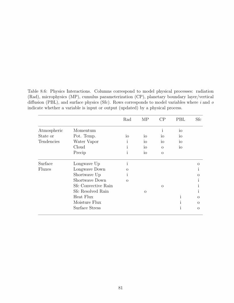
Table 8.6: Physics Interactions. Columns correspond to model physical processes: radiation(Rad), microphysics (MP), cumulus parameterization (CP), planetary boundary layer/verticaldiffusion (PBL), and surface physics (Sfc). Rows corresponds to model variables where i and oindicate whether a variable is input or output (updated) by a physical process.

Rad MP CP PBL Sfc

Atmospheric Momentum i ioState or Pot. Temp. io io io ioTendencies Water Vapor i io io io

Cloud i io o ioPrecip i io o

Surface Longwave Up i oFluxes Longwave Down o i

Shortwave Up i oShortwave Down o iSfc Convective Rain o iSfc Resolved Rain o iHeat Flux i oMoisture Flux i oSurface Stress i o

81

necessary. However, the surface/boundary-layer schemes are normally called every step in theARW because this is likely to give the best results.

The radiation is called first because of the required radiative fluxes that are input to theland-surface scheme. The land-surface also requires rainfall from the microphysics and cumulusschemes, but that is from the previous time-step. The boundary-layer scheme is necessarily afterthe land-surface scheme because it requires the heat and moisture fluxes.

8.8 Four-Dimensional Data Assimilation

Four-dimensional data assimilation (FDDA), also known as nudging, is a method of keepingsimulations close to analyses and/or observations over the course of an integration. There are twotypes of FDDA that can be used separately or in combination. Grid- or analysis-nudging simplyforces the model simulation towards a series of analyses grid-point by grid-point. Observational-or station-nudging locally forces the simulation towards observational data. These methodsprovide a four-dimensional analysis that is somewhat balanced dynamically, and in terms ofcontinuity, while allowing for complex local topographical or convective variations. Such datasetscan cover long periods, and have particular value in driving off-line air quality or atmosphericchemistry models.

8.8.1 Grid Nudging or Analysis Nudging

Grid nudging is a major component of so-called Four-Dimensional Data Assimilation (FDDA).(Other components are surface-analysis nudging to be developed soon, and observational nudg-ing, developed and released in WRF Version 2.2).

The grid-nudging method is specifically three-dimensional analysis nudging, whereby theatmospheric model is nudged towards time- and space-interpolated analyses using a point-by-point relaxation term. Stauffer and Seaman (1990) originally developed the technique for MM5.

The grid-nudging technique has several major uses.a) Four-dimensional datasets. The model is run with grid-nudging for long periods, e.g.

months, to provide a four-dimensional meteorologically self-consistent dataset that also stays ontrack with the driving analyses. In this way, the model is used as an intelligent interpolator ofanalyses between times, and also accounting better for topographic and convective effects. Asmentioned, the primary use for such datasets is in air quality where the wind fields may be usedto drive off-line chemistry models.

b) Boundary conditions. A nested simulation is run with the outer domain nudged towardsanalyses, and the nest running un-nudged. This provides better temporal detail at the nestboundary than driving it directly from linearly interpolated analyses, as it would be if it werethe outer domain. This technique could also be used in forecasting, where an outer domain isnudged towards global forecast fields that are available in advance of the regional forecast.

c) Dynamic initialization. A pre-forecast period (e.g., -6 hours to 0 hours) is run withnudging using analyses at those times that are already available. This is probably better thana cold-start using just the 0 hour analysis because it gives the model a chance to spin up. Inparticular, the model will have six hours to adjust to topography, and produce cloud fields byhour 0, whereas with a cold start there would be a spin-up phase where waves are produced and

82

clouds are developed. This method could also be combined with 3D-Var techniques that mayprovide the hour 0 analysis.

Grid nudging has been added to ARW using the same input analyses as the WPS pre-processing systems can provide. Since it works on multiple domains in a nesting configuration,it requires multiple time-periods of each nudged domain as input analyses. Given these analyses,the real program produces another input file which is read by the model as nudging is performed.This file contains the gridded analysis 3d fields of the times bracketing the current model timeas the forecast proceeds. The four nudged fields are the two horizontal wind components (u andv), temperature, and specific humidity.

The method is implemented through an extra tendency term in the nudged variable’s equa-tions, e.g.

∂θ

∂t= F (θ) + GθWθ(θ0 − θ)

where F (θ) represents the normal tendency terms due to physics, advection, etc., Gθ is a time-scale controlling the nudging strength, and Wθ is an additional weight in time or space to limitthe nudging as described more below, while θ0 is the time- and space-interpolated analysis fieldvalue towards which the nudging relaxes the solution.

Several options are available to control the nudging.a) Nudging end-time and ramping. Nudging can be turned off during the simulation, as

in dynamical initialization. Since turning nudging off suddenly can lead to noise, there is acapability for ramping the nudging down over a period, typically 1-2 hours to reduce the shock.

b) Strength of nudging. The timescale for nudging can be controlled individually for winds,temperature and moisture. Typically the namelist value of 0.0003 s-1 is used, correspondingto a timescale of about 1 hour, but this may be reduced for moisture where there may be lessconfidence in the analysis versus the details in the model.

c) Nudging in the boundary layer. Sometimes, since the analysis does not resolve the diurnalcycle, it is better not to nudge in the boundary layer to let the model PBL evolve properly,particularly the temperature and moisture fields. Each variable can therefore be selectively notnudged in the model boundary layer, the depth of which is given by the PBL physics.

d) Nudging at low levels. Alternatively the nudging can be deactivated for any of the variablesbelow a certain layer throughout the simulation. For example, the lowest ten layers can be freeof the nudging term.

e) Nudging and nesting. Each of these controls is independently set for each domain whennesting, except for the ramping function, which has one switch for all domains.

8.8.2 Observational or Station Nudging

The observation-nudging FDDA capability allows the model to effectively assimilate tempera-ture, wind and moisture observations from all platforms, measured at any location within themodel domains and any time within a given data assimilation periods With the observation-nudging formulation, each observation directly interacts with the model equations and thus thescheme yields dynamically and diabatically initialized analyses to support the applications thatneed regional 4-D full-field weather and/or to start regional NWP with spun-up initial con-ditions. The observation-nudging scheme, which is an enhanced version of the standard MM5

83

observation-nudging scheme, was implemented into WRF-ARW and has been in the model sinceWRF Version 2.2. More details of the methods can be found in Liu et al. (2008). The most sig-nificant modifications to the standard MM5 observation-nudging scheme (Stauffer and Seaman,1994) that are included in the WRF observation-nudging scheme are summarized as follows:

(1) Added capability to incorporate all, conventional and non-conventional, synoptic andasynoptic data resources, including the twice daily radiosondes; hourly surface, ship and buoyobservations, and special observations from GTS/WMO; NOAA/NESDIS satellite winds de-rived from cloud, water vapor and IR imageries; NOAA/FSL ACARS, AMDAR, TAMDARand other aircraft reports; NOAA/FSL NPN (NOAA Profiler Network) and CAP (CorporativeAgencies Profilers) profilers; the 3-hourly cloud-drifting winds and water-vapor-derived windsfrom NOAA/NESDIS; NASA Quikscat sea surface winds; and high-density, high-frequency ob-servations from various mesonets of government agencies and private companies. In particular,special weights are assigned to the application-specific data, such as the SAMS network, specialsoundings and wind profilers located at and operated by the Army test ranges.

(2) Added capability to assimilate multi-level upper-air observations, such as radiosondes,wind profilers and radiometers, in a vertically coherent way, which is in contrast to the algorithmfor single point observations such as aircraft reports and satellite derived winds.

(3) Surface temperature (at 2 m AGL) and winds (at 10 m AGL) observations are firstadjusted to the first model level according to the similarity theory that is built in the modelsurface-layer physics and the surface-layer stability state at the observation time. The adjustedtemperature and wind innovations at the lowest model level are then used to correct the modelthrough the mixing layer, with weights gradually reduced toward the PBL top.

(4) Steep mountains and valleys severely limit the horizontal correlation distances. Forexample, weather variables on the upwind slope are not correlated with those on the downwindslope. To take account this effect, a terrain-dependent nudging weight correction is designed toeliminate the influence of an observation to a model grid point if the two sites are physicallyseparated by a mountain ridge or a deep valley. More details about the scheme and numericaltest results can be found in Xu et al. (2002). Essentially, for a given observation and grid point,a terrain search is done along the line connecting the grid point and the observation site. Ifthere is a terrain blockage or a valley (deeper than a given depth), the nudging weight for theobservation at the given grid point is set to zero. Currently, this algorithm is applied for surfaceobservations assimilation only.

(5) The scheme was adjusted to accomplish data assimilation on multi-scale domains. Twoadjustments among many are noteworthy. The first is an addition of grid-size-dependent hori-zontal nudging weight for each domain and the corresponding inflation with heights. The secondis adding the capability of double-scans, a two-step observation-nudging relaxation. The idea issimilar to the successive corrections: the first scan, with large influence radii and smaller weights,allows observations to correct large scale fields, while the second scan, with smaller influenceradii and large weights, permits the observation to better define the smaller-scale feature.

(6) Observation-nudging allows the observation correction to be propagated into the modelstate in a given time influence window. One technical difficulty with this is that the model stateis not known at the observation time for computing the observation increment, or innovation,during the first half of the time window. In the Stauffer and Seaman (1994) scheme, at eachtime step within the time influence window, the innovation is calculated (or approximated) bydiffering the observation from the model state at the time step. This obviously leads to dragging

84

the future forecasts toward previous (observation) states. To reduce this error, the innovationcalculation is kept the same as before up to the observation time (this is OK since the modelstate is gradually tacking toward the observation state), but the true innovation s kept and usedduring the later half of the time influence window.

(7) An ability for users to set different nudging time-windows and influence radii for different(nested) domains has been added into WRF since the WRF V3.0 release.

85

Chapter 9

Variational Data Assimilation

An introduction to the basic ideas of variational data assimilation and the WRF-Var system isgiven in this chapter, followed by a brief overview of recent major improvements to WRF-Var.This overview supplements the original description of the three-dimensional variational (3D-Var)algorithm found in Barker et al. (2004). One of the most important additions to WRF-Var is anew utility gen be, used to calculate background error covariances for a user’s own application;it is discussed in the latter half of this chapter. The WRF-Var system is evolving rapidly, and afuture technical note will accompany the general release of the 4D-Var component of WRF-Var.That technical note will include an extensive description of the entire WRF-Var system.

9.1 Introduction

The basic goal of any variational data assimilation system is to produce an optimal estimateof the true atmospheric state at analysis time through iterative solution of a prescribed cost-function (Ide et al., 1997):

J(x) = Jb(x) + Jo(x) =1

2(x− xb)TB−1(x− xb) +

1

2(y − yo)T (E + F)−1(y − yo). (9.1)

The variational problem can be summarized as the iterative minimization of (9.1) to find theanalysis state x that minimizes J(x). This solution represents the a posteriori maximum like-lihood (minimum variance) estimate of the true state of the atmosphere given the two sourcesof a priori data: the first guess (or background) xb and observations yo (Lorenc, 1986). Thefit to individual data points is weighted by estimates of their errors: B, E, and F are the back-ground, observation (instrumental), and representivity error covariance matrices, respectively.Representivity error is an estimate of inaccuracies introduced in the observation operator H

used to transform the gridded analysis x to observation space y = H(x) for comparison againstobservations. This error will be resolution dependent and may also include a contribution fromapproximations (e.g., linearizations) in H.

As described in Barker et al. (2004), the particular variational data assimilation algorithmadopted in WRF-Var is a model-space, incremental formulation of the variational problem. Inthis approach, observations, previous forecasts, their errors, and physical laws are combined toproduce analysis increments xa

, which are added to the first guess xb to provide an updatedanalysis.

87

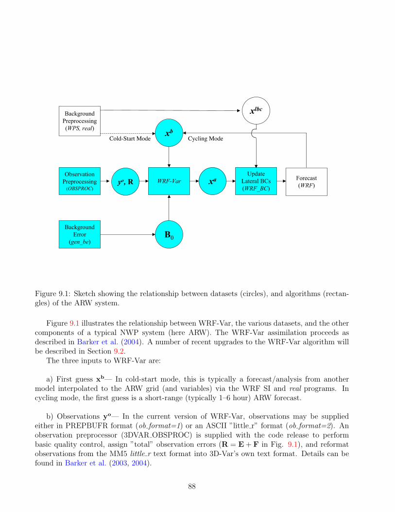
WRF-VarObservation

Preprocessing(OBSPROC)

Background

Error

(gen_be)

Forecast

(WRF)

xb

xayo, R

Update

Lateral BCs

(WRF_BC)

Background

Preprocessing

(WPS, real)

xlbc

Cold-Start Mode

B0

Cycling Mode

Figure 9.1: Sketch showing the relationship between datasets (circles), and algorithms (rectan-gles) of the ARW system.

Figure 9.1 illustrates the relationship between WRF-Var, the various datasets, and the othercomponents of a typical NWP system (here ARW). The WRF-Var assimilation proceeds asdescribed in Barker et al. (2004). A number of recent upgrades to the WRF-Var algorithm willbe described in Section 9.2.

The three inputs to WRF-Var are:

a) First guess xb— In cold-start mode, this is typically a forecast/analysis from anothermodel interpolated to the ARW grid (and variables) via the WRF SI and real programs. Incycling mode, the first guess is a short-range (typically 1–6 hour) ARW forecast.

b) Observations yo— In the current version of WRF-Var, observations may be suppliedeither in PREPBUFR format (ob format=1) or an ASCII ”little r” format (ob format=2). Anobservation preprocessor (3DVAR OBSPROC) is supplied with the code release to performbasic quality control, assign ”total” observation errors (R = E + F in Fig. 9.1), and reformatobservations from the MM5 little r text format into 3D-Var’s own text format. Details can befound in Barker et al. (2003, 2004).

88

c) Background error covariances B— used to define the spatial and multivariate response ofthe analysis to an observation. In variational systems, these covariances are typically calculatedoff-line, and significant tuning is required to optimize performance for a particular application(e.g., Ingleby (2001); Wu et al. (2002)). The amount of work required to do this satisfactorilyis significant, and should not be underestimated. In order to assist the user, WRF developerssupply the following: i) a default set of statistics used for the initial set up of a domain; ii) autility gen be (described in Section 9.3) to process ensembles of forecasts into the appropriatecontrol variable space; and iii) diagnostic routines to assess the accuracy of observation andbackground error statistics. These routines include both innovation vector-based approaches(Hollingsworth and Lonnberg, 1986) and variational tuning approaches (Desroziers and Ivanov,2001).

Following assimilation of all data, an analysis xa is produced that must be merged withthe existing lateral boundary conditions xlbc in the WRF BC utility (Barker et al. (2003)). Atthis stage, the wrfbdy lateral boundary condition files (xlbc) output of WPS/real is updated tomake the lateral boundaries consistent with the analysis, and surface fields (e.g. SST) are alsoupdated in the wrfinput analysis file.

9.2 Improvements to the WRF-Var Algorithm

The latest version of WRF-Var (V3.0) contains a number of improvements relative to that de-scribed in the MM5 3DVAR technical note (Barker et al. (2003)). These are described below.It should also be noted that the public release of WRF-Var V3.0 contains only a subset of thecapabilities of the full WRF-Var system. In particular, the direct assimilation of radiances, hy-brid variational/ensemble data assimilation technique, and 4D-Var will be released once fundingto support these complex algorithms is available.

9.2.1 Improved vertical interpolation

The original WRF 3D-Var system described in Barker et al. (2004) used height interpolationfor all observation operators. If an observation is reported as a function of pressure, then heightis approximated using the hydrostatic relation. This step introduces an unnecessary sourceof error. The new WRF-Var system performs vertical interpolation in terms of the originalobserved coordinate, i.e., pressure or height.

9.2.2 Improved minimization and “outer loop”

Prior to WRF-Var V3.0, the default WRF-Var cost function minimization used a modifiedversion of the limited memory Quasi-Newton Method (QNM). In V3.0, an alternative ConjugateGradient Method (CGM) has been implemented. Unlike the QNM technique, the CGM methodrestricts WRF-Var’s inner loop to be completely linear. This limitation is dealt with throughthe inclusion of an outer loop in WRF-Var, the purpose of which is to iterate towards nonlinearsolutions (e.g., observation operators, balance constraints, and the forecast itself in 4D-Var)using the WRF-Var analysis from the previous iteration as new first guess. The outer loop is alsoused as a form of variational quality control as follows: observations are rejected if the magnitude

89

of the observation minus first guess differences are larger than a specified threshold (typicallyseveral times the observation error standard deviation). This errormax test implicitly assumesthe first guess is accurate. However, in cases when this assumption breaks down (i.e. in areas oflarge forecast error), there is a danger that good observations might be rejected in areas wherethey are most valuable. The outer loop alleviates this effect by allowing observations rejected inprevious iterations to be accepted if their updated observation minus analysis differences passthe errormax QC check in in subsequent outer loops. The assimilation of nearby observationsin previous iterations essentially provides a “buddy check” to the observation in question.

9.2.3 Choice of control variables

A major change that users of previous versions of WRF-Var will notice, is the simplification ofthe background error covariance model used within WRF-Var. As before, the background errorcovariance matrix B is computed not in model space x : u, v, T, q, ps, but in a control variablespace v related to model space via the control variable transform U, i.e.,

x = Uv = UpUvUhv. (9.2)

The expansion U = UpUvUh represents the various stages of covariance modeling: horizontalcorrelations Uh, vertical covariances Uv, and multivariate covariances Up.

The components of v are chosen so that their error cross-correlations are negligible, thuspermitting the matrix B to be block-diagonalized. The major change in WRF-Var V3.0 isto simplify the control variable transform Up to perform a simple statistical regression as de-scribed in subsection (9.3) below. Testing in numerous applications has shown a general im-provement of forecasts scores using this definition of balance, as compared to the dynamicalgeostrophic//cyclostrophic balance constraint defined in Barker et al. (2003).

9.2.4 First Guess at Appropriate Time (FGAT)

A First Guess at Appropriate Time (FGAT) procedure has been implemented in WRF-Var (Leeet al., 2004). The FGAT capability results in a more accurate calculation of innovation vectors(observation minus first guess difference), and hence a better use of observations when their validtime differs from that of the analysis. FGAT is most effective for the analysis of observationsfrom asynoptic, moving platforms (e.g., aircraft and satellite data).

9.2.5 Radar Data Assimilation

A capability to assimilate Doppler radar radial velocity and reflectivity observations is availablein WRF-Var (Xiao et al., 2005, 2007a,b, 2008). In order to calculate the vertical velocity incre-ment as a result of assimilating the vertical velocity component of radial velocity, the Richarsonbalance equation, which combines the continuity equation, adiabatic thermodynamic equationand hydrostatic relation, and its linear and adjoint codes are introduced. For reflectivity as-similation, total water is used as a control variable. This requires a partitioning between watervapor and hydrometeor increments during the minimization procedure. A warm-rain parame-terization is included to assist the calculation of hydrometeors, which includes condensation ofwater vapor into cloud, accretion of cloud by rain, automatic conversion of cloud to rain, and

90

evaporation of rain to water vapor. The observation operators for Doppler radial velocity andreflectivity are included.

9.2.6 Unified Regional/Global 3D-Var Assimilation

There are many benefits to having a single data assimilation system for regional and global ap-plications. The majority of the code is common to both (observation operators, minimization,background error preconditioning, interpolation, etc.). Technically, the main changes requiredto extend the regional application to global are related to the presence of a) the polar singularity,and b) periodic East-West boundary conditions. Of course, there are also scientific questionsconcerning the optimal mix of observations required for global/regional models, and the choiceof control variables and balance constraints. A unified global/regional data assimilation systemshould therefore be flexible to a variety of thinning/quality-control algorithms and also to alter-native formulations of the background error covariance matrix. This flexibility has been a keydesign requirement throughout the WRF-Var project.

The major difference between regional and global options in WRF-Var is in the definitionof horizontal background error covariances. In regional mode, recursive filters (Purser et al.,2003) are used to project observation information away from the observation location. In globalmode, a spectral decomposition is applied. The main benefits of the spectral technique are a)the isotropic and homogeneous covariances that are implied neatly solve the problems associatedwith the pole (the pole is not a special point in spectral space), and b) horizontal correlationsare defined in terms of a single function— the power spectrum (a function of total wavenumber).However, the isotropy of correlation defined in spectral space is also a weakness— anisotropiesneed to be defined in an alternative manner. One solution to this problem is to replace the spec-tral correlations with grid-point correlations (Purser et al., 2003). An alternative technique is tosupplement the isotropic spectral correlations with an anisotropic component derived via gridtransformations, additional control variables or 4D-Var. Research using the latter techniques isunderway using the WRF-Var system.

The WRF-Var code has been adapted to perform assimilation on a global, regular latitude-longitude grid. The major modifications are as follows.

a) Spectral to grid-point transformations (and their adjoints) have been included in 3D-Varto represent the horizontal component (Uh) of the background error covariance model.

b) A new global WRF-Var registry was created to accommodate the output of global forecastmodels (currently only the Korean Meteorological Administration’s (KMA) global model hasbeen tested). The final analysis increments are written in binary format and added back to theglobal first guess to provide the global analysis in the native model format.

c) Changes have been made to allow for periodic boundary conditions in the East–Westdirection.

d) A number of minor changes have been made to treat the polar rows as special points (e.g.,in the grid-point ψ, χ to u, v wind conversion in the Up transform and the observation operatorsfor polar winds).

91

9.3 Background Error Covariances

Forecast (“first guess” or “background”) error covariances are a vital input to variational dataassimilation systems. They influence the analysis fit to observations and also completely definethe analysis response away from observations. The latter impact is particularly importantin data-sparse areas of the globe. Unlike ensemble filter data assimilation techniques (e.g.,the Ensemble Adjustment Kalman Filter, the Ensemble Transform Kalman Filter), 3/4D-Varsystems do not explicitly evolve forecast error covariances in real-time (although both 4D-Varand hybrid variational/ensemble data assimilation techniques currently being developed withinWRF-Var implement flow-dependent covariances implicitly). Instead, climatologic statisticsare usually estimated offline. The “NMC-method”, in which forecast error covariances areapproximated using forecast difference (e.g., T+48 minus T+24) statistics, is a commonly usedapproach (Parrish and Derber, 1992). Experiments at ECMWF (Fisher, 2003) indicate superiorstatistics may be obtained using a cycling analysis/forecast ensemble prediction system basedon perturbed observations/physics.

Recent advances permit the use of flow-dependent forecast error covariances in 3D/4D-Varthrough, for example, grid transformations (Desroziers, 1997), anisotropic recursive filters (Wuet al., 2002; Purser et al., 2003), or observation-space formulations of the variational problem(Daley and Barker, 2001). Flow-dependence may be enhanced in 4D-Var through the use of theforecast model to provide dynamical consistency to the evolving forecast state during 4D-Var’stime window (Rabier et al., 1998). Still, the practical effort required to specify and implementflow-dependent error covariances in 3/4D-Var is significant.

The development of a unified global/regional WRF-Var system, and its widespread use inthe WRF community has necessitated the development of a new, efficient, portable forecastbackground error covariance calculation code. Numerous applications have also indicated thatsuperior results are obtained if one invests effort in calculating domain-specific error covariances,instead of using the the default statistics supplied with the WRF-Var release. In this section,the new gen be code developed by NCAR/MMM to generate forecast error statistics for use withthe WRF-Var system is described.

The background error covariance matrix is defined as

B = T xxT , (9.3)

where the overbar denotes an average over time and/or geographical area. The true backgrounderror is not known in reality, but is assumed to be statistically well-represented by a model stateperturbation x. In the standard NMC-method (Parrish and Derber, 1992), the perturbationx is given by the difference between two forecasts (e.g., 24 hour minus 12 hour) verifyingat the same time. Climatological estimates of background error may then be obtained byaveraging such forecast differences over a period of time (e.g., one month). An alternativestrategy proposed by (Fisher, 2003) makes use of ensemble forecast output, defining the x

vectors as ensemble perturbations (ensemble minus ensemble mean). In either approach, theend result is an ensemble of model perturbation vectors from which estimates of backgrounderror may be derived. The new gen be utility has been designed to work with either forecastdifference, or ensemble-based, perturbations. Using the NMC-method, x = xT2 − xT1 whereT2 and T1 are the forecast difference times (e.g., 48h minus 24h for global, 24h minus 12h for

92

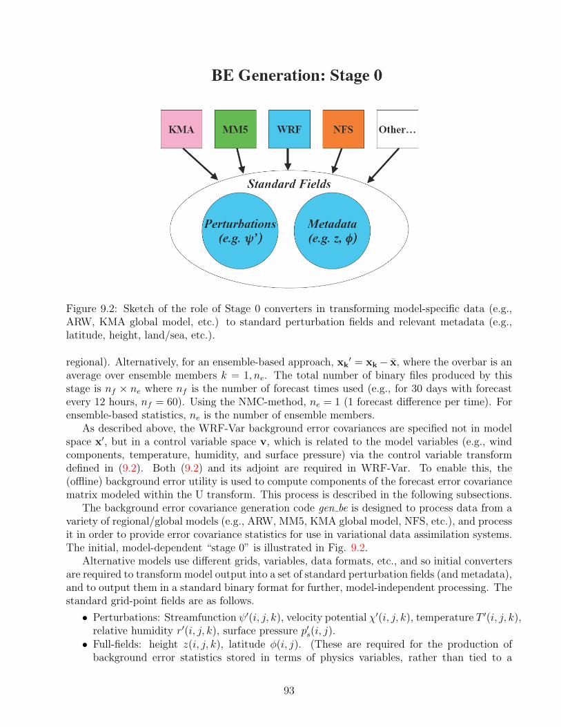
Figure 9.2: Sketch of the role of Stage 0 converters in transforming model-specific data (e.g.,ARW, KMA global model, etc.) to standard perturbation fields and relevant metadata (e.g.,latitude, height, land/sea, etc.).

regional). Alternatively, for an ensemble-based approach, xk = xk− x, where the overbar is an

average over ensemble members k = 1, ne. The total number of binary files produced by thisstage is nf × ne where nf is the number of forecast times used (e.g., for 30 days with forecastevery 12 hours, nf = 60). Using the NMC-method, ne = 1 (1 forecast difference per time). Forensemble-based statistics, ne is the number of ensemble members.

As described above, the WRF-Var background error covariances are specified not in modelspace x, but in a control variable space v, which is related to the model variables (e.g., windcomponents, temperature, humidity, and surface pressure) via the control variable transformdefined in (9.2). Both (9.2) and its adjoint are required in WRF-Var. To enable this, the(offline) background error utility is used to compute components of the forecast error covariancematrix modeled within the U transform. This process is described in the following subsections.

The background error covariance generation code gen be is designed to process data from avariety of regional/global models (e.g., ARW, MM5, KMA global model, NFS, etc.), and processit in order to provide error covariance statistics for use in variational data assimilation systems.The initial, model-dependent “stage 0” is illustrated in Fig. 9.2.

Alternative models use different grids, variables, data formats, etc., and so initial convertersare required to transform model output into a set of standard perturbation fields (and metadata),and to output them in a standard binary format for further, model-independent processing. Thestandard grid-point fields are as follows.

• Perturbations: Streamfunction ψ(i, j, k), velocity potential χ(i, j, k), temperature T

(i, j, k),relative humidity r

(i, j, k), surface pressure ps(i, j).

• Full-fields: height z(i, j, k), latitude φ(i, j). (These are required for the production ofbackground error statistics stored in terms of physics variables, rather than tied to a

93

specific grid. This flexibility is included in gen be through a namelist option to define thebins over which data is averaged in a variety of ways (e.g., latitude height, grid points).Land-sea and orographic effects may also be represented in this way.

In general, the stage 0 converters are developed and maintained by those supporting indi-vidual models. Only the WRF-to-standard-fields converter gen be stage0 wrf is maintained andsupported by the ARW effort.

9.3.1 Removal of time-mean

In order to calculate covariances between fields, the average value must first be removed. Thisis performed in the first stage utility gen be stage1.

9.3.2 Multivariate Covariances: Regression coefficients and unbal-anced variables

The second stage of gen be (gen be stage2) provides statistics for the unbalanced fields χu, Tu,and Psu used as control variables in WRF-Var. The unbalanced control variables are defined asthe difference between full and balanced (or correlated) components of the field. In this stageof the calculation of background errors, the balanced component of particular fields is modeledvia a regression analysis of the field using specified predictor fields (e.g., streamfunction; seeWu et al. (2002) for further details). The resulting regression coefficients are output for usein WRF-Var’s Up transform. Currently, three regression analyses are performed resulting inthree sets of regression coefficients (note: The perturbation notation has been dropped for theremainder of this chapter for clarity.):

• Velocity potential/streamfunction regression: χb(k) = c(k)ψ(k);

• Temperature/streamfunction regression: Tb(k) =

k1 G(k1, k)ψ(k1); and

• Surface pressure/streamfunction regression: psb =

k1 W (k1)ψ(k1).

The summation over the vertical index k1 relates to the integral (hydrostatic) relationshipbetween mass fields and the wind field. By default, the regression coefficients c, G, and W donot vary horizontally, however options exists to relax this assumption via the bin type namelistvariable in order to allow representation of differences between, for example, polar, mid-latitude,and tropical dynamical and physical processes. The scalar coefficient c used to estimate velocitypotential errors from those of streamfunction is permitted to vary with model level in orderto represent, for example, the impact of boundary-layer physics. Latitudinal/height smoothingof the resulting coefficients may be optionally performed to avoid artificial discontinuities atthe edges of latitude/height boxes (see the future WRF-Var technical note for details of these”expert” features).

Having computed regression coefficients, the unbalanced components of the fields are cal-culated as χu(k) = χ(k) − c(k)ψ(k), Tu(k) = T (k) −

k1 G(k1, k)ψ(k1), and psu = ps −

k1 W (k1)ψ(k1). These fields are output for the subsequent calculation of the spatial covari-ances as described below.

94

9.3.3 Vertical Covariances: Eigenvectors/eigenvalues and control vari-able projections

The third stage (gen be stage3) of gen be calculates the statistics required for the vertical com-ponent of the control variable transform. This calculation involves the projection of 3D fieldson model-levels onto empirical orthogonal functions (EOFs) of the vertical component of back-ground error covariances Barker et al. (2004). For each 3D control variable (ψ, χu, Tu, and r),the vertical component of B, is calculated and an eigenvector decomposition performed. Theresulting eigenvectors E and eigenvalues Λ are saved for use in WRF-Var.

The gen be code calculates both domain-averaged and local values of the vertical componentof the background error covariance matrix. Eigendecomposition of the resulting K ×K (K isthe number of vertical levels) climatological vertical error covariance matrix B = EΛET resultsin both domain-averaged and local eigenvectors E and eigenvalues Λ. Both sets of statisticsare included in the dataset supplied to WRF-Var, allowing the choice between homogeneous(domain-averaged) or local (inhomogeneous) background error variances and vertical correlationsto be chosen at run time Barker et al. (2004). Having calculated and stored eigenvectors andeigenvalues, the final part of gen be stage3 is to project the entire sequence of 3D control variablefields into EOF space vv = U

−1v vp = Λ−1/2ETvp.

9.3.4 Horizontal Covariances: Recursive filter lengthscale (regional),or power spectra (global)

The last aspect of the climatological component of background error covariance data required forWRF-Var is the horizontal error correlations, the representation of which forms the largest dif-ference between running WRF-Var in regional and global mode - the rest of gen be is essentiallythe same for both regional and global models.

In a global application (gen be stage4 global), power spectra are computed for each of the K

vertical modes of the 3D control variables ψ, χu, Tu, and relative humidity r, and for the 2Dcontrol variable psu data. In contrast, in regional mode, horizontal correlations are computedbetween grid-points of each 2D field, binned as a function of distance. A Gaussian curve is thenfitted to the data as described in Barker et al. (2004) to provide correlation lengthscales for usein the recursive filter algorithm.

9.4 WRF-Var V3.0 Software Engineering Improvements

A major overhall of the WRF-Var software has been performed for V3.0. The following is asummary:

9.4.1 Memory improvements

The WRF-Var registry had become bloated with WRF and U4D-Var 2d and 3d state variablesthat were unused in 3D-Var applications. These variables were allocated but uninitialised, andwritten to the analysis files. The removal of these dummy variable has resulted in a significant(10-50% depending on application) reduction in the memory requirements of WRF-Var.

95

9.4.2 Four-Byte I/O

The WRF-Var algorithm requires eight-byte precision internally. However, it only needs toread and write 4-byte files. Switching from 8-byte to 4-byte output in V3.0 has improved I/Operformance and halves file sizes.

9.4.3 Switch from RSL to RSL LITE

The switch from RSL to RSL LITE has been made in V3.0 as the latter possesses a simpler”lighter” communications layer, and has been shown to be scalable to arbitrary domain sizes(largest to date: 4500x4500) and numbers of processors (largest to date: 64K processors on BlueGene). RSL LITE supports all capabilities of WRF, including Halo and periodic boundaryexchanges, Distributed I/O, Nesting and moving nests, and parallel transposes. RSL LITEhas also been simplified by dropping irregular decomposition, load balancing, and ragged edgenesting, and the initialisation techniques improved to avoid recalculation and give better scalingat higher processor counts.

9.4.4 Reorganisation of observation structures

The F90 derived data types used for observations have been rewritten to permit batches ofobservations to be passed to subroutine calls, especially interpolation ones and subsequentlymakes better use of cache memory.

9.4.5 Radar reflectivity operators redesigned

The efficiency of the coding of the radar observation operators has been improved. Previously,routines were called once per observation, which would then recalculate common factors beforeperforming what was often just a one-line calculation. Re-writing the code in V3.0 to move thecalculations inside loops in the calling routine allows them to work on batches of observationsat a time, vastly improving cache hit rates and eliminating recalculation.

96

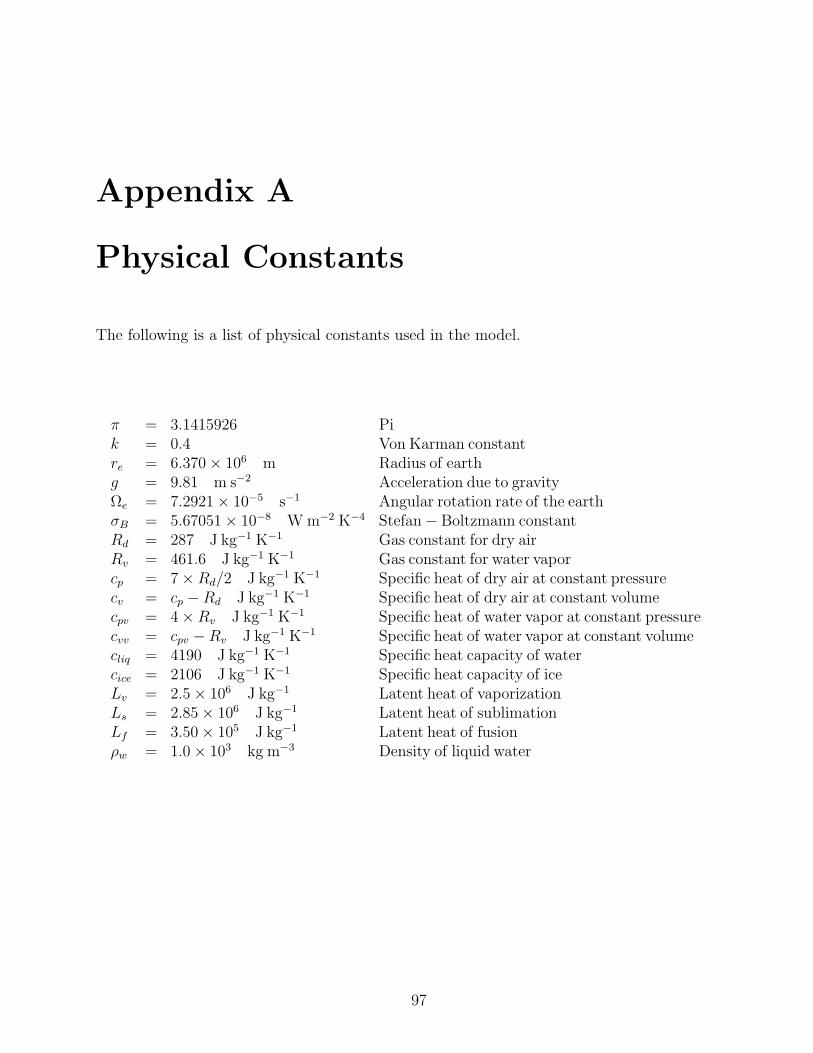
Appendix A

Physical Constants

The following is a list of physical constants used in the model.

π = 3.1415926 Pik = 0.4 Von Karman constantre = 6.370× 106 m Radius of earthg = 9.81 m s−2 Acceleration due to gravityΩe = 7.2921× 10−5 s−1 Angular rotation rate of the earthσB = 5.67051× 10−8 W m−2 K−4 Stefan− Boltzmann constantRd = 287 J kg−1 K−1 Gas constant for dry airRv = 461.6 J kg−1 K−1 Gas constant for water vaporcp = 7×Rd/2 J kg−1 K−1 Specific heat of dry air at constant pressurecv = cp −Rd J kg−1 K−1 Specific heat of dry air at constant volumecpv = 4×Rv J kg−1 K−1 Specific heat of water vapor at constant pressurecvv = cpv −Rv J kg−1 K−1 Specific heat of water vapor at constant volumecliq = 4190 J kg−1 K−1 Specific heat capacity of watercice = 2106 J kg−1 K−1 Specific heat capacity of iceLv = 2.5× 106 J kg−1 Latent heat of vaporizationLs = 2.85× 106 J kg−1 Latent heat of sublimationLf = 3.50× 105 J kg−1 Latent heat of fusionρw = 1.0× 103 kg m−3 Density of liquid water

97

Appendix B

List of Symbols

Symbols used in this document are listed in alphabatical order in this appendix.

Symbols Definition

a generic variableA coefficient (Chapter 4), base-state lapse rate constant (Chapter 5)B background error covariance matrixc scalar coefficientcs speed of soundCk a constant used in TKE closureCr Courant numberCrmax maximum Courant numberCrtheory Courant number from Table 3.1Crβ activation Courant number in vertical velocity dampingCs a constant used in eddy viscosity calculationD deformationDnm deformation tensor, where n,m = 1, 2 and 3e cosine component of the Coriolis term (Chapters 2, 3); turbulent kinetic energy

(Chapter 4)E observation error covariance matrixf sine component of the Coriolis termF forcing terms for U , V , W , Θ and Qm

F representivity error covariance matrixFXcor Coriolis forcing terms for X = U , V , and W

F1,2 coefficients for weighting functions in specified boundary conditiong acceleration due to gravityGk regression coefficientH observation operatorJ cost functionKdh,dv horizontal and vertical eddy viscosity for gravity wave absorbing layerKh,v horizontal and vertical eddy viscosities

99

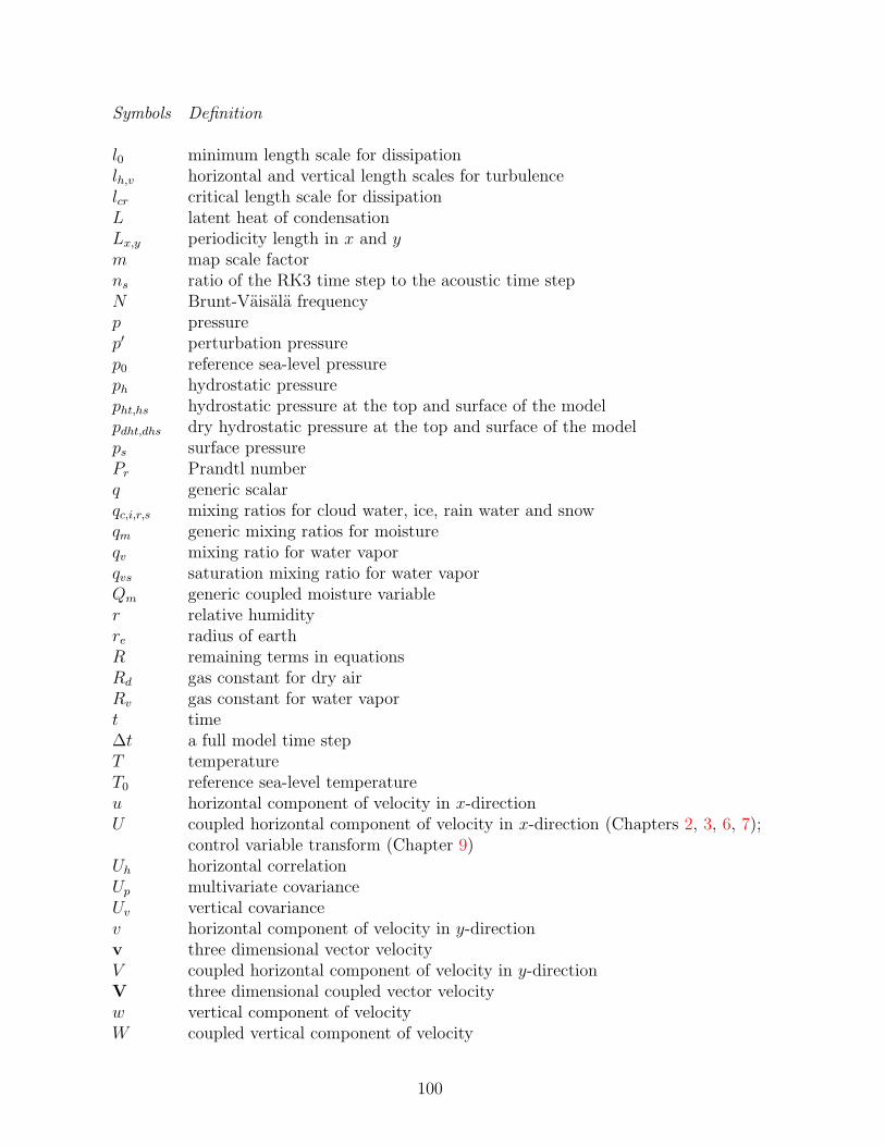
Symbols Definition

l0 minimum length scale for dissipationlh,v horizontal and vertical length scales for turbulencelcr critical length scale for dissipationL latent heat of condensationLx,y periodicity length in x and y

m map scale factorns ratio of the RK3 time step to the acoustic time stepN Brunt-Vaisala frequencyp pressurep perturbation pressure

p0 reference sea-level pressureph hydrostatic pressurepht,hs hydrostatic pressure at the top and surface of the modelpdht,dhs dry hydrostatic pressure at the top and surface of the modelps surface pressurePr Prandtl numberq generic scalarqc,i,r,s mixing ratios for cloud water, ice, rain water and snowqm generic mixing ratios for moistureqv mixing ratio for water vaporqvs saturation mixing ratio for water vaporQm generic coupled moisture variabler relative humidityre radius of earthR remaining terms in equationsRd gas constant for dry airRv gas constant for water vaport time∆t a full model time stepT temperatureT0 reference sea-level temperatureu horizontal component of velocity in x-directionU coupled horizontal component of velocity in x-direction (Chapters 2, 3, 6, 7);

control variable transform (Chapter 9)Uh horizontal correlationUp multivariate covarianceUv vertical covariancev horizontal component of velocity in y-directionv three dimensional vector velocityV coupled horizontal component of velocity in y-directionV three dimensional coupled vector velocityw vertical component of velocityW coupled vertical component of velocity

100

Symbols Definition

Wk regression coefficientz heightzd depth of damping layerztop height of model topα inverse density of airα perturbation inverse density of air

α inverse density of air for the reference stateαd inverse density of dry airαr local rotation angle between y-axis and the meridianβ off-centering coefficient for semi-implicit acoustic stepγ ratio of heat capacities for dry air at constant pressure and volumeγd divergence damping coefficientγe external mode damping coefficientγg damping coefficient for upper boundary gravity wave absorbing layerγr Rayleigh damping coefficient molecular weight of water over the molecular weight of dry air (Chapter 4);

true background error (Chapter 9)η terrain-following hydrostatic-pressure vertical coordinateη contravariant ‘vertical’ velocity or coordinate velocityθ potential temperatureθe equivalent potential temperatureθm moist potential temperatureΘ coupled potential temperatureµ hydrostatic pressure difference between surface and top of the modelµ reference state hydrostatic pressure difference between surface and top of the

modelµd dry hydrostatic pressure difference between surface and top of the modelτ acoustic time (Chapter 3), vertical structure function for Rayleigh damping

(Chapter 4)τnm stress tensor (Chapter 4) where n.m = 1, 2 and 3∆τ acoustic time stepφ geopotential (Chapters 2, 3, 5); latitude (Chapter 9)φ geopotential for reference stateφ perturbation geopotential

Φ generic prognostic variable (coupled)ψ generic variable (Chapter 6)ψ streamfunction increment

χ velocity potential increment

ω same as η

Ω coupled coordinate velocityΩe angular rotation rate of the earth

101

Subscripts/Superscripts Definition

()d dry()h hydrostatic()0 base state sea-level constant() reference state() perturbation from reference state()t∗ full value at a Runge-Kutta step() perturbation from Runge-Kutta step value in acoustic steps

102

Appendix C

Acronyms

AFWA Air Force Weather AgencyAPI Application Program InterfaceARPS Advanced Regional Prediction SystemARW Advanced Research WRFBUFR Binary Universal Form for the Representation of Meteorological DataCAPE Convectively Available Potential EnergyCAPS Center for the Analysis and Prediction of StormsCGM Conjugate Gradient MethodCOAMPS Coupled Ocean / Atmosphere Mesoscale Prediction SystemCOMET Cooperative Program for Operational Meteorology, Education, and TrainingDFI Digital Filtering InitializationDTC Developmental Testbed CenterECMWF The European Centre for Medium-Range Weather ForecastsEOF Empirical Orthogonal FunctionESMF Earth System Modeling FrameworkFAA Federal Aviation AdministrationFGAT First Guess at Appropriate TimeFSL Forecast System LaboratoryGFDL Geophysical Fluid Dynamics LaboratoryGFS Global Forecast SystemGRIB Gridded BinaryKMA Korean Meteorological AdministrationLSM Land Surface ModelMKS Meter Kilogram SecondMM5 Pennsylvania State / NCAR Mesoscale Model Version 5MMM Mesoscale and Microscale Meteorology DivisionMRF Medium Range Forecast ModelNAM North American Mesoscale ModelNCAR National Center for Atmospheric ResearchNCEP National Centers for Environmental PredictionNFS Non-hydrostatic Forecast System (Central Weather Bureau of Taiwan)NMM Nonhydrostatic Mesoscale ModelNOAA National Oceanographic and Atmospheric Administration

103

NRL Navy Research LaboratoryNWP Numerical Weather PredictionOSU Oregon State UniversityPBL Planetary Boundary LayerPPM Piecewise Parabolic MethodQNM Quasi Newton MethodRHS Right Hand SideRRTM Rapid Radiative Transfer ModelRUC Rapid Update CycleSI (WRF) Standard InitializationTKE Turbulent Kinetic EnergyUCAR University Corporation for Atmospheric ResearchYSU Yonsei University (Korea)VAR Variational AssimilationWRF Weather Research and Forecasting ModelWSF WRF Software Framework

104

Bibliography

Barker, D. M., W. Huang, Y.-R. Guo, and A. Bourgeois, 2003: A Three-Dimensional Variational(3DVAR) Data Assimilation System For Use With MM5. NCAR Tech Note, NCAR/TN-453+STR, 68 pp. [Available from UCAR Communications, P.O. Box 3000, Boulder, CO,80307.].

Barker, D. M., W. Huang, Y.-R. Guo, A. Bourgeois, and X. N. Xiao, 2004: A Three-DimensionalVariational Data Assimilation System for MM5: Implementation and Initial Results Mon.Wea. Rev., 132, 897–914.

Beljaars, A.C.M., 1994: The parameterization of surface fluxes in large-scale models under freeconvection, Quart. J. Roy. Meteor. Soc., 121, 255–270.

Betts, A. K., 1986: A new convective adjustment scheme. Part I: Observational and theoreticalbasis. Quart. J. Roy. Meteor. Soc., 112, 677–691.

Betts, A. K., and M. J. Miller, 1986: A new convective adjustment scheme. Part II: Single columntests using GATE wave, BOMEX, and arctic air-mass data sets. Quart. J. Roy. Meteor. Soc.,112, 693–709.

Carpenter, R. L., K. K. Droegemeier, P. R. Woodward, and C. E. Hane, 1990: Application ofthe Piecewise Parabolic Method (PPM) to meteorological modeling. Mon. Wea. Rev., 118,586–612.

Chen, F., and J. Dudhia, 2001: Coupling an advanced land-surface/ hydrology model with thePenn State/ NCAR MM5 modeling system. Part I: Model description and implementation.Mon. Wea. Rev., 129, 569–585.

Chen, F., M. Tewari, H. Kusaka, and T. T. Warner, 2006: Current status of urban modeling inthe community Weather Research and Forecast (WRF) model. Joint with Sixth Symposiumon the Urban Environment and AMS Forum: Managing our Physical and Natural Resources:Successes and Challenges, Atlanta, GA, USA, Amer. Meteor. Soc., CD-ROM. J1.4.

Chen, S.-H., and W.-Y. Sun, 2002: A one-dimensional time dependent cloud model. J. Meteor.Soc. Japan, 80, 99–118.

Chou M.-D., and M. J. Suarez, 1994: An efficient thermal infrared radiation parameterizationfor use in general circulation models. NASA Tech. Memo. 104606, 3, 85pp.

Collins, W.D. et al., 2004: Description of the NCAR Community Atmosphere Model (CAM3.0), NCAR Technical Note, NCAR/TN-464+STR, 226pp.

105

Cooper, W. A., 1986: Ice initiation in natural clouds. Precipitation Enhancement — A ScientificChallenge, Meteor. Monogr., No. 43, Amer. Met. Soc., 29–32.

Daley, R., and E. Barker, 2001: NAVDAS: Formulation and Diagnostics. Mon. Wea. Rev., 129,869–883.

Davies, H. C., and R. E. Turner, 1977: Updating prediction models by dynamical relaxation:An examination of the technique. Quart. J. Roy. Meteor. Soc., 103, 225–245.

Deardorff, J. W., 1972 Numerical investigation of neutral and unstable planetary boundarylayers, J. Atmos. Sci., 29, 91–115.

Desroziers, G., 1997: A coordinate change for data assimilation in spherical geometry of frontalstructures. Mon. Wea. Rev., 125, 3030–3039.

Desroziers, G., and S. Ivanov, 2001: Diagnosis and adaptive tuning of observation-error param-eters in a variational assimilation. Quart. J. Roy. Meteor. Soc., 127, 1433–1452.

Dudhia, J., 1989: Numerical study of convection observed during the winter monsoon experimentusing a mesoscale two-dimensional model, J. Atmos. Sci., 46, 3077–3107.

Dudhia, J., 1995: Reply, Mon. Wea. Rev., 123, 2571–2575.

Dudhia, J., S.-Y. Hong, and K.-S. Lim, 2008: A new method for representing mixed-phaseparticle fall speeds in bulk microphysics parameterizations. J. Met. Soc. Japan, in press.

Durran, R. D., and J. B. Klemp, 1983: A compressible model for the simulation of moistmountain waves, Mon. Wea. Rev., 111, 2341–2361.

Dyer, A. J., and B. B. Hicks, 1970: Flux-gradient relationships in the constant flux layer, Quart.J. Roy. Meteor. Soc., 96, 715–721.

Easter, R. C., 1993: Two modified versions of Bott’s positive definite numerical advectionscheme. Mon. Wea. Rev., 121, 297–304.

Fels, S. B. and M. D. Schwarzkopf, 1975: The Simplified Exchange Approximation: A NewMethod for Radiative Transfer Calculations, J. Atmos. Sci., 32, 1475–1488.

Fisher, M., 2003: Background error covariance modeling. Seminar on Recent Development inData Assimilation for Atmosphere and Ocean, 45–63, ECMWF.

Fletcher, N. H., 1962: The Physics Of Rain Clouds. Cambridge University Press, 386 pp.

Grell, G. A., and D. Devenyi, 2002: A generalized approach to parameterizing convection com-bining ensemble and data assimilation techniques. Geophys. Res. Lett., 29(14), Article 1693.

Grell, G.A., S.E. Peckham, R. Schmitz, S.A. McKeen, G. Frost, W.C. Skamarock and B. Eder,2005: Fully coupled online chemistry within the WRF model. Atmos. Environ., 39, 6957-6975.

Haltiner, G. J., and R. T. Williams, 1980: Numerical prediction and dynamic meteorology. JohnWiley & Sons, Inc., 477pp.

106

Hollingsworth, A., and P. Lonnberg, 1986: The Statistical Structure Of Short-Range ForecastErrors As Determined From Radiosonde Data. Part I: The Wind Field. Tellus, 38A, 111–136.

Holtslag, A. A. M. and B. A. Boville, 1993: Local versus non-local boundary layer diffusion ina global climate model, J. Climate, 6, 1825–1842.

Hong, S.-Y., 2007: Stable Boundary Layer Mixing in a Vertical Diffusion Scheme. The KoreaMeteor. Soc., Fall conference, Seoul, Korea, Oct. 25-26.

Hong, S.-Y., and J.-O. J. Lim, 2006: The WRF Single-Moment 6-Class Microphysics Scheme(WSM6), J. Korean Meteor. Soc., 42, 129–151.

Hong, S.-Y., and H.-L. Pan, 1996: Nonlocal boundary layer vertical diffusion in a medium-rangeforecast model, Mon. Wea. Rev., 124, 2322–2339.

Hong, S.-Y., H.-M. H. Juang, and Q. Zhao, 1998: Implementation of prognostic cloud schemefor a regional spectral model, Mon. Wea. Rev., 126, 2621–2639.

Hong, S.-Y., J. Dudhia, and S.-H. Chen, 2004: A Revised Approach to Ice Microphysical Pro-cesses for the Bulk Parameterization of Clouds and Precipitation, Mon. Wea. Rev., 132,103–120.

Hong, S.-Y., and Y. Noh, and J. Dudhia, 2006: A new vertical diffusion package with an explicittreatment of entrainment processes. Mon. Wea. Rev., 134, 2318–2341.

Huang, X.-Y. and P. Lynch, 1993: Diabatic Digital-Filtering Initialization: Application to theHIRLAM Model., Mon. Wea. Rev., 121, 589–603.

Ide, K., P. Courtier, M. Ghil, and A. C. Lorenc, 1997: Unified notation for data assimilation:Operational, sequential and variational. J. Met. Soc. Japan, 75, 181–189.

Ingleby, N. B., 2001: The statistical structure of forecast errors and its representation in theMet. Office global 3-D variational data assimilation scheme. Quart. J. Roy. Meteor. Soc., 127,209–232.

Janjic, Z. I., 1990: The step-mountain coordinate: physical package, Mon. Wea. Rev., 118,1429–1443.

Janjic, Z. I., 1994: The step-mountain eta coordinate model: further developments of the con-vection, viscous sublayer and turbulence closure schemes, Mon. Wea. Rev., 122, 927–945.

Janjic, Z. I., 1996: The surface layer in the NCEP Eta Model, Eleventh Conference on NumericalWeather Prediction, Norfolk, VA, 19–23 August; Amer. Meteor. Soc., Boston, MA, 354–355.

Janjic, Z. I., 2000: Comments on ”Development and Evaluation of a Convection Scheme for Usein Climate Models”, J. Atmos. Sci., 57, p. 3686.

Janjic, Z. I., 2002: Nonsingular Implementation of the Mellor–Yamada Level 2.5 Scheme in theNCEP Meso model, NCEP Office Note, No. 437, 61 pp.

107

Kain, J. S., and J. M. Fritsch, 1990: A one-dimensional entraining/ detraining plume modeland its application in convective parameterization, J. Atmos. Sci., 47, 2784–2802.

Kain, J. S., and J. M. Fritsch, 1993: Convective parameterization for mesoscale models: TheKain-Fritcsh scheme, The representation of cumulus convection in numerical models, K. A.Emanuel and D.J. Raymond, Eds., Amer. Meteor. Soc., 246 pp.

Kain, J. S., 2004: The Kain-Fritsch convective parameterization: An update. J. Appl. Meteor.,43, 170–181.

Kessler, E., 1969: On the distribution and continuity of water substance in atmospheric circu-lation, Meteor. Monogr., 32, Amer. Meteor. Soc., 84 pp.

Klemp, J. B., and D. K. Lilly, 1978: Numerical simulation of hydrostatic mountain waves, J.Atmos. Sci., 35, 78–107.

Klemp, J. B., and R. Wilhelmson, 1978: The simulation of three-dimensional convective stormdynamics, J. Atmos. Sci., 35, 1070–1096.

Klemp, J. B., W. C. Skamarock, and J. Dudhia, 2007: Conservative split-explicit time in-tegration methods for the compressible nonhydrostatic equations, Mon. Wea. Rev.., 135,2897–2913.

Klemp, J. B., J. Dudhia, and A. Hassiotis, 2008: An Upper Gravity Wave Absorbing Layer forNWP Applications. Mon. Wea. Rev.., submitted.

Knievel, J. C., G. H. Bryan, and J. P. Hacker, 2007: Explicit numerical diffusion in the WRFModel. Mon. Wea. Rev., 135, 3808–3824.

Kusaka, H. and F. Kimura, 2004: Coupling a single-layer urban canopy model with a simpleatmospheric model: Impact on urban heat island simulation for an idealized case. J. Meteor.Soc. Japan, 82, 67–80.

Kusaka, H., H. Kondo, Y. Kikegawa, and F. Kimura, 2001: A simple single-layer urban canopymodel for atmospheric models: Comparison with multi-layer and slab models. Bound.-LayerMeteor., 101, 329–358.

Lacis, A. A., and J. E. Hansen, 1974: A parameterization for the absorption of solar radiationin the earth’s atmosphere. J. Atmos. Sci., 31, 118–133.

Laprise R., 1992: The Euler Equations of motion with hydrostatic pressure as as independentvariable, Mon. Wea. Rev., 120, 197–207.

Lee, M.-S., D. Barker, W. Huang and Y.-H. Kuo, 2004: First Guess at Appropriate Time(FGAT) with WRF 3DVAR. WRF/MM5 Users Workshop, 22–25 June 2004, Boulder, Col-orado.

Lin, Y.-L., R. D. Farley, and H. D. Orville, 1983: Bulk parameterization of the snow field in acloud model. J. Climate Appl. Meteor., 22, 1065–1092.

108

Lin, S.-J., and R. B. Rood, 1996: Multidimensional flux-form semi-Lagrangian transportschemes. Mon. Wea. Rev., 124, 2046–2070.

Liu, Y., T.T. Warner, J. F. Bowers, L. P. Carson, F. Chen, C. A. Clough, C. A. Davis, C. H.Egeland, S. Halvorson, T.W. Huck Jr., L. Lachapelle, R.E. Malone, D. L. Rife, R.-S. Sheu,S. P. Swerdlin, and D.S. Weingarten, 2008: The operational mesogamma-scale analysis andforecast system of the U.S. Army Test and Evaluation Command. Part 1: Overview of themodeling system, the forecast products. J. Appl. Meteor. Clim., 47, 1077–1092.

Lorenc, A. C., 1986: Analysis methods for numerical weather prediction. Quart. J. Roy. Meteor.Soc., 112, 1177–1194.

Lynch, P., and X.-Y. Huang, 1992: Initialization of the HIRLAM Model Using a Digital Filter.Mon. Wea. Rev., 120, 1019–1034.

Lynch, P., and X.-Y. Huang, 1994: Diabatic initialization using recursive filters. Tellus, 46A,583–597.

Lynch, P., 1997: The Dolph-Chebyshev Window: A Simple Optimal Filter. Mon. Wea. Rev.,125, 655–660.

McCumber, M., W.-K. Tao, J. Simpson, R. Penc, and S.-T. Soong, 1991: Comparison of ice-phase microphysical parameterization schemes using numerical simulations of tropical con-vection, J. Appl. Meteor., 30, 985–1004.

Mellor, G. L., and T. Yamada, 1982: Development of a turbulence closure model for geophysicalfluid problems. Rev. Geophys. Space Phys., 20, 851–875.

Michalakes, J., J. Dudhia, D. Gill, J. Klemp, and W. Skamarock, 1999: Design of a next-generation regional weather research and forecast model, Towards Teracomputing, World Sci-entific, River Edge, New Jersey, 117–124.

Michalakes, J., J. Dudhia, D. Gill, T. Henderson, J. Klemp, W. Skamarock, and W. Wang,2004: The Weather Research and Forecast Model: Software Architecture and Performance.To appear in proceeding of the Eleventh ECMWF Workshop on the Use of High PerformanceComputing in Meteorology. 25–29 October 2004, Reading, U.K., Ed. George Mozdzynski.

Mlawer, E. J., S. J. Taubman, P. D. Brown, M. J. Iacono, and S. A. Clough, 1997: Radiativetransfer for inhomogeneous atmosphere: RRTM, a validated correlated-k model for the long-wave. J. Geophys. Res., 102 (D14), 16663–16682.

Monin, A.S. and A.M. Obukhov, 1954: Basic laws of turbulent mixing in the surface layer ofthe atmosphere. Contrib. Geophys. Inst. Acad. Sci., USSR, (151), 163–187 (in Russian).

Morrison, H., J. A. Curry, and V. I. Khvorostyanov, 2005: A new double-moment microphysicsparameterization for application in cloud and climate models, Part I: Description. J. Atmos.Sci., 62, 1665–1677.

109

Morrison, H., and J. O. Pinto, 2006: Intercomparison of bulk microphysics schemes in mesoscalesimulations of springtime Arctic mixed-phase stratiform clouds. Mon. Wea. Rev., 134, 1880–1900.

Morrison, H., G. Thompson, and V. Tatarskii, 2008: Impact of cloud micrpohysics on thedevelopment of trailing stratiform precipitation in a simulated squall line: Comparison ofone- and two-moment schemes. Submitted to Mon. Wea. Rev.

Noh, Y., W.G. Cheon, S.-Y. Hong, and S. Raasch, 2003: Improvement of the K-profile modelfor the planetary boundary layer based on large eddy simulation data. Bound.-Layer Meteor.,107, 401–427.

Noilhan, J., and S. Planton, 1989: A simple parameterization of land surface processes formeteorological models. Mon. Wea. Rev., 117, 536–549.

Ooyama K. V., 1990: A thermodynamic foundation for modeling the moist atmosphere, J.Atmos. Sci., 47, 2580–2593.

Parrish, D. F., and J. C. Derber, 1992: The National Meteorological Center’s Spectral StatisticalInterpolation analysis system. Mon. Wea. Rev., 120, 1747–1763.

Paulson, C. A., 1970: The mathematical representation of wind speed and temperature profilesin the unstable atmospheric surface layer. J. Appl. Meteor., 9, 857–861.

Pleim, J. E., 2006: A simple, efficient solution of flux-profile relationships in the atmosphericsurface layer, J. Appl. Meteor. and Clim., 45, 341–347

Pleim, J. E., 2007: A combined local and non-local closure model for the atmospheric boundarylayer. Part 1: Model description and testing, J. Appl. Meteor. and Clim., 46, 1383–1395.

Pleim, J.E. and R.C. Gilliam, 2008: An indirect data assimilation scheme for deep soil temper-ature in the Pleim-Xiu land surface model. Submitted to J. Appl. Meteor. Climatol.

Pleim, J. E. and A. Xiu, 1995: Development and testing of a surface flux and planetary boundarylayer model for application in mesoscale models. J. Appl. Meteor., 34, 16–32.

Pleim, J. E., and A. Xiu, 2003: Development of a land surface model. Part II: Data Assimilation.J. Appl. Meteor., 42, 1811–1822.

Pollard, R. T., P. B. Rhines and R. O. R. Y. Thompson, 1973: The deepening of the wind-mixedlayer. Geophys. Fluid Dyn., 3, 381–404.

Purser, R. J., W. -S. Wu, D. F. Parrish, and N. M. Roberts, 2003: Numerical aspects of theapplication of recursive filters to variational statistical analysis. Part I: Spatially homogeneousand isotropic Gaussian covariances. Mon. Wea. Rev., 131, 1524–1535.

Rabier, F., H., J. N. Thepaut, and P. Courtier, 1998: Extended assimilation and forecastexperiments with a four-dimensional variational assimilation system. Quart. J. Roy. Meteor.Soc., 124, 1861–1887.

110

Reisner, J. R., R. M. Rasmussen, and R. T. Bruintjes, 1998: Explicit forecasting of supercooledliquid water in in winter storms using the MM5 mesoscale model. Quart. J. Roy. Meteor.Soc., 124, 1071–1107.

Roberts, R. E., J. E. A. Selby, and L. M. Biberman, 1976: Infrared continuum absorption byatmospheric water-vapor in 8–12 um window. Applied Optics, 15 (9), 2085–2090.

Rodgers, C. D., 1968: Some extensions and applications of the new random model for molecularband transmission. Quart. J. Roy. Meteor. Soc., 94, 99–102.

Rutledge, S. A., and P. V. Hobbs, 1984: The mesoscale and microscale structure and organizationof clouds and precipitation in midlatitude cyclones. XII: A diagnostic modeling study ofprecipitation development in narrow cloud-frontal rainbands. J. Atmos. Sci., 20, 2949–2972.

Ryan, B. F., 1996: On the global variation of precipitating layer clouds. Bull. Amer. Meteor.Soc., 77, 53–70.

Sasamori, T., J. London, and D. V. Hoyt, 1972: Radiation budget of the Southern Hemisphere.Meteor. Monogr., 13, No. 35, 9–23.

Schwarzkopf, M. D., and S. B. Fels, 1985: Improvements to the algorithm for computing CO2transmissivities and cooling rates. J. Geophys. Res., 90 (ND6), 541–550.

Schwarzkopf, M. D., and S. B. Fels, 1991: The simplified exchange method revisited — Anaccurate, rapid method for computation of infrared cooling rates and fluxes. J. Geophys.Res., 96 (D5), 9075–9096.

Skamarock W. C. and J. B. Klemp, 1992: The Stability of Time-Split Numerical Methods forthe Hydrostatic and the Nonhydrostatic Elastic Equations, Mon. Wea. Rev.: 120, 2109–2127.

Skamarock W. C. and M. L. Weisman, 2008: The impact of positive-definite moisture transporton NWP precipitation forecasts, Mon. Wea. Rev.: submitted.

Skamarock W. C., 2005: Timesplitting techniques for multidimensional transport, available athttp://www.mmm.ucar.edu/individual/skamarock/advect3d 2005.pdf, 26 pp.

Smirnova, T. G., J. M. Brown, and S. G. Benjamin, 1997: Performance of different soil modelconfigurations in simulating ground surface temperature and surface fluxes. Mon. Wea. Rev.,125, 1870–1884.

Smirnova, T. G., J. M. Brown, S. G. Benjamin, and D. Kim, 2000: Parameterization of cold-season processes in the MAPS land-surface scheme. J. Geophys. Res., 105 (D3), 4077–4086.

Smolarkiewicz, P. K., and G. A. Grell, 1990: A class of monotone interpolation schemes, J.Comp. Phys., 101, 431–440.

Stauffer D. R., and N. L. Seaman, 1990: Use of four-dimensional data assimilation in a limited-area mesoscale model. Part I: Experiments with synoptic-scale data. Mon. Wea. Rev., 118,1250–1277.

111

Stauffer D. R., and N. L. Seaman, 1994: Multiscale four-dimensional data assimilation. J. Appl.Meteor., 33, 416–434.

Stephens, G. L., 1978: Radiation profiles in extended water clouds. Part II: Parameterizationschemes, J. Atmos. Sci., 35, 2123–2132.

Tao, W.-K., and J. Simpson, 1993: The Goddard cumulus ensemble model. Part I: Modeldescription. Terr. Atmos. Oceanic Sci., 4, 35–72.

Tao, W.-K,, J. Simpson, D. Baker, S. Braun, M.-D. Chou, B. Ferrier, D. Johnson, A. Khain, S.Lang, B. Lynn, C.-L. Shie, D. Starr, C.-H. Sui, Y. Wang, and P. Wetzel, 2003: Microphysics,radiation and surface processes in the Goddard Cumulus Ensemble (GCE) model. Meteor.and Atmos. Phys., 82, 97–137.

Tao, W.-K., J. Simpson, and M. McCumber 1989: An ice-water saturation adjustment, Mon.Wea. Rev., 117, 231–235.

Thompson, G., R. M. Rasmussen, and K. Manning, 2004: Explicit forecasts of winter precipita-tion using an improved bulk microphysics scheme. Part I: Description and sensitivity analysis.Mon. Wea. Rev., 132, 519–542.

Walko, R. L., W. R. Cotton, M. P. Meyers, and J. Y. Harrington, 1995: Newe RAMS cloudmicrophysics parameterization. Part I: The single-moment scheme. Atmos. Res., 38, 29–62.

Wang, W., D. Barker, C. Bruyere, M. Duda, J. Dudhia, D. Gill, J. Micha-lakes, and S. Rizvi, 2008: WRF Version 3 Modeling System User’s Guide.http://www.mmm.ucar.edu/wrf/users/docs/user guide V3/.

Webb, E. K., 1970: Profile relationships: The log-linear range, and extension to strong stability,Quart. J. Roy. Meteor. Soc., 96, 67–90.

Wicker, L. J. and W. C. Skamarock, 2002: Time splitting methods for elastic models usingforward time schemes, Mon. Wea. Rev., 130, 2088–2097.

Wicker, L. J., and R. B. Wilhelmson, 1995: Simulation and analysis of tornado developmentand decay within a three-dimensional supercell thunderstorm. J. Atmos. Sci., 52, 2675–2703.

Wu, W. -S., R. J. Purser, and D. F. Parrish, 2002: Three-Dimensional Variational Analysis withSpatially Inhomogeneous Covariances. Mon. Wea. Rev., 130, 2905–2916.

Xiao, Q. N., Y. H. Kuo, J. Sun, W. C. Lee, E. Lim, Y. R. Guo, and D. M. Barker, 2005:Assimilation of Doppler Radar Observations with a Regional 3D–Var System: Impact ofDoppler Velocities on Forecasts of a Heavy Rainfall Case. J. Appl. Met., 44(6), 768–788.

Xiao, Q., Ying-Hwa Kuo, Juanzhen Sun, Wen-Chau Lee, D. M. Barker, and Eunha Lim, 2007:An approach of radar reflectivity data assimilation and its assessment with the inland QPFof Typhoon Rusa (2002) at landfall. J. Appl. Meteor. Climat., 46, 14–22.

Xiao, Q., J. Sun, 2007: Multiple radar data assimilation and short-range quantitative precipita-tion forecasting of a squall line observed during IHOP 2002. Mon. Wea. Rev., 135, 3381–3404.

112

Xiao, Q., Eunha Lim, D.-J. Won, J. Sun, W.-C. Lee, M.-S. Lee, W.-J. Lee, J.-Y. Cjo, Y.-H.Kuo, D. M. Barker, D.-K. Lee, and H.-S. Lee, 2008: Doppler radar data assimilation in KMAsoperational forecasting. Bull. Amer. Meteor. Soc., 89, 39–43.

Xiu, A. and J. E. Pleim, 2001: Development of a land surface model part I: Application in amesoscale meteorology model. J. Appl. Meteor., 40, 192–209

Xu, M., Y. Liu, C. Davis and T. Warner, 2002: Sensitivity of nudging parameters on theperformance of a mesoscale FDDA system: A case study. 15th Conference on NumericalWeather Prediction, 12-16 August, 2002, San Antonio, Texas, 127-130.

Xue, M., 2000: High-order monotonic numerical diffusion and smoothing. Mon. Wea. Rev., 128,2853–2864.

Zhang, D.-L., and R.A. Anthes, 1982: A high-resolution model of the planetary boundary layer–sensitivity tests and comparisons with SESAME–79 data. J. Appl. Meteor., 21, 1594–1609.

Zilitinkevich, S. S., 1995: Non-local turbulent transport: pollution dispersion aspects of coher-ent structure of convective flows, Air Pollution III — Volume I. Air Pollution Theory andSimulation, Eds. H. Power, N. Moussiopoulos and C.A. Brebbia. Computational MechanicsPublications, Southampton Boston, 53–60.

113

A Description of the Advanced Research WRF Version 3 · A Description of the Advanced Research WRF...

Documents

Transcript of A Description of the Advanced Research WRF Version 3 · A Description of the Advanced Research WRF...