A concise python implementation of the lattice Boltzmann ...

Geophys. J. Int. (2020) 220, 682–702 doi: 10.1093/gji/ggz423Advance Access publication 2019 September 26General Geophysical Methods

A concise python implementation of the lattice Boltzmann methodon HPC for geo-fluid flow

Peter Mora ,1 Gabriele Morra 2 and David A. Yuen3,4

1College of Petroleum Engineering and Geosciences, King Fahd University of Petroleum and Minerals, Dhahran 31261, Saudi Arabia2Department of Physics, School of Geosciences, University of Louisiana at Lafayette, LA 70504, USA. E-mail: [email protected] of Applied Physics and Applied Mathematics, Columbia University, New York, NY 10027, USA4Department of Big Data, School of Computer Science, China University of Geosciences, Wuhan 430074, China

Accepted 2019 September 24. Received 2019 August 31; in original form 2019 April 4

SUMMARYThe lattice Boltzmann method (LBM) is a method to simulate fluid dynamics based onmodelling distributions of particles moving and colliding on a lattice. The Python scriptinglanguage provides a clean programming paradigm to develop codes based on the LBM,however in order to reach performance comparable to compiled languages, it needs to becarefully implemented, maximizing its vectorized tools, mostly integrated in the NumPymodule. We present here the details of a Python implementation of a concise LBM code, withthe purpose of offering a pedagogical tool for students and professionals in the geoscienceswho are approaching this technique for the first time. The first half of the paper focuses onhow to vectorize a 2-D LBM code and show how if carefully done, this allows performanceclose to a compiled code. In the second part of the paper, we use the vectorization describedearlier to naturally write a parallel implementation using MPI and test both weak and hardscaling up to 1280 cores. One benchmark, Poiseuille flow and two applications, one on soundwave propagation and another on fluid-flow through a simplified model of a rock matrix arefinally shown.

Key words: Permeability and porosity; Geomechanics; Non-linear differential equations;Numerical approximations and analysis; Numerical modelling; Wave propagation.

1 INTRODUCTION

This paper aims to provide a clean Python high performance implementation for the lattice Boltzmann method (LBM) to model fluidflow in geosciences. This method involves simulating the Boltzmann Equations on a discrete lattice—an approach that solves the Navier–Stokes Equations in the macroscopic limit (Frisch et al. 1986; Chen & Doolen 1998)—rather than modelling the Navier–Stokes equationsthemselves. A complete treatise of LBM covering all facets can be found in (Succi 2001). In recent years, the LBM has been applied tovarious geophysical problems. This includes the study of viscoelastic waves (Xia et al. 2017), the study of flow in porous media (Keehmet al. 2004; Guo et al. 2014), the study of imbibition in porous structures (Zheng & Wang 2018), the study of dissolution and precipitationin porous media (Kang et al. 2003; Huber et al. 2014), the study of reactive flow in porous media (Kang et al. 2010), the study of plumesand convection in the mantle (Mora & Yuen 2017, 2018a,b), the study of melting with convection (Huber et al. 2008) and the study ofreactive transport (Huber et al. 2008; Parmigiani et al. 2011). In the following, we will review briefly the LBM prior to presenting theimplementation.

The LBM allows fluid dynamics to be modelled by simulating the movement and collision of particle distributions on a discrete latticein 2-D or 3-D. LBMs have their origins in lattice gas automata (LGA) in which particles move and collide on a discrete lattice representing asimplified discrete version of molecules moving and colliding in a gas. LGA were first proven by Frisch et al. (1986) to yield the Navier–Stokesequations in the macroscopic limit. These initial LGA models were unconditionally stable and conserved mass and momentum perfectly.However, they were computationally expensive with averaging needed over space to obtain the macroscopic equations and furthermore, costlycalculations were required to evaluate the collision term. Since the initial LGA models, the method has been extended to model distributions

682 C© The Author(s) 2019. Published by Oxford University Press on behalf of The Royal Astronomical Society.

Dow

nloaded from https://academ

ic.oup.com/gji/article/220/1/682/5574400 by guest on 29 June 2021

http://orcid.org/0000-0001-5347-446X

http://orcid.org/0000-0002-0787-6107

mailto:[email protected]

Concise python implementation of the LBM on HPC 683

Figure 1. The D2Q9 lattice.

of particles moving and colliding on a lattice. In these LBMs, one is solving the classical Boltzmann equation on a discrete lattice. An efficientmethod to calculate the collision term via relaxation was proposed by Bhatnagar, Gross and Krook (BGK, Bhatnagar et al. 1954), but onlymore recently has this been applied to the LBM, enabling efficient algorithms to be developed (e.g. Higuera & Jimenez 1989; Qian et al. 1992;Chen & Doolen 1998), and accurate pressure and velocity boundary conditions to be derived (Zhuo & He 1997). Because of the advancementof parallel computing, since the late 1990’s, research and applications of the LBM have exploded (see Huang et al. 2015; Kruger et al. 2017,for a review).

In particular, numerous studies have been conducted of thermal convection (e.g. Shan 1997; He et al. 1998; Guo et al. 2002; Wang et al.2013; Arun et al. 2017). Multiphase methods have been developed as well, such as Shan & Chen (1993), and this remains a highly activeresearch field (Huang et al. 2015; Xie et al. 2017; Di Ilio et al. 2017).

The LBM has been applied to many disciplines of computational science and engineering, due to how well it can be scaled up on highperformance computing (HPC) clusters. Recently developed massively parallel software are the Multiphysics WaLBerla (Feichtinger at al.2011) able to model 1012 nodes on Petascale computers, the non-uniform grid implementation reaching up to a trillion grid nodes illustratedin (Schornbaum & Rude 2016), the widely used Palabos (Lagrava et al. 2012), OpenLB (Heuveline & Latt 2007), LB3D (Groen et al. 2011),all of them showing excellent performance on HPC. In this work, we illustrate an example of parallel implementation in 2-D, tested up to1280 cores, only in Python, for pedagogical purposes and for specific applications in geosciences.

This paper provides the details of a technical implementation of the LBM using the Python language(Van Rossum et al. 2007; Lutz2013). The goal of this manuscript is to provide geo-scientists and non-experts in parallel programming, with all the details necessary to writetheir own fast and scalable implementation of the LBM, using only NumPy, the fundamental package with built-in vectorized operationson N-dimensional array objects (Morra 2018) and mpi4py, the most commonly used package with the bindings for the Message PassingInterface for Python, (Dalcin et al. 2011). Details on how to optimize every segment of the code are described throughout the paper inorder to deliver scientists with simple and clear instructions on how to write their own vectorized scalable parallel LBM code using onlyPython.

2 NUMERICAL S IMULATION METHODOLOGY

The LBM involves simulating particle number densities moving and colliding on a discrete lattice. In one time-step, the particle numberdensities can move by one lattice spacing along the orthogonal axes, or along diagonals, followed by modification of the number densities atthe lattice nodes due to collision. We use the standard notation in LBM denoted DnQm for a simulation in D = n dimensions, and with Q= m velocities on the discrete lattice. In the following, we restrict ourselves to 2-D and use the D2Q9 lattice Boltzmann lattice arrangementshown in Fig. 1. In this lattice, we define fα(x, t) as the number density of particles moving in the α-direction where the Q = 9 velocities aregiven by

Dow



684 P. Mora, G. Morra and D.A. Yuen

cα = [(0, 0), (1, 0), (0, 1), ( − 1, 0), (0, −1), (1, 1), ( − 1, 1), ( − 1, −1), ( − 1, 1)]T. This choice means that c0 is the zero velocity vectorand so represents stationary particles, and cα = −cα + 2 for α = (1, 2, 5, 6) are the velocities in the eight directions show in Fig. 1. The latticeis unitary so the lattice spacing and time step are �x = �t = 1.

The LBM involves two steps: (a) streaming (movement) and (b) collision of a distribution function. If we wish to model thermal convectionor thermal–chemical convection, we just model additional distribution functions, representing the energy and the chemical component (e.g.Luo & Girimaji 2002; Arcidiacono et al. 2007; Bartlett 2017). In this paper, we focus on the technical aspects of implementing theLBM using Python. We therefore model a single distribution function, fα representing the mass density of particles moving and collidingin the α-direction on the discrete lattice. The evolution equation encompassing the two steps of moving (streaming) and colliding isgiven by

fα(x + cα�t, t + �t) = fα(x, t) + � f cα (x, t), (1)

where � f cα (x, t) is the collision term and represents the redistribution of particle number densities at lattice site (x, t) due to collisions. Thecollision term can be calculated exactly, but this is computationally expensive and as such, is rarely done. Alternatively, the collision term canbe calculated by the BGK method (Qian et al. 1992; Chen & Doolen 1998), in which case the distributions relax to the equilibrium distribution.The BGK method is computationally efficient and gives satisfactory results provided the distributions are not too far from equilibrium. TheBGK collision term is given by

� f cα (x, t) =(

1

τ f

)( f eqα (x, t) − fα(x, t)) , (2)

where f eqα (x, t) is used to denote the equilibrium distribution of fα(x, t). It should be noted that since the simple single relaxation time BGKcollision term given by eq. (2) was proposed, more accurate and stable multiple relaxation time methods have been developed (Lallemand& Luo 2000; d’Humieres et al. 2002). The equilibrium distribution is obtained by a Taylor expansion about the Boltzmann distributiongiven by

f eq (u) = ρ

(2πRT )D/2exp

(− (c − u)2

2RT

), (3)

where D is the number of dimensions. Taking the Taylor’s expansion of feq, we obtain

f eq (u) = ρ

(2πRT )D/2exp

(− c2

2RT

)(1 + c · u

RT+ 1

2

(c · u)2

(RT )2− 1

2

u2

RT

), (4)

Noting that the speed of sound is given by cs = √RT , and that on the D2Q9 lattice we have cs = √

RT = c/√

3 where c = �x/�t = 1 is thelattice speed, we obtain the equilibrium distribution on the lattice of

f eqα (x, t) = ρwα

[1 + 3(cα · u) + 9

2(cα · u)2 − 3

2u2

]

= ρwα

[c1 + c2(cα · u) + c3(cα · u)2 + c4u

2]

. (5)

In eq. (2), the value of τ f is a relaxation time which relates to the kinematic viscosity ν f through

τ f = ν f /(c2s�t) + 0.5. (6)

In eq. (5) for the equilibrium distribution, the weighting scalars wα are given by w0 = 4/9 for α = 0 (stationary particles), wα = 1/9 forα = (1, 2, 3, 4) (particles travelling along the two Cartesian axes), and wα = 1/36 for α = (5, 6, 7, 8) which are the particles travellingdiagonally.

Dow




The macroscopic properties, density ρ and velocity u relate to the distribution function fα through

ρ(x, t) =∑

α

fα(x, t), (7)

and

P(x, t) = ρu(x, t) =∑

α

fα(x, t)cα. (8)

where ρ = ρ(x, t) is the macroscopic density, P(x, t) is the momentum density, R is the universal gas constant, and D is the number ofdimensions. In the following, we restrict ourselves to two dimensions (D = 2) and we use units such that R = 1.

3 A VECTORIZED PYTHON IMPLEMENTATION

3.1 Initializing Python and MPI

Every Python program begins with the loading of the packages of relevance to the particular code being developed (Langtangen et al. 2006).Implementation of the vectorized version of the code will only use the numerical Python library NumPy (McKinney 2012) and the graphicallibraries of Python to plot the results: MatPlotLib(Hunter 2007):

Next, we need to set an array, ai[], that contains pointers to opposite directions and an array, c[], that contains the lattice velocities,and ,w[], the weights associated with each of the nine lattice velocities. Refer to Section 2 for a precise formulation. We use the NumPymodule to define the arrays explicitly:

Finally, we need to define physical quantities associated with the relaxation time. This can be done based on a non-dimensional timestep dt and lattice spacing dx equal to 1. Using a constant viscosity value in the entire domain and based on eq. (6), the relaxation time andconstants c1, ...c4 of eq. (5) can also be computationally defined:

Next, we must initialize the size of the domains, the number of time steps, and the arrays that we will use. When using NumPy, unlikestandard Python, arrays need to be allocated, using the np.zeros() or np.ones() commands, defining their type (Int, Float, etc.). This allowsthe NumPy routines to quickly access the arrays in a vectorized form and greatly speeds the calculations. The type is generically defined as

Dow




float, and will be set to either 32 bit or 64 bit float, depending on the architecture of the machine. The size of the grid is nx×nz. For thisimplementation, we initialize nine arrays f, f stream, f eq, Delta f, rho, u, Pi, u2, cu:

To run an example simulation, it is necessary to initialize the density and velocity. We assume for this simple demonstrative examplethat there are no obstacles and that the media is homogeneous, and we will show how to add internal heterogeneities. Here the density isstored in rho and because the initial speed in the medium u is assumed to be zero, the function f will depend on the density only, withthe appropriate weights. We consider here a point source located in the right of the domain, however the initial density can be modified inany way.

Before running a simulation for nt time steps, a last step is necessary, which is the creation of a vector of indexes. This is a keypassage for running a vectorized simulation. This array of indexes will allow us to apply an instruction in the nine directions of theLBM algorithm and in every nx×nz point in a vectorized manner, greatly speeding the streaming calculations by about two orders ofmagnitude:

where the array c[] that contains the lattice velocities is embedded in a general index indTotal[] of dimension na×(nx×nz). Thisarchitecture of indexes is what allows us to vectorize the Python version of the kernel of the LBM algorithm.

The Python time loop requires four steps:

1. Imposing the Boundary Conditions (periodic in this example)2. Calculating the streaming term for f3. Calculating the macroscopic velocity term u and the new density rho

4. Calculating the equilibrium distribution f eq, based on u and rho

5. Calculating the collision term Delta f and add it to f

Dow




The entire loop requires only 20 lines of code:

We note the following important observations:

1. The indexes array created above has been used in the definition of the new collision termf new = f[a].reshape(nx∗nz)[indexes[a]]. Here two reshape() instructions are used to change shape to the f ar-ray, but these do not consume any computing time, as they only refer to the internal structure of this array. This is explained in more detail in(Morra 2018, chapter 3).

2. If in the instruction f = f stream.copy(), copy() would be absent, then f would point to the memory allocated for f stream,which then would be modified.

3. In the instruction Pi = np.einsum(’azx,ad->dzx’,f,c) we used the function np.einsum(). This powerful tool allowsone to perform any tensorial product, with any high-dimensional array, at the speed of the underlying C optimized code.

4. The instruction u2 = u[0]∗u[0]+u[1]∗u[1] could be written using the Einstein summation functionnp.einsum(’ijk,ijk->jk’, u, u) or by exploiting the linear algebra library of NumPy np.linalg.norm(u,axis=0)∗∗2,but that would not accelerate the code. In the same way cu = c[a][0]∗u[0] + c[a][1]∗u[1] could be written asnp.einsum(’j,jkl->kl’,c[a],u) but it would not accelerate the code. For both cases the vectorization of NumPy isequally fast.

5. Separating the instructions Delta f = (f eq - f)/tau f and f += Delta f helps to avoid issues with the allocations of theNumPy array f.

3.2 Key tools for optimizing the kernel

To illustrate where vectorization plays a role, we show how to write the unoptimized version of the streaming step:

Dow




A user might also want to add a level of complexity by implementing regions where waves can penetrate, and others that do not vibrate,either with absorbing or non absorbing BC. If the impenetrable regions are called ‘solid’, and a solid array defines where flow is allowed(zero) and where it is not allowed (one), then the streaming step becomes

where the 1D array denoted ai[] that was defined previously contains pointers to the opposite directions of flow of the number densities.Use of this pointer array allows so called ‘bounce-back’ boundary conditions to be applied to solid regions, which is equivalent to a zero-slipboundary condition at the edges of solids.

The code above for the streaming step works but it is extremely slow due to its explicit loops and the if statement. The reader can testthis implementation and will find a decrease in speed of about two orders of magnitude relative to the optimized streaming step specifiedbelow. The same experiment can be done with all the other steps, which have been initially written in this unoptimized manner, and thenvectorized.

The optimized streaming step with bounce-back boundary conditions is written as:

where the array solid[a] is a Boolean array that is set to True if the adjacent point in the a-direction is a solid region of the modelwhere particles cannot penetrate, and to False if the adjacent point is a fluid region of the model. Here we exploited the equivalency inPython between 0 and 1 and False and True, respectively.

4 PERFORMANCE OF THE SERIAL CODE

Performance in Python depends on the libraries employed, and by how well optimized its most computationally intensive parts are (see Morra2018). In particular it is possible to use Just in Time (JiT) compilation on certain routines or functions, and accelerate the code to speedsof 10 per cent slower, or even closer, to standard compiled codes (Behnel et al. 2011). Standard vectorization, however, as illustrated in theoptimizations employed in the implementation shown in this work, already allows one to accelerate the code from non-vectorized Python byone order of magnitude or more.

We have also performed tests on different computing architectures, in particular, on (i) a MacBook Air with two cores in one 1.3 GHzIntel i5 processor, 8 GB of memory and on (ii) a home PC with 24 processor 2.7 GHz Xeon and 63 GB of memory, for the serial code. Forthe parallel implementation, we describe later tests using a computer cluster.

For a standard matrix product calculation, we found that on the MacBook Air, the fully vectorized Python version described here was1.8 times slower than the default compiled (-O) C equivalent, and 3.7 times slower than the fully optimized supported optimization (-O2) ofC. On the same machine, by using the Just in Time calculation (Smith 2015) we found that the Python and the compiled C (standard, with -Ooptimization) where closer, with a gap of less than 10 per cent.

On the PC we found that the vectorized Python was only 10 per cent slower than the (-O) standard compiled version in C, while usingthe fully optimized (-O2) compilation C was 3.2 times faster than vectorized Python. When using Just in Time compilation on Python, thiswas about 10 per cent slower than regular (-O) C.

Overall we observe that Python represents a reasonable compromise between performance and usability. Although it can never completelymatch the performance of C, and is systematically less efficient than the best optimized compiled codes, code development in Python is veryclear and easy to write, allowing fast development and debugging. We therefore recommend it for developing new HPC algorithms.

5 PARALLEL VERS ION

In the following, we present the algorithm and the Python parallel implementation of the LBM. In our implementation the calculations areperformed on the slave nodes, while the master node sends and receives data, and creates output files.

Dow




Figure 2. The domain decomposition showing the physical domains modelled in each processor.

5.1 Domain decomposition

The first task of developing an MPI code is to determine how the physical domain maps onto slave nodes. The simplest way is to divide thephysical domain into vertical strips. We will assume that the x-axis is longer than the z-axis and choose strips parallel to the z-axis.

Since in the LBM only nearest neighbor communications are needed, in the striped domain decomposition, the portion of data on theslave nodes that has to be communicated covers only a single unit in width. As an example, we show in Fig. 2 the spatial decompositiononto slave nodes and in Fig. 2 the expanded view of a two node problem with nx = 11. The first slave node has 6 units of space plus thetwo overlapping edges, and the second slave node has 5 units of space plus the two overlapping edges. Each domain is a constant size whichequalizes work between processors, so the second domain has one empty column. Allowing for the one unit overlap of each domain, eachslave node therefore contains seven columns.

5.1.1 Effect of choice of domain decomposition

In order to solve a problem with MPI, one needs to subdivide the problem into domains which are each solved on a processor. The choiceof how to subdivide the problem into domains affects the amount of communication required by the algorithm. Here, we derive the formulasfor the amount of communication per processor for a domain composition over the x-axis only, and over both the x- and y-axes, and comparethese choices. We then generalize to the case of 3-D.

In the following, for simplicity we assume that the calculations are made over a square grid (2-D case) or cubic grid (3-D case) of sizenD. We denote the number of dimensions of the calculations as D and the number of dimensions for the domain decomposition as d.

Consider first, a 1-D domain decomposition (d = 1) in a 2-D domain (D = 2). In this case, the amount of communication per processordenoted C(d, D) is proportional to twice the size of the grid

C(d = 1, D = 2) = 2n, (9)

where the factor of 2 is due to having two sides to the domains. Hence, the communication cost per processor is proportional to the length ofthe y-axis for a problem that divides the x axis onto the np processors.

Now, we calculate the communication cost for the 2-D problem (D= 2) decomposed into square domains spanning onto the np processors(d = 2). The area of each domain is given by

A = n2/np.

Hence, the length of each side of the domain is given by

L =√n2/np = n(−1/2)

p n.

In this case, the communication cost is proportional to four times the length of the square domains. The factor of 4 is due to there being twosides of each domain along each of the two dimensions. Hence, the communication cost is proportional to

C(d = 2, D = 2) = 4L = 4np−1/2n, (10)

One observes that the domain decomposition over d = 1 dimensions is less costly by a factor of 2 relative to the d = 2 dimensional domaindecomposition, but more costly by a factor of n1/2

p . Hence, for small problems (eg. np ∼ 1), the d = 1 dimensional domain decompositionis less costly by up to a factor of 2, while when np � 1, the d = 1 dimensional domain decomposition becomes more costly than the 2-Ddomain decomposition (d = 2) by a factor of

√np . The number of processors when the two domain decompositions are equally efficient can

be calculated by solving

n = 2n−1/2p n,

Dow




which yields a crossover point at

C(1, 2) = 2n = C(2, 2) = 4n−1/2p n ⇒ np = 4. (11)

In other words, for small cases with np < 4, the 1-D domain decomposition is most efficient, but the 2-D domain decomposition rapidlybecomes much more efficient for cases of np > 4, and tends towards being more efficient by a factor of

√np/2.

Next, we consider the communication cost for a 3-D problem. The cases for a 1-D and 2-D domain decompositions (d = 1, 2) are alreadycovered by the - example above, aside from an additional factor of n required to calculate the area of domains (i.e. the area of the side ofdomains is given by L × n where L is the length of the domains on the x−y plane, and the factor n is the length of domains over the z axis ).Namely, we have the communication cost for the case of D = 3 for 1-D and 2-D domains (d = 1, 2) given by

C(1, 3) = 2n2, (12)

and

C(2, 3) = 4n2n−1/2p . (13)

Next we consider the case of a 3-D problem (D = 3) decomposed into 3-D cubes (d = 3). The volume per processor is given by

V = n3

np,

so the length of the sides of the domains is given by

L =(n3

np

)−1/3

= n−1/3p n.

The area of sides of the domain cubes is L2, and each face of the cubes must be communicated (6 faces of a cube), so the communicationalcost is proportional to

6L2 = 6n2n−2/3p . (14)

The above formulae can be generalized to work for all of the above cases (i.e. d = 1, . . . , 3, D = 2, 3). The generalized equation forcommunication costs is given by

C(d, D) = 2dn(D−1)n(1−d)/dp . (15)

Hence, the communication cost for a 3-D problem (D = 3) using a 3-D relative to a 2-D domain decomposition (d = 3 relative to d = 2) isgiven by

C(3, 3)

C(3, 2)= 3n−2/3

p

2n−1/2p

= 3

2n−1/6p , (16)

As for the previous 2-D case (D = 2) for 1-D and 2-D domain decompositions (d = 1,2), for a small number of processors (np ∼ 1), therelative cost of the d = 2 domain decomposition is faster by a small factor (3/2). And as the number of processors increases, the d = 3 domaindecomposition is faster by a factor of n1/6

p (np � 1). The crossover point where the d = 3 domain decomposition becomes more efficient thanthe d = 2 decomposition is given by

n1/6p = (

3

2) ⇒ np =

(3

2

)6

≈ 11. (17)

The generalized equation for the crossover when it becomes more efficient to use a d-dimensional domain decomposition compared to a (d− 1)-dimensional decomposition can be solved by setting C(d, D)/C(d − 1, D) to unity. Hence, we have

ncrossoverp =

(d

(d − 1)

)d(d−1)

.

In other words, once the number of processors exceeds np = 11, the 3-D domain decomposition is more efficient than a 2-D domaindecomposition, and is much more efficient than a 1-D domain decomposition. We conclude that it is most efficient to use a domaindecomposition over all axes (i.e. d = D). However, to simplify the example and Python coding in this didactic paper, we use a 1-D domaindecomposition in the following 2-D examples. Also, we find that communication costs are small relative to other parts of the LBM algorithm.A future paper is planned on the implementation of the parallel 3-D LBM for convection.

Dow




5.2 Initializion of MPI

Besides loading the numerical Python library, we have here to load the MPI libraries, and initialize them in order to know the number ofnodes (size) and on which node (rank) the software is presently running:

Next, we must initialize the size of the domains. Let us suppose that the size of the grid is nx×nz. We then partition the grid as evenwidths along the x-axis as is possible. Hence, we will have that the number of domains is nr=nx/nx i where nx is the total size of thex-axis, and nx i is the size of a domain which must include the overlap of the adjacent domains. The size of nx i can be therefore calculatedusing:

which first estimates the size of nx i and then updates it to ensure the entire x-axis can fit into the (size-1) slave nodes. Note thatin the above, nxi is the size of the domain exclusive of the two overlap columns.

Next, we need to calculate how many slave processors out of the total number of (size-1), can be used to model the entire domainof size nx. This is achieved as follows:

where if dnx>0, then dnx is the width exclusive of the overlap columns of the final (nr-1)th active slave node. In the above, nrdenotes the rank or total number of processors that are active including the master node. Hence, processor 0 is the master node and processors1 through (nr-1) are slave nodes.

It should be noted that due to the fact that we divide the domain into integer widths that are located on an integer number of processors,sometimes the (nr-1)th node may only span dnx<nxi columns of physical space. Furthermore, the number of nodes to span the physicalspace may be less than the number of processors being used, that is(nr-1)<(size-1). This is unavoidable but means that sometimes fora given number of processors, these cannot all be used to model the (nr-1) regions of space that span the total physical space. If we denotemx as an array specifying the size exclusive of overlap of each of the (nr-1) active slave nodes, we have:

5.3 Initializing the model in the domains

In Python, arrays are only allocated and not deallocated because the Python Runtime, through the garbage collector, automatically deallocatesthe arrays through evaluating when they are not used anymore and therefore deallocates them when required. This is one of the advantagesthat makes developing Python codes easier.

Let’s look now at how to allocate and set the values of arrays on the master node and on the slave nodes. In the following, we utilizerank=0 as the master node on which we initialize the model in the entire model space, and utilize rank>0 to specify each domain of thedomain decomposition. Thus, the density ρ (specified as RHO), the velocity u (specified as U), and the definition of the non deformable partsof the model (specified as SOLID) in the entire 2-D space of size nz × nx can be initialized on the master node with the following:

where in the above, we specified first the size of the rectangular box where we run the simulations as, for example, nx = 1001 and nz = 251.Once all of the variables that span the physical space are initialized on the master node (i.e. rank=0), namely, the density denoted RHO

and the velocity denoted U, one must send the nth domain of RHO and U to the nth node (i.e. rank=n). The following code segment achievesthe process of sending each domain of space to the appropriate node and sets an array Solid[a] which defines whether the adjacent pointin direction α is solid or fluid. Subsequently, we specify routine put rho u() which puts the density and velocity onto nodes, and mention

Dow




put solid() which similarly puts the solid array SOLID onto the nodes as array solid, where SOLID is True in solid regions of themodel, and False in fluid regions.

Note that in the present implementation, the blocks sent using MPI are large (the entire interior of each domain associated with eachprocessor). This delegates the effort of optimizing the MPI communication to the mpi4py library. An alternative would be to send thecolumns of each domain one by one. This choice is machine and problem-dependent.

In the Python code shown in this paper, uppercase RHO and U are respectively used to denote the density and velocity on the masternode (rank=0) and lowercase rho and u are, respectively, used to denote the density and velocity on the slave nodes (rank>0). Note thatthe routine put rho u() also initializes the number densities denoted f using the equilibrium distribution shown in eq. (5), exactly as wasdone in the serial version:

The routine put solid() is written similarly, but taking into account that it is a Boolean array.

5.4 Communication of Python objects

MPI for Python supports two types of communication.

1. A pickle-based communication of generic Python objects, using standard commands send(), recv(), bcast(). This optionis very easy to use, as it does not require any type or object size specification. In order to send buffer objects, the receiving array must besufficiently large. This option is the slowest, as it is not designed to be optimized for NumPy arrays.

Dow




2. A dedicated communication of buffer-like objects. This is designed to be based on the same commands as the pickle-based

commands, but with a capitalized first letter of the commands, for example Send(), Recv(), Bcast(), Scatter(), Gather(). Inthis case, the data types must be specified in both the sending and receiving commands, for example MPI.INT and MPI.FLOAT.

Because of its greater efficiency and specific design for NumPy arrays, we use buffer-like instructions in the following (i.e.commands with capitalized first letters).

When designing the parallel implementation of a parallel code, one has to choose between Point-to-Point and Collective communication.While for very large problems, it is more efficient to use the Collective options (e.g. Broadcasting, Scattering) we prefer to present here animplementation based on Point-to-Point instructions. This is based on (i) the observation that the Communication Costs are minimal comparedto the Computing Time, at least up to about 1000 processors, for which we made our tests and (ii) the greater flexibility of a Point-to-Pointimplementation, which allows one to send blocks of different sizes for domains that are not a simple multiple of the number of cores.

Another design choice is between blocking and non-blocking instructions. Blocking commands block the program until the data havebeen sent to the destination node, and the buffer is available again. This approach is easier to use, but it implies a greater role played by thelocal MPI implementation. On some Systems, MPI may save the data freeing immediately the buffer, on others instead the data have to firstreach the destination. We tested both blocking and non-blocking communication and found comparable performances on the Beowulf systemon which we performed our tests. On some systems non-blocking communication might be required. In this case it will be necessary to useISend() and IRecv() to send and receive data, and the Wait() call to check whether the communication has finished. In Section 6,we show that the time required for communication is several orders of magnitude less than the total computing time, which implies thatblocking instructions are sufficient. For larger system, however, a more sophisticated non-blocking implementation might be required. Forpedagogical and simplicity reasons, we also believe that the present implementation is more suitable to help the reader who is new to parallelprogramming.

5.5 Getting the edges of each domain in MPI

Each slave node contains a segment of physical space plus an edge from adjacent slave nodes to the left and right to allow the near-est neighbor communications needed for the LBM streaming step. The standard Python command to send an edge to an adjacent slavenode is of form comm.send (edgeR, dest=dest node) for the right edge, and comm.send (edgeL, dest=dest node)

for the left edge. For each signal being sent, there must be a command to receive the message from each slave node of formedge = comm.recv( source = source node) .

The above are the standard Python commands, valid for any data type. However, we show here the faster, vectorized commands designedfor NumPy arrays. The instruction differs because it starts with a capital letter (Send instead of send, and Recv instead of recv), andbecause it exploits the declaration of the variable type (MPI.FLOAT in this case). Here follows the Python code needed to send the two edgesof each slave node to the right and left, and to receive these two edges from the adjacent nodes.

Notice the instruction copy() after the slice of the array f(): this allows reallocating that slice into a contiguous array, which isnecessary when using the fast communication features. Note how the right and left edges use two different allocations for the array, as for

Dow




Figure 3. An enlargement of a domain decomposition showing two physical domains modelled in two processors and the circular boundary conditions.

every slave node they have to be stored separately. This also helps accelerate the synchronization (left and right edges are sent first together,and then received together) and therefore improves the code performance (Fig. 3).

5.6 Setting the boundary conditions

In the examples shown in this paper, we specify a simple model of a porous solid rock matrix (Torquato 2013), and simulate (i) the flow fromthe left to the right of the model due to a density (and hence pressure) difference at the left and right boundaries and (ii) the propagation of awave front through the matrix, where the grains are assumed rigid, and are therefore reflective for the incoming wave.

The following code shows the Python implementation that sets simplified left and right boundary conditions by using the left andright density to calculate the zero velocity equilibrium distributions. It should be noted that setting of accurate pressure or velocity boundaryconditions is much more involved (Zhuo & He 1997) and is not shown here where the main purpose is to show thePython implementation of thecore LBM. As the left boundary is located on node 1 (i.e. rank=1) and the right boundary is located on node (nr-1) (i.e. rank=(nr-1)),we require no MPI communication step to set the densities at these boundaries. For approximate general boundary conditions at any locationin space, a code similar to the put rho u() routine using the equilibrium distribution to set the number densities can be written (seeSection 5.3), although again, it should be noted that accurate pressure or velocity boundary conditions require a more detailed treatment(Zhuo & He 1997):

Although the gain is minimal, by calling this routine only once for each loop of the simulation, we vectorize the assignment and compactedit into one line of code for each case. Notice how the float rho left and rho right are mapped to an array through np.ones(nz) inorder to match the dimensionality of the boundary. The np.outer instruction represents an outer product, which allows two 1-D arrays tobe combined into one 2-D array.

5.7 Getting the density for plotting

In order to plot the results, which is managed from the master processor, one must get the density from the slave processorsback to the master processor. The following Python code gets the density from slave processors back to the master processor. This

Dow




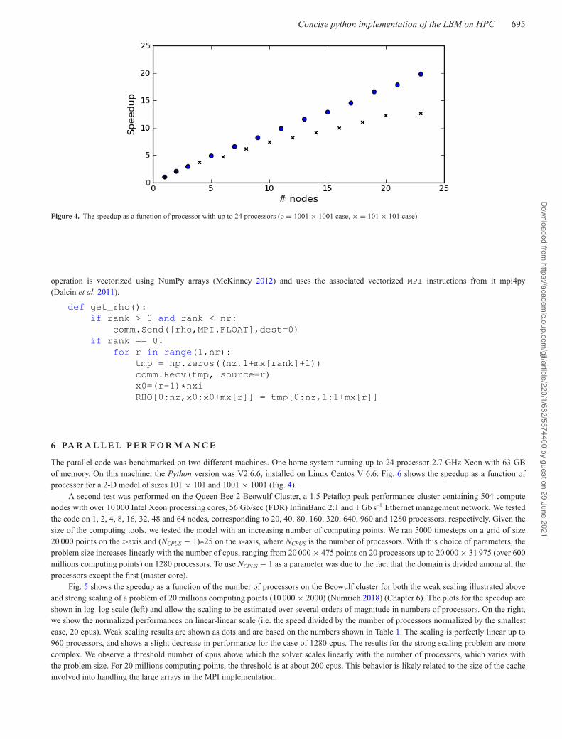
Figure 4. The speedup as a function of processor with up to 24 processors (o = 1001 × 1001 case, × = 101 × 101 case).

operation is vectorized using NumPy arrays (McKinney 2012) and uses the associated vectorized MPI instructions from it mpi4py(Dalcin et al. 2011).

6 PARALLEL PERFORMANCE

The parallel code was benchmarked on two different machines. One home system running up to 24 processor 2.7 GHz Xeon with 63 GBof memory. On this machine, the Python version was V2.6.6, installed on Linux Centos V 6.6. Fig. 6 shows the speedup as a function ofprocessor for a 2-D model of sizes 101 × 101 and 1001 × 1001 (Fig. 4).

A second test was performed on the Queen Bee 2 Beowulf Cluster, a 1.5 Petaflop peak performance cluster containing 504 computenodes with over 10 000 Intel Xeon processing cores, 56 Gb/sec (FDR) InfiniBand 2:1 and 1 Gb s–1 Ethernet management network. We testedthe code on 1, 2, 4, 8, 16, 32, 48 and 64 nodes, corresponding to 20, 40, 80, 160, 320, 640, 960 and 1280 processors, respectively. Given thesize of the computing tools, we tested the model with an increasing number of computing points. We ran 5000 timesteps on a grid of size20 000 points on the z-axis and (NCPUS − 1)∗25 on the x-axis, where NCPUS is the number of processors. With this choice of parameters, theproblem size increases linearly with the number of cpus, ranging from 20 000 × 475 points on 20 processors up to 20 000 × 31 975 (over 600millions computing points) on 1280 processors. To use NCPUS − 1 as a parameter was due to the fact that the domain is divided among all theprocessors except the first (master core).

Fig. 5 shows the speedup as a function of the number of processors on the Beowulf cluster for both the weak scaling illustrated aboveand strong scaling of a problem of 20 millions computing points (10 000 × 2000) (Numrich 2018) (Chapter 6). The plots for the speedup areshown in log–log scale (left) and allow the scaling to be estimated over several orders of magnitude in numbers of processors. On the right,we show the normalized performances on linear-linear scale (i.e. the speed divided by the number of processors normalized by the smallestcase, 20 cpus). Weak scaling results are shown as dots and are based on the numbers shown in Table 1. The scaling is perfectly linear up to960 processors, and shows a slight decrease in performance for the case of 1280 cpus. The results for the strong scaling problem are morecomplex. We observe a threshold number of cpus above which the solver scales linearly with the number of processors, which varies withthe problem size. For 20 millions computing points, the threshold is at about 200 cpus. This behavior is likely related to the size of the cacheinvolved into handling the large arrays in the MPI implementation.

Dow




Figure5.

Wea

kan

dS

tron

gS

peed

upan

dS

cali

ngs

vers

usnu

mbe

rof

proc

esso

rsup

to12

80pr

oces

sors

.Top

left

-han

dpa

nel:

log–

log

plot

ofth

esp

eedu

pfo

rth

eW

eak

scal

ing

case

.Top

righ

t-ha

ndpa

nel:

line

ar–l

inea

rpl

otof

the

norm

aliz

edpe

rfor

man

ce,a

lway

sas

sum

ing

1fo

ron

eno

de(2

0cp

us).

One

obse

rves

asl

ight

decr

ease

only

for

1280

proc

esso

rs.O

nth

ebo

ttom

the

plot

ssh

owth

esa

me

for

Str

ong

scal

ing,

i.e.s

ame

prob

lem

size

rega

rdle

ssto

the

num

ber

ofpr

oces

sors

.In

this

case

for

20m

illi

ons

com

puti

ngpo

ints

(10

000

×20

00)

the

code

star

tssc

alin

gli

near

lyfr

om16

0cp

usup

to12

80.F

ora

smal

ler

num

ber

ofpr

oces

sors

,the

reis

not

enou

ghca

che

topr

oper

lyha

ndle

the

larg

ear

rays

.

Dow




Table 1. Timing table for the weak scaling test of the parallel code, broken down to its detailed components. Times are in percentage of the total time, for theweak problem described in the test (size growing proportionally to the number of processors). The performance remains stable from 20 up to 1280 processors,with only a slight decrease in performance at 1280 processors, due to an increase in the time taken by the computational steps of the algorithm, mainly Collision.

# CpusGet edges(per cent)

Put rho bound(per cent)

Stream(per cent)

Macro(per cent)

Equilibrium(per cent)

Collision(per cent)

20 0.002 0.002 30.936 15.655 34.244 19.16240 0.001 0.001 30.776 15.625 34.316 19.28080 0.001 0.001 30.752 15.611 34.202 19.432160 0.001 0.001 30.890 15.547 34.215 19.346320 0.001 0.001 30.636 15.562 34.328 19.471640 0.002 0.002 31.099 15.477 34.528 18.892960 0.001 0.002 30.894 15.570 34.194 19.3391280 0.001 0.001 30.785 14.811 32.689 21.713

Figure 6. Performance for the parallel code, broken down in its parts, the four computational steps (Stream, Macro, Equilibrium and Collision), and thecombined cost of the two communications steps (Communication).

To understand the role of each component of the code on the performance, we compiled a detailed table with the broken down computingtime for the two communications necessary at every step (get edges() and put rho boundaries()), and of the four computing steps—(1)streaming, (2) calculation of the macroscopic properties ρ and u from the number densities fα , (3) calculation of the equilibrium numberdensities f eqα and (4) calculation and addition of the collision term � f cα . The four computing steps are respectively denoted Stream, Macro,Equilibrium and Collision. The exact timing for all of these steps for all the simulations for all the parallel tests are shown in Table 1. Themost important observation is that the time required for all the communications is several orders of magnitude smaller than the computingtime, meaning that the algorithm that we present is not prone to deadlocks or slow down for any number of processors. This can beappreciated clearly in the left-hand part of Fig. 6 where the times of the two communication steps are combined into one. This log-linear plotillustrates the orders of magnitude difference between computing and communication times, and demonstrates that communication costs arenegligible.

A more detailed look at the computing times, on the right of the Fig. 6, finally shows that the slight decrease in performance at 1280processors is due mainly to an increase in the computing time of the Collision step, and in part to the other three computing steps. Overall,the communication is optimal enough for practical uses and also for the large problems considered here.

7 APPL ICAT IONS

The code has been benchmarked with Poiseuille flow, a common test in the geodynamic literature (Gerya 2009). Fig. 7 shows that thenumerical solution matches the analytical solution on the entire domain. Towards the edges, the kink is due to the bounce-back BoundaryConditions which are at half way between lattice sites (not exactly at lattice sites).

Simulations with this code have been performed for acoustic wave propagation and for fluid flow, both in a simplified solid rock matrixmade up of circular grains and grain clusters. The matrix used for the fluid flow simulation is shown in Fig. 8 (left), and the matrix used forthe wave propagation simulation is shown on the same figure, to the right.

Dow




Figure 7. Benchmark results for the Poiseuille flow.

Figure 8. Two simplified rock matrices showing the solid region in red, and fluid region in blue. The matrix on the left is used for the porous flow simulationexample, while the one on the right is used for the wave propagation example.

Dow




Figure 9. The fluid speed after 5000 time steps in the simulation showing the fluid pathways through the rock matrix.

For the fluid-flow dynamic simulations, we have set the density of the fluid in the pore space to unity, with the left and right boundary,respectively, having a non-dimensional density of 1.01 and 0.99, respectively. These values have been chosen so that the differential density isa very small compared to the absolute magnitude. The result for speed of the fluid in the simulation after 5000 time steps is shown in Fig. 9.

It is well known that acoustic waves can propagate inside fluids in a porous medium (Lighthill 1978). The second simulation example foracoustic wave propagation is a simplified case of waves inside fluids of a porous medium. The results of the acoustic propagation simulationsare shown in Fig. 10, where a wave propagates from an initial point in nz/2, 3/4∗nx. The wave front requires about 330 steps on a resolutionof 401 × 401 to cross the entire domain and interact with the propagating wave front through periodic boundary conditions. Snapshots offluid density in the simulation in this figure are shown up to time step 400.

8 CONCLUS IONS

The LBM is a flexible computational tool that allows, among other things, one to calculate wave propagation and fluid flow in complexstrongly heterogeneous media. We show how a code developed entirely in Python displays exceptional performance, only inferior to the bestoptimized compiled C, if carefully written in a vectorized form (Morra 2018), and with the use of Just in Time compilation for selectedfunctions. Compared to C and Fortran, however, Python is easier to write (Guttag 2013), to understand, and to debug.

We also developed an MPI parallel implementation and verified that it achieves approximately linear speedup up to 24 processors ona single node of a home computer, and more relevantly for scientific applications, that it scales linearly up to at least 1280 processors ona Beowulf cluster. We therefore recommend using Python, NumPy, JiT and mpi4py for developing scientific high performance computingsoftware.

Scientific problems in geosciences that can be efficiently tackled with the LBM include fluid flow and wave propagation in porousmedia, thermochemical mantle convection, magma dynamics and volcanic eruptions. We will start off with classical 3-D mantle convectionproblems (e.g. Rabinowicz et al. 1990). Assuming that the computational time continues to scale efficiently up to 10 thousand processors ona comparable cluster to the one we used for benchmarking (10 000 Xeon processing cores, connected with 56 Gb/sec (FDR) InfiniBand 2:1),

Dow




Figure 10. Snapshots showing propagation of a wave front in a fluid with solid inclusions in the model. The algorithm captures the complexities of strongscattering from the inclusions and superposition of waves.

Dow




it will be possible to model a lattice size of 109 points (1, 0003) in about 3 minutes per 10 000 time steps. And if memory is sufficiently large,a lattice size of 1012 points (10 0003) could be calculated in about 48 hr per 10 000 time-steps. Tests on larger computing facilities are plannedand will be the topic of a follow up publication.

ACKNOWLEDGEMENTS

D.A. Yuen would like to thank National Science Foundation,s geochemistry and CISE programs for support. G. Morra would like to thankthe Board of Regents of Louisiana for support through the RCS project LEQSF(2014-17)-RD-A-14 and the Louisiana Optical NetworkInfrastructure (LONI) that provided the cluster for the test runs, through the project loni lbm01. D.A. Yuen and G. Morra would like to thankMatthew G. Knepley for the stimulating discussions on parallel scaling. The authors would like to thank the reviewers, C. Huber and C.Thieulot for helpful suggestions that improved the paper.

REFERENCESArcidiacono, S., Karlin, I., Mantzaras, J. & Frouzakis, C., 2007. Lattice

Boltzmann model for the simulation of multicomponent mixtures, Phys.Rev. E, 76, 046703.

Arun, S., Satheesh, A., Mohan, C., Padmanathan, P. & Santhoshkumar, D.,2017. A review on natural convection heat transfer problems by latticeBoltzmann method, J. Chem. Pharm. Sci., 10(1), 635–645.

Bartlett, S., 2017. A non-isothermal chemical Lattice Boltzmann Model in-corporating thermal reaction kinetics and enthalpy phase changes, Com-putation, 5(37), doi:10.3390/computation5030037.

Behnel, S., Bradshaw, R., Citro, C., Dalcin, L., Seljebotn, D.S. & Smith, K.,2011. Cython: the best of both worlds, Comput. Sci. Eng., 13(2), 31–39.

Bhatnagar, P.L., Gross, E.P. & Krook, M., 1954. A model for collisionprocesses in gases. I. Small amplitude processes in charged and neutralone-component systems, Phys. Rev., 94(3), 511.

Chen, S. & Doolen, G.D., 1998. Lattice Boltzmann method for fluid flows,Ann. Rev. Fluid Mech., 30(1), 329–364.

Dalcin, L.D., Paz, R.R., Kler, P.A. & Cosimo, A., 2011. Parallel distributedcomputing using python, Adv. Water Resour., 34(9), 1124–1139.

d’Humieres, D., Ginzberg, I., Krafczyk, M., Lallemand, P. & Luo, L.S., 2002.Multiple-relaxation-time lattice Boltzmann models in 3D, Phil. Trans. R.Soc. Lond., 360, 437–451.

Di Ilio, G., Chiappini, D., Ubertini, S., Bella, G. & Succi, S., 2017. Hy-brid lattice Boltzmann method on overlapping grids, Phys. Rev. E, 95(1),013309.

Feichtinger, C., Donath, S., Kostler, H.,Gotz,J & Rude, U., 2011. HPC de-sign software for computational engineering simulations, J. Comput. Sci.,2(2), 105–112.

Frisch, U., Hasslacher, B. & Pomeau, Y., 1986. Lattice-gas automata for theNavier-Stokes equation, Phys. Rev. Lett., 56(14), 1505.

Gerya, T., 2009. Introduction to Numerical Geodynamic Modelling. Cam-bridge Univ. Press.

Groen, D., Henrich, O., Janoschek, F., Coveney, P. & Harting, J., 2011,Lattice-Boltzmann methods in fluid dynamics: turbulance and complexcolloidal fluids, in Juelich Blue Gene/P Extreme Scaling Workshop 2011,Juelich Supercomputing Centre.

Guo, Z., Shi, B. & Zheng, C., 2002. A coupled lattice bgk model for theBoussinesq equations, Int. J. Numer. Methods Fluids, 39(4), 325–342.

Guo, J., Xing, H., Zhiwei, T. & Muhlhaus, H., 2014. Lattice Boltzmannmodeling and evaluation of fluid flow in heterogeneous porous mediainvolving multiple matrix constituents, Comput. Geosci., 62, 198–207.

Guttag, J.V., 2013. Introduction to Computation and Programming UsingPython, MIT Press.

He, X., Chen, S. & Doolen, G.D., 1998. A novel thermal model for the lat-tice Boltzmann method in incompressible limit, J. Comput. Phys., 146(1),282–300.

Heuveline, V. & Latt, J., 2007. The OpenLB project: an open source objectoriented implementation of lattice Boltzmann methods, Int. J. ModernPhys. C, 18, 627–634.

Higuera, F.J. & Jimenez, J., 1989. Boltzmann approach to lattice gas simu-lations, EPL (Europhys. Lett.), 9, 663 doi:10.1209/0295-5075/9/7/009.

Huang, H., Sukop, M. & Lu, X., 2015. Multiphase Lattice Boltzmann meth-ods: Theory and Application, John Wiley & Sons.

Huber, C., Parmigiani, A., Chopard, B., Manga, M. & Bachmann, O., 2008.Lattice Boltzmann model for melting with natural convection, Intl. J. HeatFluid Flow, 29(5), 1469–1480.

Huber, C., Shafei, B. & Parmigiani, A., 2014. A new pore-scale model for lin-ear and non-linear heterogeneous dissolution and precipitation, Geochim.Cosmochim. Acta, 124, 109–130.

Hunter, J.D., 2007. Matplotlib: a 2D graphics environment, Comput. Sci.Eng., 9(3), 90–95.

Kang, Q., Zhang, D. & Chen, S., 2003. Simulation of dissolution and precip-itation in porous media, J. geophys. Res.: Solid Earth, 108(B10), 2505–2515.

Kang, Q., Lichtner, P. & Janecky, D., 2010. Lattice Boltzmann Method forreactive flows in porous media, Adv. Appl. Math. Mech., 2, 545–563.

Keehm, Y., Mukerji, T. & Nur, A., 2004. Permeability prediction from thinsections: 3D reconstruction and Lattice-Boltzmann flow simulation, Geo-phys. Res. Lett., 31, L04606.

Kruger, T., Kusumaatmaja, H., Kuzmin, A., Shardt, O., Silva, G. & Viggen,E.M., 2017. The Lattice Boltzmann Method: Principles and Practice,Springer International Publishing.

Lagrava, D., Malaspinas, O.,Latt. J. & Chopard, B., 2012. Advances inmultidomain lattice Boltzmann grid refinement, J. Comput. Phys., 231,4808–4822.

Langtangen, H.P., Barth, T.J. & Griebel, M., 2006. Python Scripting forComputational Science, Vol. 3, Springer.

Lallemand, P. & Luo, L.S., 2000. Theory of the lattice Boltzmann method:Dispersion, dissipation, isotropy, Galilean invarience, and stability, Phys.Rev. E, 61(6), 6546–6562.

Lighthill, J., 1978. Waves in Fluids, pp. 501, Cambridge Univ. Press.Luo, L.S. & Girimaji, S., 2002. Lattice Boltzmann model for binary mix-

tures, Phys. Rev. E, 66, 035301.Lutz, M., 2013. Learning Python: Powerful Object-Oriented Programming,

O’Reilly Media, Inc.McKinney, W., 2012. Python for Data Analysis: Data Wrangling with Pan-

das, NumPy, and IPython, O’Reilly Media, Inc.Morra, G., 2018. Pythonic Geodynamics, Springer.Mora, P. & Yuen, D.A., 2017. Simulation of plume dynamics by the lattice

Boltzmann method, Geophys. J. Int., 210(3), 1932–1937.Mora, P. & Yuen, D.A., 2018a. Simulation of regimes of convection and

plume dynamics by the thermal Lattice Boltzmann Method, Phys. Earthplanet. Inter., 275, 69–79.

Mora, P. & Yuen, D.A., 2018b. Comparison of convection for Reynolds andArrhenius temperature dependent viscosities, Fluid Mech. Res. Int., 2(3),99–107.

Numrich, R.W., (2018). Parallel Programming with Co-Arrays: ParallelProgramming in FORTRAN. Chapman and Hall/CRC.

Parmigiani, A., Huber, C., Bachmann, O. & Chopard, B., 2011. Pore-scalemass and reactant transport in multiphase porous media flows, J. FluidMech., 686, 40–76.

Qian, Y., d’Humieres, D. & Lallemand, P., 1992. Lattice BGK models forNavier-Stokes equation, EPL (Europhys. Lett.), 17(6), 479.

Rabinowicz, R., Ceuleneer, G., Monnereau, M. & Rosemberg, C., 1990.Three-dimensional models of mantle flow across a low-viscosity

Dow



http://dx.doi.org/10.1103/PhysRevE.76.046703

http://dx.doi.org/10.1109/MCSE.2010.118

http://dx.doi.org/10.1103/PhysRev.94.511

http://dx.doi.org/10.1146/annurev.fluid.30.1.329

http://dx.doi.org/10.1016/j.advwatres.2011.04.013

http://dx.doi.org/10.1098/rsta.2001.0955


http://dx.doi.org/10.1016/j.jocs.2011.01.004

http://dx.doi.org/10.1103/PhysRevLett.56.1505

http://dx.doi.org/10.1002/fld.337

http://dx.doi.org/10.1016/j.cageo.2013.07.019

http://dx.doi.org/10.1006/jcph.1998.6057

http://dx.doi.org/10.1142/S0129183107010875

http://dx.doi.org/10.1016/j.ijheatfluidflow.2008.05.002

http://dx.doi.org/10.1016/j.gca.2013.09.003

http://dx.doi.org/10.1109/MCSE.2007.55

http://dx.doi.org/10.4208/aamm.10-m10S02

http://dx.doi.org/10.1016/j.jcp.2012.03.015



http://dx.doi.org/10.1093/gji/ggx279

http://dx.doi.org/10.1016/j.pepi.2018.01.003

http://dx.doi.org/10.1017/jfm.2011.268

http://dx.doi.org/10.1209/0295-5075/17/6/001


zone: implications for hotspot dynamics, Earth planet. Sci. Lett., 99,170–184.

Schornbaum, F. & Rude, U., 2016. Massively parallel algorithms for thelattice Boltzmann method on nonuniform grids, SIAM J. Scient. Comput.,28(2), C96–C126.

Shan, X., 1997. Simulation of rayleigh-benard convection using a latticeBoltzmann method, Phys. Rev. E, 55(3), 2780.

Shan, X. & Chen, H., 1993. Lattice boltzmann model for simulating flowswith multiple phases and components, Phys. Rev. E, 47(3), 1815.

Smith, K.W., 2015. Cython: A Guide for Python Programmers, O’ReillyMedia, Inc.

Succi, S., 2018. The Lattice Boltzmann Equation: For Complex States ofFlowing Matter, eds Succi, Sauro & Succi, S., Oxford Univ. Press.

Torquato, S., 2013. Random Heterogeneous Materials: Microstructure andMacroscopic Properties, Vol. 16, Springer Science & Business Media.

Van Rossum, G. et al., 2007. Python programming language, in USENIXAnnual Technical Conference, Vol. 41, p. 36.

Wang, J., Wang, D., Lallemand, P. & Luo, L.-S., 2013. Lattice Boltzmannsimulations of thermal convective flows in two dimensions, Comput.Math. Appl., 65(2), 262–286.

Xia, M., Wang, S., Shou, H., Shan, X., Chen, H., Li, Q. & Zhang, Q., 2017.Modelling viscoacoustic wave propagation with the lattice Boltzmannmethod, Scient. Rep., 7, 10169.

Xie, C., Raeini, A.Q., Wang, Y., Blunt, M.J. & Wang, M., 2017. An im-proved pore-network model including viscous coupling effects using di-rect simulation by the lattice Boltzmann method, Adv. Water Resour., 100,26–34.

Zheng, J., Ju, Y. & Wang, M., 2018. Pore-scale modeling of spontaneousimbibition behavior in a complex shale porous structure by pseudopo-tential lattice Boltzmann method, J. geophys. Res.: Solid Earth, 123,9586–9600.

Zhou, Q. & He, X., 1997. On pressure and velocity boundary conditions forthe lattice Boltzmann BGK model, Phys. Fluids, 9(6), 1591–1598.

Dow



http://dx.doi.org/10.1016/0012-821X(90)90080-H



http://dx.doi.org/10.1016/j.camwa.2012.07.001

http://dx.doi.org/10.1038/s41598-017-10833-w

http://dx.doi.org/10.1016/j.advwatres.2016.11.017

http://dx.doi.org/10.1029/2018JB016430

http://dx.doi.org/10.1063/1.869307

A concise python implementation of the lattice Boltzmann ...

Documents

Transcript of A concise python implementation of the lattice Boltzmann ...