A CASE STUDY IN PHARMACOLOGIC IMAGING USING …

Johns Hopkins University, Dept. of Biostatistics Working Papers

5-3-2007

A CASE STUDY IN PHARMACOLOGICIMAGING USING PRINCIPAL CURVES INSINGLE PHOTON EMISSION COMPUTEDTOMOGRAPHYBrian S. CaffoDepartment of Biostatistics, The Johns Hopkins Bloomberg School of Public Health, [email protected]

Ciprian M. CrainiceanuDepartment of Biostatistics, Johns Hopkins Bloomberg School of Public Health

Lijuan DengBoston Scientific Company

Craig W. HendrixJohns Hopkins School of Medicine, Division of Clinical Pharmacology

This working paper is hosted by The Berkeley Electronic Press (bepress) and may not be commercially reproduced without the permission of thecopyright holder.Copyright © 2011 by the authors

Suggested CitationCaffo, Brian S.; Crainiceanu, Ciprian M.; Deng, Lijuan; and Hendrix, Craig W., "A CASE STUDY IN PHARMACOLOGICIMAGING USING PRINCIPAL CURVES IN SINGLE PHOTON EMISSION COMPUTED TOMOGRAPHY" (May 2007). JohnsHopkins University, Dept. of Biostatistics Working Papers. Working Paper 143.http://biostats.bepress.com/jhubiostat/paper143

http://biostats.bepress.com/jhubiostat

A Case Study in Pharmacologic Imaging Using

Principal Curves in Single Photon Emission

Computed Tomography

Caffo, Brian S

Crainiceanu, Ciprian M

Deng, Lijuan

Hendrix, Craig W

May 3, 2007

Abstract

In this manuscript we are concerned with functional imaging of the colon to as-

sess the kinetics of a microbicide lubricant. The overarching goal is to understand the

distribution of the lubricant in the colon. Such information is crucial for understand-

ing the potential impact of the microbicide on HIV viral transmission. The experiment

was conducted by imaging a radiolabeled lubricant distributed in the subject’s colon.

The tracer imaging was conducted via single photon emission computed tomography

(SPECT), a non-invasive, in-vivo functional imaging technique. We develop a novel

principal curve algorithm to construct a three dimensional curve through the colon

images. The developed algorithm is tested and debugged on several difficult two di-

mensional images of familiar curves where the original principal curve algorithm does

not apply. The final curve fit to the colon data is compared with experimental sigmoi-

doscope collection.

1

Hosted by The Berkeley Electronic Press

1 Introduction

Single photon emission computed tomography (SPECT) is a non-invasive, in-vivo func-

tional imaging technique. SPECT images arise by the application of computed tomography

techniques to projections obtained by counting emitted photons from a radioactive tracer

placed in the body. SPECT images are of lower resolution than of those obtained from

other modalities, such as X-Ray CT, MRI and PET. However, SPECT represents a relatively

low-cost method for obtaining functional imaging; that is to say it offers the ability to

image the body as it functions through biological interactions with the tracer.

In this manuscript we consider functional imaging of the colon via SPECT to assess

the kinetics of a radiolabeled lubricant. The lubricant is a surrogate for a microbicide

lubricant used to prevent HIV viral transmission. Therefore, experimentally understanding

the distribution of the lubricant is crucial for understanding the potentially efficacy of such

treatments. The experiment was conducted by distributing the radiolabeled lubricant in

the colon. After introduction of the tracer, the subject was imaged in a SPECT scanner.

A second procedure was performed after scanning whereby a sigmoidoscope was used

to sample the radiolabeled lubricant at various positions within the colon. For our pur-

poses, the sigmoidoscope was a lubricated tube with an optical fiber and an additional

channel for a mechanical sampling device, which in this experiment was a brush inside a

casing. Further details on the experimental design and protocol are available on request.

Before discussing the goals of this manuscript, we briefly discuss relevant colon anatomy.

A diagram of the colon is given in Figure 1. From the anus, the next structure is the anal

canal, then rectum. The sigmoid colon follows by traveling a highly variable course anteri-

orly and slightly inferiorly from right to left where it transitions into the descending colon,

which travels up the left side of the abdomen.

A few sample transverse slices of the raw (reconstructed) image data are given in Figure

2. (A transverse plane divides the body into upper and lower regions.) As can be seen,

2

http://biostats.bepress.com/jhubiostat/paper143

Figure 1: Anatomical diagram of the colon.

Figure 2: Example raw image data axial slices. The left two show the tracer distribution in

axial slices of the descending colon while the third from the left shows distribution around

the sigmoid colon. The final plot shows the distribution near the anus.

the raw data is difficult to interpret, or to get any sort of anatomical bearings. Transverse

slices of the data having been thresholded and overlaid on the accompanying X-ray CT

image are given in Figure 3. Here the X-ray CT and SPECT are collected at the same time

and registered in the same space by the scanner software. In the top four plots, one cane

see the hip bones on the X-ray CT image and the tracer distribution in the descending

colon. The middle four plots show the tracer distribution around the lower portion of the

descending colon and the sigmoid colon, whereas the lower four plots display the tracer

near the rectum.

The primary goal of this investigation is to provide a semi-automated procedure to estimate

3


Figure 3: Processed SPECT images by transverse slices; images proceeding from the upper

left to the lower right proceed inferiorly (toward the feet). The selected images are spaced

roughly 10cm apart with each image representing a 3.45mm thick slice. For anatomical

reference, the hip bones are clearly visible in the upper left hand plots.

the concentration of the lubricant by distance in the colon using the SPECT image. With

reliable information from the imaging data, the sigmoidoscope collection would not be

necessary in future studies. In addition, the sigmoidoscope itself displaces the liquid, hence

has limitations for measuring the tracer distribution.

To solve the problem, we develop a algorithm based on principal curves (Hastie and

Stuetzle, 1989) to perform the fitting. The resulting algorithm incorporates constrained

endpoints (of the curve), constrained interior points and the image intensities. Moreover,

a novel “warming-up” procedure is given that greatly improves the ability of the algorithm

to fit complex data structures. The algorithm was tested and debugged on a collection

of difficult two dimensional (2D) images that the original, unmodified, principal curve

4


algorithm could not fit.

With one subject, the scientific contribution of this work is largely a proof of concept.

However, it will be shown that the algorithm appears to work quite well and requires little

user input. The excellent results of the algorithm have lead to the potential policy change

of eliminating the costly and invasive sigmoidoscope collection.

The article is organized as follows. Section 2 overviews the data. Section 3 covers curve

fitting algorithms, beginning with a literature review. Subsection 3.1 covers curve charac-

terizations while 3.2 discusses principal curves while our modified algorithm is discussed

in 3.3. Section 4 tests these algorithms on constructed 2-D data, while the algorithms are

applied to the real SPECT data in Section 5. The manuscript concludes with a discussion

in Section 6.

2 Data

Ten milliliters of radiolabeled lubricant (99 m TC-sulfur colloid mixed with K-Y Jelly R© John-

son and Johnson, New Brunswick, NJ) were injected into the subject’s colon. Following

rectal administration of the radiolabeled gel, the subject underwent simulated receptive

anal intercourse. The experimental paradigm was designed to mimic the typical forces

that would influence the lubricant’s distribution.

Subsequently, the patient was imaged on a dual-head VG SPECT-CT imaging system

(GE Medical Systems, Waukesha, WI) equipped with a low-end computed tomography

(CT) unit (Hawkeye). Accompanying each SPECT image, an X-ray computed tomogra-

phy image was also collected for anatomical reference and reconstruction of the SPECT

image. The image was reconstructed using the ordered subsets EM algorithm (Hudson

and Larkin, 1994) and filtered as provided with the scanner software (General Electric

eNTEGRA workstation, version 1.04, GE Medical Systems, Waukesha, WI).

The SPECT data is represented as a three dimensional array. In our application the

5


dimension of the array is 128× 128× 128. Each voxel (three dimensional pixel) represents

a 3.45 mm3 physical area. The image intensity values are proportional to the concentration

of the tracer at that location. The intensity values range from 0 to 187, though we note that

the absolute scale is somewhat arbitrary, as the image was rescaled during reconstruction.

After imaging, a sigmoidoscope was used to collect physical concentration measure-

ments. Samples were taken at 5cm intervals up to 40cm. The study was approved by the

Johns Hopkins Institutional Review Board and informed written consent was given.

3 Curve fitting algorithms

Calculating centerlines for anatomical structures such as blood vessels, neurons or colons

has a rich history in the computer vision and medical image processing literature. Much

of the research involving colons are applied to X-ray CT images for the purposes of finding

polyps. For example, McFarland et al. (1997) present a semi-automated centerline extrac-

tion algorithm. Samara et al. (1998) proposed a semi-automated voxel search algorithm

for centerline construction.

Another class of methods employ Dijkstra’s algorithm (see Dijkstra, 1959), where vox-

els and intensity values are treated as a networked graph. Search algorithms are used

to find minimal distance paths through the graph (Chiou et al., 1998; Bitter et al., 2001;

Hong et al., 1997). Wan et al. (2001) uses distance fields to compute central paths, while

Chaudhuri et al. (2004) used similar concepts, but with a different distance measure. Co-

hen and Kimmel (1997) derived a path tracking routine in two dimensional images by

calculating a minimal path between two fixed end points.

Deschamps and Cohen (2001) extended the so-called fast marching algorithm to three

dimensional objects to extract a minimal path through the colon. Ge et al. (1999) use a

fast topological thinning algorithm to generate a three dimensional skeleton of a binary

colon volume, which is subsequently pruned. Bouix et al. (2003) uses a technique called

6


medial surface extraction to compute a centerline curve, which is then pruned. Finally,

Telea and Vilanova (2003) give a level-set algorithm for building a colon centerline.

After having mentioned only a subset of the related work on calculating colon cen-

terlines, we emphasize that our problem differs markedly from these approaches in sev-

eral important ways. First, this work considers SPECT images rather than high resolution

anatomical X-ray CT images. Furthermore, the image is of the tracer/lubricant mixture,

not of colon anatomy. The tracer may be at lower concentrations at different areas of

the colon, where the centerline is still desired, so that image intensities are not the pri-

mary concern (as opposed to the analysis of X-ray CT images). Moreover, unlike the colon

anatomy, the tracer distribution can be discontinuous, interrupted by stool and gas. There-

fore, techniques requiring connected graphs would not apply. It also worth emphasizing

that the scientific application is extremely novel, with no comparable experiments. In

addition, there is a direct comparison measurement available in the sigmoidoscope data.

Finally, largely due to the authors’ backgrounds, our approach and characterization of the

problem is more statistically oriented than existing algorithms.

Statistical approaches in the area of curve fitting are few - as opposed to the embar-

rassment of riches available for fitting proper functions. Below we discuss the principal

curve algorithm, a fundamental algorithm in the area of curve fitting. However, we found

that, unmodified, this algorithm could not handle complex images. Moreover, it does not

incorporate image intensities. Therefore we proposed a modified algorithm with several

notable benefits.

3.1 Characterization of curves

We characterize the problem as follows. Let f : R → R3 be defined so that f(t) =

{fx(t), f y(t), f z(t)} = {X(t), Y (t), Z(t)}. Here, f is the three dimensional position of a

curve through the colon at a latent argument t ∈ [0, 1]. The value of f(t) represents the

coordinate points in the image; hence, the curve in three dimensional space is then the

7


Figure 4: Sampled colon images in two orientations. Colors represent image intensity.

projection of f(t) over t. As such, this is a standard representation of a curve in (see

Thorpe, 1979, for example). The constraint that t resides in [0, 1] is arbitrary, and used

for identifiability. Throughout we conceptualize f(t) as the position of a curve at a “time

point” t. We emphasize that this is only for pedagogy; the image has no temporal compo-

nent. Conceptually considering time highlights the identifiability issue that two functions

traveling the same path at different rates yield the same curve.

The general requirements for the fitted curve are: i) the curve should follow a smooth

path through the center of the tracer distribution, ii) the curve must be able to traverse

empty spaces, where the continuity of the tracer is interrupted, iii) using the X-ray CT

image landmarks, user specified starting and ending points should be incorporated, iv) the

algorithm should be flexible enough to allow for other user specified points that the curve

must travel through and v) the curve should prefer traversing higher intensity points to

lower. We note that point v) must be considering delicately, as excessively emphasizing

the image intensities can result in poor fits. Consider the example data, where the highest

intensity points are aggregated near the anus. Any algorithm that minimizes the curve in-

tegral of the intensities through the image will focus on spending as much time as possible

8


in these areas, contrary to goals i) and ii).

To achieve these requirements we build on the principal curve algorithm of Hastie and

Stuetzle (1989). Our modifications were borne out of difficulty in getting reasonable fits

out of the original algorithm for challenging imaging problems and the fact that it was not

designed to incorporate image intensity values. Our approach does require user-specified

endpoints for the curve, mostly because of the nature of the scientific problem. However,

a novel warm-up procedure automates the selection of a starting curve, starting at a line

connecting the two specified endpoints and gradually capturing finer details of the curve.

Moreover we provide an elegant solution to accounting for differences in image intensity

that does not suffer from the problems outlined above.

We describe the principal curve algorithm and our modifications in the next two sec-

tions. However, before a discussion of the algorithms, we discuss necessary preprocessing

and some basic starting points for curve fitting through images.

A first step is to threshold the image. This is done both to remove background noise

and to reduce the number of points included in the fitting. Further acceleration is obtained

randomly sampling points that survive the threshold. Points should be sampled uniformly

among those that are above the threshold. Sampling points with probabilities relative to

image intensities gives poor results.

Notationally, let {(Xi, Yi, Zi)}ni=1 be the sampled locations. To be specific, (Xi, Yi, Zi)

represents the lattice value of a single sampled point above the original threshold. The

index ordering, i, is arbitrary; that is the points can be selected in any order. Figure 4

shows the sampled colon data. Let {ti}ni=1 represent a collection of (unknown) associated

time variables for the sampled points. Throughout, dropping the subscript will represent

the vector of the collection of variables, such as t = (t1, . . . , tn)′.

Much of the challenge of this problem is to appropriately assign values for the time

points. Tabling this issue for the moment, presume that these points were known. Then a

9


smooth curve through the data could be easily fit using three spline equations:

E[Xi] = fx(ti) = βx0 + βx

1 ti + βx2 t2i + βx

3 t3i +K∑

k=1

bxk(ti − ξk)

3+,

E[Yi] = f y(ti) = βy0 + βy

1 ti + βy2 t

2i + βy

3 t3i +

K∑k=1

byk(ti − ξk)

3+, (1)

E[Zi] = f z(ti) = βz0 + βz

1ti + βz2t

2i + βz

3t3i +

K∑k=1

bzk(ti − ξk)

3+,

where {ξk}Kk=1 are knots placed at equally spaced quantiles of {ti}n

i=1. Here K + 4 is the

degrees of freedom of the smoother for each dimension. The benefits of using regres-

sion splines are many, including the easy specification of the basis and the easily derived

derivatives, which are required later.

3.2 Principal curves

The principal curve algorithm (Hastie and Stuetzle, 1989) is a general method for fitting a

curve through data residing in an arbitrary dimensional space. A curve, f(t), is said to be

a principal curve if for each data value, say (Xi, Yi, Zi), the curve at ti satisfies

f(ti) = E[(Xi, Yi, Zi) | closest point of f to (Xi, Yi, Zi) occurred at time = ti].

This recursive form of self consistency motivates an algorithm. Suppose that a starting

collection of time points is given.

1. Approximate the principal curve by a scatterplot smoother, regressing {(Xi, Yi, Zi)}ni=1

on {ti}ni=1 [as in Equation (1)].

2. Update the time points by redefining ti as the time point on the curve closest to

(Xi, Yi, Zi) for i = 1, . . . , n. That is, define

ti = argmint∈[0,1]

√{Xi − fx(t)

}2

+{

Yi − f y(t)}2

+{

Zi − f z(t)}2

for i = 1, . . . , n, where fx(t), for example, represents the current estimate of fx(t).

10


These steps are then iterated until convergence. Of course, instead of a starting at a

collection of time points, a starting curve could be given, in which case the algorithm

simply starts at Step 2. For example, one could start the algorithm at the first principal

component line through the data. In our setting, we start algorithm at a line connecting

user-specified endpoints.

Conceptually the steps can be thought of as the following. First the data is projected

onto the three planes considering time and each spatial dimension. That is, the data

(t,X), (t, Y ) and (t, Z) are considered; where, for example, (t,X) refers to the collection

of {ti}ni=1 and {Xi}n

i=1 data points. Secondly, a scatterplot smoother is fit in those three

planes to calculate an updated curve. Next, the orthogonal projections of the data points

onto the curve are calculated. The time points associated with the projections onto the

curve are used to then update the latent time variable. While this strategy has considerable

intuitive appeal, a formal proof of convergence is not available. However, it has been used

successfully in (unrelated) image processing settings (Banfield and Raftery, 1992).

3.3 A modified principal curve algorithm

In this section we discuss generalizations of the principal curve algorithm that allow it to

be viable in our scientific setting. These modifications are: allowing for user-specified end-

points and interior points of the function, incorporating the image intensities, warming-up

the algorithm to achieve better fit, a grid search to perform the minimization in the second

step of the algorithm and a stopping rule based on relative mean squared error.

Consider the incorporation of user-specified endpoints. Notationally suppose that (x0, y0, z0)

and t0 = 0 and (xn+1, yn+1, zn+1) and tn+1 = 1 are given. A modification of the algorithm

that forces the curve to start and end at these points (respectively), simply forces the con-

straint 0 ≤ ti ≤ 1 for i = 1, . . . , n and adds the relevant Lagrange multiplier terms to

Equation (1). That is, the multiplier terms force fx(0) = x0, fx(1) = xn+1, f y(0) = y0,

f y(1) = yn+1, f z(0) = z0, f z(1) = zn+1. Specifically, let W be the basis matrix for Equation

11


(1) (note the same basis is used for all three dimensions). Let W be the basis evaluated at

the constrained values of t and let x, y and z be vectors of the constrained values. Then

the goal is to maximize the equations

E[X] = Wβx E[Y ] = Wβy E[Z] = Wβz

subject to the constraints

Wβx = x Wβy = y W βz = z.

The fitted values are then (see Searle, 1971, for example)

βxc = βx − (W ′W )−1W{W ′(W ′W )−1}−1(W βx − x),

βyc = βy − (W ′W )−1W{W ′(W ′W )−1}−1(W βy − y), (2)

βzc = βz − (W ′W )−1W{W ′(W ′W )−1}−1(W βz − z),

where βx, βy and βz are the unconstrained fitted coefficients.

It is worth noting that constraining the endpoints as such implies that the end fitted

curve will not satisfy the self consistency property. In particular, points near the fixed

endpoints will not have their values of t updated by the orthogonal projection to the curve

extended in perpetuity, but instead by the closest value to the constrained ends.

This solution can be adapted to incorporate other constrained points along the curve.

However, unlike the endpoints, the corresponding values of ti are not known. Therefore,

these associated time points must be estimated in Step 2 of the principal curve algorithm

and the matrix of constrained time points, W , must be updated. We note that this proce-

dure must be used with care, as identifiability problems can occur with constrained interior

points. A minimum requirement is that there generally needs to be more parameters than

constrained points. For example, one cannot constrain a line to traverse three points unless

those points fall on a line.

Consider incorporating the image intensities. Specifically, define Σ−1 to be a matrix

with some function of the image intensities corresponding to the points {(Xi, Yi, Zi)}ni=1

12


along the main diagonal and zeros elsewhere. Then consider the weighted regression

version of Equation 2

βxc = βx − (W ′Σ−1W )−1W{W ′(W ′Σ−1W )−1}−1(W βx − x),

βyc = βy − (W ′Σ−1W )−1W{W ′(W ′Σ−1W )−1}−1(W βy − y),

βzc = βz − (W ′Σ−1W )−1W{W ′(W ′Σ−1W )−1}−1(W βz − z),

where now βx, βy and βz are the unconstrained weighted fitted coefficients. For example,

βx = (W ′Σ−1W )−1W ′Σ−1X.

Note that the fit is invariant to scalings of the image intensities. Though we used the

raw image intensities to define Σ−1, other definitions could be used to adapt the fit. For

example, using the square of the intensities will put greater emphasis on high intensity

points while using the square root will put less. Users of the algorithm should be advised

that it may be useful to trim the intensities to avoid excessive impact for outlying points.

This was not necessary in our application.

The most important modification of the principal curve algorithm lies in choosing an

appropriate starting curve. We have found that getting the curve in the correct neigh-

borhood is crucial for fitting complicated structures. Therefore, we employ a series of

warm-up runs, using few degrees of freedom (small K) to obtain starting values that cor-

rectly model the gross features of the data. We start the warm-up runs at a line connecting

the two specified endpoints. For each value of K, the modified principal curve algorithm

could then be run to convergence. After convergence, the estimated curve is then used as

a starting value for a subsequent warm-up run of the algorithm with K increased. A final

run with the desired value of K uses the result of the warm-up runs as the starting value.

This method tends to mold the curve to the gross features of the data before moving on

to the finer ones. We have found that this is the single most important aspect of obtaining

reasonable fits. Furthermore, the most critical aspect of using these warm-up runs is sys-

tematically increasing the degrees of freedom. Whether or not the algorithm is run until

13


Figure 5: Sample images.

convergence within each warm-up value of K does not seem to impact results, other than

slowing the algorithm down. Therefore, only one iteration within value of K was used to

warm-up to the final run.

Two algorithms were attempted to perform the maximization required in Step 2 of the

principal curve algorithm. First, a modified BFGS algorithm was used that can accom-

modate constrained endpoints (Byrd et al., 1995). Secondly, a simple grid search was

also used. Both techniques were effective, though the grid search was quite a bit faster.

Therefore, the results presented employed that technique using 1, 000 or 10, 000 grid points

between 0 and 1. All calculations were performed in the R programming language (R De-

velopment Core Team, 2006).

With regard to stopping the algorithm, we used the relative change in the mean squared

error of the estimated function summed across the three dimensions. Specifically, define

SMSE =1

n

n∑i=1

[{Xi − fx(ti)}2 + {Yi − f y(ti)}2{Zi − f z(ti)}2],

and hence the stopping criteria required

|SMSEcurrent − SMSEold|SMSEold

to be less than a desired tolerance.

14


Figure 6: Fitted images for the spiral. In the top panel the line interpolating the two (blue)

specified endpoints is given where the bottom plots the fits after being run to twenty

degrees of freedom. The first plots on the left show the fitted curve. The second shows the

data and the fitted curve, first projected onto the (X,Y ) plane and secondly the full data

with the unobserved variable t. The latter two plots show the (t,X) and (t, Y ) projections

of the data and the fitted curve.

4 Idealized 2-D curves

To build intuition, the algorithm was applied to highly idealized two dimensional images

created using image processing software. Figure 5 displays the raw images. Note they are

of constant intensity, hence the weight matrix, Σ−1, was set to an identity matrix. These

images were selected as they possess several interesting features, such as sharp turns, and

are quite a bit more difficult to fit than the actual data set. Many of these test images were

motivated by Kegl et al. (2000). The 512 × 512 pixel images were created in the GIMP

(GNU Image Manipulation Program, www.gimp.org) by freehand drawing with a mouse.

15


Figure 7: Results of fits, not employing warm-up runs, overlaid on the sampled data. The

left plot shows the results with constrained endpoints while the right plot shows the fit

without any constraints starting at the principal component line.

Figure 6 shows the sample fitted curves to the spiral using K = 20 to define the degrees

of freedom (bottom plots) from several orientations, as well as the starting line (top plots).

The fixed endpoints are shown as blue points. The leftmost plots show the fitted curve.

The next to the right show the (X, Y, t) data and the fitted curve in three dimensional

space with the (X, Y ) data shown projected onto the plane. The next panels show the

(t,X) and (t, Y ) data and the fitted curve projections. Recall that the smoothing portion

of the algorithm fits a smoother to these two projections.

The same plots for the other examples are given in Figure 11. In all of the cases, the

fit is obviously good. Because of the sampling and the fast grid-search maximization, the

algorithms take only roughly thirty seconds to run. Also, the process of warming-up the

fit tends to get the curve in a very close neighborhood of the desired limit, thus requiring

very few iterations for the final run.

To further emphasize the utility of the warm up runs, Figure 7 shows sampled data from

the spiral and the overlaid fits - without using the warm up runs - after three iterations with

16


Figure 8: Results of model fits to the “3” and spiral using constrained interior points of the

function. The constrained interior points are in green while the constrained endpoints are

shown in blue.

k = 20. In both cases the curve is struggling to hit as many points as possible to minimize

the orthogonal projections onto the curve. The curve does not have the ability to fit gross

features and so immediately takes as complex as a shape as possible. This problem could

be overcome by starting the curve using several constrained interior points, as described in

Section 3.3, then perhaps one could quickly discard them, as a few iterations would place

the curve in the right neighborhood. However, this would require excessive user input

and the warm-up procedure seems to largely avoid this problem in an automated fashion.

Below, we discuss the use of constrained interior points when employing the warm-up

runs.

Figure 8 shows the results of the fitted models employing constrained interior points

that the functions must traverse (shown in green). Here K = 20 was used to define the fi-

nal degrees of freedom of the smoothers. For the “3” image, the constrained interior points

were nicely incorporated into the smooth curve. In contrast, for the spiral, the constrained

interior points interfered with the fit, forcing the curve to make unnatural bends to incor-

17


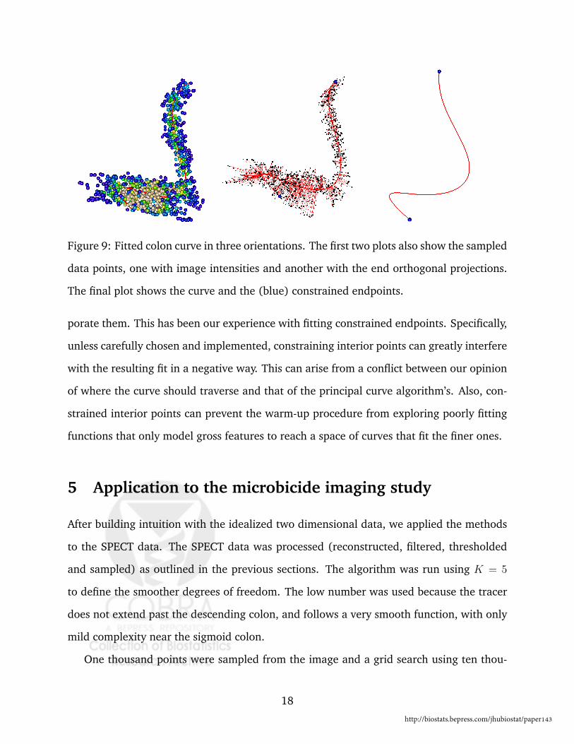
Figure 9: Fitted colon curve in three orientations. The first two plots also show the sampled

data points, one with image intensities and another with the end orthogonal projections.

The final plot shows the curve and the (blue) constrained endpoints.

porate them. This has been our experience with fitting constrained endpoints. Specifically,

unless carefully chosen and implemented, constraining interior points can greatly interfere

with the resulting fit in a negative way. This can arise from a conflict between our opinion

of where the curve should traverse and that of the principal curve algorithm’s. Also, con-

strained interior points can prevent the warm-up procedure from exploring poorly fitting

functions that only model gross features to reach a space of curves that fit the finer ones.

5 Application to the microbicide imaging study

After building intuition with the idealized two dimensional data, we applied the methods

to the SPECT data. The SPECT data was processed (reconstructed, filtered, thresholded

and sampled) as outlined in the previous sections. The algorithm was run using K = 5

to define the smoother degrees of freedom. The low number was used because the tracer

does not extend past the descending colon, and follows a very smooth function, with only

mild complexity near the sigmoid colon.

One thousand points were sampled from the image and a grid search using ten thou-

18


0 10 20 30 40

0.0

0.2

0.4

0.6

0.8

1.0

Distance (CM)

Con

cent

ratio

n / m

ax(C

once

ntra

tion)

Sigmoidoscope1248

Figure 10: Concentration estimates by distance (in centimeters) from the curve beginning

(near the anus) using various neighborhood sizes around the curve. The sigmoidoscope

data is shown in black. All curves are normalized relative to their maximum value.

sand equally spaced points between zero and one were employed in the second step of

the principal curve algorithm. The modified BFGS algorithm was also employed, though

it demonstrated no difference in results. The constrained endpoints were selected by com-

parisons with bone structure from the X-ray CT image. No constrained interior points were

necessary, as the lubricant distribution is fairly continuous.

Figure 9 shows the fit in three orientations, two of which display the sampled data, on

with the image intensities and the other with the orthogonal projections onto the curve.

The shape of the curve was evaluated by physicians, who claimed it closely followed prior

19


knowledge regarding colon anatomy.

The fitted curve was compared with the sigmoidoscope results. The distance along the

curve was calculated as ∫ T

0

√d

dtfx(t)2 +

d

dtf y(t)2 +

d

dtf z(t)2dt,

where fx(t), for example, denotes the final estimate for fx(t). Because of the simple form

for the basis used, f has an easily calculated derivatives. We did not, however, find a closed

form for the resulting integral, which was evaluated numerically. Image intensities were

then calculated along the curve using the original, unsampled, image, in neighborhoods

of size 1, 2, 4 and 8 voxels. Here a neighborhood of size c is defined as the box centered at

the current voxel with sides (2c + 1). The concentration was estimated as the sum of the

image intensities in the neighborhood, divided by the number of number of voxels.

Figure 10 displays the results as well as the sigmoidoscope data for comparison. Since

image processing arbitrarily scales the reconstructed SPECT image, the intensities used

in the concentration calculation are only proportional to the actual tracer concentration.

Therefore, all of the curves were divided by their maximum value, to obtain a unit-free

comparison.

At a first glance, there appears to be little agreement with the sigmoidoscope. However,

the starting distance of the two images are not calibrated. That is, it is not known how

far into the colon the SPECT image starts. If the SPECT images are shifted 10 − 20 cm

to the right, then the agreement is very good. Therefore, a clear limitation of the SPECT

method is the lack of an accurate starting distance. However, unlike the sigmoidoscope, the

SPECT image can reasonably detect the tracer distribution will into the colon. In addition,

the sigmoidoscope displaces the tracer/lubricant mixture during sampling. As such, the

image processing tools presented offer an extremely valuable source of quantification of

the tracer/lubricant distribution without this source of error. Currently the authors are

working with scientific collaborators to obtain accurate measures of the starting distance

of the tracer distribution in the SPECT image.

20


6 Discussion

In this manuscript we consider the difficult problem of three dimensional curve fitting

in a novel, scientifically important, study. The success of the algorithm has inspired the

possibility that the costly and invasive sigmoidoscope collection can be abandoned and

replaced by statistical image processing tools, provided an accurate measure of the starting

distance of the tracer distribution from the anus.

The developed algorithm proved to be an ideal candidate for obtaining a centerline

through the distribution of the SPECT tracer. Techniques for constraining endpoints and

interior points were given. Furthermore, in the challenging 2-D test images, the single

most important modification was clearly the warm-up procedure, where lower smoothing

degrees of freedom were used the capture gross features of the data before moving on to

the finer ones.

While this research has provided scientific collaborators with a set of easily imple-

mentable tools for processing their images and obtaining concentration/distance curves,

the larger, more general, problem of arbitrary dimensional curve fitting leaves much room

for further methodological development. We have found that this collection of problems,

while considered in the image processing literature, has received insufficient attention in

the statistics literature. We conjecture that better adaptive smoothing procedures may be

required to fit more complicated images. Furthermore, a greater degree of automation

for the procedures would be beneficial to users. Finally, though the developed algorithm

proved to be very successful in this application, other methods for allocating the time

points could be considered in other settings. For example, Deng (2007) considered a

stochastic search algorithm under a user specified objective function.

21


References

Banfield, J. and Raftery, A. (1992). Ice Floe Identification in Satellite Images Using Math-

ematical Morphology and Clustering about Principal Curves. Journal of the American

Statistical Association, 87(417).

Bitter, I., Kaufman, A., and Sato, M. (2001). Penalized-distance volumetric skeleton algo-

rithm. IEEE Trans Vis Comp Graph, 7:195–206.

Bouix, S., Siddiqi, K., and Tannenbaum, A. (2003). Flux driven fly throughs. In 2003

conference on Computer Vision and Patern Recognition (CVPR 2003), pages 449–454.

Byrd, R., Lu, P., Nocedal, J., and Zhu, C. (1995). A limited memory algorithm for bound

constrained optimization. SIAM Journal on Scientific Computing, 16(5):1190–1208.

Chaudhuri, P., Khandekar, R., Sethi, D., and Kalra, P. (2004). An efficient central path algo-

rithm for virtual navigation. Proceedings of the Computer Graphics International (CGI’04),

00:188 – 195.

Chiou, R., Kaufman, A., Liang, Z., Hong, L., and Achniotou, M. (1998). Interactive path

planning for virtual endoscopy. In Proc. of the IEEE Nuclear Science and Medical Imaging

Conference.

Cohen, L. and Kimmel, R. (1997). Global minimum for active contour models: A minimal

path approach. Journal of Computer Vision, 24 (1):57–78.

Deng, L. (2007). Spline-based curve fitting with applications to kinetic imaging. Master’s

thesis, Department of Biostatistics, Johns Hopkins University.

Deschamps, T. and Cohen, L. (2001). Fast extraction of minimal paths in 3d iamges and

applications to virtual endoscopy. Medical Image Analysis, 5:281–299.

22


Dijkstra, E. (1959). A note on two problems in connexion with graphs. Numerische Math-

ematik, 1:269–271.

Ge, Y., Stels, D., Wang, J., and Vining, D. (1999). Computing centerline of a colon: A robust

and efficient method based on 3d skeletons. Journal of Computer Assisted Tomography,

23(5):786–794.

Hastie, T. and Stuetzle, W. (1989). pincipal curves. Journal of the American Statistical

Association.

Hong, L., Muraki, S., Kaufman, A., Bartz, D., and He, T. (1997). Virtual voyage: Interactive

navigation in the human colon. In Proc. of SIGGRAPH’97.

Hudson, H. M. and Larkin, R. S. (1994). Accelerated image reconstruction using ordered

subsets projection data. IEEE Transactions on Medical Imaging, 13:601–609.

Kegl, B., Krzyzak, A., Linder, T., and Zeger, K. (2000). Learning and design of principal

curves. Pattern Analysis and Machine Intelligence, IEEE Transactions on, 22(3):281–297.

McFarland, E., Wang, G., Brink, J., Balfe, D., Heiken, J., and Vannier, M. (1997). Spi-

ral computed tomographic colonography: Determination of the central axis and digital

unraveling of the colon. Acad Radiol, 4:367–373.

R Development Core Team (2006). R: A Language and Environment for Statistical Comput-

ing. R Foundation for Statistical Computing, Vienna, Austria. ISBN 3-900051-07-0.

Samara, Y., Fiebich, M., Dachman, A., Doi, K., and K., H. (1998). Automated centerline

tracking of the human colon. In Proc. of the SPIE Conference on Image Processing.

Searle, S. (1971). Linear Models. Wiley.

Telea, A. and Vilanova, A. (2003). A robust level-set algorithm for centerline extraction.

In Proceedings of the symposium on Data visualisation 2003, pages 185–194.

23


Thorpe, J. (1979). Elementary Topics in Differential Geometry. Springer-Verlag, New York.

Wan, M., Dachille, F., and A., K. (2001). Distance-field based skeletons for virtual naviga-

tion. In IEEE Visualization 2001, pages 239–245.

24


Figure 11: Fitted values for three example data sets at 20 degrees of freedom.

25


A CASE STUDY IN PHARMACOLOGIC IMAGING USING …

Documents

Transcript of A CASE STUDY IN PHARMACOLOGIC IMAGING USING …