A BRIEF INTRODUCTION TO SPECTRAL GRAPH THEORY · 2 A BRIEF INTRODUCTION TO SPECTRAL GRAPH THEORY...
92
arXiv:1609.08072v1 [math.CO] 26 Sep 2016 A BRIEF INTRODUCTION TO SPECTRAL GRAPH THEORY BOGDAN NICA –I NTRODUCTION – Spectral graph theory starts by associating matrices to graphs, notably, the adja- cency matrix and the laplacian matrix. The general theme is then, firstly, to compute or estimate the eigenvalues of such matrices, and secondly, to relate the eigenval- ues to structural properties of graphs. As it turns out, the spectral perspective is a powerful tool. Some of its loveliest applications concern facts that are, in principle, purely graph-theoretic or combinatorial. To give just one example, spectral ideas are a key ingredient in the proof of the so-called Friendship Theorem: if, in a group of people, any two persons have exactly one common friend, then there is a person who is everybody’s friend. This text is an introduction to spectral graph theory, but it could also be seen as an invitation to algebraic graph theory. On the one hand, there is, of course, the linear algebra that underlies the spectral ideas in graph theory. On the other hand, most of our examples are graphs of algebraic origin. The two recurring sources are Cayley graphs of groups, and graphs built out of finite fields. In the study of such graphs, some further algebraic ingredients (e.g., characters) naturally come up. The table of contents gives, as it should, a good glimpse of where is this text going. Very broadly, the first half is devoted to graphs, finite fields, and how they come together. This part is meant as an appealing and meaningful motivation. It provides a context that frames and fuels much of the second, spectral, half. Most sections have one or two exercises. Their position within the text is a hint. The exercises are optional, in the sense that virtually nothing in the main body depends on them. But the exercises are often of the non-trivial variety, and they should enhance the text in an interesting way. The hope is that the reader will enjoy them. We assume a basic familiarity with linear algebra, finite fields, and groups, but not necessarily with graph theory. This, again, betrays our algebraic perspective. This text is based on a course I taught in Göttingen, in the Fall of 2015. I would like to thank Jerome Baum for his help with some of the drawings. The present version is preliminary, and comments are welcome (email: [email protected]). Date: September 27, 2016. 1
Transcript of A BRIEF INTRODUCTION TO SPECTRAL GRAPH THEORY · 2 A BRIEF INTRODUCTION TO SPECTRAL GRAPH THEORY...

arX
iv:1
609.
0807
2v1
[m
ath.
CO
] 2
6 Se
p 20
16
A BRIEF INTRODUCTION TO SPECTRAL GRAPH THEORY
BOGDAN NICA
– INTRODUCTION –
Spectral graph theory starts by associating matrices to graphs, notably, the adja-cency matrix and the laplacian matrix. The general theme is then, firstly, to computeor estimate the eigenvalues of such matrices, and secondly, to relate the eigenval-ues to structural properties of graphs. As it turns out, the spectral perspective is apowerful tool. Some of its loveliest applications concern facts that are, in principle,purely graph-theoretic or combinatorial. To give just one example, spectral ideas area key ingredient in the proof of the so-called Friendship Theorem: if, in a group ofpeople, any two persons have exactly one common friend, then there is a person whois everybody’s friend.
This text is an introduction to spectral graph theory, but it could also be seen asan invitation to algebraic graph theory. On the one hand, there is, of course, thelinear algebra that underlies the spectral ideas in graph theory. On the other hand,most of our examples are graphs of algebraic origin. The two recurring sources areCayley graphs of groups, and graphs built out of finite fields. In the study of suchgraphs, some further algebraic ingredients (e.g., characters) naturally come up.
The table of contents gives, as it should, a good glimpse of where is this textgoing. Very broadly, the first half is devoted to graphs, finite fields, and how theycome together. This part is meant as an appealing and meaningful motivation. Itprovides a context that frames and fuels much of the second, spectral, half.
Most sections have one or two exercises. Their position within the text is a hint.The exercises are optional, in the sense that virtually nothing in the main bodydepends on them. But the exercises are often of the non-trivial variety, and theyshould enhance the text in an interesting way. The hope is that the reader will enjoythem.
We assume a basic familiarity with linear algebra, finite fields, and groups, butnot necessarily with graph theory. This, again, betrays our algebraic perspective.
This text is based on a course I taught in Göttingen, in the Fall of 2015. I wouldlike to thank Jerome Baum for his help with some of the drawings. The presentversion is preliminary, and comments are welcome (email: [email protected]).
Date: September 27, 2016.
1
2 A BRIEF INTRODUCTION TO SPECTRAL GRAPH THEORY
CONTENTS
– Introduction – 11. Graphs 4Notions 4Bipartite graphs 72. Invariants 9Chromatic number and independence number 9Diameter and girth 10Isoperimetric number 123. Regular graphs I 14Cayley graphs 14Vertex-transitive graphs 17Bi-Cayley graphs 194. Regular graphs II 20Strongly regular graphs 20Design graphs 225. Finite fields 23Notions 24Projective combinatorics 25Incidence graphs 276. Squares in finite fields 28Around squares 28Two arithmetic applications 30Paley graphs 33A comparison 367. Characters 38Characters of finite abelian groups 38Character sums over finite fields 40More character sums over finite fields 43An application to Paley graphs 448. Eigenvalues of graphs 46Adjacency and laplacian eigenvalues 46First properties 48First examples 509. Eigenvalue computations 52Cayley graphs of abelian groups 52Bi-Cayley graphs of abelian groups 53Strongly regular graphs 55Two applications 56Design graphs 57Partial design graphs 5810. Largest eigenvalues 60Extremal eigenvalues of symmetric matrices 60Largest adjacency eigenvalue 62The average degree 64A spectral Turán theorem 65Largest laplacian eigenvalue of bipartite graphs 67Subgraphs 68

A BRIEF INTRODUCTION TO SPECTRAL GRAPH THEORY 3
Largest eigenvalues of trees 7011. More eigenvalues 74Eigenvalues of symmetric matrices: Courant - Fischer 74A bound for the laplacian eigenvalues 75Eigenvalues of symmetric matrices: Cauchy and Weyl 77Subgraphs 7912. Spectral bounds 81Chromatic number and independence number 81Isoperimetric constant 83Edge-counting 88– Further reading – 92

4 A BRIEF INTRODUCTION TO SPECTRAL GRAPH THEORY
1. GRAPHS
Notions.
A graph consists of vertices, or nodes, and edges connecting pairs of vertices.Throughout this text, graphs are finite (there are finitely many vertices), undi-
rected (edges can be traversed in both directions), and simple (there are no loops ormultiple edges). Unless otherwise mentioned, graphs are also assumed to be con-nected (there is a sequence of edges linking any vertex to any other vertex) and non-trivial (there are at least three vertices). On few occasions the singleton graph, ◦, the‘marriage graph’, ◦−◦, or disconnected graphs will come up. By and large, however,when we say ‘a graph’ we mean that the above conditions are fulfilled.
A graph isomorphism is a bijection between the vertex sets of two graphs suchthat two vertices in one graph are adjacent if and only if the corresponding twovertices in the other graph are adjacent. Isomorphic graphs are viewed as being thesame graph.
Within a graph, two vertices that are joined by an edge are said to be adjacent, orneighbours. The degree of a vertex counts the number of its neighbours. A graph isregular if all its vertices have the same degree.
Basic examples of regular graphs include the complete graph Kn, the cycle graphCn, the cube graph Qn. See Figure 1. The complete graph Kn has n vertices, withedges connecting any pair of distinct vertices. Hence Kn is regular of degree n−1.The cycle graph Cn has n vertices, and it is regular of degree 2. The cube graph Qn
has the binary strings of length n as vertices, with edges connecting two strings thatdiffer in exactly one slot. Thus Qn has 2n vertices, and it is regular of degree n.
FIGURE 1. Complete graph K5. Cycle graph C5. Cube graph Q3.
Another example of a regular graph is the Petersen graph, a 3-regular graph on10 vertices pictured in Figure 2.
FIGURE 2. Three views of the Petersen graph.

A BRIEF INTRODUCTION TO SPECTRAL GRAPH THEORY 5
A formal description of the Petersen graph runs as follows: the vertices are the 2-element subsets of a 5-element set, and edges represent the relation of being disjoint.The Petersen graph is, in many ways, the smallest interesting graph.
Notable families of non-regular graphs are the path graphs, the star graphs, thewheel graphs, the windmill graphs - all illustrated in Figure 3.
FIGURE 3. Star graph. Wheel graph. Windmill graph. Path graph.
We remark that the marriage graph ◦−◦ is a degenerate case for several of thefamilies mentioned above. From now on we denote it by K2.
We usually denote a graph by X . We write V and E for the vertex set, respectivelythe edge set. The two fundamental parameters of a graph are
n : number of vertices,d : maximal vertex degree.
Our non-triviality assumption means that n≥ 3 and d ≥ 2. If X is regular, then d issimply the degree of every vertex. In general, the degree is a map on the vertices,v 7→ deg(v).
Proposition 1.1. Let X be a graph. Then the following holds:∑
v∈Vdeg(v)= 2|E|
In particular, dn≥ 2|E| with equality if and only if X is regular.
A path in a graph connects some vertex v to some other vertex w by a sequence ofadjacent vertices v = v0 ∼ v1 ∼ . . . ∼ vk = w. A path is allowed to contain backtracks,i.e., steps of the form u ∼ u′ ∼ u. The concept of a path was, in fact, implicit whenwe used the term ‘connected’, since the defining property of a connected graph isthat any two vertices can be joined by a path. A path from a vertex v to itself issaid to be a closed path based at v. A cycle is a non-trivial closed path with distinctintermediate vertices. Here, non-triviality means that we rule out empty paths, andback-and-forths across edges.
The length of a path is given by the number of edges, counted with multiplicity.An integral-valued distance on the vertices of a graph can be defined as follows: thedistance dist(v,w) between two vertices v and w is the minimal length of a path fromv to w. So metric concepts such as diameter, and spheres or balls around a vertex,make sense.
Exercise 1.2. A graph on n vertices that contains no 3-cycles has at most ⌊n2/4⌋edges.

6 A BRIEF INTRODUCTION TO SPECTRAL GRAPH THEORY
A tree is a graph that has no cycles. For instance, star graphs and path graphsare trees. Two important examples are the trees Td,R and Td,R , described as follows.There is a root vertex of degree d−1 in Td,R , respectively of degree d in Td,R; thependant vertices lie on a sphere of radius R about the root; the remaining interme-diate vertices all have degree d. See Figure 4 for an illustration.
FIGURE 4. T3,3 and T3,3.
Let X1 and X2 be two graphs with vertex sets V1, respectively V2. The productgraph X1 × X2 has vertex set V1 ×V2, and edges defined as follows: (u1,u2)∼ (v1,v2)if either u1 ∼ v1 and u2 = v2, or u1 = v1 and u2 ∼ v2. Let us point out that thereare several reasonable ways of defining a product of two graphs. The type of productthat we have defined is, however, the only one we will use.
For example, the n-fold product K2×·· ·×K2 is the cube graph Qn. Another productwe will encounter is Kn ×Kn. One can think of Kn ×Kn as describing the possiblemoves of a rook on an n×n chessboard.
FIGURE 5. Two views of K3 ×K3.
How to tell two graphs apart? Obstructions to graph isomorphism are provided,globally, by size, and locally by vertex degrees. Such counting criteria are, however,quite naive. For example, they are useless in distinguishing the 3-regular graphs on8 vertices that are pictured in Figure 6.
So let us enhance the local information offered by vertex degrees. Instead of justcounting the neighbours of a vertex, we consider their structure. Given a graph,the link graph (or the neighbourhood graph) of a vertex has all its neighbours asvertices, and edges inherited from the ambient graph. A graph isomorphism is link-preserving, in the sense that it induces a graph isomorphism between the corre-sponding link graphs.
As an illustration of this idea, let us consider again the graphs in Figure 6, andlet us record the pattern of link graphs. The first two graphs have, both, two typesof link graphs, ◦−◦ ◦ and ◦ ◦ ◦. The number of vertices having each type is, however,

A BRIEF INTRODUCTION TO SPECTRAL GRAPH THEORY 7
FIGURE 6. Three 3-regular graphs on 8 vertices.
different. The third graph has link graphs ◦−◦ ◦ and ◦−◦−◦. In conclusion, the graphsin Figure 6 are mutually non-isomorphic.
Exercise 1.3. Show that the regular graph in Figure 7 has no non-trivial automor-phisms.
FIGURE 7. The Frucht graph.
Notes. The word ‘graph’ was coined by Sylvester in 1878, as an abbreviation of‘graphical notation’. This was a well-established term among chemists at the time,and it referred to depictions of molecules in which nodes represented atoms, andedges indicated bonds between them.
Bipartite graphs.
A graph is said to be bipartite if its vertex set can be partitioned into two subsets,such that no two points belonging to the same subset are connected by an edge. Wenote that, if it exists, such a bipartition is unique. We often think of the two subsetsas consisting of ‘white’, respectively ‘black’ vertices.
For example, the cube graph Qn is bipartite. Indeed, we may partition the binarystrings by the weight parity, where the weight of a binary string is the number ofentries equal to 1 - in other words, the distance to the all 0’s string. Also trees arebipartite: a choice of a base vertex defines a partition according to the parity of thedistance to the chosen vertex.
The complete bipartite graph Km,n is the bipartite counterpart of a complete graphKn. The vertices of Km,n are two disjoint sets of size m, respectively n, with edgesconnecting each element of one set to every element of the other set.
8 A BRIEF INTRODUCTION TO SPECTRAL GRAPH THEORY
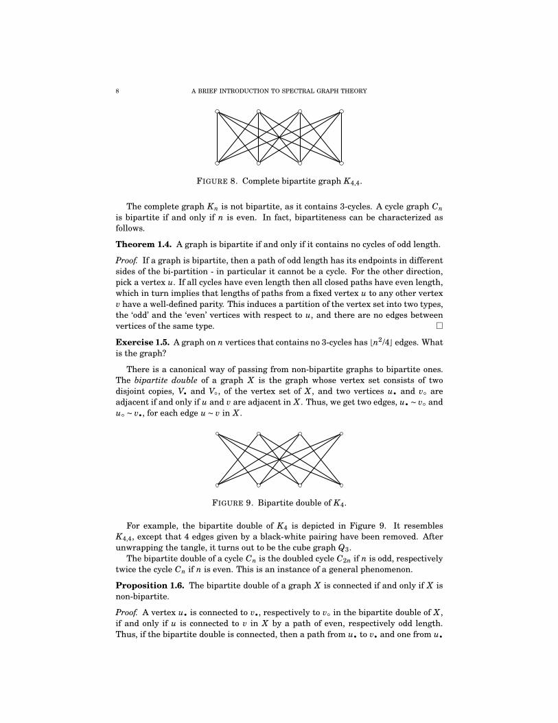
FIGURE 8. Complete bipartite graph K4,4.
The complete graph Kn is not bipartite, as it contains 3-cycles. A cycle graph Cn
is bipartite if and only if n is even. In fact, bipartiteness can be characterized asfollows.
Theorem 1.4. A graph is bipartite if and only if it contains no cycles of odd length.
Proof. If a graph is bipartite, then a path of odd length has its endpoints in differentsides of the bi-partition - in particular it cannot be a cycle. For the other direction,pick a vertex u. If all cycles have even length then all closed paths have even length,which in turn implies that lengths of paths from a fixed vertex u to any other vertexv have a well-defined parity. This induces a partition of the vertex set into two types,the ‘odd’ and the ‘even’ vertices with respect to u, and there are no edges betweenvertices of the same type. �
Exercise 1.5. A graph on n vertices that contains no 3-cycles has ⌊n2/4⌋ edges. Whatis the graph?
There is a canonical way of passing from non-bipartite graphs to bipartite ones.The bipartite double of a graph X is the graph whose vertex set consists of twodisjoint copies, V• and V◦, of the vertex set of X , and two vertices u• and v◦ areadjacent if and only if u and v are adjacent in X . Thus, we get two edges, u• ∼ v◦ andu◦ ∼ v•, for each edge u∼ v in X .
FIGURE 9. Bipartite double of K4.
For example, the bipartite double of K4 is depicted in Figure 9. It resemblesK4,4, except that 4 edges given by a black-white pairing have been removed. Afterunwrapping the tangle, it turns out to be the cube graph Q3.
The bipartite double of a cycle Cn is the doubled cycle C2n if n is odd, respectivelytwice the cycle Cn if n is even. This is an instance of a general phenomenon.
Proposition 1.6. The bipartite double of a graph X is connected if and only if X isnon-bipartite.
Proof. A vertex u• is connected to v•, respectively to v◦ in the bipartite double of X ,if and only if u is connected to v in X by a path of even, respectively odd length.Thus, if the bipartite double is connected, then a path from u• to v• and one from u•

A BRIEF INTRODUCTION TO SPECTRAL GRAPH THEORY 9
to v◦ yield a close path of odd length in X , so X is non-bipartite. Conversely, assumethat X is non-bipartite, so X contains some cycle of odd length. Pick a vertex u onthe cycle. We claim that, in X , we can join u to any other vertex v by a path of evenlength, as well as by one of odd length. Indeed, take a path p from u to v. Then pand the path p′, obtained by first going once around the cycle and then following p,are two paths from u to v of different parities. In the bipartite double, this meansthat u• is connected to v• and to v◦, no matter what v is. Thus, the bipartite doubleis connected. �
The upshot is that we will only take bipartite doubles of non-bipartite graphs.But we can also ask the reverse question: given a bipartite graph, is it the bipar-
tite double of some other graph? A first exercise in this direction, left to the reader,is that a tree is not a bipartite double.
2. INVARIANTS
A graph invariant is some property of a graph, most commonly a number, that ispreserved by isomorphisms. There is a great variety of numerical invariants that onecan associate to a graph, besides the fundamental parameters n (the size) and d (themaximal degree). Among the most important, and the ones we are interested herein,are the chromatic number, the independence number, the diameter, the girth, andthe isoperimetric constant. Roughly speaking, the first two measure the freeness,the next two the largeness, and the last one the connectivity of a graph.
Chromatic number and independence number.
The chromatic number, denoted χ, is the minimal number of colours needed topaint the vertices in such a way that adjacent vertices have different colours. Theindependence number, denoted ι, is the maximal number of vertices that can be cho-sen so that no two of them are adjacent. A set of vertices is said to be independent ifno two vertices are adjacent.
The chromatic number satisfies 2 ≤ χ ≤ n. At the extremes, χ = 2 characterizesbipartite graphs whereas χ = n characterizes the complete graph Kn. The indepen-dence number satisfies 1≤ ι≤ n−1. The lowest value ι= 1 characterizes the completegraph Kn, while the highest value ι= n−1 characterizes the star graph on n vertices.
Kn Cn Qn Kn,n Petersen
chromatic χ n 2 or 3 2 2 3
independence ι 1 ⌊n/2⌋ 2n−1 n 4
The chromatic number and the independence number are related by the followingfact.
Proposition 2.1. We have χ · ι≥ n.
Proof. Consider a colouring with χ colours. Then the vertex set is partitioned intoχ monochromatic sets. Furthermore, each monochromatic set of vertices is indepen-dent so its size is at most ι. �

10 A BRIEF INTRODUCTION TO SPECTRAL GRAPH THEORY
The obvious bound χ≤ n can be improved as follows.
Proposition 2.2. We have χ≤ d+1.
Proof. We argue by induction on n. Consider the (possibly disconnected) graph ob-tained after deleting some vertex. It can be coloured by using d + 1 colours. Thedeleted vertex has at most d neighbours, so at least one more colour is available tocomplete the colouring. �
The previous proposition is sharp: complete graphs and odd cycles satisfy χ= d+1.Nevertheless, it can be strengthened as follows.
Theorem 2.3 (Brooks). We have χ≤ d except for complete graphs and odd cycles.
Exercise 2.4. Show that χ≤ d for irregular graphs.
Notes. The chromatic number is the oldest graph invariant. Much of the early workin graph theory was motivated by a cartographic observation that we now call theFour-Colour Theorem.
Theorem 2.3 is due to Brooks (On colouring the nodes of a network, Proc. Cam-bridge Philos. Soc. 1941). The original proof, but also the modern approaches, aresomewhat involved. Exercise 2.4 covers the easy case when the graph is not regular.
Diameter and girth.
The diameter, denoted δ, is the maximal distance between vertices. The girth,denoted γ, is the minimal length of a cycle.
The diameter satisfies 1 ≤ δ ≤ n− 1. At the extremes, δ = 1 characterizes thecomplete graph Kn, and δ = n− 1 characterizes the path on n vertices. The girthsatisfies 3 ≤ γ≤ n, unless we are dealing with a tree in which case we put γ=∞. Thevalue γ= n characterizes the cycle Cn.
Kn Cn Qn Kn,n Petersen
diameter δ 1 ⌊n/2⌋ n 2 2
girth γ 3 n 4 4 5
For graphs which are not trees, the diameter and the girth are related as follows.
Proposition 2.5. We have γ≤ 2δ+1. If γ is even, then actually γ≤ 2δ.
Proof. We have to show that δ ≥ ⌊γ/2⌋. Assume that, on the contrary, δ < ⌊γ/2⌋.Consider a cycle of length γ in the graph, and pick two vertices u and v at distance⌊γ/2⌋ as measured along the cycle. On the other hand, u and v can be connected bya path of length at most δ. So we have two paths from u to v whose lengths areequal to ⌊γ/2⌋, respectively less than ⌊γ/2⌋. In particular, the two paths are distinct.It follows that there is a cycle whose length is less than 2⌊γ/2⌋. As 2⌊γ/2⌋ ≤ γ, this isa contradiction. �
The next result gives bounds for diameter and the girth in terms of the funda-mental parameters.
A BRIEF INTRODUCTION TO SPECTRAL GRAPH THEORY 11
Theorem 2.6. Assume d ≥ 3. Then we have
δ>logn
log(d−1)−2.
For a regular graph, we also have
γ< 2logn
log(d−1)+2.
Proof. Let u be a fixed vertex. Then balls around u grow at most exponentially withrespect to the radius:
|Br(u)| ≤ 1+d+d(d−1)+ . . .+d(d−1)r−1 < d(d−1)r
If r = δ then the ball Br(u) is the entire vertex set, so n < d(d − 1)δ. Thereforeδ> logd−1 n− logd−1 d. As logd−1 d < 2, we get the claimed lower bound on δ.
Let us turn to the girth bound for regular graphs. Note, incidentally, that thegirth is well-defined: a regular graph cannot be a tree. We exploit the idea that,for a certain short range, balls around u achieve exponential growth in the radius.Namely, as long as 2r < γ we have
|Br(u)| = 1+d+d(d−1)+ . . .+d(d−1)r−1 > (d−1)r.
Take r largest possible subject to 2r < γ. Then γ≤ 2r+2 while n ≥ |Br(u)| > (d−1)r ,in other words r < logd−1 n. The claimed upper bound for the girth follows. �
The bounds of the previous theorem become particularly appealing when viewedin an asymptotic light. A d-regular family is an infinite sequence of d-regular graphs{Xk} with |Xk| →∞. For a d-regular family with d ≥ 3, Theorem 2.6 says that thediameter growth is at least logarithmic in the size, δk ≫ log |Xk|, while the girthgrowth is at most logarithmic in the size, γk ≪ log |Xk |. Here, we are using thefollowing growth relation on sequences: ak ≪ bk if there is a constant C such thatak ≤ Cbk for all k.
At this point, it is natural to ask about extremal families. A d-regular family {Xk}is said to have small diameter if δk ≍ log |Xk |, respectively large girth if γk ≍ log |Xk |.The growth equivalence of sequences is defined as follows: ak ≍ bk if and only ifak ≪ bk and ak ≫ bk.
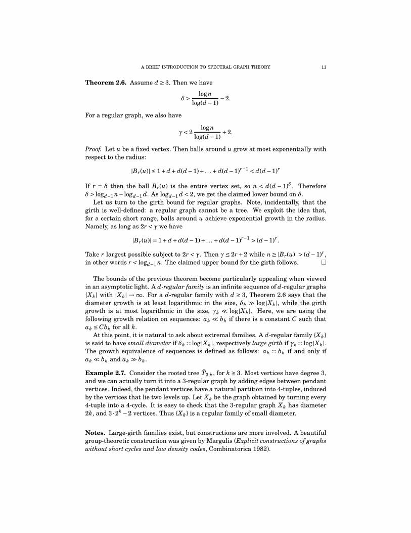
Example 2.7. Consider the rooted tree T3,k, for k ≥ 3. Most vertices have degree 3,and we can actually turn it into a 3-regular graph by adding edges between pendantvertices. Indeed, the pendant vertices have a natural partition into 4-tuples, inducedby the vertices that lie two levels up. Let Xk be the graph obtained by turning every4-tuple into a 4-cycle. It is easy to check that the 3-regular graph Xk has diameter2k, and 3 ·2k −2 vertices. Thus {Xk} is a regular family of small diameter.
Notes. Large-girth families exist, but constructions are more involved. A beautifulgroup-theoretic construction was given by Margulis (Explicit constructions of graphswithout short cycles and low density codes, Combinatorica 1982).

12 A BRIEF INTRODUCTION TO SPECTRAL GRAPH THEORY
FIGURE 10. The graph X3.
Isoperimetric number.
For a non-empty vertex subset S in a graph, the boundary ∂S is the set of edgesconnecting S to its complement Sc . Note that S and Sc have the same boundary.
The isoperimetric constant, denoted β, is given by
β=minS
|∂S||S|
where the minimum is taken over all vertex subsets S that contain no more thanhalf the vertices. A set S on which β is attained is said to be an isoperimetric set.
Finding β can be quite difficult, even on small or familiar graphs. Unlike allthe previous graph invariants, which are integral, the isoperimetric constant β isrational. It is therefore harder to limit possibilities in a trial-and-error approach. Inconcrete examples, it can be quite easy to give an upper bound for β, by means of awell-chosen vertex subset. However, proving a matching lower bound for β is usuallymuch harder.
Example 2.8. Consider the cube graph Qn. The binary strings starting in 0 definea subset S containing half the number of vertices of Qn, and |∂S|/|S| = 1 since everyvertex in S has one external edge. Thus β≤ 1. We claim that, in fact, β= 1.
We think of Qn as the product K2 ×·· ·×K2. We wish to argue that β(X ×K2) = 1whenever β(X ) = 1. As β(K2) = 1, the bound β(X × K2) ≤ 1 is an instance of thegeneral principle that
β(X ×Y ) ≤min{β(X ),β(Y )}.
Indeed, let S be an isoperimetric subset in X . In X ×Y , the boundary of the subsetS×Y is in bijection with (∂S)×Y . It follows that β(X ×Y ) ≤ β(X ), and similarly forβ(Y ).
The trickier bit is to show that β(X ×K2)≥ 1. We visualize X ×K2 as two ‘horizon-tal’ copies of X , X• and X◦, with additional ‘vertical’ edges joining v• to v◦ for eachvertex v in X . A vertex subset S in X ×K2 is of the form A•∪B◦, where A and B arevertex subsets in X . The boundary of S in X ×K2 has horizontal edges, correspond-ing to the boundary of A, respectively B, in X , and vertical edges, corresponding tothe symmetric difference A△B. Thus, |∂S| = |∂A| + |∂B| + |A△B|. We have to showthat
|∂A|+ |∂B|+ |A△B| ≥ |A|+ |B|

A BRIEF INTRODUCTION TO SPECTRAL GRAPH THEORY 13
whenever |A| + |B| ≤ |X |. If |A|, |B| ≤ |X |/2, then we already have |∂A| ≥ |A| and|∂B| ≥ |B|. If |A| ≥ |X |/2 ≥ |B|, then |∂B| ≥ |B|, |∂A| ≥ |Ac | = |X |−|A| ≥ |B|, and |A△B| ≥|A|− |B|. Adding up these inequalities completes the argument.
Exercise 2.9. Show that β(Kn)= ⌈n/2⌉; β(Cn)= 2/⌊n/2⌋; β(Kn,n) = ⌈n2/2⌉/n; β= 1 forthe Petersen graph.
Kn Cn Qn Kn,n Petersen
isoperimetric β ∼ n/2 ∼ 4/n 1 ∼ n/2 1
This table records our findings in asymptotic form: we write an ∼ bn if an/bn → 1as n→∞.
The isoperimetric constant clearly satisfies 0< β≤ d. Taking a subset S consistingof two adjacent vertices, the upper bound can be improved to d−1. But a more carefulargument, explained below, yields an upper bound of roughly d/2. Note, however,that β may slightly exceed d/2. This is the case for Kn and Kn,n, for odd n.
Theorem 2.10. We have:
β≤d
2·
n+1
n−1
Proof. For 1 ≤ s ≤ ⌊n/2⌋, we let βs denote the minimum of |∂S|/|S| as S runs oververtex subsets of size s. An upper bound for βs is the average
1
#{S : |S| = s}
∑
|S|=s
|∂S||S|
which we can actually compute. Any given edge is in the boundary of 2(
n−2s−1
)
sub-sets of size s, so the numerator is
∑
|S|=s |∂S| = 2|E|(
n−2s−1
)
. The denominator is s( n
s)
.Simplifying, we deduce that
βs ≤2|E|(n− s)
n(n−1).
As 2|E| ≤ dn, we get
β=mins
βs ≤ mins
d(n− s)
n−1=
d(n−⌊n/2⌋)n−1
which is actually slightly better than the claim. �
Exercise 2.11. Let Br(u) denote the ball of radius r around a vertex u. Prove thefollowing short-range exponential growth behaviour: |Br(u)| ≥ (1+β/d)r as long as|Br−1(u)| ≤ n/2. Conclude that
δ≤2log(n/2)
log(1+β/d)+2.
Let us explain an important qualitative consequence of this exercise. A d-regularfamily {Xk} is said to be an expander if the sequence of isoperimetric constants {βk} isbounded away from 0. This is a very interesting condition: roughly speaking, an ex-pander family is an infinite sequence of sparse graphs which nevertheless maintaina sizable connectivity. Exercise 2.11 implies the following fact: an expander familyhas small diameter. Note that the converse does not hold. The small-diameter family{Xk} of Example 2.7 is not an expander. Indeed, if S is the set of vertices lying on one

14 A BRIEF INTRODUCTION TO SPECTRAL GRAPH THEORY
of the three main branches stemming from the root, then |∂S| = 1 and |S| = 2k −1.Thus βk → 0 exponentially fast.
Notes. Among the five invariants under consideration, the isoperimetric constantis the youngest. To the best of our knowledge, it was introduced by Buser (Cubicgraphs and the first eigenvalue of a Riemann surface, Math. Z. 1978). This partlyexplains our choice of notation, β. Elsewhere, the isoperimetric constant is denotedby h or i, and it is also called the Cheeger constant because it is the graph-theoreticanalogue of an isoperimetric constant for manifolds, denoted h, due to Cheeger (Alower bound for the smallest eigenvalue of the Laplacian, in ‘Problems in analysis’,Princeton University Press 1970). Other sources call it conductance, and denote itby φ or Φ.
Theorem 2.10 is due to Mohar (Isoperimetric numbers of graphs, J. Combin. The-ory Ser. B 1989).
3. REGULAR GRAPHS I
In this section, we focus on constructions of regular graphs from groups. Themost important notion here is that of a Cayley graph. We also discuss a bipartitevariation, that of a bi-Cayley graph.
Cayley graphs.
Let G be a finite group. Let S ⊆ G be a subset that does not contain the identityof G, and which is symmetric (i.e., closed under taking inverses) and generating (i.e.,every element of G is a product of elements of S). The Cayley graph of G with respectto S has the elements of G as vertices, and an edge between every two verticesg,h ∈ G satisfying g−1h ∈ S. In other words, the neighbours of a vertex g are thevertices of the form gs, where s ∈ S.
The Cayley graph of G with respect to S an |S|-regular graph of size |G|. Theassumptions on G and S reflect our standing convention that graphs should be finite,connected, and simple.
Example 3.1. The Cayley graph of a group G with respect to the set of non-identityelements of G is the complete graph on n= |G| vertices.
Example 3.2. The Cayley graph of Zn with respect to {±1} is the cycle graph Cn.
Example 3.3. The Cayley graph of (Z2)n with respect to {e i = (0, . . . ,0,1,0, . . . ,0) : i =1, . . . ,n} is the cube graph Qn.
Example 3.4. The halved cube graph 12Qn is defined as follows: its vertices are
those binary strings of length n that have an even weight, and edges connect twosuch strings when they differ in precisely two slots. This is the Cayley graph of thesubgroup
{
v ∈ (Z2)n :∑
vi = 0}
with respect to {e i + e j : 1≤ i < j ≤ n}.
Example 3.5. (The twins) Here we consider two Cayley graphs coming from thesame group, Z4 ×Z4. The two symmetric generating sets are as follows:
S1 = {±(1,0),±(0,1),(2,0),(0,2)}
S2 = {±(1,0),±(0,1),±(1,1)}

A BRIEF INTRODUCTION TO SPECTRAL GRAPH THEORY 15
The corresponding Cayley graphs are 6-regular graphs on 16 vertices. It is not hardto recognize the Cayley graph with respect to S1 as the product K4×K4. The secondCayley graph, with respect to S2, is known as the Shrikhande graph. Both aredepicted in Figure 11. An amusing puzzle, left to the reader, is to check the picturesby finding an appropriate Z4 ×Z4 labeling. The more interesting one is, of course,the Shrikhande graph.
FIGURE 11. K4 ×K4 and the Shrikhande graph.
It seems quite appropriate to think of these two graphs as being twins. Not onlyare they Cayley graphs of the same group, but they also turn out to be indistinguish-able by any of the five invariants under consideration! Both graphs have diameter 2and girth 3. They also have the same chromatic number, χ= 4. Indeed, we get a nice4-colouring for both graphs by noting that the addition homomorphism Z4×Z4 →Z4,given by (a,b) 7→ a+ b, is non-trivial on both sets of generators. On the other hand,three colours are not sufficient for K4 ×K4, as it contains K4 as a subgraph; in theShrikhande graph, it is the outer octagon that cannot be 3-coloured. Next, bothgraphs have independence number ι = 4. Firstly, we know that ι ≥ 4 by using theinequality χ× ι≥ 16. Secondly, we easily find independent sets of size 4 in each oneof the two graphs. Finally, both graphs turn out to have isoperimetric constant 2. Aconceptual explanation for this fact will be given later on, using spectral ideas.
Example 3.6. Let n ≥ 3. The Cayley graph of Z3n−1 with respect to the symmetricgenerating set S = {1,4, . . . ,3n−2} is known as the Andrásfai graph An.
Exercise 3.7. Show that the Andrásfai graph An has diameter 2, girth 4, chromaticnumber 3, and independence number n.
Example 3.8. Let us view the five Platonic solids as graphs. The tetrahedron andthe cube yield two familiar graphs, K4 and Q3. The next three are the octahedralgraph (Figure 12), the icosahedral graph (Figure 13), and the dodecahedral graph(Figure 14).
The octahedral graph can be realized as the Cayley graph of Z6 with respect to{±1,±2}. Another realization is on the dihedral group with 6 elements. We think ofthis group as the semidirect product Z3⋊ {±1}: the underlying set is Z3 × {±1}, withoperation (a,ǫ)(b,τ) = (a+ ǫb,ǫτ). The elements in Z3 × {−1} are involutions, and theremaining two non-trivial elements, (±1,1), are inverse to each other. A symmetric

16 A BRIEF INTRODUCTION TO SPECTRAL GRAPH THEORY
FIGURE 12. Two views of the octahedral graph.
FIGURE 13. Two views of the icosahedral graph.
FIGURE 14. Two views of the dodecahedral graph.
subset S of size 4 must contain these two elements, and two more involutions pickedfrom Z3×{−1}. The Cayley graph with respect to any one of the three possible choicesfor S is the octahedral graph. There is a good reason why this is the case: there isjust one 4-regular graph on 6 vertices.
The icosahedral graph is a Cayley graph, as well. Namely, it is the Cayley graph ofthe alternating group Alt(4) with respect to the set {(123),(132),(234),(243),(12)(34)}.
Example 3.9. As we know, a cube graph is bipartite. Is a cube graph a bipartitedouble?
We start from Qn+1, and we look for an (n+1)-regular graph on 2n vertices. Addingone edge per vertex to Qn would be such a graph. So let us consider the Cayley graphof (Z2)n with respect to {e1, . . . , en,a}, where the new generator a ∈ (Z2)n has weightgreater than 1. This Cayley graph is referred to as the decked cube graph DQn(a) inwhat follows.

A BRIEF INTRODUCTION TO SPECTRAL GRAPH THEORY 17
A decked cube graph only depends on the weight of the new generator. Indeed, leta and a′ have equal weight. Then we can actually set up a Cayley graph isomorphismbetween DQn(a) and DQn(a′), that is, a group isomorphism between the underlyinggroups which maps one generating set onto the other. For there is a permutation ofthe basis {e1, . . . , en} which, once extended to a group automorphism of (Z2)n, maps ato a′.
A decked cube graph is bipartite if and only if the new generator has odd weight.To see this, consider the bipartition of Qn according to weight parity. Then the newedges join vertices of different colour precisely when the weight of the new generatoris odd.
So we focus on a decked cube graph DQn(a) where a ∈ (Z2)n has even weight,and we claim that its bipartite double is Qn+1. Note the following general fact: thebipartite double of the Cayley graph of a group G with respect to S is the Cayleygraph of G ×Z2 with respect to S × {1}. So the bipartite double of DQn(a) is theCayley graph of (Z2)n+1 with respect to {(e1,1), . . . ,(en,1),(a,1)}. To show that thelatter graph is Qn+1, we use again a Cayley graph isomorphism. We adopt a linearalgebra perspective, viewing Z2 as field. Let A be the (n+1)-by-(n+1) matrix over Z2
with rows (e1,1), . . . ,(en,1),(a,1). Then v 7→ Av defines a group homomorphism from(Z2)n+1 to itself, mapping the standard basis e′1, . . . , e′n+1 to (e1,1), . . . ,(en,1),(a,1). Weare left with checking that the matrix A is invertible, equivalently, that the binarystrings (e1,1), . . . ,(en,1),(a,1) are linearly independent in (Z2)n+1. Let
c0(a,1)+n∑
i=1ci(e i ,1)= 0
for some coefficients ci ∈ Z2. Then c0 = c1 + . . .+ cn and c0a = (c1, . . . , cn). If c0 = 1then a has odd weight, contradicting our assumption on a. Hence c0 = 0, and c1 =. . . = cn = 0 follows as well.
Returning to our starting question, we infer that Qn+1 is a bipartite double assoon as there is an element of (Z2)n having even, but non-zero weight. This holds forn≥ 2, so all cube graphs starting from Q3 are bipartite doubles. As for Q2, it is not abipartite double.
Notes. Cayley graphs were introduced by Cayley in 1878.
Vertex-transitive graphs.
A graph is said to be vertex-transitive if any vertex can be taken to any othervertex by a graph automorphism.
Proposition 3.10. Cayley graphs are vertex-transitive.
Proof. Consider a Cayley graph of a group G. We look for a graph automorphismtaking the identity vertex to an arbitrary vertex g ∈ G. Left multiplication by g,namely the mapping h 7→ gh, does the job. �
Exercise 3.11. Consider the Cayley graph of a group G with respect to S. Showthat the following are equivalent: (i) for each g ∈ G, right multiplication by g is agraph automorphism; (ii) inversion on G, g 7→ g−1, is a graph automorphism; (iii) Sis closed under conjugation.

18 A BRIEF INTRODUCTION TO SPECTRAL GRAPH THEORY
Example 3.12. The Petersen graph is vertex-transitive. Let us give two arguments,according to how we choose to think of the Petersen graph.
Symbolically, the Petersen graph records the relation of disjointness between 2-element subsets of a 5-element set S. A permutation of S maps 2-element subsetsto 2-element subsets, and it does so in a disjointness-preserving fashion. So any per-mutation of S defines an automorphism of the Petersen graph. To conclude, observethat any 2-element subset of S can be taken to any other one by a permutation.
Graphically, we think of the Petersen graph in its pentagram-within-pentagondrawing. Consider a labeling of the vertices as in the right-most panel of the trip-tych in Figure 15. Note that there is an obvious 5-fold rotational symmetry. So thevertices of the outer pentagon, 1 through 5, are in the same orbit of the automor-phism group, and the same is true for the vertices of the outer pentagon, a throughe. We need an automorphism that mixes up the two orbits. This is explained in thenext two panels of Figure 15: switch b and 3, respectively e and 4, and then switchc and d. A mixing automorphism can be read off by comparing the first and the lastpanels.
1
2 5
3 4
a
b e
c d
1
2 5
b e
a
3 4
c d
1
2 5
b e
a
3 4
d c
FIGURE 15
Example 3.13. The five Platonic graphs are vertex-transitive. Reflections take anyface to any other face. Within each face, we can get from any vertex to any othervertex by using rotations. Recall that all but one of them, the dodecahedral graph,are in fact Cayley graphs.
Example 3.14. Are there vertex-transitive graphs which are not Cayley graphs?The answer is positive, as one might guess, but providing examples is not such aneasy matter. Let us show that the Petersen graph and the dodecahedral graph, bothof which we already know to be vertex-transitive, are not Cayley graphs.
The Petersen graph and the dodecahedral graph have two noticeable features incommon: both are 3-regular, and have girth 5. Consider a Cayley graph havingthese two properties. Then there are two cases, according to whether the symmetricgenerating set S contains one or three involutions.
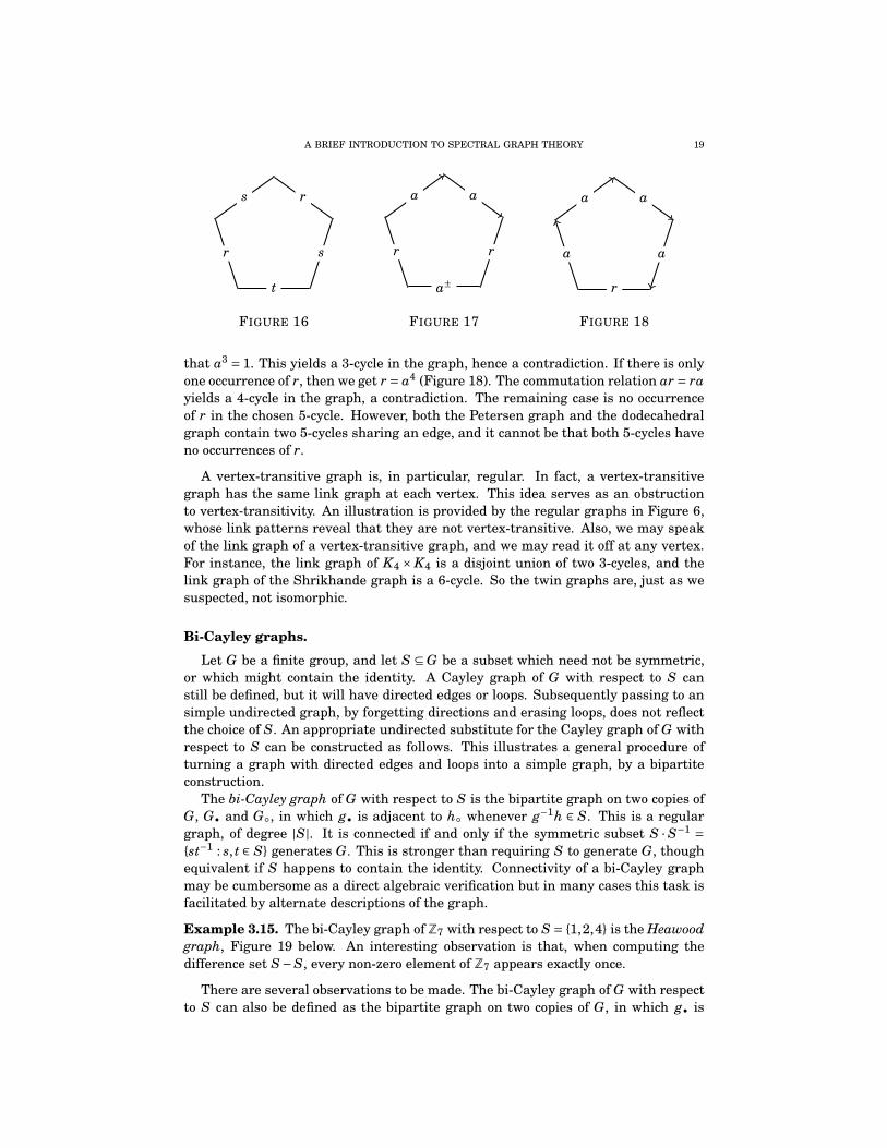
Let S = {r,s, t}, where r2 = s2 = t2 = 1. The edges of a 5-cycle are labeled by r, s, ort. Two consecutive edges have different labels, so one of labels, say t, appears onlyonce. Up to swapping r and s, we may assume that we have the labeling of Figure 16.Then t= (rs)2 = (sr)2. It follows that r commutes with t: rt= r(sr)2 = (rs)2r = tr. Thismeans that there is a 4-cycle in the graph, a contradiction.
Let S = {r,a,a−1 }, where r2 = 1. Label again the edges of a 5-cycle by the genera-tors. There can be at most two occurrences of r. If there are two occurrences, then weget the relation rar = a±2 (Figure 17). But then a = ra±2r = (rar)±2 = a4, meaning
A BRIEF INTRODUCTION TO SPECTRAL GRAPH THEORY 19
s r
sr
t
FIGURE 16
a a
rr
a±
FIGURE 17
a a
aa
r
FIGURE 18
that a3 = 1. This yields a 3-cycle in the graph, hence a contradiction. If there is onlyone occurrence of r, then we get r = a4 (Figure 18). The commutation relation ar = rayields a 4-cycle in the graph, a contradiction. The remaining case is no occurrenceof r in the chosen 5-cycle. However, both the Petersen graph and the dodecahedralgraph contain two 5-cycles sharing an edge, and it cannot be that both 5-cycles haveno occurrences of r.
A vertex-transitive graph is, in particular, regular. In fact, a vertex-transitivegraph has the same link graph at each vertex. This idea serves as an obstructionto vertex-transitivity. An illustration is provided by the regular graphs in Figure 6,whose link patterns reveal that they are not vertex-transitive. Also, we may speakof the link graph of a vertex-transitive graph, and we may read it off at any vertex.For instance, the link graph of K4 ×K4 is a disjoint union of two 3-cycles, and thelink graph of the Shrikhande graph is a 6-cycle. So the twin graphs are, just as wesuspected, not isomorphic.
Bi-Cayley graphs.
Let G be a finite group, and let S ⊆ G be a subset which need not be symmetric,or which might contain the identity. A Cayley graph of G with respect to S canstill be defined, but it will have directed edges or loops. Subsequently passing to ansimple undirected graph, by forgetting directions and erasing loops, does not reflectthe choice of S. An appropriate undirected substitute for the Cayley graph of G withrespect to S can be constructed as follows. This illustrates a general procedure ofturning a graph with directed edges and loops into a simple graph, by a bipartiteconstruction.
The bi-Cayley graph of G with respect to S is the bipartite graph on two copies ofG, G• and G◦, in which g• is adjacent to h◦ whenever g−1h ∈ S. This is a regulargraph, of degree |S|. It is connected if and only if the symmetric subset S ·S−1 ={st−1 : s, t ∈ S} generates G. This is stronger than requiring S to generate G, thoughequivalent if S happens to contain the identity. Connectivity of a bi-Cayley graphmay be cumbersome as a direct algebraic verification but in many cases this task isfacilitated by alternate descriptions of the graph.
Example 3.15. The bi-Cayley graph of Z7 with respect to S = {1,2,4} is the Heawoodgraph, Figure 19 below. An interesting observation is that, when computing thedifference set S−S, every non-zero element of Z7 appears exactly once.
There are several observations to be made. The bi-Cayley graph of G with respectto S can also be defined as the bipartite graph on two copies of G, in which g• is

20 A BRIEF INTRODUCTION TO SPECTRAL GRAPH THEORY
FIGURE 19. The Heawood graph.
adjacent to h◦ whenever gh ∈ S. This adjacency law is more symmetric, and tends toappear more often in practice. The correspondence g• ↔ (g−1)•, h◦ ↔ h◦ shows theequivalence of the two descriptions.
If S is such that the Cayley graph of G with respect to S already makes sense,then its bipartite double is the bi-Cayley graph of G with respect to S. We interpretthis as saying that the bi-Cayley graph construction is essentially a generalizationof the Cayley graph construction.
The bi-Cayley graph of G with respect to S is a Cayley graph in many cases ofinterest. Namely, assume G is an abelian group, and consider the semidirect productG⋊{±1} given by inversion. This means that we endow the set G×{±1} with the non-abelian operation (g,ǫ)(h,τ) = (ghǫ ,ǫτ) for g,h ∈ G and ǫ,τ ∈ {±1}. If G happens to bea cyclic group, then G ⋊ {±1} is a dihedral group. This familiar instance promptsus to deem G⋊ {±1} a generalized dihedral group. The advantage of the semidirectproduct over the direct product G×{±1} is that now S×{−1} is symmetric in G⋊{±1},for it consists of involutions. The Cayley graph of G⋊ {±1} with respect to S× {−1} isa bipartite graph on G×{+1} and G×{−1}, with (g,+1) connected to (h,−1) wheneverg−1h ∈ S. This is precisely the bi-Cayley graph of G with respect to S.
4. REGULAR GRAPHS II
This section introduces some types of regular graphs. Their common feature isthat the number of neighbours shared by pairs of vertices is severely restricted.
Strongly regular graphs.
A regular graph is said to be strongly regular if there are two non-negative inte-gers a and c such that any two adjacent vertices have a common neighbours, andany two distinct non-adjacent vertices have c common neighbours.
Example 4.1. The Petersen graph is strongly regular, with a= 0 and c= 1.
Example 4.2. The cycle C5 is strongly regular, with a= 0 and c = 1. The only othercycle which is strongly regular is C4, which has a= 0 and c= 2.
Example 4.3. The complete bipartite graph Kn,n is strongly regular, with a= 0 andc= n. No other bipartite graph is strongly regular.

A BRIEF INTRODUCTION TO SPECTRAL GRAPH THEORY 21
Example 4.4. The rook’s graph Kn×Kn is strongly regular, with a= n−2 and c= 2.No other non-trivial product is strongly regular.
Example 4.5. The twin graphs, K4 × K4 and the Shrikhande graph, are stronglyregular with a= c= 2.
The complete graph Kn has a = n−2 but undefined c. Treating it as a stronglyregular graph is a matter of convention, and ours is to exclude it.
The parameters (n,d,a, c) of a strongly regular graph are constrained by a numberof relations. The simplest one is the following:
Proposition 4.6. The parameters (n,d,a, c) of a strongly regular graph satisfy
d(d−a−1) = (n−d−1)c.
Proof. Fix a base vertex; its link graph has d vertices, and there are n−d−1 farthervertices. The desired relation comes from counting in two ways the edges betweenlink vertices and farther vertices.
Each link vertex has a common neighbours with the base vertex. In other words,the link graph is a-regular. So each link vertex is adjacent to d−a−1 farther vertices.
Each farther vertex has c common neighbours with the base vertex. That is, eachfarther vertex is adjacent to c link vertices. �
As we have seen, the link graph of any vertex is an a-regular graph on d vertices.It cannot be complete on d vertices - if it were, the whole graph would be completeon d+1 vertices. So a< d−1, and c> 0. The latter fact means the following.
Proposition 4.7. A strongly regular graph has diameter 2.
There are non-isomorphic strongly regular graphs with the same parameters(n,d,a, c). For example, the twin graphs have parameters (16,6,2,2). The follow-ing construction provides many more examples of this kind.
Theorem 4.8. Fix a positive integer n. Let G be a finite group with n elements, andlet XG be the Cayley graph of G×G with respect to the symmetric generating subset{(s,1),(1,s),(s, s) : s ∈G,s 6= 1}. Then:
(i) XG is strongly regular with parameters (n2,3n−3,n,6),(ii) the number of elements of order 2 in G is a graph invariant of XG .
Proof. Part (i) is straightforward counting. Pick two vertices in XG , one of whichmay be assumed to be the identity (1,1). Its neighbors are of the form (s,s), or (s,1),or (1,s) with s 6= 1. There are n common neighbours in each case: (s,1), (1,s), and(t, t) with t 6= 1,s; (s,s), (1,s), and (t,1) with t 6= 1,s; (s,s), (s,1), and (1, t) with t 6= 1,s.Now take a vertex (x, y) not adjacent to (1,1), meaning that x 6= 1, y 6= 1, and x 6= y.Then (x, y) has 6 common neighbours with (1,1), namely (x,x) and (y, y), (x,1) and(xy−1,1), (1, y) and (1, yx−1).
(ii) Consider the link graph of XG . It has 3n−3 vertices, and it is n-regular. Thevertices of the link at (1,1) are naturally partitioned into three ‘islands’: S1 = {(s,1) :s 6= 1}, S2 = {(1,s) : s 6= 1}, and S3 = {(s,s) : s 6= 1}. Each Si is a complete subgraph onn−1 vertices. A vertex has n−2 incident edges within its own island, and two more‘bridge’ edges connecting it to the remaining two islands. It follows that 3-cycles inthe link graph are either contained in an island, or they consist of three vertices fromeach of the islands, connected by bridge edges. The number of 3-cycles contained inan island is a function of n. The number of 3-cycles of bridge type equals the number

22 A BRIEF INTRODUCTION TO SPECTRAL GRAPH THEORY
of elements of order 2 in G. Indeed, the paths of length 3 starting and ending in S2,say, along bridge edges have the form (s,1) ∼ (s,s) ∼ (1,s) ∼ (s−1,1). This is a 3-cycleprecisely when s has order 2. In conclusion, the number of elements of order 2 in Gis a graph invariant of the link graph of XG , hence of XG itself, when the order of Gis fixed. �
Corollary 4.9. For every positive integer N, there exist N strongly regular graphsthat are pairwise non-isomorphic, but have the same parameters.
Proof. For k = 1, . . . ,N, consider the abelian group G(k) = (Z2)k−1×Z2N−k . Then G(k)has size 2N−1, and 2k−1 elements of order 2. The previous theorem implies that thegraphs XG(k), k = 1, . . . ,N, are strongly regular with the same parameters, but theyare mutually non-isomorphic. �
Notes. Strongly regular graphs were introduced by Bose (Strongly regular graphs,partial geometries and partially balanced designs, Pacific J. Math. 1963). TheShrikhande graph was originally defined by Shrikhande (The Uniqueness of the L2
Association Scheme, Ann. Math. Stat. 1959) in a combinatorial way that madestrong regularity immediate.
Design graphs.
Next, we consider bipartite analogues of strongly regular graphs.A design graph is a regular bipartite graph with the property that any two dis-
tinct vertices of the same colour have the same number of common neighbours. Thecomplete bipartite graph Kn,n fits the definition, but we exclude it by convention.
For a design graph, we let m denote the half-size, d the degree, and c the numberof neighbours shared by any monochromatic pair of vertices. Note that the parame-ter c is, in fact, determined by the following relation:
c(m−1) = d(d−1)
This is obtained by counting in two ways the paths of length 2 joining a fixed vertexwith the remaining m−1 vertices of the same colour.
As an immediate consequence of the definition, we have following fact.
Proposition 4.10. A design graph has diameter 3, and girth 4 or 6 according towhether c > 1 or c = 1. Conversely, a regular bipartite graph of diameter 3 and girth6 is a design graph with parameter c= 1.
Design graphs with parameter c = 1 are particularly interesting. The previousproposition highlights them as being extremal for the girth among regular bipartitegraph of diameter 3. The next exercise is concerned with another extremal property.
Exercise 4.11. Design graphs with parameter c = 1 and degree d are the ones thatminimize the number of vertices among all d-regular graphs of girth 6.
It seems appropriate to refer to design graphs with parameter c = 1 as extremaldesign graphs. There are some examples of extremal design graphs among thegraphs that we already know. One is the cycle C6. The other, more interesting,is the Heawood graph. In the next section, we will construct more design graphs,some of them extremal, by using finite fields.
A BRIEF INTRODUCTION TO SPECTRAL GRAPH THEORY 23
A partial design graph is a regular bipartite graph with the property that thereare only two possible values for the number of neighbours shared by any two distinctvertices of the same colour.
The parameters of a partial design graph are denoted m, d, respectively c1 andc2. Note that c1 6= c2, and that the roles of c1 and c2 are interchangeable.
Example 4.12. The bipartite double of a (non-bipartite) strongly regular graph is adesign graph or a partial design graph.
Example 4.13. The cube graph Qn is a partial design graph. Indeed, consider thebipartition given by weight parity. Fix two distinct strings with the same weightparity. If they differ in two slots, then they have two common neighbours; otherwise,they have no common neighbour. Thus, Qn has parameters of are c1 = 0, c2 = 2.
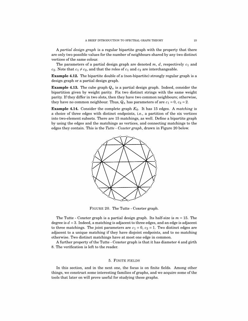
Example 4.14. Consider the complete graph K6. It has 15 edges. A matching isa choice of three edges with distinct endpoints, i.e., a partition of the six verticesinto two-element subsets. There are 15 matchings, as well. Define a bipartite graphby using the edges and the matchings as vertices, and connecting matchings to theedges they contain. This is the Tutte - Coxeter graph, drawn in Figure 20 below.
FIGURE 20. The Tutte - Coxeter graph.
The Tutte - Coxeter graph is a partial design graph. Its half-size is m = 15. Thedegree is d = 3. Indeed, a matching is adjacent to three edges, and an edge is adjacentto three matchings. The joint parameters are c1 = 0, c2 = 1. Two distinct edges areadjacent to a unique matching if they have disjoint endpoints, and to no matchingotherwise. Two distinct matchings have at most one edge in common.
A further property of the Tutte - Coxeter graph is that it has diameter 4 and girth8. The verification is left to the reader.
5. FINITE FIELDS
In this section, and in the next one, the focus is on finite fields. Among otherthings, we construct some interesting families of graphs, and we acquire some of thetools that later on will prove useful for studying these graphs.

24 A BRIEF INTRODUCTION TO SPECTRAL GRAPH THEORY
Notions.
Let us start by recalling some fundamental facts about finite fields.A finite field has q = pd elements for some prime p, the characteristic of the field,
and some positive integer d, the dimension of the field over its prime subfield.For each prime power q there exists a field with q elements, which is furthermore
unique up to isomorphism. We think of Zp =Z/pZ as ‘the’ field with p elements. Ingeneral, ‘the‘ field with q = pd elements can be realized as a quotient Zp[X ]/( f (X )),where f (X ) ∈ Zp[X ] is an irreducible polynomial of degree d. Such a polynomial fexists for each given d; however, no general recipe is known for producing one.
The multiplicative group of a finite field is cyclic. This is, again, a non-constructiveexistence: given a field, there is no known recipe for producing a multiplicative gen-erator.
We now turn to extensions of finite fields. The following result plays a key role inthis respect.
Theorem 5.1. Let K be a field with qn elements. Then the map φ : K→K, given byφ(a)= aq, has the following properties:
(i) φ is an automorphism of K of order n;(ii) F = {a ∈K : φ(a) = a} is a field with q elements, and φ is an F-linear isomor-
phism when K is viewed as a linear space over F.
Proof. (i) Clearly, φ is injective, multiplicative, and φ(1)= 1. To see that φ is additive,we iterate the basic identity (a+b)p = ap +bp, where p is the characteristic of K, upto (a+b)q = aq +bq. Thus φ is automorphism of K. Each a ∈K
∗ satisfies the relationaqn−1 = 1, so aqn = a for all a ∈K. Thus φn is the identity map on K. Assuming thatφt is the identity map on K for some 0 < t < n, we would get that X qt = X has qn
solutions in K, a contradiction.(ii) F is a subfield since φ is an automorphism. As K
∗ is cyclic of order qn −1, andq− 1 divides qn − 1, there are precisely q− 1 elements a ∈ K
∗ satisfying aq−1 = 1.Therefore F has q elements. Finally, note that φ(ab) = φ(a)φ(b) = aφ(b) whenevera ∈ F and b ∈K. �
Turning the above theorem on its head, we can start with a field F with q ele-ments, and then consider a field K with qn elements as an overfield of F. Then K isan n-dimensional linear space over F, and we say that K is an extension of F of degreen. The map φ is called the Frobenius automorphism of K over F.
Exercise 5.2. Let F be a field with q elements. Show that the maximal order of anelement in the general linear group GLn(F) is qn −1.
Let F be a field with q elements, and let K be an extension of F of degree n. Thetrace and the norm of an element a ∈K are defined as follows:
Tr(a)=n−1∑
k=0φk(a)= a+aq + . . .+aqn−1
, N(a)=n−1∏
k=0φk(a) = a ·aq · . . . ·aqn−1
One might think of the trace and the norm as the additive, respectively the mul-tiplicative content of a Frobenius orbit. The importance of the trace and the normstems from the following properties.
Theorem 5.3. The trace is additive, in fact F-linear, while the norm is multiplicative.The trace and the norm map K onto F.

A BRIEF INTRODUCTION TO SPECTRAL GRAPH THEORY 25
Proof. The first statement is obvious, so let us turn to the second statement. Thetrace and the norm are Frobenius-invariant, φ(Tr(a)) = Tr(a) and φ(N(a)) = N(a), sothey are F-valued. Consider Tr :K→ F as an additive homomorphism. The size of itskernel is at most qn−1, so the size of its image is at least qn/qn−1 = q. Therefore Tr isonto. Similarly, consider N : K∗ → F
∗ as a multiplicative homomorphism. Its kernelhas size at most (qn −1)/(q−1), so the size of its image is at least q−1. A fortiori, Nis onto. �
Exercise 5.4. Show that the kernels of the trace and the norm maps can be de-scribed as follows:
{a ∈K : Tr(a)= 0}= {bq −b : b ∈K}, {a ∈K : N(a) = 1}= {bq/b : b ∈K∗}
Example 5.5. Let us discuss in some detail the simple case of degree 2, or quadratic,extensions. We give a fairly concrete picture for such an extension, its Frobenius au-tomorphism, and the associated trace and norm maps. We do this in odd character-istic, and we invite the reader to provide a similar discussion in even characteristic.
Let F be a finite field of odd characteristic. The squaring map F → F, given byx 7→ x2, is not injective hence not surjective as well. Let d ∈ F be a non-square, thatis, an element not in the range of the squaring map. Then the quadratic polynomialX2 −d ∈ F[X ] is irreducible, and
K= F[X ]/(X2 −d) = {x+ yp
d : x, y ∈ F}
is a quadratic extension of F. We usep
d to denote the class of X in F[X ]/(X2 −d).The Frobenius automorphism of K over F is determined by what it does on
pd.
As φ(p
d)2 = φ(d) = d = (p
d)2, we infer that φ(p
d) =±p
d. Nowp
d cannot be fixedby φ, since
pd ∉ F, so φ(
pd)=−
pd. Therefore φ is the ‘conjugation’:
φ(x+ yp
d)= x− yp
d
The trace and the norm are then given as follows:
Tr(x+ yp
d)= (x+ yp
d)+ (x− yp
d)= 2x
N(x+ yp
d)= (x+ yp
d)(x− yp
d)= x2 −dy2
Projective combinatorics.
Let F be a field with q elements, and consider a linear space V of dimension nover F. We think of V as an ambient space, and we investigate the geometry andcombinatorics of its subspaces. A k-dimensional subspace of V is called a k-space inwhat follows.
Proposition 5.6. The number of k-spaces is given by the q-binomial coefficients:(
n
k
)
q
:=(qn −1) . . . (qn − qk−1)
(qk −1) . . . (qk − qk−1)=
(qn −1) . . . (qn−k+1−1)
(qk −1) . . . (q−1)
Proof. There are (qn −1) . . . (qn − qk−1) ordered ways of choosing k linearly indepen-dent vectors. Some of these choices span one and the same k-space. Namely, ak-space has (qk −1) . . . (qk − qk−1) ordered bases. This corresponds to the case n = kof the previous count. �

26 A BRIEF INTRODUCTION TO SPECTRAL GRAPH THEORY
Applying the previous proposition to a quotient space of V , we get the followinguseful consequence.
Corollary 5.7. The number of m-spaces containing a given k-space is(n−km−k
)
q.
For q →∞, the q-binomial coefficients satisfy(n
k
)
q∼ qk(n−k). If, on the other hand,
we formally let q → 1 then the q-binomial coefficients turn into the usual binomialcoefficients. The familiar symmetry of the latter,
(nk
)
=( nn−k
)
, has a q-analogue:(
n
k
)
q
=(
n
n−k
)
q
This can be checked directly, using the formula displayed above. The more concep-tual explanation, however, would be a duality between subspaces of complementarydimensions. This can be set up with the help of a scalar product.
A scalar product on V is a bilinear form ⟨·, ·⟩ : V ×V → F which is symmetric,⟨v,w⟩ = ⟨w,v⟩ for all v,w ∈ V , and non-degenerate, meaning that ⟨v,w⟩ = 0 for allw ∈ V implies v = 0. The obvious example is the standard scalar product on F
n,given by ⟨x, y⟩ = x1 y1 + . . .+ xn yn. For a more interesting example, let K be a degreen extension of F. Then K can be endowed with the tracial scalar product ⟨a,b⟩τ =Tr(ab). In general, any ambient space V can be equipped with a scalar product.
A scalar product brings in the notion of orthogonality. In particular, for a subspaceW of V we can define
W⊥ = {v ∈V : ⟨v,w⟩ = 0 for all w ∈W}
which is again a subspace of V . Over the real or complex numbers, we would call W⊥
the orthogonal complement of W . Over a finite field, however, there is a catch: W⊥
may fail to be a direct summand of W , because a non-zero vector can be orthogonalto itself. This is particularly visible in the case of the standard scalar product on F
n.Nevertheless, the following holds.
Proposition 5.8. Let V be endowed with a scalar product. Then the assignmentW 7→W⊥ is an involutive correspondence between the k-spaces and the (n−k)-spacesof V .
Proof. The main claim is that dimW +dimW⊥ = n. Then W 7→ W⊥ sends k-spacesto (n− k)-spaces. Also, dimW⊥⊥ = dimW . As W ⊆ W⊥⊥, we conclude that, in fact,W =W⊥⊥. That is, W 7→W⊥ is an involution.
Consider the linear map ψ : V →V∗, where V∗ is the dual of V , given by v 7→ ⟨v, ·⟩.Non-degeneracy of the scalar product means that ψ is injective, hence an isomor-phism for dimension reasons. Let ψW : V → W∗ be the linear map sending v ∈ Vto the restriction ψ(v)|W . On the one hand, W⊥ = ker(ψW ). On the other handim(ψW ) = W∗, as ψW is the composition of the isomorphism ψ with the onto mapV∗ → W∗ given by restriction. Now the identity dimV = dimker(ψW )+dimim(ψW )yields our claim. �
The map W 7→ W⊥ is also order-reversing with respect to inclusion: W1 ⊆ W2 im-plies W⊥
2 ⊆ W⊥1 . This fact can be used for an alternate proof of Corollary 5.7. The
number of m-spaces containing a given k-space equals the number of (n−m)-spacescontained in a given (n−k)-space, and this is
( n−kn−m
)
q=
(n−km−k
)
q.

A BRIEF INTRODUCTION TO SPECTRAL GRAPH THEORY 27
Incidence graphs.
Let V be an ambient linear space of dimension n ≥ 3 over a finite field F with qelements. The incidence graph In(q) is the bipartite graph whose vertices are the1-spaces respectively the (n−1)-spaces, and whose edges connect 1-spaces to (n−1)-spaces containing them. Note that the construction only depends on the dimensionof V , and not on V itself; hence the notation.
Theorem 5.9. The incidence graph In(q) is a design graph, with parameters
m =(
n
1
)
q
=qn −1
q−1, d =
(
n−1
1
)
q
=qn−1 −1
q−1, c=
(
n−2
1
)
q
=qn−2 −1
q−1.
Proof. By definition, the incidence graph In(q) is bipartite. The half-size m, as wellas the degree d for each vertex, are given by Proposition 5.6, Corollary 5.7 and thesymmetry property of the q-binomial coefficients.
To check the design property, we use the dimensional formula
dim(W +W ′)+dim(W ∩W ′)= dimW +dimW ′
where W and W ′ are subspaces of V .Let W and W ′ be distinct (n− 1)-spaces. The common neighbours of W and W ′
are the 1-spaces contained in W ∩W ′. Now W +W ′ has dimension n, so W ∩W ′ is an(n−2)-space. The number of 1-spaces contained in an (n−2)-space is
(n−21
)
q.
Similiarly, let W and W ′ be distinct 1-spaces. The common neighbours of W andW ′ are the (n− 1)-spaces containing W +W ′. This is a 2-space, since W ∩W ′ is 0-dimensional. The number of (n−1)-spaces containing a given 2-space is
(n−21
)
q. �
Example 5.10. The incidence graph I3(q) is an extremal design graph. Its half-sizeis m = q2 + q+1, and it is regular of degree d = q+1. For q = 2, this is the Heawoodgraph.
Assume now that V is endowed with a scalar product. Proposition 5.8 providesa bijection between the (n−1)-spaces and the 1-spaces. Using this bijection, we cangive an alternate, and somewhat simpler, description of In(q). Take two copies of theset of 1-spaces, that is, lines through the origin, and join a ‘black’ line to a ‘white’line whenever they are orthogonal. Note that the orthogonal picture is independentof the choice of scalar product, for it agrees with the original incidence picture.
The orthogonal picture immediately reveals that In(q) is an induced subgraph ofIn+1(q). Indeed, view F
n as the subspace of Fn+1 having vanishing last coordinate.Then the lines of Fn are also lines in F
n+1, and they are orthogonal in Fn if and only
if they are orthogonal in Fn+1.
The incidence graph In(q) enjoys a regularity property that is not obvious at firstsight. Here, the orthogonal picture turns out to be very useful.
Theorem 5.11. The incidence graph In(q) is a Cayley graph.
Proof. Let K be an extension of F of degree n, endowed with the tracial scalar prod-uct. The lines through the origin can be identified with the quotient group K
∗/F∗. Sowe may think of In(q) as the bipartite graph on two copies of K∗/F∗, with an edgejoining [a]• to [b]◦ whenever Tr(ab) = 0. But this is the bi-Cayley graph of K
∗/F∗
with respect to the subset S = {[s] ∈G : Tr(s) = 0}. Since K∗/F∗ is cyclic, this bi-Cayley
graph can be viewed as a Cayley graph of a dihedral group. �

28 A BRIEF INTRODUCTION TO SPECTRAL GRAPH THEORY
Exercise 5.12. Let q be, as usual, a power of a prime. Show that there are q+1numbers among {1,2, . . . , q2+q+1} with the following property: if someone picks twodifferent numbers from the list, and tells you their difference, then you know thenumbers.
Notes. Example 5.10 addresses the problem of constructing extremal design graphs.Namely, it says that there are ‘standard’ examples in degree q+1, for each primepower q. Are there any other examples? It turns out that there are non-standardexamples in degree q+1, for each q ≥ 9 which is a prime power but not a prime. Theconstructions are, again, of algebraic nature. However, there are no known exam-ples, and there are probably none, in degree n+1, when n is not a prime power! Thisis, up to a slight reformulation, one of the most famous problems in combinatorics.The common formulation concerns combinatorial objects known as finite projectiveplanes. Extremal design graphs are the incidence graphs of finite projective planes.A beautiful theorem of Bruck and Ryser says the following: if there are extremaldesign graphs of degree n+1, and n≡ 1,2 mod 4, then n is a sum of two square. Forexample, the Bruck - Ryser criterion implies that there are no examples in degree7, but it says nothing about the case of degree 11. In 1989, after massive computercalculations, it was eventually shown that there are no examples in degree 11. Orwas it? See Lam (The Search for a Finite Projective Plane of Order 10, Amer. Math.Monthly 1991).
Exercise 5.12 is based on a theorem of Singer (A theorem in finite projective geom-etry and some applications to number theory, Trans. Amer. Math. Soc. 1938).
6. SQUARES IN FINITE FIELDS
The previous section was concerned, for the most part, with linear algebra over afinite field. In this section, we mostly work within a finite field F with q elements.Throughout, we assume that q is odd.
Around squares.
The squaring homomorphism F∗ → F
∗, given by x 7→ x2, is two-to-one: x2 = y2 ifand only if x = ±y. So half the elements of F
∗ are squares, and half are not. Thequadratic signature σ : F∗ → {±1} is given by
σ(a)={
1 if a is a square in F∗,
−1 if a is not a square in F∗.
Theorem 6.1. The quadratic signature σ is multiplicative on F∗, and it is explicitly
given by the ‘Euler formula’
σ(a) = a(q−1)/2.
Proof. Let τ(a)= a(q−1)/2 for a ∈ F∗. Note that τ(a)=±1, as τ(a)2 = aq−1 = 1. Note also
that τ does take the value −1, for otherwise the equation X (q−1)/2 = 1 would have toomany solutions in F. Thus τ : F∗ → {±1} is an onto homomorphism. Its kernel hassize 1
2 (q−1), and it contains the non-zero squares, whose number is also 12 (q−1).
Therefore the kernel of τ consists precisely of the non-zero squares. In other words,τ(a)= 1 if a is a square in F
∗, and τ(a) =−1 if a is not a square in F∗, that is, τ=σ. �

A BRIEF INTRODUCTION TO SPECTRAL GRAPH THEORY 29
The question whether −1 is a square or not is an important one. An applicationof Euler’s formula yields the following.
Corollary 6.2. −1 is a square in F if and only if q ≡ 1 mod 4.
If K is an extension of F, how is being a square in F related to being a square inK? This question, too, can be settled by applying Euler’s formula. Let n denote thedegree of the extension K/F. Then for each a ∈ F
∗ we have that
σK(a)= a(qn−1)/2 =σF(a)1+q+...+qn−1=σF(a)n.
Thus, the following holds:
Corollary 6.3. If K is an extension of even degree, then all elements of F are squaresin K. If K is an extension of odd degree, then an element of F is a square in K if andonly if it is already a square in F.
There are as many squares as non-squares in F∗, so
∑
a∈F∗σ(a) = 0.
The quadratic signature σ is extended to F by setting σ(0) = 0. With this conven-tion, σ continues to be multiplicative and to satisfy the Euler formula. The abovesummation formula holds as well over F.
The next lemma is a computation involving the quadratic signature. We will useit as an ingredient in proving several interesting results.
Lemma 6.4. Put
Jc =∑
a+b=cσ(a)σ(b).
Then Jc =−σ(−1) if c 6= 0, and J0 =σ(−1) (q−1).
Proof. As σ(a)σ(−a) =σ(−1)σ(a2)=σ(−1) for each a ∈ F∗, we get
J0 =∑
aσ(a)σ(−a) =σ(−1) (q−1).
For c 6= 0, a change of variables yields
Jc =∑
a+b=1σ(ac)σ(bc) = J1.
The value of J1 can be computed in two ways. Directly, we may write σ(a)σ(1−a) =σ(a−a2)=σ(a2)σ(a−1 −1)=σ(a−1 −1) for each a ∈ F
∗ to get
J1 =∑
aσ(a)σ(1−a) =
∑
a 6=0σ(a−1 −1)=−σ(−1).
Indirectly, we observe that∑
cJc =
(
∑
aσ(a)
)(
∑
bσ(b)
)
= 0
so J0 + (q−1) J1 = 0. It follows that J1 =−σ(−1), by using the value of J0. �
The first application of Lemma 6.4 concerns the equation aX2+bY 2 = 1, for a,b ∈F∗. A simple counting argument shows that the equation is solvable in F: the two
subsets {ax2 : x ∈ F} and {1−by2 : y ∈ F} have size 12 (q+1), so they must intersect.
Proposition 6.5. The equation aX2 + bY 2 = 1 has q−σ(−ab) = q±1 solutions. Inparticular, the equation X2 +Y 2 = c has q−σ(−1) solutions, for every c ∈ F
∗.

30 A BRIEF INTRODUCTION TO SPECTRAL GRAPH THEORY
First proof. Let N( f ) denote the number of solutions in F of a polynomial equationf = 0. Note that N(X2 − c) = 1+σ(c); more generally, N(aX2 − c) = 1+σ(ac) for a 6= 0.Then:
N(aX2 +bY 2 −1)=∑
r+s=1N(aX2 − r) N(bY 2 − s)
=∑
r+s=1
(
1+σ(ar)) (
1+σ(bs))
We have∑
r+s=11= q,
∑
r+s=1σ(r) =
∑
r+s=1σ(s) = 0,
so we get
N(aX2 +bY 2 −1)= q+σ(ab)∑
r+s=1σ(r)σ(s)
= q−σ(−ab).
The second part follows by taking a= b = 1/c. �
Second proof. Dividing the equation aX2 + bY 2 = 1 by a, and setting d = −ba−1,c = a−1, we reach the equation X2 −dY 2 = c. We wish to show that, for each d ∈ F
∗,the latter equation has q−σ(d) solutions independently of c ∈ F
∗.Consider the case when d is a square. After writing d = d2
0 for some d0 ∈ F∗, the
equation X2 −dY 2 = c becomes (X +d0Y )(X −d0Y ) = c. This, in turn, is equivalentto solving the system
X +d0Y = s, X −d0Y = cs−1
for each s ∈ F∗. This system has a unique solution, namely x = (s+ cs−1)/2 and y =
d−10 (s− cs−1)/2. Note here that division by 2 is allowed, since the characteristic is
odd. We conclude that, in this case, X2 −dY 2 = c has q−1 solutions.Consider now the case when d is not a square. Let K = F[X ]/(X2 − d) be the
quadratic extension of F discussed in Example 5.5. Then the solutions of X2−dY 2 = ccorrespond, via (x, y) 7→ x+y
pd, to the elements of K∗ having norm c. Since the norm
map is an onto homomorphism from K∗ to F
∗, there are |K∗|/|F∗| = (q2 −1)/(q−1) =q+1 such elements for each c. To conclude, X2 −dY 2 = c has q+1 solutions in thiscase. �
Exercise 6.6. Find the number of solutions to the equation X21 + . . .+ X2
n = c, wherec ∈ F
∗.
Two arithmetic applications.
Lemma 6.7 (Gauss). Let p be an odd prime, and let ζ ∈ C be a p-th root of unity.Then the cyclotomic integer
G =∑
a∈Zp
σ(a)ζa ∈Z[ζ]
satisfies G2 =σ(−1) p.

A BRIEF INTRODUCTION TO SPECTRAL GRAPH THEORY 31
Proof. We have ζp = 1, so 1+ζ+ . . .+ζp−1 = 0. Using Lemma 6.4 along the way, wecompute
G2 =∑
a,bσ(a)σ(b)ζa+b =
∑
c
(
∑
a+b=cσ(a)σ(b)
)
ζc
=σ(−1) (p−1)−σ(−1)(
∑
c 6=0ζc
)
=σ(−1) p,
as desired. �
The above result was a lemma, so we might guess that something bigger lurksaround the corner. Indeed, it is the law of quadratic reciprocity.
Theorem 6.8 (Euler, Legendre, Gauss). Let p and ℓ be distinct odd primes. If p≡ 1mod 4 or ℓ≡ 1 mod 4, then p is a square mod ℓ if and only if ℓ is a square mod p. Ifp,ℓ≡ 3 mod 4, then p is a square mod ℓ if and only if ℓ is not a square mod p.
The Legendre symbol for an odd prime p is defined as
(a/p) ={
1 if a is a square mod p
−1 if a is not a square mod p
when a is an integer relatively prime to p, respectively (a/p) = 0 when a is an integerdivisible by p. Clearly, (a/p) only depends on the residue class a mod p. On Zp, theLegendre symbol (·/p) is just another notation for the quadratic signature. In termsof the Legendre symbol, the law of quadratic reciprocity can be compactly stated asfollows: for distinct odd primes p and ℓ we have
(p/ℓ) (ℓ/p) = (−1)(p−1)(ℓ−1)/4.(QR)
A convenient reformulation, especially for the proofs below, is
(ℓ/p) = (p∗/ℓ), p∗ = (−1/p) p.(QR*)
Indeed, (−1/p) = (−1)(p−1)/2 so ((−1/p)/ℓ)= (−1)(p−1)(ℓ−1)/4.
Proof of Theorem 6.8. Let G be defined as in the previous lemma, with respect to p.We compute Gℓ mod ℓ in two ways. On the one hand, we have
Gℓ =(
∑
a∈Zp
(a/p)ζa)ℓ
≡∑
a∈Zp
(
(a/p)ζa)ℓ mod ℓ,
and∑
a∈Zp
(
(a/p)ζa)ℓ =∑
a∈Zp
(a/p)ζaℓ =∑
a∈Zp
(aℓ−1/p)ζa = (ℓ/p)G.
In short, Gℓ ≡ (ℓ/p)G mod ℓ.On the other hand, by Gauss’s Lemma we may write
Gℓ−1 = (G2)(ℓ−1)/2 = (p∗)(ℓ−1)/2,
and
(p∗)(ℓ−1)/2 ≡ (p∗/ℓ) mod ℓ
by Euler’s formula. It follows that Gℓ ≡ (p∗/ℓ)G mod ℓ.The two congruences for Gℓ imply that (ℓ/p) = (p∗/ℓ). For otherwise, we would
have G ≡−G, that is 2G ≡ 0 mod ℓ. Squaring, and using Gauss’s Lemma once again,leads to ±4p ≡ 0 mod ℓ. This is a congruence in the cyclotomic ring Z[ζ], and it

32 A BRIEF INTRODUCTION TO SPECTRAL GRAPH THEORY
means that the rational number 4p/ℓ is in Z[ζ]. In particular, 4p/ℓ is an algebraicinteger. Now, if a rational number is an algebraic integer, then it is an integer. Thisis a contradiction, as 4p/ℓ is certainly not an integer. �
The last step of the previous proof relied on the notion of algebraic integer. Letus give a variation which avoids this notion. The idea is the following: instead ofworking with G modulo ℓ in characteristic 0, we make sense of G in characteristic ℓ.
Proof of Theorem 6.8, variation. Let K be an extension of Zℓ containing a p-th rootof unity z. For this to happen, p must divide |K∗| = ℓn −1, where n is the degree ofK. So we may take n= p−1, thanks to Fermat’s little theorem.
As zp = 1, we may consider
g =∑
a∈Zp
(a/p) za ∈K.
The same argument as in Gauss’s lemma shows that g2 = p∗. So p∗ is a square inZℓ precisely when g is in Zℓ. The latter holds if and only if gℓ = g, that is, g is fixedby the Frobenius automorphism of the extension K/Zℓ. Now
gℓ =∑
a∈Zp
(a/p) zaℓ =∑
a∈Zp
(aℓ−1/p) za = (ℓ/p) g.
In summary, (p∗/ℓ)= 1 if and only if (ℓ/p) = 1. This means that (ℓ/p) = (p∗/ℓ). �
The law of quadratic reciprocity is complemented by the following: if p is an oddprime, then 2 is a square mod p if and only if p ≡±1 mod 8. This can be proved bylooking at (1+ i)p mod p in two different ways. The details are left to the reader.
Exercise 6.9. Let p and ℓ be distinct odd primes. Give a different proof for thelaw of quadratic reciprocity, (ℓ/p) = (p∗/ℓ), by arguing as follows. Let N denote thenumber of solutions to the equation X2
1 + . . .+ X2ℓ= 1 in Zp. Show that N ≡ 1+ (p∗/ℓ)
mod ℓ, but also N ≡ 1+ (ℓ/p) mod ℓ.
The earliest arithmetical jewel is Fermat’s theorem that a prime power congruentto 1 mod 4 is a sum of two integral squares. Facts as old as this one have manyelegant proofs. The following result, our third application of Lemma 6.4, gives anexplicit proof of Fermat’s theorem.
Theorem 6.10 (Jacobsthal). Assume that q ≡ 1 mod 4. For a ∈ F∗, consider the sum
S(a) =∑
x∈Fσ(x3+ax).
Then the following hold:
(i) S(a) is an even integer, whose absolute value only depends on whether a is asquare or not;
(ii) if 2A and 2B denote the values of |S(·)| on squares, respectively on non-squares, then the positive integers A and B satisfy A2 +B2 = q.
Proof. (i) The map x 7→ σ(x3 + ax) is symmetric: σ((−x)3 + a(−x)) = σ(x3 + ax), asσ(−1) = 1. Therefore S(a) is even. To see that |S(a)| only depends on whether ais a square or not, we compute for z 6= 0 that
S(az2)=∑
σ(x3 +az2x)x 7→xz= σ(z3)
∑
σ(x3+ax) =σ(z) S(a).
A BRIEF INTRODUCTION TO SPECTRAL GRAPH THEORY 33
(ii) On the one hand, we have∑
aS(a)2 =
q−1
2
(
(2A)2 + (2B)2)
= 2(q−1)(A2 +B2).
Here, we have included the harmless sum S(0)=∑
σ(x3)=∑
σ(x)= 0.On the other hand, we write
∑
aS(a)2 =
∑
a
∑
x,yσ(x3+ax)σ(y3 +ay) =
∑
x,yσ(xy)
(
∑
aσ(x2+a)σ(y2 +a)
)
.
At this point, we bring in Lemma 6.4:
∑
aσ(x2 +a)σ(y2 +a) =σ(−1)
∑
aσ(x2+a)σ(−y2 −a) =
{
q−1 if x2 − y2 = 0,
−1 if x2 − y2 6= 0.
Thus∑
aS(a)2 = (q−1)
∑
x2=y2
σ(xy)−∑
x2 6=y2
σ(xy)= q∑
x2=y2
σ(xy)−∑
x,yσ(xy).
Here∑
x,y σ(xy)=(∑
xσ(x))(
∑
yσ(y))
= 0, and∑
x2=y2
σ(xy)=∑
xσ(x2)+
∑
xσ(−x2)= 2(q−1)
where we use again the fact that σ(−1)= 1. We conclude that A2 +B2 = q. �
Notes. Gauss’s Lemma says that G = ±pp for p ≡ 1 mod 4, respectively G = ±ip
pfor p≡ 3 mod 4. Gauss also showed that the correct choice of sign in each case turnsout to be the plus sign.
Quadratic reciprocity played a fundamental role in the history of number theory.Euler discovered the square laws experimentally, and he was able to prove the com-plementary laws concerning (−1/p) and (2/p). Legendre had a partial proof of thequadratic reciprocity law, a name which he introduced, along with the notation thatwe now call the Legendre symbol. In the course of his investigations, Legendre alsoput forth the claim that there are infinitely many primes congruent to a mod b, forevery pair or relatively prime integers a and b. This is a fact that we now know asDirichlet’s theorem. The first complete proof of the quadratic reciprocity law is dueto Gauss, and so is the second, the third, the fourth, the fifth and the sixth–all essen-tially different. He added two more proofs later on. More than two hundred proofsof the quadratic reciprocity law have been published by now. The one suggested inExercise 6.9 is due to V.-A. Lebesgue.
The reference for Theorem 6.10 is Jacobsthal (Über die Darstellung der Primzahlender Form 4n+1 als Summe zweier Quadrate, J. Reine Angew. Math. 1907).
Paley graphs.
We usually view the non-zero squares of F in a multiplicative light, but here wewill take an additive perspective on them. The fact that the equation X2 +Y 2 = cis solvable for each c ∈ F
∗ means that every element in F∗ is a sum of at most two
non-zero squares. As for 0, it is a sum of two non-zero squares precisely when q ≡ 1mod 4. If q ≡ 3 mod 4, then 0 is a sum of three non-zero squares since −1 is asum of two non-zero squares. In summary, the set of non-zero squares F
∗2 forms anadditive generating set for F. On the other hand, F∗2 is additively symmetric, that

34 A BRIEF INTRODUCTION TO SPECTRAL GRAPH THEORY
is, F∗2 =−F∗2, if and only if q ≡ 1 mod 4. These considerations motivate the followingdefinition.
For q ≡ 1 mod 4, the Paley graph P(q) is the Cayley graph of the additive group ofF with respect to the set of non-zero squares F
∗2.The Paley graph P(q) has q vertices, and it is regular of degree 1
2 (q− 1). Thefirst in the sequence of Paley graphs, P(5), is the 5-cycle. The next one, P(9), is theproduct K3 ×K3.
FIGURE 21. The Paley graph P(17).
Theorem 6.11. The Paley graph P(q) is strongly regular: any two adjacent verticeshave a = 1
4 (q−5) common neighbours, and any two non-adjacent vertices have c =14 (q−1) common neighbours.
Proof. Let v and w be distinct vertices. The number of common neighbours is thenumber of representations of v−w as an ordered sum of two non-zero squares in F.By Proposition 6.5, there are q−1 pairs (x, y) ∈ F×F satisfying x2+ y2 = v−w. If v−wis not a square (i.e., v and w are not adjacent) then both x and y are non-zero, andv−w is a sum of two non-zero squares in 1
4 (q−1) ordered ways. If v−w is a square(i.e., v and w are adjacent) then there are two solutions when x = 0 and two solutionswhen y = 0, hence q−5 solutions for which both x and y are non-zero. Thus v−w isa sum of two non-zero squares in 1
4 (q−5) ordered ways. �
The field F has permutations coming from its two operations, and it is instructiveto know their effect on the graph P(q). The translation +t : F→ F by t ∈ F is, of course,a graph automorphism. More interesting is the scaling ×r : F→ F by r ∈ F
∗. When r isa square, this is a graph automorphism fixing the vertex 0. When r is a non-square,we get a ‘switch’ changing edges to non-edges, respectively non-edges to edges.
Exercise 6.12. The Ramsey number R(k) is the smallest number with the propertythat, in any group of R(k) persons, either there are k of them who know each other,or there are k of them who do not know each other. Show that R(4)≥ 18.
Here is a further fact concerning Paley graphs.
Proposition 6.13. The Paley graph P(q2) has chromatic number q, and indepen-dence number q.

A BRIEF INTRODUCTION TO SPECTRAL GRAPH THEORY 35
FIGURE 22. The Paley graph P(25).
Proof. Firstly, note that q2 ≡ 1 mod 4, so we may indeed consider P(q2). Let K bea field with q2 elements, and let F be a subfield with q elements. Every element ofF is a square in K, so F defines a complete subgraph of P(q2). It follows that χ ≥ q.Moreover, we may partition the elements of K into q cosets of F, and each such cosetC forms a complete subgraph of P(q2). Hence ι≤ q.
Now let r be a non-square in K. Then rF is an independent subset of P(q2), soι ≥ q. Actually rC is an independent subset for every coset C as before. Paintingeach rC monochromatically shows that χ≤ q. �
For q ≡ 3 mod 4, we can no longer use a Cayley graph construction. We define thebi-Paley graph BP(q) as the bi-Cayley graph of the additive group of F with respectto the non-zero squares F
∗2.We discard BP(3), as it is rather degenerate, namely, it is the disjoint union of
three copies of K2. So the first graph of the bi-Paley family is BP(7), which turns outto be the Heawood graph.
Theorem 6.14. The bi-Paley graph BP(q) is a design graph, with parameters
m = q, d = 12 (q−1), c= 1
4 (q−3).
Proof. The half-size m and the degree d are obvious. We check the design property:two vertices of the same colour have c = 1
4 (q−3) common neighbours. It suffices toargue the case of two distinct black vertices, v• and w•. The number of white verticesadjacent to both v• and w• is the number of representations of v−w as a difference oftwo non-zero squares in F. There are q−1 pairs (x, y) ∈ F×F satisfying x2− y2 = v−w.
36 A BRIEF INTRODUCTION TO SPECTRAL GRAPH THEORY
Now observe that F∗2 and −F∗2 partition F
∗, as −1 is not a square. If v−w is anon-zero square then necessarily x 6= 0, and there are two solutions with y = 0. Thusv−w is a difference of two-squares in 1
4 (q−3) ways. If w− v is a non-zero squarethen y 6= 0, and there are two solutions with x = 0. Again, v− w is a difference oftwo-squares in 1
4 (q−3) ways. �
Exercise 6.15. Show that the bi-Paley graph BP(q) is not a bipartite double.
Notes. Paley graphs are named after Raymond Paley, who used the quadratic sig-nature to construct Hadarmard matrices. These are square matrices whose entriesare ±1, and whose rows are orthogonal. The graph-theoretic implementation of thesame idea came much later.
Ramsey numbers are named after Frank Ramsey. It is actually the case, and nottoo difficult to prove, that R(4) = 18. Quite easily, R(3) = 6. Quite strikingly, R(5) isnot known! The best available knowledge at the time of writing is that 43 ≤ R(5) ≤49.
A comparison.
We have defined two families of design graphs from finite fields. For a primepower q ≡ 3 mod 4, the bi-Paley graph BP(q) has parameters
(m,d, c) =(
q,q−1
2,
q−3
4
)
.
The incidence graph In(q), where n ≥ 3 and q is an arbitrary prime power, has pa-rameters
(m,d, c) =( qn −1
q−1,
qn−1−1
q−1,
qn−2 −1
q−1
)
.
We wish to compare these two families, and we start by comparing their parameters.
Proposition 6.16. The parameters of a bi-Paley graph and those of an incidencegraph agree only for BP(q) and In(2), where q = 2n −1 is a prime.
Proof. A bi-Paley graph satisfies m = 2d+1. Imposing this relation on an incidencegraph In(q′), we find that q′ = 2. The parameters of In(2) are (2n−1,2n−1−1,2n−2−1),and these are the parameters of a bi-Paley graph precisely when 2n −1 is a primepower. Note here that 2n −1≡ 3 mod 4, as n≥ 3.
We are left with arguing that 2n−1 is a prime power if and only if 2n−1 is actuallya prime. So let 2n −1 = pd , where p is a prime and d is a positive integer that weclaim to be 1. As 2n −1 ≡ 3 mod 4, we first deduce that d is odd. We can then write2n = pd +1= (p+1)(pd−1− . . .+1). But the latter factor is odd, since both p and d areodd, so it has to equal 1. Therefore 2n −1= p. �
The prime sequence that appears in the previous proposition is in fact a notoriousone. A prime of the form 2n − 1 is known as a Mersenne prime. Note that n is, afortiori, prime as well. Very few Mersenne primes are known: at the time of writing,the 49th has just been found. The sequence of primes n that yield a Mersenne primestarts with 2, 3, 5, 7, 13, 17, 19, 31, 61, 89,. . . . It could be that there are infinitelymany Mersenne primes.
Next, we consider possible isomorphisms between the two families. The graphsBP(q) and In(2) are isomorphic for the first allowed values, q = 7 respectively n= 3.
A BRIEF INTRODUCTION TO SPECTRAL GRAPH THEORY 37
This can be seen in several ways. One is simply by drawing: both turn out to be theHeawood graph. The following exercise suggests a more sophisticated approach.
Exercise 6.17. Show that the bi-Paley graph BP(7) is isomorphic to the incidencegraph I3(2) by employing a notion of bi-Cayley graph isomorphism.
It turns out that there is no other isomorphism between bi-Paley graphs and in-cidence graphs. To see the somewhat subtle difference, let us take a closer look atthe design property in incidence graphs. Thinking of In(q) in the incidence picture,consider two lines and the hyperplanes containing them. Then these hyperplanescontain the entire plane spanned by the two lines, so they contain q−1 additionallines. Dually, if we take two hyperplanes and the lines that they contain, then theselines are contained in q−1 further hyperplanes. One way to phrase this is that an in-cidence graph is a design graph in which we cannot recover a pair of monochromaticvertices from its joint neighbours. Now, the contrary holds in bi-Paley graphs–withthe exception of BP(7).
Theorem 6.18. Let q ≡ 3 mod 4, and q > 7. Then the bi-Paley graph BP(q) has theproperty that any two distinct vertices of the same colour are determined by their14 (q−3) common neighbours.
Proof. Arguing by contradiction, let us assume that there are three distinct verticesof the same colour sharing 1
4 (q−3) common neighbours. In terms of the underlyingfield F, this means that there are three distinct elements a, b, and c, and a subsetS ⊆ F of size 1
4 (q−3), such that x−a, x− b, are x− c are non-zero squares wheneverx ∈ S. Furthermore, if any two of x− a, x− b, are x− c are non-zero squares, thenx ∈ S. So we may partition F\{a,b, c} into
S = {x :σ(x−a) =σ(x−b) =σ(x− c)= 1}
N = {x :σ(x−a) =σ(x−b) =σ(x− c)=−1}
Sa = {x :σ(x−a) = 1,σ(x−b) =σ(x− c) =−1}
and two more sets, Sb and Sc , defined analogously.We claim that N is, in fact, empty. On the one hand, the relation
∑
σ(x− a) = 0says that
|S|+ |Sa |− |Sb |− |Sc |− |N|+σ(b−a)+σ(c−a) = 0.
On the other hand, we have∑
σ(x−b)σ(x− c) =σ(−1)∑
σ(b− x)σ(x− c) =−1, thanksto Lemma 6.4. Hence
|S|+ |Sa |− |Sb |− |Sc |+ |N|+σ(a−b)σ(a− c) =−1.
The two displayed relations imply that
2|N|+(
1−σ(b−a))(
1−σ(c−a))
= 0.
Since both terms are non-negative, we must have |N| = 0, as claimed.Therefore F\ {a,b, c} is actually partitioned into S, Sa, Sb and Sc. This means
that f (x) = (x−a)(x− b)(x− c) is a non-zero square whenever x 6= a,b, c. We reach acontradiction in light of the proposition below, which we treat as an independent factinteresting on its own. �
Proposition 6.19. Let f ∈ F[X ] be a cubic polynomial. If q > 9, then some non-zerovalue of f is a non-square.
38 A BRIEF INTRODUCTION TO SPECTRAL GRAPH THEORY
Proof. Assume that every non-zero value of f is a square. Then the polynomialf ( f (q−1)/2 − 1) = f (q+1)/2 − f takes only the zero value. But the same holds for thepolynomial P = X q − X . A non-zero polynomial vanishing on F cannot have degreesmaller than q so, using division with remainder, it must be divisible by P. Write
f (q+1)/2− f = Ph
where h ∈ F[X ] has degree 12 (q+3). Taking the formal derivative, we get
q+1
2f ′ f (q−1)/2− f ′ = Ph′+P ′h= Ph′−h.
Now the mod P congruences
f (q+1)/2 ≡ f ,q+1
2f ′ f (q−1)/2 ≡ f ′−h
imply that
q−1
2f ′ f +hf ≡ 0.
So the degree of the above polynomial, 12 (q+3)+3, has to be at least deg(P)= q. We
find that q ≤ 9, which is a contradiction. �
Notes. Zannier (Polynomials modulo p whose values are squares (elementary im-provements on some consequences of Weil’s bounds), Enseign. Math. 1998) gives anelementary argument for the following basic fact from the theory of elliptic curvesover finite fields: the equation y2 = f (x), where f is a cubic polynomial, has solutionsfor q > 3. After rescaling f by a non-square, Proposition 6.19 says that y2 = f (x) hasa solution with y 6= 0 for q > 9. The proof of Proposition 6.19 adapts Zannier’s niceargument.
7. CHARACTERS
We start with a general discussion of characters on finite abelian groups. Thenwe discuss character sums over finite fields.
Characters of finite abelian groups.
Let G be a finite abelian group, whose operation is written multiplicatively. Acharacter χ of G is a group homomorphism χ : G →C
∗.
Example 7.1. Let F be a finite field of odd characteristic. Then the quadratic signa-ture σ is a character of the multiplicative group F
∗.
Example 7.2. On the additive group Zn, a list of n different characters is given by
χk(a) = e2πika/n, k = 0, . . . ,n−1.
Example 7.3. On the additive group (Z2)n, a list of 2n different characters is givenby
χI (v)= (−1)∑
i∈I vi , I ⊆ {1, . . . ,n}.

A BRIEF INTRODUCTION TO SPECTRAL GRAPH THEORY 39
The characters of G take values in the unit circle {z : |z| = 1}. In fact, the valuesare roots of unity of order |G|. Let G∧ denote the set of characters of G. Then G∧ isa group under pointwise multiplication, the neutral element being the trivial char-acter 1 defined by g 7→ 1 for all g ∈ G. The inverse of a character χ is the conjugatecharacter χ. The finite abelian group G∧ is called the dual of G.
Theorem 7.4. The dual G∧ is isomorphic to G. In particular, G has exactly |G|characters.
Proof. This follows by combining three facts: G is isomorphic to a direct product offinite cyclic groups; taking duals is compatible with direct products, in the sense that(G1×G2)∧ is isomorphic to G∧
1 ×G∧2 ; if G is a finite cyclic group, then G∧ is isomorphic
to G. The detailed verification is left to the reader. �
Character theory for finite abelian groups is grounded on two facts. One is theprevious theorem, and the other is the following fundamental relation for non-trivialcharacters.
Theorem 7.5. If χ is a non-trivial character of G, then∑
g∈G
χ(g) = 0.
Proof. For each h ∈G we have
χ(h)∑
g∈Gχ(g)=
∑
g∈Gχ(hg) =
∑
g∈Gχ(g).
As χ is non-trivial, there exists h ∈G with χ(h) 6= 1. The desired relation follows. �
We deduce, in sequence, several consequences. The first concerns the way inwhich characters sit in ℓ2G. This is the finite-dimensional space of complex-valuedfunctions on G, endowed with the usual inner product
⟨φ,ψ⟩ =∑
g∈G
φ(g)ψ(g).
Corollary 7.6. The characters of G form an orthogonal basis of ℓ2G.
Proof. If χ1 and χ2 are distinct characters of G, then
⟨χ1,χ2⟩ =∑
g∈G
χ1(g)χ2(g)=∑
g∈G
(χ1χ2)(g)= 0
as χ1χ2 is a non-trivial character. Thus, the characters are orthogonal. As there are|G| = dimℓ2G characters, we conclude that they form a basis. �
Corollary 7.7. The characters of G distinguish the elements of G. Namely, if g 6= 1is a non-trivial element in G, then there exists a character χ such that χ(g) 6= 1.
Proof. Let 1g : G → C denote the characteristic function of g. By the previous result,1g is a linear combination of characters, say 1g =
∑
aχ χ. Evaluating both sides at g,respectively at 1, we obtain
1=∑
aχ χ(g), 0=∑
aχ.
So there must be some χ satisfying χ(g) 6= 1. �
Corollary 7.8. If g 6= 1 is a non-trivial element in G, then∑
χ∈G∧χ(g)= 0.

40 A BRIEF INTRODUCTION TO SPECTRAL GRAPH THEORY
Proof. The identity to be proved is the dual of the fundamental character sum, andwe will use the dual trick. Thanks to the previous result, there is a character χ′ of Gsatisfying χ′(g) 6= 1. Then
χ′(g)∑
χ∈G∧χ(g)=
∑
χ∈G∧(χ′χ)(g)=
∑
χ∈G∧χ(g)
and the claimed relation follows. �
Exercise 7.9. Let d be a positive integer, and g ∈G. Then:∑
χd=1χ(g)=
∣
∣{h ∈G : hd = g}∣
∣
Character sums over finite fields.
The characters of a finite field F come in two flavours: characters of the additivegroup (F,+), and characters of the multiplicative group (F∗, ·). In what follows, anadditive character is usually denoted by ψ, while a multiplicative one by χ. It isconvenient to extend the multiplicative characters to the whole of F, and we do so bysetting χ(0)= 0 for χ 6= 1, respectively χ(0)= 1 for χ= 1.
If K is an extension of F, then characters of K restrict to characters of F. Theother way around, characters of F induce characters of K via the trace and the normmaps: if ψ is an additive character of F then ψ ◦Tr is an additive character of K,and if χ is a multiplicative character of F then χ◦N is a multiplicative character ofK. Note that non-trivial characters of F induce non-trivial characters of K, thanks tothe surjectivity of the trace and the norm.
Character sums arise by summing values of additive characters or multiplicativecharacters, or products thereof, over the whole field or just a subset of it. As thisvague description already suggests, character sums come in a kaleidoscopic variety.
A Gauss sum over F is a character sum of the form
G(ψ,χ) =∑
s∈F∗ψ(s)χ(s)
where ψ is an additive character, and χ is a multiplicative character of F.Recall that Gauss’s Lemma concerns a sum of the above form. Specifically, the
cyclotomic integer G is the Gauss sum over the field Zp, corresponding to the additivecharacter a 7→ ζa, and the quadratic signature as the multiplicative character. Ageneral Gauss sum over a field F is, however, no longer a cyclotomic integer, for itcombines roots of unity of order q with roots of unity of order q−1. Here q is, asusual, the number of elements of F.
The Gauss sums involving trivial characters are easily computed:
G(1,1) = q−1, G(1,χ) = 0 for χ 6= 1, G(ψ,1) =−1 for ψ 6= 1
Far more interesting is the following fact.
Theorem 7.10. If ψ and χ are non-trivial characters, then∣
∣G(ψ,χ)∣
∣=pq.
Proof. We start by expanding∣
∣G(ψ,χ)∣
∣
2 =G(ψ,χ) G(ψ,χ):∣
∣G(ψ,χ)∣
∣
2 =∑
s,t∈F∗ψ(s)ψ(t)χ(s)χ(t) =
∑
t∈F∗
∑
s∈F∗ψ(s− t)χ(s/t)

A BRIEF INTRODUCTION TO SPECTRAL GRAPH THEORY 41
We make the change of variable s 7→ ts in the inner sum, and we continue:∣
∣G(ψ,χ)∣
∣
2 =∑
t∈F∗
∑
s∈F∗ψ(t(s−1))χ(s) =
∑
s∈F∗χ(s)
∑
t∈F∗ψ(t(s−1))
For s= 1 the inner sum equals q−1, while for s 6= 1 it equals −ψ(0)=−1. Therefore∣
∣G(ψ,χ)∣
∣
2 = q−1−∑
1 6=s∈F∗χ(s) = q−
∑
s∈F∗χ(s) = q
as claimed. �
The previous theorem is, in effect, a generalization of Gauss’s Lemma. To see this,observe that
G(ψ,χ) =∑
s∈F∗ψ(s) χ(s) =
∑
s∈F∗ψ(−s)χ(s)
=∑
s∈F∗ψ(s)χ(−s) =χ(−1)
∑
s∈F∗ψ(s)χ(s) = χ(−1)G(ψ,χ).
So we may restate the theorem as saying that
G(ψ,χ)G(ψ,χ)= χ(−1) q
whenever ψ and χ are non-trivial. In particular, if q is odd then we may take χ to bethe quadratic signature σ. Note that σ is real-valued, in fact it is the only non-trivialmultiplicative character which is real-valued. We obtain G(ψ,σ)2 = σ(−1) q for anynon-trivial ψ, and this relation is a mild extension of Gauss’s Lemma.
A Jacobi sum over F is a character sum of the form
J(χ1,χ2)=∑
s+t=1χ1(s)χ2(t)
where χ1 and χ2 are multiplicative characters.We have already encountered a Jacobi sum in Lemma 6.4, where we found that
J(σ,σ) = −σ(−1). Note also that J(1,1) = q, and J(1,χ) = J(χ,1) = 0 whenever χ isnon-trivial. In what concerns the Jacobi sums involving non-trivial characters, theirabsolute values can be computed as well. This is the aim of the exercise below.
Exercise 7.11. (i) Let χ1 and χ2 be non-trivial multiplicative characters. Show that
∣
∣J(χ1,χ2)∣
∣={p
q if χ1χ2 6= 1
1 if χ1χ2 = 1
by proceeding as follows. In the first case, establish the following relation with Gausssums: G(ψ,χ1)G(ψ,χ2) = J(χ1,χ2)G(ψ,χ1χ2) for each non-trivial additive characterψ. For the second case, argue directly that J(χ,χ−1)=−χ(−1) for any non-trivial χ.
(ii) Use the above computation, for a suitable choice of χ1 and χ2, to give anotherproof of Fermat’s theorem: if q ≡ 1 mod 4, then q is a sum of two integral squares.
A Gauss sum is a mixed-type character sum, as it combines additive and multi-plicative characters. A Jacobi sum is a convolution-type character sum. The follow-ing definition introduces yet another type: a restricted character sum.
An Eisenstein sum for an extension K/F is a character sum of the form
E(χ)=∑
Tr(s)=1χ(s),

42 A BRIEF INTRODUCTION TO SPECTRAL GRAPH THEORY
where χ is a multiplicative character of K. One could also consider the ‘singular’Eisenstein sum
E0(χ)=∑
Tr(s)=0s 6=0
χ(s)
but this sum plays only a secondary role, as the next lemma will show. Note at thispoint that, for the trivial character, we have E(1) = qn−1 and E0(1) = qn−1 − 1. Asusual, n denotes the degree of the extension K/F.
Lemma 7.12. Let χ be a non-trivial character of K. Then
E0(χ)={
0 if χ is non-trivial on F,
−(q−1) E(χ) if χ is trivial on F.
Proof. Decomposing over trace values, we write∑
s∈K∗χ(s) = E0(χ)+
∑
c∈F∗
∑
Tr(s)=c
χ(s).
The left-hand sum is 0. On the right-hand side, for each c 6= 0 we have that∑
Tr(s)=cχ(s) = χ(c) E(χ)
by a change of variable s 7→ cs. Thus
0= E0(χ)+E(χ)∑
c∈F∗χ(c).
The latter sum is 0 or q−1 according to whether χ is non-trivial or trivial on F. Theclaimed formulas for E0(χ) follow. �
The statement and the proof of the previous lemma are helpful in establishing thefollowing fact.
Theorem 7.13. Let χ be a non-trivial character of K. Then
∣
∣E(χ)∣
∣={
q(n−1)/2 if χ is non-trivial on F,
qn/2−1 if χ is trivial on F.
Proof. Let χres denote the multiplicative character of F obtained by restricting χ.Let also ψ be a non-trivial additive character of F, and denote by ψind the additivecharacter of K induced via the trace. Note that ψind is also non-trivial.
We relate the following two Gauss sums, one over K and the other over F:
G(ψind,χ)=∑
s∈K∗ψ(Tr(s))χ(s), G(ψ,χres)=
∑
c∈F∗ψ(c)χ(c)
We decompose the Gauss sum over K according to the values of the trace map, andwe write
G(ψind,χ)=ψ(0) E0(χ)+∑
c∈F∗ψ(c)
(
∑
Tr(s)=c
χ(s))
= E0(χ)+∑
c∈F∗ψ(c)χ(c) E(χ)
= E0(χ)+G(ψ,χres) E(χ).
Assume χres is non-trivial. Then E0(χ)= 0, and the above relation simplifies to
G(ψind,χ)=G(ψ,χres) E(χ).
A BRIEF INTRODUCTION TO SPECTRAL GRAPH THEORY 43
As |G(ψind,χ)| = qn/2, and |G(ψ,χres)| = q1/2, we get |E(χ)| = q(n−1)/2.
Assume χres is trivial. Then E0(χ)=−(q−1)E(χ) and G(ψ,χres)=−1. In this case,we get
G(ψind,χ) =−q E(χ).
Using |G(ψind,χ)| = qn/2 once again, we conclude that |E(χ)| = qn/2−1. �
More character sums over finite fields.
For the character sums considered so far–Gauss, Jacobi, Eisenstein sums–we havesucceeded in computing their absolute values. To gain some appreciation for ourcomputations and their relative simplicity, we need only enlarge the perspective veryslightly. Let us consider some similar looking sums.
A Kloosterman sum over F is a character sum given by the convolution formula
K(ψ1,ψ2)=∑
st=1ψ1(s)ψ2(t)
where ψ1 and ψ2 are additive characters. This is the counterpart of a Jacobi sum.The Kloosterman sums involving non-trivial characters can be bounded as follows.
Theorem 7.14 (Weil). If ψ1 and ψ2 are non-trivial, then∣
∣K(ψ1,ψ2)∣
∣≤ 2p
q.
Now let K/F be an extension of degree n. The restricted character sum
S(ψ)=∑
N(s)=1ψ(s)
where ψ is an additive character of K, is the counterpart of an Eisenstein sum.Fairly simple considerations lead to the bound |S(ψ)| ≤ qn/2 for non-trivial ψ, seeExercise 7.16 below. However, when n is small with respect to q, a better boundholds.
Theorem 7.15 (Deligne). If ψ is non-trivial, then∣
∣S(ψ)∣
∣≤ n q(n−1)/2.
Exercise 7.16. (i) Let ψ be a non-trivial additive character of F, and d a positiveinteger. Show that
∣
∣
∣
∑
s∈Fψ(sd )
∣
∣
∣≤ (d−1)p
q
via the identity∑
s∈F∗ ψ(sd )=∑
χd=1G(ψ,χ).
(ii) Let K/F be an extension of degree n, and let ψ be a non-trivial additive char-acter on K. Using the above estimate, conclude that |S(ψ)| ≤ qn/2.
The previous exercise is an instance of character sums restricted to polynomialvalues. The following result addresses this type of character sums, in much greatergenerality.
Theorem 7.17 (Weil). Let f ∈ F[X ] be a monic polynomial of degree d.
(i) Let χ be a non-trivial multiplicative character of order m. If f is not of theform gm for some g ∈ F[X ], then
∣
∣
∣
∑
s∈Fχ( f (s))
∣
∣
∣≤ (d−1)p
q.

44 A BRIEF INTRODUCTION TO SPECTRAL GRAPH THEORY
(ii) Let ψ be a non-trivial additive character. If d is relatively prime to q, then∣
∣
∣
∑
s∈Fψ( f (s))
∣
∣
∣≤ (d−1)p
q.
These bounds are better than the trivial bound, q, when the degree d is smallcompared to
pq. The hypothesis in part (i) is clearly needed. To motivate the hy-
pothesis in part (ii), consider the following example. Assume q = pe , where e ≥ 2. Letψ be an additive character of F induced by a non-trivial character of its prime field.Let also f = X p − X . Then ψ( f (s)) = 1 for each s ∈ F. Now
∑
s∈Fψ( f (s)) = q, for which(p−1)
pq is not an upper bound.
The following result is an important consequence of Theorem 7.17. Historically, itpredates, and it motivated, the Weil estimates.
Corollary 7.18 (Hasse). Let N be the number of solutions to the equation y2 = f (x),where f is a cubic polynomial. Then |N − q| ≤ 2
pq.
Proof. For each x, there are 1+σ( f (x)) solutions to y2 = f (x). Thus
N =∑
x
(
1+σ( f (x)))
= q+∑
xσ( f (x)).
Now∣
∣
∣
∑
xσ( f (x))
∣
∣
∣≤ 2p
q.
by applying part (i) of Theorem 7.17. �
Notes. Character sums over finite fields are important in algebraic and analyticnumber theory. We have used them in the proof of quadratic reciprocity, and forcounting the number of solutions for certain polynomial equations. As we will see,they also come up in the spectral study of various algebraically-defined graphs.
The references for the theorems of Weil and Deligne that we have quoted areWeil (On some exponential sums, Proc. Nat. Acad. Sci. U. S. A. 1948) respectivelyDeligne (Cohomologie étale, SGA 4 1
2 , Lecture Notes in Mathematics 569, Springer1977). These are deep and difficult results, relying on ideas and techniques fromalgebraic geometry. Elementary approaches to Weil’s theorem 7.17 are nowadaysavailable, but they are still very involved. See Lidl and Niederreiter (Finite fields,Second edition, Cambridge University Press 1997).
An application to Paley graphs.
Despite their deterministic construction, Paley graphs behave like random graphs.Informally, a random graph is obtained by starting with a set of vertices, and for eachpair of vertices one draws an edge or not as decided by a coin flip. The following re-sult, a rather striking universal property, illustrates the random-like nature of thePaley graphs. For a feature of randomness is that every possible substructure even-tually appears.
Theorem 7.19. Let n be a positive integer. Then, for q large enough with respect ton, the Paley graph P(q) contains every graph on n vertices as an induced subgraph.
In this theorem, the graphs on n vertices need not be connected. An inducedsubgraph is a subgraph inheriting all edges of the ambient graph.

A BRIEF INTRODUCTION TO SPECTRAL GRAPH THEORY 45
Proof. A simple-minded strategy for realizing a graph on n vertices inside P(q) isto do it vertex by vertex. For this to succeed, we need to show that P(q) enjoysthe following property for q large enough: given a set of vertices A with |A| = k ∈{1, . . . ,n−1}, and a partition of A into two subsets C (‘connect’) and D (‘disconnect’),there is a ‘new’ vertex v ∉ A such that v is connected to each vertex in C but to novertex in D.
The desired vertex v ∉ A has to satisfy σ(v− c) = 1 for all c ∈ C, and σ(v−d) 6= 1 forall d ∈ D. In other words, we need τ(v) 6= 0, where
τ(v)=∏
c∈C
(
1+σ(v− c))
∏
d∈D
(
1−σ(v−d))
.
We will show that such a vertex exists by showing that∑
v∉A τ(v) > 0 for q largeenough. To that end, we need an upper bound for
∑
v∈A τ(v), and a lower bound for∑
v∈F τ(v).When v ∈ A, τ(v) is either 0 or 2k−1. As k = |A| is small in comparison to q = |F|,
we can afford the following bound:∑
v∈A
τ(v)≤ k 2k−1(1)
On the other hand, expanding the product that defines τ(v), we get
τ(v)= 1+∑
;6=S⊆A
(−1)|S∩D|σ( fS(v)), fS(v) :=∏
s∈S
(v− s)
so∑
v∈Fτ(v)= q−
∑
;6=S⊆A(−1)|S∩D| ∑
v∈Fσ( fS(v)).
At this point, we employ the Weil character bound:∣
∣
∣
∑
v∈Fσ( fS(v))
∣
∣
∣≤(
|S|−1)p
q
We obtain:∑
v∈Fτ(v)≥ q−
∑
;6=S⊆A
(
|S|−1)p
q = q−pq
k∑
i=1(i−1)
(
ki
)
andk
∑
i=1(i−1)
(
ki
)
= kk
∑
i=1
(
k−1i−1
)
−k
∑
i=1
(
ki
)
= k2k−1 − (2k −1)≤ k2k−1 −1.
Thus∑
v∈Fτ(v)≥ q− (k 2k−1 −1)
pq.(2)
Now (1) and (2) imply that∑
v∉A τ(v)> 0 whenever q− (k2k−1 −1)p
q > k2k−1, that isp
q > k 2k−1. This holds for each k ∈ {1, . . . ,n−1} whenp
q > (n−1)2n−2. �
Notes. Theorem 7.19 is due to Bollobás and Thomason (Graphs which contain allsmall graphs, European J. Combin. 1981), and to Blass, Exoo, and Harary (Paleygraphs satisfy all first-order adjacency axioms, J. Graph Theory 1981). It is a slightvariation of the following earlier result of Graham and Spencer (A constructive so-lution to a tournament problem, Canad. Math. Bull. 1971). Let F be a finite fieldwith q elements, where q ≡ 3 mod 4. Thus, −1 is not a square in F. Now consider thecomplete graph on the elements of F, and orient each edge by the rule that x → y ifand only if x− y is a square. Such a directed complete graph can be thought of as a

46 A BRIEF INTRODUCTION TO SPECTRAL GRAPH THEORY
tournament in which every player meets every other player, and no game ends in adraw. The Graham - Spencer result is that the ‘Paley tournament’ we have just de-scribed enjoys the following paradoxical property: for q large enough with respect toa given n, every set of n players is beaten by some other player. This is an organizers’nightmare, for who gets to win such a tournament?
8. EIGENVALUES OF GRAPHS
This section opens the second part of this text, devoted to the spectral perspectiveon graphs. The previous sections serve as a long motivation.
Adjacency and laplacian eigenvalues.
The two most important matrices associated to a graph are the adjacency matrixand the laplacian matrix. Both are square matrices indexed by the vertex set V . Theadjacency matrix A is given by
A(u,v) ={
1 if u∼ v
0 otherwise
while the laplacian matrix L is defined as follows:
L(u,v)=
deg(v) if u= v
−1 if u∼ v
0 otherwise
The two matrices are related by the formula
A+L = diag(deg),
where diag(deg) denotes the diagonal matrix recording the degrees.We often view the adjacency matrix and the laplacian matrix as operators on
ℓ2V . Recall that ℓ2V is the finite-dimensional space of complex-valued functions onV , endowed with the inner product
⟨ f , g⟩ =∑
vf (v) g(v).
The adjacency operator A : ℓ2V → ℓ2V and the laplacian operator L : ℓ2V → ℓ2V aregiven by
Af (v)=∑
u: u∼vf (u),
respectively
Lf (v)= deg(v) f (v)−∑
u: u∼vf (u).
We have the following useful formulas:
⟨Af , f ⟩ =∑
u∼vf (u) f (v)=
∑
{u,v}∈E2Re
(
f (u) f (v))
(3)
⟨Lf , f ⟩ =1
2
∑
u∼v
∣
∣ f (u)− f (v)∣
∣
2 =∑
{u,v}∈E
∣
∣f (u)− f (v)∣
∣
2(4)
Note the distinction between summing over adjacencies and summing over edges.Formula (3) is immediate from the definition of A, and (4) can be deduced from (3).
A BRIEF INTRODUCTION TO SPECTRAL GRAPH THEORY 47
Formula (4) is particularly appealing: the right-most sum can be interpreted as anoverall edge differential.
The adjacency matrix A and the laplacian matrix L are real symmetric matrices.Recall, at this point, the Spectral Theorem: if M is a real, symmetric n×n matrix,then there is an orthogonal basis consisting of eigenvectors, and M has n real eigen-values, counted with multiplicities. Thus, both A and L have n = |V | real eigenval-ues. In fact, the eigenvalues are algebraic integers (roots of monic polynomials withintegral coefficients) since both A and L have integral entries.
Our convention is that the adjacency, respectively the laplacian eigenvalues aredenoted and ordered as follows:
αmin =αn ≤ . . . ≤α2 ≤α1 =αmax
λmin =λ1 ≤λ2 ≤ . . . ≤λn =λmax
For the purposes of relating eigenvalues to graph invariants, the most importanteigenvalues will turn out to be the extremal ones, as well as λ2 and α2.
The spectrum is the multiset of eigenvalues, that is the set of eigenvalues repeatedaccording to their multiplicity. Occasionally, we write α-spec for the adjacency spec-trum, respectively λ-spec for the laplacian spectrum.
For regular graphs, the laplacian matrix and the adjacency matrix carry the samespectral information. Indeed, A+L = dI, so αk+λk = d and the corresponding eigen-vectors are the same. Thus, using the laplacian or the adjacency spectrum is mostlya matter of convenience in the regular case. Even for non-regular graphs, there is akind of silent duality between adjacency and laplacian eigenvalues.
A guiding principle of spectral graph theory is that much knowledge about a graphcan be extracted from spectral information. But could it be that spectral informationgives complete knowledge about a graph? The answer is a resounding no. As wewill see, there are many examples of isospectral but non-isomorphic regular graphs.As one might guess, two regular graphs are said to be isospectral when they havethe same adjacency (equivalently, laplacian) spectrum. Note that we only considerisospectrality in the context of regular graphs. Of course, the same issue can bepursued for non-regular graphs, but then there are two distinct sides to the story.
Notes. Perhaps the most conceptual way of motivating the combinatorial lapla-cian is the following. Choose an orientation on the edges, and define the operatorD : ℓ2V → ℓ2E as D f (e) = f (e+)− f (e−), where e+ and e− denote the terminal, re-spectively the initial vertex of the edge e. We think of D as a discrete differentialoperator. Then L = D∗D, where D∗ is the adjoint of D. An analogous formula de-fines the geometric laplacian ∆ on manifolds, with the gradient operator in placeof D. This analogy explains the name attached to L, as well as the other commonnotation for the graph-theoretic laplacian, ∆.
The laplacian of a graph can be traced back to work of Kirchhoff from 1847 onelectrical networks. Not only the time, but also the result is surprising: in a mod-ern formulation, Kirchhoff ’s Matrix-Tree theorem gives a formula for the numberof spanning trees in a graph in terms of its laplacian eigenvalues. Interest in thelaplacian eigenvalues was revived in the early 1970’s by works of Fiedler (Algebraicconnectivity of graphs, Czechoslovak Math. J. 1973) and Anderson - Morley (Eigen-values of the Laplacian of a graph, Preprint 1971, Linear and Multilinear Algebra1985).

48 A BRIEF INTRODUCTION TO SPECTRAL GRAPH THEORY
First properties.
There are similarities between the adjacency approach and the laplacian ap-proach to spectra of graphs. But sometimes one viewpoint sees what the other doesnot. One crucial point in favour of the laplacian is the following observation.
Theorem 8.1. 0 is a laplacian eigenvalue, having the constant function 1 as aneigenfunction. Furthermore, 0 is a simple eigenvalue.
Proof. The first part is easily checked: L1(v) = deg(v)−∑
u:u∼v 1 = 0 for each vertexv. Now let us prove that 0 is a simple laplacian eigenvalue. If f is an associatedeigenfunction, then
0= ⟨Lf , f ⟩ =∑
{u,v}∈E| f (u)− f (v)|2.
Therefore f (u) = f (v) whenever u is adjacent to v, and so f is constant. �
This theorem prompts us to refer to 0 as the trivial laplacian eigenvalue. In theproof, we have implicitly used the assumption that graphs are connected. In general,the proof shows that the multiplicity of 0 as a laplacian eigenvalue is the number ofconnected components of a graph. So the connectivity of a graph can be read offfrom the laplacian spectrum. Let us point out that, in general, one cannot see theconnectivity of a graph from its adjacency spectrum.
Corollary 8.2. For a regular graph, the degree d is a simple eigenvalue, with theconstant function 1 as an eigenfunction.
Note that, conversely, if 1 is an adjacency eigenfunction then the graph is regular.For a regular graph, the degree is the trivial adjacency eigenvalue.
The adjacency spectrum of a graph has a combinatorial content that is manifestedby the formula
∑
αrk =Tr Ar , r = 1,2, . . . .(5)
The point of this formula is that the right-hand side counts the closed paths of lengthr in the graph. Indeed, the (u,v)-entry of Ar equals the number of paths of length rjoining the two vertices u and v. For r = 1 and r = 2 we have:
∑
αk =Tr A = 0∑
α2k =Tr A2 =
∑
deg(v)= 2|E|Among other things, formula (5) is relevant for the following important fact.
Theorem 8.3. A graph is bipartite if and only if its adjacency spectrum is symmetricabout 0.
Proof. Consider a bipartite graph. Let α be an adjacency eigenvalue, and let f bea corresponding eigenfunction. Define a new function by switching the sign of f onone side of the graph: g = f on V• and g = − f on V◦. Then Ag = −αg, so −α is anadjacency eigenvalue as well.
Conversely, assume that the adjacency spectrum of a graph is symmetric about0. Then, for each odd r ≥ 1, we have Tr Ar =
∑
αrk = 0. This means that there are no
closed paths of odd length, so the given graph is bipartite. �
Combining the previous theorem with Corollary 8.2, we deduce the following: ad-regular bipartite graph has d and −d as simple adjacency eigenvalues. In thiscase, ±d are deemed to be the trivial adjacency eigenvalues.

A BRIEF INTRODUCTION TO SPECTRAL GRAPH THEORY 49
Exercise 8.4. Show that the regularity of a graph can be read off from its laplacianspectrum.
One of our main concerns is understanding the spectral distribution of a graph.The size of a graph counts the number of eigenvalues with multiplicity. The maximaldegree, on the other hand, is the main quantifier for their location. We will seeseveral manifestations of this idea, the most basic being the following:
Theorem 8.5. The adjacency eigenvalues lie in the interval [−d,d]. The laplacianeigenvalues lie in the interval [0,2d].
In particular, λmin = 0 in light of Theorem 8.1.
Proof. Let α be an adjacency eigenvalue, with eigenfunction f . Consider the eigen-relation
α f (v)=∑
u: u∼vf (u)
at a vertex v where | f | achieves its maximum. Then |α|| f (v)| ≤ deg(v) | f (v)| ≤ d | f (v)|,so |α| ≤ d.
Similarly, let λ be a laplacian eigenvalue, with eigenfunction g. Arguing as before,we use the eigenrelation
(deg(v)−λ)g(v)=∑
u: u∼vg(u)
at a vertex v where |g| achieves its maximum. We obtain |deg(v)−λ| ≤ deg(v), hence0≤λ≤ 2deg(v)≤ 2d. �
The number of distinct eigenvalues can be nicely and usefully related to the di-ameter. This is a first illustration of another one of our main themes, that of relatingadjacency and laplacian eigenvalues with graph-theoretical invariants.
Theorem 8.6. The number of distinct adjacency, respectively laplacian, eigenvaluesis at least δ+1.
Proof. Let u and v be two distinct vertices. Then Ar(u,v) = 0 for r = 0, . . . ,dist(u,v)−1,while Ar(u,v) 6= 0 for r = dist(u,v). Note that the same is true for L. On the otherhand, a symmetric matrix M with exactly s distinct eigenvalues satisfies a monicpolynomial relation of degree s. Thus, Ms is a linear combination of {Mr : r = 0, . . . ,s−1}, and this continues to hold for higher powers Mr , r ≥ s. We deduce that the numberof distinct eigenvalues - adjacency or laplacian - is greater than dist(u,v) for any twovertices u and v, hence greater than the diameter. �
It is certainly possible for a graph to have more than diam+1 distinct eigenvalues.Two families of graphs of diameter 2 but arbitrarily many distinct eigenvalues arethe wheel graphs and the Andrasfái graphs; these are discussed in ensuing exercises.Nevertheless, most graphs considered herein turn out to have exactly diam+1 dis-tinct eigenvalues. There are worse habits than mentally checking, whenever facedwith a concrete list of eigenvalues for a graph, whether this diameter bound is at-tained or not.

50 A BRIEF INTRODUCTION TO SPECTRAL GRAPH THEORY
First examples.
In addition to the general theory, we wish to build a stock of concrete spectralcomputations. We start with some basic examples, including Kn, Cn, Qn.
Example 8.7. The complete graph Kn has adjacency matrix A = J−I, where J is thematrix all of whose entries are 1. The matrix J has eigenvalues 0, with multiplicityn−1, and n. So the adjacency eigenvalues are −1, with multiplicity n−1, and n−1.The laplacian eigenvalues are 0, respectively n with multiplicity n−1.
α-spec(Kn)= {−1,n−1} λ-spec(Kn)= {0,n}
Example 8.8. Consider the cycle graph Cn, and label its vertices by 1, . . . ,n in acircular fashion. Let α be an adjacency eigenvalue, with eigenfunction f . Then thefollowing relations hold: generically, α fk = fk−1 + fk+1 for k = 1, . . . ,n−1; exception-ally, α f1 = f2 + fn, , and α fn = fn−1 + f1.
The generic relations describe a quadratic recurrence whose solution is fk = axk1 +
bxk2 , where x1 and x2 are the roots of x2 −αx + 1 = 0. The exceptional relations
read as initial and terminal conditions: f0 = fn, f1 = fn+1. This means that the tworelations a+ b = axn
1 + bxn2 and ax1 + bx2 = axn+1
1 + bxn+12 admit a non-zero solution
(a,b). Keeping in mind that x1x2 = 1, simple arguments lead to xn1 = xn
2 = 1. Putx1 = ξ, x2 = ξ where ξn = 1. Then α= x1+x2 = 2Re(ξ), and fk = aξk+bξk for k = 0, . . . ,n.
α-spec(Cn)={
2 cos2πk
n: k = 1, . . . ,n
}
λ-spec(Cn)={
2−2 cos2πk
n: k = 1, . . . ,n
}
Rule 8.9. Consider the product X ×Y of two graphs X and Y . Given two mapsf : V (X ) → C and g : V (Y ) → C, let f × g : V (X ×Y ) → C denote the map given by(x, y) 7→ f (x) g(y). On such functions, the adjacency and the laplacian operators forX ×Y can be expressed as follows:
A( f × g) = AX ( f )× g+ f × AY (g)
L( f × g) = LX ( f )× g+ f ×LY (g)
The verification is left to the reader. Consequently, if f is an eigenfunction on Xand g is an eigenfunction on Y , then f × g is an eigenfunction on X × Y , witheigenvalue equal to the sum of the eigenvalues for f and g. There are no furthereigenvalues for X × Y besides the ones obtained in this way. Indeed, note that⟨ f × g, f ′× g′⟩ = ⟨ f , f ′⟩ ⟨g, g′⟩. So, if {f i}i and {g j} j are orthogonal bases of eigenfunc-tions on X respectively Y , then {f i × g j}i, j is an orthogonal basis of eigenfunctionson X ×Y . We conclude that the eigenvalues of the product X ×Y are obtained bysumming the eigenvalues of X to those of Y .
α-spec(X ×Y )=α-spec(X )+α-spec(Y )
λ-spec(X ×Y )= λ-spec(X )+λ-spec(Y )
Example 8.10. Consider the cube graph Qn, thought of as the n-fold product of K2×·· ·×K2. The graph K2 has two simple eigenvalues, 1 and −1. Hence the adjacencyeigenvalues of Qn are (n−k) ·1+k · (−1)= n−2k with multiplicity
(nk
)
, for k = 0, . . . ,n.
α-spec(Qn)= {n−2k : k = 0, . . . ,n}
λ-spec(Qn)= {2k : k = 0, . . . ,n}

A BRIEF INTRODUCTION TO SPECTRAL GRAPH THEORY 51
Rule 8.11. For a disconnected graph, the adjacency and the laplacian operators ad-mit a natural block-diagonal form, with a block for each connected component. So theeigenvalues of a disconnected graph are obtained by piling together the eigenvaluesof its connected components.
α-spec(X ⊔Y )=α-spec(X )∪α-spec(Y )
λ-spec(X ⊔Y )= λ-spec(X )∪λ-spec(Y )
Exercise 8.12. The complement of a (possibly disconnected) graph X has the samevertex set as X , and two distinct vertices are adjacent whenever they are not adja-cent in X .
(i) Compute the laplacian spectrum of the complement of X in terms of thelaplacian spectrum of X .
(ii) Find the laplacian spectrum of the complete k-partite graph Kn1,...,nk . Thisis the graph defined as follows: the vertex set is the disjoint union of k ≥2 nonempty sets of size n1, . . . ,nk , with edges connecting vertices lying indifferent sets.
Exercise 8.13. The cone over a (possibly disconnected) graph X is the graph ob-tained by adding a new vertex, and joining it to all vertices of X .
(i) Describe the laplacian spectrum of the cone over X in terms of the laplacianspectrum of X .
(ii) Do the same for the adjacency spectrum, assuming that X is regular.(iii) Find the adjacency and laplacian spectra of a star graph and a windmill
graph. Compare the diameter and the number of distinct eigenvalues for awheel graph with a large enough number of spokes.
Rule 8.14. Let X be a non-bipartite graph, and consider its bipartite double X ′.Then the adjacency matrix of X ′ has the form
A′ =(
0 AA 0
)
where A is the adjacency matrix of X . Therefore
A′2 =(
A2 00 A2
)
.
Keeping in mind that the spectrum of A′ is symmetric, it follows that the eigenvaluesof A′ are ±α with α running over the eigenvalues of A. In short, the adjacencyspectrum of a bipartite double is the symmetrized adjacency spectrum of the originalgraph.
α-spec(X ′)=±α-spec(X )
Example 8.15. Consider the complete bipartite graph Km,n. Squaring the adjacencymatrix A of Km,n yields
A2 =(
C• 00 C◦
)
, C• = nJm , C◦ = mJn.
The eigenvalues of C• = nJm are mn, with multiplicity 1, and 0 with multiplicitym− 1. Interchanging m and n, C◦ = mJn has eigenvalues mn, with multiplicity
52 A BRIEF INTRODUCTION TO SPECTRAL GRAPH THEORY
1, and 0 with multiplicity n− 1. So the eigenvalues of A are ±p
mn, each withmultiplicity 1, and 0 with multiplicity m+n−2.
α-spec(Km,n)= {±p
mn,0}
9. EIGENVALUE COMPUTATIONS
We have already computed the eigenvalues of some graphs. The focus of thissection is on methods that are more or less explicit, and that apply to certain classesof regular graphs. We restrict our attention to their adjacency eigenvalues.
Cayley graphs of abelian groups.
Due to their algebraic origin, Cayley graphs can be quite tractable when it comesto understanding their spectral properties. The most basic result in this directionaddresses the case of abelian groups.
Theorem 9.1. Consider the Cayley graph of a finite abelian group G with respectto S, a symmetric generating subset not containing the identity. Then the adjacencyeigenvalues are
{
∑
s∈S
χ(s) : χ character of G}
.
Proof. Let χ be a character of G. Then
Aχ(g) =∑
h: h∼g
χ(h) =∑
s∈S
χ(gs) =(
∑
s∈S
χ(s))
χ(g)
and so χ is an adjacency eigenfunction with eigenvalue∑
s∈S χ(s). As the charactersform a basis, there cannot be any further eigenvalues. �
Note that the trivial character yields the trivial adjacency eigenvalue:∑
s∈S 1(s) =|S|.
Example 9.2. Consider the cycle graph Cn, and let us view it as the Cayley graph ofthe cyclic group Zn with respect to {±1}. The characters of Zn are χk, k = 0, . . . ,n−1,where χk is defined by χk(1) = cos(2πk/n)+ i sin(2πk/n). The adjacency eigenvaluesof Cn are χk(1)+χk(−1)= 2cos(2πk/n) for k = 0, . . . ,n−1.
Example 9.3. Consider the cube graph Qn. We view it as the Cayley graph of (Z2)n
with respect to {e i : 1 ≤ i ≤ n}. The characters of (Z2)n are χI (v) = (−1)∑
i∈I vi forI ⊆ {1, . . . ,n}. The adjacency eigenvalue corresponding to χI is
∑
jχI (e j)=
∑
j∈I(−1)+
∑
j∉I(1)= n−2|I|.
So the adjacency eigenvalues of Qn are {n−2k : k = 0, . . . ,n}.
Example 9.4. Consider the Paley graph P(q), where q ≡ 1 mod 4. The trivial adja-cency eigenvalue is 1
2 (q−1). The non-trivial eigenvalues are given by the charactersums
αψ =∑
s∈F∗2
ψ(s)

A BRIEF INTRODUCTION TO SPECTRAL GRAPH THEORY 53
as ψ runs over the non-trivial additive characters of F. We relate αψ with the Gausssum G(ψ,σ), where σ is the quadratic signature, as follows:
G(ψ,σ) =∑
s∈F∗ψ(s)σ(s) =
∑
s∈F∗2
ψ(s)−∑
s∈F∗\F∗2
ψ(s) = 2∑
s∈F∗2
ψ(s)−(
∑
s∈F∗ψ(s)
)
= 2αψ+1
Recall, from the discussion following Theorem 7.10, that G(ψ,σ)2 = σ(−1) q. Hereσ(−1)= 1, as q ≡ 1 mod 4, so G(ψ,σ) =±pq. But we also have
∑
ψ 6=1G(ψ,σ) =
∑
s∈F∗σ(s)
∑
ψ 6=1ψ(s) =−
∑
s∈F∗σ(s) = 0
meaning that the sign of G(ψ,σ) is equally often positive as it is negative.We conclude that the non-trivial adjacency eigenvalues of P(q) are 1
2 (±pq− 1),and they both have multiplicity 1
2 (q−1).
Exercise 9.5. Find the laplacian eigenvalues of the halved cube graph 12Qn, by
using Theorem 9.1.
Exercise 9.6. Find the adjacency spectrum of the Andrasfái graph An. Comparethe diameter and the number of distinct eigenvalues.
Notes. For a Cayley graph coming from an abelian group, the eigenvalues are givenby character sums. It turns out that the same holds when general groups are in-volved. This requires, however, a general theory of characters which is outside thescope of this text. See Babai (Spectra of Cayley graphs, J. Combin. Theory Ser. B1979) and also the discussion of Murty (Ramanujan graphs, J. Ramanujan Math.Soc. 2003). Still, we will take a step in the non-abelian direction while still rely-ing on character theory for abelian groups. In the next paragraph, we compute theeigenvalues of bi-Cayley graphs of abelian groups. As we know, these are certainCayley graphs of generalized dihedral groups.
Bi-Cayley graphs of abelian groups.
The following is an adaptation of Theorem 9.1 to a bipartite setting.
Theorem 9.7. Consider the bi-Cayley graph of a finite abelian G with respect to S.Then the adjacency eigenvalues are
{
±∣
∣
∣
∑
s∈S
χ(s)∣
∣
∣ : χ character of G}
.
Proof. Let χ be a character of G, and put
αχ =∑
s∈S
χ(s).
We look for an adjacency eigenfunction θ of the form θ = χ on G•, and θ = c(χ)χ onG◦ for a suitable non-zero scalar c(χ). A good choice is
c(χ)=αχ
|αχ|

54 A BRIEF INTRODUCTION TO SPECTRAL GRAPH THEORY
with the convention that c(χ) = 1 when αχ = 0. Indeed, we have:
Aθ(g•)=∑
h◦∼g•
θ(h◦)= c(χ)∑
s∈Sχ(gs) = c(χ)αχ χ(g)= |αχ|θ(g•)
Aθ(g◦)=∑
h•∼g◦
θ(h•)=∑
s∈Sχ(gs−1)=αχ χ(g) = |αχ|θ(g◦)
and so θ is an eigenfunction with eigenvalue |αχ|. Switching the sign of θ on G◦produces an eigenfunction θ′ with eigenvalue −|αχ|. The 2|G| eigenfunctions wehave found, θ = θ(χ) and θ′ = θ′(χ) for χ running over the characters of G, are easilyseen to be linearly independent. So there are no further eigenvalues. �
For Cayley graphs of abelian groups, the characters provide a basis of eigenfunc-tions that does not depend on the choice of S. Here, characters provide a basis ofeigenfunctions that does depend on S, but in a rather weak way: namely, the phasec(χ) depends on S. For later use, we remark that c(χ)=±1 whenever αχ is real.
Example 9.8. Consider the bi-Paley graph BP(q), for q ≡ 3 mod 4. If we put again
αψ =∑
s∈F∗2
ψ(s)
then the non-trivial eigenvalues of BP(q) are ±|αψ| as ψ runs over the non-trivialadditive characters of F. Now 2αψ+1 = G(ψ,σ), and G(ψ,σ)2 = σ(−1) q = −q. Thusαψ = 1
2 (−1± ip
q), and so |αψ| = 12
√
q+1. In conclusion, the adjacency eigenvalues ofBP(q) are ± 1
2 (q−1) and 12
√
q+1.
Example 9.9. The incidence graph In(q) may be viewed as the bi-Cayley graph ofthe multiplicative group K
∗/F∗ with respect to the subset {[s] : Tr(s) = 0}. Here K isa degree n extension of F, and Tr : K→ F is the trace. The characters of K∗/F∗ cor-respond, through the quotient homomorphism [·] : K∗ →K
∗/F∗, to the multiplicativecharacters of K that are trivial on F. So the adjacency eigenvalues are ±|α[χ]|, where
α[χ] =∑
[s]∈K∗/F∗Tr(s)=0
[χ]([s])=1
q−1
∑
s∈K∗Tr(s)=0
χ(s) =1
q−1E0(χ).
Recall, E0(χ) denotes the singular Eisenstein sum associated to χ. The trivial char-acter yields the simple eigenvalues ±|α[1]| = ±(qn−1 −1)/(q−1). For a non-trivial χ,we have E0(χ)=−(q−1) E(χ) by Lemma 7.12, and so
α[χ] =−E(χ).
Applying Theorem 7.13, we obtain the eigenvalues ±|α[χ]| = ±qn/2−1, each with mul-tiplicity |K∗/F∗|−1 = (qn − q)/(q−1).
Exercise 9.10. Let F be a finite field with q ≥ 3 elements. The sum-product graphSP(q) is the bipartite graph on two copies of F×F
∗, in which vertices (a,x)• and (b, y)◦are connected when a+b = xy. Compute the adjacency eigenvalues of SP(q).
Notes. In its directed version, the sum-product graph was first considered by Fried-man (Some graphs with small second eigenvalue, Combinatorica 1995).

A BRIEF INTRODUCTION TO SPECTRAL GRAPH THEORY 55
Strongly regular graphs.
Recall that a strongly regular graph is a regular graph with the property that,for some non-negative integers a and c, any two adjacent vertices have a commonneighbours, and any two distinct non-adjacent vertices have c common neighbours.
A strongly regular graph has diameter 2, so we expect at least three distinct eigen-values. The following proposition explicitly computes the adjacency eigenvalues, andtheir multiplicities, for a strongly regular graph.
Theorem 9.11. A strongly regular graph has three distinct adjacency eigenvalues.In terms of the parameters (n,d,a, c), they are given as follows: the simple eigen-value α1 = d, and two more eigenvalues
α2,3 =a− c±
pdisc
2, disc= (a− c)2 +4(d− c) > 0
with multiplicities
m2,3 =1
2
(
n−1∓(n−1)(a− c)+2d
pdisc
)
.
Conversely, a regular graph having three distinct adjacency eigenvalues is stronglyregular.
Proof. Squaring the adjacency matrix A, we see that A2(u,v) equals d if u = v, a ifu ∼ v, and c otherwise. Therefore A2 = (a− c)A+ (d− c)I + cJ, where J is the n×nmatrix all of whose entries are 1.
Now let α be a non-trivial eigenvalue, with eigenfunction f . Applying the aboverelation to f , and keeping in mind that J f = 0, we get α2 = (a− c)α+ (d− c). Thisquadratic equation yields the claimed formulas for α2 and α3.
The corresponding multiplicities m2,3 can be determined by combining the dimen-sional relation 1+m2+m3 = n with the tracial relation d+m2α2+m3α3 = 0. Solvingthis system, and using the formulas for α2 and α3, we are led to the desired explicitformulas for m2 and m3.
For the converse, let α2 and α3 denote the non-trivial eigenvalues, and considerM := A2 − (α2 +α3)A+α2α3I. We know that (A−dI)M = 0. This means that everycolumn of M is an eigenvector for d, hence M is constant along columns. On the otherhand, M is constant along the diagonal, by regularity. Thus M is a constant multipleof J, and strong regularity follows. Furthermore, we may read off the parameters:besides d =α1, we have a− c= α2 +α3 and d− c=−α2α3. �
Example 9.12. The Paley graph P(q) has adjacency eigenvalues 12 (±pq−1), each
with multiplicity 12 (q−1), as well as the simple eigenvalue 1
2 (q−1).
Example 9.13. The twin graphs have adjacency eigenvalues −2,2,6, with multiplic-ities ×9, ×6, respectively ×1.
Example 9.14. The Petersen graph has adjacency eigenvalues −2,1,3, with multi-plicities ×4, ×5, respectively ×1.
Theorem 9.11 implies that the adjacency spectrum of a strongly regular graphis completely determined by its parameters. In particular, strongly regular graphswith the same parameters are isospectral. In this way we get examples of isospectralbut not isomorphic graphs, for instance the twin graphs, or the graphs provided byCorollary 4.9.
56 A BRIEF INTRODUCTION TO SPECTRAL GRAPH THEORY
A more surprising upshot of Theorem 9.11 has to do with the multiplicities m2,3 ofthe non-trivial eigenvalues. Namely, their integrality imposes strong restrictions onthe parameters (n,d,a, c). There are two compatible possibilities, named accordingto the nature of the eigenvalues.
Quadratic type: (n−1)(a− c)+2d = 0. As d < n−1, we must have c−a = 1 andn− 1 = 2d. Using Proposition 4.6, we then deduce that 2c = d. Thus (n,d,a, c) =(4c+1,2c, c−1, c). The non-trivial eigenvalues are α2,3 = (−1±
pn)/2, so they are real
quadratic integers, and they have equal multiplicities. The Paley graph P(q) is ofquadratic type.
Integral type: the discriminant disc is a square, say t2, and t divides (n−1)(a−c)+2d. As t and a− c have the same parity, the non-trivial eigenvalues α2,3 = (a− c±t)/2 are integral. They have different multiplicities, unless we are in the quadratictype as well. The Petersen graph, the twin graphs, and Kn ×Kn are of integral type.
Two applications.
To illustrate just how useful the integrality of the multiplicities can be, let usconsider two classical, but nevertheless striking, applications. Much of their appealcomes from the fact that we are establishing purely combinatorial results by exploit-ing spectral constraints!
A graph of diameter 2 has girth at most 5. This bound is achieved by two familiargraphs, the cycle C5 and the Petersen graph. Our first gem addresses the followingsimple question: are there any other regular graphs of diameter 2 and girth 5?
Theorem 9.15 (Hoffman - Singleton). If a regular graph has diameter 2 and girth5, then the size and the degree are one of the following: n = 5 and d = 2; n = 10 andd = 3; n= 50 and d = 7; n= 3250 and d = 57.
Proof. A regular graph with diameter 2 and girth 5 is strongly regular with param-eters a = 0 and c = 1. Indeed, adjacent vertices have no common neighbours sincethere are no 3-cycles. Distinct non-adjacent vertices must have common neighbours,by the diameter assumption. There is in fact just one common neighbour, since thereare no 4-cycles.
The only case of quadratic type is (n,d) = (5,2). Turning to the integral type, welet t2 = disc= 4d−3, so t divides (n−1)−2d. But n= d2+1 by Proposition 4.6. Now tdivides 4d−3 and d2−2d, and simple arithmetic manipulations imply that t divides15. If t = 1 then d = 1, which is impossible. The other possibilities, t = 3, t = 5, ort= 15, lead to (n,d) being one of (10,3), (50,7), (3250,57). �
In the previous theorem, the first two cases are uniquely realized by the twographs that we already know, the 5-cycle and the Petersen graph. It turns out thatthe third case, n= 50 and d = 7, is also realized by a unique graph–nowadays calledthe Hoffman - Singleton graph. Amazingly, it is still not known whether there is agraph realizing the last case, n= 3250 and d = 57.
Our second gem is often stated as the Friendship theorem: if, in a group of people,any two persons have exactly one common friend, then there is a person who iseverybody’s friend. A more precise graph-theoretic statement is the following.
Theorem 9.16 (Erdos - Rényi - Sós). A graph with the property that any two distinctvertices have exactly one common neighbour, is a windmill graph.

A BRIEF INTRODUCTION TO SPECTRAL GRAPH THEORY 57
Proof. Let us first consider the familiar context of regular graphs. If the given graphis complete, then it must be K3, the one-bladed windmill graph. Otherwise, thegraph is strongly regular with a = c = 1, so it is of integral type. Let t2 = disc =4(d − 1), where t divides 2d. Putting t = 2t′, we have that t′ divides d − 1 and d,hence t′ = 1 and so d = 2. However, no cycle can have a= c= 1.
In the irregular case, the argument is combinatorial. The first observation is thatdeg(u) = deg(v) whenever u and v are non-adjacent vertices. Indeed, let u1, . . . ,uk
be the neighbours of u, and let vi be the common neighbour of v and ui . If vi = v j
for i 6= j, then that vertex and u have at least two common neighbours, namely ui
and u j , and this is a contradiction. Thus v1, . . . ,vk are distinct neighbours of v, hencedeg(v)≥ deg(u). Interchanging the roles of u and v, we get deg(u) = deg(v) as desired.
Let x and y be adjacent vertices having different degrees. Then every other vertexis adjacent to x or to y, possibly to both. We claim that, in fact, one of the followingholds: every vertex different from x is adjacent to x, or every vertex different from yis adjacent to y. Indeed, if this is not the case, then there are two vertices x′ and y′
such that x′ is adjacent to x but not to y, and y′ is adjacent to y but not to x. Let zbe the common neighbour of x′ and y′. Now z is adjacent to x or to y, say z ∼ y. Butthen x and z have two common neighbours, namely x′ and y. This is a contradiction,and our claim is proved.
So there is a vertex w which is connected to every other vertex. For each v adjacentto w, there is a unique v′ adjacent to w and to v. This shows that the verticesdifferent from w are joined in disjoint pairs, so the graph is a windmill graph. �
Exercise 9.17. Show that the incidence graph In(q) is not a bipartite double.
Notes. Theorem 9.15 is due to Hoffman and Singleton (On Moore graphs with di-ameters 2 and 3, IBM J. Res. Develop. 1960). Theorem 9.16 is due to Erdos, Rényi,and Sós (On a problem of graph theory, Studia Sci. Math. Hungar. 1966).
Design graphs.
Recall that a design graph is a regular bipartite graph with the property that twodistinct vertices of the same colour have the same number of common neighbours.The relevant parameters are m, the half-size; d, the degree; c, the number of neigh-bours shared by any monochromatic pair of vertices.
Theorem 9.18. A design graph has four distinct adjacency eigenvalues. In thermsof the parameters (m,d, c), they are given as follows: the simple eigenvalues ±d, and±p
d− c, each with multiplicity m−1.Conversely, a regular bipartite graph having four distinct eigenvalues is a design
graph.

58 A BRIEF INTRODUCTION TO SPECTRAL GRAPH THEORY
Proof. As for any bipartite graph, the adjacency matrix of a design graph satisfies
A2 =(
C• 00 C◦
)
where C• and C◦ are square matrices indexed by the black, respectively by the whitevertices. These two matrices have a simple combinatorial description: C• and C◦record, diagonally, the degrees in each colour, and off-diagonally the number of com-mon neighbours for distinct vertices of the same colour.
The design property means that
C• = C◦ = (d− c) Im + c Jm.
So the eigenvalues of both C• and C◦ are (d− c)+ cm = d2, with multiplicity 1, andd− c, with multiplicity m−1. The claim follows.
For the converse, let ±d,±α be the distinct eigenvalues. As in the proof of Theo-rem 9.11, consider the matrix
M := (A+dI)(A2 −α2I) = A3 +dA2 −α2 A−dα2 I.
Then (A−dI)M = 0 and M is constant along the diagonal, so M is constant multipleof J, say M = kJ. Now if u and v are two distinct vertices of the same colour, thenk = M(u,v) = dA2(u,v). This is precisely the design property. �
Example 9.19. The incidence graph In(q) is a design graph, with parameters
(m,d, c) =( qn −1
q−1,
qn−1−1
q−1,
qn−2 −1
q−1
)
.
So the adjacency eigenvalues are ±(qn−1−1)/(q−1) and ±qn/2−1.
Example 9.20. The bi-Paley graph BP(q), where q ≡ 3 mod 4, is a design graph withparameters
(m,d, c) =(
q, 12 (q−1), 1
4 (q−3))
.
So the adjacency eigenvalues are ± 12 (q−1) and ± 1
2
√
q+1.
Design graphs with the same parameters are isospectral. For example: if q =2n − 1 is a Mersenne prime, where n > 3, then the bi-Paley graph BP(q) and theincidence graph In(2) are isospectral but not isomorphic.
Partial design graphs.
Recall that partial design graph is a regular bipartite graph with the propertythat there are only two possible values for the number of neighbours shared by twovertices of the same colour.
To a partial design graph with parameters (m,d, c1 , c2) we associate a derivedgraph, the c1-graph. This is the (possibly disconnected) graph on the m black verticesof the partial design graph, in which edges connect pairs of vertices that have exactlyc1 common neighbours.
Theorem 9.21. Given a partial design graph with parameters (m,d, c1 , c2), the fol-lowing hold.

A BRIEF INTRODUCTION TO SPECTRAL GRAPH THEORY 59
(i) The c1-graph is regular of degree
d′ =d(d−1)− (m−1)c2
c1 − c2.
(ii) Let α′1 = d′,α′
2, . . . ,α′m be the adjacency eigenvalues of the c1-graph. Then
the adjacency eigenvalues of the partial design graph are as follows:
±d, ±√
(d− c2)+ (c1 − c2)α′k (k = 2, . . . ,m)
The proof uses the following:
Lemma 9.22. Let M and N be square matrices of the same size. Then MN and NMhave the same eigenvalues.
Proof. We claim that det(zI −MN) = det(zI −NM) for each z ∈C. This is clear whenz = 0. As for non-zero z, it suffices to treat the case z = 1. In the identity
(
I 0N I
)(
I M0 I−NM
)
=(
I MN I
)
=(
I−MN M0 I
)(
I 0N I
)
the determinant of the left-most product is det(I −NM), whereas for the right-mostproduct it is det(I−MN). �
Proof of Theorem 9.21. Let
A =(
0 BBt 0
)
be the adjacency matrix of the partial design graph, where B is an m×m matrix. Asin the case of design graphs, we consider the square of A:
A2 =(
C• 00 C◦
)
where C• = BBt and C◦ = BtB. The two matrices C• and C◦ have the same eigen-values, thanks to the previous lemma. Hence the eigenvalues of A are ±pµ for µ
running over the eigenvalues of C•. Each of ±pµ has a multiplicity equal to that ofµ when µ 6= 0. If µ = 0, then 0 is an eigenvalue of A with twice the multiplicity ofµ= 0.
The characteristic property for a partial design means that the m× m matrixC• can be expressed as follows. Its (u•,v•) entry is d if u• = v•; c1 if u• and v• areadjacent in the c1-graph; c2 if u• and v• are distinct and not adjacent in the c1-graph.In short,
C• = (d− c2) I+ c2 J+ (c1 − c2) A′
where A′ is the adjacency matrix of the c1-graph.(i) Thanks to regularity, A2 has 1 as an eigenvector, with eigenvalue d2. It follows,
by restricting, that the same holds for C•. Applying the above expression for C• to 1,we obtain
A′1=
d(d−1)− (m−1)c2
c1 − c21
so the c1-graph is regular, of degree d′ equal to the coefficient on the right-hand side.(ii) Let f ′1 = 1, f ′2, . . . , f ′m be an orthogonal basis of eigenvectors corresponding to
the eigenvalues α′1 = d′,α′
2, . . . ,α′m of A′. Then C• f ′1 = d2 f ′1, and
C• f ′k =(
(d− c2)+ (c1 − c2)α′k
)
f ′k k = 2, . . . ,m

60 A BRIEF INTRODUCTION TO SPECTRAL GRAPH THEORY
since J f ′k = 0. Thus, the eigenvalues of C• are d2, and (d− c2)+ (c1 − c2)α′k for k =
2, . . . ,m. We deduce that the eigenvalues of A are as claimed. �
Example 9.23. Consider the Tutte - Coxeter graph (Example 4.14). It is a partialdesign graph, with parameters (m,d, c1 , c2) = (15,3,0,1). The 0-graph is a regulargraph of degree 8 on 15 vertices, which can be described as follows: the vertices arethe edges of K6, and two edges are adjacent when they share a common endpoint.This is, in fact, a strongly regular graph with parameters a= c= 4. We first find thatthe 0-graph has adjacency eigenvalues 8; 2 with multiplicity ×5; −2 with multiplicity×9. Then, we deduce the adjacency eigenvalues of the Tutte - Coxeter graph: ±3; ±2,each with multiplicity ×9; 0 with multiplicity ×10.
Example 9.24. Let F be a finite field with q ≥ 3 elements. The sum-product graphSP(q) is the bipartite graph on two copies of F×F
∗, in which (a,x)• and (b, y)◦ areconnected whenever a+ b = xy. Then SP(q) is a partial design graph with param-eters (m,d, c1 , c2) = (q(q−1), q−1,0,1). Thanks to the automorphism that switchesthe colour of each vertex, it suffices to check the partial design property on black ver-tices. Let (a,x)• and (a′,x′)• be distinct vertices. A vertex (b, y)◦ is adjacent to bothif and only if b = xy−a = x′y−a′. Thus b is determined by y, and a−a′ = (x− x′)y.There is no solution y when a = a′ or x = x′, otherwise there is a unique solutiony. The 0-graph has vertex set F×F
∗, and edges connect (a,x) and (a′,x′) whenevera = a′ or x = x′. This is the product Kq ×Kq−1. Its adjacency eigenvalues are 2q−3;q−2 with multiplicity ×(q−2); q−3 with multiplicity ×(q−1); −2 with multiplicity×(q−1)(q−2). Hence SP(q) has adjacency eigenvalues ±(q−1); ±pq with multiplic-ity ×(q−1)(q−2); ±1 with multiplicity ×(q−1); 0 with multiplicity ×2(q−2).
Example 9.25. Consider now the following extended relative of SP(q). The fullsum-product graph FSP(q) is the bipartite graph on two copies of F× F, in which(a,x)• and (b, y)◦ are connected whenever a+ b = xy. This is a partial design graphwith parameters (m,d, c1 , c2) = (q2, q,0,1). As before, let (a,x)• and (a′,x′)• be dis-tinct vertices in FSP(q). A common neighbour (b, y)◦ is determined by b = xy−a =x′y−a′. Now a−a′ = (x−x′)y has no solution when x = x′, and one solution otherwise.The 0-graph has vertex set F×F, and edges connect (a,x) and (a′,x′) whenever x = x′.This is a disconnected union of q copies of Kq, and its adjacency eigenvalues areq−1 with multiplicity ×q, and −1 with multiplicity ×q(q−1). We find that FSP(q)has adjacency eigenvalues ±q; ±pq with multiplicity ×q(q−1); 0 with multiplicity×2(q−1).
Exercise 9.26. Compute the laplacian eigenvalues of the halved cube graph 12Qn by
using Theorem 9.21.
Exercise 9.27. Let V be a linear space of dimension n ≥ 5 over a field with q el-ements. Compute the adjacency eigenvalues of the following incidence graph: thevertices are the 2-spaces and the (n−2)-spaces, joined according to inclusion.
10. LARGEST EIGENVALUES
Extremal eigenvalues of symmetric matrices.
A BRIEF INTRODUCTION TO SPECTRAL GRAPH THEORY 61
Both the adjacency matrix and the laplacian matrix of a graph are real symmetricmatrices. Let us discuss a simple principle concerning the extremal eigenvalues ofreal symmetric matrices.
Let M be a real symmetric n×n matrix, with eigenvalues
µmin =µ1 ≤ . . . ≤µn =µmax.
The following result characterizes the extremal eigenvalues as extremal values ofthe Rayleigh ratio
R( f ) :=⟨M f , f ⟩⟨ f , f ⟩
,
where 0 6= f ∈Cn. Note that the Rayleigh ratio is real-valued.
Theorem 10.1. We have
µmin =minf 6=0
R( f ), µmax = maxf 6=0
R( f )
and the extremal values are attained precisely on the corresponding eigenvectors.
Proof. Let f1, f2, . . . , fn be an orthonormal basis of eigenvectors. Decomposing f 6= 0as f =
∑
ci f i , we have M f =∑
µi ci f i , so
R( f )=⟨M f , f ⟩⟨ f , f ⟩
=∑
µi|ci |2∑
|ci |2.
Hence µmin ≤ R( f ) ≤ µmax. If f is an eigenvector for µmin then R( f ) = µmin, andsimilarly for µmax. Conversely, if R( f ) equals, say, µmin, then ci = 0 whenever µi 6=µmin. Thus f is in the µmin-eigenspace. �
As a first illustration of this spectral principle, let us prove the following factconcerning the largest laplacian eigenvalue. We know that λmax ≤ 2d, but when isthe upper bound achieved?
Proposition 10.2. We have λmax ≤ 2d, with equality if and only if the graph isregular and bipartite.
Proof. The Rayleigh ratio for the laplacian is bounded above by 2d. Indeed, for everyf ∈ ℓ2V we have
⟨Lf , f ⟩ =1
2
∑
u∼v
∣
∣ f (u)− f (v)∣
∣
2 ≤∑
u∼v
(
| f (u)|2 +| f (v)|2)
= 2∑
vdeg(v) | f (v)|2
≤ 2d∑
v| f (v)|2 = 2d ⟨ f , f ⟩.
We see, once again, that λmax ≤ 2d. But now we can analyze the case of equal-ity. If λmax = 2d then ⟨Lf , f ⟩ = 2d ⟨ f , f ⟩ for some f 6= 0. This means that, in theabove estimate, both inequalities are in fact equalities. The first is an equality whenf (u)+ f (v)= 0 for every pair of adjacent vertices u and v. By connectivity, there is aconstant c 6= 0 such that f is ±c-valued. The choice of sign corresponds to a bipartitestructure on the graph. As f never vanishes, the second inequality is an equalitywhen every vertex has degree d. In conclusion, the graph is regular and bipartite.Conversely, if the graph is regular and bipartite then 2d is an eigenvalue. �

62 A BRIEF INTRODUCTION TO SPECTRAL GRAPH THEORY
Largest adjacency eigenvalue.
Theorem 10.3. The adjacency eigenvalue αmax is simple, and it has a positive eigen-function.
This theorem is the single most important fact about αmax. Let us explain it,prove it, and then use it to derive a number of consequences.
A function on a graph is positive if all its values are positive. On the laplacian side,we know that λmin = 0 is a simple eigenvalue, and it has a positive eigenfunction–namely, the constant function 1. Theorem 10.3 should be seen as an adjacency dualof this laplacian fact.
Proof. Let f be an eigenfunction of αmax. We claim that | f | is a positive eigenfunctionof αmax. We have
⟨A| f |, | f |⟩ =∑
u∼v| f |(u) | f |(v) ≥
∣
∣
∣
∑
u∼vf (u) f (v)
∣
∣
∣=∣
∣⟨Af , f ⟩∣
∣
and∣
∣⟨Af , f ⟩∣
∣=∣
∣αmax⟨ f , f ⟩∣
∣=αmax ⟨ f , f ⟩ =αmax ⟨| f |, | f |⟩.Here we are using the fact that αmax ≥ 0; this follows from
∑
αk = 0.Therefore ⟨A| f |, | f |⟩ = αmax ⟨| f |, | f |⟩, so | f | is indeed an eigenfunction of αmax. To
show that | f | is positive, consider the eigenrelation∑
u:u∼v| f |(u) =αmax | f |(v).
If | f | vanishes at a vertex, then | f | vanishes at each one of its neighbours. Thus,vanishing is contagious, but then connectivity would it pandemic: that is, | f | ≡ 0.This is a contradiction.
In addition, the inequality∑
u∼v | f |(u) | f |(v) ≥∣
∣
∑
u∼v f (u) f (v)∣
∣ we used along theway must be an equality. Now, if {z j} are complex numbers satisfying
∣
∣
∑
z j∣
∣=∑
|z j |,then they have the same phase: there is ω ∈C with |ω| = 1 such that z j =ω|z j | for allj. In our case, f (u) f (v)=ω | f (u)| | f (v)| or
f (u)
| f (u)|=ω
f (v)
| f (v)|(6)
whenever u and v are adjacent. As f and | f | are eigenfunctions of αmax, we have
αmax f (v)=∑
u:u∼vf (u) =ω
f (v)
| f (v)|∑
u:u∼v| f (u)| =ω
f (v)
| f (v)|αmax | f (v)| =ωαmax f (v).
for an arbitrarily fixed vertex v. Thus ω= 1, and (6) says that f /| f | is constant acrossedges. Thanks to connectivity, it follows that f /| f | is constant. In other words, f is ascalar multiple of a positive function.
We may now conclude that the eigenspace of αmax is one-dimensional. Otherwise,we could pick two orthogonal eigenfunctions f and g. Up to rescaling, we could alsoassume f and g positive. But then 0 = ⟨ f , g⟩ =
∑
f (v) g(v) provides a contradiction,as every term on the right-hand side is positive. �
One upshot of this theorem is that it provides a tool for recognizing the largestadjacency eigenvalue. This is an intrinsic certificate, in the sense that we do notneed to know the other eigenvalues!
Corollary 10.4. The only adjacency eigenvalue admitting a positive eigenfunctionis αmax.

A BRIEF INTRODUCTION TO SPECTRAL GRAPH THEORY 63
Proof. Distinct eigenvalues have orthogonal eigenfunctions. Two orthogonal func-tions cannot be both positive. �
The next corollary concerns the smallest adjacency eigenvalue. We already knowthat 0≥αmin ≥−d, but now we can say a bit more.
Corollary 10.5. We have αmin ≥ −αmax, with equality if and only if the graph isbipartite.
Note that the implication ’αmin = −αmax implies bipartite’ improves the implica-tion ‘symmetric adjacency spectrum implies bipartite’ we already had.
First proof. We adapt the proof of Theorem 10.3. Let f be an eigenfunction of αmin,and consider | f |. Then:
⟨A| f |, | f |⟩ =∑
u∼v| f |(u) | f |(v)≥
∣
∣
∣
∑
u∼vf (u) f (v)
∣
∣
∣=∣
∣⟨Af , f ⟩∣
∣=−αmin⟨| f |, | f |⟩
Therefore αmax ≥−αmin. Now let us analyze the case of equality. Firstly, | f | has to bean eigenfunction of αmax, in particular f never vanishes. Secondly, we have (6) onceagain. Adjacency being a symmetric relation, we must have ω = ±1. If ω = 1, thenf is a scalar multiple of | f |. Hence f is an eigenfunction of αmax, a contradiction.Thus ω = −1. This means that f /| f | switches sign across each edge, and we get abipartition of our graph. �
Second proof. Let r ≥ 1 be odd. Then
0≤ Tr Ar =∑
αrk ≤αr
min + (n−1)αrmax,
so
(n−1)αrmax ≥ (−αmin)r.
Taking the r-th root, and letting r →∞, we obtain αmax ≥−αmin. Assume now thatequality holds, αmax = −αmin. If the graph is non-bipartite, then the largest adja-cency eigenvalue of its bipartite double is not simple–a contradiction. �
Notes. Part of what we said about the extremal adjacency eigenvalues falls underthe scope of Perron - Frobenius theory. The aspect that is relevant for our discussionconcerns square matrices M that are non-negative, in the sense that M(i, j) ≥ 0 foreach i, j, and irreducible, meaning that for each i, j there is some k ≥ 0 such thatMk(i, j) > 0. A symmetric non-negative n×n matrix M has an associated underly-ing graph: the vertex set is {1, . . . ,n}, and i 6= j are connected if M(i, j) > 0. Loopscan be added as well, to account for positive diagonal entries. Irreducibility of Mthen corresponds to connectivity of the underlying graph. Conversely, consider aconnected graph, possibly with loops, in which edges have positive weights. Thenthe accordingly-weighted adjacency matrix is a symmetric, non-negative, irreduciblematrix. Adjacency results established above can be extended as follows. Let M bea symmetric, non-negative, irreducible n×n matrix. Then (i) the largest eigenvalueµmax is simple, and it has a positive eigenvector, and (ii) the smallest eigenvaluesatisfies µmin ≥−µmax.

64 A BRIEF INTRODUCTION TO SPECTRAL GRAPH THEORY
The average degree.
The average vertex degree of a graph is denoted dave, and it is given, as the namesuggests, by
dave =1
n
∑
vdeg(v).
Using this notion, we can sharpen the already known fact that αmax ≤ d.
Theorem 10.6. We have dave ≤ αmax ≤ d, with equality on either side if and only ifthe graph is regular.
The above double bound for αmax suggests that it can be interpreted as a spectralnotion of degree.
Proof. Let f be a positive eigenfunction of αmax. Then αmax f (v) =∑
u:u∼v f (u) foreach vertex v and, adding all these relations, we get
αmax∑
f (v)=∑
deg(v) f (v)≤ d∑
f (v).
Hence αmax ≤ d, with equality if and only if deg(v) = d for each v, i.e., the graph isregular.
For the constant function 1, the Rayleigh ratio is
⟨A1,1⟩⟨1,1⟩
=∑
deg(v)
n= dave
so dave ≤αmax. If equality holds then 1 is an eigenfunction for αmax, and so the graphmust be regular. �
The previous theorem provides a useful tool for hearing regularity. The spectralcriterion for regularity is that the largest adjacency eigenvalue αmax should equalthe average degree. We note that the average degree is determined by the spectrumas
dave =1
n
∑
α2k.
So, given the adjacency spectrum of a graph, it can checked whether the graph isregular by verifying the relation
∑
α2k = nαmax .
Sometimes the list of distinct adjacency eigenvalues suffices for hearing regular-ity. The following result illustrates this idea. Let us recall that an extremal designgraph of degree d has adjacency eigenvalues ±d and ±
pd−1.
Theorem 10.7. Assume that the distinct adjacency eigenvalues of a graph are ±dand ±
pd−1, where d ≥ 3. Then the graph is an extremal design graph of degree d.
Proof. The extremal adjacency eigenvalues have opposite signs, so the graph is bi-partite. We aim to show that the graph is also regular. For then we will be able toconclude by applying Theorem 9.18. We show regularity by arguing that d, whichdenotes the largest adjacency eigenvalue, equals the average degree dave.
Since the eigenvalues of A are ±d, ±p
d−1, we have (A2 −d2I)(A2 − (d−1)I) = 0and so A4 = (d2 +d−1)A2 −d2(d−1)I. Taking traces, we get
Tr(A4)= (d2 +d−1)ndave −d2(d−1)n.
A BRIEF INTRODUCTION TO SPECTRAL GRAPH THEORY 65
On the other, we may understand Tr(A4) in a combinatorial way. If u is a vertex,then
A4(u,u) = c4(u)+deg(u)2 +∑
v: v∼u
(
deg(v)−1)
where the first term counts the 4-cycles starting and ending at u, the second termcounts the closed paths of the form u∼ v ∼ u∼ v′ ∼ u, and the third counts the closedpaths of the form u∼ v∼ w( 6= u) ∼ v∼ u. Therefore:
Tr(A4)= c4 +∑
udeg(u)2 +
∑
u
∑
v: v∼udeg(v)−
∑
udeg(u)
= c4 +2∑
udeg(u)2 −
∑
udeg(u)
where c4 denotes the number of based 4-cycles in the graph. Now∑
deg(u) = ndave ,and we can safely bound
∑
deg(u)2 ≥1
n
(
∑
deg(u))2
= nd2ave
as we expect the graph to be regular. Furthermore, we disregard the c4 term sincethe girth of our graph should be 6. In summary, we have the following combinatorialbound:
Tr(A4)≥ 2nd2ave −ndave
Combining this bound with the previous computation of Tr(A4), we deduce
(d2 +d−1)dave −d2(d−1)≥ 2d2ave −dave
that is
(dave −d)(d2 −d−2dave)≥ 0.
Here d ≥ dave and d2 −d ≥ 2d ≥ 2dave, as d ≥ 3. So it must be that d = dave. �
Exercise 10.8. Show that a graph whose adjacency eigenvalues are −2,1,3 must bethe Petersen graph. True or false: a graph whose laplacian eigenvalues are 0,2,5must be the Petersen graph.
A spectral Turán theorem.
The following theorem is a true classic. A whole subfield, that of extremal graphtheory, originates from this highly influential result.
Theorem 10.9 (Turán). If a graph does not contain the complete graph Kk+1 as asubgraph, then the number of edges can be bounded as follows:
|E| ≤1
2
(
1−1
k
)
n2
Recall that αmax ≥ dave = 2|E|/n. So the next theorem can be viewed as a spectralenhancement of Turán’s theorem.
Theorem 10.10 (Wilf). If a graph does not contain Kk+1 as a subgraph, then itslargest adjacency eigenvalue satisfies the following upper bound:
αmax ≤(
1−1
k
)
n

66 A BRIEF INTRODUCTION TO SPECTRAL GRAPH THEORY
The key ingredient in the proof is the following elegant fact, interesting in its ownright. For convenience, we introduce a new graph invariant: the clique number ω thesize of the largest complete subgraph. This is an anti-independence number of sorts.
Lemma 10.11 (Motzkin - Straus). Let f be a function on a graph, having non-negative values and satisfying
∑
v f (v)= 1. Then
∑
u∼vf (u) f (v)≤ 1−
1
ω.
Proof. Consider the support graph of f , that is to say, the subgraph induced by thosevertices where f is non-zero. If the support graph is complete, then it has at most ωvertices. In this case, we have
⟨Af , f ⟩ =∑
u 6=vf (u) f (v)=
(
∑
vf (v)
)2−
(
∑
vf (v)2
)
= 1−∑
vf (v)2
and, by Cauchy - Schwarz,
∑
vf (v)2 ≥
1
ω
(
∑
vf (v)
)2=
1
ω.
This establishes the desired bound in the complete case.Assume now that the support graph of f is not complete. The plan is to ‘flow’
f towards the complete case. Let x and y be distinct, non-adjacent vertices, andmodify the weight distribution by transferring the weight of y to x. Namely, definef ′ as follows: f ′(y)= 0, f ′(x)= f (x)+ f (y), and f ′(z)= f (z) for all other vertices. Thusf ′ also has non-negative entries, and satisfies
∑
v f ′(v)= 1, but it has smaller support.We wish to compare ⟨Af ′, f ′⟩ to ⟨Af , f ⟩. To that end, it is convenient to write f ′ = f +ǫ
where ǫ is the perturbation given by ǫ(x) = f (y), ǫ(y) = − f (y), and ǫ = 0 elsewhere.Now
⟨Af ′, f ′⟩ = ⟨Af , f ⟩+⟨Af ,ǫ⟩+⟨Aǫ, f ⟩+⟨Aǫ,ǫ⟩ = ⟨Af , f ⟩+2 ⟨Af ,ǫ⟩
so:
12
(
⟨Af ′, f ′⟩−⟨Af , f ⟩)
= ⟨Af ,ǫ⟩ = ǫ(x) Af (x)+ǫ(y) Af (y)
= f (y)(
Af (x)− Af (y))
This gives us the rule for deciding which one of the two non-adjacent vertices isthe weight receiver: we transfer the weight of y to x when Af (x) ≥ Af (y). Un-der this rule, ⟨Af ′, f ′⟩ ≥ ⟨Af , f ⟩. This means that, as long as the support graph isnon-complete, we may shrink the support without decreasing the quantity we areinteresting in. After performing this procedure a finite number of times, we reach asupport graph which is complete. �
Turán’s theorem follows from the lemma, by taking f to be constant (that is,f (v)= 1/n for each vertex v). The idea of its spectral strengthening is to use a betterchoice for f .
Proof of Theorem 10.10. Let f be a positive eigenfunction of αmax. We have ω≤ k, byhypothesis, so the previous lemma yields
⟨Af , f ⟩ =∑
u∼vf (u) f (v)≤
(
1−1
k
)(
∑
vf (v)
)2.
A BRIEF INTRODUCTION TO SPECTRAL GRAPH THEORY 67
Now ⟨Af , f ⟩ =αmax ⟨ f , f ⟩, and(∑
vf (v)
)2 ≤ n∑
vf (v)2 = n ⟨ f , f ⟩.
The desired bound follows. �
Notes. Turán’s theorem (On an extremal problem in graph theory, Mat. Fiz. Lapok1941, in Hungarian; On the theory of graphs, Colloquium Math. 1954 in English)is actually a bit sharper, and it says the following: among all graphs with n ver-tices that do not contain Kk+1, there is an explicit ‘Turán graph’ Tu(n,k) havingthe largest number of edges. The graph Tu(n,k) is the complete multipartite graphobtained by partitioning n nodes into k subsets as evenly as possible. A concreteformula for the number of edges of Tu(n,k) can be easily written down, but it issomewhat cumbersome. The weaker bound stated above, 1
2 (1−1/k) n2, is convenientand essentially sharp, for it is attained when k divides n. The case k = 2 of Turán’stheorem is an early result of Mantel (1906), and it appeared as Exercise 1.2 in thistext.
Theorem 10.10 is due to Wilf (Spectral bounds for the clique and independencenumbers of graphs, J. Combin. Theory Ser. B 1986). The key lemma is a result ofMotzkin - Straus (Maxima for graphs and a new proof of a theorem of Turán, Canad.J. Math. 1965).
Largest laplacian eigenvalue of bipartite graphs.
Consider a bipartite graph. Then its adjacency spectrum is symmetric with re-spect to 0, so αmin is a simple eigenvalue. Furthermore, αmin has an eigenfunctionthat takes positive values on one side of the bipartition, and negative values on theother side of the bipartition. Such a function is said to be alternating. These factshave a laplacian dual.
Theorem 10.12. The laplacian eigenvalue λmax is simple, and it has an alternatingeigenfunction.
Proof. We run a similar argument to the one of Theorem 10.3. Let g be an eigen-function for λmax. Define g′ by g′ = |g| on V•, respectively g′ = −|g| on V◦. Weclaim that g′ is an alternating eigenfunction of λmax. For each edge {u,v}, we have|g′(u)− g′(v)| = |g(u)|+ |g(v)| ≥ |g(u)− g(v)|. Consequently,
⟨Lg′, g′⟩ =∑
{u,v}∈E
∣
∣g′(u)− g′(v)∣
∣
2 ≥∑
{u,v}∈E
∣
∣g(u)− g(v)∣
∣
2 = ⟨Lg, g⟩.
Also,
⟨Lg, g⟩ =λmax ⟨g, g⟩ =λmax ⟨g′, g′⟩.
since |g| = |g′|. Hence ⟨Lg′, g′⟩ = λmax⟨g′, g′⟩, and it follows that g′ is an eigenfunctionfor λmax. Next, we use the eigenrelation for g′ to argue that g′ never vanishes. Foreach vertex v we have
∑
u:u∼vg′(u) = (deg(v)−λmax) g′(v).
In addition, g′(u) does not change sign as u runs over the neighbours of v. So, ifg′(v) = 0 then g′(u) = 0 for each neighbour u of v, and then connectivity leads us tothe contradiction g ≡ 0.

68 A BRIEF INTRODUCTION TO SPECTRAL GRAPH THEORY
Moreover, we must have |g(u)| + |g(v)| = |g(u) − g(v)| for every edge {u,v}. Thismeans that g(u) and g(v) are collinear with, and on opposite sides of, 0. In otherwords,
g(u)
|g(u)|+
g(v)
|g(v)|= 0
for every edge {u,v}. It follows that, for some non-zero scalar c, g/|g| = c on V• andg/|g| = −c on V◦. Thus g is a scalar multiple of g′, an alternating function.
We deduce that the eigenspace of λmax is one-dimensional. The reason is that twoorthogonal functions, say f and g, cannot be both alternating: in ⟨ f , g⟩ =
∑
f (v•)g(v•)+∑
f (v◦) g(v◦), all terms have one and the same sign. �
The observation that two orthogonal functions cannot be both alternating alsoprovides a way of recognizing λmax without knowing the full laplacian spectrum.The intrinsic certificate is provided, again, by the eigenfunction.
Corollary 10.13. The only laplacian eigenvalue with an alternating eigenfunctionis λmax.
Subgraphs.
How do eigenvalues change upon passing to subgraphs? The next result addressesthe behaviour of the largest eigenvalues. We will return to this question later on,with results pertaining to the entire spectrum.
Theorem 10.14. Let X ′ be a proper subgraph of a graph X . Then the largest eigen-values satisfy α′
max <αmax, and λ′max ≤λmax.
Proof. Let f ′ be a positive eigenfunction for α′max having positive entries. Extend it
to a function f on X by setting f ≡ 0 off the vertices of X ′. Then ⟨ f ′, f ′⟩ = ⟨ f , f ⟩ and
⟨A′ f ′, f ′⟩ = 2∑
{u,v}∈E′f ′(u) f ′(v)≤ 2
∑
{u,v}∈E
f ′(u) f ′(v)= ⟨Af , f ⟩.
Hence
α′max =
⟨A′ f ′, f ′⟩⟨ f ′, f ′⟩
≤⟨Af , f ⟩⟨ f , f ⟩
≤αmax.
If α′max =αmax then equalities hold throughout the above estimate. On the one hand,
f is an eigenfunction for αmax. In particular, f never vanishes so V ′ = V . On theother hand, it follows that E′ = E. Therefore X ′ is X itself, contradicting the proper-ness assumption.
The argument for the largest laplacian eigenvalue is similar, though easier. Letg′ be an eigenfunction for λ′
max, and extend it to a function g on X by setting g ≡ 0off the vertices of X ′. Then ⟨g′, g′⟩ = ⟨g, g⟩ and
⟨L′g′, g′⟩ =∑
{u,v}∈E′
∣
∣g′(u)− g′(v)∣
∣
2 ≤∑
{u,v}∈E
∣
∣g(u)− g(v)∣
∣
2 = ⟨Lg, g⟩.
Taking Rayleigh ratios, it follows that λ′max ≤λmax. �
Exercise 10.15. (i) Show that λmax ≥ d+1 and αmax ≥p
d. Describe, in each case,the graphs for which equality holds. (ii) Which graphs satisfy λmax ≤ 4?
The following result, a rather striking classification, combines the adjacency partof Theorem 10.14 with Corollary 10.4.

A BRIEF INTRODUCTION TO SPECTRAL GRAPH THEORY 69
Theorem 10.16 (Smith). The graphs satisfying αmax < 2 are the A-D-E graphs ofFigure 23. The graphs satisfying αmax = 2 are the extended A-D-E graphs of Fig-ure 24.
An...
Dn...
E6
E7
E8
FIGURE 23. The A-D-E graphs.
Proof. Firstly, the extended A-D-E graphs have αmax = 2. A fun exercise, left tothe reader, shows that each graph admits 2 as an adjacency eigenvalue, and thecorresponding eigenfunction has positive (and integral) entries. It follows that 2 is,indeed, the largest adjacency eigenvalue.
Now consider a graph with αmax < 2. Then none of the extended A-D-E graphs canappear as a subgraph. Our graph contains no cycle An, so it is a tree. A degenerateinstance of Dn is a star with 4 pendant vertices; using it, we deduce that the maximalvertex degree in our graph is at most 3. Another use of Dn tells us that at most onevertex has degree 3. We leave aside the case of a path, An in our list, and we assumethat there is precisely one trivalent vertex. To figure out the length of the threepending paths, we use the graphs E6, E7, and E8. The first tells us that at least oneof the paths has length 1. Assume that there is precisely one such path, otherwisewe are in the Dn case. Now E7 determines that at least one of the remaining twopaths has length 2. The third path can have length 2, 3, or 4, but no larger, becauseof E8. We have thus obtained the remaining graphs, E6, E7, E8. To verify that theA-D-E graphs do satisfy αmax < 2, we note that they are proper subgraphs of theextended A-D-E graphs in the way suggested by the notation. �
Notes. Theorem 10.16 is due to John H. Smith (Some properties of the spectrum ofa graph, in ‘Combinatorial Structures and their Applications’, Gordon and Breach1970). The A-D-E graphs and their extended versions are also known as the simpleCoxeter - Dynkin diagrams and they occur, quite amazingly, in several classificationresults for seemingly unrelated objects. A few words about the notations in Fig-ures 23 and 24. The number of nodes of a graph is given by the index in Figure 23,
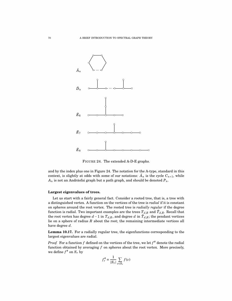
70 A BRIEF INTRODUCTION TO SPECTRAL GRAPH THEORY
An...
Dn...
E6
E7
E8
FIGURE 24. The extended A-D-E graphs.
and by the index plus one in Figure 24. The notation for the A-type, standard in thiscontext, is slightly at odds with some of our notations: An is the cycle Cn+1, whileAn is not an Andrásfai graph but a path graph, and should be denoted Pn.
Largest eigenvalues of trees.
Let us start with a fairly general fact. Consider a rooted tree, that is, a tree witha distinguished vertex. A function on the vertices of the tree is radial if it is constanton spheres around the root vertex. The rooted tree is radially regular if the degreefunction is radial. Two important examples are the trees Td,R and Td,R. Recall thatthe root vertex has degree d−1 in Td,R , and degree d in Td,R; the pendant verticeslie on a sphere of radius R about the root; the remaining intermediate vertices allhave degree d.
Lemma 10.17. For a radially regular tree, the eigenfunctions corresponding to thelargest eigenvalues are radial.
Proof. For a function f defined on the vertices of the tree, we let f # denote the radialfunction obtained by averaging f on spheres about the root vertex. More precisely,we define f # on Sr by
f #r ≡
1
|Sr |∑
v∈Sr
f (v)
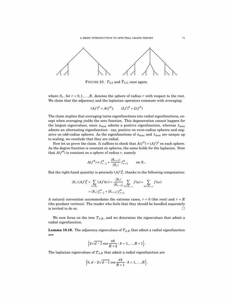
A BRIEF INTRODUCTION TO SPECTRAL GRAPH THEORY 71
FIGURE 25. T3,3 and T3,3, once again.
where Sr, for r = 0,1, . . . ,R, denotes the sphere of radius r with respect to the root.We claim that the adjacency and the laplacian operators commute with averaging:
(Af )# = A( f #), (Lf )# = L( f #)
The claim implies that averaging turns eigenfunctions into radial eigenfunctions, ex-cept when averaging yields the zero function. This degeneration cannot happen forthe largest eigenvalues, since αmax admits a positive eigenfunction, whereas λmax
admits an alternating eigenfunction - say, positive on even-radius spheres and neg-ative on odd-radius spheres. As the eigenfunctions of αmax and λmax are unique upto scaling, we conclude that they are radial.
Now let us prove the claim. It suffices to check that A( f #)= (Af )# on each sphere.As the degree function is constant on spheres, the same holds for the laplacian. Notethat A( f #) is constant on a sphere of radius r, namely
A( f #)≡ f #r−1 +
|Sr+1||Sr |
f #r+1 on Sr .
But the right-hand quantity is precisely (Af )#r , thanks to the following computation:
|Sr | (Af )#r =
∑
v∈Sr
(Af )(v)=|Sr||Sr−1|
∑
u∈Sr−1
f (u)+∑
w∈Sr+1
f (w)
= |Sr| f #r−1 +|Sr+1| f #
r+1
A natural convention accommodates the extreme cases, r = 0 (the root) and r = R(the pendant vertices). The reader who feels that they should be handled separatelyis invited to do so. �
We now focus on the tree Td,R , and we determine the eigenvalues that admit aradial eigenfunction.
Lemma 10.18. The adjacency eigenvalues of Td,R that admit a radial eigenfunctionare
{
2p
d−1 cosπk
R+2: k = 1, . . . ,R+1
}
.
The laplacian eigenvalues of Td,R that admit a radial eigenfunction are
{
0, d−2p
d−1 cosπk
R+1: k = 1, . . . ,R
}
.

72 A BRIEF INTRODUCTION TO SPECTRAL GRAPH THEORY
Proof. Let α be an adjacency eigenvalue admitting a radial eigenfunction f . If fr
denotes the value on the sphere of radius r, then:
α f0 = (d−1) f1
α fr = fr−1 + (d−1) fr+1 r = 1, . . . ,R−1
α fR = fR−1
The solution to this recurrence is a linear combination fr = axr+11 + bxr+1
2 , wherex1 and x2 are the roots of the equation (d−1)x2−αx+1= 0, subject to the initial andterminal conditions f−1 = 0, fR+1 = 0. Thus a+ b = 0 and xR+2
1 = xR+22 . Since x1x2 =
1/(d−1), we find that x1 = ζ/p
d−1 and x2 = ζ/p
d−1, where ζ satisfies ζ2(R+2) = 1.Then
α= (d−1)(x1 + x2)= 2p
d−1 Re(ζ).
Up to multiplication by a scalar, f is given by
fr = (d−1)−r/2 Im(ζr+1), r = 0, . . . ,R.
For f to be non-zero, we have to have ζ 6= ±1. Conversely, if ζ 6= ±1 then f is non-zerosince f0 6= 0. We conclude that the adjacency eigenvalues admitting radial eigenfunc-tions are
{
2p
d−1 Re(ζ) : ζ2(R+2) = 1, ζ 6= ±1}
.
Now let λ be a laplacian eigenvalue admitting a radial eigenfunction g. If gr
denotes, again, the value on the sphere of radius r, then:
(d−1−λ)g0 = (d−1)g1
(d−λ)gr = gr−1+ (d−1)gr+1 r = 1, . . . ,R−1
(1−λ)gR = gR−1
The solution is given by gr = ayr+11 + byr+1
2 , where y1 and y2 are the roots of theequation (d − 1)y2 − (d −λ)y+ 1 = 0, subject to the initial and terminal conditionsg−1 = g0, gR = gR+1. These conditions say that a(y1 − 1) = −b(y2 − 1) and a(y1 −1)yR+1
1 =−b(y2 −1)yR+12 . If y1 = 1 or y2 = 1, then the quadratic relation they satisfy
yields λ= 0, and g is readily seen to be constant. If y1, y2 6= 1 then yR+11 = yR+1
2 . Since
y1 y2 = 1/(d−1), we get y1 = ξ/p
d−1 and y2 = ξ/p
d−1 where ξ2(R+1) = 1. The relationd−λ= (d−1)(y1+ y2) yields
λ= d−2p
d−1 Re(ξ).
Up to re-scaling g, we have gr = (y2−1)yr+11 − (y1−1)yr+1
2 = y1 y2(yr1− yr
2)− (yr+11 −
yr+12 ). Using again the relation y1 y2 = 1/(d−1), and re-scaling g once again, we reach
the formula
gr = (d−1)−r/2 (
Im(ξr)−p
d−1 Im(ξr+1))
, r = 0, . . . ,R.
We note that g is non-zero if and only if ξ 6= ±1. Thus, the laplacian eigenvaluesadmitting radial eigenfunctions are
{
0, d−2p
d−1 Re(ξ) : ξ2(R+1) = 1, ξ 6= ±1}
.
�

A BRIEF INTRODUCTION TO SPECTRAL GRAPH THEORY 73
The eigenvalues of Td,R that we have found are all simple, and there are certainlyother eigenvalues. These are hiding in subtrees. Let us remark, however, that thetree T2,R is the path graph on R + 1 vertices. In this case eigenfunctions are au-tomatically radial, so we actually have all the eigenvalues. The upshot is that theadjacency, respectively the laplacian eigenvalues of Pn, the path graph on n vertices,are
α-spec(Pn)={
2 cosπk
n+1: k = 1, . . . ,n
}
,
λ-spec(Pn)={
2−2 cosπk
n: k = 0, . . . ,n−1
}
.
For our purposes, the main consequence of Lemma 10.18 is that it spells out thelargest eigenvalues of Td,R. Indeed, thanks to Lemma 10.17, we simply have to pickout the largest eigenvalue from each listing.
Theorem 10.19. The largest eigenvalues of Td,R are as follows:
αmax = 2p
d−1 cosπ
R+2, λmax = d+2
pd−1 cos
π
R+1
Using this theorem, we can bound the largest eigenvalues of a tree in terms of themaximal degree and the diameter.
Corollary 10.20. The largest eigenvalues of a tree satisfy
αmax ≤ 2p
d−1 cosπ
δ+2, λmax ≤ d+2
pd−1 cos
π
δ+1.
In particular, αmax < 2p
d−1 and λmax < d+2p
d−1.
Proof. Let X be a tree of maximal degree d and diameter δ. Then X can be viewedas a subtree of Td,δ: pick a path of length δ in X , and then hang X by one of theendpoints. Therefore αmax(X ) ≤ αmax(Td,δ) and λmax(X ) ≤ λmax(Td,δ). The desiredbounds follow from Theorem 10.19. �
For the tree Td,R , we could carry out a spectral analysis as for Td,R , but thecomputations are more cumbersome. We will content ourselves with estimates onthe largest eigenvalues, obtained by exploiting the relationship with Td,R . Namely,Td,R is a subtree of Td,R , and Td,R is a subtree of Td,2R . From Theorem 10.19 wealso deduce the following.
Corollary 10.21. The largest eigenvalues of Td,R satisfy the following bounds:
2p
d−1 cosπ
R+2≤αmax ≤ 2
pd−1 cos
π
2R+2
d+2p
d−1 cosπ
R+1≤λmax ≤ d+2
pd−1 cos
π
2R+1
The function x 7→ cos(π/x), for x ≥ 2, is non-negative and increasing to 1 as x →∞.Elementary calculus shows that 1−cos(π/x) lies between two numerical multiples of1/x2. In asymptotic notation, 1−cos(π/x)=Θ(x−2). So both Td,R and Td,R satisfy
αmax = 2p
d−1−2p
d−1Θ(R−2),
λmax = d+2p
d−1−2p
d−1Θ(R−2).

74 A BRIEF INTRODUCTION TO SPECTRAL GRAPH THEORY
11. MORE EIGENVALUES
In this section, we take a global view on graph spectra. We consider all eigenval-ues, not just the extremal ones.
Eigenvalues of symmetric matrices: Courant - Fischer.
We start with the main tool for understanding eigenvalues of real symmetric ma-trices: the Courant - Fischer minimax formulas. The power and the versatility ofthese formulas will become apparent in subsequent sections.
Let M be a real symmetric n×n matrix, with eigenvalues
µmin =µ1 ≤ . . . ≤µn =µmax.
We have seen in Theorem 10.1 that the extremal eigenvalues can be described interms of the Rayleigh ratio
R( f )=⟨M f , f ⟩⟨ f , f ⟩
as follows:
µmin =minf 6=0
R( f ), µmax = maxf 6=0
R( f )
Broadly speaking, the minimax formulas describe each eigenvalue µk via con-strained optimizations of the Rayleigh ratio.
Theorem 11.1 (Courant - Fischer). The following hold:
µk = mindimV=k
maxf ∈V
R( f )= maxdimW=n−k+1
minf ∈W
R( f )(7)
Furthermore, let f1, f2, . . . , fn be an orthonormal basis of eigenvectors, let Vk denotethe linear span of f1, . . . , fk, and let Wn−k+1 denote the linear span of fk, . . . , fn. Then:
µk = maxf ∈Vk
R( f )= minf ∈Wn−k+1
R( f )(8)
Proof. We start by establishing the ‘local’ formulas (8). If f ∈ Vk then f =∑
i≤k ci f i ,so
R( f )=⟨M f , f ⟩⟨ f , f ⟩
=∑
i≤kµi |ci |2∑
i≤k |ci |2≤µk.
If f ∈Wn−k+1 then f =∑
i≥k ci f i , so
R( f )=⟨M f , f ⟩⟨ f , f ⟩
=∑
i≥kµi |ci |2∑
i≥k |ci |2≥µk.
We conclude by noting that for the eigenvector fk, which is both in Vk and in Wn−k+1,we have R( fk)= µk.
Next, we establish the ‘global’ formulas (7). We clearly have
µk =maxf ∈Vk
R( f )≥ mindimV=k
maxf ∈V
R( f ).
For the reverse inequality, we need to show that µk ≤maxf ∈V R( f ) for each subspaceV of dimension k. We use the following observation: if two subspaces V ,W ⊆C
n sat-isfy dimV+dimW > n, then V and W share a non-zero vector. Hence a k-dimensional

A BRIEF INTRODUCTION TO SPECTRAL GRAPH THEORY 75
space V and the (n−k+1)-dimensional space Wn−k+1 share a non-zero vector f0. Wethen have
µk = minf ∈Wn−k+1
R( f )≤ R( f0)≤maxf ∈V
R( f )
as desired. The second minimax formula is established by a similar argument. �
The min-max formulas for the intermediate eigenvalues are rather unwieldy, evenfor adjacency and laplacian matrices. One refreshing and useful exception is a fairlytransparent formula for λ2, the smallest non-trivial laplacian eigenvalue. The con-stant function 1 is an eigenfunction for the simple eigenvalue λ1 = 0, and the spaceWn−1 from the Courant - Fischer theorem is then the orthogonal complement of thesubspace spanned by 1. We get:
λ2 = min0 6= f ⊥1
⟨Lf , f ⟩⟨ f , f ⟩
=min{
∑
{u,v}∈E
∣
∣f (u)− f (v)∣
∣
2
∑
u∈V | f (u)|2:
∑
u∈Vf (u) = 0, f 6= 0
}
(9)
Exercise 11.2. Show that a graph which is not complete has λ2 ≤ d and α2 ≥ 0.
A bound for the laplacian eigenvalues.
The following result is a bound on the growth of laplacian eigenvalues, formulatedin terms of the maximal degree and the diameter. Two ingredients in the proof arethe minimax formulas, and our discussion around the largest eigenvalues of trees.
Theorem 11.3. Let 1≤ k ≤ δ/2. Then:
λk+1 ≤ d−2p
d−1 cos2πk
δ
Proof. We break down the proof into three steps. In the first one, we construct asample function which is supported on a ball, and whose laplacian Rayleigh ratio iscontrolled in terms of the radius. In the second step, we argue that there are k+1balls which are well-separated. In the last step, we consider global functions on thegraph defined by taking scaled sample functions on each of the k+1 balls.
Step 1. Let BR be a ball of radius R ≥ 0 around a vertex v. We show that there isa non-zero function g supported on BR such that
⟨Lg, g⟩⟨g, g⟩
≤ d−2p
d−1 cosπ
R+2.(∗)
If R = 0, take g to be 1 at v and 0 elsewhere. Then the left-hand side of (∗) isdeg(v) while the right-hand side is d.
Assume R ≥ 1. Consider the tree Td,R , and let αT denote its largest adjacencyeigenvalue. Let f be a positive eigenfunction on Td,R for αT . Since f is radial,we may view it as a function of the radius r 7→ fr, for r = 0, . . . ,R. Spelling out theeigenrelation for f , we get
αT f0 = d f1, αT fr = fr−1+ (d−1) fr+1 for r = 1, . . . ,R
with the convention that fR+1 = 0. These relations, and the fact that αT < d, implythat f is decreasing. Indeed, the first relation yields f0 > f1, while the second relationyields that fr > fr+1 provided fr−1 > fr.
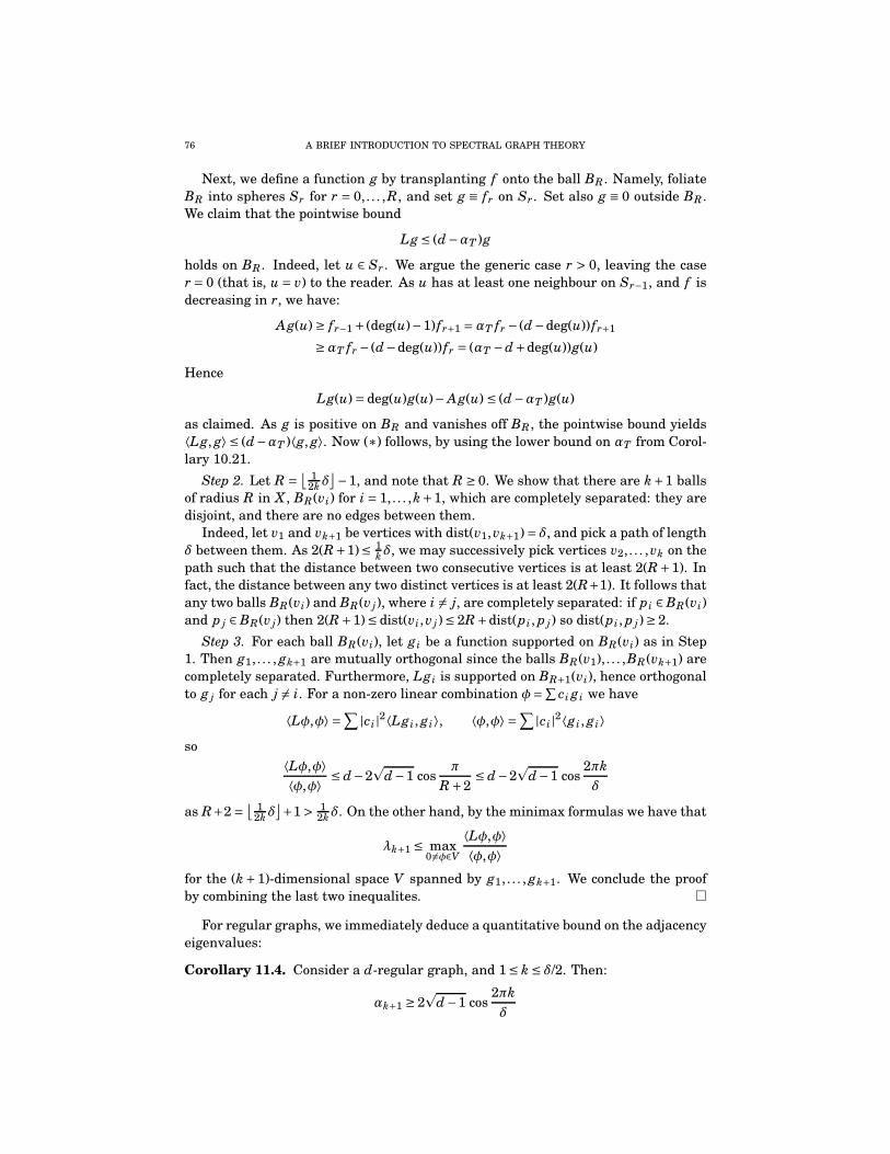
76 A BRIEF INTRODUCTION TO SPECTRAL GRAPH THEORY
Next, we define a function g by transplanting f onto the ball BR . Namely, foliateBR into spheres Sr for r = 0, . . . ,R, and set g ≡ fr on Sr. Set also g ≡ 0 outside BR .We claim that the pointwise bound
Lg ≤ (d−αT )g
holds on BR . Indeed, let u ∈ Sr . We argue the generic case r > 0, leaving the caser = 0 (that is, u = v) to the reader. As u has at least one neighbour on Sr−1, and f isdecreasing in r, we have:
Ag(u) ≥ fr−1 + (deg(u)−1) fr+1 =αT fr − (d−deg(u)) fr+1
≥αT fr − (d−deg(u)) fr = (αT −d+deg(u))g(u)
Hence
Lg(u) = deg(u)g(u)− Ag(u) ≤ (d−αT )g(u)
as claimed. As g is positive on BR and vanishes off BR , the pointwise bound yields⟨Lg, g⟩ ≤ (d−αT )⟨g, g⟩. Now (∗) follows, by using the lower bound on αT from Corol-lary 10.21.
Step 2. Let R =⌊ 1
2kδ⌋
−1, and note that R ≥ 0. We show that there are k+1 ballsof radius R in X , BR(vi) for i = 1, . . . ,k+1, which are completely separated: they aredisjoint, and there are no edges between them.
Indeed, let v1 and vk+1 be vertices with dist(v1,vk+1)= δ, and pick a path of lengthδ between them. As 2(R+1)≤ 1
kδ, we may successively pick vertices v2, . . . ,vk on thepath such that the distance between two consecutive vertices is at least 2(R+1). Infact, the distance between any two distinct vertices is at least 2(R+1). It follows thatany two balls BR(vi) and BR(v j), where i 6= j, are completely separated: if pi ∈BR(vi)and p j ∈ BR(v j) then 2(R+1)≤ dist(vi,v j)≤ 2R+dist(pi , p j) so dist(pi , p j)≥ 2.
Step 3. For each ball BR(vi), let gi be a function supported on BR(vi) as in Step1. Then g1, . . . , gk+1 are mutually orthogonal since the balls BR(v1), . . . ,BR(vk+1) arecompletely separated. Furthermore, Lgi is supported on BR+1(vi), hence orthogonalto g j for each j 6= i. For a non-zero linear combination φ=
∑
ci gi we have
⟨Lφ,φ⟩ =∑
|ci |2⟨Lgi, gi⟩, ⟨φ,φ⟩ =∑
|ci |2⟨gi , gi⟩
so
⟨Lφ,φ⟩⟨φ,φ⟩
≤ d−2p
d−1 cosπ
R+2≤ d−2
pd−1 cos
2πk
δ
as R+2 =⌊ 1
2kδ⌋
+1> 12kδ. On the other hand, by the minimax formulas we have that
λk+1 ≤ max0 6=φ∈V
⟨Lφ,φ⟩⟨φ,φ⟩
for the (k+1)-dimensional space V spanned by g1, . . . , gk+1. We conclude the proofby combining the last two inequalites. �
For regular graphs, we immediately deduce a quantitative bound on the adjacencyeigenvalues:
Corollary 11.4. Consider a d-regular graph, and 1≤ k ≤ δ/2. Then:
αk+1 ≥ 2p
d−1 cos2πk
δ

A BRIEF INTRODUCTION TO SPECTRAL GRAPH THEORY 77
This has, in turn, an interesting qualitative consequence. The diameter of a d-regular graph tends to infinity as the size grows to infinity, and then the above lowerbound tends to 2
pd−1. We obtain:
Corollary 11.5. Fix a threshold t< 2p
d−1. Then α2 > t for all but finitely many d-regular graphs. More generally, for each k ≥ 2 we have that αk > t for all but finitelymany d-regular graphs.
Notes. Naturally, it all happened backwards. First came the last corollary. Thepart concerning α2 is stated in a paper of Alon (Eigenvalues and expanders, Com-binatorica 1986) as a result due Alon and Boppana. Lubotzky, Phillips, and Sarnak(Ramanujan graphs, Combinatorica 1988) proved a weak version of the Alon - Bop-pana result. The first published proof, and a quantitative one, of the Alon - Boppanaresult was subsequently given by Alon’s alter ego Nilli (On the second eigenvalueof a graph, Discrete Math. 1991). Meanwhile, Burger established the general ver-sion in unpublished work (Cheng’s inequality for graphs, preprint 1987). It has beenpointed out by Friedman that the Alon - Boppana phenomenon - namely, escape ofeigenvalues towards 2
pd−1 and beyond - is implicit in work of McKay (The expected
eigenvalue distribution of a large regular graph, Linear Algebra Appl. 1981).Corollary 11.4 came after. The earliest reference is Friedman (Some geometric
aspects of graphs and their eigenfunctions, Duke Math. J. 1993), followed by Quenell(Eigenvalue comparisons in graph theory, Pacific J. Math. 1996) with an independentaccount. See also Nilli (Tight estimates for eigenvalues of regular graphs, Electron.J. Combin. 2004) for a short argument. With some hindsight, the corollary can bealready glimpsed in a paper by Brooks (The spectral geometry of k-regular graphs, J.Anal. Math. 1991)
Theorem 11.3 is essentially due to Urakawa (Eigenvalue comparison theorems ofthe discrete Laplacians for a graph, Geom. Dedicata 1999). Our approach is some-what different, and somewhat simpler. Theorem 11.3 is the graph-theoretic ana-logue of a bound due to Cheng (Eigenvalue comparison theorems and its geometricapplications, Math. Z. 1975) for the laplacian eigenvalues on a compact Riemannianmanifold.
Eigenvalues of symmetric matrices: Cauchy and Weyl.
We now turn to the behaviour of eigenvalues with respect to several operationson symmetric matrices. We discuss two general principles, Cauchy’s interlacing the-orem and Weyl’s inequality. The first one addresses the operation of deleting a rowand the corresponding column. The second one concerns addition. Both results areapplications of the Courant - Fischer minimax formulas.
Theorem 11.6 (Cauchy). Let M′ be the symmetric (n−1)×(n−1) matrix obtained bydeleting the first row and the first column of M. Then the eigenvalues of M′ interlacethe eigenvalues of M:
µ1 ≤µ′1 ≤µ2 ≤ . . . ≤µn−1 ≤µ′
n−1 ≤ µn
Proof. Let φ denote the linear embedding Cn−1
,→ Cn given by adding 0 as first co-
ordinate. Then the Rayleigh ratios of M′ and M are related by the formula R′( f ′) =R(φ( f ′)).
78 A BRIEF INTRODUCTION TO SPECTRAL GRAPH THEORY
We have to show that µk ≤ µ′k ≤µk+1 for k = 1, . . . ,n−1. Now
µ′k = min
dimV ′=kmaxf ′∈V ′
R′( f ′)
= mindimV ′=k
maxf ∈φ(V ′)
R( f )≥ mindimV=k
maxf ∈V
R( f )=µk
and
µ′k = max
dimW′=n−kminf ′∈W′
R′( f ′)
= maxdimW′=n−k
minf ∈φ(W′ )
R( f )≤ maxdimW=n−k
minf ∈W
R( f )=µk+1
as desired. �
Theorem 11.7 (Weyl). Let M and N be symmetric n×n matrices. Then
µk+ℓ−1(M+N) ≥µk(M)+µℓ(N)
as long as the indices satisfy 1≤ k,ℓ,k+ℓ−1 ≤ n.
Proof. If three subspaces U,V ,W ⊆Cn satisfy dimU+dimV +dimW > 2n, then U, V
and W share a non-zero vector. The three subspaces we will use are: the subspaceWn−k+1 with respect to M, the subspace Wn−ℓ+1 with respect to N, and the subspaceVk+ℓ−1 with respect to M+N. For a common non-zero vector f0, we have
µk+ℓ−1(M+N) ≥ RM+N ( f0)= RM( f0)+RN ( f0)≥µk(M)+µℓ(N)
as claimed. �
Weyl’s inequality provides lower and upper bounds for the eigenvalues of M +N,thought of as a perturbation of M by N. Let us single out the simplest bounds of thiskind.
Corollary 11.8. Let M and N be symmetric n×n matrices. Then:
µk(M)+µmin(N)≤µk(M+N) ≤µk(M)+µmax(N)(10)
Proof. The lower bound µk(M)+µmin(N) ≤ µk(M + N) is the case ℓ = 1 of Weyl’s in-equality. Replacing M by M+N, and N by −N, we get µk(M+N)+µmin(−N) ≤µk(M).As µmin(−N) = −µmax(N), this is precisely the upper bound µk(M + N) ≤ µk(M)+µmax(N). �
Here is a simple application to graph eigenvalues. Recall that, for a d-regulargraph, the adjacency and the laplacian eigenvalues are related by αk +λk = d. Ingeneral, αk +λk is confined to the interval determined by the minimal and the max-imal vertex degrees.
Proposition 11.9. We have dmin ≤αk +λk ≤ d.
Proof. We apply the inequality (10) to M = −A, and N = diag(deg), the diagonalmatrix recording the degrees. Thus M + N = L. The relevant eigenvalues are:µk(M) = −αk, µk(M +N) = λk, and µmin(N) = dmin, µmax(N) = d. Thus −αk +dmin ≤λk ≤−αk +d, as desired. �
Exercise 11.10. Let M be a symmetric matrix of size n, partitioned as
M =(
M′ NN t M′′
)
where M′ and M′′ are square, and hence symmetric, matrices of size n′ respectivelyn′′. Show that µ1 +µk+ℓ ≤µ′
k +µ′′ℓ
for 1 ≤ k ≤ n′, 1≤ ℓ≤ n′′.

A BRIEF INTRODUCTION TO SPECTRAL GRAPH THEORY 79
Notes. Proposition 11.9 is an observation of Nikiforov (Eigenvalues and extremaldegrees of graphs, Linear Algebra Appl. 2006). Exercise 11.10 is a finite-dimensionalinstance of a result due to Aronszajn (Rayleigh-Ritz and A. Weinstein methods forapproximation of eigenvalues I. Operators in a Hilbert space, Proc. Nat. Acad. Sci.U. S. A. 1948).
Subgraphs.
How do the eigenvalues of a graph change upon passing to a subgraph? For thelargest adjacency or laplacian eigenvalues, we have addressed this question in The-orem 10.14. We can now extend our scope to the entire spectrum, thanks to theCauchy and Weyl inequalities. In this section, we dispense with the usual connectiv-ity assumption. We maintain, however, the non-degeneracy assumption that n≥ 3.
Starting with an ambient graph, one gets a subgraph by two operations: remov-ing vertices, and removing edges. We will take a close look at each one, proving inparticular the following:
Theorem 11.11. If X ′ is a spanning subgraph of X , then the laplacian eigenvaluessatisfy λ′
k ≤ λk. If X ′ is an induced subgraph of X , then the adjacency eigenvaluessatisfy α′
k ≤αk.
A spanning subgraph is a subgraph having all the vertices of the ambient graph.An induced subgraph is a subgraph having all the edges inherited from the ambientgraph. The above theorem conforms with the philosophy that laplacian eigenvaluessense the edges, while adjacency eigenvalues sense the vertices.
The next two theorems give bounds for both the adjacency and the laplacian eigen-values, when either a vertex or an edge is removed from the ambient graph.
Theorem 11.12. Let X ′ be a graph obtained by removing a vertex from the graphX . Then its adjacency and its laplacian eigenvalues can be bounded as follows:
αk+1 ≤α′k ≤αk(11)
respectively
λk −1 ≤λ′k ≤λk+1(12)
Proof. Label the vertices by 1,2, . . . ,n so that the removed vertex is 1. The adjacencymatrix A′ is obtained by deleting the first row and column of the adjacency matrixA. Cauchy’s interlacing theorem is directly applicable, yielding (11).
The laplacian matrix L′ is given by L′ = M + N, where M denotes the matrixobtained by deleting the first row and column of the laplacian matrix L, and N is thefollowing matrix:
(
−Ideg(1)
0n−1−deg(1)
)
Here deg(1) denotes, as usual, the degree of the vertex 1, and we furthermore assumethat the neighbours of 1 come right after (2, 3 and so on). The smallest eigenvalueof N is −1. The largest is 0, except when deg(1) = n−1 in which case it is −1. By(10), we have µk(M)−1≤λ′
k ≤µk(M) for k = 1, . . . ,n−1. On the other hand, Cauchy’sinterlacing theorem says that λk ≤ µk(M) ≤ λk+1 for k = 1, . . . ,n−1. The two-sidedbounds (12) follow. �

80 A BRIEF INTRODUCTION TO SPECTRAL GRAPH THEORY
Theorem 11.13. Let X ′ be a graph obtained by removing an edge from the graphX . Then its adjacency and its laplacian eigenvalues can be bounded as follows:
αk −1≤α′k ≤αk +1(13)
respectively
λk −2≤λ′k ≤ λk(14)
Proof. Label the vertices by 1,2, . . . ,n so that the removed edge is the one between 1and 2. The adjacency matrix of X ′ and that of X are related by A′ = A+N, where Ais the adjacency matrix of X , and N is the following matrix:
0 −1−1 0
0n−2
This matrix has simple eigenvalues ±1, as well as 0 with multiplicity n− 2. Thebound (10), with n−k in place of k, yields (13).
The laplacian matrix of X ′ and that of X are related by L′ = L+N, where N is thefollowing matrix:
−1 −1−1 −1
0n−2
The eigenvalues of this matrix are −2 with multiplicity 1, and 0 with multiplicityn−1. Now (10) gives (14). �
Revisiting the proof, we see that the adjacency part of the edge-removal theoremcan be generalized.
Theorem 11.14. Let Y be a subgraph of X , and let X ′ be the graph obtained fromX by removing the edges of Y . Then the adjacency eigenvalues of X ′ satisfy thefollowing bounds:
αk −αmax(Y )≤α′k ≤αk −αmin(Y )(15)
Example 11.15. A graph is said to be hamiltonian if it contains a spanning cycle,meaning a cycle that visits every vertex. Graphically, this means that the graph canbe drawn as a cycle with additional chords.
The Petersen graph is not hamiltonian. This can be argued combinatorially, buta spectral proof fits the discussion. Let us assume that the Petersen graph hasa hamiltonian cycle. Such a cycle C10 is obtained by removing 5 edges from thePetersen graph, so we will rely on the edge-removal theorem. Specifically, we coulduse the left-hand bound in (14), saying that λk(C10) ≤ λk(Pet) for all k = 1, . . . ,10.Even better, we can use (15). In this case, Y consists of 5 disjoint copies of K2, so:
αk(Pet)−1≤αk(C10)≤αk(Pet)+1, k = 1, . . . ,10(†)
Note that the right-hand bound of (†) is the laplacian bound mentioned before.Listing the adjacency eigenvalues of C10 and those of the Petersen graph, we find
that (†) fails for k = 6 and k = 7.

A BRIEF INTRODUCTION TO SPECTRAL GRAPH THEORY 81
k 10 9 8 7 6 5 4 3 2 1
αk(C10) −2 −1.6.. −1.6.. −0.6.. −0.6.. 0.6.. 0.6.. 1.6.. 1.6.. 2
αk(Pet) −2 −2 −2 −2 1 1 1 1 1 3
Exercise 11.16. Show that a tree has
λ2 ≤ 2−2cosπ
δ+1.
Deduce that λ2 ≤ 1 with equality if and only if the tree is a star graph.
Notes. A spectral proof of the fact that the Petersen graph is not hamiltonian wasfirst given by Mohar (A domain monotonicity theorem for graphs and Hamiltonicity,Discrete Appl. Math. 1992). A simpler argument, essentially the one explainedabove, was noticed by van den Heuvel (Hamilton cycles and eigenvalues of graphs,Linear Algebra Appl. 1995).
The result of Exercise 11.16 is due to Grone, Merris, and Sunder (The Laplacianspectrum of a graph, SIAM J. Matrix Anal. Appl. 1990).
12. SPECTRAL BOUNDS
The focus of this section is on bounds relating graph eigenvalues to graph invari-ants and other combinatorial properties.
Chromatic number and independence number.
We start with one of the earliest results in spectral graph theory. It gives a spec-tral improvement of the upper bound χ≤ 1+d.
Theorem 12.1 (Wilf). We have χ≤ 1+αmax.
Proof. We argue as in the proof of Theorem 2.2, inducting on the size. Let X ′ be the(possibly disconnected) graph obtained by removing a vertex v of minimal degree.The induction hypothesis, and the inequality α′
max ≤ αmax, imply that X ′ can becoloured using at most 1+αmax colours. Since deg(v) ≤ dave ≤αmax, there is at leastone more colour available to complete the colouring. �
One may wonder whether the even better bound χ≤ 1+dave holds. The above proofdoes not work since dave, unlike d and αmax, may increase by passing to subgraphs.And a counterexample is not hard to find: the graph obtained from Kn by attachinga pendant edge at each vertex has χ= n and dave = 1
2 (n+1).The next result gives a lower bound for the chromatic number in terms of adja-
cency eigenvalues. Recall that non-trivial graphs have αmin < 0.
Theorem 12.2 (Hoffman). We have:
χ≥ 1+αmax
−αmin
82 A BRIEF INTRODUCTION TO SPECTRAL GRAPH THEORY
Proof. Let f be a positive eigenfunction for αmax. Given an independent set of ver-tices, S, we consider the perturbation fS = f +af · 1S where 1S is the characteristicfunction of S, and a ∈R will be chosen later. On the one hand, we have
⟨ fS , fS⟩ = ⟨ f , f ⟩+2a ⟨ f , f ·1S⟩+a2 ⟨ f ·1S , f ·1S⟩
= ⟨ f , f ⟩+ (a2 +2a) ⟨ f , f ·1S⟩.
On the other hand,
⟨AfS , fS⟩ = ⟨Af , f ⟩+2a ⟨Af , f ·1S⟩+a2 ⟨A( f ·1S), f ·1S⟩= ⟨Af , f ⟩+2a ⟨Af , f ·1S⟩
by using the symmetry of A, and the independence of S.Now consider a partition V = S1 ∪·· ·∪Sχ into χ independent subsets, and let fk
be the corresponding modifications of f on each Sk, as above. Adding up the aboverelations, we get:
∑
⟨ fk, fk⟩ = (χ+a2 +2a) ⟨ f , f ⟩∑
⟨Afk, fk⟩ = (χ+2a) ⟨Af , f ⟩ = (χ+2a)αmax ⟨ f , f ⟩
As ⟨Afk, fk⟩ ≥αmin ⟨ fk, fk⟩ for each k, we are led to the following inequality:
(χ+2a)αmax ≥ (χ+a2 +2a)αmin.
Taking now a=−χ, we obtain αmax ≤−(χ−1)αmin. This is the desired inequality. �
Exercise 12.3. Give an alternate proof of the previous theorem by using the resultof Exercise 11.10.
We now turn to the independence number, where we get an upper bound in lapla-cian terms.
Theorem 12.4 (Hoffman). We have:
ι≤ n(
1−dmin
λmax
)
Proof. Let S be a proper subset of vertices, and consider the function f defined byf ≡ |Sc| on S, respectively f ≡−|S| on Sc. We compute
⟨ f , f ⟩ =∑
u∈S
f (u)2 +∑
u∈Scf (u)2 = |S| · |Sc |2 +|Sc| · |S|2 = n|S||Sc |
⟨Lf , f ⟩ =∑
{u,v}∈E| f (u)− f (v)|2 =
∑
{u,v}∈∂S
| f (u)− f (v)|2 = n2|∂S|
and so:⟨Lf , f ⟩⟨ f , f ⟩
=n|∂S||S||Sc |
(16)
Now, if S is an independent subset, then all edges emanating from vertices of S arein ∂S, so |∂S| ≥ dmin |S|. The Rayleigh ratio on the left-hand side of (16) is at mostλmax. Therefore
λmax ≥n dmin
n−|S|that is, |S| ≤ n
(
1−dmin/λmax)
. �
In practice, the previous two theorems are usually applied to regular graphs. Inthis case, they can be stated as follows.

A BRIEF INTRODUCTION TO SPECTRAL GRAPH THEORY 83
Corollary 12.5. For a regular graph, we have:
ι≤n
1−d/αmin, χ≥ 1−d/αmin
For the independence number, we have rewritten the bound of Theorem 12.4 byusing the relation αmin +λmax = d. A practical motivation is that computations usu-ally provide the adjacency eigenvalues. For the chromatic number, we have usedαmax = d in the bound provided by Theorem 12.2. Observe that, in the regular case,the chromatic bound can be derived from the independence bound by using χ · ι≥ n.
In general, the independence bound of Theorem 12.4 and the inequality χ · ι ≥ nimply the following chromatic bound:
χ≥1
1−dmin/λmax
Note, however, that this is no better than the adjacency bound of Theorem 12.2. Asαmax ≥ dave ≥ dmin, and αmin +λmax ≥ dmin, we get
1+αmax
−αmin≥ 1+
dmin
λmax −dmin=
1
1−dmin/λmax.
Example 12.6. Consider the Paley graph P(q), where q ≡ 1 mod 4. Plugging inn= q, d = 1
2 (q−1), and αmin =− 12 (p
q+1) in the previous corollary, we find that
ι≤pq ≤χ.
These are fairly good bounds. As we have seen in Theorem 6.13, equalities hold whenq is a square.
Notes. Theorem 12.1 is due to Wilf (The eigenvalues of a graph and its chromaticnumber, J. London Math. Soc. 1967). Theorem 12.2 is due to Hoffman (On eigenval-ues and colorings of graphs, in ‘Graph Theory and its Applications’, Academic Press1970) but the proof given above is based on an argument of Nikiforov (Chromaticnumber and spectral radius, Linear Algebra Appl. 2007). Hoffman’s original ap-proach is that of Exercise 12.3. Theorem 12.4 is also due to Hoffman (unpublished).
Isoperimetric constant.
The smallest positive eigenvalue of the laplacian, λ2, is an indicator of how wella graph is connected. This principle arises from, and is made quantitative by, re-lations between λ2 and various graph-theoretic measures of connectivity. Here wepursue the relation with the isoperimetric constant β. As we will see, the spectralperspective on β turns out to be particularly successful. It is, in fact, one of themost consistent and conceptual instances of understanding combinatorial aspects byspectral methods.
Theorem 12.7 (Alon - Milman). We have β≥λ2/2.
Proof. Recall (16):
⟨Lf , f ⟩⟨ f , f ⟩
=n|∂S||S||Sc |
84 A BRIEF INTRODUCTION TO SPECTRAL GRAPH THEORY
where S is a proper subset of vertices, and f is the function given by f ≡ |Sc| on S,respectively f ≡−|S| on Sc. As f ⊥ 1, the left-hand side is at least λ2. So, if S is suchthat |S| ≤ n/2, then
λ2 ≤n|∂S||S||Sc |
≤ 2|∂S||S|
implying that β≥λ2/2. �
There is an upper bound of similar flavour, but this is contingent on the existenceof a certain kind of eigenfunction.
Theorem 12.8. If there is a laplacian eigenvalue λ having a {±1}-valued eigenfunc-tion, then β≤λ/2.
Proof. Let g be a {±1}-valued eigenfunction for λ, and let S = {v : g(v)= 1}. As g is or-thogonal to 1, we have |S| = n/2. Now ⟨Lg, g⟩ = 4|∂S| and ⟨g, g⟩ = n= 2|S|. Therefore
λ=⟨Lg, g⟩⟨g, g⟩
= 2|∂S||S|
≥ 2β
as claimed. �
Note that, if λ is to have a {±1}-valued eigenfunction, then λ has to be an eveninteger. Indeed, in the eigenrelation λg(v) = deg(v)g(v)−
∑
u:u∼v g(u), the right-handside is an even integer. Also, n has to be even.
An immediate consequence of the previous two theorems is the following.
Corollary 12.9. If λ2 admits a {±1}-valued eigenfunction, then β=λ2/2.
This criterion for computing the isoperimetric constant is applicable in many ex-amples. Even for those where we already knew β, the spectral approach is more sat-isfactory than our previous combinatorial arguments. One context where we knownot only the eigenvalues, but also corresponding eigenfunctions, is that of Cayleygraphs and bi-Cayley graphs of abelian groups. Some of the examples that followwill exploit that perspective.
Example 12.10. The Petersen graph has λ2 = 2. A corresponding {±1}-valued eigen-function is most easily seen on the standard drawing of the Petersen graph. Put +1on the vertices of the outer pentagon, and −1 on the vertices of the inner pentagram.Thus, β= 1.
Example 12.11. The cube graph Qn has λ2 = 2. Putting +1 on binary strings start-ing in 0, respectively −1 on binary strings starting in 1, defines a {±1}-valued eigen-function for λ2. Hence β= 1.
In fact, for any Cayley graph of (Z2)n we can find a {±1}-valued eigenfunction forλ2. The reason is that λ2 admits some non-trivial character as an eigenfunction, andall non-trivial characters of (Z2)n are {±1}-valued. Thus β= λ2/2, an integer, for anyCayley graph of (Z2)n.
Exercise 12.12. (i) Show that the halved cube graph 12Qn has isoperimetric constant
β = n− 1. (ii) For a fixed n, consider the decked cube graphs DQn(a) for varyinga ∈ (Z2)n. Which choice of a maximizes the isoperimetric constant of DQn(a)?
Example 12.13. Consider now the twin graphs, K4×K4 and the Shrikhande graph.Both have λ2 = 4, and for both graphs we can see a corresponding {±1}-valued eigen-function. In K4 ×K4, we alternatively put +1 and −1 as we circle around the vertex

A BRIEF INTRODUCTION TO SPECTRAL GRAPH THEORY 85
set. In the Shrikhande graph, we put +1 on the vertices of the outer octagon, and −1on all the inner vertices.
Our seemingly lucky choice of eigenfunctions prompts a legitimate concern: whatif the Cheshire Cat takes away our nice picture of, say, the Shrikhande graph? We arethen left with a Cayley graph description, inviting us to take an algebraic approach.And we find that, as in the previous example, more is true: any Cayley graph of(Z4)n admits a {±1}-valued eigenfunction for λ2, and so β = λ2/2. Indeed, λ2 has anon-trivial character χ as an eigenfunction. Now χ takes values in {±1,±i}. The realand imaginary parts of χ, Re(χ) and Im(χ), are eigenfunctions for λ2. So Re(χ)+Im(χ),which is {±1}-valued, is an eigenfunction as well.
Example 12.14. For the incidence graph In(q), we know that
λ2 = d−α2 =qn−1 −1
q−1− qn/2−1.
Our aim is to show that, for suitable q and n, the generic lower bound β ≥ λ2/2becomes an equality.
Let us think of In(q) as the bi-Cayley graph of K∗/F∗ with respect to {[s] : Tr(s) = 0}.Assuming that q is odd, a {±1}-valued multiplicative character of K - in fact, the onlyone - is the quadratic signature σ. If we also assume that n is even, then σ is trivialon F
∗ so it defines a {±1}-valued character, still denoted σ, of K∗/F∗. We now refer tothe arguments of Theorem 9.7 and Example 9.9. As ασ is real, in fact integral, wehave that the adjacency eigenvalue |ασ| = ±ασ has an eigenfunction given by σ onthe black vertices and ±σ on the white vertices. In other words, the second largesteigenvalue α2 = qn/2−1 has a {±1}-valued eigenfunction. We conclude that, for q oddand n even, the incidence graph In(q) has β=λ2/2. As a concrete example, I4(q) hasβ= q2 +1.
The next result is an upper bound for β in terms of λ2 and the maximal degree.
Theorem 12.15 (Dodziuk). We have β≤√
2dλ2.
Proof. We proceed in three steps. The first step is a functional inequality involvingβ. The second step turns the ℓ1 inequality of the first step into an ℓ2 inequality. Inthe third step, we apply the inequality established in the second step to the positivepart of an eigenfunction for λ2.

86 A BRIEF INTRODUCTION TO SPECTRAL GRAPH THEORY
Step 1. Let f be a non-negative function on the graph, supported on no more thanhalf the vertices. Then:
β∑
vf (v)≤
∑
{u,v}∈E| f (u)− f (v)|
Indeed, let 0 = f0 < f1 < . . . < fs be the values taken by f . We write∑
{u,v}∈E| f (u)− f (v)| =
∑
k≥1Nk fk.
The coefficients are given by
Nk = E(
{f = fk},{f < fk})
−E(
{f = fk},{f > fk})
where, say, E(
{f = fk},{f > fk})
denotes the number of edges between the vertexsubsets {v : f (v)= fk} and {v : f (v)> fk}. We then have
Nk = E(
{f ≥ fk},{f < fk})
−E(
{f ≤ fk},{f > fk})
= |∂{f ≥ fk}|− |∂{f ≥ fk+1}|
so∑
k≥1Nk fk =
∑
k≥1
(
|∂{f ≥ fk}|− |∂{f ≥ fk+1}|)
fk
=∑
k≥1|∂{f ≥ fk}| ( fk − fk−1).
At this point, we can bring in β. For each k ≥ 1, the set {f ≥ fk} contains no morethan half the vertices, so |∂{f ≥ fk}| ≥β |{f ≥ fk}|. Therefore
∑
k≥1Nk fk ≥β
∑
k≥1|{f ≥ fk}| ( fk − fk−1)
=β∑
k≥1
(
|{f ≥ fk}|− |{f ≥ fk+1}|)
fk
=β∑
k≥1|{f = fk}| fk =β
∑
f (v)
as claimed.
Step 2. Let f be a real-valued function, supported on no more than half the ver-tices. Then:
β2 ⟨ f , f ⟩ ≤ 2d ⟨Lf , f ⟩
Indeed, the bound from Step 1, applied to f 2, says that
β∑
vf (v)2 ≤
∑
{u,v}∈E
∣
∣ f 2(u)− f 2(v)∣
∣.
Now | f 2(u)− f 2(v)| = | f (u)− f (v)| · | f (u)+ f (v)| and so, by Cauchy - Schwarz, we have:(
∑
{u,v}∈E
∣
∣ f 2(u)− f 2(v)∣
∣
)2≤
(
∑
{u,v}∈E
∣
∣ f (u)− f (v)∣
∣
2) (
∑
{u,v}∈E
∣
∣f (u)+ f (v)∣
∣
2)
The first factor on the right-hand side is ⟨Lf , f ⟩. We bound the second factor asfollows:
∑
{u,v}∈E
∣
∣f (u)+ f (v)∣
∣
2 ≤ 2∑
{u,v}∈E
(
f (u)2 + f (v)2)
= 2∑
vdeg(v) f (v)2 ≤ 2d
∑
vf (v)2
The inequalities combine to give β2 ⟨ f , f ⟩2 ≤ 2d ⟨Lf , f ⟩ ⟨ f , f ⟩. The claim follows aftercancelling ⟨ f , f ⟩.

A BRIEF INTRODUCTION TO SPECTRAL GRAPH THEORY 87
Step 3. Let g be an eigenfunction for λ2. By taking the real or the imaginarypart, we may assume that g is real-valued. Let us refer to a vertex v as positive (ornegative) if g(v) > 0 (respectively g(v) < 0). As g is orthogonal to 1, there are bothpositive and negative vertices. Up to replacing g by −g, we may assume that nomore than half the vertices are positive. Let f be the positive part of g, that is thefunction defined by f = g on positive vertices, and f = 0 elsewhere. Then f (v)≥ g(v)for every vertex v, and so Af (v)≥ Ag(v) for every vertex v. At a positive vertex v wehave
Lf (v)= deg(v) f (v)− Af (v)≤ deg(v) g(v)− Ag(v)= Lg(v).
As f is supported on the positive vertices, where it takes positive values by definition,we have
⟨Lf , f ⟩ ≤ ⟨Lg, f ⟩ =λ2 ⟨g, f ⟩ = λ2 ⟨ f , f ⟩.
Combining this bound with the bound from Step 2, we conclude that β2 ≤ 2dλ2. �
The spectral lower bound for β (Theorem 12.7) had a very easy proof, and turnedout to be very effective in practice. So it is quite ironic that the spectral upper boundof Theorem 12.15, which is significantly harder to prove, is rarely effective in prac-tice. Tested on some families of graphs, it quickly appears to be a fairly bad bound.Both the Paley graphs P(q) and the incidence graphs I3(q) have α2 ∼ C
pd as q →∞,
for some numerical constant C. Thus λ2 = d−α2 ∼ d, and√
2dλ2 ∼p
2d as q →∞.This is worse than the trivial upper bound d. On the cubes Qn, the performance isalso poor: the spectral upper bound is
√
2dλ2 = 2p
d, whereas β= 1. Here, at least,we are beating the combinatorial upper bound of roughly d/2.
On the other hand, the spectral upper bound is effective for the cycles Cn: hereβ∼ 4/n and
√
2dλ2 = 4sin(π/n) ∼ 4π/n. Unlike the previous families, the cycles haveconstant degree.
Recall that an expander family is a d-regular family of graphs whose isoperi-metric constant is uniformly bounded away from 0. The conceptual importance ofTheorem 12.15 is that, in conjunction with Theorems 12.7, it implies the following:a d-regular family is an expander family if and only if it has a uniform spectralgap. In laplacian terms, this means that λ2 is uniformly bounded away from 0; inadjacency terms, α2 is uniformly bounded away from d. Note, however, that thereis a quantitative difference between the combinatorial and the spectral approach toexpanders.
Notes. Fiedler (Algebraic connectivity of graphs, Czechoslovak Math. J. 1973) wasthe first to seize the importance of λ2 in relation to graph connectivity. He called λ2
the ‘algebraic connectivity’ of a graph. Fiedler’s starting point was the observationthat, in the context of possibly disconnected graphs, the connectivity of a graph isequivalent to the condition that λ2 > 0.
Theorems 12.7 and 12.15 are graph-theoretic analogues of results due to Cheeger(A lower bound for the smallest eigenvalue of the Laplacian, in ‘Problems in anal-ysis’, Princeton Univ. Press 1970) and Buser (A note on the isoperimetric constant,Ann. Sci. École Norm. Sup. 1982), relating the isoperimetric constant of a compactRiemannian manifold M to the first positive eigenvalue of the laplacian operatoron L2(M). Theorem 12.7 is implicitly due to Alon and Milman (λ1, isoperimetricinequalities for graphs, and superconcentrators, J. Combin. Theory Ser. B 1985).
88 A BRIEF INTRODUCTION TO SPECTRAL GRAPH THEORY
Theorem 12.15, the analogue of Cheeger’s result, is due to Dodziuk (Difference equa-tions, isoperimetric inequality and transience of certain random walks, Trans. Amer.Math. Soc. 1984). See also Mohar (Isoperimetric numbers of graphs, J. Combin.Theory Ser. B 1989) for an improvement.
Expander families do not come easily. The first explicit construction is due toMargulis (Explicit constructions of expanders, Problems Inform. Transmission 1973)and it relies on a rather sophisticated phenomenon, namely Kazhdan’s property (T).The spectral perspective on expanders originates here.
Another early explicit construction of an expander family is due to Buser (On thebipartition of graphs, Discrete Appl. Math. 1984). Buser’s construction also dependson a spectral perspective, but in a rather different way: as he puts it, his proof is“very unorthodox–from the point of view of graph theory–and is in the realm of thespectral geometry of the Laplace operator on Riemann surfaces”.
Remarkably, there are expander families consisting of d-regular graphs with thefollowing property:
(∗) all eigenvalues different from ±d lie in the interval [−2p
d−1,2p
d−1]
In light of the Alon - Boppana phenomenon, one cannot pack the eigenvalues of ad-regular family in a smaller interval. On the other hand, the existence of expanderfamilies satisfying (∗) shows that the Alon - Boppana phenomenon is sharp.
Expander families satisfying (∗) were first constructed by Lubotzky, Phillips, Sar-nak (Ramanujan graphs, Combinatorica 1988) and, independently, Margulis (Ex-plicit group-theoretic constructions of combinatorial schemes and their applicationsin the construction of expanders and concentrators, Problems Inform. Transmission1988). The graphs in question are Cayley graphs of PSL2(Zp) or PGL2(Zp), of degreeℓ+1. Here p and ℓ are distinct primes congruent to 1 mod 4, and the choice of PSL2
or PGL2 depends on the sign of the Legendre symbol (p/ℓ) = (ℓ/p). The proof of (∗) forthese specific graphs rests on a deep number-theoretical fact, the solution of the so-called Ramanujan conjecture. For this reason, expander families satisfying (∗) havecome to be known as Ramanujan expander families. Simpler and more flexible con-structions of Ramanujan expander families are currently known. A very recent andmost notable result of Marcus, Spielman, and Srivastava (Interlacing families I: Bi-partite Ramanujan graphs of all degrees, Ann. of Math. 2015) says that Ramanujanexpander families can be constructed for all degrees greater than 2.
Edge-counting.
Let S and T be two sets of vertices in a regular graph. Denote by e(S,T) thenumber of edges connecting vertices in S to vertices in T, with the convention thatedges having both endpoints in S∩T are counted twice. We want to estimate thelocal quantity e(S,T) in terms of the size of S, the size of T, and global informationon the graph. It turns out that the spread of the non-trivial eigenvalues of X can beused to control the deviation of e(S,T) from its expected value, (edge density) · |S||T|.
We first do this in the bipartite case.
Theorem 12.16. Let X be a bipartite, d-regular graph of half-size m, and let S andT be vertex subsets lying in different sides of the bipartition. Then:
∣
∣
∣e(S,T)−d
m|S||T|
∣
∣
∣≤α2
m
√
|S||T|(
m−|S|)(
m−|T|)
(17)

A BRIEF INTRODUCTION TO SPECTRAL GRAPH THEORY 89
In particular, we have
∣
∣e(S,T)−κ|S||T|∣
∣≤α2
√
|S||T| wheneverd−α2
m≤ κ≤
d+α2
m.(18)
The constant κ in (18) should be thought of as a rounding constant. A genericchoice is κ= d/m, but more convenient choices are usually available in applications.
Proof. Note first that, for the characteristic functions of S and T, we have
⟨A 1S ,1T ⟩ =∑
u∼v1S(u) 1T (v)= e(S,T).
Next, we seek a spectral understanding of the left-hand side. Let
d =α1 >α2 ≥ . . .≥αn−1 =−α2 >αn =−d
be the adjacency eigenvalues of X , where n = 2m denotes, as usual, the number ofvertices. Let also {fk} be an orthonormal basis consisting of normalized adjacencyeigenfunctions. Thus f1 is constant equal to 1/
pn while fn is 1/
pn on, say, black
vertices, and −1/p
n on white vertices. Expand 1S and 1T in the eigenbasis as 1S =∑
sk fk, respectively 1T =∑
tk fk. Then:
⟨A 1S ,1T⟩ =n∑
k=1αksk tk
We separate the terms corresponding to the extremal eigenvalues ±d, and the termscorresponding to the intermediate eigenvalues. If, say, S consists of black verticesand T consists of white vertices, then the extremal coefficients are
s1 =1p
n|S| = sn, t1 =
1p
n|T| = −tn
and so
α1s1 t1 +αnsntn =d
m|S||T|.
For the intermediate coefficients, we note that
n−1∑
k=2|sk |2 = ⟨1S ,1S⟩− |s1 |2 −|sn|2 = |S|−
|S|2
m=
1
m|S|(m−|S|)
and similarly for the coefficients of T. Therefore, by Cauchy - Schwarz we have that
n−1∑
k=2|sk ||tk | ≤
1
m
√
|S||T|(m−|S|)(m−|T|).
Now∣
∣
∣e(S,T)−d
m|S||T|
∣
∣
∣=∣
∣
∣
n−1∑
k≥2αksk tk
∣
∣
∣≤n−1∑
k≥2|αk ||sk ||tk | ≤α2
n−1∑
k≥2|sk ||tk |
and (17) follows. Finally, using√
(m−|S|)(m−|T|) ≤ m−√
|S||T| we get
d+α2
m|S||T|−α2
√
|S||T| ≤ e(S,T)≤d−α2
m|S||T|+α2
√
|S||T|
which implies (18). �
The non-bipartite case can be easily derived.

90 A BRIEF INTRODUCTION TO SPECTRAL GRAPH THEORY
Corollary 12.17. Let X be a non-bipartite, d-regular graph of size n, and let S andT be vertex subsets. Then:
∣
∣
∣e(S,T)−d
n|S||T|
∣
∣
∣≤α
n
√
|S||T||Sc ||T c|, α := max{α2,−αn}
Proof. Let X ′ be the bipartite double of X . Then α = max{α2,−αn} is the secondlargest eigenvalue of X ′. Viewing S and T as vertex subsets of X ′ of different colours,we may apply (17) to get the claimed bound. �
Theorem 12.16 provides a versatile method with numerous combinatorial appli-cations.
Example 12.18. Let F be a finite field with q elements, and let A,B,C,D ⊆ F. Thequestion we wish to address is that of estimating the number of solutions (a,b, c,d) ∈A×B×C×D to the following two equations: a+b = cd, respectively ab+ cd = 1.
The hypersurface {x+ y = zt} ⊆ F4 has q3 = 1
q |F4| points, while the hypersurface
{xy+ zt = 1} ⊆ F4 has (q2 −1)(q−1) ∼ 1
q |F|4 points. So, for both equations we would
expect about 1q |W | solutions in the ‘window’ W := A×B×C×D ⊆ F
4. We will now show
that the error in making this estimate is on the order ofp|W |. More precisely, we
show that the number of restricted solutions NW to either one of the two equationssatisfies the following bound:
∣
∣
∣NW −1
q|W |
∣
∣
∣≤√
q|W |
We work in the incidence graph I3(q), which has m = q2+ q+1, d = q+1, α2 =p
qso we may use κ= 1/q in (18).
For the equation a+b = cd, let S be the set of black vertices of the form [(a,−1, c)]•with a ∈ A and c ∈ C, and let T be the set of white vertices of the form [(−1,b,d)]◦with b ∈ B and d ∈ D. Thus |S||T| = |A||C||B||D| = |W |. Furthermore, there is an edgebetween [(a,−1, c)]• and [(−1,b,d)]◦ precisely when a+ b = cd, so e(S,T) counts thenumber of solutions in W = A×B×C×D to the equation a+ b = cd. An applicationof (18) yields the desired estimate.
For the equation ab+ cd = 1, take S to be the set of black vertices of the form[(1,a, c)]• with a ∈ A and c ∈ C, and T to be the set of white vertices of the form[(−1,b,d)]◦ with b ∈ B and d ∈ D.
Instead of the incidence graph I3(q), we could have used just as well the sum-product SP(q) to handle the equation a+ b = cd. For the equation ab+ cd = 1, how-ever, no perfectly tailored graph is apparent.
Example 12.19. Let F be a field with q elements, where q is odd. Assume thatA,B ⊆ F have the property that the sum-set A+B = {a+ b : a ∈ A,b ∈ B} consists ofsquares. Then |A||B| ≤ q.
Consider the bi-Cayley graph of the additive group of F with respect to F2, the
subset of squares. Recall, this is a bipartite graph whose vertex set consists of twocopies of F, in which an edge connects x• to y◦ whenever x+ y is a square. The givensubsets define a copy of the complete bipartite graph K|A|,|B|, by viewing A and B asvertex subsets of different colours.
The next step is a rather general application of (18): if a regular bipartite graphcontains the complete bipartite graph Ks,t, then
pst ≤
m
1+ (m−d)/α2.(19)

A BRIEF INTRODUCTION TO SPECTRAL GRAPH THEORY 91
Our graph has m = q and d = 12 (q+1). We claim that α2 ≤ 1
2 (p
q+1). Using thesevalues in (19), we obtain st≤ q after a short and pleasant computation.
The bi-Cayley graph we are considering is a close relative of the bi-Paley graph. Inorder to estimate the adjacency eigenvalues, we adapt the arguments of Example 9.8.Let ψ be a non-trivial additive character. Then
αψ =∑
s∈F2
ψ(s) = 1+∑
s∈F∗2
ψ(s) =1
2
(
G(ψ,σ)+1)
.
Hence
|αψ| ≤1
2
(
|G(ψ,σ)|+1)
=1
2(p
q+1)
as claimed.
Exercise 12.20. Let F be a field with q elements, and assume that a proportionc ∈ (0,1) of lines, respectively planes in F
3, is selected. Give a lower bound for c, interms of q, guaranteeing that some selected line is contained in some selected plane.
The edge-counting estimates from 12.16 can be easily extended, mutatis mutan-dis, to path-counting. For two vertex subsets S and T in a graph, we denote bypℓ(S,T) the number of paths of length ℓ connecting vertices in S to vertices in T.
Theorem 12.21. Let X be a bipartite d-regular graph of half-size m, and let S andT be vertex subsets. Assume that either ℓ is odd, and S and T have different colours,or ℓ is even, and S and T have the same colour. Then:
∣
∣
∣pℓ(S,T)−dℓ
m|S||T|
∣
∣
∣≤αℓ
2
m
√
|S||T|(
m−|S|)(
m−|T|)
Corollary 12.22. Let X be a non-bipartite d-regular graph of size n, and let S andT be vertex subsets. Then:
∣
∣
∣pℓ(S,T)−dℓ
n|S||T|
∣
∣
∣≤αℓ
n
√
|S||T||Sc ||T c|, α := max{α2,−αn}
Exercise 12.23. Prove the following diameter bounds. If X is a d-regular graph ofsize n, then
δ≤log(n−1)
log(d/α)+1, α := max{α2,−αn}.
If X is a bipartite d-regular graph of half-size m, then
δ≤log(m−1)
log(d/α2)+2.
Notes. Theorem 12.16 and Corollary 12.17 are slight variations on a result dueto Alon and Chung (Explicit construction of linear sized tolerant networks, DiscreteMath. 1988). A conceptual precursor is Thomason’s notion of jumbled graph (Pseu-dorandom graphs, in ’Random graphs ’85’, North-Holland 1987).
The estimates in Example 12.18 are inspired by, and partially improve, estimatesdue to Gyarmati and Sárközy (Equations in finite fields with restricted solution setsII (Algebraic equations), Acta Math. Hungar. 2008).
Exercise 12.23 is a result due to Chung (Diameters and eigenvalues, J. Amer.Math. Soc. 1989).

92 A BRIEF INTRODUCTION TO SPECTRAL GRAPH THEORY
– FURTHER READING –
Noga AlonTools from higher algebra, in ‘Handbook of combinatorics’, 1749–1783, Elsevier 1995
László Babai, Peter FranklLinear algebra methods in combinatorics, Preliminary version, University of Chicago1992
Simeon BallFinite geometry and combinatorial applications, London Mathematical Society Stu-dent Texts no. 82, Cambridge University Press 2015
Béla BollobásModern graph theory, Graduate Texts in Mathematics no. 184, Springer 1998
Andries E. Brouwer, Willem H. HaemersSpectra of graphs, Universitext, Springer 2012
Peter J. Cameron, Jack H. van LintDesigns, graphs, codes and their links, London Mathematical Society Student Textsno. 22, Cambridge University Press 1991
Fan ChungSpectral graph theory, CBMS Series in Mathematics no. 92, American MathematicalSociety 1997
Giuliana Davidoff, Peter Sarnak, Alain ValetteElementary number theory, group theory, and Ramanujan graphs, London Mathe-matical Society Student Texts no. 55, Cambridge University Press 2003
Chris Godsil, Gordon RoyleAlgebraic graph theory, Graduate Texts in Mathematics no. 207, Springer 2001
Shlomo Hoory, Nathan Linial, Avi WigdersonExpander graphs and their applications, Bull. Amer. Math. Soc. 43 (2006), no. 4,439–561
Jirí MatoušekThirty-three miniatures. Mathematical and algorithmic applications of linear alge-bra, Student Mathematical Library no. 53, American Mathematical Society 2010
Daniel SpielmanSpectral graph theory, in ‘Combinatorial scientific computing’, 495–524, CRC Press2012