A Basin- to Channel-Scale Unstructured Grid Hurricane ...

A Basin- to Channel-Scale Unstructured Grid Hurricane Storm Surge Model Appliedto Southern Louisiana

JOANNES J. WESTERINK,* RICHARD A. LUETTICH,� JESSE C. FEYEN,*,�� JOHN H. ATKINSON,*,##

CLINT DAWSON,# HUGH J. ROBERTS,*,@@ MARK D. POWELL,@ JASON P. DUNION,& ETHAN J. KUBATKO,*AND HASAN POURTAHERI**

*Department of Civil Engineering and Geological Sciences, University of Notre Dame, Notre Dame, Indiana� Institute of Marine Sciences, University of North Carolina at Chapel Hill, Chapel Hill, North Carolina

# Institute for Computational Engineering and Sciences, University of Texas at Austin, Austin, Texas@Hurricane Research Division, National Oceanic and Atmospheric Administration, Miami, Florida

&University of Miami–NOAA/Cooperative Institute for Marine and Atmospheric Studies, National Oceanic andAtmospheric Administration, Miami, Florida

**U.S. Army Corps of Engineers, New Orleans District, New Orleans, Louisiana

(Manuscript received 7 July 2006, in final form 20 June 2007)

ABSTRACT

Southern Louisiana is characterized by low-lying topography and an extensive network of sounds, bays,marshes, lakes, rivers, and inlets that permit widespread inundation during hurricanes. A basin- to channel-scale implementation of the Advanced Circulation (ADCIRC) unstructured grid hydrodynamic model hasbeen developed that accurately simulates hurricane storm surge, tides, and river flow in this complex region.This is accomplished by defining a domain and computational resolution appropriate for the relevantprocesses, specifying realistic boundary conditions, and implementing accurate, robust, and highly parallelunstructured grid numerical algorithms.

The model domain incorporates the western North Atlantic, the Gulf of Mexico, and the Caribbean Seaso that interactions between basins and the shelf are explicitly modeled and the boundary conditionspecification of tidal and hurricane processes can be readily defined at the deep water open boundary. Theunstructured grid enables highly refined resolution of the complex overland region for modeling localizedscales of flow while minimizing computational cost. Kinematic data assimilative or validated dynamic-modeled wind fields provide the hurricane wind and pressure field forcing. Wind fields are modified toincorporate directional boundary layer changes due to overland increases in surface roughness, reductionin effective land roughness due to inundation, and sheltering due to forested canopies. Validation of themodel is achieved through hindcasts of Hurricanes Betsy and Andrew. A model skill assessment indicatesthat the computed peak storm surge height has a mean absolute error of 0.30 m.

1. Introduction

The geography of southern Louisiana is defined by alow-lying coastal floodplain situated adjacent to a

broad continental shelf. A large delta has been formedby the Mississippi River that extends nearly to the con-tinental shelf break. The region is covered by intercon-nected sounds, bays, marshes, lakes, rivers, inlets, andchannels, while the major relief is defined by featuressuch as barrier islands, salt domes, river banks, and anextensive system of levees and raised roads and rail-roads. The region is changing significantly in time dueto natural morphological evolution, man-made levees,and other processes that have led to a sediment-starveddelta that is slowly subsiding (Coleman et al. 1998). Thelow-lying topography, the ubiquitous water bodies, andthe intricate system of raised features make the regionvery susceptible to flooding from hurricane stormsurge. Hurricane surges can propagate rapidly across

�� Current affiliation: Coast Survey Development Labora-tory, National Oceanic and Atmospheric Administration, SilverSpring, Maryland.

## Current affiliation: Ayres Associates, Fort Collins, Colora-do.

@@ Current affiliation: Arcadis U.S., Denver, Colorado.

Corresponding author address: Joannes Westerink, Dept. ofCivil Engineering and Geological Sciences, University of NotreDame, 156 Fitzpatrick Hall, Notre Dame, IN 46556.E-mail: [email protected]

MARCH 2008 W E S T E R I N K E T A L . 833

DOI: 10.1175/2007MWR1946.1

© 2008 American Meteorological Society

MWR3570

the floodplain from many directions and can developdramatic localized amplification due to the topographyand raised features. This geometrically and hydrody-namically complex region is one of the most challengingareas in the world to correctly model hurricane-inducedflooding.

Coastal flooding is driven by wind, atmospheric pres-sure gradients, tides, river flow, short-crested windwaves, and rainfall. A numerical model of coastal in-undation requires an accurate description of the geo-graphic system, process dynamics, forcing mechanisms,and far-field boundary conditions. These issues areclosely related and depend upon domain selection,model physics, the computational resolution of local-scale geography and energetic flow processes, numeri-cal algorithms, and the speed of the software and hard-ware.

We have developed an unstructured-grid finite-element hydrodynamic model to simulate coupledstorm surge, tides, and riverine flow in southern Loui-siana. We emphasize an accurate description of the re-gion’s topography, bathymetry, predominant physicalfeatures, and flow dynamics. The model incorporates abasin-scale domain that simplifies specification of theopen-ocean boundary condition for both tides andstorm surge (Blain et al. 1994; Westerink et al. 1994a),while providing high resolution within regions of rap-idly varying geometry and flow response. Applicationof unstructured grids to resolve the energetic scales ofmotion on a localized basis enables an accurate solutionof the governing equations while minimizing the num-ber of computational nodes. Tides and surge waves cantypically be coarsely resolved in deep waters while re-quiring finer resolution on the shelf (Luettich and Wes-terink 1995; Blain et al. 1998). Furthermore, it is clearthat resolution of critical small-scale features such asinlets, rivers, and navigation channels is necessary inthe coastal floodplain.

The physical processes in the hydrodynamic modelare described by the depth-averaged shallow-waterequations (SWE). These equations are widely used todescribe coupled storm surge, tides, and riverine flowsin the coastal ocean and adjacent floodplain. Processesthat exist at the physical boundaries of the water col-umn and on the subgrid scale are parameterized; theseinclude bottom shear stress, momentum diffusion, free-surface shear stress due to winds, and subgrid-scale ob-structions such as levees. Meteorological forcing is op-timized through application of either data-assimilatedwind fields or validated wind models. Modification ofhurricane wind fields by land roughness has been in-cluded by quantifying the wind boundary layer adjust-

ment through an upwind directional land roughness pa-rameterization, by adjusting land roughness accordingto the depth of local inundation, and by accounting forthe existence of heavily forested canopies.

To validate the model, we have hindcast HurricanesBetsy (1965) and Andrew (1992). These were welldocumented, powerful storms that resulted in wide-spread flooding in southeastern Louisiana. We did notperform any model tuning by adjusting model param-eters but did implement selective intrasimulation gridrefinement and improvements in the definition of thetopography, bathymetry, raised features, and channelsin order to improve the quality of the hindcasts. Allsubgrid-scale processes, including bottom friction coef-ficient, air–sea momentum transfer, and levee weir co-efficients, were selected based on standard values thatare widely used in engineering practice and literature.While geographic and grid refinement improve thequality of the solution, they do not constitute modeltuning since this refinement process more accuratelydefines the existing physical system and flow fields andis an ordered converging process. An assessment wasmade of the model’s skill by comparing measured andcomputed hydrographs and high-water marks.

2. Domain definition and unstructured griddevelopment

Our southern Louisiana storm surge model domainincludes the western North Atlantic, the Gulf ofMexico, and the Caribbean Sea. The domain (Fig. 1)has a geometrically simple and primarily deep-wateropen-ocean boundary that lies along the 60°W meridian(Westerink et al. 1994a; Blain et al. 1994; Mukai et al.2002). The tidal response on this boundary is domi-nated by the astronomical constituents, nonlinear en-ergy is limited due to the large depth, and the boundaryis not located in a resonant basin or near tidal am-phidromes. Hurricane storm surge response along thisboundary is essentially an inverted barometer pressureeffect computed using the atmospheric pressure deficit;it can therefore be easily specified. This boundary al-lows the model to accurately capture basin-to-basin andbasin-to-shelf physics associated with tide- and hurri-cane-driven events.

Much of the domain is bordered by a land boundarymade up of the eastern coastlines of North, Central,and South America. In southern Louisiana the domainincludes a large overland region (Figs. 1–3; see alsoTable 1). The land boundary extends inland and runsalong major hydraulic controls including Interstate 10and U.S. Route 190 in the western part of the state, theentire Atchafalaya flood basin to Simmesport in the

834 M O N T H L Y W E A T H E R R E V I E W VOLUME 136

central part of the state, and Interstates 12/10 north ofLake Pontchartrain in the eastern part of the state.

The domain includes critical hydraulic features andcontrols that both enhance and attenuate storm surge.

We have incorporated the Mississippi River up toBaton Rouge and the Atchafalaya River up to Sim-mesport since both locations have available reliable wa-ter surface elevation gauge data and have adjacent to-

FIG. 1. Western North Atlantic, Gulf of Mexico, and Caribbean Sea computationaldomain with bathymetry (m).

FIG. 2. Detail of bathymetry and topography (m) across southeastern LA, with raised features shown in brown.Geographic locations of interest are indicated by numbers identified in Table 1.


Fig 1 live 4/C Fig 2 live 4/C

pography that is not susceptible to hurricaneinundation. In addition, major dredged navigation ca-nals including the Gulf Intracoastal Waterway(GIWW), the Inner Harbor Navigation Canal (IHNC),the Mississippi River Gulf Outlet (MRGO), Chef Men-teur Pass, the Rigolets, and lakes and bays includingLake Pontchartrain, Lake Maurepas, Lake Borgne,Barataria Bay, Timbalier Bay, Terrebonne Bay, Ver-million Bay, Calcasieu Lake and Sabine Lake are rep-resented. We note that the interconnectivity betweenthe various water bodies significantly impacts water lev-els throughout the system. For example, the Rigoletsand Chef Menteur Pass, connecting Lake Borgne andLake Pontchartrain, as well as Pass Manchac, connect-ing Lake Pontchartrain and Lake Maurepas, providesignificant hydraulic connectivity between these lakesand tend to lower water levels in the lakes to the eastwhile raising water levels in the lakes to the west.

The federal levee system, interstate and state high-ways, and railroads that are elevated above the sur-rounding topography and that are not on piles act ashydraulic controls and have been included as weirs. Thelevee and raised topographic systems surround manyrivers, lakes, and cities including the Mississippi River,the western shore of Lake Pontchartrain, the city ofNew Orleans and the channels that intersect it, as wellas the area around the Atchafalaya flood basin. Federallevees and roads are defined with crown heights as theyexisted in 1965 for the Hurricane Betsy hindcast and as

they existed in 2002 for the Hurricane Andrew hind-cast. We note that the levees around St. Bernard andNew Orleans East in particular were either built orsubstantially raised after Hurricane Betsy in 1965. Wenote that the Mississippi River levees tend to hydrau-lically isolate the east and west banks for all but thelargest storms. However, the configuration of the riverlevees does allow for large surges to develop and propa-gate up river. Furthermore, flood controls such as theBonne Carre Spillway can affect the connectivity be-tween the river and Lake Pontchartrain, although forthe low-river stages that occurred during the storms weexamined, this structure was kept closed.

Bathymetric and topographic data were obtainedfrom a variety of sources. The 5� Gridded Earth To-pography (ETOPO5) database was used to providebathymetric values in deep water as well as in non-U.S.areas (National Geophysical Data Center 2006). InU.S. continental shelf waters, the National Oceanic andAtmospheric Administration (NOAA) depth soundingdatabase was used (National Geophysical Data Center1998). Within southern Louisiana, U.S. Geological Sur-vey (USGS) topographic survey values were applied(U.S. Geological Survey 2006). The depths of navigablerivers and channels were obtained from the U.S. ArmyCorps of Engineers New Orleans District (USACE-MVN) and dredging contractor surveys. An element-based gathering–averaging procedure that sums and av-erages all surface elevation data located within a cluster

FIG. 3. Detail of bathymetry and topography (m) across metropolitan New Orleans and Lake Pontchartrain, withraised features shown in brown. Geographic locations of interest are indicated by numbers identified in Table 1.


Fig 3 live 4/C

of finite elements surrounding a given node was used tointerpolate these data onto our unstructured grid,which essentially implements grid-scale filtering andensures that the bathymetry and topography are con-sistent with the scale of the grid. It is noted that thebathymetry and topography were defined to best rep-resent the present-day system although some of the Na-tional Ocean Service (NOS) bathymetric data in par-ticular may have been collected as much as decadesearlier.

It is necessary to reference the vertical datums usedfor the bathymetric and topographic data to the mod-el’s vertical datum. Bathymetry is referenced to thetidal mean lower low water (MLLW). NOAA bench-marks in southern Louisiana indicate that local meansea level (LMSL) is on average 18 cm above MLLWdatum. Similarly, USGS topographic data are refer-enced to the National Geodetic Vertical Datum of 1929(NGVD29); at tidal benchmark locations in Louisiana,

LMSL is above NGVD29 by 10 cm or more. We neglectthe 8-cm difference between MLLW and NGVD29 andraise the initial water height by 18 cm so that the modelvertical datum matches NGVD29 on a regional averagebasis. We note that spatial variability in this rapidlysubsiding region will create local differences from thisoffset. In fact, subsidence rates in the delta have beendetermined to be as high as 10–15 mm yr�1 (Shinkleand Dokka 2004).

The computational grid, shown in Figs. 4–6, consistsof linear triangular finite elements whose vertices areconnected by nodes at which surface water elevationsand velocities are computed. The size of the finite ele-ments in meters is shown in Figs. 7–9. This grid hasbeen constructed to provide sufficient resolution for thetidal, wind, atmospheric pressure, and riverine flowforcing functions from the ocean basins to the coastalfloodplain. Efficient and accurate resolution of tideswithin the basins and on the shelf is determined by tidalwavelength criteria and topographic length-scale crite-ria (Westerink et al. 1994a; Luettich and Westerink1995; Hagen et al. 2000, 2001). Hurricane forcing andresponse are also considered when determining thelevel of resolution required in order to accuratelymodel hurricane effects. In deep water, underresolutionof the inverted barometer forcing function results inunderprediction of the peak inverted barometer effect.In shallow water, underresolution of the grid can leadto a significant overprediction of peak storm surge, andtherefore enhanced resolution in shelf waters adjacentto hurricane landfall locations is critical (Blain et al. 1998).

TABLE 1. Geographic location by type and number shown inFigs. 2 and 3.

Rivers and channels1 Atchafalaya River2 Mississippi River3 GIWW-west4 Pass Manchac5 IHNC6 Rigolets7 Chef Menteur Pass8 MRGO9 GIWW-east

10 South Pass

Bays, lakes, and sounds11 Vermilion Bay12 Atchafalaya Bay13 Terrebonne Bay14 Timbalier Bay15 Barataria Bay16 Lac Des Allemands17 Lake Salvador18 Lake Maurepas19 Lake Pontchartrain20 Lake Borgne21 Breton Sound

Places22 Baton Rouge23 New Orleans24 Chalmette25 Carrollton26 Algiers Lock27 Grand Isle28 Diamond29 Port Sulphur30 Pointe a la Hache31 English Turn

FIG. 4. Unstructured S08 grid of the entire domain.


The grid design provides localized refinement of thesouthern Louisiana coastal floodplain and its hydraulicfeatures. The overland regions and lakes in southernLouisiana are typically resolved at about 500 m, butmost waterways and structures controlling surge propa-

gation have a much finer resolution. Grid sensitivitystudies in rivers and in the Lake Pontchartrain–LakeBorgne system have indicated that underresolution sig-nificantly reduces conveyance and therefore dampenstides, riverine flows, and surge propagation into rivers

FIG. 6. Detail of the unstructured S08 grid across metropolitan New Orleans and Lake Pontchartrain,with raised features shown in brown.

FIG. 5. Detail of the unstructured S08 grid in southeastern LA with raised features shown in brown.



and inlets (Feyen et al. 2002). Therefore, the grid gen-erally applies five or more nodes across the major riversand inlets with grid sizes of 100–200 m.

The wide range of element sizes demonstrates thesignificant advantages of an unstructured grid: resolu-

tion is governed by local flow scales, and the computa-tional cost is minimized. The unstructured grid used inthis work is designated as the S08 grid and contains314 442 nodes and 600 331 elements. Grid resolutionvaries from approximately 50 km in the deep AtlanticOcean to less than 100 m in channels. The high resolu-tion required for the study region leads to a final gridwith more than 85% of the computational nodes placedwithin or on the shelf adjacent to southern Louisiana.Therefore, use of a large-scale domain adds only 15%to the computational cost of the simulations.

3. ADCIRC hydrodynamic model

a. Governing equations

The two-dimensional, depth-integrated implementa-tion of the Advanced Circulation (ADCIRC-2DDI)coastal ocean model was used to perform the hydrody-namic computations in this study (Luettich et al. 1992;Kolar et al. 1994a; Luettich and Westerink 2006b). Thegoverning shallow-water equations (SWEs) in primi-tive, nonconservative, and barotropic form in sphericalcoordinates are given by

��

�t�

1R cos� ��UH

��

��VH cos��

�� 0, �1�

�U

�t�

1R cos�

U�U

��

V

R

�U

�� tan�

RU � f�V � �

1R cos�

�

�� ps

�0� g��

�T

H

�

�� UH

��

�UH

��

s�

�0H� *U, and �2�

�V

�t�

1R cos�

U�V

��

V

R

�V

�� tan�

RU � f�U � �

1R

�

�� ps

�0� g��

�T

H

�

�� VH

��

�VH

��

s�

�0H� *V, �3�

wheret � time,

�, � � degrees longitude and latitude, � the free-surface elevation relative to the

geoid,U, V � the depth-averaged horizontal velocities,

H � � h � the total water column,h � the bathymetric depth relative to the geoid,f � 2 sin � � the Coriolis parameter,

� the angular speed of the earth,ps � the atmospheric pressure at the free surface,

g � acceleration due to gravity,� � the Newtonian equilibrium tide potential,� � the effective earth elasticity factor, 0 � the reference density of water,

�s�, �s� � the applied free-surface stress,�* � Cf [(U2 � V2)1/2/H] � the bottom friction

term,Cf � the nonlinear bottom friction coefficient,

and�T � the depth-averaged horizontal eddy viscos-

ity coefficient.

FIG. 7. Finite-element sizes for the S08 grid in m.


Fig 7 live 4/C

b. Parameterization of subgrid-scale processes

A hybrid friction relationship is used that varies thebottom-friction coefficient with the water columndepth:

Cf � Cf min�1 � �Hbreak

H �f��f �f

. �4�

This formulation applies a depth-dependent, Manning-type friction law below the break depth (Hbreak), and a

standard Chezy friction law when the depth is greaterthan the break depth (Luettich and Westerink 1999,2006a). The parameters are set to Cfmin � 0.003, Hbreak �2.0 m, �f � 10, and �f � 1.3333.

Momentum diffusion and dispersion due to unre-solved lateral scales of motion and the effects of depthaveraging are accounted for by an eddy viscosity clo-sure model. A horizontal eddy viscosity, �T � 50 m2 s�1,was found to accurately model flow-stage relationshipsin the Mississippi and Atchafalaya Rivers as well as the

FIG. 8. Finite-element sizes (m) for the S08 grid in southeastern LA.

FIG. 9. Finite-element sizes (m) for the S08 grid across metropolitan New Orleans and LakePontchartrain.



tidal exchange in the Lake Pontchartrain–Lake Borgnesystem through the Rigolets and Chef Menteur Pass.Free lateral slip is allowed at all land boundaries and atthe wet–dry element interfaces because lateral bound-ary layers cannot be resolved at the defined grid scalesand no-slip conditions unrealistically restrict flows withthe defined grids and lateral eddy viscosity values(Feyen et al. 2002).

Levee, road, and railroad systems that act as barriersto flood propagation are features that generally fall be-low the defined grid scale and often experience strongvertical acceleration and result in a three-dimensionalnonhydrostatic flow. ADCIRC defines these weirs asinternal barrier boundaries using pairs of computa-tional nodes on opposite sides of the features with aspecified crown height (Leendertse 1987; Westerink etal. 2001; Luettich and Westerink 2006a,b). Once thewater level reaches an elevation that exceeds the crownheight, flow across the structure is computed using ba-sic weir formulas. Weir conditions also are imple-mented for external barrier boundaries, which permitsurge that overtops levee structures at the edge of thedomain to transmit flow out of the computational area.

c. Wetting and drying

ADCIRC applies a wet–dry algorithm that is appli-cable to a continuous Galerkin finite-element discreti-zation that utilizes Lagrange basis functions with nod-ally defined variables (Luettich and Westerink 1999;Dietrich et al. 2006). The wet–dry algorithm is based ona combination of nodal and elemental criteria. The al-gorithm requires all nodes within an element to be wetin order for hydrodynamic computations to be calcu-lated at that element. Two parameters are used to de-fine the wetting–drying criteria. First, H0 defines thenominal water depth for a node to be considered wet.Second, a minimum velocity, Umin, is specified thatmust be exceeded for water to propagate from a wetnode to a dry node. Nodes are defined as initially dry ifthey lie above the defined starting water level or if theyare within predefined regions, such as those surroundedby ring levees (e.g., New Orleans).

The algorithm proceeds through the following stepsto update the wet and dry elements for the next timelevel. Wetting is accomplished by examining each dryelement with at least two wet nodes with depth greaterthan 1.2 H0 (ensuring sufficient water depth to sustainflow to the adjacent node). The velocity of the flowfrom the wet nodes toward the dry node along eachelement edge is computed based on a balance betweenthe surface gradient and friction. If this velocity exceedsUmin, then the third node and the element are wetted.Finally, a check is made for elements that are bordered

by elements with wet nodes but with insufficient watercolumn height (not greater than 1.2 H0) that they werenot toggled wet themselves. If they exist, they are im-plicitly wet due to the fact that the wet–dry algorithm isnodal. However, an elemental check ensures that ele-ments that do not meet the wetting criteria are forceddry. For hurricane storm surge inundation, wet–dry pa-rameters that are relatively unrestrictive have beenfound to be most effective: H0 � 0.10 m and Umin �0.01 m s�1. It is critical that all wet–dry checks be doneat a small enough time interval so that the wetting–drying algorithm is not Courant surpassing. This lattercondition artificially retards the wetting front as thesurge progresses inland and the surge height will arti-ficially build up behind the wetting front. Practically,this implies performing wet–dry checks at each modeltime step and ensuring that the time step taken is notCourant surpassing.

d. Tidal and riverine forcing functions and stericeffects

The open-ocean boundary is forced with the K1, O1,M2, S2, and N2 tidal constituents; interpolating tidal am-plitude; and phase from Le Provost’s Finite ElementSolutions (FES95.2) global tidal model (Le Provost etal. 1998). Tidal potential forcing incorporating effectiveearth elasticity factors for each constituent are appliedon the interior of the domain for the same constituents(Westerink et al. 1992, 1994a; Mukai et al. 2002). Thenodal factor and equilibrium argument for boundaryand interior domain forcing tidal constituents are de-termined based on the starting time of the simulation.

The resonant characteristics of the Gulf of Mexicorequire a period of model simulation in order for thestartup transients to physically dissipate and for the dy-namically correct tidal response to be generated. Themodel is run with tidal forcing for a minimum of 18 daysbefore hurricane forcing so that the tidal signal be-comes effectively established; this spinup time was de-termined through testing of model sensitivity to thegeneration of resonant modes using separate singlesemidiurnal and diurnal tidal constituents. A hyper-bolic tangent ramp function is applied to the first 12days of the tidal forcing to minimize the generation ofstartup transients.

At land boundary nodes outside of southern Louisi-ana, a no-normal flow condition is applied. At landboundaries in southern Louisiana, external barrierboundaries are specified. At river boundaries, a simpleelevation or flux boundary condition would reflect tidesand surge waves that are propagating upriver back intothe domain. To prevent this nonphysical reflectionfrom occurring, a wave radiation boundary condition


was developed that specifies flux into the domain whileallowing surface waves to propagate out (Flather andHubbert 1990; Luettich and Westerink 2003). This riverradiation boundary condition is based on linearly par-titioning normal flow on the river boundary into a partdue to the river flow, qriver, and a part due to waves,qwave, that includes tides and storm surge:

qN � �qriver � qwave. �5�

Using the analytical relationship for the celerity of alinear surface gravity wave,

qwave � c�wave, �6�

where the speed of the gravity waves is approximatedby

c � �gH,

the normal boundary flux, qN, becomes

qN � �qriver � c�wave. �7�

Noting that the perturbation due to surge and tides isapproximated by

�wave � � � �river , �8�

where river equals the surface elevation of the river atthe boundary due to the river flow alone, qriver. Theresulting radiation condition is then based on the rela-tionship between the normal flow and the elevation atthe boundary:

qN � �qriver � c�� river�. �9�

Equation (9) is then used to evaluate the total normalboundary flux due to all flow. Thus, the calculation ofthe surge elevation requires prior knowledge of theriver flow, qriver, as well as the elevation associated withthe river flow, river, without any tides and/or surge. Fora specified river flow, qriver, the model is run to obtainthe river-flow-only response, river. The fully forcedsimulation with tides, winds, and waves then proceedswith qN being computed with the river flow data, qriver

and river, and an explicit evaluation of the total waterelevation, which includes tides, wave, and surge, . Thecomputed normal flow qN at the radiation boundary isthen used in the model. River inflows to the MississippiRiver at Tarbert Landing and to the Atchafalaya Riverat Simmesport are specified as a flux per unit widthusing gauge data values averaged over the time of thestorm. A 2-day spinup period with a 0.5-day hyperbolicramping function is applied to the river boundary forc-ing prior to any additional model forcing. This allowsfor a dynamic steady state in the rivers to be establishedprior to interaction with any other forcing terms to

properly define the pretide and prestorm river stageson the boundaries, river.

Finally, seasonal thermal expansion of the Gulf wa-ters due to baroclinic processes and radiational heatingare included implicitly by applying a steric adjustmentto the initial and boundary conditions. This expansionis captured in tidal data analyses and appears in thelong-term solar annual and semiannual (Sa and Ssa)harmonic constituents. Examination of the harmonicconstants computed by NOAA for stations acrosssouthern Louisiana shows that the amplitudes of the Saand Ssa constituents are, on average, just over 18.6 cm.It is assumed that the hurricanes generally take place inthe late summer and early fall when the seasonal ther-mal expansion is at its largest. Therefore, the waterlevels are adjusted by the addition of the maximumsteric level of 18.6 cm.

e. Atmospheric forcing functions

The wind surface stress is computed by a standardquadratic drag law:

s�

�0� Cd

�air

�0|W10 |W10�� and �10�

s�

�0� Cd

�air

�0|W10 |W10��. �11�

Here, W10 is the wind speed sampled at a 10-m heightover a 10-min time period (Hsu 1988). This wind speedaccounts for the adjustment of the wind boundary layerto local roughness directionally, for the level of localinundation, and for forested canopies. The drag coeffi-cient, Cd, is defined by Garratt’s drag formula (Garratt1977):

Cd � �0.75 � 0.067W10� � 10�3. �12�

Two methods are used to provide meteorological forc-ing: a data-assimilative hurricane wind model and amodel that solves the governing equations for atmo-spheric flow within the planetary boundary layer.

The H*WIND model assimilates all available obser-vations of wind speed and direction during the storm,composites these relative to the storm’s center, andtransforms them to a common reference condition[10-m height, peak (1-min-averaged) wind speed, andmarine exposure] (Powell and Houston 1996; Powell etal. 1996, 1998). The hurricane’s pressure field is definedby a parametric relationship (Holland 1980). Spatiallinear interpolation is used to project wind model out-put from structured wind grids onto the unstructuredADCIRC grid. The H*WIND model produces snap-shots of the storm conditions at hourly or bihourly in-


tervals. Eulerian space–time interpolation between twoadjacent snapshots leads to an artificial weakening ofthe storm (wind stress is reduced by as much as 60%)for times in between the H*WIND defined snaps. Thiseffect is especially pronounced for fast-moving stormsdue to the wide separation between adjacent snapshots.Therefore, a Lagrangian interpolation scheme has beenimplemented that tracks the storm’s location in timebetween the defined wind field snapshots. This pro-vides accurate forward motion of the storm along itstrack, and the 20-min wind fields produced by thescheme do not lead to artificial weakening of the storm.Finally, the 1-min-averaged H*WIND winds are ad-justed to a 10-min-averaging period required by thesurface drag law by multiplying by a factor of 0.893(Powell et al. 1996).

We also apply the planetary boundary layer (PBL)model to develop input wind and pressure fields (Car-done et al. 1992; Cardone et al. 1994; Thompson andCardone 1996). The model is based on the equations ofhorizontal motion, vertically averaged through thePBL, and is driven by specification of the storm loca-tion, minimum central pressure (pmin), and maximumwind speed. We apply track data from the NationalHurricane Center best track developed from poststormdata analysis for hurricane hindcasts and interpolatethese data to 2-hourly values. Model output consists ofa wind speed and a pressure field on a regular nestedmesh centered at the storm’s eye every 20 min. Thesedata are then interpolated onto the ADCIRC unstruc-tured grid. We note that the 20-min PBL output inter-vals do not necessitate the use of the Lagrangian inter-polation scheme. The 30-min-averaged PBL winds areadjusted to the 10-min-averaging period required bythe surface drag law by multiplying by a factor of 1.04(Powell et al. 1996).

We have implemented directional land-masking pro-cedures that reduce the wind speed produced by thehurricane wind field models, which assume open-oceanmarine conditions, to account for the higher surfaceroughness that exists over land, the level of local inun-dation, and the presence of dense forested canopies.Thus, the H*WIND and PBL wind models result inmarine wind speeds, W10-marine, that must be adjusted toaccount for local roughness conditions, resulting in W10,which is the wind speed used in the wind stress rela-tionships [Eqs. (10) and (11)].

The wind boundary layer depends on roughness con-ditions upwind of the location since the boundary layerdoes not adjust to a new roughness instantaneously.This upwind effect is particularly important in the near-shore region where winds are traveling either off- oronshore and transitioning to or from open marine con-

ditions. A land-masking procedure that does not ac-count for wind direction would incorrectly produce fullmarine winds in the nearshore zone when winds comefrom land and result in reduced marine winds overlandwhen winds come off the water. Accurate winds arecritical in these nearshore and low-lying overland re-gions that experience either drawdown or flooding be-cause the wind stress term in the shallow-water equa-tions is inversely proportional to the total-water columnheight, and thus the sensitivity to these winds is thegreatest.

Land roughness in overland regions is characterizedby land-use conditions such as urban, forested, agricul-tural, or marsh as described by the USGS NationalLand Cover Data Classification raster map based uponLandsat imagery (Vogelmann et al. 2001) and USGSGap Analysis Program (GAP) data (National WetlandsResearch Center 2006). This information is then com-bined with land roughness lengths, z0land

, defined by theFederal Emergency Management Agency (FEMA)HAZUS software program (Federal Emergency Man-agement Agency 2006). It is noted that we applied onlyland-use/cover data that describe present-day land-use/cover and applied this to all modeled storms since his-torical land-use/cover data were incomplete. Direction-al roughness values, z0land-directional�k

, are computed foreach node in the ADCIRC computational grid for 12upwind directions as a weighted average of the rough-ness lengths for all pixels in the USGS land classifica-tion raster image that are within 30 km upwind of thecomputational node. The weighted pixel land rough-ness z0land

values upwind of the computational node areadded together to get the weighted upwind land rough-ness coefficient for the k � 1, 12 directions:

z0land-directional�k�

�i�0

n

w�i�z0land�i�

�i�0

n

w�i�

, �13�

where n equals the number of upwind pixels within 30km of the point of interest and the weighting parameteris defined by

w�i� �1

�2 �e��d�i�2�2�2�, �14�

where d(i) is the distance from the computational nodeto the pixel and � determines the importance of theclosest pixels and is set to 6 km. We note that the ex-ponential weighting factor reduces rapidly beyond adistance �.

The directional changes in surface roughness fromopen marine conditions do not fully characterize the


changes in surface stress on the water column duringstorm surge inundation. As inundation takes place, theland roughness elements (e.g., marsh grass, crops,bushes) are slowly submerged and the drag is reduced.Therefore, the overland roughness length is reduced inthe model depending upon the local water columnheight and assuming that the physical roughness heightis 30 z0land

(Simiu and Scanlan 1986). The reduced rough-ness length z�0land-directional�k

is limited to the marine roughnessvalue, which is reached as the water depth H increases:

z�0land-directional�k� z0land-directional�k

�H

30for

z�0land-directional�k� z0marine

, �15�

where the open marine roughness, z0marine, can be com-

puted based on the Charnock relationship (Charnock1955) and the relationship between the friction velocityand the applied drag law (Hsu 1988):

z0marine�

0.018CdW10�marine2

g. �16�

The wind reduction factor, fr-directional, is now calculatedfor each of the 12 directions as a ratio between the surfaceroughness for open marine conditions z0marine

and theweighted upwind land roughness adjusted for local in-undation. The approximation of the wind speed reduc-tion is based on applying a power law approximation tologarithmic boundary layer theory (Powell et al. 1996;Simiu and Scanlan 1986):

fr-directional�k � � z0marine

z�0land-directional�k

�0.0706

. �17�

Actual wind reduction factors used at each node duringthe simulation are determined from the precomputeddirectional roughness values closest to the wind direc-tion at that time and place. The adjusted wind speedsused in the wind stress formulas, Eqs. (6) and (7), arethen computed from the H*WIND and PBL marinewind speeds as

W10 � fr-directional�kW10marine. �18�

Figures 10 and 11 present directional roughnessz0land-directional�k

values for southeastern Louisiana. Thesefigures illustrate the differing effects on roughness forwinds coming off and onto land in nearshore regions.For the northerly wind in Fig. 10, the directional rough-ness extends offshore along the northern shore of LakePontchartrain as well as along the coast of westernLouisiana while marine roughness actually extends towithin New Orleans on the south shore of Lake Pont-chartrain. For the southerly wind in Fig. 11, marineroughness now extends onshore for the north shore ofLake Pontchartrain and the coast of central Louisianawhile a significant shadow zone extends over LakePontchartrain from the south shore. There is also asignificant difference for these two wind directionsalong Plaquemines Parish with the roughness beingcharacterized by the open water from which the windsoriginate.

Finally, the application of the directional wind speedadjustments accounts for how the wind boundary layeris affected but does not characterize how the wind pen-

FIG. 10. Directional roughness length z�0land-directional�kthroughout southeastern LA for a northerly wind.

Raised features are shown in brown and the position of the normal coastline is outlined in white.


Fig 10 live 4/C

etrates the physical roughness elements. There arelarge-scale features, such as heavily forested canopies,that shelter the water surface from the wind stress andin effect create two-layered systems. It can be demon-strated that little momentum transfer occurs from thewind field to the water column in heavily canopied ar-

eas (Reid and Whitaker 1976). Therefore, in heavilycanopied regions where USGS land-use maps define aroughness length greater than 0.39 (except for urbanareas), no wind stress is applied at the water surface.The forested canopied areas in southeastern Louisianaare shown in Fig. 12.

FIG. 12. Forested canopied areas (shown in green) in southeastern LA as determined by USGSland-use data. Raised features are shown in brown and the position of the normal coastline is outlinedin white.

FIG. 11. Directional roughness length z�0land-directional�kthroughout southeastern LA for a southerly wind.

Raised features are shown in brown and the position of the normal coastline is outlined in white.



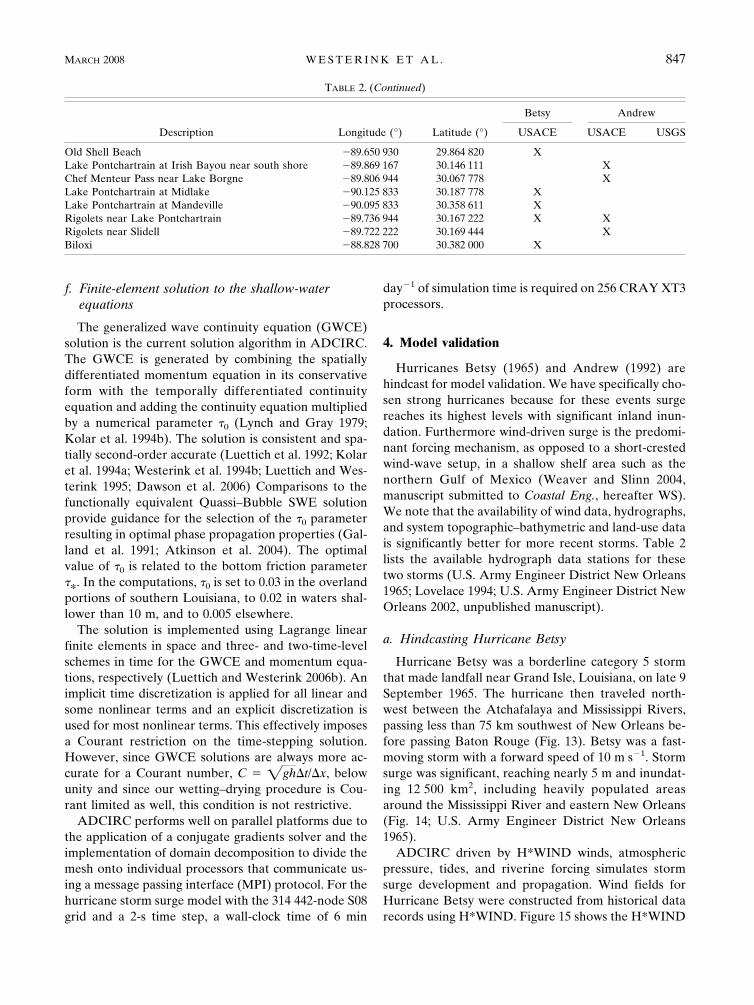
TABLE 2. List of hydrograph data locations available from the USACE and USGS for Hurricanes Betsy and Andrew. USACE datafor Betsy are from U.S. Army Engineer District, New Orleans (1965), USACE data for Andrew were obtained from the U.S. ArmyEngineer District, New Orleans (2002, personal communication), and USGS data for Andrew are available from Lovelace (1994).

Description Longitude (°) Latitude (°)

Betsy Andrew

USACE USACE USGS

East Fork tributary near Cameron �93.332 778 29.828 333 XNorth Calcasieu Lake near Hackberry �93.299 444 30.031 667 XFreshwater Bayou Lock South �92.305 833 29.552 500 XFreshwater Canal above Beef Ridge �92.305 278 29.555 000 XICW at Leland Bowman Lock East �92.194 444 29.783 333 XCypremort Point �91.881 667 29.713 889 XLuke’s Landing �91.543 056 29.596 667 XMud Lake �91.609 400 29.755 800 XWax Lake outlet at Calumet �91.372 778 29.697 778 XWax Lake outlet at Calumet �91.368 611 29.702 500 XBayou Teche at West Calumet Floodgate �91.375 278 29.703 611 XSix Mile Lake near Verdunville �91.393 056 29.763 611 XWax Lake East Control Structure South �91.322 778 29.640 833 XEugene Island �91.381 667 29.379 167 XRound Bayou at Deer Island �91.262 778 29.474 444 XLower Atchafalaya River below Sweet Bay Lake near Morgan City �91.244 722 29.551 667 XBayou Boeuf Lock East on ICW �91.173 611 29.683 056 XLower Atchafalaya River at Morgan City �91.210 833 29.694 444 X XGrand Lake at Charenton �91.523 889 29.905 556 XChicot Pass at West Fork Chicot Pass �91.485 556 30.060 833 XBayou La Rompe at Lake Long �91.588 333 30.224 722 XBlind Tesas Cut below Upper Grand River �91.565 000 30.240 556 XBayou Beouf at Amelia �91.097 222 29.668 333 XHouma Navigation Canal at Dulac �90.729 722 29.385 000 XDulac �90.715 370 29.389 640 XLake tributary to Lake Boudreaux SW of Chauvin �90.621 667 29.426 944 XBayou Lafourche at Leeville �90.208 889 29.247 778 XBayou Blue near Catfish Lake �90.346 944 29.391 944 XGrand Bayou tributary west of Galliano �90.422 222 29.455 556 XBarataria Pass east of Grand Isle �89.941 667 29.275 278 X XBarataria Bay north of Grand Isle �89.946 944 29.419 722 XTennessee Canal near cutoff �90.195 833 29.455 556 XLittle Lake near cutoff �90.184 167 29.515 556 XBayou Barataria at Lafitte �90.110 000 29.668 333 X XLareussite Canal near Naomi �90.016 667 29.691 667 XBayou Barataria at Barataria �90.132 222 29.741 389 XAlgiers Lock �89.974 444 29.911 944 XSouth Pass �89.133 300 29.000 000 XMississippi River at Empire �89.595 833 29.390 278 XMississippi River at Port Sulphur �89.689 444 29.477 222 XMississippi River at Pointe-a-la-Hache �89.796 944 29.571 111 X XMississippi River at Alliance �89.969 722 29.685 278 XMississippi River at Algiers Lock �89.968 990 29.920 799 XMississippi River at Chalmette �90.003 333 29.945 000 X XMississippi River at New Orleans (Carrollton) �90.136 111 29.934 722 XMississippi River at Bonnet Carre �90.443 056 29.998 611 XMississippi River at Baton Rouge �91.202 778 30.425 000 XCalifornia Bay near Sunrise Point northeast of Naim �89.568 056 29.485 556 XNorth California Bay near Pointe-a-la-Hache �89.583 333 29.516 667 XNE Bay Gardene near Pointe-a-la-Hache �89.666 667 29.600 000 XBlack Bay near Snake Island near Pointe-al-la-Hache �89.566 667 29.633 333 XLake Pontchartrain at West End �90.115 556 30.021 667 XIHNC near Seabrook Bridge �90.032 778 30.029 167 XMRGO at Paris Rd. �89.934 722 30.006 667 X XBayou Bienvenue at floodgate east �89.915 278 29.997 778 XMRGO at Shell Beach �89.683 333 29.850 000 X


f. Finite-element solution to the shallow-waterequations

The generalized wave continuity equation (GWCE)solution is the current solution algorithm in ADCIRC.The GWCE is generated by combining the spatiallydifferentiated momentum equation in its conservativeform with the temporally differentiated continuityequation and adding the continuity equation multipliedby a numerical parameter �0 (Lynch and Gray 1979;Kolar et al. 1994b). The solution is consistent and spa-tially second-order accurate (Luettich et al. 1992; Kolaret al. 1994a; Westerink et al. 1994b; Luettich and Wes-terink 1995; Dawson et al. 2006) Comparisons to thefunctionally equivalent Quassi–Bubble SWE solutionprovide guidance for the selection of the �0 parameterresulting in optimal phase propagation properties (Gal-land et al. 1991; Atkinson et al. 2004). The optimalvalue of �0 is related to the bottom friction parameter�*. In the computations, �0 is set to 0.03 in the overlandportions of southern Louisiana, to 0.02 in waters shal-lower than 10 m, and to 0.005 elsewhere.

The solution is implemented using Lagrange linearfinite elements in space and three- and two-time-levelschemes in time for the GWCE and momentum equa-tions, respectively (Luettich and Westerink 2006b). Animplicit time discretization is applied for all linear andsome nonlinear terms and an explicit discretization isused for most nonlinear terms. This effectively imposesa Courant restriction on the time-stepping solution.However, since GWCE solutions are always more ac-curate for a Courant number, C � �gh�t/�x, belowunity and since our wetting–drying procedure is Cou-rant limited as well, this condition is not restrictive.

ADCIRC performs well on parallel platforms due tothe application of a conjugate gradients solver and theimplementation of domain decomposition to divide themesh onto individual processors that communicate us-ing a message passing interface (MPI) protocol. For thehurricane storm surge model with the 314 442-node S08grid and a 2-s time step, a wall-clock time of 6 min

day�1 of simulation time is required on 256 CRAY XT3processors.

4. Model validation

Hurricanes Betsy (1965) and Andrew (1992) arehindcast for model validation. We have specifically cho-sen strong hurricanes because for these events surgereaches its highest levels with significant inland inun-dation. Furthermore wind-driven surge is the predomi-nant forcing mechanism, as opposed to a short-crestedwind-wave setup, in a shallow shelf area such as thenorthern Gulf of Mexico (Weaver and Slinn 2004,manuscript submitted to Coastal Eng., hereafter WS).We note that the availability of wind data, hydrographs,and system topographic–bathymetric and land-use datais significantly better for more recent storms. Table 2lists the available hydrograph data stations for thesetwo storms (U.S. Army Engineer District New Orleans1965; Lovelace 1994; U.S. Army Engineer District NewOrleans 2002, unpublished manuscript).

a. Hindcasting Hurricane Betsy

Hurricane Betsy was a borderline category 5 stormthat made landfall near Grand Isle, Louisiana, on late 9September 1965. The hurricane then traveled north-west between the Atchafalaya and Mississippi Rivers,passing less than 75 km southwest of New Orleans be-fore passing Baton Rouge (Fig. 13). Betsy was a fast-moving storm with a forward speed of 10 m s�1. Stormsurge was significant, reaching nearly 5 m and inundat-ing 12 500 km2, including heavily populated areasaround the Mississippi River and eastern New Orleans(Fig. 14; U.S. Army Engineer District New Orleans1965).

ADCIRC driven by H*WIND winds, atmosphericpressure, tides, and riverine forcing simulates stormsurge development and propagation. Wind fields forHurricane Betsy were constructed from historical datarecords using H*WIND. Figure 15 shows the H*WIND

TABLE 2. (Continued)

Description Longitude (°) Latitude (°)

Betsy Andrew

USACE USACE USGS

Old Shell Beach �89.650 930 29.864 820 XLake Pontchartrain at Irish Bayou near south shore �89.869 167 30.146 111 XChef Menteur Pass near Lake Borgne �89.806 944 30.067 778 XLake Pontchartrain at Midlake �90.125 833 30.187 778 XLake Pontchartrain at Mandeville �90.095 833 30.358 611 XRigolets near Lake Pontchartrain �89.736 944 30.167 222 X XRigolets near Slidell �89.722 222 30.169 444 XBiloxi �88.828 700 30.382 000 X


maximum marine wind velocity adjusted to 10-min-averaged winds. We note some chatter to the west ofthe track, which is a result of the interpolation intervalused to produce the figure. Figure 16 shows theH*WIND maximum applied 10-min-averaged windsadjusted with the directional land-masking algorithm,the inundation algorithm, and the forested canopy fac-tor. We note that to the east of the Mississippi River,the differences between the marine and adjusted windsare due to directional roughness effects along the northshore of Lake Pontchartrain, due to forested canopiesaround Lake Maurepas and due to roughness effects inthe vicinity of English Turn. Due to the wind coming offof open water and the extensive inundation in the re-gion, the overall adjustment of the marine winds wasnot dramatic in this region. A purely local wind bound-ary layer adjustment that does not account for floodingwould in fact lead to winds in this area that are reducedmuch more than with our adjustments. To the west ofthe Mississippi River, surface roughness and canopiessubstantially alter the marine winds. The adjustedwinds are interpolated onto the ADCIRC grid. Nodalfactors and equilibrium arguments for the five astro-nomical forcing tides were computed for the startingtime of the simulation: 0000 UTC 18 August 1965. TheMississippi River was forced with a specified flow of5520 m3 s�1 and the Atchafalaya River was forced witha specified flow of 2200 m3 s�1.

Betsy winds drive Gulf waters across Breton Soundtoward the Mississippi River. There is a levee only on

the western bank of the Mississippi River for nearly thesecond half of the river below New Orleans in Plaque-mines Parish. This allows surge driven in from BretonSound to build up in the river and east of the river tomore than 4 m. The surge in the river then propagatesupstream and passes New Orleans and Baton Rouge atapproximately 3.5 m. The same regional surge east ofthe river also propagates north through Breton Soundand the marshes west of Breton Sound, and is stoppedby the Mississippi River levees at English Turn. Wateris also blown across from the Gulf into ChandeleurSound and Lake Borgne, and builds up in the funnelbetween St. Bernard Parish and New Orleans East, re-sulting in extensive inundation due to the low leveeheights in the area in 1965. Similarly, water levels ex-ceed 4 m in the southwest corner of Lake Pontchar-train, which is in line with the high storm winds comingacross the shallow lake. In addition, the high waters onthe west side of Lake Borgne coupled with the loweredwater levels in eastern Lake Pontchartrain drive flowthrough Chef Menteur Pass and the Rigolets into LakePontchartrain and raise the overall level of the lake.Finally, flooding over Grand Isle into Barataria Bayand the surrounding areas penetrates farthest inland(more than 100 km) to Lac Des Allemands and thesurrounding areas, which is just to the southwest of theNew Orleans levee system.

The modeled distribution of peak storm surgeheights throughout the event is shown for southeasternLouisiana in Fig. 17. Surge typically reaches its greatestheights against the levee structures. The MississippiRiver levees in Plaquemines Parish prevent water frompropagating from Breton Sound across into BaratariaBay and cause water levels to build up in a large area tothe southeast of New Orleans. The levee configurationalso contributes to storm surge amplification through afocusing process in this area. The river and levees makea sharp turn at the southeastern edge of New Orleans atEnglish Turn, creating a concave area that amplifiesstorm surge. The funnel-shaped region between St.Bernard Parish and New Orleans East also effectivelyamplifies surge. In the western end of Lake Pontchar-train, flow is stopped by a raised railroad and surgeexceeds 4 m. The Bonne Carre spillway region is im-pacted with some of the highest water levels. The extentof modeled flooding in Fig. 17 can be compared to thatrecorded from Hurricane Betsy by the U.S. ArmyCorps of Engineers (Fig. 14). The flooded areas com-pare well: both have widespread flooding around LakePontchartrain and Lake Maurepas, in eastern New Or-leans and areas east of the Mississippi River, and south-west of New Orleans down to the Gulf of Mexico.

Figure 18 shows the significant effect of the direc-

FIG. 13. Hurricane Betsy track data for the time that winds wereapplied in the ADCIRC simulation between 1200 UTC 8 Sep and0000 UTC 13 Sep. The position of the eye is given every 6 h.Maximum storm wind speed at each eye position is in m s�1 for10-min-averaged winds.


Fig 13 live 4/C

tional wind reduction algorithm, inundation relatedwind increases, and canopy reductions on the maximumwater levels during the storm. In general, the full ma-rine winds lead to a small reduction of the maximumsurge on the order of 5 cm as the winds come acrossopen water; they then build to an increase of 30 cm tomore than 1 m as water is pushed up against structuresand higher land. The effect of the canopies in the vi-cinity of Lake Maurepas is particularly strong with thefull marine wind leading to more significant nearshorereductions and downwind increases. We note that ourcombined wind modification algorithm can actuallylead to winds that are closer to marine winds in casessuch as the wind coming off of open water and whenoverland inundation occurs, which covers the physicalroughness elements. Since Fig. 18 only shows the maxi-mum water levels during the storm, the reduction in lowwater levels that the algorithm produces is not illus-trated.

Differences between the modeled and recorded peakstorm surges are calculated in meters at 20 stationswhere gauges recorded water levels during Betsy(Table 2). These errors are shown on the map of peakmodeled errors (Fig. 19). The data record is matched to

the modeled water level by examining 0.75 days ofrecord prior to the storm surge signal arriving to ac-count for local data differences in the source data aswell as the locally variable subsidence rates. However,this is not possible at all locations due to incompletedata records. The mean error is 0.58 m and the standarddeviation is 0.53 m. There are two obvious outliers thatare related to missing subgrid-scale features (gates orother controls) and/or vertical datum problems. Withthese two outliers removed, the mean peak surge errorfor the remaining 18 data points is reduced to 0.43 mand the standard deviation to 0.31 m.

Time series of the model response during HurricaneBetsy are compared to water-level data at the tidal andriver gauges. Hydrographs at 12 stations are plottedwith the data records and model output in Fig. 20. Themodel shows a good match to both the tidal signal andthe surge although the surge buildup prior to the peakand dieoff following the peak occur more quickly in themodel than in the observations.

b. Hindcasting Hurricane Andrew

Hurricane Andrew struck southern Louisiana nearthe mouth of the Atchafalaya River at Point Chevreuil

FIG. 14. Recorded inundation from Hurricane Betsy (from U.S. Army Engineer District, New Orleans 1965). Blue indicates waterbodies, beige indicates dry land, and yellow indicates normally dry land inundated during Hurricane Betsy.


Fig 14 live 4/C

at approximately 0730 UTC on 26 August 1992 as acategory 4 storm. The storm made landfall farther westthan Betsy but took a more northerly track, passing justto the west of Baton Rouge (Figs. 21 and 22). With aforward speed of approximately 4 m s�1, Andrewmoved slower than Betsy at landfall. The hurricaneflooded many unprotected areas around the MississippiRiver, Lake Pontchartrain, and within the Atchafalaya

River flood basin with its peak surge approaching 2.5 mjust east of the eye and 3 m in areas close to NewOrleans (Rappaport 2006).

The Hurricane Andrew wind field was reconstructedusing the PBL model, based on the storm’s track, maxi-mum wind speed, and minimum pressure. Figure 23shows the maximum 10-min-averaged marine windspeed contours from the PBL model output. Figure 24

FIG. 15. Hurricane Betsy 10-min-averaged maximum marine wind speed contours from H*WIND(m s�1) across southeastern LA.

FIG. 16. Hurricane Betsy 10-min-averaged maximum directionally reduced wind speed contours fromH*WIND (m s�1) across southeastern LA.



shows the PBL maximum applied 10-min-averagedwinds adjusted with the directional land-masking algo-rithm, the inundation algorithm, and the canopy factor.The adjusted PBL model winds are compared to datarecorded during Hurricane Andrew to validate thewind model. The recorded data are taken at 12 meteo-rological stations located at airfields, along the coast,and at offshore buoys (Fig. 22, Table 3). Comparisons

between the modeled and recorded wind data are madefor wind speed and direction from 25 through 28 Au-gust in Figs. 25 and 26. Modeled and measured windsshow very good agreement, although small-scale localfluctuations seen in the data record are not reproducedin the modeled winds. We note in Fig. 22 that the com-parison anemometers are distributed along the stormtrack as well as away from the most intense portion of

FIG. 18. Difference in Hurricane Betsy modeled peak storm surge elevation (m) in southeastern LAwhen modeled with marine winds and with directionally reduced winds. Levee structures are shown asbrown lines.

FIG. 17. Hurricane Betsy modeled peak storm surge elevation (m) relative to NGVD29 in southeasternLA computed with directionally reduced winds. Levee structures are shown as brown lines.



the storm and are located in open water, inland, andnear shore. As such, they indicate that the storm isregionally well captured and that the wind reductionalgorithms work well. Nodal factors and equilibriumarguments for the five astronomical forcing tides werecomputed for the starting time of the simulation: 0000UTC 4 August 1992. The Mississippi River was forcedwith a specified flow of 11200 m3 s�1 and the Atchafa-laya River was forced with a specified flow of 4850m3 s�1.

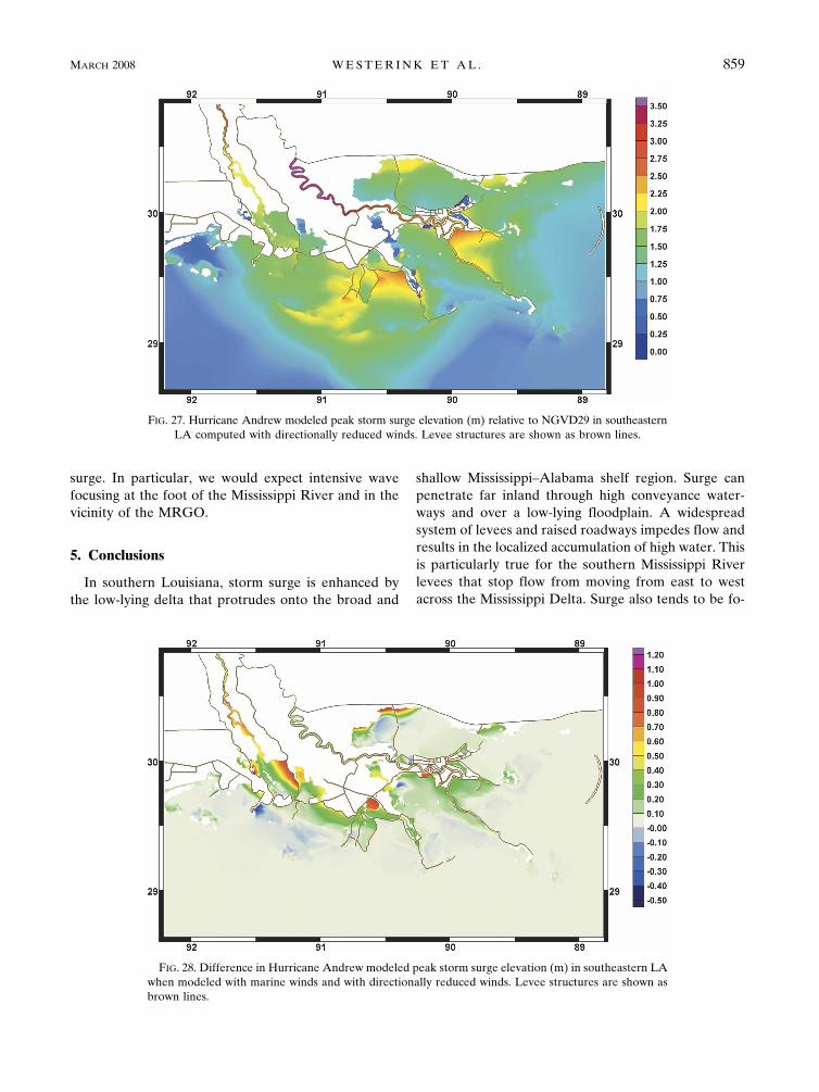
As Andrew first approaches Louisiana, early highsurge levels are observed on the eastern side of theMississippi River levees and Breton Sound, and wateris driven into Lake Borgne and Lake Pontchartrain. Asthe eye makes landfall, it drives surge well above 2 m onits right side while dropping water levels on its left side.The Mississippi River east bank levee system focusesthe surge to a peak approaching 3 m at English Turn, aswith Betsy. Flooding from Barataria Bay inundatesmost of the area south of New Orleans and high wateris driven into Timbalier and Terrebonne Bays. Themain volume of surge inundates most areas south of theGIWW across southern Louisiana. Depths range from2.5 m near Larose to approximately 1.75 m of surge upthe Atchafalaya River. High water levels in Lake Pont-chartrain are driven by Andrew’s winds to flood muchof the northwestern shore. Maximum storm surge con-tours across southeastern Louisiana are shown in Fig.27. The surge is highest in areas where the surge buildsup against the topographic contours or levee systems.

Figure 28 shows the effects of the directional wind re-duction algorithm, wind increases with inundation, andwind reductions due to canopies on the maximum waterlevels during the storm. Again, the full marine windsresult in a small reduction of the maximum surge on theorder of 5 cm as the winds come across open water, andstage level increases of approximately 30 cm to 1 m areseen as water is pushed up against structures and higherland.

The error in the modeled peak storm surge height iscalculated by determining its difference from the re-corded maximum surge at 51 gauge stations throughoutsouthern Louisiana (listed in Table 2). These errors areshown with the peak modeled surge in Fig. 29. Prestormwater-level differences between the model and the datarecord are used to adjust peak surge differences in or-der to account for vertical datum shifts and local sub-sidence at individual stations. The mean error in thepeak storm surge height is 0.29 m and the standarddeviation is 0.28 m. There were two clear outliers due tothe errors in the data sources as determined by a com-parison to the model output. With these two outliersremoved, the mean peak surge error for the remaining49 stations is 0.27 m and the standard deviation 0.23 m.

Time series of water-level heights from the modelduring Hurricane Andrew are compared to water-leveldata from tidal and river gauges. These hydrographsshow the progression of the tidal and surge response asthe storm evolves. Twelve stations were chosen fromthe data available during Andrew, and the hydrographs

FIG. 19. Hurricane Betsy modeled peak storm surge elevation errors (m) in southeastern LA com-pared with measured data at 20 stations listed in Table 2. Positive error values indicate model overpre-diction and negative values indicate underprediction. Levee structures are shown as brown lines.


Fig 19 live 4/C

FIG. 20. Hydrographs of modeled (solid line) and recorded (dashed line) water surface elevation (m) relative to NGVD29 duringHurricane Betsy. Dry model response and unavailable data are assigned a value of �99 999.


FIG. 21. Hurricane Andrew track data for the time that winds were applied in the ADCIRC simulationbetween 0000 UTC 22 Aug and 0000 UTC 28 Aug. The position of the eye is given every 6 h. Maximumstorm wind speed at each eye position is in m s�1 for 10-min-averaged winds.

FIG. 22. Detail for Hurricane Andrew track data across the northern Gulf of Mexico. The position ofthe eye is given every 6 h. Maximum storm wind speed at each eye position is in m s�1 for 10-min-averaged winds. Anemometer station numbers listed in Table 3 are indicated.



from the data records and model output are shown inFig. 30. With the exception of prestorm differences inwater levels due to vertical datum errors, the modelclosely matches the tidal signal and storm surge re-sponse.

c. Assessment of model skill

Peak modeled storm surge height is comparedagainst the peak recorded storm surge height for Betsy

and Andrew in Fig. 31 after adjusting for vertical datumand local subsidence based on prestorm water levelsand excluding the four outliers. The slope of the regres-sion line is 0.91, indicating that the model is underpredict-ing surge by approximately 9%. The correlation coeffi-cient, R2, is 0.804. Examining Betsy and Andrew individu-ally shows that Andrew’s surge more closely matchesthe recorded surge (slope equals 0.924 versus 0.899).

In Fig. 31, the station data points are divided into five

FIG. 24. Hurricane Andrew 10-min-averaged maximum directionally reduced wind speed contoursfrom PBL (m s�1) across southeastern LA.

FIG. 23. Hurricane Andrew 10-min-averaged maximum marine wind speed contours from PBL(m s�1) across southeastern LA.



regions that are demarcated by the two main rivers inLouisiana, as river levee systems generally keep thesurge from propagating between these regions. Gridresolution is typically poorest in the west, and is best inthe New Orleans region and around the Mississippi andAtchafalaya Rivers. Results within the Atchafalayaand, especially, Mississippi Rivers have less varianceand tend to be more accurate than in other areas. Thisindicates that the model is correctly simulating both thesurge entering the rivers and surge–tide–current inter-action. The model appears to be generally less accuratein the region between the Atchafalaya River basin andthe Mississippi River. This area has a significant stormsurge response but is not as highly resolved by themodel grid nor are the bathymetric and topographicdata as complete or reliable in these areas. In addition,there are local features such as levee systems and raisedroads that are not represented in the model grid. Ex-amination of the model response east of the MississippiRiver, where mesh resolution is highest and most accu-rate, shows that the model tends to underpredict stormsurge, suggesting the model is not incorporating all ofthe processes contributing to storm surge generation.

To examine the overall characteristics of the model,the differences between the peak and modeled stormsurges for Betsy and Andrew at all stations (with theexception of the outliers) are sorted into 0.10-m incre-ments and plotted in a histogram in Fig. 32. While themost frequently occurring errors are between �0.1 and0.1 m, it is clear that the model tends to generally un-derpredict the storm surge. Analysis of the differencesbetween the modeled and recorded surge height showsa mean error of �0.15 m, an absolute mean error of0.30 m, and a standard deviation of 0.37 m.

The most significant factor influencing local modelskill is adequate resolution of the hydrodynamic and

geographic features. It is likely that the stations with apoor match between the model and observations havesurge controlled by features such as local channels,levees, or floodgates that have not been resolved in themodel grid. We believe that this is particularly true forthe region between the Atchafalaya River basin and theMississippi River, where we know that the model grid ismissing many such small-scale features. In the northernportion of this region, the model surge is too high be-cause there is too much conveyance of water throughthe areas closer to the open ocean. In the southernportion of this region, there is a systematic underrep-resentation of storm surge elevation that may be partlydue to the lack of levees and raised roads that cause thesurge to pile up in these areas.

Wind waves influence surge height with wind-waveradiation stress, modifying bottom friction, and chang-ing sea surface roughness. Modeling studies haveshown that the surge increase due to the wind-wavesetup can be proportionally more significant for weakerwinds and steep bathymetric profiles (WS). Althoughwind waves tend to be proportionately less importantfor strong storms on wide shallow shelves, they do in-fluence the total surge away from the center of thestorm, affect the time of arrival of the peak surge, andtend to reduce drawdown. Wind waves reach shoreprior to the peak surge driven by the strongest hurri-cane winds, so the combined wind and wind-wave surgebuilds up earlier than does the solely wind-driven surge.Furthermore, drawdown caused by winds coming fromshore tends to be reduced by waves that are still cominginto shore. These factors are consistent with the com-parisons of model and observed hydrographs and peaksurge that show that the model produces shorter-duration surges and that the percentage of peak surgeunderprediction is greater for modest levels of storm

TABLE 3. Wind data records during Hurricane Andrew from NOAA Coastal-Marine Automated Network (C-MAN) stations,NOAA National Data Buoy Center (NDBC) buoys (information online at http://www.ndbc.noaa.gov), and NOAA National ClimaticData Center (NCDC) stations (information online at http://www.ncdc.noaa.gov/oa/climate/stationlocator.html).

Name Source description Lat Lon

333 km south of Southwest Pass, LA NDBC Buoy 42001 25°54�00�N 89°40�00�W27.88°N, 90.90°W C-MAN Bullwinkle Block (industry platform) 27°52�48�N 90°54�00�WLake Charles NCDC Lake Charles Regional Airport 30°07�N 93°14�WHouma NCDC Houma Terrebonne Airport 29°33�N 90°40�WSalt Point NCDC Salt Point, LA 29°34�N 91°32�WGrand Isle C-MAN GDIL1 29°16�00�N 89°57�24�WSouthwest Pass C-MAN BURL1 28°54�18�N 89°25�42�WNew Orleans International Airport NCDC New Orleans International Airport 29°59�N 90°15�WNew Orleans Lakefront NCDC New Orleans Lakefront Airport 30°03�N 90°02�WKeesler AFB NCDC Biloxi Keesler Air Force Base 30°25�N 88°55�W40 km SSE of Biloxi NDBC Buoy 42007 30°05�25�N 88°46�07�WDauphin Island C-MAN DPIA1 30°14�54�N 88°04�24�W


FIG. 25. Modeled (solid line) and recorded (dashed line) wind speed during Hurricane Andrew at the anemometer stations listed inTable 3.


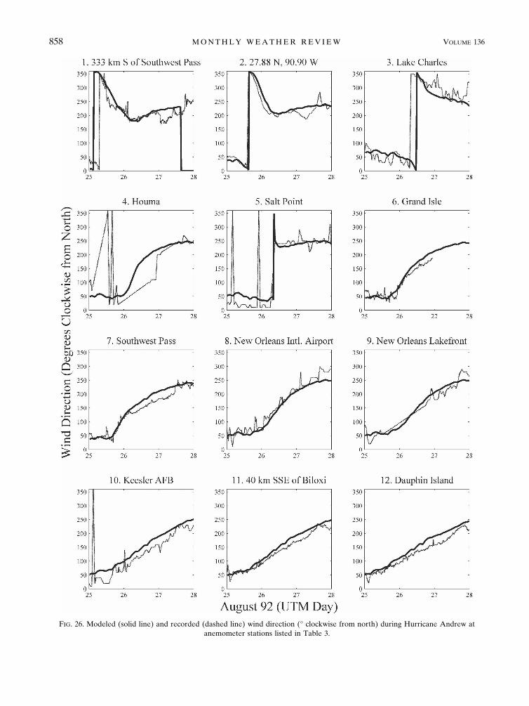
FIG. 26. Modeled (solid line) and recorded (dashed line) wind direction (° clockwise from north) during Hurricane Andrew atanemometer stations listed in Table 3.


surge. In particular, we would expect intensive wavefocusing at the foot of the Mississippi River and in thevicinity of the MRGO.

5. Conclusions

In southern Louisiana, storm surge is enhanced bythe low-lying delta that protrudes onto the broad and

shallow Mississippi–Alabama shelf region. Surge canpenetrate far inland through high conveyance water-ways and over a low-lying floodplain. A widespreadsystem of levees and raised roadways impedes flow andresults in the localized accumulation of high water. Thisis particularly true for the southern Mississippi Riverlevees that stop flow from moving from east to westacross the Mississippi Delta. Surge also tends to be fo-

FIG. 28. Difference in Hurricane Andrew modeled peak storm surge elevation (m) in southeastern LAwhen modeled with marine winds and with directionally reduced winds. Levee structures are shown asbrown lines.

FIG. 27. Hurricane Andrew modeled peak storm surge elevation (m) relative to NGVD29 in southeasternLA computed with directionally reduced winds. Levee structures are shown as brown lines.



cused in lateral convergences defined by raised fea-tures, such as at English Turn and the funnel betweenSt. Bernard Parish and New Orleans East.

A hydrodynamic model has been developed that re-solves the features important to storm surge propaga-tion on a local scale while providing accurate modelforcing and parameterization of physical processes. TheADCIRC model uses unstructured grids that providethe resolution of the hydrodynamic and geographic fea-tures governing storm surge propagation on a local ba-sis. The domain incorporates the western North Atlan-tic Ocean, the Gulf of Mexico, and the Caribbean Sea,in order to provide accurate forcing for tides and hur-ricanes at the open-ocean boundary and inherently cap-tures all significant processes as the storm tracks fromthe ocean through the resonant Gulf and Caribbeanbasins and onto the shelf. Within the overland regions,extensive levee systems and raised roadways are incor-porated and all significant channels and waterways arerepresented.

ADCIRC is validated by hindcasting HurricanesBetsy and Andrew. Modeled water surface elevationwas recorded at gauge station locations throughoutsouthern Louisiana for comparison to hydrographicdata. These comparisons show the ability of the modelto accurately simulate storm surge across Louisiana; themean peak surge error for Betsy is 0.43 m and for An-drew it is 0.27 m. Comparisons of the modeled to ob-served peak storm surges show that the model on av-erage lies approximately 10% below the observations.

Despite the well-resolved computational mesh, accu-rate boundary condition specification and meteorologi-cal forcing, and physically realistic parameterizations ofsurface and subgrid-scale effects, there are areas wherethe model over- or underpredicts the observed stormsurge. We believe there are three areas where it wouldbe helpful to include additional processes contributingto storm surge generation into the model.

First, model errors appear to be associated with re-gions (e.g., between the Atchafalaya and MississippiRivers) where bathymetric and topographic data aresparse and where raised features have not been in-cluded in the model grid. Recent lidar-based topo-graphic surveys can be used to better define the topog-raphy and the raised features that tend to be impedi-ments to storm surge propagation. In addition, verticaldatum definitions should be improved in both the systemdefinition as well as in the observational data allowingfor a better representation of the system while also per-mitting direct comparisons to high water mark data.

Second, the hydrodynamic model is lacking the ad-ditional momentum transfer and setup to the stormsurge due to short-crested wind waves. This effect be-comes relatively more important away from the centerof the storm and may contribute a significant portion ofthe surge height at lower wind conditions. These wind-wave effects are also likely to contribute to water-levelsetup prior to and following the arrival of peak winds,which are times when our model tends to underpredictwater levels. We are in the process of coupling ADCIRC

FIG. 29. Hurricane Andrew modeled peak storm surge elevation errors (m) in southeastern LAcompared to measured data at 51 stations listed in Table 2. Positive error values indicate model over-prediction and negative values indicate underprediction. Levee structures are shown as brown lines.


Fig 29 live 4/C

FIG. 30. Hydrographs of modeled (solid line) and recorded (dashed line) water surface elevation (m) relative to NGVD29 duringHurricane Andrew.


to several wind-wave models to further assess the sig-nificance of this forcing.

Third, the application of standard wind drag coeffi-cient relationships may not fully characterize the sea

surface roughness and resulting shear stress in a hurri-cane. There is evidence that a drag coefficient that issolely dependent upon wind speed does not fully de-scribe the actual sea state conditions. The inclusion of a

FIG. 31. Comparison of recorded vs modeled peak storm surge elevation (m) fromstation data listed in Table 2. Betsy results appear in blue and Andrew results in red.

FIG. 32. Histogram of recorded minus modeled peak surge (m) using 67 observations ofpeak water levels during Hurricanes Betsy and Andrew.


Fig 31 live 4/C

wind-wave model will better define the sea surfaceroughness and will allow for incorporation of drag co-efficient relationships that are dependent upon thewind-wave conditions.

Acknowledgments. We thank Robert G. Dean of theUniversity of Florida at Gainesville and Robert O.Reid of Texas A&M University for their insight anddiligent review of our work as part of an external re-view board for the USACE-MVN. In addition, wethank Harley Winer, Jay Combe, Jay Ratcliff, and MaikFlanagin of the USACE-MVN for significant input.

Funding for the S08 model was provided by theUSACE-MVN. In particular, we thank Al Naomi forhis strong support of this effort. Funding for ADCIRCcode development has been provided by the U.S. ArmyEngineer Research and Development Center, the Na-tional Science Foundation, the Office of Naval Re-search, the U.S. Naval Research Laboratory, the U.S.Army Research Office, and the Texas Water Develop-ment Board.

REFERENCES

Atkinson, J. H., J. J. Westerink, and J. M. Hervouet, 2004: Simi-larities between the wave equation and the quasi-bubble so-lutions to the shallow water equations. Int. J. Numer. Meth-ods Fluids, 45, 689–714.

Blain, C. A., J. J. Westerink, and R. A. Luettich, 1994: The influ-ence of domain size on the response characteristics of a hur-ricane storm surge model. J. Geophys. Res., 99 (C9), 18 467–18 479.

——, ——, and ——, 1998: Grid convergence studies for the pre-diction of hurricane storm surge. Int. J. Numer. Methods Flu-ids, 26, 369–401.

Cardone, V. J., C. V. Greenwood, and J. A. Greenwood, 1992:Unified program for the specification of hurricane boundarylayer winds over surfaces of specified roughness. ContractRep. CERC-92-1, U.S. Army Corps of Engineers, 85 pp. � 3appendixes. [Available from ERDC Vicksburg (WES), U.S.Army Engineer Waterways Experiment Station (WES),ATTN: ERDC-ITL-K, 3909 Halls Ferry Rd., Vicksburg, MS39180-6199.]

——, A. T. Cox, J. A. Greenwood, and E. F. Thompson, 1994:Upgrade of the tropical cyclone surface wind field model.Miscellaneous Paper CERC-94-14, U.S. Army Corps of En-gineers, 27 pp � 4 appendixes. [Available from ERDC Vicks-burg (WES), U.S. Army Engineer Waterways ExperimentStation (WES), ATTN: ERDC-ITL-K, 3909 Halls Ferry Rd.,Vicksburg, MS 39180-6199.]

Charnock, H., 1955: Wind stress on a water surface. Quart. J. Roy.Meteor. Soc., 81, 639–640.

Coleman, J. M., H. H. Roberts, and G. W. Stone, 1998: MississippiRiver delta, an overview. J. Coastal Res., 14, 698–716.

Dawson, C., J. J. Westerink, J. C. Feyen, and D. Pothina, 2006:Continuous, discontinuous and coupled discontinuous–continuous Galerkin finite element methods for the shallowwater equations. Int. J. Numer. Methods Fluids, 52, 63–88.

Dietrich, J. C., R. L. Kolar, and J. J. Westerink, 2006: Refine-

ments in continuous Galerkin wetting and drying algorithms.Proc. Ninth Int. Conf. on Estuarine and Coastal Modeling,Charleston, SC, ASCE, 637–656.

Federal Emergency Management Agency, 2006: Multi-hazard lossestimation methodology hurricane model. Dept. of Home-land Security Tech. Manual HAZUS MH MR3, 598 pp.[Available online at http://www.fema.gov/library/viewRecord.do?id�3034.]

Feyen, J. C., J. H. Atkinson, and J. J. Westerink, 2002: GWCE-based shallow water equation simulations of the Lake Pont-chartrain–Lake Borgne tidal system. Computational Methodsin Water Resources, Vol. II, S. M. Hassanizadeh et al., Eds.,Developments in Water Science, Vol. 47, Elsevier, 1581–1588.

Flather, R. A., and K. P. Hubbert, 1990: Tide and surge modelsfor shallow water—Morecambe Bay revisited. Modeling Ma-rine Systems, Vol. I, A. M. Davies, Ed., CRC Press, 135–166.

Galland, J., N. Goutal, and J. Hervouet, 1991: A new numericalmodel for solving the shallow water equations. Adv. WaterRes., 14, 138–148.

Garratt, J. R., 1977: Review of drag coefficients over oceans andcontinents. Mon. Wea. Rev., 105, 915–929.

Hagen, S. C., J. J. Westerink, and R. L. Kolar, 2000: Finite ele-ment grids based on a localized truncation error analysis. Int.J. Numer. Methods Fluids, 32, 241–261.

——, ——, ——, and O. Horstmann, 2001: Two dimensional un-structured mesh generation for tidal models. Int. J. Numer.Methods Fluids, 35, 669–686.

Holland, G., 1980: An analytic model of the wind and pressureprofiles in hurricanes. Mon. Wea. Rev., 108, 1212–1218.

Hsu, S., 1988: Coastal Meteorology. Academic Press, 260 pp.Kolar, R. L., W. G. Gray, J. J. Westerink, and R. A. Luettich,

1994a: Shallow water modeling in spherical coordinates:Equation formulation, numerical implementation and appli-cation. J. Hydraul. Res., 32, 3–24.

——, J. J. Westerink, M. E. Cantekin, and C. A. Blain, 1994b:Aspects of nonlinear simulations using shallow water modelsbased on the wave continuity equation. Comput. Fluids, 23,523–538.

Leendertse, J. J., 1987: Aspects of SIMSYS2D: A system for two-dimensional flow computation. Rand Corporation Rep.R-3572-USGS, Santa Monica, CA, 80 pp.

Le Provost, C., F. Lyard, J. Molines, M. Genco, and F. Rabilloud,1998: A hydrodynamic ocean tide model improved by assimi-lating a satellite altimeter-derived data set. J. Geophys. Res.,103, 5513–5529.

Lovelace, J. K., 1994: Storm-tide elevations produced by Hurri-cane Andrew along the Louisiana coast, August 25–27, 1992.U.S. Geological Survey Open File Rep. 94-371, Baton Rouge,LA, 45 pp.

Luettich, R. A., and J. J. Westerink, 1995: Continental shelf scaleconvergence studies with a barotropic model. QuantitativeSkill Assessment for Coastal Ocean Models, D. R. Lynch andA. M. Davies, Eds., Coastal and Estuarine Studies Series, No.47, Amer. Geophys. Union, 349–371.

——, and ——, 1999: Elemental wetting and drying in the AD-CIRC hydrodynamic model: Upgrades and documentationfor ADCIRC version 34.XX. Contractors Rep., U.S. ArmyCorps of Engineers, 8 pp. [Available from ERDC Vicksburg(WES), U.S. Army Engineer Waterways Experiment Station(WES), ATTN: ERDC-ITL-K, 3909 Halls Ferry Road,Vicksburg, MS 39180-6199.]

——, and ——, 2003: Combined discharge and radiation bound-


ary condition in the ADCIRC hydrodynamic model: Theoryand documentation. Contractors’ Rep., U.S. Army Corps ofEngineers New Orleans District, 16 pp. [Available from U.S.Army Engineer Corps of Engineers, New Orleans, ATTN:CEMVN-IM-SM Library, P.O. Box 60267, New Orleans, LA70160-0267.]

——, and ——, cited 2006a: ADCIRC: A parallel advanced cir-culation model for oceanic, coastal and estuarine waters; us-ers manual for version 45.08. [Available online at http://adcirc.org/document/ADCIRC_title_page.html.]

——, and ——, cited 2006b: Formulation and numerical imple-mentation of the 2D/3D ADCIRC finite element model, ver-sion 44.XX. [Available online at http://adcirc.org/adcirc_theory_2004_12_08.pdf.]

——, ——, and N. W. Scheffner, 1992: ADCIRC: An advancedthree-dimensional circulation model for shelves, coasts andestuaries, Report 1: Theory and methodology of ADCIRC-2DDI and ADCIRC-3DL. Tech. Rep. DRP-92-6, U.S. ArmyCorps of Engineers, 137 pp. [Available from ERDC Vicks-burg (WES), U.S. Army Engineer Waterways ExperimentStation (WES), ATTN: ERDC-ITL-K, 3909 Halls Ferry Rd.,Vicksburg, MS 39180-6199.]

Lynch, D. R., and W. G. Gray, 1979: A wave equation model forfinite element tidal computations. Comput. Fluids, 7, 207–228.

Mukai, A., J. J. Westerink, R. Luettich Jr., and D. Mark, 2002:Eastcoast 2001: A tidal constituent database for the westernNorth Atlantic, Gulf of Mexico, and Caribbean Sea. Tech.Rep. ERDC/CHL TR-02-24, U.S. Army Corps of Engineers,25 pp. [Available from ERDC Vicksburg (WES), U.S. ArmyEngineer Waterways Experiment Station (WES), ATTN:ERDC-ITL-K, 3909 Halls Ferry Rd., Vicksburg, MS 39180-6199.]

National Geophysical Data Center, 1998: Geophysical Data Sys-tem for Hydrographic Survey Data. National Ocean ServiceHydrographic Survey Data, National Geophysical Data Cen-ter, Boulder CO, 2 CD-ROMs.

——, cited 2006: ETOPO5 technical report. National Oceanic andAtmospheric Administration. [Available online at http://www.ngdc.noaa.gov/mgg/global/etopo5.HTML.]

National Wetlands Research Center, cited 2006: Land cover clas-sification for the Louisiana GAP analysis. United States Geo-logical Survey Tech. Rep. [Available online at http://sdms.cr.usgs.gov/gap/gap2.html.]

Powell, M., and S. Houston, 1996: Hurricane Andrew’s landfall insouth Florida. Part II: Surface wind fields and potential real-time applications. Wea. Forecasting, 11, 329–349.

——, ——, and T. Reinhold, 1996: Hurricane Andrew’s landfall insouth Florida. Part I: Standardizing measurements for docu-mentation of surface wind fields. Wea. Forecasting, 11, 304–328.

——, ——, L. Amat, and N. Morrisseau-Leroy, 1998: The HRD

real-time hurricane wind analysis system. J. Wind Eng. In-dust. Aerodyn., 77–78, 53–64.

Rappaport, E., 2006: Preliminary report: Hurricane Andrew, 16–28 August 1992; updated 10 December 1993. National Oce-anic and Atmospheric Administration/National HurricaneCenter. [Available online at http://www.nhc.noaa.gov/1992andrew.html.]

Reid, R. O., and R. Whitaker, 1976: Wind-driven flow of waterinfluenced by a canopy. J. Waterways, Harbors, Coastal Eng.Div., 102, 61–77.

Shinkle, K. D., and R. K. Dokka, 2004: Rates of vertical displace-ment at benchmarks in the Lower Mississippi Valley and thenorthern Gulf coast. NOAA Tech. Rep. NOS/NGS 50, 135pp.

Simiu, E., and R. Scanlan, 1986: Wind Effects on Structures. WileyInterscience, 604 pp.

Thompson, E. F., and V. J. Cardone, 1996: Practical modeling ofhurricane surface wind fields. J. Waterways Port, CoastalEng., 122, 195–205.

U.S. Army Engineer District New Orleans, 1965: Report on Hur-ricane Betsy, 8–11 September 1965 in the U.S. Army Engi-neer District, New Orleans. U.S. Army Corps of EngineersNew Orleans District, Tech. Rep., 48 pp. [Available fromU.S. Army Engineer Corps of Engineers, New Orleans,ATTN: CEMVN-IM-SM Library, P.O. Box 60267, New Or-leans, LA 70160-0267.]

U.S. Geological Survey, cited 2006: National Elevation Dataset.EROS Data Center, Sioux Falls, SD. [Available online athttp://ned.usgs.gov.]

Vogelmann, J. E., S. M. Howard, L. Yang, C. R. Larson, B. K.Wylie, and N. Van Driel, 2001: Completion of the 1990s Na-tional Land Cover Data Set for the conterminous UnitedStates from Landsat Thematic Mapper data and ancillarydata sources. Photogramm. Eng. Remote Sens., 67, 650–652.

Westerink, J. J., R. A. Luettich, A. M. Baptista, N. W. Scheffner,and P. Farrar, 1992: Tide and storm surge predictions using afinite element model. J. Hydraul. Eng., 118, 1373–1390.

——, ——, and J. C. Muccino, 1994a: Modeling tides in the west-ern North Atlantic using unstructured graded grids. Tellus,46A, 178–199.

——, ——, J. K. Wu, and R. L. Kolar, 1994b: The influence ofnormal flow boundary conditions on spurious modes in finiteelement solutions to the shallow water equations. Int. J. Nu-mer. Methods Fluids, 18, 1021–1060.

——, ——, and A. Militello, 2001: Leaky internal-barrier normal-flow boundaries in the ADCIRC Coastal HydrodynamicsCode. Coastal and Hydraulic Engineering Tech. Note IV-32,U.S. Army Corps of Engineers, 26 pp. [Available online athttp://cirp.wes.army.mil/cirp/cetns/chetn-iv32.pdf or fromERDC Vicksburg (WES), U.S. Army Engineer WaterwaysExperiment Station (WES), ATTN: ERDC-ITL-K, 3909Halls Ferry Rd., Vicksburg, MS 39180-6199.]


A Basin- to Channel-Scale Unstructured Grid Hurricane ...

Documents

Transcript of A Basin- to Channel-Scale Unstructured Grid Hurricane ...