C o m m u n i t y E x p e r i e n c e D i s t i l l e d

Develop key skills and techniques with R to create and customize data mining algorithms

Learning Data Mining with RB

ater Makhabel

Learning Data Mining with R

Being able to deal with the array of problems that you may encounter during complex statistical projects can be diffi cult. If you have only a basic knowledge of R, this book will provide you with the skills and knowledge to successfully create and customize the most popular data mining algorithms to overcome these diffi culties.

You will learn how to manipulate data with R using code snippets and be introduced to mining frequent patterns, association, and correlations while working with R programs. Discover how to write code for various predication models, stream data, and time-series data. You will also be introduced to solutions written in R based on RHadoop projects. You will fi nish this book feeling confi dent in your ability to know which data mining algorithm to apply in any situation.

Who this book is written forThis book is intended for the budding data scientist or quantitative analyst with only a basic exposure to R and statistics. This book assumes familiarity with only the very basics of R, such as the main data types, simple functions, and how to move data around. No prior experience with data mining packages is necessary; however, you should have a basic understanding of data mining concepts and processes.

$ 49.99 US£ 30.99 UK

Prices do not include local sales tax or VAT where applicable

Bater Makhabel

What you will learn from this book

Discover how you can manipulate data with R using code snippets

Get to know the top classifi cation algorithms written in R

Develop best practices in the fi elds of graph mining and network analysis

Find out the solutions to mine text and web data with appropriate support from R

Familiarize yourself with algorithms written in R for spatial data mining, text mining, and web data mining

Explore solutions written in R based on RHadoop projects

Learning Data M

ining with R

P U B L I S H I N GP U B L I S H I N G

community experience dist i l led

Visit www.PacktPub.com for books, eBooks, code, downloads, and PacktLib.

Free Sample

In this package, you will find: • The author biography• A preview chapter from the book, Chapter 1 "Warming Up"• A synopsis of the book’s content• More information on Learning Data Mining with R

About the Author Bater Makhabel (LinkedIn: BATERMJ and GitHub: BATERMJ) is a system architect living across Beijing, Shanghai, and Urumqi in China. He received his master's and bachelor's degrees in computer science and technology from Tsinghua University between the years 1995 and 2002. He has extensive experience in machine learning, data mining, natural language processing (NLP), distributed systems, embedded systems, the Web, mobile, algorithms, and applied mathematics and statistics. He has worked for clients such as CA Technologies, META4ALL, and EDA (a subcompany of DFR). He also has experience in setting up start-ups in China.

Bater has been balancing a life of creativity between the edge of computer sciences and human cultures. For the past 12 years, he has gained experience in various culture creations by applying various cutting-edge computer technologies, one being a human-machine interface that is used to communicate with computer systems in the Kazakh language. He has previously collaborated with other writers in his fields too, but Learning Data Mining with R is his first official effort.

Acknowledgments I would like to thank my wife, Zurypa Dawletkan, and my son, Bakhtiyar. They supported me and spent weekends and nights to make this book possible.

I would like to thank Luke Presland. He gave me the opportunity to write this book. A big thank you to Rebecca Pedley and Govindan K; your help on the book was great. Thanks to Jalasha D'costa and the other technical editors and the team for their hard work on the publication version of this book, to make it look good. Also, thanks to all the acquisition editors and technical reviewers.

I also would like to thank my brother, Dr. Bolat Makhabel (LinkedIn: BOLATMJ), for providing me with the cover image for this book. He is from a medical science background. The name of the plant in the image is Echinops (the botanical Latin name), Lahsa in Kazakhstan, and Khonrawbas (or Koktiken) in China. This plant is used in the traditional Kazakh medicine and is a part of his research as well.

Although most of my professional knowledge comes from continual practice, its roots are in the firm foundation set up by my university, Tsinghua University, and my teachers, Prof. Dai Meie, Prof. Zhao Yannan, Prof. Wang Jiaqin, Prof. Ju Yuma, and many others. Their spirit is still an inspiration for me to pursue my work in the field of computer science and technology.

I'd like to express my thanks to my wife's parents, Dawletkan Kobegen and Burux Takay, for helping us by taking care of my son.

Lastly, I would also like to express my greatest respect to my sister, Aynur Makhabel, and my brother-in-law, Akimjan Xaymardan, for their valuable virtue.

Learning Data Mining with R The necessity to handle many complex statistical analysis projects is hitting statisticians and analysts across the globe. Since there is an increasing interest in data analysis, R offers a free and open source environment that is perfect for both learning and deploying predictive modeling solutions in the real world. With its constantly growing community and plethora of packages, R offers functionality to deal with a truly vast array of problems.

It's been decades since the R programming language was born, and it has become eminent and well known not only within the community of scientists but also in the wider community of developers. It has grown into a powerful tool to help developers produce efficient and consistent source code for data-related tasks. The R development team and independent contributors have created good documentation, so getting started with R programming isn't that hard.

To go further, you can use packages from the official R website. If you want to continually improve your level of expertise, you might read through a set of books that have been published in last couple of years. You should always bear in mind that creating high-level, secure, and internationally compliant code is more complex than the first application created in the beginning.

This book is designed to help you deal with an array of problems that you may encounter during complex statistical projects, which can be difficult. Topics in this book will include learning how to manipulate data with R using code snippets, mining frequent patterns, association, and correlations while working with R programs. This book will also provide for those with only a basic knowledge of R the skills and knowledge to successfully create and customize the most popular data mining algorithms. This will help overcome difficulties encountered and will ensure the most effective use of the R programming language on data mining algorithm development through its rich set of publicly available packages.

Each chapter of this book is intended to stand on its own, so feel free to jump to any chapter where you feel you need to get more in-depth knowledge about a particular topic. If you feel you missed something major, go back and read the earlier chapters. They are constructed in a way to grow your knowledge piece by piece.

Discover how to write code for various predication models, stream data, and time-series data. You will also be introduced to solutions based on the MapReduce algorithm. You will finish this book feeling confident in the ability that you know which data mining algorithm to apply in which situation.

I enjoy working with the R programming language for versatile data mining tasks developments and researches, and I am really happy to share my enthusiasm and expertise with you to help you make use of the language more effectively and comfortably use data mining algorithm developments and applications.

What This Book Covers Chapter 1, Warming Up, gives you the overview of data mining, the relation of data mining to machine learning, and statistics. It illustrates basic data mining terms such as data definition and preprocessing.

Chapter 2, Mining Frequent Patterns, Associations, and Correlations, contains advanced and interesting algorithms required to learn mining frequent patterns, association rules, and correlation rules when working with R programs.

Chapter 3, Classification, helps you learn the classic classification algorithms written in the R language, covering various classification algorithms for different types of datasets.

Chapter 4, Advanced Classification, teaches you more classification algorithms, such as the Bayesian Belief Network, SVM, and k-Nearest Neighbors algorithm.

Chapter 5, Cluster Analysis, helps you learn how to implement the popular and classic algorithms for clustering, such as k-means, CLARA, and spectral algorithms.

Chapter 6, Advanced Cluster Analysis, shows the implementation of advanced algorithms for clustering that are related to hot topics in current industries, including EM, CLIQUE, DBSCAN, and so on.

Chapter 7, Outlier Detection, demonstrates the classic and popular algorithms used to detect outliers in real-world cases.

Chapter 8, Mining Stream, Time-series, and Sequence Data, explains these three hot topics with the most popular, classic, and top-ranking algorithms.

Chapter 9, Graph Mining and Network Analysis, shows you the overview of graphs and social mining algorithms, along with other interesting topics.

Chapter 10, Mining Text and Web Data, helps you learn the popular algorithms applied in domains with interesting applications.

Appendix, Algorithms and Data Structures, contains a list of algorithms and data structures to help you on your data mining journey.

Warming UpIn this chapter, you will learn basic data mining terms such as data defi nition, preprocessing, and so on.

The most important data mining algorithms will be illustrated with R to help you grasp the principles quickly, including but not limited to, classifi cation, clustering, and outlier detection. Before diving right into data mining, let's have a look at the topics we'll cover:

• Data mining• Social network mining• Text mining• Web data mining• Why R• Statistics• Machine learning• Data attributes and description• Data measuring• Data cleaning• Data integration• Data reduction• Data transformation and discretization• Visualization of results

In the history of humankind, the results of data from every aspect is extensive, for example websites, social networks by user's e-mail or name or account, search terms, locations on map, companies, IP addresses, books, fi lms, music, and products.

Warming Up

[ 8 ]

Data mining techniques can be applied to any kind of old or emerging data; each data type can be best dealt with using certain, but not all, techniques. In other words, the data mining techniques are constrained by data type, size of the dataset, context of the tasks applied, and so on. Every dataset has its own appropriate data mining solutions.

New data mining techniques always need to be researched along with new data types once the old techniques cannot be applied to it or if the new data type cannot be transformed onto the traditional data types. The evolution of stream mining algorithms applied to Twitter's huge source set is one typical example. The graph mining algorithms developed for social networks is another example.

The most popular and basic forms of data are from databases, data warehouses, ordered/sequence data, graph data, text data, and so on. In other words, they are federated data, high dimensional data, longitudinal data, streaming data, web data, numeric, categorical, or text data.

Big dataBig data is large amount of data that does not fi t in the memory of a single machine. In other words, the size of data itself becomes a part of the issue when studying it. Besides volume, two other major characteristics of big data are variety and velocity; these are the famous three Vs of big data. Velocity means data process rate or how fast the data is being processed. Variety denotes various data source types. Noises arise more frequently in big data source sets and affect the mining results, which require effi cient data preprocessing algorithms.

As a result, distributed fi lesystems are used as tools for successful implementation of parallel algorithms on large amounts of data; it is a certainty that we will get even more data with each passing second. Data analytics and visualization techniques are the primary factors of the data mining tasks related to massive data. The characteristics of massive data appeal to many new data mining technique-related platforms, one of which is RHadoop. We'll be describing this in a later section.

Some data types that are important to big data are as follows:

• The data from the camera video, which includes more metadata for analysis to expedite crime investigations, enhanced retail analysis, military intelligence, and so on.

• The second data type is from embedded sensors, such as medical sensors, to monitor any potential outbreaks of virus.

Chapter 1

[ 9 ]

• The third data type is from entertainment, information freely published through social media by anyone.

• The last data type is consumer images, aggregated from social medias, and tagging on these like images are important.

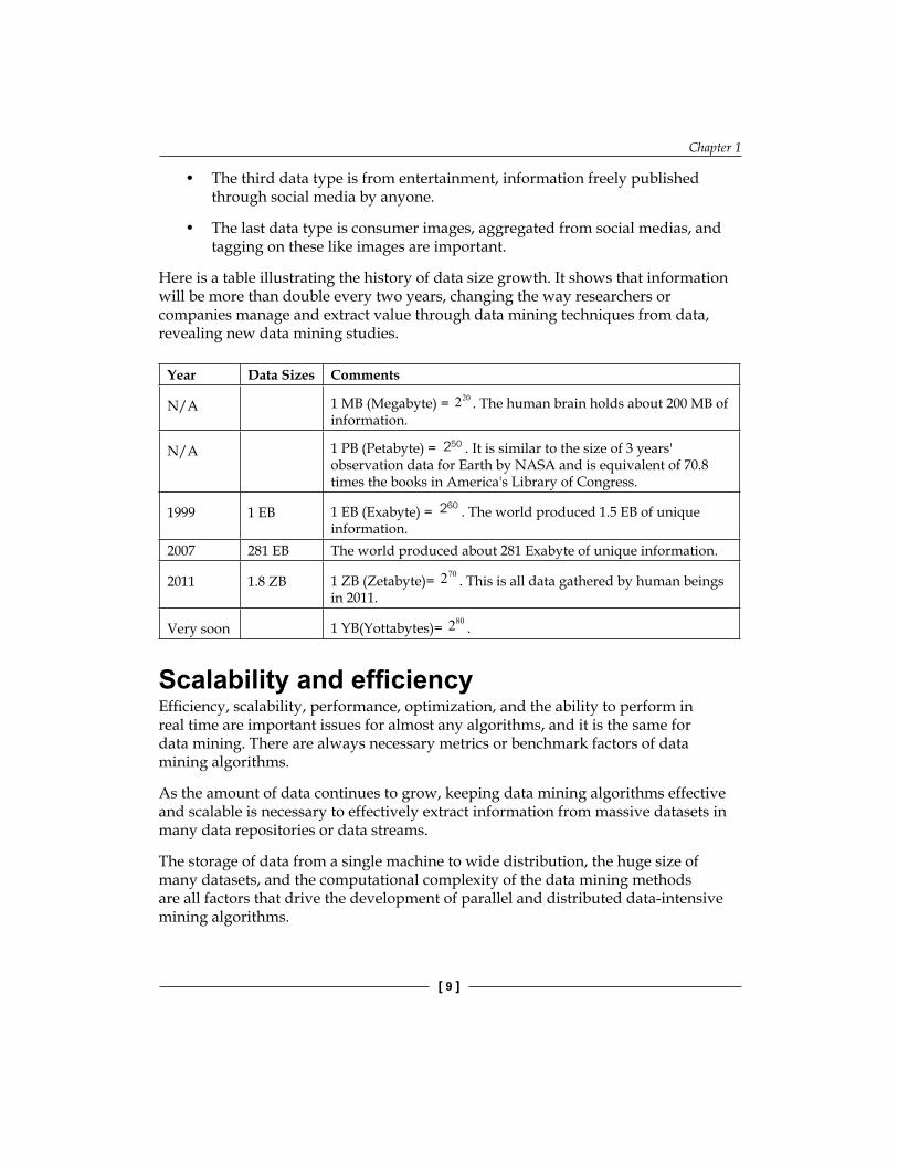
Here is a table illustrating the history of data size growth. It shows that information will be more than double every two years, changing the way researchers or companies manage and extract value through data mining techniques from data, revealing new data mining studies.

Year Data Sizes Comments

N/A 1 MB (Megabyte) = 202 . The human brain holds about 200 MB of information.

N/A 1 PB (Petabyte) = 250 . It is similar to the size of 3 years' observation data for Earth by NASA and is equivalent of 70.8 times the books in America's Library of Congress.

1999 1 EB 1 EB (Exabyte) = 260 . The world produced 1.5 EB of unique information.

2007 281 EB The world produced about 281 Exabyte of unique information.

2011 1.8 ZB 1 ZB (Zetabyte)= 702 . This is all data gathered by human beings in 2011.

Very soon 1 YB(Yottabytes)= 802 .

Scalability and effi ciencyEffi ciency, scalability, performance, optimization, and the ability to perform in real time are important issues for almost any algorithms, and it is the same for data mining. There are always necessary metrics or benchmark factors of data mining algorithms.

As the amount of data continues to grow, keeping data mining algorithms effective and scalable is necessary to effectively extract information from massive datasets in many data repositories or data streams.

The storage of data from a single machine to wide distribution, the huge size of many datasets, and the computational complexity of the data mining methods are all factors that drive the development of parallel and distributed data-intensive mining algorithms.

Warming Up

[ 10 ]

Data sourceData serves as the input for the data mining system and data repositories are important. In an enterprise environment, database and logfi les are common sources. In web data mining, web pages are the source of data. The data that continuously fetched various sensors are also a typical data source.

Here are some free online data sources particularly helpful to learn about data mining:

• Frequent Itemset Mining Dataset Repository: A repository with datasets for methods to find frequent itemsets (http://fimi.ua.ac.be/data/).

• UCI Machine Learning Repository: This is a collection of dataset, suitable for classification tasks (http://archive.ics.uci.edu/ml/).

• The Data and Story Library at statlib: DASL (pronounced "dazzle") is an online library of data files and stories that illustrate the use of basic statistics methods. We hope to provide data from a wide variety of topics so that statistics teachers can find real-world examples that will be interesting to their students. Use DASL's powerful search engine to locate the story or data file of interest. (http://lib.stat.cmu.edu/DASL/)

• WordNet: This is a lexical database for English (http://wordnet.princeton.edu)

Data miningData mining is the discovery of a model in data; it's also called exploratory data analysis, and discovers useful, valid, unexpected, and understandable knowledge from the data. Some goals are shared with other sciences, such as statistics, artifi cial intelligence, machine learning, and pattern recognition. Data mining has been frequently treated as an algorithmic problem in most cases. Clustering, classifi cation, association rule learning, anomaly detection, regression, and summarization are all part of the tasks belonging to data mining.

The data mining methods can be summarized into two main categories of data mining problems: feature extraction and summarization.

Chapter 1

[ 11 ]

Feature extractionThis is to extract the most prominent features of the data and ignore the rest. Here are some examples:

• Frequent itemsets: This model makes sense for data that consists of baskets of small sets of items.

• Similar items: Sometimes your data looks like a collection of sets and the objective is to fi nd pairs of sets that have a relatively large fraction of their elements in common. It's a fundamental problem of data mining.

SummarizationThe target is to summarize the dataset succinctly and approximately, such as clustering, which is the process of examining a collection of points (data) and grouping the points into clusters according to some measure. The goal is that points in the same cluster have a small distance from one another, while points in different clusters are at a large distance from one another.

The data mining processThere are two popular processes to defi ne the data mining process in different perspectives, and the more widely adopted one is CRISP-DM:

• Cross-Industry Standard Process for Data Mining (CRISP-DM)• Sample, Explore, Modify, Model, Assess (SEMMA), which was developed

by the SAS Institute, USA

Warming Up

[ 12 ]

CRISP-DMThere are six phases in this process that are shown in the following fi gure; it is not rigid, but often has a great deal of backtracking:

Business

Understanding

Data

Understanding

Data

Preparation

Deployment

Modeling

Evaluation

Data

Let's look at the phases in detail:

• Business understanding: This task includes determining business objectives, assessing the current situation, establishing data mining goals, and developing a plan.

• Data understanding: This task evaluates data requirements and includes initial data collection, data description, data exploration, and the verifi cation of data quality.

• Data preparation: Once available, data resources are identifi ed in the last step. Then, the data needs to be selected, cleaned, and then built into the desired form and format.

Chapter 1

[ 13 ]

• Modeling: Visualization and cluster analysis are useful for initial analysis. The initial association rules can be developed by applying tools such as generalized rule induction. This is a data mining technique to discover knowledge represented as rules to illustrate the data in the view of causal relationship between conditional factors and a given decision/outcome. The models appropriate to the data type can also be applied.

• Evaluation :The results should be evaluated in the context specifi ed by the business objectives in the fi rst step. This leads to the identifi cation of new needs and in turn reverts to the prior phases in most cases.

• Deployment: Data mining can be used to both verify previously held hypotheses or for knowledge.

SEMMAHere is an overview of the process for SEMMA:

Variable

selection,

creation

Sampling

yes/no

Data

visualization

Neural

networks

Tree-

based

models

Model

assessment

Clustering,

associations

Data

transformation

Logistic

models

Other

stat

models

SAMPLE

EXPLORE

MODIFY

MODEL

ASSESS

Let's look at these processes in detail:

• Sample: In this step, a portion of a large dataset is extracted• Explore: To gain a better understanding of the dataset, unanticipated trends

and anomalies are searched in this step• Modify: The variables are created, selected, and transformed to focus on the

model construction process

Warming Up

[ 14 ]

• Model: A variable combination of models is searched to predict a desired outcome

• Assess: The fi ndings from the data mining process are evaluated by its usefulness and reliability

Social network miningAs we mentioned before, data mining fi nds a model on data and the mining of social network fi nds the model on graph data in which the social network is represented.

Social network mining is one application of web data mining; the popular applications are social sciences and bibliometry, PageRank and HITS, shortcomings of the coarse-grained graph model, enhanced models and techniques, evaluation of topic distillation, and measuring and modeling the Web.

Social networkWhen it comes to the discussion of social networks, you will think of Facebook, Google+, LinkedIn, and so on. The essential characteristics of a social network are as follows:

• There is a collection of entities that participate in the network. Typically, these entities are people, but they could be something else entirely.

• There is at least one relationship between the entities of the network. On Facebook, this relationship is called friends. Sometimes, the relationship is all-or-nothing; two people are either friends or they are not. However, in other examples of social networks, the relationship has a degree. This degree could be discrete, for example, friends, family, acquaintances, or none as in Google+. It could be a real number; an example would be the fraction of the average day that two people spend talking to each other.

• There is an assumption of nonrandomness or locality. This condition is the hardest to formalize, but the intuition is that relationships tend to cluster. That is, if entity A is related to both B and C, then there is a higher probability than average that B and C are related.

Chapter 1

[ 15 ]

Here are some varieties of social networks:

• Telephone networks: The nodes in this network are phone numbers and represent individuals

• E-mail networks: The nodes represent e-mail addresses, which represent individuals

• Collaboration networks: The nodes here represent individuals who published research papers; the edge connecting two nodes represent two individuals who published one or more papers jointly

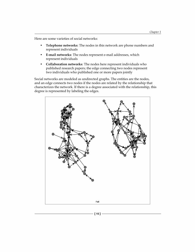
Social networks are modeled as undirected graphs. The entities are the nodes, and an edge connects two nodes if the nodes are related by the relationship that characterizes the network. If there is a degree associated with the relationship, this degree is represented by labeling the edges.

Warming Up

[ 16 ]

Downloading the example codeYou can download the example code fi les from your account at http://www.packtpub.com for all the Packt Publishing books you have purchased. If you purchased this book elsewhere, you can visit http://www.packtpub.com/support and register to have the fi les e-mailed directly to you.

Here is an example in which Coleman's High School Friendship Data from the sna R package is used for analysis. The data is from a research on friendship ties between 73 boys in a high school in one chosen academic year; reported ties for all informants are provided for two time points (fall and spring). The dataset's name is coleman, which is an array type in R language. The node denotes a specifi c student and the line represents the tie between two students.

Chapter 1

[ 17 ]

Text miningText mining is based on the data of text, concerned with exacting relevant information from large natural language text, and searching for interesting relationships, syntactical correlation, or semantic association between the extracted entities or terms. It is also defi ned as automatic or semiautomatic processing of text. The related algorithms include text clustering, text classifi cation, natural language processing, and web mining.

One of the characteristics of text mining is text mixed with numbers, or in other point of view, the hybrid data type contained in the source dataset. The text is usually a collection of unstructured documents, which will be preprocessed and transformed into a numerical and structured representation. After the transformation, most of the data mining algorithms can be applied with good effects.

The process of text mining is described as follows:

• Text mining starts from preparing the text corpus, which are reports, letters and so forth

• The second step is to build a semistructured text database that is based on the text corpus

• The third step is to build a term-document matrix in which the term frequency is included

• The fi nal result is further analysis, such as text analysis, semantic analysis, information retrieval, and information summarization

Information retrieval and text miningInformation retrieval is to help users fi nd information, most commonly associated with online documents. It focuses on the acquisition, organization, storage, retrieval, and distribution for information. The task of Information Retrieval (IR) is to retrieve relevant documents in response to a query. The fundamental technique of IR is measuring similarity. Key steps in IR are as follows:

• Specify a query. The following are some of the types of queries: ° Keyword query: This is expressed by a list of keywords to find

documents that contain at least one keyword ° Boolean query: This is constructed with Boolean operators

and keywords ° Phrase query: This is a query that consists of a sequence of words

that makes up a phrase

Warming Up

[ 18 ]

° Proximity query: This is a downgrade version of the phrase queries and can be a combination of keywords and phrases

° Full document query: This query is a full document to find other documents similar to the query document

° Natural language questions: This query helps to express users' requirements as a natural language question

• Search the document collection.• Return the subset of relevant documents.

Mining text for predictionPrediction of results from text is just as ambitious as predicting numerical data mining and has similar problems associated with numerical classifi cation. It is generally a classifi cation issue.

Prediction from text needs prior experience, from the sample, to learn how to draw a prediction on new documents. Once text is transformed into numeric data, prediction methods can be applied.

Web data miningWeb mining aims to discover useful information or knowledge from the web hyperlink structure, page, and usage data. The Web is one of the biggest data sources to serve as the input for data mining applications.

Web data mining is based on IR, machine learning (ML), statistics, pattern recognition, and data mining. Web mining is not purely a data mining problem because of the heterogeneous and semistructured or unstructured web data, although many data mining approaches can be applied to it.

Web mining tasks can be defi ned into at least three types:

• Web structure mining: This helps to fi nd useful information or valuable structural summary about sites and pages from hyperlinks

• Web content mining: This helps to mine useful information from web page contents

• Web usage mining: This helps to discover user access patterns from web logs to detect intrusion, fraud, and attempted break-in

Chapter 1

[ 19 ]

The algorithms applied to web data mining are originated from classical data mining algorithms. They share many similarities, such as the mining process; however, differences exist too. The characteristics of web data mining makes it different from data mining for the following reasons:

• The data is unstructured• The information of the Web keeps changing and the amount of data

keeps growing• Any data type is available on the Web, such as structured and

unstructured data• Heterogeneous information is on the web; redundant pages are present too• Vast amounts of information on the web is linked• The data is noisy

Web data mining differentiates from data mining by the huge dynamic volume of source dataset, a big variety of data format, and so on. The most popular data mining tasks related to the Web are as follows:

• Information extraction (IE): The task of IE consists of a couple of steps, tokenization, sentence segmentation, part-of-speech assignment, named entity identifi cation, phrasal parsing, sentential parsing, semantic interpretation, discourse interpretation, template fi lling, and merging.

• Natural language processing (NLP): This researches the linguistic characteristics of human-human and human-machine interactive, models of linguistic competence and performance, frameworks to implement process with such models, processes'/models' iterative refi nement, and evaluation techniques for the result systems. Classical NLP tasks related to web data mining are tagging, knowledge representation, ontologies, and so on.

• Question answering: The goal is to fi nd the answer from a collection of text to questions in natural language format. It can be categorized into slot fi lling, limited domain, and open domain with bigger diffi culties for the latter. One simple example is based on a predefi ned FAQ to answer queries from customers.

• Resource discovery: The popular applications are collecting important pages preferentially; similarity search using link topology, topical locality and focused crawling; and discovering communities.

Warming Up

[ 20 ]

Why R?R is a high-quality, cross-platform, fl exible, widely used open source, free language for statistics, graphics, mathematics, and data science—created by statisticians for statisticians.

R contains more than 5,000 algorithms and millions of users with domain knowledge worldwide, and it is supported by a vibrant and talented community of contributors. It allows access to both well-established and experimental statistical techniques.

R is a free, open source software environment maintained by R-projects for statistical computing and graphics, and the R source code is available under the terms of the Free Software Foundation's GNU General Public License. R compiles and runs on a wide variety for a variety of platforms, such as UNIX, LINUX, Windows, and Mac OS.

What are the disadvantages of R?There are three shortages of R:

• One is that it is memory bound, so it requires the entire dataset store in memory (RAM) to achieve high performance, which is also called in-memory analytics.

• Similar to other open source systems, anyone can create and contribute package with strict or less testing. In other words, packages contributing to R communities are bug-prone and need more testing to ensure the quality of codes.

• R seems slow than some other commercial languages.

Fortunately, there are packages available to overcome these problems. There are some solutions that can be categorized as parallelism solutions; the essence here is to spread work across multiple CPUs that overcome the R shortages that were just listed. Good examples include, but are not limited to, RHadoop. You will read more on this topic soon in the following sections. You can download the SNOW add-on package and the Parallel add-on package from Comprehensive R Archive Network (CRAN).

StatisticsStatistics studies the collection, analysis, interpretation or explanation, and presentation of data. It serves as the foundation of data mining and the relations will be illustrated in the following sections.

Chapter 1

[ 21 ]

Statistics and data miningStatisticians were the fi rst to use the term data mining. Originally, data mining was a derogatory term referring to attempts to extract information that was not supported by the data. To some extent, data mining constructs statistical models, which is an underlying distribution, used to visualize data.

Data mining has an inherent relationship with statistics; one of the mathematical foundations of data mining is statistics, and many statistics models are used in data mining.

Statistical methods can be used to summarize a collection of data and can also be used to verify data mining results.

Statistics and machine learningAlong with the development of statistics and machine learning, there is a continuum between these two subjects. Statistical tests are used to validate the machine learning models and to evaluate machine learning algorithms. Machine learning techniques are incorporated with standard statistical techniques.

Statistics and RR is a statistical programming language. It provides a huge amount of statistical functions, which are based on the knowledge of statistics. Many R add-on package contributors come from the fi eld of statistics and use R in their research.

The limitations of statistics on data miningDuring the evolution of data mining technologies, due to statistical limits on data mining, one can make errors by trying to extract what really isn't in the data.

Bonferroni's Principle is a statistical theorem otherwise known as Bonferroni correction. You can assume that big portions of the items you fi nd are bogus, that is, the items returned by the algorithms dramatically exceed what is assumed.

Warming Up

[ 22 ]

Machine learningThe data to which a ML algorithm is applied is called a training set, which consists of a set of pairs (x, y), called training examples. The pairs are explained as follows:

• x: This is a vector of values, often called the feature vector. Each value, or feature, can be categorical (values are taken from a set of discrete values, such as {S, M, L}) or numerical.

• y: This is the label, the classifi cation or regression values for x.

The objective of the ML process is to discover a function ( )y f x= that best predicts the value of y associated with each value of x. The type of y is in principle arbitrary, but there are several common and important cases.

• y: This is a real number. The ML problem is called regression.• y: This is a Boolean value true or false, more commonly written as +1 and -1,

respectively. In this class, the problem is binary classifi cation.• y: Here this is a member of some fi nite set. The member of this set can be

thought of as classes, and each member represents one class. The problem is multiclass classifi cation.

• y: This is a member of some potentially infi nite set, for example, a parse tree for x, which is interpreted as a sentence.

Until now, machine learning has not proved successful in situations where we can describe the goals of the mining more directly. Machine learning and data mining are two different topics, although some algorithms are shared between them—algorithms are shared especially when the goal is to extract information. There are situations where machine learning makes sense. The typical one is when we have idea of what we looking for in the dataset.

Approaches to machine learningThe major classes of algorithms are listed here. Each is distinguished by the function f .

• Decision tree: This form of f is a tree and each node of the tree has a function of x that determines which child or children the search must proceed for.

• Perceptron: These are threshold functions applied to the components of the vector 1 2{ , ,.. }. nx x x x= . A weight iw is associated with the ith components, for each i = 1, 2, … n, and there is a threshold

1

ni ii

w x θ=

≥∑ . The output is +1 if and the output is -1 otherwise.

Chapter 1

[ 23 ]

• Neural nets: These are acyclic networks of perceptions, with the outputs of some perceptions used as inputs to others.

• Instance-based learning: This uses the entire training set to represent the function f .

• Support-vector machines: The result of this class is a classifi er that tends to be more accurate on unseen data. The target for class separation denotes as looking for the optimal hyper-plane separating two classes by maximizing the margin between the classes' closest points.

Machine learning architectureThe data aspects of machine learning here means the way data is handled and the way it is used to build the model.

• Training and testing: Assuming all the data is suitable for training, separate out a small fraction of the available data as the test set; use the remaining data to build a suitable model or classifi er.

• Batch versus online learning: The entire training set is available at the beginning of the process for batch mode; the other one is online learning, where the training set arrives in a stream and cannot be revisited after it is processed.

• Feature selection: This helps to fi gure out what features to use as input to the learning algorithm.

• Creating a training set: This helps to create the label information that turns data into a training set by hand.

Data attributes and descriptionAn attribute is a fi eld representing a certain feature, characteristic, or dimensions of a data object.

In most situations, data can be modeled or represented with a matrix, columns for data attributes, and rows for certain data records in the dataset. For other cases, that data cannot be represented with matrices, such as text, time series, images, audio, video, and so forth. The data can be transformed into a matrix by appropriate methods, such as feature extraction.

Warming Up

[ 24 ]

The type of data attributes arises from its contexts or domains or semantics, and there are numerical, non-numerical, categorical data types or text data. Two views applied to data attributes and descriptions are widely used in data mining and R. They are as follows:

• Data in algebraic or geometric view: The entire dataset can be modeled into a matrix; linear algebraic and abstract algebra plays an important role here.

• Data in probability view: The observed data is treated as multidimensional random variables; each numeric attribute is a random variable. The dimension is the data dimension. Irrespective of whether the value is discrete or continuous, the probability theory can be applied here.

To help you learn R more naturally, we shall adopt a geometric, algebraic, and probabilistic view of the data.

Here is a matrix example. The number of columns is determined by m, which is the dimensionality of data. The number of rows is determined by n, which is the size of dataset.

( )11 1 1

1

1

m

m

n nm n

x x xA X X

x x x

⎛ ⎞ ⎛ ⎞⎜ ⎟ ⎜ ⎟= = =⎜ ⎟ ⎜ ⎟⎜ ⎟ ⎜ ⎟⎝ ⎠ ⎝ ⎠

L

M O M M L

L

Where ix denotes the i row, which is an m-tuple as follows:

( )1 1( , ,i i ix x x x= = L I

And jx denotes the j column, which is an n-tuple as follows:

( )1 1( , ,j j j njX X X X= = L

Numeric attributesNumerical data is convenient to deal with because it is quantitative and allows arbitrary calculations. The properties of numerical data are the same as integer or fl oat data.

Chapter 1

[ 25 ]

Numeric attributes taken from a fi nite or countable infi nite set of values are called discrete, for example a human being's age, which is the integer value starting from 1,150. Other attributes taken from any real values are called continuous. There are two main kinds of numeric types:

• Interval-scaled: This is the quantitative value, measured on a scale of equal unit, such as the weight of some certain fi sh in the scale of international metric, such as gram or kilogram.

• Ratio-scaled: This value can be computed by ratios between values in addition to differences between values. It is a numeric attribute with an inherent zero-point; hence, we can say a value is a multiple of another value.

Categorical attributesThe values of categorical attributes come from a set-valued domain composed of a set of symbols, such as the size of human costumes that are categorized as {S, M, L}. The categorical attributes can be divided into two groups or types:

• Nominal: The values in this set are unordered and are not quantitative; only the equality operation makes sense here.

• Ordinal: In contrast to the nominal type, the data has an ordered meaning here. The inequality operation is available here in addition to the equality operation.

Data descriptionThe basic description can be used to identify features of data, distinguish noise, or outliers. A couple of basic statistical descriptions are as follows:

• Measures of central tendency: This measures the location of middle or center of a data distribution: the mean, median, mode, midrange, and so on.

• Measure of the dispersion of the data: This is the range, quartiles, interquartile range, and so on.

Data measuringData measuring is used in clustering, outlier detection, and classifi cation. It refers to measures of proximity, similarity, and dissimilarity. The similarity value, a real value, between two tuples or data records ranges from 0 to 1, the higher the value the greater the similarity between tuples. Dissimilarity works in the opposite way; the higher the dissimilarity value, the more dissimilar are the two tuples.

Warming Up

[ 26 ]

For a dataset, data matrix stores the n data tuples in n x m matrix (n tuples and m attributes):

11 1

1

m

n nm

x x

x x

⎛ ⎞⎜ ⎟⎜ ⎟⎜ ⎟⎝ ⎠

L

M O M

L

The dissimilarity matrix stores a collection of proximities available for all n tuples in the dataset, often in a n x n matrix. In the following matrix, ( ),d i j means the dissimilarity between two tuples; value 0 for highly similar or near between each other, 1 for completely same, the higher the value, the more dissimilar it is.

( )( ) ( )

( ) ( )

2,1 03,1 3,2 0

,1 ,2 0

0d

d d

d n d n

⎛ ⎞⎜ ⎟⎜ ⎟⎜ ⎟⎜ ⎟⎜ ⎟⎜ ⎟…⎝ ⎠

MMM

Most of the time, the dissimilarity and similarity are related concepts. The similarity measure can often be defi ned using a function; the expression constructed with measures of dissimilarity, and vice versa.

Here is a table with a list of some of the most used measures for different attribute value types:

Attribute value types DissimilarityNominal attributes The dissimilarity between two tuples can be computed by the

following equation: d (i, j) = (p-m)/pWhere, p is the dimension of data and m is the number of matches that is in same state.

Ordinal attributes The treatment of ordinal attributes is similar to that of numeric attributes, but it needs a transformation first before applying the methods.

Interval-scaled Euclidean, Manhattan, and Minkowski distances are used to calculate the dissimilarity of data tuples.

Chapter 1

[ 27 ]

Data cleaningData cleaning is one part of data quality. The aim of Data Quality (DQ) is to have the following:

• Accuracy (data is recorded correctly)• Completeness (all relevant data is recorded)• Uniqueness (no duplicated data record)• Timeliness (the data is not old)• Consistency (the data is coherent)

Data cleaning attempts to fi ll in missing values, smooth out noise while identifying outliers, and correct inconsistencies in the data. Data cleaning is usually an iterative two-step process consisting of discrepancy detection and data transformation.

The process of data mining contains two steps in most situations. They are as follows:

• The fi rst step is to perform audition on the source dataset to fi nd the discrepancy.

• The second step is to choose the transformation to fi x (based on the accuracy of the attribute to be modifi ed and the closeness of the new value to the original value). This is followed by applying the transformation to correct the discrepancy.

Missing valuesDuring the process to seize data from all sorts of data sources, there are many cases when some fi elds are left blank or contain a null value. Good data entry procedures should avoid or minimize the number of missing values or errors. The missing values and defaults are indistinguishable.

If some fi elds are missing a value, there are a couple of solutions—each with different considerations and shortages and each is applicable within a certain context.

• Ignore the tuple: By ignoring the tuple, you cannot make use of the remaining values except the missing one. This method is applicable when the tuple contains several attributes with missing values or the percentage of missing value per attribute doesn't vary considerably.

• Filling the missing value manually: This is not applicable for large datasets.• Use a global constant to fi ll the value: Applying the value to fi ll the missing

value will misguide the mining process, and is not foolproof.

Warming Up

[ 28 ]

• Use a measure for a central tendency for the attribute to fi ll the missing value: The measures of central tendency can be used for symmetric data distribution.

• Use the attribute mean or median: Use the attribute mean or median for all samples belonging to the same class as the given tuple.

• Use the most probable value to fi ll the missing value: The missing data can be fi lled with data determined with regression, inference-based tool, such as Bayesian formalism or decision tree induction.

The most popular method is the last one; it is based on the present values and values from other attributes.

Junk, noisy data, or outlierAs in a physics or statistics test, noise is a random error that occurs during the test process to seize the measured data. No matter what means you apply to the data gathering process, noise inevitably exists.

Approaches for data smoothing are listed here. Along with the progress of data mining study, new methods keep occurring. Let's have a look at them:

• Binning: This is a local scope smoothing method in which the neighborhood values are used to compute the fi nal value for the certain bin. The sorted data is distributed into a number of bins and each value in that bin will be replaced by a value depending on some certain computation of the neighboring values. The computation can be bin median, bin boundary, which is the boundary data of that bin.

• Regression: The target of regression is to fi nd the best curve or something similar to one in a multidimensional space; as a result, the other values will be used to predict the value of the target attribute or variable. In other aspects, it is a popular means for smoothing.

• Classifi cation or outlier: The classifi er is another inherent way to fi nd the noise or outlier. During the process of classifying, most of the source data is grouped into couples of groups, except the outliers.

Chapter 1

[ 29 ]

Data integrationData integration combines data from multiple sources to form a coherent data store. The common issues here are as follows:

• Heterogeneous data: This has no common key• Different defi nition: This is intrinsic, that is, same data with different

defi nition, such as a different database schema• Time synchronization: This checks if the data is gathered under same

time periods• Legacy data: This refers to data left from the old system• Sociological factors: This is the limit of data gathering

There are several approaches that deal with the above issues:

• Entity identifi cation problem: Schema integration and object matching are tricky. This referred to as the entity identifi cation problem.

• Redundancy and correlation analysis: Some redundancies can be detected by correlation analysis. Given two attributes, such an analysis can measure how strongly one attribute implies the other, based on the available data.

• Tuple Duplication: Duplication should be detected at the tuple level to detect redundancies between attributes

• Data value confl ict detection and resolution: Attributes may differ on the abstraction level, where an attribute in one system is recorded at a different abstraction level

Data dimension reductionReduction of dimensionality is often necessary in the analysis of complex multivariate datasets, which is always in high-dimensional format. So, for example, problems modeled by the number of variables present, the data mining tasks on the multidimensional analysis of qualitative data. There are also many methods for data dimension reduction for qualitative data.

The goal of dimensionality reduction is to replace large matrix by two or more other matrices whose sizes are much smaller than the original, but from which the original can be approximately reconstructed, usually by taking their product with loss of minor information.

Warming Up

[ 30 ]

Eigenvalues and EigenvectorsAn eigenvector for a matrix is defi ned as when the matrix (A in the following equation) is multiplied by the eigenvector (v in the following equation). The result is a constant multiple of the eigenvector. That constant is the eigenvalue associated with this eigenvector. A matrix may have several eigenvectors.

Av vλ=

An eigenpair is the eigenvector and its eigenvalue, that is, ( ,ν λ ) in the preceding equation.

Principal-Component AnalysisThe Principal-Component Analysis (PCA) technique for dimensionality reduction views data that consists of a collection of points in a multidimensional space as a matrix, in which rows correspond to the points and columns to the dimensions.

The product of this matrix and its transpose has eigenpairs, and the principal eigenvector can be viewed as the direction in the space along which the points best line up. The second eigenvector represents the direction in which deviations from the principal eigenvector are the greatest.

Dimensionality reduction by PCA is to approximate the data by minimizing the root-mean-square error for the given number of columns in the representing matrix, by representing the matrix of points by a small number of its eigenvectors.

Singular-value decompositionThe singular-value decomposition (SVD) of a matrix consists of following three matrices:

• U• ∑• V

U and V are column-orthonormal; as vectors, the columns are orthogonal and their length is 1. ∑ is a diagonal matrix and the values along its diagonal are called singular values. The original matrix equals to the product of U, ∑, and the transpose of V.

SVD is useful when there are a small number of concepts that connect the rows and columns of the original matrix.

Chapter 1

[ 31 ]

Dimensionality reduction by SVD for matrix U and V are typically as large as the original. To use fewer columns for U and V, delete the columns corresponding to the smallest singular values from U, V, and ∑. This minimizes the error in reconstruction of the original matrix from the modifi ed U, ∑, and V.

CUR decompositionThe CUR decomposition seeks to decompose a sparse matrix into sparse, smaller matrices whose product approximates the original matrix.

The CUR chooses from a given sparse matrix a set of columns C and a set of rows R, which play the role of U and TV in SVD. The choice of rows and columns is made randomly with a distribution that depends on the square root of the sum of the squares of the elements. Between C and R is a square matrix called U, which is constructed by a pseudo-inverse of the intersection of the chosen rows and columns.

By CUR solution, the three component matrices C, U, and R will be retrieved. The product of those three will approximate the original matrix M. For R community, rCUR is an R package for the CUR matrix decomposition.

Data transformation and discretizationAs we know from the previous section, there are always some data formats that are best suited for specifi c data mining algorithms. Data transformation is an approach to transform the original data to preferable data format for the input of certain data mining algorithms before the processing.

Data transformationData transformation routines convert the data into appropriate forms for mining. They're shown as follows:

• Smoothing: This uses binning, regression, and clustering to remove noise from the data

• Attribute construction: In this routine, new attributes are constructed and added from the given set of attributes

• Aggregation: In this summary or aggregation, operations are performed on the data

Warming Up

[ 32 ]

• Normalization: Here, the attribute data is scaled so as to fall within a smaller range

• Discretization: In this routine, the raw values of a numeric attribute are replaced by interval label or conceptual label

• Concept hierarchy generation for nominal data: Here, attributes can be generalized to higher level concepts

Normalization data transformation methods To avoid dependency on the choice of measurement units on data attributes, the data should be normalized. This means transforming or mapping the data to a smaller or common range. All attributes gain an equal weight after this process. There are many normalization methods. Let's have a look at some of them:

• Min-max normalization: This preserves the relationships among the original data values and performs a linear transformation on the original data. The applicable ones of the actual maximum and minimum values of an attribute will be normalized.

• z-score normalization: Here the values for an attribute are normalized based on the mean and standard deviation of that attribute. It is useful when the actual minimum and maximum of an attribute to be normalized are unknown.

• Normalization by decimal scaling: This normalizes by moving the decimal point of values of attribute.

Data discretizationData discretization transforms numeric data by mapping values to interval or concept labels. Discretization techniques include the following:

• Data discretization by binning: This is a top-down unsupervised splitting technique based on a specifi ed number of bins.

• Data discretization by histogram analysis: In this technique, a histogram partitions the values of an attribute into disjoint ranges called buckets or bins. It is also an unsupervised method.

• Data discretization by cluster analysis: In this technique, a clustering algorithm can be applied to discretize a numerical attribute by partitioning the values of that attribute into clusters or groups.

Chapter 1

[ 33 ]

• Data discretization by decision tree analysis: Here, a decision tree employs a top-down splitting approach; it is a supervised method. To discretize a numeric attribute, the method selects the value of the attribute that has minimum entropy as a split-point, and recursively partitions the resulting intervals to arrive at a hierarchical discretization.

• Data discretization by correlation analysis: This employs a bottom-up approach by fi nding the best neighboring intervals and then merging them to form larger intervals, recursively. It is supervised method.

Visualization of resultsVisualization is the graphic presentation of data-portrayals meant to reveal complex information at a glance, referring to all types of structured representation of information. This includes graphs, charts, diagrams, maps, storyboards, and other structured illustrations.

Good visualization of results gives you the chance to look at data through the eyes of experts. It is beautiful not only for their aesthetic design, but also for the elegant layers of detail that effi ciently generate insight and new understanding.

The result of every data mining algorithm can be visualized and clarifi ed by the use of the algorithms. Visualization plays an important role in the data mining process.

There are four major features that create the best visualizations:

• Novel: It must not only merely being a conduit for information, but offer some novelty in the form of new style of information.

• Informative: The attention to these factors and the data itself will make a data visualization effective, successful, and beautiful.

• Effi cient: A nice visualization has an explicit goal, a clearly defi ned message, or a special perspective on the information that it is made to convey. It must be as simple as possible and straightforward, but shouldn't lose out on necessary, relevant complexity. The irrelevant data serves as noises here. It should refl ect the qualities of the data that they represent, reveal properties and relationships inherent and implicit in the data source to bring new knowledge, insight, and enjoyment to fi nal user.

• Aesthetic: The graphic must serve the primary goal of presenting information, not only axes and layout, shapes, lines, and typography, but also the appropriate usage of these ingredients.

Warming Up

[ 34 ]

Visualization with RR provides the production of publication-quality diagrams and plots. There are graphic facilities distributed with R, and also some facilities that are not part of the standard R installation. You can use R graphics from command line.

The most important feature of the R graphics setup is the existence of two distinct graphics systems within R:

• The traditional graphics system• Grid graphics system

The most appropriate facilities will be evaluated and applied to the visualization of every result of all algorithms listed in the book.

Functions in the graphics systems and add-on packages can be divided into several types:

• High-level functions that produce complete plots• Low-level functions to add further output to an existing plot• The ones to work interactively with graphical output

R graphics output can be produced in a wide range of graphical formats, such as PNG, JPEG, BMP, TIFF, SVG, PDF, and PS.

To enhance your knowledge about this chapter, here are some practice questions for you to have check about the concepts.

Time for actionLet's now test what we've learned so far:

• What is the difference between data mining and machine learning?• What is data preprocessing and data quality?• Download R and install R on your machine.• Compare and contrast data mining and machine learning.

Chapter 1

[ 35 ]

SummaryIn this chapter, we looked at the following topics:

• An introduction to data mining and available data sources• A quick overview of R and the necessity to use R• A description of statistics and machine learning, and their relations to

data mining• The two standard industrial data mining process• Data attributes types and the data measurement approaches• The three important steps in data preprocessing• An introduction to the scalability and effi ciency of data mining algorithms,

and data visualization methods and necessities• A discussion on social network mining, text mining, and web data mining• A short introduction about RHadoop and Map Reduce

In the following chapters, the reader will learn how to implement various data mining algorithms and manipulate data with R.

Where to buy this book You can buy Learning Data Mining with R from the Packt Publishing website. Alternatively, you can buy the book from Amazon, BN.com, Computer Manuals and most internet book retailers.

Click here for ordering and shipping details.

www.PacktPub.com

Stay Connected:

Get more information Learning Data Mining with Rt