868 IEEE TRANSACTIONS ON SIGNAL PROCESSING, VOL. 62, NO. …

868 IEEE TRANSACTIONS ON SIGNAL PROCESSING, VOL. 62, NO. 4, FEBRUARY 15, 2014

Convergence Rates of Distributed Nesterov-LikeGradient Methods on Random Networks

Dušan Jakovetić, Member, IEEE, João Manuel Freitas Xavier, Member, IEEE, and José M. F. Moura, Fellow, IEEE

Abstract—We consider distributed optimization in random net-works where nodes cooperatively minimize the sumof their individual convex costs. Existing literature proposesdistributed gradient-like methods that are computationally cheapand resilient to link failures, but have slow convergence rates. Inthis paper, we propose accelerated distributed gradient methodsthat 1) are resilient to link failures; 2) computationally cheap;and 3) improve convergence rates over other gradient methods.We model the network by a sequence of independent, identicallydistributed random matrices drawn from the set ofsymmetric, stochastic matrices with positive diagonals. The net-work is connected on average and the cost functions are convex,differentiable, with Lipschitz continuous and bounded gradients.We design two distributed Nesterov-like gradient methods thatmodify the D–NG and D–NC methods that we proposed forstatic networks. We prove their convergence rates in terms ofthe expected optimality gap at the cost function. Let andbe the number of per-node gradient evaluations and per-nodecommunications, respectively. Then the modified D–NG achievesrates and , and the modified D–NC rates

and , where is arbitrarily small. Forcomparison, the standard distributed gradient method cannotdo better than and , on the same class ofcost functions (even for static networks). Simulation examplesillustrate our analytical findings.

Index Terms—Consensus, convergence rate, distributed opti-mization, Nesterov gradient, random networks.

I. INTRODUCTIONA. Motivation

W ITH many distributed signal processing applications, acommon research challenge is to develop distributed al-

gorithms whereby all nodes in a generic, connected network re-

Manuscript received May 11, 2013; revised August 14, 2013; accepted Oc-tober 03, 2013. Date of publication November 14, 2013; date of current versionJanuary 20, 2014. The associate editor coordinating the review of this manu-script and approving it for publication was Prof. Shuguang (Robert) Cui. Thework of D. Jakovetić and J. M. F. Xavier was supported by Carnegie Mellon/Portugal Program under a grant from the Fundação de Ciência e Tecnologia(FCT) from Portugal; this work was supported by FCT grants CMU-PT/SIA/0026/2009 and SFRH/BD/33518/2008 (through the Carnegie Mellon\PortugalProgram managed by ICTI); by ISR/IST pluriannual funding (POSC program,FEDER); the work of D. Jakovetić and J. M. F. Moura was supported by anAFOSR grant FA95501010291 and by an NSF grant CCF1011903, while D.Jakovetić was a doctoral and postdoctoral student within the Carnegie Mellon/Portugal Program.D. Jakovetić is with the University of Novi Sad, BioSense Center, 21000Novi

Sad, Serbia (e-mail: [email protected]).J. M. F. Xavier is with the SIPG—Signal and Image Processing Group, Insti-

tuto de Sistemas e Robótica (ISR), Instituto Superior Técnico (IST), Universityof Lisboa, 1049-001 Lisbon, Portugal (e-mail: [email protected]).J. M. F. Moura is with the Department of Electrical and Computer En-

gineering, Carnegie Mellon University, Pittsburgh, PA 15213 USA (e-mail:[email protected]).Color versions of one or more of the figures in this paper are available online

at http://ieeexplore.ieee.org.

cover a global vector parameter of common interest, whileeach node possesses only a partial, local knowledge on the un-known vector and interacts only locally, with immediateneighbors in the network. For example, such situation ariseswith (distance-measurement based) acoustic source localizationin wireless sensor networks (WSNs). Node measures the re-ceived signal energy that contains information only about itsdistance to the acoustic source, and hence node in isolationcannot recover the unknown source location; but, it can recoverthe source location by collaborating with other nodes in the net-work (see Example 3 below for details). In many applications,like with WSNs, the inter-node communications are prone torandom communication failures (e.g., random packet dropoutsin WSNs); an important challenge in developing distributed al-gorithms to recover is to make them provably resilient torandom communication failures.Similarly to, e.g., [1]–[3], we address the above problem in

the framework of distributed (smooth) optimization. Each nodein a generic, connected network has a differentiable, convexcost function known only by node , parameterizedby node ’s local data , with the global optimizationvariable common to all nodes. Each node in the network wantsto find a parameter that minimizes the sum of thenodes’ local costs :

(1)

where we assume that each has Lipschitz continuous andbounded gradients. In this paper, our goals are: 1) to developdistributed, iterative, gradient-based methods that solve (1),whereby nodes over iterations exchange messages only withtheir immediate neighbors; and 2) to provide convergence rateguarantees of the methods (on the assumed functions class) inthe presence of random communication failures.We now motivate setup (1) with three application examples

from the literature, namely 1) distributed learning of a linearclassifier, 2) distributed robust estimation, and 3) distributedsource localization. Each of the three example problemsobeys the Assumptions that we make on the ’s (see aheadAssumptions 3, 4, and 5 for details.) Besides those, existingliterature provides many other application examples, includingdistributed estimation, e.g., [4]–[6], distributed detection, e.g.,[7], [8], target localization and intruder detection in biologicalnetworks, e.g., [9], and spectrum sensing for cognitive radionetworks, e.g., [10].1) Example 1: Distributed Learning of a Linear Classifier:

Consider a distributed learning scenario where training data isdistributed across nodes in the network; each node has datasamples, , where is a feature vector and

1053-587X © 2013 IEEE. Personal use is permitted, but republication/redistribution requires IEEE permission.See http://www.ieee.org/publications_standards/publications/rights/index.html for more information.

JAKOVETIĆ et al.: DISTRIBUTED NESTEROV-LIKE GRADIENT METHODS 869

is the class label of the vector , e.g., [11]. Forthe purpose of future feature vector classifications, each nodewants to learn the linear classifier , i.e.,to determine a vector and a scalar , based onall nodes’ data samples, that yields the best classification in acertain sense. Specifically, we seek and thatsolve:

(2)

where is the logistic loss. Problem(2) fits (1), with , and

.2) Example 2: Distributed Robust Estimation in Sensor Net-

works: Consider a sensor network deployed, e.g., to measure apollution level in a certain area [12]. Each sensor makesscalar measurements (of the level of pollution), . As-sume a signal+noise measurement model, where ,with the “signal” (real pollution level), and a zero-meannoise, independent across all indices . Further, suppose thatthere are two groups of sensors, and . Sensors op-erate correctly, and their measurements have a small variance

, , ; sensorsare damaged, and their measurements have a large variance

, , . To combat the outliermeasurements from damaged sensors in , [12] estimates theparameter through the Huber loss, i.e., it obtains an estimateas a solution to the following problem:

(3)

where is the Huber loss: , if, and , otherwise.

3) Example 3: Acoustic Source Localization in SensorNetworks: Suppose that an acoustic source is positioned at anunknown location in the field [12], [13]. Each node(sensor) measures the received signal energy from the source:

Here is node ’s location (known to node ), andare constants known to all nodes, and is zero-mean

additive noise. The goal is for each node to estimate the source’sposition . Reference [13] proposes to obtain an estimate ofby solving:

(4)

where is the disk

and is the distance from to the set. It can be shown that ,

which is convex but nonsmooth. To adapt the latter functionto our setting, we take standard smooth approximations of theinvolved nonsmooth functions. Namely, we approximate

with and

with , whereis a large scalar and is a small scalar. The re-

sulting optimization problem takes the form of (1) with.

B. Contributions

We now state our main contributions by placing them in thecontext of existing work. For problem (1), [3], see also [14],[15], presents two distributed Nesterov-like gradient algorithmsfor static (non-random) networks, referred to as D–NG (Dis-tributed Nesterov Gradient algorithm) and D–NC (DistributedNesterov gradient with Consensus iterations).In this paper, we propose the mD–NG and mD–NC algo-

rithms, which modify the D–NG and D–NC algorithms, and,beyond proving their convergence, we solve the much harderproblem of establishing their convergence rate guaranteeson random networks. We model the network by a sequenceof random independent, identically distributed (i.i.d.) weightmatrices drawn from a set of symmetric, stochastic ma-trices with positive diagonals, and we assume that the networkis connected on average (the graph supporting isconnected). We establish the convergence rates of the expectedoptimality gap in the cost function (at any node ) of mD-NGand mD-NC, in terms of the number of per node gradientevaluations and the number of per-node communications, when the functions are convex and differentiable, with

Lipschitz continuous and bounded gradients. We show thatthe modified methods achieve in expectation the same ratesthat the methods in [3] achieve on static networks, namely:mD–NG converges at rates and ,while mD–NC has rates and , whereis an arbitrarily small positive number. We explicitly give theconvergence rate constants in terms of the number of nodesand the network statistics, more precisely, in terms of the

quantity (See ahead paragraphwith heading Notation.)We contrast D–NG and D–NC in [3] with their modified

variants, mD–NG and mD–NC, respectively. Simulations inSection VI show that D–NG may diverge when links fail, whilemD–NG converges, possibly at a slightly lower rate on staticnetworks and requires an additional ( -dimensional) vectorcommunication per iteration . Hence, mD–NG compromisesslightly speed of convergence for robustness to link failures.Algorithm mD–NC has one inner consensus with -dimen-

sional variables per outer iteration , while D–NC has two con-sensus algorithms with -dimensional variables. Both D–NCvariants converge in our simulations when links fail, showingsimilar performance.The analysis here differs from [3], since the dynamics of dis-

agreements are different from the dynamics in [3]. This requiresnovel bounds on certain products of time-varying matrices. Bydisagreement, we mean how different the solution estimates ofdistinct nodes are, say and for nodes and .


C. Brief Comment on the Literature

There is increased interest in distributed optimization andlearning. Broadly, the literature considers two types of methods,namely, batch processing, e.g., [1], [10], [16]–[19], and onlineadaptive processing, e.g., [4], [9], [20], [21]. With batch pro-cessing, data is acquired beforehand, and hence the ’s areknown before the algorithm runs. In contrast, with adaptive on-line processing, nodes acquire new data at each iteration of thedistributed algorithm. In general, adaptive and batch processingshow inherent tradeoffs.We comment on certain advantages anddisadvantages of the two methods. When the unknown param-eter is time-varying, and the time constant of thedynamics of is comparable with the time needed to per-form one distributed algorithm’s iteration, adaptive processingis the right choice. When the dynamics of are slow com-pared to the time needed to iterate the distributed algorithm untilconvergence, or when does not vary with time (the casewe consider here), both batch and adaptive processing can beapplied. To our best knowledge, existing literature does not ad-dress comparisons of distributed adaptive and distributed batchoptimization algorithms. A systematic comparison among thetwo types of distributed methods is a nontrivial task and is out-side of our paper’s scope. In the centralized setting, [22] ad-dresses a similar problem in machine learning, by comparingthe standard gradient method (batch processing) and the sto-chastic gradient method (adaptive/online processing). Their re-sults roughly show that, when the number of data samples issmall enough and the allowed computational cost to performoptimization is large enough, it is advantageous to use batchprocessing (standard gradient method); on the other hand, if thenumber of data samples is large enough and the allowed compu-tational cost is small enough, it is advantageous to use adaptiveprocessing (online gradient method). We consider in this paperbatch processing.Distributed gradient methods are, e.g., in [1], [2], [12],

[16]–[18], [23]–[27]. References [1], [16], [24] proved conver-gence of their algorithms under deterministically time varyingor random networks. Typically, ’s are convex, non-differ-entiable, and with bounded gradients over the constraint set.

Reference [2] establishes convergence rate(with high probability) of a version of the distributed dualaveraging method. We assume a more restricted class of costfunctions– ’s that are convex and have Lipschitz continuousand bounded gradients, but, in contradistinction, we establishstrictly faster convergence rates–at least that arenot achievable by standard distributed gradient methods [1]on the same class . Indeed, [3] shows that the method in[1] cannot achieve a worst-case rate better thanon the same class , even for static networks. Reference [28]proposes an accelerated distributed proximal gradient method,which resembles our D–NC method for deterministically timevarying networks; in contrast, we deal here with randomlyvarying networks. For a detailed comparison of D–NC with[28], we refer to [3].In addition to distributed gradient-like methods, a different

type of methods – distributed (augmented) Lagrangian and dis-tributed alternating direction of multipliers methods (ADMM)have been studied, e.g., in [10], [29]–[35]. They have in generalmore complex iterations than gradient methods, but may have a

lower total communication cost, e.g., [30]. [34] shows conver-gence of an asynchronous ADMM algorithm while [35] showsan rate (in expectation) of an asynchronous ADMMmethod studied therein.In summary, our paper differs from the existing literature by

simultaneously considering the following three problem dimen-sions. Namely, we consider (1) distributed, (2) Nesterov-like(accelerated) gradient methods that operate on (3) random net-works. To our best knowledge, neither of the exiting works con-siders these three dimensions simultaneously.

D. Paper Organization

The next paragraph sets notation. Section II introducesthe network and optimization models, reviews D–NG andD–NC in [3], and gives certain preliminary results. Section IIIpresents mD–NG, states its convergence rate, and proves therate. Section IV presents mD–NC and its convergence ratewith proofs. Section V discusses extensions to our results.Section VI illustrates mD–NG and mD–NC on a Huber lossexample. We conclude in Section VII. The remaining proofsare in the Appendix.

Notation

Denote by: the -dimensional real space: orthe entry of ; the transpose of ; the se-lection of the -th, -th, , -th entries of vector ; ,0, , and , respectively, the identity matrix, the zero matrix,the column vector with unit entries, and the -th column of ;

denotes the ideal consensus matrix;the Kronecker product of matrices; the vector (matrix)-norm of its argument; the Euclidean (spectral)norm of its vector (matrix) argument ( also denotes the mod-ulus of a scalar); the -th smallest in modulus eigenvalue;

a positive definite Hermitian matrix ; the smallestinteger greater than or equal to a real scalar ; the gra-dient at of a differentiable function , ;

and the probability and expectation, respectively. Fortwo positive sequences and , we have: if

; if ;and if , and .

II. MODEL AND PRELIMINARIES

Section II-A introduces the network and optimizationmodels,Section II-B reviews the D–NG and D–NC distributed methodsproposed in [3], and Section II-C gives preliminary results ofcertain products of time varying matrices.

A. Problem Model

1) Random Network Model: The network is random, due tolink failures or communication protocol used (e.g., gossip, [36],[37].) It is defined by a sequence of randomweight matrices.Assumption 1 (Random Network): We have:(a) The sequence is i.i.d.(b) Almost surely (a.s.), are symmetric, stochastic,

with strictly positive diagonal entries.


(c) There exists such that, for all , a.s..

By Assumptions 1 (b) and (c), a.s., ; also,, , may be zero, but if (nodes and

communicate) it is non-negligible (at least ). Assumption1 (c) is mild and standard in the analysis of consensus anddistributed gradient methods, e.g., [1], [23]. It says that a nodealways gives a non-negligible weight to itself.Let , the supergraph , the set

of nodes, and – collectsall realizable links, all pairs for which withpositive probability.2) Link Failure Model is covered by Assumption 1. This

model is suitable, e.g., for a practical WSN, where randompacket dropouts are adequately modeled by random link fail-ures. Here, each link at time is Bernoulli: whenit is one, is online (communication), and when it is zero,the link fails (no communication). The Bernoulli links areindependent over time, but may be correlated in space. Possibleweights are: 1) , : , when

is online, and , else; 2) , :; and 3) . While the

weights , here are binary random variables(taking values either or 0), the diagonal weightshave a more complex probability distribution.As noted, our network model covers intermittent link failures

but does not cover node failures, which may occur due to, e.g.,energy depletion of a node. Modeling node failures is an inter-esting topic for future work.We further make the following Assumption.Assumption 2 (Network Connectedness): is connected.Denote by , by

(5)

and by . One can show that

is the square root of the secondlargest eigenvalue of and that, under Assumptions1 and 2, . Lemma 1 (proof in Appendix A) shows thatcharacterizes the geometric decay of the first and second

moments of .Lemma 1: Let Assumptions 1 and 2 hold. Then:

(6)

(7)

(8)

for all for allThe bounds in (6)–(8) may be loose, but are enough to prove

the results below and simplify the presentation.3) Optimization Model: We now introduce the optimization

model. The nodes solve the unconstrained problem (1). Thefunction is known only to node . We imposethe following three Assumptions.Assumption 3 (Solvability): There exists a solution

such that .

Assumption 4 (Lipschitz Continuous Gradient): For all ,is convex, differentiable, and has Lipschitz continuous gradientwith constant :

Assumption 5 (Bounded Gradients): There exists a constantsuch that, , ,

Assumptions 3 and 4 are standard in gradient methods; in par-ticular, Assumption 4 is precisely the Assumption required bythe centralized Nesterov gradient method [38]. Assumption 5is not required in centralized Nesterov. Reference [3] demon-strates that (even on) static networks and a constant ,the convergence rates of D–NG or of the standard distributedgradient method in [1] become arbitrarily slow if Assumption 5is relaxed. See examples 1–3 in the introduction for the ’s thatobey Assumptions 3–5.

Algorithms D–NG and D–NC for Static Networks

We briefly review the D–NG and D–NC methods proposedin [3] for static networks. For this purpose, current subsectionassumes a static, deterministic, connected network, with anassociated symmetric, stochastic, deterministic weight matrix

, with . With D–NG, the matrixis positive definite, while with D–NC this requirement is

not needed.Algorithm D–NG: Node maintains its solution estimateand an auxiliary variable , It uses arbi-

trary initialization and, for ,performs the updates

(9)

(10)

In (9)–(10), is the neigh-borhood of node (including node ). For thestep-size is:

(11)

and is the sequence from the centralized Nesterov gradientmethod, [38]:

(12)

The D–NG algorithm works as follows. At iteration , nodereceives the variables from its neighbors ,and updates and via (9) and (10).Algorithm D–NC operates in two time scales. In the outer

(slow time scale) iterations , each node updates its solu-tion estimate , and updates an auxiliary variable (aswith the D–NG). In the inner iterations , nodes perform tworounds of consensus with the number of inner iterationsand , given by:

The D–NC algorithm is presented in Algorithm 1.


Algorithm 1: Algorithm D–NC

1: Initialization: Node sets: .2: Node calculates:3: (First consensus) Nodes run average consensus initializedby :

and set .4: Node calculates

.5: (Second consensus) Nodes run average consensusinitialized by :

and set .6: Set and go to step 2.

B. Scalar Sums and Products of Time-Varying Matrices

In the convergence rate analysis of mD–NG and mD–NC, wemake use of certain scalar sum bounds and bounds on the prod-ucts of 2 2 time varying matrices. We state these preliminaryresults here and prove them in Appendix B.Lemma 2 (Scalar Sums): Let . Then, for all

(13)

(14)

For , let be:

(15)

with in (12). Further, let and:

(16)

We have the following important result, proved in Appendix B.Lemma 3: Consider in (16). Then, for all

, for all

(17)

Algorithm mD–NG

We now present our mD–NG algorithm for random networks.Section III-A describes the algorithm, Section III-B sates ourresults on its convergence rate, and Section III-C proves theseresults.

C. The Algorithm

We modify D–NG in (9)–(10) to handle random networks.Node maintains its solution estimate and auxiliary vari-able , It uses arbitrary initialization

and, for , performs the updates

(18)

(19)

In (18)–(19), is the(random) neighborhood of node (including node ) at time .For the step-size is in (11), and the sequenceis in (12). We assume nodes know (Section V relaxes this.)The mD–NG algorithm (18)–(19) differs from D–NG in

(9)–(10) in step (19). With D–NG, nodes communicate onlythe ’s; with mD–NG, they also communicate the

’s (see the sum term in (19)). This modificationallows for the robustness to link failures. (See Theorems 4 and5 and the simulations in Section VI.) Further, mD–NG does notrequire the weight matrix to be positive definite, while D–NGdoes.1) Vector Form: Let ,

, and ,. Then, for

, with , the Kro-necker product of with the identity , mD–NG invector form is:

(20)

(21)

2) Initialization: For notation simplicity, without loss ofgenerality (wlog), we assume, with all proposed methods,that nodes initialize their estimates to the same values, i.e.,

, for all ; for example,.

3) Communication and Computational Costs, Per Node andIteration : We show the communication and computationalcosts of mD–NG per iteration and compare it with the costsof the standard distributed gradient method in [1]. Consider,for simplicity, a regular, static network, with degree (numberof neighbors of each node) . Further, suppose that the com-putational cost of computing the gradient of each is sim-ilar, . mD–NG requires, per , mul-tiplications, additions, and one gradient evaluation( ), while [1] requires multiplications,

additions, and one gradient evaluation. The cost of thegradient evaluation depends on the ’s and is usually dominantover other terms. Regarding communications per , mD–NGrequires communicated scalars per node, while [1] requirescommunicated scalars per node. Hence, compared with [1],

mD–NG has about twice larger communication cost and (lessthan) twice larger computational cost per . As we show furtherahead in Theorem 5, mD–NG has rate , while [1] is


(in a worst-case sense) no faster than , [3]. Given theserates and the fact that one iteration of mD–NG costs (roughly)as two iterations of [1], it is clear that mD–NG has a faster ratethan [1] in terms of the overall cost.

D. Convergence Rate of mD–NG

We state our convergence rate result for mD–NG. Proofsare in Section III-C. We estimate the expected optimality gapin the cost at each node normalized by , e.g., [2], [27]:

, where is node ’s solution at a certainstage of the algorithm. We study how node ’s optimality gapdecreases with: 1) the number of iterations, or of per-nodegradient evaluations; and 2) the total number of -di-mensional vector communications per node. With mD–NG,

–at each , there is one and only one per-node -dimen-sional communication and one per-node gradient evaluation.Not so with mD–NC, as we will see. We establish for bothmethods convergence rates on the mean square disagreementsof different node estimates in terms of and , showing thatit converges to zero.Let: the global averages of the nodes’ estimates be

and ;the disagreements: and

, and analogously for and

; and . We have the fol-lowing Theorem on and . Note

, and so and. (Equivalent inequalities hold for

.) Recall also in Lemma 1.Theorem 4: Consider mD–NG (18)–(19) under Assumptions

1–5. Then, for all

(22)

(23)

Theorem 5 establishes the convergence rate of mD–NG as(and ).

Theorem 5: Consider mD–NG (18)–(19) under Assumptions1–5. Let , . Then, at any node ,the expected normalized optimality gap is

; more precisely:

(24)

We now examine how the expected optimality gap withmD–NG depends on the number of nodes and the networkconnectivity, measured by . (The smaller is, the betterthe connectivity.) We also compare mD–NG with D–NG. Weconsider separately random and static networks.1) Network Dependence – Random Networks: First,

note that the right hand side in (24) is upper bounded by, where the constant

captures the effect of

and . Ignoring the effect of constants and :Assuming that nodes

know , we can further set the optimized step-size, and obtain: We now

estimate how the quantity depends on for several stan-dard models (chain, ring, geometric network, and expanders)under link failures. Recall the definition of the supergraph

. We adopt a spatio-temporally independent linkfailure model, where each link fails with equal probability .We assume that does not depend on . Whenever a link isonline, we set its weight to a constant , specified furtherahead. Let be the (deterministic) symmetric graphLaplacian matrix associated with , defined by: 1) ,

; , , , and. From ([39], (18) and (21)), it can be shown that:

Denote bythe -th smallest eigenvalue of . Setting , it can

be shown that:Ignoring logarithmic factors, and applying standard results (see,e.g., [2]) on the quantity (chain/ring);

(geometric); and (expander), we obtainthe following estimates on the constant with the mD–NG al-gorithm: (chain/ring); (geometric);and (expander). On random networks, D–NG maydiverge (see Section VI.)2) Network Dependence – Static Networks: We consider the

static network case when the link failure probability .It can be shown that, in this case, the bound on improves to:

Setting the optimized step

size , we obtain: which gives

(chain/ring); (geometric); and(expander). The static network scaling of mD–NG is

worse than D–NG, which achieves in the same setting at leastwith arbitrarily small. Therefore,

compared with D–NG, mD–NG slightly compromises theconvergence constant but enjoys resilience to link failures.

Proofs of Theorems 4 and 5

In this subsection, we prove Theorems 4 and 5.Proof of Theorem 4: Through this proof and the rest of the

paper, we establish certain equalities and inequalities on randomquantities of interest. These equalities and inequalities furtherahead hold either: 1) almost surely, or: 2) in expectation. Fromthe notation, it is clear which of the two cases is in force. Fornotational simplicity, we perform the proof of Theorem 4 forthe case , but the proof extends for generic Theproof has three steps. In Step 1, we derive the dynamic equationfor the disagreement . In Step 2, weunwind the dynamic equation, expressing in terms of theproducts in (5) and in (16). Finally, in Step 3, weapply the already established bounds on the norms of the latterproducts.

Step 1. Disagreement: Note that, because is symmetric stochastic.

Also, . From the lasttwo equalities,


. Using the latter, multiplying (20)–(21) from theleft by , obtain (recall in (15)):

(25)

for and , where

(26)Step 2. Unwinding Recursion (25): Recall in (5),

and in (16). Then, unwinding (25), and using the Kro-necker product property ,we obtain for all

(27)

Step 3. Finalizing the Proof: Consider in (26). ByAssumption 5, we have . Using this, thestep-size , and , get

, for any random realization of . With this,, Lemma 3, and the sub-multiplicative and sub-

additive properties of norms, obtain from (27):

(28)

Taking expectation, and using Lemma 1:

Finally, applying Lemma 2 to the last equation with , theresult in (22) follows.Now prove (23). Consider From (27):

where the last equality again uses the property. Further, obtain:

(29)

The last inequality uses Lemma 3 and

Taking expectation and applyingLemma 1, obtain:

The last inequality applies Lemma 2. Thus, the bound in (23).The proof of Theorem 4 is complete.

Proof of Theorem 5: The proof parallels that of Theorem5 (a) in [3]. We outline it and refer to ([3], Lemma 2, Lemma3, Theorem 5 (a), and their proofs.) It is based on the evolu-tion of the global averages , and

. Let:

(30)

Then, it is easy to show that evolve as:

(31)

(32)

with . As shown in [3],

is a inexact oracle, i.e., it holds that for all points:

(33)

From (30), and are functions of .Inequalities (33) hold for any random realization of


and any . We apply now Lemma 2 in [3], with asin (30). Get:

(34)

where .Dividing (34) by and unwinding the resulting inequality, get:

(35)

Next, using Assumption 5, obtain, :

(36)

The proof is completed after combining (35) and (36), takingexpectation, and using in Theorem 4 the bounds

and .

Algorithm mD–NC

We present mD–NC. Section IV-A defines additional randommatrices needed for representation of mD–NC and presentsmD–NC. Section IV-B states our results on its convergencerate, while Section IV-C proves the results.

E. Model and Algorithm

We consider a sequence of i.i.d. random matrices that obeyAssumptions 1 and 2. We index these matrices with two-indicessince mD–NC operates in two time scales–an inner loop, in-dexed by with iterations, and an outer loop indexed by ,where:

(37)

For static networks, the term can be dropped. At eachinner iteration, nodes utilize one communication round–eachnode broadcasts a vector to all its neighbors. We denoteby the random weight matrix that corresponds to thecommunication round at the -th inner iteration and -th outeriteration. The matrices are ordered lexicographically as

This sequence obeys Assumptions 1 and 2.It will be useful to define the products of the weight matrices

over each outer iteration :

(38)

The matrices are independent but not iden-tically distributed. Define and, for

:

(39)

The Lemma below is proved in Appendix A.Lemma 6: Let Assumptions 1 and 2 hold. Then, for all

, for all :

(40)

(41)

(42)

(43)

1) The mD–NC Algorithm: mD–NC, in Algorithm 2, usesconstant step-size . Each node maintains over(outer iterations) the solution estimate and an auxiliaryvariable . Recall in Lemma 1.

Algorithm 2: mD–NC

1: Initialization: Node sets ; and .2: Node calculates .3: (Consensus) Nodes run average consensus on ,

initialized by :

with in (37), and set and. (Here is a

selection of entries of vector .)4: Node calculates

.5: Set and go to step 2.

Step 3 has communication rounds at outer iteration .Nodes know , , and . Section V relaxes this.2) mD–NC in Vector Form: Consider the matrices in

(38). Use the compact notation as in mD–NG for , ,and recall . Then for

(44)

(45)

with3) Communication and Computational Costs Per Node of

Each Inner and Outer Iteration: Assume, for simplicity, aregular static network with degree . Each inner iteration


requires: multiplications and additions (com-putational cost) and scalar communications. Each outeriteration requires multiplications, additions, and onegradient evaluation (computational cost), and requires no com-munications. Hence, compared with [1], one inner iteration ofmD–NC costs (roughly) as two iterations of [1]. Comparingthe rate with mD–NC and with [1], itis clear that mD–NC has a faster rate than [1] in terms of theoverall cost.

F. Convergence Rate of mD–NC

Define, like for mD–NG, the disagreements , ,, and

Theorem 7: Consider mD–NC in Algorithm 2 under As-sumptions 1–5. Then, for all

(46)

Theorem 8: Consider mD–NC in Algorithm 2 under As-sumptions 1–5. Let , . Then, aftercommunication rounds (after outer iterations)

i.e., , we have, at any node ,

We now examine how the optimality gap depends on thenumber of nodes and the network connectivity ( ). Weconsider both mD–NC and D–NC, on both random and staticnetworks.1) Network Dependence – Random Networks: We

first consider mD–NC (Theorem 8) and express the op-timality gap in terms of . Fix a small positive number. Using , and

, obtain:

and therefore, letting :

Substituting this in Theorem 8, and replacing with( is arbitrary), we obtain that, aftercommunication rounds,

is upper bounded by , where the constant

captures the effect of and . Ignoring ,we obtain the network dependence for mD–NG:

Further, setting

the optimized step size :We specialize the above for the standard random net-works (chain, ring, geometric, expander) that we set-up inSection III-B. We obtain that (chain/ring);

(geometric); and (expander). ForD–NC, convergence rate under the random network modelstudied in this paper has not been established.2) Network Dependence – Static Networks: For mD–NC, the

network dependence on static networks slightly improves overthat of random networks – the small constant can be setto zero. Algorithm D–NC has the same network dependence asmD–NC (on static networks).

Proofs of Theorems 7 and 8

We now prove the convergence rate results for mD–NC.Proof of Theorem 7: For simplicity, we prove for ,

but the proof extends to generic . Similarly to Theorem4, we proceed in three steps. In Step 1, we derive the dynamicsfor the disagreement . In Step 2, we un-wind the disagreement equation and express in terms of the

’s in (39) and in (16). Step 3 finalizes the proofusing bounds previously established on the norms of and

Step 1. Disagreement Dynamics: We write the dynamicequation for . Recall in (15). Multiplying (44)–(45)from the left by , and using ,obtain for

(47)

and , where

(48)

Step 2: Unwinding the Recursion (47): Recall in(16). Unwinding (47) and using

, obtain for

(49)The quantities and in (49) are random, while the

’s are deterministic.Step 3: Finalizing the Proof: Consider in (48). ByAs-

sumption 5, . From this, obtain, for any random realization of .We prove the right

inequality in (46). Consider Get from (49):

where the last equality uses. By the sub-additive and sub-multiplicative properties,

, and , :


where the last inequality uses, Lemma 3 and Taking expectation andapplying Lemma 6, we obtain:

Thus, the right inequality in (46). The left inequality follows by:Theorem 7 is proved.

Proof Outline of Theorem 8: We outline the proof sincesimilar to Theorem 8 in [3] (arxiv version v2). Consider theglobal averages and as in mD–NG. Then, and

follow (31)–(32), with and as in (30).Inequalities (33) hold with andas in (30). Applying Lemma 2 in [3] gives:

(Compare the last equation with (35).) The remainder of theproof proceeds analogously to that of Theorem 5.

III. DISCUSSION AND EXTENSIONS

We discuss extensions and corollaries: 1) relax the priorknowledge on , and for both mD–NG and mD–NC; 2)establish rates in the convergence in probability of mD–NGand mD–NC; 3) show almost sure convergence with mD–NC;and 4) establish a convergence rate in the second moment withboth methods.

A. Relaxing Knowledge of , and

Algorithm mD–NG requires only knowledge of to set thestep-size , . We show that the rate

(with a deteriorated constant) still holds if nodesuse arbitrary . Initialize all nodes to ,suppose that , and let . Applying Lemma2 in [3], as in the proof of Theorem 5 (b) in [3], for all ,a.s.:

(50)

Further, from the proof of Theorem 5 (b) in [3], a.s.:

(51)

Finally, Theorem 4 holds unchanged for. Likewise, one can show

. Thus,

. Multiplying (50)by , taking expectation on the resulting inequality,and applying Theorem 4, obtain the desired rate.Algorithm mD–NC uses the constant step-size

and in (37). To avoid the use of , and , we set inmD-NC: 1) a diminishing step-size , ;and 2) (as proposed in [28]). We show the adaptedmD–NC achieves rate . Let . Then,by Lemma 2 in [3], , a.s.:

(52)

Further, (51) holds here as well (a.s.) with Modifythe argument on the sum in (52). By Lemma 1 and ,

we have: . From this,

: . Next, consider

for arbitrary , and arbitrary .

Clearly, and hence:

Now, from step 3 of the proof of Theorem 7, the above implies:, for all , where

is independent of . Hence, we obtain the desired boundon the sum: Using this,(51), multiplying (52) by , and taking expectation in(52), obtains the rate .

B. Convergence in Probability and Almost Sure Convergence

Through the Markov inequality, Theorems 5 and 8 imply, forany , when :

where is arbitrarily small. Furthermore, by the argumentsin, e.g., ([40], Section IV-A), with mD–NC, we have that, ,

, almost surely.


C. Convergence Rates in the Second Moment

Consider the following special case of the random networkmodel in Assumptions 1 and 2. Let be the randomgraph that supports a random instantiation of :

, with . Weassume is connected with positive probability. This holdswith spatio-temporally independent link failures, but not withpairwise gossip. We establish the bounds on the second momentof the optimality gaps:

(53)

(54)

where (54) holds for mD–NC with a modified value of (seeAppendix C.) We interpret (53), while (54) is similar. Result(53) shows that, not only the mean of the optimality gap decaysas (by Theorem 5), but also its standard deviationis .

IV. SIMULATION EXAMPLE

We compare mD–NG and mD–NC, D–NG and D–NCin [3], and the methods in [1]. We initialize all to

, . We generate one sample path (simulationrun), and estimate the average normalized optimality gap

versus the total number of scalartransmissions, across all nodes. We count both the successfuland failed transmissions. All our plots are inscales.

A. Setup

Consider a connected geometric supergraphgenerated by placing 10 nodes at random on a unit 2D squareand connecting the nodes whose distance is less than a pre-scribed radius (26 links). We consider random and static net-works. With the random graph, nodes fail with probabilityFor online links , the weights

and , . Thestatic network has the same supergraph , and, , weset . With D–NG and mD–NG, the step-sizeis , while with D–NC andmD–NC, andwith [1], we use . With random networks, for bothvariants of D–NC, we set as in (37); with static networks, weuse . (As indicated in Section IV, the termis not needed with static networks.)We use Huber loss cost functions , if

, and , else, . (Seeexample 2 in Section I-A.)

B. Results: Link Failures

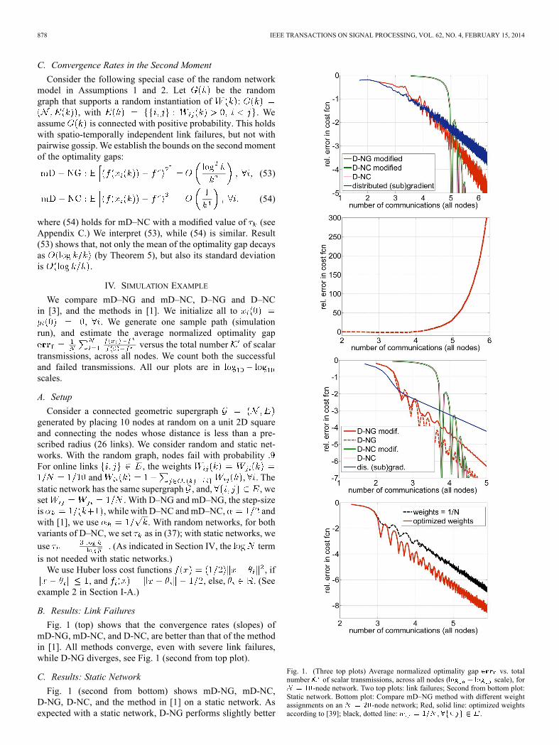
Fig. 1 (top) shows that the convergence rates (slopes) ofmD-NG, mD-NC, and D-NC, are better than that of the methodin [1]. All methods converge, even with severe link failures,while D-NG diverges, see Fig. 1 (second from top plot).

C. Results: Static Network

Fig. 1 (second from bottom) shows mD-NG, mD-NC,D-NG, D-NC, and the method in [1] on a static network. Asexpected with a static network, D-NG performs slightly better

Fig. 1. (Three top plots) Average normalized optimality gap vs. totalnumber of scalar transmissions, across all nodes ( scale), for

-node network. Two top plots: link failures; Second from bottom plot:Static network. Bottom plot: Compare mD–NG method with different weightassignments on an -node network; Red, solid line: optimized weightsaccording to [39]; black, dotted line: , .


than mD-NG, and both converge faster than [1]. D-NC andmD-NC perform similarly on both static and random networks.We also compared mD-NG and D-NG when mD-NG is runwith Metropolis weights , [41], while D-NG, because itrequires positive definite weights, is run with positive definite

. We report that D-NG performs margin-ally better than mD-NG (Figure omitted for brevity.)

D. Weight Optimization

Fig. 1 shows versus for uniform weights andthe optimized weights in [39] on a 20-node, 91-edge geometricgraph (radius ). Links fail independently in time and

space with probabilities . Here is the dis-tance between and . The losses are Huber :for nodes and for . The ’s are

as before. The two plots have the same rates (slopes). The op-timized weights lead to better convergence constant (agreeingwith Theorem 5), reducing the communication cost for the sameaccuracy.

V. CONCLUSION

We considered distributed optimization over random net-works where nodes minimize the sum of theirindividual convex costs. We model the random network bya sequence of independent, identically distributedrandom matrices that take values in the set of symmetric,stochastic matrices with positive diagonals. The ’s are convexand have Lipschitz continuous and bounded gradients. Wepresent mD–NG and mD–NC that are resilient to link failures.We establish their convergence in terms of the expected op-timality gap of the cost function at arbitrary node : mD–NGachieves rates and , where is thenumber of per-node gradient evaluations and is the numberof per-node communications; and mD–NC has ratesand , with arbitrarily small. Simulationexamples with link failures and Huber loss functions illustrateour findings.

APPENDIX

Proofs of Lemmas 1 and 6:Proof of Lemma 1: We prove (7). For ,

and (7) holds. Fix , . For matrix :. Applying this for , taking

expectation:

(55)

Next, following proofs in ([36], Section II-B):

Plugging this in (55), (7) follows. Next, (6) follows from (7) andJensen’s inequality. To prove (8), consider( by symmetry). By the independence of the ’s, the

sub-multiplicative property of norms, and taking expectation,obtain:

(56)

We applied (6) and (7) to get (56); thus, (8) for. If , , and the

result reduces to (7). The case , is symmetric.Finally, if , the result is trivial. The proofis complete.

Proof of Lemma 6: We prove (40). By (39), is theproduct of i.i.d. matrices that obey Assumptions 1 and2. Hence, by (7), obtain (40):

We prove (42). Let .For square matrices :

. Applying it times, obtain:

Using independence, taking expectation, and applying (40), ob-tain (42). By Jensen’s inequality, (41) follows from (42); rela-tion (43) is proved similarly.

Proofs of Lemmas 2 and 3:Proof of Lemma 2: Let be the derivative of .

Then (13) follows from:

To obtain (14), use (13) and :

Proof of Lemma 3: We prove Lemma 3 by first establishingtwo auxiliary results (Lemmas 9 and 10). Once these are estab-lished, we finish by proving Lemma 3.

Lemma 9 (Products ): Let , in (16),, , and:

(57)


Then, for , with and asbelow:

(58)

(59)

(60)

Proof: The proof is by mathematical induction on. Using , ,

and , it is easy to verify that the claim forholds, i.e.,

Now, suppose the claim holds for some fixed ,. Using the inductive hypothesis and the definition of:

(61)

(62)

Equality (61) uses , , , andthe fact that . (This is trivial toshow by mathematical induction on .) Next, recognize from(59)–(60) that ,and . Thus, the claimfor and the proof is complete.We establish bounds on the sums and .Lemma 10: Let and in (59)–(60),

, Then:

(63)

Proof: We prove each of the four inequalities above.Proof of the Right Inequality on : By induction on

. The claim holds for , since, . Let it be true for some .

For , write as:

(64)

Using (64) and the induction hypothesis:

Thus, the right inequality on .Proof of the Left Inequality on : Again, by induc-

tion on . The claim holds for , since:

Let the claim be true for some , i.e.,:

(65)

We show that Using (64):

where the last equality follows after algebraicmanipulations. Byinduction, the last inequality completes the proof of the lowerbound on .

Proof of Bounds on : The lower bound is trivial.The upper bound follows by induction. For :

Let the claim hold for some , i.e.,:From (59): Thus, by

the induction hypothesis:completing the proof of the upper bound on .

Proof of Lemma 3: We upper bound . Fixsome , , and consider in Lemma9. Note that . Thus,

(66)

By Lemma 10, the term:Using in (66) this equation, (by Lemma 10),

, and , get:

(67)for all , . Next, from (67), for

, , get:

We used and proved (17) for, for . To complete the proof, we show that (17)

holds also for: 1) , ; 2) , . Considerfirst case 1 and , .We have , and so (17) holdsfor , Next, consider case 2 and ,


. We have that , and so (17) alsoholds for , This proves the Lemma.

Proof of (53) – (54): Recall the random graph . Weassume that, for a certain connected graph with the Lapla-cian matrix , with probability . This,

with Assumption 1, implies :

by ([42], Lemma 11), can be taken as:Consider (35). Let

. Squaring (35), taking expectation, and bythe Cauchi-Schwarz inequality:

(68)

The first term in (68) is ; by Theorem 4, the secondis . Recall (29), let . Fix ,

. Let , and, for , and . From

(28) and , one can show(details omitted):

, and:

and so the third term in (68) is . Thus,

. Further, one can show

. Takingexpectation and applying Theorem 4, the result (53) follows.For mD–NC, prove (54) like (53) by letting .

REFERENCES[1] A. Nedic and A. Ozdaglar, “Distributed subgradient methods for multi-

agent optimization,” IEEE Trans. Autom. Control, vol. 54, no. 1, pp.48–61, Jan. 2009.

[2] J. Duchi, A. Agarwal, and M. Wainwright, “Dual averaging for dis-tributed optimization: Convergence and network scaling,” IEEE Trans.Autom. Control, vol. 57, no. 3, pp. 592–606, Mar. 2012.

[3] D. Jakovetic, J. Xavier, and J. M. F. Moura, “Fast distributed gradientmethods,” IEEE Trans. Autom. Control, 2014, to appear.

[4] C. Lopes and A. H. Sayed, “Adaptive estimation algorithms over dis-tributed networks,” presented at the 21st IEICE Signal Process. Symp.,Kyoto, Japan, Nov. 2006.

[5] F. Cattivelli and A. H. Sayed, “Diffusion LMS strategies for dis-tributed estimation,” IEEE Trans. Signal Process., vol. 58, no. 3, pp.1035–1048, Mar. 2010.

[6] S. Kar, J. M. F. Moura, and K. Ramanan, “Distributed parameter es-timation in sensor networks: Nonlinear observation models and im-perfect communication,” IEEE Trans. Inf. Theory, vol. 58, no. 6, pp.3575–3605, Jun. 2012.

[7] F. Cattivelli and A. H. Sayed, “Distributed detection over adaptive net-works using diffusion adaptation,” IEEE Trans. Signal Process., vol.59, no. 5, pp. 1917–1932, May 2011.

[8] D. Bajovic, D. Jakovetic, J. Xavier, B. Sinopoli, and J. M. F. Moura,“Distributed detection via Gaussian running consensus: Large devia-tions asymptotic analysis,” IEEE Trans. Signal Process., vol. 59, no. 9,pp. 4381–4396, Sep. 2011.

[9] A. H. Sayed, S.-Y. Tu, J. Chen, X. Zhao, and Z. Towfic, “Diffusionstrategies for adaptation and learning over networks,” IEEE SignalProcess. Mag., vol. 30, no. 3, pp. 155–171, May 2013.

[10] G. Mateos, J. A. Bazerque, and G. B. Giannakis, “Distributed sparselinear regression,” IEEE Trans. Signal Process., vol. 58, no. 11, pp.5262–5276, Nov. 2010.

[11] S. Boyd, N. Parikh, E. Chu, B. Peleato, and J. Eckstein, “Distributed op-timization and statistical learning via the alternating direction methodof multipliers,”Found. Trends in Mach. Learn., vol. 3, no. 1, pp. 1–122,2011.

[12] M. Rabbat and R. Nowak, “Distributed optimization in sensor net-works,” in Proc. 3rd Int. Symp. Inf. Process. in Sens. Netw. (IPSN),Berkeley, CA, Apr. 2004, pp. 20–27.

[13] D. Blatt and A. O. Hero, “Energy based sensor network source local-ization via projection onto convex sets (POCS),” IEEE Trans. SignalProcess., vol. 54, no. 9, pp. 3614–3619, 2006.

[14] D. Jakovetic, J. M. F. Moura, and J. Xavier, “Distributed Nesterov-likegradient algorithms,” in Proc. 51st IEEE Conf. Decision Contr. (CDC),Maui, HI, USA, Dec. 2012, pp. 5459–5464.

[15] D. Jakovetic, J. M. F. Moura, and J. Xavier, “Distributed Nesterov-like gradient algorithms,” in Proc. IEEE Asilomar Conf. Signals, Syst.,Comput., Pacific Grove, CA, USA, Nov. 2012, pp. 1513–1517.

[16] S. S. Ram, A. Nedic, and V. Veeravalli, “Asynchronous gossip algo-rithms for stochastic optimization,” in Proc. 48th IEEE Int. Conf. De-cision Control (CDC), Shanghai, China, Dec. 2009, pp. 3581–3586.

[17] I. Matei and J. S. Baras, “Performance evaluation of the consensus-based distributed subgradient method under random communicationtopologies,” IEEE J. Sel. Topics Signal Process., vol. 5, no. 4, pp.754–771, 2011.

[18] M. Zhu and S. Martínez, “On distributed convex optimization underinequality and equality constraints,” IEEE Trans. Autom. Control, vol.57, no. 1, pp. 151–164, Jan. 2012.

[19] J. A. Bazerque and G. B. Giannakis, “Distributed spectrum sensing forcognitive radio networks by exploiting sparsity,” IEEE Trans. SignalProcess., vol. 58, no. 3, pp. 1847–1862, Mar. 2010.

[20] J. Chen and A. H. Sayed, “Diffusion adaptation strategies for dis-tributed optimization and learning over networks,” IEEE Trans. SignalProcess., vol. 60, no. 8, pp. 4289–4305, Aug. 2012.

[21] S. Chouvardas, K. Slavakis, Y. Kopsinis, and S. Theodoridis, “Asparsity promoting adaptive algorithm for distributed learning,” IEEETrans. Signal Process., vol. 60, no. 10, pp. 5412–5425, Oct. 2012.

[22] L. Bottou and O. Bousquet, “The tradeoffs of large scale learning,” inAdvances in Neural Information Processing Systems, J. Platt, D. Koller,Y. Singer, and S. Roweis, Eds. La Jolla, CA, USA: Neural Inf. Pro-cessing Syst. Foundation/Salk Inst. for Biol. Studies-CNL, 2008, vol.20, pp. 161–168.

[23] S. Ram, A. Nedic, and V. Veeravalli, “Distributed stochastic subgra-dient projection algorithms for convex optimization,” J. Opt. TheoryAppl., vol. 147, no. 3, pp. 516–545, 2011.

[24] I. Lobel, A. Ozdaglar, and D. Feijer, “Distributed multi-agent opti-mization with state-dependent communication,” Math. Programm.,vol. 129, no. 2, pp. 255–284, 2011.

[25] I. Lobel and A. Ozdaglar, “Convergence analysis of distributed sub-gradient methods over random networks,” in Proc. 46th Ann. AllertonConf. Commun., Control, Comput., Monticello, IL, USA, Sep. 2008,pp. 353–360.

[26] B. Johansson, T. Keviczky, M. Johansson, and K. H. Johansson, “Sub-gradient methods and consensus algorithms for solving separable dis-tributed control problems,” in Proc. 47th IEEE Conf. Decision Control(CDC), Cancun, Mexico, Dec. 2008, pp. 4185–4190.

[27] K. Tsianos and M. Rabbat, “Distributed consensus and optimizationunder communication delays,” in Proc. 49th Allerton Conf. Commun.,Control, Comput., Monticello, IL, USA, Sep. 2011, pp. 974–982.

[28] I.-A. Chen and A. Ozdaglar, “A fast distributed proximal gradientmethod,” presented at the Allerton Conf. Commun., Control, Comput.,Monticello, IL, USA, Oct. 2012.

[29] D. Jakovetic, J. Xavier, and J. M. F. Moura, “Cooperative convex op-timization in networked systems: Augmented Lagrangian algorithmswith directed gossip communication,” IEEE Trans. Signal Process.,vol. 59, no. 8, pp. 3889–3902, Aug. 2011.

[30] J. Mota, J. Xavier, P. Aguiar, and M. Pueschel, “Distributed basis pur-suit,” IEEE Trans. Signal Process., vol. 60, no. 4, pp. 1942–1956, Apr.2011.


[31] U. V. Shanbhag, J. Koshal, and A. Nedic, “Multiuser optimization:Distributed algorithms and error analysis,” SIAM J. Control Optimiz.,vol. 21, no. 2, pp. 1046–1081, 2011.

[32] H. Terelius, U. Topcu, and R. M. Murray, “Decentralized multi-agentoptimization via dual decomposition,” presented at the 18th WorldCongr Int. Fed. Autom. Control (IFAC), Milano, Italy, Aug. 2011.

[33] I. D. Schizas, A. Ribeiro, and G. B. Giannakis, “Consensus in ad hocWSNs with noisy links—Part I: Distributed estimation of deterministicsignals,” IEEE Trans. Signal Process., vol. 56, no. 1, pp. 350–364, Jan.2009.

[34] F. Iutzeler, P. Bianchi, P. Ciblat, and W. Hachem, “Asynchronous dis-tributed optimization using a randomized alternating direction methodof multipliers,” in Proc. IEEE 52nd Conf. Decision Control (CDC),Florence, Italy, Dec. 2013, [Online].

[35] E.Wei andA. Ozdaglar, “On the convergence of asynchronousdistributed alternating direction method of multipliers,” ArXivpreprint, 2013 [Online]. Available: http://arxiv.org/abs/1307.8254

[36] S. Boyd, A. Ghosh, B. Prabhakar, and D. Shah, “Randomized gossipalgorithms,” IEEE Trans. Inf. Theory, vol. 52, no. 6, pp. 2508–2530,Jun. 2006.

[37] A. Dimakis, S. Kar, J. M. F. Moura, M. Rabbat, and A. Scaglione,“Gossip algorithms for distributed signal processing,” Proc. IEEE, vol.98, no. 11, pp. 1847–1864, 2010.

[38] Y. E. Nesterov, “A method for solving the convex programmingproblem with convergence rate ,” (in Russian) Dokl. Akad.Nauk SSSR, vol. 269, pp. 543–547, 1983.

[39] D. Jakovetić, J. Xavier, and J. M. F. Moura, “Weight optimizationfor consensus algorithms with correlated switching topology,” IEEETrans. Signal Process., vol. 58, no. 7, pp. 3788–3801, Jul. 2010.

[40] A. Tahbaz-Salehi and A. Jadbabaie, “On consensus in randomnetworks,” in Proc. 44th Annu. Allerton Conf. Commun., Control,Comput., Allerton House, IL, USA, Sep. 2006, pp. 1315–1321.

[41] L. Xiao, S. Boyd, and S. Lall, “A scheme for robust distributed sensorfusion based on average consensus,” in Proc. Inf. Process. Sens. Netw.(IPSN), Los Angeles, CA, 2005, pp. 63–70.

[42] D. Bajovic, J. Xavier, J. M. F. Moura, and B. Sinopoli, “Consensusand products of random stochastic matrices: Exact rate for conver-gence in probability,” IEEE Trans. Signal Process., vol. 61, no. 10, pp.2557–2571, May 2013.

Dušan Jakovetić (S’10–M’14) received the dipl.ing. diploma from the School of Electrical Engi-neering, University of Belgrade, in August 2007,and the Ph.D. degree in electrical and computerengineering from Carnegie Mellon University,Pittsburgh, PA, and Instituto de Sistemas e Robótica(ISR), Instituto Superior Técnico (IST), Lisbon,Portugal, in May 2013.Since October 2013, he has been a research

fellow at the BioSense Center, University of NoviSad, Serbia. From June to September 2013, he was

a postdoctoral researcher at IST. His research interests include distributedinference and distributed optimization.

João Manuel Freitas Xavier (S’97–M’03) receivedthe Ph.D. degree in electrical and computer engi-neering from the Instituto Superior Técnico (IST),Lisbon, Portugal, in 2002.Currently, he is an Assistant Professor in the De-

partment of Electrical and Computer Engineering,IST. He is also a Researcher at the Institute ofSystems and Robotics (ISR), Lisbon, Portugal. Hiscurrent research interests are in the area of optimiza-tion and statistical inference for distributed systems.

José M. F. Moura (S’71–M’75–SM’90–F’94)received the engenheiro electrotécnico degree fromInstituto Superior Técnico (IST), Lisbon, Portugal,and the M.Sc., E.E., and D.Sc. degrees in EECSfrom MIT, Cambridge, MA.During 2013-2014, he is a visiting Professor at

New York University (NYU) and at CUSP-NYU onsabbatical leave from Carnegie Mellon University(CMU), Pittsburgh, PA, where he is the Philip andMarsha Dowd University Professor. Previously, hewas on the faculty at IST and was visiting Professor

at MIT. He is founding director of ICTI@CMU, a large education and researchprogram between CMU and Portugal, www.cmuportugal.org. His research in-terests include statistical, algebraic, and distributed signal and image processingand signal processing on graphs. He has published more than 470 papers, has10 patents issued by the US Patent Office, and cofounded SpiralGen.Dr. Moura was the IEEEDivision IX Director and member of the IEEEBoard

of Directors (2012–13) and has served on several IEEE Boards. He was Presi-dent (2008–2009) of the IEEE Signal Processing Society(SPS), served as Editorin Chief for the IEEE TRANSACTIONS IN SIGNAL PROCESSING, interim Editor inChief for the IEEE SIGNAL PROCESSING LETTERS, and member of several Ed-itorial Boards, including the IEEE PROCEEDINGS, IEEE SIGNAL PROCESSINGMAGAZINE, and the ACM Transactions on Sensor Networks. He is memberof the US National Academy of Engineering, corresponding member of theAcademy of Sciences of Portugal, Fellow of the AAAS. He received the IEEESignal Processing Society Technical Achievement Award and the IEEE SignalProcessing Society Award.

868 IEEE TRANSACTIONS ON SIGNAL PROCESSING, VOL. 62, NO. …

Documents

Transcript of 868 IEEE TRANSACTIONS ON SIGNAL PROCESSING, VOL. 62, NO. …