IEEE TRANSACTIONS ON SIGNAL PROCESSING, VOL. 62, NO. 20 ...

IEEE TRANSACTIONS ON SIGNAL PROCESSING, VOL. 62, NO. 20, OCTOBER 15, 2014 5471

A Comprehensive Approach to Universal PiecewiseNonlinear Regression Based on Trees

N. Denizcan Vanli and Suleyman Serdar Kozat, Senior Member, IEEE

Abstract—In this paper, we investigate adaptive nonlinearregression and introduce tree based piecewise linear regressionalgorithms that are highly efficient and provide significantlyimproved performance with guaranteed upper bounds in anindividual sequence manner. We use a tree notion in order topartition the space of regressors in a nested structure. The intro-duced algorithms adapt not only their regression functions butalso the complete tree structure while achieving the performanceof the “best” linear mixture of a doubly exponential numberof partitions, with a computational complexity only polynomialin the number of nodes of the tree. While constructing thesealgorithms, we also avoid using any artificial “weighting” ofmodels (with highly data dependent parameters) and, instead,directly minimize the final regression error, which is the ultimateperformance goal. The introduced methods are generic such thatthey can readily incorporate different tree construction methodssuch as random trees in their framework and can use differentregressor or partitioning functions as demonstrated in the paper.

Index Terms—Nonlinear regression, nonlinear adaptive fil-tering, binary tree, universal, adaptive.

I. INTRODUCTION

N ONLINEAR adaptive filtering and regression are ex-tensively investigated in the signal processing [1]–[19]

and machine learning literatures [20]–[23], especially forapplications where linear modeling [24], [25] is inadequate,hence, does not provide satisfactory results due to the structuralconstraint on linearity. Although nonlinear approaches can bemore powerful than linear methods in modeling, they usuallysuffer from overfitting, stability and convergence issues [1],[26]–[28], which considerably limit their application to signalprocessing problems. These issues are especially exacerbatedin adaptive filtering due to the presence of feedback, whichis even hard to control for linear models [26], [27], [29].Furthermore, for applications involving big data, which requireto process input vectors with considerably large dimensions,nonlinear models are usually avoided due to unmanageablecomputational complexity increase [30]. To overcome thesedifficulties, “tree” based nonlinear adaptive filters or regressors

Manuscript received July 24, 2013; revised December 23, 2013; acceptedAugust 14, 2014. Date of publication August 20, 2014; date of current versionSeptember 16, 2014. The associate editor coordinating the review of this man-uscript and approving it for publication was Dr. Slawomir Stanczak. This workwas supported in part by the IBMFaculty Award and in part by TUBITAK underContract 112E161 and Contract 113E517.The authors are with the Department of Electrical and Electronics En-

gineering, Bilkent University, Bilkent, Ankara 06800, Turkey (e-mail:[email protected]; [email protected]).Color versions of one or more of the figures in this paper are available online

at http://ieeexplore.ieee.org.Digital Object Identifier 10.1109/TSP.2014.2349882

Fig. 1. The partitioning of a two dimensional regressor space using a completetree of depth-2 with hyperplanes for separation. The whole regressor space isfirst bisected by , which is defined by the hyperplane , where the regionon the direction of vector corresponds to the child with “1” label. We thencontinue to bisect children regions using and , defined by and ,respectively.

are introduced as elegant alternatives to linear models sincethese highly efficient methods retain the breadth of nonlinearmodels while mitigating the overfitting and convergence issues[2], [4], [30]–[33].In its most basic form, a regression tree defines a hierarchical

or nested partitioning of the regressor space [2]. As an example,consider the binary tree in Fig. 1, which partitions a two di-mensional regressor space. On this tree, each node representsa bisection of the regressor space, e.g., using hyperplanes forseparation, resulting a complete nested and disjoint partitionof the regressor space. After the nested partitioning is defined,the structure of the regressors in each region can be chosen asdesired, e.g., one can assign a linear regressor in each regionyielding an overall piecewise linear regressor. In this sense, treebased regression is a natural nonlinear extension to linear mod-eling, in which the space of regressors is partitioned into a unionof disjoint regions where a different regressor is trained. Thisnested architecture not only provides an efficient and tractablestructure, but also is shown to easily accommodate to the in-trinsic dimension of data, naturally alleviating the overfittingissues [30], [34].Although nonlinear regressors using decision trees are pow-

erful and efficient tools for modeling, there exist several algo-rithmic preferences and design choices that affect their perfor-mance in real life applications [2], [4], [31]. Especially their

1053-587X © 2014 IEEE. Personal use is permitted, but republication/redistribution requires IEEE permission.See http://www.ieee.org/publications_standards/publications/rights/index.html for more information.

5472 IEEE TRANSACTIONS ON SIGNAL PROCESSING, VOL. 62, NO. 20, OCTOBER 15, 2014

Fig. 2. All different partitions of the regressor space that can be obtained usinga depth-2 tree. Any of these partition can be used to construct a piecewise linearmodel, which can be adaptively trained to minimize the regression error. Thesepartitions are based on the separation functions shown in Fig. 1.

adaptive learning performance may greatly suffer if the algo-rithmic parameters are not tuned carefully, which is particu-larly hard to accommodate for applications involving nonsta-tionary data exhibiting saturation effects, threshold phenomenaor chaotic behavior [4]. In particular, the success of the treebased regressors heavily depends on the “careful” partitioningof the regressor space. Selection of a good partition, includingits depth and regions, from the hierarchy is essential to balancethe bias and variance of the regressor [30], [34]. As an example,even for a uniform binary tree, while increasing the depth ofthe tree improves the modeling power, such an increase usu-ally results in overfitting [4]. There exist numerous approachesthat provide “good” partitioning of the regressor space that areshown to yield satisfactory results on the average under certainstatistical assumptions on the data or on the application [30].We note that on the other extreme, there exist methods in

adaptive filtering and computational learning theory, whichavoid such a direct commitment to a particular partitioning butinstead construct a weighted average of all possible piecewisemodels defined on a tree [4], [35], [36]. Note that a full binarytree of depth- , as shown in Fig. 1 for , with hardseparation boundaries, defines a doubly exponential number[37] of complete partition of the regressor space (see Fig. 2).Each such partitioning of the regressor space is representedby the collection of the nodes of the full tree where each nodeis assigned to a particular region of the regressor space. Anyof these partitions can be used to construct and then train apiecewise linear or nonlinear regressor. Instead of fixing one ofthese partitions, one can run all the models (or subtrees) in par-allel and combine the final outputs based on their performance.Such approaches are shown to mitigate the bias variance tradeoff in a deterministic framework [4], [35], [36]. However, thesemethods are naturally constraint to work on a specific tree orpartitionings, i.e., the tree is fixed and cannot be adapted tothe data, and the weighting among the models usually have notheoretical justifications (although they may be inspired frominformation theoretic considerations [38]). As an example, the“universal weighting” coefficients in [4], [24], [39]–[41] or

the exponentially weighted performance measure are definedbased on algorithmic concerns and provide universal bounds,however, do not minimize the final regression error. In partic-ular, the performance of these methods highly depends on theseweighting coefficients and algorithmic parameters that shouldbe tuned to the particular application for successful operation[4], [31].To this end, we provide a comprehensive solution to nonlinear

regression using decision trees. In this paper, we introduce al-gorithms that are shown i) to be highly efficient ii) to providesignificantly improved performance over the state of the art ap-proaches in different applications iii) to have guaranteed per-formance bounds without any statistical assumptions. Our al-gorithms not only adapt the corresponding regressors in eachregion, but also learn the corresponding region boundaries, aswell as the “best” linear mixture of a doubly exponential numberof partitions to minimize the final estimation or regression error.We introduce algorithms that are guaranteed to achieve the per-formance of the best linear combination of a doubly exponen-tial number of models with a significantly reduced computa-tional complexity. The introduced approaches significantly out-perform [4], [24], [39] based on trees in different applications inour examples, since we avoid any artificial weighting of modelswith highly data dependent parameters and, instead, “directly”minimize the final error, which is the ultimate performance goal.Our methods are generic such that they can readily incorporaterandom projection (RP) or -d trees in their framework as com-mented in our simulations, e.g., the RP trees can be used as thestarting partitioning to adaptively learn the tree, regressors andweighting to minimize the final error as data progress.In this paper, we first introduce an algorithm that asymptoti-

cally achieves the performance of the “best” linear combinationof a doubly exponential number of different models that canbe represented by a depth- tree a with fixed regressor spacepartitioning with a computational complexity only linear in thenumber of nodes of the tree.We then provide a guaranteed upperbound on the performance of this algorithm and prove that asthe data length increases, this algorithm achieves the perfor-mance of the “best” linear combination of a doubly exponentialnumber of models without any statistical assumptions. Further-more, even though we refrain from any statistical assumptionson the underlying data, we also provide the mean squared per-formance of this algorithm compared to the mean squared per-formance of the best linear combination of the mixture. Thesemethods are generic and truly sequential such that they do notneed any a priori information, e.g., upper bounds on the data[2], [4], (such upper bounds does not hold in general, e.g., forGaussian data). Although the combination weights in [4], [35],[36] are artificially constraint to be positive and sum up to 1[42], we have no such restrictions and directly adapt to the datawithout any constraints. We then extend these results and pro-vide the final algorithm (with a slightly increased computationalcomplexity), which “adaptively” learns also the correspondingregions of the tree to minimize the final regression error. Thisapproach learns i) the “structure” of the tree, ii) the regressors ineach region, and iii) the linear combination weights to merge allpossible partitions, to minimize the final regression error. In thissense, this algorithm can readily capture the salient characteris-tics of the underlying data while avoiding bias to a particularmodel or structure.

VANLI AND KOZAT: A COMPREHENSIVE APPROACH TO UNIVERSAL PIECEWISE NONLINEAR REGRESSION BASED ON TREES 5473

In Section III, we first present an algorithm with a fixed re-gressor space partitioning and present a guaranteed upper boundon its performance. We then significantly reduce the compu-tational complexity of this algorithm using the tree structure.In Section IV, we extend these results and present the final al-gorithm that adaptively learns the tree structure, region bound-aries, region regressors and combination weights to minimizethe final regression error. We then demonstrate the performanceof our algorithms through simulations in Section V. We then fi-nalize our paper with concluding remarks.

II. PROBLEM DESCRIPTION

In this paper, all vectors are column vectors and denoted byboldface lower case letters. Matrices are represented by bold-face uppercase letters. For a vector is the-norm, where is the ordinary transpose. Here, repre-

sents a dimensional identity matrix.We study sequential nonlinear regression, where we observe

a desired signal , and regression vectors, such that we sequentially estimate by

and is an adaptive nonlinear regression function. At eachtime , the regression error is given by

Although there exist several different approaches to select thecorresponding nonlinear regression function, we particularlyuse piecewise models such that the space of the regression vec-tors, i.e., , is adaptively partitioned using hyperplanesbased on a tree structure. We also use adaptive linear regressorsin each region. However, our framework can be generalizedto any partitioning of the regression space, i.e., not necessarilyusing hyperplanes, such as using [30], or any regression func-tion in each region, i.e., not necessarily linear. Furthermore,both the region boundaries as well as the regressors in eachregion are adaptive.

A. A Specific Partition on a Tree

To clarify the framework, suppose the corresponding spaceof regressor vectors is two dimensional, i.e., , and wepartition this regressor space using a depth-2 tree as in Fig. 1.A depth-2 tree is represented by three separating functions

and , which are defined using three hyperplanes with di-rection vectors and , respectively (See Fig. 1). Dueto the tree structure, three separating hyperplanes generate onlyfour regions, where each region is assigned to a leaf on the treegiven in Fig. 1 such that the partitioning is defined in a hierar-chical manner, i.e., is first processed by and then by

. A complete tree defines a doubly exponential number,, of subtrees each of which can also be used to partition

the space of past regressors. As an example, a depth-2 tree de-fines 5 different subtrees or partitions as shown in Fig. 2, whereeach of these subtrees is constructed using the leaves and thenodes of the original tree. Note that a node of the tree representsa region which is the union of regions assigned to its left andright children nodes [38].The corresponding separating (indicator) functions can be

hard, e.g., if the data falls into the region pointed by the

direction vector , and otherwise. Without loss of gen-erality, the regions pointed by the direction vector are labeledas “1” regions on the tree in Fig. 1. The separating functions canalso be soft. As an example, we use the logistic regression clas-sifier [43]

(1)

as the soft separating function, where is the direction vectorand is the offset, describing a hyperplane in the -dimen-sional regressor space. With an abuse of notation we combinethe direction vector with the offset parameter and denoteit by . Then the separator function in (1) can berewritten as

(2)

where . One can easily use other differentiable softseparating functions in this setup in a straightforward manner asremarked later in the paper.To each region, we assign a regression function to generate

an estimate of . For a depth-2 (or a depth- ) tree, there are 7(or ) nodes (including the leaves) and 7 (or )regions corresponding to these nodes, where the combination ofthese nodes or regions form a complete partition. In this paper,we assign linear regressors to each region. For instance considerthe third model in Fig. 2, i.e., , where this partition is theunion of 4 regions each corresponding to a leaf of the originalcomplete tree in Fig. 1, labeled as 00, 01, 10, and 11. Thedefines a complete partitioning of the regressor space, hencecan be used to construct a piecewise linear regressor. At eachregion, say the 00th region, we generate the estimate

(3)

where is the linear regressor vector assigned toregion 00. Considering the hierarchical structure of the tree andhaving calculated the region estimates, the final estimate ofis given by

(4)

for any . We emphasize that any can be usedin a similar fashion to construct a piecewise linear regressor.Continuing with the specific partition , we adaptively train

the region boundaries and regressors to minimize the final re-gression error. As an example, if we use a stochastic gradientdescent algorithm [42], [44]–[46], we update the regressor ofthe node “00” as

where is the step size to update the region regressors. Sim-ilarly, region regressors can be updated for all regions

. Separator functions can also be trained using thesame approach, e.g., the separating function of the node 0, ,can be updated as


where is the step size to update the separator functions and

(5)

according to the separator function in (2). Other separating func-tions (different than the logistic regressor classifier) can also betrained in a similar fashion by simply calculating the gradientwith respect to the extended direction vector and plugging in(5).Until now a specific partition, i.e., , is used to construct

a piecewise linear regressor, although the tree can represent. However, since the data structure is unknown, one

may not prefer a particular model [4], [35], [36], i.e., there maynot be a specific best model or the best model can change intime. As an example, the simpler models, e.g., , may performbetter while there is not sufficient data at the start of trainingand the finer models, e.g., , can recover through the learningprocess. Hence, we hypothetically construct all doubly expo-nential number of piecewise linear regressors corresponding toall partitions (see Fig. 2) and then calculate an adaptive linearcombination of the outputs of all, while these algorithms learnthe region boundaries as well as the regressors in each region.In Section III, we first consider the scenario in which the re-

gressor space is partitioned using hard separator functions andcombine different models for a depth- tree with a com-putational complexity . In Section IV, we partition theregressor space with soft separator functions and adaptively up-date the region boundaries to achieve the best partitioning ofthe -dimensional regressor space with a computational com-plexity .

III. REGRESSOR SPACE PARTITIONING VIA HARDSEPARATOR FUNCTIONS

In this section, we consider the regression problem in whichthe sequential regressors (as described in Section II.A) for allpartitions in the doubly exponential tree class are combinedwhen hard separation functions are used, i.e., . Inthis section, the hard boundaries are not trained, however, boththe regressors of each region and the combination parameters tomerge the outputs of all partitions are trained. To partition theregressor space, we first construct a tree with an arbitrary depth,say a tree of depth- , and denote the number of different modelsof this class by , e.g., one can use RP trees as thestarting tree [30]. While the th model (i.e., partition) gen-erates the regression output at time for all ,we linearly combine these estimates using the weighting vector

such that the final estimate of our al-gorithm at time is given as

(6)

where . The regression error at time iscalculated as

For different models that are embedded within a depth- tree,we introduce an algorithm (given in Algorithm 1) that asymptot-ically achieves the same cumulative squared regression error asthe optimal linear combination of these models without any sta-tistical assumptions. This algorithm is constructed in the proofof the following theorem and the computational complexity ofthe algorithm is only linear in the number of the nodes of thetree.Theorem 1: Let and be arbitrary, bounded,

and real-valued sequences. The algorithm given in Algorithm1 when applied to these data sequence yields

(7)

for all , when is strongly convex , where, and are the estimates of

at time for .This theorem implies that our algorithm (given in Algorithm

1), asymptotically achieves the performance of the best combi-nation of the outputs of different models that can be rep-resented using a depth- tree with a computational complexity

. Note that as given in Algorithm 1, no a priori informa-tion, e.g., upper bounds, on the data is used to construct the algo-rithm. Furthermore, the algorithm can use different regressors,e.g., [4], or regions seperation functions, e.g., [30], to define thetree.Assuming that the constituent partition regressors converge

to stationary distributions, such as for Gaussian regressors, andunder widely used separation assumptions [26], [47] such thatthe expectation of , and are separable,we have the following theorem.Theorem 2: Assuming that the partition regressors, i.e.,

, and converge to zero mean stationary distri-butions, we have

where is the learning rate of the stochastic gradient update,

for the algorithm (given in Algorithm 1).Theorem 2 directly follows Chapter 6 of [26] since we use a

stochastic gradient algorithm to merge the partition regressors[26], [47]. Hence, the introduced algorithmmay also achieve themean square error performance of the best linear combinationof the constituent piecewise regressors if is selected carefully.

A. Proof of Theorem 1 and Construction of Algorithm 1

To construct the final algorithm, we first introduce a “di-rect” algorithmwhich achieves the corresponding bound in The-orem 1. This direct algorithm has a computational complexity

since one needs to calculate the correlation informationof models to achieve the performance of the best linearcombination. We then introduce a specific labeling technique


and using the properties of tree structure, construct an algo-rithm to obtain the same upper bound as the “direct” algorithm,yet with a significantly smaller computational complexity, i.e.,

.For a depth- tree, suppose , are obtained

as described in Section II.A. To achieve the upper bound in (7),we use the stochastic gradient descent approach and update thecombination weights as

(8)

where is the step-size parameter (or the learning rate) of thegradient descent algorithm. We first derive an upper bound onthe sequential learning regret , which is defined as

where is the optimal weight vector over , i.e.,

Following [44], using Taylor series approximation, for somepoint on the line segment connecting to , we have

(9)

According to the update rule in (8), at each iteration the updateon weights are performed as . Hence,we have

Then we obtain

(10)

Under the mild assumptions that for someand is -strong convex for some [44], we

achieve the following upper bound

(11)

By selecting and summing up the regret terms in(11), we get

Note that (8) achieves the performance of the best linear combi-nation of piecewise linear models that are defined by thetree. However, in this form (8) requires a computational com-plexity of since the vector has a size of . Wenext illustrate an algorithm that performs the same adaptation in(8) with a complexity of .We next introduce a labeling for the tree nodes following [38].

The root node is labeled with an empty binary string and as-suming that a node has a label , where is a binary string, welabel its upper and lower children as and , respectively.Here we emphasize that a string can only take its letters fromthe binary alphabet , where 0 refers to the lower child, and1 refers to the upper child of a node. We also introduce anotherconcept, i.e., the definition of the prefix of a string. We say thata string is a prefix to string ifand for all , and the empty string is aprefix to all strings. Let represent all prefixes to the string, i.e., , where is the length ofthe string is the string with , and isthe empty string, such that the first letters of the stringforms the string for .We then observe that the final estimate of any model can be

found as the combination of the regressors of its leaf nodes.According to the region has fallen, the final estimate will becalculated with the separator functions. As an example, for thesecond model in Fig. 2 (i.e., partition), say , andhard separator functions are used. Then the final estimate of thismodel will be given as . For any separator function,the final estimate of the desired data at time of the thmodel,i.e., can be obtained according to the hierarchical structureof the tree as the sum of regressors of its leaf nodes, each ofwhich are scaled by the values of the separator functions of thenodes between the leaf node and the root node. Hence, we cancompactly write the final estimate of the th model at time as

(12)

where is the set of all leaf nodes in the th model, isthe regressor of the node is the length of the string

is the prefix to string with length is the thletter of the string , i.e., , and finally denotesthe separator function at node such that


with defined as in (2). We emphasize that we dropped -de-pendency of and to simplify notation.As an example, if we consider the third model in Fig. 2 as

the th model (i.e., ), where , thenwe can calculate the final estimate of that model as follows

(13)

Note that (4) and (13) are the same special cases of (12).We next denote the product terms in (12) as follows

(14)

to simplify the notation. Here, can be viewed as the estimateof the node (i.e., region) given that for some ,where denotes all leaf nodes of the depth- tree class, i.e.,

. Then (12) can be rewritten as follows

Since we now have a compact form to represent the tree andthe outputs of each partition, we next introduce a method to cal-culate the combination weights of piecewise regressoroutputs in a simplified manner.To this end, we assign a particular linear weight to each node.

We denote the weight of node at time as and then wedefine the weight of the th model as the sum of weights of itsleaf nodes, i.e.,

for all . Since the weight of eachmodel, saymodel, is recursively updated as

we achieve the following recursive update on the node weights

(15)

where is defined as in (14).This result implies that instead of managing memory

locations, and making calculations, only keeping trackof the weights of every node is sufficient, and the number ofnodes in a depth- model is , where denotesthe set of all nodes in a depth- tree. As an example, forwe obtain . Therefore we can re-duce the storage and computational complexity from to

by performing the update in (15) for all . We then

continue the discussion with the update of weights performed ateach time when hard separator functions are used.Without loss of generality assume that at time , the regression

vector has fallen into the region specified by the node. Consider the node regressor defined in (14) for some

node . Since we are using hard separator functions, weobtain

where represents all prefixes to the string , i.e.,. Then at each time we only update the weights

of the nodes , hence we only makeupdates since the hard separation functions are used for parti-tioning of the regressor space.Before stating the algorithm that combines these node

weights as well as node estimates, and generates the same finalestimate as in (6) with a significantly reduced computationalcomplexity, we observe that for a node with length

, there exist a total of

different models in which the node is a leaf node of thatmodel, where and for all . For

case, i.e., for , one can clearly observe that thereexists only one model having as the leaf node, i.e., the modelhaving no partitions, therefore .Having stated how to store all estimates and weights in

memory locations, and perform the updates at each iteration, wenow introduce an algorithm to combine them in order to obtainthe final estimate of our algorithm, i.e., . We empha-size that the sizes of the vectors and are , whichforces us to make computations. We however introducean algorithm with a complexity of that is able to achievethe exact same result.

Algorithm 1: Decision Fixed Tree (DFT) Regressor

1: for to do2:3:4: for all do5:

6:7: for all do8:

9:10: end for11:12: end for13:14: for all do15:

16:17: end for18: end for


For a depth- tree, at time say for a node .Then the final estimate of our algorithm is found by

(16)

where is the set of all leaf nodes inmodel , andis the longest prefix to the string in the th model, i.e.,

. Let denote the set of allprefixes to string . We then observe that the regressors of thenodes will be sufficient to obtain the final estimateof our algorithm. Therefore, we only consider the estimates of

nodes.In order to further simplify the final estimate in (16), we first

let , i.e., denotes the setof all nodes of a depth- tree, whose set of prefixes include thenode . As an example, for a depth-2 tree, we have

. We then define a function for arbitrary twonodes , as the number of models having both andas its leaf nodes. Trivially, if , then . If

, then letting denote the longest prefix to both and ,i.e., the longest string in , we obtain

(17)

Since from the definition of the tree, wenaturally have .Now turning our attention back to (16) and considering the

definition in (17), we notice that the number of occurrences ofthe product in is given by . Hence, the com-bination weight of the estimate of the node at time can becalculated as follows

(18)

Then, the final estimate of our algorithm becomes

(19)

We emphasize that the estimate of our algorithm given in (19)achieves the exact same result with with a computa-tional complexity of . Hence, the proof is concluded.

IV. REGRESSOR SPACE PARTITIONING VIA ADAPTIVE SOFTSEPARATOR FUNCTIONS

In this section, the sequential regressors (as described inSection II.A) for all partitions in the doubly exponential tree

class are combined when soft separation functions are used,i.e., , where is the extendedregressor vector and is the extended direction vector. Byusing soft separator functions, we train the correspondingregion boundaries, i.e., the structure of the tree.As in Section III, for different models that are embedded

within a depth- tree, we introduce the algorithm (given inAlgorithm 2) achieving asymptotically the same cumulativesquared regression error as the optimal combination of the bestadaptive models. The algorithm is constructed in the proof ofthe Theorem 3.The computational complexity of the algorithm of Theorem

3 is whereas it achieves the performance of the bestcombination of different “adaptive” regressors that par-titions the -dimensional regressor space. The computationalcomplexity of the first algorithm was , however, it wasunable to learn the region boundaries of the regressor space. Inthis case since we are using soft separator functions, we need toconsider the cross-correlation of every node estimate and nodeweight, whereas in the previous case there we were only con-sidering the cross-correlation of the estimates of the prefixesof the node such that and the weights ofevery node. This change transforms the computational com-plexity from to . Moreover, for all inner nodesa soft separator function is defined. In order to update the re-gion boundaries of the partitions, we have to update the direc-tion vector of size since . Therefore, consideringthe cross-correlation of the final estimates of every node, we geta computational complexity of .Theorem 3: Let and be arbitrary, bounded,

and real-valued sequences. The algorithm given in Algorithm2 when applied these sequences yields

(20)

for all , when is strongly convex , whereand represents the estimate

of at time for the adaptive model .This theorem implies that our algorithm (given in Algorithm

2), asymptotically achieves the performance of the best linearcombination of the different adaptive models that canbe represented using a depth- tree with a computational com-plexity . We emphasize that while constructing the al-gorithm, we refrain from any statistical assumptions on the un-derlying data, and our algorithm works for any sequence of

with an arbitrary length of . Furthermore, one canuse this algorithm to learn the region boundaries and then feedthis information to the first algorithm to reduce computationalcomplexity.

A. Outline of the Proof of Theorem 3 and Construction ofAlgorithm 2

The proof of the upper bound in Theorem 3 follows similarlines to the proof of upper bound in Theorem 1, therefore isomitted. In this proof, we provide the detailed algorithmicdescription and highlight the computational complexitydifferences.


According to the same labeling operation we presented inSection II, the final estimate of the th model at time can befound as follows

Similarly, the weight of the th model is given by

Since we use soft separator functions, we have andwithout introducing any approximations, the final estimate ofour algorithm is given as follows

Here, we observe that for arbitrary two nodes , theproduct appears times in , where isthe number of models having both and as its leaf nodes (aswe previously defined in (17)). Hence, according to the notationderived in (17) and (18), we obtain the final estimate of ouralgorithm as follows

(21)

Note that (21) is equal to with a computationalcomplexity of .Unlike Section III, in which each model has a fixed parti-

tioning of the regressor space, here, we define the regressormodels with adaptive partitions. For this, we use a stochasticgradient descent update

(22)

for all nodes , where is the learning rate of theregion boundaries and is the derivative ofwith respect to . After some algebra, we obtain

(23)

where we use the logistic regression classifier as our separatorfunction, i.e., . Therefore, we have

(24)

Algorithm 2: Decision Adaptive Tree (DAT) Regressor

1: for to do2:3: for all do4:5: end for6: for all do7:8:9: for to do10:11: end for12:13:14: for all do15:16:17: end for18:19: end for20:21: for all do22:23:24: end for25: for all do26:27: for all do

28:29: end for30: for all do

31:32: end for33:34: end for35: end for

Note that other separator functions can also be used in a similarway by simply calculating the gradient with respect to the ex-tended direction vector and plugging in (23) and (24).We emphasize that includes the product of and

terms, hence in order not to slow down the learningrate of our algorithm, we may restrict forsome . According to this restriction, we define theseparator functions as follows

According to the update rule in (23), the computational com-plexity of the introduced algorithm results in . Thisconcludes the outline of the proof and the construction of thealgorithm.

B. Selection of the Learning Rates

We emphasize that the learning rate can be set accordingto the similar studies in the literature [26], [44] or considering


the application requirements. However, for the introduced al-gorithm to work smoothly, we expect the region boundaries toconverge faster than the node weights, therefore, we conven-tionally choose the learning rate to update the region bound-aries as . Experimentally, we observedthat different choices of also yields acceptable performance,however, we note that when updating , we have the multi-plication term , which significantly decreases thesteps taken at each time . Therefore, in order to compensate forit, such a selection is reasonable.On the other hand, for stability purposes, one can consider to

put an upper bound on the steps at each time . When is suffi-ciently away from the region boundaries , it is either close toor . However, when falls right on a region boundary,

we have , which results in an approximately 25 timesgreater step than the expected one, when . This issueis further exacerbated when falls on the boundary of multipleregion crossings, e.g., say when we have the fourquadrants as the four regions (leaf nodes) of the depth-2 tree. Insuch a scenario, one can observe a times greater step thanexpected, which may significantly perturb the stability of the al-gorithm. That is why, two alternate solutions can be proposed: 1)a reasonable threshold (e.g., )) over the steps canbe embedded when is small (or equivalently, a regularizationconstant can be embedded), 2) can be sufficiently increasedaccording to the depth of the tree. Throughout the experiments,we used the first approach.

C. Selection of the Depth of the Tree

In many real life applications, we do not know how the truedata is generated, therefore, the accurate selection of the depthof the decision tree is usually a difficult problem. For instance,if the desired data is generated from a piecewise linear model,then in order for the conventional approaches that use a fixedtree structure (i.e., fixed partitioning of the regressor space) toperfectly estimate the data, they need to perfectly guess the un-derlying partitions in hindsight. Otherwise, in order to capturethe salient characteristics of the desired data, the depth of thetree should be increased to infinity. Hence, the performance ofsuch algorithms significantly varies according to the initial par-titioning of the regressor space, which makes it harder to decidehow to select the depth of the tree.On the other hand, the introduced algorithm adapts its region

boundaries to minimize the final regression error. Therefore,even if the initial partitioning of the regressor space is not accu-rate, our algorithm will learn to the locally optimal partitioningof the regressor space for any given depth . In this sense, onecan select the depth of the decision tree by only considering thecomputational complexity issues of the application.

V. SIMULATIONS

In this section, we illustrate the performance of our al-gorithms under different scenarios with respect to variousmethods. We first consider the regression of a signal generatedby a piecewise linear model when the underlying partition ofthe model corresponds to one of the partitions represented bythe tree. We then consider the case when the partitioning doesnot match any partition represented by the tree to demonstratethe region-learning performance of the introduced algorithm.

We also illustrate the performance of our algorithms in underfit-ting and overfitting (in terms of the depth of the tree) scenarios.We then consider the prediction of two benchmark chaoticprocesses: the Lorenz attractor and the Henon map. Finally, weillustrate the merits of our algorithm using benchmark data sets(both real and synthetic) such as California housing [48]–[50],elevators [48], kinematics [49], pumadyn [49], and bank [50](which will be explained in detail in Subsection V.F).Throughout this section, “DFT” represents the decision fixed

tree regressor (i.e., Algorithm 1) and “DAT” represents thedecision adaptive tree regressor (i.e., Algorithm 2). Similarly,“CTW” represents the context tree weighting algorithm of [4],“OBR” represents the optimal batch regressor, “VF” representsthe truncated Volterra filter [5], “LF” represents the simplelinear filter, “B-SAF” and “CR-SAF” represent the Beizerand the Catmul-Rom spline adaptive filter of [6], respectively,“FNF” and “EMFNF” represent the Fourier and even mirrorFourier nonlinear filter of [7], respectively. Finally, “GKR”represents the Gaussian-Kernel regressor and it is constructedusing node regressors, say , and a fixed Gaussianmixture weighting (that is selected according to the underlyingsequence in hindsight), giving

where and

for all .For a fair performance comparison, in the corresponding

experiments in Subsections V.E and V.F, the desired data andthe regressor vectors are normalized between since thesatisfactory performance of the several algorithms require theknowledge on the upper bounds (such as the B-SAF and theCR-SAF) and some require these upper bounds to be between

(such as the FNF and the EMFNF). Moreover, in thecorresponding experiments in Subsections V.B, V.C, and V.D,the desired data and the regressor vectors are normalizedbetween for the VF, the FNF, and the EMFNF dueto the aforementioned reason. The regression errors of thesealgorithms are then scaled back to their original values for afair comparison.Considering the illustrated examples in the respective papers

[4], [6], [7], the orders of the FNF and the EMFNF are set to3 for the experiments in Subsections V.B, V.C, and V.D, 2 forthe experiments in Subsection V.E, and 1 for the experimentsin Subsection V.F. The order of the VF is set to 2 for all experi-ments, except for the California housing experiment, in which itis set to 3. Similarly, the depth of the tree of the DAT algorithmis set to 2 for all experiments, except for the California housingexperiment, in which it is set to 3. The depths of the trees of theDFT and the CTW algorithms are set to 2 for all experiments.For the tree based algorithms, the regressor space is initially par-titioned by the direction vectors for all

nodes , where if ,e.g., when , we have the four quadrants as thefour leaf nodes of the tree. Finally, we used cubic B-SAF andCR-SAF algorithms, whose number of knots are set to 21 for all


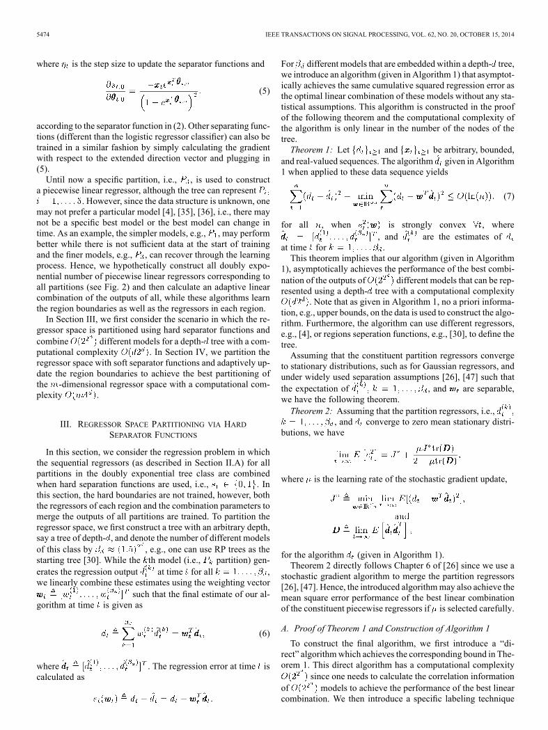
TABLE ICOMPARISON OF THE COMPUTATIONAL COMPLEXITIES OF THE PROPOSEDALGORITHMS. IN THE TABLE, REPRESENTS THE DIMENSIONALITY OFTHE REGRESSOR SPACE, REPRESENTS THE DEPTH OF THE TREES INTHE RESPECTIVE ALGORITHMS, AND REPRESENTS THE ORDER OF THE

CORRESPONDING FILTERS AND ALGORITHMS

experiments. We emphasize that both these parameters and thelearning rates of these algorithms are selected to give equal rateof performance and convergence.

A. Computational Complexities

As can be observed from Table I, among the tree based algo-rithms that partition the regressor space, the CTW algorithm hasthe smallest complexity since at each time , it only associatesthe regressor vector with nodes (the leaf node hasfallen into and all its prefixes) and their individual weights. TheDFT algorithm also considers the same nodes on the tree,but in addition, it calculates the weight of the each node with re-spect to the rest of the nodes, i.e., it correlates nodes withall the nodes. The DAT algorithm, however, estimates thedata with respect to the correlation of all the nodes, one another,which results in a computational complexity of . In orderfor the Gaussian-Kernel Regressor (GKR) to achieve a compa-rable nonlinear modeling power, it should have mass points,which results in a computational complexity of .On the other hand, the filters such as the VF, the FNF, and

the EMFNF introduce the nonlinearity by directly consideringthe th (and up to th) powers of the entries of the regressorvector. In many practical applications, such methods cannot beapplied due to the high dimensionality of the regressor space.Therefore, the algorithms such as the B-SAF and the CR-SAFare introduced to decrease the high computational complexity ofsuch approaches. However, as can be observed from our simula-tion results, the introduced algorithm significantly outperformsits competitors in various benchmark problems.The algorithms such as the VF, the FNF, and the EMFNF

have more than enough number of basis functions, which resultin a significantly slower and parameter dependent convergenceperformance with respect to the other algorithms. On the otherhand, the performances of the algorithms such as the B-SAF,the CR-SAF, and the CTW algorithm are highly dependent onthe underlying setting that generates the desired signal. Fur-thermore, for all these algorithms to yield satisfactory results,prior knowledge on the desired signals and the regressor vec-tors is needed. The introduced algorithms, on the other hand,do not rely on any prior knowledge, and still outperform theircompetitors.

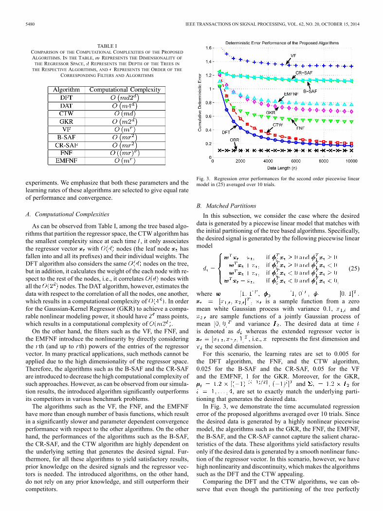
Fig. 3. Regression error performances for the second order piecewise linearmodel in (25) averaged over 10 trials.

B. Matched Partitions

In this subsection, we consider the case where the desireddata is generated by a piecewise linear model that matches withthe initial partitioning of the tree based algorithms. Specifically,the desired signal is generated by the following piecewise linearmodel

(25)

whereis a sample function from a zero

mean white Gaussian process with variance 0.1, andare sample functions of a jointly Gaussian process of

mean and variance . The desired data at timeis denoted as whereas the extended regressor vector is

, i.e., represents the first dimension andthe second dimension.For this scenario, the learning rates are set to 0.005 for

the DFT algorithm, the FNF, and the CTW algorithm,0.025 for the B-SAF and the CR-SAF, 0.05 for the VFand the EMFNF, 1 for the GKR. Moreover, for the GKR,

and for, are set to exactly match the underlying parti-

tioning that generates the desired data.In Fig. 3, we demonstrate the time accumulated regression

error of the proposed algorithms averaged over 10 trials. Sincethe desired data is generated by a highly nonlinear piecewisemodel, the algorithms such as the GKR, the FNF, the EMFNF,the B-SAF, and the CR-SAF cannot capture the salient charac-teristics of the data. These algorithms yield satisfactory resultsonly if the desired data is generated by a smooth nonlinear func-tion of the regressor vector. In this scenario, however, we havehigh nonlinearity and discontinuity, whichmakes the algorithmssuch as the DFT and the CTW appealing.Comparing the DFT and the CTW algorithms, we can ob-

serve that even though the partitioning of the tree perfectly


Fig. 4. Progress of (a) the model weights and (b) the node weights averaged over 10 trials for the DFT algorithm. Note that the model weights do not sum up to 1.

matches with the underlying partition in (25), the learningperformance of the DFT algorithm significantly outperformsthe CTW algorithm especially for short data records. Ascommented in the text, this is expected since the context-treeweighting method enforces the sum of the model weights to be1, however, the introduced algorithms have no such restrictions.As seen in Fig. 4(a), the model weights sum up to 2.1604 in-stead of 1. Moreover, in the CTW algorithm all model weightsare “forced” to be nonnegative whereas in our algorithm modelweights can also be negative as seen in Fig. 4(a). In Fig. 4(b),the individual node weights are presented. We observe that thenodes (i.e., regions) that directly match with the underlyingpartition that generates the desired data have higher weightswhereas the weights of the other nodes decrease. We also pointout that although the tree based algorithms [4], [35], [36] need apriori information, such as an upper bound on the desired data,for a successful operation, whereas the introduced algorithmhas no such requirements.

C. Mismatched Partitions

In this subsection, we consider the case where the desired datais generated by a piecewise linear model that mismatches withthe initial partitioning of the tree based algorithms. Specifically,the desired signal is generated by the following piecewise linearmodel

(26)

whereis a sample function from a

zero mean white Gaussian process with variance 0.1, andare sample functions of a jointly Gaussian process of meanand variance . The learning rates are set to 0.005 for

the DFT, the DAT, and the CTW algorithms, 0.1 for the FNF,0.025 for the B-SAF and the CR-SAF, 0.05 for the EMFNF andthe VF. Moreover, in order to match the underlying partition,

Fig. 5. Regression error performances for the second order piecewise linearmodel in (26).

the mass points of the GKR are set to, and

with the same covariance matrixin the previous example.Fig. 5 shows the normalized time accumulated regression

error of the proposed algorithms. We emphasize that the DATalgorithm achieves a better error performance compared to itscompetitors. Comparing Figs. 3 and 5, one can observe thedegradation in the performances of the DFT and the CTW al-gorithms. This shows the importance of the initial partitioningof the regressor space for tree based algorithms to yield asatisfactory performance. Comparing the same figures, one canalso observe that the rest of the algorithms performs almostsimilar to the previous scenario.The DFT and the CTW algorithms converge to the best batch

regressor having the predetermined leaf nodes (i.e., the bestregressor having the four quadrants of two dimensional space


Fig. 6. Changes in the boundaries of the leaf nodes of the depth-2 tree of the DAT algorithm for . The separator functionsadaptively learn the boundaries of the piecewise linear model in (26).

Fig. 7. Progress of the node weights for the piecewise linear model in (26) for (a) the DFT algorithm and (b) the DAT algorithm.

as its leaf nodes). However that regressor is sub-optimal sincethe underlying data is generated using another constellation,hence their time accumulated regression error is always lowerbounded by compared to the global optimal regressor. TheDAT algorithm, on the other hand, adapts its region boundariesand captures the underlying unevenly rotated and shifted re-gressor space partitioning, perfectly. Fig. 6 shows how our al-gorithm updates its separator functions and illustrates the non-linear modeling power of the introduced DAT algorithm.

We also present the node weights for the DFT and the DATalgorithms in Fig. 7(a) and (b), respectively. In Fig. 7(a), wecan observe that the DFT algorithm cannot estimate the under-lying data accurately, hence its node weights show unstable be-havior. On the other hand, as can be observed from Fig. 7(b),the DAT algorithm learns the optimal node weights as the re-gion boundaries are learned. In this manner, the DAT algorithmachieves a significantly superior performance with respect to itscompetitors.


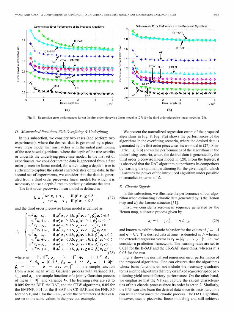
Fig. 8. Regression error performances for (a) the first order piecewise linear model in (27) (b) the third order piecewise linear model in (28).

D. Mismatched Partitions With Overfitting & Underfitting

In this subsection, we consider two cases (and perform twoexperiments), where the desired data is generated by a piece-wise linear model that mismatches with the initial partitioningof the tree based algorithms, where the depth of the tree overfitsor underfits the underlying piecewise model. In the first set ofexperiments, we consider that the data is generated from a firstorder piecewise linear model, for which using a depth-1 tree issufficient to capture the salient characteristics of the data. In thesecond set of experiments, we consider that the data is gener-ated from a third order piecewise linear model, for which it isnecessary to use a depth-3 tree to perfectly estimate the data.The first order piecewise linear model is defined as

(27)

and the third order piecewise linear model is defined as

(28)where

is a sample functionfrom a zero mean white Gaussian process with variance 0.1,

and are sample functions of a jointly Gaussian processof mean and variance . The learning rates are set to0.005 for the DFT, the DAT, and the CTW algorithms, 0.05 forthe EMFNF, 0.01 for the B-SAF, the CR-SAF, and the FNF, 0.5for the VF, and 1 for the GKR, where the parameters of the GKRare set to the same values in the previous example.

We present the normalized regression errors of the proposedalgorithms in Fig. 8. Fig. 8(a) shows the performances of thealgorithms in the overfitting scenario, where the desired data isgenerated by the first order piecewise linear model in (27). Sim-ilarly, Fig. 8(b) shows the performances of the algorithms in theunderfitting scenario, where the desired data is generated by thethird order piecewise linear model in (28). From the figures, itis observed that the DAT algorithm outperforms its competitorsby learning the optimal partitioning for the given depth, whichillustrates the power of the introduced algorithm under possiblemismatches in terms of .

E. Chaotic Signals

In this subsection, we illustrate the performance of our algo-rithm when estimating a chaotic data generated by i) the Henonmap and ii) the Lorenz attractor [51].First, we consider a zero-mean sequence generated by the

Henon map, a chaotic process given by

(29)

and known to exhibit chaotic behavior for the values ofand . The desired data at time is denoted as whereasthe extended regressor vector is , i.e., weconsider a prediction framework. The learning rates are set to0.025 for the B-SAF and the CR-SAF algorithms, whereas it is0.05 for the rest.Fig. 9 shows the normalized regression error performance of

the proposed algorithms. One can observe that the algorithmswhose basis functions do not include the necessary quadraticterms and the algorithms that rely on a fixed regressor space par-titioning yield unsatisfactory performance. On the other hand,we emphasize that the VF can capture the salient characteris-tics of this chaotic process since its order is set to 2. Similarly,the FNF can also learn the desired data since its basis functionscan well approximate the chaotic process. The DAT algorithm,however, uses a piecewise linear modeling and still achieves


Fig. 9. Regression error performances of the proposed algorithms for thechaotic process presented in (29).

the asymptotically same performance as the VF, while outper-forming the FNF algorithm.Second, we consider the chaotic signal set generated using

the Lorenz attractor [51] that is defined by the following threediscrete time equations:

(30)

(31)

(32)

where we set , and to gen-erate the well-known chaotic solution of the Lorenz attractor.In the experiment, is selected as the desired data and the twodimensional region represented by is set as the regressorspace, that is, we try to estimate with respect to and .The learning rates are set to 0.01 for all the algorithms.Fig. 10 illustrates the nonlinear modeling power of the DAT

algorithm even when estimating a highly nonlinear chaoticsignal set. As can be observed from Fig. 10, the DAT algo-rithm significantly outperforms its competitors and achieves asuperior error performance since it tunes its region boundariesto the optimal partitioning of the regressor space, whereasthe performances of the other algorithms directly rely on theinitial selection of the basis functions and/or tree structures andpartitioning.

F. Benchmark Real and Synthetic Data

In this subsection, we first consider the regression of abenchmark real-life problem that can be found in many dataset repositories such as [48]–[50]: California housing—esti-mation of the median house prices in the California area usingCalifornia housing database. In this experiment, the learningrates are set to 0.01 for all the algorithms. Fig. 11 providesthe normalized regression errors of the proposed algorithms,where it is observed that the DAT algorithm outperforms itscompetitors and can achieve a much higher nonlinear modelingpower with respect to the rest of the algorithms.

Fig. 10. Regression error performances for the chaotic signal generated fromthe Lorenz attractor in (30), (31), and (32) with parameters

, and .

Fig. 11. Regression error performances for the real data set: Californiahousing—estimation of the median house prices in the California area usingCalifornia housing database [48]–[50].

Aside from the California housing data set, we also considerthe regression of several benchmark real life and synthetic datafrom the corresponding data set repositories:• Kinematics [48] —a realistic simulation of theforward dynamics of an 8 link all-revolute robot arm. Thetask in all data sets is to predict the distance of the end-effector from a target. (among the existent variants of thisdata set, we used the variant with , which is knownto be highly nonlinear and medium noisy).

• Elevators [49] —obtained from the task of con-trolling a F16 aircraft. In this case the goal variable is re-lated to an action taken on the elevators of the aircraft.

• Pumadyn [49] —a realistic simulation of thedynamics of Unimation Puma 560 robot arm. The task inthe data set is to predict the angular acceleration of one ofthe robot arm’s links.


TABLE IITIME ACCUMULATED NORMALIZED ERRORS OF THE PROPOSED ALGORITHMS. EACH DIMENSION OF THE DATA SETS IS NORMALIZED BETWEEN

• Bank [50] —generated from a simplistic simu-lator, which simulates the queues in a series of banks. Tasksare based on predicting the fraction of bank customers wholeave the bank because of full queues (among the existentvariants of this data set, we used the variant with ).

The learning rates of the LF, the VF, the FNF, the EMFNF,and the DAT algorithm are set to , whereas it is set to 10 forthe B-SAF and the CR-SAF algorithms, where for thekinematics, the elevators, and the bank data sets andfor the pumadyn data set. In Table II, it is observed that the per-formance of the DAT algorithm is superior to its competitorssince it achieves a much higher nonlinear modeling power withrespect to the rest of the algorithms. Furthermore, the DAT algo-rithm achieves this superior performance with a computationalcomplexity that is only linear in the regressor space dimension-ality. Hence, the introduced algorithm can be used in real lifebig data problems.

VI. CONCLUDING REMARKS

We study nonlinear regression of deterministic signals usingtrees, where the space of regressors is partitioned using a nestedtree structure where separate regressors are assigned to each re-gion. In this framework, we introduce tree based regressors thatboth adapt their regressors in each region as well as their treestructure to best match to the underlying data while asymptoti-cally achieving the performance of the best linear combinationof a doubly exponential number of piecewise regressors rep-resented on a tree. As shown in the text, we achieve this per-formance with a computational complexity only linear in thenumber of nodes of the tree. Furthermore, the introduced al-gorithms do not require a priori information on the data suchas upper bounds or the length of the signal. Since these algo-rithms directly minimize the final regression error and avoidusing any artificial weighting coefficients, they readily outper-form different tree based regressors in our examples. The in-troduced algorithms are generic such that one can easily usedifferent regressor or separation functions or incorporate par-titioning methods such as the RP trees in their framework asexplained in the paper.

REFERENCES[1] A. C. Singer, G. W. Wornell, and A. V. Oppenheim, “Nonlinear au-

toregressive modeling and estimation in the presence of noise,” Digit.Signal Process., vol. 4, no. 4, pp. 207–221, 1994.

[2] O. J. J. Michel, A. O. Hero, and A.-E. Badel, “Tree-structured nonlinearsignal modeling and prediction,” IEEE Trans. Signal Process., vol. 47,no. 11, pp. 3027–3041, 1999.

[3] R. J. Drost and A. C. Singer, “Constrained complexity generalized con-text-tree algorithms,” in Proc. IEEE/SP 14th Workshop Statist. SignalProcess., 2007, pp. 131–135.

[4] S. S. Kozat, A. C. Singer, and G. C. Zeitler, “Universal piecewise linearprediction via context trees,” IEEE Trans. Signal Process., vol. 55, no.7, pp. 3730–3745, 2007.

[5] M. Schetzen, The Volterra and Wiener Theories of Nonlinear Sys-tems. New York, NY, USA: Wiley, 1980.

[6] M. Scarpiniti, D. Comminiello, R. Parisi, and A. Uncini, “Nonlinearspline adaptive filtering,” Signal Process., vol. 93, no. 4, pp. 772–783,2013.

[7] A. Carini and G. L. Sicuranza, “Fourier nonlinear filters,” SignalProcess., vol. 94, no. 0, pp. 183–194, 2014.

[8] V. Kekatos and G. Giannakis, “Sparse Volterra and polynomial re-gression models: Recoverability and estimation,” IEEE Trans. SignalProcess., vol. 59, no. 12, pp. 5907–5920, 2011.

[9] L. Montefusco, D. Lazzaro, and S. Papi, “Fast sparse image reconstruc-tion using adaptive nonlinear filtering,” IEEE Trans. Image Process.,vol. 20, no. 2, pp. 534–544, 2011.

[10] Q. Zhu, Z. Zhang, Z. Song, Y. Xie, and L. Wang, “A novel nonlinearregression approach for efficient and accurate image matting,” IEEESignal Process. Lett., vol. 20, no. 11, pp. 1078–1081, 2013.

[11] R. Mittelman and E. Miller, “Nonlinear filtering using a new proposaldistribution and the improved fast Gauss transform with tighter per-formance bounds,” IEEE Trans. Signal Process., vol. 56, no. 12, pp.5746–5757, 2008.

[12] L. Montefusco, D. Lazzaro, and S. Papi, “Nonlinear filtering for sparsesignal recovery from incomplete measurements,” IEEE Trans. SignalProcess., vol. 57, no. 7, pp. 2494–2502, 2009.

[13] W. Zhang, B.-S. Chen, and C.-S. Tseng, “Robust filtering for non-linear stochastic systems,” IEEE Trans. Signal Process., vol. 53, no. 2,pp. 589–598, 2005.

[14] H. Zhao and J. Zhang, “A novel adaptive nonlinear filter-basedpipelined feedforward second-order Volterra architecture,” IEEETrans. Signal Process., vol. 57, no. 1, pp. 237–246, 2009.

[15] L. Ma, Z. Wang, J. Hu, Y. Bo, and Z. Guo, “Robust variance-con-strained filtering for a class of nonlinear stochastic systems withmissingmeasurements,” Signal Process., vol. 90, no. 6, pp. 2060–2071,2010.

[16] W. Yang, M. Liu, and P. Shi, “ filtering for nonlinear stochasticsystems with sensor saturation, quantization and random packetlosses,” Signal Process., vol. 92, no. 6, pp. 1387–1396, 2012.

[17] W. Li and Y. Jia, “H-infinity filtering for a class of nonlinear discrete-time systems based on unscented transform,” Signal Process., vol. 90,no. 12, pp. 3301–3307, 2010.

[18] S. Wen, Z. Zeng, and T. Huang, “Reliable filtering for neutralsystems with mixed delays and multiplicative noises,” Signal Process.,vol. 94, no. 0, pp. 23–32, 2014.

[19] M. F. Huber, “Chebyshev polynomial Kalman filter,” Digit. SignalProcess., vol. 23, no. 5, pp. 1620–1629, 2013.

[20] D. P. Helmbold and R. E. Schapire, “Predicting nearly as well as thebest pruning of a decision tree,”Mach. Learn., vol. 27, no. 1, pp. 51–68,1997.

[21] O.-A. Maillard and R. Munos, “Linear regression with random projec-tions,” J. Mach. Learn. Res., vol. 13, pp. 2735–2772, 2012.

[22] R. Rosipal and L. J. Trejo, “Kernel partial least squares regression inreproducing Kernel Hilbert Space,” J. Mach. Learn. Res., vol. 2, pp.97–123, 2001.

[23] O.-A. Maillard and R. Munos, “Some greedy learning algorithms forsparse regression and classification with Mercer kernels,” J. Mach.Learn. Res., vol. 13, pp. 2735–2772, 2012.

[24] A. C. Singer and M. Feder, “Universal linear prediction by modelorder weighting,” IEEE Trans. Signal Process., vol. 47, no. 10, pp.2685–2699, 1999.

[25] T. Moon and T. Weissman, “Universal FIR MMSE filtering,” IEEETrans. Signal Process., vol. 57, no. 3, pp. 1068–1083, 2009.

[26] A. H. Sayed, Fundamentals of Adaptive Filtering. Hoboken, NJ,USA: Wiley, 2003.

[27] V. H. Nascimento and A. H. Sayed, “On the learning mechanismof adaptive filters,” IEEE Trans. Signal Process., vol. 48, no. 6, pp.1609–1625, 2000.


[28] T. Y. Al-Naffouri and A. H. Sayed, “Transient analysis of adaptivefilters with error nonlinearities,” IEEE Trans. Signal Process., vol. 51,no. 3, pp. 653–663, 2003.

[29] J. Arenas-Garcia, A. R. Figueiras-Vidal, and A. H. Sayed,“Mean-square performance of a convex combination of two adaptivefilters,” IEEE Trans. Signal Process., vol. 54, no. 3, pp. 1078–1090,2006.

[30] S. Dasgupta and Y. Freund, “Random projection trees for vector quan-tization,” IEEE Trans. Inf. Theory, vol. 55, no. 7, pp. 3229–3242, 2009.

[31] Y. Yilmaz and S. S. Kozat, “Competitive randomized nonlinear pre-diction under additive noise,” IEEE Signal Process. Lett., vol. 17, no.4, pp. 335–339, 2010.

[32] G. David and A. Averbuch, “Hierarchical data organization, clusteringand denoising via localized diffusion folders,” Appl. Comput. Harmon.Anal., vol. 33, no. 1, pp. 1–23, 2012.

[33] N. B. Lee, A. B. , and L. Wasserman, “Treelets—An adaptive multi-scale basis for sparse unordered data,” Ann. Appl. Statist., vol. 2, no. 2,pp. 435–471, 2008.

[34] J. L. Bentley, “Multidimensional binary search trees in database appli-cations,” IEEE Trans. Softw. Eng., vol. SE-5, no. 4, pp. 333–340, 1979.

[35] E. Takimoto, A. Maruoka, and V. Vovk, “Predicting nearly as wellas the best pruning of a decision tree through dyanamic programmingscheme,” Theoretic. Comput. Sci., vol. 261, pp. 179–209, 2001.

[36] E. Takimoto and M. K. Warmuth, “Predicting nearly as well as the bestpruning of a planar decision graph,” Theoretic. Comput. Sci., vol. 288,pp. 217–235, 2002.

[37] A. V. Aho and N. J. A. Sloane, “Some doubly exponential sequences,”Fibonacci Quart., vol. 11, pp. 429–437, 1970.

[38] F. M. J. Willems, Y. M. Shtarkov, and T. J. Tjalkens, “The context-treeweighting method: Basic properties,” IEEE Trans. Inf. Theory, vol. 41,no. 3, pp. 653–664, 1995.

[39] A. C. Singer, S. S. Kozat, and M. Feder, “Universal linear least squaresprediction: Upper and lower bounds,” IEEE Trans. Inf. Theory, vol. 48,no. 8, pp. 2354–2362, 2002.

[40] T. Linder and G. Lagosi, “A zero-delay sequential scheme for lossycoding of individual sequences,” IEEE Trans. Inf. Theory, vol. 47, no.6, pp. 2533–2538, 2001.

[41] A. Gyorgy, T. Linder, and G. Lugosi, “Efficient adaptive algorithmsand minimax bounds for zero-delay lossy source coding,” IEEE Trans.Signal Process., vol. 52, no. 8, pp. 2337–2347, 2004.

[42] J. Arenas-Garcia, V. Gomez-Verdejo, and A. R. Figueiras-Vidal,“New algorithms for improved adaptive convex combination of LMStransversal filters,” IEEE Trans. Instrum. Meas., vol. 54, no. 6, pp.2239–2249, 2005.

[43] D. W. Hosmer, S. Lemeshow, and R. X. Sturdivant, Applied LogisticRegression. Hoboken, NJ, USA: Wiley, 2013.

[44] E. Hazan, A. Agarwal, and S. Kale, “Logarithmic regret algorithmsfor online convex optimization,” Mach. Learn., vol. 69, no. 2–3, pp.169–192, 2007.

[45] E. Eweda, “Comparison of RLS, LMS, and sign algorithms for trackingrandomly time-varying channels,” IEEE Trans. Signal Process., vol.42, no. 11, pp. 2937–2944, 1994.

[46] J. Arenas-Garcia, M. Martinez-Ramon, V. Gomez-Verdejo, and A. R.Figueiras-Vidal, “Multiple plant identifier via adaptive LMS convexcombination,” in Proc. IEEE Int. Symp. Intell. Signal Process., 2003,pp. 137–142.

[47] S. S. Kozat, A. T. Erdogan, A. C. Singer, and A. H. Sayed, “Steadystate MSE performance analysis of mixture approaches to adaptive fil-tering,” IEEE Trans. Signal Process., vol. 58, no. 8, pp. 4050–4063,Aug. 2010.

[48] C. E. Rasmussen, R. M. Neal, G. Hinton, D. Camp, M. Revow, Z.Ghahramani, R. Kustra, and R. Tibshirani, Delve Data Sets [Online].Available: [Online]. Available: http://www.cs.toronto.edu/delve/data/datasets.html

[49] J. Alcala-Fdez, A. Fernandez, J. Luengo, J. Derrac, S. Garca, L. Snchez,and F. Herrera, “KEEL data-mining software tool: Data set reposi-tory, integration of algorithms and experimental analysis framework,”J. Multiple-Valued Logic Soft Comput., vol. 17, no. 2–3, pp. 255–287,2011.

[50] L. Torgo, Regression Data Sets [Online]. Available: [Online]. Avail-able: http://www.dcc.fc.up.pt/ltorgo/Regression/DataSets.html

[51] E. N. Lorenz, “Deterministic nonperiodic flow,” J. Atmosph. Sci., vol.20, no. 2, pp. 130–141, 1963.

N. Denizcan Vanli was born in Nigde, Turkey, in1990. He received the B.S. degree with high honorsin electrical and electronics engineering from BilkentUniversity, Ankara, Turkey, in 2013.He is currently working toward the M.S. degree

in the Department of Electrical and ElectronicsEngineering at Bilkent University. His research in-terests include sequential learning, adaptive filtering,machine learning, and statistical signal processing.

Suleyman Serdar Kozat (A’10–M’11–SM’11) re-ceived the B.S. degree with full scholarship and highhonors from Bilkent University, Turkey. He receivedthe M.S. and Ph.D. degrees in electrical and com-puter engineering from University of Illinois at Ur-bana Champaign, Urbana, IL. Dr. Kozat is a graduateof Ankara Fen Lisesi.After graduation, Dr. Kozat joined IBM Research,

T. J. Watson Research Lab, Yorktown, NewYork, USas a Research Staff Member in the Pervasive SpeechTechnologies Group. While doing his Ph.D., he was

also working as a Research Associate at Microsoft Research, Redmond, Wash-ington, US in the Cryptography and Anti-Piracy Group. He holds several patentinventions due to his research accomplishments at IBM Research andMicrosoftResearch. After serving as an Assistant Professor at Koc University, Dr. Kozatis currently an Assistant Professor (with the Associate Professor degree) at theElectrical And Electronics Department of Bilkent University.Dr. Kozat is the President of the IEEE Signal Processing Society, Turkey

Chapter. He has been elected to the IEEE Signal Processing Theory andMethods Technical Committee and IEEE Machine Learning for Signal Pro-cessing Technical Committee, 2013. He has been awarded IBM Faculty Awardby IBM Research in 2011, Outstanding Faculty Award by Koc Universityin 2011 (granted the first time in 16 years), Outstanding Young ResearcherAward by the Turkish National Academy of Sciences in 2010, ODTU Prof.Dr. Mustafa N. Parlar Research Encouragement Award in 2011, OutstandingFaculty Award by Bilim Kahramanlari, 2013 and holds Career Award by theScientific Research Council of Turkey, 2009.

IEEE TRANSACTIONS ON SIGNAL PROCESSING, VOL. 62, NO. 20 ...

Documents

Transcript of IEEE TRANSACTIONS ON SIGNAL PROCESSING, VOL. 62, NO. 20 ...