82 JOURNAL OF INTERNET ENGINEERING, VOL. 1, NO....

82 JOURNAL OF INTERNET ENGINEERING, VOL. 1, NO. 2, OCTOBER 2007

A Theory of Load Adjustments and

its Implications for Congestion ControlSergey Gorinsky, Manfred Georg, Maxim Podlesny, and Christoph Jechlitschek

Abstract—Multiplicative Increase (MI), Additive Increase (AI),and Multiplicative Decrease (MD) are linear adjustments usedextensively in networking. However, their properties are not fullyunderstood. We analyze responsiveness (time for the total loadto reach the target load), smoothness (maximal size of the totalload oscillations after reaching the target load), fairing speed(speed of convergence to equal individual loads) and scalabili-ties of MAIMD (Multiplicative Additive Increase MultiplicativeDecrease) algorithms, which generalize AIMD algorithms viaoptional inclusion of MI. We prove that an MAIMD can providefaster asymptotic fairing than a less smooth AIMD. Furthermore,we discover that loads under a specific MAIMD converge fromany initial state to the same periodic pattern, called a canonicalcycle. While imperfectly correlated with smoothness, the canon-ical cycle reliably predicts the asymptotic fairing speed. We alsoshow that AIMD algorithms offer the best trade-off betweensmoothness and responsiveness. Then, we introduce smoothness-responsiveness diagrams to investigate MAIMD scalabilities.Finally, we discuss implications of the theory for the practiceof congestion control.

Index Terms–Congestion control, linear adjustments, fairingspeed, smoothness, responsiveness, scalability.

I. INTRODUCTION

To regulate network congestion, Transmission Control Pro-

tocol (TCP) [1] and numerous other protocols rely on linear

adjustments such as Multiplicative Increase (MI), Additive

Increase (AI), and Multiplicative Decrease (MD) [10]. Linear

adjustments are also extensively used for various networking

tasks beyond traditional congestion control, e.g., for load

balancing in clustered servers [32], active queue manage-

ment [11], wireless media access [16], and multicast group

subscription [9]. Despite the wide adoption of linear adjust-

ments, their properties still require further understanding.

In this paper, we advance such comprehension by analyzing

linear adjustment algorithms in the classical Chiu-Jain model

where distributed users adjust their loads on a shared resource

in response to uniform binary feedback that indicates whether

the total load exceeds a target [10]. The original analysis [10]

examined linear adjustment algorithms with respect to several

interesting properties including responsiveness (time for the

total load to reach the target), smoothness (maximal size of

the total load oscillations after reaching the target), and fairing

(convergence to equal individual loads). Chiu and Jain showed

that MAIMD (Multiplicative Additive Increase Multiplicative

Decrease) algorithms which generalize AIMD via optional

inclusion of MI are stable, i.e., provide convergence to the

target total load and equal individual loads. By revealing that

the AIMD subclass of MAIMD algorithms offers the fastest

fairing after a single adjustment, the original analysis supplied

Manuscript received November 17, 2006.This work was performed at the Applied Research Laboratory, Depart-

ment of Computer Science and Engineering, Washington University in St.Louis, One Brookings Drive, St. Louis, MO 63130-4899, USA by SergeyGorinsky ([email protected]), Manfred Georg ([email protected]),Maxim Podlesny ([email protected]), and Christoph Jechlitschek([email protected]).

a theoretical justification for using AIMD in TCP congestion

avoidance [17]. Chiu and Jain also showed that an overall op-

timal MAIMD algorithm does not exist due to a fundamental

trade-off between responsiveness and smoothness.

Our choice of the model warrants an early discussion due

to the following concerns about Chiu-Jain model: 1) The

model makes oversimplifying assumptions. For instance, it

assumes uniform feedback to all users while measurements at

backbone routers show independent packet loss [6] and thus

support an alternative assumption of non-uniform feedback;

moreover, whereas MIMD control does not converge to equal

individual loads in Chiu-Jain model, MIMD is fair in models

with non-uniform feedback [3], [14]. Also, Chiu-Jain model

implies that traffic consists of only long-lived flows, which is

an obvious deviation from the Internet reality; 2) The model

is not universal even in the context of congestion control.

In particular, due to the assumption of binary feedback, the

model does not lend itself to analysis of eXplicit Control

Protocol (XCP) [20] and other designs where routers provide

richer explicit feedback about congestion; 3) Chiu-Jain model

is almost two decades old. Since then, more elaborate models

have appeared and led to new insights and designs [2], [4], [7],

[12], [21], [25]–[27]. Nevertheless, we believe that Chiu-Jain

model is appropriate for our investigation for the following

reasons of increasing importance:

• Wide applicability. Chiu-Jain model represents many

real scenarios with sufficient accuracy. The assumption of

binary feedback does not interfere with analyzing TCP,

which remains the dominant Internet transport protocol,

or more recent proposals such as Scalable Transmission

Control Protocol (STCP) [22] and Variable-structure con-

gestion Control Protocol (VCP) [33], which does not infer

congestion from losses but instead relies on explicit router

feedback. Uniform feedback is generally unrealistic but

does occur in real networks where congestion at a low-

multiplexing access link affects all local flows [31].

• Elegance and intuitiveness. The model is elegant in for-

mulation and offers clear interpretation of derived results.

More elaborate models become complex and lose intu-

itive appeal without eliminating all unrealistic assump-

tions. Lack of simple credible analysis [13] contributes

greatly to the Internet ossification [5] because complex

models fail to persuade a critical mass of stakeholders in

overall goodness of advocated innovations [18]. Although

Katabi, Handley, and Rohrs [20] proved XCP fairing in

a more complicated model, they supported the argument

with analogies between XCP and AIMD. The references

to AIMD (which is widely known as stable in Chiu-Jain

model) helped to alleviate concerns about XCP stability

and promote the overall positive reception of XCP, even

though XCP does not actually use AIMD but performs

nonlinear adjustments which depend on not only the

current load and fixed coefficients (as in Chiu-Jain model)

GORINSKY et al.: A THEORY OF LOAD ADJUSTMENTS AND ITS IMPLICATIONS FOR CONGESTION CONTROL 83

but also the available network capacity (unknown to users

in Chiu-Jain model).

• Standard framework for fairing analysis. Due to the

elegance and intuitiveness, Chiu-Jain model is extensively

used by textbooks to teach about fairing [23], [28] and by

research papers to prove fairing properties of new proto-

cols, including nonlinear-control protocols [8], [19], [24].

Thus, it is important to understand the body of knowledge

induced by this standard analytical framework.

In this paper, we extend the classical theory of load adjust-

ments and establish a number of surprising results. Section II

conducts the analysis along the following three dimensions:

1) Asymptotic fairing speed. Our paper is the first to

analyze the asymptotic fairing speed of MAIMD algo-

rithms. We show that an MAIMD with an MI component

can provide faster asymptotic fairing than a less smooth

AIMD. Trying to understand this counterintuitive result,

we discover that loads under a specific MAIMD con-

verge from any initial state to the same periodic pattern,

called a canonical cycle. While imperfectly correlated

with smoothness, the canonical cycle reliably predicts

the asymptotic fairing speed. We quantify the asymptotic

fairness convergence with a fairing factor and express

this metric as a function of the numbers of increases and

decreases in the canonical cycle.

2) Trade-off between responsiveness and smoothness.

We prove that AIMD guarantees the best responsiveness

among linear adjustment algorithms with equal smooth-

ness of both increase and decrease. In particular, AI

rules offer a better trade-off between responsiveness and

smoothness than MI.

3) Scalabilities. We introduce smoothness-responsiveness

diagrams to investigate scalabilities of MAIMD algo-

rithms with respect to the number of users, target load,

and initial state. MI exhibits ideal population scalability.

Capacity scalability of MI is the best among linear

increase rules but is not ideal. AI is the best, and MI

is the worst, in terms of initialization scalability.

While the primary goal and chief contribution of this work

are in extending the theory of load adjustments, Section III

of our paper briefly discusses implications of the theoretical

findings for the practice of congestion control. Direct practical

ramifications of the asymptotic fairing analysis appear limited

because the theoretical speed advantage of an MAIMD over

a less smooth AIMD is only marginal and seems unrealiz-

able in real networks. More significant for practice is our

quantification of fairing speeds that reveals promising avenues

for future congestion control; e.g., since reaching high fair-

ness can take surprisingly little time, we sketch a promising

protocol where load oscillations stop after all present flows

discover their fair loads. Also, our analysis confirms the overall

soundness of TCP design by offering theoretical rationales

for using MI(2) in slow start and AIMD(1;0.5) in congestionavoidance. Finally, the theory of load adjustments exposes the

performance trade-offs that explain why in trying to improve

upon TCP scalability and smoothness, STCP and VCP worsen

responsiveness and fairing speed.

II. ANALYSIS OF LOAD ADJUSTMENTS

A. Classical Model and Propositions

In Chiu-Jain model, n distributed users share a single re-source that has a target load C. The model is synchronous and

Time

Lo

ad

0

20

40

60

80

100

120

140

0 2 4 6 8 10 12 14 16 18 20 22 24

Responsiveness

MAIMD(1.25;1;0.75) with n=2Maximum overloadMaximum underloadTarget load

Sm

oo

thn

ess

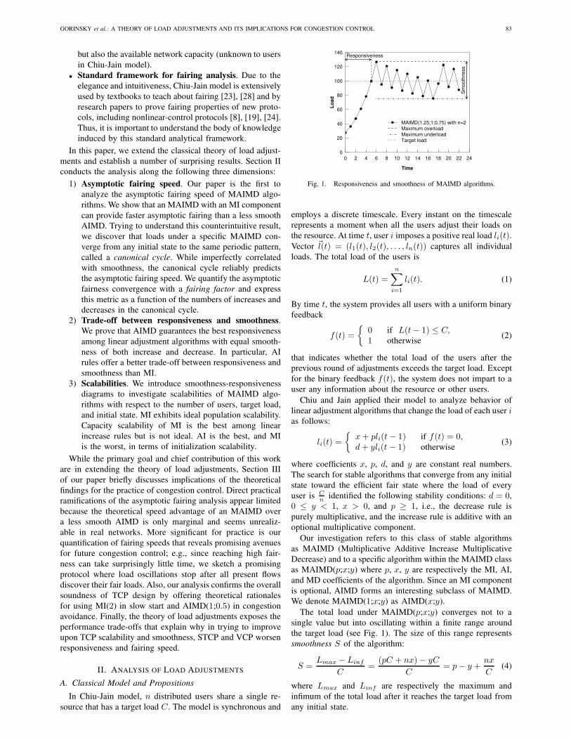
Fig. 1. Responsiveness and smoothness of MAIMD algorithms.

employs a discrete timescale. Every instant on the timescale

represents a moment when all the users adjust their loads on

the resource. At time t, user i imposes a positive real load li(t).Vector ~l(t) = (l1(t), l2(t), . . . , ln(t)) captures all individualloads. The total load of the users is

L(t) =

n∑

i=1

li(t). (1)

By time t, the system provides all users with a uniform binaryfeedback

f(t) =

{

0 if L(t − 1) ≤ C,1 otherwise

(2)

that indicates whether the total load of the users after the

previous round of adjustments exceeds the target load. Except

for the binary feedback f(t), the system does not impart to auser any information about the resource or other users.

Chiu and Jain applied their model to analyze behavior of

linear adjustment algorithms that change the load of each user ias follows:

li(t) =

{

x + pli(t − 1) if f(t) = 0,d + yli(t − 1) otherwise

(3)

where coefficients x, p, d, and y are constant real numbers.The search for stable algorithms that converge from any initial

state toward the efficient fair state where the load of every

user is Cnidentified the following stability conditions: d = 0,

0 ≤ y < 1, x > 0, and p ≥ 1, i.e., the decrease rule ispurely multiplicative, and the increase rule is additive with an

optional multiplicative component.

Our investigation refers to this class of stable algorithms

as MAIMD (Multiplicative Additive Increase Multiplicative

Decrease) and to a specific algorithm within the MAIMD class

as MAIMD(p;x;y) where p, x, y are respectively the MI, AI,and MD coefficients of the algorithm. Since an MI component

is optional, AIMD forms an interesting subclass of MAIMD.

We denote MAIMD(1;x;y) as AIMD(x;y).

The total load under MAIMD(p;x;y) converges not to asingle value but into oscillating within a finite range around

the target load (see Fig. 1). The size of this range represents

smoothness S of the algorithm:

S =Lmax − Linf

C=

(pC + nx) − yC

C= p − y +

nx

C(4)

where Lmax and Linf are respectively the maximum and

infimum of the total load after it reaches the target load from

any initial state.


Responsiveness R of the MAIMD(p;x;y) algorithm is theamount of time taken by the total load to reach the target load

from the initial state [10]:

R =

⌈

logp

(

(p−1)C+nx

(p−1)L(0)+nx

)⌉

if L(0) ≤ C, p > 1,⌈

C−L(0)nx

⌉

if L(0) ≤ C, p = 1,⌈

logy

(

CL(0)

)⌉

if L(0) > C.

(5)

Individual loads oscillate similarly to the total load but

converge infinitesimally close to each other. Fairness F (t) attime t quantifies this process of asymptotic fairing:

F (t) =

n

mini=1

li(t)

nmaxi=1

li(t). (6)

Fairness takes its values from range [0, 1] and converges to 1.An ideal algorithm would minimize both S and R as wellas maximize the fairing speed. However, a fundamental trade-

off exists between smoothness and responsiveness: values of

coefficients p, x, or y that improve responsiveness worsensmoothness. It is impossible to narrow down the MAIMD

class to a specific algorithm with optimal responsiveness and

smoothness.

With respect to the speed of fairing, Chiu and Jain observed

that whereas a single decrease does not affect fairness, a single

increase under MAIMD(p;x;y) improves fairness the mostwhen p is reduced to 1. The observation led to a propositionthat the AIMD subclass of MAIMD offers optimal fairing.

B. Asymptotic Fairing Speed

The classical assertion of the fastest fairing under AIMD is

important because it serves as the only theoretical justification

for favoring AIMD over MAIMD in TCP and other prominent

protocols. Gorinsky and Vin cast doubt on optimality of fairing

under AIMD by showing that MAIMD(p;x;y) with p > 1can raise fairness significantly higher than AIMD(x;y) afterthe same number of multiple adjustments [15]. However, this

observation neglects two aspects of the fairing problem. First,

the slower fairing after a fixed number of steps does not mean

that AIMD(x;y) fails to overcome the lag eventually and thenprovide consistently better fairness than MAIMD(p;x;y). Sec-ond, AIMD(x;y) is smoother than MAIMD(p;x;y). Since thereis the fundamental trade-off between smoothness and respon-

siveness, a similar trade-off might exist between smoothness

and fairing speed. Then, the lag of AIMD(x;y) might be dueto its smoother parameter settings, rather than the absence of

an MI component.

Hence, we start our analysis by comparing asymptotic

fairing of MAIMD and AIMD when the compared algorithms

have equal smoothness. To reason about speeds of asymptotic

fairing, we define the following notion:

Definition 1: Algorithm X provides faster asymptotic fair-ing from initial state ~l(0) than algorithm Y if

∃ τ ∀ t > τ FX(t) > FY (t) (7)

where FX(t) and FY (t) represent fairness provided at time tby algorithms X and Y respectively.As fairness asymptoticly approaches 1, the traditional rep-resentation of fairness becomes inconvenient due to accumula-

tion of nines after the decimal point. To facilitate comparison

of fairness levels during asymptotic fairing, we define a new

Time

Lo

ad

0

2

4

6

8

10

12

14

16

18

0 2 4 6 8 10 12 14 16 18 20

AIMD(1;0.5)

MAIMD(z+0.5;1;z)

Target load

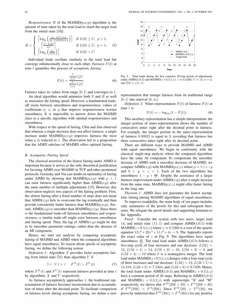
Fig. 2. Total loads during the first common 20-step period of adjustmentsunder AIMD(1;0.5) and MAIMD(z+0.5;1;z): z ≈ 0.5266, C = 14, n = 2,and ~l(0) = (11, 1).

representation that remaps fairness from its traditional range

[0, 1] into interval [0,∞]:Definition 2: Nines-representation N(t) of fairness F (t) attime t is

N(t) = − log10 (1 − F (t)). (8)

This auxiliary representation has a simple interpretation: the

integer portion of nines-representation shows the number of

consecutive nines right after the decimal point in fairness.

For example, the integer portion in the nines-representation

of fairness 0.99925 is equal to 3, revealing that fairness hasthree consecutive nines right after its decimal point.

There are different ways to provide MAIMD and AIMD

with equal smoothness. We begin in conformity with the

classical single-step analysis where the compared algorithms

have the same AI component. To compensate the smoother

increase of AIMD with a smoother decrease of MAIMD, we

compare AIMD(x;y) with MAIMD(p;x;z) where p = 1+z−yand 0 < y < z < 1. Each of the two algorithms hassmoothness 1 − y + nx

C. Despite the assurance of a larger

fairness improvement under AIMD(x;y) after a single increasefrom the same state, MAIMD(p;x;z) might offer faster fairingin the long run:

Theorem 1: AIMD does not guarantee the fastest asymp-

totic fairing among MAIMD algorithms of equal smoothness.

To improve readability, the main body of our paper includes

only summaries of the proofs for this and subsequent theo-

rems. We relegate the proof details and supporting lemmata to

the Appendix.

Proof: Consider the system with two users, target load

14, and initial state (11, 1) and compare AIMD(1;0.5) withMAIMD(z+0.5;1;z) where z ≈ 0.5266 is a root of the quarticequation 12z4 +20z3 +11z2 +4z = 9. The Appendix reportsthe exact value of z in Fig. 9. The algorithms have equalsmoothness 9

14 . The total load under AIMD(1;0.5) follows afive-step cycle of four increases and one decrease: L(5k) =12, L(5k + 1) = 14, L(5k + 2) = 16, L(5k + 3) = 8, andL(5k + 4) = 10 where k is a nonnegative integer. The totalload under MAIMD(z+0.5;1;z) changes with a four-step cycleof three increases and one decrease: L(4k) = 12, L(4k+1) ≈14.319, L(4k+2) ≈ 7.5404, and L(4k+3) ≈ 9.7409. Hence,the total loads under AIMD(1;0.5) and MAIMD(z + 0.5;1;z)have a common period of 20 steps. Referring to AIMD(1;0.5)and MAIMD(z + 0.5;1;z) with superscripts “A” and “M”respectively, we derive that FM (20k + 20) > FA(20k + 20)if FM (20k) > FA(20k). Since FM (20) > FA(20), weprove by induction that FM (20n) > FA(20n) for any positive


Time

Fa

irn

es

s

0

0.1

0.2

0.3

0.4

0.5

0.6

0.7

0.8

0.9

1

0 2 4 6 8 10 12 14 16 18 20

AIMD(1;0.5)

MAIMD(z+0.5;1;z)

Nin

es

−re

pre

se

nta

tio

n o

f fa

irn

es

s

0

1

2

3

4

5

6

7

8

9

10

11

12

0 40 80 120 160 200

Time

AIMD(1;0.5)

MAIMD(z+0.5;1;z)

180 185 190 195 20010.6

10.8

11.0

11.2

11.4

11.6

11.8

12.0

Nin

es

−re

pre

se

nta

tio

n o

f fa

irn

es

s

Time

AIMD(1;0.5)

MAIMD(z+0.5;1;z)

(a) (b) (c)

Fig. 3. Faster fairing of MAIMD(z + 0.5;1;z) over AIMD(1;0.5) when z ≈ 0.5266, C = 14, n = 2, and ~l(0) = (11, 1): (a) slight lead after the first 20steps, (b) first ten common periods of adjustments, (c) stable lead during the tenth common period.

integer n. Then, by Definition 1, AIMD does not guaranteethe fastest asymptotic fairing among MAIMD with equal

smoothness.

To illustrate the above proof, Fig. 2 shows the first com-

mon 20-step period of the total loads under the compared

algorithms. Fig. 3a shows that MAIMD(z + 0.5;1;z) acquiresa slight fairness advantage over AIMD(1;0.5) after the firstcommon period. Although the algorithms take turns in pro-

viding better fairness early on, MAIMD(z+0.5;1;z) overtakesAIMD(1;0.5) for good at time 67 and then unfailingly yieldshigher fairness, as Fig. 3b indicates. Fig. 3c shows the per-

sistent lag of fairness under the AIMD algorithm during the

tenth common period of the total loads.

To understand reasons for the counterintuitive Theo-

rem 1, we examine sensitivities of the fairing speed under

AIMD(1;0.5) and MAIMD(z + 0.5;1;z) to the system con-figuration. Fig. 4a shows that MAIMD(z + 0.5;1;z) outpacesAIMD(1;0.5) after 200 steps from all examined initial loads.Hence, MAIMD(z +0.5;1;z) excels not because of starting ina special state that forces the total loads under the algorithms

to oscillate with the common period disadvantageous for

AIMD(1;0.5). Fig. 4b hints at a likely reason for the resilienceto the choice if the initial load: from different initial states,

the total load under MAIMD converges to the same periodic

pattern of oscillations. We represent this periodic pattern with

a canonical cycle:

Definition 3: A canonical cycle of an adjustment algorithm

is the shortest finite repeating sequence of total loads under

the algorithm, starting at the smallest value.

For example, the canonical cycle of AIMD(1;0.5) in theabove system with C = 14 and n = 2 is (8,10,12,14,16).Convergence to a canonical cycle is a property of all MAIMD

algorithms:

Theorem 2: The total load under an MAIMD algorithm

converges to a unique canonical cycle.

Proof: Consider a system with target load C, n users,and MAIMD(p;x;z) control. Case 1: If pzC + nx > C,then exactly one increase follows each decrease sequence,

and lengths of all decrease sequences that follow an increase

differ by at most one step. Let m denote⌈

logzC

pzC+nx

⌉

. If

m ≥ logzC

pC+nx, then the total load converges to the periodic

pattern of one increase and m decreases. If m < logzC

pC+nx,

then each decrease sequence contains either m or m + 1steps, depending on whether the underload after the previous

decrease sequence is at most z−mC−nxp

or above. In this range

of m, load oscillations also converge from any initial state toa unique periodic pattern. Case 2 (which covers all settings

that Case 1 does not): If z(pC + nx) ≤ C, then exactly onedecrease follows each increase sequence, and the proof mirrors

the reasoning in Case 1.

As per the above, load oscillations converge from any initial

state to the same periodic pattern. With T denoting the periodduration, we express the total load at time t = τ + kT as

L(t) = qkL(τ) +1 − qk

1 − qr (9)

where τ represents an initial transient (which depends on theinitial state), k is the number of subsequent periods, and valuesof q and r depend on the phase within the period but not onthe initial load. Since qk → 0 and L(t) → r

1−qwhen t → ∞,

the total load converges from any initial state to values r1−q

that form a unique canonical cycle.

Theorem 2 suggests that the asymptotic fairing speed of

an MAIMD is determined by the canonical cycle, rather than

smoothness. This leads us to the insight that MAIMD(p;x;y)with p > 1 might converge to fairness faster than an AIMDwith worse smoothness in terms of both increase and decrease:

Theorem 3: An MAIMD algorithm with an MI component

can provide faster asymptotic fairing than an AIMD algorithm

with worse smoothness of both increase and decrease.

Proof: For the same system configuration as in the proof

of Theorem 1, we compare the asymptotic fairing speeds

of AIMD(1;0.5) and MAIMD(1.00014;0.999;y) where y =14001−(100.0143

−106)· 99970

1.000143·14001 ≈ 0.5716. The two proofs are similar

in general but this proof overcomes a new subtle challenge

that arises because MAIMD(1.00014;0.999;y) converges to thevalues of its canonical cycle asymptotically instead of adhering

to them exactly.

The presence of the MI component in the MAIMD is not

essential for the above proof. For instance, AIMD(x;y) withx = 0.9999 and y = 13336

23335 ≈ 0.5715 also provides fasterasymptotic fairing than AIMD(1;0.5) despite being smootherin terms of both increase and decrease.

Corollary 1: There exists no fundamental trade-off between

the asymptotic fairing speed and smoothness.

Unlike the initial state, the target load does affect the

qualitative outcome of comparing the fairing speeds of the

algorithms from the proof of Theorem 1. Fig. 4c shows that

MAIMD(z+0.5;1;z) supplies faster fairing than AIMD(1;0.5)only in a narrow region around the target load 14. Furthermore,raising the target load slightly beyond this region makes the


Nin

es

−re

pre

se

nta

tio

n o

f fa

irn

es

s a

t ti

me

20

0

11.75

11.8

11.85

11.9

11.95

12

12.05

7 8 9 10 11 12 13 14 15

Initial load of the first user

AIMD(1;0.5)MAIMD(z+0.5;1;z)

Time

Lo

ad

0

2

4

6

8

10

12

14

16

18

0 3 6 9 12 15 18 21 24 27 30

MAIMD(z+0.5;1;z) with initial state (10.6;1)MAIMD(z+0.5;1;z) with initial state (10.7;1)Target load

Target load

Nin

es

−re

pre

se

nta

tio

n o

f fa

irn

es

s a

t ti

me

20

0

8

9

10

11

12

13

14

15

10 12 14 16 18 20 22

AIMD(1;0.5)MAIMD(z+0.5;1;z)

(a) (b) (c)

Fig. 4. Sensitivities of the fairing speed under AIMD(1;0.5) and MAIMD(z + 0.5;1;z) to the system configuration, z ≈ 0.5266, n = 2, and l2(0) = 1:(a) dependence on the initial state when C = 14; (b) convergence to the canonical cycle; (c) sensitivity to the target load when l1(0) = 11.

1.0 1.1 1.2 1.3 1.4

4

6

8

10

12

14

Multiplicative increase coefficient p of MAIMD(p;1;z)

Nin

es

−re

pre

se

nta

tio

n o

f fa

irn

es

s a

t ti

me

20

0

Target load 14

Target load 17.1

Target load 20.2

0.6 0.7 0.8 0.9 1.0 1.1 1.2

4

6

8

10

12

14

Additive increase coefficient x of MAIMD(z+0.5;x;z)

Nin

es

−re

pre

se

nta

tio

n o

f fa

irn

es

s a

t ti

me

20

0

Target load 14

Target load 17.1

Target load 20.2

0.3 0.4 0.5 0.6 0.7

6

8

10

12

14

16

Multiplicative decrease coefficient y of MAIMD(z+0.5;1;y)

Nin

es

−re

pre

se

nta

tio

n o

f fa

irn

es

s a

t ti

me

20

0

Target load 14

Target load 17.1

Target load 20.2

Fig. 5. Sensitivities of the fairing speed to MAIMD coefficients: z ≈ 0.5266, n = 2, and ~l(0) = (11, 1).

canonical cycle of MAIMD(z+0.5;1;z) change frequently. Thecanonical cycle of AIMD(1;0.5) exhibits similar sensitivitiesto the target load. For instance, when the target load reduces

from 14 to 13.99, the canonical cycle of AIMD(1;0.5) changesfrom (8,10,12,14,16) to a 39-entry sequence that starts atits minimum value 6.996, peaks 8 times, and contains themaximum value 15.984 in the 35-th entry.We now study sensitivities of the fairing speed to MAIMD

coefficients. Fig. 5 agrees with Corollary 1 that no funda-

mental trade-off exists between smoothness and asymptotic

fairing speed. The graphs also show definite, though non-

monotonic, dependencies of the fairing speed on the MAIMD

coefficients that determine smoothness. In general, the fairing

speed improves as the MI or MD coefficient decreases, or the

AI coefficient increases.

Fig. 3b indicates that after an initial transient, average

improvement of fairness in its nines-representation occurs at a

stable rate. Hence, to characterize the asymptotic fairing speed

of MAIMD algorithms, we introduce the following metric

called a fairing factor:

Definition 4: Fairing factor G of an MAIMD algorithm is

G = limt→∞

N(t) − N(0)

t. (10)

Then, we express the fairing factor of an MAIMD in terms

of properties of the canonical cycle:

Theorem 4: The fairing factor of MAIMD(p;x;z) equals

G = −I log10 p + D log10 z

I + D(11)

where I and D are respectively the number of increases anddecreases in the canonical cycle of the algorithm.

Proof: Denoting the maximum individual load at time t aslmax(t), we express improvement of fairness after one increaseas

N(t) − N(t − 1) = log10

lmax(t)

lmax(t − 1)− log10 p (12)

and lack of change in fairness after one decrease as

N(t) − N(t − 1) = log10

lmax(t)

lmax(t − 1)− log10 z. (13)

Then, average improvement of fairness from time 0 to t is

N(t) − N(0)

t=

log10lmax(t)lmax(0) − i(t) log10 p − d(t) log10 z

t

where i(t) and d(t) are respectively the overall number ofincreases and decreases from time 0 to t. Since load oscilla-tions converge to the canonical cycle, we apply Definition 4

to derive Equation 11.

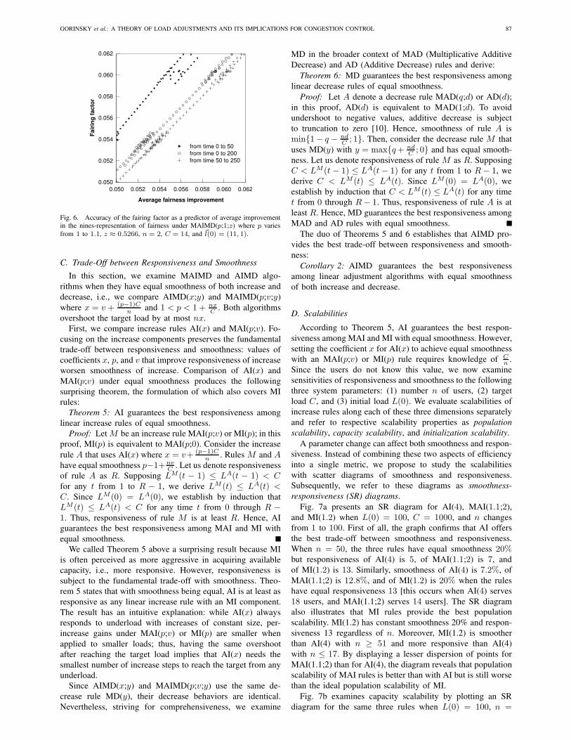
It is interesting that the AI coefficient x affects the fairingfactor of MAIMD(p;x;z) only indirectly through the numbersof increases and decreases in the canonical cycle. Fig. 6

illustrates the accuracy of the fairing factor as a predictor

of average fairness improvement under MAIMD(p;1;z) wherez ≈ 0.5266 and p varies from 1 to 1.1. For time interval[0,50], the prediction is significantly off due to the initial tran-sient. Extension of the averaging interval to [0,200] subduesthe contribution from the initial transient and improves the

prediction dramatically. Finally, shifting the averaging interval

to [50,250] yields an almost perfect prediction, indicating thatthe fairing factor is an appropriate metric for representing the

asymptotic fairing speed of an MAIMD algorithm.


0.050 0.052 0.054 0.056 0.058 0.060 0.062

0.050

0.052

0.054

0.056

0.058

0.060

0.062

Average fairness improvement

Fa

irin

g f

ac

tor

from time 0 to 50

from time 0 to 200

from time 50 to 250

Fig. 6. Accuracy of the fairing factor as a predictor of average improvementin the nines-representation of fairness under MAIMD(p;1;z) where p varies

from 1 to 1.1, z ≈ 0.5266, n = 2, C = 14, and ~l(0) = (11, 1).

C. Trade-Off between Responsiveness and Smoothness

In this section, we examine MAIMD and AIMD algo-

rithms when they have equal smoothness of both increase and

decrease, i.e., we compare AIMD(x;y) and MAIMD(p;v;y)where x = v + (p−1)C

nand 1 < p < 1 + nx

C. Both algorithms

overshoot the target load by at most nx.First, we compare increase rules AI(x) and MAI(p;v). Fo-cusing on the increase components preserves the fundamental

trade-off between responsiveness and smoothness: values of

coefficients x, p, and v that improve responsiveness of increaseworsen smoothness of increase. Comparison of AI(x) andMAI(p;v) under equal smoothness produces the followingsurprising theorem, the formulation of which also covers MI

rules:

Theorem 5: AI guarantees the best responsiveness among

linear increase rules of equal smoothness.

Proof: LetM be an increase rule MAI(p;v) or MI(p); in thisproof, MI(p) is equivalent to MAI(p;0). Consider the increaserule A that uses AI(x) where x = v+ (p−1)C

n. RulesM and A

have equal smoothness p−1+nvC. Let us denote responsiveness

of rule A as R. Supposing LM (t − 1) ≤ LA(t − 1) < Cfor any t from 1 to R − 1, we derive LM (t) ≤ LA(t) <C. Since LM (0) = LA(0), we establish by induction thatLM (t) ≤ LA(t) < C for any time t from 0 through R −1. Thus, responsiveness of rule M is at least R. Hence, AIguarantees the best responsiveness among MAI and MI with

equal smoothness.

We called Theorem 5 above a surprising result because MI

is often perceived as more aggressive in acquiring available

capacity, i.e., more responsive. However, responsiveness is

subject to the fundamental trade-off with smoothness. Theo-

rem 5 states that with smoothness being equal, AI is at least as

responsive as any linear increase rule with an MI component.

The result has an intuitive explanation: while AI(x) alwaysresponds to underload with increases of constant size, per-

increase gains under MAI(p;v) or MI(p) are smaller whenapplied to smaller loads; thus, having the same overshoot

after reaching the target load implies that AI(x) needs thesmallest number of increase steps to reach the target from any

underload.

Since AIMD(x;y) and MAIMD(p;v;y) use the same de-crease rule MD(y), their decrease behaviors are identical.Nevertheless, striving for comprehensiveness, we examine

MD in the broader context of MAD (Multiplicative Additive

Decrease) and AD (Additive Decrease) rules and derive:

Theorem 6: MD guarantees the best responsiveness among

linear decrease rules of equal smoothness.

Proof: Let A denote a decrease rule MAD(q;d) or AD(d);in this proof, AD(d) is equivalent to MAD(1;d). To avoidundershoot to negative values, additive decrease is subject

to truncation to zero [10]. Hence, smoothness of rule A ismin{1− q − nd

C; 1}. Then, consider the decrease rule M that

uses MD(y) with y = max{q + ndC

; 0} and has equal smooth-ness. Let us denote responsiveness of ruleM as R. SupposingC < LM (t − 1) ≤ LA(t − 1) for any t from 1 to R − 1, wederive C < LM (t) ≤ LA(t). Since LM (0) = LA(0), weestablish by induction that C < LM (t) ≤ LA(t) for any timet from 0 through R − 1. Thus, responsiveness of rule A is atleast R. Hence, MD guarantees the best responsiveness amongMAD and AD rules with equal smoothness.

The duo of Theorems 5 and 6 establishes that AIMD pro-

vides the best trade-off between responsiveness and smooth-

ness:

Corollary 2: AIMD guarantees the best responsiveness

among linear adjustment algorithms with equal smoothness

of both increase and decrease.

D. Scalabilities

According to Theorem 5, AI guarantees the best respon-

siveness among MAI and MI with equal smoothness. However,

setting the coefficient x for AI(x) to achieve equal smoothnesswith an MAI(p;v) or MI(p) rule requires knowledge of C

n.

Since the users do not know this value, we now examine

sensitivities of responsiveness and smoothness to the following

three system parameters: (1) number n of users, (2) targetload C, and (3) initial load L(0). We evaluate scalabilities ofincrease rules along each of these three dimensions separately

and refer to respective scalability properties as population

scalability, capacity scalability, and initialization scalability.

A parameter change can affect both smoothness and respon-

siveness. Instead of combining these two aspects of efficiency

into a single metric, we propose to study the scalabilities

with scatter diagrams of smoothness and responsiveness.

Subsequently, we refer to these diagrams as smoothness-

responsiveness (SR) diagrams.

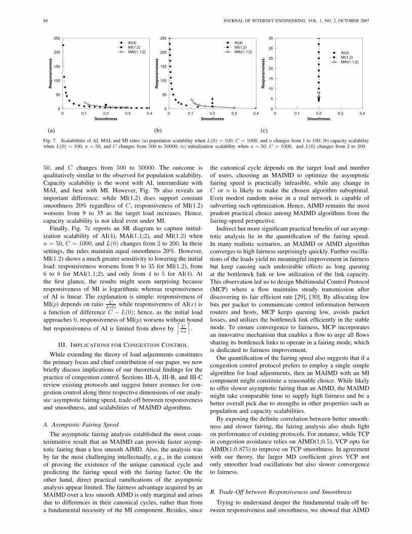
Fig. 7a presents an SR diagram for AI(4), MAI(1.1;2),and MI(1.2) when L(0) = 100, C = 1000, and n changesfrom 1 to 100. First of all, the graph confirms that AI offersthe best trade-off between smoothness and responsiveness.

When n = 50, the three rules have equal smoothness 20%but responsiveness of AI(4) is 5, of MAI(1.1;2) is 7, andof MI(1.2) is 13. Similarly, smoothness of AI(4) is 7.2%, ofMAI(1.1;2) is 12.8%, and of MI(1.2) is 20% when the ruleshave equal responsiveness 13 [this occurs when AI(4) serves18 users, and MAI(1.1;2) serves 14 users]. The SR diagramalso illustrates that MI rules provide the best population

scalability. MI(1.2) has constant smoothness 20% and respon-

siveness 13 regardless of n. Moreover, MI(1.2) is smootherthan AI(4) with n ≥ 51 and more responsive than AI(4)with n ≤ 17. By displaying a lesser dispersion of points forMAI(1.1;2) than for AI(4), the diagram reveals that population

scalability of MAI rules is better than with AI but is still worse

than the ideal population scalability of MI.

Fig. 7b examines capacity scalability by plotting an SR

diagram for the same three rules when L(0) = 100, n =


Re

sp

on

siv

en

es

s

0

50

100

150

200

250

0 0.1 0.2 0.3 0.4

Smoothness

AI(4)

MI(1.2)

MAI(1.1;2)

Re

sp

on

siv

en

es

s

0

50

100

150

200

250

0 0.1 0.2 0.3 0.4

Smoothness

AI(4)

MI(1.2)

MAI(1.1;2)

Re

sp

on

siv

en

es

s

0

5

10

15

20

25

30

35

0 0.1 0.2 0.3 0.4

Smoothness

AI(4)

MI(1.2)

MAI(1.1;2)

(a) (b) (c)

Fig. 7. Scalabilities of AI, MAI, and MI rules: (a) population scalability when L(0) = 100, C = 1000, and n changes from 1 to 100; (b) capacity scalabilitywhen L(0) = 100, n = 50, and C changes from 500 to 50000; (c) initialization scalability when n = 50, C = 1000, and L(0) changes from 2 to 200.

50, and C changes from 500 to 50000. The outcome isqualitatively similar to the observed for population scalability.

Capacity scalability is the worst with AI, intermediate with

MAI, and best with MI. However, Fig. 7b also reveals an

important difference: while MI(1.2) does support constant

smoothness 20% regardless of C, responsiveness of MI(1.2)worsens from 9 to 35 as the target load increases. Hence,

capacity scalability is not ideal even under MI.

Finally, Fig. 7c reports an SR diagram to capture initial-

ization scalability of AI(4), MAI(1.1;2), and MI(1.2) whenn = 50, C = 1000, and L(0) changes from 2 to 200. In thesesettings, the rules maintain equal smoothness 20%. However,

MI(1.2) shows a much greater sensitivity to lowering the initialload: responsiveness worsens from 9 to 35 for MI(1.2), from6 to 8 for MAI(1.1;2), and only from 4 to 5 for AI(4). Atthe first glance, the results might seem surprising because

responsiveness of MI is logarithmic whereas responsiveness

of AI is linear. The explanation is simple: responsiveness of

MI(p) depends on ratio CL(0) while responsiveness of AI(x) is

a function of difference C − L(0); hence, as the initial loadapproaches 0, responsiveness of MI(p) worsens without bound

but responsiveness of AI is limited from above by⌈

Cnx

⌉

.

III. IMPLICATIONS FOR CONGESTION CONTROL

While extending the theory of load adjustments constitutes

the primary focus and chief contribution of our paper, we now

briefly discuss implications of our theoretical findings for the

practice of congestion control. Sections III-A, III-B, and III-C

review existing protocols and suggest future avenues for con-

gestion control along three respective dimensions of our analy-

sis: asymptotic fairing speed, trade-off between responsiveness

and smoothness, and scalabilities of MAIMD algorithms.

A. Asymptotic Fairing Speed

The asymptotic fairing analysis established the most coun-

terintuitive result that an MAIMD can provide faster asymp-

totic fairing than a less smooth AIMD. Also, the analysis was

by far the most challenging intellectually, e.g., in the context

of proving the existence of the unique canonical cycle and

predicting the fairing speed with the fairing factor. On the

other hand, direct practical ramifications of the asymptotic

analysis appear limited. The fairness advantage acquired by an

MAIMD over a less smooth AIMD is only marginal and arises

due to differences in their canonical cycles, rather than from

a fundamental necessity of the MI component. Besides, since

the canonical cycle depends on the target load and number

of users, choosing an MAIMD to optimize the asymptotic

fairing speed is practically infeasible, while any change in

C or n is likely to make the chosen algorithm suboptimal.Even modest random noise in a real network is capable of

subverting such optimization. Hence, AIMD remains the most

prudent practical choice among MAIMD algorithms from the

fairing-speed perspective.

Indirect but more significant practical benefits of our asymp-

totic analysis lie in the quantification of the fairing speed.

In many realistic scenarios, an MAIMD or AIMD algorithm

converges to high fairness surprisingly quickly. Further oscilla-

tions of the loads yield no meaningful improvement in fairness

but keep causing such undesirable effects as long queuing

at the bottleneck link or low utilization of the link capacity.

This observation led us to design Multimodal Control Protocol

(MCP) where a flow maintains steady transmission after

discovering its fair efficient rate [29], [30]. By allocating few

bits per packet to communicate control information between

routers and hosts, MCP keeps queuing low, avoids packet

losses, and utilizes the bottleneck link efficiently in the stable

mode. To ensure convergence to fairness, MCP incorporates

an innovative mechanism that enables a flow to urge all flows

sharing its bottleneck links to operate in a fairing mode, which

is dedicated to fairness improvement.

Our quantification of the fairing speed also suggests that if a

congestion control protocol prefers to employ a single simple

algorithm for load adjustments, then an MAIMD with an MI

component might constitute a reasonable choice. While likely

to offer slower asymptotic fairing than an AIMD, the MAIMD

might take comparable time to supply high fairness and be a

better overall pick due to strengths in other properties such as

population and capacity scalabilities.

By exposing the definite correlation between better smooth-

ness and slower fairing, the fairing analysis also sheds light

on performance of existing protocols. For instance, while TCP

in congestion avoidance relies on AIMD(1;0.5), VCP opts forAIMD(1;0.875) to improve on TCP smoothness. In agreementwith our theory, the larger MD coefficient gives VCP not

only smoother load oscillations but also slower convergence

to fairness.

B. Trade-Off between Responsiveness and Smoothness

Trying to understand deeper the fundamental trade-off be-

tween responsiveness and smoothness, we showed that AIMD


Congestion window (cwnd) upon loss

Ro

un

d−

trip

tim

es t

o r

esto

re c

wn

d

0

1

2

3

4

5

6

7

8

9

10

11

12

13

14

15

20 30 40 50 60 70 80 90 100

STCP

STCP with AI(1) when cwnd

is between 16 and 100

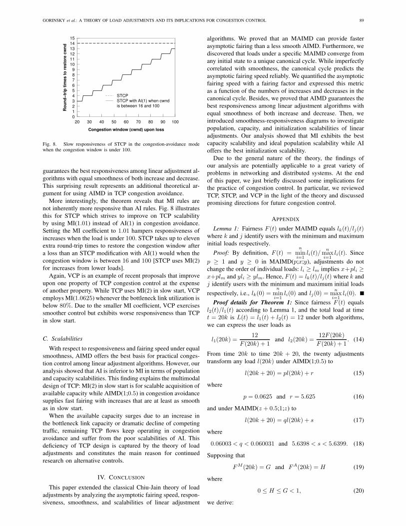
Fig. 8. Slow responsiveness of STCP in the congestion-avoidance modewhen the congestion window is under 100.

guarantees the best responsiveness among linear adjustment al-

gorithms with equal smoothness of both increase and decrease.

This surprising result represents an additional theoretical ar-

gument for using AIMD in TCP congestion avoidance.

More interestingly, the theorem reveals that MI rules are

not inherently more responsive than AI rules. Fig. 8 illustrates

this for STCP which strives to improve on TCP scalability

by using MI(1.01) instead of AI(1) in congestion avoidance.Setting the MI coefficient to 1.01 hampers responsiveness ofincreases when the load is under 100. STCP takes up to elevenextra round-trip times to restore the congestion window after

a loss than an STCP modification with AI(1) would when thecongestion window is between 16 and 100 [STCP uses MI(2)for increases from lower loads].

Again, VCP is an example of recent proposals that improve

upon one property of TCP congestion control at the expense

of another property. While TCP uses MI(2) in slow start, VCPemploys MI(1.0625) whenever the bottleneck link utilization isbelow 80%. Due to the smaller MI coefficient, VCP exercisessmoother control but exhibits worse responsiveness than TCP

in slow start.

C. Scalabilities

With respect to responsiveness and fairing speed under equal

smoothness, AIMD offers the best basis for practical conges-

tion control among linear adjustment algorithms. However, our

analysis showed that AI is inferior to MI in terms of population

and capacity scalabilities. This finding explains the multimodal

design of TCP: MI(2) in slow start is for scalable acquisition ofavailable capacity while AIMD(1;0.5) in congestion avoidancesupplies fast fairing with increases that are at least as smooth

as in slow start.

When the available capacity surges due to an increase in

the bottleneck link capacity or dramatic decline of competing

traffic, remaining TCP flows keep operating in congestion

avoidance and suffer from the poor scalabilities of AI. This

deficiency of TCP design is captured by the theory of load

adjustments and constitutes the main reason for continued

research on alternative controls.

IV. CONCLUSION

This paper extended the classical Chiu-Jain theory of load

adjustments by analyzing the asymptotic fairing speed, respon-

siveness, smoothness, and scalabilities of linear adjustment

algorithms. We proved that an MAIMD can provide faster

asymptotic fairing than a less smooth AIMD. Furthermore, we

discovered that loads under a specific MAIMD converge from

any initial state to a unique canonical cycle. While imperfectly

correlated with smoothness, the canonical cycle predicts the

asymptotic fairing speed reliably. We quantified the asymptotic

fairing speed with a fairing factor and expressed this metric

as a function of the numbers of increases and decreases in the

canonical cycle. Besides, we proved that AIMD guarantees the

best responsiveness among linear adjustment algorithms with

equal smoothness of both increase and decrease. Then, we

introduced smoothness-responsiveness diagrams to investigate

population, capacity, and initialization scalabilities of linear

adjustments. Our analysis showed that MI exhibits the best

capacity scalability and ideal population scalability while AI

offers the best initialization scalability.

Due to the general nature of the theory, the findings of

our analysis are potentially applicable to a great variety of

problems in networking and distributed systems. At the end

of this paper, we just briefly discussed some implications for

the practice of congestion control. In particular, we reviewed

TCP, STCP, and VCP in the light of the theory and discussed

promising directions for future congestion control.

APPENDIX

Lemma 1: Fairness F (t) under MAIMD equals lk(t)/lj(t)where k and j identify users with the minimum and maximuminitial loads respectively.

Proof: By definition, F (t) =n

mini=1

li(t)/n

maxi=1

li(t). Since

p ≥ 1 and y ≥ 0 in MAIMD(p;x;y), adjustments do notchange the order of individual loads: li ≥ lm implies x+pli ≥x+plm and yli ≥ ylm. Hence, F (t) = lk(t)/lj(t) where k andj identify users with the minimum and maximum initial loads

respectively, i.e., lk(0) =n

mini=1

li(0) and lj(0) =n

maxi=1

li(0).

Proof details for Theorem 1: Since fairness F (t) equalsl2(t)/l1(t) according to Lemma 1, and the total load at timet = 20k is L(t) = l1(t) + l2(t) = 12 under both algorithms,we can express the user loads as

l1(20k) =12

F (20k) + 1and l2(20k) =

12F (20k)

F (20k) + 1. (14)

From time 20k to time 20k + 20, the twenty adjustmentstransform any load l(20k) under AIMD(1;0.5) to

l(20k + 20) = pl(20k) + r (15)

where

p = 0.0625 and r = 5.625 (16)

and under MAIMD(z + 0.5;1;z) to

l(20k + 20) = ql(20k) + s (17)

where

0.06003 < q < 0.060031 and 5.6398 < s < 5.6399. (18)

Supposing that

FM (20k) = G and FA(20k) = H (19)

where

0 ≤ H ≤ G < 1, (20)

we derive:


z =1

2

0

B

B

B

@

v

u

u

u

u

t

1

6+

1415

363p

24√

4978461 − 5869

−

3p

24√

4978461 − 5869

36+

8

27

r

1

12−

1415

363√

24√

4978461−5869

+3√

24√

4978461−5869

36

−

v

u

u

t

1

12−

1415

363p

24√

4978461 − 5869

+

3p

24√

4978461 − 5869

36−

5

6

1

A

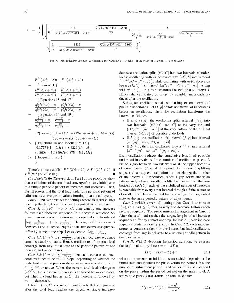
Fig. 9. Multiplicative decrease coefficient z for MAIMD(z + 0.5;1;z) in the proof of Theorem 1 (z ≈ 0.5266).

FM (20k + 20) − FA(20k + 20)

= { Lemma 1 }

lM2 (20k + 20)

lM1 (20k + 20)−

lA2 (20k + 20)

lA1 (20k + 20)

= { Equations 15 and 17 }

qlM2 (20k) + s

qlM1 (20k) + s−

plA2 (20k) + r

plA1 (20k) + r


q 12GG+1 + s

q 12G+1 + s

−p 12H

H+1 + r

p 12H+1 + r

=12

(

(ps − qr)(1 − GH) + (12pq + ps + qr)(G − H))

(12q + s + sG)(12p + r + rH)

> { Equations 16 and Inequalities 18 }

0.17775(1− GH) + 8.8221(G− H)

(6.3603 + 5.6399G)(6.375 + 5.625H)

> { Inequalities 20 }

0.

Therefore, we establish FM (20k + 20) > FA(20k + 20) ifFM (20k) > FA(20k).Proof details for Theorem 2: In Part I of the proof, we show

that oscillations of the total load converge from any initial state

to a unique periodic pattern of increases and decreases. Then,

Part II proves that the total load under this periodic pattern of

adjustments converges to values forming a canonical cycle.

Part I: First, we consider the settings where an increase after

reaching the target load is at least as potent as a decrease.

Case 1: If pzC + nx > C, then exactly one increasefollows each decrease sequence. In a decrease sequence be-

tween two increases, the number of steps belongs to interval[

logzC

pzC+nx; 1 + logz

CpC+nx

)

. The length of this interval is

between 1 and 2. Hence, lengths of all such decrease sequences

differ by at most one step. Let m denote⌈

logzC

pzC+nx

⌉

.

Case 1.1: If m ≥ logzC

pC+nx, then each decrease sequence

contains exactly m steps. Hence, oscillations of the total loadconverge from any initial state to the periodic pattern of one

increase and m decreases.Case 1.2: If m < logz

CpC+nx

, then each decrease sequence

contains either m or m + 1 steps, depending on whether theunderload after the previous decrease sequence is at most L =z−mC−nx

por above. When the current total load belongs to

(zC; L], the subsequent increase is followed by m decreases,but when the load lies in (L; C], the increase is followed bym + 1 decreases.Interval (zC; C] consists of underloads that are possibleafter the total load reaches the target. A single increase-

decrease oscillation splits (zC; C] into two intervals of under-loads: oscillating with m decreases lifts (zC; L] into interval(

zm+1pC + zmnx; C]

, while oscillating withm+1 decreaseslowers (L; C] into interval

(

zC; zm+1pC + zm+1nx]

. A gap

with width (1 − z)zmnx separates the two created intervals.Hence, the cumulative coverage by possible underloads re-

duces after the oscillation.

Subsequent oscillations make similar impacts on intervals of

possible underloads. Let (f ; g] denote an interval of underloadsbefore an oscillation. Then, the oscillation transforms the

interval as follows:

• If L ∈ (f ; g), the oscillation splits interval (f ; g] intotwo intervals: (zm(pf + nx); C] at the very top and(

zC; zm+1(pg + nx)]

at the very bottom of the original

interval (zC; C] of possible underloads.• If L ≥ g, the oscillation lifts interval (f ; g] into interval

(zm(pf + nx); zm(pg + nx)].• If L ≤ f , then the oscillation lowers (f ; g] into interval

(

zm+1(pf + nx); zm+1(pg + nx)]

.

Each oscillation reduces the cumulative length of possible

underload intervals. A finite number of oscillations places Linside a gap between two intervals or at the upper border gof some interval (f ; g]. At this point, the process of splittingstops, and subsequent oscillations do not change the number

of the intervals. Furthermore, since a gap forms under an

interval only when an oscillation lifts the interval from the very

bottom of (zC; C], each of the stabilized number of intervalsis reachable from every other interval through a finite sequence

of oscillations. Hence, the total load converges from any initial

state to the same periodic pattern of adjustments.

Case 2 (which covers all settings that Case 1 does not):

If z(pC + nx) ≤ C, then exactly one decrease follows eachincrease sequence. The proof mirrors the argument in Case 1.

After the total load reaches the target, lengths of all increase

sequences differ by at most one step. In Case 2.1, each increase

sequence contains exactly j steps. In Case 2.2, each increasesequence contains either j or j +1 steps, but load oscillationsconverge from any initial state to a unique periodic pattern in

this case as well.

Part II: With T denoting the period duration, we expressthe total load at any time t = τ + kT as

L(t) = qL(t − T ) + r (21)

where τ represents an initial transient (which depends on theinitial state and includes the phase within the period), k is thenumber of subsequent periods, and values of q and r dependon the phase within the period but not on the initial load. A

series of k periods transforms the total load into:

L(t) = qkL(τ) +1 − qk

1 − qr. (22)


As time advances, the contribution from L(τ) into the currentload diminishes, and L(t) becomes shaped by the cumulativeimpact of intermediate additive increases, i.e., qk → 0 andL(t) → r

1−qwhen t → ∞. Hence, the total load converges

from any initial state to values r1−q

that form a unique

canonical cycle.

Proof details for Theorem 3: According to Theorem 2,

the total load under MAIMD(1.00014;0.999;y) converges to aunique canonical cycle, which is: L(4k) ≈ 10.0019, L(4k +1) ≈ 12.0013, L(4k + 2) = 14.001, and L(4k + 3) ≈ 8.0028.

From time 20k+5 to time 20k+25, the twenty adjustmentstransform any load l(20k + 5) under AIMD(1;0.5) to

l(20k + 25) = pl(20k + 5) + r (23)

where

p = 0.0625 and r = 5.625 (24)

and under MAIMD(1.00014;0.999;y) to

l(20k + 25) = ql(20k + 5) + s (25)

where

0.06114 < q < 0.061141 and 5.6337 < s < 5.6338. (26)

Since fairness F (20k + 5) is l2(20k + 5)/l1(20k + 5) ac-cording to Lemma 1, and total load L(20k + 5) equalsl1(20k + 5) + l2(20k + 5), we express the user loads at timet = 20k + 5 under each of the algorithms as:

l1(t) =L(t)

F (t) + 1and l2(t) =

L(t)F (t)

F (t) + 1. (27)

The total load under AIMD(1;0.5) is equal to

LA(20k + 5) = 12. (28)

We prove by induction for any integer k ≥ 7 that the totalload under MAIMD(1.00014;0.999;y) is bounded from aboveas:

LM (20k + 5) < 12.0014. (29)

We also observe that FM (145) > FA(145). Supposing that

FM (20k + 5) = G and FA(20k + 5) = H (30)

where

0 ≤ H ≤ G < 1, (31)

we derive:

FM (20k + 25)− FA(20k + 25)

= { Lemma 1 }

lM2 (20k + 25)

lM1 (20k + 25)−

lA2 (20k + 25)

lA1 (20k + 25)


qlM2 (20k + 5) + s

qlM1 (20k + 5) + s−

plA2 (20k + 5) + r

plA1 (20k + 5) + r

= { Equations 27, 30, and 28 }

q LM (20k+5)GG+1 + s

q LM (20k+5)G+1 + s

−p 12H

H+1 + r

p 12H+1 + r

> { Inequalities 29 and 31 }

q 12.0014GG+1 + s

q 12.0014G+1 + s

−p 12H

H+1 + r

p 12H+1 + r

> { Equations 24 and Inequalities 26 }

0.09777(1− GH) + 8.903(G− H)

(6.3676 + 5.6338G)(6.375 + 5.625H)

> { Inequalities 31 }

0.

Therefore, we establish by induction that FM (20k + 5) >FA(20k+5) for any integer k ≥ 7. MAIMD(1.00014;0.999;y)provides faster asymptotic fairing than AIMD(1;0.5).

Proof details for Theorem 4: An increase at time t improvesthe nines-representation of fairness under MAIMD(p;x;z) by:

N(t) − N(t − 1)

= { Definition 2 and Lemma 1 }

log10

(

1 −lmin(t − 1)

lmax(t − 1)

)

− log10

(

1 −lmin(t)

lmax(t)

)

=

log10

(

lmax(t − 1) − lmin(t − 1)

lmax(t − 1)·

lmax(t)

lmax(t) − lmin(t)

)

= { li(t) = x + pli(t − 1) for both i ∈ {max, min} }

log10

lmax(t)

plmax(t − 1),

i.e.,

N(t) − N(t − 1) = log10

lmax(t)

lmax(t − 1)− log10 p. (32)

A decrease at time t does not affect fairness but withderivations similar to the above, we express the lack of change

as:

N(t) − N(t − 1) = log10

lmax(t)

lmax(t − 1)− log10 z. (33)

To compute the average improvement in the nines-

representation of fairness from time 0 to t, we represent theoverall number of increases and decreases during this time

interval as i(t) and d(t) respectively and derive:


N(t) − N(0)

=t

∑

τ=1

(N(τ) − N(τ − 1))

= { Equations 32 and 33 }t

∑

τ=1

log10

lmax(τ)

lmax(τ − 1)− i(t) log10 p − d(t) log10 z

=

log10

t∏

τ=1

lmax(τ)

lmax(τ − 1)− i(t) log10 p − d(t) log10 z

=

log10

lmax(t)

lmax(0)− i(t) log10 p − d(t) log10 z.

Then, we express the fairing factor of MAIMD(p;x;z)algorithm as follows:

G

= { Definition 4 }

limt→∞

N(t) − N(0)

t= { previous derivation }

limt→∞

log10lmax(t)lmax(0) − i(t) log10 p − d(t) log10 z

t= { lmax(t) is bounded from above and below }

−

(

limt→∞

i(t)

t

)

log10 p −

(

limt→∞

d(t)

t

)

log10 z

= { load oscillations converge to the canonical cycle }

−I

I + Dlog10 p −

D

I + Dlog10 z

where I and D are respectively the number of increases anddecreases in the canonical cycle. Hence, the fairing factor is:

G = −I log10 p + D log10 z

I + D. (34)

Proof details for Theorem 5:

LM (t)

= { Increase under rule M }

pLM (t − 1) + nv

≤ { Hypothesis LM (t − 1) ≤ LA(t − 1) < C }

pLA(t − 1) + nv

= { Increase under rule A }

p(LA(t) − nv − (p − 1)C) + nv

=

LA(t) − (p − 1)(pC − LA(t) + nv)

< { LA(t) < C }

LA(t) − (p − 1)((p − 1)C + nv)

< { p > 1 and v ≥ 0 }

LA(t)

< { LA(t) < C }

C.

Proof details for Theorem 6: If q + ndC

> 0, then y = 0,and rule M reaches C from overload in one step. Otherwise,y = q + nd

Cand

LM (t)

= { Decrease under rule M }

yLM(t − 1)

≤ { Hypothesis C < LM (t − 1) ≤ LA(t − 1) }

yLA(t − 1)

= { Decrease under rule A without truncation to 0 }

y(LA(t) − nd)

q

= { y = q + ndC

}

LA(t) +nd

qC(LA(t) − yC)

< { LA(t) > C and nd < 0 }

LA(t)

< { LA(t) < C }

C.

REFERENCES

[1] M. Allman, V. Paxson, and W. Stevens, “TCP Congestion Control”, RFC2581, April 1999.

[2] E. Altman, K. Avrachenkov, and C. Barakat, “A Stochastic Model ofTCP/IP with Stationary Random Loss”, in Proc. ACM SIGCOMM 2000,Stockholm, Sweden, August 2000.

[3] E. Altman, K. Avrachenkov, and B. Prabhu, “Fairness in MIMD Con-gestion Control Algorithms”, Telecommunication Systems, vol. 30, no. 4,December 2005, pp. 387–415.

[4] E. Altman, K. Avrachenkov, and C. Barakat, “TCP Network Calculus:The Case of Large Delay-Bandwidth Product”, in Proc. IEEE INFO-COM 2002, New York, USA, July 2002.

[5] T. Anderson, L. Peterson, S. Shenker, and J. Turner, “Overcoming theInternet Impasse through Virtualization”, IEEE Computer, vol. 38, no. 4,April 2005, pp. 34–41.

[6] G. Appenzeller, I. Keslassy, and N. McKeown, “Sizing Router Buffers”,in Proc. ACM SIGCOMM 2004, Portland, USA, September 2004.

[7] S. Athuraliya, D. Lapsley, and S. Low, “An Enhanced Random EarlyMarking Algorithm for Internet Flow Control”, in Proc. IEEE INFO-COM 2000, Tel-Aviv, Israel, March 2000.

[8] D. Bansal and H. Balakrishnan, “Binomial Congestion Control Algo-rithms”, in Proc. IEEE INFOCOM 2001, Anchorage, USA, April 2001.

[9] J. Byers, G. Horn, M. Luby, M. Mitzenmacher, and W. Shaver, “FLID-DL: Congestion Control for Layered Multicast”, IEEE Journal onSelected Areas in Communications, vol. 20, no. 8, October 2002, pp.1558 – 1570.

[10] D. Chiu and R. Jain, “Analysis of the Increase and Decrease Algorithmsfor Congestion Avoidance in Computer Networks”, Journal of ComputerNetworks and ISDN, vol. 17, no. 1, June 1989, pp. 1–14.

[11] S. Floyd, R. Gummadi, and S. Shenker, “Adaptive RED:An Algorithm for Increasing the Robustness of RED”,www.icir.org/floyd/papers/adaptiveRed.pdf, August 2001.

[12] S. Floyd, M. Handley, J. Padhye, and J. Widmer, “Equation-BasedCongestion Control for Unicast Applications”, in Proc. ACM SIGCOMM2000, Stockholm, Sweden, August 2000.

[13] S. Floyd and E. Kohler, “Internet Research Needs Better Models”, inProc. HotNets-I, Princeton, USA, October 2002.

[14] S. Gorinsky, “Feedback Modeling in Internet Congestion Control”, inProc. Next Generation Teletraffic and Wired/Wireless Advanced Net-working (NEW2AN 2004), St. Petersburg, Russia, February 2004.

[15] S. Gorinsky and H. Vin, “Additive Increase Appears Inferior”,www.arl.wustl.edu/∼gorinsky/pdf/tr2000-18.pdf, Department of Com-puter Sciences, University of Texas at Austin, Tech. Rep. TR2000-18,May 2000.

[16] M. Heusse, F. Rousseau, R. Guillier, and A. Duda, “Idle Sense: AnOptimal Access Method for High Throughput and Fairness in RateDiverse Wireless LANs”, in Proc. ACM SIGCOMM 2005, Philadelphia,USA, August 2005.

[17] V. Jacobson, “Congestion Avoidance and Control”, in Proc. ACMSIGCOMM 1988, Stanford, USA, August 1988.


[18] R. Jain, The Art of Computer Systems Performance Analysis: Techniquesfor Experimental Design, Measurement, Simulation, and Modeling,1st ed. John Wiley & Sons, April 1991.

[19] S. Jin, L. Guo, I. Matta, and A. Bestavros, “TCP-friendly SIMDCongestion Control and Its Convergence Behavior”, in Proc. IEEE ICNP2001, Riverside, USA, November 2001.

[20] D. Katabi, M. Handley, and C. Rohrs, “Congestion Control for HighBandwidth-Delay Product Networks”, in Proc. ACM SIGCOMM 2002,Pittsburgh, USA, August 2002.

[21] F. Kelly, “Charging and Rate Control for Elastic Traffic”, EuropeanTransactions on Telecommunications, vol. 8, no. 1, January 1997, pp.33–37.

[22] T. Kelly, “Scalable TCP: Improving Performance in Highspeed WideArea Networks”, ACM SIGCOMM Computer Communication Review,vol. 33, no. 2, April 2003, pp. 83–91.

[23] J. Kurose and K. Ross, Computer Networking: A Top-Down ApproachFeaturing the Internet, 3rd ed. Addison-Wesley, May 2004.

[24] D. Loguinov and H. Radha, “Increase-Decrease Congestion Control forReal-time Streaming: Scalability”, in Proc, IEEE INFOCOM 2002, NewYork, USA, June 2002.

[25] S. Low, “A Duality Model of TCP and Queue Management Algorithms”,IEEE/ACM Transactions on Networking, vol. 11, no. 4, August 2003,pp. 525–536.

[26] M. A. Marsan, M. Garetto, P. Giaccone, E. Leonardi, E. Schiattarella,and A. Tarello, “Using Partial Differential Equations to Model TCP Miceand Elephants in Large IP Networks”, in Proc. IEEE INFOCOM 2004,Hong Kong, China, March 2004.

[27] J. Padhye, V. Firoiu, D. Towsley, and J. Kurose, “Modeling TCPThroughput: A Simple Model and its Empirical Validation”, in Proc.ACM SIGCOMM 1998, Vancouver, Canada, September 1998.

[28] L. Peterson and B. Davie, Computer Networks: A Systems Approach,3rd ed. Morgan Kaufmann, October 2003.

[29] M. Podlesny and S. Gorinsky, “MCP: Few Bits for Fairing and SmallQueues in the Stable State”, in Proc. IEEE Symposium on Computersand Communications (ISCC 2007), Aveiro, Portugal, July 2007.

[30] M. Podlesny and S. Gorinsky, “Multimodal Congestion Control for LowStable-State Queuing”, in Proc. IEEE INFOCOM Minisymposium 2007,Anchorage, USA, May 2007.

[31] L. Qiu, Y. Zhang, and S. Keshav, “Understanding the Performance ofMany TCP Flows”, Computer Networks, vol. 37, no. 3-4, November2001, pp. 277–306.

[32] M. Welsh and D. Culler, “Adaptive Overload Control for Busy InternetServers”, in Proc. USENIX Conference on Internet Technologies andSystems, Seattle, USA, March 2003.

[33] Y. Xia, L. Subramanian, I. Stoica, and S. Kalyanaraman, “One More BitIs Enough”, in Proc. ACM SIGCOMM 2005, Philadelphia, USA, August2005.

Sergey Gorinsky is a native of Skhodnya, Russia.He received a degree of Engineer at Moscow Insti-tute of Electronic Technology, Zelenograd, Russiaand M.S. and Ph.D. degrees from the Universityof Texas at Austin, USA. Dr. Gorinsky is cur-rently with Washington University in St. Louis, USAwhere he works as an Assistant Professor at theApplied Research Laboratory in the Department ofComputer Science and Engineering. His primaryresearch interests are in computer networking anddistributed systems. Dr. Gorinsky’s work appeared at

top conferences and journals such as ACM SIGCOMM, IEEE INFOCOM, andIEEE/ACM Transactions on Networking. He has been serving on TechnicalProgram Committees of IEEE INFOCOM and other networking conferences.

Manfred Georg is a Ph.D. student at WashingtonUniversity in St. Louis. He received a dual B.S.degree in Mathematics and Computer Science fromColorado State University in 2003. His main areaof research is computer vision with emphasis onmanifold learning techniques. His work has appearedin IWQoS, ICNS, Annual Meeting of the Amer-ican Radium Society, Journal of Information andSoftware Technology, and other conferences andjournals in diverse fields. He has interned at MeVisin Bremen, Germany and AT&T Labs Research in

Florham Park, New Jersey. He serves on Technical Program Committees ofICNS, ICAS, and SOAS.

Maxim Podlesny received degrees of Bachelor ofScience and Master of Science in Applied Physicsand Mathematics from Moscow Institute of Physicsand Technology, Moscow, Russia. He is currently aPh.D. student at Washington University in St. Louis,USA where he works under guidance of ProfessorSergey Gorinsky at the Applied Research Labora-tory in the Department of Computer Science andEngineering. His research interests are in networkcongestion control and queue management.

Christoph Jechlitschek received his M.S. degree inComputer Science from the University of Wyoming,USA and M.S. degree in Computer Engineeringfrom Washington University in St. Louis, USA.He is currently with Intel Corporation in Munich,Germany where he works in the area of high-performance computing (HPC). His tasks includeoptimizing HPC software and instructing softwarevendors to design scalable software that supportsmulti-core and multi-processor systems.

82 JOURNAL OF INTERNET ENGINEERING, VOL. 1, NO....

Documents

Transcript of 82 JOURNAL OF INTERNET ENGINEERING, VOL. 1, NO....