8.1 Estimation of the Mean and Proportion - … Estimation of the Mean and Proportion Statistical...
21
Transcript of 8.1 Estimation of the Mean and Proportion - … Estimation of the Mean and Proportion Statistical...

8.1 Estimation of the Mean and Proportion
Statistical inference enables us to make judgments about a population on the basis of sample in-
formation. The mean, standard deviation, and proportions of a population are called population
parameters; in other words, they serve to define the population. Estimating a population’s pa-
rameters is essential to statistical analysis, and sometimes sampling is the best (fastest and most
economical) way to approach the study.
• Point Estimate, Estimator, and Estimation
A parameter is a characteristic of an entire population; a statistic is a summary measure that
is computed to describe a characteristic for only a sample of the population. An estimate is a
specific observed value of a statistic. The rule that specifies how a sample statistic can be obtained
for estimating the population parameter is called an estimator. For example, if a professor wants
information on central tendency in a list of test scores, she can calculate a sample mean. The
number for the sample mean is called the estimate, and the sample mean is the estimator for the
population mean. The point estimate is the single number that is obtained from the estimator.
The symbols we use to represent several important population parameters and their sample
counterparts follow.
Population Sample
Parameter Statistic
Mean µ X̄
Standard deviation σ s
Variance σ2 s2
Proportion p p̄
Example 1 Suppose that a professor, whose course has an enrollment of 50 students, wants infor-
mation on the performance of his class. He takes a sample of 10 scores:
95, 67, 89, 70, 56, 97, 68, 78, 50, 79
The estimator for the population mean is the sample mean, X̄. The estimate for the population
mean, on the basis of the 10 sample scores, is
X̄ =95 + 67 + 89 + 70 + 56 + 97 + 68 + 78 + 50 + 79
10= 74.9.
2
The estimator for the population variance is the sample variance, s2. The estimate of the population
variance is
s2 =952 + 672 + · · · + 792 − 10 (74.9)2
10 − 1= 247.65
The professor can use X̄ = 74.9 and s2 = 247.65 to do his or her class performance analysis.
The relationship among the point estimate, point estimator, and point estimation can be sum-
marized as follows. A point estimate is a single value that is calculated from only one sample. In the
last example, X̄ = 74.9 is an estimate for population mean µ and s2 = 247.65 is an estimate for popu-
lation variance σ2. Using the formula for combinations reveals that there are(
50
10
)
= 10, 272, 278, 000
possible sample estimates for the last example. The random variable that is defined by a formula,
and from which we obtain all possible estimates, is called the point estimator. A point estimate
is a single value that is used to estimate a population parameter. A point estimator is a sample
statistic used to estimate a population parameter. Point estimation is a process that generates
specific numbers, each of which is a point estimate.
8.2 Properties of Estimators
A number of different estimators are possible for the same population parameter, but some estima-
tors are better than others. To understand how, we need to look at three important properties of
estimators: unbiasedness, efficiency, and consistency.
8.2.1 Unbiasedness
An estimator exhibits unbiasedness when the mean of the sampling estimator θ̂ is equal to the pop-
ulation parameter θ. In other words, the expected value of the estimator is equal to the population
parameter: E(θ̂) = θ.
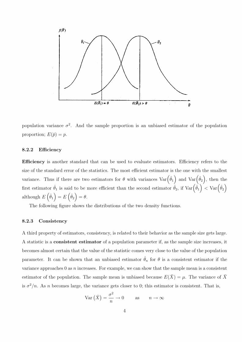
The following figure shows the sampling distributions of two estimators, θ̂1 and θ̂2. θ̂1 is an
unbiased estimator and θ̂2 a biased estimator. The following figure indicates that E(θ̂1) = θ
and E(θ̂2) > θ.
In general, unbiasedness is a desirable property for an estimator. The sample mean is an
unbiased estimator of the population mean because the mean of the sampling distribution of X̄,
E(X̄), is equal to the population mean µ. Similarly, the sample variance is an unbiased estimator
of the population variance because the mean of the sample distribution of s2, E(s2), is equal to
3
population variance σ2. And the sample proportion is an unbiased estimator of the population
proportion; E(p̄) = p.
8.2.2 Efficiency
Efficiency is another standard that can be used to evaluate estimators. Efficiency refers to the
size of the standard error of the statistics. The most efficient estimator is the one with the smallest
variance. Thus if there are two estimators for θ with variances Var(
θ̂1
)
and Var(
θ̂2
)
, then the
first estimator θ̂1 is said to be more efficient than the second estimator θ̂2, if Var(
θ̂1
)
< Var(
θ̂2
)
although E(
θ̂1
)
= E(
θ̂2
)
= θ.
The following figure shows the distributions of the two density functions.
8.2.3 Consistency
A third property of estimators, consistency, is related to their behavior as the sample size gets large.
A statistic is a consistent estimator of a population parameter if, as the sample size increases, it
becomes almost certain that the value of the statistic comes very close to the value of the population
parameter. It can be shown that an unbiased estimator θ̂n for θ is a consistent estimator if the
variance approaches 0 as n increases. For example, we can show that the sample mean is a consistent
estimator of the population. The sample mean is unbiased because E(X̄) = µ. The variance of X̄
is σ2/n. As n becomes large, the variance gets closer to 0; this estimator is consistent. That is,
Var(
X̄)
=σ2
n→ 0 as n → ∞
4

8.3 Interval Estimates
• An Interval Estimate
An interval is constructed around the point estimate, and it is stated that this interval is likely
to contain the corresponding population parameter. Interval estimates indicate the precision, or
accuracy, of an estimate and are therefore preferable.
• Confidence Level and Confidence Interval
5
Each interval is constructed with regard to a given confidence level and is called a confidence
interval. The confidence level associated with a confidence interval states how much confidence
we have that this interval contains the true population parameter. The confidence level is denoted
by (1 − α)100%. When expressed as probability, it is called the confidence coefficient and is
denoted by 1 − α.
Although any value of the confidence level can be chosen to construct a confidence interval, the
more common values are 90%, 95%, and 99%. The corresponding confidence coefficients are 0.90,
0.95, and 0.99.
8.4 Interval Estimation of a Population Mean: Known Variances
Recall that in the case of X̄, the sample size is considered to be large when n is 30 or larger.
According to the central limit theorem, for a large sample the sampling distribution of the sample
mean X̄ is (approximately) normal irrespective of the shape of the population from which the sample
is drawn. Therefore, when the sample size is 30 or larger, we will use the normal distribution to
construct a confidence interval for µ.
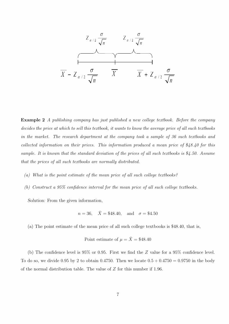
Confidence Interval for population mean µ
The (1 − α)100% confidence interval for µ is
X̄ ± Zα/2
σ√n
where X̄ is sample mean
σ is population standard deviation
n is the sample size
Zα/2 is read from the standard normal distribution table for the given confidence level.
Conditions: Normal population and Known variance
OR Nonnormal population, Large sample and Known variance
• Maximum Error of Estimate for µ
The maximum error of estimate for µ, denoted by E, is the quantity that is subtracted from
and added to the value of X̄ to obtain a confidence interval for µ. Thus,
E = Zα/2σX̄ = Zα/2
σ√n
6
Example 2 A publishing company has just published a new college textbook. Before the company
decides the price at which to sell this textbook, it wants to know the average price of all such textbooks
in the market. The research department at the company took a sample of 36 such textbooks and
collected information on their prices. This information produced a mean price of $48.40 for this
sample. It is known that the standard deviation of the prices of all such textbooks is $4.50. Assume
that the prices of all such textbooks are normally distributed.
(a) What is the point estimate of the mean price of all such college textbooks?
(b) Construct a 95% confidence interval for the mean price of all such college textbooks.
Solution: From the given information,
n = 36, X̄ = $48.40, and σ = $4.50
(a) The point estimate of the mean price of all such college textbooks is $48.40, that is,
Point estimate of µ = X̄ = $48.40
(b) The confidence level is 95% or 0.95. First we find the Z value for a 95% confidence level.
To do so, we divide 0.95 by 2 to obtain 0.4750. Then we locate 0.5 + 0.4750 = 0.9750 in the body
of the normal distribution table. The value of Z for this number if 1.96.
7

Next, we substitute all the values in the confidence interval formula for µ. The 95% confidence
interval for µ is
X̄ ± Zα/2
σ√n
= 48.40 ± 1.96 ×4.5√36
= 48.40 ± 1.47
= (48.40 − 1.47) to (48.40 + 1.47)
= $46.93 to $49.87
Thus, we are 95% confident that the mean price of all such college textbooks is between $46.93
and $49.87. Note that we cannot say for sure whether the interval $46.93 to $49.87 contains the
true population mean or not. Since µ is a constant, we cannot say that the probability is 0.95 that
this interval contains µ because either it contains µ or it does not. Consequently, the probability
is either 1.0 or zero that this interval contains µ. All we can say is that we are 95% confident that
the mean price of all such college textbooks is between $46.93 and $49.87.
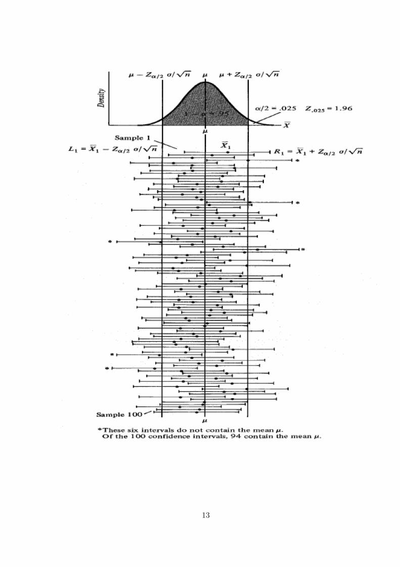
How do we interpret a 95% confidence level? In terms of the Example 2, if we take all possible
samples of 36 such college textbooks each and construct a 95% confidence interval for µ around
each sample mean, we can expect that 95% of these intervals will include and 5% will not.
Example 3 A study is being conducted in a company that has 1,800 engineers. A random sample of
50 of these engineers reveals that the average sample age is 34.3 years. Historically, the population
standard deviation of the age of the company’s engineers is approximately 8 years. Construct a 99%
confidence interval to estimate the mean age of all the engineers in this company.
8

Solution: From the given information,
n = 50, X̄ = 34.3 σ = 8,
and confidence level = 99% or 0.99.
Because the sample size is large (n > 30) and σ is known, by CLT, we will use the normal
distribution to determine the confidence interval for µ. To find Z for a 99% confidence level, we
divide 0.99 by 2 to obtain 0.4950. Thus, we locate 0.5 + 0.495 = 0.995 in the body of the normal
distribution. From the table, the Z value for 0.995 is approximately 2.58.
Substituting all the values in the formula, the 99% confidence interval for µ is
X̄ ± Zα/2
σ√n
= 34.3 ± 2.58 ×8√50
= 34.3 ± 2.9189 = 61.703 to 66.357
Thus, we can state with 99% confidence that the mean age of all the engineers in the company were
between 31.381 years and 37.219 years.
8.5 The Width of A Confidence Interval
The width of a confidence interval depends on the size of the maximum error ZσX̄ , which depends
on the values of Z, σ, and n because σX̄ = σ/√
n. However, the value of σ is not within the control
of the investigator. Hence, the width of a confidence interval depends on
1. The value of Z which depends on the confidence level
2. The sample size n
The confidence level determines the value of Z which in turn determines the size of the maximum
error. The value of Z increases as the confidence level increases, and it decrease as the confidence
level decreases.
For the same value of σ an increase in the sample size decreases the value of σX̄ , which in turn
decreases the size of the maximum error when the confidence level remains unchanged. Therefore,
an increase in the sample size decreases the width of the confidence interval. Thus, if we want to
decrease the width of a confidence interval, we have two choices:
1. Lower the confidence level
2. Increase the sample size
9

However, lowering the confidence level is not a good choice because a lower confidence level may
give less reliable results. Therefore, we should always prefer to increase the sample size if we want
to decrease the width of a confidence interval.
• Confidence Level and the Width of Confidence Interval
Example 4 Reconsider Example 2. Suppose all the information given in that example remains
the same. First, let us decrease the confidence level to 90%. From the normal distribution table,
Z = 1.65 for a 90% confidence level. Then, using Z = 1.65 in the confidence interval for µ, we
obtain:
X̄ ± Zα/2
σ√n
= 48.40 ± 1.65 ×4.5√36
= 48.40 ± 1.24
= $47.16 to $49.64
Comparing this confidence interval to the one obtained in Example 2, we observe that the width of
the confidence interval for a 95% confidence level is wider than the one for a 90% confidence level.
• Sample Size and the Width of Confidence Interval
Example 5 Consider Example 2 again. Now suppose the information given in that example is
based on a sample size of 160. Further assume that all other information given in that example,
including the confidence level, remains the same. Then, the 95% confidence interval for µ is
X̄ ± Zα/2
σ√n
= 48.40 ± 1.96 ×4.5√160
= 48.40 ± 0.70
= $47.70 to $49.10
Comparing this confidence interval to the one obtained in Example 2, we observe that the width of
the 95% confidence interval for n = 160 is smaller than the 95% confidence interval for n = 36.
8.6 Interval Estimation of a Population Mean: Unknown Variances
If the sample size is small, the normal distribution can still be used to construct a confidence interval
for µ if (1) the population from which the sample is drawn is normally distributed, and (2) the value
10
of σ is known. But more often we do not know σ and, consequently, we have to use the sample
standard deviation s as an estimator of σ. In such cases, the normal distribution cannot be used
to make confidence intervals about µ. When (1) the population from which the sample is selected
is (approximately) normally distributed, and (2) the population standard deviation σ is not known,
the normal distribution is replaced by the t distribution to construct confidence intervals about µ.
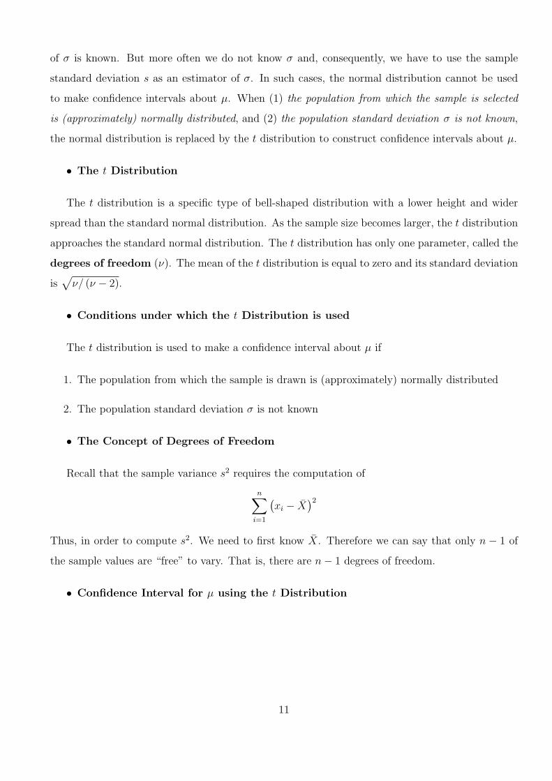
• The t Distribution
The t distribution is a specific type of bell-shaped distribution with a lower height and wider
spread than the standard normal distribution. As the sample size becomes larger, the t distribution
approaches the standard normal distribution. The t distribution has only one parameter, called the
degrees of freedom (ν). The mean of the t distribution is equal to zero and its standard deviation
is√
ν/ (ν − 2).
• Conditions under which the t Distribution is used
The t distribution is used to make a confidence interval about µ if
1. The population from which the sample is drawn is (approximately) normally distributed
2. The population standard deviation σ is not known
• The Concept of Degrees of Freedom
Recall that the sample variance s2 requires the computation of
n∑
i=1
(
xi − X̄)2
Thus, in order to compute s2. We need to first know X̄. Therefore we can say that only n − 1 of
the sample values are “free” to vary. That is, there are n − 1 degrees of freedom.
• Confidence Interval for µ using the t Distribution
11

Confidence Interval for population mean µ
The (1 − α)100% confidence interval for µ is
X̄ ± tα/2,n−1
s√n
where X̄ is sample mean
s is sample standard deviation
n is the sample size
t is obtained from the t distribution table for n − 1 degrees of freedom
and the given confidence level.
Conditions: (1) Population is approximately normal distributed
(2) σ is not known
Example 6 Dr. Moore wanted to estimate the mean cholesterol level for all adult males living in
London. He took a sample of 25 adult males from London and found that the mean cholesterol
level for this sample is 186 with a standard deviation of 12. Assume that the cholesterol levels for
all adult males in London are (approximately) normally distributed. Construct a 95% confidence
interval for the population mean µ.
Solution: From the given information,
n = 25, X̄ = 186, s = 12,
and confidence level = 95% or 0.95.
To find the value of t we need to know the degrees of freedom and the area under the t distribution
curve in each tail.
Degrees of freedom = ν = n − 1 = 25 − 1 = 24
To find the area in each tail, we divide the confidence level by 2 . Thus,
Area in each tail = 0.5 − (0.95/2) = 0.5 − 0.4750 = 0.025
From the t distribution table, the value of t for ν = 24 and 0.025 area in the right tail is 2.0639.
12
13
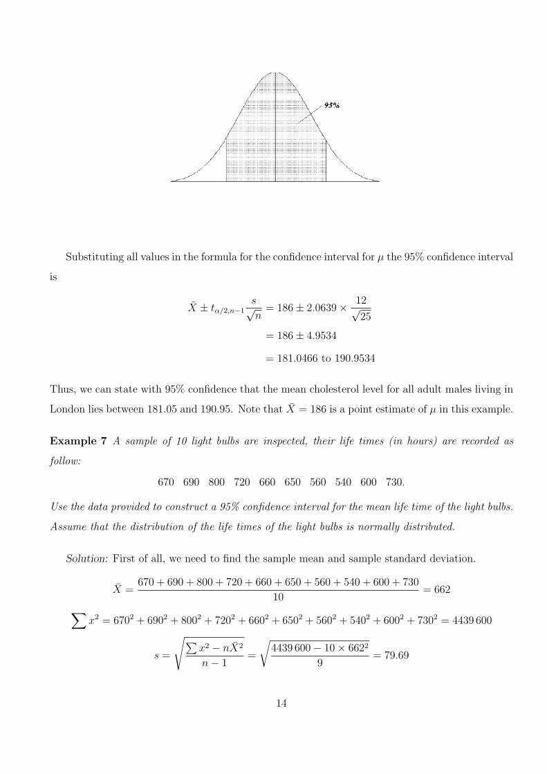
Substituting all values in the formula for the confidence interval for µ the 95% confidence interval
is
X̄ ± tα/2,n−1
s√n
= 186 ± 2.0639 ×12√25
= 186 ± 4.9534
= 181.0466 to 190.9534
Thus, we can state with 95% confidence that the mean cholesterol level for all adult males living in
London lies between 181.05 and 190.95. Note that X̄ = 186 is a point estimate of µ in this example.
Example 7 A sample of 10 light bulbs are inspected, their life times (in hours) are recorded as
follow:
670 690 800 720 660 650 560 540 600 730.
Use the data provided to construct a 95% confidence interval for the mean life time of the light bulbs.
Assume that the distribution of the life times of the light bulbs is normally distributed.
Solution: First of all, we need to find the sample mean and sample standard deviation.
X̄ =670 + 690 + 800 + 720 + 660 + 650 + 560 + 540 + 600 + 730
10= 662
∑
x2 = 6702 + 6902 + 8002 + 7202 + 6602 + 6502 + 5602 + 5402 + 6002 + 7302 = 4439 600
s =
√
∑
x2 − nX̄2
n − 1=
√
4439 600 − 10 × 6622
9= 79.69
14

Finally, from t-table, we find t0.025,9 = 2.2622. Thus, the 95% confidence interval is
X̄ ± ta/2,n−1
s√n
= 662 ± t0.025,979.69√
10
= 662 ± (2.2622)(25.25)
= 662 ± 57.121
= 604.879 to 719.121
8.7 Interval Estimation of a Population Proportion: Large Samples
Recall that the population proportion is denoted by p and the sample proportion is denoted by p̄.
The sample proportion p̄ is a sample statistic, and it possesses a sampling distribution. For large
samples:
1. The sampling distribution of the sample proportion p̄ is (approximately) normal.
2. The mean µp̄ of the sampling distribution of p̄ is equal to the population proportion p.
3. The standard deviation σp̄ of the sampling distribution of the sample proportion p̄ is√
p (1 − p) /n.
When estimating the value of a population proportion, we do not know the values of p and 1−p.
Consequently, we cannot compute σp̄. Therefore, in the estimation of a population proportion, we
use the value of sp̄ as an estimate of σp̄. The value of sp̄ is calculated using the following formula.
• Estimator of the Standard Deviation of p̄
The value of sp̄ which gives a point estimate of σp̄ is calculated as
sp̄ =
√
p̄ (1 − p̄)
n.
Because the sample proportion p̄ is the point estimator of the corresponding population proportion
p.
Confidence Interval for the Population Proportion p
The (1 − α)100% confidence interval for p is
p̄ ± Zα/2
√
p̄ (1 − p̄)
n
The value of Z used here is obtained from the standard normal distribution table
for the given confidence level
Conditions: np̄ ≥ 5 and n (1 − p̄) ≥ 5
15
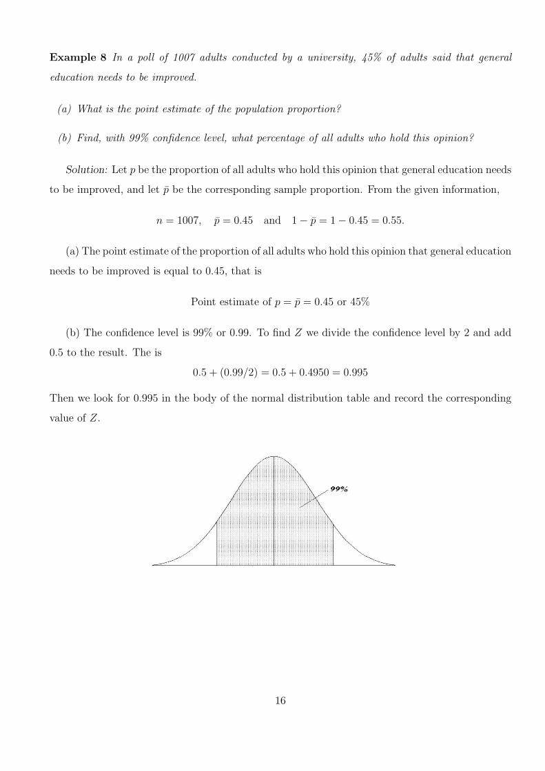
Example 8 In a poll of 1007 adults conducted by a university, 45% of adults said that general
education needs to be improved.
(a) What is the point estimate of the population proportion?
(b) Find, with 99% confidence level, what percentage of all adults who hold this opinion?
Solution: Let p be the proportion of all adults who hold this opinion that general education needs
to be improved, and let p̄ be the corresponding sample proportion. From the given information,
n = 1007, p̄ = 0.45 and 1 − p̄ = 1 − 0.45 = 0.55.
(a) The point estimate of the proportion of all adults who hold this opinion that general education
needs to be improved is equal to 0.45, that is
Point estimate of p = p̄ = 0.45 or 45%
(b) The confidence level is 99% or 0.99. To find Z we divide the confidence level by 2 and add
0.5 to the result. The is
0.5 + (0.99/2) = 0.5 + 0.4950 = 0.995
Then we look for 0.995 in the body of the normal distribution table and record the corresponding
value of Z.
16

The Z value for 0.995 is approximately 2.58 from the normal distribution table. Substituting
all the values in the confidence interval formula for p we obtain:
p̄ ± Zα/2
√
p̄ (1 − p̄)
n= 0.45 ± 2.58 ×
√
(0.45) (0.55)
1007
= 0.45 ± 0.041
= 0.409 to 0.491 or 40.9% to 49.1%
Thus, we can state with 99% confidence that the proportion of all adults who hold the opinion that
general education needs to be improved is between 0.409 to 0.491. The confidence interval can be
converted to a percentage interval as 40.9% to 49.1%.
Example 9 A sample of 20 managers was taken, and they were asked whether or not they usually
take work home. The responses of these managers are given below where YES indicates they usually
take work home and No means they do not.
Y es Y es No No No Y es No No
No No Y es Y es No Y es Y es No
No No No Y es
Make a 90% confidence interval for the percentage of all managers who take work home.
Solution: Let p be the percentage of all managers who take work home and let p̄ be the corre-
sponding sample proportion. From the given information,
n = 20 and p̄ =8
20= 0.4
Note that np̄ and n (1 − p̄) are both greater than 5. Consequently the sampling distribution of p̄ is
approximately normal, and we will use the normal distribution to calculate the margin of error for
the point estimate of p and to make a confidence interval about p.
The confidence level is 90% or 0.90. To find Z, we divide the confidence level by 2 and add 0.5
to the result. That is,
0.5 + (0.90/2) = 0.5 + 0.4500 = 0.95
The we look for 0.95 in the body of the normal distribution table and record the corresponding
value of Z. The Z value for 0.95 is approximately 1.65 from the normal distribution table.
17

Substituting all the values in the confidence interval formula for p, we obtain:
p̄ ± Zα/2
√
p̄ (1 − p̄)
n= 0.4 ± 1.65 ×
√
0.4 (1 − 0.4)
20
= 0.4 ± 0.1807
= 0.2913 to 0.5807 or 21.93% to 58.07%
Thus, we can state with 90% confidence that 21.93% to 58.07% of all managers take work home.
8.8 Sample Size Determination for the Estimation of Mean
One reason why we usually conduct a sample survey and not a census is that almost always we
have limited resources at our disposal. In light of this, if a smaller sample can serve our purpose,
then we will be wasting our resources by taking a larger sample. For instance, suppose we want to
estimate the mean life of a certain auto battery. If a sample of 40 batteries can give us the type of
confidence interval that we are looking for, then we will be wasting money and time if we take a
sample of a much larger size, say 500 batteries. In such cases, if we know the confidence level and
the width of the confidence interval that we want, then we can find the (approximate) size of the
sample that will produce the required result.
Recall that E = Zα/2σX̄ , is called the maximum error of estimate for µ. As we know, the
standard deviation σX̄ ; of the sample mean X̄ is equal to σ/√
n. Therefore, we can write the
maximum error of estimate for µ as
E = Zα/2
σ√n
If σ is unknown, we can use equation in above provided we have a planning value for σ. In
practice, one of the following procedures can be chosen.
1. Use the estimate of the population standard deviation computed from data of previous studies
as the planning value for σ.
2. Use a pilot study to select a preliminary sample. The sample standard deviation from the
preliminary sample can he used as the planning value for σ.
3. Use judgment or a “best guess” for the value of σ. The range divided by 4 is often suggested
as a rough approximation of the standard deviation and thus an acceptable planning value
for σ. That is,
σ ≈Range
4=
largest value − smallest value
4
18

• Determining the Sample Size for the Estimation of µ
Given the confidence level and the standard deviation of the population, the sample size that
will produce a predetermined maximum error E of the confidence interval estimate of µ is
n =Z2
α/2σ2
E2
If we do not know σ, we can take a preliminary sample (of any arbitrarily determined size) and find
the sample standard deviation s. Then we can use s for σ in the formula.
However, note that using s for σ may give a sample size that eventually may produce an error
much larger (or smaller) than the predetermined maximum error. This will depend on how close s
and σ are.
Example 10 Suppose the Census and Statistics department wants to estimate the mean family size
for all families in Hong Kong at a 99% confidence level. It is known that the standard deviation σ
for the sizes of all families in Hong Kong is 0.6. How large a sample should the department select
if it wants its estimate to be within 0.01 of the population mean?
Solution: The Census and Statistic department wants the 99% confidence interval for the mean
family size to be
X̄ ± 0.01
Hence, the maximum size of the error of estimate is to be 0.01, that is
E = 0.01
The value of Z for a 99% confidence level is 2.58. The value of σ is given to be 0.6. Therefore,
substituting all values in the formula and simplifying
n =Z2
α/2σ2
E2=
(2.58)2(0.6)2
(0.01)2=
(6.6564)(0.36)
(0.0001)= 23963.04 ≃ 23, 964.
Thus, the required sample size is 23,964. If the Census and Statistic department takes a sample of
23,964 families, computes the mean family size for this sample, and then constructs a 99% confidence
interval around this sample mean, the maximum error of the estimate will be approximately 0.01.
Note that we have rounded the final answer for the sample size to the next higher integer. This is
always the case when determining the sample size.
19
8.9 Sample Size Determination for the Estimation of Proportion
Just as we did with the mean, we can also determine the sample size for estimating the population
proportion p. This sample size will yield an error of estimate that may not be larger than a
predetermined maximum error. By knowing the sample size that can give us the required results,
we can save our scarce resources by not taking an unnecessarily large sample. The maximum error
E of the interval estimation of the population proportion is
E = Zα/2
√
p (1 − p)
n
• Determining the Sample Size for the Estimation of p
Given the confidence level and the values of p and 1 − p, the sample size that will produce a
predetermined maximum error E of the confidence interval estimate of p is
n =p (1 − p) Z2
α/2
E2
We can observe from this formula that to find n, we need to know the values of p and 1 − p.
However, the values of p and 1 − p are not known to us. In such a situation, we can choose one of
the following alternatives.
1. We make the most conservative estimate of the sample size n by using p = 0.50 and 1 − p =
0.50. For a given E, these values of p and 1 − p will give us the largest sample size by
comparison to any other pair of values of p and 1 − p because the product of p = 0.50 and
1 − p = 0.50 is greater than the product of any other pair of values for p and 1 − p.
n =0.25 × Z2
α/2
E2
2. We take a preliminary sample (of arbitrarily determined size) and calculate p̄ and (1 − p̄) for
this sample. Then, we use these values of p̄ and (1 − p̄) as p and (1 − p) to find n.
n =p̄ (1 − p̄) Z2
α/2
E2
20
Example 11 An Electronics Company has just installed a new machine that makes a part that
is used in clocks. The company wants to estimate the proportion of these parts produced by this
machine that are defective. The company manager wants this estimate to be within 0.02 of the
population proportion for a 95% confidence level. What is the most conservative estimate of the
sample size that will limit the maximum error to within 0.02 of the population proportion?
Solution: The company manager wants the 95% confidence interval to be
p̄ ± 0.02
Therefore, E = 0.02. The value of Z for a 95% confidence level is 1.96. For the most conservative
estimate of the sample size, we will use p = 0.50 and 1− p = 0.50. Hence, the required sample size
is
n =0.25 × Z2
α/2
E2=
0.25 × (1.96)2
(0.02)2=
0.25 × 3.8416
(0.02)2= 2401
Thus, if the company takes a sample of 2401 parts, the estimate of p will be within 0.02 of the
population proportion.
Example 12 Consider the last example again. Suppose a preliminary sample of 200 parts produced
by this machine showed that 7% of them are defective. How large a sample should the company select
so that the 95% confidence interval for p is within 0.02 of the population proportion?
Solution: Again, the company wants the 95% confidence interval for p to be
p̄ ± 0.02
Hence, E = 0.02. The value of Z for a 95% confidence level is 1.96. From the preliminary sample,
p̄ = 0.07 and (1 − p̄) = 1 − 0.07 = 0.93.
Using these values of p̄ and (1 − p̄) as estimates of p and 1 − p, we obtain:
n =p̄ (1 − p̄) Z2
α/2
E2=
(0.07)(0.93)(1.96)2
(0.02)2=
(0.07)(0.93)(3.8416)
(0.0004)= 625.22 ≃ 626
Thus, if the company takes a sample of 626 items, the estimate of p will be within 0.02 of the
population proportion. However, we should note that this sample size will produce the maximum
error within 0.02 points only if p̄ is 0.07 or less for the new sample. But if p̄ for the new sample
happens to be much higher than 0.07, the maximum error will not be within 0.02.
Therefore, to avoid such a situation, we may be more conservative and take a much larger sample
than 626 items.
21