State and Ore Hardness Estimation inSemiautogenous Grinding ?

Alejandro Cuevas ∗ Aldo Cipriano ∗

∗ Department of Electrical Engineering,Pontificia Universidad Catolica de Chile, Santiago, Chile

(e-mail: agcuevas@ing.puc.cl, aciprian@ing.puc.cl)

Abstract: Semiautogenous milling is difficult to control both because of its non-linearbehavior and the effects of overloading due to increases in the ore charge or variations in orecharacteristics. Advanced control strategies and operational change detection methods are thusin need of strengthening using techniques such as state estimation. Non-linear state estimationis a complex task for which various solutions have been proposed, such as the extended Kalmanfilter, the particle filter and the moving horizon estimator. In this study we present firstly aquantitative comparison of these solutions using a dynamic model validated with mill data. Theresults indicate that in addition to its lower computational requirements, the extended Kalmanfilter delivers the best performance in robustness and estimation error. Next, we propose amethod for estimation of changes in the hardness of the ore feed that we test by simulation.Finally, we show that this method also works with real data.

Keywords: Semiautogenous grinding; State estimation; Extended Kalman filter; Particle filter;Moving horizon estimation; Genetic algorithms.

1. INTRODUCTION

Semiautogenous milling, one of the most widely usedmethods of ore concentration, involves the feeding of largerock particles and water into a grinding mill containingsteel balls that rotates at approximately 75% of its criticalspeed. The slurry and ball charge adheres to the wallsof the mill before cascading off at a given angle, causingimpact and fragmenting the ore. This process exhibitssignificant non-linearities and can be adversely affectedby mill overload, whether caused by an excess of ore orvariations in its hardness or granulometry. In response,various advanced control algorithms have been developedto achieve a more robust operation of the process in theface of such variations or changes in the ore feed (Sbarbaroet al., 2005).

Advanced control and operational change detection sys-tems generally employ process models. The most de-veloped versions use relatively simple structures whoseparameters are identified on the basis of input-outputdata. Others attempt to model the phenomenology ofthe process, but these are more complex designs basedon fracture kinetics whose parameters include grindingand discharge rates (Austin, 1997). Although such modelscan reproduce the interactions between the variables moreaccurately, they require a non-linear state estimator for usein control or fault detection and diagnosis. Various solutionalternatives are available for state estimation in non-linearsystems, and their suitability must be evaluated case bycase. In (Herbst et al., 1980), for example, a derivationof the Kalman filter known as the extended Kalman filter

? This work was supported by Fondecyt Project No. 1050684 andthe Pontificia Universidad Catolica de Chile

(EKF) is utilized in ball mill applications. More recentproposals include the use of particle filters (Arulampalamet al., 2002) and moving horizon estimation (Rao et al.,2003) for general application.

In this work we compare the three above-mentioned esti-mation methods using a dynamic semiautogenous grindingmodel developed in (Amestica et al., 1996) and (Gonzalezet al., 2006). The model was validated with operatingdata from a pilot plant. Our first objective is to comparestate estimators on the grinding plant model. Our secondobjective is to identify hardness variations in the ore feedin real time. For these purposes we assume the presence ofsensors that measure power consumption and total chargeweight, from which we can deduce the discharge flow ofwater and ore. Input measurements are total ore feed flow,feed water flow and the ore’s granulometric distribution.

2. DYNAMIC MODEL

The basic elements of a semiautogenous (SAG) mill area grinding chamber, a discharge module and slurry trans-port, as depicted by the block diagram in figure 1. The orefeed is represented by vector f , whose components expressthe ore flow by size. Fa indicates the feed water flow.

The grinding chamber is a rotating cylinder where the ac-tual grinding takes place both through collisions betweenthe ore particles and the impact of the steel balls. BlockC in figure 1 is a classifier consisting of a grate and apulp lifter that distributes the slurry into flows either forimmediate discharge or recirculation to the chamber andfurther grinding. The dynamic model of the mill we willemploy here is the one given in (Amestica et al., 1996). Itconsists of the following variables and parameters:

Proceedings of the 17th World CongressThe International Federation of Automatic ControlSeoul, Korea, July 6-11, 2008

978-1-1234-7890-2/08/$20.00 © 2008 IFAC 3310 10.3182/20080706-5-KR-1001.3553

Fig. 1. Block diagram of SAG system.

• Variablesfi,Fa: Ore feed flow by size class, feed water flow.

FM : Total mass flow.wi,WA: Ore mass by size interval, water mass.

WM : Total ore mass inside mill chamber.pi,PA: Discharge mass flow by size class, water flow.

PM : Total ore mass flow.f∗i : Ore mass flow by size class entering mill chamber.p∗i : Discharge mass flow by size class exiting mill chamber.ri: Ore mass flow by size class for internal recirculation.J : Load fraction of mill chamber.

Mp: Mill power consumption.

• ParametersK: Ore grinding rate by size class.C: Classification efficiency at discharge grate.

P ∗: Internal mass flow.γA: Water discharge rate.

All flows are measured in T/h and masses in T . Mill poweris measured in kW .

The equations defining the model are categorized intogrinding (1), transport (2) and classification equations (3):

dWi+1

dt= Kiwi+1 (1)

p∗i =P ∗

Wmwi (2)

ri =P ∗

WmCwi ; pi =

P ∗

Wm(In − C)wi (3)

Parameters γA and P ∗ vary with time and are obtainedfrom measurements while matrices K and C are derivedfrom a probability distribution of the reduction and clas-sification phenomena (Austin, 1997). Parameters γA andP ∗ satisfy the following relationships:

γA = r +s

W 4m

; P ∗ = q√Wm (4)

where r, s and q are calibration parameters.

The dynamic model synthesizing mill operation takes intoaccount the steel balls that increase the effectiveness ofthe grinding process. In simplified models, the grindingphenomena that reduce particle size can be representedby a single parameter known as the effective ore grindingrate K. If we denote the ore mass greater than size di inthe chamber as Wi+1, and if Ki is the effective grindingrate for ore of size di, we have the grinding relationshipgiven by (1).

Power consumption and load fraction variables are closelyrelated. For the mill we are modeling, load fraction (from 0to 1) has been found experimentally to satisfy the followingrelationship:

J = aWm + b (5)

where Wm is derived from the density and porosity of theore. The additive constant Wb represents the volume ofthe steel balls.

As for power consumption, it is given by the mill parame-ters and the total mass inside the chamber:

Mp = (mJ + c) (W −m+WA +Wb) (6)

Coefficients a, b, m and c are also calibration parameters.All parameters values are displayed in Table 1.

Table 1: Calibration parameters of models.

a b m c r s q Wb T

0.407 0.0723 -24.3 18.6 16.86 0.102 29 0.52

The equations given above are combined in the stateequations as:dwi

dt= − 1

Wm

[P ∗ (In − C ′) +MpR

−1KeR]wi + fi (7)

dWA

dt= −γAWA + FA (8)

where i is the ore size class index, C ′ is defined to includethe recirculation flow and Ke is the specified grinding raterelated to power consumption Mp. R is a ones and zerosmatrix wich relates wi with Wi. The outputs defined in themodel can be measured or inferred from operation dataand are given by:

pi =P ∗

Wm(In − C)wi

PM =n∑

i=1

P ∗

Wm(In − C)wi (9)

PA = γAWA

This base model incorporates n = 26 size classes and wascalibrated with data obtained from a pilot plant run byCodelco (Amestica et al., 1996).

3. SIMULATION

The simulation was carried out in Simulink. Since themodel is continuous, it was discretized using ∆t = 10 s asa step in its integration, with (7),(8) as the state functionsand (9) as the output function in their discretized forms.The initial operating conditions were 8.4 T/h for total orefeed flow (4.2 T/h hard and 4.2 T/h soft ore) and 1.2 T/hwater feed flow.

Figure 2 shows the trend over time of hold-up mass andmill power consumption over a period of 5 h. Total feedflow was increased by 25% at t = 2 h, the ore fines propor-tion was varied from 80% to 95% at t = 3 h, and finally,soft ore was varied from 60% to 20% at t = 4 h. Notethat an increase in total feed flow leads to a rise in totalhold-up mass and therefore also in power consumption.If the total charge exceeds a certain threshold, the mill

17th IFAC World Congress (IFAC'08)Seoul, Korea, July 6-11, 2008

3311

Fig. 2. Variation over time of hold-up mass and powerdue to changes in tonnage (a), granulometry (b) andhardness (c) of mill feed.

chamber becomes overloaded and breakage declines dueto the excess ore, thus lowering the mill’s power draw. If,on the other hand, the proportion of fines increases, boththe load and the draw diminish due to the greater ease ofore evacuation. Finally, a lower soft ore proportion impliesless breakage and therefore lower ore evacuation, thusincreasing both load and power draw. For these reasons,a linear filter could not show satisfactory results as nonlinear estimations shown in the next section.

4. STATE ESTIMATION

We now turn to the quantitative comparisons of thethree state estimation solutions, they being the extendedKalman filter (Welch and Bishop, 2004), the particlefilter (Arulampalam et al., 2002) and the moving horizonestimator (Rao et al., 2003).

For the extended Kalman filter (EKF), we used matricesQ and R , both dimension 5 × 5, which are equal to theidentity matrix multiplied by a scalar for all states, whichrepresents typical sensor noise or process noise. In the caseof the particle filter (PF) we utilized Np = 20, becausebetter results didnt appear with larger number of particles.Finally, for the moving horizon estimator (MHE) a horizonof 5 and a time estimation step ∆t = 50 were employed.Genetic algorithms were applied to solve the optimizationproblem, with 10 generations of 30 individuals initiallydistributed uniformly. The results of the search were thenused as the starting solution in a classic optimizationalgorithm. A simplified version of the model was employedusing the same structure but only five states: coarse-hardw1, coarse-soft w2, fine-hard w3, fine-soft w4, and waterWA.

dw1

dt=−G1Mp

Wmw1 + (1− α) (1− β)Fm + δw1

dw2

dt=−G2Mp

Wmw2 + α (1− β)Fm + δw2

dw3

dt=−Pm1 +

G1Mp

Wmw1 + (1− α)βFm + δw3 (10)

dw4

dt=−Pm2 +

G2Mp

Wmw2 + αβFm + δw4

dWA

dt=−γAWA + FA + δWA

Where δw1, δw2, δw3, δw4, δWA are process noises oftheir respective state variables. G1 is hard ore’s hardnessand G2 is soft ore’s hardness. Values of G1 = 0.1 T/kJand G2 = 0.2 T/kJ are used, which represent averagesfor K matrix values for soft mineral and hard mineral,respectively.

Parameter β is defined as the ore fines mass flow propor-tion with respect to the total feed mass flow. Parameter αis defined as soft ore mass flow proportion with respect tothe same total. Thus, α = 0 indicates that the feed includesonly hard ore, α = 1 means it contains only soft ore andα = 0.5 designates equal proportions of both. Therefore,α represents the overall hardness of the system in a singleparameter.

The performance of the three estimators is summarized inTables 2, 3 and 4 for the various operating scenarios. RootMean Square Errors from the estimations are shown for thefollowing ore variables: coarse (w1 + w2), fine (w3 + w4),hard (w1 + w3), and soft (w2 + w4). Table 2 gives theresults for normal operating conditions, with total ore feedof 7 T/h, feed water flow of 1.2 T/h, fines proportionβ = 0.8 and soft ore proportion α = 0.5. In Table 3, weagain have α = 0.5, total ore feed of 7 T/h and feed waterflow of 1.2 T/h, but β = 0.9. At t = 2 h total ore feed wasincreased 10%, and at t = 4 h, ore fines β were increasedfrom 90% to 95% of feed flow. The operating conditionsfor Table 4 are normal with the exception that 10% morefeed water flow was added at t = 2 h.

Table 2: RMSE in T for estimates under normaloperating conditions.

Coarse Fine Hard Softw1 + w2 w3 + w4 w1 + w3 w2 + w4

EKF 0.0060 0.0081 0.0107 0.0028

PF 0.0082 0.0069 0.0072 0.0034

MHE 0.0162 0.0111 0.0370 0.0212

Table 3: RMSE in T for estimates with changes intonnage and granulometry.

Coarse Fine Hard Softw1 + w2 w3 + w4 w1 + w3 w2 + w4

EKF 0.0053 0.0064 0.0162 0.0124

PF 0.0081 0.0069 0.0071 0.0032

MHE 0.0026 0.0131 0.0075 0.0094

Table 4: RMSE in T for estimates with changes in feedwater flow.

Coarse Fine Hard Softw1 + w2 w3 + w4 w1 + w3 w2 + w4

EKF 0.0059 0.0082 0.0108 0.0028

PF 0.0114 0.0080 0.0108 0.0050

MHE 0.0159 0.0113 0.0367 0.0211

Figures 3, 4 and 5 graph the variation over time of the stateand state estimates. The operation conditions are the sameas in Table 3. The estimations are implemented using (10)as a simplified model of the 26 states model from which themeasures are obtained. Initial estimations are 0.05 T forcoarse, 0.15 T for fine, hard and soft, picked as a normaloperation. The tests reveal that the estimators generallybehave well in the face of various types of disturbancesrelative to normal operation, with EKF and PF givingsimilar results and MHE slightly worse. They do not seemto be strongly affected by operating changes, and thus

17th IFAC World Congress (IFAC'08)Seoul, Korea, July 6-11, 2008

3312

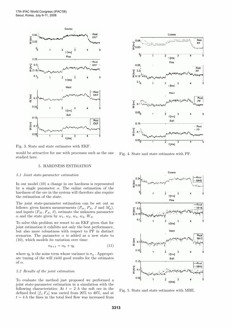
Fig. 3. State and state estimates with EKF.

would be attractive for use with processes such as the onestudied here.

5. HARDNESS ESTIMATION

5.1 Joint state-parameter estimation

In our model (10) a change in ore hardness is representedby a single parameter α. The online estimation of thehardness of the ore in the system will therefore also requirethe estimation of the state.

The joint state-parameter estimation can be set out asfollows: given known measurements (Pm, PA, J and Mp),and inputs (FM , FA, β), estimate the unknown parameterα and the state given by w1, w2, w3, w4, WA.

To solve this problem we resort to an EKF given that forjoint estimation it exhibits not only the best performance,but also more robustness with respect to PF in distinctscenarios. The parameter α is added as a new state to(10), which models its variation over time:

αk+1 = αk + ηk (11)

where ηk is the noise term whose variance is ση . Appropri-ate tuning of the will yield good results for the estimatesof α.

5.2 Results of the joint estimation

To evaluate the method just proposed we performed ajoint state-parameter estimation in a simulation with thefollowing characteristics: At t = 2 h the soft ore in thedefined feed [fi, FA] was varied from 20% to 40%, and att = 4 h the fines in the total feed flow was increased from

Fig. 4. State and state estimates with PF.

Fig. 5. State and state estimates with MHE.

17th IFAC World Congress (IFAC'08)Seoul, Korea, July 6-11, 2008

3313

Fig. 6. State and joint state-parameter estimates withEKF.

90% to 95%. The state estimates results are displayed infigure 6 and the estimate of α is given in figure 7. Table 5contains the estimation errors for different variations in αassuming the other parameters are constant. The case offigure 7, where initial α is 0.2 and final α is 0.4, generatesan RMSE of 0.04.

Table 5: Error of parameter α.

α 0.1 0.2 0.3 0.4 0.5 0.6 0.7 0.8 0.9

0.1 0.17 0.16 0.06 0.05 0.12 0.08 0.10 0.11 0.14

0.2 0.16 0.10 0.03 0.04 0.07 0.07 0.10 0.11 0.13

0.3 0.16 0.05 0.02 0.03 0.06 0.06 0.11 0.11 0.15

0.4 0.15 0.05 0.04 0.03 0.04 0.07 0.13 0.15 0.42

0.5 0.54 0.41 0.42 0.24 0.03 0.06 0.13 0.12 0.13

0.6 0.58 0.41 0.41 0.23 0.05 0.08 0.14 0.13 0.14

0.7 0.48 0.45 0.43 0.27 0.07 0.07 0.07 0.06 0.07

0.8 0.60 0.46 0.43 0.26 0.05 0.07 0.05 0.04 0.04

0.9 0.66 0.48 0.42 0.26 0.13 0.06 0.04 0.03 0.02

The estimate of hardness using the state equations yieldssatisfactory results. The change in the proportion α wasestimated correctly in many cases. Table 5 shows thatapproximately 65% of all combinations performed satis-factorily.

6. EVALUATION USING REAL DATA

6.1 Estimation of parameter α

The solution given in Section 5, though it performs suc-cessfully, assumes we have at our disposal an appropriatelycalibrated phenomenological model of the process. In anactual industrial plant, however, a model of these charac-teristics is not necessarily available. As we will now show,even in such situations it is possible to apply the same

Fig. 7. Parameter α and α estimate.

concept of representing a change of hardness with a singleparameter.

We begin by assuming we have identified two models M1

andM2 of extreme hardness. Let us also suppose thatM1

and M2 present an ARMA model structure given by:M1 : A1(q)y(k) = B1(q)u(k − d) (12)M2 : A2(q)y(k) = B2(q)u(k − d) (13)

where A1, A2, B1, B2 are polynomials of orders na and nb

respectively, and q is an operator which represents a stepforward in time, and d the delay of the model. We canexpress the two models in regresion form as:

M1 : y(k) = φT1 (k)θ1 ; M2 : y(k) = φT

2 (k)θ2 (14)

where φT1 , φ

T2 and θ1, θ2 are the regresion and estimated

parameters vectors respectively. Let us now consider thecase where the mill operates at an intermediate hardness.The integrated model then becomes:

M0 : y(k) = αy1(k) + (1− α)y2(k) (15)

Where y1(k) and y2(k) are outputs of models M1 andM2 respectively. In order to determine parameter α, thefollowing cost function is minimized:

J(α) =N∑

k=1

(y(k)− αφT

1 (k)θ1 − (1− α)φT2 (k)θ2

)2

(16)

The optimal value α that minimizes (16) is given by:

α =

(N∑

k=1

ψ(k)ψ(k)T

)−1 N∑k=1

ψ(k)z(k) (17)

where ψ(k) and z(k) are given by:

ψ(k) = φT1 (k)θ1 − φT

2 (k)θ2 ; z(k) = y(k)− φT2 (k)θ2 (18)

One of the problems that arise in practice is to determinewhether the operating situation corresponds to an extremecase of hard or soft ore. For this we propose the use of theaverage power-tonnage ratio, which intuitively representshow difficult it is for the mill to fracture the ore.

6.2 Test with industrial plant data

For testing the estimation algorithm, three series of nor-malized data obtained from measurements of a given in-dustrial plant are used. Each series corresponds to plant

17th IFAC World Congress (IFAC'08)Seoul, Korea, July 6-11, 2008

3314

Fig. 8. Tonnage and speed inputs.

Fig. 9. Electric power and one step prediction of power.

operation on three different days. For the sake of simplicity,to identify the ARMA model, orders na = 1, nb = 1 andd = 0 are employed.

The first base model is defined as the series with thelowest power-tonnage ratio (α = 1), and the second basemodel as the series with the highest such ratio (α = 0).From the third series, corresponding to the intermediateratio, we use the first half to estimate parameter α, andthe second half for evaluating the prediction with theintegrated model. The error is evaluated by a one-stepprediction with a sample period of ∆t = 2. The signals arefiltered by averaging the last ten samples. Figures 8 and9 show the variation over time of the input and outputvariables, that is, tonnage set-point and mill speed, andelectric power, respectively. Upon estimation of parameterα we obtain α = 0.67, which indeed corresponds to anintermediate value between α = 0 and α = 1. For thisparameter, the integrated model of power gives an RMSEof 0.007, far below 0.95 which is the average value of thenormalized signal. The prediction obtained is shown infigure 9.

7. CONCLUSIONS AND FUTURE RESEARCH

The extended Kalman filter delivered similar state estima-tion results to the particle filter, although in some cases thelatter was less robust. As regards robustness with respectto disturbances and estimation error, the EKF was heavilydependent on the matrices Q and R. The performanceof the moving horizon estimator was acceptable, but wasless precise than EKF and PF and exhibited higher com-putational costs, with execution up to ten times more

time-consuming. This can be adjusted while maintainingreasonable results by changing certain parameters of thealgorithm thanks to the flexibility provided by the geneticalgorithms as an optimization tool.

The hardness estimation tests show that with a phenom-enological model of the system, an extended Kalman filterdelivers good results in a significant proportion of cases.Even in some of the cases with a relatively high error,the estimation still manages to detect the correct trendof the change in α. The approach based on summarizingthe effects of an operational change in a single parameteris also useful if a model is not available. In this case, avery low error prediction error was obtained, by using anARMA model.

As regards future research, the method presented herecould be extended to models higher order and to appli-cations other than semiautogenous grinding. The methodcould also be used in adaptive predictive control and infault diagnosis.

REFERENCES

R. Amestica, G. Gonzalez, J. Menacho and J. Barria. Amechanistic state equation model for a semiautogenousgrinding mill. International Journal of Mineral Process-ing, volume 44(45), pages 349–360, 1996.

S. Arulampalam, S. Maskell, N. Gordon and T. Clapp.A tutorial on particle filters for online non-linear/non-gaussian bayesian tracking. IEEE Tansactions on SignalProcessing, volume 50(2), pages 174–188, 2002.

L.G. Austin. Concepts in process design of mills, com-minution practices. Society for Mining, Metallurgy, andExploration, Inc., Littleton, Colorado, 1997.

G.D. Gonzalez, R. Paut, A. Cipriano, D. Miranda andG. Ceballos. Fault detection and isolation using con-catenated Wavelet Transform variances and discrimi-nant analysis. IEEE Tansactions on Signal Processing,volume 54(5), pages 1727–1736, 2006.

J.A. Herbst, K. Rajamani and W.T. Pate. Identificationof ore hardness disturbances in a grinding circuit using aKalman filter. Proceedings of the 3rd IFAC Symposiumon Automation in Mining, Mineral, and Metal Process-ing, Montreal, pages 333–348, 1980.

C. Rao, J. Rawlings and D. Mayne. Constrained state esti-mation for nonlinear discrete-time systems: stability andmoving horizon approximations. IEEE Transactions onAutomatic Control, volume 48(29), pages 246–258, 2003.

D. Sbarbaro, J. Barriga, H. Valenzuela and G. Cortes.A multi-input-single-output smith predictor for feederscontrol in SAG grinding plants. IEEE Transactions onControl Systems Technology, volume 13(6), pages 1069–1075, 2005.

G. Welch and G. Bishop. An introduction to the Kalmanfilter. University of North Carolina, Chapel Hill, NC,Tech. Rep. TR-95-041, 2004.

17th IFAC World Congress (IFAC'08)Seoul, Korea, July 6-11, 2008

3315