Mass_Spring_Damper Tutorial

ODE45 Function

ODE45 is used to solve linear or non-linear differential equations. This is done with a 4th and 5th order Runge-Kutta method to integrate the equations. NOTE - you DO NOT have to understand 4th and 5th order Runge-Kutta method to use ODE45 solver, check a numerical methods book if you are interested. You will only need to know the parameters to run the routine.

ODE45 has a typical form to use. tspan = [t_start, t_final]; X0 = [x0, xdot0]; options = odeset('Refine',6,'RelTol',1e-4,'AbsTol',1e-7); [T, X] = ode45(@F, tspan, X0, options); T in the left bracket is for time. X is our main variables, in vector form. F in the right side is a name of the subprogram for ODE45 solver which will be explained

in detail a little bit later). tspan is the time period that you want to calculate, which consists of start time and end time. X0 contains the initial conditions for ODE variable, x0 = x(0), xdot0 = xdot(0). options is the command that you can adjust the performance of ODE45 solver. There are many options you can choose from, type 'help odeset' at the Matlab command line. 'Refine' controls the number of data points for ODE solver. The higher the number after 'Refine' is more data points there are, but the slower the calculation is. 'RelTol' controls the relative error tolerance and 'AbsTol' controls the absolute error tolerances.

The following is an example of a pendulum problem which illustrates the use of ode45.

% % Matlab example program #4 % The first few lines are for constant input values like mass of the bar, etc. The numbers given are all arbitrary. m = 1; % mass of the bar g = 9.806; % acceleration of gravity l = 1; % length of the bar tspan = [0,5]; % time duration for calculation Now, plug in the initial conditions for main variable, theta in this case, the rotation angle of bar. theta = 1e-4; % initial displacement of the bar theta_dot = 0; % initial angular velocity of the bar

Note here there is a non-zero initial displacement (disturbance) and a zero initial velocity. x0 = [theta,theta_dot]; options = odeset('Refine',6,'RelTol',1e-4,'AbsTol',1e-7); % 'Refine' was used to produce good-looking plots % default value of Refine was 4. Tolerances were also tightened. % scalar relative error tolerance 'RelTol' (1e-3 by default) and % vector of absolute error tolerances 'AbsTol' (all components 1e-6 by % default).

'Refine' option does not apply if time span is more than 2. After we specify all the inputs for ODE45 solver, we write [t,x] = ode45(@pend_sol,tspan,x0,options);

% Note that the equations of motion in state space form are in a % subprogram named pend_sol

After finishing the calculation, you plot them. Here are some of the plotting commands.

figure(1); clf; plot(Theta*180/pi,Theta_dot,'b'); title('Pendulum problem'); xlabel('Displacement (degrees)'); ylabel('Angular velocity (radians/sec.)'); mx_theta_dot = max(Theta_dot); axis([0 360 0 1.1*mx_theta_dot]); grid;

Here, "pend_sol" is the name of the subprogram and it is shown below. You must create

a separate file for the subprogram with the same name you gave in the main program under the same folder/directory.

function xdot = pend_sol(t,x) % Constants and input variables g = 9.81; % gravity (m/s^2) l = 1; % length of the bar % State variables x_dot1 = x(2); x_dot2 = (3*g)/(2*l)*sin(x(1)); xdot = [x_dot1; x_dot2]; % end of subprogram.

The first line is for declaring the subprogram. Array xdot is for a derivative of array x, so xdot(1) is a derivative of x(1), an angular velocity and xdot(2) is an angular acceleration. You just write that down in the program as above. For a state space derivation tutorial

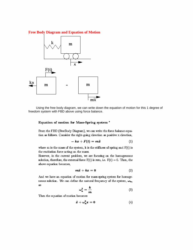
Free Body Diagram and Equation of Motion

Using the free body diagram, we can write down the equation of motion for this 1 degree of freedom system with FBD above using force balance.

Closed Form Solution

We can code the closed form solution into MATLAB. The following is the MATLAB code for closed form solution of mass-spring system. At the beginning of the program, we need to write some constant inputs. n is the number of the data points.

m = 1; % mass of the system in meter k = 50; % stiffness of the spring (N/m) wn = sqrt(k/m); % natural frequency (rad/sec) t_final = 2; % calculation time n = 500; % number of data points %Then, initial conditions are followed. x_0 = 1; % initial displacement x_dot_0 = 0; % initial velocity %Calculate the amplitude and the phase angle with given initial conditions. X_0 = sqrt(x_0^2+(x_dot_0/wn)^2); phi = acos(x_0/X_0); %And we can determine the displacement x(t) and velocity x_dot(t). t = 0:t_final/n:t_final; x = X_0*cos(wn*t+phi); % displacement x(t) x_dot = -wn*x_0*sin(wn*t+phi); % velocity x_dot(t)

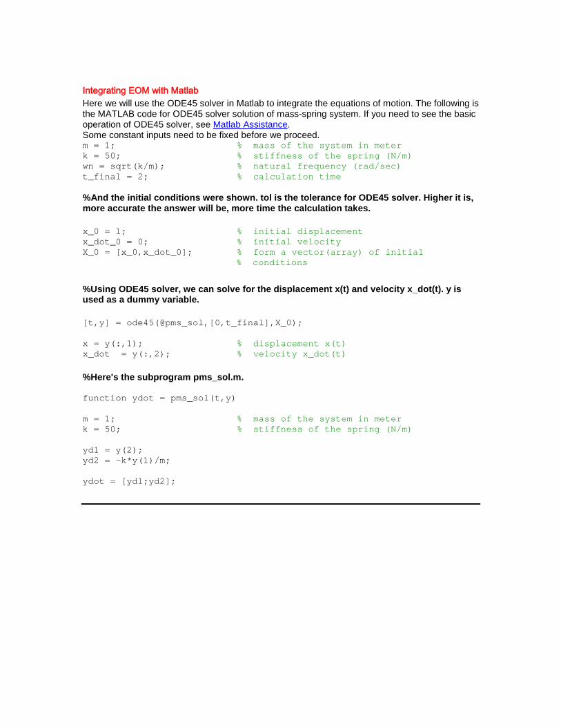
Integrating EOM with Matlab Here we will use the ODE45 solver in Matlab to integrate the equations of motion. The following is the MATLAB code for ODE45 solver solution of mass-spring system. If you need to see the basic operation of ODE45 solver, see Matlab Assistance. Some constant inputs need to be fixed before we proceed. m = 1; % mass of the system in meter k = 50; % stiffness of the spring (N/m) wn = sqrt(k/m); % natural frequency (rad/sec) t_final = 2; % calculation time %And the initial conditions were shown. tol is the tolerance for ODE45 solver. Higher it is, more accurate the answer will be, more time the calculation takes. x_0 = 1; % initial displacement x_dot_0 = 0; % initial velocity X_0 = [x_0,x_dot_0]; % form a vector(array) of initial % conditions %Using ODE45 solver, we can solve for the displacement x(t) and velocity x_dot(t). y is used as a dummy variable. [t,y] = ode45(@pms_sol,[0,t_final],X_0); x = y(:,1); % displacement x(t) x_dot = y(:,2); % velocity x_dot(t) %Here's the subprogram pms_sol.m. function ydot = pms_sol(t,y) m = 1; % mass of the system in meter k = 50; % stiffness of the spring (N/m) yd1 = y(2); yd2 = -k*y(1)/m; ydot = [yd1;yd2];

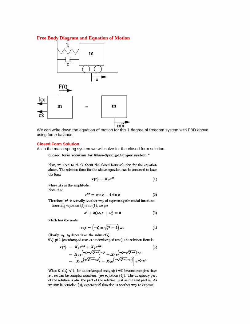
Free Body Diagram and Equation of Motion

We can write down the equation of motion for this 1 degree of freedom system with FBD above using force balance. Closed Form Solution As in the mass-spring system we will solve for the closed form solution.

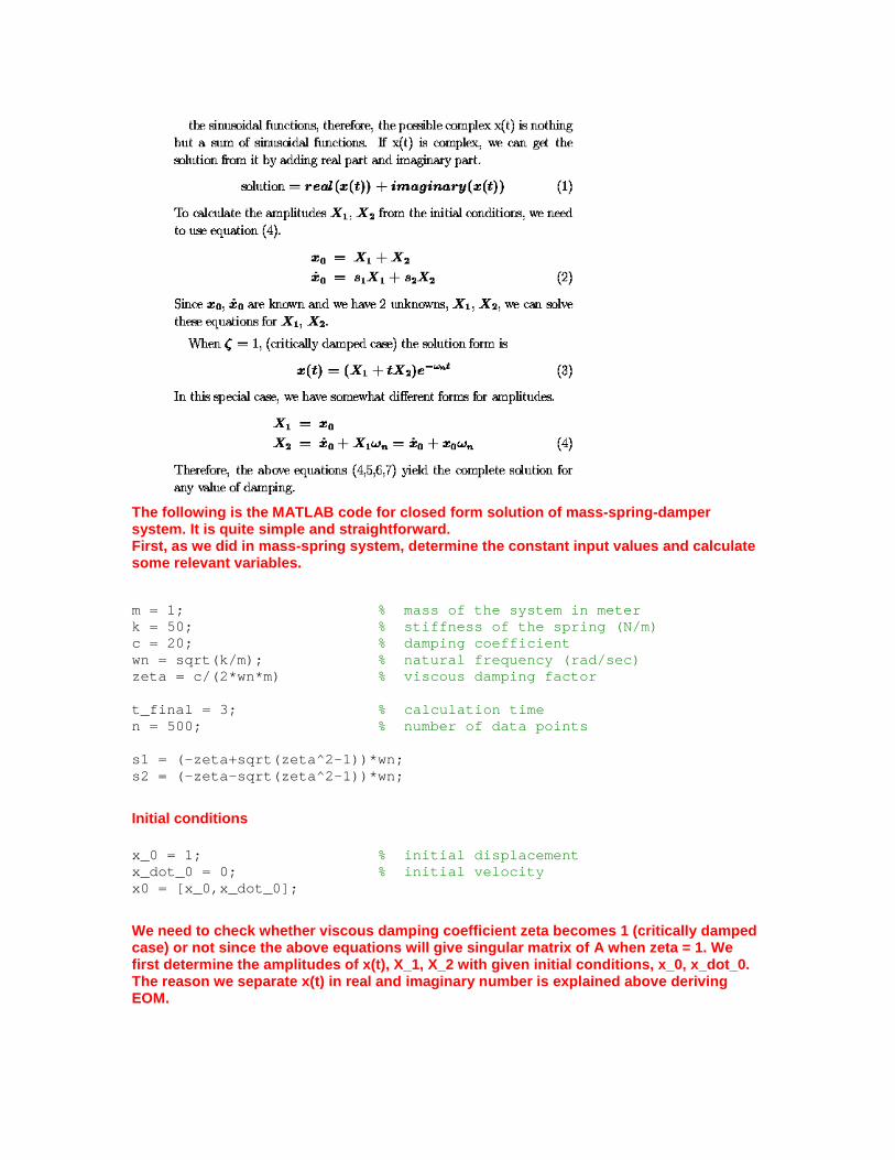
The following is the MATLAB code for closed form solution of mass-spring-damper system. It is quite simple and straightforward. First, as we did in mass-spring system, determine the constant input values and calculate some relevant variables. m = 1; % mass of the system in meter k = 50; % stiffness of the spring (N/m) c = 20; % damping coefficient wn = sqrt(k/m); % natural frequency (rad/sec) zeta = c/(2*wn*m) % viscous damping factor t_final = 3; % calculation time n = 500; % number of data points s1 = (-zeta+sqrt(zeta^2-1))*wn; s2 = (-zeta-sqrt(zeta^2-1))*wn;

Initial conditions x_0 = 1; % initial displacement x_dot_0 = 0; % initial velocity x0 = [x_0,x_dot_0];

We need to check whether viscous damping coefficient zeta becomes 1 (critically damped case) or not since the above equations will give singular matrix of A when zeta = 1. We first determine the amplitudes of x(t), X_1, X_2 with given initial conditions, x_0, x_dot_0. The reason we separate x(t) in real and imaginary number is explained above deriving EOM.

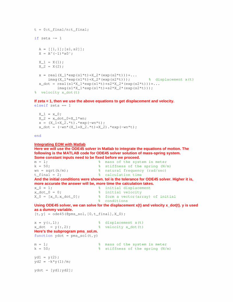
t = 0:t_final/n:t_final; if zeta ~= 1

A = [[1,1];[s1,s2]]; X = A^(-1)*x0'; X_1 = X(1); X_2 = X(2); x = real(X_1*exp(s1*t)+X_2*(exp(s2*t)))+... imag(X_1*exp(s1*t)+X_2*(exp(s2*t))); % displacement x(t) x_dot = real(s1*X_1*exp(s1*t)+s2*X_2*(exp(s2*t)))+... imag(s1*X_1*exp(s1*t)+s2*X_2*(exp(s2*t))); % velocity x_dot(t) If zeta = 1, then we use the above equations to get displacement and velocity. elseif zeta == 1 X_1 = x_0; X_2 = x_dot_0+X_1*wn; x = (X_1+X_2.*t).*exp(-wn*t); x_dot = (-wn*(X_1+X_2.*t)+X_2).*exp(-wn*t); end Integrating EOM with Matlab Here we will use the ODE45 solver in Matlab to integrate the equations of motion. The following is the MATLAB code for ODE45 solver solution of mass-spring system. Some constant inputs need to be fixed before we proceed. m = 1; % mass of the system in meter k = 50; % stiffness of the spring (N/m) wn = sqrt(k/m); % natural frequency (rad/sec) t_final = 2; % calculation time And the initial conditions were shown. tol is the tolerance for ODE45 solver. Higher it is, more accurate the answer will be, more time the calculation takes. x_0 = 1; % initial displacement x_dot_0 = 0; % initial velocity X_0 = [x_0,x_dot_0]; % form a vector(array) of initial % conditions Using ODE45 solver, we can solve for the displacement x(t) and velocity x_dot(t). y is used as a dummy variable. [t,y] = ode45(@pms_sol,[0,t_final],X_0); x = y(:,1); % displacement x(t) x_dot = y(:,2); % velocity x_dot(t) Here's the subprogram pms_sol.m. function ydot = pms_sol(t,y) m = 1; % mass of the system in meter k = 50; % stiffness of the spring (N/m) yd1 = y(2); yd2 = -k*y(1)/m; ydot = [yd1;yd2];

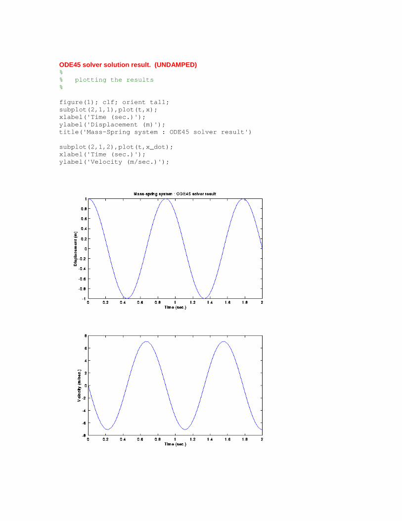
ODE45 solver solution result. (UNDAMPED) % % plotting the results % figure(1); clf; orient tall; subplot(2,1,1),plot(t,x); xlabel('Time (sec.)'); ylabel('Displacement (m)'); title('Mass-Spring system : ODE45 solver result') subplot(2,1,2),plot(t,x_dot); xlabel('Time (sec.)'); ylabel('Velocity (m/sec.)');

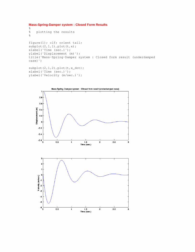
Mass-Spring-Damper system : Closed Form Results % % plotting the results % figure(1); clf; orient tall; subplot(2,1,1),plot(t,x); xlabel('Time (sec.)'); ylabel('Displacement (m)'); title('Mass-Spring-Damper system : Closed form result (underdamped case)') subplot(2,1,2),plot(t,x_dot); xlabel('Time (sec.)'); ylabel('Velocity (m/sec.)');

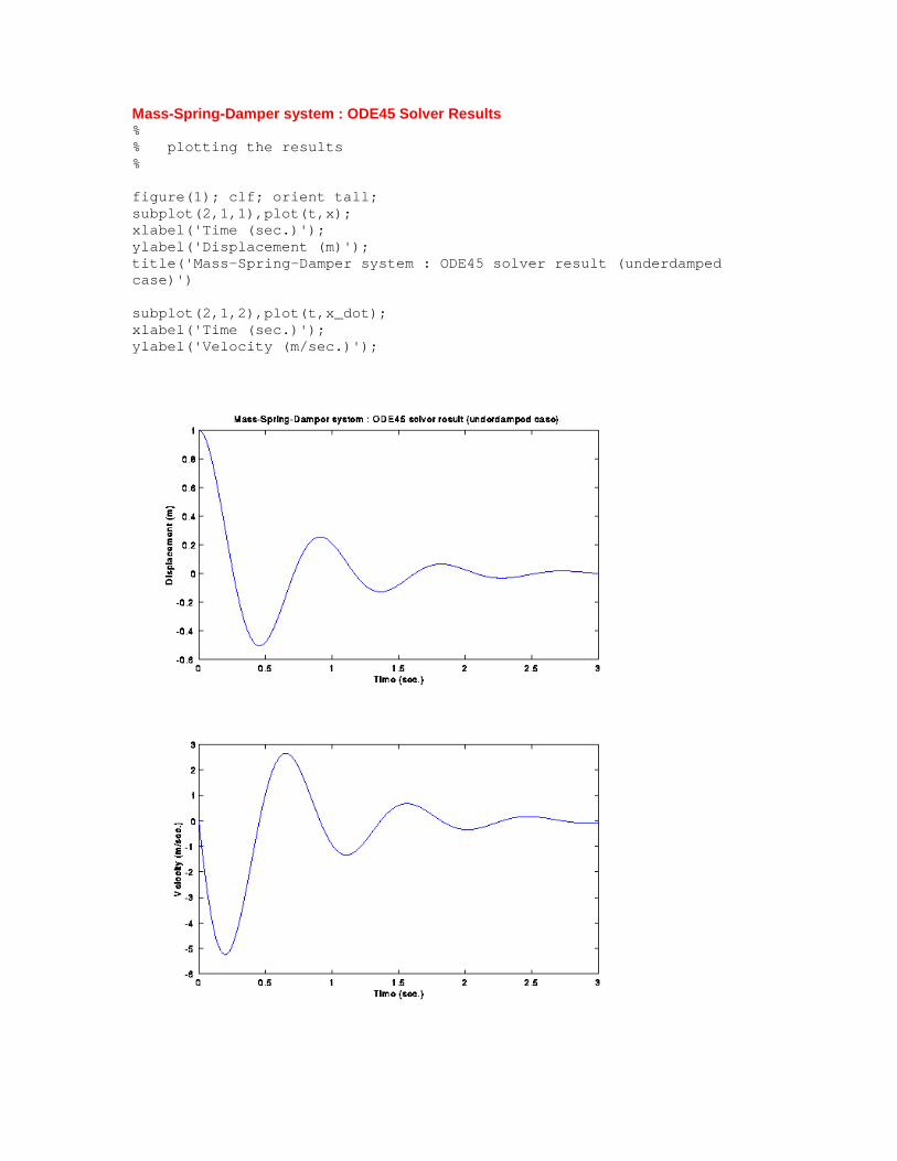
Mass-Spring-Damper system : ODE45 Solver Results % % plotting the results % figure(1); clf; orient tall; subplot(2,1,1),plot(t,x); xlabel('Time (sec.)'); ylabel('Displacement (m)'); title('Mass-Spring-Damper system : ODE45 solver result (underdamped case)') subplot(2,1,2),plot(t,x_dot); xlabel('Time (sec.)'); ylabel('Velocity (m/sec.)');