61aS,0SA,amO - Federation of American Scientists NM 87544 Phone: (505)667-4448 E-mail:...

,. ..,,, . . . ..-

..... . ,. ,,. - :*.6- .- ,- .. .,4.

- . .* . . . .. ..,, ,,.7.,..

~:.

. . . ,, ,, L

.

.

‘~6~~1a~~S,0SA,amOLosAlamos NationalLaboratory

AnMtlrnsatlvaActJorr/EqrratoPfXXtlldtyEntpbyas

Thisworkwassupportedby theUSDepartmentof Energy,Offke of BasicEnergySciences.

PreparedbyVickieMontoya,GroupT-4

DISCLAIMER

Tlsiareportwaspreparedasanaccountof worksponsoredbyanqmscyof theUnitedStxtesCoverrsrnent.Neitherthe UnitedStat= Govermnentnoranyagencythereof,rIJranyof theiremployees,makaanywarranty,expressor implied,orassumesanylegalliabilityor responsibilityfortheaccuracy,mmpletenesa,or usefuhreasof anyinformation,apparatus,product,or processdisclosed,or representsthat itausewotddnotinfringe@ately ownedrights. Referencehereinto anyspecitlccommercialproduct,process,orserviceby tradename,rrademark,marrufacturer,orothenviae,doesnotnecsarif y cmaatituteor implyMaendorsement,recommendation,or favoringbythe UnitedStata Governmentor anyagencythereof. ThetiewaandopinioNof authorsexpreswdhereiardonotneuxarifystateor reflectthoseof theUnitedStatesCawrrsnentoranyagencythereof.

LA-10244-M

UC-32 and 34Issued: September 1984

User%Manual for GRIZZLY

Joseph Abdallah, Jr.

.— ~-.

n

Los

—.-

.—

..s. - — .-— -. -

&— . .

.. . . ~ . .- ., .-. , ---. .

k.? —: .:

. .

. . . . —.-.,

,.= -.,.- ,., ,

., -: ..

.

AhmlosLosAlamos NationalLaboratoryLosAlamos,New Mexico 87545

ABOUT THIS REPORT

This official electronic version was created by scanning the best available paper or microfiche copy of the original report at a 300 dpi resolution. Original color illustrations appear as black and white images. For additional information or comments, contact: Library Without Walls Project Los Alamos National Laboratory Research Library Los Alamos, NM 87544 Phone: (505)667-4448 E-mail: [email protected]

USER’S MANUALFOR GRIZZLY

by

Joseph Abdallah, Jr.

ABSTRACT

This manual describes the first release of GRIZZLY, acomputer program to construct tables of atomic data for usein applications programs. The first release of GRIZZLY has thecapability to generate baseline equation-of-state tables forelements and mixtures using various physical models. GRIZZLYruns on the Los Alamos CRAY-1 computers.

I. INTRODUCTION

In the past it was usually necessary to run more than one code to calculate

a total equation-of-state (EOS) table. Hence, such a calculation was often

cumbersome and time consuming because of decentralization and data interfacing.

It has become apparent that development of an automated and centralized computer

program would improve the thoughput for producing EOS tables. The purpose of

GRIZZLY is to provide such a capability. EOS tables are collected and incor-1-3porated into the SESAMEdata library which can be accessed by several code

4-6packages which are used in various hydrodynamics programs (for example, Ref.

7). The physical models used in the first release of GRIZZLY are not intended to

be the latest in EOS theory, but they do represent computationally dependable

models that may be used to generate a baseline EOS. Future releases of GRIZZLY

will provide more sophisticated models capable of producing a higher quality

EOS. In the meantime, tables calculated by newer models may be read into GRIZZLY

for use if desired. Future plans for GRIZZLY also include the development of a

data base of material properties. Also planned is the computation of transport

properties such as opacity and conductivity.

GRIZZLY allows the users to

1. calculate contributions to the EOS based on physical models and to

produce tables;

2. perform table operations, i.e., combining tables, energy shifting,

density scaling, etc.;

3. mix tables using various schemes;

4. specify data to be used in calculating tables;

5. display input data and calculated tables in various formats;

6. read (write) tables from (to) files; and

7. execute procedures which are combinations of 1-6.

Items 1 through 7 are initiated via user supplied comands. These commands

may be read in from a input command file or entered directly from the users

terminal. Hence, GRIZZLY can be operated in both the production and interactive

modes. GRIZZLY is a table oriented code from which many commands either generate

tables or perform operations on tables. Table I-1 is an alphabetized list of

GRIZZLY commands. Each entry provides a brief description of the command and a

page number in this document where more detailed information may be found.

GRIZZLY consists of subpackages which evaluate the various models. These

subpackages are called by a common driver program with a common input base. Most

of the subroutines which evaluate models have been scavenged from existing

programs. The cold curve and nuclear models used by GRIZZLY have been extracted

from EOSCRAY8 and PANDA.9 The Thomas-Fermi-Dirac (TFD) model for electronic

excitations has been extracted from CANDIDE.10 The ideal mixture scheme has been

taken from MIXB.11Models can be evaluated either individually or as part of

multifunction procedures. Models are evaluated and tabulated on default or user

supplied compression and temperature grids. Two temperature equation-of-state

tables12 are easily obtained because models are tabulated individually.

All the data used by GRIZZLY are assigned default values. These values are

modified by issuing data specification commands. We plan to have default values

based on material when the data base becomes available.

Every attempt has been made to keep GRIZZLY easy to use in order to appeal

to various users. Even the occasional user should be able to generate a baseline

EOS with relative ease.

Generated EOS tables may be written to SESAMEfiles for use in programs

using such data. Tables may also be read and written in GRIZZLY data base

2

formatted files. All displays of tables or thermodynamic functions are written

to files which may be read by CURVES13 to provide a graphics interface.

Not all of GRIZZLY has been adapted from other codes. In fact, the portions

of GRIZZLY which are associated with items 2 through 7 represent new code devel-

opment.

Table I-2 describes the units used by GRIZZLY. Note that the compression

variable used in GRIZZLY is defined as

L,up=o

where p. is given by rhoref (Table I-1) and p is the mass density.

Section II discusses the general details of running GRIZZLY. Sections 111

and IV describe the procedures for calculating the EOS for elements and mixtures,

respectively. Sections V, VI, and VII discuss the models used for cold curve,

nuclear, and electronic table generation, respectively. Section VIII describes

the data specification commands. Section IX describes the compression and

temperature grids and the commands which control them. Section X describes the

various grid suppression strings. Section XI describes mixing schemes, these

include additive volume, partial pressure, and ideal mix algorithms. Section

XII describes the various table operations which are available under GRIZZLY.

Section XIII describes commands for displaying values of data used in EOS

generation. Section XIV discusses commands to display EOS tables and commands

to calculate and display thermodynamic properties along hugoniots, isobars,

isentropes, isotherms, and isochores. Section XV describes commands for EOS

table input and output. Section XVI presents several examples of running

GRIZZLY.

II. GENERALDETAILS

A. Running GRIZZLY

The executable binary file GRIZ and its associated data file GRZDBmay be

obtained from the common file system by using the command

MASS GET DIR=/LTE GRIZ GRZDB .

GRIZZLY may be executed using the CTSS execute line

GRIZ I = iname, P = pname, E = ename / t p.

3

The name of the input command file is specified by iname. The default for

iname is I. If iname equals TTY (teletype), commands are entered interactively.

If iname does not exist in the users local file space, control is transferred to

the terminal for interactive input. If the command file does not have an END

command, control is transferred to the TTY after

command file have been processed. This allows the

after performing a routine setup.

The name of the output print file is pname.

All the printed output is routed to pname.

all the commands from the

user to run interactively

The default for pname is P.

The name for the echo file is ename. The echo file contains all commands

entered during a session. If ename is not specified or ename = E, then commands

are echoed back to the TTY.

B. CommandFile Format

All GRIZZLY commands have the format

Cname PI Pz P3 ““” /.

The symbol cname is the alphanumeric command name, and the p. are associated1parameters delimited by blanks. The pi may be numeric or alphanumeric depending

on the command. A command parameter may be defaulted by entering an asterisk (*)

for that parameter or by ending the command prematurely. A single command may

extend over several lines. Each command must end with at least one blank and a

slash (/).

A command file is a collection of such commands on a file.

command must start on a new line. For example,

enamel PI P2 P3

P4 I

cname2 pl /

Each new

Most of this manual will be concerned with describing the commands which

are available under GRIZZLY.

c. Table Numbers—Grizzly currently has storage area allocated for seven 12,000 word tables.

Each storage area is identified by a table number i (1 : i : 7). Table numbers

are used as parameters on many commands.

4

D. EOS Evaluation

In general, the EOS of a material is calculated by combining three terms

P(p,T) = Pc(p) + Pn(p,T) + Pe(p,T)

E(p,T) = Ec(p) + En(p,T) + Ee(p,T)

A(p,T) = Ac(p) + An(p,T) + Ae(p,T) ,

where P is the pressure, E is the energy density, A is the Helmholtz free energy

density, p is the mass density, T is the temperature,theSubscriptc stands for

cold curve, n for nuclear, and e for thermal electronic excitations.

III. EOS FOR ELEMENTS

Tables for elements may be generated using the EOS command. This command

initiates a procedure which generates a separate cold curve table, nuclear

table, and electronic table [see Eq. (l)] and combines them to form a total

table. Default models are provided. The user may select different models by

issuing commands prior to the EOS command. The MODCcommand is used to select a

cold curve model, MODNto select a nuclear model , and MODEto select an elec-

tronic model. These commands are discussed in Sec. VIII. In addition, all data

must be set to desired values before the execution of the EOS command. The data

setting commands are discussed in Sec. VIII. The data requirements are included

in Sees. V, VI, and VII with the description of each model. The energy zero is

adjusted to correspond to zero pressure and to the reference temperature tref.

The EOS command format is

EOS ic in ie it / ,

where i is the cold curve table number, ic

is the nuclear table number, i e then

electronic table number, and it

is the total EOS table number. After execution

of the EOS command, the tables designated by ic, in, ie, and it should contain

the calculated values. A table may be used as input to EOS by specifying TAB

with the MODC, MODN, or MODEcommands (see Sec. VIII). This is convenient

because it avoids unnecessary recomputation of a table on successive executions

of the EOS command. The calculation of a particular contribution may be avoided

completely by specifying NONEwith the MODC, MODN, or MODEcommands.

5

Tables are generated on the compression and temperature grid existing when

EOS is executed (see Sec. IX) subject to suppression strings (Sec. X).

EOS can be used in a somewhat crude way for generating EOS tables for

mixtures. To use this method, the user enters atomic numbers and masses corre-

sponding to average values for the mixture.

Iv. EOS FOR MIXTURES

Tables for mixtures may be generated using the EOSMXcommand. The command

initiates a procedure which generates a separate cold curve table, nuclear

table, electronic table, and total EOS table. Default models are provided. The

user may select different models by issuing MODC, MODN,and MODEcommands prior

to the EOSMXcommand. These commands are discussed in Sec. VIII. All data must

be set to desired values before issuing the EOSMXcommand. In particular, the

MXTUREcommand must be issued to define the mixture composition. The MXTURE

command will set the atomic number, weight, reference density, and number of

mixture components, (NMIX). MXTLJREis discussed in Sec. VIII. The energy zero is

adjusted to correspond to zero pressure and to the reference temperature tref.

The command format is

EOSMXi/ .

On completion, table i contains the cold curve, table i + 1 contains the nuclear

contribution, table i + 2 contains the electronic contribution , and table i + 3

contains the total EOS; at least NMIX + 2 table storage areas are required to

execute EOSMX, hence i + NMIX + 1 < 7, or NMIX < 6 - i.— —

The cold curve calculated by EOSMXis that specified by MODCwith a high

density match to the mixed TFD cold curve. The mixed TFD cold curve is obtained

by generating the TFD cold curve for each component and then applying the ad-

ditive volume mixture rule. The nuclear table calculated is that specified by

MODNfor the average atom. The mixed electronic table is obtained by calculating

the thermal electronic table for each component and then applying the additive

volume mixing rule.

All tables are generated on the compression and temperature grids existing

when EOSMXis executed (Sec. IX) subject to suppression strings (Sec. X).

6

v. COLDCURVEMODELS

The cold curve described here corresponds to the electronic contribution to

the zero degree Kelvin isotherm. Contributions to the zero degree Kelvin iso-

therm due to zero point lattice vibrations are included in the nuclear model. In

addition to the commands and options discussed in this section, there are

specialized commands such as COLDMX,LJMATCH, MATCH, MATCH2, MXC, PCTAB, and

TFDCMXwhich may aid the user in constructing a cold curve. These are discussed

in Sec. XI.B and XII.B. All models may be calculated directly by using the

commands discussed below or through the EOS and EOSMXcommands. All models

discussed in this section need specification of zbar, abar, and rhoref (see

Table I-1) in addition to the specified data requirements.

A. TFD

A Thomas-Fermi-Dirac cold curve may be generated by using the command

TFDC i/ ,

where i is the table number associated with the calculated cold curve. Upon

completion of TFDC, table i will contain the TFD cold curve. The TFD cold curve

may be used in the EOS and EOSMXprocedure by setting mode (Table 1-1) equal to

TFD. The TFD cold curve is accurate at very high densities. The TFD calculations

are described

xalpha (Table

B. CHUG

The CHUG

in Appendix A. The only data

I-l).

cold curves consist of three

requirement is the exchange parameter

models joined smoothly to each other.

At compressions less than clj (see Table I-1) the. Lennard-Jones match formulag

is used. At intermediate compressions, the cold curve is chosen to reproduce9,14experimental shock data. The shock data is given in terms of a quadratic fit

to the shock velocity-particle velocity (us-up) curve. At compressions greater

than cmat (Table I-l), the high density match formula [see Appendix B] is used

to connect the cold curve to TFD. The method used in the intermediate compres-

sion region is discussed in9adapted from PANDA.

The CHUGcold curve may

C~Gimnlmn2/ ,

where i is the output table

detail in ReE. 14. The coding for CHUGhas been

be generated using

number, and mnl and mnq specify the nuclear model.1 &

The parameters mnl and mn2 may be given any of the values possible for modn1and

modn2 (see Table 1-1 and Sec. VIII). In addition, if the user wishes to specify

7

a tabular nuclear model, then mnl may be set to TAB and mn2 to the nuclear table

number. The nuclear table must be loaded at the time of CHUGexecution. If mnl

and mn~ are not specified the default nuclear model is used. The CHUGcold curve

is obtained with the EOS and EOSMKcommands with the setting mode = CHUG. The

default value for mode is CHUG.

The parameters clj, faclj, ecoh, co, Sl, S2, cmat, and xalpha are required.

In addition, all parameters for the nuclear model must be set. The us-up shock

fit parameters (co, Sl, S2) are specified using the SHKFIT or SHKFITKScommand.

c. CHUGT

The CHUGTcold curve is the same as CHUGexcept that a table of us, uP

(USUP command) points is provided instead of the quadratic fit. Linear inter-

polation is used to obtain the shock velocity at a given particle velocity. This

option is convenient if the u -u curve for the material has a phase transitionSP

or some other complex structure which the user wishes to reproduce.

The command

C~GT i mnl mn2 /

generates the CHUGTcold curve. All parameters have the same meaning as in the

CHUGcommand (Sec. V.B). The tabulated us-up points are specified using the USUP

or USUPKScommand.

D. MODMRS1

MODMRS1is the first of four variations of the modified Morse 15potential

in GRIZZLY. The modified Morse parameters for MODMRS1are determined such that

(1) the cold pressure vanishes at a given density (rcold) , (2) the cold iso-

thermal bulk modulus equals a given value (bcold) at that density, and (3) the

pressure goes to the free electron limit and high densities. MODMRS1has been

adapted from EOSCRAY.8

The MODMRS1cold curve may be calculated using

MODMRS1i / ,

where i is the associated output table number, or by using the EOS or EOSMX

command with mode set equal to MODMRS1.

The parameters rcold and bcold are required for MODMRS1.

E. MODMRS2

The modified Morse parameters for MODMRS2are determined such that (1) the

pressure at reference density (rhoref) and reference temperature (tref) vanishes,

(2) the isothermal bulk modulus at reference density and reference temperature

equals a

limit at

The

given value (bref), and (3) the pressure

high densities.

MODMRS2cold curve may be calculated using

goes to the free electron

MODMRS2i null mn2 /

or by using the EOS or EOSMXcommands with mode set equal to MODMRS2.All

parameters on the MODMRS2command have same ❑eaning as discussed in Sec. V.B.

The values tref, bref, and nuclear model parameters are required by

MODMRS2.

F. MODMRS3

The modified Morse parameters for MODMRS3are determined such that (1) the

pressure at reference density (rhoref) and reference temperature (tref) vanishes,

(2) the isothermal bulk modulus at reference density and temperature equals a

given value (bref), and (3) that the cohesive energy (ecoh) is reproduced. In

addition, the high density match formula is used to

curve connects with TFD.

The MODMRS3cold curve ❑ay be calculated using

MODMRS3i mnl mn2 /

or by using the EOS or EOSMX

eters have the same meanings

The values tref, bref,

required by MODMRS3.

commands with mode set

insure that the MODMRS3cold

equal to MODMRS3.All param-

as discussed in Sec. V.B.

cmat, xalpha, and nuclear model parameters are

G. MODMRS4

The modified Morse parameters for MODMRS4are determined using the same

conditions as MODMRS2.In addition, the high density match formula is used to

insure that the MODMRS4cold curve connects with TFD.

The MODMRS4cold curve may be calculated using

MODMRS4i mnl mn2 /

or by using the EOS or EOSMXcommands with mode set equal to MODMRS4.All

eters have the same meaning as discussed in Sec. V.B.

The values tref, bref, cmat, xalpha, and nuclear model parameters

required by MODMRS4.

VI. NUCLEARMODELS

The models presented in this section

equation of state from nuclear motion. Note

calculate the contribution to

that solid zero-point lattice

param-

are

the

vibra-

9

tions are included in the tables generated by these models. All models may be

calculated directly via commands discussed below or through the EOS and EOSMX

commands. Models discussed in this section usually require specification of

zbar, abar, and rhoref (Table I-1) in addition to the specified data require-

ments. If the CHARTD, COWAN,DEBYE, DEBYEC, EINSTN, EINSTC, or GIKNUCmodels

(see below) are involved, then a solid phase is present and a Griineisen pa-

rameter is required. Hence, igrun, gamref, and debref are required. If igrun =

3, gamref and debref are not used. Also, in all commands discussed below, i

refers to the table number associated with the calculated table. All models are

calculated on the compression-temperature grid existing at the time of command

execution. The default nuclear model is CHARTDwith a virial match.

A. CHARTD

The coding for the CHARTDnuclear model 16 has been adapted from the EOSCRAY8

code. This model may be calculated using

CHARTDi /

or by setting modnl equal to CHARTDfor the EOS and EOSMXprocedures. In GRIZZLY

and EOSCRAY, the Debye integral is calculated and in Ref. 16 it is approximated.

B. COWAN

The COWANnuclear model was developed at Los Alamos about 1957 by

R. D. Cowan. The coding for this model has been adapted from the EOSCRAYcode. 8

This model ❑ay be calculated using

COWANi /

or by setting modnl equal to COWANfor the EOS and EOSMXprocedures.

c. DEBYE, DEBYEC, EINSTN, EINSTC, and GIKNUC

These nuclear models have been extracted from the PANDAcode.g DEBYEand

EINSTN compute the Debye and Einstein solid models respectively. DEBYECand

EINSTC are modified versions of DEBYEand EINSTC in which only a finite number

of terms are included in the sum over vibrational levels. GIKNUCis the solid-

gas interpolation formula. These models are calculated using

DEBYEi /

DEBYECi/

EINSTN i /

EINSTC i /

GIKNUCi /

or by setting modn~ to the appropriate value for the EOS and EOSMXprocedures.

10

D. IDGAS

The ideal gas formula is evaluated using

IDGAS i /

or by setting modnl equal to IDGAS for the EOS and EOSMXprocedures.

E. VIRIAL

The virial match procedure has been extracted from PANDA.9 This match

procedure is used to provide a smooth interpolation between the solid and ideal

gas regions. A nuclear table with a virial match included may be generated by

using

VIRIAL i mn / ,

where mn may be CHARTD, COWAN,DEBYE, DEBYEC, EINSTN, EINSTC, or GIKNUC. If mn

is not specified, the default nuclear model is used. The virial match may be

used in conjunction with the EOS and EOSMXcommands by setting modn~ to VIRIAL

and setting modn2 to CHARTD, COWAN,DEBYE, DEBYEC, EINSTN, EINSTC, or GIKNUC.

The virial match requires a match compression (cvir) and a step size (dvir) for

taking a numerical derivative. See the comments in Ref. 9 concerning the restric-

tions for using the virial match.

VII. ELECTRONICMODEL

The only model currently available in GRIZZLY for calculating the contri-

bution to the equation of state from electronic excitations is the TFD method.

A. TFD

The coding for the TFD model has been adapted from a modified version of

the CANDIDEprogram. 10 This model is discussed in Appendix A. The commands

which evaluate the TFD model are

TFDC i /

TFDTOT i /

TFDTHMi / ,

where TFDC evaluates the cold curve (TFDC has already been discussed in Sec. V),

TFDTOT evaluates the TFD model, and TFDTHMcalculates the thermal contribution

to the EOS. The thermal table generated by TFDTHMis the TFDTOT table with the

cold curve subtracted. The thermal table is used for the electronic contribu-

tions in Eq. (l). The T_FDmodel is computed using the EOS and EOSMXcommands if

mode is set equal to TFD. When the EOS command is used, the TFD model is eval-

uated for the average atom. When the EOSMXcommand is used, the TFD model is

11

evaluated for each constituent atom of the mixture. All tables are generated on

the compression-temperature grids existing at the time of command execution

subject to suppression strings. The only required data for the TFDC, TFDTOT, and

TFDTHMcommands are zbar, abar, rhoref, and xalpha. The parameter tstfd is used

for TFDTOTand TFDTHM.

VIII. DATA SPECIFICATION COMMANDS

This section describes the commands which are used to specify the data

required by the models discussed in Sees. III through VII. Initially> all data

are assigned default values. Data specification commands are used to modify

these values. These commands should be issued prior to the model computation

commands. The LIST command (Sec. XIII) may be used to view data settings.

A. Commands

ABAR abar /

The ABAR command is used to specify the gram atomic weight of an element or the

average gram atomic weight for a mixture. The default abar = O.

ATOMzbar /

The ATOM command is used to initialize GRIZZLY for calculating an element. The

current version just resets all data defaults and sets the atomic number (zbar)

(see example 6 in Sec. XVI). In future versions of GRIZZLY, the ATOMcommand

will be used to provide the ‘best” default values for the specified element by

accessing the data base. The default zbar = O.

BCOLDbcold /

The BCOLD command is used to specify the isothermal bulk modulus (Mbar) at

density rcold (see RCOLD command) along the cold curve. The default bcold = O.

BREFbref/

The BREF command is used to specify the isothermal bulk modulus (Mbar) at rhoref

and tref (see RHOREFand TREF commands). The default bref = O.

CLJ clj /

The CLJ command is used to specify the compression where the Lennard-Jones match

procedure is to be applied to the cold curve. The default clj = 1.

CMATcmat /

The CMATcommand is used to specify the compression where the high density match

formula is applied to the cold curve. The default cmat = 1.5

12

CVIR cvir /

The CVIR command is used to specify the compression where the virial match

procedure is applied to nuclear models. The default cvir = 1.0.

DEBREFdebref /

This command is used to specify the reference Debye temperature (eV) used in

nuclear models. The default debref = O.

DEBKELdebref /

This command is equivalent to DEBREFexcept that debref is specified in degrees

Kelvin.

DEBSHKC. c /

This command is used to calculate the Debye reference temperature (debref) from

the sound speed c0( cm/psec) and Poissons ratio a. If c. is not specified it is

taken from an existing value (see SHKFIT command) , and a is set to 1/3 if it is

not specified. For example, DEBSHK/ will compute debref from the current c.

and (J = 1/3; DEBSHK0.5 / will compute debref using c. = 0.5, u = 1/3; DEBSHK

0.5 0.4 / will compute debref with c. = 0.5, and a = 0.4; and DEBSHK* 0.4 /

will compute debref with co

equal to the current value and ~ = 0.4. The entered

values of co

and o are not saved. The calculated value of debref is stored for

later use. The value of debref may be viewed by using the LIST / command.

DEBSHKKScoo/

This command is equivalent to DEBSHKexcept that c. is specified in km/see.

DVIR dvir /

This command is used to specify the spacing used to calculate numerical

derivatives for the virial match. The spacing is expressed as a fraction of the

virial match density. The default value for dvir is .001.

ECOHecoh /

This command is used to specify the cohesive energy (Mbar*cm3/g). The default

value for ecoh is O.

ECOHKCecoh /

This command is equivalent to ECOHexcept that ecoh is specified in kcal/mole.

EPSMIX epsmix /

This command is used to specify the accuracy criteria for additive volume mixing.-6

The default value for epsmix is 10 .

FACLJ faclj /

13

This command is used to specify the exponent used in the Lennard-Jones match

formula. The default value for faclj is 1.

GAMREFgamref /

This command is used to specify the reference Griineisen parameter. The default

value for gamref is O.

GAMSHKS1 ft /

This command uses the formulas of Ref. 9 to calculate the reference Griineisen

parameter from the slope of the us-u curve S1 and parameter ft. If S1 is notP

specified, the current value is used (see SHKFIT command). If ft is not speci-

fied, O is used. This command is similar to DEBSHK.

IGRUNigrun /

This command is used to specify the method for calculating the Griineisen param-

eter as a function of density. The following table describes the possible values

of igrun.

igrun type

1

2

3

4

5

6

Note that

Chart-D8’16

SESAME9

Cowan8

pr = constant

Pl/3r = constant

r = constant

the igrun = 3 option does not require specification of gamref and

debref. The default value for igrun is 3.

MODCmode /

This command is used to specify the cold curve model. Possible values for mode

are CHUG, CHUGT, MODMRS1,MODMRS2,MODMRS3,MODMRS4,and TFD (See Sec. V). In

addition, for the EOS command only , mode may be set to TAB if the user wishes to

supply a cold curve table, or mode may be set to NONEto neglect the cold curve

contribution. The default value for mode is CHUG.

MODNmodnl modn2 /

This command is used to specify the nuclear model. Possible values for the modnl

and modn2 combination are given in the following table.

14

modn1 modn

2

COWAN

CHARTD

DEBYE

DEBYEC

GIKNUC

EINSTN

EINSTC

IDGAS

VIRIAL COWAN

VIRIAL CHARTD

VIRIAL DEBYE

VIRIAL DEBYEC

VIRIAL GIKNUC

VIRIAL EINSTN

VIRIAL EINSTC

In addition, for the EOS commands

wishes to supply a nuclear table,

nuclear model. The default values

respectively.

MODEmode /

only, modnl may

or modn~ may be

be set to TAB if the user

set to NONE to omit the

for modnl and modn2 are VIRIAL and CHARTD,

This command is used to specify the electronic model. The possible value for

mode is TFD. In addition, for the EOS command only , mode may be set to TAB if

the user wishes to supply a thermal electronic table or mode may be set to NONE

to neglect the electronic contribution. The default value for mode is TFD. ‘

‘Tmnwxl ‘lal ‘lx2z2a2 ‘2 ““” ‘This command is used to specify a mixture. The parameter nw may be set to N if

input is in number fractions or to W if input is in weight fractions. The

parameters xi, z., a., and r. are the fraction, atomic number, atomic weight,1 1 1

and solid density for mixture component i. The parameters zbar, abar, rhoref,

and a set of tables describing the mixture are saved for further use upon

completion of MXTURE.These tables may be viewed using the LIST command.

RCOLDrcold /

15

The RCOLD command is used to specify the zero pressure density for the cold

curve. The default rcold equals O.

RHOREFrhoref /

The RHOREFcommand is used to specify the reference density at temperature tref

(see TREF command). The default value for rhoref is O.

S~ITCoS1 S2 /

This command is used to specify the fit to the u -u curve for a material. TheSP

fit formula is given by

u 2=s c. + ‘I”p + ‘2”p “

Since u and us

are required in units of cm/psec, c. has the units of cm/psec,P

‘1is dimensionless, and s z has units of psec/cm. The default values for these

parameters are c. = 51 = 52 = O.

s~ITKs C. S1 S2/

This command is equivalent to SHKYIT except that fit parameters are specified in

km/see units.

TREF tref /

This command is used to specify the reference temperature (eV). The default

value for tref is room temperature or 0.025692 eV.

TREFKELtref /

This command is equivalent to TREF except that tref is specified in degrees

Kelvin.

TSTFD tstfd /

This command is used to specify the temperature (eV) below which the TFD

energies are substituted by 1/2 TS, where T is the temperature, S is the

entropy, and T ~ tstfd. The substitution is used to eliminate noisy energy

results at low temperatures. The substitution is exact at high densities and

approximate at low densities. If tstfd is O, a default is chosen based on

atomic number. The default value for tstfd is O.

USEALL i /

This command is a combination of USEZ, USEC,

USEZ i /

This command is used to load the values of

values stored in table i.

16

and USET (see Sec. IX).

zbar, abar, and rhoref from the

usuP

This

used

u‘Pl s~

u‘p2 S2 “- ./

command is used to specify a tabulated us-u curve. Linear interpolation isP

to calculate shock velocities between table points. The maximum number of

u -u points allowed is twenty. All pairs ❑ust be specified in order of in-SP

creasing u . No shock table exists until a USUP command is executed. AllP

velocities are given in units of cm/psec.

USUPKSU U uPI s~

UP2 S2 . . . /

This command is equivalent to USUP except that velocities are entered in km/see.

XALPHAxalpha /

This command is used to specify the exchange parameter for the TFD model. The

default value for xalpha is 2/3.

ZBAR zbar /

This command is used to specify the average atomic number. The default value for

zbar is O.

IX. COMPRESSIONAND TEMPERATUREGRIDS

A. General

The models in GRIZZLY are calculated at the mass density and temperature

points specified by the compression and temperature grids existing at the time

of command execution. The mesh at which a given model is calculated is also

subject to the appropriate suppression string (see Sec. X). The density points

are obtained by multiplying the compressions by the parameter rhoref. Initially

default compression and temperature grids are read from the GRZDBfile. These

are general purpose grids which should be suitable for most applications. Hence,

the cumbersome task of specifying a grid is eliminated. The default compression

grid is presented in Table IX-1, and the default temperature grid is presented

in Table IX-2. Commands are also provided so the user may construct

meshes. These commands are described in Sec. IX.B. The LIST command

to view the existing compression and temperature grids.

B. Grid Manipulation Commands

alternative

may be used

In this section all commands starting with the letter C are associated with

the compression grid , and all commands starting with the letter T are associated

with the temperature grid.

17

TSUP k tl t; L2 t; . . . /

These commands construct grids based on suppressing portions of the default grid

(see Tables IX-1 and IX-2). The parameter k is a sparsing factor, for example,

if k equals 1 all default grid points are used, if k equals 2 every other grid

point is used, etc. The parameters f’li, q;, ti, t; specify ranges of values in

compression and temperature space, respectively, to be suppressed.

CGRI)ql r12 ““” /

‘Gm ‘1 ‘2 ‘“” /

These commands allow the user to specify the grid points directly. The t’I. are1compression points and the ti are temperature points. The points must be spec-

ified in ascending order.

CLIN n t’ll rln /

TLIN n t-l tn /

These commands allow the user to construct grids based on a linear spacing of

points. The parameter n is the number of points, rll and tln are the compression

limits, and t, and t- are the temperature limits.

CLOGn nl nn j

TLOG n tl tn /

These commands

of points. The

J.i

allow the user to construct grids based on a logarithmic spacing

parameters n, ql fln$ tl, and tn have the same meaning as in the

CLIN and TLIN commands.

CGRDArll ~2 ““” /

‘GmA ‘1 ‘2 “-. ‘These commands allow the user to add the specified points to the current grid.

The qi are the compression values and the ti are the temperature values to be

added to the grid.

CLINA n ql qn /

TLINA n tl tn /

These commands allow the user to add a linearly spaced set of points to the

current grid. The parameter n is the number of points to be added and fll, t’ln,

‘1’and t n specify the compression and temperature limits, respectively.

CLOGAn ql tln /

TLOGAn tl tn /

These commands have the same meaning as CLINA and TLINA except that the points

have logarithmic spacing.

18

USEC i /

USET i /

These commands are used to specify the grids from existing tables. USEC sets the

compression grid from table i, and USET sets the temperature grid from table i.

x. SUPPRESSION

A. General

Some of the physical models used by GRIZZLY do not work over the wide range

of compressions and temperatures which need to be considered. Grid suppression

is used to eliminate trouble regions for a particular model prior to calculation.

Allowance is also made for sparsing the grids for a particular model. For each

model or group of models there

read from the GRZDB file. Each

and temperatures. Each string

values to be suppressed. These

commands (see below). The grid

exists a suppression string which is initially

string controls the suppression of compressions

contains sparsing factors and ranges of grid

values may be altered by issuing the appropriate

for a particular model is determined by applying

the sparsing factor and suppression ranges to the current grid (see Sec. IX).

Suppression strings may be viewed by using the LIST command (see Sec. XIII). The

commands which control suppression strings are discussed in Sec. X.B.; suppres-

sion of data in existing tables is discussed in Sec. X.C.

B. Suppression Control Commands

This section describes the commands which allow the user to alter the

suppression strings. There are four groups of models for which suppression

strings exist. All the cold curve models are subject to a single compression

suppression string (COLD). All the nuclear models are subject to a single sup-

pression string (NUC). All mixing models are subject to a single suppression

string (MIX). The TFD model is subject to its own suppression string (TFD). The

sparsing factors k are defined such that k = 1 indicates no sparsing, k = 2

means every second point is used, k = j means every jth point is used.

KCOLDk /

KCMIX k /

KCNUCk /

KCTFDk /

These commands

for cold curve

control

models,

the sparsing of compressions. KCCOLDcontrols sparsing

KCMIX controls the sparsing for mixture models, KCNUC

19

controls the sparsing for nuclear models, and KCTFD controls sparsing for the

TFD model. The parameter k is the sparsing factor. The default value is 1 for

all compression sparsing factors.

KTMIX k /

KTNUCk /

KTTFD k /

These commands control the sparsing of

sparsing for mixture, nuclear, and TFD

the sparsing factor. The default value

SCMIX ql ~; t12

‘Cwc q~ q; q~

SCTFD ql qi f12

These commands

SCCOLD, SCMIX,

r-l; /r-l; /r-l; /control the parameters

temperatures. KTMIX, KTNUC, KTTFD control

models, respectively. The parameter k is

is 1 for all temperature sparsing factors.

associated with compression suppression.

SCNUC, and SCTFD control suppression for cold curve, mixture,

nuclear, and TFD models, respectively. The parameters q. and q~ (i = 1,2) define1

lower and upper limits, respectively, for suppression region i. The default-lovalues for all models are tll = -1, ~; = 10 , Q2 = -1, and q; = -1. An asterisk

(*) should be entered in any field for which the user wishes the associated

value to remain unchanged.

STMIX tl ti t2 t; /

STNUCt t’ t1 1 2t;’STTFD tl ti t2 t; /

These commands control the parameters associated with temperature suppression.

STMIX, STNLJC,and STTFD control suppression for mixture, nuclear, and TFD models,

respectively. The parameters t. and t ~ (i =1,2) define lower and upper limits,1

respectively, for suppression region i. The default value for all ti and t; is

-1, except for the TFD model where tl = 10-4

and t’1 = 0.2499. An asterisk (*)

should be entered in any field for which the user wishes the associated value to

remain unchanged.

c. Table Suppression

The user may sparse and suppress points of an existing E(IS to remove

data or for other reasons. This operation is performed by the SUP command.

command has the format

SUP il i2 / .

bad

This

20

The SUP command suppresses data on table il and creates the resultant (sup-

pressed) table i2. Suppression conditions are imposed by issuing the following

commands prior to SUP execution. Note that this type of suppression is based on

mass density and not compression.

KRTABk /

KTTAB k /

These commands are used to specify the density and temperature sparsing factors

respectively, for table suppression. The default value for k is 1.

SRTAB rl r; r2 r; /

STTAB tl t; t2 t; /

These commands are used to specify the density and temperature suppression

regions, respectively, for table suppression. The ri and r; define lower and

upper bounds, respectively, for density suppression in region i. The ti and t;

define lower and upper temperature bounds, respectively, for region i. The

default value for all r., r!1 1’

ti, and t: is -1 (no suppression). An asterisk (*)

should be entered in any field for which the user wishes the associated value to

remain unchanged.

XI. MIXTURES

A. General

The additive volume, ideal, and partial pressure mixing

available in GRIZZLY. These schemes are discussed in Appendix

schemes are

C. All three

schemes may be used in commands where the user specifies the constituent tables.

The additive volume procedure is used when mixing involves specified mixtures

(see MXTUREcommand). Sec. XI.B. discusses the commands associated with table

mixing, and Sec. XI.C discusses utility commands available for specified mix-

tures.

B. Table Mixing Commands

‘WIX ‘w ‘1 ‘1 ‘2 ‘2 ““” i/

IDMIX nw il xl i2 x2 . . . i /

‘PMIX ‘w ‘1 ‘1 ‘2 ‘2 ““” i/

These commands apply the corresponding mixing schemes to the specified

tables and create a mixed EOS table. The commands AVMIX, IDMIX, and PPMIX apply

the additive volume, ideal, and partial pressure mixing schemes, respectively.

The parameter nw can be set to N if number fractions are input or to W if weight

21

fractions are input. The ij’s are table numbers for mixture component j, and the

‘s are number or weight fractions depending on the value of nw. The parameter‘ji specifies the output “mixed” table number. All tables ij must be loaded prior

to command execution. Note that table numbers and fractions are not saved for

further use.

c. Specified Mixtures

A specified mixture is defined using the MXTUREcommand (see Sec. VIII). In

addition to the EOSMXcommand (see Sec. IV), several other miscellaneous commands

which operate on specified mixtures

in this section. The definition of

using the LIST command. In all the

of mixture components.

COLDMXi mc mnl mn2 /

This command generates a mixed cold

are available. These commands are presented

the current specified mixture may be viewed

command discussed below, NMIX is the number

curve using the method described in Sec. IV.

The parameter i specifies the “mixed” cold curve table number. This command uses

NMIX + 1 table areas starting at table i; hence, table i through i + NMIX are

used and any data in these tables will be overstored upon completion of COLDMX.

The parameters mc, mnl, and mn2 may optionally be used to specify the cold curve

and nuclear models. If these parameters are not specified, the default models

are used.

ELECMXi me /

This command calculates a mixed thermal electronic table using the method de-

scribed in Sec. IV. The parameter i specifies the ‘mixedN table number. The

command requires NMIX + 1 table areas starting at table i; hence, table i through

i + ~IX are used and any data in these tables will be overstored upon completion

of ELECMX. The parameter me may optionally be used to specify the electronic

model; if it is not specified, the default model is used.

MXi/

MXC i /

These commands perform additive volume mixing of EOS tables and cold curve

tables, respectively. Tables i through i + NMIX - 1 are mixed, and the results

are stored into table i + NMIX. Table i is assumed to be loaded with data for

component 1, table i + 1 is assumed to be loaded with data for component 2, etc.

TFDCMXi /

TFDMXi /

22

These commands calculate TFD cold curves and TFD thermal electronic tables,

respective Iy, for each component of the specified mixture. The calculated table

for component 1 is stored on table i, the table for component 2 is stored in

table i + 1, etc.

XII. TABLE OPERATIONS

A. General

This section describes commands which perform useful operations on EOS

tables.

CHANGEi rtpea/

This command changes the pressure, internal

specified value (p, e, and a, respectively)

energy, and free energy to the

for the grid point

specified density r and temperature t of table i. An asterisk

entered for p, e, or a if the user does not want the associated

changed.

COPTABil i2 /

Copies table il to table i2.

RATil i2/

closest to

(’~) may be

values to be

This command creates table i2 by interpolating table il to the current compres-*-I

sion and temperature grids using the rational function method. l’

RSCALE i r /

This command scales table i to the specified reference density

density and high temperature regions of the EOS are preserved.

prescription is presented in Appendix D.

SCALEia/ .

r. The low

The scaling

This command scales table i to the specified atomic weight a. SCALE is useful

for generating equations-of-state for various isotopic compositions of a mate-

rial. This type of scaling is discussed in Ref. 4.

SHFTi es /

This command subtracts the specified energy shift (es) from internal energies

and free energies of table i.

‘Tm ‘1 ‘2 ‘This command computes the energy where the pressure vanishes at tref on table il

and subtracts this energy from both tables il and i2“

SUBCLDi /

23

This command subtracts the isotherm of lowest temperature of table i from all

isotherms of table i.

TOTAL ic in ie it /

This command combines a cold curve table i a nuclear table in, and anc’

electronic table i e to form a composite (total) EOS table it. The tables ic, in,

and i e must be loaded prior to execution of TOTAL. Any contribution may be

neglected by entering zero for ic, in, or ie.

B. Cold Curves

This section describes commands which perform table operations which are

useful for constructing cold curves.

LJMATCHil i2 mnl mn2 /

This command applies the LJMATCHformulag to cold curve table il and generates

table i2 at the current compression grid. The parameters mnl and mn2 specify the

nuclear model (see Sec. V.B.). The default model is used if mnl and mn2 are not

specified. LJMATCHuses the parameters clj, faclj, ecoh, and nuclear model

parameters.

MATCHil i2 i3 /

This command applies the high density match (Appendix B) to low density table il

and high density table i2 to form the composite table i3 at the current compres-

sion grid. The high density match is applied at compression cmat.

‘TCH2 ‘1 ‘2 ‘3 ‘nl ‘n2 /

This command applies the Lennard-Jones match formulag to cold curve table il and

the high density match (Appendix B) formula to il and i2 to form a composite

table i3. The parameters mnl and mn2 have the same meaning as in Sec. V.B. In

addition to nuclear parameters, clj, faclj, ecoh, and cmat are used.

PCTAB i r p1 1 rz P2 . . . . /This command constructs a cold curve table i from density (rj) and pressure (pj)

data. Energies are calculated by numerically integrating the pressure.

XIII. DATA DISPLAY

LIST item itp /

This command generates displays of the raw data used in constructing an

equation-of-state table. All values listed correspond to those existing at the

time the LIST command is executed. The parameter item specifies the type of data

to be listed. Possible values for item are DATA (default), TEMP, COMP, GRIDS,

24

MIX, SUP, and ALL. DATA will provide a list of raw data used by the models (see

Sec. VIII), TEMPwill display the temperature grid, COMPwill display the compres-

sion grid, GRIDS will display both the temperature and compression grids, MIX

will display information stored for specified mixtures, SUP will display sup-

pression strings, and ALL will display all of the above. The parameter itp

controls where the display is printed. If TTY is entered (default), the display

is written to the user’s terminal. Any other setting of itp will route the

display to the print file. Note that the commands

LIST /

LIST DATA /

LIST DATA TTY /

LIST * TTY /

LIST * /

LIST * * /

are all equivalent. Example 6 in Sec. XVI uses the LIST command to display

default data settings.

XIV. EOS DISPLAY

Commands are available in GRIZZLY for displaying EOS data from tables.

There are commands which display actual table points and commands which use

interpolation to display the EOS along hugoniots, isentropes (constant entropy),

isobars (constant pressure), isochores (constant density), and isotherms

(constant temperature). All displays can be sent to the user~s terminal, the

print file, or both. CURVES13may be used to generate graphical displays from

print files. Sections XIV.A., B., C., D., E., and F. discuss the commands

associated with displaying table points, hugoniots, isentropes, isobars,

isochores, and isotherms, respectively.

Displays produced by commands in this section can be presented in other

units provided that the conversion involves only simple multiplication. User

units are defined through the DUNITS command. Note that if alternative units are

defined then all commands in this section requiring data must be entered in user

units.

DUNITS run tun pun eun vun /

This command allows the user to modify display units. The parameters run, tun,

pun, eun, and vun are density, temperature, pressure, energy, and velocity

25

multipliers, respectively. All parameters correspond to conversion factors for

converting GRIZZLY units (Table I-2) to user units. All factors have a default

value of 1.

A. Table Points

DISPLAY i rl r2 tl t2 lab /

D t t lab /‘rlr2 1 2PRINT

i ‘1 ‘2 ‘1 ‘21ab’P

i ‘1 ‘2tl ‘21ab’These commands display the tabulated EOS values for table i. DISPLAY presents

the table at the users terminal , and PRINT routes the table to the print file. D

is shorthand for DISPLAY and P is shorthand for PRINT. The parameters r1

and r2

define a density window. The parameters tl and t2 define a temperature window.

Any points falling within both windows are displayed. The default values for rl,

‘2’ ‘1’ and t2 are -1.0, 1.0E300, -1.0, and 1.0E300, respectively. The parameter

label is an optional eight character alphanumeric the user may define to label

the display.

RHOiitp/

This command displays the density grid for table i. If the parameter itp is set

to P then the display is sent to the print file; otherwise, the display is

presented at the user’s terminal.

TEMPi itp /

This command displays the temperature grid for table i. If the parameter itp is

set to P then the display is sent ot the print file ; otherwise, the display is

presented at the user’s terminal.

B. Hugoniots

The HUG command is used to display EOS information for a material under-

going shock compression from some initial state. Solutions to the Rankine-Hugoniot

relation are displayed along a prescribed temperature mesh. The default

temperature mesh is 0.026, 0.05, 0.1, 0.15, 0.2, 0.25, 0.30, 0.35, 0.40, 0.45,

and 0.5 eV. Alternative temperature meshes ❑ay be constructed using the THGRD,

THLIN, and THLOG commands. The initial state of the material is taken to be a

compression of 1 and temperature of 0.025692 eV. The initial state may be altered

by issuing a

HUGi idev/

This command

26

HUGI command.

displays a hugoniot from table i. If the parameter idev is omitted

or set to TTY, the display is sent to the user’s terminal. If idev is set to P,

the display is sent to the print file. If idev is set to B, the display is sent

to both the terminal and print file.

CHGMchgm /

This command is

corresponding to

for solutions of

HUGI chgi thgi /

used to specify the maximum hugoniot compression. The density

this compression (chgm) is used as a upper limit when searching

shock relationships. The default value for chgm is 3.

This command is used to alter

The parameter chgi specifies

perature.

‘HGm ‘1 ‘2 ““” /

THLIN n tl tn /

THLOGn tl tn /

the initial state used for computing the hugoniot.

the initial compression and thgi the initial tem-

These commands are used to alter the hugoniot temperature mesh. THGRD, THLIN,

and THLOGare analogous to TGRD, TLIN, and TLOG (see Sec. IX), respectively. A

maximum of 50 temperatures is allowed.

c. Isentropes

The ISENT command is used to display EOS information along paths of constant

entropy. Isentropes are generated on a prescribed density mesh. The default

density mesh consists of 13 logarithmically spaced points between 10-3 3and 10 .

Alternative meshes may be constructed using the RENGRD, RENLIN, and RENLOG

commands.

ISENT i r t idev /

This command displays an isentrope from table i. The density r and temperature t

are used to determine the entropy for the isentrope. Table i must include the

free energy. The parameter idev is defined in Sec. XIV.B. (HUG command).

‘NGm ‘1 ‘2 ““” ‘RENLIN n rl rn /

RENLOGnrl rn/

These commands are used to alter the density mesh. RENGR.Dis used to specify

individual density points, RENLIN is used to specify a linear density mesh, and

RENLOGis used to specify a logarithmic density mesh. The parameter n specifies

the number of points, and r1

and r specify the lower and upper density limits,n

respectively. The maximum number of densities allowed is 50.

27

TENT tentl tent2 /

This command is used to alter the temperature search limits used in calculating

isentropes. The parameters tentl and tent2 specify the lower and upper limits,

respectively. The default values for tentl and tent2 are O and 100000 eV,

respectively.

D. Isobars

The ISOBAR command is used to display EOS information along paths of

constant pressure. Isobars are computed on a prescribed temperature mesh. The

default mesh is O, 0.025692, 0.1, 0.5, 1, 3, 10, 30, 100, 300, and 1000 eV. The

commands TISBGRD, TISBLIN, AND TISBLOG may be used to construct alternative

meshes.

ISOBAR i p idev /

This command displays an isobar from table i. The parameter p specifies the

pressure, and idev has been discussed in Sec. XIV.B.

RISOB risobl rosob2 /

This command is used to alter the density search limits. The parameters risobl

and risob 2are the lower and upper density search limits, respectively. The

default values for risobl and risob2 are the density limits of the table spec-

ified in the ISOBAR command. These parameters may be varied to avoid diffi-

culties caused by nonuniqueness in the vapor dome region.

TISBGRD tl t2 . . . /

TISBLIN n tl tn /

TISBLOG n tl tn /

These commands are used to alter the isobar temperature mesh. TISBGRD, TISBLIN,

and TISBLOG are analogous to TGRD, TLIN, and TLOG (see Sec. IX), respectively.

The maximum number of temperatures allowed is 50.

E. Isochores

The command ISOCHR is used to generate the EOS at constant density along a

mesh of temperatures. The default mesh is O, 0.025692, 0.1, 0.5, 1, 3, 10, 30,

100, 300, and 1000 eV. The temperature mesh may be altered by using the TISCGRD,

TISCLIN, or TISCLOG commands discussed below.

ISOCHR i r idev /

This command is used to display an isochore from table i. The parameter r spec-

ifies the isochore density. The parameter idev has been discussed in Sec. XIV.B.

(HUG command) .

28

‘lscGm ‘1 ‘2 “ “ “ ‘TISCLIN n tl tn /

TISCLOG n tl tn /

These commands are used to prescribe a temperature mesh for displaying isochores.

TISCGRD, TISCLIN, and TISCLOG are analogous to TGRD, TLIN, and TLOG. The maximum

number of temperatures is 50.

F. Isotherms

The command ISOTHMis used to generate the EOS at constant temperature

along a mesh of densities. The default mesh is 13 logarithmically spaced points

between 10-3and 103. The density mesh may be altered by using the RISTGRD,

RISTLIN, and RISTLOG commands discussed below.

ISOTHMi t idev /

This command is used to display isotherms from table i. The parameter t is the

isotherm temperature. The parameter idev has been discussed in Sec. XIV.B. (HUG

comand).

‘lsTGm ‘1 ‘2 “.. /

RISTLIN n rl rn /

RISTLOG n rl rn /

These commands are used to prescribe a density mesh for displaying isotherms.

RISTGRD, RISTLIN, and RISTLOG are analogous to RENGRD,RENLIN, and RENLOG(see

Sec. XIV.C.). The maximum number of densities allowed is 50.

xv. FILE INTERFACES

File interface commands allow the user to read and write EOS data to files

of various formats. EOS tables can be written to SESAMEfiles or GRIZZLY data

base files. SESAMEis currently the format supported by T-4 for storing EOS,

opacity, and conductivity data. The GRIZZLY data base files are compatible with

those being used for NLTE (Non-Local

SESAME files have the advantage

codes existing at the laboratory.

GRIZZLY data base files have the

Thermodynamic Equilibrium) work in T-4.

that they interface with many computer

advantage of a more flexible data identi-

fication scheme. Also, data records may be added to an existing file without

running an intermediate data base management program.

The commands discussed below control the reading and writing of EOS tables.

‘SES ‘d ‘n ‘1 ‘1 ‘2 ‘2 ... ‘

29

WSES id fn il tl i2 t2 . . . ipe /

These commands read and write SESAMEfiles, respectively. The parameter id is

the SESAMEmaterial number, fn is the SESAMEfile name, ik is the internal table

number, and tk is the SESAMEtable number. For RSES the SESAMEfile fn is read

and tables t of material id are read into internal table numbers ik k. For WSES a

SESAMEfile fn is created with one material of number id and SESAMEtable num-

bers tk corresponding to internal table numbers i k. These commands also perform

the units conversions which are required. If the parameter ipe is set to PE only

the pressure and internal energy tables are written; thus the Helmholtz free

energy is not included in the SESAMEtable.

RTAB i fn kyl ky2 . . . /

WTABi fn kyl ky2 . . . /

These commands are used to read and write data base files , respectively. The

parameter i is the table number, fn is the file name, and the kyk are a set of

to 3 numeric or hollerith identification keys. RTAB will read the data record

1

with identification keys kyk from file fn into GRIZZLY table i. WTABwill write

internal table i to file fn with keys kyk. If fn does not exist in the users

local file space, fn will be created. If fn does exist in the user’s space, then

the data will be added to file fn. If the identification keys are identifical to

ones existing on the file, the new data will replace the existing data.

XVI. EXAMPLES

1. Figure 16-1-1 shows a run of GRIZZLY to generate an aluminum EOS using the

default models. The atomic number, atomic mass, normal density, and cohesive

energy are specified by the first four commands. The SHKFIT command is used to

supply the u -u fit18 for the CHUGcold curve. The EOS command calculates the5P

equation of state. The cold curve is stored in table 1, the nuclear contri-

bution is stored in table 2, the electronic contribution is stored in table 3,

and the total EOS is stored in table 4. The WSES command is used to write these

tables to SESAMEfile S3716 with material number 3716. The code SES2D19was used

to access this file and generate the plots shown in Figs. 16-1-2 to 16-1-10.

Figures 16-1-2, 16-1-3, and 16-1-4 show the total pressure, total internal

energy, and total Helmholtz free energy, respectively. Figures 16-1-5, 16-1-6,

and 16-1-7 show the electronic contribution for the pressure, energy, and free

energy, respectively. Figures 16-1-8, 16-1-9, and 16-1-10 show the nuclear

30

contribution for the pressure, energy, and free energy, respectively. The

variables are plotted as a function of mass density for a given temperature.

2. Figure 16-2-1 shows a run of GRIZZLY which accesses the data generated in

example 1 and calculates the hugoniot. The generated hugoniot is compared with

experimental shock data in Fig. 16-2-2. Figure 16-2-2 was generated using

CURVES13 with the GRIZZLY output file, the experimental shock data were ex-

tracted from the HUGDATA20file.

3. Figure 16-3-1 shows a run of GRIZZLY to generate an EOS for silver. This

example is more detailed than example 1 because more parameters are specified.

The value for normal density, bulk modulus, Debye temperature, and cohesive

energy were taken from Ref. 21. Note the user specified compression grid and the

suppression of temperatures above 100 eV. The TSTFD command is used to eliminate

some wiggles in the TFD energies at 10 eV and below. A mod-Morse cold curve is

used with the solid-gas formula plus virial match nuclear model. Note the data

and grids are listed before the EOS is computed. After the EOS is calculated the

tables are written to a SESAMEfile and the principal hugoniot is sent to the

print file with user defined units. Figures 16-3-2 through 16-3-10 display the

calculated total, electronic, and nuclear EOS surfaces. Figures 16-3-11 and

16-3-12 compare the theoretical and experimental hugoniots.

4. Figure 16-4-1 presents the GRIZZLY run for beryllium oxide (BeO). The MXTURE

command is used to define the mixture components. The actual normal density is

supplied with the RHOREFcommand. The KCTFD command is used to sparse the TFD

tables to make the run faster. The CHUGTcold curve option is used to replicate18a complex hugoniot structure, and hence a USUP command is issued. The EOSMK

command is used to calculate the EOS. Note that suppression is used to get rid

of data above a compression of 1000. Most of these data are not good because of

applying the mixing scheme to densities beyond the validity of the constituent

tables. The tables are then written to a SESAMEfile and a hugoniot is cal-

culated. Figures 16-4-2 through 16-4-1o present the calculated EOS surfaces. The

wiggles in the electronic tables (16-4-5 through 16-4-7) at low temperatures are

caused by interpolation to temperatures not tabulated for each of the con-

stituent materials. These wiggles do not appear on the total EOS surface because

the electronic contribution is small in this region. Figures 16-4-11 shows a

comparison of the calculated hugoniot with experiment. The theoretical hugoniot

does not approach the sound speed (small particle velocities) because there are

31

not enough grid points around ambient conditions to resolve the structure of the

EOS.

5. Figure 16-5-1 shows an example of mixing pre-existing tables. The tables are

read from the SESAMElibrary and mixed with the various schemes. The mixture

corresponds to that of Appendix C. The print file generated by this example is

shown in Fig. 16-5-2.

6. Figure 16-6-1 shows an interactive run of GRIZZLY to exercise the LIST

command. Note the default values of the various parameters. Also note that a

MXTUREcommand is invoked as a prerequisite to exercising a LIST MIX / command.

The columns labeled WMIX, FMIX, ZMIX, AMIX, and RMIX correspond to weight frac-

tion, number fraction, atomic number, atomic weight, and normal density of each

component. Note that the MXTUREcommand also sets zbar, abar, and rhoref.

ACKNOWLEDGMENTS

The author is indebted to Bard Bennett, F. Dowell, Brad Holian, Kathy

Holian, Walter Huebner, J. D. Johnson, Al Merts, and Galen Straub for their

involvement with GRIZZLY. The author is also indebted to Jerry Kerley

PANDA, to David Liberman for providing Appendix A, and to Jean Trujillo

Vickie Montoya for typing the manuscript.

for

and

32

APPENDIXA

CANDIDE

CANDIDE is the computer program which

Thomas-Fermi-Dirac model to obtain equationA,. . .

uses a temperature dependent

of state data. Like other

Thomas-Fermi modelszz’zs it assumes an average atom. Unlike Ref. 23, it uses a

zero temperature expression for exchange at all temperatures. This has the

advantage of simplicity and also avoids the well known incorrect low temperature

behavior characteristic of the Hartree-Fock expression for exchange. At high

temperatures there is some error as a result of this approximation, but it is

small in comparison with the thermal contributions to the kinetic and potential

energies.

The model is based on an expression

E = K + U + V + W is the internal energy,

is the kinetic energy

u=- J dr # p(r)

is the electron-nucleus potential energy,

is the electron-electron potential energy,

for the free energy, F = E - TS, where

and

is the zero temperature

dr p(r)%(r)

expression for the exchange energy, and

(A-1)

(A-2)

(A-3)

(A-4)

33

s=- kB .fJ %# 2{f(r,p)log f(r,p) + [1 - f(r,p)]log[l-f(r,p)]] (A-5)

is the entropy. In these equations

P(r) = .( Q 2f(r,p)1?

(A-6)

is the density of electrons,

~(r)= [3n2p(r) ] 1/3 (A-7)

is the Fermi wave number, f(r,p) is the Fermi-Dirac distribution function, and

Xa is a parameter which normally is 2/3. All integrals on r are understood to

run from O to R--the radius of the atomic sphere --while integrals on p run over

all of momentum space.

The free energy, F, is to be minimized subject to the condition that the

number of electrons in the atomic sphere,

N = ~ dr p(r), (A-8)

is fixed. For neutral atoms N = Z. The minimization of F, subject to the

constraint that N is fixed, is accomplished by setting

6(F - pN)6F = O = ~ .s(r,p) - p + kBT log ~ ‘(r’p)

h3 - f(r,p) ‘

where

f + v(r)&(r,p) = Zm

and

Ze2v(r) =-=+~dr’ e2p(r’)lr- r’!

- # (~ Xa)~(r) .

(A-9)

(A-1O)

(A-n)

34

The solution of this is the Fermi-Dirac distribution function

f(r,p) = l/{exp[(&(r,p) - P)/kBT] + 1] .

23The potential v(r) + ~ ~ Xa ~(r) satisfies the Poisson equation

23-V2[v(r) + ~ (~ Xa)~(r)] = 47ce2[Z6(r) - p(r)] ,

(A-12)

(A-13)

and the electron

p(r) =~qh3

density is

2(A-14)

exp # + v(r) - p /kBT + 1

These last two equations are solved for v(r) and p(r) by CANDIDE. The chemical

potential is adjusted to make the number of electrons, N, correct. When p(r)

and v(r) are known, the thermodynamic functions, including the pressure, are

calculated.

35

APPENDIXB

HIGH DENSITY MATCH

The high density match formula in GRIZZLY is a modified version of the TFD9

match formula of PANDA. The major differences are (1) the GRIZZLY version has

one less parameter and therefore one less condition to satisfy, and (2) the

formula as implemented in GRIZZLY is not restricted to TFD.

The purpose of the high density match formula is to join smoothly a cold

curve valid at densities below a match density (pm) to a cold curve valid at

higher densities. The match density used in GRIZZLY is the product of rhoref and

cmat. For densities p < pm, the low density cold curve energies EL and pressure

PL are used. For densities p ~ pm, the cold curve is expressed as

EC(P) = [EH(P) - EH(pM)]y(p) + MC and (B-1)

Pc(p) = I?H(P)Y(P) + P2[EH(P)- EH(PM)] ~ ~ (B-1)

where E and P are the cold energies and pressures, respectively, EH and pH areL L

the high density cold energies and pressures, and Y is a interpolation function

given by

b b2Y(p) =1+++— 4/3 “

P

The constants AE bl,c’

EC(PM) = EL(pM)

‘c(pM) = ‘L(pM)

and

dP dPLc‘~ “dp PM

PM

and b2 are determined by requiring that

9

9

(B-3)

(B-4)

(B-5)

(B-6)

36

The version of the TFD match in PANDAhad an additional term in Eq. (B-3). In

order to evaluate a coefficient for this term , an extra condition involving the

second derivative of the pressure was imposed. This term is used in P~A to

insure the continuity of the second derivative of the pressure. This derivative

is used in methods which compute the Grtineisen parameter from the cold curve.

Since the current version of GRIZZLY has no such methods the term was dropped.

Comparison runs show little qualitative difference between the two ❑ethods. The

match formula in GRIZZLY is more often successful and less dependent on the

value of the match density. Comparison runs indicate that removal of this

condition in GRIZZLY has little qualitative effect on the generated cold curves.

Substituting Eqs. (B-1)-(B-3) into Eqs. (B-4)-(B-6) we can obtain expressions

for MC, bl and b2.

37

APPENDIXC

MIXING SCHEMES

1. Additive Volume MixingI

In the additive volume scheme each component of the mixture is assumed to

be in equilibrium at the same pressure, and the volume (density) of each com-

ponent at this pressure is used to compute a resultant volume (density). The

equations which describe this are

P(p,T) = Pi(pi,T) , i=l, ...,N (c-1)

and

1 ~ ‘i—=P ~’

(c-2)i=l

where P and p are the pressure and density of the mixture, respectively, P. and1

pi are the pressure and density of component i, respectively, T is the temper-

ature, N is the number of mixture components, and the W. are the mass fractions1

for each component. In GRIZZLY, for a given mixture density p, P is varied until

a set of pi’s are found that satisfy both Eqs. (C-1) and (C-2). The internal

energy (E) and the Helmholtz free energy (A) for the mixture are then calculated

using

NE(p,T) = Z WiEi(pi,T)

i=l

and

NA(p,T) = 2 WiAi(pi,T) ,

i=l

(c-3)

(c-4)

where E. and A. are the internal energy and free energy for component i. The1 1additive volume mixing scheme gets into trouble in regions where the pressure is

not monotonic in density along an isotherm because then there exist multiple

38

solutions of Eq. (C-l). In particular, this scheme does not work in regions of

Van der Waals loops. In other regions the results of additive volume mixing are

probably more reliable than the other mixing schemes in GRIZZLY.

2. Ideal Mixing

The ideal mixing scheme used in GRIZZLY is an ideal gas adaption of the

additive volume method. This scheme has been presented previously in Ref. 11. In

this method the equation of state of the mixture is given by

and

NP(P,T) = 1 fiPi(pi,T) ,

i=l

NE(p,T) = 2 WiEi(pi,T) ,

i=l

NA(p,T) = Z WiAi(pi,T)

i=l

where the component densities are now given by

A.Pi = 5P .

(c-5)

(c-6)

(c-7)

(C-8)

In Eqs. (C-5)-(C-8) the fi are number fractions which may be calculated from the

mass fractions by using

fi = AWi/A. ,1

(c-9)

where the A. are atomic weights of the individual components, and the average1

atomic weight (A) of the mixture may be calculated using

1w.

–=2: .A i

(c-lo)

39

This method is fast because it is noniterative and does not encounter

problems in regions of Van der Waals loops.

3. Partial Pressure Mixing

In the partial pressure mixing scheme thermodynamic quantities for the

mixture are obtained by simply summing up the contribution for each component

according to their individual mass densities. Therefore the mixture EOS is

computed using

NP(P,T) = Z Pi(Pi,T)

i=l

NE(P,T) = Z WiEi(Pi,T)

i=l

and

NA(P,T) = Z WiAi(Pi,T) ,

i=l

(C-n)

(C-12)

(C-13)

where the individual mass densities are given by

Pi =Wi p .

Partial pressure mixing is noniterative, fast, and does not encounter

numerical difficulties.

4. Comparison

A comparison of the mixing scheme presented in this Appendix is shown in

Fig. C-1. All methods give the same results in the ideal gas regions (low

density or high temperature). Note that additive volume and partial pressure

mixing differ significantly at high densities whereas ideal mixing agrees well

with the partial pressure scheme at intermediate densities and with additive

volume at high densities.

40

APPENDIXD

DENSITY SCALING

The formulas presented in this appendix are used to scale an EOS table of a

particular reference density to an EOS of a user specified reference density.

These formulas are used by the RSCALE command. The high temperature and low

density (ideal) regions of the EOS are preserved by the transformation. Other

regions have no physical significance except that the scaled table has the

specified reference point. This procedure is useful for adjusting the reference

point for an approximate EOS such as one resulting from table mixing. The

scaling formulas are

P(p,T) = S P’(~/s,T) , (D-1)

E(P,T) =E’(P/s,T) , (D-2)

A(p,T) = A’(P/s,T) , (D-3)

and

s = POIP: , (D-4)

where P’, E’, and A’ are the pressure, internal energy, and free energy of the

original EOS, P, E, and A are the pressure, internal energy, and free energy of

the “scaled” EOS, s is the scale factor, p: is the reference density of the

original EOS, p. is the desired reference density ~ P is a given mass density,

and T is the temperature.

41

COMMANDABAR abar /

ATOMzbar /

‘Wrx ‘w ‘1 ‘1 ‘2 ‘2 “ “ “ i/

BCOLDbcold /

BREF bref /

CGRDql r12 “ “ “ /

CGRDAql r12 “ o“ /

CHANGEi r t p e a /

CHARTDi /

CHGMchgm /

c~G i mnl M*2 /

CHUGTi mnl mn2 /

CLIN n ql rln /

CLINA n ql tln /

CLJ clj /

CLOGnrll il/

CLOGAn ql rln /

CMATcmat /

CVIR cvir /

Di rl r2t1 t21ab/

DEBREFdebref /

DEBKELdebref /

TABLE I-1

DESCRIPTION

specify atomic weight

initialize element

compu~e additive volume mix

specify cold curve bulk modulus

specify reference point bulk modulus

specify compressions

add compressions

change table point

compute CHART-Dnuclear model

specify maximum compression for

hugoniot

compute CHUGcold curve

compute CHUGTcold curve

specify linear compression grid

add linear compression grid

specify Lennard-Jones match

compression

specify log compression grid

add log compression grid

specify high density match

compression

compute mixture cold curve

copy table

compute COWANnuclear model

suppresses compression from default

grid

specify virial match compression

display table

specify reference Debye temperature

(eV)

specify reference Debye temperature

(Kelvin)

PAGE

12

12

21

12

12

18

18

23

10

27

7

8

18

18

12

18

18

12

22

23

10

17

13

26

13

13

42

DEBSHKC. a /

DEBSHKKSC. CJ /

DEBYEi /

DEBYECi /

t t lab /‘lSPMY i ‘1 ‘2 1 2DUNITS run tun pun tun vun /

DVIR dvir /

ECOHecoh /

ECOHKCecoh /

EINSTN i /

EINSTC i /

ELECMXime/

END/

EOS ic in i it /cEOSMXi /

EPSMIX epsmix /

FACLJ faclj /

GAMREFgamref /

GAMSHKS1 ft /

GIICNUCi /

HUGi idev/

HUGI chgi thgi /

IDGAS i /

IDMIX ‘w ‘1 ‘1 ‘2 ‘2 ““” iI.GRUNigrun /

ISENT i r t idev /

ISOBAR i p idev /

ISOCHR i r idev /

ISOTHMi t idev /

KCCOLDk /

compute Debye

compute Debye

km/see)

compute Debye

temperature

temperature (cO in

nuclear model

compute cutoff Debye nuclear model

display table

define display units

specify step for virial match

derivative

specify cohesive energy (Mb*cm3/g)

specify cohesive energy (kcal/mole)

compute Einstein nuclear model

compute cutoff Einstein nuclear

model

compute mixture electronic

terminate

compute

compute

specify

mixing

specify

specify

compute

compute

compute

specify

compute

compute

specify

compute

compute

compute

compute

specify

EOS for elements

EOS for mixture

accuracy parameter

model

for

Lennard-Jones factor

reference gamma

reference gamma

solid-gas nuclear model

hugoniot

hugoniot initial conditions

ideal gas nuclear model

ideal mix

method for

isentrope

isobar

isochore

isotherm

cold curve

computing gamma

compression

13

13

10

10

26

25

13

13

13

10

10

22

4

5

6

13

13

14

14

10

26

27

11

21

14

27

28

28

29

19

sparsing factor

43

KCMIXk /

KCNUCk /

KCTFDk /

KRTABk /

KTNUCk /

KTMIX k /

KTTAB k /

KTTFD k /

LIST item itp /

LJMATCHil i2 mnl mn2 /

MATCHil i2 i3 /

‘TCH2 ‘1 ‘2 ‘3 ‘*1 mn2 /

MODCmode /

MODNmodnl modn2 /

MODEmode /

MODMRS1i /

MOD~S2 i mnl mn2 /

MOD~S3 i mnl mn2 /

MOD~S4 i mnl mn2 /

MXi/

MXC i /

‘Tm ‘w ‘1 ‘1 al ‘1 ““” /

Pi rl r2t1 t21ab/

PCTAB i r p1 1 rzpz . . . /

specify mixture compression sparsing

factor

specify nuclear compression sparsing

factor

specify TFD compression sparsing

factor

specify table suppression density

sparsing factor

specify nuclear temperature sparsing

factor

specify mixture temperature sparsing

factor

specify table suppression

temperature sparsing factor

specify

factor

display

compute

compute

compute

TFD temperature sparsing

raw data

Lennard-Jones match

high density match

high density and Lennard-

Jones match

specify

specify

specify

compute

compute

compute

compute

cold curve model

nuclear model

electronic model

modified Morse cold curve




mix tables for specified ❑ixture

mix cold curves for specified

mixture

specify a mixture

print table

compute cold curve from pressure

table

19

19

19

21

20

20

21

20

24

24

24

24

14

14

15

8

8

9

9

22

22

15

26

24

44

‘PMIX ‘w ‘1 ‘1 ‘2 ‘2 ““” i ‘

‘RINT i ‘1 ‘2 ‘1 ‘2 1ab ‘RATil i2/

RCOLDrcold /

‘NGm ‘1 ‘2 ““” ‘RENLINnrl rn/

‘NLOGn‘1 ‘n ‘RHOi itp/

RHOREFrhoref /

RISOB risobl risob2 /

‘lsTGm ‘1 ‘2 ““” /

RISTLIN n rl rn /

RISTLOG n rl rn /

RSCALE i r /

‘SES ‘d ‘n ‘1 ‘1 ‘2 ‘2 ““” ‘RTAB i fn kyl ky2 . . . /

SCALE i a /

SCCOLD fll fli ’12 ~~ ‘

SHTTies /

S~ITCoS1 s2/

SHKFITKSC S S012’

SRTAB r r’ r1 1 2 ‘; ‘

STAN il i2 /

STMIX tl t; t2 t; /

compute partial pressure mix

print table

interpolate table

specify cold curve density

specify isentrope density grid

specify linear isentrope density

grid

specify log isentrope density grid

display table density grid

specify reference density

specify isobar search density limits

specify isotherm density grid

specify linear isotherm density grid

specify log isotherm density grid

scale to new normal density

read tables from SESAMEfile

read table from data base file

isotonically scale table

specify cold curve compression

suppression string

specify mixture compression

suppression string

specify nuclear compression

suppression string

specify TFD compression suppression

string

shift table energies

specify us-u fitP

specify us-u fit (km/see)P

21

26

23

16

27

27

27

26

16

28

29

29

29

23

29

30

23

20

20

20

20

23

16

16

specify table density suppression string 21

standardize table energies 23

specify mixture temperature 20

suppression string

specify nuclear temperature 20

suppression string

45

STTAB tl t; t2 t; / ,

STTFD tl t; t2 t; /

SUBCLDi /

‘up ‘1 ‘2 ‘

TEMP i itp /

TENT tentl tent2 /

TFDC i /

TFDCMXi /

TFDMXi /

TFDTHMi /

TFDTOT i /

TGRDtl t2 . . . /

‘GmA ‘1 ‘2 ““” ‘

‘HGm ‘1 ‘2 ““” ‘THLIN n tl tn /

THLOGn tl tn /

‘lsBGm ‘1 ‘2 ““” ‘TISBLIN n tl tn /

TISBLOG n tl tn /

TISCGRD tl t2 . . . /

TISCLIN n tl tn /

TISCLOG n tl tn /

TLINntl tn/

TLINA n tl tn /

TLOG n tl tn /

TLOGAn tl tn /

specify table temperature

supppresion string

specify TFD temperature suppression

string

subtract cold isotherm from table

suppress table densities and

temperatures

list tables temperatures

specify temperature limits for

isentrope search

compute TFD cold curve

compute TFD cold curves for mixture

components

compute TFD thermal tables for mixture

components

compute TFD thermal table

compute TFD total table

specify temperature grid

add temperatures

specify hugoniot temperature grid

specify linear hugoniot temperature

grid

specify log hugoniot temperature grid

specify isobar temperature grid

specify linear isobar temperature

grid

specify log isobar temperature grid

specify isochore temperature grid

specify linear isochore temperature

grid

specify log isochore temperature grid

specify linear temperature grid

add linear temperature grid

specify log temperature grid

add log temperature grid

21

20

23

20

26

28

7,11

22

22

11

11

18

18

27

27

27

28

28

28

28

29

29

18

18

18

18

46

TOTAL ic in ie it /

TREF tref /

TREFKEL tref /

TSTFD tstfd /

TSUP k tl t; t2 t; ... /

USEALL i /

USEC i /

USET i /

USEZ i /

VIRIAL i mn /

WSES id fn il tl i2 t2 ... ipe /

WTAB i fn kyl ky2 ... /

XALPHA xalpha /

ZBAR zbar /

combine tables

specify referencetemperature

specify referencetemperature

(Kelvin)

specify temperaturefor 1/2 TS

substitutionin TFD

suppress temperaturesfrom default

grid

combinationof USEC, USET, and USEZ

use compressionsfrom table

use temperaturefrom table

use atomic number, weight and

density from table

specify us-u table (cm/psec)P

specify us-u table (km/see)P

compute virial match

write tables to SESAME file

write table to data base file

specify exchange parameter

specify atomic number

24

16

16

16

18

16

19

19

16

17

17

11

30

3

17

17

47

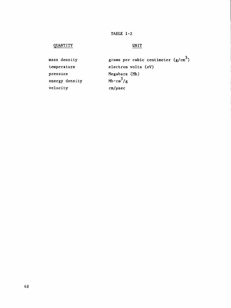
QUANTITY

mass density

temperature

pressure

energy density

velocity

TABLE I-2

UNIT

grams per cubic centimeter (g/cm3)

electronvolts (eV)

Megabars (Mb)

Mb*cm3/g

cm/psec

48

TABLE IX-1

DEFAULT COMPRESSIONGRID (dimensionless)

0.0 10-6 2 x 10-6 5 x 10-6

10-5 2 x 10-5 5 x 10-5 10-4

2 x 10-4 5 x 10

-410-3 1.5 x 10

-3

2 x 10-3 4 x 10-3 6 X 10-3 10-2

1.5 x 10-2 2.5 x 10-2 4 x 10-2 (j X 10-2

0.1 0.125 0.15 0.2

0.25 0.3 0.4 0.5

0.6 0.7 0.8 0.9

0.95 1.0 1.05 1.1

1.2 1.4 1.6 1.8

2.0 2.5 3.0 3.5

4.0 5.0 6.0 7.0

8.0 9.0 10.0 15.0

20.0 25.0 30.0 40.0

60.0 80.0 100.0 150.0

250.0 400.0 600.0 103

2 x 103 5 x K? 104 2 x 104

49

TABLE IX-2

o0.1

1

3

10

20

100

600

6000

100000

DEFAULT TEMPERATUREGRID (eV)

0.0125 0.025692

0.25 0.5

1.5 2

4 5

15 20

40 50

150 250

1000 1500

10000 20000

0.05

0.75

2.5

8

25

80

400

2500

50000

50

REFERENCESI

1.

2.

3.

4.

5.

6.

7.

8.

9.

10.

11.

Necia G. Cooper,

/

“An Invitation to Participate in the LASL Equation of

State Library,” Los Alamos Sc entific Laboratory brochure LA-79-62

(February1980).

F. Dowell, “SESAME ’83: Repor on the Los Alamos Equation-of-State

Library,v Los Alamos National L boratory report LALP-83-4 (February1983).

I

B. I. Bemett, J. D. Johnson, G. I. Kerley, and G. T. Rood, ‘Recent

Developments in the Sesame Eq ation-of-State Library,” LOS Alamos

1

ScientificLaboratory report LA- 130 (February1978).

J. Abdallah, Jr., G. I. Kerley, . I. Bemett, J. D. Johnson, R. C. Albers,

and W. F. Huebner, “HYDSES: A Subroutine Package for Using Sesame in

Hydrodynamic Codes,”

(June 1980).

Charles W. Cranfill,

Los Alamos Sesame EOS

Los Alamo’

1

Scientific Laboratory report LA-8209

‘EOSPAC: A Subroutine Package for Accessing the

Data Libra~y,H Los Alamos National Laboratory report

LA-9728-M (August 1983).

I

J. M. Hyman and M. M. Klein, “EO MOD: A SubroutinePackage for Calculating

Equation of State and Opacities “ Los Alamos National Laboratory report

LA-8502-M (October1981).

1

M. S. Shaw and G. K. Straub, ‘HYDROX:

Hydrodynamics Code,” Los Alamo Nationa

(March 1981).

The T-4 code EOSCRAY was develop d at Los

A One-DimensionalLagrangian

Laboratory report LA-8642-M

Alamos by B. I. Bennett.

INo formal documentationexists f r EOSCRAY.

G. I. Kerley, “User’s Manual fo PANDA: A Computer Code for Calculating

Equations of State,w Los Alamo National Laboratory report LA-8833-M

(November1981).

GRIZZLY uses a version of CANDID developedbyD. A. Liberman and modified

by J. D. Johnson. JThe basic phys cs is discussed in Appendix A.

Joseph Abdallah, Jr., “MIXB:

I

BCON Controller for Generating and

Maintaining Sesame Library Files of Mixture Data,” Los Alamos Scientific

Laboratoryreport LA-8219-M (Apr”l 1980).

1

51

12.

13.

14.

15.

16.

17.

18.

19.

20.

21.

22.

23.

R. C. Albers, “An Introductionto Two-TemperatureEquations of State,”

Los Alamos ScientificLaboratoryreport LA-7934-MS (July 1979).

Joseph Abdallah, Jr., ‘User’s Manual for CURVES,” Los Alamos National

Laboratoryreport LA-8844-M (October 1981).

B. I. Bemett, “On Obtaining the Zero-TemperatureEquation of State from

Shock Data,” Los Alamos National Laboratory report LA-9890-MS (January

1984).

B. I. Bennett, “A ComputationallyEfficient Expression for the Zero-

Temperature Isotherm in Equations of State,M Los Alamos ScientificLabor-

atory report LA-8616-MS (December1980).

S. L. Thompson and H. S. Lawson, ‘Improvementsthe Chart-D Radiation-

Hydrodynamic Code III: Revised Analytic Equations of State,M Sandia

National Laboratory report SC-RR-710714(March 1972).

G. I. Kerley, ‘Rational Function Method of Interpolation,”Los Alamos

ScientificLaboratory report LA-6903-MS (August 1977).

S. P. Marsh, Ed., LASL Shock Hugoniot Data (Universityof CaliforniaPress,

Berkeley, 1980).

J. D. Johnson and S. P. Lyon, “SES2D User’s Manual,” Los Alamos National

Laboratoryreport LA-9164-M (April 1982).

M. S. Hoyt, ‘User’s Manual for LASL Shock Hugoniot Data File,H Los Alamos

ScientificLaboratory report LA-7887-M (July 1979).

K. A. Gschneider,Solid State Physics ~, 275 (1964).

R. P. Feynman, N. Metropolis, and E. Teller, Phys. Rev. 7&, 1561 (1949).

R. D. Cowan and J. Ashkin, Phys. Rev. 105, 144 (1957).

52

F!L L no ME

Figure 16-1-1. Sample GRIZZLY run to generate default aluminum3716-1S1 in example 1.TCIW<X1

A- O.00.M.-,. MI.IPi- Y.76.i-30-5 .s0.03c- 1. !S.mF- z. 12.mG- 3. W.01M- 5.80.048- 1.16.05J- z. 3?.05.- 3.,8.05L- 5.00.05

RHO (MG/M3)

EOS

Figure 16-1-2. Total pressure for aluminum calculatedin example 1.The pressure is plotted versus mass density for varioustemperatures.

53

,07

,0 6

,0

,4

8

“. ,.10s“. Z..30.C4o-s.*-,. I.-a.a-6.96,~R.e. r?.m● . ,,,8.0s

Figure 16-1-3.

0

I

I

D

IIw-

n

~

—

k

,-RHO (MG/M3)

Total internalenergYfor ~lminum calculatedin examP1e 1.

,0*

,06

Figure 16-1-4.

54

RHO (M6/M3)

Totalaluminum calculated

in example 1“free energY ‘or

—

37! 6- !s1TIH 1X1

A- O. 00.00n- 5.00.03c- ! !8.mD- Z.=*D4[- 3.4WQ4r- 5.00.UIG- 1.16.03It 2.s?.05!- 3.W.B.l-5. ao. Q5N- I.le. ffiL- Z.9C-M

1!- 6.%.=N- I.r+. mO-a.mwlP- 2.?2.LW0. I .88.-

Figure 16-1-5.

,O!z

,0”

10’”

100

!0 ●

107

,0 n

10 5

10 %

80 3

!0 2

10 1

100

,0-1

,L#

,0-3 5

RHO (MG/M3)

Thermal electroniccontributionto the pressure foraluminum calculatedin example 1.

r716-lSTIDrlKl

I!.6.96.MN-I.74.C7O-6.S8Wp-2.32.m0-!. t6.V2

Figure 16-1-6.

lo~

10*

,03

Ioz

,Ot

100

,0-1

14-2

E

L

“

A

“

a

F~-

6

,0-3 ,,,8,.1 ,,”.1b-3 ,.-2 ,.-! ,.O ,.l ,o~ ,.3 ,0*

,0-6 10-~ IO-’ !0

RHO (MG/M3)

Thermal electroniccontributionto the internal energyfor aluminum calculatedin example 1.

3716- 1s1low 1x1

A- 0,00.00

;-i.m.rnG- I .16.03w .? *-51-3 %8.Ma- 5.m. v5K- 8.16K61--Z.90.M

a- 5 00.03c- 1. IC.m ,0 90- ? Q*C4

I I 111111 1 , I , ,1!”1 I , I I II,,.

r- , “s.0.

~j

y

~

~

Figure 16-1-7.

S710-lslTWIK1

A-0,00.Mm.z.9.OzC-1.18*30-5.00.03c- I.ts. mr- ?. SZ.Wc- I.w.oln- S.nwm1- 1 16*MJ- Z.I?.05K. 3.*8.95L- 5.10-G5

to 0, —--===s\\s\

Figure 16-1-8.

,0 6

10 5

,04

10 3

10 2 .

10 t

F

10”!

!O+“1RHO (MG/M3)

Thermal electroniccontributionto the free energy foraluminum calculatedin example 1.

Id’ ,,,,,m,,,,,,I,/

RHO (MG/M3)

Nuclear contributionto the pressure for aluminumcalculatedin example 1.

56

M-!. !6.mW- Z.W. E0-6. %.SP-1. m.m0-6.96.mR. Z. S2. M5-1.86.09

Figure 16-1-9.

!08

105

,0’

!03

!o~

10!

100

!0-1

10-2

10-3

// -1

I , I d,,!,,,,1! ,,,,,,1, ,!,,,,1, ULuA—uJ!0”S !0-+ 10-] 10-~ !0-’ 100 !0‘ 10 z 10 3 10 “ 10 ‘

“-5.80.0.1- 1.16. c5.I-2.3?. G5K- 3..8.05L-3. B0.05

RHO (MG/M3)

Nuclear contributionto the internal energy for—-calculatedin example 1.

37t6-!51,CJIP,K,

108

107

,06

lo~

!0’

103

!o~

,0’

,00

,0-)

]o-~

!0-3

~U4c11v ,, I ,,1”, ,,,,, ,,,,., 1,,, ”,, I ,1,,, m

s

n

L

RHO (t4G/M3)

16-1-10. Nuclear contributionto the free energy for aluminumcalculatedin example 1.

57

Figure 16-2-1. Sample GRIZZLY run to access EOS tables written inexample 1 and calculatethe principal hugoniot.

-

-

12

11

10

9

8

7

6

5

t’ ‘ ‘ ‘ ‘ ‘ ‘ ‘ ‘ ‘ ‘ ‘ ‘ ‘ ‘ ‘ ‘ ‘ ‘1

t-llllllll,ljl, 10 2 3 4 5

par;icle velocity ( km/see )

Figure 16-2-2. Comparisonof the calculatedaluminum hugoniot (solidline) of example 2 with experiment (Ref. 20) (squares).

58

FIL L 130NE

.-

gure 16-3-1. Sample GRIZZLY run to calculatethe silver EOS of example 3.

59

Figure

Figure

60

*ma-lsrTow [U8

.- 0,.ca.mB- 1 .*S.&?c- Z. W*&?0- 3.C4. W[- 1.86.03F- .390.030-5.80.03M- 8.m.031- I 18.0!J- 1.74.Wx. 2.s.04L-?.90. M

n. 3.*8.*?l-*, m.mw Y.m. m?- 0,.=,.ma- 1. lbmn- l.?+.ms- Z.3?. B1- z.5Q. mu- 3.*9.=V-9, W4.Bw-5.n0. nx- 9.a.m?- I.ls.m

16-3-2.

*COO-851IDw ,K,A-0,00. W

n. t .45.02C..Z.*.W0- 3. UO.C.?t- 8 .1S.03F- Z.m. mr,-5. oo.03M- 8,70.031- l.ts. ma- I.m.mR-. ?S2. m1.- Z.9Q. Q4

!!. 3 W.mN-v. cw. m* 5 00.0$r- 9..?s.040- 1. !a.wJn- 1.74.03S-.?.32.O5r-2. s-3.05U-1. w.mV-*,6W.V5“-5. SO.C9x.g. a.nT- I.ts.m

16-3-3.

10 7

, , , , , t I , , , , , t,0? d

RHO (MG/M3)

Total pressure for silver calculatedin example 3.

10*1= , I , , , r I I a I I 8 , (

,o~

Ioz

lot

100

10-8

IO-2

4

Total

RHO (MG/M3)

internalenergy for silver calculated

3

in example 3.

Figure

Figure

.mo-mr,- (K,

<

N-k.--mO-s. m.mF-9.a.olO-1. lwceR-1.m.m5-2.=.031-2.90.05“- 3.W.C5v- 9 6*.V5.- ,.m.m.- 9.-.05r- 1.16.05

16-3-4.

,wo-!5TTow ,<,

A- 0.00.00B-.?.9O.O3c- S.aa.oa0- 0. W.03i- It-mr- !.m.mC.-2.32*R!“- ? 90.L?41- 3.-.9!.- ...6*.DI.-s. no.mL-9. zO.m

n- 3.i6w5“- ,,7+.0s0. 2.5?.Q3?- 2.9W930- 3.98*C6n- ti. s..ms- S..ao.m1- 9.*.-(J- , ,6.C6

16-3-5.

,0 ‘

.,.

102

101

100b’=10-!

10-~

!0”3L100

\\\\

Y

k“’ “1’+

RHO (MG/M3)

Total free energy for silver calculatedin example 3.

106i= t , , , , I , I , , ( r , ! , ! , 3

,.!

10

!0

to

,0

,0

,0

,0

,(

I1, ~ $1 , , I , , , , , t

lot ,@ d

RHO (MG/M3)

Thermal electroniccontributionto the pressuresilver calculatedin example 3.

for

61

+==—==========

Figure

1,0

,0 0

.1,0

~igure 16-3-7.

,.-2

-3,0

,L+ ~H~ (MG/H3)eneKgY ‘or

t. ~he free

Thermal electronic

contribution

~i~Ver calculated

in example 3“

62

9000-1s11-,.,

.-o, oo. m8- 1.*5.*C-i?. w.o?O-s. no. o?C-1.16*O3r-.2.90.o30-5.00.03n-8, m.031-1. !6.0’4d- 1.7+.C+K- 2.32.0+L-2.90.Q4

n- SW*D4“. ..6..0!* 5.aO.mP- ,.m.m0- ! !8.05n- ,.ri.mS-.?.3?.O5T-.?.9Q.O5u- 3.w.mV-. .m.mU-5. BO.BX.s.m.mT- I Imm

Figure 16-3-8.

*coo-!srmw ,x,

&-o. m.wn- 1..5.O2C- Z.90.020-3.80.0?[- 1.16.01F- Z. S4.030-5. m.03“-0,70.031- 1.!6.54.1-1 .m.mK-.?. s?. mL-.?.90. P4

“-3. W.01N-9, U+*04O-s.w.mP-s. a.m0- 8.86.05n- 1.74.03S-z. =.tmT-z. w.nu-1. w.mV-*. w.mM-5.80.~X-9. W.M7- 1.1644

Figure 16-3-9.

,0 5

10 “

!0 3

10

10

to

‘“-’k /1- 1

!0” 10’ ,# Id

RHO (MG/M3)

Nuclear contributionto the pressure for silver in

,o~

,0!

100

,0.6

L

.~10’J lot IF 1P

RHO (MG/t43)

example

Nuclear contributionto the internal energy for silverin example 3.

3.

63

,000-1s1

Figure

Figure

10PIKI&-o. m.mB-1. w.r+c-z.9aw.?0- 5.80.=C-1.19*OIr-.?.90.o3O-5.0M03“-n.m. os1-8.16.04J- I.-*QIx-2.9. mL-2. W3.04

11.1. *n.olN-v. u!. mC-s. w.m●-s. a.mO-1.le.mR-1.74.01S- Z.3?. Q31- 2.90.-U-3.48.05v-4. w.mU- S.WW5X-9.*.057-1. !6. =

<

16-3-10.

16-3-11.

l-..—,.

~

,00

,0-1

,0-2

,0-3

100 108 IF d

RHO (MG/M3)

Nuclear contributionto the free energy for sin example 3.

7.0

6.5

6.0

5.5

5.0

4.5

4.0

3.5

3.0

I ‘ ‘ ‘ ‘ ‘ ‘ “ ‘ ‘ ‘ ‘ ‘ ‘ ‘ ‘ ‘ ‘ ‘ ‘ ‘ ‘ ‘ ‘ i

I, I , , , I , t 4 I , , I , , ,

0.0 0.5 1.0 1.5 2.0 2.5

particle velocity ( km/see )

ilver

Comparisonof the calculatedsilver hugioniot (solidline) of example 3 with experiment (Ref. 18) (squares).

16Q I I I I I

140

- 120

$ 1000-a) 805Cnm 60~

a 40

20

010 11 12 13 14 15 16

p ( g/cm3 )

Figure 16-3-12. Comparisonof the calculatedsilver hugoniot (solid line)of example 3 with experiment (Ref. 18) (squares).Pressureis plotted versus mass density.

,~~1~ I=I,=u~F.=FE,=n,..’”1[1 .1~.,:..fTl-lP=I.j1 ~ ‘;.IIldl:;;l.:~:~1 ;: 1~.’<’<’~~1.42Eo ..’””~-1~~~~ ~.’+:;;’~,..”};,~T~l,~1.....

HI-L 130NE

Figure 16-4-1. Sample run of GRIZZLY to calculatea beryllium oxide EOS.

65

6C.?9-lS1IWIK1

&- O,Qo. m9-.?.98.02C-1.16 *OS0-5.00.03C-1. 16*U4r-z. rz.wO-s. w.mI+s. m.m1- 1.18.=J-.?.32-MK-3.W.Q5L-%W*Q5

Figure 16-4-2.

6C20-lS1rnrltil

A-O,W.W0-.?.90.02c-1.16*O30-3 .M.01E- I Ibms- .?. =.m

n- 1. 18.sU- .?.9Q.EO- 6.=*MP- 1 .?!.074- a.mwlR- .?. =-mS- 1. 16*c4

Figure 16-4-3.

66

nmy I ll~m, t

RHO

Total pressure for BeO

(MG/M3)

calculatedin example 4.

101

lo~

,05

10* 7

103

,o~

101

100

Id

lo:~

,0-3,0”6 ,0-5 IO-* !0-3 lo”~ 10-1 100 10! lo~ 103 lo<

RHO (MG/M3)

Total internalenergy for BeO calculatedin example 4.

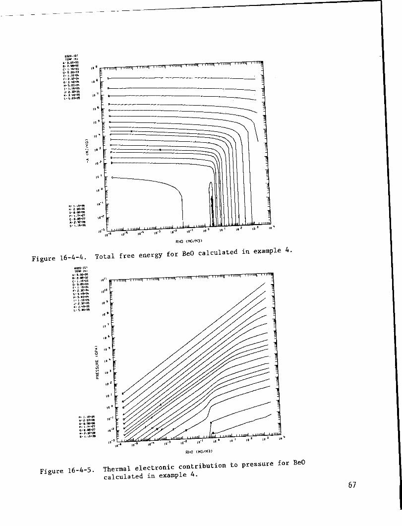
,09

,00

,0”

,0’

,0

,0

,0

,(

!

1

n-t .16.-N-2.~e-0-6.%-=P-,.7+.07.2-6.96*WR-2. *.WS-1.$6,’=

16-4-4.6WJ-KJ,Wlu$

A-o.w.m8- Z.2-Pc.,. !6.03

0-5. s0.03C-X.16*WS-2. *.Q4r,. ,..ww

H-5.9a.m,- I.16.C5J-2. ?2. D5g-3. @@5L-5.130.03

— \\ \

I I

17H0 (MG/M3)

Total free energy for BeO calculatedin examPle 4.

!0”

—

/

16-4-5.

RHO {PIG/M3)

Thermal electronic contributionto pressure ‘or ‘eo

calculatedin example 4.

.-. !.,

Figure

Figure

)!- 1.18.=H..?. wc#0-u.16.mP-1. r+.m0-8.$4.07R-.?.3.-C4s-1.ls.m

16-4-6.

6=-151rwtx,.-0,00.00

8-.?. W.Q2C-1.16,03O-5. W.03C-1.lawlr-z. wm.3-3.*8.Wn- 5.00.04!- 1.16.=a-2.32.U5K- 3.*CW4L-3. W.05

n- 1. t6. mM. Z.90. MO-6.-W=P- I.wwlo- 6.-WR- z.=.-S- 1.!6.00

16-4-7.

.

10 7

!0~

,0~

10 *

10 3

10a

10 1

,0a

10-’

Id

,0-1

0

M

N

\

80-s 10-’ !0-3 10-~ 10-! 10 0 ,0 1 !4 2 ,0 3 80 “

RHO (MG/M3)

Thermal electroniccontributionto internalenergyfor BeO calculatedin example 4.

ran

,00

80’

lo~

,05

,0*

103

lo~

101

,o~

,0-1

10-i

,0-:

s

n

0

J

~ov10-5 ,0-’+ 10-’ 10-~

RHO (MG/t43)

Thermal electroniccontributionto free energy for BeOcalculatedin example 4.

68

Figure

Figure

6.I?O - !s,IW ,K,

A- 0,00.00e-.?.m.wC- 1.16.010- 5.6m.03[- 1. 16.m;-2.3.? .04G. 3. W.Q4H- 5.a0. m8- 1. !6.05J-2.32. C6R- 3.*8.U3L- 5.80.05

/ /

RHO (MG/M3)

16-4-8. Nuclear contributionto pressure for BeO calculatedin example 4.

6b?0-1511=1X1

A-O.M.W8-2.9WWc-t .16.030-3.00.01E-1. 16.@IF-z. g.mO-3. W.W4“-5. aO. ml!-1.16.05.l-z. k?. m.- 3..8.05L-5.00. C5

l!-l. !s.mu-2.9s. mO.s. %.mP- I.-?4.O70-6. %.mR-.?. E.Q35-!. !6.03

16-4-9.

0

D

/!0-5 1O-* IO-J ,0-? ,0-1 100 ,01 ,o~ ,03 10’

RHO (MG/143)

Nuclear contributionto internal energy for BeOcalculatedin example 4.

6CZ.3-IS1,W’KB

&-o. m.mm-?.--=C-1.1-33 I❑-S. *O3[- I.16.UIF-.?.32. Wa-3. @.mH-5. M.ml-1.l~wJa-~.=.mK-3.%*W5L-5, W.C5

<

Figure I6-4-1O.

,o~

lo~

105

10*

,03

,o~

,0

,0

10”

,0’

10

P

o

b -9IO-J M

10

RHO (MG/M3)

Nuclear contributionto free

Figure 16-4-11.

in example 4.

-9

energy for BeO calculated

13.0

12.5

12.0

11.5

11.o

10.5

10.0

I 1 I I t 1 I1

9.5

9.0

8.5 II t I I t

8.0 t I I t

O.O 0.5 1.0 1.5 2.0 2.5 3.o

particle velocity ( Imhec )

Comparisonof the calculatedBeO hugoniot (solid line)of example 4 with experiment (Ref. 18) (squares).

FII- 1- DO t.4E

Figure 16-5-1. Sample run of GRIZZLY to calculatemixture of iron andmolybdenum using various schemes at a temperatureof 1 eV.

71

1:1. 1:11]1313[l@+00

Figure 16-5-2. Printed output generated in example 5.

72

STfiRT T ~El,..’,:l = 1. Ij Ij Ij FF”

-..

Figure 16-5-2.(continued).

73


74

——--—----—---—— —---------------------

75

Figure 16-6-l,(continued).

76

‘? LIST ~1-IF. ....

I-1ST 51JF. ..””-------------------------------------------------

1,=,L

1. Ij Ij Ij [1=- 1 Ij

-1. 1:11:1Ij [1=+ Ij [i

1E’ -1. [1Ij 1:1[1=+1] Ij

-1. ij [1 [1 IIE+ [! Ij

KTtl I ::.:

“ST td I :x: -1. Ij Ij [I Ij=+ [1 [1

-1. 13[1[1IIE+[11]

1E’

KF!TRE:

5RTFi E:

F:TTI+E:

5. TTFI12

– 1. [1[1t:lIj=+Ij [1 - I . Ij n II [\E+ [i [i

-------------------------------------------------

“~” Et.Jr, ,..”

EFJI, ...””

STOP

GR I Z ,~T&=&A T I PIE 1. ~ 1 ::: 5ECDH~,~

i~I=.l_l= . 1:1:::z =..,.=:= . 12:::5 I ..””D+t.l Et.fn R”y’= 1. E.4Z:

HLL DClt.4 E


77

-2Id ! I , , , , I , , , , I10-’ 10° - 10’ ld

density ( g/cma )

Figure C-1. Pressure as a functionof density at a temperatureof 1 eVfor a one to one mixture of iron and molybdenumusing thevarious mixing schemes.The iron table used was SESAME 2140and molybdenum table was SESAME 2980. The solid line isadditive volume mix, the dashed line is partial pressure mix,and the boxes are ideal mix.

78

.. .. . . . :... - .., .

. . . . —.. .-.; -.

f

- “...

; .,-,, ,

.,.. ! . . . . . ,.

i ‘“ .. ..

—J, .)- .

..

- . .. . —-.

,,

. ..-!7-. . . ,. . . . . . ;. u.....

.-. ...-.—— -- - .... .. ----- . . . . -; . .7. ‘.

-.

,. ,, . .—,.,. - .

...- ,,

. .- .,. .

.

..- .,. . . -. . . . . -... ,———

.,

..-,. ,.,,: ,,

,,. ., .

. .. ,.

,,.. ,.

. L .; - .. .,, , . . ,

,,!.

.

.

. ....

-- . !;.. .

-.. .

-. ,. :, :..

. ,.

, .. ,., ,...

. .’.. .

Ptintcd in the United SIatcs of AmerkaAvaikbk from

National Tecbnk@ Information ScrvkcUS Department of Commerce

s285 Port Roynl RoadSpringfield,VA 22161

Mkrof~k (AO1)

.——.- ----- —. ..——

,-., ,..- ‘“. . ... ~ :

.NTIS

.,.NTIS NTIS

..: ? .,NTIS

PW Range PrkcCode Pa&cRange Prk Code Page Range Price Code Pasc Ruy Pti~ Code— - .. ,. ., . ,.

! .

.

,. ..! .

W14325 A02 151.175 AOS 301.325 A14 451.475026450

A20Aw 1762Q0 A09 326.350 AM 476.300.- A21

0s147s ‘ A04 201.225 AIO 3s1.37s A16 501.52s A22076.100 A05 226250 All 376.400 A17 526550.– A23101125 AM 251.275 A12 401.42S A18 5S1.s75:; - A24126.1s0 A07 276300 A13 426.450 A19 S76.600 A25

61aS,0SA,amO - Federation of American Scientists NM 87544 Phone: (505)667-4448 E-mail:...

Documents

Transcript of 61aS,0SA,amO - Federation of American Scientists NM 87544 Phone: (505)667-4448 E-mail:...

6~~1a~~S,0SA,amO - Federation of American Scientists NM 87544 Phone: (505)667-4448 E-mail:...

Documents

Transcript of 6~~1a~~S,0SA,amO - Federation of American Scientists NM 87544 Phone: (505)667-4448 E-mail:...

61aS,0SA,amO - Federation of American Scientists NM 87544 Phone: (505)667-4448 E-mail:...

Transcript of 61aS,0SA,amO - Federation of American Scientists NM 87544 Phone: (505)667-4448 E-mail:...