1 5.6 Isobaric thermal expansion and isothermal compression (Hiroshi Matsuoka)

5.6.1 Equation of state, coefficient of thermal expansion, and isothermal compressibility

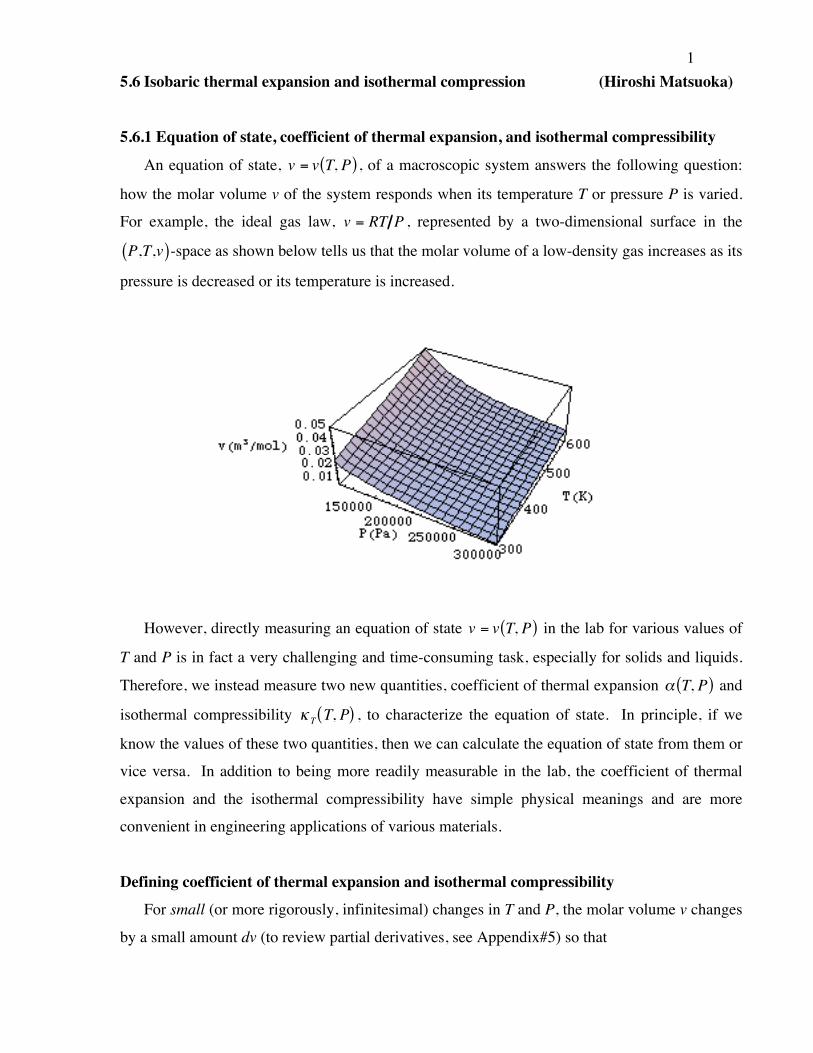
An equation of state, v = v T, P( ) , of a macroscopic system answers the following question:

how the molar volume v of the system responds when its temperature T or pressure P is varied.

For example, the ideal gas law, v = RT P , represented by a two-dimensional surface in the

!

P,T,v( )-space as shown below tells us that the molar volume of a low-density gas increases as its

pressure is decreased or its temperature is increased.

However, directly measuring an equation of state v = v T, P( ) in the lab for various values of

T and P is in fact a very challenging and time-consuming task, especially for solids and liquids.

Therefore, we instead measure two new quantities, coefficient of thermal expansion ! T, P( ) and

isothermal compressibility ! T T, P( ) , to characterize the equation of state. In principle, if we

know the values of these two quantities, then we can calculate the equation of state from them or

vice versa. In addition to being more readily measurable in the lab, the coefficient of thermal

expansion and the isothermal compressibility have simple physical meanings and are more

convenient in engineering applications of various materials.

Defining coefficient of thermal expansion and isothermal compressibility For small (or more rigorously, infinitesimal) changes in T and P, the molar volume v changes

by a small amount dv (to review partial derivatives, see Appendix#5) so that

2

dv =!v!T" # $

% & ' PdT +

!v!P" # $

% & ' TdP

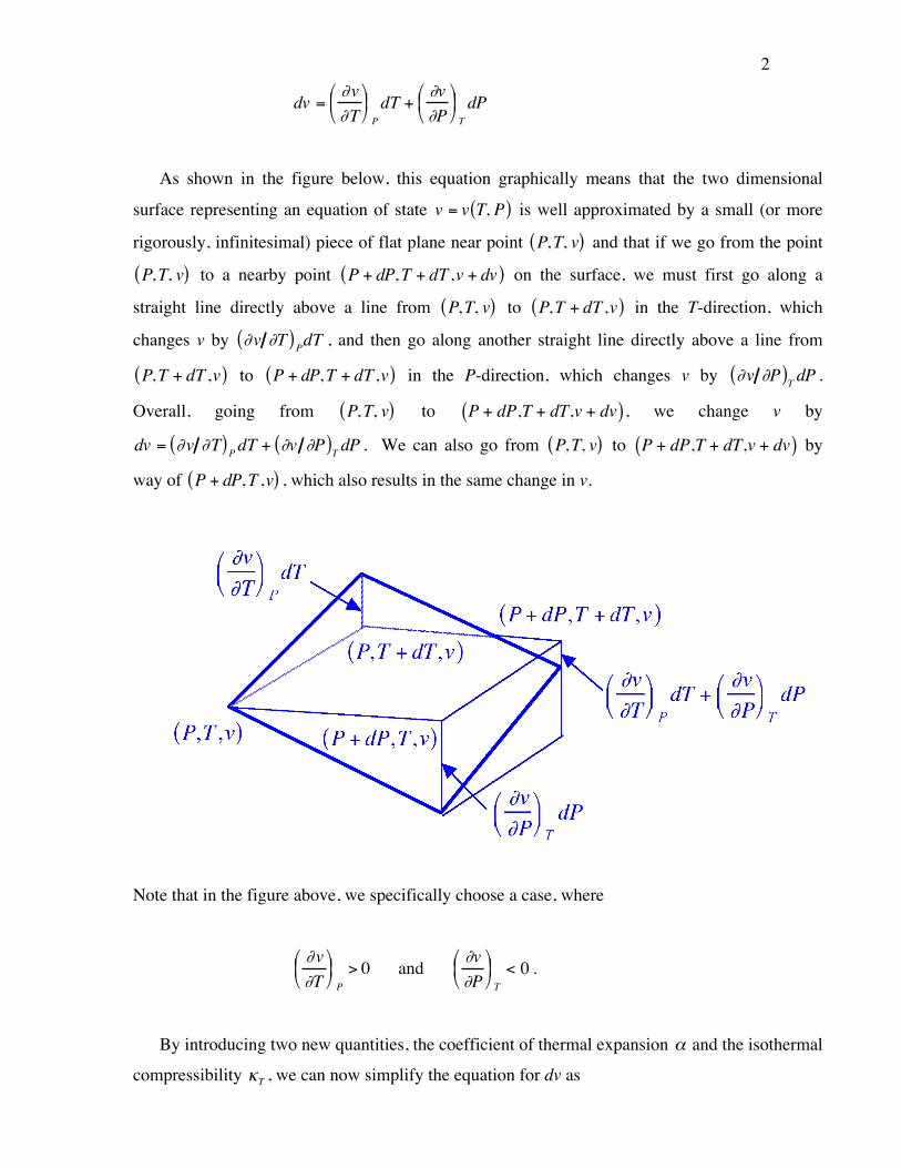
As shown in the figure below, this equation graphically means that the two dimensional

surface representing an equation of state v = v T, P( ) is well approximated by a small (or more

rigorously, infinitesimal) piece of flat plane near point P,T, v( ) and that if we go from the point

P,T, v( ) to a nearby point P + dP,T + dT ,v + dv( ) on the surface, we must first go along a

straight line directly above a line from P,T, v( ) to P,T + dT ,v( ) in the T-direction, which

changes v by !v !T( )PdT , and then go along another straight line directly above a line from

P,T + dT ,v( ) to P + dP,T + dT ,v( ) in the P-direction, which changes v by !v !P( )T dP .

Overall, going from P,T, v( ) to

!

P + dP,T + dT,v + dv( ), we change v by

dv = !v !T( )P dT + !v !P( )T dP . We can also go from P,T, v( ) to

!

P + dP,T + dT,v + dv( ) by

way of P + dP,T ,v( ) , which also results in the same change in v.

Note that in the figure above, we specifically choose a case, where

!v!T" # $

% & ' P

> 0 and !v!P" # $

% & ' T

< 0 .

By introducing two new quantities, the coefficient of thermal expansion

!

" and the isothermal

compressibility

!

"T , we can now simplify the equation for dv as

3

!

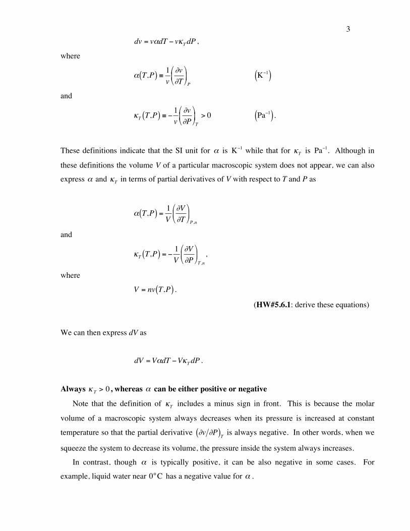
dv = v"dT # v$T dP ,

where

!

" T,P( ) # 1v$v$T%

& '

(

) * P

!

K"1( )

and

!

"T T,P( ) # $ 1v%v%P&

' (

)

* + T

> 0

!

Pa"1( ).

These definitions indicate that the SI unit for

!

" is

!

K"1 while that for

!

"T is

!

Pa"1. Although in

these definitions the volume V of a particular macroscopic system does not appear, we can also

express

!

" and

!

"T in terms of partial derivatives of V with respect to T and P as

!

" T,P( ) =1V

#V#T$

% &

'

( ) P ,n

and

!

"T T,P( ) = #1V

$V$P%

& '

(

) * T ,n

,

where

!

V = nv T,P( ) .

(HW#5.6.1: derive these equations)

We can then express dV as

!

dV =V"dT #V$T dP .

Always ! T > 0 , whereas ! can be either positive or negative

Note that the definition of

!

"T includes a minus sign in front. This is because the molar

volume of a macroscopic system always decreases when its pressure is increased at constant

temperature so that the partial derivative

!

"v "P( )T is always negative. In other words, when we

squeeze the system to decrease its volume, the pressure inside the system always increases.

In contrast, though ! is typically positive, it can be also negative in some cases. For

example, liquid water near 0°C has a negative value for ! .

4

!

" and

!

"T are related with each other

!

" and

!

"T are related with each other simply because they are derived from a single function,

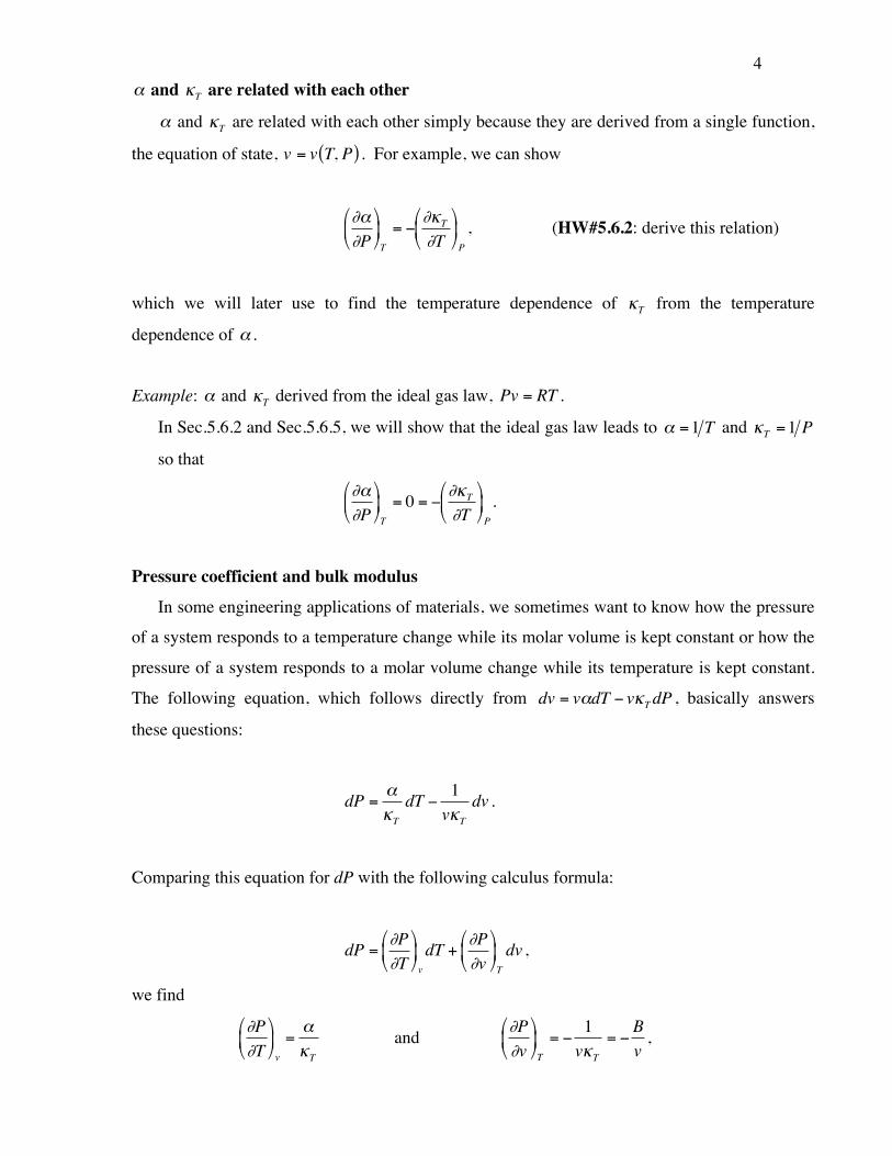
the equation of state, v = v T, P( ) . For example, we can show

!

"#"P$

% &

'

( ) T

= *"+T"T

$

% &

'

( ) P

, (HW#5.6.2: derive this relation)

which we will later use to find the temperature dependence of

!

"T from the temperature

dependence of

!

" .

Example:

!

" and

!

"T derived from the ideal gas law,

!

Pv = RT .

In Sec.5.6.2 and Sec.5.6.5, we will show that the ideal gas law leads to

!

" =1 T and

!

"T =1 P

so that

!

"#"P$

% &

'

( ) T

= 0 = *"+T"T

$

% &

'

( ) P

.

Pressure coefficient and bulk modulus

In some engineering applications of materials, we sometimes want to know how the pressure

of a system responds to a temperature change while its molar volume is kept constant or how the

pressure of a system responds to a molar volume change while its temperature is kept constant.

The following equation, which follows directly from

!

dv = v"dT # v$T dP , basically answers

these questions:

!

dP ="#T

dT $ 1v#T

dv .

Comparing this equation for dP with the following calculus formula:

!

dP ="P"T#

$ %

&

' ( v

dT +"P"v#

$ %

&

' ( T

dv ,

we find

!

"P"T#

$ %

&

' ( v

=)*T

and

!

"P"v#

$ %

&

' ( T

= )1v*T

= )Bv

,

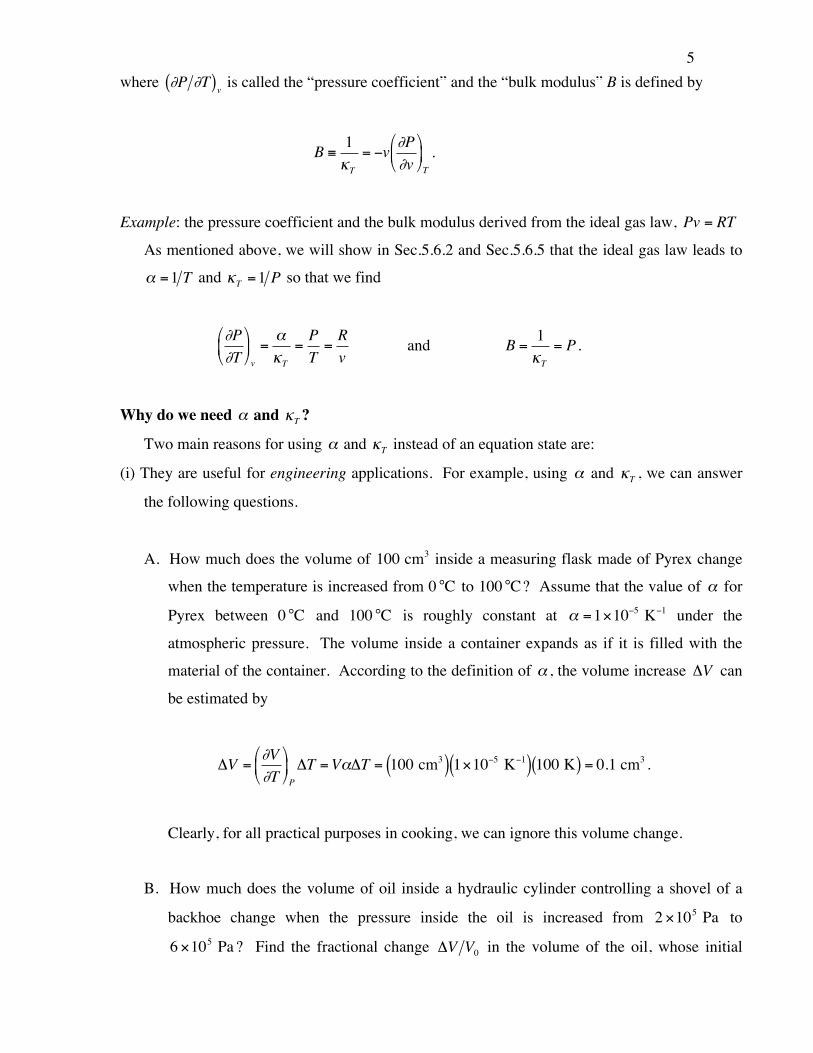
5 where

!

"P "T( )v is called the “pressure coefficient” and the “bulk modulus” B is defined by

!

B " 1#T

= $v %P%v&

' (

)

* + T

.

Example: the pressure coefficient and the bulk modulus derived from the ideal gas law,

!

Pv = RT

As mentioned above, we will show in Sec.5.6.2 and Sec.5.6.5 that the ideal gas law leads to

!

" =1 T and

!

"T =1 P so that we find

!

"P"T#

$ %

&

' ( v

=)*T

=PT

=Rv

and

!

B =1"T

= P .

Why do we need

!

" and

!

"T ?

Two main reasons for using

!

" and

!

"T instead of an equation state are:

(i) They are useful for engineering applications. For example, using

!

" and

!

"T , we can answer

the following questions.

A. How much does the volume of

!

100 cm3 inside a measuring flask made of Pyrex change

when the temperature is increased from 0

!

°C to 100

!

°C? Assume that the value of

!

" for

Pyrex between 0

!

°C and 100

!

°C is roughly constant at

!

" =1#10$5 K$1 under the

atmospheric pressure. The volume inside a container expands as if it is filled with the

material of the container. According to the definition of

!

" , the volume increase

!

"V can

be estimated by

!

"V =#V#T$

% &

'

( ) P

"T =V*"T = 100 cm3( ) 1+10,5 K,1( ) 100 K( ) = 0.1 cm3 .

Clearly, for all practical purposes in cooking, we can ignore this volume change.

B. How much does the volume of oil inside a hydraulic cylinder controlling a shovel of a

backhoe change when the pressure inside the oil is increased from

!

2 "105 Pa to

!

6 "105 Pa ? Find the fractional change

!

"V V0 in the volume of the oil, whose initial

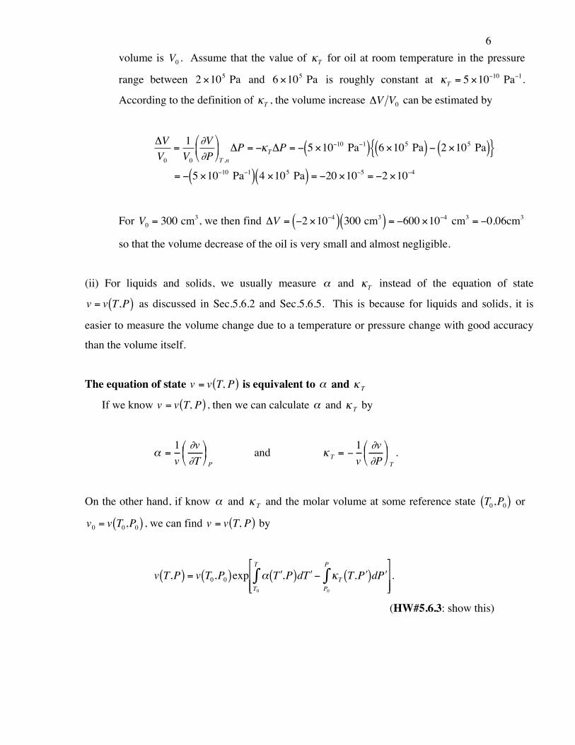
6 volume is

!

V0 . Assume that the value of

!

"T for oil at room temperature in the pressure

range between

!

2 "105 Pa and

!

6 "105 Pa is roughly constant at

!

"T = 5 #10$10 Pa$1.

According to the definition of

!

"T , the volume increase

!

"V V0 can be estimated by

!

"VV0

=1V0

#V#P$

% &

'

( ) T ,n

"P = *+T"P = * 5 ,10*10 Pa*1( ) 6 ,105 Pa( ) * 2 ,105 Pa( ){ }

= * 5 ,10*10 Pa*1( ) 4 ,105 Pa( ) = *20 ,10*5 = *2 ,10*4

For

!

V0 = 300 cm3, we then find

!

"V = #2 $10#4( ) 300 cm3( ) = #600 $10#4 cm3 = #0.06cm3

so that the volume decrease of the oil is very small and almost negligible.

(ii) For liquids and solids, we usually measure

!

" and

!

"T instead of the equation of state

!

v = v T,P( ) as discussed in Sec.5.6.2 and Sec.5.6.5. This is because for liquids and solids, it is

easier to measure the volume change due to a temperature or pressure change with good accuracy

than the volume itself.

The equation of state v = v T, P( ) is equivalent to ! and ! T

If we know v = v T, P( ) , then we can calculate ! and ! T by

! =1v

"v"T# $ %

& ' ( P

and ! T = "1v

#v#P$ % &

' ( ) T.

On the other hand, if know ! and ! T and the molar volume at some reference state

!

T0,P0( ) or

!

v0 = v T0,P0( ) , we can find v = v T, P( ) by

!

v T,P( ) = v T0,P0( )exp " # T ,P( )d # T T0

T

$ % &T T, # P ( )d # P P0

P

$'

( ) )

*

+ , , .

(HW#5.6.3: show this)

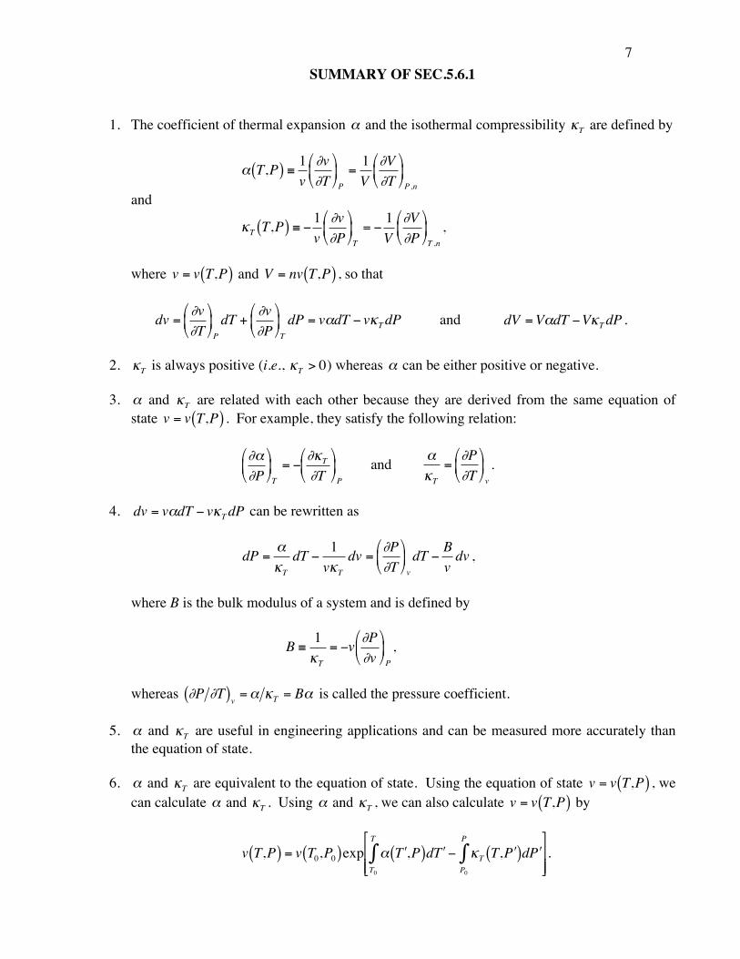
7 SUMMARY OF SEC.5.6.1

1. The coefficient of thermal expansion

!

" and the isothermal compressibility

!

"T are defined by

!

" T,P( ) # 1v$v$T%

& '

(

) * P

=1V

$V$T%

& '

(

) * P ,n

and

!

"T T,P( ) # $ 1v%v%P&

' (

)

* + T

= $1V

%V%P&

' (

)

* + T ,n

,

where

!

v = v T,P( ) and

!

V = nv T,P( ) , so that

!

dv ="v"T#

$ %

&

' ( P

dT +"v"P#

$ %

&

' ( T

dP = v)dT * v+T dP and

!

dV =V"dT #V$T dP .

2.

!

"T is always positive (i.e.,

!

"T > 0) whereas

!

" can be either positive or negative. 3.

!

" and

!

"T are related with each other because they are derived from the same equation of state

!

v = v T,P( ) . For example, they satisfy the following relation:

!

"#"P$

% &

'

( ) T

= *"+T"T

$

% &

'

( ) P

and

!

"#T

=$P$T%

& '

(

) * v

.

4.

!

dv = v"dT # v$T dP can be rewritten as

!

dP ="#T

dT $ 1v#T

dv =%P%T&

' (

)

* + v

dT $ Bvdv ,

where B is the bulk modulus of a system and is defined by

!

B " 1#T

= $v %P%v&

' (

)

* + P

,

whereas

!

"P "T( )v =# $T = B# is called the pressure coefficient.

5.

!

" and

!

"T are useful in engineering applications and can be measured more accurately than the equation of state.

6.

!

" and

!

"T are equivalent to the equation of state. Using the equation of state

!

v = v T,P( ) , we can calculate

!

" and

!

"T . Using

!

" and

!

"T , we can also calculate

!

v = v T,P( ) by

!

v T,P( ) = v T0,P0( )exp " # T ,P( )d # T T0

T

$ % &T T, # P ( )d # P P0

P

$'

( ) )

*

+ , , .

8

Answers for the homework questions in Sec.5.6.1

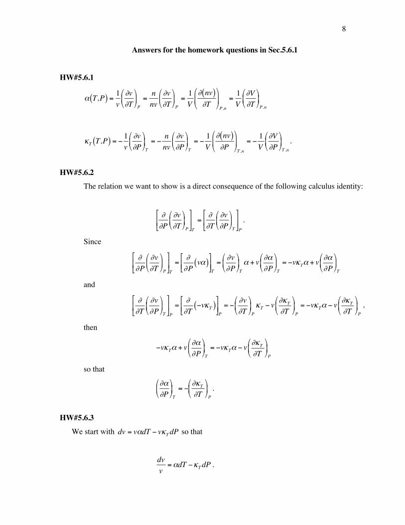
HW#5.6.1

!

" T,P( ) =1v#v#T$

% &

'

( ) P

=nnv

#v#T$

% &

'

( ) P

=1V

# nv( )#T

$

% &

'

( ) P ,n

=1V

#V#T$

% &

'

( ) P ,n

!

"T T,P( ) = #1v$v$P%

& '

(

) * T

= #nnv

$v$P%

& '

(

) * T

= #1V

$ nv( )$P

%

& '

(

) * T ,n

= #1V

$V$P%

& '

(

) * T ,n

.

HW#5.6.2

The relation we want to show is a direct consequence of the following calculus identity:

!

""P

"v"T#

$ %

&

' ( P

)

* +

,

- . T

=""T

"v"P#

$ %

&

' ( T

)

* +

,

- . P

.

Since

!!P

!v!T!

"#

$

%&P

'

()

*

+,T

=!!P

v"( )'

()*

+,T=

!v!P!

"#

$

%&T

" + v !"!P!

"#

$

%&T

= -v#T" + v!"!P!

"#

$

%&T

and

!!T

!v!P!

"#

$

%&T

'

()

*

+,P

=!!T

-v"T( )'

()*

+,P= -

!v!T!

"#

$

%&P

"T - v!"T

!T!

"#

$

%&P

= -v"T# - v!"T

!T!

"#

$

%&P

,

then

!v!T" + v#"#P"

#$

%

&'T

= !v!T" ! v#!T

#T"

#$

%

&'P

so that

!

"#"P$

% &

'

( ) T

= *"+T"T

$

% &

'

( ) P

.

HW#5.6.3

We start with

!

dv = v"dT # v$T dP so that

!

dvv

="dT #$T dP .

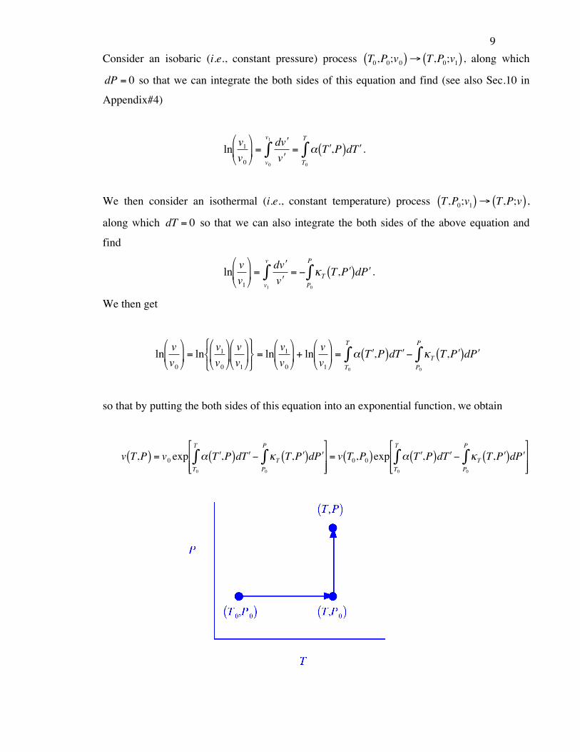
9 Consider an isobaric (i.e., constant pressure) process

!

T0,P0;v0( )" T,P0;v1( ), along which

!

dP = 0 so that we can integrate the both sides of this equation and find (see also Sec.10 in

Appendix#4)

!

ln v1v0

"

# $

%

& ' =

d ( v ( v v0

v1

) = * ( T ,P( )d ( T T0

T

) .

We then consider an isothermal (i.e., constant temperature) process

!

T,P0;v1( )" T,P;v( ),

along which

!

dT = 0 so that we can also integrate the both sides of the above equation and

find

!

ln vv1

"

# $

%

& ' =

d ( v ( v v1

v

) = * +T T, ( P ( )d ( P P0

P

) .

We then get

!

ln vv0

"

# $

%

& ' = ln

v1v0

"

# $

%

& '

vv1

"

# $

%

& '

( ) *

+ , -

= ln v1v0

"

# $

%

& ' + ln

vv1

"

# $

%

& ' = . / T ,P( )d / T

T0

T

0 1 2T T, / P ( )d / P P0

P

0

so that by putting the both sides of this equation into an exponential function, we obtain

!

v T,P( ) = v0 exp " # T ,P( )d # T T0

T

$ % &T T, # P ( )d # P P0

P

$'

( ) )

*

+ , ,

= v T0,P0( )exp " # T ,P( )d # T T0

T

$ % &T T, # P ( )d # P P0

P

$'

( ) )

*

+ , ,