5 Perturbation Theory

Generally finding the exact solution of most interesting problems is impossible or at least so dif-ficult that it is not practical to obtain it. Sometimes it is possible with a bit of work to obtain aso-called asymptotic series approximation of the solution that gives a good approximation to thesolution. In what follows I hope to provide, mostly by way of numerous examples, some insightinto this important branch of mathematics which I refer to as perturbation theory. Our goal is to ex-amine several examples including the asymptotic analysis of solutions of algebraic, transcendental,differential equations and the evaluation of integrals.

5.1 Preliminary material

The binomial Theorem states

(a+ b)n = an + nan−1b+n(n− 1)

2!an−2b2 + · · · . (5.1.1)

If n is a positive integer this formula terminates and we have the more familiar formula

(a+ b)n = an + nan−1b+n(n− 1)

2!an−2b2 + · · ·+ bn.

More generally for n ∈ R the series is infinite and converges for

∣∣∣∣ ba∣∣∣∣ < 1 and diverges otherwise.

As examples consider

(a+ b)1/2 =a1/2 +1

2a−1/2b+

(12

) (−12

)2!

a−3/2b2 + · · · (5.1.2)

(a+ b)−1 =a−1 − a−2b+ a−3b2 − a−4b3 + · · · . (5.1.3)

We will also use the classical Taylor series (and Taylor Polynomial) expansion for a smoothfunction which expanded about x = x0 is given by

f(x) =∞∑n=0

f (n)(x0)

n!(x− x0)

n. (5.1.4)

1

Examples with x0 = 0 include

ex =∞∑n=0

xn

n!, (5.1.5)

sin(x) =∞∑n=0

(−1)nx(2n+1)

(2n+ 1)!(5.1.6)

cos(x) =∞∑n=0

(−1)nx(2n)

(2n)!. (5.1.7)

We are interested inlimε→0

f(ε), ε > 0.

We will usually assume that ε > 0 in order to minimize confusion that might arise otherwise, e.g.,

limε↓0e−1/ε = 0, lim

ε↑0e−1/ε =∞.

We are also interested in the case when the limit exists (i.e., it does not have an essential singularitylike sin(1/ε)). Thus we consider the cases

f(ε)→ 0,

f(ε)→ A,

f(ε)→∞,

as ε→ 0, 0 < A <∞.

If f(ε) → 0,∞ as ε → 0 then we are also interested in the rate at which the limit is approached,e.g.,

limε→0

sin(ε) = 0, limε→0

(1− cos(ε)) = 0, limε→0

(ε− sin(ε)) = 0, limε→0

[ln(1 + ε)]4 = 0, limε→0

e−1/ε = 0.

In order to determine the rate at which such a limit is achieved we introduce the concept of gaugefunctions. The simplest such functions are the powers of ε which for ε < 1 satisfy

1 > ε > ε2 > · · · , ε−1 < ε−2 < ε−3 < · · · .Thus for example we can compute, using Taylor series or using L’Hospital’s rule

limε→0

sin(ε)

ε= lim

ε→0

(1− ε

2

3!+ε4

5!− · · ·

)= 1

limε→0

(1− cos(ε))

ε2=

1

2!

limε→0

(ε− sin(ε))

ε3=

1

3!

limε→0

[ln(1 + ε)]4

ε4= lim

ε→0

(1− ε

2+ε2

3+ · · ·

)= 1.

2

Note also that functions like f(ε) = e−1/ε go to zero faster than any power of ε, i.e., byL’Hospital’s rule

limε→0

e−1/ε

εn= lim

x→∞

xn

ex= lim

x→∞

n!

ex= 0.

Furthermore, f (n)(0) = 0 for all n. For example, f ′(ε) = e−1/ε/ε2, and once again usingL’Hospital’s rule

f ′(0) = limε→0

e−1/ε

ε2= lim

x→∞

x2

ex= lim

x→∞

2

ex= 0.

Thus f cannot be expanded in a taylor series about ε = 0.On the other hand the function f(ε) = e1/ε → ∞ as ε → 0 and this limit is faster than any

power of 1/ε, i.e.,

limε→0

e1/ε

1/εn= lim

x→∞

ex

xn= lim

x→∞

ex

n!=∞.

We also have slowly converging functions like f(ε) = ln(1/ε) which goes to zero slower thanany power of 1/ε. Namely,

limε→0

ln(1/ε)

ε−α= lim

x→∞

ln(x)

xα= lim

x→∞

1

αxα= 0.

So, in addition to all powers of ε (i.e., εj , for j = · · · ,−2,−1, 0, 1, 2, · · · we also might needfunctions like e±1/ε and ln(1/ε), ln(ε), etc.

A very useful notation that we will use often is the “Big Oh” and “Little Oh” notation.

Definition 5.1. We say that f(ε) = O(g(ε)) as ε→ 0 if

limε→0

f(ε)

g(ε)= A, 0 < |A| <∞. (5.1.8)

We say that f(ε) = o(g(ε)) as ε→ 0 if

limε→0

f(ε)

g(ε)= 0. (5.1.9)

Examples of “Big-Oh” include

cos(ε) = O(1), 1− cos(ε) = O(ε2), tanh(ε) = O(ε), sec(ε) = O(1),ε3/2

sin(ε)= O(ε1/2).

One of the main uses of the “little-oh” notation comes from the fact that sometimes it may behard to determine the exact rate of convergence but it is sufficient to determine whether the rate isfaster or slower than a given gauge. Examples of “little-h” include

sin(ε) = o(1), sin(ε) = o(ε1/2), cos(ε) = o(ε−1), e−1/ε = o(ε−10−8

), ln(1/ε) = o(ε−.000001).

Since we may not be able to use only powers of ε to identify the rate of convergence of afunction, we are lead to supposing that we have a general set of gauge functions.

3

Definition 5.2. We say thatN∑

n=0

cnfn(ε)

is an asymptotic expansion of f(ε) at ε = 0 if the following hold:

1. The sequence {fn}, n = 0, · · · , (N + 1), is a gauge sequence; i.e., fn(ε) = o(fn−1(ε)) asε→ 0 for n = 1, · · · , (N + 1), and

2. we have

f(ε)−N∑

n=0

cnfn(ε) = O(fN+1(ε)) as ε→ 0.

As an example, if f(ε) has (N +1) continuous derivatives at ε = 0 then it can be approximated(near ε = 0) by a Taylor polynomial of degree N

f(ε) = f(0) + f (1)(0)ε+ · · ·+ f (N)(0)εN/N ! + O(εN+1).

The error term is given by

f (N+1)(η)

(N + 1)!εN+1, for some 0 < η < ε.

Here the gauge functions are fn = εn.

Theorem 5.1 (Fundamental Theorem of Perturbation theory). If an asymptotic expansion sat-isfies

A0 + A1ε+ · · ·ANεN + O(εN+1) ≡ 0,

for all sufficiently small ε and the coefficients {Aj} are independent of ε, then

A0 = A1 = · · · = AN = 0.

5.2 Algebraic Equations

Example 5.1. We would expect that the roots of the quadratic equation

x2 − 2x+ .001 = 0

would be close to the roots x = 0 and x = 2 of x2 − 2x = 0 since .001 is small. The question iscan we say approximately how close they are. To answer this we consider obtaining an asymptoticexpansion for the roots of the more general problem

x2 − 2x+ ε = 0 for ε 1

where ε 1 means that ε is much less than 1.For this example let us let x1 = 0, x2 = 2 and note that the exact solutions to the perturbed

problem arex1(ε) = 1−

√1− ε, x2(ε) = 1 +

√1− ε.

4

Then based on the binomial theorem given in (5.1.1) with a = 1, b = −ε and n = 1/2 whichimplies

√1− ε = 1− 1

2ε− 1

8ε2 − · · · .

Thus we can write

x1(ε) =1

2ε+

1

8ε2 +

1

16ε3 + · · · ,

and

x2(ε) = 2− 1

2ε− 1

8ε2 − 1

16ε3 + · · · .

So we can easily the rate at which the perturbed roots converge to the exact roots at ε = 0.An important question is whether or not this is actually an asymptotic expansion. If we can

show that the series represents a convergent power series, then it is an asymptotic series.One of the best methods to check whether a power series is convergent is the ratio test which

states ∞∑n−1

uk converges if limk→∞

uk+1

uk< 1.

For our example we have the kth term given by

(1/2)(1/2− 1) · · · (1/2− k)(−ε)kk!

so

limk→∞

(k + 1)st termkth term

= limk→∞

(k + 1/2)

(k + 1)ε = ε

so the series converges for 0 < ε < 1.Thus would not be a very useful method if we had to use the quadratic formula as we did above.

Let us consider a more direct method – the method of regular perturbation theory. We suspect thatthere is an asymptotic series in the form

x(ε) = a0 + a1ε+ a2ε2 + · · · .

We substitute this formal series into the perturbed equation and appeal to (5.1) by successivelysetting the terms corresponding to powers of ε equal to zero.

For this example we would have

(a0 + a1ε+ a2ε2 + · · · )2 − 2(a0 + a1ε+ a2ε

2 + · · · ) + ε = 0

or, collecting powers of ε,

[a20 + 2a0a1ε+ (a1 + 2a0a2)ε

2 + · · · ]− 2[a0 + a1ε+ a2ε2 + · · · ] + ε = 0

or(a2

0 − 2a0) + (2a0a1 − 2a1 + 1)ε+ (a21 + 2a0a2 − 2a2)ε

2 + · · ·

5

which gives

ε0 : a20 − 2a0 = 0, ⇒ a0 = 0, 2,

ε1 : 2a0a1 − 2a1 + 1 = 0, ⇒ a1 =−1

2(a0 − 1),

ε2 : a21 + 2a0a2 − 2a2 = 0, ⇒ a2 =

−a21

2(a0 − 1).

If we take a0 = 0 then this gives

a1 =−1

2(0− 1)=

1

2, a2 =

−(1/2)2

2(0− 1)=

1

8,

and for a0 = 2 then this gives

a1 =−1

2(2− 1)= −1

2, a2 =

−(1/2)2

2(2− 1)= −1

8,

in agreement with our calculations above.Sometimes we might want to use the knowledge that the result can be given in a power series

expansion, i.e., that

aj =x(j)(0)

j!, where x(j)(0) =

dj

dεjx(ε)

∣∣ε=0.

So in this case we compute

d

dεf(x(ε)) =

d

dε(x(ε)2 − 2x(ε) + ε) = 2x(ε)

dx

dε(ε)− 2

dx

dε(ε) + 1 = 0

which, for x(0) = 0 givesdx

dε(0) =

1

2

and, for x(0) = 2 givesdx

dε(0) = −1

2.

We could continue but I think you get the idea.

Unfortunately it is very common that a regular asymptotic expansion does not suffice. Considerthe following example.

Example 5.2. Consider the quadratic equation

εx2 + x+ 1 = 0.

For every nonzero ε this equation has two roots but for ε = 0 the equation becomes x+1 = 0 whichhas only one root x = −1. Thus we say that there is a singularity in the roots of the perturbedequation at ε = 0 (hence the name “singular perturbation problem”).

If we proceed as we did in Example 5.1 by assuming an expansion

x(ε) = a0 + a1ε+ a2ε2 + · · · ,

6

then we getε(a0 + a1ε+ a2ε

2 + · · · )2 + (a0 + a1ε+a2ε

2 + · · · ) + 1 = 0,

or(a0 + 1) + ε(a1 + a2

0) + · · ·which implies

a0 = −1, a1 = −a20, · · · ⇒ x(ε) = −1− ε+ · · · .

But this only gives information about one perturbed root.The exact roots are

x(ε) =1

2ε

(−1±

√1− 4ε

). (5.2.1)

If we once again apply the binomial theorem with a = 1, b = −4ε and n = 1/2 then we have

(1− 4ε)1/2 = 1− 2ε+(1/2)(−1/2)

2!16ε2 + · · ·

= 1− 2ε− 2ε2 + · · ·

Thus using the exact solutions (5.2.1) with the plus sign we arrive at

x(ε) =−1 + 1− 2ε− 2ε2 + · · ·

2ε= −1− ε+ · · ·

just as above. But when we use (5.2.1) with the minus sign we get

x(ε) =−1− 1 + 2ε+ 2ε2 + · · ·

2ε= −1

ε+ 1 + ε+ · · · .

Thus the two roots go into powers of ε but one starts out with ε−1.Thus we see that we cannot expect to have asymptotic expansions only in the form

x(ε) = a0 + a1ε+ a2ε2 + · · · ,

and we need additional information to determine the form of the expansions.This is one of the main ideas in the area of singular perturbation theory.We could have argued that since the number of roots of the unperturbed problem is less than

the number of roots of the perturbed problem we should expect that some perturbed roots must goto infinity as ε→ 0. With this in mind we might seek an expansion in the form

x(ε) =y

εν, for ν ≥ 0.

Substituting into our equation

0 = f(x(ε)) = εx(ε)2 + x(ε) + 1 = ε( yεν

)2

+( yεν

)+ 1

we end up withε1−2νy2 + ε−νy + 1 = 0.

7

In order to see that one root must go to infinity (like 1/ε) we give a heuristic argument thatsuggests this should be the case. Let x1(ε), x2(ε) be the two roots. Then

ε[x− x1(ε)][x− x2(ε)] ≡ 0.

If we multiply out the terms and recall that for every ε this must be εx2 + x+ 1 = 0 we get

εx2 − [x1(ε) + x2(ε)]x+ x1(ε)x2(ε) = 0

or−ε[x1(ε) + x2(ε)] = 1

andεx1(ε)x2(ε) = 1.

Definition 5.3. We say that f ∼ g if and only iff(ε)

g(ε)→ 1 as ε→ 0.

Now since we expect x1(ε) ∼ 1 which implies that x2(ε) ∼ b/ε where b is some constant.

We have just learned that we do not obtain a regular perturbation problem when the number ofroots is less for the unperturbed problem than for the perturbed problem. This is not the only waya singular problem can arise from these types of perturbation problems. The next example showsthat if the original (unperturbed) problem has multiple roots there can also be a problem.

Example 5.3. Consider the quadratic equation

P (ε) = x2 − 2εx− ε = 0.

For this problem no roots are lost when ε = 0, namely, x = 0 is a double root. If we try to proceedto obtain an asymptotic expansion for the roots as a regular perturbation expansion

x = a0 + a1x+ a2x2 + · · · , (5.2.2)

then when we truncate at N = 2 we get

a20 + (2a0a1 − 2a0 − 1)ε+ (a2

1 + 2a0a2 − 2a1)ε2 + O(ε3) = 0.

Which impliesa2

0 = 0, 2a0a1 − 2a0 − 1 = 0, a21 + 2a0a2 − 2a1 = 0.

This implies thata0 = 0,

and then that −1 = 0 which is a contradiction.Thus no roots of P (ε) have the form (5.2.2). Just as in the previous examples we could apply

the quadratic formula to find out what the form of the roots is but this really defeats the purposeof our investigation. In particular for polynomials of degree greater than or equal five there is noformula like the quadratic formula to use.

8

Let us consider the following line of reasoning. We know that there must be two roots whichwe denote by x1(ε) and x2(ε) which must approach zero as ε → 0. Let us assume that the zerossatisfy

xj(ε) ∼ εpb0, p > 0, β0 �= 0.

Just as in the last example, let us make the change of variables

x(ε) = εpw(ε), w(0) �= 0.

Then we getQ(w, ε) ≡ P (ε) = ε2pw2(ε)− 2εp+1w(ε)− ε = 0.

As ε goes to zero the largest of {ε2p, εp+1, ε1} is the one with the smallest exponent (since a fractionraised to a higher power is smaller). Thus to find the dominant term we must determine the smallestof these exponents.

Note that if 1/2 < p < 1 then

min{2p, p+ 1, 1} = 1

which givesε2w2(ε)− 2ε2w(ε)− ε = 0.

But if we divide by ε and let ε tend to zero we are left with −1 = 0 which is a contradiction.If, on the other hand, 0 < p < 1/2 then

min{2p, p+ 1, 1} = 2p

which, on multiplying by ε−2p, gives

0 ≡ ε−2pQ(w, ε) = w2(ε)− 2ε−p+1w(ε)− ε1−2p ∼ w2(ε) ∼ w2(0) ⇒ w(0) = 0

which, once again, is a contradiction.The only other possibility is that p = 1/2. In this case we have

0 ≡ ε−1Q(w, ε) = w2(ε)− 2ε1/2w(ε)− 1 ∼ w(0)− 1, ⇒ w(0) = ±1.

This could work.Note that with this substitution the resulting polynomial in w is

w2(ε)− 2ε1/2w(ε)− 1 = 0.

Now working with a fractional power of ε is not so convenient so let us make one final adjust-ment and set

β = ε1/2

to obtain the regular perturbation problem

w2 − 2βw − 1 = 0,

for which we seek an expansion for β ∼ 0 in the form

w(β) = b0 + b1β + b2β2 + · · ·+ bNβN + O(βN+1), b0 �= 0.

9

Substitution in the polynomial gives

b20 − 1 = 0,

2b0b1 − 2b0 = 0,

b21 + 2b0b2 − 2b1 = 0,

...

which implies

b0 = ±1,

b1 = 1,

b2 = ±1/2,

...

Thus we obtain the expansions

x1(ε) = ε1/2 + ε+1

2ε3/2 + O(ε2),

x2(ε) = −ε1/2 + ε− 1

2ε3/2 + O(ε2).

Immediately following this example we turn to the problem of determining the asymptoticdevelopment of a wide class of algebraic equations. This discussion will include a method fordetermining the value of p as in this example. Since we have a simple example here let us take thisopportunity to show graphically how the general method works.

To determine the minimal value for the set {ε2p, εp+1, ε1} we proceed as follows: In the (p, q)plane, plot the lines q = 2p, q = p+ 1, q = 1. These lines will intersect in several places. Namely,two of the lines intersect at (2/1, 1) and two others intersect at (0, 1). Each of these points onintersection determine the asymptotic behavior of one branch of the roots of our equation.

The three lines form two intersections

10

At this point we present a quite general result for a class of singular perturbation problems. Weconsider polynomial equations of the form

P (x, ε) =(1 + b0ε+ c0ε2 + · · · ) + A1ε

α1(1 + b1ε+ c1ε2 + · · · )x (5.2.3)

+ · · ·+ Anεαn(1 + bnε+ cnε

2 + · · · )xn = 0,

where αi are rational, bi, ci, etc are constants and (1 + biε+ · · · ) are regular asymptotic series, i.e.,they have the form

a0 + a1ε+ · · ·+ aNεN +RN+1(ε), with RN+1(ε) = O(εN+1).

We note that with this definition P (x, ε) can have roots that approach zero, a finite number orinfinity (see the homework problems).

Much of the material in this section is taken from the Dover book [13] including the followingTheorem.

Theorem 5.2. Each zero x(ε) of (5.2.3) is of the form

x(ε) = εpw(ε), w(0) �= 0 (5.2.4)

where w(ε) is a continuous function of ε for ε ∼ 0.

Sketch of Proof. If x(ε) = εpw(ε), w(0) �= 0 then P (εpw, ε) can be written as

P (εpw, ε) = Q(w, ε) + ε(b0 + εα1+pb1A1w + · · ·+ εαn+npbnAnwn) + · · · ,

whereQ(w, ε) = 1 + εα1+pA1w + · · · εαn+npAnw

n.

The main point is that the exponents

E = {0, α1 + p, · · · , αn + np} (5.2.5)

determines a set of, so-called, proper values {p1, p2, · · · , pm}. These numbers are determined asfollows: Draw the graphs of the lines q = αj + jp in the (p, q) plane. Starting on the right, wenote that for p sufficiently large the smallest exponent will be 0. As p decreases, we imagine avertical line moving with us through the graphs of the various lines, there will be a first point atwhich (at least) two lines intersect at a point (p1, 0) (here e1 = 0). At this point one and only oneline will have the largest slope n1. Now continue to the left along the intersection of your verticalline and the line with maximum slope until you encounter the next point of intersection with oneof the set of lines. This point is denoted (p2, e2). The slopes, at this point, range from a minimumof n1 to a maximum of n2. Continue in the same fashion until the last and smallest proper valuepm is reached (i.e., there are no more intersection lines to the left). At least one of the lines thatintersect at this last point must have the maximum slope of all the lines which is n. In this way wehave generated a set of pairs {(pj, ej)}mj=1

Now for each j define the polynomials

T (j)(w, ε) = ε−ejP (εpjw, ε).

11

Each T (j)(w, ε) can be written as

T (j)(w, ε) = T (j)(w) + E(j)(w, ε)

whereT (j)(w) = Anj (wnj + · · ·+Bjw

nj−k) , E(j)(w, 0) = 0.

We note that if the nonzero roots of T (j)(w) are given by xk for k = 1, · · · , nj , then T (j)(w, ε)has nj roots denoted by xk(ε) satisfying

limε→∞

xk(ε) = xk, k = 1, · · · , nj.

That is, the roots of T (j)(w, ε) approach the roots of T (j)(w) as ε→∞.Unfortunately, the non-zero roots of T (j)(w, ε) need not be regular: the α’s and the associated

proper values and exponents, (pj, ej), may be non-integer rational or T (j)(w) may have repeatedroots. Thus to obtain regular expansions, new parameters must be introduced. Namely, we intro-duce a new parameter β by

ε = βqj (5.2.6)

where

qj = lcd{0, α1 + pj, · · · , αn + npj}, lcd means least common denominator.

then letR(j)(w, β) = T (j)(w, βqj) = β−qjejP (βqjpjw, βqj).

The roots of T (j)(w, ε) are identical to those of R(j)(w, β) but the nonzero roots of R(j)(w, β) willhave a regular expansion in w of the form

w(β) = b0 + b1β + · · ·+ bNβN + O(βN+1).

SUMMARY:

Every root of (5.2.3) can be expressed in the form (5.2.4). The set of exponents(5.2.5) determines a set of proper values {p1, · · · , pm}. For each proper value we in-troduce a new parameter β through (5.2.6) and an associated polynomialR(j)(w, β).The simple non-zero roots R(j)(w, β) have regular perturbation expansions in β.The total number of non-zero roots of all the R(j)(w, β) is n. These yield expan-sions for each of the roots of (5.2.3).

Example 5.4. At this point an example showing how to choose the proper values is probably thebest way to see what this means. Consider

P (x, ε) = 1 + x3 + ε6x6 + 2ε9x7 + ε12x8 + ε18x9.

12

The substitution of x = εpw gives

P (εpw, ε) = 1 + ε3pw3 + ε6+6pw6 + 2ε9+7pw7 + ε12+8pw8 + ε12+8pw9,

so the set of exponents is

E = {0, 3p, 6 + 6p, 9 + 7p, 12 + 8p, 12 + 8p}.From the graph we can read off the proper values pj and the minimal exponents ej .

-6 -4 -2 0 2-40

-30

-20

-10

0

10

20

30

(0,0)

(-2,-6)

(-3,-12)

(-6,-36)

Determination of the Proper values

We obtain

1. (0, 0) : T (1)(w, ε) = ε0P (ε0w, ε) = 1 + w3 + ε6w6 + 2ε9w7 + ε12w8 + ε18w9

2. (−2,−6) : T (2)(w, ε) = ε6P (ε−2w, ε) = w3 + w6 + 2εw7 + ε2w8 + ε6(1 + w9)

3. (−3,−12) : T (3)(w, ε) = ε12P (ε−3w, ε) = w6 + 2w7 + w8 + ε3(w3 + w9) + ε12

4. (−6,−36) : T (4)(w, ε) = ε36P (ε−6w, ε) = w8 + w9 + 2ε3w7 + ε6w6 + ε18w + ε36

Example 5.5. Let us consider the following problem in some detail

P (x, ε) = 1− ε+ ε(2 + 3ε2)x− ε−3(16− ε)x4 + ε2(4− ε+ ε3)x6.

1. Set x = εpw and determine the exponents E = {0, 1 + p,−3 + 4p, 2 + 6p} gathered from

P (εp, ε) = 1− ε+ ε1+p(2 + 3ε2)w − ε−3+4p(16− ε)w4 + ε2+6p(4− ε+ ε3)w6.

2. Determine the proper values and the polynomials T (j)(w, ε).

-4 -3 -2 -1 0 1 2-20

-15

-10

-5

0

5

10

(3/4,0)

(-5/2,-13)

13

Determination of the Proper values

(a) (3/4, 0): T (1)(w, ε) = 1− ε+ ε7/4(2 + 3ε2)w − (16− ε)w4 + ε13/2(4− ε+ ε3)w6.

(b) (−5/2,−13): T (2)(w, ε) = ε13(1− ε)+ ε23/2(2+3ε2)w− (16− ε)w4 +(4− ε+ ε3)w6.

3. For each j determine qj , set ε = βqj and compute the polynomials R(j)(w, β):

(a) ε = β4: R(1)(w, β) =β−q1e1P (βq1p1w, βq1) = 1 + β4 + β7(2 + 3β8)w − (16− β4)w4

+ β26(4− β4 + β12)w6.

(b) ε = β2: R(2)(w, β) =β−q2e2P (βq2p2w, βq2) = β26(1− β2) + β23(2 + 3β4)w − (16− β2)w4

+ β26(4− β2 + β6)w6..

4. Each R(j)(w, β) has non-zero roots of the form

w(β) = b0 + b1w + · · ·+ bNβN + O(βN+1). (5.2.7)

Substitute (5.2.7) into R(j)(w, β) ≡ 0, collect and equate to zero coefficients of like powersof β. Solve, one-by-one, for the unknowns b0, b1, · · · .

(a) For j = 1 the root will have the form w(β) = b0 + b4β4 + O(β7) from part 3 .

We have

0 = R(1)(w, β) =1− β4 + O(β7)− (16− β4)(b0 + b4β4 + O(β7))4 + O(β7)

=1− β4 − (16− β4)(b40 + 4b30b4β4) + O(β7)

=1− β4 − 16b40 − 64b30b4β4 + b40β

4 + O(β7).

Setting like powers of β to zero we arrive at

1− 16b40 = 0 ⇒ b0 =

(1

16

)1/4

=1

2e(k−1)iπ/2, k = 1, 2, 3, 4.

and

−1− 64b30b4 + b40 = 0, ⇒ b4 =(1− b40)−64b30

=(1− 1/16)b0−4

= −15

64b0

where we have multiplied the top and bottom by b0 and used the fact that b40 = 1/16.

14

(b) For j = 2 the root will have the form w(β) = b0 + b2β2 + O(β4).

Once again we have We have

0 = R(2)(w, β) =(4− β2 + β6)(b0 + b4β2 + O(β4))6 − (16− β2)(b0 + b4w

2 + O(β4))4

+ O(β4)

=(4− β2)(b60 + 6b50b2β2 + O(β4))− (16− β2)(b40 + 4b30b4β

2) + O(β4)

=(4b60 − 16b40) + (24b50b2 − b60 − 64b30b2 + b40)β2 + O(β4).

From this we conclude that

4b60 − 16b40 = 0 (the nonzero values satisfy) b20 = 4, ⇒ b0 = 2(−1)k, k = 5, 6,

and

0 = 24b50b2 − b60 − 64b30b2 + b40 ⇒ (16)(8)b2b0 = 48 ⇒ b2 =3b032.

5. Finally we write down the roots xj(ε) for j = 1, 2, 3, 4, 5, 6.

(a) xk(ε) =1

2e(k−1)iπ/2ε3/4

(1−

(15

64

)ε+ O(ε7/4)

)for k = 1, 2, 3, 4.

(b) xk(ε) = 2(−1)kε−5/2

(1 +

(3

32

)ε+ O(ε2)

)for k = 5, 6.

Example 5.6. Consider the equation

P (x, ε) = 1− 2x+ x2 + εx5 = 0.

1. For this problem we seek x = εpw so we get

P (εpw, ε) = 1− 2εpw + ε2pw2 + ε1−5pw5

andE = {0, p, 2p, 1 + 5p}

-0.5 0 0.5-2

-1.5

-1

-0.5

0

0.5

1

1.5

2

(0,0)

(-1/3,-2/3)

Determination of the Proper values

15

2. Now for j = 1, 2 we try to carry out the procedure described above.

(a) For j = 1 we have (0, 0) and

T (1)(w, ε) = ε0P (ε0w, ε) = 1− 2w + w2 + εw5.

(b) For j = 2 we have (−1/3,−2/3) and

T (2)(w, ε) = ε2/3P (ε−1/3w, ε) = ε2/3 − 2ε1/3w + w2 + w5.

3. Determine qj and set ε = βqj .

(a) For j = 1 we run into trouble. q1 = lcd{0, 1} = 1 so ε = β and

R(1)(w, β) = 1− 2w + w2 + βw5.

If we try a regular perturbation series w = b0 + b1w + · · · we arrive at

1− 2 b0 − 2 b1 β − 2 b2 β2 +

(b0 + b1 β + b2 β

2)2

+ β(b0 + b1 β + b2 β

2)5

and the coefficients of β0 is 1− 2 b0 + b02 which has a double root 1 so we see that this

is not a regular perturbation and we must proceed differently.

(b) For j = 2 we have q2 = lcd{0,−1/3,−2/3} = 3 so ε = β3 and

R(2)(w, β) = β2 − 2βw + w2 + w5.

At this point we stop and begin again.

Because of the double root must seek

w = 1 + βνu, u = u0 + u1β + u2β2 + · · · , u0 �= 0.

Thus we obtain

T (1)(1 + βνu, β) =1− 2(1 + βνu) + (1 + βνu)2 + β(1 + βνu)5

=1− 2(1 + βνu) + (1 + 2βνu+ β2νu2) + β(1 + 5βνu+ 10β2νu2 + · · · )

=β + 5βν+1u+ β2ν(1 + 10β)u2 + 10β1+3νu3 + 5β1+4νu4 + β1+5νu5.

The set of exponents is

E = {1, 2ν, ν + 1, 3ν + 1, 4ν + 1, 5ν + 1}.

16

-2 -1 0 1 2-2

-1

0

1

2

3

(-1/3,-2/3)

(1/2,1)

Determination of the Proper values

There are two proper values (p1, e1) = (1/2, 1) and (p2, e2) = (−1/3,−2/3)

1. For j = 1 multiply by β−1 and we have

1 + 5β1/2u+ (1 + 10β)u2 + 10β3u3 + 5β2u4 + β5/2u5 = 0.

At this point we set β = γ2 to obtain

1 + 5γu+ (1 + 10γ2)u2 + 10γ3u3 + 5γ4u4 + γ5u5 = 0.

We now substitute u = u0 + u1γ + · · · and after some calculations we arrive at

1 + u20 = 0, ⇒ u0 = ±i,

2u0u1 + 5u0 = 0, ⇒ u1 = −5

2,

2u0u2 + 5u1 + 10u20 + u2

1 = 0, ⇒ u2 = −1

2

5u1 + 10u20 + u2

1

u0

= ∓65

8i.

We arrive at

(a) y1 = 1 + ε1/2(i− 5

2ε1/2 − 65

8iε1 + · · ·

),

(b) y1 = 1 + ε1/2(−i− 5

2ε1/2 +

65

8iε1 + · · ·

),

2. For j = 2 we have γ = β1/3 and

γ5 + 5γ4u+ (1 + 10γ3)u2 + 10γ2u3 + 5γu4 + u5 = 0.

We now substitute u = u0 + u1γ + · · · and after some calculations we arrive at

u20 + u5

0 = 0, (only nonzero roots) ⇒ u0 = (−1)1/3 = {−1,1

2± 1

2

√3i},

2u0u1 + 5u40 + 5u4

0(1 + u1) = 0, ⇒ u1 = −5u3

0

2 + 5u30

= −5

3,

2u0u2 + 5u1 + 10u20 + u2

1 = 0, ⇒ u2 = −(u21 + 10u3

0(1 + u21) + 20u3

0u1)

u0(2 + 5u30)

= − 5

9u0

.

We arrive at

17

(a) for u0 = −1: y3 = 1 + ε−1/3

(−1− 5

3ε1/3 +

5

9ε2/3 + · · ·

),

(b) for u0 =1

2+

1

2

√3i : y4 = 1 + ε−1/3

(u0 −

5

3ε1/3 − 5

9u0

ε2/3 + · · ·)

,

(c) for u0 =1

2+

1

2

√3i : y5 = 1 + ε−1/3

(u0 −

5

3ε1/3 − 5

9u0

ε2/3 + · · ·)

.

For this example we have set ε = .001 and computed the approximate solutions using Mapleand the following commands:

r :=fsolve(subs(epsilon=.001,1-2*x+xˆ2+epsilon*xˆ5),x,complex);

This resulted in the answers:r(1) = −10.61837874,

r(2) = .9975295090− (.03136955287)i, r(3) = .9975295090 + (.03136955287)i,

r(4) = 4.311659861− (8.715473330)i, r(5) = 4.311659861 + (8.715473330)i

Next we compared these answers with our results and obtained the following errors

1. y1 = .9975000000 + (.03136584154)i ⇒ |r(3)− y1| = .00002974147023,

2. y2 = .9975000000− (.03136584154)i ⇒ |r(2)− y2| = .00002974147023,

3. y3 = −10.61111111 ⇒ |r(1)− y3| = .00726763,

4. y4 = 4.305555556− (8.708366563)i ⇒ |r(4)− y4| = .009368493834,

5. y5 = 4.305555556 + (8.708366563)i ⇒ |r(5)− y5| = .009368493834.

5.3 Transcendental Equations

This is a much more difficult situation and because of that we cannot expect such a completeanswer. One of the main tools that we present will be the Lagrange Inversion Formula.

More generally, one situation we often encounter is that we are given

f(x, t) = 0 (5.3.1)

and we are interested in describing the roots x = ϕ(t) for t→∞.For the Lagrange Inversion Formula let us assume that f(z) is analytic in a neighborhood of

z = 0 in C and f(0) �= 0. Consider

w =z

f(z). (5.3.2)

There exists a, b > 0 such that for |w| < a, the equation (5.3.2) has one solution in |z| < b and thissolution is an analytic function of w:

z =∞∑k=1

ckwk, ck =

1

k!

{(d

dz

)k−1

(f(z))k

}∣∣z=0. (5.3.3)

The Lagrange Inversion Formula (5.3.3) is a special case of a very general result on ImplicitFunctions that states:

18

If f(z, w) is an analytic function of z and w in |w| < a1, |z| < b1 and f(0, 0) = 0

and∂f

∂z(0, 0) �= 0, then there exists a ≤ a1 and b ≤ b1 such that for all |w| < a the

equation f(z, w) = 0 has exactly one solution z(w) in |z| < b and

z(w) =∞∑k=1

ckwk.

Example 5.7. Consider the equation

xex = t−1, t→∞.Note that as t→∞ we have t−1 → 0

To use the Lagrange Inversion Formula we observe that our equation can be written as

zez = w with x = z, w = t−1,

so we havez

f(z)= w where f(z) = e−z.

We apply the Lagrange Inversion Formula which implies that there exists a, b > 0 such that for|w| < a so that the one and only one solution z with |z| < b is given by

z =∞∑k=1

(−1)k−1kk−1wk

k!.

This series converges for |w| < e−1 so for t � e (i.e., for t sufficiently large.) Thus we finallyarrive at

x =∞∑k=1

(−1)k−1kk−1 t−k

k!.

Note that we have used f(z)k = e−kz so

ck =1

k!

{(d

dz

)k−1

(e−kz

}∣∣∣∣z=0

=(−1)k−1kk−1e−kz

k!

∣∣∣∣z=0

=(−1)k−1kk−1

k!.

Example 5.8. Consider the equation

xt = e−x, t→∞.For all |x| < 1, xt → 0 as t→∞ so, as we can see from the figure there is a root in 0 < x < 1.

19

Single Intersection

For x = 1 we have 1t = 1 for all t > 0. To use the Lagrange Inversion Formula we set

x = 1 + z, t−1 = w

so that xt = e−x becomes

z

f(z)= w where f(z) = − z(1 + z)

log(1 + z).

This follows from(z + 1)w

−1

= e−(z−1)

which impliesw−1 log(z + 1) = −(z + 1),

which implies

w = − log(z + 1)

(z + 1)=

z(− z(z + 1)

log(z + 1)

) .We obtain

x = 1− 1

t+ O(t−2).

Example 5.9. In determining the eigenvalues of certain Sturm-Liouville problems we often haveneed of determining the zeros of transcendental equations of the form

tan(x) = x.

It is not possible to solve such equations in closed form but by graphing the functions y = x andy = tan(x) we can see that there are infinitely many solutions and we can use perturbation theoryto get a good idea of the asymptotic form of these zeros for x� 0.

Infinitely many intersections

We note that there are roots in each interval(nπ,

(2n+ 1)π

2

), n = 1, 2, · · · .

Let xn denote the root in the nth interval. We want to determine the behavior of xn as n→∞.Since tan(x) has a an asymptote at each x = (2n+1)π/2 and approaches +∞ as x→ (2n+1)π/2

20

we see that xn getting closer and closer to (2n+ 1)π/2 for increasing n. So to apply the LagrangeInversion Formula we set x = (2n + 1)π/2 − z where z will be a small parameter. Also a littleshows that

sin(x) = sin ((2n+ 1)π/2− z) = sin((2n+ 1)π/2) cos(z),

cos(x) = cos ((2n+ 1)π/2− z) = sin((2n+ 1)π/2) sin(z),

so with w−1 = (2n+ 1)π/2 we have

cos(z) = (w−1 − z) sin(z)

which implies(cos(z) + z sin(z))

sin(z)= w−1

or

w =z

f(z)with f(z) =

z(cos(z) + z sin(z))

sin(z).

We note that since f(0) = 1 �= 0 we can apply the Lagrange Inversion Formula. Here z isgiven as a series

z = w + c2w2 + · · ·

where c1 = 1 since f(0) = 1. We also note that since f is even so that (f(z))k is even. Also if kis even then the (k − 1)st derivative of an even function is odd so that

ck =1

k!

{(d

dz

)k−1

(f(z)k)

}∣∣∣∣z=0

= 0 ( for k even. )

So we get

xn =(2n+ 1)π

2− c1

2

(2n+ 1)π− c3

(2

(2n+ 1)π

)3

+ · · · .

Example 5.10. As was mentioned in the introduction, sometimes it is not possible to obtain anasymptotic expansion in the simple form

x = a0 + a1ε+ a2ε2 + · · · .

As an example consider

x+ 1 + ε sech(xε

)= 0, ε ∼ 0.

By considering the intersections of the graphs of y = x+ 1 and y = −ε sech(xε

)

21

Single Intersection

If we seek an expansion in the form x = a0 + a1ε+ a2εα + · · · then it will follow that a0 = −1

but nothing will allow us to determine α or a1. The reason is that the behavior of the hyperbolicsech function will not allow it.

In this case we seek an asymptotic form of the solution in the form x = −1 + µ(ε) under theassumption that µ 1 where part of our job is to determine the behavior in ε. We obtain

µ+ ε sech(−1/ε+ µ/ε) = 0.

Now we use the fact that

sech(−1/ε+ µ/ε) ∼ sech(−1/ε) ∼ 2e−1/ε

so we haveµ ∼ −2εe−1/ε

andx ∼ −1− 2εe−1/ε, ε→ 0.

A problem related to te material in this section is that of finding an asymptotic expansion forthe eigenvalues and eigenfunctions of a Sturm-Liouville problem. At this point we give a heuristictreatment of such a problem and note that while these calculations are only formal they can bemade more rigorous and give quite good approximations. We will return to this idea when westudy the WKB method and perturbation methods for solutions of differential equations.

Let us consider the Sturm-Liouville problem

w′′ − q(x)w = λw (5.3.4)

w(0) = 0, w(1) = 0 (5.3.5)

where we assume that q(x) is a smooth real valued function on [0, 1]. Let λ = −ρ2 and rewrite theproblem as

w′′ + ρ2w = q(x)w (5.3.6)

w(0) = 0, w(1) = 0 (5.3.7)

Applying the method of variation of parameters we can write the solution as an integral equa-tion for w as

w(x) = A cos(ρx) +B sin(ρx) +1

ρ

∫ x

0

sin(ρ(x− y))q(y)w(y) dy. (5.3.8)

Now we note that w(0) = 0 implies that A = 0 and we can compute that w′(0) = ρB. So weseek

w(x) = sin(ρx) +A(x, ρ)

ρ.

22

We substitute this expression into the right hand side of (5.3.8) to obtain

w(x) = sin(ρx) +sin(ρx)

ρ

∫ x

0

cos(ρy)q(y)

(sin(ρy) +

A(y, ρ)

ρ

)dy

− cos(ρx)

ρ

∫ x

0

sin(ρy)q(y)

(sin(ρy) +

A(y, ρ)

ρ

)dy.

= sin(ρx) +sin(ρx)

ρ

∫ x

0

sin(ρy) cos(ρy)q(y) dy

− cos(ρx)

ρ

∫ x

0

sin2(ρy)q(y) dy + O(1/ρ2)

= sin(ρx)− cos(ρx)

2ρ

∫ x

0

q(y) dy +cos(ρx)

2ρ

∫ x

0

cos(2ρy)q(y) dy

+sin(ρx)

2ρ

∫ x

0

sin(2ρy)q(y) dy + O(1/ρ2)

= sin(ρx)− cos(ρx)

2ρ

∫ x

0

q(y) dy +cos(ρx)

2ρ

∫ x

0

(sin(2ρy)

2ρ

)′q(y) dy

+sin(ρx)

2ρ

∫ x

0

(− cos(2ρy)

2ρ

)′q(y) dy + O(1/ρ2)

= sin(ρx)− cos(ρx)

2ρ

∫ x

0

q(y) dy + O(1/ρ2).

Let

G(x) =1

2

∫ x

0

q(y) dy,

and we have

w(x) = sin(ρx)− cos(ρx)

ρG(x) + O(1/ρ2).

Now from the boundary condition at x = 1 we have

0 = w(1) = sin(ρ)− cos(ρ)

ρG(1) + O(1/ρ2).

So for |ρ| � 1 we need sin(ρ) ∼ 0 so ρ ∼ nπ.Let

ρn = nπ + a/n+ O(1/n2)

so, with

h1 ≡ G(1) =1

2

∫ 1

0

q(y) dy

23

we must have

0 ∼ sin(nπ + a/n+ O(1/n2))− cos(nπ + a/n+ O(1/n2))

nπ + a/n+ O(1/n2)h1 + O(1/n2)

= sin(a/n+ O(1/n2))− cos(nπ + a/n+ O(1/n2))

nπ + a/n+ O(1/n2)h1 + O(1/n2)

=a

n− h1

nπ + a/n+ O(1/n2)+ O(1/n2).

This implies that

a =h1

π,

so we have

ρn = nπ +h1

nπ+ O(1/n2).

Now we can substitute this into our approximation for w to obtain

wn(x) = sin

([nπ +

h1

nπ+ O(1/n2)]x

)−

cos([nπ +h1

nπ+ O(1/n2)]x)

[nπ +h1

nπ+ O(1/n2)]

G(x) + O(1/n2)

= sin(nπx) cos

([h1

nπ+ O(1/n2)

]x

)+ cos(nπx) sin

([h1

nπ+ O(1/n2)

]x

)− G(x)

nπ

{cos(nπx) cos

([h1

nπ+ O(1/n2)

]x

)− sin(nπx) sin

([h1

nπ+ O(1/n2)

]x

)}+ O(1/n2)

= sin (nπx) + cos(nπx)

(h1x

nπ− G(x)

nπ

)+ O(1/n2)

where we have used

sin

([h1

nπ+ O(1/n2)

]x

)=h1x

nπ+ O(1/n2).

So, finally, we have

wn(x) = sin (nπx) +cos(nπx)

nπ(h1x−G(x)) + O(1/n2). (5.3.9)

With a bit more work we can also analyze the more challenging problem Let us consider theSturm-Liouville problem

w′′ − q(x)w = λw (5.3.10)

w′(0)− hw(0) = 0, w′(1) +Hw(1) = 0 (5.3.11)

24

where we assume that q(x) is a smooth real valued function on [0, 1]. Let λ = −ρ2 and rewrite theproblem as

w′′ + ρ2w = q(x)w (5.3.12)

w′(0)− hw(0) = 0, (5.3.13)

w′(1) +Hw(1) = 0 (5.3.14)

Applying the method of variation of parameters we can write the solution as an integral equa-tion for w as

w(x) = A cos(ρx) +B sin(ρx) +1

ρ

∫ x

0

sin(ρ(x− y))q(y)w(y) dy. (5.3.15)

Once again we recall that a particular solution of u′′ + ρ2u = v is given by

u =1

ρ

∫ x

0

sin(x− y)v(y) dy.

Therefore we can write the general solution of (5.3.12)-(5.3.14) as (5.3.15).Now from (5.3.13) and the seeking w(0) = 1, w′(0) = h we have

w(x) = cos(ρx) +h

ρsin(ρx) +

1

ρ

∫ x

0

sin(x− y)w(y)q(y) dy.

Applying the boundary condition (5.3.14) we obtain

tan(ρ) =C

ρ−D (5.3.16)

where

C = h+H +

∫ 1

0

[cos(ρy)− H

ρsin(ρy)

]q(y)w(y) dy, (5.3.17)

D =Hh

ρ+

∫ 1

0

[sin(ρy) +

H

ρcos(ρy)

]q(y)w(y) dy. (5.3.18)

At this point we make a couple of assumptions and draw some conclusions.

Remark 5.1. 1. Assume that q is C2[0, 1].

2. We assume that supx|w(x)| ≤ M < ∞ independent of ρ. This is always true but it would

require an extra digression to prove it so we simply assume that it is true.

3. We note the previous assumption implies that C and D are bounded independent of ρ.

4. For large ρ we can assume that ρ ∼ nπ

5. We see that

w(x) = cos(ρx) +a(x, ρ)

ρ

with a(x, ρ) bounded in ρ and x.

25

Under these assumptions, applying integration by parts and simplifying the result for w wearrive at

w(x) =(1 + O(1/ρ2)) cos(ρx) +

(G(x)

ρ+ O(1/ρ2)

)sin(ρx), (5.3.19)

G(x) = h+1

2

∫ x

0

q(y) dy. (5.3.20)

Now we repeat this same procedure for the expressions for C and D to obtain

C =h+H + h1 + O(1/p), h1 =1

2

∫ 1

0

q(y) dy, (5.3.21)

D =O(1/ρ). (5.3.22)

From this we obtain

tan(ρ) =h+H + h1 + O(1/p)

ρ+ O(1/ρ)≡ b

ρ+ O(1/ρ), (5.3.23)

b =h+H + h1. (5.3.24)

Writing

ρn = nπ +a

n+ O(1/n2)

in the above we find that

a =b

π

so that

ρn = nπ +b

nπ+ O(1/n2). (5.3.25)

We now substitute (5.3.25) into (5.3.19) to obtain

wn(x) = cos(nπx) +

[G(x)− bx

nπ

]sin(nπx) + O(1/n2), (5.3.26)

where ρn is given in (5.3.25) with b = h+H + h1

h1 =1

2

∫ 1

0

q(y) dy, G(x) = h+1

2

∫ x

0

q(y) dy.

As a final note, we usually are interested in normalized eigenfunctions s we would like tocompute the norm of our asymptotic eigenfunction so we could take the square root of this anddivide to obtain a asymptotic formula for normalized eigenfunction.

Let us set

g(x) = h+1

2

∫ x

0

q(y) dy − bx

26

Then we have∫ 1

0

w2n(x) dx =

∫ 1

0

[cos(nπx) +

g(x)

nπsin(nπx) + O(1/n2)

]2

dx

=

∫ 1

0

[cos2(nπx) + 2

g(x)

nπsin(nπx) cos(nπx) +

g(x)2

n2π2sin2(nπx)

]dx+ O(1/n2)

=

∫ 1

0

[cos2(nπx) +

g(x) sin(2nπx)

nπ

]dx+ O(1/n2)

=1

2+

∫ 1

0

g(x)

(− cos(2nπx)

nπ

)′dx+ O(1/n2)

=1

2+

1

nπ

{−g(x) cos((2nπx)

2nπ+

∫ 1

0

g′(x) cos((2nπx)

2nπdx

}+ O(1/n2)

=1

2+

1

nπ

(−h− 1/2

∫ 1

0q(y) dy

)2nπ

+ O(1/n2)

=1

2+

1

(nπ)2

(h+ 1/2

∫ 1

0

q(y) dy

)+ O(1/n2)

=1

2+ O(1/n2)

which implies

‖wn‖ =

(∫ 1

0

w2n(x) dx

)1/2

=1√2

+ O(1/n). (5.3.27)

Example 5.11. As an example consider the Sturm-Liouville problem

w′′ − xw = λw (5.3.28)

w(0) = 0, w(1) = 0 (5.3.29)

In this case we have q(x) = x and

G(x) =1

2

∫ x

0

t dt =x2

4, h1 = G(1) =

1

4,

and

ρn = nπ +1

4nπO(

(1

n2

),

wn(x) = sin(nπx) +cos(nπx)

nπ

(x

4− x

2

4

)+ O

(1

n2

).

27

0 0.2 0.4 0.6 0.8 1

-1

-0.5

0

0.5

1

n = 1 error = 0.016679

x

wn

0 0.2 0.4 0.6 0.8 1

-1

-0.5

0

0.5

1

n = 2 error = 0.019938

x

wn

0 0.2 0.4 0.6 0.8 1

-1

-0.5

0

0.5

1

n = 3 error = 0.012007

x

wn

0 0.2 0.4 0.6 0.8 1

-1

-0.5

0

0.5

1

n = 4 error = 0.0099617

x

wn

Eigenfunctions

1. Find the first three terms in the asymptotic expansion for the roots of x3− 5x2 + 4x+ ε = 0.Note that x3 − 5x2 + 4x = 0 has roots x = 0, x = 1 and x = 4.

2. Use the quadratic formula to obtain the roots of x2− 2εx− ε = 0 (see Example 5.3) and useit to verify our findings in the notes. Namely that the two perturbed roots have expansions

x1(ε) = ε1/2 + ε+1

2ε3/2 + O(ε2),

x2(ε) = −ε1/2 + ε− 1

2ε3/2 + O(ε2).

3. Find the first two terms in the expansion of the roots of x3 − εx2 − ε2 = 0.

4. Show that the equation (which is in the form (5.2.3) from the notes)

P (x, ε) = 1 + ε−1x+ ε−1x2 + x3 = 0

has roots that approach zero, a finite number and infinity.

5. For small ε, find the first two terms in the expansion of each of the roots and compare withthe approximate answers obtained from Maple with ε = .01

P (x, ε) = x3 − (3 + ε)x− 2 + ε = 0

28

6. For small ε, find the first two terms in the expansion of each of the roots and compare withthe approximate answers obtained from Maple with ε = .01

P (x, ε) = εx4 − x3 + 3x− 2 = 0.

7. Sketch the graph of fε(x) = x2 + eεx for x ∈ R and a small positive ε. Use a little calculusto convince yourself that the graph is correct. From the graph note that the equation

x2 + eεx = 5

has two roots for small postive ε and find the first two terms in an asymptotic expansion ofthese roots.

8. Determine a two term expansion for the large roots of x tan(x) = 1

5.4 Evaluation of Integrals

Consider the differential equation

y′ + y =1

x.

The function ex is an integrating factor which reduces the above equation to

d

dx(yex) =

ex

x

which, after integration, gives

y = e−x∫ x

x0

eτ

τdτ + ce−x

where x0 is arbitrary and c is a constant. If, for example, we impose the initial condition y(1) = athen

a =

∫ 1

x0

eτ

τdτ + c

which implies

c = ae−∫ 1

x0

eτ

τdτ

which , in turn implies,

y = e−x(ae+

∫ x

1

eτ

τdτ

)or

y(x) = ae1−x + e−x∫ x

1

eτ

τdτ.

This seems great, we have solved the initial value problem. But wait! We cannot evaluate theintegral since we cannot find an anti-derivative for

eτ

τ.

29

This is but one example of a situation in which we would like to obtain approximate values forintegrals. In most of our examples the integrals will depend on a parameter ε. The main techniquesin this subject are

1. Expansion of Integrands

2. Integration by Parts

3. Laplace’s Method

4. Method of Stationary Phase

By way of several examples I hope to introduce you to some of the most elementary conceptsin this area.

5.4.1 Expansion of Integrands

First let us consider the method of Expansion of Integrands.

Example 5.12. Consider the integral

I(ε) =

∫ 1

0

sin(εx2) dx. (5.4.1)

If we expansion the Integrand in a power series

sin(εx2) =∞∑n=1

(−1)n+1(εx2)2n−1

(2n− 1)!= εx2 − 1

6ε3x6 +

1

120ε5x10 + O(ε7).

Note, by the way, that this series coverges uniformly and absolutely for all εx2 since, using theratio test, we have

limn→∞

nth term(n− 1)st term

= limn→∞

(−1)(n+1)(εx2)(2n−1)(2n− 3)!

(2n− 1)!(−1)n(εx2)(2n−3)= lim

n→∞

−(εx2)2

(2n− 1)(2n− 2)= 0.

Thus we can substitute the series into the integral, interchange the sum and integral and inte-grate each term to get

I(ε) =∞∑n=1

(−1)n+1ε2n−1

(2n− 1)!

∫ 1

0

x4n−2 dx (5.4.2)

=∞∑n=1

(−1)n+1ε2n−1

(2n− 1)!(4n− 1)

=1

3ε− 1

42ε3 +

1

1320ε5 + O(ε7).

30

Example 5.13. Consider the integral

I(x) =

∫ x

0

t−3/4e−t dt for small x. (5.4.3)

Once again we expand (part of) the integrand as

e−t =∞∑n=0

(−1)ntn

n!= 1− t+ 1

2t2 − 1

6t3 +

1

24t4 + O(t5).

By the ratio test we see that the series converges for all t since we have

limn→∞

nth term(n− 1)st term

= limn→∞

(−1)ntn(n− 1)!

n!(−1)n−1tn−1= lim

n→∞

−tn

= 0.

Thus once again we substitute the series into the integral to get

I(x) =∞∑n=1

(−1)n

n!

∫ x

0

tn−3/4 dt (5.4.4)

=∞∑n=1

(−1)nxn+1/4

n!(n+ 1/4)

=4x1/4 − 4

5x5/4 +

2

9x9/4 − 2

39x13/4 + O(x17/4).

5.4.2 Integration by Parts

Sometimes expanding the integrand in a power series is not appropriate. Sometimes a usefulalternate is the method of Integration by Parts.

Example 5.14. Consider the integral

I(x) =

∫ ∞

x

e−t

t2dt for large x. (5.4.5)

Rather than try to expand in a series we use integration by parts∫ b

a

f ′(x)g(x) dx = fg

∣∣∣∣ba

−∫ b

a

f(x)g′(x) dx.

31

I(x) =

∫ ∞

x

(−e−t

)′t−2 dt

=(−e−t

)t−2

∣∣∣∣∞x

− (−2)

∫ ∞

x

(−e−t

) (t−3

)dt

=e−x

x2− 2!

∫ ∞

x

e−t

t3dt

...

=e−x

x2− 2!e−x

x3+

3!e−x

x4+ · · ·+ (−1)n−1n!e−x

xn+1

+ (−1)n(n+ 1)!

∫ ∞

x

e−t

tn+2dt.

For x ≤ t <∞ we have (t/x) ≥ 1 which implies (t/x)n+2 ≥ 1 or tn+2 ≥ xn+2. Thus we have

1

tn+2≤ 1

xn+2

and we can write ∫ ∞

x

e−t

tn+2dt ≤ 1

xn+2

∫ ∞

x

e−t dt =e−x

xn+2.

Thus we have an asymptotic expansion

I(x) = e−xN∑

n=1

(−1)n−1n!

xn+1+ e−xO

(1

xN+2

).

But we note that the infinite series diverges:

limn→∞

nth term(n− 1)st term

= limn→∞

(−1)n−1n!xn

(−1)n−2(n− 1)!xn+1= lim

n→∞

−nx

= −∞.

On the other hand, for any fixed N we can make the error small by taking x large.

Example 5.15. Consider the Laplace transform integral

I(x) =

∫ ∞

0

e−xtf(t) dt for large x. (5.4.6)

32

Here we assume that f is an analytic function and that the integral exists.

I(x) =

∫ ∞

0

(e−xt

−x

)′f(t) dt

=

(e−xt

−x

)f(t)

∣∣∣∣∞0

−∫ ∞

0

(e−xt

−x

)f ′(t) dt

=f(0)

x+

1

x

∫ ∞

0

e−xtf ′(t) dt

...

=f(0)

x+f ′(0)

x2+ · · ·+ f (n)(0)

xn+1+

1

xn+1

∫ ∞

0

e−xtf (n+1)(t) dt.

If we assume thatsup

0≤t<∞|f (n+1)(t)| ≤M

then ∣∣∣∣ 1

xn+1

∫ ∞

0

e−xtf (n+1)(t) dt

∣∣∣∣≤ M

xn+1

∫ ∞

0

e−xt dt

=M

xn+1

(e−xt

−x

) ∣∣∣∣t=∞t=0

=M

xn+2.

So we have

I(x) =N∑

n=0

f (n)(0)

xn+1+ O

(1

x(N+2)

).

Example 5.16. Consider the Fourier transform of a function f ∈ C∞(R+) and f (k) ∈ L1(R+) forall k

I(α) =

∫ ∞

0

eiαtf(t) dt for large α > 0. (5.4.7)

Here f ∈ C∞(R+) means that f is infinitely differentialbe and f (k) ∈ L1(R+) means that theintegral ∫ ∞

0

|f (k)(t)| dt <∞.

33

Thus we can apply integration by parts as often as we like and, just as in the last example, weobtain

I(α) =N∑

n=0

f (n)(0)

(−iα)n+1+ O

(1

α(N+2)

).

In this case the estimate of the error term

E(α) =

∣∣∣∣ 1

(−iα)N+1

∫ ∞

0

eiαtf (n+1)(t) dt

∣∣∣∣proceeds as follows

E(α) =

∣∣∣∣ 1

(−iα)N+1

[eiαtf (N+1)(t)

(iα)

∣∣∣∣∞0

−∫ ∞

0

eiαtf (N+2)(t)

(iα)

]∣∣∣∣≤ 1

α(N+2)

[∣∣f (N+1)(0)∣∣ +

∫ ∞

0

|f (N+2)(t)| dt]

≡ M

α(N+2).

The method of integration by parts, while quite appealing, is not very flexible. it can onlyproduce asymptotic series in a very special form, e.g. for

I(x) =

∫ b

a

f(t)exϕ(t) dt

only an expressing of the form

I(x) = exϕ(b)

∞∑n=1

Anx−n, x→∞

(i.e., powers of 1/x). Attempts to use integration by parts will break down when you arrive at astep with a term that doesn’t exist, e.g., integration by parts is not going to work when ϕ′(t) has azero on [a, b]. This would be true for example for∫ ∞

0

e−xt2

dt.

In this case ϕ(t) = t2, ϕ′(t) = 2t, and ϕ′(0) = 0. If we try to use integration by parts then

I(x) =

∫ ∞

0

e−xtt

dt =

∫ ∞

0

1

−2xt

(−2xte−xt

2)dt

=

∫ ∞

0

1

−2xt

(e−xt

2)′dt

=

(e−xt

2

−2xt

)∣∣∣∣∞0

−∫ ∞

0

(1

−2xt2

)e−xt

2

dt.

Note that these terms don’t exist.

34

5.4.3 Laplace’s Method

Consider integrals of the form

I(x) =

∫ b

a

exh(t)f(t) dt (5.4.8)

where f(t) is real, the integral exists and x is large positive. According to Laplace’s method onlythe immediate neighborhood of the maximum of h(t) on [a, b] contribute to the integral for x large.If there are several places where the maximum occurs thenthe expansion will have contributionsfrom each of these.

Assumption 5.1. We assume that h(·) is a continuous function with a maximum on [a, b] at t = cand f(c) �= 0 and f is continuous and real valued.

The result is that the integral (5.4.8) only depends (asymptotically) only on t near c, i.e., IfI(x, ε) denotes the integral

I(x, ε) =

∫ a+ε

a

f(t)exh(t) dt, c = a.

I(x, ε) =

∫ c+ε

c−εf(t)exh(t) dt, a < c < b,

I(x, ε) =

∫ b

b−εf(t)exh(t) dt, c = b.

In order for this to work the following are critical:

1. The expansion of I(x, ε) does not depend on ε;

2. The expansion of I(x, ε) is identical to the full expansion of I(x).

It turns out that 1 and 2 are both true. If, for example, a < c < b then∣∣∣∣∫ c−ε

a

f(t)exh(t) dt

∣∣∣∣ +

∣∣∣∣∫ b

c+ε

f(t)exh(t) dt

∣∣∣∣is exponentially small with respect to I(x) as x → ∞. This follows because for all t ∈ [a, c − ε]and t ∈ [c + ε, b], the expression exh(t) is exponentially smaller than exh(c) as x → ∞. To showthat I(x)− I(x, ε) is exponentially small as x→∞ you can use integration by parts. It is helpfulto replace I(x) by I(x, ε) because for ε > 0 may be chosen so small that it is valid to replace f(t)and h(t) by their Taylor Series expansions at t = c.

Rather than attempt a general proof we will consider a series of examples.

35

Example 5.17. Consider the integral

I(x) =

∫ 10

0

e−xt

(t+ 1)dt. (5.4.9)

In this case h(t) = −t which on [0, 10] has a max at t = 0 and h(0) = 0. We will use LaplacesMethod to find the first term in the asymptotic expansion of

I(x, ε) =

∫ ε

0

(1 + t)−1e−xt dt.

If we exapnd (1 + t)−1 is a Taylor series about t = 0 we can write

(1 + t)−1 = 1 + O(t).

Then we have

I(x, ε) =

∫ ε

0

(1 + t)−1e−xt dt =

∫ ε

0

(1 + O(t)) e−xt dt ∼ (1− e−εx)x

, x→∞

ande−xε 1 x→∞ for any ε > 0

so

I(x) =

∫ 10

0

(1 + t)−1e−xt dt ∼ 1

x, x→∞.

Laplace Method Steps

1. Replace I(X) by I(x, ε).

2. Expand the functions f(t) and h(t) in series which are valid near the location of the max ofh(t). Thus we obtain I(x, ε) as a sum of integrals.

3. Extend each of these integrals to∫ ∞

0

, i.e., replace the upper limit ε by∞.

Let us reexamine Example 5.17.

Example 5.18. Once again we consider the integral (5.4.9)

I(x) =

∫ 10

0

e−xt

(t+ 1)dt.

If we try to expand (1 + t)−1 in powers of t using the binomial formula we get

(1 + t)−1 = 1− t+ t2 − t3 + · · · .

But by the ratio test

limn→∞

nth(n− 1)st

= limn→∞

(−1)ntn

(−1)n−1tn−1= lim

n→∞(−t) = −t

36

so the series converges only for |t| < 1 and we cannot integrate from 0 to 10. So let us break upthe integral to get

I(x) =

∫ δ

0

e−xt

(t+ 1)dt+

∫ 10

δ

e−xt

(t+ 1)dt = I1(x, δ) + I2(x, δ).

We shall show that I2(x, δ) is exponentially small for large x and so gives no significant con-tribution to the value of I(x). Not that for all

t > 0,1

(1 + t)< 1

so

I2(x, δ) =

∫ 10

δ

e−xt

(t+ 1)dt <

∫ 10

δ

e−xt dt = −1

x

(e−10x − e−δx

).

The last term goes to zero exponentially as x→∞. So we have

I(x) =

∫ δ

0

e−xt

(t+ 1)dt+ (exponentially small term for large x).

This is true for all δ > 0 so we conclue that the value of I(x) only depends on the immediateneighborhood of t = 0 for large x.

Note that

supt≥0

(1

(1 + t)

)= 1

and this sup occurs at t = 0.Now for δ < 1 we can expand (1 + t)−1 in a convergent power series in t and I1(x, δ) can be

written as

I1(x, δ) =

∫ δ

0

e−xt

( ∞∑n=0

(−1)ntn

)dt (5.4.10)

=∞∑n=0

(−1)n(∫ δ

0

e−xttn dt

).

Let τ = xt so that dτ = xdt and we get∫ δ

0

e−xttn dt =1

xn+1

∫ δx

0

τne−τ dτ.

Now we can us repeated integration by parts to get further information.

37

Note that∫ δx

0

τne−τ dτ =

∫ δx

0

τn(e−τ

−1

)′dτ (5.4.11)

=

(e−τ τn

−1

) ∣∣∣∣δx0

+ n

∫ δx

0

τ (n−1)e−τ dτ

=− e−δx(δx)n − ne−δx(δx)n−1 + n(n− 1)

∫ δx

0

eττ (n−2) dτ

...

=− e−δx(δx)n − ne−δx(δx)n−1 − · · · − n(n− 1) · · · 3∫ δx

0

τ 2e−τ dτ

=− e−δx[(δx)n + n(δx)n−1 + · · ·+ n(n− 1) · · · 4(δx)3

]+n!

2

∫ δx

0

e−ττ 2 dτ.

Now we notice that by integration by parts once again

n!

2

∫ δx

0

e−ττ 2 dτ =n!

2

[−e−ττ 2

∣∣∣∣δx0

+ 2

∫ δx

0

e−ττ dτ

](5.4.12)

=− n!2e−δx(δx)2 + n!

∫ δx

0

e−ττ dτ

=− n!2e−δx(δx)2 − n!e−δx(δx) + n!

∫ δx

0

e−τ dτ

=− n!2e−δx(δx)2 − n!e−δx(δx)− n!e−δx + n!

Combining (5.4.12) with (5.4.11) we arrive at∫ δ

0

tne−xt dt =1

xn+1

∫ δx

0

τne−τ dτ (5.4.13)

=n!

x(n+1)− e−δx

x(n+1)

[(δx)n + n(δx)n−1 + · · ·+ n!

2(δx)2 + n!(δx) + n!

]=

n!

x(n+1)− e−δx

[δn

x+nδn−1

x2

+n(n− 1)δn−2

x3+ · · ·+ n!δ2

2x(n−1)+n!δ

xn+

n!

x(n+1)

].

Now as x→∞, the term e−δx → 0 faster than any power of

(1

x

), so we have

∫ δ

0

tne−xt dt =n!

x(n+1)+ exponentially small terms. (5.4.14)

38

Remark 5.2. 1. So all this work has taught us that, up to the order of exponentially smallterms, the integral I(x, δ) satisfies (5.4.14) which is independent of δ ∈ R.

2. With this in mind we follow our next step in the Laplace method. That is, instead of themessy calculations above let us replace the upper limit of integration δ by∞ and from thetheory of Laplace transforms we have∫ ∞

0

tne−xt dt =n!

x(n+1). (5.4.15)

So our above work justifies Laplaces claim.

Next we substitute (5.4.15) into (5.4.10) to obtain (up to exponentially small terms which weneglect)

I(x) =∞∑n=0

(−1)nn!

xn+1, x→∞. (5.4.16)

Concerning the infinite sum in (5.4.16) we note that

limn→∞

nth(n− 1)st

= limn→∞

(−1)nn!xn

(−1)n−1(n− 1)!xn+1= lim

n→∞

−nx

= −∞.

The series diverges! So actually we cannot use “=” in (5.4.16). Thus more precisely we write,

I(x) ∼∞∑n=0

(−1)nn!

xn+1, x→∞. (5.4.17)

This is a famous formula known as Watson’ Lemma.

The method of this last example is applicable to integrals of the form

I(x) =

∫ b

0

f(t)e−xt dt. (5.4.18)

Assumption 5.2. The function f is assumed to be continuous on [0, b] and possess an asymptoticexpansion

f(t) ∼ tα∞∑n=0

antnβ, as t→ 0+, α > −1, β > 0. (5.4.19)

The conditions on α and β gaurantee that the integral exists near t = 0. Also if we have b = ∞then we must also assume that

f(t) ≤Mect, for some M, c > 0,

so that the integral exists at t =∞.

39

Lemma 5.1 (Watson’s Lemma). If f satisfies the conditions in Assumption 5.2 then

I(x) ∼∞∑n=0

anΓ(α+ βn+ 1)

xα+βn+1, x→∞. (5.4.20)

Remark 5.3. 1. If the expansion for f satisfies, instead of (5.2), the condition

f(t) ∼∞∑

m=1

amtmβ−1, as t→ 0+, β > 0,

(note the sum starts at m = 1 but α = −1) then Watson’s Lemma gives

I(x) ∼∞∑

m=1

am

∫ ∞

0

tmβ−1e−xt dt =∞∑

m=1

amΓ(mβ)

xmβ.

2. Recall that our original interest in Laplace’s Method was in integrals of the form (5.4.8).The integrals we consider for Watson’s Lemma are a special case with h(t) = −t and on theinterval (0,∞) the maximum of this function is c = 0 at t = 0.

Outline of Proof

1. First we define

I(x, ε) =

∫ ε

0

f(t)e−xt dt.

2. Next we choose ε so small that the first N terms in the asymptotic series for f are a goodapproximation to f(t), i.e.,∣∣∣∣∣f(t)− tα

N∑m=0

amtnβ

∣∣∣∣∣ ≤ Ktα+β(N+1), 0 ≤ t ≤ ε, K > 0.

3. We substitute the above series into the integral to get∣∣∣∣∣I(x, ε)−N∑

n=0

an

∫ ε

0

tα+βne−xt dt

∣∣∣∣∣≤ K

∫ ε

0

tα+β(N+1)e−xt dt

≤ K∫ ∞

0

tα+β(N+1)e−xt dt

=KΓ(α+ β(N + 1) + 1)

xα+β(N+1)+1.

40

4. Finally, since the right-hand-side of 3. is independent of ε we can replace the upper limitof integration on the left-hand-side by ∞. The resulting integrals can be evaluated (usingformulas from Laplace transform theory) to obtain∫ ∞

0

tα+βne−xt dt =Γ(α+ βn+ 1)

xα+βn+1.

So we obtain ∣∣∣∣∣I(x)−N∑

m=0

anΓ(α+ βn+ 1)

xα+βn+1

∣∣∣∣∣ ≤ KΓ(α+ β(N + 1) + 1)

xα+β(N+1)+1.

5. For every N (recall that β > 0) the term

KΓ(α+ β(N + 1) + 1)

xβ

can be made as small as we like by taking x sufficiently large. Thus, for x sufficiently large,we can write ∣∣∣∣∣I(x)−

N∑m=0

anΓ(α+ βn+ 1)

xα+βn+1

∣∣∣∣∣ 1

xα+βN+1.

Since this is valid for all N we have obtained a valid asymptotic expansion.

Example 5.19. Consider the integral

I(x) =

∫ 5

0

e−xt

(1 + t2)dt, for large x.

For small t we have the convergent Taylor series

f(t) =1

(1 + t2)= 1− t2 + t4 − t6 + · · ·

so applying Watson’s Lemma we get

I(x) ∼ 1

x− 2!

x3+

4!

x7− 6!

x9+ · · · , x→∞.

Remark 5.4. For more general integrals (5.4.8) we cannot directly use Watson’s Method; it onlyworks for h(t) = −t. There are a couple of cases that we mention briefly. Thus we considerintegrals of the form (5.4.8), i.e.,

I(x) =

∫ b

a

exh(t)f(t) dt

1. If h is very simple try setting s = −h(t) so that ds = −h′(t)dt and, provided h′(t) �= 0 wecan set

I(x) =

∫ −h(b)

−h(a)

F (s)e−xs ds, F (s) = − f(t)h′(t)

.

41

2. If h has a max at t = c then we can replace the integral by an integral near c, i.e., we picksmall ε and integrate over the region |t− c| < ε. In the region |t− c| < ε we replace h(t) bythe first few terms of a Taylor series about t = c. Provided that h′(c) �= 0 we have

h(t) ≈ h(c) + (t− c)h′(c).

If h′(c) = 0 then (if h′′(c) �= 0) we would have

h(t) ≈ h(c) +1

2(t− c)2h′′(c).

More generally, if h(p)(c) �= 0 is the first nonvanishing derivative at t = c then

h(t) ≈ h(c) +1

p!(t− c)ph(p)(c).

In each case we expand f(t) about t = c and retain the leading term (assume for simplicitythat f(c) �= 0 so the leading term is f(c)) There are three possibilities: either 1) c = a, 2)c = b or 3) a < c < b. We will consider the cases 1) and 3) and leave 2) as an exercise.

(1) We assume that a maximum of h occurs at c = a and that h′(a) �= 0. This implies thath′(a) < 0, h(t) ≈ h(a) + (t− c)h′(a) and we replace f(t) by f(a) to obtain

I(x, ε) ≈∫ a+ε

a

f(a)ex[h(a)+(t−a)h′(a)] dt

≈f(a)exh(a)

∫ ∞

a

ex(t−a)h′(a) dt

≈f(a)exh(a)

(ex(t−a)h′(a)

xh′(a)

∣∣∣∣t=∞t=a

)

≈− f(a)exh(a)

xh′(a)as x→∞.

Thus we have

I(x) ∼ −f(a)exh(a)

xh′(a)as x→∞. (5.4.21)

(2) We assume that a maximum of h occurs at c = b, f(b) �= 0 and h′(b) �= 0 and we obtain

I(x) ∼ f(b)exh(b)

xh′(b)as x→∞. (5.4.22)

The proof of this is left as an exercise.

42

(3) Finally consider the case that a < c < b which means that (since it is an interiormaximum) h′(c) = 0. Let us assume that h′′(c) �= 0, then we must have h′′(c) < 0(why?) and we have

h(t) ≈ h(c) +1

2(t− c)2h′′(c).

We also assume that f(c) �= 0. Recall that∫ ∞

−∞e−s

2

ds =

∫ ∞

0

u−1/2e−u du = Γ

(1

2

)=√π.

With this we can write

I(x, ε) ≈∫ c+ε

c−εf(c)ex[h(c)+1/2(t−c)2h′′(c)] dt

≈f(c)exh(c)

∫ ∞

−∞ex(t−c)2h′′(c)/2 dt.

At this point we make the substitution

s =

√−h′′(c)x

2(t− c), ⇒ ds =

√−h′′(c)x

2dt,

and we have

I(x, ε) ≈f(c)exh(c)

√2

−h′′(c)x

∫ ∞

−∞e−s

2

ds

≈f(c)exh(c)√

2π√−h′′(c)x

, x→∞.

I(x) ∼ f(c)exh(c)√

2π

(−h′′(c)x)1/2, x→∞. (5.4.23)

Remark 5.5. (a) In the cases c = a or c = b, if h′(c) = 0 but h′′(c) �= 0 then the answers

given in (5.4.21) or (5.4.22) is simply are replaced by (5.4.23) multiplied by1

2.

(b) If h(p)(c) �= 0 is the first nonvanishing derivative (h(j)(c) = 0 for j = 1, · · · , (p− 1) )then (cf. [1])

I(x) ∼ 2Γ(1/p)(p!)1/p

p [−xh(p)(c)]1/pf(c)exh(c), x→∞. (5.4.24)

Verification of this result requires the formula∫ ∞

−∞e−s

p

ds =2

pΓ

(1

p

).

43

1. Show that as ε ∼ 0 ∫ 1

0

sin(εt)

tdt ∼ ε− 1

18ε3 +

1

600ε5.

2. Show that as x→∞ ∫ ∞

x

e−t

tdt ∼ e−x

(1

x− 1!

x2+

2!

x3− 3!

x4

).

3. Find an expansion in the form I(x) = c0 + c1x + c + c2x2 + c3x

4 + · · · c8x8 + O(x9) forsmall x for

I(x) =

∫ ∞

x

e−t2

dt.(Hint: write I(x) =

∫ ∞

0

exp(−t2) dt −∫ x

0

exp(−t2) dt)

Use (1) your answer and (2)

Maple to find approximations to I(x) for

x = .1, .25, .5, 1.

Compare your answers.

4. Find an asymptotic expansion, for large x, for I(x) =

∫ ∞

0

e−t

(x+ t)dt. Show that the infinite

series you obtain diverges as N → ∞ (hint: use ratio test). Use, (1) your answer, and (2)Maple to find approximations to I(x) for N = 2 and N = 4 and x = 10, 100, 1000, 10000.Compare your answers.

5. Show that as x→∞,∫ ∞

x

e−t2

dt =e−x

2

2x

[1 +

∞∑n=1

(1)(3)(5) · · · (2n− 1)

(2x2)n

].

6. Show that as x→∞,∫ 1

0

e−xt sin(t) dt ∼ 1

x2.

7. Show that as x→∞,∫ 2

1

e−x[t+(1/t)] dt ∼√π

2√xe−2x.

8. Show that as x→∞,∫ π/2

0

e−x tan(t) dt ∼ 1

x.

9. Show that as x→∞,∫ 1

0

e−xtn

(1 + t)dt ∼ Γ(1/n)

nx1/n.

44

5 Perturbation Theory

5.5 Perturbation Methods for ODEs

In this section we will consider the use of perturbation methods applied to finding approximatesolutions to a variety of initial and boundary value problems for ordinary differential equations.This is only a very basic introduction to a very large subject. You can learn more about this topicby going to some of the references in the bibliography. The main point is that for most differentialequations it is not possible to obtain an exact, explicit answer so we do what we can to obtainuseful information about the solution. Sometimes a problem already contains a parameter which isknown to be small (or large) and in some cases we can introduce such a parameter. This parameteris used as a perturbation parameter to obtain an asymptotic series expansion of the solution. Justas we saw in earlier sections sometimes a straightforward expansion is possible but other timeswe must be much more careful and use some alternative devise to arrive at a uniform asymptoticexpansion.

Problems are classified as regular or singular. A regular problem is one for which a simpleasymptotic expansion can be found with the property that the expansion is uniform in the indepen-dent variable. Usually, but not always, this is applicable for problems on a finite interval, e.g., forall t satisfying 0 ≤ t ≤ T <∞. The problem

x = −x3 + εx, x(0, ε) = ξ0 + εξ1 + O(ε2), here x ≡ d

dtx,

is a regular problem on any fixed interval 0 ≤ t ≤ T <∞. It is not regular on (0,∞). For smoothenough data and some stability a regular expansion can hold on an infinite interval. For examplethe problem

x = −x+ ε, x(0, ε) = ξ0 + εξ1 + O(ε2),

is regular on (0,∞). Finally a problem like

εx = −x, x(0, ε) = ξ0 + εξ1 + O(ε2)

is singular even on 0 ≤ t ≤ T <∞ since the solution depends on ε in a singular way (as you willsee later).

5.5.1 Regular Perturbation

Let us begin with a simple example

Example 5.1. Consider the first order initial value problem

x+ 2x+ εx2 = 0, x(0) = cosh(ε), 0 < ε 1. (5.5.1)

We seek an approximate solution to this problem as an asymptotic series in powers of ε. Namely,we seek

x(t) = x0(t) + x1(t)ε+ x2(t)ε2 + · · · . (5.5.2)

45

Just as we have done in each previous example we substitiute (5.5.2) into (5.5.1) to get

(x0 + 2x0) + ε(x1 + 2x1 + x20) + ε2(x2 + 2x2 + 2x0x1) + · · · = 0. (5.5.3)

Similarly for the initial condition we obtain

x0(0) + εx1(0) + ε2x2(0) + · · · = cosh(ε) = 1 +ε2

2+ε4

24+ · · · . (5.5.4)

For this to hold for all ε we equate corresponding powers of ε in both (5.5.3) and (5.5.4). In thisway we obtain an infinite sequence of linear nonhomogenous equations to solve for the functionsxj(t).

ε0 : x0 + 2x0 = 0, x0(0) = 1, (5.5.5)

ε1 : x1 + 2x1 = −x20, x1(0) = 0, (5.5.6)

ε2 : x2 + 2x2 = −2x0x1, x2(0) =1

2. (5.5.7)

From the ε0 terms we can easily solve the homogeneous first order linear equation to get

x0(t) = e−2t.

The remaining problems are first order linear nonhomogeneous problems. Recall that these prob-lems are easily solved (up to quadrature) as follows: For

y′ + py = q, y(0) = y0

we multiply by the exponential (here we mean the indefinite integral or antiderivative) exp

(∫p(t) dt

)to obtain [

exp

(∫p(t) dt

)y(t)

]′= q(t) exp

(∫p(t) dt

).

Nett we integrate this to obtain

exp

(∫p(t) dt

)y(t) =

∫q(t) exp

(∫p(t) dt

)ds+ C0

or

y(t) = exp

(−

∫p(t) dt

) [∫ t

0

q(t) exp

(∫p(t) dt

)ds+ C0

].

Substituting t = 0 we have C0 = y0 so that finally

y(t) = exp

(−

∫p(t) dt

) [∫ t

0

q(t) exp

(∫p(t) dt

)ds+ y0

](5.5.8)

Applying (5.5.8) to (5.5.6) we have

[e2tx1(t)]′ = −x2

0

46

or

x1(t) = e−2t

[∫ t

0

e2τe−4τ dτ + C0

].

Thus we have

x1(t) = −e−2t

2

[1− e−2t

].

Finally for the ε2 term we have from (5.5.7)

x2 + 2x2 = −2x2x1 = e−4t − e−6t.

Once again appealing to (5.5.8) we have

x2(t) = e−2t

[−1

2e−2t +

1

4e−4t + C

]and

1

2= x2(0) =

[−1

2+

1

4+ C

],

so

C =3

4,

and

x2(t) = e−2t

[3

4− 1

2e−2t +

1

4e−4t

].

Combining these terms we arrive at

x(t) = e−2t

(1 +−1

2

[1− e−2t

]ε+

1

2

[3

2− e−2t +

1

2e−4t

]ε2

). (5.5.9)

The exact solution to this problem is given by

x(t) =2 cosh(ε)

2e2t + ε cosh(ε) [e2t − 1]. (5.5.10)

It can be shown, using Maple for example, that the first three terms in the Taylor series expan-sion of the exact solution in (5.5.10) is exactly (5.5.9).

We set ε = 1 (which is not small) and plot both the aymptotic formula and the exact solution.

47

This example exhibits the basic feature of the regular perturbation method. What we have notdone is address the question of whether this is actually an asymptotic expansion which is is uniformin t.

At this point we give a theorem from [7] for regular first order systems on a finite interval. Thuswe consider

x = f(t, x, ε) x(0) = ξ(ε), 0 ≤ t ≤ T <∞. (5.5.11)

We also impose the following assumptions

Assumption 5.1. We assume that the unperturbed problem has a unique solution x0(t) on 0 ≤t ≤ T . That is, x0 is the unique solution of

x0 = f(t, x0, 0) x0(0) = ξ(0).

Assumption 5.2. We assume that f and ξ are smooth. More precisely for some desired n weassume that f and ξ are Cn+1.

This last assumption implies, for example, that

ξ(ε) = ξ0 + ξ1ε+ · · · ξnεn + O(εn+1).

Theorem 5.1 (Regular Perturbation Theorem Finite Interval). Under the Assumptions 5.1, 5.2,for sufficiently small ε the problem (5.5.11) has a unique solution defined on 0 ≤ t ≤ T , it is (n+1)times continuously differentiable with respect to ε and has a Taylor series expansion

x(t) = x0(t) + x1(t)ε+ · · ·+ xn(t)εn + O(εn+1),

where the error estimate holds as ε→ 0 uniformly for 0 ≤ t ≤ T .

Example 5.2. Consider the first order initial value problem

x = − x

(1 + ε), x(0) = cos(ε), 0 < ε 1. (5.5.12)

We seek an approximate solution to this problem as an asymptotic series in powers of ε. Namely,we seek

x(t) = x0(t) + x1(t)ε+ x2(t)ε2 + · · · . (5.5.13)

For ε < 1 we have1

(1 + ε)= 1− ε+ ε2 − ε3 + · · ·

and we can write

d

dt(x0(t) + x1(t)ε+ · · · ) = −(x0(t) + x1(t)ε+ · · · )(1− ε+ ε2 + · · · )

= −[x0 + (x0 − x1)ε+ (x0 − x1 + x2)ε

2 + · · ·].

48

So equating powers of ε we obtain

ε0 : x0 = −x0, x0(0) = 1, (5.5.14)

ε1 : x1 = −x1 + x0, x1(0) = 0, (5.5.15)

ε2 : x2 = −x2 + x1 − x0, x2(0) = −1

2. (5.5.16)

Equations (5.5.14), (5.5.15) and (5.5.16) are easily solved and we get

x0(t) = e−t, x1(t) = te−t, x2(t) = e−t[t2

2− t− 1

2

].

The exact solution to this problem is

x(t) = cos(ε)e−t

1+ε

which is bounded for all 0 ≤ t < ∞. Furthermore on any bounded interval 0 ≤ t ≤ T < ∞ ourasymptotic expansion

x(t) ∼ e−t + te−tε+ e−t[t2

2− t− 1

2

]ε2 + O(ε3)

can be compared with the exact answer. For ε = .1 the maximum deviation of the exact andasymptotic solution with just three terms (second order in ε) is on the order of 10−5.

On the other hand, as we have mentioned, there are problems which are regular on the anyfinite interval but not on the infinite interval. Consider the following two problems:

1. x = −x3 + εx and x(0) = a.

2. x = εx and x(0) = a.

As for 1. we have the exact solution

x(t) =±

√ε (1− a−2 exp(−2εt(a2 − ε))

(1− a−2 exp(−2εt(a2 − ε)) ,

which converges to±√ε as t→∞ which is not a smooth function. As for 2. the solution divergesto infinity and we see that eεt does not converge univormly for 0 ≤ t <∞ as ε→ 0.

Nevertheless we do have a result concerning regular expansions on unbounded intervals.

Assumption 5.3. We assume that the unperturbed problem has a unique solution x0(t) on 0 ≤t <∞. That is, x0 is the unique solution of

x0 = f(t, x0, 0) x0(0) = ξ(0).

Assumption 5.4. We assume that f and ξ are smooth functions on 0 ≤ t <∞. More precisely forsome desired n we assume that f and ξ are Cn+1.

49

Assumption 5.5. We assume that the linearization about x0(t) is exponentially stable, i.e., If Y (t)is the solution of

dY

dt= fx(t, x0(t), 0)Y, Y (0) = I.

Then‖Y (t)‖ ≤ Keαt, K > 0, α > 0, 0 ≤ t <∞.

here fx is the jacobian matrix with (i, j) entry given by∂fi∂xj

in the vector case.

Theorem 5.2 (Regular Perturbation Theorem Infinite Interval). Under the Assumptions 5.3, 5.4,5.5, for sufficiently small ε the problem (5.5.11) has a unique solution defined on 0 ≤ t <∞, it is(n+ 1) times continuously differentiable with respect to ε and has a Taylor series expansion

x(t) = x0(t) + x1(t)ε+ · · ·+ xn(t)εn + O(εn+1),

where the error estimate holds as ε→ 0 uniformly for 0 ≤ t <∞.

Example 5.3. Consider the two dimensional first order initial value problem

x = Ax+ εf(x), x(0) = ξ, 0 < ε 1. (5.5.17)

where A is an n × n matrix and f is a nonlinear function from Rn to Rn with f(0) = 0. If in

addition σ(A) is contained in the left half complex plane, then from Theorem 5.2 we can concludethat

x(t, ε) = eAtξ + O(ε).

As an example consder

x1 = −2x1 + x2 + εx22, (5.5.18)

x2 = −2x2 + x1 + εx21, (5.5.19)

x1(0) = 1, x2(0) = 1.

In this case we have

x =

[x1

x2

], A =

[−2 11 −2

], f(x) =

[x2

2

x21

].

The eigenvalues of A are given by the zeros of the characteristic polynomial

0 = det

[(λ+ 2) −1−1 (λ+ 2)

]= (λ+ 2)2 − 1

which impliesλ1 = −1, λ2 = −3.

Since these eignevalues are in the left half plane and f(0) = 0 we can apply the theorem.A maple code that finds the asymptotic expansion for x1 and x2 using basic principles can be

found on my web page.

50

Example 5.4. Finally we consider a general class of problems that naturally led to the material inthe next section. Consider the second order initial value problem

y′′ − f(x)y = 0, y(0) = 1, y′(0) = 1. (5.5.20)

There are very few functions f for which it is possible to obtain a closed form solution to this prob-lem. Nevertheless this is a standard model for many problems that arise in practical applications.

Note the problem has no ε. To see how pereturbation methods are useful in practice let usintroduce ε into (5.5.20) to obtain

y′′ − εf(x)y = 0, y(0) = 1, y′(0) = 1. (5.5.21)

Now we seek a regular perturbation expansion as

y(x) =∞∑n=0

εn yn(x)

wherey0(0) = 1, y′0(0) = 1, yn(0) = 0, y′n(0) = 0, n = 1, 2, · · · .

For ε = 0 we havey′′ = 0, y(0) = 1, y′(0) = 1

which impliesy0(x) = 1 + x.

Furthermore, in general we have

∞∑n=0

εny′′n − f(x)∞∑n=0

εn+1yn = 0,

or

y′′0 +∞∑n=1

εn (y′′n − f(x)yn−1) = 0.

Thus we obtain the recurcise formulas

y′′n = f(x)yn−1, yn(0) = 0, y′n(0) = 0.

Since we know that y0(x) = 1 + x these equations can be solved (in principle) by quadrature, i.e.,

y′n(x) =

∫ x

0

f(s)yn−1(s) ds,

and

yn(x) =

∫ x

0

(∫ t

0

f(s)yn−1(x) ds

)dt.

51

From this we have

y(x) =(1 + x) + ε

∫ x

0

(∫ t

0

f(s)(1 + s) ds

)dt+

ε2∫ x

0

(∫ t

0

f(s)

[∫ s

0

{∫ v

0

(1 + u)f(u) du

}dv

]ds

)dt+ · · · .

As a specific example consider f(x) = −e−x and

y′′ + e−xy = 0, y(0) = 1, y′(0) = 1.

The exact solution is the complicated expression, given in terms of Bessel functions,

y(x) =[Y0(2) + Y ′0(2)] J0(2e

−x/2)− [J0(2) + J ′0(2)]Y0(2e−x/2)

(J0(2)Y ′0(2)− J ′0(2)Y0(2)).

There is a maple file on the web page that computes the asymptotic expansion of this solution

yP (x) =257

108− 13

36x− 3/2 e−x + 1/4 e−xx+ 1/4 e−2x − 1/4 e−2xx− 7

54e−3x − 1/36 e−3xx

and compares it with the exact solution and the 10th degree Taylor approximation yT (x)

yT (x) = 1+x−1/2x2+1/12x4−1/24x5+7

720x6+

1

5040x7− 47

40320x8+

7

12960x9− 263

1814400x10

Graphs of y(x) (green), yP (blue), and yT (red)

5.5.2 Singular Perturbation Methods

We will illustrate several singular perturbation techniques applied to a particular nonlinear oscilla-tor known as Duffing equation.

52

Example 5.5 (Duffing’s Equation).

y + ω2y + εy3 = 0, y(0) = A, y(0) = B, 0 ≤ t <∞. (5.5.22)

Consider, for example, the case A = 1, B = 0, i.e.,

y + ω2y + εy3 = 0, y(0) = 1, y(0) = 0.

First we note that the solution to this problem is bounded on [0,∞). To see this we multiplythe equation by y to get

yy + ω2yy + εy3y = 0.

This implies1

2

d

dt(y)2 +

ω2

2

d

dt

(y2

)+ε

4

d

dt

(y4

)= 0,

or1

2

d

dt

[(y)2 + ω2

(y2

)+ε

2

(y4

)]= 0.

Integrating this equation we have

(y)2 + ω2(y2

)+ε

2

(y4

)= C.

Now employing the initial conditions we find that

C = ω2 +ε

2.

Now using the fact that (y)2 ≥ 0 andε

2

(y4

)≥ 0 we can write

y2 ≤ 1 +ε

2ω2,

or

|y(t)| ≤√

1 +ε

2ω2.

On the other hand in an attempt to find a regular asymptotic expansion for y we would seek

y = y0 + y1ε+ y2ε2 + · · · .

Substitution of this expression into the equation gives(y0 + y1ε+ y2ε

2 + · · ·)

+ ω2(y0 + y1ε+ y2ε

2 + · · ·)

= −ε(y0 + y1ε+ y2ε

2 + · · ·)3

= −ε(y3

0 + 2y20y1ε+ 2y0y

21ε

2 + · · ·).

53

For the initial conditions we have

1 = y(0) = y0(0) + y1(0)ε+ y2(0)ε2 + · · · ,0 = y′(0) = y′0(0) + y′1(0)ε+ y′2(0)ε2 + · · · .

From this we obtain the sequence of problems

ε0 : y0 + ω2y0 = 0, y0(0) = 1, y0(0) =, (5.5.23)

ε1 : y1 + ω2y1 = −y30, y1(0) = 0, y1(0) = 0, (5.5.24)

ε2 : y2 + ω2y2 = −2y20y1, y2(0) = 0, y2(0) = 0, (5.5.25)

...

In what follows we will have several occasions to use the trig identity

cos3(ωt) =3

4cos(ωt) +

1

4cos(3ωt). (5.5.26)

From Equation (5.5.23) we obtain a periodic solution

y0(t) = cos(ωt). (5.5.27)

Then, using (5.5.26) and the expression for y0 in (5.5.27) expression on the right hand side in(5.5.24), we have

y1 + ω2y1 = −(

3

4cos(ωt) +

1

4cos(3ωt)

), y1(0) = 0, y′1(0) = 0.

This second order, linear, nonhomogeneous problem can be solved by the method of undeterminedcoefficients (or using maple) to obtain

y1(t) =1

32ω2cos(3ωt)− 1

32ω2cos(ωt)− 3

8ωt sin(ωt). (5.5.28)

This to second order our asymptotic expnasion gives

y(t) ∼ cos(ωt) + ε

(1

32ω2cos(3ωt)− 1

32ω2cos(ωt)− 3

8ωt sin(ωt)

)+ O(ε2).

There is a big problem – this function is not bounded in t. The reason for this is due to thephenomena of resonance. Namely, we are driving a harmonic oscillator with natural frequency ωwith a sum of terms, one of which

− 1

32ω2cos(ωt)

is oscillating at the natural frequency of the system. It is well know that this must lead to terms ofthe form

At sin(ωt) or Bt cos(ωt),

and these terms become unbounded as t → ∞. In the asymptotic expansion we call such a terma secular term. Our objective in the singular perturbation methods will be to remove these secularterms form the asymptotic expansion.

54

Before beginning to study specific methods let me give a simple example to show how secularterms can arise very naturally and how the can be eliminated (but not in a practical way).

Consider the asymptotic series

1 +

[(−1)1t1

1

]ε+

[(−1)2t2

2

]ε2 +

[(−1)3t3

6

]ε3 + · · ·+

[(−1)ntn

n!

]εn + · · · .

Every term in this expansion (beyond the first) is a secular term for large t, i.e., for t ∼ 1/ε orlarger. But the infinite sum of this series is e−εt which is bounded for all t. For our ODE withω = 1 to simplify the notation, an induction argument can be used to show (cf, [1]) that the sum ofthe leading order secular terms in the regular expansion, written in complex notation, are given by

tn

2n!

[(3i

8

)n

eit +

(−3i

8

)n

e−it].

Note that there are many lower order term, i.e., terms involving tj for j < n, but for large t theseare dominated by tn. If we sum only the leading order secular terms the asymptotic expansionfrom n = 0 to n =∞ we have

∞∑n=0

tnεn

2n!

[(3i

8

)n

eit +

(−3i

8

)n

e−it]

= cos

[t

(1 +

3

8ε

)],

which is bounded for all t. In fact, it turns out that the approximation

yε(t) = cos

[t

(1 +

3

8ε

)](5.5.29)

is a very good approximation to the actual solution (which, by the way, cannot be obtained usingmaple) and it is bounded for all t. We will see that it is exactly this expression that we will obtainby employing the methods for singular perturbation problems in what follows.

Lindstedt-Lighthill-Poincare Method (Method of Strained Variables)

In it simplest form we seek a perturbation expansion of both the independent variable t anddependent variable y. Thus we seek

t = τ + εt1(τ) + ε2t2(τ) + · · · , (5.5.30)

ti(0) = 0, i = 1, 2, · · · ,y(τ) = y0(τ) + εy1(τ) + ε2y2(τ) + · · · . (5.5.31)

We note that in most cases we can replace the more general expansion (5.5.30) by

t = τ(1 + εb1 + ε2b2 + · · · ), (5.5.32)

where bj are constants.

In the following calculations we will use ′ =d

dτand we liberally use the chain rule, e.g., we

haved

dt=dτ

dt

d

dτ.

55

We also have

dτ

dt=

(dt

dτ

)−1

=1

1 + εt′1 + ε2t′2 + · · · ) = 1− εt′1 + ε2((t′1)2 − t′2) + · · · .

As we have mentioned, in most cases it suffices to choose t as in (5.5.32) and in this case we get

dτ

dt=

(1

1 + εb1 + ε2b2 + · · ·

),

ordτ

dt=

(1− εb1 + ε2(b21 − b2) + ε3(b3 − 2b1b2 + b31) + · · · )

).

So that

d

dt=

(1− εb1 + ε2(b21 − b2) + ε3(b3 − 2b1b2 + b31) + · · ·

) ddτ. (5.5.33)

Similarly,

d2y

dt2=d

dt

(dy

dτ(1− εb1 + ε2(b21 − b2) + · · · )

)=d2y

dτ 2

(1− εb1 + ε2(b21 − b2) + · · ·

)2

=d2y

dτ 2(1− 2εb1 + · · ·)

≡ (1− 2εb1 + · · ·) y′′. (5.5.34)

We apply this idea to the Duffing equation fron Example 5.5.

Example 5.6 (Duffing Revisited). Substituting (5.5.32) and (5.5.34) into (5.5.22) we get

0 =y + ω2y + εy3 (5.5.35)

= (1− 2εb1 + · · ·)(y′′0(τ) + εy′′1(τ) + ε2y′′2(τ) + · · ·

)+ ω2

(y0(τ) + εy1(τ) + ε2y2(τ) + · · ·

)+ ε

(y0(τ) + εy1(τ) + ε2y2(τ) + · · ·

)3

Also we have

1 = y0(0) + εy1(0) + · · · , (5.5.36)

0 = y(t = 0) = y′(τ = 0) (1− 2εb1 + · · ·) (5.5.37)

= (y′0(0) + εy′1(0) + · · ·) (1− 2εb1 + · · ·)

= y′0(0) + ε (y′1(0)− b1y′0(0)) + · · · .

56

Thus we get

ε0 : y′′0 + ω2y0 = 0, y0(0) = 1, y0(0) = 0, (5.5.38)

ε1 : y′′1 + ω2y1 = −y30 + 2b1y

′′0 (5.5.39)

= −2b1ω2 cos(ωt)− cos3(ωt)

= −2b1ω2 cos(ωt)−

[3

4cos(ωt) +

1

4cos(3ωt)

]In order to cancel the secular term we must eliminate the resonance that occurs due to the

combination of the ω2 term on the left and the cos(ωt) on the right. Thus we need to set[−2b1ω

2 − 3

4

]cos(ωt) = 0.

Thus we take

b1 = − 3

8ω2,

which implies

t = τ

[1− 3ε

8ω2+ · · ·

]⇒ τ = t

[1 +

3ε

8ω2+ · · ·

].

With this choice we can write (5.5.39) as

y′′1 + ω2y1 = −1

4cos(3ωτ), y1(0) = 0, y′1(0) = 0.

This implies

y1(τ) = − 1

32ω2cos(ωτ) +

1

32ω2cos(3ωτ) (*)

so our first order approximation is

y ∼ y0(τ) = cos(ωτ) ∼ cos

[ω

(1 +

3ε

8ω2

)t

]= cos

[(ω +

3ε

8ω

)t

].

0 50 100 150

-1.5

-1

-0.5

0

0.5

1

1.5

5 10 15 20 25

57

Graph of regular purturbation approximation y0(x) = cos(ωt) with ε = .3

0 50 100 150

-1.5

-1

-0.5

0

0.5

1

1.5

5 10 15 20 25

Graphs of yε(x) with ε = .3

0 50 100 150

-1.5

-1

-0.5

0

0.5

1

1.5

5 10 15 20 25

Graphs of exact solution y(x) computed numerically with ε = .3

Example 5.7. For the more general problem given in (5.5.22)

y + ω2y + εy3 = 0, y(0) = A, y(0) = ωB, 0 ≤ t <∞.

we could proceed exactly as we did above. But just to give you a sampling of various peoplesapproaches to these problems we will write things in a slightly differently (when the dust settles itis the same as above).

We seek τ = βt with β = β(ε). By the chain rule we can write

d

dt=dτ

dt

d

dτ= β

d

dτ,

d2

dt2= β

d2

dtdτ= β

dτ

dt

d2

dτ 2= β2 d

2

dτ 2.

With this change of variables the equations becomes

β2y′′ + ω2y + εy3 = 0.

58

Now we seek expansions

y(τ) = y0(τ) + εy1(τ) + · · · ,β(ε) = 1 + εβ1 + ε2β2 + · · · ,

where βj are scalars.Thus we obtain

(1 + εβ1 + · · · )2(y′′0(τ) + εy′′1(τ) + · · · ) + ω2(y0(τ) + εy1(τ) + · · · )

+ ε(y0(τ) + εy1(τ) + · · · )3 = 0.

As usual we now group according to powers of ε to obtain

0 = (y′′0 + ω2y0) + ε(y′′1 + ω2y1 + y30 + 2β1y

′′0) + · · · .

For the boundary conditions we have

A = y(0) = y0(0) + εy1(0) + · · · ,

and

ωB = y(0) = y′(0)(1 + εβ1 + · · · )= (y′0(0) + εy′1(0) + · · · )(1 + εβ1 + · · · )= y′0(0) + ε(y′1(0) + β1y

′0(0)) + · · · .

Thus we havey′0(0) = ωB, y′1(0) = −ωBβ1.

Equating powers of ε to zero we get

ε0 : y′′0 + ω2y0 = 0, y0(0) = A, y′0(0) = ωB,

ε1 : y′′1 + ω2y1 = −y30 − 2β1y

′′0 , y1(0) = 0, y′1(0) = −ωBβ1.

Now the first equation gives

y0(τ) = −Bω

sin(ω τ) + A cos(ω τ) = a cos(ωτ + b),

where

a =√A2 +B2, b = tan−1

(−BA

).

For the second equation we need to simplify the right hand side.

−y30 − 2β1y

′′0 = −a3 (1/4 cos(3ω τ + 3 b) + 3/4 cos(ω τ + b)) + 2β1 a cos(ω τ + b)ω2.

So to cancel the resonance we need to choose β1 so that

2β1ω2a− 3

4a3 = 0,

59

or

β1 =3a2

8ω2.

Thus we obtain

y1 =a3

32ω2

[cos(ωτ − 3b)− 2 cos(ωτ + 3b)

− 12B sin(ωτ) + cos(3ωτ + 3b)

].

and

β = 1 +3a2

8ω2ε+ · · ·

so we conclude that

y ∼ a cos(ωτ + b) + · · ·

= a cos

(ω

(1 +

3a2

8ω2ε

)t+ b

)+ + · · · .

As special cases for y0, y1 we have

1. If A = 0, B > 0 then a = B, b = −π/2 implies

y0(t) = B sin

(ωt+

3B3ε

8ωt

),

y1(t) =B3

32ω2

[(3− 12B) sin(ωτ)− sin(3ωτ)

].

In the special case B = 1 we get

y1(t) =−1

32ω2

[9 sin(ωτ) + sin(3ωτ)

].

2. If B = 0, A > 0, then a = A and b = 0 which gives

y0(t) = A cos

(ωt+

3A3ε

8ωt

),

y1(τ) =A3

32ω2

[cos(3ωτ)− cos(ωτ)

],

in agreement with (∗) from the last section.

We note that this expansion is uniform to first order in ε since there are no secular terms andthe order ε term is small compared to the first term (for small ε).

60

Krylov-Bogoliubov Method – Method of Averaging

In this section we present an alternative method for obtaining uniform asymptotic expansionsfor singular problems. We will consider this method for problems that can be cast in the form

y + ω2y = a+ εf(y, y), 0 < ε ω, (5.5.40)

y(0) = b, y(0) = c,

where a, b and c are constants.The following example is taken from [14].

Example 5.8 (Precession of Mercury).

f(u, v) = u2, , ω = 1, a = .98, b = 1.01, c = 0.

In this case (5.5.40) becomesy + y = a+ εy2.

Example 5.9 (Rayleigh Oscillator).

f(u, v) = v − 1

3v3, , ω = 1, a = 0.

In this case (5.5.40) becomes

y + y = ε

[y − 1

3(y)2

].

Example 5.10 (Van der Pol Oscillator).

f(u, v) = (1− u2)v, ω = 1, a = 0.

In this case (5.5.40) becomesy + y = ε(1− y2)y.

Example 5.11 (Duffing Equation).

f(u, v) = −y3, a = 0.

In this case (5.5.40) becomesy + ω2y + εy3 = 0.

For ε = 0 the equation (5.5.40) becomes

y + ω2y = a

which for suitable A and B (determined by the initial conditions) can be written as

y(t) =a

ω2+ A sin(ωt+B). (5.5.41)

61

Namely, we have

A =√b2 + c2, B = tan−1

(b

c

).

For the method of Averaging we assume thatA = A(t) andB = B(t) and differentiate (5.5.41)with respect to t to obtain

dy

dt=dA

dtsin(ωt+B) + A

(ω +

dB

dt

)cos(ωt+B).

We seek A and B so that

dA

dtsin(ωt+B) + A

dB

dtcos(ωt+B) = 0. (5.5.42)

This implies

dy

dt= Aω cos(ωt+B). (5.5.43)

Now we use equations (5.5.40) and (5.5.43) to computed2y

dt2. So on the one hand we obtain

d2y

dt2= ω

dA

dtcos(ωt+B)− ωA

[ω +

dB

dt

]sin(ωt+B).

On the other hand we have

d2y

dt2=− ω2y + a+ εf(y, y) (5.5.44)

=− ω2[ aω2

+ A sin(ωt+B)]

+ a+ εf( aω2

+ A sin(ωt+B), Aω cos(ωt+B)).

Equating the results from (5.5.43) and (5.5.44) and defining

ϕ = ωt+B, (5.5.45)

we obtain

dA

dtω cosϕ− dB

dtAω sinϕ = εf

( aω2

+ A sinϕ,Aω cosϕ). (5.5.46)

Using (5.5.45) in (5.5.42) we obtain a 2× 2 system

[sinϕ A cosϕ

ω cosϕ −Aω sinϕ

] dA

dt

dB

dt

=

0

εf( aω2

+ A sinϕ,Aω cosϕ) (5.5.47)

62

which, using cramer’s rules, gives

d

dt

[A(t)

B(t)

]=ε

ωf

( aω2

+ A sinϕ,Aω cosϕ) cosϕ

−sinϕ

A

(5.5.48)

This is a complicated first order nonlinear system of ordinary differential equations. But at thispoint it is still an exact set of equations – that is, no approximations have been made. At this pointwe notice that dA/dt and dB/dt are proportional to the small quantity ε. This means that for εsmall A and B are slowly varying. If we assume this to be true then the main variation on the rightin (5.5.48) is due to the terms involving ϕ which always occur as the argument of a 2π-periodicfunction (sine or cosine). Thus the Method of Averaging entails replacing (5.5.48) by the averagedvalue on the right hand side over one period in ϕ.

d

dt

[A0(t)

B0(t)

]=

ε

2πω

∫ 2π

0

f( aω2

+ A sinϕ,A0ω cosϕ) cosϕ

−sinϕ

A0

dϕ (5.5.49)

In this integration A0 and B0 are held fixed during the ϕ integration. Then after computing A0 andB0 from (5.5.49) we set

y0(t, ε) =a

ω2+ A0(t, ε) sin(ωt+B0(t, ε)). (5.5.50)

It has been proved by Bogoliubov in (1958) and Mitropolsky in (1961) that this is an approxi-mation to the exact solution y over any time interval of length O(1/ε), i.e.,

|y(t, ε)− y0(t, ε)| ≤ c1εuniformly for all t and ε satisfying

0 ≤ t ≤ c2/εwhere c1 and c2 do not depend on ε.

Example 5.12 (Rayleigh Oscillator continued).

f(u, v) = v − 1

3v3, , ω = 1, a = 0.

In this case (5.5.49) becomes

d

dt

[A0(t)

B0(t)

]= −ε

∫ 2π

0

cos(ϕ)

(1− 1

3A2

0 cos2(ϕ)

) [−A0 cosϕ

sinϕ

]dϕ (5.5.51)

Example 5.13 (Duffing Equation continued).

f(u, v) = −y3, a = 0.

d

dt

[A0(t)

B0(t)

]= − ε

ω

∫ 2π

0

( aω2

+ A0 sinϕ)3

cosϕ

−sinϕ

A0

dϕ (5.5.52)

63

Example 5.14 (Precession of Mercury continued).

f(u, v) = u2, , ω = 1, a = .98, b = 1.01, c = 0.

In this case (5.5.49) becomes

d

dt

[A0(t)

B0(t)

]=ε

2π

∫ 2π

0

(a+ A0 sinϕ)2

cosϕ

−sinϕ

A0

dϕ (5.5.53)

We will consider this example in more detail. The first equation in (5.5.53) is

dA0

dt=ε

2π

∫ 2π

0

(a+ A0 sin(ϕ))2 cos(ϕ) dϕ

with A0 held fixed during the integration.If we make the substitution η = a+ A0 sin(ϕ) the integral becomes

dA0

dt=

ε

2πA0

∫ a

a

η2 dη = 0.

ordA0

dt= 0

orA0 = α.

Also, the second equation in (5.5.53) is

dB0

dt= − ε

2πA0

∫ 2π

0

(a+ A0 sin(ϕ))2 sin(ϕ) dϕ

and a direct integration on expanding the squared term gives

dB0

dt= −εa

orB0 = −εαt+ β,

where α, β are constants of integration. Thus we obtain

y0(t, ε) = a+ α sin((1− εa)t+ β), (5.5.54)

which in turn implies

dy0dt

(t, ε) = α(1− εa) cos((1− εa)t+ β), (5.5.55)

where α and β are determined from the initial conditions

y0(0) = b,dy0dt

(0) = 0.

64

Using (5.5.54) and (5.5.55) we obtain

α cos(β) = 0, α sin(β) = b− a

which impliesβ = π/2, α = b− a,

and

y0(t, ε) = a+ (b− a) cos((1− εa)t). (5.5.56)

Remark 5.1. 1. If we were to seek a regular perturbation expansion for the solution to thisproblem the result would yield a first order approximation of

y0(t) = a+ (b− a) cos(t)

which is exactly (5.5.56) with ε = 0.

2. For our approximation (5.5.56) it can be shown that

|y(t, ε)− y0(t, ε)| ≤ 17ε ≈ 1

106

for all 0 ≤ t < 1/ε.

This follows from the known estimates for the first order approximations with the Methodof Averaging due to the value of ε. Namely,

a =GMr

h2≈ .98, b ≈ 1.01, ε =

3GM

c2r≈ 10−7,

whereM is the mass of the sun, G is Newton graviational constant, h is the angular momen-tum of Mercury, r = 5.83 × 1012 cm is the typical distance from Mercury to the Sum, c isthe speed of light in a vacuum.

From this it can be determined that the perihelion (direction of the major axis of the ellipticalorbit of the planet) advances by an amount equal to 2πaε which interprets to approximately40secs of arc per century. This is almost exactly the amount by which there was a deviationfrom the expected value due to Newtonian mechanics.

Jose Wudka member of the Physics Department at UC Riverside:

To understand what the problem is let me describe the way Mercury’s orbit looks.As it orbits the Sun, this planet follows an ellipse...but only approximately:it is found that the point of closest approach of Mercury to the sun does notalways occur at the same place but that it slowly moves around the sun (seethe figure). This rotation of the orbit is called a precession.

The precession of the orbit is not peculiar to Mercury, all the planetary orbitsprecess. In fact, Newton’s theory predicts these effects, as being producedby the pull of the planets on one another. The question is whether Newton’s

65

predictions agree with the amount an orbit precesses; it is not enough to un-derstand qualitatively what is the origin of an effect, such arguments must bebacked by hard numbers to give them credence. The precession of the orbitsof all planets except for Mercury’s can, in fact, be understood using Newton;sequations. But Mercury seemed to be an exception.

As seen from Earth the precession of Mercury’s orbit is measured to be 5600seconds of arc per century (one second of arc=1/3600 degrees). Newton’sequations, taking into account all the effects from the other planets (as wellas a very slight deformation of the sun due to its rotation) and the fact thatthe Earth is not an inertial frame of reference, predicts a precession of 5557seconds of arc per century. There is a discrepancy of 43 seconds of arc percentury.

This discrepancy cannot be accounted for using Newton’s formalism. Many ad-hoc fixes were devised (such as assuming there was a certain amount of dustbetween the Sun and Mercury) but none were consistent with other observa-tions (for example, no evidence of dust was found when the region betweenMercury and the Sun was carefully scrutinized). In contrast, Einstein wasable to predict, without any adjustments whatsoever, that the orbit of Mercuryshould precess by an extra 43 seconds of arc per century should the GeneralTheory of Relativity be correct.

Method of Multiple Scales

Just as a clock has different time scales, T0 for seconds, T1 for minutes and T2 for hours,differential equations can have different time scales, such as, T0 = t, T0 = εt and T2 = ε2t. Thesetime scales vary from fast, to slower to even slower. In a problem we imagine that these time scalesare independent variable (even though they are not actually). Thus we consider

y(t, ε) replaced by y(T0, T1, T2, · · · , ε)

with T0 = t, T0 = εt and T2 = ε2t, etc.

66

Using the chain rule we have

d

dt=

∂

∂T0

+ ε∂

∂T1

+ ε2∂

∂T2

+ · · · ,

d2

dt2=d

dt

[∂

∂T0

+ ε∂

∂T1

+ ε2∂

∂T2

+ · · ·]

=∂

∂T0

[∂

∂T0

+ ε∂

∂T1

+ ε2∂

∂T2

+ · · ·]

+ ε∂

∂T1

[∂

∂T0

+ ε∂

∂T1

+ ε2∂

∂T2

+ · · ·]

+ ε2∂

∂T2

[∂

∂T0

+ ε∂

∂T1

+ ε2∂

∂T2

+ · · ·]

+ · · ·

=∂2

∂T 20

+ 2ε∂2

∂T0∂T1

+ ε2(

2∂2

∂T0∂T2

+∂2

∂T 22

)+ · · · .

As an example consider the Duffing equation

y + y + εy3 = 0. (5.5.57)

We obtain

∂2y

∂T 20

+ 2ε∂2y

∂T0∂T1

+ ε2(

2∂2y

∂T0∂T2

+∂2y

∂T 22

)+ y + εy3 = 0. (5.5.58)

Thus an ODE has been turned into a PDE. Normally this would not be a good idea but in thepresent case we now seek a uniform approximation to the solution of (5.5.57) in the form

y = y0(T0, T1, T2, · · · ) + εy1(T0, T1, T2, · · · ) + ε2y2(T0, T1, T2, · · · ) + · · · .

Subtituting this expression into (5.5.58), collecting powers of ε and equating to zero, we obtain

0 =

(∂2y0∂T 2

0

+ ε∂2y1∂T 2

0

+ · · ·)

+ 2ε∂2

∂T0∂T1

(y0 + εy1 + · · ·)

+ (y0 + εy1 + · · · )+ ε(y0 + εy1 + · · · )3.

∂2y0∂T 2

0

+ y0 = 0, (5.5.59)

∂2y1∂T 2

0

+ y1 = −y30 − 2

∂2y0∂T0∂T1

(5.5.60)

...

67

The general solution of (5.5.59) is

y0 = a(T1, T2, · · · ) cos(T0 + b(T1, T2, · · · )). (5.5.61)

Note that a and b are functions of T1, T2, etc. The functional dependence on these variables will bedetermined as we eliminate the secular terms.

Now we substitute our value for y0 into (5.5.60) to obtain

∂2y1∂T 2

0

+ y1 = −y30 − 2

∂2y0∂T0∂T1

=− 2∂2

∂T0∂T1

(a cos(T0 + b))− a3 cos3(T0 + b)

=2∂a

∂T1

sin(T0 + b) + 2a∂b

∂T1

cos(T0 + b)

− 3

4a3 cos(T0 + b)− 1

4a3 cos(3T0 + 3b).

Thus we have

∂2y1∂T 2

0

+ y1 = 2∂a

∂T1

sin(T0 + b) +

(2a∂b

∂T1

− 3

4a3

)cos(T0 + b)

− 1

4a3 cos(3T0 + 3b).

We need to remove the secular terms which arise due to the terms sin(T0 + b) and cos(T0 + b)which introduce resonance. Thus we see that we need

∂a

∂T1

= 0 and 2a∂b

∂T1

− 3

4a3 = 0.

This implies that a is independent of T1 so we have

a = a(T2, t3, · · · ),

and, using this result, we also have

∂b

∂T1

=3

8a2, ⇒ b =

3

8a2T1 + b0(T2, T3, · · · ). (5.5.62)

We can solve for y1 and we get

y1 =1

32a3 cos(3T0 + 3b). (5.5.63)

Now substitute our values for a and b to get the first two terms of our asymptotic expansion for y

y ∼a(T2, T3, · · · ) cos

(T0 +

3

8T1a

2(T2, T3, · · · ) + b0(T2, T3, · · · ))

+ε

32a3(T2, T3, · · · ) cos

(3T0 +

9

8T1a

2(T2, T3, · · · ) + 3b0(T2, T3, · · · )).

68

If we stop the expansion at this step then we can consider a and b to be constants (to within theorder of the error indicated), i.e.,

a(T2, T3, · · · ) = a(ε2t, ε3t, · · · )

= a(0, 0, · · · ) +∂a

∂T2

(0, 0, · · · )ε2t+ · · · = a+ O(ε2t),

and

b0(T2, T3, · · · ) = b0(ε2t, ε3t, · · · )

= b0(0, 0, · · · ) +∂b0∂T2

(0, 0, · · · )ε2t+ · · · = b0 + O(ε2t),

where a and b0 are constants. Replacing a and b0 by a and b0, respectively, we have

y ∼a cos

(T0 +

3

8T1a+ b0

)+ε

32a3 cos

(3T0 +

9

8T1a

2 + 3b0

)+ O(ε2t).

Boundary Layer methods

We begin this topic with an example

Example 5.15. Consider the equation

εy′′ + y′ = 2, y(0) = 0, y(1) = 1, 0 ≤ x ≤ 1.

with exact solution

yε(x) = 2x− (1− exp(−x/ε))(1− exp(−1/ε))

.

Note that as ε→ 0 this function approaches

youter(x) = 2x− 1

which is exactly the first term in an asympotic expansion for this problem, i.e., it is the solutionof y′(x) = 2 which satisfies the boundary condition at x = 1. Notice that it cannot satisfy theboundary condition at x = 0. Also notice that

yε(x)− youter(x) = 1− (1− exp(−x/ε))(1− exp(−1/ε))

=(exp(−x/ε)− exp(−1/ε))

(1− exp(−1/ε)).

For ε ≈ 0 we have the right hand side is exponentially small.At this point we seek to find a change of variables ξ = εpx so that the terms εy′′ and y′ are of

the same order for small ε. Applying the chain rule we have

dy

dx=dy

dξ

dξ

dx= εp

dy

dξ,d2y

dx2= ε2p

d2y

dξ2.

69

So we get

ε1+2pd2y

dξ2+ εp

dy

dξ= 2.

For the terms on the left to be of the same order we need

1 + 2p = p

which implies that p = −1. In this case we can write

d2y

dξ2+dy

dξ= 2ε.

If we consider the problem with ε = 0 we have

d2y

dξ2+dy

dξ= 0,

with general solutionB + Ce−ξ.

In order that this solution satisfy the boundary condition (of the original problem) at x = 0 we takeB = −1 and C = 1,

yinner(ξ) = e−ξ − 1.

oryinner(x) = e−x/ε − 1.

At this point we add our inner and outer solutions and subtract the common term (−1) to get

y ∼ youter(x) + yinner(x) = (2x− 1) + (e−x/ε − 1)− 1 = 2x− 1 + e−x/ε.

0 0.2 0.4 0.6 0.8 1-0.5

0

0.5

1

1.5

x

ε = 1/21 error = 0.13534

0 0.2 0.4 0.6 0.8 1

-0.5

0

0.5

1

1.5

x

ε = 1/23 error = 0.00033546

70

0 0.2 0.4 0.6 0.8 1

-1

-0.5

0

0.5

1

1.5

x

ε = 1/25 error = 1.2768e-14

Example 5.16. Consider the equation

εy′′ + y′ + y = 0, y(0) = 0, y(1) = 1, 0 ≤ x ≤ 1. (5.5.64)

This is clearly a singular perturbation problem since when we set ε = 0 we have a reduced equationof order one, namely,

Y ′ + Y = 0, (5.5.65)

with solution

Y (x) = Ae−x, A (constant). (5.5.66)

It is clear that we cannot possible satisfy both boundary conditions in (5.5.64). The exactsolution to this problem is

y(x) =(er+x − er−x)(er+ − er−)

,

where

r± =

(−1±

√1− 4 ε

)2ε

.

Without using this exact solution for motivation let us proceed using a hueristic argumentNote that, in general, the solution of the constant coefficient linear homogeneous ODE in

(5.5.64) is a sum of two linearly independent solutions. The solution we have in (5.5.66) whichcan satisfy the BC at x = 1 also has the following properties:

1. εY ′′ is uniformly small compared to Y ′ and Y (Not to their difference which is zero) ,

2. the domain of x is finite, [0, 1].

Thus we might expect that any other independent solution y might have the property that εy′′ havethe same order of at least one of y′ or y.

Motivated by what we would do with a polynomial of the form

εz2 + z + 1

71

(namely, introduce z = ε−1w) we proceed by introducing new independent variable ξ = ε−1x. Bythe chain rule we have

dy

dx=dy

dξ

dξ

x=

1

ε

dy

dξ, and

d2y

dx2=

1

ε2d2y

dξ2,

and we can write (5.5.64) as

y + y + εy = 0, y(0) = 0, y(ε−1) = 1, 0 ≤ ξ ≤ ε−1. (5.5.67)

We seek a solution of the transformed equation such that εy is small compared to y and y. Thisleads to the equation

W + W = 0

whose general ,solution is

W (ξ) = B + Ce−ξ = B + Ce−x/ε (5.5.68)

We need to set B = 0 since otherwise εB would not be small (as we assumed) compared to B andB which are zero. If we now add our two solutions Y and W we have

y ∼ Ae−x + Ce−x/ε

which we hope will lead to a good approximation of our solution. Imposing the BC’s we have

A+ C = 0Ae−1 + Ce−1/ε = 1

.

The first equation implies C = −A and then from the second we get

A =1

(e−1 + e−1/ε)=

e

(1 + e1−1/ε).

Thus we obtain

y(x) ∼(e1−x − e1−x/ε

)(1− e1−1/ε)

=(e1−x − e1−x/ε

)+ O(ε−1/ε). (5.5.69)

The term e−x/ε is called a Boundary Layer because it is significant only in a very narrow layerof width O(ε) near x = 0. The other function e−x approximates the solution outside the boundarylayer.

72

Exact and Asymptotic solutions for ε = .1

Exact and Asymptotic solutions for ε = .025

It turns out that boundary value problems are, in some sense, more difficult to study then initialvalue problems. namely there is not such a simple fundamental existence, uniqueness theory forBVPs as there is for IVPs. At this point we digress and present some results concerning existenceand uniqueness of solutions to BVPs.

Existence Theorems for Boundary Value Problems

First define a nonlinear two-point boundary value problem:

y′′ = f(x, y, y′) , x ∈ (a, b) (5.5.70)

a0y(a)− a1y′(a) = α , |a0|+ |a1| �= 0 (5.5.71)

b0y(b)− b1y′(b) = α , |b0|+ |b1| �= 0 (5.5.72)

Definition 5.1. f(x, Eu) is Lipschitz in uj , Eu = (u1, u2, . . . , un), with Lipschitz constant Kj if

|f(x, u1, . . . , uj, . . . , un)− f(x, u1, . . . , vj, . . . , un)| < Kj|uj − vj| (5.5.73)

If (5.5.73) is satisfied uniformly in uj for j = 1, 2, . . . n, then f(x, Eu) is Lipschitz in Eu withLipschitz constant

K =

(n∑

j=1

K2j

)1/2

(5.5.74)

when the Euclidean norm is chosen.

Theorem 5.3. Let f(x, u1, u2) be continuous on D = [a, b] × R2 and be Lipschitz in Eu uniformlywith Lipschitz constant K. Also, assume fu1 , fu2 are continuous on D, fu1 > 0 on D, and thereexists a constant M > 0 such that∣∣∣∣ ∂f∂u2

∣∣∣∣ ≤M , (x, Eu) ∈ D (5.5.75)

If a0a1 ≥ 0,b0b1 ≥ 0 and |a0|+ |b0| �= 0 then there exists a unique solution to (5.5.70)-(5.5.72).

73

Corollary 5.1. Let p, q, r ∈ C0[a, b], q(x) > 0 on [a, b]. Then there exists a unique solution y(x)of the boundary value problem

L[y] = −y′′ + p(x)y′ + q(x)y = r(x) , x ∈ (a, b) (5.5.76)

a0y(a)− a1y′(a) = α , |a0|+ |a1| �= 0 (5.5.77)

b0y(b)− b1y′(b) = α , |b0|+ |b1| �= 0 (5.5.78)

providing a0a1 ≥ 0,b0b1 ≥ 0 and |a0|+ |b0| �= 0.

Theorem 5.4. (Alternative) Let p, q, r and L be as in the previous corollary and define the twoproblems:

L[y] = r(x) , y(a) = α , y(b) = β (5.5.79)

L[y] = 0 , y(a) = 0 , y(b) = 0 (5.5.80)

then (5.5.79) has unique solution if and only if the only solution to (5.5.80) is y ≡ 0.

The text here was taken from the homepage of Mark C. Pernarowski, Department of Mathe-matics, Montana State University, where the results were attributed to H. Keller [8].

Matching: Theory, Definition and Issues

Let D = [0, 1], I = (0, ε1) and y(x, ε) be continuous on D × I . Furthermore, suppose that thereare yk(x) such that the outer expansion

y ∼ y0(x) + εy1(x) + ε2y2(x) + · · · (5.5.81)

is uniformly valid on [x, 1], x > 0, as ε→ 0+. Also, for the inner variable

X =x

ε(5.5.82)

suppose there exist Yk(X) such that

y ∼ Y0(X) + εY1(X) + ε2Y2(X) + · · · (5.5.83)

uniformly on [0, X], for some X < 1/ε1, as ε→ 0+. That is to say, we are supposing that we haveboth an inner and outer expansion for the same function y(x, ε). The function y(x, ε) should beviewed as a solution of the algebraic problem

f(x, y, ε) = 0 (5.5.84)

or a boundary-value problem like

Lε[y] ≡ εd2y

dx2+ a(x)

dy

dx+ b(x) = f(x, ε) x ∈ (0, 1) , (5.5.85)

y(0, ε) = A , y(1, ε) = B (5.5.86)

For the “outer limit” in (5.5.81), x is fixed. For the “inner limit” in (5.5.83), X is fixed.

74

For the purpose of clarity we will let Do(x) and Di(X) denote the regions of uniform validityfor the outer and inner expansions, respectively:

Do(x) = {(x, ε) : x ∈ [x, 1], ε ∈ I} (5.5.87)

Di(X) = {(x, ε) : x ∈ [0, Xε], ε ∈ I} (5.5.88)

Though, as defined, Do(x) and Di(X) depend on the (ε-independent) fixed values x and X , thesevalues will be seen to be irrelevant to the latter discussions of overlap regions and matching. Hence-forth, we will denote these regions simply as Do and Di. Extension theorems are theorems whichextend the region of uniformity of asymptotic statements like (5.5.81). One early (and relativelysimple) theorem is due to Kaplan (1967):

Theorem 5.5. Let D = [0, 1], I = (0, ε1) and y(x, ε) be continuous on D × I . Also, let y0(x) besome continuous function on (0, 1] such that

limε→0+

[y(x, ε)− y0(x)] = 0 (5.5.89)

uniformly on [x, 1], for every x > 0. Then there exists a function 0 < δ(ε) 1 such that

limε→0+

[y(x, ε)− y0(x)] = 0 (5.5.90)

uniformly on [δ(ε), 1].

(see Eckhaus (1979) for more theorems). There are clearly examples of functions satisfyingthe hypothesis of this theorem. For example,

y(x, ε) = x+ ex/ε + ε , y0(x) = x (5.5.91)

Moreover, the limit (5.5.89) implies y(x, ε) ∼ y0(x) + o(1) uniformly on [x, 1].What this theorem does is effectively extend the region of uniform validity Do to one like

Do. To more carefully define Do, intermediate variables need to be introduced. Let η(ε) be anyfunction with 0 < η(ε) 1. We define the intermediate variable xη by

x = η(ε)xη (5.5.92)

Then, the conclusion of the theorem may be stated

limε→0+,xη fixed

[y(ηxη, ε)− y0(ηxη)] = 0 (5.5.93)

uniformly on xη ∈ [xη, 1], for all η with δ = O(η). Generally, when introducing intermediatevariables we view η as satisfying δ η 1, though to clearly define Do we can set η equal to δor 1:

Do(xη) = {(x, ε) : x ∈ [xηδ(ε), 1], ε ∈ I} (5.5.94)

For the example in (5.5.91), we have for some intermediate variable xη:

y(x, ε)− y0(x) = e−xηηε + ε = o(1)

75

uniformly on [xη, 1] providing xη > 0 and ε η. For instance, one could choose δ(ε) = ε1/2 inthe theorem.

In an analogous fashion, one can construct an extended domain of validity Di for the innerexpansion (5.5.83) noting the inner variable

X =ηxηε

(5.5.95)

For some (x, ε) near (0, 0) the non-extended domains Do and Di do not overlap (do not intersectregardless of the choices of x, X). Similarly, one can have nonoverlapping extended domains andoverlapping extended domains. If there is an overlapping extended domain, there are functionsηi(ε) and ηo(ε) such that for any intermediate variable xη with ηi(ε) η(ε) ηo(ε) both the innerand outer expansions are uniformly valid. That is to say, given any η with ηi(ε) η(ε) ηo(ε),there is an ε-independent interval Iη such that both

limε→0+,xη fixed

[y(ηxη, ε)− y0(ηxη)] = 0 (5.5.96)

limε→0+,xη fixed

[y(ηxη, ε)− Y0

(ηxηε

)]= 0 (5.5.97)

uniformly on xη ∈ Iη, xη > 0. Subtracting these expressions we have obtain a matching condition:

limε→0+,xη fixed

[y0(ηxη)− Y0

(ηxηε

)]= 0 (5.5.98)

And, if y0(0+) and Y0(∞) exist, since ε η 1,

limx→0+

y0(x) = limX→∞

Y0(X) (5.5.99)

which is the Prandtl matching condition. If (5.5.98) can be satisfied, then one would say that theleading outer expansion y0(x) can be matched to the leading inner expansion Y0(X) on an overlapdomain

D0 = {(x, ε) : xη = xη ∈ Iη, ηi(ε) η(ε) ηo(ε)} (5.5.100)

At this stage, we need to make a few points. Firstly, y0(0+) or Y0(∞) may not exist in whichcase the inner and outer expansions cannot be matched to leading-order using the Prandtl matchingcondition. However, it may still be possible to match the expansions by demonstrating the existenceof an overlap domain for which (5.5.98) is satisfied. Secondly, even if the matching condition(5.5.98) cannot be satisfied that does not preclude the possibility of a P term outer expansionmatching a Q term inner expansion. That is to say, there may be some overlap domain where

limε→0+,xη fixed

[P∑

n=0

εnyn(xηη)−Q∑

n=0

εnYn

(xηηε

)]= 0 (5.5.101)

At this point we are in a position to define matching.

76

Definition Choose and fix xη = xη(ε)∈ R and let R be any nonnegative integer. We say that the

outer and inner expansions defined in (5.5.81)-(5.5.83) match to O(εR) on a common domain ofvalidity DR(xη) if there exist functions η1 and η2 with η1 η2 and integers P,Q such that

limε→0+,xη fixed

MPQ

εR= lim

ε→0+,xη fixed

P∑

n=0

εnyn(xηη)−Q∑

n=0

εnYn

(xηηε

)εR

= 0 (5.5.102)

for any function η satisfying η1 η η2 and

DR(xη) = {(x, ε) : xη = xη, η1(ε) η(ε) η2(ε)} (5.5.103)

We conclude with a few remarks:

1) General theorems showing the existence of overlap domains have not been found (Lager-strom 1988). In practice, the existence of overlap domains where inner and outer solutionscan be matched is done on a case by case basis.

2) For boundary value problems where the method of matched asymptotics is applied, matchingconditions are used to find integration constants occurring in the inner expansion. Typically,inner and outer expansions can be matched only if those constants are chosen equal to spe-cific values.

3) Prandtl matching corresponds to leading-order matching with P = Q = R = 0.

4) In some problems, P and Q may not be known apriori. Moreover, P may not equal Q.

5) Some expansions cannot be matched. The matching defined in (5.5.102) is with respect tothe guage functions φn(ε) = εn, n ≥ 0. Clearly, some functions y may have more generalouter expansions:

y(x, ε) ∼∑n≥0

φn(ε)yn(x) (5.5.104)

Indeed, the inner variable could be defined in a more general way, X = x/δ(ε), 0 < δ 1,and the inner expansion may be with respect to different guage functions. These sorts ofgeneralizations are not normally considered.

Example:In this section we consider a single example which illustrates all of the features discussed in

the previous section. We will use the following facts throughout the discussion: If 0 < δ(ε), x > 0

77

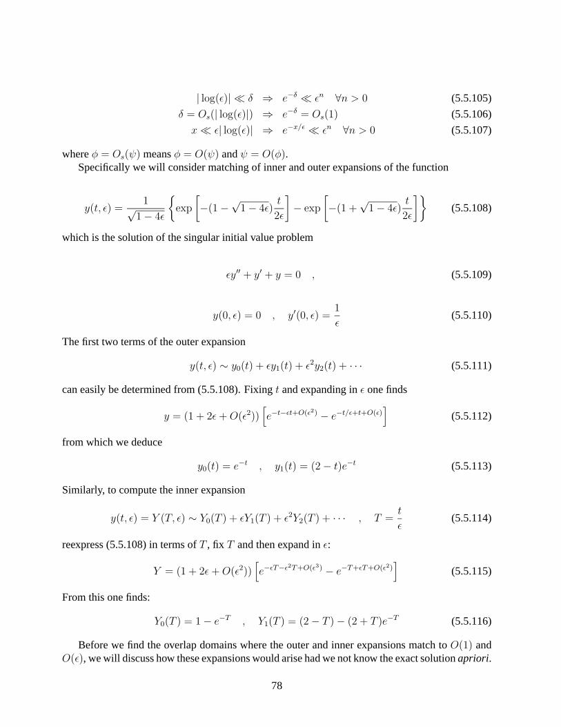
| log(ε)| δ ⇒ e−δ εn ∀n > 0 (5.5.105)

δ = Os(| log(ε)|) ⇒ e−δ = Os(1) (5.5.106)

x ε| log(ε)| ⇒ e−x/ε εn ∀n > 0 (5.5.107)

where φ = Os(ψ) means φ = O(ψ) and ψ = O(φ).Specifically we will consider matching of inner and outer expansions of the function

y(t, ε) =1√

1− 4ε

{exp

[−(1−

√1− 4ε)

t

2ε

]− exp

[−(1 +

√1− 4ε)

t

2ε

]}(5.5.108)

which is the solution of the singular initial value problem

εy′′ + y′ + y = 0 , (5.5.109)

y(0, ε) = 0 , y′(0, ε) =1

ε(5.5.110)

The first two terms of the outer expansion

y(t, ε) ∼ y0(t) + εy1(t) + ε2y2(t) + · · · (5.5.111)

can easily be determined from (5.5.108). Fixing t and expanding in ε one finds

y = (1 + 2ε+O(ε2))[e−t−εt+O(ε2) − e−t/ε+t+O(ε)

](5.5.112)

from which we deduce

y0(t) = e−t , y1(t) = (2− t)e−t (5.5.113)

Similarly, to compute the inner expansion

y(t, ε) = Y (T, ε) ∼ Y0(T ) + εY1(T ) + ε2Y2(T ) + · · · , T =t

ε(5.5.114)

reexpress (5.5.108) in terms of T , fix T and then expand in ε:

Y = (1 + 2ε+O(ε2))[e−εT−ε

2T+O(ε3) − e−T+εT+O(ε2)]

(5.5.115)

From this one finds:

Y0(T ) = 1− e−T , Y1(T ) = (2− T )− (2 + T )e−T (5.5.116)

Before we find the overlap domains where the outer and inner expansions match to O(1) andO(ε), we will discuss how these expansions would arise had we not know the exact solution apriori.

78

By substituting the expansion (5.5.111) into (5.5.109) we obtain the problems:

O(1) : y′0 + y0 = 0 (5.5.117)

O(ε) : y′1 + y1 = −y′′0 (5.5.118)

whose general solutions are (for a0, b0 constant)

y0(t) = a0e−t (5.5.119)

y1(t) = (b0 − a0t)e−t (5.5.120)

Clearly, a0 cannot be chosen so that y0(t) satisfy both initial conditions. Therefore, there must bea layer at t = 0. In terms of Y and T the initial value problem (5.5.109)-(5.5.110) can be written

Y ′′ + Y ′ + εY = 0 , (5.5.121)

Y (0, ε) = 0 , Y ′(0, ε) = 1 (5.5.122)

from which we obtain the inner problems

O(1) : Y ′′0 + Y ′0 = 0 , Y0(0) = 0 , Y ′0(0) = 1 (5.5.123)

O(ε) : Y ′′1 + Y ′1 = −Y0 , Y1(0) = 0 , Y ′1(0) = 0 (5.5.124)

whose solutions are that given in (5.5.116). In contrast to boundary value problems, the unknownconstants of integration to be determined from matching are part of the outer solution. If we applyPrandtl matching to match y0 and Y0 we find

limt→0+

y0(t) = a0 = 1 = limT→∞

Y0(T ) (5.5.125)

and recover y0(t) in (5.5.113).

Demonstrating extended outer domains to O(1)To find an extended domain for the outer expansion one assumes η(ε) 1 and seeks an η1(ε)

such that η1(ε) η(ε) implies

limε→0+,tη fixed

[y(ηtη, ε)− y0(ηtη)] = 0 (5.5.126)

for the intermediate variable

tη =t

η> 0 (5.5.127)

Given (5.5.112), this limit holds providing e−tηη/ε 1. To assure this, we choose η1(ε) =ε|log(ε)|. Now let the notation φ = ψ mean that either φ ψ or φ = Os(ψ). Then wecan conclude that Do will be an extended domain for the outer expansion so long as η satisfies

η1,0 ≡ ε|log(ε)| η = 1 (5.5.128)

79

Though each η defines a different region in the (x, ε)-plane for tη ∈ Iη, all that really matters forthe limit to vanish is that η satisfy (5.5.128). So it is common practice to say that the extendeddomain for the single term outer expansion y0(t). ”is” (5.5.128).

Demonstrating extended outer domains to O(ε)To find the extended domain for the two term outer expansion y0(t) + εy1(t) one assumes

η(ε) 1 and seeks an η1,1(ε) such that η1,1(ε) η(ε) implies

limε→0+,tη fixed

[y(ηtη, ε)− y0(ηtη)− εy1(ηtη)]ε

= 0 (5.5.129)

Again from (5.5.112), we find that if η satisfies (5.5.128) the above limit holds. That is to say thechoice η1,1 = η1,0 works. If we continue this process of extending the domain in an R term outerexpansion to find η1,R it is often the case that η1,R η1,R+1 since adding more terms to the limitplaces more restrictions on η. For this particular example the extended outer domains at O(1) andO(ε) turned out to be the same.

Demonstrating extended inner domains to O(1) and O(ε)To find an extended domain for the single term inner expansion one assumes ε η(ε) and

seeks an η2(ε) such that η η2(ε) implies

limε→0+,tη fixed

[y(ηtη, ε)− Y0(ηtη/ε)] = 0 (5.5.130)

Again from (5.5.112) it is easy to verify that the extended domain for the single term inner expan-sion is defined by

ε= η η2,0 ≡ 1 (5.5.131)

Finding the extended inner domain to O(ε) is more delicate. In terms of the intermediate variables

y(ηtη, ε)

ε=

1

ε− e

−tηη/ε

ε− ηεtη −

η

εtηe−tηη/ε + 2− 2e−tηη/ε

+O(η) +O

(η2

ε

)+O(ε)

and in terms of the intermediate variables

1

εY0 + Y1 =

y(ηtη, ε)

ε=

1

ε− e

−tηη/ε

ε− ηεtη −

η

εtηe−tηη/ε + 2− 2e−tηη/ε (5.5.132)

Subtracting these two expressions we see that

limε→0+,tη fixed

[y(ηtη, ε)− Y0(ηtη/ε)− εY1(ηtη/ε)]

ε= 0 (5.5.133)

provided η2/ε 1. That is to say the choice η2,1 = ε1/2 ensures the limit vanishes and theextended inner domain to O(ε) is

ε= η η2,1 ≡ ε1/2 (5.5.134)

80

Here we note the extended domain to O(ε) is ”smaller” than the domain to O(1), i.e. η2,1 η2,0.

Demonstrating overlap to O(1) and O(ε)Considering the previous discussions it is clear to see that the overlap domains to O(1) and

O(ε) are, respectively,

η1,0 η η2,0 (5.5.135)

η1,1 η η2,1 (5.5.136)

or

ε| log(ε)| η 1 (5.5.137)

ε| log(ε)| η ε1/2 (5.5.138)

If η satisfies these asymptotic relations, the outer and inner expansions match to O(1) and O(ε),respectively. Explicitly, if η satisfies (5.5.135) then

limε→0+,tη fixed

[y0(ηtη)− Y0(ηtη/ε)] = 0 (5.5.139)

And, if η satisfies the more stringent requirement (5.5.136)

limε→0+,tη fixed

[y0(ηtη) + εy1(ηtη)− Y0(ηtη/ε)− εY1(ηtη/ε)]

ε= 0 (5.5.140)

If the exact solution y was not known apriori then one would choose a0 in the incomplete outersolution y0(t) = a0e

−t and find η1,0, η2,0 so that (5.5.139) is satisfied.

1. Consider the problem

y′′ + εy′ + y = 0, y(0) = 1, y′(0) = 0. (*)

(a) Find the exact solution to this initial value problem.

(b) Obtain a two term regular asymptotic expansion for (*).

(c) Compare graphically your answer for ε = .25 and ε = .1 with the exact answer for0 ≤ x ≤ 2.

2. Obtain a two term regular expansion for y′′ + 2y = eεx, y(0) = y(1) = 0.

3. Obtain a two term regular expansion for (1 + εx2)y′′ + y = x2, y(0) = ε, y(1) = 1.

4. Find a two term expansion for y′′ = sin(x) y, y(0) = 1, y′(0) = 1 using the method ofsuccessive integration from Example 5.4.

5. Find a regular expansion for the system

{x = x− 2y + εxyy = x− 3y − εxy Is the expansion valid for all

t ≥ 0? Give a reason.

81

6. Use the method of strained variables to obtain a two term expansion for

(x+ εy)dy

dx+ y = 0, y(1) = 1.

Also find the exact solution and compare graphically your results and the exact solution onthe interval [0, 2] for ε = .1.

7. Use the method of averaging to find an approximate periodic solution to the Van der Poloscillator

y + y + ε(y2 − 1) y = 0,

i.e., find an approximation y(t) ∼ a(t) cos(t+ θ(t)), a(0) = a0, Θ(0) = Θ0.

8. Find a uniform asymptotic approximation to the boundary layer problem, i.e., find an inner,outer and matched solution.

εy′′ + (1 + ε)y′ + y = 0, y(0) = 0, y(1) = 1.

Also compute the exact solution and graphically compare your answers for ε = .1 andε = .025.

9. Find a uniform asymptotic approximation to the boundary layer problem, i.e., find an inner,outer and matched solution.

εy′′ + 2y′ + ey = 0, y(0) = 0, y(1) = 0

References

[1] C.M. Bender and S.A. Orzag, “Advanced Mathematical Methods for Scientists and Engi-neers, I,” Springer-Verlag, 1999.

[2] M.H. Holmes, “Introduction to Perturbation Methods,” Springer-Verlag, New York, 1995.

[3] E.L. Ince, “Ordinary Differential Equations,” Longman, Green and Co., London, 1927. Dover1956.

[4] J. Kevorkian and J.D. Cole, “Perturbation Methods in Applied mathematics,” Springer-Verlag, New York, 1981.

[5] J.D. Murray, “Asymptotic Analysis,” Springer-Verlag, Applied Math. Sciences Vol 48. 1984.

[6] A.H. Nafeh, “Perturbation Methods,” Wiley, New York, 1973.

[7] Frank Hoppensteadt, “Analysis and Simultion of chaotic Systems,” 2nd edition, Springer,2000.

[8] H. Keller “Numerical Methods for Two-Point Boundary Value Problems,” Blaisdell Pub. Co.,Waltham, Mass. (1968).

82

[9] J. Kevorkian and J.D. Cole, “Perturbation Methods in Applied mathematics,” Springer-Verlag, New York, 1981.

[10] J.D. Murray, “Asymptotic Analysis,” Springer-Verlag, Applied Math. Sciences Vol 48. 1984.

[11] A.H. Nafeh, “Perturbation Methods,” Wiley, New York, 1973.

[12] H. Sagan, “Boundary and Eigenvalue Problems in Mathematical Physics,” J. Wiley & Sons,Inc, New York, 1961.

[13] J.G. Simmonds and J.E. Mann, Jr., “A First Look at Perturbation theory,” second edition,Dover Publications, Inc. 1998.

[14] D.R. Smith, “Singular-Perturbation Theory,” Cambridge University Press, 1985.

[15] I. Stakgold, “Green’s Functions and Boundary Value Problems,” Wiley-Interscience, 1979.

[16] K. Yosida, “Lectures on Differential and Integral Equations,” Interscience Publishers, 1960.

83