5. EXPLANATORY NOTES
103
D’Hondt, S.L., Jørgensen, B.B., Miller, D.J., et al., 2003 Proceedings of the Ocean Drilling Program, Initial Reports Volume 201 5. EXPLANATORY NOTES 1 Shipboard Scientific Party 2 INTRODUCTION Information assembled in this chapter will help the reader under- stand the basis for our preliminary conclusions and will also enable the interested investigator to select samples for further analysis. This infor- mation concerns only shipboard operations and analyses described in the site reports in the Leg 201 Proceedings of the Ocean Drilling Program, Initial Reports volume. Methods used by various investigators for shore- based analyses of Leg 201 samples will be described in the individual contributions published in the Leg 201 Scientific Results volume and in publications in various professional journals. Authorship of Site Chapters The separate sections of the site chapters were written by the follow- ing shipboard scientists (authors are listed in alphabetical order, no se- niority is implied): Leg summary and principal results: Shipboard Scientific Party Background and objectives: D’Hondt, Jørgensen Operations: Miller, Storms Lithostratigraphy: Aiello, Meister, Naehr, Niitsuma Biogeochemistry: Blake, Dickens, Hinrichs, Holm, Jørgensen, Mit- terer, Solis Acosta, Spivack Microbiology: Cragg, Cypionka, Ferdelman, House, Inagaki, Jørgen- sen, Naranjo Padilla, Parkes, Schippers, Smith, Teske, Wiegel Physical properties: Bekins, Ford, Gettemy, Niitsuma, Skilbeck Downhole tools: Bekins, Dickens Downhole logging: Guèrin Observer (Ecuadorian): Naranjo Padilla Observer (Peruvian): Solis Acosta 1 Examples of how to reference the whole or part of this volume. 2 Shipboard Scientific Party addresses. Ms 201IR-105
Transcript of 5. EXPLANATORY NOTES

D’Hondt, S.L., Jørgensen, B.B., Miller, D.J., et al., 2003Proceedings of the Ocean Drilling Program, Initial Reports Volume 201
5. EXPLANATORY NOTES1
Shipboard Scientific Party2
INTRODUCTION
Information assembled in this chapter will help the reader under-stand the basis for our preliminary conclusions and will also enable theinterested investigator to select samples for further analysis. This infor-mation concerns only shipboard operations and analyses described inthe site reports in the Leg 201 Proceedings of the Ocean Drilling Program,Initial Reports volume. Methods used by various investigators for shore-based analyses of Leg 201 samples will be described in the individualcontributions published in the Leg 201 Scientific Results volume and inpublications in various professional journals.
Authorship of Site Chapters
The separate sections of the site chapters were written by the follow-ing shipboard scientists (authors are listed in alphabetical order, no se-niority is implied):
Leg summary and principal results: Shipboard Scientific PartyBackground and objectives: D’Hondt, JørgensenOperations: Miller, StormsLithostratigraphy: Aiello, Meister, Naehr, NiitsumaBiogeochemistry: Blake, Dickens, Hinrichs, Holm, Jørgensen, Mit-
terer, Solis Acosta, SpivackMicrobiology: Cragg, Cypionka, Ferdelman, House, Inagaki, Jørgen-
sen, Naranjo Padilla, Parkes, Schippers, Smith, Teske, WiegelPhysical properties: Bekins, Ford, Gettemy, Niitsuma, SkilbeckDownhole tools: Bekins, DickensDownhole logging: GuèrinObserver (Ecuadorian): Naranjo PadillaObserver (Peruvian): Solis Acosta
1Examples of how to reference the whole or part of this volume.2Shipboard Scientific Party addresses.
Ms 201IR-105

SHIPBOARD SCIENTIFIC PARTYCHAPTER 5, EXPLANATORY NOTES 2
Drilling Operations
Two standard coring systems were used during Leg 201, the advancedhydraulic piston corer (APC), and the extended core barrel (XCB). Thesestandard coring systems and their characteristics are summarized in the“Explanatory Notes” chapters of various previous Initial Reports volumesas well a number of Technical Notes. Most cored intervals were ~9.5 mlong, which is the length of a standard core barrel. In other cases thedrill string was drilled, or “washed ahead,” without recovering sedi-ments to advance the drill bit to a target depth where core recoveryneeded to resume.
Drilled intervals are referred to in meters below rig floor (mbrf),which are measured from the kelly bushing on the rig floor to the bot-tom of the drill pipe, and meters below seafloor (mbsf), which are calcu-lated from the length of pipe deployed less estimated seafloor depth.When sediments of substantial thickness cover the seafloor, the mbrfdepth of the seafloor is determined with a mudline core, assuming100% recovery for the cored interval in the first core. Water depth iscalculated by subtracting the distance from the rig floor to sea levelfrom the mudline measurement in mbrf. This water depth usually dif-fers from precision depth recorder measurements by a few to severalmeters. The mbsf depths of core tops are determined by subtracting theseafloor depth (mbrf) from the core top depth (mbrf). The resulting coretop datums in mbsf are the ultimate reference for any further depth cal-culation procedures.
Drilling Deformation
When cores are split, many show signs of significant sediment distur-bance, including the concave-downward appearance of originally hori-zontal bedding, haphazard mixing of lumps of different lithologies(mainly at the tops of cores), fluidization, and flow-in. Core deforma-tion may also occur during retrieval because of changes in pressure andtemperature as the core is raised and during cutting and core handlingon deck.
Curatorial Procedures and Sample Depth Calculations
Numbering of sites, holes, cores, and samples follows the standardOcean Drilling Program (ODP) procedure (Fig. F1). A full curatorialidentifier for a sample consists of the leg, site, hole, core number, coretype, section number, and interval in centimeters measured from thetop of the core section. For example, a sample identification of 201-1225A-1H-1, 10–12 cm, represents a sample removed from the intervalbetween 10 and 12 cm below the top of Section 1, Core 1 (H designatesthat this core was taken with the APC system) of Hole 1225A during Leg201. Cored intervals are also referred to in “curatorial” mbsf. The mbsfdepth of a sample is calculated by adding the depth of the sample be-low the section top and the lengths of all higher sections in the core tothe core top datum measured with the drill string.
A sediment core from less than a few hundred mbsf may, in somecases, expand upon recovery (typically 10% in the upper 300 mbsf),and its length may not necessarily match the drilled interval. In addi-tion, a coring gap is typically present between cores. Thus, a discrep-ancy may exist between the drilling mbsf and the curatorial mbsf. Forinstance, the curatorial mbsf of a sample taken from the bottom of a
sealevel
Core 201-1225A-2H Section 201-1225A-2H-5top
bottom of hole
void
Sample201-1225A-2H-5,80-85 cm
Hole 1225A
beacon
LEG 201SITE 1215
JOIDES Resolution
seafloor
water depth(m or mbsl)
penetration(mbsf)
Core Catcher (CC)
Section 3
Section 5
Section 4
Section 6
Section 1
Section 2
top (0 cm)
bottom(150 cm)
Core 1H80% recovery
Core 3R\H50% recovery
Core 2H90% recovery
F1. Coring and depth intervals, p. 67.

SHIPBOARD SCIENTIFIC PARTYCHAPTER 5, EXPLANATORY NOTES 3
core may be larger than that of a sample from the top of the subsequentcore, where the latter corresponds to the drilled core-top datum.
If a core has incomplete recovery, all cored material is assumed tooriginate from the top of the drilled interval as a continuous section forcuration purposes. The true depth interval within the cored interval isnot known. This should be considered as a sampling uncertainty in age-depth analysis and correlation of core facies with downhole log signals.
Core Handling and Analysis
To ensure as little damage as possible to the microbial communitiespresent in cores, a unique core processing strategy was established forLeg 201. Since microorganisms existing at deepwater seafloor tempera-tures (2°–4°C) can be acutely sensitive to elevated temperature (>10°C)and oxygen, we recognized a critical need to prevent thermal equilibra-tion and exposure of the cores to oxygen after recovery. To minimizeequilibration of the cores, we modified the standard coring practice ofshelving a recovered core barrel on the rig floor while a new core barrelis deployed and a joint of pipe is added. The core barrel was extractedfrom the drill string and immediately transferred to the catwalk andmarked by the ODP curatorial staff into 1.5-m sections. Shipboard mi-crobiologists identified one or more 1.5-m sections (hereafter referredto as the MBIO sections) for rapid microbiological processing. Once theMBIO sections were selected, they were labeled with a red permanentmarker with orientation and section number and removed from thecore. Ends of the removed sections were covered with plastic caps butnot sealed, and the sections were carried into the hold refrigerator,which was set to ~4°C and served as a microbiology cold room. Aftersome modifications to the cooling unit and installation of plastic sheetsacross the door to dampen air exchange, thermal loggers indicated anambient temperature in the cold room of ~6°C. Multiple sections weremoved to the cold room in order to ensure that sufficient undisturbedmaterial was available for microbiology and coupled geochemistry sam-pling. Microbiology and geochemistry samples were rapidly extracted,as described in “Whole-Round Core Sampling in the Cold Room,”p. 16, in “Core Handling and Sampling” in “Introduction and Back-ground” in “Microbiology.” Unsampled microbiological subsectionsand the remainder of the core on the catwalk were processed accordingto the ODP standard core handling procedures as described in previousInitial Reports volumes and the Shipboard Scientist’s Handbook (withminor modifications). In brief, prior to sectioning, an infrared (IR) cam-era was passed along the length of the core, capturing a thermally cali-brated image (see “Infrared Thermal Imaging,” p. 42, in “PhysicalProperties”). Routine shipboard safety and pollution prevention sam-ples were collected on the catwalk (see “Biogeochemistry,” p. 9). Thecore was then cut into nominally 1.5-m sections. The remaining cutsections were transferred to the core laboratory for further processing.
Whole-round core sections not used for microbiological samplingwere run through the multisensor track (MST), and thermal conductiv-ity measurements were performed (see “Physical Properties,” p. 41).The cores were then split into working and archive halves (from bottomto top); investigators should be aware that older material may havebeen transported upward on the split face of each section. When shortpieces of sedimentary rock were recovered, the individual pieces weresplit with the rock saw and placed in split liner compartments createdby sealing spacers into the liners with acetone.

SHIPBOARD SCIENTIFIC PARTYCHAPTER 5, EXPLANATORY NOTES 4
Coherent and reasonably long archive-half sections were measuredfor color reflectance using the archive-half multisensor track (AMST)(see “Color Reflectance Spectrophotometry,” p. 8, in “Lithostratigra-phy). Visual descriptions were prepared of the archive halves, aug-mented by smear slides and thin sections (see “Lithostratigraphy,”p. 4), and the archive halves were photographed with both black-and-white and color film. Close-up photographs were taken of particularfeatures for illustrations in site chapters, as requested by individual sci-entists. All sections of core not removed for microbiological samplingwere additionally imaged using a digital imaging track system equippedwith a line-scan camera.
The working half of each core was sampled for shipboard analysis,such as physical properties, carbonate, and bulk X-ray diffraction (XRD)mineralogy, and for shore-based studies. Both halves of the core werethen put into labeled plastic tubes, sealed, and placed in cold storagespace on board the ship. At the end of the leg, the cores were trans-ferred from the ship into refrigerated containers and shipped to theODP Gulf Coast Core Repository in College Station, Texas.
LITHOSTRATIGRAPHY
This section outlines the procedures followed to document the basiclithostratigraphy of the deposits recovered during Leg 201, includingcore description, XRD, color spectrophotometry, digital color imaging,and smear slide description. Only general procedures are outlined, ex-cept where they depart significantly from ODP conventions.
Age Assignments
All seven sites drilled during Leg 201 were located very close to sitesdrilled during previous cruises. The biostratigraphic and magnetostrati-graphic age framework presented in the site chapters follows those ofthe previous legs. The ages of biostratigraphic and magnetostratigraphicevents are those of Berggren et al. (1995a, 1995b).
Visual Core Descriptions
Information from macroscopic description of each core was recordedmanually for each core section on visual core description (VCD) forms.A wide variety of features that characterize the sediment were recorded,including lithology, sedimentary structures, color, and sediment defor-mation. Compositional data were obtained from smear slides. The color(hue and chroma) of the sediments was determined by color spectro-photometry (see “Color Reflectance Spectrophotometry,” p. 8). Thisinformation was condensed and entered into AppleCORE (version 8.1b)software, which generates a simplified one-page graphical descriptionof each core (barrel sheet) (Fig. F2). Barrel sheets are presented withsplit-core photographs (see the “Core Descriptions” contents list). Thelithologies of the recovered sediments are represented on barrel sheetsby symbols in the column titled “Graphic Lithology” (Fig. F3). Primarysedimentary structures, bioturbation parameters, soft-sediment defor-mation, structural features, and drilling disturbance are indicated incolumns to the right of the graphic log. The symbols are schematic butare placed as close as possible to their proper stratigraphic position. Forexact positions of sedimentary features, more detailed VCDs can be ob-
Site 1225 Hole A Core 23H Cored 205.3-214.8 mbsf
0.5
1.0
1.5
2.0
2.5
3.0
3.5
4.0
4.5
5.0
5.5
6.0
6.5
7.0
7.5
8.0
8.5
9.0
9.5
10.0
ME
TE
RS
12
34
56
78
SE
CT
ION
GR
AP
HIC
LIT
H.
STRUCTURE DIA
GE
NE
SIS
DIS
TU
RB
.
SS
PAL
SA
MP
LE
RADIOLARIAN-BEARING DIATOM-BEARING NANNOFOSSIL OOZE
Major Lithology:Light gray RADIOLARIAN-BEARING DIATOM-RICH NANNOFOSSIL OOZE
General Description:Pale green-yellow burrows are present in zones between diffuse pale green and purple laminated zones. Green cm-scaled bands and spots with opaque clasts (pyrite) occur sporadically in the sediment.
DESCRIPTION
F2. Example of a VCD form, p. 68.
Lithology
ContactsSharp ScouredUndulating Inclined
Structures
Fossils- Fish remains - Spicules
Diagenesis
Bioturbation
Drilling Disturbance
SamplesSS - Smear slide XRA - X-ray diffraction IW - Interstitial waterPPWR - Physical properties whole round PAL - Paleontology
- Bioturbation - minor - Bioturbation - moderate - Bioturbation - intense
- High-angle parallel bedding
- Low-angle parallel bedding
- Wavy parallel bedding
- Convolute bedding
- Planar lamination
- Color band
- Cross-bedding
- Normal-graded bedding
- Reverse-graded bedding
- Fining upward
- Slump
- Coarsening-upward
- Mottled
- Erosion surface - Sand lamina
- Silt lamina
- Microfault (normal)
- Thin ash layer
- Fault
- Macrofault (normal)
- Fluid escape structure
- Shell fragments
- Soupy
- Slightly disturbed
- Drilling breccia
- Very disturbed
Nannofossilooze
Foraminiferooze
Nannofossilchalk
Limestone
Dolomite
Void/No core
Whole-roundsample
Volcanic ashor tuff
Gravel
Metalliferoussediment
Sulfidesand
SulfidesiltSand
Siltysand
Clayeysand
Silt
Sandysilt
Chert
Clay
Clayeysilt
Siltyclay
Sandyclay
- Biscuit
- Moderately disturbed
- Dolomitic
- Pyrite
- Peloids
- Nodule/concretion, general
- Barite nodule/concretion
- Calcite nodule/concretion
- Calcedony/chert nodule/concretion
- Dolomite nodule concretion
- Pyrite nodule/concretion
- Cement, general
- Calcite cement
- Calcedony/chert cement
- Dolomite cement
- Carbonate nodule/concretionC
- Glauconite
- Phosphate
- Magnetite
- Calcareous
- Phosphate concretion
Gl
Fe
Ph
- Quartz cement
Ichnofossils
- Skolithos- Planolites - Zoophycos - Chondrites
Diatomooze
Diatomite
Porcellanite
Diatom-Rad.Ooze
Radiolarianooze
F3. Patterns and symbols used in barrel sheets, p. 69.

SHIPBOARD SCIENTIFIC PARTYCHAPTER 5, EXPLANATORY NOTES 5
tained from ODP. Deformation and disturbance of sediment resultingfrom the coring process are illustrated in the “Drilling Disturbance” col-umn. Blank regions indicate the absence of coring disturbance. Loca-tions of samples taken for shipboard analysis are indicated in the “Sam-ples” column. A summary lithologic description with sedimentologichighlights is given in the “Description” column of the barrel sheet. Thisdescription provides information about the major sediment lithologies,important minor lithologies, and an extended summary description ofthe sediments, including color, composition, sedimentary structures,trace fossils identified and extent of bioturbation, and other notablecharacteristics. Descriptions and locations of thin, interbedded, or mi-nor lithologies that could not be depicted in the “Graphic Lithology”column are also presented in “Description,” where space permits.
Lithologic Classification
The sediment classification scheme used during Leg 201 is descrip-tive and follows the ODP classification scheme (Mazullo et al., 1988),with some simplifying modifications for sediments that are mixtures ofsiliciclastic and biogenic components (Fig. F4). Classification is basedprimarily on macroscopic description of the cores and examination ofsmear slides. During Leg 201, the total calcium carbonate content of thesediments (see “Biogeochemistry,” p. 9) and XRD determined onboard were also used to aid in classification.
Composition and texture are the criteria used to define lithology.Textural names for the siliciclastic sediment components are derivedfrom the Udden-Wentworth (Wentworth, 1922) grain size scale (Fig.F5). The term clay is used only for particle size and is applied to bothclay minerals and other siliciclastic material <4 µm in size. Geneticterms such as pelagic, neritic, hemipelagic, and debris flow do not ap-pear in this classification.
The principal name applied to a sediment is determined by the com-ponent or group of components (e.g., total biogenic carbonate) thatcomprise(s) >60% of the sediment or rock, except for subequal mixturesof biogenic and siliciclastic material. The main principal names are asfollows.
Siliciclastic Sediments
If the total siliciclastic content is >60%, the main name is determinedby the relative proportions of sand, silt, and clay sizes when plotted ona modified Shepard (1954) classification diagram (Fig. F4A). Examplesof siliciclastic principal names are clay, silt, sand, silty clay, sandy clay,clayey silt, sandy silt, clayey sand, and silty sand.
Biogenic Sediments
If the total biogenic content is >60% (i.e., siliciclastic material <40%),then the principal name applied is ooze (Fig. F4B). Biogenic compo-nents are not described in textural terms. Thus, a sediment with 65%sand-sized foraminifers and 35% siliciclastic clay is called clay-rich fora-minifer ooze, not clay-rich foraminifer sand.
Mixed Sediments
In mixtures of biogenic and nonbiogenic material where the bio-genic content is 40%–60% (termed “mixed sediments” in the ODP clas-sification), the name consists of two parts: (1) a major modifier(s) con-sisting of the name(s) of the major fossil group(s), with the least
100755075
Sand100
100
7575
7575
50 50
Sand
Siltysand
Clayeysand
Sandysilt
Sandyclay
Clayeyclay
Siltyclay ClaySilt
Percent biogenic material
Nannofossilooze
Nanno-fossilclay
Nannofossil-rich clay
N.-
bear
ing
clay
Cla
y
Percent siliciclastic material
A
B
Silt Clay
100 95 90 60 40 0
0 5 10 40 60 100
F4. Classification of siliciclastic sediments, p. 70.
1/2
1/4
1/8
1/16
1/32
1/64
1/128
1/256
2.00
1.00
0.50
0.25
0.125
0.0625
0.0310
0.0156
0.0078
0.0039
-12.0
-8.0
-6.0
-2.0
-1.0
0.0
1.0
2.0
3.0
4.0
5.0
6.0
7.0
8.0
Gra
vel
San
dS
ilt
4096
256
64
4
Mud
Conglomerate/Breccia
Sandstone
Siltstone15.6
63
500
250
125
31
7.8
3.9
Boulder
Cobble
Pebble
Granule
Very coarse sand
Coarse sand
Medium sand
Fine sand
Very fine sand
Coarse silt
Medium silt
Fine silt
Very fine silt
0.00006 14.0 Claystone0.06 Clay
Millimeters (mm) Phi (φ) Wentworth size class Rock typeMicrometers (µm)
F5. Grain-size classification dia-gram, p. 71.

SHIPBOARD SCIENTIFIC PARTYCHAPTER 5, EXPLANATORY NOTES 6
common fossil listed first, followed by (2) the principal name appropri-ate for the siliciclastic components (e.g., foraminifer clay) (Fig. F4B).
If any component (biogenic or siliciclastic) represents between 10%and 40% of a sediment, it qualifies for minor modifier status and is hy-phenated with the suffix -rich (e.g., nannofossil-rich clay). When acomponent makes up only 5%–10% of the sediment, it can be indicatedwith a minor modifier that consists of the component name hyphen-ated with the word “bearing” (e.g. nannofossil-bearing clay). Wheretwo minor components are present, the most abundant accessory com-ponent appears closest to the principal name. Major and minor modifi-ers are listed in order of increasing abundance before the principalname.
Examples
15% foraminifers, 40% nannofossils, and 45% clay = foraminifer-richnannofossil clay,
5% diatoms, 10% radiolarians, and 85% clay = diatom- and radio-larian-bearing clay, and
10% diatoms, 35% silt, and 55% foraminifers = diatom-bearing silt-rich foraminifer ooze.
Induration
The following classes of induration or lithification were adopted andmodified from ODP Leg 188 (Shipboard Scientific Party, 2001). Theywere separated into three classes for biogenic sediments and two classesfor nonbiogenic sediments. For biogenic sediments and sedimentaryrocks, the three classes of induration are
Soft: sediment has little strength and is readily deformed under pres-sure of a finger or broad-blade spatula:
Ooze: unconsolidated calcareous and/or siliceous biogenic sedi-ment;
Firm: partly lithified sediments that are readily scratched with a fin-gernail or the edge of a spatula:
Chalk: semi-indurated biogenic sediment composed predomi-nantly of calcareous biogenic grains;
Diatomite: semi-indurated biogenic sediment composed predomi-nantly of diatoms; and
Radiolarite: semi-indurated biogenic sediment composed predomi-nantly of radiolarians;
Hard: well-lithified and cemented sediment that is resistant or impos-sible to scratch with a fingernail or the edge of a spatula:
Limestone: a white or gray indurated calcareous biogenic sediment;Porcelanite: a dull white porous indurated siliceous biogenic sedi-
ment; andChert: a lustrous conchoidal fractured indurated siliceous biogenic
sediment.
For nonbiogenic clastic sediments, the two classes of induration are
Soft: Gravel, sand, silt, clay; sediment core can be split with a wire cut-ter; and
SHIPBOARD SCIENTIFIC PARTYCHAPTER 5, EXPLANATORY NOTES 7
Hard: Conglomerate, sandstone, siltstone, claystone; cannot be com-pressed with finger pressure, or core must be cut with a band sawor diamond saw.
Special Rock Types
The definitions and nomenclatures of special rock types wereadopted and modified from ODP Legs 112 and 138 (Shipboard Scien-tific Party, 1988, 1992) and adhere as closely as possible to conventionalterminology. Three special rock types were especially important duringLeg 201: authigenic carbonates, phosphates, and metalliferous sedi-ments.
Carbonates and Phosphates
Authigenic minerals are indicated in the “Diagenesis” column of thecore description forms (barrel sheets). Carbonates (calcite and dolo-mite) are present as beds and nodules. In cases where it was possible toclearly identify the carbonate mineralogy, symbols for the respectivecarbonate minerals were used. The degree of lithification is noted in thecore description as friable where the rock showed only partly lithifica-tion or lithified where fully cemented. Phosphate-rich sediments werealso present, designated by a “Ph” in the “Lithologic Accessories” col-umn (distinct from “P,” which is commonly used during ODP legs todesignate pyrite). In accordance with the terminology used during Leg112, two different types of phosphatic materials are distinguished. F-phosphate is the designation given to friable, generally light-coloredlenses and layers of fine-grained carbonate fluorapatite (francolite). Theterm D-phosphate is used for those phosphatic peloids, nodules, grav-els, and phosphatic hardgrounds composed mainly of dense, hard,dark-colored francolite. The term “phosphorite” is restricted to layerscomposed mainly of phosphatic grains.
Metalliferous Sediments and Metal-Rich Oxides
Metalliferous sediments are composed of fine-grained granular sul-fides, oxides, and hydroxy oxides rich in iron and other transition ele-ments. They may be present near or within basement rocks in the sedi-mentary section or as dispersed grains as a minor component of othersediments. In the former instance, the metal-rich sediments may in-clude both primary precipitates and altered crystalline phases. Theymay also include X-ray amorphous semiopaque oxides. Metalliferoussediments are generally distinguished from other fine-grained nonbio-genic sediments on the basis of their chemistry (e.g., Fe [10 wt% on acarbonate-free basis]; [(Fe + Mn)/Ti] [25]). In the absence of such infor-mation at the time the cores were described, we distinguished this sedi-ment lithology on the basis of color, opaque mineral content of smearslides, and/or presence at the base of the sediment column.
Other metal-rich oxides, such as dispersed or nodular manganese ox-ides, are also present in equatorial Pacific sediments. They may bepresent near the sediment surface or may lie buried within the sedi-ment. They are distinguished by color, mineralogy, and, in the case ofnodules, by their physical appearance.
Smear Slide Analysis
Petrographic analysis of the sand- and silt-sized components of thesediment was primarily conducted by smear slide description. The

SHIPBOARD SCIENTIFIC PARTYCHAPTER 5, EXPLANATORY NOTES 8
slides were fixed by ultraviolet (UV) curing using Norland optical adhe-sive immersion medium. Alternatively, some of the slides were preparedwith heat cure medium. Tables summarizing data from smear slides areavailable (see “Smear Slides” for each site in the “Core Descriptions”contents list). These tables include information about the sample loca-tion, whether the sample represents a dominant (D) or a minor (M) li-thology in the core, and the estimated percentage ranges of sand, silt,and clay, together with all identified components. We emphasize herethat smear slide analysis provides only crude estimates of the relativeabundances of detrital constituents. The mineral identification of finer-grained particles can be difficult using only a petrographic microscope,and sand-sized grains tend to be underestimated because they cannotbe evenly incorporated into the smear. The presence of authigenic min-erals such as manganese oxides, pyrite, or carbonates was especiallynoted. The mineralogy of smear slide components was validated byXRD. The relative proportions of carbonate and noncarbonate materialsestimated from smear slides were validated by chemical analysis of thesediments (see “Biogeochemistry,” p. 9).
X-Ray Diffraction
XRD was used to support and verify the observations of the smearslide analysis to identify small-scale compositional changes, potentialauthigenic minerals, and to detect main silica phases. Each sample wasfreeze-dried, ground, and mounted with a random orientation into analuminum sample holder. For the measurements, a Philips PW-1729 X-ray diffractometer with a CuKα source (40 kV and 35 mA) and Ni filterwas used. Peak intensities were converted to values appropriate for afixed slit width. The goniometer scan was performed from 2° to 40°2θ ata scan rate of 1.2°/min (step = 0.01° and count time = 0.5 s). Diffracto-grams were peak-corrected to match the (100) quartz peak at 4.26 Å.Common minerals were identified based on their peak position and rel-ative intensities in the diffractogram using an interactive software pack-age (MacDiff version 4.1.1).
Color Reflectance Spectrophotometry
In addition to visual estimates of the color, reflectance of visible lightfrom soft sediment cores was routinely measured using a Minolta spec-trophotometer (model CM-2002) mounted on the AMST. The AMSTmeasures the archive half of each core section and provides a high-resolution stratigraphic record of color variations for visible wave-lengths (400–700 nm). Freshly split cores were covered with clear plas-tic wrap and placed on the AMST. Measurements were taken at 2.0-cmspacing. The AMST skips empty intervals and intervals where the coresurface is well below the level of the core liner but does not recognizerelatively small cracks or disturbed areas of core. Thus, AMST data maycontain spurious measurements that should, to the extent possible, beedited out of the data set before use. Each measurement recorded con-sists of 31 separate determinations of reflectance in 10-nm-wide spec-tral bands from 400 to 700 nm. Additional detailed information aboutmeasurement and interpretation of spectral data with the Minolta spec-trophotometer can be found in Balsam et al. (1997, 1998) and Balsamand Damuth (2000).

SHIPBOARD SCIENTIFIC PARTYCHAPTER 5, EXPLANATORY NOTES 9
Digital Color Imaging and Image Analysis
Systematic high-resolution line-scan digital images of the archive-half core were obtained using the GEOTEK X-Y digital imaging system(DIS). The DIS system was calibrated for black-and-white imagingapproximately every 12 hr.
After cores were visually described, they were placed in the DIS andscanned. A spacer holding a neutral gray color chip and a label identify-ing the section was placed at the base of each section and scannedalong with each core. Output from the DIS includes a Windows bitmap(.bmp) file and a Mr.Sid (.sid) file for each section scanned. The bitmapfile contains the original data with no compressional algorithms ap-plied, whereas the Mr.Sid files apply extensive compressional algo-rithms.
Additional postprocessing of data was done to achieve a medium-resolution JPEG image of each section and a composite JPEG image(stored as a Microsoft PowerPoint slide) of each core, which is compara-ble to the traditional photographic image of each core. The JPEG imageof each section was produced by an Adobe Photoshop batch job thatopened the bitmap file, resampled to a width of 0.6 in at a resolution of300 pixels/in, and saved the result as a maximum-resolution JPEG.
BIOGEOCHEMISTRY
Interstitial Water Samples
Shipboard interstitial water (IW) samples were obtained from 5- to30-cm-long whole-round intervals that were cut according to two gen-eral procedures. One set of IW intervals was cut on the catwalk, capped,and taken to the laboratory for immediate processing; the other set wascut from ends of shared microbiology cores that were subsampled inthe walk-in refrigerator, usually within an hour of removal from the cat-walk. During high-resolution sampling, when there were too many IWintervals to process immediately, the capped whole-round intervalswere stored temporarily in a freezer or refrigerator. Cores with high con-tents of hydrogen sulfide were processed and stored temporarily in afume hood.
After extrusion from the core liner, the surface of each whole-roundinterval was carefully scraped with a spatula to remove potential con-tamination. Sediments were then placed into a titanium squeezer, mod-ified after the standard stainless steel squeezer of Manheim and Sayles(1974). The piston was positioned on top of the squeezer, which wasthen flushed with nitrogen through the outlet for >2 min. Pressures ofup to 76 MPa were applied in the squeezer, calculated based on themeasured hydraulic press pressure and the ratio of the piston areas ofthe hydraulic press and the squeezer. Interstitial water was passedthrough a prewashed Whatman number 1 filter fitted above a titaniumscreen, filtered through a 0.45-µm Gelman polysulfone disposable filter,and subsequently extruded into a precleaned (10% HCl) 50-mL plasticsyringe attached to the bottom of the squeezer assembly. After collec-tion of interstitial water, the syringe was removed to dispense aliquotsfor shipboard and shore-based analyses.
A modification of the above procedure was implemented to preventloss of ephemeral constituents because of the backlog of interstitial wa-ter samples awaiting dispensing from the 50-mL syringes. In addition to

SHIPBOARD SCIENTIFIC PARTYCHAPTER 5, EXPLANATORY NOTES 10
the 50-mL syringe, IW samples were also collected in a 10-mL glasssyringe attached to the squeezer assembly and the 50-mL syringe via athree-way plastic valve. Interstitial water emerging from the disposablefilter at the bottom of the squeezer assembly was directed into one orthe other syringe as necessary for appropriate dispensing of aliquots.Use of the 10-mL syringe also avoided air bubbles and minimized con-tamination of this fraction of the interstitial water by dissolved O2.
Interstitial Water Analyses
Most IW samples were analyzed for routine shipboard measurementsaccording to standard procedures (Gieskes et al., 1991). Salinity wasmeasured as total dissolved solids using a Goldberg optical handheld re-fractometer. The pH was determined by ion-selective electrode. Alkalin-ity was determined by Gran titration with a Metrohm autotitrator.
A new procedure was implemented during Leg 201 to analyze for dis-solved inorganic carbon, employing a Coulometrics 5011 CO2 coulo-meter. An aliquot of 1.0 mL of interstitial water was pipetted into thereaction tube, followed by addition of 3.0 mL of 2-N HCl after attachingthe reaction tube to the coulometer apparatus. The liberated CO2 was ti-trated, and the end point was determined by a photodetector. Measuredconcentrations were corrected for the value of the acid blank. Analyti-cal uncertainty, based on repeated measurements of a sample of surfaceseawater, was ±1%.
Concentrations of chloride and sulfate were determined by manualdilution and manual injection into a Dionex DX-120 ion chromato-graph. Chloride concentrations were also determined at some sites bytitration with AgNO3. Quantification was based on comparison with In-ternational Association of the Physical Sciences of the Ocean (IAPSO)standard seawater.
Dissolved silica, phosphate, and ammonium concentrations were de-termined by spectrophotometric methods using a Shimadzu UV Mini1240 spectrophotometer. For phosphate analyses at Sites 1227–1229,the standard protocol was slightly modified. Previous analyses of dis-solved phosphate in interstitial waters of shallow Peru Margin sedi-ments at Site 684 and also Sites 680 and 681 were strongly affected bycolor interference because of high concentrations of hydrogen sulfide(Shipboard Scientific Party, 1988). At the Peru Margin Sites 1227, 1228,and 1229, we aimed to improve upon the standard ODP technique fordissolved phosphate analysis in H2S-rich IW samples. One approachwas to remove sulfide from the sample by acidification and degassing.Samples that had been titrated for alkalinity were used, as they are acid-ified and degassed. Furthermore, they are in a pH range appropriate forcolorimetric determination of phosphate by the phosphomolybdateblue method.
Selected trace metal concentrations were obtained using the Jobin-Yvon Ultrace inductively coupled plasma–atomic emission spectrome-ter (ICP-AES). Concentrations of boron, barium, iron, lithium, manga-nese, and strontium were determined following the procedures out-lined by Murray et al. (2000). Given the anticipated range of redoxenvironments at Leg 201 sites and the fact that many microbially medi-ated reactions depend on metal catalysts, IW samples were also exam-ined for a suite of redox-sensitive transition metals—copper, molybde-num, nickel, vanadium, and zinc. For these analyses, the shipboard“master” ICP-AES standard was modified so that concentrations of iron,

SHIPBOARD SCIENTIFIC PARTYCHAPTER 5, EXPLANATORY NOTES 11
manganese, lithium, boron, and strontium remained the same but withconcentrations of copper, molybdenum, nickel, vanadium, and zinc at200, 200, 200, 200, and 500 mM, respectively. Analytical standards forall elements were then prepared by analyzing mixtures of this masterstandard and seawater.
Dissolved sulfide (ΣH2S = H2S+HS–) was determined on 1-mL intersti-tial water samples injected into a pre-tared vial containing 0.5 mL of20% zinc acetate solution (20 g ZnAc/100 mL solution). Dissolved sul-fide was determined by the methylene blue method of Cline (1969) us-ing a Shimadzu UV Mini 1240 spectrophotometer and a Milton Roy Mr.Sipper sample introduction system. Iodometrically calibrated zinc sul-fide suspensions in zinc acetate solution were used to calibrate the di-amine reagent.
Nitrate and nitrite concentrations were determined spectrophoto-metrically on 1-mL samples according to the methods of Strickland andParsons (1972) using a Shimadzu UV Mini 1240 spectrophotometerwith a Milton Roy Mr. Sipper sample introduction system.
Volatile fatty acids (i.e., acetate and formate) were analyzed by ionexchange chromatography on a Dionex ion chromatograph equippedwith an anion exchange column (Dionex AS-15). Solutions of sodiumhydroxide and sulfuric acid were utilized as eluent and suppressant, re-spectively. A 1.0-mL sample of filtered interstitial water was slowly ap-plied to a sequence of ion exchange cartridges to remove interferingions (cartridge A: Dionex OnGuard II H packed with a Ag-form cationicresin to remove chloride followed by cartridge B: Dionex OnGuard II Hpacked with a proton-form cationic resin to remove excess Ag elutingfrom previous cartridge) and after a period of at least 5 min eluted with1.0 mL H2O. Prior to use, cartridges were conditioned by rigorous flush-ing with deionized water (at least 20 mL). The detection limit for ace-tate was constrained by interferences with variable amounts of lactateand typically ranged from 0.2 to 0.5 µM. The detection limit for for-mate was 0.1 µM.
Gas Analyses
Hydrogen concentrations were determined on incubated sedimentsamples following published procedures that assume the headspace hy-drogen is in equilibrium with the dissolved pore fluid hydrogen (Lovleyand Goodwin, 1987; Hoehler et al., 1998). Four replicate incubationswere conducted on each sample. For each incubation, a 5-cm3 bulk sed-iment sample was collected from a freshly exposed end of a core sectionusing a sterilized plastic syringe with its Luer tip cut off. The sedimentsample was extruded into a 20-mL headspace vial and immediatelycapped with a rubber septum that was sealed with an aluminum crimpcap. The sealed vials were flushed with low-hydrogen nitrogen usingtwo hypodermic needles inserted through the septum. One needle wasconnected to the nitrogen and one allowed for gas release. These septaand vials were previously shown not to leak significant hydrogen overthe timescale of the incubations. Headspace hydrogen concentrationswere analyzed daily until approximately steady-state concentrationswere reached. Hydrogen concentrations were determined by gas chro-matography on a Trace Analytical reduction gas analyzer. Quantifica-tion was by comparison to a standard curve generated from a single pri-mary gas standard and mixed to different concentrations immediatelyprior to analysis. To correct for drift, the primary gas standard was re-
SHIPBOARD SCIENTIFIC PARTYCHAPTER 5, EXPLANATORY NOTES 12
peatedly analyzed. Reported concentrations are based on the tempera-ture-dependent solubility of hydrogen and the mean of replicates.
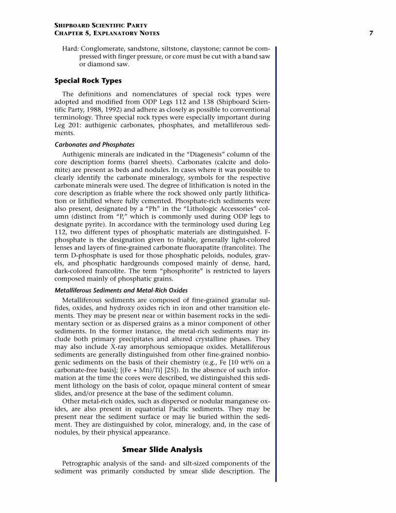
Concentrations of methane were monitored at intervals of 2 to 17samples per core. The standard gas analysis program for safety and pol-lution prevention purposes (Kvenvolden and McDonald, 1986) wascomplemented by additional headspace analyses following a slightlydifferent approach (Iversen and Jørgensen, 1985; Hoehler et al., 2000)with the intent to better constrain the concentrations of dissolvedgases. Compared to the rapid safety-oriented protocol, the latter, moretime-consuming alternative led to higher yields of methane (e.g., see“Biogeochemistry,” p. 14, in the “Site 1225” chapter).
Upon core retrieval, a 3-mL sediment sample was collected with acut-off plastic syringe from a freshly exposed end of a core section andwas extruded into a 20-mL glass serum vial. For this purpose, theplunger was held at the sediment surface while inserting the barrel toavoid trapping air bubbles. After withdrawing the syringe, the plungerwas advanced slightly to extrude a small amount of sediment. This ex-cess was shaved off with a flat spatula flush with the end of the syringebarrel to provide an accurate determination of the sediment volumewithin the syringe. Samples required for safety and pollution preven-tion purposes were immediately sealed with a septum and metal crimpcap and heated to 60°C for 20 min. The headspace was subsequentlyanalyzed by gas chromatography. For samples designated for refinedheadspace analysis, the sediment was extruded into a 20-mL vial con-taining 5 mL of 1-M NaOH. The vial was immediately capped with a sil-icone/Teflon septum. After vigorous manual shaking for 2 min, thevials were shaken automatically for an additional hour and subse-quently left to stand for at least 23 hr at room temperature prior to gaschromatographic analysis. Additionally, when gas pockets were ob-served, headspace samples were complemented by vacutainer samples,which were collected directly from gas voids formed in the core liner bypenetrating the liner using a syringe connected to a penetration tool.
Gas chromatographic analyses of headspace samples resulting fromboth protocols were performed in an identical manner. A 5-mL volumeof headspace gas was extracted from the vial using a standard gas sy-ringe. This volume was compressed in the syringe to a volume of 3 mL.The created overpressure was released by briefly opening the valve ofthe gas-tight syringe. Constituents of the headspace and vacutainer gassamples were analyzed using a Hewlett Packard 6890 Plus gas chro-matograph (GC) equipped with an 8-ft × 1/8-in stainless steel columnpacked with HaySep S (100–120 mesh) and a flame ionization detector(FID). Concentrations of methane, ethane, ethene, propane, and pro-pene were obtained. The carrier gas was helium, and the GC oven wasprogrammed from 100°C (5-min hold) to 140°C (4.5-min hold) at a rateof 50°C/min. Data were collected using a Hewlett-Packard 3365 Chem-Station data processing program. Gas samples collected with vacutain-ers were routinely analyzed on the natural gas analyzer (NGA). TheNGA system consists of a Hewlett-Packard 6890 Plus GC equipped withthree different columns and two detectors. Hydrocarbons from meth-ane to hexane were analyzed using a 60-m × 0.32-mm DB-1 capillarycolumn connected to a FID. The GC oven was heated isothermally at50°C for 15 min.
The concentration of methane in interstitial water was derived fromthe headspace concentration by the following equation:
CH4 = χM · Patm · VH · R–1 · T–1 · φ –1 · VS–1, (1)

SHIPBOARD SCIENTIFIC PARTYCHAPTER 5, EXPLANATORY NOTES 13
where,
VH = volume of the sample vial headspace,VS = volume of the whole sediment sample,χM = molar fraction of methane in the headspace gas (obtained from
GC analysis),Patm = pressure in the vial headspace (assumed to be the measured at-
mospheric pressure when the vials were sealed),R = the universal gas constant,T = temperature of the vial headspace in degrees Kelvin, andφ = sediment porosity (determined either from moisture and den-
sity measurements on adjacent samples or from porosity esti-mates derived from gamma ray attenuation [GRA] datarepresentative of the sampled interval).
Quantities of methane that remain undetected because of dissolutionin the aqueous phase are minimal (e.g., Duan et al., 1992) and are notaccounted for. The internal volumes of 15 representative headspace vialswere carefully measured beforehand and were determined to average18.42 ± 0.13 mL. This volume was taken as constant in calculations ofgas concentrations.
During Leg 201, we discovered that at most sites the concentrationsobtained from the safety-related headspace protocol were significantlylower than those obtained from comparable samples analyzed by theprolonged extraction method using sediment slurries in NaOH solu-tion. We suggest that the prolonged extraction solution led to the de-tection of a methane fraction that is not dissolved in interstitial water.For Sites 1229–1231, where particularly long extraction times had beenapplied and led to unusually high-yield increases, we consider the dataobtained from the safety protocol as the best approximation for thefraction of dissolved methane. Future research will verify the nature ofthe additional pool of methane tapped by prolonged extraction in alka-line solution.
Sediments
Sediment samples were not routinely analyzed during Leg 201 be-cause of the emphasis on interstitial water and gas analyses and becauseall of the sites drilled during this leg were sampled during previous legs.However, some analyses were obtained on sediment samples accordingto the standard methodology employed during previous legs. Inorganiccarbon (IC) concentration was determined using a Coulometrics 5011CO2 coulometer. About 10 to 15 mg of freeze-dried, ground sedimentwas weighed and reacted with 2-N HCl. The liberated CO2 was titrated,and the end point was determined by a photodetector. Calcium carbon-ate, expressed as weight percent, was calculated from the IC content, as-suming that all evolved CO2 was derived from dissolution of CaCO3, bythe following equation:
CaCO3 (wt%) = 8.33 × IC (wt%). (2)
No correction was made for the presence of other carbonate minerals.Total carbon (TC), nitrogen, and sulfur concentrations were deter-
mined using a Carlo Erba 1500 CNS elemental analyzer. About 10 mg offreeze-dried, ground sediment was weighed and combusted at 1000°C

SHIPBOARD SCIENTIFIC PARTYCHAPTER 5, EXPLANATORY NOTES 14
in a stream of oxygen. Nitrogen oxides were reduced to nitrogen, andthe mixture of carbon dioxide, nitrogen, and sulfur dioxide was sepa-rated by GC and detected by thermal conductivity detector (TCD). Totalorganic carbon (TOC) concentration was calculated as the differencebetween TC and IC concentrations.
The organic matter in selected sediment samples was characterizedby pyrolysis using a Delsi Nermag Rock-Eval II system. This method isbased on a whole-rock pyrolysis technique designed to characterize thetype and maturity of organic matter and to estimate the petroleum po-tential of the sediments (Espitalié et al., 1986). The Rock-Eval system in-corporates a temperature program that initially expels volatile hydro-carbons (S1) as the sample is heated at 300°C for 3 min and then, as thetemperature increases from 300° to 600°C at 25°C/min, releases the hy-drocarbons (S2) resulting from thermal cracking of kerogen. S1 and S2
hydrocarbons are measured and reported in milligrams per gram of drysediment. The temperature at which the kerogen yields the maximumamount of hydrocarbons during the S2 program provides Tmax, a param-eter used to assess the maturity of the organic matter. Between 300° and390°C of the pyrolysis program, carbon dioxide (S3) is released from theorganic matter, trapped, measured by TCD, and reported in milligramsper gram of dry sediment. Rock-Eval II parameters are used to character-ize organic matter by calculation of hydrogen index (HI), oxygen index(OI), and S2/S3:
HI = (S2/TOC) × 100 and (3)
OI = (S3/TOC) × 100. (4)
Rock-Eval data are generally unreliable for samples containing <0.5wt% TOC.
MICROBIOLOGY
Introduction and Background
ODP’s recent progress in exploring the deep subseafloor biospherehas revealed that prokaryotes are consistently present in core samplesrecovered from the deep oceanic subsurface (Parkes et al., 1994; Wells-bury et al., 1997). The subseafloor biosphere has been estimated to con-stitute one-third of the biomass on Earth (Whitman et al., 1998). How-ever, the structure, diversity, and function of subsurface microbialcommunities remain poorly understood. Total cell numbers alone donot provide information about prokaryotic physiologies that are criticalto understanding deep biosphere biogeochemical processes. It is impor-tant to know (1) what types of prokaryotes are present and in whatabundance and (2) which of these prokaroytes are truly active (i.e., notdormant) and are participating in deep sedimentary geochemical pro-cesses. We used a range of approaches to quantify prokaryote abun-dance, diversity, and activity, including (1) total counts; (2) adenosinetriphosphate (ATP); (3) cultivation methods, particularly the most prob-able number (MPN) technique; (4) nucleic acid–based techniques, par-ticularly fluorescence in situ hybridization (FISH); and (5) radiotracerand stable isotope tracer experiments on specific microbial processes. Inorder to ensure that we were indeed analyzing the indigenous prokary-

SHIPBOARD SCIENTIFIC PARTYCHAPTER 5, EXPLANATORY NOTES 15
otes and their activities, tests for contamination were conducted duringthe entire coring process for microbiological samples.
Core Handling and Sampling
Drilling
Microbiological sampling depends on careful and appropriate samplehandling technique. Precise operational definitions for special microbi-ology handling terminology is given in Table T1. Because the sampleswere retrieved from very stable sedimentary environments, the prokary-otes are expected to be sensitive to chemical and physical change, inparticular to changes in oxygen, temperature, and (for the deep-seasites) pressure. Consequently, all samples for microbiology and processstudies were transferred from the drilling platform to the hold refrigera-tor (set to <10°C) as quickly as possible and were kept as whole-coresections until processed (to date, there is no system for retrieving andmaintaining samples under in situ pressure). In order to avoid intermit-tent warming of retrieved cores, ODP’s usual core handling procedurewas modified. Once a core was retrieved, it was immediately transferredto the catwalk for labeling and cutting before the next core barrel wasdeployed. When piston coring at 3800 m water depth, this prolongedthe drilling operation by 33% per core (from 63 to 84 min) but was con-sidered important to prevent damage to heat-sensitive microorganisms.Efforts were also made to obtain APC cores even when this led to an in-crease in core recovery times, as APC cores were generally much less dis-turbed than XCB cores.
While drilling cores for microbiology, the potential for contamina-tion with bacteria from the surface is highly critical. Contaminationtests were continuously conducted using solutes (perfluorocarbontracer [PFT]) or bacterial-sized particles (fluorescent microspheres) tocheck for the potential intrusion of drill water from the periphery to-ward the center of cores and thus to confirm the suitability of the corematerial for microbiological research. We used the chemical and parti-cle tracer techniques described in ODP Technical Note 28 (Smith et al.,2000a). Furthermore, the freshly collected cores were visually examinedfor possible cracks and other signs of disturbance by observationthrough the transparent core liner. Core sections observed to be dis-turbed before or after subsampling were not analyzed further. Such dis-turbance phenomena are critical to the integrity of the core materialand therefore also to its usefulness for microbiological studies.
Sampling on the Catwalk
A limited number of microbiological and related biogeochemicalsamples were collected on the catwalk as soon as the core was retrieved.After the core was cleaned and the IR camera scan completed, the corewas marked into 1.5-m sections for cutting and visually inspected forsigns of disturbance, such as gas voids, cracks, and drilling disturbance.The appropriate sections, usually from the middle, were taken for mi-crobiological analyses. The top end of the selected sections were cutand capped (without acetone). The top 15 cm of this section (or thebottom 15 cm of the previous section) was often used as an interstitialwater biogeochemistry sample. The lower end was cut, and a tempera-ture image was immediately taken by a calibrated IR-sensitive videocamera (see “Infrared Thermal Imaging,” p. 42, in “Physical Proper-ties”) to estimate the maximum temperature reached in the core centerbefore it was transferred to the cold room. Samples for total prokaryotic
T1. MBIO sampling terms, p. 81.

SHIPBOARD SCIENTIFIC PARTYCHAPTER 5, EXPLANATORY NOTES 16
cell counts and perfluorocarbon contamination checks were immedi-ately collected using 5-cm3 sterile syringes from the lower, freshly cutend, whereas samples for methane and porosity were taken from theadjacent core section end. This catwalk syringe sampling enabled col-lection of these samples at a much greater frequency than was possiblefor the whole-round cores (WRCs). The lower core end was then sealedwith an end cap (without acetone). The microbiological section and anadjacent section were quickly transported to the cold room to limittemperature increase (see “Infrared Scanner,” p. 24, in “Physical Prop-erties,” in the “Site 1225” chapter).
Whole-Round Core Sampling in the Cold Room
It is important to emphasize that the different analyses, experiments,and cultivation attempts that fall under the rubric “microbiologicalmethods” have widely different requirements concerning handling andstorage. Keeping samples cool, processing times short, and minimizingcontamination were the key criteria for determining how the core sec-tions were processed. To minimize changes in the microbial population,all handling took place in a cold room. The lower refrigerated coreroom on the hold deck of the ship served as a cold room at <10°C andwas equipped with a work bench and working space for two to four per-sons. It was important that all materials, including core cutters, glassvials, and so on, were kept cold so that no unintentional warming ofthe samples took place. In addition, as the core liner is not sterile andthe outer surface of the core is contaminated during drilling (Smith etal., 2000a, 2000b), subsampling must exclude the sediment next to thecore liner. Where appropriate, handling and subsampling were per-formed under anoxic conditions.
Normally, two 1.5-m core sections at a time were brought down tothe cold room in case the standard section or a part of this section wasfound to be disturbed on subsampling. In such cases, part or all of thesubsequent section was also subsampled. Table T2 and Figure F6 showthe various categories of samples and how they were handled. The sub-sectioning equipment included the standard ODP core cutter coupledwith a clean wire or blade and a nitrogen-flushed cutting rig that wasmodified from an earlier published version (Fig. F7) (Parkes et al.,1995). The cutting rig system enabled a 1.5-m section, after cleaningthe outer surface with ethanol, to be sequentially cut into a number ofWRC sections using a sterile blade. Some of these WRC sections wereimmediately capped with clean end caps and stored at 4°C for shore-based analysis, whereas others were immediately subsampled into ster-ile 5-cm3 or larger syringes (with the Luer end removed).
To minimize contamination and to increase handling efficiency, sev-eral modifications of the core cutting procedure were introduced formicrobiology subsamples intended for cultivation, starting from Site1226. These include the following:
1. Replacing sterile cutting blades with a sterile cutting wire to min-imize the surface area that can draw contamination from theouter or inner core liner surface into the center portion of thecore;
2. Taking slurry samples using a large syringe that is centered on acore section instead of using several smaller syringes that, if notproperly centered, more easily pick up contamination from theouter core layers (the many smaller syringes that had been used
T2. Sampling codes and packing types, p. 82.
Sections 3 and 4 cut on catwalk
AODC,CH4,PFC
RemainingWRC(x cm)
FISH(6 cm)
TurnoverH2, SO4,
MagneticsCHNS(6 cm)
FeS(5 cm)
Biomarkers(X x 5-10 cm)
DNA(X x 5 cm)
ATP(10 cm)
IW(15 cm)
Clean, anoxic cutting Clean cutting
Both sections transferred to cold room; unused portion of Section 4 returned to curation path
RemainingWRC(x cm)
TurnoverH2, SO4,
MagneticsCHNS(6 cm)
Clean, anoxic cutting Clean cutting
AOM(5 cm)
13C intobiomarkers
(10 cm)
TurnoverAc, Bi, Thy,
H3, PO4, 18O(12 cm)
DIFF(5 cm)
Cells(5 cm)
FeS(6 cm)
Biomarkers(X x 5-10 cm)
DNA(X x 5 cm)
ATP(5 cm)
Slurries, MPN,enrichments,
FISH, AODC, 13C,contamination
(14 cm)
IW(15 cm)
Clean cutting
AODC,CH4,PFC
1 6 75432
3 4
Routine subsampling of Section 3
Expanded subsampling of Sections 3 and 4
ODP catwalk cut ODP catwalk cut ODP catwalk cut
Sterile break
FISH(6 cm)
SRR(5 cm)
F6. Diagram of WRC sectioning for MBIO, p. 72.
F7. N2-gassed cutting rig for WRCs, p. 73.

SHIPBOARD SCIENTIFIC PARTYCHAPTER 5, EXPLANATORY NOTES 17
for the initial slurry subsampling on Cores 201-1225A-2H and12H may have contributed to contamination); and
3. Obtaining an uncontaminated sediment surface by breaking thecore after precutting the core liner (however, in a Site 1225 test,depending on its texture and lamination a core tended to breakat irregular points and angles or even at more positions, thus en-hancing the air exposure of the samples).
After Site 1225, the nitrogen-flushed cutting rig was used principallyfor samples requiring anoxic sampling conditions (e.g., activity measure-ments).
Anoxic subsampling with cut-off syringes was conducted under aflow of filter-sterilized nitrogen in a gassing “bucket” designed at BristolUniversity (Fig. F8). The bucket system prevents the nitrogen flow fromcreating turbulence and thus introducing contamination or oxygen. Sy-ringe subcores were taken from the central uncontaminated part of theWRC and then sealed under nitrogen with a sterile stopper. To preservethe integrity of the sample during subcoring and to prevent sedimentnear the core liner from being sampled, sterile acrylic pegs were insertedinto the holes left after each subcore was removed. Subcores were storedat 10°C under nitrogen atmosphere in gas-tight bags until further pro-cessing. In compacted sediments, it was occasionally necessary to drivethe syringe into the WRC with a syringe adapter and hammer. Syringesubcores were used for various analyses, including radiotracer studies,production of sediment slurries for bacterial enrichments, MPN counts,FISH, bead contamination tests, and measurements of hydrogen con-centration.
WRCs to be immediately preserved were sectioned with a standardODP cutter and sterile wire from the same core. The samples fordeoxyribonucleic acid (DNA) and lipid biomarker analysis were frozenin a –80°C freezer. Samples for iron, manganese, and sulfur solid-phasespeciation and isotopes were placed in aluminum gas-tight bags,vacuum sealed, and frozen at –20°C. WRCs for further shore-basedmicrobiological experimentation were stored in a nitrogen gas–flushedaluminum bag, often together with a welled Merck Anaerocult strip,and stored at +4°C. Clean disposable gloves were worn during all han-dling procedures. Any remaining portions of the sections used for mi-crobiology subsampling were returned to the core laboratory for rein-troduction into the standard core handling process. In order to obtainuncontaminated material for slurry preparation and cultivation, coreswere broken after precutting the core liner with the ODP cutter. Bend-ing the outer ends upward allowed released particles to drop into a bin.This technique provided untouched (although not always smooth) sur-faces that were sampled by a 60-mL syringe. Only deeper sediment con-tents of the syringe, which did not contain oxygen, were transferred tonitrogen-flushed sterile slurry vessels containing artificial seawater. Anoverview of the cutting and subsampling scheme for the microbiologysection is given in Figure F6 and in Table T2.
Total Cell Counts and Contamination Tests
The most immediate method to visualize and quantify the deep bio-sphere are total prokaryotic cell counts using the nucleic acid stain acri-dine orange. These counts have been made on a wide range of ODP sed-iment cores, including cores from the Peru margin and the equatorialPacific (Parkes et al., 1994). In general, these counts have demonstrated
F8. Bucket for clean anoxic sub-sampling of WRCs, p. 74.

SHIPBOARD SCIENTIFIC PARTYCHAPTER 5, EXPLANATORY NOTES 18
an exponential decrease of prokaryotic cells with depth. Prokaryoticcells were consistently detected, even in the deepest sediments. Themethod detects sediment layers of increased cell density that often co-incide with particular geochemical conditions that are conducive toprokaryote growth (Parkes et al., 2000). The acridine orange directcount (AODC) enumeration method was used at all sites during this leg.Contamination during drilling and handling was evaluated by tests us-ing micrometer-sized fluorescent beads and PFT. These tests have shownthat core samples can be obtained without introducing prokaryotic cellcontamination, which is essential for almost all microbiological analy-ses that follow core retrieval (Smith et al., 2000a, 2000b).
Adenosine Triphosphate Analysis
WRCs were cut in the cold room and stored at –80°C for shore-basedanalysis of ATP concentrations using the luciferin-luciferase assay.Adenosine-5′-triphosphate is used as a common currency of energy forall organisms on Earth. ATP is generated by energy-yielding reactionsand is subsequently consumed in energy-requiring reactions in the cell.Because ATP molecules degrade rapidly upon cell death, ATP concentra-tions can be used as an indicator of total living biomass (Levin et al.,1964). This approach has been used in various marine environments(Holm-Hanson and Booth, 1966), including sediments (Karl andLaRock, 1975; Stoeck and Duineveld, 2000). ATP will be extracted fromsediments and quantified using the luciferin-luciferase assay. These datawill be compared to total cell counts in order to estimate the fraction ofthe observed community that is viable.
Cultivation Techniques
Using classic cultivation techniques such as the MPN cultivationmethod, various physiological types of prokaryotes have been enrichedfrom deep sediments and their abundances determined (e.g., Parkes etal., 2000). The MPN method allows quantification of the number ofviable prokaryotes according to a statistical evaluation of the number oftubes of different tenfold dilutions in which growth has been detected(Garthright, 2001). The prokaryotic types that have been cultured fromsediment ODP obtained using the MPN method include aerobic am-monifiers, nitrate reducers, fermentative anaerobic heterotrophs, sul-fate reducers, methanogens, acetogens, and anaerobic hexadecane oxi-dizers (Cragg et al., 1990, 1996; Bale et al., 1997; Barnes et al., 1998;Parkes et al., 2000; Wellsbury et al., 2000). MPN population countsrange from 0 to 105 cells/cm3 and generally decrease with increasingdepth. By MPN enumeration, however, generally far fewer than 0.6% ofthe total cell numbers in deep sediments are detected, and these viablecounts thus yield only limited quantitative information about the mi-crobiology of the deep subsurface. In surface sediments, higher MPNcounts have been obtained by the use of complex low-substrate mediaprepared from sediment extracts and containing fine particles (Vesterand Ingvorsen, 1998). Such an approach was used during Leg 201 forthe first time with deep sediments.
Cultivation is the only way to obtain microorganisms and studytheir physiology in order to estimate their impact on biogeochemicalcycles in deep sediments. For this reason, we enriched (with the aim toisolate and characterize) various types of microorganisms using a widerange of media and culture conditions that covered a wide range of en-

SHIPBOARD SCIENTIFIC PARTYCHAPTER 5, EXPLANATORY NOTES 19
vironmental conditions and metabolic requirements. Without goinginto detail about the media, which are listed in “Enrichments Near InSitu Temperatures,” p. 29, in “Methods for Enrichment and MPN” in“Procedures and Protocols,” the following groups of prokaryotes weretargeted:
1. Psychrophiles and mesophiles. Because the deep subsurface sed-iments drilled during Leg 201 are generally cold, many incuba-tions were kept at low temperatures of 4°–15°C in order to obtaincold-adapted (psychrophilic) prokaryotes that are characteristicof permanently cold sediments (Knoblauch et al., 1999a, 1999b;Knoblauch and Jørgensen, 1999).
2. Thermophiles. As microbial surveys of cold near-surface sedi-ments have in several cases detected thermophilic microorgan-isms (Isaksen and Jørgensen, 1994; Inagaki et al., 2001) thatpresumably represent dispersed microorganisms from other en-vironments or remnant populations of former high-temperatureenvironmental regimes, thermophiles, extreme thermophiles,and hyperthermophiles were also enriched during Leg 201.
3. Anaerobic prokaryotes. Because anaerobic processes (sulfate re-duction, metal reduction, fermentation, acetogenesis, and me-thanogenesis) are assumed to be the most relevant microbialprocesses in deeply buried sediments, media were almost exclu-sively geared toward enrichment of anaerobic prokaryotes(Balch et al., 1879; Widdel and Bak, 1992; Lovley and Phillips,1986, 1988; Thamdrup et al., 2000).
4. Oligotrophic prokaryotes. Whereas some bacteria may be iso-lated from marine sediments on media rich in acetate, lactate,and so on, others may not be able to cope with high concentra-tions of low molecular weight substrates in synthetic media.Microorganisms in nature have available complex organic sub-strates in small concentrations. Therefore, media that containnatural sterilized organic sediment extract or complex mixturesof recalcitrant substrates were included in the survey.
5. Chemolithotrophic bacteria. Organic carbon availability is gen-erally a dominant factor in shaping prokaryote community com-position and density. However, many microorganisms have achemolithotrophic energy metabolism, which means that theyutilize inorganic electron donors. Potential electron donors in-clude ammonium, hydrogen sulfide, elemental sulfur, hydro-gen, iron(II), manganese(II), or methane. Electron acceptors maybe oxygen, nitrate, iron(III), manganese(IV), sulfate, or carbondioxide. The media used during Leg 201 included combinationsof such inorganic electron donors and acceptors.
Microbial Molecular Analysis
Culture-independent molecular ecological surveys are becoming anindispensable and powerful approach to investigating naturally occur-ring microbial diversity. Molecular community analysis of deep subsur-face microbial ecosystems also offers new ways to understand the rela-tionship between microbial community composition, microbialactivities, and the biogeochemical characteristics of the sedimentarymicrobial biosphere (Sahm et al., 1999; Madson, 2000; Marchesi et al.,2001). Multiple molecular analytical techniques were applied to the

SHIPBOARD SCIENTIFIC PARTYCHAPTER 5, EXPLANATORY NOTES 20
deeply buried sediments drilled during Leg 201. These techniques arebriefly described in the following subsections.
Nucleic Acid-Based Techniques
16S rRNA Gene
Molecular phylogenetic analyses are frequently based on the 16Sribosomal ribonucleic acid (rRNA) sequence. The 16S rRNA is an essen-tial component of each ribosome, the multienzyme complex that trans-lates messenger RNA into proteins, and therefore is a universal compo-nent of every living cell. Because of strict functional constraints, the16S rRNA evolves very slowly and shows clearly recognizable homolo-gies (similarity due to shared evolutionary ancestry) for all living organ-isms. In other words, the 16S gene is a short but central page from thebook of life (~1500 letters) that has survived continued copying andediting for 3.5 billion years. The evolutionary division of life into thethree domains of Bacteria, Archaea, and Eukarya is based on ribosomalRNA (Woese et al., 1990). In microbiology, 16S rRNA sequence analysisallowed for the first time a natural classification of microorganisms (in-cluding Ludwig and Schleifer, 1999). The analysis of 16S rRNA genesfrom mixed microbial communities in natural environments has, incombination with biomarker studies (see “Molecular Biomarkers,”p. 22), opened a new way to determine microbial community structurewithout cultivation. By such techniques, numerous entirely new andso-far uncultivated phylogenetic lineages of prokaryotes have been dis-covered (Barns et al., 1996; Hugenholtz et al., 1998). In various micro-bial ecosystems, rRNA surveys have demonstrated that microbial diver-sity is much greater than previously assumed based on cultivation andisolation methods. During the past decade, extensive surveys ofextreme environments such as geothermal hot springs, deep-seasediments, or hydrothermal vent fields (Takai and Horikoshi, 1999; Liet al., 1999; Inagaki et al., 2001; Takai et al., 2001; Inagaki et al., inpress; Teske et al., 2002) using culture-independent molecular ecologi-cal techniques have extended our knowledge of the phylogenetic diver-sity in naturally occurring microbial communities.
Metabolic Key Genes
Many prokaryotes have unique metabolic and biochemical proper-ties that are not found elsewhere in the living world. For example,anaerobic respiration with sulfate as an electron acceptor (sulfate reduc-tion), carbon dioxide reduction to methane (methanogenesis), and ace-tate synthesis from carbon dioxide and hydrogen (acetogenesis) are ex-clusively prokaryotic processes. The specific enzymes that catalyze theseprocesses are coded by key genes that are unique for these metabolicpathways. Thus, the presence of a key gene in a prokaryote is indicativeof the corresponding key enzyme and the metabolic capacity of this or-ganism. Because of functional constraints (the amino acid sequence hasto remain conserved to ensure proper enzyme function), many of thesekey enzymes and their genes are highly conserved in their protein andnucleic acid sequence. A comparison of different versions of the samekey gene from different prokaryotes reveals the following:
1. The evolutionary relationships of the gene and, if the prokary-otes have carried this gene continuously throughout their ownevolutionary history and have not swapped it with other

SHIPBOARD SCIENTIFIC PARTYCHAPTER 5, EXPLANATORY NOTES 21
prokaryotes (lateral gene transfer), the evolutionary relation-ships of the prokaryotes that carry this gene;
2. The shared metabolic and biogeochemical potential of prokary-otes that carry this gene; and
3. In environmental surveys, new versions of a key gene obtainedfrom mixed prokaryotic populations in environmental samplescan be compared to the database of cultured known prokaroytesand their key genes. In this way, the composition of a mixedprokaryotic community from the environment can be analyzedunder two aspects simultaneously: identity (who is where) andfunction (what are they doing).
In addition to the well-documented 16S rRNA gene (~10,000sequences in the databases and rapidly growing) (Maidak et al., 2001),databases and assays for several phylogenetically informative and func-tionally conserved metabolic key genes have been developed. Some keygenes that will be studied postcruise in samples from Leg 201 and arespecifically relevant for anaerobic subsurface prokaryotic populationsand their activities are dissimilatory sulfite reductase (dsrAB) andadenosine-5′-phosphosulfate (APS) reductase for bacterial sulfatereduction (Wagner et al., 1998; Klein et al., 2001; Perez-Jimenez et al.,2001), coenzyme-M methyl reductase for methanogenesis (Springer etal., 1995; Lueders et al., 2001), formyl tetrahydrofolate synthase foracetogenesis, benzoyl-coA reductase, and group I/II dehalogenases fordegradation of complex organic compounds. This list can be easilyextended. The diversity and occurrence patterns of these key genes willbe correlated with biogeochemical measurements of the microbial pro-cesses and with microbial counts using general stains and fluorescent insitu hybridization (FISH) probes (see next section, FISH).
Fluorescence In Situ Hybridization
A powerful technique to quantify prokaryotic cells in environmentalsamples is FISH (Amann et al., 1990, 1995). In this approach, fluores-cently labeled oligonucleotides are used to stain individual prokaryoticcells according to their phylogenetic affiliation. The probes hybridizewith a universal phylogenetic marker molecule, the 16S ribosomal ribo-nucleic acid (16S rRNA), a polyribonucleotide of ~1500 bases that is anintegral component of the ribosome, and therefore of every living cell(see “16S rRNA Gene,” p. 20). The 16S rRNA contains phylogeneticallyinformative sequence regions that range from universally conserved togenus and species specific (Ludwig and Schleifer, 1999) and present alarge variety of target sites for FISH techniques of defined specificity. Be-cause high rRNA content is indicative of actively metabolizing bacteria,FISH can provide quantitative information about active prokaryotes inan environmental sample. Using a fluorescence microscope, cells can bevisualized and counted after fixing sample material and performing thehybridization. FISH has been successfully applied to quantify sulfate-reducing bacteria and other phylogenetic groups of prokaryotes in near-surface marine sediments (Llobet-Brossa et al., 1998; Boetius et al.,2000; Ravenschlag et al., 2000, 2001). An important characteristic ofthe technique is that a sufficient content of cellular ribosomes is a pre-requisite for its successful application in sediments (Amann et al.,1995). To the date of Leg 201, the deepest positive FISH result is from<0.02 mbsf (Ravenschlag et al., 2001). Thus, the usefulness of FISH toquantify low-abundance and low-activity prokaryotes in deep sedi-ments had to be evaluated during this cruise. Newer protocols for sedi-

SHIPBOARD SCIENTIFIC PARTYCHAPTER 5, EXPLANATORY NOTES 22
ments have been published and were used for shipboard analyses (Pern-thaler et al., 2001).
A novel approach, FISH-SIMS, combines FISH with secondary ionmass spectrometry (SIMS) and allows the analysis of stable carbon isoto-pic compositions of individual cells or cell clusters in environmentalsamples that are identified using nonspecific fluorescence stains or FISHprobes (Orphan et al., 2001). This approach will be tested in shore-based research with deep subsurface samples.
Molecular Biomarkers
Living bacterial and archael populations may be identified throughstructural analysis of prokaryotic polar lipids. Such molecular biomar-ker evidence can provide additional evidence as to the identity andabundance of various prokaryotic groups. Isotopic analysis (i.e., 13C) ofintact polar lipids can provide information on metabolic pathways, inparticular methylotrophy. These frozen (–80°C) samples will be ana-lyzed on shore.
Measuring Microbial Rates and Activities
Background
A range of radioisotope experiments were initiated on board theJOIDES Resolution during Leg 201. Because radioisotope studies had notpreviously been carried out on board the JOIDES Resolution, we includedescriptions of the rationale, procedures, and safety protocols for radio-isotope use in this chapter as a reference for future researchers. A radio-isotope van equipped specifically for and dedicated to radioisotope ex-periments was purchased and outfitted by ODP/Texas A&M University(TAMU) prior to departure from San Diego. This van was installed abovethe Core Tech shop on the port side of the ship, aft of the rig floor. Allradioisotope work was carried out in the restricted area in the isotopevan. Every scientist who worked in the radioisotope facility (four scien-tists during Leg 201) was experienced in performing these radiotracerexperiments and was required to provide documentation of such fromhis or her home institution. Only low-energy beta emitters were usedduring the cruise. Extensive care was taken to avoid any radioactivecontamination that could be a potential problem for other research,particularly for the sensitive analyses of natural radioisotopes.
After subsampling according to the methods described in “CoreHandling and Sampling,” p. 15, in “Introduction and Background,”the subsamples dedicated to radioisotope studies were hand carried in acool box and placed in the appropriate incubator in the van. Sampleprocessing was conducted in a plastic tray on a laboratory bench cov-ered with plastic-backed absorbent paper in the back 10°C room. All so-lutions were stored in tightly capped containers, and routine postworkcontamination wipe tests were performed and logged. All usage of ra-dioactivity was logged, and all contaminated laboratory products werestored in the van. Unused radioactive solutions and contaminated labo-ratory products remained in the van for transfer to TAMU for final dis-posal.
Rationale for Radioisotope Experiments
The use of radiotracers is critical to the analysis of prokaryotic activi-ties in the deep subsurface. Such prokaryotic processes as sulfate reduc-tion, methanogenesis, acetogenesis, and methane oxidation take placein deep sediments at extremely low rates, sub-nanomole per cubic cen-

SHIPBOARD SCIENTIFIC PARTYCHAPTER 5, EXPLANATORY NOTES 23
timeter per day or even sub-picomole per cubic centimeter per day(Wellsbury et al., 1997). Such rates are a hundredfold to a millionfoldlower than process rates found in surface sediments of the continentalshelf and upper slope (Jørgensen, 1982; Ferdelman et al., 1999; Fossinget al., 2000). Interstitial water gradients of sulfate, bicarbonate, or meth-ane may be used in diffusion-diagenesis models to calculate the in siturates of these processes. However, such models generally cannot takeproduct recycling into account, and therefore they provide net transfor-mation rates rather than gross rates. The difference between net andgross process rates cannot, for the most part, be estimated, but it maybe large. As an alternative to modeling, the gross process rates may bedetermined experimentally in freshly retrieved ODP cores by incubat-ing sediment samples in which the prokaryotes are still in their originalphysiological state.
Because of the high concentrations of substrates and products suchas sulfate, bicarbonate, methane, and so on, it is not possible to detectthe small concentration changes during incubations within a realistictime period. Long incubations (exceeding months to years) would berequired, leading to strongly altered chemical conditions and prokary-ote populations in the sediment samples. Therefore, the determinedrates would no longer reflect in situ conditions. By the use of radiotrac-ers, however, rate determinations in incubated sediment samples maybecome >10,000-fold more sensitive than when using chemical mea-surements alone (see “Sensitivity of Process Rate Determinations,”p. 23). Only by radiotracer techniques is it possible to conduct directexperimental measurements of the most important microbial processesin the deep subsurface, and even then, such methods are operatingclose to their detection limits when studying million-year-oldsediments. Consequently, the amounts of radioactivity applied and in-cubation times used must be higher than those normally used in stud-ies of near-surface sediments.
It is critical to all experimental process measurements that the sedi-ment remains as intact as possible. Otherwise, data become unreliable.Successful process studies require the following:
1. Fast handling of cores on deck to avoid warming of cold sedi-ments (in cold deep-sea sediments, bacteria may be sensitive towarming and could be killed at >10°–15°C; in warmer sedimentsthis problem is not critical);
2. Subsampling by clean and anoxic techniques from whole-roundcores (i.e., the normal ODP procedure of splitting the entire coresection cannot be used on microbiological sections); and
3. Starting radiotracer experiments as soon as possible after coringbecause the chemistry and microbiology gradually change oncethe sediment has been brought up on deck. Experiments thatstart after the cruise are still very useful (e.g., for studies of factorsregulating process rates), but the absolute rates become less trust-worthy with time.
Sensitivity of Process Rate Determinations
The following example demonstrates why the use of radioactive iso-topes as tracers in experimental process studies may enhance the de-tectability by many orders of magnitude. The example illustrates a mea-surement of sulfate reduction in the middle of the sulfate zone of asediment core. We assume that the interstitial water sulfate concentra-tion is about one-third that of seawater (i.e., 10 mM). By normal ion

SHIPBOARD SCIENTIFIC PARTYCHAPTER 5, EXPLANATORY NOTES 24
chromatography, this concentration may be determined with an accu-racy of ±1%. In order to detect sulfate reduction in an incubated sedi-ment sample by chemical analysis alone, the sulfate concentrationwould thus need to change by at least 1% of 10 mM (i.e., by 0.1 mM or10–4 M). If the reduction rate is, for example, 1 pmol/cm3/day = ~10–9
M/day, then the experiment must run for at least 105 days, which is 300yr.
If, instead, radioactive sulfate is added to the sediment in traceamounts, the sulfate reducing bacteria will reduce this labeled sulfate atthe same relative rate as they reduce the nonradioactive sulfate (i.e., thesame fraction of radiolabeled and interstitial water sulfate will be re-duced per unit time). With the use of radiotracer, the reduction of amuch smaller fraction of the sulfate can be detected. This is not becausethe determination of sulfate radioactivity is substantially more accuratebut because the radioactive sulfate is converted into radioactive sulfidethat can be detected instead. After the experiment has been terminated,the sulfide is converted to hydrogen sulfide gas by acidification of thesediment, and this gas can be very efficiently separated from the sedi-ment and from the radioactive sulfate. As the hydrogen sulfide startsout with a radioactivity of zero, it is possible to detect the reduction of<10–6 of the radioactive sulfate. A 10–6 fraction of 10 mM sulfate is 10–8
M sulfate (i.e., 10,000-fold lower than the minimum detectable fractionby chemical analysis). This would reduce the minimum duration of theexperiment to 10 days, which is obviously more realistic for the lengthof an ODP cruise. This calculation demonstrates only the minimum ex-perimental time required to detect sulfate reduction at a rate of 10–9 M/day. To obtain reasonable quantitative data for the process, the incuba-tion time would need to be somewhat longer (e.g., 1 month), which isstill practical. Similar calculations may be performed for 14C-labeled ac-etate, bicarbonate, and methane. In addition, the 35SO4
2– tracer will alsobe used in part of the MPN experiments for sensitive detection of activebacteria (cf. Vester and Ingvorsen, 1998) (see “Radiotracer MPN Exper-iments,” p. 31, in “MPN Analyses near In Situ Temperature” in “Proce-dures and Protocols”).18O Stable Isotope Tracer Studies of Phosphate and Sulfate Turnover
Stable isotopes (e.g., 13C, 15N, and 34S) are important “natural” tracersof microbiological processes and are also useful in labeled-tracer studies,such as, the 13C-labeled substrates used in FISH-SIMS experiments de-scribed in a previous subsection. Although widely used in biochemicalresearch but only rarely applied in biogeochemical/microbiologicalstudies, oxygen isotopes are also powerful tracers of enzymatic/meta-bolic reactions. Varner and Kok (1967) first proposed the use of oxygenisotopes in water as a means for detection of enzymatic activity in ex-traterrestrial soil samples to be collected during the Mars Viking mis-sions. The basis for using oxygen isotopes in water is that biologicallyactive oxy-anions such as sulfate, nitrate, phosphate, or acetate may un-dergo rapid oxygen isotope exchange with water at low temperature,but only in reactions that are catalyzed by enzymes. Thus, the presenceof enzyme catalytic activity, detected by the transfer of 18O from labeledoxy-anion substrates to water, implies the presence of life. Using thisapproach with 18O-labeled phosphate, Varner and Kok (1967) report adetection limit of 0.05% change, which during a 24-hr incubation pe-riod might be achieved by 104 active prokaryotic cells per gram sedi-ment. A modified version of this approach involving 18O/16O ratios of

SHIPBOARD SCIENTIFIC PARTYCHAPTER 5, EXPLANATORY NOTES 25
phosphate and sulfate rather than of water was employed for Leg 201sediment samples to assess the utility of stable oxygen isotope tracers indetecting metabolic activity in deep-sea sediments characterized byvery low rates of microbial growth. This primarily shore-based researchwas initiated during Leg 201 to optimize the survival and growth of mi-crobes in long-term 18O-label incubation experiments.
One advantage of using oxygen isotope ratios of phosphate and sul-fate as reaction tracers is the ability to carry out incubation experimentsover relatively long periods of time. Radioisotope tracers such as 35S areuseful over weeks to a few months (half-life of 35S decay = ~3 months),whereas incubations that utilize changes in phosphate oxygen isotoperatios as a reaction tracer can be carried out over many months to years.This is because 18O is a stable isotope and P–O bonds are highly resistantto chemical cleavage at low temperature, resulting in extremely lowrates of oxygen isotope exchange between phosphate and water, on theorder of 105 yr at 25°C (Lécuyer et al., 1999). Phosphate solutions usedas laboratory standards and stored at room temperature show nochange in phosphate oxygen isotope composition (18OP) over severalyears. Further, abiotic/nonenzymatic reactions involving phosphate,such as mineral precipitation/dissolution, produce little (~1‰ for pre-cipitation of apatite) or no fractionation of oxygen in phosphate.
Procedures and Protocols
Total Prokaryotic Cell Counts
Potentially contaminated sediment was removed with a sterile scal-pel. A 1-cm3 minicore was then taken with a sterile 5-mL plastic syringe.The syringe was sealed with a sterile Suba-Seal stopper. In a clean area ofthe laboratory, the 1-cm3 plug was extruded into a sterile serum vialcontaining 9 mL of 2% (v/v) filter sterilized (0.2 µm) formaldehyde in3.5% NaCl. The vial was crimped and shaken vigorously to disperse thesediment particles. Where cell counts were performed on sediment slur-ries, then a 2-mL volume of slurry was added to a sterile serum vial con-taining 9 mL of 2% (v/v) filtered sterilized (0.2 µM) formaldehyde in3.5% NaCl.
Total prokaryotic cell numbers and numbers of dividing or dividedcells were determined using acridine orange as a fluorochrome dye withepifluorescence microscopy (Fry, 1988). Fixed samples were mixed thor-oughly, and a 5- to 50-µL subsample was added to 10 mL of 2% (v/v)filter-sterilized (0.1 µm) formaldehyde in 3.5% NaCl. Where sedimentscontained significant amounts of carbonate, then the 2% formaldehydewas made up in 3.5% NaCl and 2% acetic acid. Acetic acid dissolves asubstantial amount of carbonate, allowing larger samples to be pro-cessed, and thus resulting in greater accuracy and lower detection lim-its. Acridine orange (50 µL of a 1-g/L filter-sterilized [0.1 µm] stock solu-tion) was added, and the sample was incubated for 3 min. Stained cellsand sediment were removed on a 0.2-µm black polycarbonate mem-brane (Osmonics, USA). Excess dye was flushed from the membrane byrinsing with a further 10-mL aliquot of 2% (v/v) filter sterilized formal-dehyde in 3.5% NaCl, and the membrane was mounted for microscopicanalysis in a minimum of paraffin oil under a coverslip.
Mounted membranes were viewed under incident illumination witha Zeiss Axiophot microscope fitted with a 100-W mercury vapor lamp, awide-band interference filter set for blue excitation, a 100× (numericalaperture = 1.3) Plan Neofluar objective lens, and 10× oculars. Pro-

SHIPBOARD SCIENTIFIC PARTYCHAPTER 5, EXPLANATORY NOTES 26
karyote-shaped fluorescing objects were enumerated, with the numbersof cells on particles doubled in the final calculation to account formasking by sediment grains.
The percentage of cells involved in division has been suggested as anindication of growth, although the assessment of dividing cells hasnever had a standardized approach in the literature. Dividing cells weredefined operationally as those having clear invagination. A divided cellis operationally defined as a visually separated pair of cells of identicalmorphology. The percentage of cells involved in division is then calcu-lated as follows:
Percentage of cells involved in division =[number of dividing cells + 2(number of divided cell pairs)]
× 100/total number of prokaryotic cells.
The detection limit for prokaryotic cells is usually 1 × 10⁵ cells/cm3
(Cragg, 1994); however, the use of acetic acid with carbonate sedimentsreduced this to 4.5 × 10⁴ cells/cm3.
Live and Dead Stains
As commonly applied to subseafloor sediments, nucleic acid stainssuch as acridine orange only provide information on the presence orabsence of cells in the sediment matrix. Such use does not demonstrateif these cells are alive and active, dormant, senescent, or even dead. Anumber of stains have recently been used to determine proportions ofliving and dead cells, predominantly in laboratory cultures. One stainthat appears to have the potential for use with environmental samplesis CFDA/SE (5[6]-carboxyfluorescein diacetate/succinimidyl ester; Mo-lecular Probes, Oregon, USA). Samples were obtained from cores forshore-based analysis. The procedure requires a 48-hr incubation inphosphate-buffered mineral salt solution and observation under UVlight (Fuller, et al., 2000).
Perfluorocarbon Tracer Contamination Tests
PFT was continuously fed into the seawater drill fluid at a tracer con-centration of 1 mg/L seawater drill fluid. Concentrations of PFT weremeasured in all sections used for microbiological studies. A 5-cm3 sub-core from the adjacent section was routinely taken, as described bySmith et al. (2000a). In many cases, two 5-mL subcores were taken andplaced in the same headspace vial to increase sensitivity. Further, a 5-mL sample was tested from the “master slurry” prepared in the coldroom for microbial incubation experiments. Air samples were occasion-ally taken to monitor the ambient concentration of PFT in the coldroom air or on the catwalk. The concentrations of PFT at the outer pe-riphery of the drill cores were measured to verify delivery of the PFT.Additionally, during APC drilling at each site, the concentration of PFTwas measured in radial transects from the edge of the core to the middlein an “X” pattern, providing a two-dimensional view of contaminationfrom four separate edge points to the common center. Finally, duringXCB drilling, chunks of intact core (biscuits) surrounded by slurries ofsediment and drilling fluid were collected, measured in length, and dig-itally photographed. PFT concentrations in the slurry, at the edge of theintact core on fracture surfaces, and in the middle of the chunk weremeasured, thus providing data on the minimal size and quality of intact

SHIPBOARD SCIENTIFIC PARTYCHAPTER 5, EXPLANATORY NOTES 27
core pieces that could be confidently sampled for microbiological inves-tigations.
The conditions used on the GC were somewhat different than thosepreviously used by Smith et al. (2000a). We used a HP-PLOT/AL203 “S”deactivated column with film thickness = 50 µM, length = 15 m, phaseratio = 12, and column ID = 0.25 mm. The inlet temperature was 180°Cwith 10 psi, the detector temperature was 250°C, and the column tem-perature was 100°C for 3.5 min and then ramped up 50°C/min until itreached 200°C. The PFT peak was at a retention time of 5.1 min. Weused a 1-mL injection. Larger injections were found to result in loss ofmaterial.
The routine that gave the best results was to first bake the sampleheadspace vial and the syringe at 80°C, then inject clean nitrogen gasonto the column to make sure that no PFT peak resulted from residualPFT in the syringe or in the GC. After a clean run was achieved, thesample was injected using the same baked syringe. At the time of theinjection, the syringe was also still hot so PFT would not condense outbefore injection. Also, for best results, background air samples need tobe taken regularly from the same location that is used for capping head-space vials (ideally on the catwalk when no core is present). Finally,cleaning PFT out of used syringes is critical. We found it was best to usea large Hamilton syringe (10 mL) that could be flushed several timeswith wash methanol to remove the PFT. The syringe had to be baked fora long time to remove the methanol in order to avoid having an inter-fering GC peak. It was also found that cores with high levels of sulfideresulted in GC traces with small air peaks, presumably from the sulfidescrubbing out oxygen in the headspace vial. Therefore, for cores rich insulfide, the air peak cannot be used to normalize various GC runs. ThePFT detection limit reported for Leg 201 sites was not set as a lowerlimit of the ability to detect PFT by the GC, but as a lower limit of abil-ity to confidently assess the presence of PFT in real samples given theuncertainty inherent in subtracting background levels of PFT and thereliability of the integration of small GC peaks.
Fluorescent Microparticle Tracer
A suspension of submicron-sized fluorescent microspheres was intro-duced into the drill fluid at all stations at selected depths that were alsoused for microbiological sampling. A plastic bag with a suspension ofbeads, positioned within the core catcher, released the beads inside thecore barrel as it hit the sediment, thus providing maximum effective-ness of the beads as tracers of potential bacterial contamination. Theprocedure for assessing this particle contamination was adapted fromthat used during Leg 190 (Smith et al., 2000a, 2000b). The sedimentsample (5 mL of sediment or 10 mL of 25% sediment slurry) was mixedwith an equal volume of saturated sodium chloride solution. The solu-tion was centrifuged (Marathon 10K; 5 min; 2800 × g), and the superna-tant was filtered onto black polycarbonate filters (0.2-µm pore size).Fluorescent microspheres were counted under UV light, and data are re-ported as number of microspheres per gram of sediment.
When comparing the results of both contamination tests, the pres-ence of beads and PFT concentration inside 5-cm3 subcores, one shouldconsider some important aspects. First, in contrast to the beads, PFT cantravel through very small pore spaces and is found in the laboratory airand on the hands of anyone who has handled a core liner. Therefore,although its presence at high concentrations in a sediment sample

SHIPBOARD SCIENTIFIC PARTYCHAPTER 5, EXPLANATORY NOTES 28
(>0.1 ng PFT/g sediment) may suggest contamination, it is not necessar-ily an indication that microorganisms from the drilling fluid have infact contaminated the sample. On the other hand, the absence of PFTfrom a sample indicates that contamination by drill water has not oc-curred.
Second, whereas the number of beads (5 × 10¹¹ beads/20-mL bag)that are deployed is equivalent to the number of bacteria in ~1000 L ofseawater (assuming 5 × 10⁸ bacteria/L), their deployment does not pro-duce a uniform dispersion along the core. Although PFT can always befound in sediment samples taken from the edge of cores, the same isnot true for the beads. At this point, without knowing the factors thatcontrol the final concentration and distribution of beads along the corebarrel, one should consider the beads as a qualitative rather than aquantitative measure of contamination. The presence of beads is astrong indication that contamination by prokaryote-sized particlesfrom the drilling water has occurred; the absence of beads alone doesnot mean that a sample is uncontaminated.
Cultivation of Microorganisms
Here we describe the subsampling from WRCs and the media, incu-bation conditions, and research rationales for the shipboard microbiol-ogists who were using media for cultivation and quantification of sub-surface prokaryotes. The different kinds of media were inoculated froma sediment slurry or directly from WRC material, both kept cold andanoxic. For quantitative enrichments using the MPN technique, parallelassays were inoculated from a dilution series (Fig. F9). For MPN evalua-tion and enrichments in general, the assays will continue to be incu-bated in different shore-based laboratories at different temperatures af-ter the cruise, with the goal to quantify particular prokaryoticphysiological types and to isolate pure cultures.
Preparation of Slurries
Slurries were prepared in 250-mL Buchner flasks closed with stoppersthat allowed sterile nitrogen flushing by means of a gas filter and astainless steel tube. The side arms could be closed with sterile stopcocks.A salt solution (150 mL, containing 23.5 g NaCl and 10.8 g MgCl2·6H2Oper liter) and a magnetic stirring bar were added and autoclaved at121°C for 20 min, then the solution was cooled under nitrogen. Aslurry (25% v/v) was prepared by adding the sediment contents of 10 ×5-mL or 2 × 25-mL syringes under a nitrogen counterflow and sterileconditions. The slurry was homogenized by repeated shaking and vor-texing at 0°C for 30 min. Subsamples of this master slurry were distrib-uted to all research groups conducting total cell counts, contaminationchecks, cultivation (five groups), FISH analyses, 13C and 18O experi-ments, and measurement of hydrogen production.
Methods for Enrichment and MPN
To enrich prokaryotes, the different media, which are described indetail in “Enrichments near In Situ Temperatures,” p. 29, were inocu-lated with subsamples from the slurry or with intact sediment. To ob-tain slurry subsamples, sterile syringes were first flushed with nitrogenand then filled with the slurry via the Buchner flask side arm. As soonas possible, the media were inoculated, either in an anaerobic chamber
N2
Sterile cottonfilter for
anoxic N2
1 mL transfer after mixing
9 mL medium
Series A
Series B
Series C
Dilution: 10-1 10-2 10-3
F9. Inoculation scheme for MPN, p. 75.

SHIPBOARD SCIENTIFIC PARTYCHAPTER 5, EXPLANATORY NOTES 29
or, in cases when Hungate or Balch tubes were used, directly on a labo-ratory bench (Balch et al., 1979; Widdel and Bak, 1992). For MPNcounts, the subsamples were used to make a dilution series in tenfolddilution steps (Fig. F9). To each tube containing 9 mL of medium, 1 mLof inoculum from the previous dilution step was added under an nitro-gen atmosphere. From each dilution tube, three (or up to six) tubes ofan identical medium were inoculated in parallel.
The tubes were incubated on the ship and shipped back to home lab-oratories for further incubation at the specified temperatures for periodsof several months to >1 yr. The long incubation periods are necessary toallow slow-growing prokaryotes time to develop a detectable popula-tion size in the culture tubes. For example, the first MPN counts of cold-adapted sulfate-reducing bacteria from Arctic surface sediments re-quired 2 yr before full development (Knoblauch et al., 1999a). Subsam-ples will be taken postcruise from the highest dilutions showing posi-tive growth and used for inoculation of new sterile dilution series. Thehighest dilutions are used for further transfer to maximize the probabil-ity of transferring and ultimately isolating dominant representatives ofthe microbial populations.
Enrichments near In Situ Temperatures
The in situ temperatures in the sediments drilled at Leg 201 sitesranged mostly from 1° to 10°C in the upper 100 m at the deep-sea sitesand 12°–25°C at the continental shelf sites and in the lower part ofsome deep-sea sites (see “Physical Properties” sections in each site chap-ter). Accordingly, psychrophilic (cold-adapted, with temperature opti-mum <15°C) prokaryotes are most relevant for the ongoing bio-geochemical processes in much of the deep sea, and mesophilic(temperature optimum between 20° and 45°C) prokaryotes are most rel-evant on the shelf.
This section describes the enrichment and MPN methods that wereapplied for fermenting prokaryotes, sulfate-reducing bacteria, andmethanogens during Leg 201. Most of the following media were basedon artificial seawater (marine salts medium [MM]) (see Table T3). Afterautoclaving and cooling under nitrogen, bicarbonate buffer, a vitaminmixture, and FeCl2 plus Na2S were added to this MM. Upon addition,the latter two compounds form black FeS precipitate at the bottom ofthe vial. The FeS functions as a reducing agent and microenvironmentfor prokaryotes. Sediment prokaryotes are not accustomed to living in apure liquid environment and often attach to particles. In contrast tomost classic media, those made from MM are thus turbid from the be-ginning and require a microscopic or molecular biological analysis todetect growth. Different carbon sources were added to the MM as speci-fied in Table T4.
Monomer medium (Mono) (Table T4) contained 36 monomers,among them the 20 most common amino acids and many compoundsthat are intermediates in the anaerobic prokaryotic degradation of or-ganic matter and are used by fermenting, sulfate-reducing, or methano-genic prokaryotes. In contrast to most classic media, the concentrationof the substrates is low, as it is known that prokaroytes from low-substrate environments might be killed by high substrate concentra-tions.
Polymer medium (Poly) (Table T4) contained nonsoluble substratesthat under anaerobic conditions require sequential cooperation of dif-ferent prokaryotes for degradation. Chitin is present in many marineorganisms. Xylane and cellulose are common polysaccharides. Peptone
T3. MM salts, p. 83.
T4. Media for psychrophiles and mesophiles, p. 84.

SHIPBOARD SCIENTIFIC PARTYCHAPTER 5, EXPLANATORY NOTES 30
contains poly- and oligopeptides. It is expected that fermenters, sulfate-reducing bacteria, and methanogens will grow in this medium.
The medium with aromatic compounds and long-chain fatty acids(Aro) (Table T4) contained substrates that are usually only slowly de-graded. Those substrates are typical for low-substrate environments,where easily degradable low molecular weight substrates have been de-pleted.
The lactate medium (Lac) (Table T4) used is a classic substrate for sul-fate-reducing bacteria. It might be partially degraded to acetate by in-completely oxidizing sulfate reducers (Widdel and Bak, 1992) or fer-mented to propionate and acetate. Acetate can then be used bycompletely oxidizing sulfate reducers or methanogenic archea.
Sulfate-free medium (no-SO4) (Table T4) was used for sulfate-poorsediment layers in order to compare with sulfate-containing medium.This comparison should indicate how sulfate limitation influences theprokaryotic communities. Sulfate-free medium was prepared with MMsalts to which Na2SO4, Na2S, and FeCl2 had not been added. In this me-dium, titanium(III)citrate (Zehnder and Wuhrmann, 1976) was used asthe reducing agent.
Sediment extract medium (Sed) (Table T4) was used to offer a com-plex mixture of substrates containing many natural substrates. It doesnot reflect the natural situation, since the extracted sediment wasrather young and was treated with heat. However, it has been foundthat such media may support the growth of more types of prokaroytesthan those composed of defined compounds. The extraction solutionhad the same composition as the MM salts, except that it did not yetcontain NaHCO3, vitamins, Na2S, and FeCl2. 4-(2-Hydroxyethyl)pipera-zine-1-ethansulfonic acid (HEPES) was added as a buffer. Sediment fromthe 5- to 20-cm subsurface layer of North Sea tidal flats was mixed withthe same weight of extraction solution and stirred overnight at roomtemperature. The mixture was then heated to 80°C for 30 min. Aftercooling and sedimentation of larger particles, the supernatant was fil-tered through a cellulose filter. The extract was autoclaved and cooledunder nitrogen before vitamins, FeCl2, and Na2S were added to thesame concentration as to the MM salts.
MPN Analyses near In Situ Temperature
MPN counts of psychrophilic and mesophilic microorganisms wereperformed using deep-well titer plates (8 wells × 12 wells; Beckmann27007) at temperatures of 4° or 15°C (Fig. F10). Wells were filled with900 µL of medium under nitrogen. Then, 100 µL of master slurry wasadded, and triplicate tenfold dilution series were made down to 10–6.For each triplicate dilution series, a row remained uninoculated as acontrol. Plates were closed by sterile capmats (Beckmann 267005) andstored in anoxic bags under nitrogen with oxygen scrubber trays(Anaerocult, Merck). The media turbidity (because of iron sulfide pre-cipitation) and the limited growth (because of low substrate concentra-tions) require the wells to be analyzed by microscopy, fluorescence mi-croscopy, molecular biology, or with radiotracers (see “RadiotracerMPN Experiments,” p. 31). The incubation time at 4°or 15°C will beup to 2 to 6 months.
MPN Series with Background Bacteria
Under anoxic conditions, many substrates are degraded syntrophi-cally by cooperation of different groups of bacteria. Fermenters requirethe activity of hydrogen-consuming sulfate reducers or methanogens.
1 2 3 4 5 6 7 8 9 10 11 12 A
B
C
D
E
F
G
H
0.1 mL transfers
0.1 mLSlurry 1
Control
0.1 mLSlurry 3
0.1 mLSlurry 2
Control
0.1 mLSlurry 4
Dilution step
0.9 mLmedium
10-110-2 10-3
10-4 10-510-6 10-6
10-5 10-410-3 10-2
10-1
F10. MPN counts with a microtiter plate, p. 76.

SHIPBOARD SCIENTIFIC PARTYCHAPTER 5, EXPLANATORY NOTES 31
In order to promote syntrophic growth, sulfate-reducing bacteria wereadded to some MPN series. To Sed and Poly mediums, Desulfomicrobiumnorvegicum was added as background bacterium (~106 bacteria/mL me-dium). This bacterium has a restricted substrate spectrum. It can func-tion as an hydrogen scavenger for the syntrophic degradation of sub-strates, thereby stimulating the degradation and the growth of theprokaryotes involved. It is also quite robust, consumes oxygen rapidly(which protects other oxygen-sensitive prokaryotes), and tolerates ma-rine salt concentrations and temperatures.
Radiotracer MPN Experiments
Radiotracer MPN series (Vester and Ingvorsen, 1998) were not de-signed to determine activity rates but aim to detect active cells withsimilar high sensitivity as can be obtained by fluorescence microscopyor molecular biological techniques. By the radiotracer MPN technique,growth of the prokaryotes may not be required or may be marginal, yetthe technique allows the detection of metabolically active cells. MPNseries were inoculated in the deep-well microtiter plates (Fig. F10) withmedium to which radiolabeled 35S-sulfate (100 Bq/well) had beenadded. Radiolabeled sulfide formed during sulfate reduction, includingFeS, S°, and FeS2, will be detected at high sensitivity by later cold distil-lation of hydrogen sulfide (as modified from Fossing and Jørgensen,1989).
Gradient Cultures
In order to study the reaction of the prokaryotic communities in un-disturbed sediment samples to low concentrations of incoming sub-strates, gradient cultures were inoculated on whole pieces of sediment(Fig. F11). A mixture of monomers (4 mM each; 0.5 mL) was placed onthe bottom of a glass tube and fixed with 0.5 mL agar (4% in MM at60°C). When the agar was solidified, another 2.5 mL of agar plus 4 mLMM was added as spacer. Finally, 2 mL of a sediment subcore in 5 mLMM was placed on top, then the tube was gassed with nitrogen, closedby a rubber stopper, and cooled on ice, before incubating at the propertemperature.
Enrichments at 25°, 50°, and 80°C
Thermophiles are generally prokaryotes that grow optimally at >55°C(Topt) and have an upper temperature limit for growth (Tmax) >60°C.Most of these prokaryotes do not grow at <40°C. Thus, incubationtemperatures of 50° and 60°C were used to cover different populationsof thermophiles. Extreme thermophiles have a Topt > 60°C and a Tmax ≥70°C, whereas hyperthermophiles have a Topt > 80°C and usually can-not grow at 60°C. Many cannot grow even at <75°C (Wiegel, 1992).Thus, an incubation temperature of 80°C was used for the hyperther-mophiles.
Several kinds of media for enrichment and cultivation ofheterotrophic, chemolithoautotrophic, and chemolithorganotrophicprokaryotes were prepared on board. Cultivation media were incubatedat three different temperatures: 25° (mesophiles), 50° (thermophiles),and 80°C (hyperthermophiles). Although the drilling sites do not in-clude hydrothermal sediments, recent molecular ecological research hasdemonstrated that genes of anaerobic thermophiles or hyperthermo-philes and extreme halophiles can be detected in shallow sediment lay-ers (Isaksen and Jørgensen, 1994; Inagaki et al., 2001). These extremo-philic microorganisms are considered to be present as dormant or relict
0.5 mLsubstrates
(monomers)
0.5 mLagar
2.5 mLagar +
6 mL MM(+FeS)
2.5 cmsediment
+ 5 mL MM with
1.5% agar
0°C
N2
1 2 3 4 5
F11. Gradient culture tube prepa-ration, p. 77.

SHIPBOARD SCIENTIFIC PARTYCHAPTER 5, EXPLANATORY NOTES 32
communities. The ecological and biogeochemical significance of suc-cessfully enriched and cultured isolates will be evaluated in the contextof their physiology and metabolic pathways.
Media incubated at 25°, 50°, and 80°C targeted the following physio-logical types of prokaryotes (numbers correspond to medium numbersin Table T5):
201-1: Anaerobic, heterotrophic sulfur reducers,201-2: Anaerobic, heterotrophic iron(III) reducers,201-3: Anaerobic, heterotrophic nitrate reducers,201-4: Anaerobic, heterotrophic sulfate reducers,201-5: Anaerobic, autotrophic hydrogen-oxidizing sulfate reducers,201-6: Anaerobic, autotrophic sulfide-, thiosulfate-, or sulfur-oxidizing
iron(III) or nitrate reducers,201-7: Microaerobic, autotrophic sulfide-, thiosulfate-, or sulfur-
oxidizing iron(III) or nitrate reducers,201-8: Methanogens,201-9: Anaerobic, autotrophic ammonium-oxidizing iron(III) or
nitrate reducers,201-10:Microaerobic, autotrophic ammonium-oxidizing iron(III) or
nitrate reducers, and201-11:Extremely halophilic archaea, genus Haloarcula.
These enrichment media for shipboard cultivations were prepared onboard and were based on MJ artificial seawater salts solution (Table T6)to which substrates were added according to the requirements of thephysiological type of prokaryotes targeted. All media and incubationswere anaerobic, unless otherwise stated. A 0.5- to 1.0-mL sample of mas-ter slurry was anoxically inoculated into 5 mL of media and incubated.The growth of cells was observed by microscopy. Successful enrichmentswere kept at 4°C until further transfers to the shore-based laboratory(JAMSTEC).
Enrichments at 60°C
For the following enumerations and enrichments of anaerobic ther-mophiles, all incubations were done at a temperature of 60°C and a pHof ~8.0 and 9.0 (for exact pH at 60°C [pH60°C], see media recipes in TableT7). Some enrichments were conducted at a more alkaline pH becauseof a special interest in the biodiversity of alkalithermophiles. All ship-board incubations were done using the basic marine sea salt media(MSSM) (see Table T8), supplemented with the corresponding carbonsources, electron donors, and electron acceptors. Incubations thatshowed no growth after several weeks were heat treated (1 min at100°C) to activate possible spores (some do not germinate during incu-bations at 60°C) and then were again incubated for 3 weeks for a finalpostcruise evaluation. The following groups were enriched at 60°C:
1. Heterotrophic fermenters (ferm) (Table T7). Incubations weredone in the presence of hexoses or pentoses plus yeast extract toenumerate and isolate various obligately and facultatively anaer-obic heterotrophic thermophiles. Thiosulfate was added as anadditional electron acceptor to enhance the recovery of specificgroups (especially when using pentoses as a carbon source), suchas Thermoanaerobacterium species. These usually reduce thiosul-fate to sulfur, which is accumulated intracellularly in sulfur gran-
T5. Media for cultivations at 25°, 50°, and 80°C, p. 85.
T6. MJ solution, p. 87.
T7. Media for cultivations at 60°C, p. 88.
T8. MSSM solution, p. 89.
SHIPBOARD SCIENTIFIC PARTYCHAPTER 5, EXPLANATORY NOTES 33
ules and are easily recognizable by light microscopy. Substrateswere
a. Glucose, fructose, and mannose (+ thiosulfate if nogrowth occurs),
b. Xylose and ribose for pentose utilizers, andc. Xylose and pentose plus thiosulfate.
Tests of metabolic activity and growth can include a decrease inpH, an increase in cell numbers, and, in further dilutions or sub-cultures, turbidity.
2. Autotrophic methanogens and acetogens (H2/HCO3–) (Table T7).
These may be enumerated and isolated on MSSM containing hy-drogen gas and bicarbonate. Spore-forming acetogens are ex-pected to be found, although it is also conceivable to findmethanogens. Decreases in hydrogen pressure and an increase incell numbers (microscopy) and, in further dilutions, turbiditywill be used to indicate positive metabolic activity and growth.On board ship, differentiation of methanogens and acetogenswere done by fluorescence microscopy utilizing the F420 cofactorautofluorescence of methanogens. In case of positive growth,the headspace of 100% hydrogen was replenished by pressuriz-ing through a sterile filter.
3. Autotrophic iron reducers (H2/HCO3–/Fe[III]) (Table T7). It is
hypothesized that the capability to use iron(III) as an electronacceptor is much more widespread among anaerobic microor-ganisms than is presently recognized. The present conditionsmainly favor the obligately chemolithoautotrophic iron reduc-ers and the facultative ones with high hydrogen oxidizing capa-bilities. Very little is known about marine iron reducers, and nothermophilic marine iron reducer has been validly described todate. A decrease in hydrogen pressure, formation of magnetite asvisualized with a magnet, and, in further dilutions, turbidity willbe used to indicate positive metabolic activity and growth.
4. Autotrophic manganese reducers (H2/HCO3–/Mn[IV]) (Table T7).
Although most thermophilic iron(III)-reducing bacteria thathave been characterized thus far can use manganese(IV) as anelectron acceptor, it is anticipated that at the sites where highermanganese concentrations have been found, manganese(IV)-reducing thermophiles can be isolated that possibly are notiron(III) reducers. The capability of reducing manganese(IV) tomanganese(II) is widespread among the gram-negative meso-philic iron reducers. Positive metabolic activity and growth willbe indicated by a color change from brown (MnO2) to white(MnCO3), an increase in cell density, and, in further dilutions,turbidity. Quantification of manganese(II) will be done post-cruise.
5. Lipolytic microorganisms (C-18 lipo) (Table T7). Triglycerates ordiglycerates (derived from phospho- and glycolipids by losingthe polar phosphate or sugar group) are components of manyeukaryotic organisms and thus are expected to be present in ma-rine sediments. Presently, very little is known about the distribu-tion and consumption of these compounds in deep marinesediments. Positive metabolic activity will be indicated by a de-crease in a C18-triglycerate and, in further dilutions, by turbidity.Quantification of either glycerol or fatty acids, depending on thetype of microorganisms, will take place postcruise.
SHIPBOARD SCIENTIFIC PARTYCHAPTER 5, EXPLANATORY NOTES 34
6. Sulfate reducers (SRB) (Table T7). The presence of moderatelythermophilic sulfate reducers (mainly Desulfotomaculum species)in marine sediments is well established. It was previously shownfor a different location that all thermophilic sulfate reducerswere present as spores (Isaksen and Jørgensen, 1994), and thus itis possible that the enumerations yield basically an even distri-bution with depth. Two different media were used with either (a)acetate and lactate or (b) benzoate as energy and carbon source.Positive metabolic activity and growth will judged by colorchange to black, due to iron sulfide formation and increase incell numbers (microscopy), and, in further dilutions, turbidity.
7. Chlorate reducers (Chlor) (Table T7). The chlorate and perchlo-rate utilizers have been studied only recently (Coates et al.,1999). No thermophilic chlorate reducer has been described sofar, but they are expected to exist. Enrichments at 4°C were alsoprepared. An increase in cells and, in further dilutions, turbiditywill be used to indicate positive growth metabolic activity.Quantification of chlorate and intermediates will be done post-cruise.
Manganese(IV)- and Iron(III)-Reducing Bacteria
Acetate-oxidizing iron(III)- and manganese(IV)-reducing bacteriawere enumerated by the MPN technique with acetate as the sole or-ganic carbon source and either FeOOH or MnO2 as an electron acceptoras described by Thamdrup et al. (2000). The anaerobic, sulfate-free,bicarbonate-buffered marine mineral medium with vitamins and traceelements according to Widdel and Bak (1992) was supplemented with5-mM acetate as electron donor and 50-mM concentration of eitherFeOOH or MnO2 as electron acceptor. FeOOH or MnO2 were synthe-sized according to Lovley and Phillips (1986, 1988). The MPN tubes forenrichment of manganese(IV)- and iron(III)-reducing bacteria were pre-pared before the cruise (Fe[III] red and Mn[IV] red in Table T9) and wereinoculated anaerobically in tenfold dilution steps directly after sam-pling on board. Samples were taken from sites and depths where inter-stitial water gradients of manganese or iron indicated activity of manga-nese(IV)- or iron(III)-reducing bacteria. After the cruise, the MPN tubesare incubated at 10°C, close to in situ temperatures, for at least 1 yr. Iso-lation of strains and their characterization will be done from tubes withpositive growth. Positive tubes will be recognized from the change incolor of the precipitates from reddish brown to black (iron) and fromdark brown to white (manganese) or by measuring the amount ofiron(II) or manganese(II) in the medium.
Nitrifying and Methylotrophic Bacteria
Aerobic chemolithoautotrophic ammonium- or nitrite-oxidizing bac-teria as well as aerobic methylotrophic prokaryotes utilizing chloridecompounds have not been studied previously in deep sediments. Be-cause of lateral seawater flow through basement rock, oxygenated sea-water could penetrate into overlying deep subsurface sediment. As aconsequence, ammonium could be oxidized via nitrite to nitrate by aer-obic nitrifying bacteria, and methane could be consumed by aerobicmethylotrophic prokaryotes. These processes are suggested by ammo-nium and methane profiles (see “Biogeochemistry,” p. 14, in the “Site1225” chapter and “Biogeochemistry,” p. 13, in the “Site 1226” chap-ter), which show lower ammonium and methane concentrations in thebottom sediment than at medium depths. MPN counts for nitrifying
T9. Media definitions, p. 90.

SHIPBOARD SCIENTIFIC PARTYCHAPTER 5, EXPLANATORY NOTES 35
bacteria were performed in liquid medium, whereas methylotrophicprokaryotes were enriched on agar plates. After inoculation, the MPNsand agar plates are incubated at 10°C for several months. For details, seeTable T4.
Rock Sampling
Basement Basalt and Breccia
Igneous rock samples were washed in 250-mL Pyrex bottles contain-ing 50 mL of nitrogen-flushed marine salts solution (23.5 g NaCl and10.8 g MgCl2·6H2O per liter). This washing step removed most of theadhering sediment particles and surface contamination. After the firstwashing step, the rock sample was transferred into a second wash bottlecontaining 50 mL of fresh nitrogen-flushed marine salts solution andwas washed again by shaking and rinsing. After this step, the rock sam-ple was collected with sterile forceps and carefully cleaned by scrapingoff small remaining pockets of sediment from the surface using fresh sy-ringe needles. The loosened particles were then rinsed off with previ-ously nitrogen-flushed marine salts solution from a syringe. Afterward,the rock was crushed into several pieces to be used for different investi-gations. Crushing was done either by wrapping the rock in sterile alu-minum foil and breaking it into pieces with several forceful hammerstrokes or by crushing the rock inside a rock crusher. This crusher is anautoclavable metal block with a well that can hold a small rock piece. Asolid piston is placed into the well on the rock sample and crushes therock with several hammer strokes aimed at the flat top of the piston.
Several pieces of the rock samples were placed into 3-M HCl for 1min to sterilize the rock surface, rinsed with sterile marine solution, andsubsequently crushed as described. These pieces were only used to inoc-ulate media.
The pieces were stored in sterile plastic bags for thin sectioning andpetrographic analysis, put into phosphate buffered saline (PBS)/50%ethanol for ion microprobe analysis, fixed for AODC), frozen at –80°Cfor DNA analysis, fixed in PBS/4% formaldehyde for 4′,6-diaminidino-2-phenylindole (DAPI) staining, FISH, and thin sectioning, and used forinoculation of different media. The compositions of the media are de-scribed in “Enrichments near In Situ Temperatures,” p. 29, in “Meth-ods for Enrichment and MPN.” In addition, to enrich for hydrogen-oxidizing endolithic prokaryotes, an autotrophic basalt medium (A-bas)was prepared (Table T4).
The A-bas was dispensed in 5-mL amounts into Hungate tubes. Halfof the tubes already contained 50 µL of 1-mol/L Fe(OH)3 and 50 µL of 1-mol/L MnO2; the other half did not contain metal oxides (Thamdrup etal., 2000). The tubes were sterilized for 20 min in an autoclave at 121°Cand were gassed with nitrogen while cooling on ice. Afterward, 0.15 mLNaHCO3 (1-M sterile stock) and 0.5 mL Fe(NH)4(SO4)2·6H2O (5-mM ster-ile stock) were added to each tube. The pH of the medium was 7.4. Thetubes were inoculated with a number of basalt chips from weatheredbasalt (Table T10). Finally, the tubes were flushed with CO2 and 10 mLof hydrogen was added with a syringe. The tubes were incubated closeto the in situ temperature for several months.
Dolomite
There is increasing evidence that dolomite precipitation is a microbi-ally mediated process in which sulfate-reducing bacteria take part(Warthmann et al., 2000). Earlier studies have shown that some phos-
T10. Enrichment inoculations, p. 91.

SHIPBOARD SCIENTIFIC PARTYCHAPTER 5, EXPLANATORY NOTES 36
pholipid fatty acids are indicative for sulfate-reducing bacteria (Parkes,1987). Dolomite samples for phospholipid biomarker analysis weretaken under clean conditions during the cold room microbiologicalsampling. A segment of 5–10 cm length was cut directly from thewhole-round core. This segment should contain enough soft materialaround the hard nodule to be appropriate for a biomarker analysis. Af-ter subsampling the segment for FISH, the segment was wrapped in alu-minum foil and frozen in a plastic sample bag at –20°C within 30 min.All samples were shipped frozen to the shore-based laboratory (in Zur-ich). Phospholipids will be extracted with organic solvents from the do-lomite nodule and from the soft sediment around it. In this procedure,a solid-phase extraction is performed with dichloromethane, acetone,and methanol before saponification by mild alkaline methanolysis. Thethree fractions will be analyzed by GC/FID.
About 20 dolomite samples from different cores and depths weresubsampled for FISH analysis. Samples were taken from the softsediment around the hard dolomite nodules with a sterile 5-cm3
syringe, fixed in formaldehyde/PBS solution, washed, and stored in eth-anol at –20°C.
Molecular Analysis
Several kinds of molecular ecological analyses will be performed aspostcruise investigations. The universally used approach to obtain theDNA sequences of genes of interest is polymerase chain reaction (PCR),an enzymatic reaction that produces exponentially increasing copynumbers of a target gene sequence. These multiple copies (several hun-dred thousand) are the prerequisite for further analysis. Molecular tech-niques using PCR allow rapid, sensitive, and extensive surveys ofpresent (or past) subsurface prokaryotic communities (Marchesi et al.,1998, 2001). A plethora of molecular approaches are based, in one wayor another, on PCR. Here, we list techniques that will form the basis formolecular postcruise work for Leg 201:
1. Terminal restriction fragment length polymorphism allowsidentification of PCR products based on length variations afterrestriction endonuclease digest and is used as a fingerprintingtechnique for nucleic acids of mixed prokaryote communities(Liu et al., 1997; Inagaki et al., 2001).
2. Denaturing gradient gel electrophoresis and temperature gradi-ent gel electrophoresis are gel electrophoretic methods that sep-arate mixed PCR products in denaturing polyacrylamidegradients based on melting domain structure of the DNA doublestrand (Muyzer and Smalla, 1998). Bands appearing on the gelmay be extracted and sequenced for a phylogenetic identifica-tion of members of the prokaryote community.
3. Quantitative PCR, a modification of classical PCR, is essentiallya fluorogenic assay used to quantity the number of target genesand cells in a given environmental sample (Heid et al., 1996;Suzuki et al., 2000; Takai and Horikoshi, 2000; Stults et al.,2001).
4. cDNA-PCR of reverse-transcribed RNA is a technique by whichthe 16S rRNA molecule or the unstable messenger RNA copy ofa gene is transcribed into its corresponding DNA copy (cDNA)before qualitative and quantitative PCR and further processing(Wilson et al., 1999).

SHIPBOARD SCIENTIFIC PARTYCHAPTER 5, EXPLANATORY NOTES 37
5. Gene sequencing provides the primary information for all phy-logenetic analysis and identification. 16S rDNA sequence librar-ies for prokaryote diversity will be established and compareddownhole and between sites. Functional genes to be analyzed in-clude key genes for dissimilatory sulfate reduction (dissimilatorysulfite reductase and APS reductase), methanogenesis (co-enzyme-M methyl reductase), acetogenesis (formyl tetrahydro-folate synthase), and complex organic compound degradation(benzoyl-CoA reductase and group I/II dehalogenase).
Sampling and Storage Considerations
High-quality, nondegraded DNA and RNA of the native prokaryoticcommunities in deep subsurface sediments are required as starting ma-terial for PCR and for all the molecular approaches listed here (Rochelleet al., 1992, 1994). Instant deep-freezing of the sample material andstorage at –80°C is essential to preserve the DNA and RNA of the nativemicrobial community. Thawing, especially repeated freeze-thaw cycles,increases the risk of hydrolysis of high molecular weight DNA and RNAand must be avoided. The equipment and time demands of molecularcommunity analysis, at least with the current state of technology, re-quire that this work be done postcruise. Shipboard work was thereforelimited to collecting and preserving 5-cm3 WRC samples for all partiesthat are interested in molecular community analysis. Recovery of livingcells from deep-frozen material may be possible on a nonquantitativebasis from either –80°C or liquid nitrogen; however, –20°C is not coldenough for this purpose.
Protocols
As outlined in the introduction, 16S rRNA-based FISH is an impor-tant direct method to identify and count individual prokaryotic cells,based on their phylogenetic affiliation, in mixed prokaryotic communi-ties, and environmental samples (Amann et al., 1995). In principle, aFISH profile of a prokaryotic community results in a phylogenetic andphysiological profile of this prokaryotic community, as the correlationbetween the 16S rRNA phylogenetic framework and the physiologicalcharacteristics of particular bacterial and archaeal branches of the 16SrRNA tree is well characterized. General FISH probes for the two do-mains of prokaryotes, bacteria and archaea, are complemented byprobes for specific bacterial and archaeal groups (e.g., probes for delta-proteobacterial sulfate-reducing bacteria, for the dominant marine clus-ter of sulfate-reducing bacteria, for dominant marine heterotrophs in-cluding the Planctomycetales and Cytophagales, and for methane-oxidizing archaea of the ANME-1 and ANME-2 lineages).
The protocol for FISH (Pernthaler et al., 2001) begins with a fixationstep of sediment for shipboard or postcruise FISH analysis (Table T11).The cell walls of the microorganisms have to be permeabilized to theextent that oligonucleotide probes can pass through the cell walls, andat the same time the cellular ribosomal RNA content has to be pre-served. This is done by fixing cells in buffered formaldehyde solution,followed by washing steps, and, at last, addition of ethanol. At thisstage, the procedure can be stopped and the cells can be kept at –20°Cuntil there is sufficient time for hybridization and microscopic exami-nation.
The protocol for the continuation of the FISH procedure is outlinedin Table T12. The first five steps describe how the samples are collectedon a membrane filter and how they can be manipulated easily for hy-
T11. Preparation for FISH, p. 92.
T12. Hybridization for FISH, p. 93.

SHIPBOARD SCIENTIFIC PARTYCHAPTER 5, EXPLANATORY NOTES 38
bridization and microscopy. One must adjust the sample concentrationand volume empirically in order to prevent overload of the filter withsediment. An even monolayer of sediment particles and cells on the fil-ter is desirable.
Sample Preparation for FISH-SIMS
Samples were taken for shore-based geobiological analysis that willuse SIMS. The purpose of this method is to analyze the stable isotopiccomposition of individual microbial cells (13C, 15N, and 34S), whichgives important information on their biochemistry and assimilationpathways for different elements. The ion beam of the spectroscopicanalysis focuses on cells or cell clusters that are immobilized on a glassslide or filter and that are identified with nonspecific fluorescencestains (DAPI/AODC) or with a phylogenetic stain (FISH). For example,combined FISH-SIMS has traced the 13C signature of methane assimila-tion and oxidation in methane-oxidizing prokaryotic consortia (Or-phan et al., 2001). FISH-SIMS requires an ion microprobe facility, all ofwhich are currently shore based. Therefore, shipboard work was limitedto harvesting sediment samples for FISH and preserving material usingdifferent fixation and preservation protocols (Table T13).
In order to identify prokaryotic community members that are sub-strate limited but nevertheless active, sediment samples were preincu-bated with 13C-labeled substrates (glucose, acetate, and methane) beforepreservation and shore-based FISH-SIMS analysis. The medium chosenwas a general saline solution, except for the addition of Wolfe’s tracemetals for methanogens. 13C-labeled tracer experiments were executedat 20 different depths (see the protocol in Table T13).
Rate and Biogeochemical Process Measurements
In general, the procedures for rate measurements with radiotracersinvolved preincubation at in situ temperature in the radioisotope vanuntil equilibrium was reestablished. Only then was radiotracer injectedinto the samples and the experiments continued at in situ temperaturein the isotope van for up to a month or more (if necessary, cooled sam-ples still incubating were packed according to international regulationsand shipped back to the appropriate institute by air freight). At the endof the incubation period, samples were fixed in a manner that kills theprokaryotes and preserves the radiolabeled substrate and product. Fixa-tion ensures sample integrity and minimizes the risk of radioactive con-tamination during shipping and processing. At the end of the leg, thesefixed samples were packed and shipped according to international regu-lations to postcruise investigators for further processing.
Sulfate Reduction
The measurement of sulfate reduction during Leg 201 is described inTable T14. The purpose was to experimentally determine the rates ofbacterial sulfate reduction in subsamples of sediment taken fromwhole-round cores using the radiotracer 35SO4
2–. The use of 35S enablesmeasurements over days to weeks with minimal disturbance of the re-dox equilibrium and bacterial milieu. Because of the use of radiotracer,the reduction of less than one-millionth of the sulfate can be detected,as explained in “Sensitivity of Process Rate Determinations,” p. 23,in “Measuring Microbial Rates and Activities” in “Introduction andBackground.” This typically corresponds to <1 pmol of sulfate per cubic
T13. Sample preparation for FISH-SIMS, p. 94.
T14. Sulfate reduction procedure, p. 95.

SHIPBOARD SCIENTIFIC PARTYCHAPTER 5, EXPLANATORY NOTES 39
centimeter per day (equal to a <1 nM sulfate per day), depending on in-cubation time and interstitial water sulfate concentration.
Methanogenesis and Acetate Turnover (14C Tracer)
Measurements of methanogenesis from bicarbonate or acetate werecarried out by the use of 14C-labeled substrates, applying proceduressimilar to those for sulfate reduction (cf. Wellsbury et al., 2000). Theprocedure used during Leg 201 is outlined in Table T15.
Anaerobic Oxidation of Methane (14C Tracer)
Whole-round cores from selected intervals were cleanly and anoxi-cally sectioned, sealed in nitrogen-purged gas-tight bags with anAnaerocult A (Merck) oxygen scrubber, and stored at 4°C for shipmentto postcruise investigators. The samples will be used for experimentalstudies of anaerobic oxidation in these sediments using 14CH4 as thesubstrate. The experiments will be carried out similar to those for me-thanogenesis (see Table T15) and incubated at in situ temperature. Theconversion of the tracer substrate into carbon dioxide or biomass willbe monitored.
Thymidine Incorporation (3H Tracer)
Incubations using tritiated (methyl-3H)thymidine were initiated tomeasure prokaryotic DNA formation and, hence, prokaryotic growthrates. Procedures were identical to the above 14C radioisotope (TableT15) experiments except that 25 µL (650 kBq) of undiluted (methyl-3H)thymidine (3.1 MBq/mmol; Amersham, UK) was injected and incu-bation times were much shorter (0.5–48 hr). These experiments will becomplete postcruise.
Leucine Incorporation (3H Tracer)
Tritiated leucine was used to measure protein production rates ofprokaryotes in the sediments. Cellular protein is well correlated with to-tal cell carbon and can therefore be used to calculate biomass produc-tion rates. Subsamples will be examined postcruise using microauto-radiography to determine the fraction of the total population thatincorporated the leucine. These data will be used to infer the percentageof the total cells observed that are metabolically active. The procedureused for these experiments during Leg 201 is outlined in Table T16.
Hydrogen Turnover (3H Tracer)
Hydrogen is a key intermediate in anaerobic sedimentary prokaryoticcommunities. It is a product of fermentation and is utilized by sulfatereducers, methanogens, and other prokaryotes. As hydrogen is believedto be turned over rapidly, sedimentary interstitial water gradients can-not be used to infer reaction rates. Two types of incubation experimentswere conducted to determine the rate of microbial hydrogen utiliza-tion. One set of experiments utilized 3H2 (see Table T17), and the otherset utilized the introduction of elevated hydrogen concentrations to in-cubated sediments. The experiments that utilize 3H2 will be completedpostcruise.
In the experiments that utilized elevated hydrogen concentrations,hydrogen was added to the headspace of a 20-mL vial that contained ~3cm3 of a bulk sediment plug sampled with a syringe with the Luer endremoved. The headspace of the vial was purged with high-purity nitro-gen before the introduction of the hydrogen. The hydrogen concentra-tion in the headspace at the start of the incubation was either 15 or 30
T15. Methanogenesis and acetate turnover procedure, p. 96.
T16. Leucine tracer procedure, p. 97.
T17. Tritrated hydrogen turnover procedure, p. 98.
SHIPBOARD SCIENTIFIC PARTYCHAPTER 5, EXPLANATORY NOTES 40
ppm. Samples were incubated at near in situ temperatures, and hydro-gen concentration was monitored daily. Based on the change with timeof the measured concentration (taking into account the approach to anew equilibrium concentration), hydrogen utilization rates were calcu-lated. Sediment samples that were autoclaved in vials purged with ni-trogen were used as controls.
Equipment and Safety Protocol for Radioisotopes
Only personnel trained in radioisotope work were allowed in the ra-dioisotope van, and all personnel in the van were required to wear dis-posable shoe covers, a lab coat, and safety glasses at all times. Dispos-able gloves were worn when handling open radioactive materials. Aftereach experiment session, handling trays and laboratory equipment(e.g., syringes and spatulas) were monitored with a handheld surfacecontamination monitor (Berthold). If any contamination was present,the plastic-backed absorbent shelf paper was replaced and trays andequipment were decontaminated. A radioisotope stock log was main-tained to monitor and record isotope usage. The total amounts of radio-isotopes applied for radiotracer experiments during Leg 201 are pre-sented in Table T18. At the end of the leg, samples were shipped byairfreight to appropriate institutes for further processing. All sampleswere packed in break-proof containers, double bagged, and packed in asturdy International Air Transport Association (IATA)-approved con-tainer (packed and shipped as “UN2910–Radioactive material, exceptedpackage–limited quantity of material”). Thorough (30 point) wipe testswere performed after 1 week, 3 weeks, and at the end of the expedition.
In preparation for Leg 201, a radioisotope van, manufactured accord-ing to University-National Oceanic Laboratory System (UNOLS)-approved design, was purchased and outfitted by ODP-TAMU. The vanwas installed on top of the Core Tech shop, on the starboard side of theJOIDES Resolution just aft of the driller’s shack. The facility is a 20-ft-long steel van, equipped with two entry/exit doors (end and side) and aplumbed exterior sink. The rear one-third of the van was equipped witha cooling system that can maintain 10°C internal temperature for low-temperature sample handling. The low-temperature room includes avent hood, counter-top working area, cabinet and drawer storage, and anitrogen tank for sample preparation. The larger part of the van is airconditioned and houses three upright, floor-to-ceiling, adjustable tem-perature incubators, as well as an under-counter refrigerator and freezer.A sink (with a small isolated drained fluid capture tank) and additionalcabinet and drawer storage are also installed. The van also contains aliquid scintillation counter for sample, standard, and contaminationmonitoring. After installation, the facility was plumbed and attached tothe shipboard electrical system, phone and alarm system, and computernetwork. The facility is monitored with multistation contaminationwipe tests on a regular basis, as well as daily personal wipe tests and rou-tine sampling of the captured water tank. The facility remains locked atall times except when occupied by approved personnel, and access islimited to only those scientists certified by their home institution inhandling radioisotopes and to members of the ODP technical staff ap-proved by the Texas A&M Office of Radiation Safety. Protocols for spillcontrol and decontamination procedures are outlined in Table T19.
T18. Radioisotopes used during Leg 201, p. 99.
T19. Spill control and decontami-nation procedure, p. 100.

SHIPBOARD SCIENTIFIC PARTYCHAPTER 5, EXPLANATORY NOTES 41
Phosphate: H218O-Label Incubations
Two depths at each of the low-activity sites (1225 and 1231), high-activity sites (1228, 1229, and 1230), and intermediate-activity site(1227) were targeted for 18O-label incubation studies. Incubations werecarried out at near in situ temperatures of 4°–7°C for Sites 1225 and1231 and at 20°–25°C for Peru margin sites. Each incubation slurry wassampled immediately after inoculation to determine starting values forwater and dissolved phosphate (18OP), dissolved phosphate concentra-tions, and prokaryotic cell counts. These values will be compared withthose from later extractions.
To avoid potential contamination by the use of heavily 18O-labeledcompounds (50–99 atom% 18O) typical of biochemical approaches, in-cubation media were prepared using very low level 18O-labeled water(10‰–99‰ 18O), sulfate, and unlabeled phosphate in various combi-nations. A 0.1- to 1-mL subsample of the master slurry was used as inoc-ulum in anaerobic incubations with 10 mL of 18O-labeled media.
Three types of shipboard incubation conditions were used with phos-phate:
1. Medium 201-X: artificial seawater plus phosphate (ASW-P)medium made with 18O-labeled DDH2O (99‰) and unlabeledphosphate (as KH2PO4; 100 µmol/10 mL);
2. Medium 201-Y: ASW-P plus glucose (0.05% w/v); and3. Sterilized controls with 201-X and 201-Y for a total of four incu-
bation bottles (25-mL serum bottles) per interval sampled.
Relatively high phosphate concentrations were required to detect thelow level of 18O label in the water at the high water:phosphate ratio(105:102) used here. Additional shore-based 18O-label incubation studieswill be carried out using preserved slurry and sediment samples(collected cleanly and stored anoxically at 4°C) with more heavilylabeled P18O4
3– so that the label transfer into the water can be detected.Also, more heavily labeled H2
18O to permit smaller concentrations ofphosphate (20–100 µM) will also be employed.
PHYSICAL PROPERTIES
A suite of physical property measurements were made to support themain scientific objectives of Leg 201. Physical characterization of thesubsurface environment, particularly including density, porosity, andmatrix composition, is necessary for specification of the hydrodynamicenvironment that is expected to strongly affect the microbial commu-nity. In addition, physical properties can be used to define geochemicaland, hence, population and community boundaries. In many cases, weused nonstandard downcore spacings and instrument precision to bet-ter physically define known zones of special biochemical or geochemi-cal interest.
Selected cores from Sites 1225, 1226, 1230, and 1231 were thermallyimaged on the catwalk prior to sectioning. All other physical propertymeasurements were conducted after the cores had equilibrated to nearambient room temperature (i.e., 22°–24°C), a settling period of typically2–4 hr, except for cores sampled for microbiology in the cold room.Physical properties measured on the MST and thermal conductivitymeasurements were normally made on whole-round core sections dur-

SHIPBOARD SCIENTIFIC PARTYCHAPTER 5, EXPLANATORY NOTES 42
ing the same time interval. Discrete moisture and density (MAD)parameters, P-wave velocities, and electrical resistivity were subse-quently measured on each split-core section. A summary of each of thephysical property measurement procedures for Leg 201 is outlined be-low; more detailed descriptions are provided in Blum (1997).
Tables of physical properties in ASCII are provided on the “Log andCore Data” CD-ROM included with this publication. These data tablesinclude GRA density, magnetic susceptibility, natural gamma radiation(NGR), P-wave velocity, MAD, thermal conductivity, Hamilton framevelocity (PWS), resistivity, and paleomagnetism.
Infrared Thermal Imaging
Infrared thermal imaging was introduced during this leg for tech-nique development prior to expected critical use during Leg 204. IR im-aging was shown to successfully identify thermal anomalies in sedi-ment cores attributed to the location of gas hydrate (cold anomalies)and voids (warm anomalies). The primary benefits of using IR (in pref-erence to estimating temperature differences by touch) include moreprecise identification of thermal anomalies and the possible estimationof hydrate volume from processed images. It is quicker, simpler, andmore compact than the system of thermistors used during Leg 164(Paull, Matsumoto, Wallace, et al., 1996). Small-scale hydrate nodulesand disseminated gas hydrate were the primary forms identified, sug-gesting the camera can detect small quantities. Volumetric analysis willrequire further study.
Another proposed use for the camera is for the lithologic character-ization of ambient-temperature cores because of slight variations intheir thermal emission properties attributable to sediment compositionor water content. Data were collected during Leg 201 to examine thispossibility. Processing and analysis will be completed postcruise.
A third use for the camera during Leg 201 was to monitor the rate ofwarming of cores to determine the maximum radial temperature distri-bution reached before of microbiological sampling in the cold room.The method and results for this monitoring effort are described in “In-frared Scanner,” p. 24, in “Physical Properties” in the “Site 1225”chapter.
Methodology
A ThermaCam SC 2000 camera (FLIR Systems) was used. This cameraimages temperatures from –40° to +1500°C. For onboard application, itwas set to record a range of temperatures from –40° to +120°C (range 1).
By experimentation, we determined that a 10-cm field of view on thecore was obtained with the camera lens located 34 cm above the high-est point on the core. In order to minimize the effect of external IR radi-ation reflecting from the core liner, the camera and the space betweenthe lens and the core was enclosed within a cardboard sheath coveredon the outside with crumpled aluminum foil (Fig. F12) in order to dis-perse ambient IR energy.
To record data for each core, the mounted camera was placed on topof the core liner and the camera was focused on the edges of the coreusing computer controls. During focusing, camera span and level pa-rameters were auto-adjusted to optimize visual contrast of the expecteddowncore temperature variation on the computer screen. Immediatelyafter recovery, the core liner was cleaned and the camera was manually
F12. IR thermal imaging camera, p. 78.

SHIPBOARD SCIENTIFIC PARTYCHAPTER 5, EXPLANATORY NOTES 43
rolled along the core from top to bottom. The ThermaCam Researcher2001 software, running on a dedicated laptop computer, acquired im-ages from the camera at a rate of 5 frames/s. During trials conducted onthe transit to the first site, we found that a ~45-s acquisition time for a10-m core produced images with minimal blurring and with consider-able sequential overlap. While the images were being recorded by thecomputer, the computer screen would freeze at the first image frame,preventing real-time viewing of the core liner temperatures. At Site1230, we discovered that the camera itself provides real-time images ofthe core, and a detachable external screen was therefore used to viewthe core as it was scanned. The screen span and level parameters wereset to optimize visual contrast on the external screen of the expecteddowncore temperature variation (since the camera and computer spansand levels could be different). Initially, this was 0°–20°C. After hydrateswere identified at ~16°C, compared with a background level of >20°C,the span and level were set to show a range of 15°–25°C.
Depth Integration
To facilitate depth integration of the IR data with other physicalproperty measurements, a depth scale was constructed using a 10-m ×4-cm aluminum unistrut. A 5-cm spaced numbered scale was paintedonto the unistrut using Rustoleum Specialty High Heat oil-basedenamel (black #7778). This combination initially produced sufficientthermal contrast for subsequent discrimination of the scale markers.However, the scale was only clearly visible in still images. Images re-corded while the camera was moving were too blurred to identify thescale. Holes drilled in the unistrut at 5-cm intervals also proved to be oflimited use. Thermal contrast of the holes was very clear, particularlyduring the day or when a hand was run under the unistrut while thecamera was being rolled down the core. However, blurring remained asignificant problem. Additionally, producing a single depth-matcheddownhole record of temperature variation based on the scale requiredextensive image processing, as only one image could be viewed at time.Several attempts at developing an automated technique proved unsuc-cessful. The process was further complicated by the varying rate of scanbetween different camera operators and mechanical problems with themanually operated trolley. At Site 1230, we decided to assign the cu-rated depth of the top of the core to the top of the first image. Then thecurated recovered depth was divided by the number of images taken forthe core. This interval was sequentially added to the images to assigndepths in a core to each image.
Image Processing
In order to develop depth-matched downcore temperature profiles,the following process was established through experimentation overthe course of Leg 201. At this writing, only Site 1230 data have beenthoroughly examined.
1. ThermaCam Researcher software was embedded as an objectinto a Microsoft Excel spreadsheet. The sequence file containingeach image from the core scan was selected and opened inResearcher.
SHIPBOARD SCIENTIFIC PARTYCHAPTER 5, EXPLANATORY NOTES 44
2. An analysis area was selected by drawing a box on the first imageof the sequence file. The analysis box was placed to avoid areasof significant reflection or other obvious interference.
3. The sequence file was played from beginning to end to ensureappropriate box placement on each image. The sequence file wasthen reset to the beginning.
4. In Excel, a macro was written to run the sequence file and extractthe maximum, minimum, and average temperature from theanalysis box in each image, as well as the time at which each im-age was taken.
5. The recovered core length was divided by the total number ofimages in the sequence file. This interval was sequentially addedto the curated top depth of the core, thereby assigning a depthto each temperature reading.
Following this process, core data files were combined to providedownhole temperature profiles. Where recovery was >100% in any core,the overlapping depth interval from the upper core was removed fromthe composite record.
MST Measurements
The MST comprises four physical property sensors on an automatedtrack that sequentially measure volume magnetic susceptibility, wetbulk density, compressional wave velocity, and natural gamma ray radi-ation on whole-round intact core sections. Measurements are nonde-structive of core fabric and are used principally to facilitate shipboardcore-to-core correlation, to construct composite stratigraphic sections,and to correlate with downhole tools. Each device has an intrinsic spa-tial resolution determined by its design specifications (see discussion ofeach measurement below). Data quality depends on core condition andinstrument precision. Optimal MST measurements require a completelyfilled liner with minimal drilling disturbance. Precision is generally afunction of measurement time, especially with respect to magnetic sus-ceptibility, wet bulk density, and natural gamma radiation detection.The final sensor-specific spatial resolution chosen for each site balancesthe spatial footprint and accuracy with core flow requirements and wasparticularly critical during rapid core recovery at the shallow-water sitesalong the Peru margin. In all cases, the scientific objectives of Leg 201placed primary importance on a high-resolution and precise determina-tion of wet bulk density; therefore, the count times and spatial resolu-tion on this instrument were maximized at the expense of other mea-surements.
Magnetic Susceptibility
Whole-core volume magnetic susceptibility was measured with theMST using a Bartington MS2 meter coupled to a MS2C sensor coil witha diameter of 8.8 cm operating at 565 Hz. The measurement resolutionof the MS2C sensor is 4 cm. The instrument has two precision settings,a minimum statistically significant count time of 1 s and a 10-s counttime. During Leg 201, MST magnetic susceptibility was routinely mea-sured at a spacing of 5.0 cm, recording the average of two 1-s (low reso-lution) data acquisitions for each sample location, unless otherwisestated. The instrument automatically zeros and records a free-air valuefor magnetic susceptibility at the start and end of each section run. In-

SHIPBOARD SCIENTIFIC PARTYCHAPTER 5, EXPLANATORY NOTES 45
strument drift during a section run is then accommodated by subtrac-tion of a linear interpolation between the first and last free-air readings.Drift-corrected magnetic susceptibility data were archived as raw instru-ment units (SI) and were not corrected for changes in sediment volume.
Wet Bulk Density
Determination of wet bulk density is carried out by the GRA densi-tometer. This system is based on the principle that the attenuation,mainly by Compton scattering, of a collimated beam of gamma raysproduced by a 137Cs source passing through a known volume of sedi-ment is related to material bulk density (Evans, 1965). Calibration ofthe GRA system was completed using known graduated seawater/alumi-num density standards. The measurement resolution of the GRA sensoris ~5 mm, with sample spacing generally set at 5.0 cm for Leg 201 coresunless otherwise stated. The minimum integration time for a statisti-cally significant GRA measurement is 1 s. During most legs, a counttime of 2 s is used; however, during Leg 201, GRA measurements wereacquired over longer periods, from 5- to 10-s integration time in orderto reduce scatter and improve precision. A freshwater control was runwith each section to measure instrument drift. GRA bulk density dataare of highest quality when determined on APC cores because the lineris generally completely filled with sediment. In XCB cores, GRA mea-surements are unreliable for the determination of true bulk density ontheir own because of the breakdown of in situ density by the mixing ofdrilling slurry and core biscuits.
Compressional Wave Velocity
Compressional wave velocity was measured by two methods ship-board. Transverse P-wave velocity was measured on the MST track withthe P-wave logger (PWL) for all cores at a routine sample interval of 10cm. The PWL transmits a 500-kHz compressional wave (P-wave) pulsethrough the core at a specified repetition rate (50/s). The transmittingand receiving ultrasonic transducers are aligned so wave propagation isperpendicular to the core axis. Ultrasonic transducer separation is mea-sured by two displacement transducers. The recorded velocity is the av-erage of the user-defined number of acquisitions per location (10). Cali-bration of the displacement transducers and measurement of electronicdelay in the PWL circuitry were conducted using a series of acrylicblocks of known thickness and P-wave traveltime. Repeated measure-ment of P-wave velocity through a core liner filled with distilled waterwas used to check calibration validity.
Natural Gamma Radiation
Natural gamma ray emissions of sediments are a function of the ran-dom and discrete decay of radioactive isotopes, predominantly those ofuranium, thorium, and potassium, and are measured through scintilla-tion detectors arranged at 90° to each other and perpendicular to thecore axis. The installation and operating principles of the NGR systemused on the JOIDES Resolution are discussed by Hoppie et al. (1994).Data from 256 energy channels were collected and archived. For presen-tation purposes, the counts were summed over the range of 200–3000keV to be comparable with data collected during previous legs. This in-tegration range also allows direct comparison with downhole logging
SHIPBOARD SCIENTIFIC PARTYCHAPTER 5, EXPLANATORY NOTES 46
data, which were collected over a similar integration range (Hoppie etal., 1994). Over the 200- to 3000-keV integration range, backgroundcounts, measured using a core liner filled with distilled water, averaged30 during a 1-hr measurement period. Before taking measurements,each of the four NGR amplifiers were adjusted so the thorium peak wasat the highest resolution possible when the other three amplifiers weredisabled. The multichannel analyzer was then calibrated by assigningcertain channels to the characteristic energies of 40K and the main peakof 232Th (Blum, 1997). The measurement width of the NGR is ~15 cm,with a statistically significant count time of at least 5 s, depending on li-thology. Because of the long time required for NGR measurements,sample spacing and count time for NGR measurements varied depend-ing on the age and lithology of the sediment recovered. No correctionswere made to NGR data obtained from XCB cores to account for sedi-ment incompletely filling the core liner.
Thermal Conductivity
Thermal conductivity measurements of one per core were made us-ing the TK04 (Teka Bolin) system described by Blum (1997). During Leg201, we employed the single-needle probe (Von Herzen and Maxwell,1959), heated continuously in full-space configuration. At the begin-ning of each measurement temperatures in the samples were monitoredautomatically, without applying a heater current, until the backgroundthermal drift was <0.04°C/min. Once the samples were equilibrated, theheater circuit was closed and the temperature rise in the probe was re-corded. The needle probe contains a heater wire and calibrated ther-mistor. The probe is assumed to be a perfect conductor because of itshigh conductance relative to the core sediments. With this assumption,the temperature of the superconductive probe has a linear relationshipwith the natural logarithm of the time after the initiation of the heat:
T(t) = (q/4k)ln(t) + C, (5)
where,
T = temperature,q = heat input per unit length per unit time,k = thermal conductivity,t = time after the initiation of the heat, andC = a constant.
The thermal conductivity (k) was determined using equation 5 by fit-ting the temperatures measured during the first 150 s of each heating ex-periment (for details see Kristiansen, 1982, and Blum, 1997).
The reported thermal conductivity value for each sample is the aver-age of three repeated measurements. Data are reported in watts permeter degree Kelvin, with measurement errors of 5%–10%.
Moisture and Density Analysis
Moisture and density parameters were determined from wet mass,dry mass, and dry volume measurements of split core sediments afterBlum (1997). Push-core samples of ~10 cm3 were placed in 10-mL bea-kers. Care was taken to sample undisturbed parts of the core and to

SHIPBOARD SCIENTIFIC PARTYCHAPTER 5, EXPLANATORY NOTES 47
avoid drilling slurry. Immediately after the samples were collected, wetsediment mass (Mwet) was measured. Dry mass and volume were mea-sured after samples were heated in an oven at 105° ± 5°C for 24 hr andallowed to cool in a desiccator. Sample mass was determined to a preci-sion of 0.01 g using two Scientech 202 electronic balances and a com-puter averaging system to compensate for the ship’s motion. Samplevolumes were determined using a helium-displacement Quantachromepenta-pycnometer with a precision of 0.02 cm3. Volume measurementswere repeated three times, until the last two measurements exhibited<0.01% standard deviation. A reference volume was included withineach sample set and rotated sequentially among the cells to check forinstrument drift and systematic error. Standard sampling frequency wasone per section. However, in many cases during Leg 201 we carried outhigh-resolution sampling through specific zones of interest. One of theMAD samples was always taken adjacent to any sample for dissolvedmethane and permeability.
Moisture content, grain density, bulk density, and porosity were cal-culated from the measured wet mass, dry mass, and dry volume as de-scribed by Blum (1997). Corrections were made for the mass and vol-ume of evaporated seawater using a seawater density of 1.024 g/cm3
and a salt density of 2.20 g/cm3.
Compressional Wave Velocity
P-wave velocities were also measured at selected locations on splitcores, usually near a MAD sample, by the ODP standard insertion probesystem comprising two transducer pairs that measure velocities alongaxial (PWS2) and transverse (PWS1) directions. The insertion probe sys-tem determines P-wave velocity based on the traveltime of a 500-kHzwave between a pair of piezoelectric crystals separated by a fixed dis-tance. System accuracy was checked prior to testing the first section ofeach hole by measuring the velocity in distilled water at a specific tem-perature.
Routine sampling frequency and location for P-wave measurementswas coincident with the discrete MAD samples. Note that the velocitydata stored in the Janus database are uncorrected for in situ temperatureand pressure. These corrections can be made using the relationshipsoutlined in Wyllie et al. (1956), Wilson (1960), and Mackenzie (1981).
Velocity anisotropy (as a percent) was calculated using axial (VPa) andtransverse (VPt) P-wave velocities. Anisotropy is determined from thedifference between the average horizontal and vertical velocity using
anisotropy = 200 × (VPt – VPa)/(VPt + VPa). (6)
Formation Factor
Formation factor (F) was determined from electrical resistivity mea-surements taken adjacent to discrete MAD samples on split-coresediments. Four in-line electrodes, 2 cm long and spaced ~1 cm apartmounted on a plastic block, were inserted into the split-core sediments.The two outer electrodes produce an alternating current (5–10 kHz) inthe sediment. The resulting potential difference is measured by the twoinner electrodes (Wenner array). In samples saturated with saline inter-stitial water, polarization effects are minimal in this frequency rangeand the measured resistivity is largely independent of frequency.

SHIPBOARD SCIENTIFIC PARTYCHAPTER 5, EXPLANATORY NOTES 48
At each sampling location two measurements of sediment resistancewere made, one oriented axially (Rcore, axial) and the other transverse (Rcore,
trans) to the core axis, as with discrete P-wave velocity data collection.Measurement of resistance for room-temperature seawater (Rwtr) wasmade regularly so that formation factors,
Faxial = Rcore, axial/Rwtr and (7)
Ftrans = Rcore, trans/Rwtr, (8)
in each direction could be calculated. Temperature measurements forthe sediment and seawater were not made, as both were equilibrated toambient laboratory temperature.
This simple method for determination of formation factor does nottake into account surface conductivity effects of the sediment matrix.However, this is not of concern in high-porosity sediments where theconductive pathways depend dominantly on intergranular porosityand pore connectivity, even where the sediment matrix contains signif-icant clays. Previous drilling at the sites cored during Leg 201 indicatethat porosities should exceed 50% everywhere from seafloor to totaldepth.
Using the axial and transverse formation factors from equations 7and 8, anisotropy can be computed as
anisotropy = 200 × (Faxial – Ftrans)/(Faxial + Ftrans). (9)
Paleomagnetism
During Leg 201, no scientist sailed as a paleomagnetic specialist.However, based on results from previous legs, paleomagnetic measure-ments were made at sites where better resolution could be provided byupdated shipboard laboratory facilities. The data are expected to facili-tate both the identification of iron redox intervals and the correlationof cores. Preliminary interpretation of paleomagnetic data was under-taken during the cruise when possible.
Instrumentation and Measurement Procedures
Measurements of remanent magnetization were made using an auto-mated pass-through cryogenic magnetometer with direct-currentsuperconducting quantum interference devices (DC SQUIDs) (2-GEnterprises Model 760-R). The magnetometer is equipped with an in-line alternating-field (AF) demagnetizer (2-G Enterprises Model 2G600)capable of producing peak fields of 80 mT with a 200-Hz frequency. Themagnetometer and AF demagnetizer are interfaced to a PC-compatiblecomputer and are controlled by the 2-G Long Core software program byNational Instruments. Based on tests conducted during Leg 200, thebackground noise level of the magnetometer in the shipboard environ-ment is ~2 × 10⁻⁹ Am2 and the minimum measurable remanent intensi-ties for split cores will be greater than ~2 × 10⁻⁵ A/m (Shipboard Scien-tific Party, 2003).
The natural remanent magnetization was measured in incrementsranging from 2 to 10 cm (depending on the specific interest in a partic-ular section) along selected archive-half sections before and after AF de-magnetization. AF demagnetizations were applied at multiple demagne-

SHIPBOARD SCIENTIFIC PARTYCHAPTER 5, EXPLANATORY NOTES 49
tization steps on the initial two sections of a hole in incremental stepsof 5 mT up to 20 mT in order to remove drilling overprints.
Core Orientation
During APC coring, orientation was achieved using the Tensor multi-shot tool. Orientation of cores is of particular importance in paleomag-netic studies of paleoequatorial regions, where the paleomagnetic incli-nation is close to zero. ODP core orientation designates the positive x-axis direction as the horizontal direction (geomagnetic north in a glo-bal coordinate reference frame) from the center of the core to the me-dian line between a pair of lines inscribed lengthwise on the workinghalf of each core liner (Fig. F13).
Discrete Samples
An automatic portable spinner magnetometer (Niitsuma andKoyama, 1994) was used to measure remanent magnetization of the dis-crete samples collected during Leg 201. The samples were collectedfrom working halves of core sections in 2-cm × 2-cm × 2-cm plasticcubes. The sampling frequency was generally one sample per core fromone hole at each site.
The noise level of this magnetometer is roughly equivalent to that ofthe cryogenic magnetometer for the 8-cm3 discrete samples when 10repeat spinner magnetometer measurements are averaged (ShipboardScientific Party, 2003). This magnetometer is equipped with an AF de-magnetizer, an anhysteretic remanent magnetizer, and a magnetic sus-ceptibility anisotropy meter.
DOWNHOLE TOOLS
During Leg 201, a suite of downhole tools were employed to bettercharacterize the environment hosting the subsurface microbial popula-tions. Temperature is a key parameter because it affects the rates of mi-crobial activities, and different groups of microorganisms are known tobe active over different temperature ranges. Pore pressure is also impor-tant because if the pressure gradient differs from hydrostatic then fluidflow may affect the supply of dissolved substrates to the microbial pop-ulations. Finally, the concentrations of dissolved gases and methane hy-drates at in situ conditions must be known to determine rates of certainmicrobial processes, particularly the formation and consumption ofmethane. In situ sediment thermal measurements were made duringLeg 201 using the Adara APC temperature tool and the Davis-Villingertemperature probe (DVTP) (Davis et al., 1997). Formation pore pres-sures were measured using a DVTP modified to include a pressure portand sensor that was previously used during Leg 190. Samples of sedi-ment, water, and gas at in situ pressure were collected with the pressurecoring sampler (PCS) (Pettigrew, 1992). The instruments and proceduresare summarized below. Additional information regarding the PCS is pre-sented in Dickens et al. (this volume).
Adara APC Temperature Tool
The Adara temperature tool fits directly into the cutting shoe on theAPC and can therefore be used to measure sediment temperatures dur-
Working half Double line along axis of core liner
+x = North+y = East
Bottom
+z+y
+xTop
Top
Upcore
Upcore
Bottom
+x+z
+y
Archive half Single line along axis of core liner
270
000
090
180
090270
North
East
South
West
+y
+x
-z
+z
ODP magnetic direction convention
A
B
F13. Paleomagnetic coordinate conventions, p. 79.

SHIPBOARD SCIENTIFIC PARTYCHAPTER 5, EXPLANATORY NOTES 50
ing regular piston coring. The tool consists of electronic components,including battery packs, a data logger, and a platinum resistance-temperature device calibrated over a temperature range of 0°–30°C. Aphotograph of the components can be found in Fisher and Becker(1993). The thermal time constant of the cutting shoe assembly intowhich the Adara tool is inserted is ~2–3 min. The only modification tonormal APC procedures required to obtain temperature measurementsis to hold the corer in place for ~10 min after cutting the core. Duringthis time, the Adara tool equilibrates toward the in situ temperature ofthe sediments. The Adara tool logs data on a microprocessor containedin the instrument. Following deployment, the data are downloaded forprocessing. The tool can be preprogrammed to record temperatures at arange of sampling rates. Sampling with 10-s intervals was used duringLeg 201. A typical APC measurement consists of a mudline temperaturerecord lasting 10 min. This is followed by a pulse of frictional heatingwhen the piston is fired, a period of thermal decay that is monitored for10 min, and a frictional pulse upon removal of the corer. Before reduc-tion and drift corrections, nominal accuracy of Adara temperature datais estimated at 0.1°C. A second stop of 10 min at the mudline is madebefore raising the core to the surface.
Davis-Villinger Temperature Probe
The temperature measurement aspects of the DVTP are described indetail by Davis et al. (1997). The probe is conical and has two ther-mistors, one 1 cm from the tip of the probe and the other 12 cm abovethe tip. A third thermistor, referred to as the internal thermistor, is inthe electronics package. Thermistor sensitivity is 1 mK in an operatingrange of –5° to 20°C, and the total operating range is –5° to 100°C. Thethermistors were calibrated at the factory and on the laboratory benchbefore installation in the probe. In addition to the thermistors, theprobe contains an accelerometer sensitive to 0.98 m/s2. Both peak andmean acceleration are recorded by the logger. The accelerometer dataare used to track disturbances to the instrument package during theequilibration interval. Temperature data were recorded at 10-s intervals.In a DVTP deployment, mudline temperatures (within the drill pipe)are measured for 10 min before descent into the hole for a 10-minequilibration interval in the bottom. The time constants for the sensorsare ~1 min for the probe tip thermistor and ~2 min for the thermistor at12 cm from the tip. Unless stated otherwise, data from the probe tipthermistor were used for estimation of in situ temperatures. Upon re-trieval, a second stop of 10 min is made at the mudline.
Thermal Data Reduction
Similar data reduction procedures were used for the two temperaturetools. The transient thermal decay curves for sediment thermal probesare known to be a function of the geometry of the probes and the ther-mal properties of the probe and the sediments (Bullard, 1954; Horai andVon Herzen, 1985). Analysis of data requires fitting the measurementsto analytical or synthetic decay curves calculated based on tool geome-try, sampling interval, and tool and sediment thermal properties. Forthe DVTP tool, thermal decay data are analyzed by comparison to com-puted type curves using the software program CONEFIT, developed byDavis et al. (1997). However, it is generally not possible to obtain a per-fect match between the synthetic curves and the data because (1) the

SHIPBOARD SCIENTIFIC PARTYCHAPTER 5, EXPLANATORY NOTES 51
probe does not reach thermal equilibrium during the penetration pe-riod; (2) contrary to ideal theory, the frictional pulse upon insertion isnot instantaneous; and (3) temperature data are sampled at discrete in-tervals, so that the exact time of penetration is uncertain. Thus, boththe effective penetration time and equilibrium temperature must be es-timated by applying a fitting procedure, which involves shifting thesynthetic curves in time to obtain a match with the recorded data. Thedata collected more than 20–50 s beyond penetration usually provide areliable estimate of equilibrium temperature. Thermal conductivitiesmeasured shipboard were used for estimation of in situ temperaturesand for calculation of heat flow. Laboratory thermal conductivity mea-surements were not corrected for in situ conditions because the correc-tion would be small at the shallow depths drilled during Leg 201.
Davis-Villinger Temperature-Pressure Probe
Measurement of formation pressure was achieved using a modifiedDVTP. The probe has a tip that incorporates both a single thermistor inan oil-filled needle and ports to allow hydraulic transmission of forma-tion fluid pressures to a precision Paroscientific pressure gauge inside. Astandard data logger was modified to accept the pressure signal insteadof the second thermistor signal in the normal DVTP described above.Thermistor sensitivity of the modified tool is reduced to 0.02 K in anoperating range of –5° to 20°C. Deployment of the tool consists of low-ering by wireline to the mudline, where there is a 10-min pause. Subse-quently, the tool is lowered to the base of the hole and latched in at thebottom of the drill string, with the end of the tool extending 1.1 m be-low the drill bit. The extended probe is pushed into the sediment belowthe bottom of the hole, and pressure is recorded for 30 min or as long asdeemed operationally safe. In later deployments a 2- to 5-min stop atthe base of the hole was made after the in situ measurement to providea reference for hydrostatic pressure. If smooth pressure decay curves arerecorded after penetration, then extrapolations to in situ pore pressuresare possible. This pressure response is qualitatively similar to but slowerthan the thermal response. The model for the characteristic response ofpressure to the displacement and sediment deformation associated withpenetration is more complex than the model used to estimate in situtemperatures from the decay of the frictional heating pulse. Construc-tion of a complete analytical or numerical model of the pressure re-sponse had not been completed by the time of Leg 201, so shipboardextrapolations to estimated formation pressures must be consideredpreliminary until thoroughly processed postcruise.
APC-Methane Tool
The APC-Methane tool under development is designed to continu-ously record temperature, pressure, and conductivity at the face of theAPC piston assembly during core ascent. Its purpose is to provide a con-tinuous record of sediment gas temperatures, internal pressure, andtiming of gas headspace formation during core recovery.
Pressure Coring Sampler
Large quantities of gas can escape sediment cores when a drop inpressure or increase in temperature during recovery lowers methane sat-uration (Paull et al., 2000; Wallace et al., 2000). Based on previous drill-

SHIPBOARD SCIENTIFIC PARTYCHAPTER 5, EXPLANATORY NOTES 52
ing during Legs 112 and 138, significant gas loss was expected to occurat two or more of the proposed sites (Table T20). Visible gas escapestructures appeared in cores between 58 and 62 mbsf and below 30mbsf at Sites 681 and 685, respectively. High headspace methane con-centrations (>1000 µL/L), which may signify gas concentrations ap-proaching or exceeding saturation at depth, also were present at thesetwo sites and at Site 684.
The PCS is a downhole tool designed to recover a 1-m-long, 1385-cm3 cylindrical sediment core—including gas and interstitial water—atin situ pressure (Pettigrew, 1992). When its valves seal properly, con-trolled release of pressure from the PCS through a manifold (below) per-mits collection of gases that would otherwise escape during the wirelinetrip. At the time of Leg 201, the PCS provided the only proven means todetermine in situ gas abundance in deep-sea sediments where gas con-centrations at depth exceed saturation on the ship (Dickens et al.,1997). However, the PCS had only been successfully used to captureand analyze in situ gases during Leg 164 (Paull, Matsumoto, Wallace, etal., 1996; Dickens et al., 1997). Consequently, the PCS was deployed 17times during Leg 201 to achieve two objectives: (1) to quantify gasabundance at Site 1230 along the Peru margin and (2) to ensure thatthe tool was fully operational for upcoming legs targeting gas-rich sedi-ments. The basic operations and results of these deployments are pre-sented in Dickens et al. (this volume).
Water Sampling Temperature Probe
Samples of bottom water were collected at each of the Peru marginsites (1227–1231) using the Water Sampling Temperature Probe (WSTP).The WSTP is a passive sampler that is deployed in the bottom-holeassembly (BHA). Before deployment, the fluid path is filled with deion-ized water and an overflow chamber is filled with air. A timer is set toopen the valve at a fixed time, exposing the sampling line and chamberto ambient pressure. The time also closes the chamber after a prear-ranged time interval has passed. In operation, the WSTP is mounted in-side a core barrel and lowered down the drill pipe by wireline. Beforebeginning to drill, the tool is lowered to 10 m above the seafloor withthe probe tip extending 1.1 m ahead of the bit. The tool is then held inposition with the pumps off for a total of 15 min to measure the bot-tom-water temperature. Approximately halfway into this interval, thetimer-operated valve is opened. During Leg 201, the interval that thevalve was left open varied from 3 to 5 min. When the valve is open,bottom water is drawn under negative relative pressure through the fil-ter and into the sample chamber, displacing the deionized water. Uponretrieval, the water sample recovered from the sample chamber is ana-lyzed and the amount of sample dilution by deionized water is assessedby comparing the chemistry to IAPSO standard seawater.
Fugro Percussion Corer
As part of ODP’s engineering development program, operations timewas allocated to deployment of a third-party pressure coring tool. TheFugro Percussion Corer (FPC) uses a water hammer driven by drillingfluid circulation to push a core barrel into the sediment ~1 m ahead ofthe bit. After coring, the 58-mm-diameter core is retracted into an auto-clave and sealed by a flapper valve to return a core under pressure. Six
T20. Expected depths of signifi-cant gas, p. 101.

SHIPBOARD SCIENTIFIC PARTYCHAPTER 5, EXPLANATORY NOTES 53
deployments were in our initial operation plan, spread over three sites.Ultimately, seven deployments of the FPC were completed at Sites1227, 1228, and 1229.
DOWNHOLE LOGGING
Downhole logs are used to determine physical, compositional, andstructural properties of the formation surrounding the borehole. Thedata are rapidly collected, continuous with depth, and measured in situ;they can be interpreted in terms of the stratigraphy, lithology, mineral-ogy, and geochemical composition of the penetrated formation. Wherecore recovery is incomplete or disturbed, log data is crucial for charac-terizing the borehole section. Where core recovery is good, log and coredata complement one another and may be interpreted jointly. Logs aresensitive to formation properties on a scale intermediate between labo-ratory measurements on core samples and geophysical surveys. Loggingduring Leg 201 helped characterize physical properties to define con-straints on the downhole microbial communities. It was also useful indelineating the possible hydrologic conduits and the flow regime thatcan affect the deep biosphere.
Operations
Logs are recorded with a variety of Schlumberger logging tools com-bined into several tool strings that are run down the hole after coringoperations are complete. Two wireline tool strings were used during Leg201: the triple combination (triple combo) tool string (resistivity, den-sity, and porosity) and the Formation MicroScanner (FMS)-sonic toolstring (resistivity image of the borehole wall and sonic velocities) (Fig.F14; Table T21).
Each tool string contains a telemetry cartridge for communicatingthrough the wireline with the minimum configuration MAXIS (MCM)unit on the drill ship and a natural gamma radiation tool, which pro-vides a common reference for correlation and depth shifting betweenmultiple logging runs. Logging runs are typically conducted at 250–275m/hr.
In preparation for logging, the boreholes were flushed of debris bycirculating a pill of viscous drilling fluid (sepiolite mud mixed with sea-water; weight = ~8.8 lb/gal or 1.11 kg/dm3) through the drill pipe to thebottom of the hole. The BHA was pulled up to a depth of between 60and 100 mbsf then run down to the bottom of the hole again to reamborehole irregularities. The hole was subsequently filled with a sepiolitemud pill, and the pipe was raised to 60–100 mbsf and kept there to pre-vent hole collapse during logging. The tool strings were then lowereddownhole by a seven-conductor wireline cable during sequential runs.A wireline heave motion compensator (WHC) was employed to mini-mize the effect of ship’s heave on the tool position in the borehole.During each logging run, incoming data were recorded and monitoredin real time on the MCM logging computer. The tool strings were thenpulled up at constant speed to provide continuous measurement as afunction of depth of several properties simultaneously.
Cablehead
Telemetry cartridge
DSIDipole SonicShear Imager
FMSFormation
MicroScanner
tool zero
GPITGeneral PurposeInclinometry Tool
FormationMicroScanner
cartridge
30 m
NGTNatural Gamma
Ray Spectrometry Tool
Centralizer
Centralizer
FMS-Sonic
Caliper
tool zero
Cablehead
Telemetry cartridge
HNGSHostile EnvironmentGamma Ray Sonde
APSAccelerator
Porosity Sonde
HLDSHostile EnvironmentLitho-Density Sonde
TAPTemperature/Acceleration/
Pressure tool
32 m
DIT-EDual Induction
Tool
Triple Combo
F14. Tool strings used during Leg 201, p. 80.
T21. Wireline tool strings, p. 102.

SHIPBOARD SCIENTIFIC PARTYCHAPTER 5, EXPLANATORY NOTES 54
Tool Measurement Principles
The properties measured by the tools and the methods used by thetools to measure them are briefly described below. The operating princi-ples, applications, and approximate vertical resolution of the tools aresummarized in Table T21. Some of the principal data channels of thetools, their physical significance, and units of measure are listed in Ta-ble T22. More detailed information on individual tools and their geo-logical applications may be found in Ellis (1987), Goldberg (1997), Lov-ell et al. (1998), Rider (1996), Schlumberger (1989, 1998), and Serra(1984, 1986).
Natural Radioactivity
Two wireline spectral gamma ray tools were used to measure andclassify natural radioactivity in the formation: the Natural Gamma RaySpectrometry Tool (NGT), and the Hostile Environment Gamma RaySonde (HNGS). The NGT uses a sodium iodide scintillation detector andfive-window spectroscopy to determine concentrations of potassium (inweight percent), thorium (in parts per million), and uranium (in partsper million), the three elements whose isotopes dominate the naturalradiation spectrum. The HNGS is similar to the NGT, but it uses two bis-muth germanate scintillation detectors for significantly improved toolprecision. Spectral analysis in the HNGS filters out gamma ray energiesbelow 500 keV, eliminating sensitivity to bentonite or potassium chlo-ride in the drilling mud and improving measurement accuracy. Al-though the NGT response is sensitive to borehole diameter and theweight and concentration of bentonite or potassium chloride present inthe drilling mud, these effects are routinely corrected for during pro-cessing at Lamont-Doherty Earth Observatory (LDEO).
Density
Formation density was determined from the number of electrons inthe formation, which is measured with the Hostile Environment Litho-Density Sonde (HLDS). The sonde contains a radioactive cesium (137Cs)gamma ray source (622 keV) and far and near gamma ray detectorsmounted on a shielded skid, which is pressed against the borehole wallby a hydraulically activated eccentralizing arm. Gamma rays emitted bythe source undergo Compton scattering, which involves the transfer ofenergy from gamma rays to the electrons in the formation via elasticcollision. The number of scattered gamma rays that reach the detectorsis directly related to the number of electrons in the formation, which isin turn related to bulk density. Porosity may also be derived from thisbulk density if the matrix density is known.
The HLDS also measures photoelectric absorption as the photoelec-tric effect factor (PEF). Photoelectric absorption occurs when gammarays reach <150 keV after being repeatedly scattered by electrons in theformation. As PEF depends on the atomic number of the elements inthe formation, it also varies according to the chemical composition ofthe minerals present and is essentially independent of porosity. For ex-ample, the PEF of pure calcite = 5.08 b/e–, illite = 3.03 b/e–, quartz = 1.81b/e–, and kaolinite = 1.49 b/e–. PEF values can be used in combinationwith NGT curves to identify different types of clay minerals. Couplingbetween the tool and borehole wall is essential for good HLDS logs;poor contact results in underestimation of density values.
T22. Tool string acronyms, p. 103.

SHIPBOARD SCIENTIFIC PARTYCHAPTER 5, EXPLANATORY NOTES 55
Porosity
Formation porosity was measured with the Accelerator PorositySonde. The sonde incorporates a minitron neutron generator, whichproduces fast (14.4 MeV) neutrons, and five neutron detectors (four ep-ithermal and one thermal), positioned at different spacings. The tool ispressed against the borehole wall by an eccentralizing bowspring. Emit-ted neutrons are slowed down by collisions inside the formation. Theamount of energy lost per collision depends on the relative mass of thenucleus with which the neutron collides. The highest energy loss occurswhen a neutron strikes a hydrogen nucleus, which has practically thesame mass (neutrons simply bounce off heavier elements without los-ing much energy). The neutron detectors record the number of neu-trons arriving at various distances from the source. The lower the poros-ity and, accordingly, the lower the hydrogen content, the farther theneutron will be able to travel and vice versa. However, as hydrogenbound in minerals such as clays or in hydrocarbons also contributes tothe measurement, the raw porosity value is commonly an overestimate.
Upon reaching thermal energies (0.025 eV) after multiple collisions,the neutrons are captured by the nuclei of chlorine, silicon, boron, andother elements, resulting in a gamma ray emission. The capacity of theformation to capture these neutrons is the neutron capture cross sec-tion (Σf), which is a function of the porosity and is also measured by theAccelerator Porosity Sonde.
Electrical Resistivity
The Phasor Dual Induction-Spherically Focused Resistivity (DIT-E)tool was used to measure electrical resistivity. The DIT-E provides threemeasures of electrical resistivity, each with a different depth of investi-gation into the formation: a deep-reading induction (IDPH), a medium-reading induction (IMPH), and a spherically focused log (SFLU). Thetwo induction devices transmit high-frequency alternating currentsthrough transmitter coils, creating time-varying magnetic fields that in-duce currents in the formation. These induced currents form loopsaround the borehole, creating a magnetic field that induces new cur-rents in the receiver coils, producing a voltage. These induced currentsare proportional to the conductivity of the formation, as is the voltage.The measured conductivities are then converted to resistivity. The SFLUis a shallow-penetration galvanic device that measures the current nec-essary to maintain a constant voltage drop across a fixed interval of theformation. It is a direct measurement of resistivity, with a higher resolu-tion than the induction devices but more sensitive to borehole condi-tions. Sand grains and hydrocarbons are electrical insulators, whereasionic solutions and clays are good conductors. Electrical resistivity cantherefore be used to evaluate fluid salinity, water saturation, porosity,and the characteristics of the pore structure.
In addition, the DIT-E measures the spontaneous potential (SP) of theformation. SP can originate from a variety of causes: electrochemical,electrothermal, electrokinetic streaming potentials, and membrane po-tentials, due to differences in the mobility of ions in the pore and drill-ing fluids. SP may be useful to infer fluid flow zones and formation per-meability.

SHIPBOARD SCIENTIFIC PARTYCHAPTER 5, EXPLANATORY NOTES 56
Temperature, Acceleration, and Pressure
Downhole temperature, acceleration, and pressure were measuredwith the LDEO Temperature/Acceleration/Pressure (TAP) tool. Attachedto the bottom of the triple combo tool string, the TAP is run in an au-tonomous mode, with data stored in built-in memory. Two thermistorswith distinct responses are mounted near the bottom of the tool to de-tect borehole fluid temperatures. A thin, fast-response thermistor is ableto detect small abrupt changes in temperature. A thicker slow-responsethermistor is used to estimate temperature gradients and thermal re-gimes more accurately. The pressure transducer is included to activatethe tool at a specified depth. A three-axis accelerometer measures toolmovement downhole, providing data for analyzing the effects of heaveon a deployed tool string.
The temperature record must be interpreted with caution, as theamount of time elapsed between the end of drilling and the logging op-eration is generally not sufficient to allow the borehole to recover ther-mally from the influence of drilling fluid circulation. The data recordedunder such circumstances may differ significantly from the actual for-mation temperature. Nevertheless, from the spatial temperature gradi-ent it is possible to identify abrupt temperature changes that may repre-sent localized fluid flow into the borehole, indicative of fluid pathwaysand fracturing and/or breaks in the temperature gradient that may cor-respond to contrasts in permeability at lithologic boundaries.
Acoustic Velocity
The Dipole Sonic Shear Imager measures the transit times betweensonic transmitters and an array of eight receivers. It averages replicatemeasurements at each depth, providing a direct measurement of soundvelocity through sediments that is relatively free from the effects of for-mation damage and enlarged borehole (Schlumberger, 1989). Alongwith the monopole transmitters found on most sonic tools, it also hastwo crossed dipole transmitters, which allow the measurement of shearand Stoneley wave velocities in addition to the compressional wave ve-locity, even in the slow formations typically encountered during ODPcruises. Stoneley waveforms can be indicators of fractured and/orpermeable intervals
Formation MicroScanner
The FMS provides high-resolution electrical resistivity–based imagesof borehole walls. The tool has four orthogonal arms (pads), each con-taining 16 microelectrodes, or buttons, which are pressed against theborehole wall during the recording (Fig. F14). The electrodes are ar-ranged in two diagonally offset rows of eight electrodes each and arespaced ~2.5 mm apart. A focused current is emitted from the four padsinto the formation, with a return electrode near the top of the tool. Ar-ray buttons on each of the pads measure the current intensity varia-tions. Processing transforms these measurements, which reflect the mi-croresistivity variations of the formation, into continuous, spatiallyoriented, high-resolution images that mimic geologic structures behindthe borehole walls. Further processing can provide measurements of dipand direction (azimuth) of planar features in the formation. Featuressuch as bedding, fracturing, slump folding, and bioturbation can be re-solved.

SHIPBOARD SCIENTIFIC PARTYCHAPTER 5, EXPLANATORY NOTES 57
The maximum extension of the caliper arms is 15.0 in. In holes witha diameter >15 in, the pad contact will be inconsistent and the FMS im-ages can be blurred. Irregular borehole walls will also adversely affectthe images, as contact with the wall is poor.
Accelerometry and Magnetic Field Measurement
Three-component acceleration and magnetic field measurementswere made with the General Purpose Inclinometer Tool. The primarypurpose of this tool, which incorporates a three-component accelerom-eter and a three-component magnetometer, is to determine the acceler-ation and orientation of the FMS-sonic tool string during logging. Thus,the FMS images can be corrected for irregular tool motion, and the dipand direction (azimuth) of features in the FMS image can be deter-mined.
Log Data Quality
The principal influence on log data quality is the condition of theborehole wall. If the borehole diameter is variable over short intervals,resulting from washouts during drilling, clay swelling, or borehole wallcollapse, the logs from those tools that require good contact with theborehole wall (i.e., FMS, density, and porosity tools) may be degraded.Deep investigation measurements such as resistivity and sonic velocity,which do not require contact with the borehole wall, are generally lesssensitive to borehole conditions. Very narrow (bridged) sections willalso cause irregular log results. The quality of the borehole is improvedby minimizing the circulation of drilling fluid, flushing the borehole toremove debris, and logging as soon as possible after drilling and condi-tioning are completed.
Log Depth Scales
The depth of the logging measurements is determined from thelength of the logging cable payed out at the winch on the ship. The sea-floor is identified on the natural gamma log by the abrupt reduction ingamma ray count at the water/sediment boundary (mudline). The cor-ing depth (driller’s depth) is determined from the known length of theBHA and pipe stands; the mudline is usually recovered in the first corefrom the hole.
Discrepancies between the driller’s depth and the wireline log depthoccur because of core expansion, incomplete core recovery, incompleteheave compensation, and drill pipe stretch in the case of drill pipedepth and incomplete heave compensation, cable stretch (~1 m/km),and cable slip in the case of log depth. Tidal changes in sea level willalso have an effect. To minimize the wireline tool motion caused byship heave, a hydraulic WHC adjusts for rig motion during wireline log-ging operations. The small but significant differences between drill pipedepth and logging depth should be taken into account when using thelogs for correlation with core and log measurements. Core measure-ments such as susceptibility and density can be correlated to the equiv-alent downhole logs using the “Sagan” program, which allows shiftingof the core depths onto the log depth scale. Precise core-log depthmatching is difficult in zones where core recovery is low because of theinherent ambiguity of placing the recovered section within the coredinterval.

SHIPBOARD SCIENTIFIC PARTYCHAPTER 5, EXPLANATORY NOTES 58
Logs from different wireline tool strings will have slight depth mis-matches. Distinctive features recorded by the natural gamma tool, runon every log tool string, provide correlation and relative depth offsetsamong the logging runs.
Data Recording and Processing
Data for each logging run were recorded, stored digitally, and moni-tored in real time using the Schlumberger MCM. On completion of log-ging in each hole, data were transferred to the downhole measurementslaboratory for preliminary interpretation. Basic processing provides sci-entists with a comprehensive quality-controlled downhole log data setthat can be used for comparison and integration with other data col-lected. This processing is carried out onshore at LDEO after the data aretransmitted by satellite from the ship. Processing includes depth adjust-ments to remove depth offsets between data from different loggingruns, corrections specific to certain tools and logs, documentation forthe logs with an assessment of log quality, and conversion of the datato a widely accessible format (ASCII for the conventional logs and GIFfor the FMS images). Schlumberger GeoQuest’s GeoFrame softwarepackage is used for most of the processing. Further postcruise process-ing of FMS data was performed at LDEO.
Processed acoustic, caliper, density, gamma ray, magnetic, neutronporosity, resistivity, and temperature data in ASCII format are availabledirectly from the LDEO-Borehole Research Group (BRG) internet website at www.ldeo.columbia.edu/BRG/ODP/DATABASE. Access to log-ging data is restricted to Leg 201 participants for 12 months followingthe completion of the leg, and a password is required to access data dur-ing this period. Thereafter, access to this log data is openly available. Asummary of logging highlights is also posted on the LDEO-BRG website at the end of each leg.

SHIPBOARD SCIENTIFIC PARTYCHAPTER 5, EXPLANATORY NOTES 59
REFERENCES
Amann, R.I., Krumholz, L., and Stahl, D.A., 1990. Fluorescent-oligonucleotideprobing of whole cells for determinative, phylogenetic, and environmental studiesin microbiology. J. Bacteriol., 172:762–770.
Amann, R.I., Ludwig, W., and Schleifer, K.-H., 1995. Phylogenetic identification andin situ detection of individual microbial cells without cultivation. MicrobiologicalRev., 59:143–169.
Balch, W.E., Fox, G.E., Magrum, L.J., Woese, C.R., and Wolfe, R.S., 1979. Methano-gens: reevaluation of a unique biological group. Microbiol Rev., 43:260–296.
Bale, S.J., Goodman, K., Rochelle, P.A., Marchesi, J.R., Fry, J.C., Weightman, A.J., andParkes, R.J., 1997. Desulfovibrio profundus sp. nov., a novel barophilic sulfate-reducing bacterium from deep sediment layers in the Japan Sea. Int. J. Syst. Bacte-riol., 47:515–521.
Balsam, W.L., and Damuth, J.E., 2000. Further investigations of shipboard vs. shore-based spectral data: implications for interpreting Leg 164 sediment composition.In Paull, C.K., Matsumoto, R., Wallace, P., and Dillon, W.P. (Eds.), Proc. ODP, Sci.Results, 164: College Station, TX (Ocean Drilling Program), 313–324.
Balsam, W.L., Damuth, J.E., and Schneider, R.R., 1997. Comparison of shipboard vs.shore-based spectral data from Amazon-Fan cores: implications for interpretingsediment composition. In Flood, R.D., Piper, D.J.W., Klaus, A., and Peterson, L.C.(Eds.), Proc. ODP, Sci. Results, 155: College Station, TX (Ocean Drilling Program),193–215.
Balsam, W.L., Deaton, B.C., and Damuth, J.E., 1998. The effects of water content ondiffuse reflectance measurements of deep-sea core samples: an example from ODPLeg 164 sediments. Mar. Geol., 149:177–189.
Barnes, S.P., Bradbrook, S.D., Cragg, B.A., Marchesi, J.R., Weightman, A.J., Fry, J.C.,and Parkes, R.J., 1998. Isolation of sulfate-reducing bacteria from deep sedimentlayers of the Pacific Ocean. Geomicrobiol. J., 15:67–83.
Barns, S.M., Delwiche, C.F., Palmer, J.D., and Pace, N.R., 1996. Perspectives onarchaeal diversity, thermophily and monophyly from environmental rRNAsequences. Proc. Natl. Acad. Sci. USA, 93:9188–9193.
Berggren, W.A., Hilgen, F.S. Langereis, C.G., Kent, D.V., Obradovich, J.C., Raffi, I.,Rayun, M.E., and Shakleton, N.J., 1995a. Late Neogene chronology: new perspec-tives in high-resolution stratigraphy. GSAB, 107:1272–1287.
Berggren, W.A., Kent, D.V., Swisher, C.C., and Aubry, M.P., 1995b. A revised Cenozoicgeochronology and chronostratigraphy. In Berggren, Kent, Aubry, and Hardenbol,J., (Eds.), Geochronology, Time Scales and Global Stratigraphic Correlation. Spec. Pub.SEPM 59:129–212.
Blum, P., 1997. Physical properties handbook: a guide to the shipboard measurementof physical properties of deep-sea cores. ODP Tech. Note, 26 [Online]. Availablefrom World Wide Web: <http://www-odp.tamu.edu/publications/tnotes/tn26/INDEX.HTM>. [Cited 2002-01-23]
Boetius, A., Ravenschlag, K., Schubert, C.J., Rickert, D., Widdel, F., Gieseke, A.,Amann, R., Jorgensen, B.B., Witte, U., and Pfannkuche, O., 2000. Microscopicidentification of a microbial consortium apparently mediating anaerobic methaneoxidation above marine gas hydrate. Nature, 407:623–626.
Bullard, E.C., 1954. The flow of heat through the floor of the Atlantic Ocean. Proc. R.Soc. London A, 222:408–429.
Cline, J.D., 1969. Sectrophotometric determination of hydrogen sulfide in naturalwaters. Limnol. Oceanogr., 14:454–458.
Coates, J.D., Michaelidou, U.A., Bruce, A., O’Connor, S.M., Crespi, J.N., and Achen-bach, L.A., 1999. Ubiquity and diversity of dissimilatory (per)chlorate-reducingbacteria. Appl. Environ. Microbiol., 65:5234–524.

SHIPBOARD SCIENTIFIC PARTYCHAPTER 5, EXPLANATORY NOTES 60
Cragg, B.A., 1994. Bacterial profiles in deep sediment layers from the Lau Basin (Site834). In Hawkins, J., Parson, L., Allan, J., et al., Proc. ODP, Sci. Results, 135: CollegeStation, TX (Ocean Drilling Program), 147–150.
Cragg, B.A., Parkes, R.J., Fry, J.C., Herbert, R.A., Wimpenny, J.W.T., and Getliff, J.M.,1990. Bacterial biomass and activity profiles within deep sediment layers. In Suess,E., von Huene, R., et al., Proc. ODP, Sci. Results, 112: College Station, TX (OceanDrilling Program), 607–619.
Cragg, B.A., Parkes, R.J., Fry, J.C., Weightman, A.J., Rochelle, P.A., and Maxwell, J.R.,1996. Bacterial populations and processes in sediments containing gas hydrates(ODP Leg 146: Cascadia Margin). Earth Planet. Sci. Lett., 139:497–507.
Davis, E.E., Villinger, H., MacDonald, R.D., Meldrum, R.D., and Grigel, J., 1997. Arobust rapid-response probe for measuring bottom-hole temperatures in deep-ocean boreholes. Mar. Geophys. Res., 19:267–281.
Dickens, G.R., Paull, C.K., Wallace, P., and the ODP Leg 164 Scientific Party, 1997.Direct measurement of in situ methane quantities in a large gas-hydrate reservoir.Nature, 385:427–428.
Duan, Z., Møller, N., Greenberg, J., and Weare, J.H., 1992. The prediction of methanesolubility in natural waters to high ionic strengths from 0° to 250°C and from 0 to1600 bar. Geochim. Cosmochim. Acta, 56:1451–1460.
Ellis, D.V., 1987. Well Logging for Earth Scientists: New York (Elsevier). Espitalié, J., Deroo, G., and Marquis, F., 1986. La pyrolyse Rock-Eval et ses applica-
tions, Partie III. Rev. Inst. Fr. Pet., 41:73–89. Evans, H.B., 1965. GRAPE—a device for continuous determination of material den-
sity and porosity. Trans. SPWLA 6th Ann. Logging Symp., Dallas, 2:B1–B25.Ferdelman, T.G., Fossing, H., Neumann, K., and Schulz, H.D., 1999. Sulfate reduction
in surface sediments of the southeast Atlantic continental margin between 15°38′Sand 27°57′S (Angola and Namibia). Limnol. Oceanogr., 44:650–661.
Fisher, A.T., and Becker, K., 1993. A guide to ODP tools for downhole measurements.ODP Tech. Note, 10 [Online]. Available from World Wide Web: <http://www-odp.tamu.edu/publications/tnotes/tn10/INDEX.HTM>. [Cited 2002-01-23]
Fossing, H., Ferdelman, T.G., and Berg, P., 2000. Sulfate reduction and methane oxi-dation in continental margin sediments influenced by irrigation (South-EastAtlantic off Namibia). Geochim. Cosmochim. Acta, 64:897–910.
Fossing, H., and Jørgensen, B.B., 1989. Measurement of bacterial sulfate reduction insediments: evaluation of a single-step chromium reduction method. Biogeochemis-try, 8:205–222.
Freier, D., Mothershed, Ch.P., and Wiegel, J., 1988. Clostridium thermocellum charac-terization of JW20. Appl. Environ. Microbiology, 54:104–111.
Fry, J.C., 1988. Determination of biomass. In Austin, B. (Ed.), Methods in Aquatic Bacte-riology: Chichester (Wiley), 27–72.
Fuller, M.E., Streger, S.H., Rothmel, R.K., Meilloux, B.J., Hall, J.A., Onstott, T.C., Fre-drickson, J.K., Balkwill, D.L., and De Flaun, M.F., 2000. Development of a vital flu-orescent staining method for monitoring bacterial transport in subsurfaceenvironments. Appl. Env. Microbiol., 66:4486–4496.
Garthright, W.E., 2001. Most probable number from serial dilutions. In BacteriologicalAnalytical Manual Online (App. 2), U.S. Food and Drug Administration. Availablefrom World Wide Web: http://www.cfsan.fda.gov. [Cited 18-09-2002]
Gieskes, J.M., Gamo, T., and Brumsack, H., 1991. Chemical methods for interstitialwater analysis aboard JOIDES Resolution. ODP Tech. Note, 15 [Online]. Availablefrom World Wide Web: <http://www-odp.tamu.edu/publications/tnotes/tn15/INDEX.HTM>. [Cited 2002-01-23]
Goldberg, D., 1997. The role of downhole measurements in marine geology and geo-physics. Rev. Geophys., 35:315–342.
Heid, C.A., Stevens, J., Livak, K.J., and Williams, P.M., 1996. Real time quantitativePCR. Genome Res., 6:986–994.

SHIPBOARD SCIENTIFIC PARTYCHAPTER 5, EXPLANATORY NOTES 61
Hoehler, T.M., Alperin, M.J., Albert, D.B., and Martens, C.S., 1998. Thermodynamiccontrol on hydrogen concentrations in anoxic sediments. Geochim. Cosmochim.Acta, 62:1745–1756.
Hoehler, T.M., Borowski, W.S., Alperin, M.J., Rodriguez, N.M., and Paull, C.K., 2000.Model, stable isotope, and radiotracer characterization of anaerobic methane oxi-dation in gas hydrate–bearing sediments of the Blake Ridge. In Paull, C.K., Matsu-moto, R., Wallace, P.J., and Dillon, W.P. (Eds.), Proc. ODP, Sci. Results, 164: CollegeStation, TX (Ocean Drilling Program), 79–85.
Holm-Hansen, O., and Booth, C.R., 1966. The measurement of adenosine triphos-phate in the ocean and its ecological significance. Limnol. Oceanogr., 11:510–519.
Hoppie, B.W., Blum, P., and the Shipboard Scientific Party, 1994. Natural gamma-raymeasurements on ODP cores: introduction to procedures with examples from Leg150. In Mountain, G.S., Miller, K.G., Blum, P., et al., Proc. ODP, Init. Repts., 150: Col-lege Station, TX (Ocean Drilling Program), 51–59.
Horai, K., and Von Herzen, R.P., 1985. Measurement of heat flow on Leg 86 of theDeep Sea Drilling Project. In Heath, G.R., Burckle, L.H., et al., Init. Repts. DSDP, 86:Washington (U.S. Govt. Printing Office), 759–777.
Hugenholtz, P., Pitulle, C., Hershberger, K.L., and Pace, N.R., 1998. Novel divisionlevel bacterial diversity in a Yellowstone hot spring. J. Bacteriol., 180:366–376.
Inagaki, F., Sakihama, Y., Takai, K., Komatsu, T., Inoue, A., and Horikoshi, K., in press.Transition in microbial community structure and presence of unusual microorgan-isms in a deep-sea rock. Geomicrobiol. J., 19.
Inagaki, F., Takai, K., Komatsu, T., Kanamatsu, T., Fujioka, K., and Horikoshi, K., 2001.Archaeology of Archaea: geomicrobiological record of Pleistocene thermal eventsconcealed in a deep-sea subseafloor environment. Extremophiles, 5:385–392.
Isaksen, M.F., and Jørgensen, B.B., 1994. Thermophilic sulfate reducing bacteria incold marine sediment. FEMS Microbiol. Ecol., 14:1–8.
Iversen, N., and Jørgensen, B.B., 1985. Anaerobic methane oxidation rates at thesulfate–methane transition in marine sediments from Kattegat and Skagerrak(Denmark). Limnol. Oceanogr., 30:944–955.
Jørgensen, B.B., 1978. A comparison of methods for the quantification of bacterialsulfate reduction in coastal marine sediments. I. Measurement with radiotracertechniques. Geomicrobiol. J., 1:11–28.
————, 1982. Mineralization of organic matter in the seabed—the role of sulphatereduction. Nature, 296:643–645.
Karl, D.M., and LaRock, P.A., 1975. Adenosine triphosphate measurements in soil andmarine sediments. J. Fish. Res. Board Can., 32:599–607.
Klein, M., Friedrich, M., Roger, A.J., Hugenholtz, P., Fishbain, S., Abicht, H., Blackall,L.L., Stahl, D.A., and Wagner, M., 2001. Multiple lateral transfers of dissimilatorysulfite reductase genes between major lineages of sulfate-reducing prokaryotes. J.Bacteriol., 183:6028–6035.
Knoblauch, C., and Jørgensen, B.B., 1999. Effect of temperature on sulfate reduction,growth rate, and growth yield in five psychrophilic sulfate-reducing bacteria fromArctic sediments. Environ. Microbiol., 1:457–467.
Knoblauch, C., Jørgensen, B.B., and Harder, J., 1999a. Community size and metabolicrates of psychrophilic sulfate-reducing bacteria in Arctic marine sediments. Appl.Environ. Microbiol., 65:4230–4233.
Knoblauch, C., Sahm, K., and Jørgensen, B.B., 1999b. Psychrophilic sulphate reduc-ing bacteria isolated from permanently cold arctic marine sediments: descriptionof Desulfofrigus oceanense gen. nov., sp. nov., Desulfofrigus fragile sp. nov., Desulfo-faba gelida gen. nov., sp. nov., Desulfotalea psychrophila gen. nov., sp. nov., and Des-ulfotalea arctica sp. nov. Int. J. Syst. Bacteriol., 49:1631–1643.
Kristiansen, J.I., 1982. The transient cylindrical probe method for determination ofthermal parameters of earth materials [Ph.D. dissert.]. Åarhus Univ.
Kvenvolden, K.A., and McDonald, T.J., 1986. Organic geochemistry on the JOIDESResolution—an assay. ODP Tech. Note, 6.

SHIPBOARD SCIENTIFIC PARTYCHAPTER 5, EXPLANATORY NOTES 62
Lécuyer, C., Grandjean, P., and Sheppard, S.M.F., 1999. Oxygen isotope exchangebetween dissolved phosphate and water at temperatures ≤135°C: inorganic vs. bio-logical fractionation. Geochim. Cosmochim. Acta, 63:855–862.
Levin, G.V., Clendenning, J.R., Chappelle, E.W., Heim, A.H., and Rocek, E., 1964. Arapid method for detection of microorganisms by ATP assay. Bioscience, 14:37–38.
Li, L., Kato, C., and Horikoshi, K., 1999. Bacterial diversity in deep-sea sedimentsfrom different depths. Biodivers. Conserv., 8:659–677.
Liu, W.-T., Marsh, T.L., Cheng, H., and Forney, L.J., 1997. Characterization of micro-bial diversity by determining terminal restriction fragment length polymorphismsof genes encoding 16S rRNA. Appl. Environ. Microbiol., 63:4516–4522.
Llobet-Brossa, E., Rossello-Mora, R., and Amann, R., 1998. Microbial communitycomposition of Wadden Sea sediments as revealed by fluorescence in situ hybrid-ization. Appl. Environ. Microbiol., 64:2691–2696.
Lovell, M.A., Harvey, P.K., Brewer, T.S., Williams, C., Jackson, P.D., and Williamson,G., 1998. Application of FMS images in the Ocean Drilling Program: an overview.In Cramp, A., MacLeod, C.J., Lee, S.V., and Jones, E.J.W. (Eds.), Geological Evolutionof Ocean Basins: Results from the Ocean Drilling Program. Spec. Publ.—Geol. Soc. Lon-don, 131:287–303.
Lovley, D.R., and Goodwin, S., 1988. Hydrogen concentrations as an indicator of ter-minal elect-on-accepting reactions in aquatic sediments. Geochim. Cosmochim.Acta, 52:2993–3003.
Lovley, D.R., and Phillips, E.J.P., 1986. Organic matter mineralization with reductionof ferric iron in anaerobic sediments. Appl. Environ. Microbiol., 51:683–689.
————, 1988. Novel mode of microbial energy metabolism: organic carbon oxida-tion coupled to dissimilatory reduction of iron or manganese. Appl. Environ. Micro-biol., 54:1472–1480.
Ludwig, W., and Schleifer, K.-H., 1999. Phylogeny of bacteria beyond the 16S rRNAstandard. ASM News, 65:752–757.
Lueders, T., Chin, K.-J., Conrad, R., and Friedrich, M., 2001. Molecular analyses ofmethyl-coenzyme M reductase α-subunit (mcrA) genes in rice field soil and enrich-ment cultures reveal the methanogenic phenotype of a novel archacal lineage.Environ. Microbiol., 3:194–204.
Mackenzie, K.V., 1981. Nine-term equation for sound speed in the oceans. J. Acoust.Soc. Am., 70:807–812.
Madson, E.L., 2000. Nucleic-acid characterization of the identity and activity of sub-surface microorganisms. Hydrogeol. J., 8:112–125.
Maidak, B.L., Cole, J.R., Lilburn, T.G., Parker, C.T., Jr., Saxmen, P.R., Farris, R.J., Gar-rity, G.M., Olsen, G.J., Schmidt, T.M., and Tiedje, J.M., 2001. The RDP-II (Riboso-mal Database Project). Nucleic Acids Res., 29:173–174.
Manheim, F.T., and Sayles, F.L., 1974. Composition and origin of interstitial waters ofmarine sediments, based on deep sea drill cores. In Goldberg, E.D. (Ed.), The Sea(Vol. 5): Marine Chemistry: The Sedimentary Cycle: New York (Wiley), 527–568.
Marchesi, J.R., Sato, T., Weightman, A.J., Martin, T.A., Fry, J.C., Hiom, S.J., and Wade,W.G., 1998. Design and evaluation of useful bacterium-specific PCR primers thatamplify genes coding for bacterial 16S rRNA. Appl. Environ. Microbiol., 64:795–799.
Marchesi, J.R., Weightman, A.J., Cragg, B.A., Parkes, R.J., and Fry, J.C., 2001. Metha-nogen and bacterial diversity and distribution in deep gas hydrate sediments fromthe Cascadia Margin as revealed by 16S rRNA molecular analysis. FEMS Microbiol.Ecol., 34:221–228.
Mazzullo, J.M., Meyer, A., and Kidd, R.B., 1988. New sediment classification schemefor the Ocean Drilling Program. In Mazzullo, J., and Graham, A.G. (Eds.), Hand-book for Shipboard Sedimentologists. ODP Tech. Note, 8:45–67.
Murray, R.W., Miller, D.J., and Kryc, K.A., 2000. Analysis of major and trace elementsin rocks, sediments, and interstitial waters by inductively coupled plasma—atomicemission spectrometry (ICP-AES). ODP Tech. Note, 29 [Online]. Available from

SHIPBOARD SCIENTIFIC PARTYCHAPTER 5, EXPLANATORY NOTES 63
World Wide Web: <http://www-odp.tamu.edu/publications/tnotes/tn29/INDEX.HTM>. [Cited 2002-01-23]
Muyzer, G., and Smalla, K., 1998. Application of dematuring gradient gel electropho-ersis (DGGE) and temperature gradient electrophoresis (TGGE) in microbial ecol-ogy. Antonie van Leeuwenhoek, 73:127–141.
Niitsuma, N., and Koyama, M., 1994. Paleomagnetic processor: a fully automatic por-table spinner magnetometer combined with an AF demagnetizer and magneticsusceptibility anisotropy meter. Shizuoka Univ. Geosci. Rep., 21:11–19.
Orphan, V.J., Howes, C.H., Hinrichs, K.-U., McKeegan, K.D., and DeLong, E.F., 2001.Methane-consuming archaea revealed by directly coupled isotopic and phyloge-netic analysis. Science, 293:484–487.
Parkes, R.J., 1987. Analysis of microbial communities within sediments using biomar-kers. In Ecology of Microbial Communities (SGM Symposium, Series 41): Cambridge(Cambridge Univ. Press), 147–177.
Parkes, R.J., Cragg, B.A., Bale, S.J., Getliff, J.M., Goodman, K., Rochelle, P.A., Fry, J.C.,Weightman, A.J., and Harvey, S.M., 1994. A deep bacterial biosphere in PacificOcean sediments. Nature, 371:410–413.
Parkes, R.J., Cragg, B.A., Bale, S.J., Goodman, K., Rochelle, P.A., and Fry, J.C., 1995. Acombined ecological and physiological approach to studying sulfate reductionwithin deep marine sediment layers. J. Microbio. Meth., 23:235–249.
Parkes, R.J., Cragg, B.A., and Wellsbury, P., 2000. Recent studies on bacterial popula-tions and processes in marine sediments: a review. Hydrogeol. Rev., 8:11–28.
Paull, C.K., Lorenson, T.D., Dickens, G., Borowski, W.S., Ussler, W., III, and Kven-volden, K.A., 2000. Comparisons of in situ and gas core measurements in ODP Leg164 bore holes. In Holder, G.D., and Bishnoi, P.R. (Eds.), Gas Hydrates; Challengesfor the Future: New York (NY Acad. Sci.), 23–31.
Paull, C.K., Matsumoto, R., Wallace, P.J., et al., 1996. Proc. ODP, Init. Repts., 164: Col-lege Station, TX (Ocean Drilling Program).
Pérez-Jiménez, J.R., Young, L.Y., and Kerkhof, L.J., 2001. Molecular characterization ofsulfate-reducing bacteria in anaerobic hydrocarbon-degrading consortia and purecultures using the dissimilatory sulfite reductase (dsr AB) genes. FEMS Microbiol.Ecol., 35:145–150.
Pernthaler, J., Gloeckner, F.-O., Schoenhuber, W., and Amann, R., 2001. Fluorescencein situ hybridization (FISH) with rRNA-targeted oligonucleotide probes. Meth.Enzymol., 30:207–226.
Pettigrew, T.L., 1992. The design and operation of a wireline pressure core sampler(PCS). ODP Tech. Note, 17.
Ravenschlag, K., Sahm, K., and Amann, R., 2001. Quantitative molecular analysis ofthe microbial community in marine arctic sediments (Svalbard). Appl. Environ.Microbiol., 67:387–395.
Ravenschlag, K., Sahm, K., Knoblauch, C., Jørgensen, B.B., and Amann, R., 2000.Community structure, cellular rRNA content and activity of sulfate-reducingbacteria in marine Arctic sediments. Appl. Environ. Microbiol., 66:3592–3602.
Rider, M., 1996. The Geological Interpretation of Well Logs (2nd ed.): Houston (GulfPublishing Co.).
Rochelle, P.A., Cragg, B.A., Fry, J.C., Parkes, R.J., and Weightman, A.J., 1994. Effect ofsample handling on estimation of bacterial diversity in marine sediments by 16SrRNA gene sequence analysis. FEMS Microbiol. Ecol., 15:215–226.
Rochelle, P.A., Fry, J.C., Parkes, R.J., and Weightman, A.J., 1992. DNA extraction for16S rRNA gene analysis to determine genetic diversity in deep sediment communi-ties. FEMS Microbiol. Lett., 100:59–66.
Sahm, K., MacGregor, B.J., Jørgensen, B.B., and Stahl, D.A., 1999. Sulfate-reductionand vertical distribution of sulfate-reducing bacteria quantified by rRNA slot-blothybridization in a coastal marine sediment. Environ. Microbiol., 1:65–74.
Schlumberger, 1998. Log Interpretation Charts: Houston (Schlumberger).

SHIPBOARD SCIENTIFIC PARTYCHAPTER 5, EXPLANATORY NOTES 64
————, 1989. Log Interpretation Principles/Applications: Houston (Schlumberger Educ.Services), SMP–7017.
Serra, O., 1984. Fundamentals of Well-Log Interpretation (Vol. 1): The Acquisition of Log-ging Data. Dev. Pet. Sci., 15A.
————, 1986. Fundamentals of Well-Log Interpretation (Vol. 2): The Interpretation ofLogging Data. Dev. Pet. Sci., 15B.
Shepard, F., 1954. Nomenclature based on sand-silt-clay ratios. J. Sediment. Petrol.,24:151–158.
Shipboard Scientific Party, 1988. Explanatory notes. In Suess, E., von Huene, R., et al.,Proc. ODP, Init. Repts., 112: College Station, TX (Ocean Drilling Program), 25–44.
————, 1992. Explanatory notes. In Mayer, L., Pisias, N., Janecek, T., et al., Proc.ODP, Init. Repts., 138 (Pt. 1): College Station, TX (Ocean Drilling Program), 13–42.
————, 2001. Explanatory notes. In O’Brien, P.E., Cooper, A.K., Richter, C., et al.,Proc. ODP, Init. Repts., 188, 1–66 [CD-ROM]. Available from: Ocean Drilling Pro-gram, Texas A&M University, College Station TX 77845-9547, USA.
————, 2003. Explanatory notes. In Stephen, R.A., Kasahara, J., Acton, G.D., et al.,Proc. ODP, Init. Repts., 200, 1–66 [CD-ROM]. Available from: Ocean Drilling Pro-gram, Texas A&M University, College Station TX 77845-9547, USA.
Smith, D.C., and Azam, F., 1992. A simple, economical method for measuring bacte-rial protein synthesis rates in seawater using 3H-leucine. Mar. Microb. Food Webs,6:107–114.
Smith, D.C., Spivack, A.J., Fisk, M.R., Haveman, S.A., Staudigel, H., and ODP Leg 185Shipboard Scientific Party, 2000a. Methods for quantifying potential microbialcontamination during deep ocean coring. ODP Tech. Note, 28 [Online]. Availablefrom the World Wide Web: <http://www-odp.tamu.edu/publications/tnotes/tn28/INDEX.HTM>. [Cited 2002-01-23]
————, 2000b. Tracer-based estimates of drilling-induced microbial contaminationof deep sea crust. Geomicrobiol. J., 17:207–219.
Springer, E., Sachs, M.S., Woese, C.R., and Boone, D.R., 1995. Partial gene sequencesfor the alpha-subunit of methyl-coenzyme M reductase (MCRI) as a phylogenetictool for the family Methanosarcinaceae. Internat. J. System. Bacteriol., 45:554–559.
Stoeck, T.G., and Duineveld, C.A., 2000. Nucleic acids and ATP to assess microbialbiomass and activity in a marine biosedimentary system. Mar. Biol., 137:1111–1123.
Strickland, J.D.H., and Parsons, T.R., 1972. A Practical Handbook of Seawater Analysis:Ottawa (Fisheries Research Board of Canada).
Stults, J.R., Snoeyenbos-West, O., Methe, B., Lovley, D.R., and Chandler, D.P., 2001.Application of the 5′-fluorogenic exonulease assay (TaqMan) for quantitative ribo-somal DNA and rRNA analysis in sediments. Appl. Environ. Microbiol., 67:2781–2789.
Suzuki, M.T., Taylor, L.T., and DeLong, E.F., 2000. Quantitative analysis of small-sub-unit rRNA genes in mixed microbial populations via 5′-nuclease assays. Appl. Envi-ron. Microbiol., 66:4605–4614.
Takai, K., and Horikoshi, K., 1999. Genetic diversity of archaea in deep-sea hydrother-mal vent environments. Genetics, 152:1285–1297.
————, 2000. Rapid detection and quantification of members of the archaeal com-munity by quantitative PCR using fluorogenic probes. Appl. Environ. Microbiol.,66:5066–5072.
Takai, K., Komatsu, T., Inagaki, F., and Horikoshi, K., 2001. Distribution of Archaea ina black smoker chimney structure. Appl. Environ. Microbiol., 67:3618–3629.
Teske, A., Hinrichs, K.-U., Edgcomb, V., de Vera Gomez, A., Kysela, D., Sylva, S.,Sogin, M.L., and Jannasch, H.W., 2002. Microbial diversity of hydrothermal ventsediments: evidence for anaerobic methane-oxidizing microbial communities.Appl. Environ. Microbiol., 68:1994–2007.

SHIPBOARD SCIENTIFIC PARTYCHAPTER 5, EXPLANATORY NOTES 65
Thamdrup, B., Rosselló-Mora, R., and Amann, R., 2000. Microbial manganese andsulfate reduction in Black Sea shelf sediments. Appl. Environ. Microbiol., 66:2888–2897.
Varner, J.E., and Kok, B., 1967. Extraterrestrial life detection based on oxygen isotopeexchange reactions. Science, 155:1110–1112.
Vester, F., and Ingvorsen, K., 1998. Improved most-probable-number method todetect sulfate-reducing bacteria with natural media and a radiotracer. Appl. Environ.Microbiol., 64:1700–1707.
Von Herzen, R.P., and Maxwell, A.E., 1959. The measurement of thermal conductivityof deep-sea sediments by a needle-probe method. J. Geophys. Res., 64:1557–1563.
Wagner, M., Roger, A.J., Flax, J.L., Brusseau, G.A., and Stahl, D.A., 1998. Phylogeny ofdissimilatory sulfite reductases supports an early origin of sulfate respiration. J.Bacteriol., 180:2975–2982.
Wallace, P.J., Dickens, G.R., Paull, C.K., and Ussler III, W., 2000. Effects of coreretrieval and degassing on the carbon isotope composition of methane in gashydrate– and free gas–bearing sediments from the Blake Ridge. In Paull, C.K., Mat-sumoto, R., Wallace, P.J., and Dillon, W.P. (Eds.), Proc. ODP, Sci. Results, 164, 101–112 [CD-ROM]. Available from: Ocean Drilling Program, Texas A&M University,College Station, TX 77845-9547, U.S.A.
Warthmann, R., Van Lith, Y., Vasconcelos, C., McKenzie, J.A., and Karpoff, A.M.,2000. Bacterially induced dolomite precipitation in anoxic culture experiments,Geology, 28:1091–1094.
Wellsbury, P., Goodman, K., Barth, T., Cragg, B.A., Barnes, S.P., and Parkes, R.J., 1997.Deep marine biosphere fueled by increasing organic matter availability duringburial and heating. Nature, 388:573–576.
Wellsbury, P., Goodman, K., Cragg, B.A., and Parkes, R.J., 2000. The geomicrobiologyof deep marine sediments from Blake Ridge containing methane hydrate (Sites994, 995, and 997). In Paull, C.K., Matsumoto, R., Wallace, P.J., and Dillon, W.P.(Eds.), Proc. ODP, Sci. Results, 164: College Station, TX (Ocean Drilling Program),379–391.
Wentworth, C.K., 1922. A scale of grade and class terms of clastic sediments. J. Geol.,30:377–392.
Whitman, W.B., Coleman, D.C., and Wiebe, W.J., 1998. Prokaryotes: the unseenmajority. Proc. Nat. Acad. Sci. U.S.A., 95:6578–6583.
Widdel, F., 1980. Anaerober Abbau von Fettsäuren und Benzoesäure durch neu iso-lierte Arten sulfatreduzierender Bakterien. [Dissertation], Universität Göttingen.
Widdel, F., and Bak, F., 1992. Gram negative mesophilic sulfate reducing bacteria. InBalows, A., et al. (Eds.): The Prokaryotes (Vol. 4): New York (Springer-Verlag), 3352–3378.
Widdel, F., Kohring, G.-W., Mayer, F., 1983. Studies on dissimilatory sulfate-reducingbacteria that decompose fatty acids. III. Characterization of the filamentous glid-ing Desulfonema limicola gen. nov. sp. nov., and Desulfonema magnum sp. nov. Arch.Microbiol., 134:286–294.
Wiegel, J., 1992. The obligately anaerobic thermophilic bacteria. In Kristjansson, J.K.(Ed.), Thermophilic Bacteria: Boca Raton, FL (CRC-Press), 105–184.
Wilson, M.S., Bakermans, C., and Madson, E.L., 1999. In situ, real-time catabolic geneexpression: extraction and characterization of naphtalene dioxygenase mRNAtranscripts from groundwater. Appl. Environ. Microbiol., 65:80–87.
Wilson, W.D., 1960. Speed of sound in seawater as a function of temperature, pres-sure and salinity. J. Acoust. Soc. Am., 32:641–644.
Woese, C.R., Kandler, O., and Wheelis, M.L., 1990. Towards a natural system oforganisms: proposal for the domains Archaea, Bacteria, and Eucarya. Proc. Nat.Acad. Sci. U.S.A., 87:4576–4579.
Wyllie, M.R.J., Gregory, A.R., and Gardner, L.W., 1956. Elastic wave velocities in het-erogeneous and porous media. Geophysics, 21:41–70.

SHIPBOARD SCIENTIFIC PARTYCHAPTER 5, EXPLANATORY NOTES 66
Zehnder, A.J.B., and Wuhrmann, K., 1976. Titanium(III)citrate as a nontoxicoxidation-reduction buffering system for the culture of obligate anaerobs. Science,194:1165–1166.

SHIPBOARD SCIENTIFIC PARTYCHAPTER 5, EXPLANATORY NOTES 67
Figure F1. Example of coring and depth intervals.
sealevel
Core 201-1225A-2H Section 201-1225A-2H-5top
bottom of hole
void
Sample201-1225A-2H-5,80-85 cm
Hole 1225A
beacon
LEG 201SITE 1215
JOIDES Resolution
seafloor
water depth(m or mbsl)
penetration(mbsf)
Core Catcher (CC)
Section 3
Section 5
Section 4
Section 6
Section 1
Section 2
top (0 cm)
bottom(150 cm)
Core 1H80% recovery
Core 3R\H50% recovery
Core 2H90% recovery
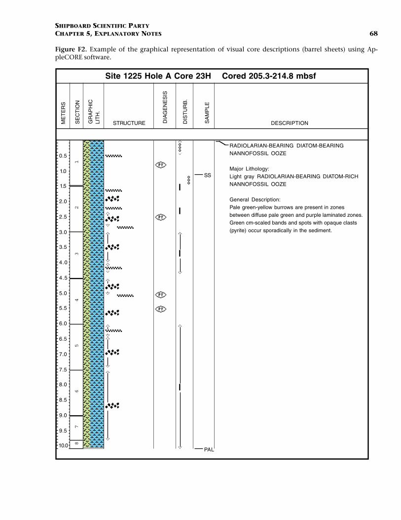
SHIPBOARD SCIENTIFIC PARTYCHAPTER 5, EXPLANATORY NOTES 68
Figure F2. Example of the graphical representation of visual core descriptions (barrel sheets) using Ap-pleCORE software.
Site 1225 Hole A Core 23H Cored 205.3-214.8 mbsf
0.5
1.0
1.5
2.0
2.5
3.0
3.5
4.0
4.5
5.0
5.5
6.0
6.5
7.0
7.5
8.0
8.5
9.0
9.5
10.0
ME
TE
RS
12
34
56
78
SE
CT
ION
GR
AP
HIC
LIT
H.
STRUCTURE DIA
GE
NE
SIS
DIS
TU
RB
.
SS
PAL
SA
MP
LE
RADIOLARIAN-BEARING DIATOM-BEARING NANNOFOSSIL OOZE
Major Lithology:Light gray RADIOLARIAN-BEARING DIATOM-RICH NANNOFOSSIL OOZE
General Description:Pale green-yellow burrows are present in zones between diffuse pale green and purple laminated zones. Green cm-scaled bands and spots with opaque clasts (pyrite) occur sporadically in the sediment.
DESCRIPTION

SHIPBOARD SCIENTIFIC PARTYCHAPTER 5, EXPLANATORY NOTES 69
Figure F3. Key to patterns and symbols used in Leg 201 barrel sheets.
Lithology
ContactsSharp ScouredUndulating Inclined
Structures
Fossils- Fish remains - Spicules
Diagenesis
Bioturbation
Drilling Disturbance
SamplesSS - Smear slide XRA - X-ray diffraction IW - Interstitial waterPPWR - Physical properties whole round PAL - Paleontology
- Bioturbation - minor - Bioturbation - moderate - Bioturbation - intense
- High-angle parallel bedding
- Low-angle parallel bedding
- Wavy parallel bedding
- Convolute bedding
- Planar lamination
- Color band
- Cross-bedding
- Normal-graded bedding
- Reverse-graded bedding
- Fining upward
- Slump
- Coarsening-upward
- Mottled
- Erosion surface - Sand lamina
- Silt lamina
- Microfault (normal)
- Thin ash layer
- Fault
- Macrofault (normal)
- Fluid escape structure
- Shell fragments
- Soupy
- Slightly disturbed
- Drilling breccia
- Very disturbed
Nannofossilooze
Foraminiferooze
Nannofossilchalk
Limestone
Dolomite
Void/No core
Whole-roundsample
Volcanic ashor tuff
Gravel
Metalliferoussediment
Sulfidesand
SulfidesiltSand
Siltysand
Clayeysand
Silt
Sandysilt
Chert
Clay
Clayeysilt
Siltyclay
Sandyclay
- Biscuit
- Moderately disturbed
- Dolomitic
- Pyrite
- Peloids
- Nodule/concretion, general
- Barite nodule/concretion
- Calcite nodule/concretion
- Calcedony/chert nodule/concretion
- Dolomite nodule concretion
- Pyrite nodule/concretion
- Cement, general
- Calcite cement
- Calcedony/chert cement
- Dolomite cement
- Carbonate nodule/concretionC
- Glauconite
- Phosphate
- Magnetite
- Calcareous
- Phosphate concretion
Gl
Fe
Ph
- Quartz cement
Ichnofossils
- Skolithos- Planolites - Zoophycos - Chondrites
Diatomooze
Diatomite
Porcellanite
Diatom-Rad.Ooze
Radiolarianooze

SHIPBOARD SCIENTIFIC PARTYCHAPTER 5, EXPLANATORY NOTES 70
Figure F4. (A) Classification scheme for siliciclastic sediment components and (B) an example for namingmixtures of biogenic and siliciclastic sediments. The terms “nannofossil” and “clay” may be replaced byany other name for siliciclastic or biogenic sediment particles (e.g., silt, sand, foraminifers, or diatoms).
100755075
Sand100
100
7575
7575
50 50
Sand
Siltysand
Clayeysand
Sandysilt
Sandyclay
Clayeyclay
Siltyclay ClaySilt
Percent biogenic material
Nannofossilooze
Nanno-fossilclay
Nannofossil-rich clay
N.-
bear
ing
clay
Cla
y
Percent siliciclastic material
A
B
Silt Clay
100 95 90 60 40 0
0 5 10 40 60 100

SHIPBOARD SCIENTIFIC PARTYCHAPTER 5, EXPLANATORY NOTES 71
Figure F5. Grain-size classification diagram for siliciclastic sediments (modified after Wentworth, 1922).
1/2
1/4
1/8
1/16
1/32
1/64
1/128
1/256
2.00
1.00
0.50
0.25
0.125
0.0625
0.0310
0.0156
0.0078
0.0039
-12.0
-8.0
-6.0
-2.0
-1.0
0.0
1.0
2.0
3.0
4.0
5.0
6.0
7.0
8.0
Gra
vel
San
dS
ilt
4096
256
64
4
Mud
Conglomerate/Breccia
Sandstone
Siltstone15.6
63
500
250
125
31
7.8
3.9
Boulder
Cobble
Pebble
Granule
Very coarse sand
Coarse sand
Medium sand
Fine sand
Very fine sand
Coarse silt
Medium silt
Fine silt
Very fine silt
0.00006 14.0 Claystone0.06 Clay
Millimeters (mm) Phi (φ) Wentworth size class Rock typeMicrometers (µm)

SHIPBOARD SCIENTIFIC PARTYCHAPTER 5, EXPLANATORY NOTES 72
Figure F6. Diagram of WRC sectioning for microbiology (MBIO). After taking syringe samples on the cat-walk, two complete, sequential, 1.5-m sections were rapidly taken to the cold room (4°–10°C). Typically,Section 3, if not visibly disturbed, was subsampled after cleaning and alcohol wiping. The first cut (boldline) was done with the ODP cutter and separated the section into a portion to be further sectioned cleanlyand anoxically in a cutting rig and one to be cut with the ODP cutter. Both sections were handled simul-taneously and in the order shown. A sample for interstitial water (IW) was the first section taken and wasimmediately given to the geochemists for processing (unless already taken on the catwalk from the adja-cent section end). The next section was for slurries, if required (nonroutine subsampling). This was rapidlycut, and at the middle cut of the liner the core was broken so that the broken surfaces were pointing down-ward after breaking (dotted line). The middles of the two broken parts were then immediately subsampled.AODC = acridine orange direct count, PFC = perfluorocarbon tracer, WRC = whole-round core, FISH = flu-orescence in situ hybridization, DNA = deoxyribonucleic acid, ATP = adenosine triphosphate, SRR = sulfatereduction rates, DIFF = diffusion experiments, AOM = anaerobic oxidation of methane, MPN = most prob-able number. CHNS = carbon, hydrogen, nitrogen, sulfur analyses.
Sections 3 and 4 cut on catwalk
AODC,CH4,PFC
RemainingWRC(x cm)
FISH(6 cm)
TurnoverH2, SO4,
MagneticsCHNS(6 cm)
FeS(5 cm)
Biomarkers(X x 5-10 cm)
DNA(X x 5 cm)
ATP(10 cm)
IW(15 cm)
Clean, anoxic cutting Clean cutting
Both sections transferred to cold room; unused portion of Section 4 returned to curation path
RemainingWRC(x cm)
TurnoverH2, SO4,
MagneticsCHNS(6 cm)
Clean, anoxic cutting Clean cutting
AOM(5 cm)
13C intobiomarkers
(10 cm)
TurnoverAc, Bi, Thy,
H3, PO4, 18O(12 cm)
DIFF(5 cm)
Cells(5 cm)
FeS(6 cm)
Biomarkers(X x 5-10 cm)
DNA(X x 5 cm)
ATP(5 cm)
Slurries, MPN,enrichments,
FISH, AODC, 13C,contamination
(14 cm)
IW(15 cm)
Clean cutting
AODC,CH4,PFC
1 6 75432
3 4
Routine subsampling of Section 3
Expanded subsampling of Sections 3 and 4
ODP catwalk cut ODP catwalk cut ODP catwalk cut
Sterile break
FISH(6 cm)
SRR(5 cm)

SHIPBOARD SCIENTIFIC PARTYCHAPTER 5, EXPLANATORY NOTES 73
Figure F7. Nitrogen-gassed cutting rig used for cutting whole-round cores (WRCs) in the cold room. Thecutting rig and the surface of the WRC are cleaned with alcohol, and the core liner is carefully cut duringrotation. Cutting blades can be sterilized. A sterile blade separates a segment from the core. The WRC seg-ment is immediately transferred to the subsampling bucket (see Fig. F8, p. 74).

SHIPBOARD SCIENTIFIC PARTYCHAPTER 5, EXPLANATORY NOTES 74
Figure F8. “Bucket” for clean and anoxic subsampling from WRC segments into sterile syringes with theLuer end removed. A 5-cm WRC segment is placed in the middle of the alcohol wiped and flamed bucketin which a steady nitrogen flow maintains anoxic conditions. The uppermost 1 cm is pushed out of thecore liner and is cleanly removed. Subcores are then taken from the central part with sterile, cut-off syringesthat are subsequently capped with sterile stoppers as shown.

SHIPBOARD SCIENTIFIC PARTYCHAPTER 5, EXPLANATORY NOTES 75
Figure F9. Scheme for inoculation of tubes for most probable number (MPN) counts of prokaryotes. Tubeswere filled with 9 mL of sterile medium and were inoculated with either sediment slurry or directly withsediment using a 5-mL syringe with the Luer end removed. The tenfold dilutions were done through threeto six steps, sufficient that the last dilutions would probably not contain growing prokaryotes. The tubesshowing positive growth after several weeks to months of incubation at a specific temperature were record-ed and used to calculate the most probable number of viable cells in the original sample (according to astatistical table). The highest dilutions showing growth were subsequently used as inoculum for new dilu-tion series, with the ultimate purpose of bringing cells into pure culture.
N2
Sterile cottonfilter for
anoxic N2
1 mL transfer after mixing
9 mL medium
Series A
Series B
Series C
Dilution: 10-1 10-2 10-3

SHIPBOARD SCIENTIFIC PARTYCHAPTER 5, EXPLANATORY NOTES 76
Figure F10. MPN counts with a microtiter plate. On a deep-well microtiter plate, four different slurry sam-ples were diluted in triplicate down to 1:106. For each sample, a row remained uninoculated as a control.The wells were sealed with a capmat, and the plate was stored in an anoxic bag with an oxygen-consumingcatalyst (Anaerocult A, Merck) and an oxygen indicator.
1 2 3 4 5 6 7 8 9 10 11 12 A
B
C
D
E
F
G
H
0.1 mL transfers
0.1 mLSlurry 1
Control
0.1 mLSlurry 3
0.1 mLSlurry 2
Control
0.1 mLSlurry 4
Dilution step
0.9 mLmedium
10-110-2 10-3
10-4 10-510-6 10-6
10-5 10-410-3 10-2
10-1

SHIPBOARD SCIENTIFIC PARTYCHAPTER 5, EXPLANATORY NOTES 77
Figure F11. Gradient culture tubes were prepared by fixing 0.5 mL of a monomer medium (Mono) on thebottom with agar. Then, substrate-free mineral medium with agar was added as a spacer, a sediment piecewas positioned, and the tube was filled with mineral medium and gassed with nitrogen on ice. MM = ma-rine salts medium.
0.5 mLsubstrates
(monomers)
0.5 mLagar
2.5 mLagar +
6 mL MM(+FeS)
2.5 cmsediment
+ 5 mL MM with
1.5% agar
0°C
N2
1 2 3 4 5

SHIPBOARD SCIENTIFIC PARTYCHAPTER 5, EXPLANATORY NOTES 78
Figure F12. Infrared thermal imaging camera on cart with reflective shield.

SHIPBOARD SCIENTIFIC PARTYCHAPTER 5, EXPLANATORY NOTES 79
Figure F13. ODP paleomagnetic coordinate system for archive and working halves with radial and verticaloverprints shown.
Working half Double line along axis of core liner
+x = North+y = East
Bottom
+z+y
+xTop
Top
Upcore
Upcore
Bottom
+x+z
+y
Archive half Single line along axis of core liner
270
000
090
180
090270
North
East
South
West
+y
+x
-z
+z
ODP magnetic direction convention
A
B

SHIPBOARD SCIENTIFIC PARTYCHAPTER 5, EXPLANATORY NOTES 80
Figure F14. Tool strings used during Leg 201. Close-up of the Formation MicroScanner (FMS) four arms andthe 16 individual buttons.
Cablehead
Telemetry cartridge
DSIDipole SonicShear Imager
FMSFormation
MicroScanner
tool zero
GPITGeneral PurposeInclinometry Tool
FormationMicroScanner
cartridge
30 m
NGTNatural Gamma
Ray Spectrometry Tool
Centralizer
Centralizer
FMS-Sonic
Caliper
tool zero
Cablehead
Telemetry cartridge
HNGSHostile EnvironmentGamma Ray Sonde
APSAccelerator
Porosity Sonde
HLDSHostile EnvironmentLitho-Density Sonde
TAPTemperature/Acceleration/
Pressure tool
32 m
DIT-EDual Induction
Tool
Triple Combo

SHIPBOARD SCIENTIFIC PARTYCHAPTER 5, EXPLANATORY NOTES 81
Table T1. Definitions of terms used in microbiology sampling.
Term Definition
Aseptic A clinical definition referring to freedom from pathogens. Clinical conditions are not applicable to ODP operations.
Sterile The most stringent category used during Leg 201. Sterile indicates the absence of contaminating prokaryotic cells that are capable of metabolism and growth and their nucleic acids.
Clean Defined as giving careful consideration and effort to avoid cross-contamination. May involve ethanol washing, flaming instruments, etc., and may approach sterile conditions.
Anaerobic A property of organisms indicating the ability to live without oxygen. Also a property of a method (“anaerobic cultivation”) or of laboratory cultivation equipment (“anaerobic chambers”).
Anoxic Property of an oxygen-free environment such as used in a glove bag or N2-flushed sampling bucket.

SHIPBOARD SCIENTIFIC PARTYCHAPTER 5, EXPLANATORY NOTES 82
Table T2. Definitions of sampling codes and packing types.
Notes: FISH = fluorescent in situ hybridization. SIMS = secondary ion mass spectrometry. WRC = whole-round core. — = addi-tional sample specification may be appended to sample code.
Codes Definition
Sampling codes:FISH— FISH and FISH-SIMSH3S Tritiated hydrogen turnover experimentsABTP Thymidine incorporation, bicarbonate, and acetate turnover rate measurementsO18B 18O stable isotope turnover experimentsPO4B Determination of 18O in phosphateSRRF Sulfate reduction rate measurementsH2S Hydrogen turnover rate measurementsCNSS Samples for carbon, nitrogen, and sulfur determination (geochemistry laboratory)CHNSF Samples for prokaryotic magnetic particlesBIOM— Biomarker samplesDIFFF Core for diffusion experimentsCELLS Sediment used for isolating individual cellsAODC Acridine orange direct counts for prokaryotic cell enumerationFESF WRC for determination of Fe, Mn, and S solid-phase concentrations, mineralogy, and isotope distributionsSRRWRF WRC for sulfate reduction, pressure, and temperature experimentsAMO— Samples for measurements of rates of anaerobic oxidation of methaneHTEW Enrichments for thermophilesSLUR Sediment for master slurrySLURJ Enrichments for psychrophilic methanogensSLURA Enrichments for psychrophilesSLURB Enrichments for sulfate-reducing psychrophilesFISHWR2 Samples for FISH-SIMSFISHWR Samples for FISH-SIMSDNA— Samples for microbial molecular analysisDNAODP Archived deep-frozen WRC samples for microbial molecular analysisATPS Adenosine triphosphate samplesAIELLO Residual material from microbiology, used for lithostratigraphic interval and descriptionPRIEUR WRC for enrichments
Packing types:Polybag Sterile polyethylene sample bagAl-bag Aluminum gas-tight bagAnaer. jar N2-flushed sample jarVacuum pack Air removed from Al bag before heat sealingAnaerocult A Small trays of metallic Fe, bicarbonate, and citrate (Merck) that scrub O2 from a gas-tight bag and produce CO2 when wetted

SHIPBOARD SCIENTIFIC PARTYCHAPTER 5, EXPLANATORY NOTES 83
Table T3. Marine medium salts solution used as thebasis for psychrophilic and mesophilic media.
Notes: Adjust pH to 7.2–7.4 with sterile 1-M HCl or sterile 1-MNa2CO3. * = Widdel et al. (1983), † = Widdel (1980). ‡ = mixtureof 10 vitamins, concentrated fivefold (after Balch et al., 1979).
Component Concentration
Distilled water 1000 mL/LNaCl 24.32 g/LMgCl2·6H2O 10 g/LCaCl2·2H2O 1.5 g/LKCl 0.66 g/LNa2SO4 4.0 g/LTrace element solution (SL 10)* 1 mL/LKBr (0.84 M) 1 mL/LH2BO2 (0.4 M) 1 mL/LSrCl2 (0.15 M) 1 mL/LNH2Cl (0.4 M) 1 mL/LKH2PO4 (0.04 M) 1 mL/LNaF (0.07 M) 1 mL/LNa2SeO3 (10–7 M)† 1 mL/LNa2WoO4 (10–7 M)† 1 mL/L
Autoclave, cool under N2, then add the following from sterile stock solutions:NaHCO3 (1 M) 30 mL/LVitamin solution‡ 2 mL/LFeCl2 (1 M) in 0.1-M HCl 0.5 mL/LNa2S (1 M) 1.2 mL/L

SHIPBOARD SCIENTIFIC PARTYCHAPTER 5, EXPLANATORY NOTES 84
Table T4. Media used for cultivation of psychrophiles and mesophiles.
Notes: MM = marine medium salts solution (see Table T3, p. 83). EDTA = disodium ethylenediaminetetraacetate. * = for AmOx and NiOxthe chemicals were dissolved in 1 L filtered seawater and the pH was adjusted with HCl or NaOH. The solution was sterilized by auto-claving for 20 min at 121°C. After cooling, 1 mL of sterile-filtered iron(III) solution was added. Sterile tubes with 9 mL medium eachwere inoculated with 1 mL of a nitrite-oxidizing medium (NiOx).
Medium Components Concentration Comments
Mono: monomer Amino acids: alanine, arginine, asparagine, asparagic acid, cystine, glutamine, glutamic acid, glycine, histidine, isoleucine, leucine, lysine, methionine, phenylalanine, proline, serine, threonine, tryptophane, tyrosine, and valine
0.01 M Prepare in MM
Short chain fatty acids (sodium salts): formate, acetate, propionate, butyrate, valerate, and capronate
0.01 M
Other organic acids: malate, fumarate, succinate, and lactate 0.01 Mn-alcohols: methanol, ethanol, propanol, and butanol 0.01 MGlycerol 0.01 MGlucose 0.01 M
Poly: polymer Chitin, xylane, cellulose, and peptone 0.05% Prepare in MM
Aro: aromatic compounds and long-chain fatty acids
Aromatic compounds (sodium salts): salicylate, 3-OH-benzoate,3-OH-benzaldehyde, vanillate, vanillin, p-coumarate, ferulate, sinapinate, syringate, and syringaldehyde
0.05 M Prepare in MM
Fatty acids (sodium salts): C14–C20 0.05 M
Lac: lactate Sodium lactate 5.0 M Prepare in MM
No SO4: sulfate-free Ti(III) citrate 0.5 M Prepare in MM (omit Na2SO4, Na2S, and FeCl2)
Sed: sediment extract N-[2-hydroxyethyl]piperazine-N´-[2-ethane-sulfonic acid] buffer 2.38 g/L Prepare in MM (omit NaHCO3, vitamins, Na2S, and FeCl2) and adjust pH to 7.2–7.4. Use this solution to extract sediment at 80°C (see “Enrichments near In Situ Temperatures,” p. 29).
To sediment extract, after heating add the following:Vitamins, Na2S, and FeCl2NaHCO3 0.2 g/L
A-bas: autotrophic basalt NaCl 24 g/L Dissolve salts in deionized water, and autoclave 20 min at 121°CMgCl2·6H2O 10 g/L
KCl 0.5 g/LNa2SO4 4 g/LNH4Cl 0.25 g/LCaCl2 1.5 g/LKH2PO4 0.2 g/L
AmOx: ammonium oxidizing medium
NH4Cl 0.64 g/L Dissolve 10 mg FeCl3·6H2O in 0.3 mL 1-N HCl, add 10 mL deionized water, and then add and dissolve 60 mg EDTA.*
KH2PO4 0.1 g/LMgCl2·6H2O 0.2 g/LCaCO3 2.0 g/LFeCl3·6H2O solution 1 mL/L
NiOx: nitrite-oxidizing medium
NaNO2 0.76 g/L NaNO2 is used instead of NH4Cl; the preparation is the same as for AmOx.*NH4Cl 0.64 g/L
KH2PO4 0.1 g/LMgCl2·6H2O 0.2 g/LCaCO3 2.0 g/LFeCl3·6H2O solution 1 mL/L
Methylo: methylotrophs Agar 15 g/L Dissolve chemicals in 1 L filtered seawater and autoclave for 20 min at 121°C. After cooling to ~60°C, add 5 mL of sterile-filtered methanol. Pour on agar plates; store plate, wrapped in parafilm, at 4°C to minimize evaporation. Plates are inoculated with 0.1-mL aliquots from sample dilution series made using sterile-filtered seawater.
NH4Cl 0.4 g/LKH2PO4 0.6 g/LNa2HPO4·7H2O 1.8 g/LCaCl2 30 mg/LFeCl3·6H2O 1 mg/L

SHIPBOARD SCIENTIFIC PARTYCHAPTER 5, EXPLANATORY NOTES 85
Table T5. Media used for cultivations at 25°, 50°, and 80°C. (See table notes. Continued on nextpage.)
Medium ComponentsConcentration
(% wt/vol) Comments
201-1: Heterotrophic sulfur reducer medium Yeast extract 0.1 Prepare in MJ under N2 headspacePeptone 0.1Glucose 0.05Na2S 0.05Elemental sulfur 3Wolfe’s vitamin solution*
201-2: Heterotrophic Fe(III) reducer medium Yeast extract 0.1 Prepare in MJ under N2 headspacePeptone 0.1Glucose 0.05Na2S 0.05Ferrihydrite 1Magnetite 1Wolfe’s vitamin solution*
201-3: Heterotrophic nitrate reducer medium Yeast extract 0.1 Prepare in MJ under N2 headspacePeptone 0.1Glucose 0.05Na2SO4 0.05NaNO3 1Wolfe’s vitamin solution*
201-4: Heterotrophic sulfate reducer medium Sodium lactate 0.05 Prepare in MJ under N2 headspaceSodium acetate 0.05Sodium formate 0.05Sodium fumarate 0.05Glucose 0.05Na2SO4 0.1Na2S 0.05Cystein-HCl 0.05Wolfe's vitamin solution*
201-5: Autotrophic H2-oxidizing sulfate reducer medium
NaHCO3 0.15 Prepare in MJ under 80% H2 + 20% CO2 headspaceNa2SO4 0.1Na2S 0.05Cystein-HCl 0.05Wolfe’s vitamin solution* 0.15
201-6: Autotrophic HS–/S2O32–/S0 oxidizing
Fe(III) or nitrate reducer mediumNaHCO3 0.15 Prepare in MJ under 70% N2 + 30% CO2 headspaceNa2S2O3 0.1Elemental sulfur 3Ferrihydrite 0.05NaNO3 0.05Na2S 0.025Wolfe’s vitamin solution*
201-7: Micro-aerobic, autotrophic HS–/S2O32–/
S0 oxidizing Fe(III)/NO3– reducer medium
NaHCO3 15 Prepare in MJ under 68.5% N2 + 28.5% CO2 + 3% O2 headspaceNa2S2O3 0.1
Elemental sulfur 3Ferrihydrite 0.05NaNO3 0.05Na2S 0.025Wolfe’s vitamin solution*
201-8: Methanogen medium NaHCO3 0.15 Prepare in MJ under 80% H2 + 20% CO2 headspaceSodium acetate 0.05Sodium formate 0.05Methanol 0.05Na2S 0.05Cystein-HCl 0.05Magnetite 0.05Wolfe’s vitamin solution*
201-9: Autotrophic NH4 + oxidizing Fe(III)/
NO3– reducer medium
NaHCO3 0.15 Prepare in MJ under 70% N2 + 30% CO2 headspaceNH4Cl 0.1Ferrihydrite 0.1NaNO3 0.1CuSO4 0.05Wolfe’s vitamin solution*
201-10: Micro-aerobic, autotrophic NH4+
oxidizing Fe(III)/NO3– reducer medium
NaHCO3 0.15 Prepare in MJ under 68.5% N2 + 28.5% CO2 + 3% O2 headspaceNH4Cl 0.1
Ferrihydrite 0.1

SHIPBOARD SCIENTIFIC PARTYCHAPTER 5, EXPLANATORY NOTES 86
Notes: MJ = artificial seawater solution (see Table T6, p. 87). * = added at 1 mL/L; Freier et al., 1988.
NaNO3 0.1CuSO4 0.05Wolfe’s vitamin solution*
201-11: Extremely halophilic archaea (genus Haloarcula) medium
NaCl 20.8 Prepare in MJ under air headspace; pH (25°C) = 7.2Yeast extract 1.0MgSO4·7H2O 4.7CaCl2 0.05MnCl2 0.013Wolfe’s vitamin solution*
Medium ComponentsConcentration
(% wt/vol) Comments
Table T5 (continued).

SHIPBOARD SCIENTIFIC PARTYCHAPTER 5, EXPLANATORY NOTES 87
Table T6. MJ solution* used as the basis for 25°, 50°,and 80°C cultivation media.
Notes: MJ = artificial seawater solution. * = Leg 201 version. AdjustpH to 7.2 at 25°C with NaOH. † = Balch et al. (1979).
Component Concentration
NaCl 30.g/LNa2HPO4 0.14 g/LCaCl2·2H2O 0.14 g/LMgCl2·6H2O 7.58 g/LNH4Cl 0.25 g/LKCl 0.33 g/LNa2SeO3·5H2O 0.5 mg/LFe(NH4)2(SO4)2·6H2O 0.01 g/LWolfe’s trace mineral solution† 10.mL/L

SH
IPB
OA
RD
SC
IEN
TIFIC P
AR
TY
CH
AP
TE
R 5
, EX
PL
AN
AT
OR
Y N
OT
ES
88
Table
Notes: M nd buffer equilibrated at room temperature. No cor-recti de and buffer equilibrated for 30 min at 60°C. Buffervalue
Ferm: h adspace
H2/HCO H2 headspace
H2/HCO H2 headspace
H2/HCO H2 headspace only)cted sites)
C-18 lip adspace
SRB: he adspace
Chlor: c H2 headspace
methylmeth
N2 headspace
25°C
CH4-ac N2 headspace
25°C
T7. Media used for cultivations at 60°C.
SSM = marine sea-salt media (see Table T8, p. 89). * = Freier et al., 1988. pH25°C = pH meter was calibrated with the electrode aon for the sea salt concentration was made. pH60°C = pH meter, with temperature probe connected, was calibrated with the electros were temperature corrected. No correction was made for the sea salt.
Medium Components Concentration Comments
eterotrophic fermenter Na2S 2 mM Prepare in MSSM under N2 heCystein HCl 2 mM MPNs pH60°C = 7.95
A) glucose, fructose, and mannose 0.2%, wt/vol each Enrichments pH60°C = 8.8B) xylose and ribose 0.2%, wt/vol eachC) xylose and ribose + 25 mM NaS2O3
2– 0.2%, wt/vol each
3–: acetogenic/methanogenic Na2CO3 15 mM (total 25–30 mM with
near-equal amount from sea salt)Prepare in MSSM under 100%MPNs pH60°C = 7.95 (8.0)Enrichments pH60°C = 8.8
3–/FeIII: iron(III) reducer Na2CO3 15 mM (total 25–30 mM with
near-equal amount from sea salt)Prepare in MSSM under 100%MPNs pH60°C = 7.8
Fe(III) 90 mM Enrichments pH60°C = 8.3
3–/MnIV: manganese(IV) reducer Na2CO3 15 mM (total 25–30 mM with
near-equal amount from sea salt)Prepare in MSSM under 100%MPNs pH60°C = 7.8 (Site 1231
Mn(IV)(HO,O)x 15 mM Enrichments pH60°C = 7.8 (sele
o: lipolytic microorganism Cystein HCl 0.15 g Prepare in MSSM under N2 heYeast extract (total of 0.2%) 0.15% MPNs pH60°C = 7.8Na2SO4 10 mM Enrichments pH60°C = 9Olive oil 20 ml
terotrophic sulfate reducer Na2SO4 20 mM Prepare in MSSM under N2 heCystein HCl 2 mM Enumerations pH60°C = 8.0A) Lactate 25 mM Enrichments pH60°C = 8.6
Acetate 25 mMPropionate 5 MButyrate 5 mM
B) Benzoate (only pH = 8) 10 mM Enumerations pH60°C = 8.0
hlorate reducer Na2CO3 (total bicarbonate/carbonate to be determined later)
15 mM (total 25 mM + equal unknown amount from the salt)
Prepare in MSSM under 100%
Na chlorate 5 mM
amine: methylamine-utilizing anogens
Na2S 2 mM Prepare in MSSM under 100%Cystein HCl 2 mM MPNs pH25°C = 8.4Methylamine 2.5 mM Enrichments pH25°C = 8.4Trimethylamine 2.5 mM Site 1229 only; use at 60° and
e: acetate-utilizing methanogens Na2S 2 mM Prepare in MSSM under 100%Cystein HCl 2 mM MPNs pH25°C = 8.3Acetate 5 mM Enrichments pH25°C = 8.3
Site 1229 only; use at 60° and

SHIPBOARD SCIENTIFIC PARTYCHAPTER 5, EXPLANATORY NOTES 89
Table T8. MSSM used as the basis for 60°C cultiva-tions.
Notes: MSSM = marine sea-salts media. Prepare solution in deion-ized, distilled water. * = Freier et al., 1988. pH (25°C) wasadjusted to 8.5 and 10.0, respectively, before autoclaving. ThepH after autoclaving and at 60°C is ~0.5 to 1.2 pH units(depending on media supplements) more acidic.
Component Concentration
Sigma sea salt 40.g/LNa2HPO4·H2O 2.mM/LModified (Ni, W) Wolfe’s mineral 0.25 mL/LWolfe’s vitamin solution* 5.mL/LYeast extract 0.5%/LNH4Cl 0.1%/LNa2CO3 25.mM/L
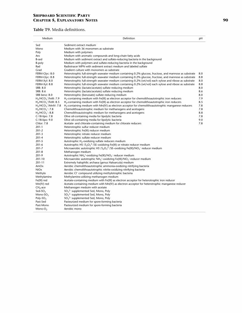
SHIPBOARD SCIENTIFIC PARTYCHAPTER 5, EXPLANATORY NOTES 90
Table T9. Media definitions.
Medium Definition pH
Sed Sediment extract mediumMono Medium with 36 monomers as substratePoly Medium with polymersAro Medium with aromatic compounds and long-chain fatty acidsB-sed Medium with sediment extract and sulfate-reducing bacteria in the backgroundB-poly Medium with polymers and sulfate-reducing bacteria in the backgroundRad Radiotracer MPN with sediment extract medium and labeled sulfateGrad Gradient culture with monomers as substrateFERM-Glyc: 8.0 Heterotrophic full-strength seawater medium containing 0.2% glucose, fructose, and mannose as substrate 8.0FERM-Glyc: 8.8 Heterotrophic full-strength seawater medium containing 0.2% glucose, fructose, and mannose as substrate 8.8FERM-Xyl: 8.0 Heterotrophic full-strength seawater medium containing 0.2% (wt/vol) each xylose and ribose as substrate 8.0FERM-Xyl: 8.8 Heterotrophic full-strength seawater medium containing 0.2% (wt/vol) each xylose and ribose as substrate 8.8SRB: 8.0 Heterotrophic (lactate/acetate) sulfate reducing medium 8.0SRB: 8.6 Heterotrophic (lactate/acetate) sulfate reducing medium 8.6SRB benz: 8.0 Heterotrophic (benzoate) sulfate reducing medium 8.0H2/HCO3
–/FeIII: 7.9 H2-containing medium with Fe(III) as electron acceptor for chemolithoautotrophic iron reducers 7.9H2/HCO3
–/FeIII: 8.5 H2-containing medium with Fe(III) as electron acceptor for chemolithoautotrophic iron reducers 8.5H2/HCO3
–/MnIV: 7.8 H2-containing medium with Mn(IV) as electron acceptor for chemolithoautotrophic manganese reducers 7.8H2/HCO3
–: 7.8 Chemolithoautotrophic medium for methanogens and acetogens 7.8H2/HCO3
–: 8.8 Chemolithoautotrophic medium for methanogens and acetogens 8.8C-18-lipo: 7.8 Olive oil-containing media for lipolytic bacteria 7.8C-18-lipo: 9.0 Olive oil-containing media for lipolytic bacteria 9.0Chlor: 7.8 Acetate- and chlorate-containing medium for chlorate reducers 7.8201-1 Heterotrophic sulfur reducer medium201-2 Heterotrophic Fe(III) reducer medium201-3 Heterotrophic nitrate reducer medium201-4 Heterotrophic sulfate reducer medium201-5 Autotrophic H2-oxidizing sulfate reducers medium201-6 Autotrophic HS–/S2O3
2–/SE–oxidizing Fe(III) or nitrate reducer medium201-7 Microaerobic autotrophic HS–/S2O3
2–/SE–oxidizing Fe(III)/NO3– reducer medium
201-8 Methanogen medium201-9 Autotrophic NH4
+-oxidizing Fe(III)/NO3– reducer medium
201-10 Microaerobic autotrophic NH4+-oxidizing Fe(III)/NO3
–-reducer medium201-11 Extremely halophilic archaea (genus Haloarcula) mediumAmOx Aerobic chemolithoautotrophic ammonia-oxidizing nitrifying bacteriaNiOx Aerobic chemolithoautotrophic nitrite-oxidizing nitrifying bacteriaMethylo Aerobic Cl– compound utilizing methylotrophic bacteriaMethylamine Methylamine-utilizing methanogen mediumFe(III) red Acetate-containing medium with Fe(III) as electron acceptor for heterotrophic iron reducerMn(IV) red Acetate-containing medium with Mn(IV) as electron acceptor for heterotrophic manganese reducerCH4-ace Methanogen meduim with acetateSed-SO3 SO3
2– supplemented Sed, Mono, PolyMono-SO3 SO3
2– supplemented Sed, Mono, PolyPoly-SO3 SO3
2– supplemented Sed, Mono, PolyPast-Sed Pasteurized medium for spore-forming bacteriaPast-Mono Pasteurized medium for spore-forming bacteriaMono-O2 Aerobic mono

SHIPBOARD SCIENTIFIC PARTYCHAPTER 5, EXPLANATORY NOTES 91
Table T10. Enrichment inoculations, Holes 1225A and 1226B.
Note: WRC = whole-round core, FISH = fluorescent in situ hybridization.
Enrichment Comments
Sample 201-1225A-35H-CC, incubated at 10°C:Tube 1: with Fe(OH)3 and MnO2 ControlTube 2: no Fe(OH)3 and MnO2 ControlTube 3: with Fe(OH)3 and MnO2 Basalt piece taken directly from the sample, not washed, not crushedTube 4: with Fe(OH)3 and MnO2 First basalt piece washed with salt solution, crushed in chipsTube 5: no Fe(OH)3 and MnO2 First basalt piece washed with salt solution, crushed in chipsTube 6: with Fe(OH)3 and MnO2 Second basalt piece washed with salt solution, crushed in chipsTube 7: no Fe(OH)3 and MnO2 Second basalt piece washed with salt solution, crushed in chipsTube 8: with Fe(OH)3 and MnO2 First basalt piece washed with salt solution, additional washing with 3-M HCl for 1 min, crushed in chipsTube 9: no Fe(OH)3 and MnO2 First basalt piece washed with salt solution, additional washing with 3-M HCl for 1 min, crushed in chipsTube 10: with Fe(OH)3 and MnO2 First basalt piece washed with salt solution, crushed in very small chipsTube 11: no Fe(OH)3 and MnO2 First basalt piece washed with salt solution, crushed in very small chips
Core 201-1226B-47X, incubated at 23°C:Tube 1: with Fe(OH)3 and MnO2 ControlTube 2: no Fe(OH)3 and MnO2 ControlTube 3: with Fe(OH)3 and MnO2 Sediment, FISH WRCTube 4: no Fe(OH)3 and MnO2 Sediment, FISH WRCTube 5: with Fe(OH)3 and MnO2 Basalt piece washedTube 6: no Fe(OH)3 and MnO2 Basalt piece washedTube 7: with Fe(OH)3 and MnO2 Basalt piece washed with salt solution, additional washing with 3-M HCl for 1 minTube 8: no Fe(OH)3 and MnO2 Basalt piece washed with salt solution, additional washing with 3-M HCl for 1 minTube 9: with Fe(OH)3 and MnO2 ControlTube 10: no Fe(OH)3 and MnO2 ControlTube 11: with Fe(OH)3 and MnO2 Washing solutionTube 12: no Fe(OH)3 and MnO2 Washing solution

SHIPBOARD SCIENTIFIC PARTYCHAPTER 5, EXPLANATORY NOTES 92
Table T11. Sample preparation and fixation for FISH analysis.
Note: FISH = fluorescence in situ hybridization.
Solution Components Concentration Comments
Phosphate buffered saline (PBS):
NaCl 8 g/L Prepare in 1L of sterile-filtered water; adjust pH to 7.2–7.5
KCl 0.2 g/LKH2PO4 0.2 g/LNa2HPO4·2H2O 1.44 g/L
4% Formaldehyde/PBS buffer:
A) PBS buffer: 25 mL/L Prepare at least once per week; adjust pH to 7.2–7.5
37% formaldehyde solution
2.7 mL
B) PBS buffer: 25 mL Heat to 60°CParaformaldehyde 1 g/L White powder (toxic)NaOH A few microliters To dissolve paraformaldehyde
Fixation procedure Comments
Add 1.5 mL 4% formaldehyde/PBS buffer to 0.5-cm sample or cell suspension in a 2-mL screwtop microfuge tube.
Samples are taken in 5-mL syringes from cold room on a regular basis and are fixed immediately.
Keep cold on ice for 1–24 hr. This can also be done at 4°C or room temperature.
Centrifuge at 13,000 rpm in the table-top centrifuge.
Optimally at 4°C.
Remove supernatant, add 1.5 mL PBS buffer, and suspend cells/sediment on whirl mixer.
Repeat these two washing steps to remove formaldehyde.
Centrifuge at 13,000 rpm in the table-top centrifuge.
Optimally at 4°C.
Remove supernatant and add 1.5 mL of 1:1 mix of PBS buffer/100% ethanol.
Resuspend sample on whirl mixer. Use samples directly for FISH or keep at –20°C for a maximum of several months. The mixture should remain liquid and therefore must not be frozen at –80°C. Storage at 4°C is also possible for some time.

SHIPBOARD SCIENTIFIC PARTYCHAPTER 5, EXPLANATORY NOTES 93
Table T12. Hybridization procedure for FISH analysis.
Notes: FISH = fluorescence in situ hybridization. PBS = phosphate buffered saline, DAPI = 4′,6-diamindino-2-phenylindole, Tris =tris(hydroxymethyl)amino methane, SDS = sodium dodecyl sulfate, EDTA = disodium ethylenediaminetetraacetate, UV = ultraviolet. * =concentrations of NaCl in washing buffer (48°C) are given at different concentrations of formamide in hybridization buffer (46°C). Thefirst number of each pair is the formamide concentration in the buffer (vol%) and the second number is the NaCl concentration in thewashing buffer (mM): 1, 900; 5, 636; 10, 450; 15, 318; 20, 225; 25, 159; 30, 112; 35, 80; 40, 56; 45, 40; 50, 28; 55, 20; 60, 14; 65, 10;70, 7; 75, 5; 80, 3.5.
Solution Components Volume Final concentration
Hybridization buffer: 5-M NaCl 360 µL 900 mM1-M Tris/HCl (pH = 7.5) 40 µL 20 mMFormamide Vol% depending on probeDistilled H2O Add to 2 mL10% SDS 2 µL 0.1%
Washing buffer: 5-M NaCl Depending on %* 900 mMFormamide in hybridization buffer (see above) *1-M Tris/HCl (pH = 7.5) 1 mL 20 mM0.5-M EDTA 500 µL 5 mMDistilled H2O Add to 50 mL10% SDS 50 µL 0.01%
Hybridization procedure Comments
Resuspend sample and transfer 20–100 µL of aliquot to 500 µL of a 1:1 mix of PBS/ethanol in a 2-mL microfuge tube.
Optional dilution step.
Sonicate aliquot for 20–30 s at low intensity using 1-s sonication pulses. If required, the sonicated sample can be further diluted.
For fine-particle sediments, vortexing is fine.
Place GTTP filter (pore size = 0.2 µm) on glass filter surface (shiny side on top). Add 10–100 µL of fixed suspension to 5–10 mL of PBS buffer into the filter tower and filter this volume onto the membrane filter.
Air-dry filters can be stored in Petri dishes at –20°C until hybridization. The procedure can be paused here if shipboard schedule demands it.
Prepare 2 mL of hybridization buffer in a microfuge tube (see above).
For the hybridization mixtures, add 2 µL of probe working solution (50–200 ng probe/µL) to 18 µL of hybridization buffer in a 0.5-mL microfuge tube.
Keep probe solutions dark and on ice.
Cut filter in quarters with razor blade and place the pieces on a glass slide, upside facing up. Do not touch filter surface with fingers. Several filters can be placed on one slide and simultaneously hybridized with the same probe. Quarters may be marked with incisions if different probes will be applied.
Put a piece of blotting paper into a 50-mL polyethylene tube and soak it with the remaining hybridization buffer.
JOIDES Resolution toilet paper can serve as blotting paper.
Add hybridization mix on the samples, one 20-µL drop per filter section, and place the slide with filter sections into the polyethylene tube in a horizontal position.
Make sure the hybridization mix does not run off.
Incubate 1.5–2 hr at 46°C. Do not exceed 3 hr.
Prepare 50 mL of washing buffer (see above) in a polyethylene tube and pre-warm at 48°C in a water bath.
Quickly transfer filter sections into preheated washing buffer and incubate for 15 min at 48°C.
Pour washing buffer with filter sections into a Petri dish. Pick filter sections and rinse them by placing them into a Petri dish with distilled H2O for several seconds, then let them air-dry on blotting paper.
For counterstaining, put filter sections on glass slides (side with bacterial cells facing up), cover with 50 µL DAPI solution (1 mg/L), and incubate for 3 min. Afterward, rinse filter sections briefly in distilled H2O, wash them for several seconds in 80% ethanol to remove unspecific DAPI staining, and air-dry.
Filters on glass slide are embedded in a 4:1 mix of Citifluor and Vecta Shield and are covered with a cover slide. The filter sections have to be completely dried before embedding; otherwise, a fraction of cells will detach during inspection.
It is also possible to use Citifluor or Vecta Shield without a coverslip.
Double-stained and air-dried preparations as well as filters mounted on slides can be stored in the dark at –20°C for several months without substantial loss of probe fluorescence.
Probe-conferred fluorescence fades much more rapidly than DAPI fluorescence in the microscopic image. For counting, it is therefore safer to first quantify specifically stained cells in green excitation and subsequently all cells from the same field in UV excitation (DAPI).

SHIPBOARD SCIENTIFIC PARTYCHAPTER 5, EXPLANATORY NOTES 94
Table T13. Sample preparation and 13C experiments for FISH-SIMS.
Notes: DGH media were prepared prior to the cruise. * = 0.25 g NaS was added to reduce the media. Themedia was dispensed in an anoxic environment with 10 mL added to each 125-mL serum vial. † = mediawas degassed with N2/CO2, neutralizing the NaOH and resulting in a final pH of 6.8.
Sample preparation:A 5-cm3 subcore was injected into a sterile 50-mL centrifuge tube containing 10 mL 1:1 ethanol/PBS solution; the
suspension was stored at –20°C.At select sites:
1) A 5-cm3 subcore was fixed in 3.7% formaldehyde in PBS for 1–24 hr.2) The sample was washed twice with PBS (using standard FISH protocols; see Table T11, p. 92, FISH fixation).3) After washing, the sample was stored at –20°C in a sterile 50-mL centrifuge tube containing 10 mL 1:1 ethanol/PBS.
The residual round core from which the subcores had been removed was frozen at –80°C for storage.
Experiments on incorporation of 13C-labeled substrates:1) Sterile bottles with 10 mL of reduced DGH media (see below) and a labeled substrate were sealed in an 80% N2/20%
CO2 atmosphere during precruise preparation. In some cases, the headspace also included 20 mL of nonlabeled methane.
2) For each sample, 10 mL of 25% sediment slurry was injected into an experiment bottle and incubated at 4°C.3) To terminate incubation, 40 mL of headspace gas was removed (at the rear of the ship to avoid 13C contamination of
geological samples), and 20 mL of filtered ethanol was injected into the bottle. Samples were then stored at –20°C. Postcruise, samples will be fixed in 3.7% formaldehyde, washed with filtered PBS buffer, and ultimately stored in a 1:1 ethanol/PBS solution at –20°C.
Each bottle had one of three possible 13C labeled substrates: glucose, acetate, or methane. Glucose and acetate concentrations were 1 mg/mL of media with half of the substrate 13C labeled, whereas methane concentrations were 20 mL/per serum bottle with one-fourth of the methane 13C labeled.
DGH media preparation*:Component: NaCl Concentration: 10 g/500 mL
Na2SO4 1.5 g/500 mLKH2PO4 0.1 g/500 mLNH4Cl 0.15 g/500 mLKCl 0.15 g/500 mLCaCl2·H2O 0.1 g/500 mLMgCl2·6H2O 0.15 g/500 mLWolfe trace elements0.2% (NH4)2Fe(SO4)2 0.5 mL/500 mL10% NaOH† 1.5 mL/500 mLddH20 500 mL/500 mL

SHIPBOARD SCIENTIFIC PARTYCHAPTER 5, EXPLANATORY NOTES 95
Table T14. Procedure for sulfate reduction measurements.
1) In the cold room, whole-round cores were cleanly and anoxically cut and transferred into an N2-gassed (filtered) sampling bucket. After removing 1 cm of surface sediment, four 5-cm3 subsamples were taken with sterile syringes with the Luer end removed.
2) The syringes were closed gas-tight with sterile butyl rubber and placed in a N2-filled aluminum bag for transport.
3) After transfer to the radioisotope van, the syringe samples were kept at in situ temperature in a thermostated incubator to equilibrate before further processing.
4) To start the experiment, 10 µL of a 35SO42– solution was injected by microsyringe into three of the four parallel
syringes through the butyl rubber stopper and along a 1- to 2-cm line in the middle of the sediment. The radiotracer stock solution for injections was made up as 35SO4
2– in sterile saline solution (containing sulfate concentrations appropriate for the site and depth) by diluting a commercial stock solution (Perkin-Elmer/NEN, 185 MBq).
5) Three types of blank measurements were performed:a. From each vial of radiolabeled solution, a 10-µL aliquot was fixed in Zn acetate solution. b. At selected depths, a “time-zero” control was performed on a syringe subsample. The radiolabeled sulfate was
injected into the sediment and allowed to incubate for ~30 min (<1% of the total incubation time), after which time it was fixed in Zn acetate solution.
c. A third “killed” control consisted of adding the sediment to the Zn acetate solution. After 30 min, 10 µL of 35SO4
2– was then added to the Zn acetate-sediment slurry.All controls are distilled and counted as for live samples.
6) The radiolabeled syringe samples were placed in N2-filled gas bags. Two squares of an oxygen scrubber tray (Anaerocult A; Merck) were added to the bag and wetted. The bags were sealed and placed in the appropriate incubator.
7) At the conclusion of the incubation period, ranging from 7 to 42 days, the bacterial activity was stopped by mixing the sediment into pre-tared 50-mL Corning screw-top vials containing 14 mL of 20% (w/v) zinc acetate solution. The zinc solution kills the bacteria and preserves any free sulfides by precipitating them as ZnS.
8) These fixed samples were transported frozen to the shore-based institute in Bremen, Germany, for further processing. For safe handling and transport, all vials were packed break-proof in original styrofoam, double-bagged, and packed in a International Air Transport Association approved carton (shipped as UN2910-Radioactive material, excepted package—limited quantity of material).
9) The processing (as modified from Fossing and Jørgensen, 1989) involves the separation of the injected 35SO42–
and the reduced 35S-sulfide (in total reduced inorganic sulfides) in chromous acid solution by cold distillation of the released H2
35S into Zn-acetate traps. By measurement of the 35SO42– and Zn35S radioactivities on a liquid
scintillation counter, the fraction of sulfate reduced during the experiment can be determined. This is converted to total amount of sulfate reduced per unit time (nmol SO4
2–/cm3/day) based on the interstitial water concentration of sulfate, the porosity, and the incubation time (cf. Jørgensen, 1978).

SHIPBOARD SCIENTIFIC PARTYCHAPTER 5, EXPLANATORY NOTES 96
Table T15. Procedure for methanogenesis and acetate turnover (14C tracer) experiments.
1) Syringe subsamples (5 mL) sealed with a butyl suba-seal were stored in an N2-flushed anaerobic jar during storage in the constant temperature room.
2) These subsamples were transferred to the isotope van and kept at in situ temperature in an appropriate incubator to equilibrate.
3) The control sample for each sediment depth was prechilled (4°C) prior to injection with the isotope.
4) An injection microsyringe was flushed thoroughly with the isotope (at least five times), ensuring that there were no air bubbles. The subsample was placed in the injection rig, followed by the injection microsyringe, by inserting the needle through the suba-seal. An exact amount of isotope was delivered evenly along the length of the sediment in the sample by pulling back the barrel of the microsyringe completely to the stop. When removing the microsyringe from the rig, the volume injected was checked.
5) Volumes of radiotracer injected into each syringe subsample and for each individual tracer was 7.2 µL (4.8 µCi) of sodium 14C-bicarbonate solution (Amersham, UK; diluted with filter-sterilized [0.2 µm], degassed distilled water) or 7.4 µL (1.5 µCi) of undiluted [1-(2)14C] acetate; Amersham UK).
6) After injections, all controls were immediately frozen while all other samples were incubated in gas-tight aluminum bags containing an oxygen scrubber (Anaerocult A, Merck) for a set time (2 hr to 7 days for acetate, 0.75–35 days for bicarbonate) before activity was stopped by freezing.
7) At the conclusion of the injections, the microsyringe was thoroughly rinsed with distilled water (10 times) to remove residual isotope.
8) Frozen samples were transported frozen to the shore-based institute in Bristol, UK, for further processing.

SHIPBOARD SCIENTIFIC PARTYCHAPTER 5, EXPLANATORY NOTES 97
Table T16. Procedure for leucine 3H tracer experiments.
1) Using cut-off syringes, the sediment cores were subsampled cleanly while maintaining anoxic conditions in the cold room. The cleanly stoppered syringes were transported cold to the radioisotope van.
2) The 3H-leucine ([L-(3,4,5-3H[N])]; Perkin Elmer, NET-460A) was injected. Formalin was injected into one core prior to the radiotracer as a time-zero control.
3) After incubation, the sediment was extruded into a vial containing a 2% formalin solution and stored cold.
4) The fixed samples were transported to the Graduate School of Oceanography, University of Rhode Island, for processing for both protein production and microautoradiography.
5) Protein will be extracted using 5% trichloroacetic acid (TCA). After extraction, the samples will be rinsed with 5% TCA followed by 80% ethanol using centrifugation (Smith and Azam, 1992).
6) The samples will be radioassayed.
Microautoradiography:
7) Prokaryotes in the fixed samples will be separated from the bulk sediment by sonicating samples with sodium pyrophosphate and/or Tween-80.
8) The supernatant containing the cells will be filtered onto 0.2-µm polycarbonate filters and placed on a glass microscope slide covered with photographic emulsion (Kodak NTB-2).
9) The emulsion will be exposed to the radioactive samples for a period of weeks to months and processed.
10) The samples will be counterstained with acridine orange and observed with transmitted light and epifluorescence microscopy. The comparison of images for bacterial and silver grain distributions will show which cells have actively incorporated radiolabeled leucine.

SHIPBOARD SCIENTIFIC PARTYCHAPTER 5, EXPLANATORY NOTES 98
Table T17. Procedure for H2 turnover experiments (3H tracer).
1) Tritiated sodium borohydride (NaBH4) was used to generate tritiated hydrogen gas (HT). Sodium borohydride [3H–] (NET-023A; Perkin Elmer) was dissolved into 0.1-N NaOH. NaBH4 is stable in alkaline conditions and decomposes upon acidification. 1.8 nmol of NaBH4 was transferred to 20-mL headspace vials and sealed (crimp cap). The solution was acidified by injecting H2SO4 through the septum.
2) Syringe subsamples of sediment cores were placed into 2.0-mL headspace vials. After sealing, the vials were flushed with He gas and transferred to the radioisotope van.
3) Tritiated H2 gas (× 400 µL) was injected into the vials through the septum.
4) The vials were incubated at near in situ temperature in the radioisotope van.
5) The incubations were terminated by injecting HgCl2 and returned for shore-based processing.

SHIPBOARD SCIENTIFIC PARTYCHAPTER 5, EXPLANATORY NOTES 99
Table T18. Radioisotopes used during Leg 201.
RadioisotopeStrength (MBq)
35S-labeled SO42– 500
14C-labeled HCO3– 185
14C-labeled acetate 743H-labeled thymidine 5553H-labeled NaBH4 for H2 740

SHIPBOARD SCIENTIFIC PARTYCHAPTER 5, EXPLANATORY NOTES 100
Table T19. Spill control and decontamination procedure.
Spill control:
1) Notify individuals in the area of the spill’s occurrence, location, size, and nature.
2) Wash your hands if they have become contaminated as part of the spill incident.
3) Put on personal protective equipment including gloves, lab coat, and eyewear to prevent contamination of the hands, body, and clothes.
4) Define and confine the spill zone. Mark off the spill area with chalk, markers, tape, etc., and restrict traffic to that area.
5) Individuals in the spill zone must stay within the zone until monitored for contamination, then decontaminated and/or established as free of contamination. Individuals within the spill zone should move to the area of lowest exposure.
6) If the spill is of dry material, dampen the spill slightly. This will avoid the spill’s spread due to air currents. Be careful not to spread the spill area unnecessarily. If the spill is liquid material, cover the liquid with absorbent material to limit the spread of contamination.
7) Shut off fans or air circulation devices. Direct exhaust ventilation should be left operating.
8) Notify the resident marine technician, the Laboratory Officer, and/or the Staff Scientist.
9) Once the spill zone is controlled, then emphasis shifts to decontamination procedures. Begin decontamination procedures as soon as possible. Cleaning agents are in the spill kit in the radioisotope van. Start at the periphery of the contaminated area and work inward. Systematically reduce the contaminated area. Avoid using large circular cleaning motions, as this practice will increase the spill’s surface area. Mitigation of liquid 14C spills can be enhanced by rinsing the area with acid. This should only be done in a well-ventilated area.
10) Put all contaminated disposable materials into plastic bags for appropriate disposal later. Contaminated equipment should be bagged or set aside in dish pans for later decontamination.
11) Survey meter and/or wipe tests should be used to monitor the progress of the decontamination.
Personal decontamination:
1) Administer first aid if necessary.
2) Be aware of personal and ethnic privacy issues when decontaminating personnel.
3) Define the area of contamination. Note the quantity of contamination, size, and location.
4) Begin decontamination procedures with the mildest form of cleansing. Skin should be decontaminated using mild soap and water. The decontamination should progress to using soap with a mild abrasive, soft brush, and water, then to a mild organic acid (citric acid or vinegar). Nails or hair may need to be trimmed to complete decontamination. Decontamination procedures should not break the skin.
5) Shoe bottoms can be decontaminated by lifting off the contamination with adhesive tape. Duct tape works especially well for decontaminating the soles of shoes.
6) Survey meter and/or wipe tests should be used to monitor the progress of the decontamination.
7) Record the size, location, and degree of contamination. Give this information to the radiation safety officers and notify them of the spill. Notify the resident marine technician, the Laboratory Officer, and/or the Staff Scientist.
8) Put all contaminated disposable materials into plastic bags for appropriate disposal later.
9) Clothing may need to be removed or changed. Contaminated clothing may be bagged and retained for decay or disposal.

SHIPBOARD SCIENTIFIC PARTYCHAPTER 5, EXPLANATORY NOTES 101
Table T20. Expected depths of significant gas at pro-posed Leg 201 drill sites.
Note: — = significant gas not expected.
Site Proposed
sitePrevious
site
Holedepth(mbsf)
>1000 µL/L headspace CH4
(mbsf)Gas voids
(mbsf)
1225 EQP-1A 851 320 — —1226 EQP-2A 846 420 — —1227 PRB-2A 684 160 40–base —1228 PRU-1A 680 200 — —1229 PRU-2A 681 200 30–90 58–621330 PRU-3A 685 300 10–base 30 and lower1331 PRU-4A 321 114 — —

SHIPBOARD SCIENTIFIC PARTYCHAPTER 5, EXPLANATORY NOTES 102
Table T21. Measurements made by wireline tool strings.
Notes: * = depending on mode. All tool and tool string names (except the TAPtool) are trademarks of Schlumberger. For additional information about toolphysics and use consult ODP Logging Services at www.ldeo.columbia.edu/BRG/ODP. See Table T4, p. 84, for explanations of acronyms used to describetool strings and tools. NA = not applicable.
Tool string Tool Measurement
Samplinginterval
(cm)
Approximatevertical
resolution(cm)
Triple combination HNGS Spectral gamma ray 15 51 APS Porosity 5 and 15 43
HLDS Bulk density 2.5 and 15 38DITE Resistivity 15 150/90/60TAP Temperature 1 per s NA
Tool acceleration 4 per s NAPressure 1 per s NA
Formation MicroScanner NGT Natural gamma ray 15 46(FMS)-sonic combination GPIT Tool orientation 0.25 and 15 NA
DSI Acoustic velocity 15 61–120*FMS Microresistivity 0.25 0.5

SHIPBOARD SCIENTIFIC PARTYCHAPTER 5, EXPLANATORY NOTES 103
Table T22. Acronyms and units used for wireline tools.
Tool Output Description Units
DIT-E Dual Induction ToolIDPH Deep induction phasor-processed resistivity ΩmIMPH Medium induction phasor-processed resistivity ΩmSFLU Shallow spherically focused resistivity Ωm
DSI Dipole Sonic ImagerDTCO Compressional wave delay time (∆t) ms/ftDTSM Shear wave delay time (∆t) ms/ftDTST Stoneley wave delay time (∆t) ms/ft
FMS Formation MicroScannerC1, C2 Orthogonal hole diameters inP1AZ Pad 1 azimuth Degrees Spatially oriented resistivity images of borehole wall
GPIT General Purpose Inclinometer ToolDEVI Hole deviation DegreesHAZI Hole azimuth DegreesFx, Fy, Fz Earth’s magnetic field (three orthogonal components) DegreesAx, Ay, Az Acceleration (three orthogonal components) m/s2
HLDS Hostile Environment Litho-Density SondeRHOM Bulk density g/cm3
PEFL Photoelectric effect b/e–
LCAL Caliper (measure of borehole diameter) inDRH Bulk density correction g/cm3
HNGS Hostile Environment Gamma Ray SondeHSGR Standard (total) gamma ray API unitsHCGR Computed gamma ray (HSGR minus uranium contribution) API unitsHFK Potassium wt%HTHO Thorium ppmHURA Uranium ppm
NGT Natural Gamma Ray Spectrometry ToolSGR Standard total gamma ray API unitsCGR Computed gamma ray (SGR minus uranium contribution) API unitsPOTA Potassium wt%THOR Thorium ppmURAN Uranium ppm
TAP Temperature/Acceleration/Pressure tool °C, m/s2, psi