446-2013: Ordinal Response Modeling with the LOGISTIC ... · Paper 446-2013 Ordinal Response...

Paper 446-2013

Ordinal Response Modeling with the LOGISTIC Procedure

Bob Derr, SAS Institute Inc.

ABSTRACT

Logistic regression is most often used for modeling simple binary response data. Two modifications extend itto ordinal responses that have more than two levels: using multiple response functions to model the orderedbehavior, and considering whether covariates have common slopes across response functions.

This paper describes how you can use the LOGISTIC procedure to model ordinal responses. BeforeSAS/STAT® 12.1, you could use cumulative logit response functions with proportional odds. In SAS/STAT12.1, you can fit partial proportional odds models to ordinal responses. This paper also discusses methodsof determining which covariates have proportional odds. The reader is assumed to be familiar with usingPROC LOGISTIC for binary logistic regression.

INTRODUCTION

Logistic regression modeling has applications in many areas, including clinical studies, epidemiology, datamining, social sciences, marketing, and engineering. It has proved to be reliable for both prospectiveanalyses (such as designed experiments or clinical trials) and retrospective analyses (such as found data orcase-control studies).

If your response variable can take only two values (the “event” and the “non-event”), then the conditions forlinear regression are not met; in particular, your errors are binary and not normally distributed. Binary logisticregression was developed to handle this case. Instead of modeling the response itself, you use logisticregression to model the probabilities of events.

Suppose your response variable Yi has events coded as 0 and non-events coded as 1 for each observationi D 1; : : : ; n, and your p covariates are xi D .xi1; xi2; : : : ; xip/. Write the probability of an event as�i D Pr.Yi D 0/. Then the logistic model is written as

logit.�i / D log�

�i

1 � �i

�D ˛ C xiˇ D ˛ C xi1ˇ1 C xi2ˇ2 C � � � C xipˇp

where the expected behavior of the responses is modeled by a linear combination of the covariates, thelinear predictor ˛ CXˇ. The quotient �i

1��iis called the odds, and the log of the odds is called the logit or

the log odds. This model is linear in the ˛ and ˇ, and the different combinations of the X covariates definesubpopulations within which the response is independently binomially distributed. Under simple randomsampling within the subpopulations, the data have a product binomial distribution from which you can derivea likelihood and all other results. When using continuous covariates, you might have only one observationin each combination, but this affects only certain statistical results. A general recommendation is that youshould have at least 10 events and 10 non-events for each parameter (Peduzzi et al. 1996).

Although binary logistic regression is most common, logistic regression is extensible to more than tworesponse levels. If your response variable takes values that have no inherent ordering (such as votingDemocratic, Green, Independent, Republican), then your response is nominal. If your response takes valuesthat have an intrinsic order (good, better, best), then your response is ordinal.

This paper first reviews how binary logistic regression extends to polytomous logistic regression—in particular,to a special ordinal response model, the proportional odds model combined with a cumulative logit link.Then the proportional odds model is relaxed by using the new UNEQUALSLOPES option in the LOGISTICprocedure to fit the partial proportional odds model. Methods for determining which model applies toyour data are also described. The paper ends with suggestions for performing model selection whilesimultaneously assessing the proportional odds of the individual parameters.

1

Statistics and Data AnalysisSAS Global Forum 2013

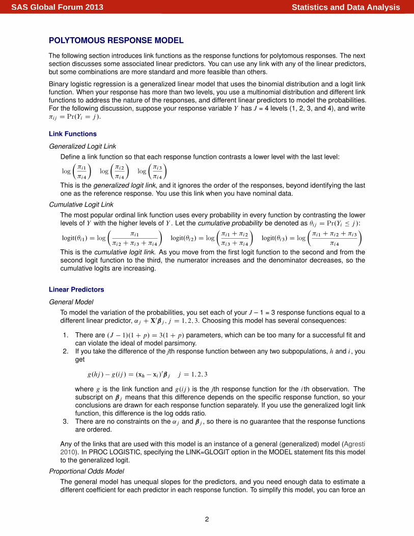
POLYTOMOUS RESPONSE MODEL

The following section introduces link functions as the response functions for polytomous responses. The nextsection discusses some associated linear predictors. You can use any link with any of the linear predictors,but some combinations are more standard and more feasible than others.

Binary logistic regression is a generalized linear model that uses the binomial distribution and a logit linkfunction. When your response has more than two levels, you use a multinomial distribution and different linkfunctions to address the nature of the responses, and different linear predictors to model the probabilities.For the following discussion, suppose your response variable Y has J = 4 levels (1, 2, 3, and 4), and write�ij D Pr.Yi D j /.

Link Functions

Generalized Logit Link

Define a link function so that each response function contrasts a lower level with the last level:

log��i1

�i4

�log

��i2

�i4

�log

��i3

�i4

�This is the generalized logit link, and it ignores the order of the responses, beyond identifying the lastone as the reference response. You use this link when you have nominal data.

Cumulative Logit Link

The most popular ordinal link function uses every probability in every function by contrasting the lowerlevels of Y with the higher levels of Y . Let the cumulative probability be denoted as �ij D Pr.Yi � j /:

logit.�i1/ D log�

�i1

�i2 C �i3 C �i4

�logit.�i2/ D log

��i1 C �i2

�i3 C �i4

�logit.�i3/ D log

��i1 C �i2 C �i3

�i4

�This is the cumulative logit link. As you move from the first logit function to the second and from thesecond logit function to the third, the numerator increases and the denominator decreases, so thecumulative logits are increasing.

Linear Predictors

General Model

To model the variation of the probabilities, you set each of your J – 1 = 3 response functions equal to adifferent linear predictor, ˛j CX0ˇj ; j D 1; 2; 3. Choosing this model has several consequences:

1. There are .J � 1/.1C p/ D 3.1C p/ parameters, which can be too many for a successful fit andcan violate the ideal of model parsimony.

2. If you take the difference of the jth response function between any two subpopulations, h and i , youget

g.hj / � g.ij / D .xh � xi /0ˇj j D 1; 2; 3

where g is the link function and g.ij / is the jth response function for the i th observation. Thesubscript on ˇj means that this difference depends on the specific response function, so yourconclusions are drawn for each response function separately. If you use the generalized logit linkfunction, this difference is the log odds ratio.

3. There are no constraints on the ˛j and ˇj , so there is no guarantee that the response functionsare ordered.

Any of the links that are used with this model is an instance of a general (generalized) model (Agresti2010). In PROC LOGISTIC, specifying the LINK=GLOGIT option in the MODEL statement fits this modelto the generalized logit.

Proportional Odds Model

The general model has unequal slopes for the predictors, and you need enough data to estimate adifferent coefficient for each predictor in each response function. To simplify this model, you can force an

2


ordering on the linear predictors by using the same slope parameters for each response function and byconstraining the intercepts to increase (˛1 < ˛2 < ˛3) or decrease:

g.j / D ˛j CX0ˇ j D 1; 2; 3

This model has J � 1C p parameters and thus requires less data for an adequate fit than the generalmodel requires. It also provides a more straightforward interpretation. Compute the difference of the jthresponse function between two subpopulations h and i to see the impact of this model:

g.hj / � g.ij / D .xh � xi /0ˇ j D 1; 2; 3

This difference is proportional to the distance between the explanatory variables, and the difference isthe same no matter which response function you consider. This is the equal slopes assumption, whichis also called the parallel lines assumption. You can apply the parallel lines assumption to any of thelink functions, but it is most commonly used with the cumulative logit link. When you use the cumulativelogit link, the assumption is the proportional odds assumption, the model is the proportional odds model,and the difference of cumulative logits (g) is the log cumulative odds ratio. By default, PROC LOGISTICfits the proportional odds model combined with the cumulative logit link when you have more than tworesponse levels.

Partial Proportional Odds Model

The third linear predictor is a hybrid of the general model and the proportional odds model. Suppose oneset of effects X has p1 parameters that satisfy the parallel lines assumption (that is, they have equalslopes), but the remaining set Z has p2 parameters that do not and instead require the general model(that is, they have unequal slopes). This model is written as

g.j / D ˛j CX0ˇ C Z0 j j D 1; 2; 3

It has .J � 1/C p1 C .J � 1/p2 parameters and, when used with the cumulative logit link, is called thepartial proportional odds model (Peterson and Harrell 1990). Interpretation of the proportional oddsparameters is independent of the response function; interpretation of the general parameters dependson the response function. When you fit the partial proportional odds model, you must be especiallycareful to ensure that the cumulative logits remain ordered for the data being modeled.

The next sections fit proportional odds models and partial proportional odds models to several data sets.

ASBESTOS DATA: PROPORTIONAL ODDS MODEL

This example fits a proportional odds model to the following Asbestos data set (Simonoff 2003, Section10.2), which can be accessed from StatLib:

data Asbestos;input Task Ventilation Exposure Freq @@;datalines;

0 0 1 29 0 0 2 1 0 0 3 1 0 1 1 3 0 1 2 1 0 1 3 21 0 1 10 1 0 2 1 1 0 3 7 1 1 1 3 1 1 2 3 1 1 3 22;

The Task variable is 0 if the worker removed asbestos tile and 1 if the worker removed asbestos insulation.The Ventilation variable is 0 if a negative pressure ventilation system was used and 1 if a general systemwas in place. The response variable Exposure measures the extent of the worker’s exposure to asbestos; ittakes the values 1 for low exposure, 2 for exposure near the legal limit, or 3 for exposure above the legallimit. The Freq variable counts the number of workers in each grouping.

The following code fits a proportional odds model to the Asbestos data set; the classification variables areentered as main effects. The CLASS statement is optional for these data, but you specify the PARAM=REFand REF=FIRST options in the CLASS statement to preserve the 0-1 coding of the two binary covariates(PARAM=REF is the incremental effects parameterization). The EFFECTPLOT statement displays a plot ofthe fit.

3


proc logistic data=Asbestos;freq Freq;class Task Ventilation / param=ref ref=first;model Exposure = Task Ventilation / aggregate scale=none;effectplot interaction(x=task plotby=ventilation sliceby=Exposure) / polybar;

run;

Because the response has more than two levels, PROC LOGISTIC by default fits cumulative logits combinedwith the proportional odds model, which has a different intercept for each response function but the sameslopes:

logit.Pr.Exposure � 1jxi / D ˛1 C .Task=1/ˇ1 C .Ventilation=1/ˇ2logit.Pr.Exposure � 2jxi / D ˛2 C .Task=1/ˇ1 C .Ventilation=1/ˇ2

This model has only four combinations of the explanatory variables, as shown in Table 1.

Table 1 Subpopulations for the Asbestos Data Set

Subpopulation Task Ventilation Description

a 0 0 Workers who removed tile with negative pressure ventilationb 1 0 Workers who removed insulation with negative pressure ventilationc 0 1 Workers who removed tile with general ventilationd 1 1 Workers who removed insulation with general ventilation

Each subpopulation has two cumulative logits in the model. If you write the cumulative probabilities for thesubpopulations in each logit function as �ij D Pr.Exposure � j jsubpopulation D i/, the model is2666666666664

logit.�a1/logit.�b1/logit.�c1/logit.�d1/

logit.�a2/logit.�b2/logit.�c2/logit.�d2/

3777777777775D

2666666666664

˛1˛1 Cˇ1˛1 Cˇ2˛1 Cˇ1 Cˇ2

˛2˛2 Cˇ1˛2 Cˇ2˛2 Cˇ1 Cˇ2

3777777777775D

2666666666664

1 0 0 0

1 0 1 0

1 0 0 1

1 0 1 1

0 1 0 0

0 1 1 0

0 1 0 1

0 1 1 1

3777777777775

2664˛1˛2ˇ1ˇ2

3775

The first row in the preceding equations shows you that the intercept for the first response function, ˛1, is thelog odds of Exposure = 1 versus 2 or 3 for Task = 0 and Ventilation = 0. The fifth row shows you that theintercept ˛2 is the log odds of Exposure = 1 or 2 versus 3 for Task = 0 and Ventilation = 0. The second (orsixth) row, compared to the first (or fifth), shows you that ˇ1 is the increment in both response functions (orboth types of log cumulative odds) due to Task = 1. The third (or seventh) row, compared to the first (or fifth),shows you that ˇ2 is the increment in both types of log cumulative odds due to Ventilation = 1.

Exponentiating the cumulative logits produces the cumulative odds, and you can solve for the cumulativeprobabilities:

logit.�j / D ˛j CX0ˇ !�j

.1 � �j /D exp.˛j CX0ˇ/! �j D exp.X0ˇ/=.1C exp.X0ˇ//

Table 2 displays these equations for each of the subpopulations and cumulative logits.

4


Table 2 Cumulative Logits, Odds, and Probabilities for the Subpopulations

Subpopulation Task Ventilation Logit Odds Probability

a 0 0 logit.�a1/ D ˛1 e˛1 e˛1=.1C e˛1/

b 1 0 logit.�b1/ D ˛1 C ˇ1 e˛1Cˇ1 e˛1Cˇ1=.1C e˛1Cˇ1/

c 0 1 logit.�c1/ D ˛1 C ˇ2 e˛1Cˇ2 e˛1Cˇ2=.1C e˛1Cˇ2/

d 1 1 logit.�d1/ D ˛1 C ˇ1 C ˇ2 e˛1Cˇ1Cˇ2 e˛1Cˇ1Cˇ2=.1C e˛1Cˇ1Cˇ2/

a 0 0 logit.�a2/ D ˛2 e˛2 e˛2=.1C e˛2/

b 1 0 logit.�b2/ D ˛2 C ˇ1 e˛2Cˇ1 e˛2Cˇ1=.1C e˛2Cˇ1/

c 0 1 logit.�c2/ D ˛2 C ˇ2 e˛2Cˇ2 e˛2Cˇ2=.1C e˛2Cˇ2/

d 1 1 logit.�d2/ D ˛2 C ˇ1 C ˇ2 e˛2Cˇ1Cˇ2 e˛2Cˇ1Cˇ2=.1C e˛2Cˇ1Cˇ2/

Figure 1 displays the response profiles. The note means that the first logit function compares Exposure = 1to Exposure = 2 or 3, and the second logit function compares Exposure = 1 or 2 to Exposure = 3; thatis, they compare lower exposure levels to higher exposure levels. You can compare higher values to lowervalues by specifying the DESCENDING response option.

Figure 1 Response Information

Response Profile

Ordered TotalValue Exposure Frequency

1 1 452 2 63 3 32

Probabilities modeled are cumulated over the lower Ordered Values.

Figure 2 displays a score test for the proportional odds assumption; the test does not reject the null hypothesisthat the proportional odds assumption holds. The degrees of freedom are the difference between the numberof parameters in a general model and the number of parameters in a proportional odds model; in this case,6 – 4 = 2. This score test actually tends to reject the null hypothesis more often than it should; Stokes,Davis, and Koch (2012) say that this statistic needs approximately five observations (or frequencies) for eachoutcome at each level of each main effect, because small samples might make the statistic artificially large.This score test is a good confirmatory test if it does not reject the null; however, if it rejects the null, then youneed other means to justify the proportional odds assumption.

Figure 2 Test for Equal Slopes Is Not Rejected

Score Test for the Proportional Odds Assumption

Chi-Square DF Pr > ChiSq

1.6130 2 0.4464

The AGGREGATE SCALE=NONE options produce the goodness-of-fit statistics that are displayed in Figure 3.These tests compare the actual number of observations in each subpopulation to the number that is predictedby the model, and both tests suggest an adequate fit. The degrees of freedom are the number of responsefunctions times the number of profiles minus the number of parameters, 4 � 2 – 4 = 4. The note in Figure 3,“Number of unique profiles: 4,” refers to the four subpopulations that are identified earlier. Stokes, Davis, andKoch (2012) suggest that you need at least five observations per subpopulation and response in order for

5


the test to be valid. If you have a continuous variable in your model, then you should not use these tests; youshould instead compare your model to a larger model and show that your model is just as good.

Figure 3 The Model Fits the Data Adequately

Deviance and Pearson Goodness-of-Fit Statistics

Criterion Value DF Value/DF Pr > ChiSq

Deviance 2.0001 4 0.5000 0.7357Pearson 1.8628 4 0.4657 0.7610

Number of unique profiles: 4

The fit statistics that are shown in Figure 4 are often used to compare nested models. The difference of the–2 Log L statistics forms the likelihood ratio statistic that is shown in Figure 5.

Figure 4 Fit Statistics

Model Fit Statistics

InterceptIntercept and

Criterion Only Covariates

AIC 151.620 107.914SC 156.457 117.590-2 Log L 147.620 99.914

The three global tests that are displayed in Figure 5 evaluate the significance of all the predictors combined.They tell you only whether the model has some significance; they don’t say anything about the effect ofindividual predictors. There are 4 parameters – 2 intercepts = 2 degrees of freedom for these tests. Alltests in Figure 5 reject the null hypothesis that the covariates are unrelated to Exposure; that is, the modelexplains a significant amount of variation in the data.

Figure 5 Tests for Parameters Being Jointly Zero Are Rejected

Testing Global Null Hypothesis: BETA=0

Test Chi-Square DF Pr > ChiSq

Likelihood Ratio 47.7055 2 <.0001Score 41.0749 2 <.0001Wald 29.3468 2 <.0001

The tests that are displayed in Figure 6 are Wald tests that the parameters in a given effect are jointly 0.Because the classification covariates are binary and are coded in the design matrix as a single column, thetests all have one degree of freedom.

6


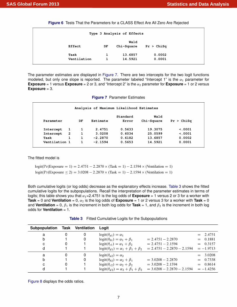
Figure 6 Tests That the Parameters for a CLASS Effect Are All Zero Are Rejected

Type 3 Analysis of Effects

WaldEffect DF Chi-Square Pr > ChiSq

Task 1 13.6857 0.0002Ventilation 1 14.5921 0.0001

The parameter estimates are displayed in Figure 7. There are two intercepts for the two logit functionsmodeled, but only one slope is reported. The parameter labeled “Intercept 1” is the ˛1 parameter forExposure = 1 versus Exposure = 2 or 3, and “Intercept 2” is the ˛2 parameter for Exposure = 1 or 2 versusExposure = 3.

Figure 7 Parameter Estimates

Analysis of Maximum Likelihood Estimates

Standard WaldParameter DF Estimate Error Chi-Square Pr > ChiSq

Intercept 1 1 2.4751 0.5633 19.3075 <.0001Intercept 2 1 3.0208 0.6034 25.0599 <.0001Task 1 1 -2.2870 0.6182 13.6857 0.0002Ventilation 1 1 -2.1594 0.5653 14.5921 0.0001

The fitted model is

logit.Pr.Exposure D 1/ D 2:4751 � 2:2870 � .Task D 1/ � 2:1594 � .Ventilation D 1/logit.Pr.Exposure � 2/ D 3:0208 � 2:2870 � .Task D 1/ � 2:1594 � .Ventilation D 1/

Both cumulative logits (or log odds) decrease as the explanatory effects increase. Table 3 shows the fittedcumulative logits for the subpopulations. Recall the interpretation of the parameter estimates in terms oflogits; this table shows you that ˛1=2.4751 is the log odds of Exposure = 1 versus 2 or 3 for a worker withTask = 0 and Ventilation = 0, ˛2 is the log odds of Exposure = 1 or 2 versus 3 for a worker with Task = 0and Ventilation = 0, ˇ1 is the increment in both log odds for Task = 1, and ˇ2 is the increment in both logodds for Ventilation = 1.

Table 3 Fitted Cumulative Logits for the Subpopulations

Subpopulation Task Ventilation Logit

a 0 0 logit.�a1/ D ˛1 D 2:4751

b 1 0 logit.�b1/ D ˛1 C ˇ1 D 2:4751 � 2:2870 D 0:1881

c 0 1 logit.�c1/ D ˛1 C ˇ2 D 2:4751 � 2:1594 D 0:3157

d 1 1 logit.�d1/ D ˛1 C ˇ1 C ˇ2 D 2:4751 � 2:2870 � 2:1594 D �1:9713

a 0 0 logit.�a2/ D ˛2 D 3:0208

b 1 0 logit.�b2/ D ˛2 C ˇ1 D 3:0208 � 2:2870 D 0:7338

c 0 1 logit.�c2/ D ˛2 C ˇ2 D 3:0208 � 2:1594 D 0:8614

d 1 1 logit.�d2/ D ˛2 C ˇ1 C ˇ2 D 3:0208 � 2:2870 � 2:1594 D �1:4256

Figure 8 displays the odds ratios.

7


Figure 8 Odds Ratios

Odds Ratio Estimates

Point 95% WaldEffect Estimate Confidence Limits

Task 1 vs 0 0.102 0.030 0.341Ventilation 1 vs 0 0.115 0.038 0.349

Note that the interpretation of the parameter estimates in Figure 7 depends on the PARAM= option, but theodds ratios in Figure 8 are independent of the PARAM= option.

The interpretation of these odds ratios is that a person who performs Task = 1 has 0.102 times the oddsof a low exposure versus a higher exposure than a person who performs Task = 0 both for Exposure = 1versus 2 or 3 and for Exposure = 1 or 2 versus 3. That is, a person who removes insulation is more likely tohave a higher exposure to asbestos than a person who removes tile. Similarly, a person who works in anenvironment that has general ventilation is more likely to have a higher exposure to asbestos than a personwho works in an environment that has negative pressure ventilation. This summary holds for both responsefunctions, because of the proportional odds assumption.

Finally, you can generate plots of the fitted model. The EFFECTPLOT statement produces the plot inFigure 9, where you can easily see that the predicted probability of a low exposure is the highest for workerswho remove tile in negative pressure ventilation, and the probability of exposure above the legal limit ishighest for workers who remove insulation in general ventilation.

Figure 9 Fitted Probabilities

COAL DATA: PROPORTIONAL ODDS MODEL

The preceding analysis uses two classification explanatory variables; the following data have a continuousexplanatory variable. The following data, from McCullagh and Nelder (1989, p. 179), contain a measure ofthe severity of pneumoconiosis (black lung disease) in coal miners and the number of years of exposure:

data Coal;input Severity $ @@;do i=1 to 8; input Exposure freq @@; lnExposure=log(Exposure); output; end;datalines;

Normal 5.8 98 15 51 21.5 34 27.5 35 33.5 32 39.5 23 46 12 51.5 4Moderate 5.8 0 15 2 21.5 6 27.5 5 33.5 10 39.5 7 46 6 51.5 2Severe 5.8 0 15 1 21.5 3 27.5 8 33.5 9 39.5 8 46 10 51.5 5;

8


The following program fits a proportional odds model to these data and displays plots of the effect ofthe lnExposure variable. By default, PROC LOGISTIC orders the response levels alphanumerically; theORDER=DATA and DESCENDING options are specified to override the default by fitting cumulative logits ofhigher versus lower severity.

You should not use the standard goodness-of-fit tests, because the lnExposure variable is continuous. Agood alternative is to compare your main-effects model to a larger one, and test whether your smaller modelis sufficient. A reasonable extension of this model is to square the continuous effect. To get this test in PROCLOGISTIC, you specify a forward selection and include your model. If the fit is good, no other effects areadded to your model, and the score test is reported in the “Residual Chi-Square Test” table.

The three EFFECTPLOT statements display the relationship of lnExposure to Severity on three differentscales: cumulative probabilities over a range of exposure levels extended by 50%, logit of cumulativeprobabilities (because the link function here is the cumulative logit link), and individual probabilities.

proc logistic data=Coal;model Severity(order=data descending)=lnExposure|lnExposure

/ selection=forward include=1 stop=2;freq freq;effectplot / noobs extend=1.5;effectplot / noobs link;effectplot / noobs individual;

run;

The proportional odds assumption is not rejected (p = 0.7103), so it is reasonable to believe that theresponse functions have a common lnExposure parameter. The global tests are all significant. The residualchi-square test for goodness of fit does not reject your model (p = 0.356), where the degrees of freedom arethe difference in the number of parameters in each of these models, df = 2 – 1 = 1.

The parameters are significant, as shown in Figure 10. Because you are fitting two response functions,you have two intercept parameters: the log odds of severe pneumoconiosis versus moderate or normalpneumoconiosis for coal miners who have no log(exposure), and the log odds of severe or moderatepneumoconiosis versus normal pneumoconiosis for coal miners who have Exposure = 1. Because of theproportional odds assumption, there is only one lnExposure parameter ˇ1, which is the increment for bothtypes of log odds due to a one-unit increment in log(exposure).



Standard WaldParameter DF Estimate Error Chi-Square Pr > ChiSq

Intercept Severe 1 -10.5817 1.3454 61.8569 <.0001Intercept Moderate 1 -9.6761 1.3241 53.4042 <.0001lnExposure 1 2.5968 0.3811 46.4299 <.0001

Figure 11 displays the odds ratios.

Figure 11 Odds Ratio for lnExposure


Point 95% WaldEffect Estimate Confidence Limits

lnExposure 13.421 6.359 28.325

9


The interpretation is that incrementing log(exposure) by 1 increases a miner’s odds of having more severepneumoconiosis by a factor of 13.

The EFFECTPLOT statements create several different views of the fitted model. First, Figure 12(A) showsthe three estimated cumulative probability functions. The plot is extended beyond the data to display theS-shaped curve of the logistic function. Because the lnExposure values are fit toward the left half of thelogit functions, the predicted probabilities of higher severity are generally quite low. Second, Figure 12(B)shows the fit on the logit scale, which has the parallel lines that you expect when making the proportionalodds assumption. Third, Figure 12(C) shows the model-predicted probabilities of a miner having each levelof Severity across the range of the lnExposure values. A miner who has little exposure has the highestprobability of being normal. As exposure increases, the higher severity levels become more likely and theprobability of a normal level decreases. When exposure exceeds 33 years, the probability of a moderateseverity levels off. Presumably miners are moving from normal to moderate severity and from moderate tosevere, so after this amount of exposure they mostly move into the severe range.

Figure 12 Displays of the Fitted Model

(A) Probability Scale (B) Logit Scale (C) Individual Probabilities

BACKACHE DATA: PROPORTIONAL ODDS MODEL

The previous examples illustrate the use of the proportional odds model when the proportional oddsassumption is satisfied. The “Backache in Pregnancy” data set from Chatfield (1995, Exercise D.2), accessedfrom StatLib, challenges those assumptions. The following data were gathered from all women who gavebirth in the London Hospital over a four-month period in 1973:

data Backache;input Severity Month Age @@;lnAge=log(Age);if Severity=0 then Severity=1;Trimester=(Month>6)+(Month>3)+1;datalines;

... more lines ...

1 0 23 3 0 36 1 0 21 1 0 30 1 0 42 1 0 34 3 3 26 1 7 18 3 6 39 1 0 25;

The variables that are extracted from this data set are Severity, which takes the values 1 = none or verylittle pain, 2 = troublesome pain, and 3 = severe pain; Trimester, which identifies in which trimester the painstarts; and lnAge, which is the log of the mother’s age in years.

The following program fits a proportional odds model to the data. The third trimester is the reference level forthe Trimester parameterization. Specifying the DESCENDING option means that the probability of higherseverity is modeled.

10


proc logistic data=Backache;class Trimester / param=ref;model Severity(descending)=lnAge Trimester;

run;

The analysis (not shown) indicates that lnAge and Trimester do indeed significantly affect Severity, but thescore test for the proportional odds assumption in Figure 13 is strongly rejected.

Figure 13 Proportional Odds Rejected!

Score Test for the Proportional Odds Assumption


22.2794 3 <.0001

As mentioned earlier, rejection tends to occur more often than it should. Now what should you do?

You can first try to determine whether the proportional odds assumption is actually valid. There are otherways to assess the proportional odds structure besides relying on this test. Two graphical methods arediscussed in the next section.

GRAPHICAL ASSESSMENT OF PROPORTIONAL ODDS

One way to judge whether the proportional odds assumption holds is to look at plots of the empiricalcumulative logit function. Recall that if you fit a proportional odds model to data, then plots of the resultingfitted cumulative logits are parallel. (See Figure 12.) Conversely, if the empirical cumulative logits lookapproximately parallel, then this provides evidence that a proportional odds model is appropriate. The%EmpiricalLogitPlot macro uses the code that is provided in SAS Note 37944 (2012) to produce empiricalcumulative logit plots. (See support.sas.com/statpapercode for this code and other code used in thispaper.) For a classification covariate A, compute the empirical cumulative logits as

log#fY � j j A D ag#fY > j j A D ag

for j D 1; 2 and a D 0; 1

To compute empirical cumulative logits for the continuous covariates, accumulate counts #fY � j g; j D 1; 2in a neighborhood of each value, use these values to compute an empirical cumulative logit, and smooth theresulting plot. The empirical cumulative logits are marginal; that is, they do not adjust for any other variablesin the model. An example of these curves for continuous variables X1 and X2 and classification variablesA and B, where both the A and X1 variables have equal slopes and the B and X2 variables have unequalslopes, is displayed in Figure 14(A). In order for the variables to satisfy the proportional odds assumption, theempirical cumulative logit curves should move in a similar fashion while holding an approximately constantdistance between them.

Harrell (2001) proposes an alternative graphical technique for assessing proportionality. He compares themean value of the predictor X within each level of the response Y to the model-expected value of X jY D j ,given that the proportional odds assumption holds for the single-effect model. Again, the effects are notadjusted for the other parameters in the model, so this provides an unadjusted check of the assumptions.The %EXPlot macro computes these statistics. An example of this plot is shown in Figure 14(B), which usesthe same variables as (A). These plots are interpreted as follows:

• To confirm the ordinality of the response for a predictor, the means should be strictly increasing ordecreasing with respect to the Y variable.

• To assess the proportional odds assumption for a predictor, the model-expected value curve shouldclosely follow the mean curve.

The macro requires CLASS variables to be numeric; otherwise, you can use the coding from the designmatrix data set that is provided by the OUTDESIGN= option in the PROC LOGISTIC statement.

11


support.sas.com/statpapercode

Figure 14 Assessment Plots (A and X1 have proportional odds)

(A) Empirical Cumulative Logits by X (B) OE.X jSeverity/ by Severity

The following code applies these macros to the Backache data set and produces Figure 15:

%EmpiricalLogitPlot(class=Trimester,cont=lnAge,data=Backache,y=Severity);%EXPlot(Trimester lnAge,data=Backache,y=Severity);

Figure 15 Assessment Plots for Backache Data

(A) Empirical Cumulative Logits by X (B) OE(X|Y) by Y

The plots for lnAge show no profound departure from proportionality (the mean curve in (B) is increasing),but the plots for Trimester certainly do show a departure. But how do you generate a model in whichthe proportional odds structure holds for one covariate but not for another? The answer is the partialproportional odds model, a hybrid method in which the lnAge variable has a proportional odds structure andthe Treatment variable has a general structure. The partial proportional odds model for the Backache datais

logit.Pr.Severity D 3// D ˛1 C .Trimester D 1/ˇ11 C .Trimester D 2/ˇ21 C lnAgeˇ3logit.Pr.Severity � 2// D ˛2 C .Trimester D 1/ˇ12 C .Trimester D 2/ˇ22 C lnAgeˇ3

where the response functions share the lnAge parameter but each function has its own version of theintercept, the Trimester = 1 parameter, and the Trimester = 2 parameter. To interpret these parameters andtheir odds ratios, the lnAge parameter is treated as before—your interpretation applies to both responsefunctions. However, when you discuss the Trimester = 1 parameter, you have to distinguish between the

12


Severity = 3 versus 2 or 1 logit function and the Severity = 3 or 2 versus 1 logit function. The partialproportional odds model is fit in the next section.

BACKACHE DATA: PARTIAL PROPORTIONAL ODDS MODEL

With SAS/STAT 12.1, you can use the LOGISTIC procedure to fit the partial proportional odds model. Thefollowing code fits this model to the Backache data; the model is specified in the same way as you wouldspecify a proportional odds model, except that you add the UNEQUALSLOPES option.

proc logistic data=Backache;class Trimester / param=ref;model Severity(descending)=lnAge Trimester / unequalslopes=Trimester;oddsratio lnAge;oddsratio Trimester;

run;

Specifying the UNEQUALSLOPES option modifies models that use the cumulative link functions. Insteadof applying the proportional odds assumption to every effect, you can apply the assumption to specificeffects. If you do not specify any effects in the UNEQUALSLOPES option, then the general model is fit tothe cumulative links. The general model has the same number of parameters that you get by specifyingLINK=GLOGIT (although the link is different). If you have a predictor that does not satisfy the proportionalodds assumption, then the UNEQUALSLOPES option enables you to fit a different parameter for everyresponse function; that is, the predictor has unequal slopes across the response functions. If you havea predictor that satisfies the proportional odds assumption, then it has equal slopes across the responsefunctions.

In this case, specifying the UNEQUALSLOPES=Trimester option creates a different parameter for eachlevel of the Trimester effect in each response function, and the proportional odds structure still holds for thelnAge variable. The ODDSRATIO statements are also specified to compute odds ratios that compare alllevels of the Trimester effect.

The global tests in Figure 16 conclude that the parameters are significantly nonzero, and the Type 3 testsshow that the group of four parameters that make up the Trimester effect (Trimester = 1 and 2 for eachresponse function) are not all 0.

Figure 16 Tests of Effect Parameters

Testing Global Null Hypothesis: BETA=0

Test Chi-Square DF Pr > ChiSq

Likelihood Ratio 44.0609 5 <.0001Score 41.5082 5 <.0001Wald 35.9914 5 <.0001

Type 3 Analysis of Effects

WaldEffect DF Chi-Square Pr > ChiSq

lnAge 1 5.0543 0.0246Trimester 4 33.7063 <.0001

As in the analysis of the Coal data set, you should not use the standard goodness-of-fit tests because thelnAge variable is continuous. Instead compare your model to a reasonable extension: in this case, takethe interaction and square the continuous effect. You can produce the Rao score test in Figure 17 from aforward selection step as shown in the following code:

13


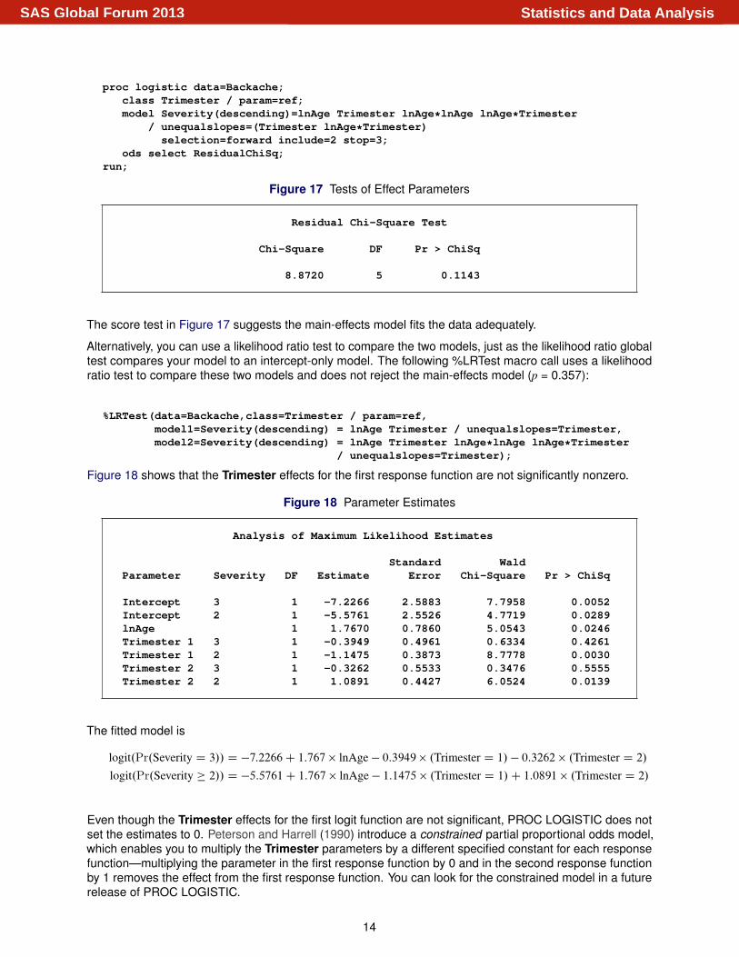
proc logistic data=Backache;class Trimester / param=ref;model Severity(descending)=lnAge Trimester lnAge*lnAge lnAge*Trimester

/ unequalslopes=(Trimester lnAge*Trimester)selection=forward include=2 stop=3;

ods select ResidualChiSq;run;

Figure 17 Tests of Effect Parameters

Residual Chi-Square Test


8.8720 5 0.1143

The score test in Figure 17 suggests the main-effects model fits the data adequately.

Alternatively, you can use a likelihood ratio test to compare the two models, just as the likelihood ratio globaltest compares your model to an intercept-only model. The following %LRTest macro call uses a likelihoodratio test to compare these two models and does not reject the main-effects model (p = 0.357):

%LRTest(data=Backache,class=Trimester / param=ref,model1=Severity(descending) = lnAge Trimester / unequalslopes=Trimester,model2=Severity(descending) = lnAge Trimester lnAge*lnAge lnAge*Trimester

/ unequalslopes=Trimester);

Figure 18 shows that the Trimester effects for the first response function are not significantly nonzero.



Standard WaldParameter Severity DF Estimate Error Chi-Square Pr > ChiSq

Intercept 3 1 -7.2266 2.5883 7.7958 0.0052Intercept 2 1 -5.5761 2.5526 4.7719 0.0289lnAge 1 1.7670 0.7860 5.0543 0.0246Trimester 1 3 1 -0.3949 0.4961 0.6334 0.4261Trimester 1 2 1 -1.1475 0.3873 8.7778 0.0030Trimester 2 3 1 -0.3262 0.5533 0.3476 0.5555Trimester 2 2 1 1.0891 0.4427 6.0524 0.0139

The fitted model is

logit.Pr.Severity D 3// D �7:2266C 1:767 � lnAge � 0:3949 � .Trimester D 1/ � 0:3262 � .Trimester D 2/logit.Pr.Severity � 2// D �5:5761C 1:767 � lnAge � 1:1475 � .Trimester D 1/C 1:0891 � .Trimester D 2/

Even though the Trimester effects for the first logit function are not significant, PROC LOGISTIC does notset the estimates to 0. Peterson and Harrell (1990) introduce a constrained partial proportional odds model,which enables you to multiply the Trimester parameters by a different specified constant for each responsefunction—multiplying the parameter in the first response function by 0 and in the second response functionby 1 removes the effect from the first response function. You can look for the constrained model in a futurerelease of PROC LOGISTIC.

14


You can interpret the intercepts and the lnAge parameter as before. The first intercept (–7.2266) is the logodds of Severity = 3 versus 2 or 1 for lnAge = 0 and Trimester = 3. The second intercept (–5.5761) is thelog odds of Severity = 3 or 2 versus 1 for lnAge = 0 and Trimester = 3. The lnAge parameter (1.767) is theincrement in log odds of a higher Severity for a one-unit increase in lnAge.

The interpretation of the Trimester parameters is complicated because they depend on the responsefunction. In the first response function, the Trimester = 1 parameter (–0.3949) is the increment in log oddsfor Severity = 3 versus 2 or 1 for pain onset in Trimester = 1, and the Trimester = 2 parameter (–0.3262) isthe increment in log odds for Severity = 3 versus 2 or 1 for pain onset in Trimester = 2. Neither of theseis significant. In the second response function, the Trimester = 1 parameter (–1.1475) is the increment inlog odds for Severity = 3 or 2 versus 1 for pain onset in Trimester = 1, and the Trimester = 2 parameter(1.0891) is the increment in log odds for Severity = 3 or 2 versus 1 for pain onset in Trimester = 2.

Similarly, the Trimester odds ratios that are displayed in Figure 19 also depend on the response functions.For the response function that compares Severity = 3 versus 2 or 1, every confidence interval contains 1, somothers who experience pain onset in any trimester are equally likely to have higher-severity pain; that is,the Trimester effect does not describe any variation in the first response function. However, in the secondresponse function, which compares Severity = 3 or 2 versus 1, mothers who experience pain onset in thefirst trimester are less likely to have higher-severity pain than mothers who experience pain onset in the latertrimesters, and mothers with pain onset in the second trimester are more likely to have higher-severity painthan mothers with pain onset in the third trimester. A mother with a one-unit increase in lnAge has 5.853times the odds of having (is more likely to have) a higher severity, for both response functions.


Odds Ratio Estimates and Wald Confidence Intervals

Label Estimate 95% Confidence Limits

lnAge 5.853 1.254 27.318Severity 3: Trimester 1 vs 2 0.934 0.334 2.611Severity 2: Trimester 1 vs 2 0.107 0.047 0.244Severity 3: Trimester 1 vs 3 0.674 0.255 1.782Severity 2: Trimester 1 vs 3 0.317 0.149 0.678Severity 3: Trimester 2 vs 3 0.722 0.244 2.135Severity 2: Trimester 2 vs 3 2.971 1.248 7.076

ALTERNATIVE METHODS TO ASSESS THE PROPORTIONAL ODDS ASSUMPTION

Although the previously discussed plots can suggest model appropriateness, performing tests gives you amore formal foundation for your model fitting. All tests of the proportionality assumption for an effect rely oncomparing a model in which that effect has a proportional odds structure to a model in which that effect doesnot. The differences in the tests are how you make adjustments for other variables in the model and whetheryou implement these tests as likelihood ratio, score, or Wald tests.

Three different ways of handling other effects in the model are as follows:

Up Start small with a proportional odds model and compare it to unequal slopes on each effect in turn(Peterson and Harrell 1990).

Down Start big with a general model and compare it to equal slopes on each effect in turn (Koch, Amara,and Singer 1985, p. 372).

OneUp Study proportionality for a series of one-effect models, for which Up and Down are equivalent(based on Harrell 2001, p. 332).

None of these types of test are perfect: Up and OneUp are apt to signal nonproportional odds too often;Down, which starts big, can require a lot of data and might be less able to detect proportional odds.

You can implement these tests in three ways:

15


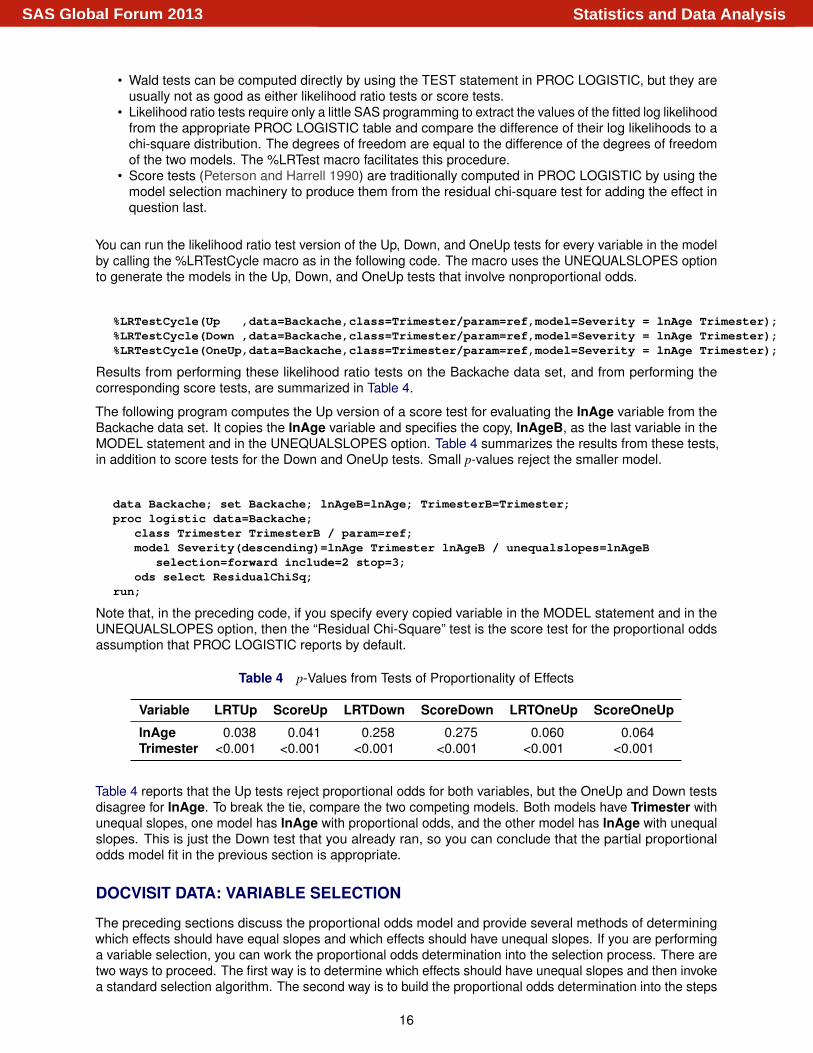
• Wald tests can be computed directly by using the TEST statement in PROC LOGISTIC, but they areusually not as good as either likelihood ratio tests or score tests.

• Likelihood ratio tests require only a little SAS programming to extract the values of the fitted log likelihoodfrom the appropriate PROC LOGISTIC table and compare the difference of their log likelihoods to achi-square distribution. The degrees of freedom are equal to the difference of the degrees of freedomof the two models. The %LRTest macro facilitates this procedure.

• Score tests (Peterson and Harrell 1990) are traditionally computed in PROC LOGISTIC by using themodel selection machinery to produce them from the residual chi-square test for adding the effect inquestion last.

You can run the likelihood ratio test version of the Up, Down, and OneUp tests for every variable in the modelby calling the %LRTestCycle macro as in the following code. The macro uses the UNEQUALSLOPES optionto generate the models in the Up, Down, and OneUp tests that involve nonproportional odds.

%LRTestCycle(Up ,data=Backache,class=Trimester/param=ref,model=Severity = lnAge Trimester);%LRTestCycle(Down ,data=Backache,class=Trimester/param=ref,model=Severity = lnAge Trimester);%LRTestCycle(OneUp,data=Backache,class=Trimester/param=ref,model=Severity = lnAge Trimester);

Results from performing these likelihood ratio tests on the Backache data set, and from performing thecorresponding score tests, are summarized in Table 4.

The following program computes the Up version of a score test for evaluating the lnAge variable from theBackache data set. It copies the lnAge variable and specifies the copy, lnAgeB, as the last variable in theMODEL statement and in the UNEQUALSLOPES option. Table 4 summarizes the results from these tests,in addition to score tests for the Down and OneUp tests. Small p-values reject the smaller model.

data Backache; set Backache; lnAgeB=lnAge; TrimesterB=Trimester;proc logistic data=Backache;

class Trimester TrimesterB / param=ref;model Severity(descending)=lnAge Trimester lnAgeB / unequalslopes=lnAgeB

selection=forward include=2 stop=3;ods select ResidualChiSq;

run;

Note that, in the preceding code, if you specify every copied variable in the MODEL statement and in theUNEQUALSLOPES option, then the “Residual Chi-Square” test is the score test for the proportional oddsassumption that PROC LOGISTIC reports by default.

Table 4 p-Values from Tests of Proportionality of Effects

Variable LRTUp ScoreUp LRTDown ScoreDown LRTOneUp ScoreOneUp

lnAge 0.038 0.041 0.258 0.275 0.060 0.064Trimester <0.001 <0.001 <0.001 <0.001 <0.001 <0.001

Table 4 reports that the Up tests reject proportional odds for both variables, but the OneUp and Down testsdisagree for lnAge. To break the tie, compare the two competing models. Both models have Trimester withunequal slopes, one model has lnAge with proportional odds, and the other model has lnAge with unequalslopes. This is just the Down test that you already ran, so you can conclude that the partial proportionalodds model fit in the previous section is appropriate.

DOCVISIT DATA: VARIABLE SELECTION

The preceding sections discuss the proportional odds model and provide several methods of determiningwhich effects should have equal slopes and which effects should have unequal slopes. If you are performinga variable selection, you can work the proportional odds determination into the selection process. There aretwo ways to proceed. The first way is to determine which effects should have unequal slopes and then invokea standard selection algorithm. The second way is to build the proportional odds determination into the steps

16


of the selection algorithm. The following sections discuss these two approaches by using the Docvisit dataset (Cameron and Trivedi 1998, p. 68) from Example 54.17 of the PROC LOGISTIC documentation in theSAS/STAT 12.1 User’s Guide.

data Docvisit;input Sex Age Agesq Income Levyplus Freepoor Freerepa

Illness Actdays Hscore Chcond1 Chcond2 Dvisits;if ( Dvisits > 2) then Dvisits = 2;Dvisitsp1= Dvisits+1;

datalines;1 0.19 0.0361 0.55 1 0 0 1 4 1 0 0 1

... more lines ...

0 0.72 0.5184 0.25 0 0 1 0 0 0 0 0 0;

The dependent variable, Dvisits, contains the number of doctor visits in the past two weeks (0, 1, or 2,where 2 represents two or more visits). Details about the other variables in the data set can be found in thePROC LOGISTIC documentation.

Proportional Odds Determination Followed by Stepwise Selection

In this section, you determine which effects should have unequal slopes before invoking the usual stepwiseselection method. For the determination of unequal slopes, you can use the plots and the likelihood ratiotests that are described earlier.

First, create the two graphical assessment plots discussed earlier and see what they suggest. The macrosrequire the response variable to take the values 1, 2, 3,..., so the Dvisitsp1 variable is used. Because allthe continuous variables take only a small number of distinct values, every variable is listed in the CLASS=option of the %EmpiricalLogitPlot macro. The following code creates the plots in Figure 20:

%EmpiricalLogitPlot(data=Docvisit,y=Dvisitsp1,class=Sex Age Agesq IncomeLevyplus Freepoor Freerepa Illness Actdays Hscore Chcond1 Chcond2);

%EXPlot(Sex Age Agesq Income Levyplus Freepoor Freerepa IllnessActdays Hscore Chcond1 Chcond2,data=Docvisit,y=Dvisitsp1);

Figure 20 Assessment Plots for Docvisit Data

(A) Empirical Cumulative Logits by X (B) OE.X jY / by Y

The empirical cumulative logits in Figure 20(A) suggest that Actdays and Income should have unequalslopes, whereas Age, Agesq, and Hscore might have unequal slopes. The OE.X jY / plots in Figure 20(B)show that the non-ordinality of the Levyplus and Chcond1 mean curves gives them unequal slopes. Theslight non-ordinality of the Age, Agesq, Freerepa, and Sex mean curves and their slight divergence fromthe expected curves suggest they might have unequal slopes. Finally, choose effects that either plot is sure

17


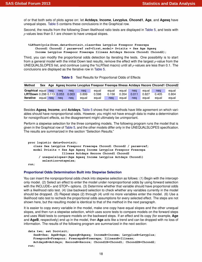
of or that both sets of plots agree on: let Actdays, Income, Levyplus, Chcond1, Age, and Agesq haveunequal slopes. Table 5 contains these conclusions in the Graphical row.

Second, the results from the following Down likelihood ratio tests are displayed in Table 5, and tests withp-values less than 0.1 are chosen to have unequal slopes.

%LRTestCycle(Down,data=Docvisit,class=Sex Levyplus Freepoor FreerepaChcond1 Chcond2 / param=ref ref=first,model= Dvisits = Sex Age AgesqIncome Levyplus Freepoor Freerepa Illness Actdays Hscore Chcond1 Chcond2);

Third, you can modify the proportional odds detection by iterating the tests. One possibility is to startfrom a general model with the initial Down test results, remove the effect with the largest p-value from theUNEQUALSLOPES list, and continue (using the %LRTest macro) until all p-values are less than 0.1. Theconclusions are displayed as the Iterative row in Table 5.

Table 5 Test Results for Proportional Odds of Effects

Method Sex Age Agesq Income Levyplus Freepoor Freerepa Illness Actdays Hscore Chcond1 Chcond2

Graphical equal neq neq neq neq equal equal equal neq equal neq equalLRTDown 0.298 0.113 0.053 0.003 0.899 0.598 0.158 0.354 0.011 0.827 0.405 0.804Iterative equal neq neq neq equal equal neq equal neq equal equal equal

Besides Agesq, Income, and Actdays, Table 5 shows that the methods have little agreement on which vari-ables should have nonproportional odds. However, you might not have enough data to make a determinationfor nonsignificant effects, so the disagreement might ultimately be unimportant.

Perform a stepwise selection for the three competing models. The following program runs the model that isgiven in the Graphical row of Table 5, and the other models differ only in the UNEQUALSLOPES specification.The results are summarized in the section “Selection Results.”

proc logistic data=Docvisit;class Sex Levyplus Freepoor Freerepa Chcond1 Chcond2 / param=ref;model Dvisits = Sex Age Agesq Income Levyplus Freepoor Freerepa

Illness Actdays Hscore Chcond1 Chcond2/ unequalslopes=(Age Agesq Income Levyplus Actdays Chcond1)

selection=stepwise;run;

Proportional Odds Determination Built into Stepwise Selection

You can insert the nonproportional odds check into stepwise selection as follows: (1) Begin with the intercept-only model. (2) Select an effect to enter the model under nonproportional odds by using forward selectionwith the INCLUDE= and STOP= options. (3) Determine whether that variable should have proportional oddswith a likelihood ratio test. (4) Use backward selection to check whether any variables currently in the modelshould be dropped. (5) Repeat steps (2) through (4) until no more variables enter the model. (6) Use alikelihood ratio test to recheck the proportional odds assumptions for every selected effect. The steps are notshown here, but the resulting model is identical to that of the method in the next paragraph.

It is easier to copy every variable in the model, make one copy have equal slopes and the other unequalslopes, and then run a stepwise selection, which uses score tests to compare models on the forward stepsand uses Wald tests to compare models on the backward steps. If an effect and its copy (for example, Ageand AgeB, respectively) end up in the model, then Age acts like a trend and can be dropped with no loss ofinformation. The results of the following program are summarized in the next section:

data two; set Docvisit;SexB=Sex; AgeB=Age; AgesqB=Agesq; IncomeB=Income; LevyplusB=Levyplus;FreepoorB=Freepoor; FreerepaB=Freerepa; IllnessB=Illness;ActdaysB=Actdays; HscoreB=Hscore; Chcond1B=Chcond1; Chcond2B=Chcond2;

run;

18


proc logistic data=two;class Sex Levyplus Freepoor Freerepa Chcond1 Chcond2 SexB LevyplusB

FreepoorB FreerepaB Chcond1B Chcond2B / param=ref ref=first;model Dvisits = Sex Age Agesq Income Levyplus Freepoor Freerepa Illness

Actdays Hscore Chcond1 Chcond2 SexB AgeB AgesqB IncomeB LevyplusBFreepoorB FreerepaB IllnessB ActdaysB HscoreB Chcond1B Chcond2B /unequalslopes=(SexB AgeB AgesqB IncomeB LevyplusB FreepoorB FreerepaB

IllnessB ActdaysB HscoreB Chcond1B Chcond2B)selection=stepwise details;

run;

Selection Results

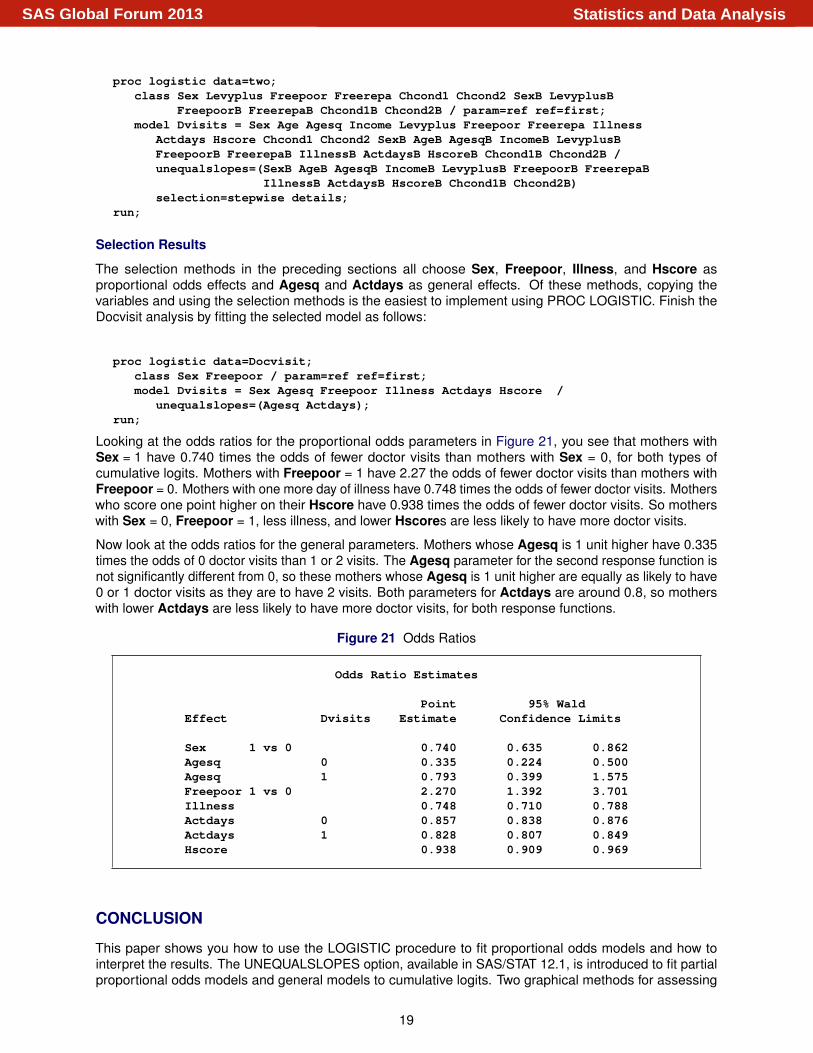
The selection methods in the preceding sections all choose Sex, Freepoor, Illness, and Hscore asproportional odds effects and Agesq and Actdays as general effects. Of these methods, copying thevariables and using the selection methods is the easiest to implement using PROC LOGISTIC. Finish theDocvisit analysis by fitting the selected model as follows:

proc logistic data=Docvisit;class Sex Freepoor / param=ref ref=first;model Dvisits = Sex Agesq Freepoor Illness Actdays Hscore /

unequalslopes=(Agesq Actdays);run;

Looking at the odds ratios for the proportional odds parameters in Figure 21, you see that mothers withSex = 1 have 0.740 times the odds of fewer doctor visits than mothers with Sex = 0, for both types ofcumulative logits. Mothers with Freepoor = 1 have 2.27 the odds of fewer doctor visits than mothers withFreepoor = 0. Mothers with one more day of illness have 0.748 times the odds of fewer doctor visits. Motherswho score one point higher on their Hscore have 0.938 times the odds of fewer doctor visits. So motherswith Sex = 0, Freepoor = 1, less illness, and lower Hscores are less likely to have more doctor visits.

Now look at the odds ratios for the general parameters. Mothers whose Agesq is 1 unit higher have 0.335times the odds of 0 doctor visits than 1 or 2 visits. The Agesq parameter for the second response function isnot significantly different from 0, so these mothers whose Agesq is 1 unit higher are equally as likely to have0 or 1 doctor visits as they are to have 2 visits. Both parameters for Actdays are around 0.8, so motherswith lower Actdays are less likely to have more doctor visits, for both response functions.



Point 95% WaldEffect Dvisits Estimate Confidence Limits

Sex 1 vs 0 0.740 0.635 0.862Agesq 0 0.335 0.224 0.500Agesq 1 0.793 0.399 1.575Freepoor 1 vs 0 2.270 1.392 3.701Illness 0.748 0.710 0.788Actdays 0 0.857 0.838 0.876Actdays 1 0.828 0.807 0.849Hscore 0.938 0.909 0.969

CONCLUSION

This paper shows you how to use the LOGISTIC procedure to fit proportional odds models and how tointerpret the results. The UNEQUALSLOPES option, available in SAS/STAT 12.1, is introduced to fit partialproportional odds models and general models to cumulative logits. Two graphical methods for assessing

19


proportionality are discussed. The UNEQUALSLOPES option also enables you to determine which variablessatisfy the proportional odds assumptions and which do not.

Expanding the scope of the LOGISTIC procedure is an active area of SAS/STAT development. You can lookfor the following features in a future release of PROC LOGISTIC: enabling effects to have both general andproportional odds structures, fitting the unconstrained partial proportional odds model, fitting generalizedlogit links with proportional odds and partial proportional odds models, and providing alternative ordinal linkssuch as the adjacent-category logit.

REFERENCES

Agresti, A. (2010), Analysis of Ordinal Categorical Data, 2nd Edition, New York: John Wiley & Sons.

Cameron, A. C. and Trivedi, P. K. (1998), Regression Analysis of Count Data, Cambridge: CambridgeUniversity Press.

Chatfield, C. (1995), Problem Solving: A Statistician’s Guide, 2nd Edition, Boca Raton, FL: Chapman &Hall/CRC.

Harrell, F. E. (2001), Regression Modeling Strategies, New York: Springer-Verlag.

Koch, G. G., Amara, I. A., and Singer, J. M. (1985), “A Two-Stage Procedure for the Analysis of OrdinalCategorical Data,” in P. K. Sen, ed., Biostatistics: Statistics in Biomedical, Public Health, and EnvironmentalSciences, Amsterdam: Elsevier Science.

McCullagh, P. and Nelder, J. A. (1989), Generalized Linear Models, 2nd Edition, London: Chapman & Hall.

Peduzzi, P., Concato, J., Kemper, E., Holford, T. R., and Feinstein, A. R. (1996), “A Simulation Study of theNumber of Events per Variable in Logistic Regression Analysis,” Journal of Clinical Epidemiology, 49,1373–1379.

Peterson, B. L. and Harrell, F. E. (1990), “Partial Proportional Odds Models for Ordinal Response Variables,”Journal of the Royal Statistical Society, Series B, 39, 205–217.

SAS Institute Inc. (2012), “SAS Note 37944: Plots to Assess the Proportional Odds Assumption in an OrdinalLogistic Model,” http://support.sas.com/kb/37944.

Simonoff, J. S. (2003), Analyzing Categorical Data, New York: Springer-Verlag.

Stokes, M. E., Davis, C. S., and Koch, G. G. (2012), Categorical Data Analysis Using SAS, 3rd Edition, Cary,NC: SAS Institute Inc.

ACKNOWLEDGMENTS

The author is grateful to Maura Stokes, Randy Tobias, David Schlotzhauer, Ed Huddleston, Anne Baxter,and Tim Arnold of the Advanced Analytics Division at SAS Institute Inc. for their valuable assistance in thepreparation of this paper.

CONTACT INFORMATION

Your comments and questions are valued and encouraged. Contact the author:

Bob DerrSAS Institute Inc.SAS Campus DriveCary, NC [email protected]

SAS and all other SAS Institute Inc. product or service names are registered trademarks or trademarks ofSAS Institute Inc. in the USA and other countries. ® indicates USA registration.

Other brand and product names are trademarks of their respective companies.

20


http://support.sas.com/kb/37944

446-2013: Ordinal Response Modeling with the LOGISTIC ... · Paper 446-2013 Ordinal Response...

Documents

Transcript of 446-2013: Ordinal Response Modeling with the LOGISTIC ... · Paper 446-2013 Ordinal Response...