Ordinal Logistic Regression

Read the data use http://www.ats.ucla.edu/stat/stata/dae/olo

git.dta, clear

Describe the data Codebook Summarize Tabulate Make graphs

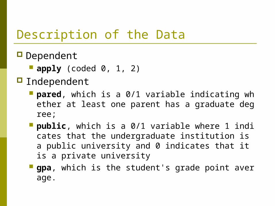
Description of the Data

Dependent apply (coded 0, 1, 2)

Independent pared, which is a 0/1 variable indicating whether

at least one parent has a graduate degree; public, which is a 0/1 variable where 1 indicates t

hat the undergraduate institution is a public university and 0 indicates that it is a private university

gpa, which is the student's grade point average.

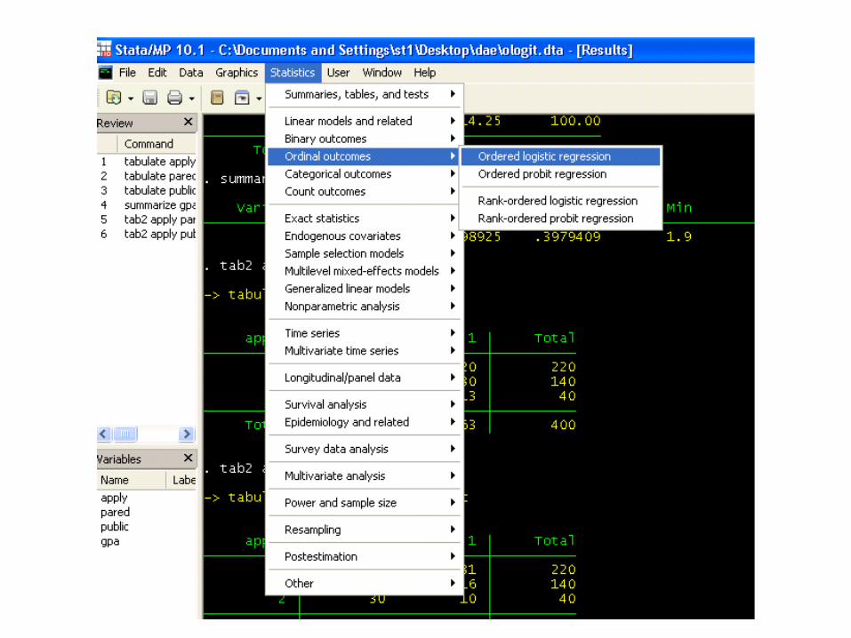
Using the Ordinal Logistic Model

Before we run our ordinal logistic model, we will see if any cells (created by the crosstab of our categorical and response variables) are empty or extremely small.  

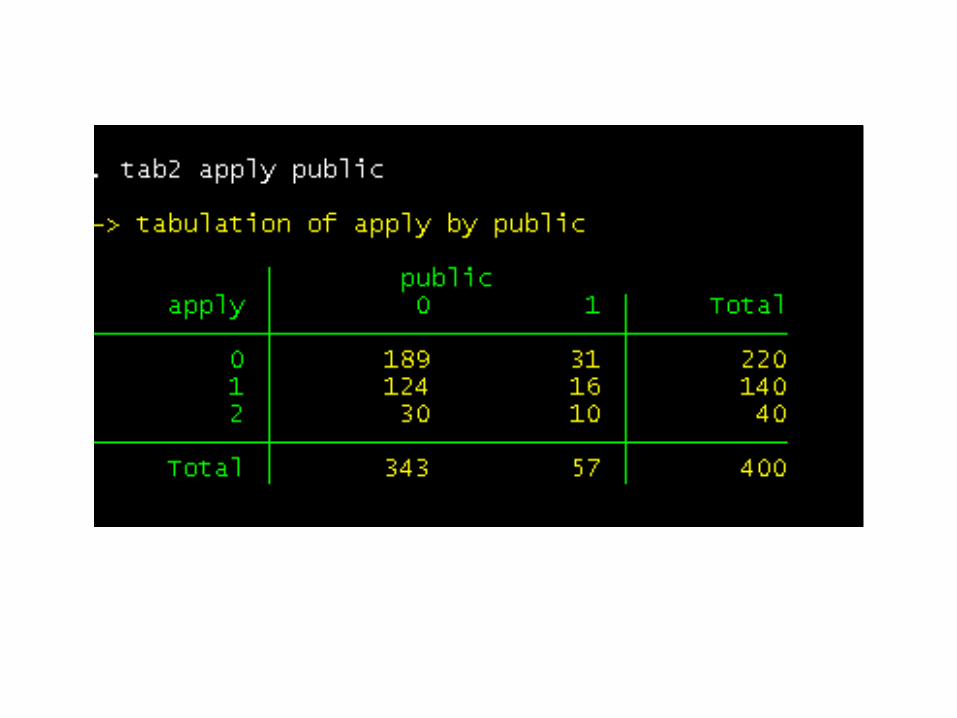
None of the cells is too small or empty (has no cases), so we will run our model.

Log likelihood (-358.51244) can be used in comparisons of nested models,

but we won't show an example of that here.  Observations (400)

Fewer observations would have been used if any of our variables had missing values. 

Likelihood ratio chi-square (24.18) our model as a whole is statistically significant,

as compared to model with no predictors.  Pseudo-R-squared

Coefficients Both pared and gpa are statistically significant; p

ublic is not.

We can obtain odds ratios using the or option after the ologit command.

For pared, we would say that for a one unit increase in pared, i.e., going from 0 to 1, the odds of high apply versus the combined middle and low categories are 2.85 greater, given that all of the other variables in the model are held constant.

For a one unit increase in gpa, the odds of the low and middle categories of apply versus the high category of apply are 1.85 times greater, given that the other variables in the model are held constant.

Because of the proportional odds assumption, the same increase, 1.85 times, is found between low apply and the combined categories of middle and high apply.

You can also use the listcoeff command to obtain the odds ratios, as well as the change in the odds for a standard deviation of the variable.

You can use the percent option to see the percent change in the odds.

Proportional Odds Assumption Ordinal logistic regression assumes that the

coefficients that describe the relationship between, say, the lowest versus all higher categories of the response variable are the same as those that describe the relationship between the next lowest category and all higher categories, etc.  This is called the proportional odds assumption or the parallel regression assumption. 

Because the relationship between all pairs of groups is the same, there is only one set of coefficients (only one model).  If this was not the case, we would need different models to describe the relationship between each pair of outcome groups. 

Test Proportional Odds Assumption

We need to download a user-written command called omodel (type findit omodel). The first test that we will show does a likelihood ratio test. The null hypothesis is that there is no difference in the coefficients between models, so we "hope" to get a non-significant result.

The brant command performs a Brant test. As the note at the bottom of the output indicates, we also "hope" that these tests are non-significant.

Both of the above tests indicate that we have not violated the proportional odds assumption. If we had, we would want to run our model as a generalized ordered logistic model using gologit2. You need to download gologit2 by typing findit gologit2.

Predicted Probability

Use pared as an example with a categorical predictor.

The predicted probability of  being in the lowest category of apply is 0.59 if neither parent has a graduate level education and 0.34 otherwise. 

For the middle category of apply, the predicted probabilities are 0.33 and 0.46, and for the highest category of apply, 0.079 and 0.196. 

Beneath each output, we can see the values at which the variables are held; by default, they are held at their mean.

The predicted probabilities for gpa at 2, 3 and 4.

The highest predicted probability is for the lowest category of apply, which makes sense because most respondents are in that category.

You can also see that the predicted probability increases for both the middle and highest categories of apply as gpa increases.

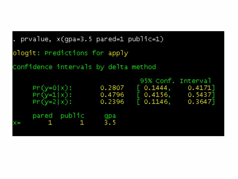
Below, we use the prvalue command to set the values of all of our predictor variables. This is useful when you want to describe profiles of respondents.