4 Pendulum analysis

On first sight, a pendulum seems simple: most people who have studied Physics know that

its period is given by T = 2πp

L/g. But when we look more closely, it is much more

complex. First there is the fairly standard adjustment for non-linearity, which means the

period increases as the amplitude of the swing increases. The amplitude in turn depends on

the energy dissipated in drag, and so varies with air density. The pendulum is temperature-

compensated, which tries to ensure its length is unchanged by thermal expansion; but there

are time delays involved which mean transient temperature changes cause the clock to gain

or loose time.

The results of these effects can be predicted, and then demonstrated in the recorded

data, which is very satisfactory. However, there are more effects that can be predicted

from a theoretic starting point (such as tidal variations in gravity) which have not yet been

detected in the data. On the other hand there are also events in the data which are yet to

be explained.

This section presents the theoretic relationships governing the clock, while the next

section presents examples of the recorded data which demonstrate these, and other, effects.

The emphasis is on the type of relationship that results, rather than the precise values

involved.

4.1 The non-linear pendulum

The equation of motion of a pendulum (Figure 4.1) is

mLθ̈ =−mg sinθ

For small oscillations, sinθ ≈ θ , so the equation of motion is linearised to θ̈ + (g/L)θ = 0.

This is standard simple harmonic motion, with period Ts = 2πp

L/g.

When the amplitude of the pendulum A is not negligible, the period is modified, as

derived in Appendix B, to be

T ≈ Ts

�

1+A2

16

�

= 2π

r

L

g

�

1+A2

16

�

(4.1)

θ

mg

Lθ̈

L

FIGURE 4.1: A simple pendulum

14

So there are three quantities which affect the period of a pendulum: amplitude, length,

and gravity. In the following sections effects which change these quantities will be consid-

ered in turn.

4.1.1 Definition of going

In general, we are ultimately most interested in the effect on the clock’s going (i.e. seconds

gained per second), which is related to pendulum period by

G =T0− T

T0=

T0− (T0+∆T )T0

=−∆T

T0(4.2)

anddG

dT=−1

T0(4.3)

The period T is very close to the nominal period T0 = 3 seconds, so T and T0 may be used

interchangeably in this context. Going is usually given in units of milliseconds per day, with

100 ms/day= 1.16 ppm.

4.2 Basic relationships

The expression for the period of a pendulum (4.1) leads directly to relationships between

going, amplitude and length.

If the pendulum has amplitude A, and using the fact that the difference between T & Ts

is 4th-order in A and hence negligible,

G =−∆T

T≈−∆T

Ts=

A2

16(4.4)

=⇒dG

dA= −

A

8(4.5)

Taking the reference amplitude as A0 = 54 mrad, this gives dG/dA=−583 (ms/day)/mrad.

Since amplitude is measured directly (unlike length and gravity), this can be directly ob-

served in the data: see Section 6.1.

Similar relationships for L and g will be useful later. Consider the effect of a change in

length ∆L:

T +∆T = 2π

r

L+∆L

g≈ 2π

r

L

g

�

1+1

2·∆L

L

�

=⇒∆T

T=

1

2·∆L

L

Similarly, ∆T/T = (−1/2)∆g/g. The following sections discuss physical effects which

influence going via these relationships.

15

PENDULUM

WEIGHTS

FIGURE 4.2: The regulation weights. The brass weights at the bottom of the stack are calibrated;the washers on top are compensating for a mysterious event on 16 April (Section 6.4).

m

M

x

L

FIGURE 4.3: Simple pendulum with an added weight.

4.3 Mass distribution (regulation)

The clock keeper must be able to adjust the running of the clock, and this is done by adding

and removing small weights on a platform halfway down the pendulum (Figure 4.2). The

effect of these weights is as follows.

A simple pendulum is shown in Figure 4.3, of length L and bob mass M , with a small

mass m added a distance x below the pivot. The kinetic and potential energies are:

T = 12mx2θ̇ 2+ 1

2M L2θ̇ 2

V ≈ mg x · θ2

2+M g L · θ

2

2

(assuming θ is small, so cosθ ≈ 1− θ2

2), so the natural frequency is

ω2 =V

T ?=

g(mx +M L)mx2+M L2

Putting ω20 = g/L gives

�

ω

ω0

�2

=mx +M L

mx2/L+M L=

1+ mxM L

1+ mx2

mL2

≈ 1+mx

M L−

mx2

mL2 (4.6)

16

The period is T = 2π/ω, so

∆T

T0=

2π/ω− 2π/ω0

2π/ω0=ω0

ω− 1

which gives (using (4.6) and the binomial expansion)

∆T

T0≈�

1−1

2

�

mx

mL−

mx2

mL2

��

− 1

=−m

2M·

x

L

�

1−x

L

�

0 0.5 1

0.25

x/L

f�

xL

�

= xL

�

1− xL

�

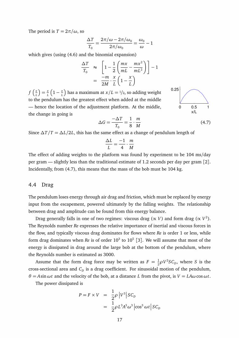
has a maximum at x/L = 1/2, so adding weight

to the pendulum has the greatest effect when added at the middle

— hence the location of the adjustment platform. At the middle,

the change in going is

∆G =−∆T

T0=

1

8·

m

M(4.7)

Since ∆T/T =∆L/2L, this has the same effect as a change of pendulum length of

∆L

L=−1

4·

m

M

The effect of adding weights to the platform was found by experiment to be 104 ms/day

per gram — slightly less than the traditional estimate of 1.2 seconds per day per gram [2].Incidentally, from (4.7), this means that the mass of the bob must be 104 kg.

4.4 Drag

The pendulum loses energy through air drag and friction, which must be replaced by energy

input from the escapement, powered ultimately by the falling weights. The relationship

between drag and amplitude can be found from this energy balance.

Drag generally falls in one of two regimes: viscous drag (∝ V ) and form drag (∝ V 2).

The Reynolds number Re expresses the relative importance of inertial and viscous forces in

the flow, and typically viscous drag dominates for flows where Re is order 1 or less, while

form drag dominates when Re is of order 103 to 105 [3]. We will assume that most of the

energy is dissipated in drag around the large bob at the bottom of the pendulum, where

the Reynolds number is estimated as 3000.

Assume that the form drag force may be written as F = 12ρV 2SCD, where S is the

cross-sectional area and CD is a drag coefficient. For sinusoidal motion of the pendulum,

θ = Asinωt and the velocity of the bob, at a distance L from the pivot, is V = LAω cosωt.

The power dissipated is

P = F × V =1

2ρ�

�V 3�

�SCD

=1

2ρL3A3ω3

�

�cos3ωt�

�SCD

17

The mean power loss is given by

P =1

2ρL3A3ω3SCD ·

1

T

Tˆ

0

�

�cos3ωt�

� d t

= kρL3A3ω3

where k is a constant, dependant on the geometry of the pendulum. This drag loss is

balanced by energy input into the pendulum by the escapement, which is in the form of

discrete ‘kicks’, so it is reasonable to assume that the energy per cycle is constant, i.e.

P̄ T = 2πP̄/ω= const. So

ρL3A3ω2 = const (4.8)

We can derive several results from this, by varying either air density or pendulum length.

4.4.1 Changes in air density

What is the variation in amplitude caused by a change in air density? We know (from

Appendix B) that ω2 = ω20(1− A2/8). Assuming length L remains constant, substituting

this into (4.8) gives

ρA3

�

1−A2

8

�

≈ ρA3 = const

∴dA

dρ=−A

3ρ

At a typical amplitude of 54 milliradians and with a typical air density of 1.2 kgm−3, this

gives dA/dρ =−15mrad/kgm−3. Combining this with dG/dA from (4.5) we get

dG

dρ=

dG

dA×

dA

dρ=�−A

8

�

×�−A

3ρ

�

=A2

24ρ= 8700 msday−1/kgm−3

4.4.2 Changes in length

If instead length varies and density is held constant, substituting ω2 = g/L into (4.8) gives

L2A3 = const

∴dA

dL=−2A

3L

Alternatively, eliminating L using L3 = g/ω6 gives

A3ω−4 = C1 =⇒ A3T 4 = C2

∴dT

dA=−3T

4A=⇒

dG

dA=−3

4A

18

R

T1

T2

α

T0 0 2 4 6

0

2

4

6

∆T

Tem

p, change / d

egre

es

Time / hours

ambient

inner

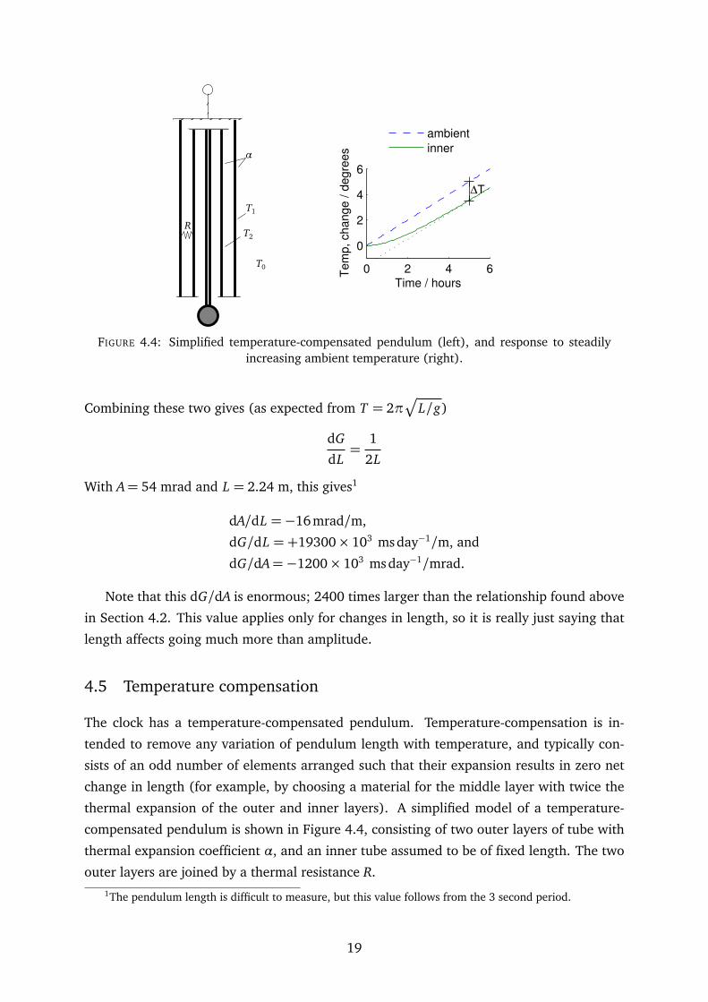
FIGURE 4.4: Simplified temperature-compensated pendulum (left), and response to steadilyincreasing ambient temperature (right).

Combining these two gives (as expected from T = 2πp

L/g)

dG

dL=

1

2L

With A= 54 mrad and L = 2.24 m, this gives1

dA/dL =−16mrad/m,

dG/dL =+19300× 103 ms day−1/m, and

dG/dA=−1200× 103 ms day−1/mrad.

Note that this dG/dA is enormous; 2400 times larger than the relationship found above

in Section 4.2. This value applies only for changes in length, so it is really just saying that

length affects going much more than amplitude.

4.5 Temperature compensation

The clock has a temperature-compensated pendulum. Temperature-compensation is in-

tended to remove any variation of pendulum length with temperature, and typically con-

sists of an odd number of elements arranged such that their expansion results in zero net

change in length (for example, by choosing a material for the middle layer with twice the

thermal expansion of the outer and inner layers). A simplified model of a temperature-

compensated pendulum is shown in Figure 4.4, consisting of two outer layers of tube with

thermal expansion coefficient α, and an inner tube assumed to be of fixed length. The two

outer layers are joined by a thermal resistance R.1The pendulum length is difficult to measure, but this value follows from the 3 second period.

19

The change of length of the pendulum due to thermal expansion is

∆L = αL(T1− T2)

and the going resulting from this is

∆G =−∆T

T=−1

2·∆L

L=−α2(T1− T2)

In steady state, the temperature will be uniform throughout the pendulum and it will

be at its design length. The behaviour gets more interesting when the ambient temperature

is changing. For example, Appendix C derives the response to a steadily increasing ambi-

ent temperature: a steady temperature difference will develop between the layers of the

pendulum, which remains as long as the ambient temperature keeps increasing. The size

of this temperature difference is, from the Appendix,

T1− T2 = τdT1

d t

This causes a change in going of

∆G =−ατ

2·

dT1

d t=−k

dT1

d twhere, making various assumptions about heat transfer and capacity, k is estimated as

40 ms/degree. Since G = G0−k dT1

d t, where G0 should ideally be zero if the correct regulation

weights have been used, the drift should vary as

D =ˆ

G dt =−kT1+ G0 t + const

i.e. drift is proportional to temperature.

The system has a time constant, which is estimated as τ≈ 1.5 hours. These results will

only hold once the temperature difference has built up, after a few time constants (perhaps

3 hours). So, we should expect to see a variation in drift due to diurnal temperature

changes, and also due to longer-term seasonal changes.

4.6 Changes in gravity

So far, looking at the expression for period

T = 2π

r

L

g

�

1+A2

16

�

we have considered the effect of changes in amplitude A and length L. The remaining

variation to consider is changes in gravity g. There are three main influences on this: the

Moon and the Sun’s varying gravitational pull, which actually changes g; and buoyancy

forces and the added inertia of entrained air, which effectively decrease g.

20

0 1 2 3 4 5 6 7 8 9 10 11 12 13 14 15−2.5

−2.45

−2.4

−2.35

−2.3

−2.25

−2.2V

ariation in "

g"

/ ppm

Days from New Moon

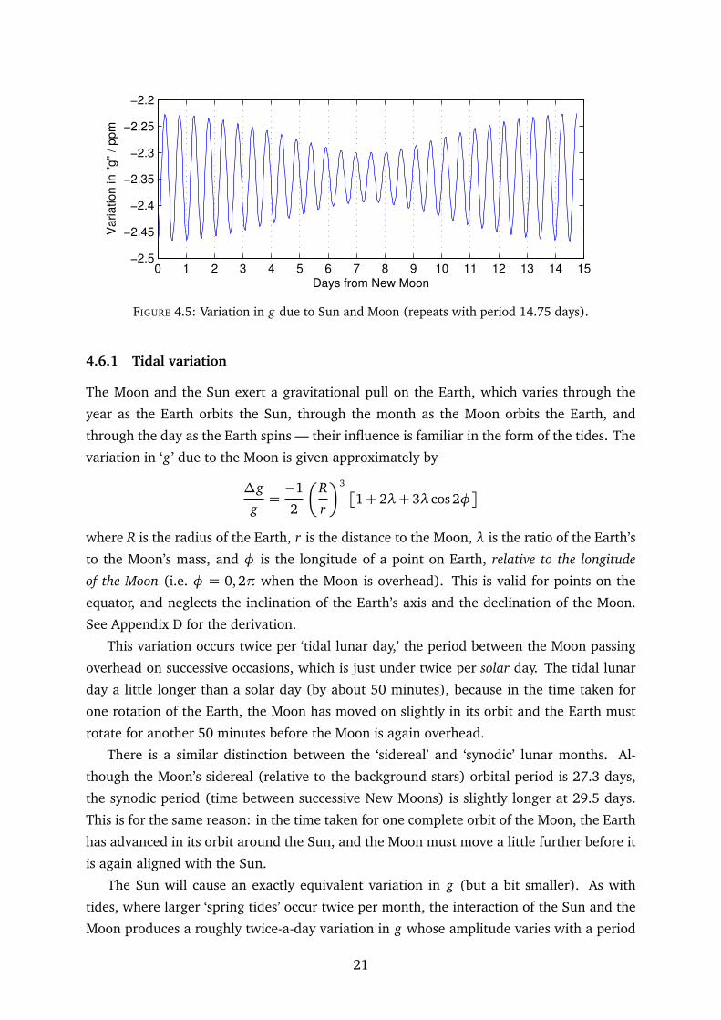
FIGURE 4.5: Variation in g due to Sun and Moon (repeats with period 14.75 days).

4.6.1 Tidal variation

The Moon and the Sun exert a gravitational pull on the Earth, which varies through the

year as the Earth orbits the Sun, through the month as the Moon orbits the Earth, and

through the day as the Earth spins — their influence is familiar in the form of the tides. The

variation in ‘g ’ due to the Moon is given approximately by

∆g

g=−1

2

�

R

r

�3�

1+ 2λ+ 3λ cos 2φ�

where R is the radius of the Earth, r is the distance to the Moon, λ is the ratio of the Earth’s

to the Moon’s mass, and φ is the longitude of a point on Earth, relative to the longitude

of the Moon (i.e. φ = 0,2π when the Moon is overhead). This is valid for points on the

equator, and neglects the inclination of the Earth’s axis and the declination of the Moon.

See Appendix D for the derivation.

This variation occurs twice per ‘tidal lunar day,’ the period between the Moon passing

overhead on successive occasions, which is just under twice per solar day. The tidal lunar

day a little longer than a solar day (by about 50 minutes), because in the time taken for

one rotation of the Earth, the Moon has moved on slightly in its orbit and the Earth must

rotate for another 50 minutes before the Moon is again overhead.

There is a similar distinction between the ‘sidereal’ and ‘synodic’ lunar months. Al-

though the Moon’s sidereal (relative to the background stars) orbital period is 27.3 days,

the synodic period (time between successive New Moons) is slightly longer at 29.5 days.

This is for the same reason: in the time taken for one complete orbit of the Moon, the Earth

has advanced in its orbit around the Sun, and the Moon must move a little further before it

is again aligned with the Sun.

The Sun will cause an exactly equivalent variation in g (but a bit smaller). As with

tides, where larger ‘spring tides’ occur twice per month, the interaction of the Sun and the

Moon produces a roughly twice-a-day variation in g whose amplitude varies with a period

21

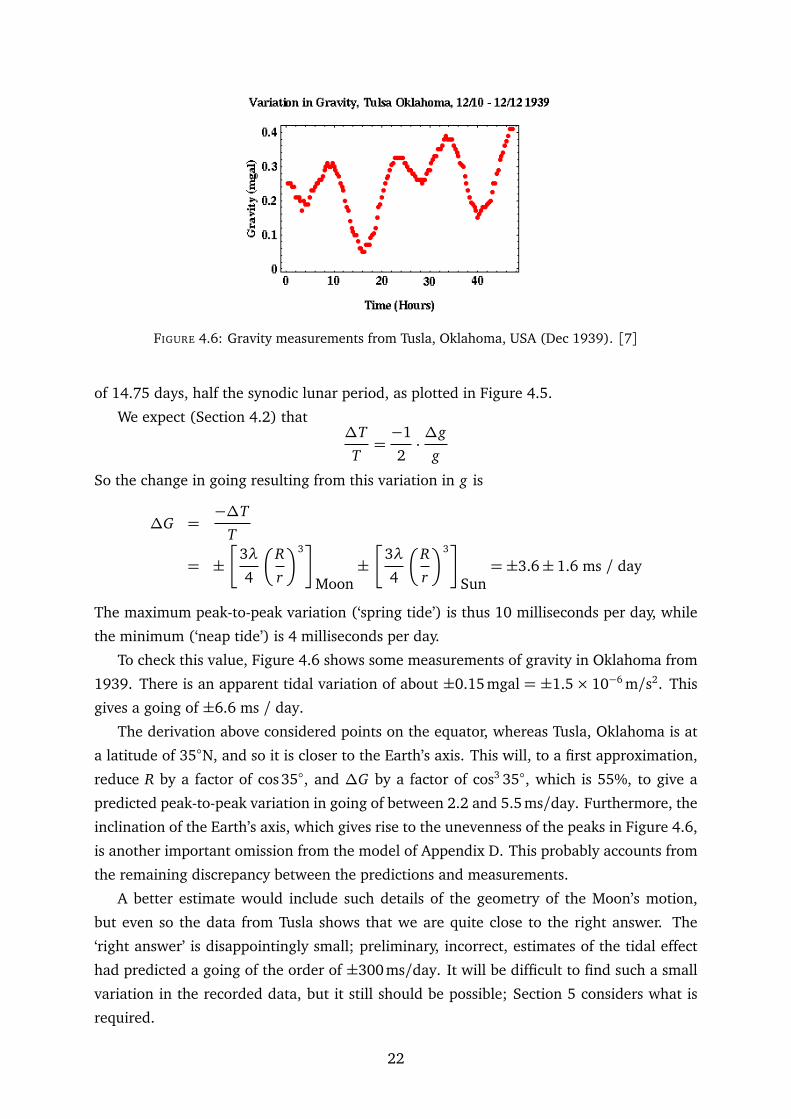
FIGURE 4.6: Gravity measurements from Tusla, Oklahoma, USA (Dec 1939). [7]

of 14.75 days, half the synodic lunar period, as plotted in Figure 4.5.

We expect (Section 4.2) that∆T

T=−1

2·∆g

g

So the change in going resulting from this variation in g is

∆G =−∆T

T

= ±�

3λ

4

�

R

r

�3�

Moon±�

3λ

4

�

R

r

�3�

Sun=±3.6± 1.6 ms / day

The maximum peak-to-peak variation (‘spring tide’) is thus 10 milliseconds per day, while

the minimum (‘neap tide’) is 4 milliseconds per day.

To check this value, Figure 4.6 shows some measurements of gravity in Oklahoma from

1939. There is an apparent tidal variation of about ±0.15 mgal = ±1.5× 10−6 m/s2. This

gives a going of ±6.6 ms / day.

The derivation above considered points on the equator, whereas Tusla, Oklahoma is at

a latitude of 35◦N, and so it is closer to the Earth’s axis. This will, to a first approximation,

reduce R by a factor of cos35◦, and ∆G by a factor of cos3 35◦, which is 55%, to give a

predicted peak-to-peak variation in going of between 2.2 and 5.5ms/day. Furthermore, the

inclination of the Earth’s axis, which gives rise to the unevenness of the peaks in Figure 4.6,

is another important omission from the model of Appendix D. This probably accounts from

the remaining discrepancy between the predictions and measurements.

A better estimate would include such details of the geometry of the Moon’s motion,

but even so the data from Tusla shows that we are quite close to the right answer. The

‘right answer’ is disappointingly small; preliminary, incorrect, estimates of the tidal effect

had predicted a going of the order of ±300ms/day. It will be difficult to find such a small

variation in the recorded data, but it still should be possible; Section 5 considers what is

required.

22

4.6.2 Buoyancy

The buoyancy of the air around the pendulum will decrease its weight (by Archimedes’

Principle), by an amount depending on the air density. The weight of the pendulum is

given by

W = mg −mair g = mg�

1−mair

m

�

= m · g�

1−ρair

ρbob

�

where m is the mass of the pendulum and mair is the mass of air displaced. This effectively

results in a change in gravity of∆g

g=−ρair

ρbob

As before, we expect that∆T

T=−1

2·∆g

g=ρair

2ρbob

so the going resulting from variation in ρair is

G = −∆T

T=−ρair

2ρbob

With a steel pendulum bob of density ρbob = 7800 kg/m3,

dG

dρair=

−1

2ρbob

= −5500 msday−1/kgm−3

4.6.3 Added mass

As the pendulum swings, air will be entrained and move with the pendulum. This effec-

tively increases the pendulum’s inertia without increasing its weight. According to Nelson

and Olsson in [3], this effect results in a change of period of

∆T

T0=

1

2

κmair

m

where κ is a constant representing the fraction of displaced air mair which acts as added

mass. In a perfect, nonviscous fluid in steady-state κ= 1/2, but in reality the value is higher

because the pendulum is accelerating and the fluid has viscosity. A value for κ can be

calculated taking these into account (see [3, §C.3]), and for their example pendulum it is

κ= 1.18. For our purposes we will assume κ∼ 1.

The effect on going is

G =−κ2·ρair

ρbob

∴dG

dρair≈−1

2ρbob

which is about the same as the buoyancy effect.

23

4.6.4 Vertical drag

If there was a vertical flow of air past the pendulum, there would be a drag force acting

on it which would effectively increase or decrease g. No experimental measurements of air

flows around the clock have been made, so this is purely conjecture, but seems possible:

the pendulum extends through the floor of the clock room into a chamber in the wall of the

Fellow’s room below. Since the room below is heated, while the clock room is not, air will

tend to flow up or down through the pendulum chamber.

This force can be estimated using the same drag law used in Section 4.4: F = 12ρV 2SCD.

An upwards force F will cause an effective change in gravity ∆g = −Fm

, where m is the mass

of the pendulum bob. To see if this effect might be important, we can find the air velocity

needed to cause a change in going of, say, −100 ms/day:

∆G =−∆T

T=∆g

2g=−F

2mg

=−ρSCD

4mgV 2

so V =

r

−4mg∆G

ρSCD

Estimating the area and mass of the bob as 0.03 m3 and 100 kg (see Section 4.3), and

assuming CD ≈ 1, this gives V ≈ 0.36m/s. This is actually quite reasonable; it is possible

that this mechanism plays a role but unfortunately without a means of measuring air speed

it is not possible to test it.

Without knowing a typical air velocity, because of the V 2 dependence there is no point

writing this in the form dG/dV , consistent with the other effects.

24

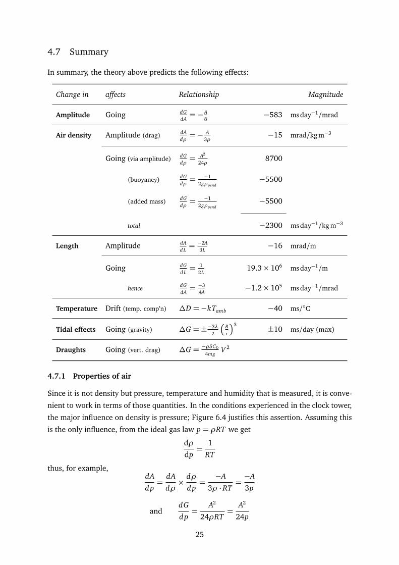
4.7 Summary

In summary, the theory above predicts the following effects:

Change in affects Relationship Magnitude

Amplitude Going dGdA=−A

8−583 ms day−1/mrad

Air density Amplitude (drag) dAdρ=− A

3ρ−15 mrad/kgm−3

Going (via amplitude) dGdρ= A2

24ρ8700

(buoyancy) dGdρ= −1

2gρpend−5500

(added mass) dGdρ= −1

2gρpend−5500

total −2300 ms day−1/kgm−3

Length Amplitude dAd L= −2A

3L−16 mrad/m

Going dGd L= 1

2L19.3× 106 ms day−1/m

hence dGdA= −3

4A−1.2× 105 ms day−1/mrad

Temperature Drift (temp. comp’n) ∆D =−kTamb −40 ms/◦C

Tidal effects Going (gravity) ∆G =±−3λ2

�

Rr

�3±10 ms/day (max)

Draughts Going (vert. drag) ∆G = −ρSCD

4mgV 2

4.7.1 Properties of air

Since it is not density but pressure, temperature and humidity that is measured, it is conve-

nient to work in terms of those quantities. In the conditions experienced in the clock tower,

the major influence on density is pressure; Figure 6.4 justifies this assertion. Assuming this

is the only influence, from the ideal gas law p = ρRT we get

dρ

dp=

1

RT

thus, for example,dA

dp=

dA

dρ×

dρ

dp=

−A

3ρ · RT=−A

3p

anddG

dp=

A2

24ρRT=

A2

24p

25

At a typical pressure of 1010 hPa, this gives dA/dp = −0.018mrad/hPa and dG/dp =0.12 msday−1/hPa.

5 Extracting tidal variations in gravity

We saw in Section 4.6.1 that the tidal variation in gravity will cause a periodic change

in going of at most ±10 milliseconds per day. This is tiny compared to the noise in the

measurements of going, which has an RMS value of about 600 ms/day. Nonetheless spectral

analysis, given a sufficiently long period of data, should be able to discern this periodic

variation from the noise. But how long is ‘sufficiently long’?

The first condition is related to the duration of the data. With a sample rate Fs and data

of duration T , the number of samples is N = FsT . The number of points in the spectrum

is also N , so the bin width ∆ f = Fs/N = 1/T . The tidal variation occurs at a frequency of

approximately 2 cycles per day, the frequency bins must be sufficiently narrow for this to be

distinguishable from lower frequency variations. For example, if we want to find the tidal

variation in the 10th bin, we need ∆ f = 0.2 cycles per day. This means T must be at least

5 days.

The second condition is that the tidal variation be visible above the noise. ‘White’ noise

has a flat spectrum (Figure 5.1), and it is a property of spectra that the area under the

spectrum is equal to the mean square (MS) of the time-domain signal. If the maximum

frequency content of the noise is FN and the amplitude of the spectrum is B2 then

Area under spectrum= 2× 2πFN × B2 =MSnoise

=⇒ B2 =MSnoise

4πFN

The Fourier transform of the periodic tidal variation (with RMS value A) is A2

2δ(ω+ω0) +

A2

2δ(ω−ω0). In a real spectrum, we cannot have infinitely thin δ-functions, so the best

approximation will be that the spike falls into only one frequency bin of width ∆ω and

height C2, say. The areas of the bin and the δ-function must be equal, i.e.

C2∆ω=A2

2

ˆ +∞−∞

δ(ω−ω0)dω=A2

2

−2πFN

A2

2δ(ω+ω0)

B2

2πFN

ω

A2

2δ(ω−ω0)

FIGURE 5.1: Spectrum of Ap

2cosωt and white noise, RMS= B2

26