Introduction to Q-tensor theory

N.J. Mottram∗

Department of Mathematics and Statistics, University of Strathclyde, Livingstone Tower, Glasgow G1 1XH, U.K.

C.J.P. NewtonPeartree Cottage, Little London, Longhope, Gloucestershire GL17 0PH, U.K.

This paper aims to provide an introduction to a basic form of the Q-tensor approach to modellingliquid crystals, which has seen increased interest in recent years. The increase in interest in thistype of modelling approach has been driven by investigations into the fundamental nature of defectsand new applications of liquid crystals such as bistable displays and colloidal systems for which adescription of defects and disorder is essential. The work in this paper is not new research, ratherit is an introductory guide for anyone wishing to model a system using such a theory. A morecomplete mathematical description of this theory, including a description of flow effects, can befound in numerous sources but the books by Virga and Sonnet and Virga are recommended. Moreinformation can be obtained from the plethora of papers using such approaches, although a generalintroduction for the novice is lacking. The first few sections of this paper will detail the developmentof the Q-tensor approach for nematic liquid crystalline systems and construct the free energy andgoverning equations for the mesoscopic dependent variables. A number of device surface treatmentsare considered and theoretical boundary conditions are specified for each instance. Finally, anexample of a real device is demonstrated.

I. BACKGROUND

In all matter, the physical state of the material can be described in terms of the translational and rotationalmotion of the constituent molecules. In a crystalline solid the intermolecular forces hinder motion and force themolecules to lie, on average, in a regular array (i.e. in a crystal lattice structure). As the substance is heatedthe molecules gain kinetic energy and large molecular vibrations break the crystal structure resulting in a fluidphase. In the liquid fluid phase the intermolecular forces are still strong over the average distance betweenmolecules but cannot maintain the crystal structure. In the gas fluid phase the average distance betweenmolecules is large, the intermolecular forces are weak and the unrestricted motion of the molecules cause thegas to expand and fill the container holding it.

In certain materials, which typically consist of either rod-like or disc-like molecules, it is not just the translationalmotion, i.e. the motion of positions of the centres of mass of the molecules, which determines the state of matter.We must also consider the orientation of the rod- or disc-like molecules. In a “normal” liquid, or more correctly,an isotropic liquid, the orientation of the molecule is random. If we pick a single molecule and consider how theorientation varies with time it will eventually take all possible orientations. Alternatively, if we look in a smallregion of the material (say a fixed ball, B, centred at the point x, see Fig. 1(a)), then the molecules in the ballwill be randomly oriented. Such a system, in which a time average is equivalent to a space average, is said tobe ergodic.

However, in a temperature region between the isotropic liquid and crystal states, some materials exhibit anamount of orientational order. That is, if we look in the small ball B the orientation is not random, rather thereexists an average orientation, see Fig. 1(b). Materials which exhibit such orientational order are called liquidcrystals.

A. Measures of orientational order

For such a situation we can define a unit vector n called the director to be the average molecular orientationdirection. For rod-like (or calamitic) molecules this will be the average long axis orientation and for disc-like

∗author for correspondence: nigel.mottram@strath.ac.uk

arX

iv:1

409.

3542

v2 [

cond

-mat

.sof

t] 1

2 Se

p 20

14

2

(a) (b)

B

B+δ

B-δ

FIG. 1: A snap-shot of molecules within the ball B in (a) the isotropic liquid phase and (b) the nematic liquid crystalphase. Due to the head-tail symmetry of the molecules, the order parameter integration need only be performed overthe half sphere δB+ or δB−.

0

f(θ )

θm

m

mθn

0

f(θ )

θm

m

mθn

(a) (b)

FIG. 2: (a) High orientational order: If θm denotes the angle between a molecule and the director and f(θm) is theprobability of finding a molecule with orientation θm in the small region B then for a highly ordered system, f(θm) has asmall standard deviation. (b)Low orientational order: We can still define the average orientation, i.e. the mean of f(θm)but in this case the molecules have more energy and the orientational distribution is more spread out. The standarddeviation of f(θm) is larger.

(discotic) molecules it will be the average orientation of the disc normal. If we consider a different region inthe material the director n may be in a different direction. This director may also vary with time and so it isa variable which is dependent on both space and time coordinates, n(x, t). We can also measure the amountof orientational order about this average direction, in the small ball B. If we consider all the molecules in Band construct a probability distribution of the molecular orientations then the mean of this distribution is thedirector orientation but we can also compute, for instance, the standard deviation of the distribution. Thiswould measure how spread out the molecular orientation distribution is. However, rather than the standarddeviation of this distribution, the usual measure of this amount of order is the scalar order parameter, usuallydenoted by S. This is a weighted average of the molecular orientation angles θm between the long molecularaxes and the director

S =1

2< 3 cos2 θm − 1 >, (1)

where <> denotes the thermal or statistical average so that

S =1

2

∫B

(3 cos2 θm − 1) f(θm) dV, (2)

and f(θm) is the statistical distribution function of the molecular angle θm. Figure 2 shows typical statisticaldistribution functions f(θm) for two cases, high orientational order and low orientational order. The functionf(θm) will be even and periodic due to the head-tail symmetry of the molecules which implies f(θm+π) = f(θm).

In the ball B each molecular orientation can be described by the vector parallel to the molecular long axisor alternatively a point on the surface of a half unit sphere, the point which the molecule “points at” on the

3

x'

y'

z'

θm

φm

FIG. 3: A description of the orientation of a single molecule in terms of the zenithal angle θm and azimuthal angle φm.The x′, y′ and z′ axes are locally defined and are not the laboratory frame of reference.

sphere. The integration in eq. (2) may therefore be performed over half the boundary of the sphere, δB+ sayin Fig. 1(b). An even function of θm must be used in eq. (1) because, since f(θm) is an even function, anyodd function of θm would lead to zero upon integration in eq. (2). To leading order this function is a goodapproximate measure of the orientational order although a more accurate measure would include higher orderpolynomials of cos θm. Equation (1) is in fact the second order Legendre polynomial, P2(cos θm), and it is usualto use the higher order even Legendre polynomials P2n(cos θm) when greater accuracy is required.

When the material is crystalline all molecules align exactly with the director and so θm = 0 for all molecules,which means that < cos2 θm >= 1 and, from eq. (1), S = 1. When all molecules lie in the plane perpendicularto the director, but randomly oriented in that plane, then the average still leads to the same director butθm = π/2 for all molecules so that < cos2 θm >= 0 and S = −1/2. In the isotropic liquid phase the moleculesare randomly oriented and so f(θm) is constant and equal to 1/(2π) (which can be derived from the propertyof probability distributions that

∫f(θm)dV = 1). Therefore, performing the integration in eq. (2) in spherical

coordinates where θm is the angle between the molecule and the director and φm is the azimuthal angle, i.e. theangle between a fixed direction in the plane perpendicular to the director and the projection of the directoronto that plane (see Fig. 3), we obtain (using the substitution x = cos(θm) on the second line),∫

δB+

cos2 θm f(θm) dA =1

2π

∫ 2π

0

∫ π/2

0

cos2 θm sin θmdθm dφm

=

∫ π/2

0

cos2 θm sin θmdθm = −∫ 0

1

x2 dx =1

3(3)

and so < cos2 θm >= 1/3 and from eq. (1), S = 0.

Although it is possible to achieve a molecular configuration for which S is negative, i.e. −1/2 < S < 0, it ismore usual that in the equilibrium liquid crystal state the scalar order parameter is positive, 0 < S < 1. As thetemperature of the material changes the scalar order parameter will change from S = 0 in the isotropic state,at high temperature, to S = 1 in the crystalline state, at low temperature. A typical scalar order parameter inthe middle of the phase region, for this type of liquid crystal, might be S = 0.6.

B. Biaxial nematics

The fundamental principle of any biaxial system is that there is no axis of complete rotational symmetry (i.eno axis about which a rotation of any angle leaves the system unchanged), unlike a uniaxial system which hasan axes of rotational symmetry (such as the director n in uniaxial liquid crystals). For instance, some solidmaterials (i.e. calcite) are uniaxial, and therefore birefringent, so that light travelling along the optical axis seesa different refractve index than light travelling perpendicular to the optic axis. However, other materials arebiaxial (i.e. olivine), and have trirefringence, where there are three different refractive indices, for light travellingalong three orthogonal directions.

For such biaxial materials there can be defined a set of perpendicular axes (only two need to be defined asthe third is then specified as perpendicular to the other two) for each of which there is a reflection symmetry.

4

In biaxial liquid crystals the two axes n and m are therefore defined and the symmetries are the reflectionsn→ −n and m→ −m.

The definition of three axes of reflective symmetry in a material is a relatively straightforward concept. Lessstraightforward is to understand the molecular arrangement corresponding to a biaxial systems. There are twopossibilities for the shape of the molecules: either the molecules are uniaxial or they are biaxial. A uniaxialmolecule can be thought of as shaped like a cylinder or rod (uniaxial because there is a rotation symmetryabout the axis of the molecule), a biaxial molecule might be shaped like a plank of wood. There is no rotationaxis along the long axis of the plank (rotating the plank changes its configuration) but there are three axes ofreflective symmetry (the long, intermediate and short axis of the plank).

We can now have a uniaxial or biaxial arrangement of uniaxial molecules and a uniaxial or biaxial arrangementof biaxial molecules. The easiest arrangements to imagine are the uniaxial arrangement of uniaxial molecules - agroup of cylindrical molecules oriented, on average, along a single direction where rotation about this directiondoes not alter, at least statistically speaking, the arrangement - and also the biaxial arrangement of biaxialmolecules, a group of plank-shaped molecules where the long axes of the planks align in one direction and theshort axes also align, in a second direction, so creating a biaxial ensemble arrangement.

A uniaxial arrangement of biaxial molecules is also relatively easy to imagine. In this arrangement the molecularlong axes orient as before but the short axes of the plank are oriented randomly so that, if we view from theside as in Fig. 1, at any moment in time some of the planks are facing out of the page and some are turned endon. When you rotate the system the individual molecules look different but on average the same proportion ofmolecules are face on and end on (and all orientations in between).

A more difficult situation to imagine is a biaxial arrangement of uniaxial molecules. Such an alignment isdescribed below and is the most relevant to the liquid crystal structure at the centre of defects.

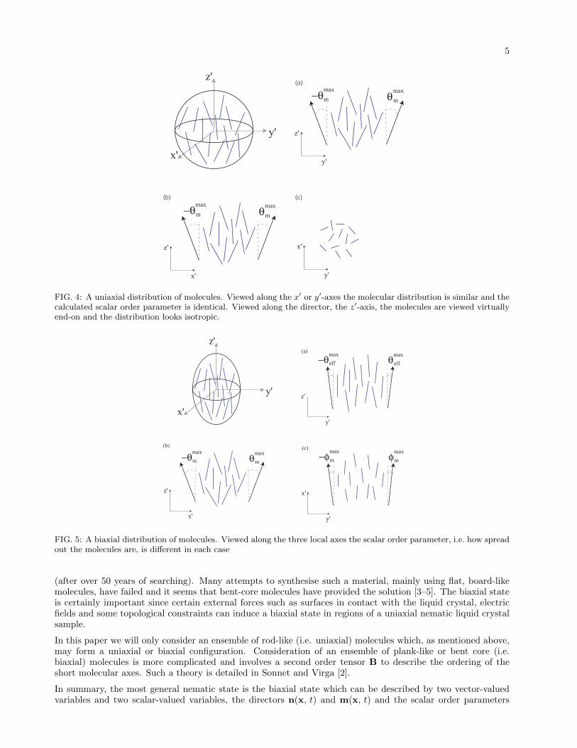
Imagine a group of uniaxial molecules (the cylindrical or rod-like molecules) which are in a uniaxial arrangement(Fig. 4) if you look down the director (the z′ axis) the molecules, which are now viewed almost end-on, lookrandom, it is only the side view (along the x′ or y′ axis) which indicates the director n. Now restrict this groupof molecules by “squashing” the distribution within the ball (see Fig. 5) between two imaginary plane surfacesparallel to the x′z′ plane, and look along the z′ axis again. There will be a restriction of the motion of themolecules in Fig. 4(c) to an arrangement similar to Fig. 5(c).

In more mathematical terminology: in the ball B, if the distribution of molecules is such that the zenithal anglesθm vary between −θmaxm and θmaxm and the azimuthal angles vary between −φmaxm and φmaxm then the three viewsof the group of molecules along the x′, y′ and z′ axes are shown in Fig. 5(a), (b) and (c) respectively. If welook at the molecules along the y′-axis (Fig. 5(b)) the extent of the zenithal angle is −θmaxm < θm < θmaxm andwe can define a scalar order parameter S1. If we look at the molecules along the z′-axis (Fig. 5(c)) the extentof the azimuthal angle is −φmaxm < φm < φmaxm and we can define a scalar order parameter S2 say. If we lookalong the x′-axis (Fig. 5(a)), the restriction to the azimuthal angle means we see an effective zenithal anglerange which is smaller than in Fig. 5(a). Simple geometry gives us that the effective range of zenithal angles isnow

− θmaxeff = − tan−1 (sinφmaxm tan θmaxm ) < θm < tan−1 (sinφmaxm tan θmaxm ) = θmaxeff (4)

Therefore, with this view, we would calculate a different scalar order parameter, S3 say which is larger than S1

(in fact S3 is related to S1 and S2). It is now necessary to define three directors and corresponding scalar orderparameters. If we take two perpendicular directors n and m, in our situation the z′ and y′ directions, then wecan define the two scalar order parameters S1 and S2 associated with order about the two directors respectively(the third director being n ×m). If the order parameter S2 is non-zero and not equal to S1 the liquid crystalis said to be biaxial, i.e. there are two axes of symmetry. If, however, S2=0 then in comparison to Fig. 5(c)the range of azimuthal angles is now −π/2 < φm < π/2 and a view along the z′-axis shows randomly orientedmolecules (see Fig. 4). The view from the x′-axis will show a regular nematic distribution of molecules and thedirector and a non-zero order parameter S1 can be defined. Since the system of molecules is now rotationallysymmetric about the z′-axis, the view along the y′ axis will be the same as that along the x′-axis and thus theorder parameter will again be S1.

From these examples we see that the uniaxial nematic state exists when the order parameter with respect toone direction is zero, or equivalently the order parameters with respect to the perpendicular directions are thesame. The biaxial nematic state exists when the scalar order parameters in all three perpendicular directionsare different.

It should be mentioned that a stable biaxial thermotropic nematic liquid crystal has only recently been reported

5

m−θmax

mθmax

(b)

x'

z'

(a)

y'

z'

(c)

y'

x'

m−θmax

mθmax

x'

y'

z'

FIG. 4: A uniaxial distribution of molecules. Viewed along the x′ or y′-axes the molecular distribution is similar and thecalculated scalar order parameter is identical. Viewed along the director, the z′-axis, the molecules are viewed virtuallyend-on and the distribution looks isotropic.

m−θmax

mθmax

(b)

x'

z'

eff−θmax

effθmax

(a)

y'

z'

m−φmax

mφmax

(c)

y'

x'

x'

y'

z'

FIG. 5: A biaxial distribution of molecules. Viewed along the three local axes the scalar order parameter, i.e. how spreadout the molecules are, is different in each case

(after over 50 years of searching). Many attempts to synthesise such a material, mainly using flat, board-likemolecules, have failed and it seems that bent-core molecules have provided the solution [3–5]. The biaxial stateis certainly important since certain external forces such as surfaces in contact with the liquid crystal, electricfields and some topological constraints can induce a biaxial state in regions of a uniaxial nematic liquid crystalsample.

In this paper we will only consider an ensemble of rod-like (i.e. uniaxial) molecules which, as mentioned above,may form a uniaxial or biaxial configuration. Consideration of an ensemble of plank-like or bent core (i.e.biaxial) molecules is more complicated and involves a second order tensor B to describe the ordering of theshort molecular axes. Such a theory is detailed in Sonnet and Virga [2].

In summary, the most general nematic state is the biaxial state which can be described by two vector-valuedvariables and two scalar-valued variables, the directors n(x, t) and m(x, t) and the scalar order parameters

6

x

y

z

θ

φ

nm

ψ

FIG. 6: The directors n and m in terms of the Euler angles θ, φ and ψ. The axes x, y and z form the laboratory frameof reference.

S1(x, t) and S2(x, t), all of which may depend on the spatial coordinates x and time.

We assume, without loss of generality, that the directors are of unit length, |n| = 1 and |m| = 1. Just as wehave described each molecule in Fig. 3, each of these directors can be represented in terms of the standard Eulerangles, see Fig. 6. Since the director n is of unit length it can be written as,

n = (cos θ cosφ, cos θ sinφ, sin θ) . (5)

It is important not to confuse the director angles θ and φ with the molecular angles in Fig. 3. The molecularangles θm and φm are angles relative to a local frame of reference, i.e. the directors, whereas the angles θ andφ are defined relative to the laboratory frame of reference, i.e a set of axes fixed in space, independent of theorientation of the material.

The director m is perpendicular to n and therefore has one remaining degree of freedom, the angle ψ,

m = (sinφ cosψ − cosφ sinψ sin θ, − sinφ sinψ sin θ − cosφ cosψ, sinψ cos θ) . (6)

The angle ψ is the angle from m to the direction (sinφ, − cosφ, 0) in the xy-plane which is also perpendicularto n.

A theory can now be constructed using the five dependent variables,

θ(x, t), φ(x, t), ψ(x, t), S1(x, t), S2(x, t). (7)

However, there may be problems with a theory such as this, based on Euler angles. When the zenithal angleθ equals π/2 the azimuthal angle φ is undefined and, as with all such angle variables, there may also be aproblem with multi-valuedness since φ = 0 is equivalent to φ = 2π. Care must be taken when solving governingdifferential equations for θ, φ and ψ.

C. The tensor order parameter Q

We now define an alternative approach which removes the problems of the angle representation described above.Instead of defining the nematic state in terms of the five separate variables in eq. (7) we construct a 3x3 matrixwhich contains all the information about the nematic state, i.e. the information contained in the five variables.The problems of solving the Euler angle governing equations will be removed with this approach (for referencesee for example [1, 2]).

Consider the 3x3 matrix,

M = S1 (n⊗ n) + S2 (m⊗m) , (8)

where, for any vector h the ijth element of the product h ⊗ h is hi hj , the ith element of h multiplied by thejth element of h. This matrix will be symmetric, since ni nj = nj ni and mimj = mjmi, and the trace of Mwill be S1(n1n1 + n2n2 + n3n3) + S2(m1m1 +m2m2 +m3m3) = S1 + S2 since |n| = 1 and |m| = 1

Since the trace of M is fixed and the matrix is symmetric, M will have five independent elements,

M =

m1 m2 m3

m2 m4 m5

m3 m5 (S1 + S2)−m1 −m4

(9)

7

The tensor M contains the same information as the five separate variables in eq. (7). However, if we constructa theory using M there will be no problems with the degeneracies of Euler angles.

As will be indicated later, it is actually more useful to use the tensor,

Q = S1 (n⊗ n) + S2 (m⊗m)− 1

3(S1 + S2)I, (10)

where I is the identity matrix so that the trace of Q is zero. The tensor order parameter Q is therefore asymmetric traceless matrix and can be written as,

Q =

q1 q2 q3q2 q4 q5q3 q5 −q1 − q4

, (11)

and from the definitions of n and m and eqs (10) and (11) we see that the elements qi can be written in termsof the variables θ, φ, ψ, S1 and S2 thus,

q1 = S1 cos2 θ cos2 φ+ S2 (sinφ cosψ − cosφ sinψ sin θ)2 − 1

3(S1 + S2), (12)

q2 = S1 cos2 θ sinφ cosφ

−S2 (cosφ cosψ + sinφ sinψ sin θ) (sinφ cosψ − cosφ sinψ sin θ) , (13)

q3 = S1 sin θ cos θ cosφ+ S2 sinψ cos θ (sinφ cosψ − cosφ sinψ sin θ) , (14)

q4 = S1 cos2 θ sin2 φ+ S2 (cosφ cosψ + sinφ sinψ sin θ)2 − 1

3(S1 + S2), (15)

q5 = S1 cos θ sin θ sinφ− S2 sinψ cos θ (cosφ cosψ + sinφ sinψ sin θ) . (16)

From the previous section, the description of biaxiality tells us that, if the matrix Q was diagonalised (so thatthe eigenvectors are along the x′, y′ and z′ directions) then for a uniaxial state two of the eigenvalues would bethe same and for a biaxial state all three eigenvalues would be different.

The eigenvalues of the matrix Q, described by eqs (12)-(16), are,

λ1 = (2S1 − S2)/3, (17)

λ2 = −(S1 + S2)/3, (18)

λ3 = (2S2 − S1)/3. (19)

Uniaxial states exist when two of these eigenvalues are the same i.e. when λ1 = λ2 so that S1 = 0 or whenλ2 = λ3 so S2 = 0 or when λ1 = λ3 so S1 = S2. When all the eigenvalues are the same we have an isotropicsystem and we have S1 = 0 and S2 = 0 so that Q = 0. We shall see later that the use of Q rather than Mas our dependent tensor variable was in fact dictated by the property that the isotropic state is described byQ = 0.

If we, for simplicity, define our laboratory axes to be such that the directors n and m are in the directions ofthe x and y axes then θ = 0, φ = 0 and ψ = π so that

q1 =1

3(2S1 − S2), (20)

q2 = 0, (21)

q3 = 0, (22)

q4 =1

3(2S2 − S1), (23)

q5 = 0, (24)

and therefore the three possible uniaxial states correspond to: q1 = −q1 − q4 so that q1 = −q4/2 = −S2/3;−q1 − q4 = q4 so that q4 = −q1/2 = −S1/3; or q1 = q4 = S1/3 = S2/3.

There will be no problems when solving the governing equations for the five dependent variables q1, q2, q3, q4, q5because the Euler angles only appear in sin and cos functions and the problem with the multivaluedness of theangles is removed.

8

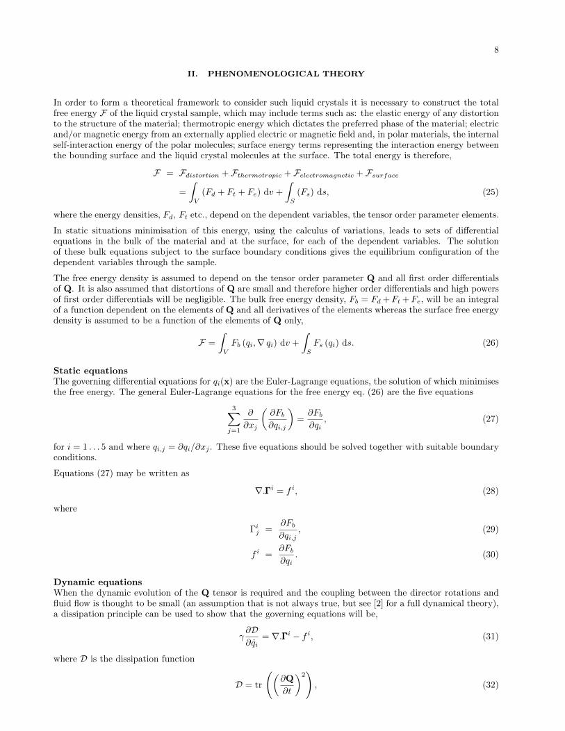
II. PHENOMENOLOGICAL THEORY

In order to form a theoretical framework to consider such liquid crystals it is necessary to construct the totalfree energy F of the liquid crystal sample, which may include terms such as: the elastic energy of any distortionto the structure of the material; thermotropic energy which dictates the preferred phase of the material; electricand/or magnetic energy from an externally applied electric or magnetic field and, in polar materials, the internalself-interaction energy of the polar molecules; surface energy terms representing the interaction energy betweenthe bounding surface and the liquid crystal molecules at the surface. The total energy is therefore,

F = Fdistortion + Fthermotropic + Felectromagnetic + Fsurface

=

∫V

(Fd + Ft + Fe) dv +

∫S

(Fs) ds, (25)

where the energy densities, Fd, Ft etc., depend on the dependent variables, the tensor order parameter elements.

In static situations minimisation of this energy, using the calculus of variations, leads to sets of differentialequations in the bulk of the material and at the surface, for each of the dependent variables. The solutionof these bulk equations subject to the surface boundary conditions gives the equilibrium configuration of thedependent variables through the sample.

The free energy density is assumed to depend on the tensor order parameter Q and all first order differentialsof Q. It is also assumed that distortions of Q are small and therefore higher order differentials and high powersof first order differentials will be negligible. The bulk free energy density, Fb = Fd +Ft +Fe, will be an integralof a function dependent on the elements of Q and all derivatives of the elements whereas the surface free energydensity is assumed to be a function of the elements of Q only,

F =

∫V

Fb (qi,∇ qi) dv +

∫S

Fs (qi) ds. (26)

Static equationsThe governing differential equations for qi(x) are the Euler-Lagrange equations, the solution of which minimisesthe free energy. The general Euler-Lagrange equations for the free energy eq. (26) are the five equations

3∑j=1

∂

∂xj

(∂Fb∂qi,j

)=∂Fb∂qi

, (27)

for i = 1 . . . 5 and where qi,j = ∂qi/∂xj . These five equations should be solved together with suitable boundaryconditions.

Equations (27) may be written as

∇.ΓΓΓi = f i, (28)

where

Γij =∂Fb∂qi,j

, (29)

f i =∂Fb∂qi

. (30)

Dynamic equationsWhen the dynamic evolution of the Q tensor is required and the coupling between the director rotations andfluid flow is thought to be small (an assumption that is not always true, but see [2] for a full dynamical theory),a dissipation principle can be used to show that the governing equations will be,

γ∂D∂qi

= ∇.ΓΓΓi − f i, (31)

where D is the dissipation function

D = tr

((∂Q

∂t

)2), (32)

9

qi = ∂q/∂xi and the viscosity γ is related to the standard nematic viscosity γ1 (which is equal to α3 − α2 inLeslie viscosities) by,

γ =γ1Sexp

, (33)

where Sexp is the uniaxial order parameter of the liquid crystal when the experimental measurement of γ1 wastaken.

Boundary conditionsTwo types of boundary conditions will be considered; strong (infinite) or weak anchoring.

(i) Strong: For strong, also termed infinite, anchoring we use Dirichlet conditions. That is, the order tensorwill be fixed at a specified value at the domain boundary that has been dictated by some substrate alignmenttechnique. In this case the boundary condition is

Q = Qs, (34)

where Qs is the prescribed order tensor at the boundary. In this case there is no surface energy and Fs = 0 ineq. 25.

(ii) Weak: For a weak anchoring effect there exists a surface energy, Fs, which is added to the free energy andmust be minimised at the same time as the bulk free energy. This minimisation leads to the condition that, onthe boundary, the liquid crystal variables qi satisfy∑

j=1,2,3

νj

(∂Fb∂qi,j

)=∂Fs∂qi

(35)

or equivalently

ννν.ΓΓΓi = Gi (36)

where ΓΓΓi is as in eq. (29), Gi = −∂Fs/∂qi and where ννν is the normal to the substrate. Usually the surface isplanar or circular so that the surface normal is relatively simple, for example ννν = (0, 0, 1) if the surface is aplane parallel to the xy-plane. However, in general the substrate normal is position dependent ννν(x).

In order to complete this theory it is necessary to specify each of the components of the free energy. Thefollowing sections describe the thermotropic, elastic, electrostatic and surface energies.

A. Landau-de Gennes thermotropic energy

The thermotropic energy, Ft, is a potential function which dictates which state the liquid crystal would preferto be in, i.e. a uniaxial state, a biaxial state or the isotropic state. At high temperature this potential shouldhave a minimum energy in the isotropic state, i.e. Q = 0 whereas at low temperatures there should be minimaat three uniaxial states, i.e. the states where any two of the eigenvalues of Q are equal. For rod-like moleculesa bulk biaxial minimum energy state is not possible[2]. The simplest form of such a function is a truncatedTaylor expansion about Q = 0 [6],

Ft = a tr(Q2)

+2b

3tr(Q3)

+c

2

(tr(Q2))2

(37)

which is a quartic function of the qis. This energy is sometimes written as

Ft = a tr(Q2)

+2b

3tr(Q3)

+ c tr(Q4). (38)

Equations (37) and (38) are equivalent only if the factor of two in the c term is included. This form of energycan also be thought of as an expansion in terms of the two invariants of the order tensor, tr

(Q2)

and det(Q).

The coefficients a, b and c will in general be temperature dependent although it is usual to approximate thisdependency by assuming that b and c are independent of temperature whilst a = α(T − T ∗) = α∆T whereα > 0 and T ∗ is the fixed temperature at which the isotropic state becomes unstable.

10

As stated in Section I C, the eigenvalues of Q are λ1 = (2S1−S2)/3, λ2 = −(S1 +S2)/3, λ3 = (2S2−S1)/3 andsince the trace of the nth power of Q is the sum of the nth powers of these eigenvalues, thus the thermotropicenergy is simply a function of S1 and S2,

Ft = a

3∑i=1

λ2i +2b

3

3∑i=1

λ3i +c

2

(3∑i=1

λ2i

)2

(39)

=2a

3

(S21 − S1S2 + S2

2

)+

2b

27

(2S3

1 − 3S21S2 − 3S1S

22 + 2S3

2

)(40)

+2c

9

(S41 − 2S3

1S2 + 3S21S

22 − 2S1S

32 + S4

2

)For a uniaxial state such as λ2 = λ3, or equivalently S2 = 0, the thermotropic energy becomes,

Ft =2

27

(9aS2

1 + 2bS31 + 3cS4

1

)(41)

Which has stationary points when dFt/dS1 = 0 so that,

S1 = 0 (42)

S1 =1

4c

(−b+

√b2 − 24ac

)(43)

S1 =1

4c

(−b−

√b2 − 24ac

)(44)

This calculation can be performed using the qi variables if we first assume for simplicity that the laboratoryframe of reference is set such that the directors are along the axes, as in Section I B. In this case we obtain thestationary points of the free energy as,

q1 = 0 (45)

q1 =1

6c

(−b+

√b2 − 24ac

)(46)

q1 =1

6c

(−b−

√b2 − 24ac

)(47)

By calculating d2Ft/dS21 and comparing the energies of each solution we find that

• S1 = 0, the isotropic state, is globally stable for a > b2

27c , metastable for 0 < a < b2

27c and unstable fora < 0.

• S1 = 14c

(−b+

√b2 − 24ac

), the nematic state, is globally stable for a < b2

27c , metastable for b2

27c < a < b2

24c

and not defined for a > b2

24c .

• S1 = 14c

(−b−

√b2 − 24ac

)is metastable (but has a negative value) for a < 0, unstable for b2

27c < a < b2

24c

and not defined for a > b2

24c .

The equilibrium nematic scalar order parameter (43) will be denoted by Seq.

There are clearly three important values of a: a = b2

24c , the high temperature where the nematic state disappears;

a = b2

27c , the temperature at which the energy of the isotropic and nematic states are exactly equal; a = 0, thelow temperature where the isotropic state loses stability. If we use the notation a = α(T −T ∗) then the critical

temperatures are T+ = b2

24αc + T ∗; TNI = b2

27αc + T ∗; T = T ∗.

Therefore, for this thermotropic energy and depending on the values of the coefficients a, b and c, in anintermediate temperature region the minimum at the isotropic state and the minima at the uniaxial nematicstates may all be locally stable. However, at sufficiently low temperatures the isotropic state must lose stabilityleaving only the uniaxial nematic states stable and at sufficiently high temperatures the uniaxial states mustlose stability leaving only the isotropic state stable. The thermotropic potential function is shown in Figs 7 and

11

–0.4

–0.2

0

0.2

0.4

0.6

q1

–0.4

–0.2

0

0.2

0.4

0.6

q4

0

2000

4000

6000

8000

10000

–0.4

–0.2

0

0.2

0.4

0.6

q1

–0.4

–0.2

0

0.2

0.4

0.6

q4

0

2000

4000

6000

8000

10000

–0.4

–0.2

0

0.2

0.4

0.6

q1

–0.4

–0.2

0

0.2

0.4

0.6

q4

0

2000

4000

6000

8000

10000

–0.6–0.4

–0.20

0.20.4

0.60.8

q1

–0.6–0.4

–0.200.2

0.40.6

0.8

q4

–8000

–6000

–4000

–2000

0

2000

4000

6000

8000

10000

–0.6–0.4

–0.20

0.20.4

0.60.8

q1

–0.6–0.4

–0.200.2

0.40.6

0.8

q4

–20000

–15000

–10000

–5000

0

5000

10000

–0.6–0.4

–0.20

0.20.4

0.60.8

q1

–0.6–0.4

–0.200.2

0.40.6

0.8

q4

–20000

–15000

–10000

–5000

0

5000

10000

Ft

(a) (b)

(c)

(e) (f)

(d)

FIG. 7: The thermotropic potential for parameters α = 0.042×106Nm−2K−1, b = −0.64×106Nm−2, c = 0.35×106Nm−2

[7] and (a) ∆T = 2.0, (b) ∆T = 1.5, (c) ∆T = 1.0, (d) ∆T = 0.5, (e) ∆T = 0.0, (f) ∆T = −0.1. At high temperatures(a,b) only the isotropic state is stable and at low temperature (d,e,f) the three uniaxial states are stable. At intermediatetemperatures (c) both the isotropic and all three nematic states are stable.

8. In these figures the tensor order parameter is assumed to be diagonalised so that the directors align with thelaboratory frame of reference. Therefore, as mentioned in Section I C, the off diagonal terms of Q are zero andFt depends only on q1 and q4. Figure 7(a) clearly shows the three uniaxial states and as temperature increasesthe potential function changes to exhibit a single minima at the isotropic state.

This expression for the thermotropic energy, eq. (37), is essentially a Taylor series of the true thermotropicenergy, close to the point Q = 0. Therefore we must remember that the Landau-de Gennes theory is only validclose to the nematic-isotropic transition temperature, TNI , where Q ≈ 0. It is for this reason that we may

12

–20000

–10000

0

10000

20000

30000

–0.2 0 0.2 0.4 0.6 0.8

q1

Ft

ΔT=0.5

ΔT=0.0

ΔT=0.5

ΔT=-0.1

ΔT=1.0

ΔT=2.0

FIG. 8: Cross-section of Fig. 7 along the line q4 = q1/2, the equivalent to the uniaxial state S2 = 0, for varyingtemperature with the parameter values α = 0.042× 106Nm−2K−1, b = −0.64 × 106Nm−2, c = 0.35 × 106Nm−2 [7]. At∆T = 0.5 both the isotropic minima (q1 = 0) and the uniaxial nematic minima (q1 6= 0) are locally stable.

assume that higher order powers of Q may be neglected in eq. (37). The first five powers of Q are includedin eq. (37) (the constant term is neglected as it will not enter into a minimisation of the energy and the linearterm is taken to have zero coefficient since tr(Q) = 0 so that there is a minimum at Q = 0) since we assumethere are at most four minima in the potential function Ft.

It would be energetically favourable for the system to lie in one of the minima of Ft. When a liquid crystalmaterial is forced to contain some form of distortion (e.g. through the influence of surface or electric fieldeffects) there are two mechanisms for undertaking such a distortion. For example imagine a region of liquidcrystal constrained to lie between two solid surfaces. If, through some surface treatment, one of the surfacesforces the liquid crystal in contact with that surface to lie in a fixed uniaxial state, i.e in one of the minima ofFig. 7(a) whereas the other surface forces the liquid crystal in contact with it to lie in a different uniaxial state.Firstly, for the system to move from one minima of Ft to another, the eigenvectors of Q may change. This isequivalent to the molecular frame of reference changing. The system effectively rotates the picture in Fig. 7so that the system always remains in the same minima of Ft, it is simply that the minima itself that changesposition. Alternatively, the eigenvalues of Q may change but the eigenvectors remain fixed. This is equivalentto the picture in Fig. 7 remaining fixed and the system distorting from one uniaxial state to another through abiaxial state, see Fig. 9. Such a transformation is often termed eigenvalue exchange. Alternatively, there maybe a combination of eigenvector and eigenvalue distortions and exactly how the system distorts will depend onthe competition between the thermotropic energy Ft and the elastic energy Fd.

13

–1

–0.5

0

0.5

1

q

–1

–0.5

0

0.5

1

1

4q

tF

FIG. 9: A schematic plot of how a system may be forced out of the thermotropic potential minimum. At one point inthe liquid crystal (represented by one end point of the yellow line) the system is forced, through some external agent, tolie at one of the uniaxial states. At another point in the liquid crystal (represented by the other end point of the yellowline) the system is forced to lie in a different uniaxial states. For the macroscopic variables to be continuous throughthe region the system continuously transforms from one state to the other, at some points moving out of the potentialminima. The yellow line plots the state variables on the potential energy surface of the system from one region in theliquid crystal to the other.

B. Elastic energy

The distortional or elastic energy density, Fd, of a liquid crystal is derived from the energy induced by distortingthe Q tensor in space. It is, generally, energetically favourable for Q to be constant throughout the materialand any gradients in Q would lead to an increase in distortional energy. Fd therefore depends on the spatialderivatives of Q. Given a fixed distortion in space of Q the distortional energy must remain unchanged if wewere to translate or rotate the material. Such restrictions (or symmetries) mean that not all combinations ofQ derivatives are allowed. In fact the elastic energy may be simplified to [8],

Fd =∑

i=1,2,3j=1,2,3k=1,2,3

[L1

2

(∂Qij∂xk

)2

+L2

2

∂Qij∂xj

∂Qik∂xk

+L3

2

∂Qik∂xj

∂Qij∂xk

]

+∑

i=1,2,3j=1,2,3k=1,2,3l=1,2,3

[L4

2elikQlj

∂Qij∂xk

+L6

2Qlk

∂Qij∂xl

∂Qij∂xk

]. (48)

The coordinates (x1, x2, x3) = (x, y, z) are the usual Cartesian coordinate system and Qij is the ijth elementof Q. The first four terms are quadratic in the scalar order parameters S1 and S2 whereas the last term is cubicin the scalar order parameters.

14

The elastic parameters Li are related to the Frank elastic constants kij by [8]

L1 =1

6S2exp

(k33 − k11 + 3k22), (49)

L2 =1

S2exp

(k11 − k22 − k24), (50)

L3 =1

S2exp

k24, (51)

L4 =2

S2exp

q0k22, (52)

L6 =1

2S3exp

(k33 − k11), (53)

where Sexp is the uniaxial order parameter of the liquid crystal when the experimental measurement of the

Li was taken and may not be equal to the current order parameter Seq =(−b+

√b2 − 24ac

)/(4c) mentioned

in Section II A. The parameter q0 is the chirality of the liquid crystal and if an achiral liquid crystal is underconsideration then L4 = 0.

It has been shown that there are seven elastic terms of cubic order [9, 10] but we will only include one, the L6

term in eq. (48), in order to ensure we can model a nematic state with non-equal elastic constants k11, k22, k33.Without the L6 term we have four elastic parameters L1, . . . , L4 in the Q tensor elastic energy but we have fiveindependent parameters in the Frank approach, k11, k22, k33, k24 and q0. Including the L6 term removes thedegeneracy in the mapping from the Q tensor to the Frank energy approaches.

C. Electrostatic energy

The liquid crystal will interact with an externally applied electric field or indeed self-induce an internal electricfield due to the dielectric and spontaneous polarisation effects. The electrostatic energy density is

Fe = −∫

D.dE, (54)

where D is the displacement field and E is the electric field. The constitutive equation,

D = ε0E + P

= ε0E + Pi + Ps

= ε0E + ε0χχχE + Ps

= ε0εεεE + Ps, (55)

relates the displacement field with the electric field E and the internal polarisation P. This polarisation is splitinto dielectrically induced polarisation Pi and the spontaneous polarisation Ps. The induced polarisation isdependent on the dielectric susceptibility χ and the electric field E and the dielectric tensor is then defined asε = I + χ where I is the identity matrix. The electrostatic energy density is then,

Fe = −∫

(ε0εεεE + Ps).dE = −1

2ε0 (εεεE) .E−Ps.E. (56)

In a nematic liquid crystal the dielectric tensor is approximated to εεε = ∆ε∗Q + εI where ∆ε∗ = (ε|| − ε⊥)/Sexpis the scaled dielectric anisotropy and ε = (ε||+ 2ε⊥)/3 is an average permittivity. Within an isotropic material,such as an alignment layer of photo-resist material, the dielectric tensor is diagonal and isotropic, ε = εII.

In the present, nematic, situation a spontaneous polarisation vector is assumed to derive only from a flexoelectrictype of polarisation, that is a polarisation caused by a distortion of the molecular arrangement. This may bedue to a shape asymmetry in the molecules or due to a distortion of a pair-wise coupling of molecules. Foreither of these mechanisms, the polarisation may be written, to leading order, in terms of the Q tensor as [11],

Ps = e∇.Q, (57)

15

where the ith component of ∇.Q is understood to be∑j=1,2,3 ∂Qij/∂xj .

If we consider the flexoelectric polarisation of a uniaxial state, where Q = S ((n⊗ n)− I/3), we find

Ps = e

(S (∇.n) n + S (∇× n)× n + (n.∇S) n− 1

3∇S). (58)

Comparing this to the standard expressions for flexoelectric polarisation and order electricity [12–14],

Pf = e11 (∇.n) n + e33 (∇× n)× n, (59)

Po = r1 (n.∇S) n + r2∇S, (60)

we see that eq. (57) is equivalent to eqs (59) and (60) when we set e11 = e33 = Se and r1 = e, r2 =−e/3. Therefore, without taking higher order terms in eq. (57), this expression assumes that the coefficientsof flexoelectric and order electric terms are equal. Within a region where S is constant, only the flexoelectricpolarisation eq. (59) would be present.

In order to distinguish between the flexoelectric parameters e11 and e33 higher order terms are needed in theflexoelectric polarisation term in eq. (57) [15]. For instance, if we include second order terms the ith componentof the polarisation vector is

(Ps)i = p1∑

j=1,2,3

∂Qij∂xj

+ p2∑

j=1,2,3k=1,2,3

Qij∂Qjk∂xk

+ p3∂

∂xi

∑j=1,2,3k=1,2,3

QjkQjk

+ p4∑

j=1,2,3k=1,2,3

Qjk∂Qji∂xk

. (61)

For a uniaxial material we can substitute, expand and collect terms as before. This gives

e11 = Sp1 +S2

3(2p2 − p4),

e33 = Sp1 +S2

3(2p4 − p2),

r1 = p1 +S

3(p2 + p4),

r2 =1

3

(−p1 +

S

3(p2 + p4) + 4Sp3

).

Therefore, including second order terms does allow us to have different values for e11 and e33 if p2 6= p4. However,deciding on values for p1 . . . p4 is non-trivial. Barbero et al. [14] have stated that p1, p2 and p4 can be obtainedby measuring the flexoelectric parameters as a function of temperature, and assume a similar magnitude for p3,but there seems to be no such measurements in the literature.

At this point the electric field within the whole cell is unknown but may be found using Maxwell’s equationswhich are, in this static case with no free charges,

∇.D = 0, (62)

∇×E = 0. (63)

Equation (63) means that we may define a scalar function U , the electric potential, which satisfies E = −∇U(it is convention to make E the negative gradient of U). If we find the function U then eq. (63) is automaticallysatisfied. Equation (62) is then the governing equation for the electric potential U ,

0 = ∇.D = ∇. (−ε0εεε∇U + Ps) , (64)

and the free energy density,

Fe = −1

2ε0εεε∇U.∇U + Ps.∇U, (65)

will enter the total free energy density to be minimised in order to obtain the Euler-Lagrange equations for theqi. Equation (64) is in fact equivalent to the Euler-Lagrange equation derived from minimising the free energyin eq. (65) with respect to U .

At any material boundary (i.e. between the liquid crystal and a substrate) we must ensure that the standardconditions of electrostatics are obeyed, that the electric potential U continuous, the component of the displace-ment field normal to the boundary is continuous and the component of the electric field parallel to the boundaryis continuous. The external boundary conditions for U are usually set at the electrodes where, for example, oneelectrode is set to be earthed and so U = 0 and the other electrode is set to be a fixed voltage U = V .

16

D. Surface energy

When the liquid crystal molecules are close to a solid surface they will feel a molecular interaction force.Whatever this force is we would like to model this liquid crystal-surface interaction in a macroscopic framework.That is, how does the surface interact with the macroscopic variables (the elements of the tensor order parameterQ). If the surface is treated is some way, usually by coating the surface with a chemical and possibly rubbingthe surface in a fixed direction so as to create a preferred surface direction, then we will assume that at thatsurface the directors n and m would prefer to lie in a certain direction. We may also assume that the solidsurface may affect the amount of order (i.e. the variables S1 and S2) at that surface. Associated with thispreference for a certain orientation and order will be a surface energy, Fsurface, which will have a minimumat the preferred state. This surface energy will be a function of the value of the dependent variables at thesurface. Thus, if S is the surface in contact with the liquid crystal, Fsurface = Fsurface(Q|S). If the variablesare forced to move out of the minima, usually by the bulk of the liquid crystal being in some alternate state,then the surface energy will increase and there will be a competition between surface energy and bulk energy.In equilibrium, a balance will be reached such that the total energy in eq. (25) is minimised.

Weak anchoring: One simple form of the free energy density, Fs, has a single minimum at the point wherethe dependent variables take the value dictated by the surface treatment,

Fs =W

2tr (Q|S −Qs)

2(66)

where Qs is the value of the tensor order parameter preferred by the surface and W is the anchoring energy.When the system is in equilibrium the calculus of variations gives the set of boundary conditions in eqs (35)which are similar to a torque balance at the surface, of the distortion torque and the torque due to the surfaceenergy function. If we were to compare this energy to a Rapini-Papoular type anchoring energy where, say,a preference for the director to lie in the x direction is given by the energy density Fs = Ws

2 sin2 θ, then therelationship between the Rapini-Papoular anchoring strength Ws and the Q tensor anchoring strength in eq. (66)will be,

W =Ws

2Ss2 , (67)

where Ss is the preferred surface order parameter.

An example of the type of anchoring in eq. (66) is if we have a surface which prefers the nematic to be uniaxialwith the director in the z direction and scalar order parameter of 0.6. We then take S2 = 0, θ = π/2 andS1 = 0.6 in eqs (12-16) so that the preferred Q tensor is,

Qs =

−0.2 0 00 −0.2 00 0 0.4

, (68)

or in terms of the qi values, q1 = −0.2, q2 = 0.0, q3 = 0.0, q4 = −0.2, q5 = 0.0.

Another important example of weak anchoring is homeotropic anchoring on a non-planar surface. Such anchoringprefers the director to lie perpendicular to the surface at all points. If we denote the unit normal to the surfaceas ννν = (νx, νy, νz) then this will be the preferred director. If we assume that the surface will prefer a uniaxialstate (as suggested by the local symmetry of homeotropic anchoring) then we may use eq. (10) with n = ννν,S1 = Ss and S2 = 0 to obtain the preferred Q tensor,

Qs = Ss

νx2 − 1

3 νxνy νxνzνxνy νy

2 − 13 νyνz

νxνz νyνz23 − νx

2 − νy2

. (69)

Strong/infinite anchoring: The case of strong anchoring mentioned in Section II is equivalent to the limitWs →∞, and is therefore often termed infinite anchoring. In this case the Dirichlet condition

Q = Qs, (70)

is applied on the boundary instead of the weak anchoring condition for which a surface energy is minimised.

17

Planar degenerate anchoring: Another common liquid crystal substrate (i.e. untreated SU8) leads to planardegenerate anchoring. In this situation the preferred orientation for the directors is to lie parallel to thesubstrate. There is no preference as to which direction on the plane of the surface to lie but simply that thedirector lies on the surface.

The most general surface energy density in this case is [16],

Fs = c1ννν.Q.ννν + c2(ννν.Q.ννν)2 + c3ννν.Q2.ννν

+as tr(Q2)

+2bs3

tr(Q3)

+cs2

(tr(Q2))2

. (71)

In this energy density the first three terms give the most general energy density, up to quadratic order, whichspecifies that the eigenvectors of Q lie parallel to the surface with normal ννν. The last three terms in eq. (71)are added to specify preferred eigenvalues of Q.

If we assume the liquid crystal has taken a uniaxial state at the surface, S1 = S and S2 = 0, then the planardegenerate surface energy density is

Fs =S

3

(3c2S sin4 θ + (3c1 + (c3 − 2c2)S) sin2 θ

)+ f(S), (72)

which has a minimum at θ = 0 when S(3c1+(c3−2c2)S) > 0. The effective anchoring strength, when comparedto a Rapini-Papoular energy, may be thought of as Ws = 2

3S(3c1 + (c3 − 2c2)S). It is clear that there is nodependence on the azimuthal angle φ as such a degenerate anchoring condition would suggest.

With all terms in the free energy now specified, as well as appropriate examples of boundary conditions, it ispossible to apply the governing equations to a realistic problem.

III. EXAMPLE: THE ZENITHAL BISTABLE DEVICE

x

z

electrode, U=V

electrode, U=0

alignment

layer

photo-resist

liquid

crystal

3µm

FIG. 10: Typical ZBD cell. A periodic grating structure formed out of a photo-resist material. The upper surface iscoated with an alignment layer material and electrodes are placed around the system. In the numerical computation weassume that we may consider only one of the repeating cells and enforce periodic boundary conditions.

Consider a typical ZBD system, such as in Fig. 10, as an example [17, 18]. A layer of liquid crystal is sand-wiched between an alignment layer on the upper surface and a patterned photo-resist surface on the lowersubstrate, around which are two electrodes. The Euler-Lagrange equations from eq. (27), with energy densitieseqs (37), (48), (56), for the five Q tensor elements will be solved in the liquid crystal region with boundaryconditions at the alignment layer and the photo-resist interfaces. At both the alignment layer surface and the

18

-0.2

-0.1

0

0.1

0.2

0.3

0.4

-0.15

-0.1

-0.05

0

0.05

0.1

0.15

0.2

0.25

0.3

-0.23

-0.22

-0.21

-0.2

-0.19

-0.18

-0.17

(a) (d)(c)(b)

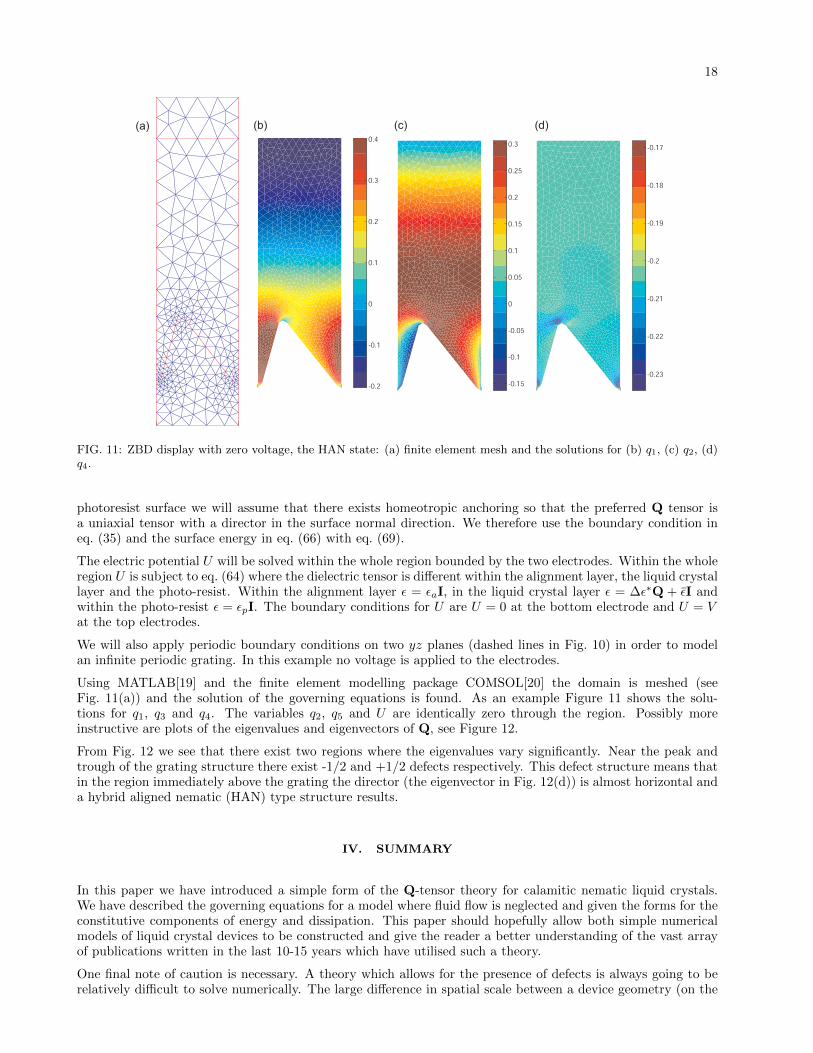
FIG. 11: ZBD display with zero voltage, the HAN state: (a) finite element mesh and the solutions for (b) q1, (c) q2, (d)q4.

photoresist surface we will assume that there exists homeotropic anchoring so that the preferred Q tensor isa uniaxial tensor with a director in the surface normal direction. We therefore use the boundary condition ineq. (35) and the surface energy in eq. (66) with eq. (69).

The electric potential U will be solved within the whole region bounded by the two electrodes. Within the wholeregion U is subject to eq. (64) where the dielectric tensor is different within the alignment layer, the liquid crystallayer and the photo-resist. Within the alignment layer ε = εaI, in the liquid crystal layer ε = ∆ε∗Q + εI andwithin the photo-resist ε = εpI. The boundary conditions for U are U = 0 at the bottom electrode and U = Vat the top electrodes.

We will also apply periodic boundary conditions on two yz planes (dashed lines in Fig. 10) in order to modelan infinite periodic grating. In this example no voltage is applied to the electrodes.

Using MATLAB[19] and the finite element modelling package COMSOL[20] the domain is meshed (seeFig. 11(a)) and the solution of the governing equations is found. As an example Figure 11 shows the solu-tions for q1, q3 and q4. The variables q2, q5 and U are identically zero through the region. Possibly moreinstructive are plots of the eigenvalues and eigenvectors of Q, see Figure 12.

From Fig. 12 we see that there exist two regions where the eigenvalues vary significantly. Near the peak andtrough of the grating structure there exist -1/2 and +1/2 defects respectively. This defect structure means thatin the region immediately above the grating the director (the eigenvector in Fig. 12(d)) is almost horizontal anda hybrid aligned nematic (HAN) type structure results.

IV. SUMMARY

In this paper we have introduced a simple form of the Q-tensor theory for calamitic nematic liquid crystals.We have described the governing equations for a model where fluid flow is neglected and given the forms for theconstitutive components of energy and dissipation. This paper should hopefully allow both simple numericalmodels of liquid crystal devices to be constructed and give the reader a better understanding of the vast arrayof publications written in the last 10-15 years which have utilised such a theory.

One final note of caution is necessary. A theory which allows for the presence of defects is always going to berelatively difficult to solve numerically. The large difference in spatial scale between a device geometry (on the

19

-0.23

-0.22

-0.21

-0.2

-0.19

-0.18

-0.17

-0.2

-0.15

-0.1

-0.05

0

0.05

0.15

0.2

0.25

0.3

0.35

0.4

(a) (d)(c)(b)

FIG. 12: ZBD display with zero voltage, the HAN state: the three eigenvalues (a), (b) and (c) and the eigenvectorassociated with the largest eigenvalue.

scale of 10s or 100s of microns) and the defect core (on the scale of 10s to 100s of nanometres) means thatdiscretisation of even a static example can lead to large numbers of numerical elements. A non-uniform gridis essential and, if the dynamic equations are to be solved, both adative meshing and timestepping will alsobe necessary. A number of papers have been written about these topics and those attempting to model suchsystems would be advised to consult these papers or seek assistance from researchers in the area[21–23].

[1] E. G. Virga, Variational theories for liquid crystals, Chapman & Hall, London (1994).[2] A. M. Sonnet and E. G. Virga, Dissipative Ordered Fluids: Theories for Liquid Crystals, Springerl, New York (2010).[3] L. A. Madsen, T. J. Dingemans, M. Nakata, and E. T. Samulski, Thermotropic biaxial nematic liquid crystals, Phys.

Rev. Lett. 92, 145505 (2004).[4] B. R. Acharya, A. Primak, and S. Kumar, Biaxial nematic phase in bent-core thermotropic mesogens, Phys. Rev.

Lett. 92, 145506 (2004).[5] G. R. Luckhurst, S. Naemura, T. J. Sluckin, S. K. Thomas, & S. S. Turzi, Molecular-field-theory approach to the

Landau theory of liquid crystals: Uniaxial and biaxial nematics, Phys. Rev. E 85, 031705 (2012).[6] N. Schophol and T. J. Sluckin, Defect core structure in nematic liquid crystals, Physical Review Letters 59, p.2582

(1987).[7] E. B. Priestley, P. J. Wojtowicz and P. Sheng, Introduction to liquid crystals, Plenum Press, New York and London

(1976).[8] H. Mori, E. C. Gartland, J. R. Kelly and P. J. Bos, Multidimensional director modeling using the Q tensor repre-

sentation in a liquid crystal cell and its application to the π cell with patterned electrodes, Jap. J. App. Phys. 38,p.135 (1999).

[9] D. W. Berreman and S. Meiboom, Tensor representation of Oseen-Frank strain energy in uniaxial cholesterics, Phys.Rev. A 30, p.1955 (1984).

[10] K. Schiele and S. Trimper, On the elastic constants of a nematic liquid crystal, Physica Status Solidi B 118, p.267(1983).

[11] A. L. Alexe-Ionescu, Flexoelectric polarisation and 2nd order elasticity for nematic liquid crystals, Phys. Lett. A180(6), p.456 (1993).

[12] R. Meyer, Piezoelectric effects in liquid crystals, Phys. Rev. Lett. 22, p.918 (1969).[13] P. G. de Gennes and J. Prost, The physics of liquid crystals, 2nd Edition, Clarendon Press, Oxford (1993).[14] G. Barbero, I. Dozov, J. F. Palierne and G. Durand, Phys. Rev. Lett. 56, p.2056 (1986).[15] M. A. Osipov, The order parameter dependence of the flexoelectric coefficients in nematic liquid-crystals, J. Phys.

Lett. (Paris) 45, p.L823 (1984).[16] M. A. Osipov and S. Hess, Density functional approach to the theory of interfacial properties of nematic liquid

crystals, Journal of Chemical Physics 99, p.4181 (1993).[17] C. V. Brown, G. P. Bryan-Brown, and J. C. Jones, U.S. Patent No. 6,249,332 19 June 2001.

20

[18] C. J. P. Newton and T. P. Spiller, Bistable Nematic Liquid-Crystal Device Modeling, in SID Proceedings of IDRC97, edited by J. Morreale SID, Santa Ana, CA, p.13 (1997).

[19] MATLAB version 8.1 (R2013a), The MathWorks Inc., Natick, Massachusetts (2013)[20] COMSOL Multiphysics, version 4.3b, COMSOL Inc. (2013)[21] A. Ramage and E. C. Gartland Jnr, A preconditioned nullspace method for liquid crystal director modelling, SIAM

Journal on Scientific Computing 35, p. B226 (2013).[22] C. S. MacDonald, J. A. Mackenzie, A. Ramage and C. J. P. Newton, Efficient moving mesh methods for Q-tensor

models of nematic liquid crystals, Strathclyde Mathematics Research Report No. 10 (2013).[23] MacDonald, C. S. MacDonald, J. A. Mackenzie, A. Ramage and C. J. P. Newton, Robust adaptive computation of a

one-dimensional Q-tensor model of nematic liquid crystals, Computers and Mathematics with Applications, 64(11),p. 3627 (2012).