4 Air demand modelling: overview and application to a ... · PDF fileAir demand modelling:...
32
4 Air demand modelling: overview and application to a developing regional airport M. Nadia Postorino University ‘Mediterranea’ of Reggio Calabria, Italy Abstract Air demand forecast at airports is an important problem for the airport management and also for the regulator that has to plan a homogeneous development of the overall transport system. The current tendency is towards airport privatization; then, the goal to increase the served demand is one of the most important together with the progress of non-aviation activities. The evolution of the air transport system both in terms of low-cost companies, that generally use regional airports, and new technologies (as regional jets) has given a further impulse to the development of planning methodologies able to support decisions for an efficient distribution of resources. Regional airports can play an important role in this new background if the most suitable developing strategies are identified. This chapter wants to give a general overview about the problem of the air demand modelling, both in terms of theoretical approaches and practical problems. Models are classified with respect to different criteria, and the most suitable models for each planning level are also identified. An application to a regional airport in Southern Italy is also presented in order to test some of the described approaches and to obtain practical indications about applied models and developing strategies to be used. Keywords: air demand; air demand model classification; airport catchment area; time series models; random utility models. 1 Introduction The estimate of transport demand has always been one of the most important stages in the transport system planning process and one of the most stimulating challenges for the analysts, because the dependence of demand on the overall www.witpress.com, ISSN 1755-8336 (on-line) WIT Transactions on State of the Art in Science and Engineering, Vol 38, © 2010 WIT Press doi:10.2495/978-1-84564-143-6/04
Transcript of 4 Air demand modelling: overview and application to a ... · PDF fileAir demand modelling:...
4
Air demand modelling: overview and application to a developing regional airport
M. Nadia Postorino University ‘Mediterranea’ of Reggio Calabria, Italy
Abstract
Air demand forecast at airports is an important problem for the airport management and also for the regulator that has to plan a homogeneous development of the overall transport system. The current tendency is towards airport privatization; then, the goal to increase the served demand is one of the most important together with the progress of non-aviation activities. The evolution of the air transport system both in terms of low-cost companies, that generally use regional airports, and new technologies (as regional jets) has given a further impulse to the development of planning methodologies able to support decisions for an efficient distribution of resources. Regional airports can play an important role in this new background if the most suitable developing strategies are identified. This chapter wants to give a general overview about the problem of the air demand modelling, both in terms of theoretical approaches and practical problems. Models are classified with respect to different criteria, and the most suitable models for each planning level are also identified. An application to a regional airport in Southern Italy is also presented in order to test some of the described approaches and to obtain practical indications about applied models and developing strategies to be used.
Keywords: air demand; air demand model classification; airport catchment area; time series models; random utility models.
1 Introduction
The estimate of transport demand has always been one of the most important stages in the transport system planning process and one of the most stimulating challenges for the analysts, because the dependence of demand on the overall
www.witpress.com, ISSN 1755-8336 (on-line) WIT Transactions on State of the Art in Science and Engineering, Vol 38, © 2010 WIT Press
doi:10.2495/978-1-84564-143-6/04
78 DEVELOPMENT OF REGIONAL AIRPORTS socio-economic system (particularly, income and job activities on the territory) makes it difficult to obtain reliable values. On the other hand, the supply characteristics (as e.g. terminal capacity, parking size and runways in the case of an airport system) as well as their performances and profitability are strongly dependent on the predicted demand levels.
Significant overestimates or underestimates of future demand levels lead to wrong developing policies that can generate respectively: (a) uneconomic use of infrastructures and/or services; (b) quick worsening of the transport system performances due to infrastructures and/or service deficiencies compared with the actual demand levels.
Generally, the analysis and the simulation of an air transport system concern three macro-topics:
● estimate of the air transport demand and its distribution among several competitive airports;
● identification of the supply organization and its effects on the different actors (community, passengers, airports, airlines);
● forecast of the air transport services and their induced effects on the air demand as well as on the other actors working in the system.
The first two aspects are linked to the system simulation for a given scenario (current scenario or future hypotheses). The third aspect depends on the airline/airport decision policies, the profit analysis, the market conditions, and, last but not least, the political decisions aiming at the system development following social other than technical criteria.
The increase in the air transport demand in the last few decades, also helped by the deregulation policy, has had a major effect of increasing transport services offered by different air carriers and has resulted in increasing congestion levels both in the airways and at airports (Graham and Guyer [1]). As an immediate effect of deregulation, the service offered to users, in terms of trip organization and costs, has changed rapidly and various alliances and mergers have occurred, together with the emergence of new air carriers in the market. For users, deregulation has produced greater benefits due to airfare decrease and the opportunity to choose among more flights supplied by more air carriers (Cohas et al. [2]). Thanks to deregulation, various air carriers have the opportunity to offer their services along high-demand routes, new connections have arisen and fare reductions have been applied (ATAG [3]). Hence, there has been an increase in the demand level, especially for non-systematic reasons (e.g. in Europe a reduction of 15% in airfares has produced an increase of about 10% in the carried passengers, Italian Ministry of Transport [4]).
Demand variations depending on local aspects (such as the building of a new airport or the expansion of an existing one) represent another important factor in modelling air transport demand, as the use of hub-and-spoke systems means that each pole can be potentially connected to almost any other.
Air transport demand directly affects the planning of airport terminals in terms of ground services design (check-in/check-out points, waiting areas, facilities as restaurants, shops and so on). In order to properly design such areas,
www.witpress.com, ISSN 1755-8336 (on-line) WIT Transactions on State of the Art in Science and Engineering, Vol 38, © 2010 WIT Press

AIR DEMAND MODELLING 79
both the absolute demand and its temporal distribution are required. Furthermore, even the competitiveness among airlines plays an important role to define the demand distribution.
The above considerations show how important the demand characteristic analysis and its evolution in time are in order to design more effectively the service supplied by both airport managers and air carriers.
Reliability of the demand estimates depends on the kind of model and data availability. Models theoretically efficient in terms of forecast often require a lot of data referred to users and both socio-economic and supply systems for a long period of time in order to estimate not only the current demand characteristics but also the future levels. The knowledge of current and future levels helps planners to develop effective short-medium and long-term actions, respectively.
Thus, data availability and model reliability are the two key elements to obtain high-quality demand level forecast, within the effectiveness limits defined by the stability of the boundary conditions. The latter can be identified in the socio-economic and political stability, which has a relevant influence on the user’s decisions to make trips and particularly to travel by aircraft.
In the following, the relationship between demand and airport catchment area is discussed (Sections 2), and a classification of the air demand approaches with respect to different criteria is proposed together with a description of the two most important air demand approaches (Section 3). Finally, after an overview of the Italian airport system (Section 4) an application to a regional airport located in Southern Italy is presented and discussed (Section 5).
2 Demand modelling and airport catchment area
A key element for evaluating the developing potentiality of airport systems, particularly regional airport systems, is the demand forecast for each airport serving the considered region; such a forecast should be consistent with the airport choices made by the air users travelling from and towards the region itself.
As it is well-known to transport analysts, demand forecast is a relevant input for the transport system planning; particularly, in the case of a regional airport, system forecasts of demand have a significant influence on the future functioning of each airport as well as on the development of the airport master plans.
Generally speaking, a demand model is a mathematical relationship linking the expected demand level (dependent variable) to one or more explanatory variables (independent variables), whose nature depends on the kind of model and the availability of the corresponding data.
The choice to start the air trip from a given airport can depend on many factors as accessibility, facilities, air services and connectivity levels (i.e. the destinations that can be reached from the airport itself). Accessibility depends on the land network available on the region, while the other factors depend on the airport characteristics and the airline supply.
www.witpress.com, ISSN 1755-8336 (on-line) WIT Transactions on State of the Art in Science and Engineering, Vol 38, © 2010 WIT Press
80 DEVELOPMENT OF REGIONAL AIRPORTS
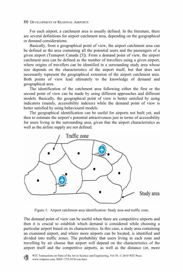
For each airport, a catchment area is usually defined. In the literature, there are several definitions for airport catchment area, depending on the geographical or demand considerations.
Basically, from a geographical point of view, the airport catchment area can be defined as the area containing all the potential users and the passengers of a given airport (Transport Canada [5]). From a demand point of view, the airport catchment area can be defined as the number of travellers using a given airport, where origins of travellers can be identified in a surrounding study area whose size depends on the characteristics of the airport itself, but that does not necessarily represent the geographical extension of the airport catchment area. Both points of view lead ultimately to the knowledge of demand and geographical area.
The identification of the catchment area following either the first or the second point of view can be made by using different approaches and different models. Basically, the geographical point of view is better satisfied by using indicators (mainly, accessibility indexes) while the demand point of view is better satisfied by using behavioural models.
The geographical identification can be useful for airports not built yet, and then to estimate the airport’s potential attractiveness just in terms of accessibility for users living in the surrounding area, given that the airport characteristics as well as the airline supply are not defined.
Figure 1: Airport catchment area identification: Study area and traffic zone.
The demand point of view can be useful when there are competitive airports and then it is crucial to establish which demand is considered while choosing a particular airport based on its characteristics. In this case, a study area containing an examined airport, and where more airports can be located, is identified and divided into traffic zones. The probability that users living in each zone and travelling by air choose that airport will depend on the characteristics of the airport itself and the competitive airports, as well as the distance (or, more
www.witpress.com, ISSN 1755-8336 (on-line) WIT Transactions on State of the Art in Science and Engineering, Vol 38, © 2010 WIT Press

AIR DEMAND MODELLING 81
generally, the accessibility measures) between each traffic zone and the examined airport [6, 7, 8, 9]. Then, the demand obtained at each airport represents the catchment area from the demand point of view, while its geographical identification potentially corresponds to the study area (Figure 1). Furthermore, a distinction can be made between primary and secondary airport catchment areas (Transport Canada [5]). For a given airport, the first one refers to air travellers choosing that airport because they are ‘captive’. The second one refers to air travellers that may choose that airport but are not captive and then are more elastic with respect to the choice of another airport (Figure 2). Generally, the secondary catchment area is typical both for airports where there are low-cost airlines and for classes of users that are more price-sensitive.
Figure 2: Primary and secondary airport catchment area.
Whatever be the approach, the knowledge of the airport catchment area is important because it represents the possible demand for the airport and then the potential for airport development. Demand levels and airport catchment area are then highly dependent on each other and land accessibility plays an important role.
As it is well-known in the economic and social sciences, accessibility is the key to development and particularly for airports. In fact, the larger the catchment area the larger the potential demand at the airport. An important factor for a successful airport development, mainly for regional airports, is to increase the catchment area other than providing good services in terms of fares, destinations and frequencies.
The simplest method to identify the geographical extension of the catchment area is to define a threshold value with reference to one or more accessibility indexes: the geographical area whose accessibility index is less than the threshold value is the airport potential catchment area; in other words, it contains the potential users and passengers of the airport. On a first approximation, the catchment area can be identified as the geographical area not larger than a
www.witpress.com, ISSN 1755-8336 (on-line) WIT Transactions on State of the Art in Science and Engineering, Vol 38, © 2010 WIT Press

82 DEVELOPMENT OF REGIONAL AIRPORTS prefixed time value (as 2 hours by car, for some important European airports (van Reeven, de Vlieger and Karamychev [10]) or 60 minutes by any land vehicles in the USA (Milone et al. [11])).
The knowledge of the geographical origin of passengers is a useful piece of information for the airport management in order to identify the best developing strategies; for example to decide if it is more suitable to invest on land accessibility rather than on airport facilities and services. Such knowledge can be achieved by running sample surveys on departing air travellers at the airport.
The key elements that can play an important role for the development of an airport can be identified as:
● capability to generate demand in the airport catchment area; ● capability to generate adequate demand (from the point of view of economic
convenience) for potential point-to-point links; ● capability to adapt the airport services to the need and exigencies of the
airlines; ● involvement of airlines on airport investments to improve the offered
services.
In terms of factors affecting the size of the airport catchment area, and with reference to the primary catchment area only, the most relevant are:
● living population; ● yearly average income and average family income; ● employment level; ● sector of employment.
Generally, if the first three factors increase, the number of air travellers increases (and then the catchment area); while the distribution of sectors of employments is a useful indication to identify the potential air travellers by trip purpose (e.g. business travellers).
Furthermore, the airport catchment area also has an important impact on the financial situation of the airport itself. For example, airports surrounded by densely populated catchment areas and increasing population with employment levels and income in the average or over the average and employment sectors that generate business trips, generally, have got positive financial situations. An important role is also played by competition among airports; airports far away from the main national airports (250 kilometres following some studies on the Canadian regional airports [5]), where there are low-cost airlines, and that are also at a proper distance from the potential competing airport (e.g. 90 minutes by car) have still a good financial situation. On the other hand, airports offering similar services and sharing the same catchment area within a radius of about 100 kilometres, probably will have both a critical and negative financial situation.
The airport development also depends on the location of other, potentially competitive, airports. In the current situation, airports play a competitive role rather than a cooperative one and then the distance among airports as well as the
www.witpress.com, ISSN 1755-8336 (on-line) WIT Transactions on State of the Art in Science and Engineering, Vol 38, © 2010 WIT Press
AIR DEMAND MODELLING 83
services offered are crucial in terms of user choices. Generally, users are willing to cover longer distances to obtain better trip fares, point-to-point flights, larger choice sets of available airlines and flights to choose the best options in terms of departure time, destination and airline reliability (Suzuki [12]).
Furthermore, the presence of fast land modes (as fast trains) that can be competitive in terms of fares and times with respect to the destinations served at the airports can be an additional important factor in the airport users’ choice. Indeed, one of the EU topics of major interest is the analysis of the fast train network influence on the distribution of traffic volumes among airports; land fast links between city pairs are supposed to produce a decrease in the air transport demand among the same city pairs (Button [13]). However fast trains also represent an easy way to arrive quickly at major airports (e.g. the Inter City Express links between Frankfurt and Paris or the international high speed trains linking Paris and Brussels to Great Britain trough the Channel Tunnel) and then they also contribute to improve the airport catchment area in a whole, integrated and inter-modal transport system. The complexity of the fast train role (competition or integration?) with respect to airports is one of the most attractive research fields in the transport system analysis.
3 Demand model classification
Passengers demand models can be classified with reference to the transport system representation, the mathematical formulation, the nature of variables (Table 1).
Table 1: Demand model classification.
Multi-mode models
Stage models (discrete choice)
Competitive Static models Non-competitive Uni-mode models
Stage models (discrete choice)
Competitive
Zone approach
Time series models Non-competitive Competitive Static models Non-competitive Uni-mode models
Competitive
Airport pairs approach
Time series models Non-competitive
First of all, a distinction can be made between air demand models providing forecasts for specific city-pairs, corresponding to airport-pairs serving those cities, and demand models providing forecasts for O–D pairs, corresponding to traffic zones pairs. Whatever be the used approach, in the first case the focal point is the analysis of the specific relationship between airports or among one
www.witpress.com, ISSN 1755-8336 (on-line) WIT Transactions on State of the Art in Science and Engineering, Vol 38, © 2010 WIT Press

84 DEVELOPMENT OF REGIONAL AIRPORTS airport and all the others, while in the second case the demand model is usually part of a more general framework where demand is estimated for traffic zones and many transport modes; for the aircraft mode, demand is also allocated to one or more competitive airports by using suitable models (airport choice is described in Chapter 5).
Traditionally, demand models are classified as aggregate and disaggregate depending on the nature of data referred to demand and explanatory variables. If the variable ‘demand’ is referred to a single user, and so the explanatory variables, the model is said to be disaggregate, while if the variable ‘demand’, and then the explanatory variables, are referred to a homogeneous group of users the model is said to be aggregate.
Furthermore, models can be called: (1) descriptive or behavioural according to whether there are or not explicit hypotheses about trip user behaviour; (2) multi-mode or uni-mode if they allow obtaining mode shares among several alternative modes or demand on only one transport mode, respectively. Particularly, multi-mode models refer to the simulation of the overall transport system, where many transport modes are generally available (e.g. train, bus, car, aircraft), and then the demand on many transport modes can be computed. On the contrary, uni-mode models provide forecasts of demand for only one transport mode and then they are suitable for the simulation of a part of the overall transport system (e.g. the air transport system).
Multi-mode models are generally stage models, where more trip characteristics as destination, frequency, mode and so on can be simulated by using discrete choice models (a general overview is in [14, 15]).
Uni-mode models can be classified as static if they simulate air demand at a given time, time series if they simulate the demand trend for a given time period, or stage models if they simulate more trip characteristics but for a mode-specific demand.
Time series models can still be grouped as Simple Time Series (or univariate) and Causal Modelling (or multivariate). Simple Time Series approaches, among the most used to obtain air demand forecasts, consider the stochastic nature of an event does not vary in time and they simulate the demand trend without explaining the causes. In other words, explanatory variables are not considered. On the other hand, Causal Modelling models simulate demand in terms of cause-effect relationships, i.e. they associate explanatory variables to the observed demand by means of mathematical relationships linking independent variables (causes) to dependent variables (effects). Explanatory variables are generally referred to the examined mode, but characteristics of alternative modes (and, particularly, competitive modes as fast train with respect to aircraft) can also be considered by using suitable variables (mainly, level-of-service variables). From this point of view, uni-mode models can be classified, respectively, as non-competitive and competitive.
Demand forecast can be achieved at two different levels of detail: for long-term planning (strategic level) and for medium-short planning (tactical or operational level), where the difference is mainly due to the amount of required input data and the resulting level of output information.
www.witpress.com, ISSN 1755-8336 (on-line) WIT Transactions on State of the Art in Science and Engineering, Vol 38, © 2010 WIT Press
AIR DEMAND MODELLING 85
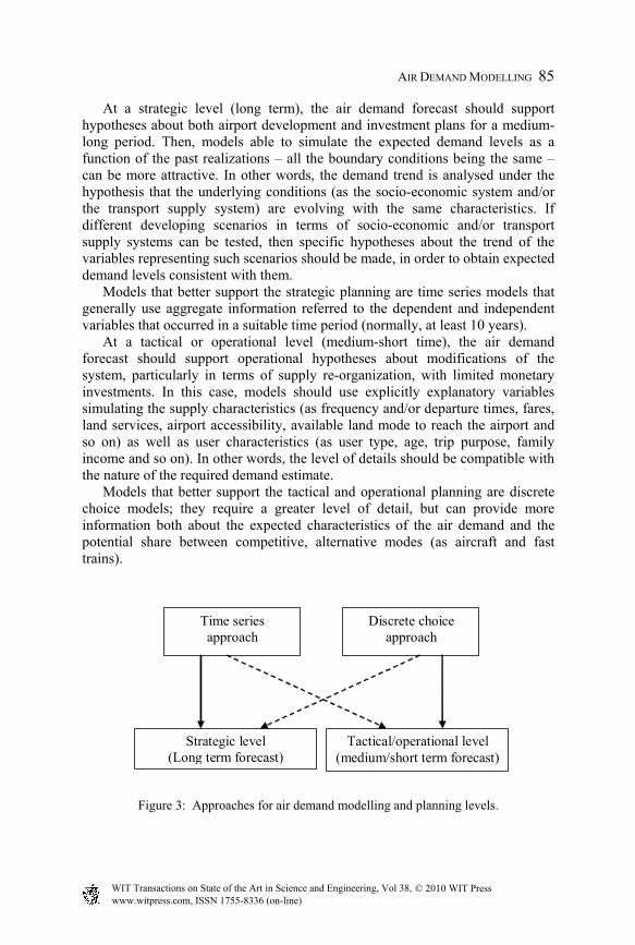
At a strategic level (long term), the air demand forecast should support
hypotheses about both airport development and investment plans for a medium-long period. Then, models able to simulate the expected demand levels as a function of the past realizations – all the boundary conditions being the same – can be more attractive. In other words, the demand trend is analysed under the hypothesis that the underlying conditions (as the socio-economic system and/or the transport supply system) are evolving with the same characteristics. If different developing scenarios in terms of socio-economic and/or transport supply systems can be tested, then specific hypotheses about the trend of the variables representing such scenarios should be made, in order to obtain expected demand levels consistent with them.
Models that better support the strategic planning are time series models that generally use aggregate information referred to the dependent and independent variables that occurred in a suitable time period (normally, at least 10 years).
At a tactical or operational level (medium-short time), the air demand forecast should support operational hypotheses about modifications of the system, particularly in terms of supply re-organization, with limited monetary investments. In this case, models should use explicitly explanatory variables simulating the supply characteristics (as frequency and/or departure times, fares, land services, airport accessibility, available land mode to reach the airport and so on) as well as user characteristics (as user type, age, trip purpose, family income and so on). In other words, the level of details should be compatible with the nature of the required demand estimate.
Models that better support the tactical and operational planning are discrete choice models; they require a greater level of detail, but can provide more information both about the expected characteristics of the air demand and the potential share between competitive, alternative modes (as aircraft and fast trains).
Time series approach
Discrete choice approach
Strategic level (Long term forecast)
Tactical/operational level (medium/short term forecast)
Figure 3: Approaches for air demand modelling and planning levels.
www.witpress.com, ISSN 1755-8336 (on-line) WIT Transactions on State of the Art in Science and Engineering, Vol 38, © 2010 WIT Press

86 DEVELOPMENT OF REGIONAL AIRPORTS However, time series models and discrete choice models can be used at both planning levels (Figure 3), depending on the nature of the analysis and the data availability as well as the required output detail levels.
For example, discrete choice models can be used to test hypotheses about the development of the overall transport system, the air transport system being only a part of it, in relation to long-term planning projects as the building of fast speed railways or new road infrastructures. Similarly, time series models can be used to verify airport developing policies; for example the introduction of new links or variations in flight frequencies, for short term periods as 2–5 years.
Model development
Model identification
Model application
Model choice
Function identification
Relevant variables
identification
Model calibration
Function Relevant variables
Model parameters
Model check
Relevant variables data
base
Model application
Planning level: • Strategic • Tactical
Figure 4: Model development and application.
www.witpress.com, ISSN 1755-8336 (on-line) WIT Transactions on State of the Art in Science and Engineering, Vol 38, © 2010 WIT Press

AIR DEMAND MODELLING 87
Forecast of the air transport demand can also be referred both to a single airport inside a geographical (or administrative) region and to a set of airports inside a common area where they can be considered ‘competitive’ to each other. The choice to simulate the air demand only for one airport or to verify its distribution among two or more of them depends on the effective competition among airports, strongly linked to the identification of the airport catchment area.
Whatever be the planning level, the development and application of an air demand model requires three main steps (see also Figure 4):
● identification of the most suitable mathematical model able to simulate/forecast air transport demand with respect to the expected results and/or the prefixed goals;
● availability of data to calibrate the model parameters and to apply the model; ● check of the obtained model.
In the application stage, an available model can be used to simulate the air demand, the only care being the opportunity to use model parameters referred to similar socio-economic contexts. In this case, the check stage concerns the application of the model to a known situation in order to verify the congruence of the parameters, while in the case of model development the check stage refers to some statistical tests about the goodness of the estimated parameters and the statistical reliability of the overall model.
One important aspect concerning both the development and application of an air demand model is the data collection. Data referred to (air) transport demand concerning both user socio-economic characteristics and travel behaviour are often difficult to obtain. Generally, available data refer to official, aggregate statistics on boarded/de-planed passengers, pro-capita income for geographical/administrative regions and so on, but depending on the kind of model and detail required they can be inadequate to develop a suitable demand model.
Moreover, travel times and costs are the most relevant level-of-service variables introduced in a demand function. For air transport systems, travel times refer to flight duration, possible waiting time for connecting flights, boarding/ disembarkation, baggage claim, and access/egress times. Costs mainly refer to monetary costs and generally to airfare.
Some data concerning airline supply can be difficult to obtain without specific surveys; particularly, airfare is the most difficult variable to quantify for at least two main reasons: (1) useful data are not always available and (2) there is a very large set of fares proposed by different air carriers and also inside the same air carrier. Actually, airfares can change significantly depending on many factors as the day on which the ticket is bought, the time period (week-end, particular days or months of the year and so on), the number of booked people, the age, the participation to flight programs (as frequent flier programs) and so on. When international trips are considered, the problem is still more complex because origins and/or destinations are in different countries with different currencies, while the fare has to be expressed in one reference monetary value, e.g. by using the exchange rate that, in turn, is variable during the year.
www.witpress.com, ISSN 1755-8336 (on-line) WIT Transactions on State of the Art in Science and Engineering, Vol 38, © 2010 WIT Press

88 DEVELOPMENT OF REGIONAL AIRPORTS
− j
To overcome the problem by considering the quality of the offered service (and then, implicitly, the willingness to pay to use it), the hedonic pricing theory can be used (Rosen [16]). Its basic foundations are that users evaluate the characteristics of a good or the services it offers rather than the good itself. Following this approach, the observed fare can be considered as a function of the offered service and/or user characteristics; then, users are willing to pay according to the satisfaction they receive.
The following sections provide a brief overview of the main characteristics for both time series and discrete choice models.
3.1 Time series approach
Time series models to simulate air transport demand can have different levels of complexity depending on the general aims and the data availability for both model calibration and application. They have been largely used to predict air demand levels, see among others [17, 18, 19, 20, 21, 22, 23].
To briefly summarize, a time series is a stochastic process where the time index takes on a finite or countable infinite set of values. A stochastic process is an ordered and infinite sequence of random variables: if the time index t assumes only integer values, then it is a discrete stochastic process. To describe it, its mean and its variance are used as well as two functions: the AutoCorrelation Function (ACF) ρk, k being the lag, and the Partial AutoCorrelation Function (PACF) πk, k being the lag. The ACF is a measure of the correlation between two variables composing the stochastic process, which are k temporal lags far away; the PACF measures the net correlation between two variables which are k temporal lags far away [24, 25].
AutoRegressive Moving Average (ARMA) models are a class of stochastic processes expressed as follows:
1 1
,−= =
− = −∑ ∑p q
t i t i t j ti j
X X a aφ θ (1)
where at is a White Noise process, φ and θ the model parameters, p and q the order of the AutoRegressive (AR) and Moving Average (MA) processes, respectively [24]. If the B operator such as Xt–1 = BXt is introduced, the general form of an ARMA model can be written as follows:
( ) ( ) .⋅ = ⋅t tB X B aφ θ
To estimate these models, some conditions should be verified: the series must be stationary and ACF and PACF must be time-independent. The non-stationarity in variance can be removed if the series is transformed with the logarithmic function. The non-stationarity in mean can be removed by using the operator ∇ = (1–B) applied d times in order to make the series stationary. In this way, the ARMA model becomes an ARIMA (AR Integrated MA) model:
( ) ( ) .∇ ⋅ = ⋅dtB X B aφ θ t (2)
www.witpress.com, ISSN 1755-8336 (on-line) WIT Transactions on State of the Art in Science and Engineering, Vol 38, © 2010 WIT Press

AIR DEMAND MODELLING 89
This family of univariate models is largely used to obtain air demand prediction at a first level of knowledge and when no more data other than the demand time series is available. In this case, Xt represents the air demand at an airport i (or for an origin/destination pair i, or a traffic zone i) at time t, dit:
( ) ( ) .∇ ⋅ = ⋅dit tB d B aφ θ
For a given set of data, the Box-Jenkins approach [24] is the most known method to find an ARIMA model that effectively can reproduce the data generating the process. The method requires three stages: identification, estimation and diagnostic checking.
Preliminarily, data analyses should be carried out in order to verify the presence of outliers. The identification stage provides an initial ARIMA model specified on the basis of the estimated ACF and PACF, starting from the original data:
● If the autocorrelations decrease slowly or do not vanish, there is non-stationarity and the series should be differenced until stationarity is obtained. Then, an ARIMA model can be identified for the differenced series.
● If the process underlying the collected series is a MA(q), then the ACF ρk is zero for k > q and the PACF is decreasing.
● If the process underlying the collected series is an AR(p), then the PACF πk is zero for k > p and the ACF is decreasing.
● If there is no evidence for a MA or an AR then a mixture ARMA model may be adequate.
Several statistical tests have been developed in the literature to verify if a series is stationary, among these, the most widely used is the Dickey-Fuller test (Makridakis et al. [26]). After an initial model has been identified, the AR and MA parameters have to be estimated, generally by using least squares (LS) or maximum likelihood (ML) methods. The choice of the AR component order derives from the analysis of the PACF correlogram; for large sample size, if the order of the AR component is p, the estimate of the partial autocorrelations πk are approximately normally distributed with mean zero and variance 1/N for k > p, where N is the sample size. The significance of the residual autocorrelations is often checked by verifying if the obtained values are within two standard error bounds, ±2/√N, where N is the sample size (Judge et al. [25]). If the residual autocorrelations at the first N/4 lags are close to the critical bounds, the reliability of the model should be verified. Another test that can be used is the Ljung and Box one [27]:
1 2ˆ
1
( 2) ( ) [ ( )]−
=
= ⋅ + ⋅ − ⋅∑m
ak
Q N N k kN ρ ,
where ˆ ( )a kρ are the autocorrelations of the estimate residuals and k is a prefixed number of lags. For an ARMA (p, q) process this statistic is approximately χ2
www.witpress.com, ISSN 1755-8336 (on-line) WIT Transactions on State of the Art in Science and Engineering, Vol 38, © 2010 WIT Press

90 DEVELOPMENT OF REGIONAL AIRPORTS distributed with (k–p–q) degrees of freedom if the orders p and q are specified correctly.
To check the residuals normality, the Jarque-Bera (JB) test [28] can be used:
( )22 3
JB ,6 4
⎛ ⎞− −⎜ ⎟= ⋅ +⎜ ⎟⎝ ⎠
pN n KS
where S is a measure of skewness, K is a measure of Kurtosis, np is the number of parameters and N is the sample size. This test verifies if skewness and kurtosis of the time series are different from those expected for a normal distribution. Under the null hypothesis of normal distribution, the JB test is approximately χ2 distributed with two degrees of freedom.
Models (1) or (2) use the past values of the examined variable to predict its future values. If some explanatory (or independent) variables are inserted in order to verify cause-and-effect relationships, the dependent variable Xt generally depends on lagged values of the independent variables and the model can be said multivariate. The length of the lag may sometimes be known a priori, but usually it is unknown and in some cases it is assumed to be infinite.
The simplest multivariate time series demand models are of the kind as follows:
0 ,= + +Tit it itd β y uβ
, 1 ,−= +it i t itu uρ ε
where demand for an airport i (or for an origin/destination pair i, or a traffic zone i) at time t, dit, is specified as function of n explanatory (and relevant) variables yit. βT are the unknown model parameters, β0 the model constant, uit a random term, εit a White Noise random residual and ρ the autocorrelation parameter taking into account the time dependence among the variables. The basic hypothesis is that the variable at year t is a function of the same variable at year t–1, as specified by the random term.
More general models can be obtained by starting from univariate ARIMA models and introducing more explanatory variables. Normally, if one dependent variable and one explanatory variable are considered, then the model has the form as follows:
0 1 , 1 , ,− −= + + + + +…it it i t P i t P itd y y y eα β β β (3)
under the hypothesis that βk = 0 for k greater than a finite number P, called lag length. Models (3) are called finite distributed lag models, because the lagged effect of a change in the independent variable is distributed into a finite number of time periods.
If e ~ (0, σ2I) and yt are fixed, then, based on the sample information, the LS estimator is the best linear unbiased estimator for (α, β0, …, βP). If the true lag length P is unknown but an upper bound M is known, then the LS estimator of β’ = (α, β0, β1, …, βM)T is inefficient since it ignores the restrictions βP+1 = … =
www.witpress.com, ISSN 1755-8336 (on-line) WIT Transactions on State of the Art in Science and Engineering, Vol 38, © 2010 WIT Press

AIR DEMAND MODELLING 91
i
βM = 0. In order to compute P, these sequential hypotheses can be set up as follows:
1 2( , ,..., ) ( ),o n o id k k k n p k= Π
versus 1 2
1 0 0 0: 1, 0 , ,....,m mM ma P M m 1H H H Hβ −− += − + ⇒ ≠ .
The null hypotheses are tested sequentially beginning from the first one. The testing sequence ends when one of the null hypotheses of the sequence is rejected for the first time. The likelihood ratio statistic to test the m-th null hypothesis can be written as follows:
12
1
SSE SSE,
ˆ− −
− +
−= M m M m
mM m
λσ
+
where SSEP is the sum of the squared errors for a model with lag length P. This statistic has an F-distribution with 1 and (T – M + m – 3) degrees of freedom if
10H , 2
0H , 0mH are true.
When the lag has been computed, the explanatory variable can be inserted in the univariate model, in order to derive a so-called multivariate ARIMAX model. In the general case of more than one explanatory variables, the model has the form as follows:
(4) 1 2
(1) (1) (2) (2), ,
0 0( ) ( ) ........− − − −
= =
∇ Φ ⋅ = ⋅ + + +∑ ∑P P
dit t t t l i t l t l i t l
l lB d B a y yθ β β
where: ( )−j
t ly is the j-th independent variable at time (t–l) and ( )−j
t lβ is the corresponding parameter.
Figure 5 shows the different kinds of applications of air demand time series models, preferably for strategic planning levels.
Univariate models do not require explanatory variables but only the demand past ‘history’; furthermore, they do not require the explicit identification of the airport catchment area but, for example, only boarded/de-planed passengers at the airport, time series data being available.
On the other hand, multivariate models present one or more explanatory variables as frequencies, income, number of employment and so on; some of them, as socio-economic variables, refer to the airport catchment area that has to be explicitly identified.
As Figure 5 shows, univariate and multivariate models can be used at aggregate and disaggregate levels; in the last case, the variables are defined for each traffic zone, demand generated by each traffic zone at year t can be estimated and then characterized as function of destination, departure time, transport mode and so on, by using discrete choice models (Section 3.2). Furthermore, mode-specific travel demand (as air demand) can be directly
www.witpress.com, ISSN 1755-8336 (on-line) WIT Transactions on State of the Art in Science and Engineering, Vol 38, © 2010 WIT Press

92 DEVELOPMENT OF REGIONAL AIRPORTS generated for each traffic zone, and again the other characteristics as destination and departure time as well as airport, airlines, access mode are simulated.
Disaggregated level
Univariate and multivariate time series
models
Traffic zones
Discrete choice models
Predicted demand level for each traffic zone
at time t
Predicted demand level for each traffic zone
and given characteristics at time t
Time series demand
Univariate time series models
Predicted demand levels at the airport or for airport pairs
Multivariate time series models
Airport catchment area
Predicted demand levels at the airport or for airport pairs
Dependent and independent variables time series
Demand time series at airport or
for airport pairs
Aggregated level
Figure 5: Application of time series models to estimate air travel demand.
3.2 Discrete choice models
Discrete choice models are a well-known class of models largely used in the transportation field to obtain trip demand specified with some characteristics as trip purpose, trip origin and destination, departure time, transport mode and so on [14, 15]. The most general form of a discrete choice multistage demand model is:
(5) 1 2( , ,..., ) ( ),o n o id k k k n p k= Π i
where do(k1, k2,…, kn) is the travel demand with trip origin o and characteristics k1, k2, …, kn that can be specified from time to time depending on the exigencies; no is the number of potential users in the origin o and p(ki) is the choice percentage referred to the characteristic (or choice dimension) ki. They can be estimated by using simple statistical approaches or Random Utility Models (RUM).
www.witpress.com, ISSN 1755-8336 (on-line) WIT Transactions on State of the Art in Science and Engineering, Vol 38, © 2010 WIT Press

AIR DEMAND MODELLING 93
To estimate the air demand by starting from model (5), suitable choice
dimensions ki and the corresponding p(ki)s should be identified, as in the following simple sequential specification:
[ ] [ ] [ ]( , ) ( ) SE,TS ( / ) SE,TS ( / ) SE,TS= ⋅ ⋅odh od s m d sh p d osh p m odsh (6)
where SE and TS represent the vector of the socio-economic and territorial system characteristics, because the choice percentages depend on both user (socio-economic) and level-of-service/activity (territorial system) characteristics. Indexes o, d, h, s, m represent the trip dimensions, respectively, trip origin, trip destination, time period, trip purpose, trip travel mode, while p(./..)s represent the choice probability (or choice percentage) for each choice dimension.
As models (6) shows, the order in the sequence also defines the dependence of each choice dimension on the previous one by means of suitable variables; the identification of the more suitable sequence is not a trivial task; particularly, for mode-related choices it is not easy to identify the best and more reasonable sequence to model the complex user behaviour concerning travel planning. For example, the choice to travel by aircraft implies also the choices of departure and arriving airports, the airport access/egress mode, the airline (e.g. traditional vs. low-cost); the latter can be simulated by means of suitable variables inside the mode choice dimension or within a decision process where the choice dimensions, their hierarchical order, if any, and their reciprocal effects should be simulated (more on airport choice is in Chapter 5).
In any case, the sequence (6) might be completely changed if the user choice process happens in a different way, e.g. users travelling for leisure, first of all, can decide to use an aircraft to start their trip and then make all the other mode-related choices, included the trip destination. On the other hand, if destination is compulsory (e.g. business travel), sequence (6) matches the decision process. In any case, the identification of the best sequence and then the best model is the result of a trial-and-error procedure.
Sequential discrete choice models as in eq. (5) have been used at national level to simulate the trip demand on many available transport modes, included aircraft, so as to define the best developing policies for the overall transport system by taking into account also its impact. This approach could be particularly useful to verify how much the overall transport system and each of its components are responsible for the greenhouse effects and which actions could be undertaken in order to satisfy the Kyoto protocol.
The hypotheses underlying a RUM approach to estimate the p(./..)s suppose users are rational decision makers and they choose the best option among a set of available alternatives; such a choice is based on the random utility value associated to each alternative belonging to the choice set and depending on the characteristics (attributes) of the alternative itself and the other available alternatives. Then, users choose the option with the highest value of utility, and since utility is a random variable only the probability that users choose a specific alternative can be computed.
Starting from these hypotheses, many multistage RU discrete choice demand models can be identified by specifying choice dimensions, choice sequences and
www.witpress.com, ISSN 1755-8336 (on-line) WIT Transactions on State of the Art in Science and Engineering, Vol 38, © 2010 WIT Press

94 DEVELOPMENT OF REGIONAL AIRPORTS discrete choice models (Figure 6); whatever be the discrete choice model, its use requires: (1) the identification of the choice set; (2) the identification of the relevant attributes characterizing each alternative; (3) the identification of the mathematical form for the random utility variable [8, 29, 30, 31].
Figure 6: Steps in the discrete choice approach.
RUMs are a family of behavioural models trying to simulate user behaviour starting from some mathematical hypotheses. Recently, other paradigms have been proposed to understand user preferences, by using Neural Networks (NN) and fuzzy-NN approaches [32, 33, 34]. However, NN do not allow the explicit values of the parameters to be computed, so the interpretation of the model in terms of elasticity values, parameter ratios and so on cannot be obtained.
Estimation of the air demand requires more than the mode dimension because subsequent, relevant choices are also important, as the airport choice that allows obtaining the number of (potential) passengers at the airport, or the airport access mode in order to identify the needs of users and then identify solutions to offer suitable landside facilities.
4 An overview of the Italian airport system
Currently, the number of airports opened to civil and military aviation on the Italian territory is 115; among these, about 15 are military airports and the remaining can be classified half as commercial and half as general aviation.
www.witpress.com, ISSN 1755-8336 (on-line) WIT Transactions on State of the Art in Science and Engineering, Vol 38, © 2010 WIT Press

AIR DEMAND MODELLING 95
Commercial airports refer to scheduled and charter flights, general and
military aviation. General aviation airports usually have short runways and services are provided for medical and Civil Protection.
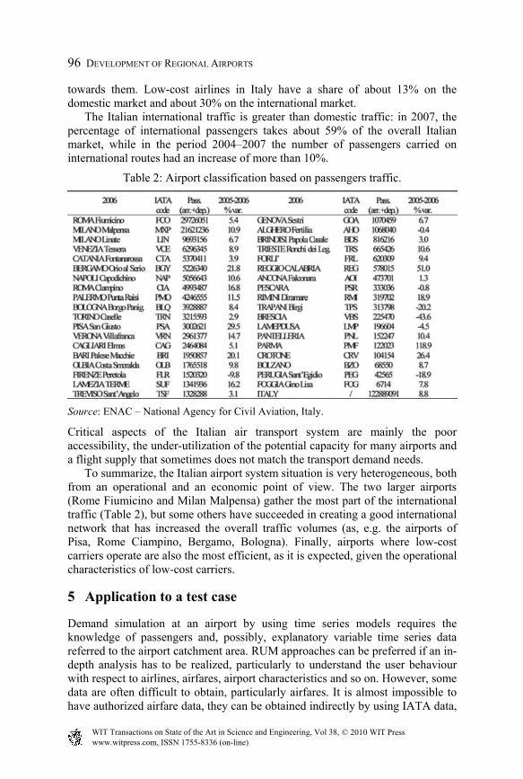
Following the EU classification, as shown in Table 2, in Italy there are 2 community airports (yearly passengers greater than 10 million), 5 national airports (yearly passengers from 5 to 10 million), 14 large regional airports (yearly passengers from 1 to 5 million) and 16 small regional airports (yearly passengers less than 1 million).
In recent years, the air demand in the Italian market has increased, following the general world tendency. According to forecasts provided by IATA and the European agency for the air transport safety (Eurocontrol), passenger volumes are expected to increase further in the future years; particularly, IATA [35, 36] predicts an average increase at a rate of about 3–4% starting from 2005, while Eurocontrol [37] predicts a yearly average increase in the European market at a rate of about 3% during the period 2005–2025. Anyway, short-medium trends are continuously revised due to contingent situations (as political stability, oil price and so on).
As for the Italian market, Eurocontrol forecasts a yearly average increase of about 2–3% for the domestic market, while international markets are expected to increase at a rate of about 4% for the next 8 years.
In the period 1997–2006, the annual passenger growth rate in the Italian market was about 6%; the Rome/Fiumicino-Milan/Linate pair has been the second busiest route within the EU market, with more than two million passengers carried (source: Eurostat, http://www.ec.europa.eu/eurostat). The analysis of the current situation in the Italian air market shows a rather scattered demand, probably due to the relatively high number of commercial airports per square mile; at the same time, the absence of an effective and widespread land network that can guarantee a suitable accessibility to/from the airport (mainly regional airports but also many national airports) reduces the potential air demand. Furthermore, in many cases the average distances among airports are about 130–160 kilometres, supplied air services are often similar and small airports are in competition to capture demand from overlapping catchment areas.
In this context, an important role is also played by airlines and their relationships with airports. Starting from the liberalization of the air transport system in Europe, more than 30 new commercial airlines have risen in Italy, but today less than half is still in the market and most of them have a marginal market share. Routes between many Southern Italy regional airports and the main airports (Rome, Milan above all) are operated by a few airlines without a significant competitiveness among them, while for some others airports, specially located in Northern Italy, supply exceeds demand.
Many regional airports offer point-to-point international links, often operated by low-cost companies; many of them serve tourist destinations in Northern Italy (as Venice, Florence) but seasonal flights at lower costs are also starting for more decentralized regions (as Sardinia, Calabria), thus improving the tourist flows
www.witpress.com, ISSN 1755-8336 (on-line) WIT Transactions on State of the Art in Science and Engineering, Vol 38, © 2010 WIT Press
96 DEVELOPMENT OF REGIONAL AIRPORTS towards them. Low-cost airlines in Italy have a share of about 13% on the domestic market and about 30% on the international market.
The Italian international traffic is greater than domestic traffic: in 2007, the percentage of international passengers takes about 59% of the overall Italian market, while in the period 2004–2007 the number of passengers carried on international routes had an increase of more than 10%.
Table 2: Airport classification based on passengers traffic.
Source: ENAC – National Agency for Civil Aviation, Italy.
Critical aspects of the Italian air transport system are mainly the poor accessibility, the under-utilization of the potential capacity for many airports and a flight supply that sometimes does not match the transport demand needs.
To summarize, the Italian airport system situation is very heterogeneous, both from an operational and an economic point of view. The two larger airports (Rome Fiumicino and Milan Malpensa) gather the most part of the international traffic (Table 2), but some others have succeeded in creating a good international network that has increased the overall traffic volumes (as, e.g. the airports of Pisa, Rome Ciampino, Bergamo, Bologna). Finally, airports where low-cost carriers operate are also the most efficient, as it is expected, given the operational characteristics of low-cost carriers.
5 Application to a test case
Demand simulation at an airport by using time series models requires the knowledge of passengers and, possibly, explanatory variable time series data referred to the airport catchment area. RUM approaches can be preferred if an in-depth analysis has to be realized, particularly to understand the user behaviour with respect to airlines, airfares, airport characteristics and so on. However, some data are often difficult to obtain, particularly airfares. It is almost impossible to have authorized airfare data, they can be obtained indirectly by using IATA data,
www.witpress.com, ISSN 1755-8336 (on-line) WIT Transactions on State of the Art in Science and Engineering, Vol 38, © 2010 WIT Press

AIR DEMAND MODELLING 97
but information on discounted airfare is very limited. Finally, the application of RUMs often requires passenger data collected by means of suitable surveys, while time series models can use general data easier to obtain (as population, GDP and so on).
In any case, to have information on the air demand at an airport, as a starting point to understand the airport general trend and without specific analyses on the user choice behaviour, time series models can represent a useful tool.
The application refers to the airport of Reggio Calabria, in the South of Italy (Figure 7), located very near the city centre (about 5 kilometres), well connected to the main road network but weakly served by public systems (both buses and trains). Thanks to its position in front of the island of Sicily and near the Aeolian isles, it might become an important node of the Mediterranean transport system, particularly with reference to leisure traffic flows.
Figure 7: Location of Reggio Calabria airport (Southern Italy) and its main competitive airport within the same administrative region.
The main competitive airport located in the same administrative region (Lamezia Terme) is about 140 kilometres far away. The second one, Catania Fontanarossa, is located in Sicily and the overall land distance is about 135 kilometres, but the access/egress time, included time spent to cross the Strait of Messina (between Sicily and Calabria), makes it less attractive to potential users.
As reported in Table 2, Lamezia Terme airport can be classified as a large regional airport and Catania as a national one, while Reggio Calabria is a small regional airport.
Starting from 2005, Reggio Calabria airport management has begun some developing policies by increasing the flight frequencies and the number of reached destinations. The new flights have been operated by some low-cost-like companies thus allowing lower fares for passengers. Before starting these
www.witpress.com, ISSN 1755-8336 (on-line) WIT Transactions on State of the Art in Science and Engineering, Vol 38, © 2010 WIT Press

98 DEVELOPMENT OF REGIONAL AIRPORTS developing policies, only hub-and-spoke flights were operated towards Rome and Milan by only two companies, one of them under a significant monopoly system. The new situation (more companies, more destinations both national and international, competition on some links) has had as consequence:
● the end of the monopoly system and then the opportunity to have more advantageous airfares;
● the opportunity to reach some destinations without transfer at hub(s); ● the increase of frequencies and the opportunity to choose among more
destinations and for the same destination among more departure times and airfares.
The current situation is still in a developing but uncertain stage. In fact, the presence of the competitive Lamezia Terme airport, that is continuously expanding its supply and the served demand, makes the growth of the airport difficult, given also that its role in terms of both kind of services and reached destinations (and then market share) is not well defined if compared with the competing airport.
Furthermore, the airport catchment area, obtained by means of some RP surveys at the airport, is rather limited from a geographical point of view (Figure 8), the most part being concentrated around the city of Reggio Calabria (about 52% of demand is resident in the municipality area) and its province (about 30%), while a little part comes from the city of Messina (Sicily). Finally, a negligible percentage comes from the nearest provinces of the Calabria administrative region.
During the years 2005 and 2006, three surveys were conducted at Reggio Calabria airport, within the research project ‘Methods and models to forecast the air passenger transport demand’, part of a more general national project entitled ‘Guidelines to plan the development of the Italian regional airports’. The goal of the surveys was to understand the main characteristics of users at the airports, to identify the catchment area and to have information on the airfare paid by users.
The first survey was realized immediately after the introduction of new links by new air companies, and the second one after some months during which more frequencies and more destinations were added. As Table 3 shows, the percentage of users in the price class 50–100 increases notably from the first to the second survey, while the percentage in the price class 0–50 is drastically reduced (really, this price class is linked to the initial launch bargain of new destinations with new companies). The increase of the percentage of users in the price class 50–100 is probably due to the presence of low-cost-like companies, that has had as an expected consequence the increase of competition on some routes and then a reduction of the average airfare.
The available, aggregate data refer to passengers and the main supply characteristics at the airports (as number of movements, frequencies, number of operating airlines and so on) for a given period (sources: Italian Official Statistic Institute ISTAT; Ministry of Infrastructure and Transport; Association of Italian Airports: www.assaeroporti.it).
www.witpress.com, ISSN 1755-8336 (on-line) WIT Transactions on State of the Art in Science and Engineering, Vol 38, © 2010 WIT Press

AIR DEMAND MODELLING 99
Figure 8: Catchment area of Reggio Calabria airport.
Table 3: Comparison between the 1st and 2nd survey: Price class.
Price class (Euro) Users [%] 1st survey Users [%] 2nd survey0–50 14.9 1.5 50–100 34.1 57.5 100–150 18.3 20.9 150–200 12.6 11.5 200–250 10.3 4.2 250–300 4.3 0.8 300–350 0.2 1.5 350–400 3.7 0.7 400–450 0.5 0.8 >450 1.1 0.5
Table 4 (and Figure 9) reports passengers data at the airport; note the outlier referred to 2004 when the airport was closed during the months of March, April and May for some adjustment work on the runway.
www.witpress.com, ISSN 1755-8336 (on-line) WIT Transactions on State of the Art in Science and Engineering, Vol 38, © 2010 WIT Press

100 DEVELOPMENT OF REGIONAL AIRPORTS Table 4: Boarded/de-planed passengers at the airport of Reggio Calabria (period
1989–2007)*.
Year Pax Year Pax Year Pax Year Pax 1989 157,225 1994 260,539 1999 543,041 2004 272,470 1990 245,711 1995 252,294 2000 538,048 2005 398,089 1991 222,571 1996 364,036 2001 481,857 2006 578,250 1992 246,306 1997 464,161 2002 463,662 2007 547,814 1993 266,782 1998 461,091 2003 441,795
* Data have been collected by using more sources, as a unique data base does not exist.
Figure 9: Passenger demand trend at the airport of Reggio Calabria (period 1989–2007).
After a positive trend from 1989 to 1999, the passenger demand has started to decrease systematically in successive years till 2004. The main reasons for this decrease are the progressive reduction of the supply and also the more and more expensive airfares. After 2004, the demand trend seems essentially positive, but the potential demand is probably higher even if a poor accessibility and the still uncertain developing policy at the airport stop its expansion. Starting from the same boarded/de-planned passenger data base, both univariate and multivariate time series models have been calibrated.
Following the Box-Jenkins approach, some preliminary analyses have been carried out; estimated ACF and PACF for the boarded/de-planned passenger time series (Figure 10) show that ACF decreases linearly and the value of PACF at lag 1 is close to 1, i.e. there is mean non-stationarity that has been removed by differencing the series once. After that transformation, the Dickey-Fuller test applied to the differenced series confirms its stationarity. To remove the variance non-stationarity, the series has been transformed by using the logarithmic function. The estimate of the partial autocorrelation coefficients shows that only π1 does not fall within the two standard error bounds ±2/√N (Figure 10), so the order 1 can be established for the AR component. The same procedure is applied to choose the MA component order by using the correlogram of ACF, that
www.witpress.com, ISSN 1755-8336 (on-line) WIT Transactions on State of the Art in Science and Engineering, Vol 38, © 2010 WIT Press
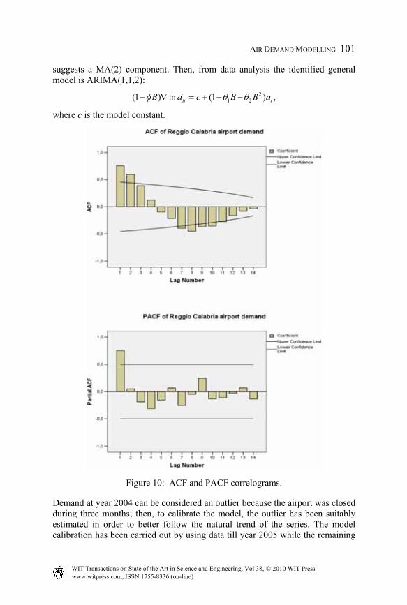
AIR DEMAND MODELLING 101
θ
suggests a MA(2) component. Then, from data analysis the identified general model is ARIMA(1,1,2):
21 2(1 ) ln (1 ) ,− ∇ = + − −it tB d c B B aφ θ
where c is the model constant.
Figure 10: ACF and PACF correlograms.
Demand at year 2004 can be considered an outlier because the airport was closed during three months; then, to calibrate the model, the outlier has been suitably estimated in order to better follow the natural trend of the series. The model calibration has been carried out by using data till year 2005 while the remaining
www.witpress.com, ISSN 1755-8336 (on-line) WIT Transactions on State of the Art in Science and Engineering, Vol 38, © 2010 WIT Press
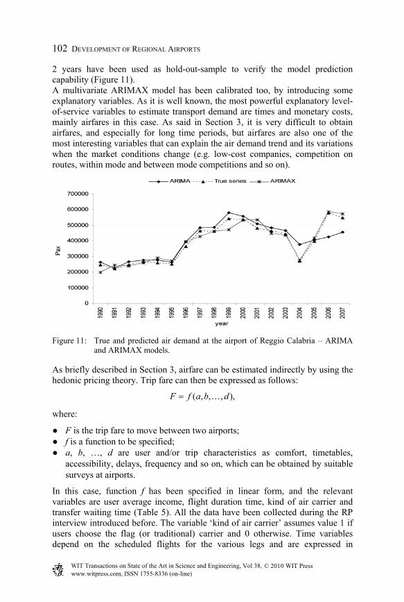
102 DEVELOPMENT OF REGIONAL AIRPORTS 2 years have been used as hold-out-sample to verify the model prediction capability (Figure 11). A multivariate ARIMAX model has been calibrated too, by introducing some explanatory variables. As it is well known, the most powerful explanatory level-of-service variables to estimate transport demand are times and monetary costs, mainly airfares in this case. As said in Section 3, it is very difficult to obtain airfares, and especially for long time periods, but airfares are also one of the most interesting variables that can explain the air demand trend and its variations when the market conditions change (e.g. low-cost companies, competition on routes, within mode and between mode competitions and so on).
Figure 11: True and predicted air demand at the airport of Reggio Calabria – ARIMA and ARIMAX models.
As briefly described in Section 3, airfare can be estimated indirectly by using the hedonic pricing theory. Trip fare can then be expressed as follows:
( , , , ),= …F f a b d
where:
● F is the trip fare to move between two airports; ● f is a function to be specified; ● a, b, …, d are user and/or trip characteristics as comfort, timetables,
accessibility, delays, frequency and so on, which can be obtained by suitable surveys at airports.
In this case, function f has been specified in linear form, and the relevant variables are user average income, flight duration time, kind of air carrier and transfer waiting time (Table 5). All the data have been collected during the RP interview introduced before. The variable ‘kind of air carrier’ assumes value 1 if users choose the flag (or traditional) carrier and 0 otherwise. Time variables depend on the scheduled flights for the various legs and are expressed in
www.witpress.com, ISSN 1755-8336 (on-line) WIT Transactions on State of the Art in Science and Engineering, Vol 38, © 2010 WIT Press

AIR DEMAND MODELLING 103
hours. Finally, fares, transformed by using the logarithmic function, refer to one-way trips.
Table 5: Results of the fare model.
Variable Coefficients t-student (1%) Income 0.88 23.93 Flight duration 1.45 26.88 Kind of airline 0.47 6.43 Waiting time –0.82 –13.39 Statistical tests R2 Adjusted R2 0.958 0.9579
As Table 5 shows, all the parameters have correct signs and are statistically significant as well as the overall model (see R2 and adjusted R2). Users are willing to pay more for longer trips, but prefer direct flights or good connections, as the negative value of the waiting time variable suggests. Furthermore, despite a greater monetary cost they prefer flag carriers, probably due to the image of reliability and safety they inspire.
Generally, after the calibration of a fare model, its results can be used into a demand model as ARIMAX. In any case, even if this fare model specification has given good results in terms of descriptive power, for this application not all the time series data of the explanatory variables are available and then the fare model results cannot be used into an ARIMAX model. Then the explanatory variables considered here are the number of movements at the airport at year t, mt, and the average per capita income at year t, It, that can be considered a proxy of the willingness to pay, and in some ways linked to the airfares at the airport. The number of movements is a level-of-service variable, representing the capability of the airport to offer flights, while income is a socio-economic variable depending on the activity system in the catchment area.
The sequential testing procedure described in Section 3.1 allows the P values for both variables to be identified; particularly, demand at year t depends on movements in the same year t and income from year t to year t–6. The resulting multivariate ARIMAX model is:
21 2 1 2 1
3 2 4 3 5 4 6 5 7 6
(1 ) ln (1 ) ln ln lnln ln ln ln ln .
−
− − − − −
−Φ ∇ = − − ⋅ + ⋅ + + ++ + + + + +
t t t t
t t t t t
B d B B a m I II I I I I
θ θ δ α αα α α α α κ
t
The model has been calibrated by using data from 1989 to 2005, while the remaining data (2006–2007) were used as hold-out sample (Figure 11). As Figure 11 shows, both ARIMA and ARIMAX models can well predict the air demand at the airport; years from 2005 to 2007, considered as hold-out sample, are better simulated by the ARIMAX model. Anyway, it is interesting to note that both models show good performances, although the theoretically most appealing multivariate model needs more explanatory variables to capture the
www.witpress.com, ISSN 1755-8336 (on-line) WIT Transactions on State of the Art in Science and Engineering, Vol 38, © 2010 WIT Press

104 DEVELOPMENT OF REGIONAL AIRPORTS demand trend. In some cases, the ARIMA model explains the demand trend better than the ARIMAX model. However, apart from the similar simulation capabilities, multivariate models can help to test possible developing policies by means of suitable hypotheses about the values of the explanatory variables. In this case, the level-of-service explanatory variable (movements) depends on the airport management and airline policies, while income depends on socio-economic developing policies, more complex and more difficult to estimate and control. Without specific developing policies on the territory and then all things being equal, income follows its trend, while hypotheses can be made on the number of movements in order to verify if and how demand can further increase.
number of movements
0
2000
4000
6000
8000
10000
1989
1990
1991
1992
1993
1994
1995
1996
1997
1998
1999
2000
2001
2002
2003
2004
2005
2006
2007
Figure 12: Number of movements trend at the airport of Reggio Calabria (period
1989–2007).
It is interesting to compare the trend of the number of movements (Figure 12) and passenger demand percentage variations at the airport (Figure 13) as well as the percentage variations with respect to 1999 (corresponding to the greatest demand value before 2005, when new companies began to operate at the airport). From Figure 13, it can be seen that the percentage variations of movements and passengers are rather similar, apart from the transition year 2005, when many developing policies started at the airport. More interestingly, Figure 14 shows the percentage variations with respect to the reference year 1999. In this case, till 2004 demand is decreasing quicker than the number of movements with respect to the reference year, but at a rather similar rate. After 2005, while the number of movements increases strongly, demand increases weakly and simply reaches the values already achieved at 1999.
The analyses of data thus suggest that the policies started at the airport do not capture the actual needs of passengers, as demand at years 2006–2007, practically equal to demand at year 1999, is satisfied by a supply really larger than that at the reference year. Then, even if the number of movements increases – suggesting more possible destinations, greater frequencies for the same destination, more flights at different times of the day – demand does not increase significantly with respect to the reference year 1999, when the number of movements was largely lower, but probably more suitable for the passengers needs.
www.witpress.com, ISSN 1755-8336 (on-line) WIT Transactions on State of the Art in Science and Engineering, Vol 38, © 2010 WIT Press

AIR DEMAND MODELLING 105
-60,0
-40,0-20,0
0,0
20,0
40,060,0
80,0
% pax variation % mov variation
% pax variation 17,8 -0,9 -10,4 -3,8 -4,7 -38,3 46,1 45,3 -5,3
% mov variation 13,8 -0,1 -2,1 -5,3 -4,5 -39,2 69,5 58,4 -5,1
1999 2000 2001 2002 2003 2004 2005 2006 2007
Figure 13: Number of movements and passenger demand percentage variations at the airport of Reggio Calabria.
Figure 14: Number of movements and passenger demand percentage variations at the airport of Reggio Calabria with respect to year 1999.
To simulate the relationship between demand needs and air supply, probably the time series model should use more level-of-service explanatory variables taking into account not only the amount of supply but its distribution and its specific characteristics. However, when the required level-of-detail increases, data are more difficult to obtain, as official agencies at national and international level (as Eurostat) generally provide considerably aggregate data. Then, specific surveys have to be carried out that also allow combined time series and RUM to be used.
As the application at the regional airport of Reggio Calabria has showed, the regular collection of data at a given airport can be of great importance for the airport management, helping them to identify the best developing strategies, particularly when competition between airports exists. In this case, the decrease in demand despite the increase in the flight number can be due to the superior
www.witpress.com, ISSN 1755-8336 (on-line) WIT Transactions on State of the Art in Science and Engineering, Vol 38, © 2010 WIT Press

106 DEVELOPMENT OF REGIONAL AIRPORTS supply at the nearest competing airport, that in fact has strongly increased its demand, probably becoming attractive for people initially being in the Reggio Calabria airport catchment area.
From a modelling point of view, the results obtained with both univariate and multivariate time series models do not allow asserting that univariate models are better than multivariate models and vice versa. As obtained in this study, the better forecasting power of the univariate model is offset by its limits of validity, which depends on the stability of the boundary conditions. Multivariate models solve this problem by using explanatory variables, whose time series, however, are often difficult to find. Thus, the potential explanatory power of multivariate time series models is limited by the lack of suitable data.
References
[1] Graham, B. & Guyer, C., Environmental sustainability, airport capacity and European air transport liberalization: Irreconcilable goals? Journal of Transport Geography, 7(3), pp. 165–180, 1999.
[2] Cohas, F., Belobaba, P. & Simpson, R., Competitive fare and frequency effects in airport market share modelling. Journal of Air Transport Management, 2(1), pp. 33–45, 1995.
[3] Air Transport Action Group (ATAG), The economic & social benefits of air transport, September 2005, www.atag.org.
[4] Italian Ministry of Transport, National Transport Analysis, Rome: Istituto Poligrafico di Stato, 1998.
[5] Transport Canada, Regional and Small Airports Study (TP 14283B), 2004. [6] Harvey, G., Airport Choice in a Multiple Airport Region. Transportation
Research, 21A(6), pp. 439–449, 1987. [7] Ashford, N. & Benchemam, M., Passengers’ choice of airport: An
application of the multinomial logit model. Transportation Research Record, 1147, pp. 1–5, 1987.
[8] Hess, S. & Polak, J.W., Mixed logit modelling of airport choice in multi-airport regions. Journal of Air Transport Management, 11(2), pp. 59–68, 2005.
[9] Fuellhart, K., Airport catchment and leakage in a multi-airport region: The case of Harrisburg International. Journal of Transport Geography, 15(4), pp. 231–244, 2007.
[10] Van Reeven, P., de Vlieger, J. & Karamychev, V., BOB airport accessibility pilot, final report within the Fifth Framework Program for research, technological development, Erasmus University Rotterdam, Transport Economics Dept, 2003.
[11] Milone, R., Humeida, H., Moran, M., Seifu, M. & Hogan, J., FY-2003 Models development program for COG/TPB travel models, Metropolitan Washington Council of Governments, National Capital Region Transportation Planning Board, 2003.
www.witpress.com, ISSN 1755-8336 (on-line) WIT Transactions on State of the Art in Science and Engineering, Vol 38, © 2010 WIT Press

AIR DEMAND MODELLING 107
[12] Suzuki, Y., Modelling and testing the ‘two-step’ decision process of
travellers in airport and airline choices. Transportation Research, 43E(1), pp. 1–20, 2007.
[13] Button, K., The European market for airlines transportation and multimodalism, Airports as multimodal interchange nodes, Economic Research Centre, European Conference of Ministers of Transport 2005, http://internationaltransportforum.org/europe/ecmt/pubpdf/05RT126.pdf.
[14] Cascetta, E., Transportation Systems Engineering: Theory and Methods, Kluwer: The Netherlands, 2001.
[15] Ben Akiva, M. & Lerman, S., Discrete Choice Analysis, Cambridge, MA: MIT Press, 1985.
[16] Rosen, S., Hedonic prices and implicit market: Product differentiation in pure competition. Journal of Political Economy, 82, pp. 34–55, 1974.
[17] Hensher, D.A., Determining passenger potential for a regional airline hub at Canberra International Airport. Journal of Air Transport Management, 8(5), pp. 301–311, 2002.
[18] Andreoni, A. & Postorino, M.N., A multivariate ARIMA model to forecast air transport demand. Proc. of the European Transport Conference 2006, www.aetransport.org.
[19] Inglada, V. & Rey, B., Spanish air travel and September 11 terrorist attacks: A note. Journal of Air Transport Management, 10(6), pp. 441–443, 2004.
[20] Karlaftis, M.G. & Papastavrou, J.D., Demand characteristics for charter air-travel. International Journal of Transport Economics, XXV(3), pp. 19–35, 1998.
[21] Lim, C. & McAleer, M., Time series forecasts of international travel demand for Australia. Tourism Management, 23(4), pp. 389–396, 2002.
[22] Lai, L. & Lu, L., Impact analysis of September 11 on air travel demand in the USA. Journal of Air Transport Management, 11(6), pp. 455–458, 2005.
[23] Melville, J.A., An empirical model of the demand for international air travel for the Caribbean region. International Journal of Transport Economics, XXV(3), pp. 313–336, 1998.
[24] Box, G.E.P. & Jenkins, G.M., Time-Series Analysis, Forecasting and Control, San Francisco: Holden-Day, 1970.
[25] Judge, G.G., Introduction to the Theory and Practice of Econometrics, 2nd edition, New York: Wiley & Sons, 1988.
[26] Makridakis, S., Wheelwright, S.C. & Hyndman R.J., Forecasting. Methods and Applications, 3rd edition, New York: Wiley & Sons, 1998.
[27] Ljung, M.G. & Box, G.E.P., On a measure of lack of fit in time series model. Biometrika, 65, pp. 297–303, 1978.
[28] Jarque, C.M. & Bera, A.K., Model specification tests: A simultaneous approach. Journal of Econometrics, 20(1, A), pp. 59–82, 1982.
[29] Bhat, C.R., A heteroscedastic extreme value model of intercity travel mode choice. Transportation Research, 29B(6), pp. 471–483, 1997.
[30] Bhat, C.R., Covariance heterogeneity in nested logit models: Econometric structure and application to intercity travel. Transportation Research, 31B(1), pp. 11–21, 1997.
www.witpress.com, ISSN 1755-8336 (on-line) WIT Transactions on State of the Art in Science and Engineering, Vol 38, © 2010 WIT Press
108 DEVELOPMENT OF REGIONAL AIRPORTS [31] Kroes, E., Lierens, A. & Kouwenhoven, M., The airport network and
catchment area competition model: A comprehensive airport demand forecasting system using a partially observed database. Proceedings of ERSA 2005.
[32] Postorino, M.N. & Versaci, M., A neuro-fuzzy approach to simulate the user mode choice behaviour in a travel decision framework. International Journal of Modelling and Simulation, 27(4), 2007.
[33] Sadek, A.W., Spring, G. & Smith, B.L., Towards more effective transportation applications of computational intelligence paradigms. Transportation Research Record, 1836, pp. 57–63, 2003.
[34] Pribyl, O. & Goulias K.G., Application of adaptive neuro-fuzzy inference system to analysis of travel behaviour. Transportation Research Record, 1854, pp. 180–188, 2003.
[35] IATA, Air/rail intermodality study, Brussels, 2003. [36] IATA, Passenger and freight forecast publications 2005–2009,
www.iata.org. [37] Eurocontrol, STATFOR, Long-term forecast of air traffic (1006–2025)
report, www.eurocontrol.int/statfor, 2003.
www.witpress.com, ISSN 1755-8336 (on-line) WIT Transactions on State of the Art in Science and Engineering, Vol 38, © 2010 WIT Press