3D Elastic Full Waveform Inversion - On Land Study case
5
30 May – 2 June 2016 | Reed Messe Wien 78 th EAGE Conference & Exhibition 2016 Vienna, Austria, 30 May – 2 June 2016 Tu SRS2 08 3D Elastic Full Waveform Inversion - On Land Study case J.A. Kormann* (Barcelona Supercomputing Center), D. Marti (Institute of Earth Sciences Jaume Almera), J.E. Rodriguez (Barcelona Supercomputing Center), I. Marzan (Institute of Earth Sciences Jaume Almera), N. Gutierrez (Barcelona Supercomputing Center), M. Ferrer (Barcelona Supercomputing Center), M. Hanzich (Barcelona Supercomputing Center), J. de la Puente (Barcelona Supercomputing Center), R. Carbonell (Institute of Earth Sciences Jaume Almera), J.M. Cela (Barcelona Supercomputing Center) & S. Fernandez (REPSOL) SUMMARY Full Waveform Inversion is one of the most advanced processing methods that is recently reaching a mature state after years of solving theoretical and technical issues such as the non-uniqueness of the solution and harnessing the huge computational power required by realistic scenarios. In this work, we present the application of this method to a 3D on-land dataset acquired to characterize the shallow subsurface. The current study explores the possibility to apply elastic isotropic Full Waveform Inversion using only the vertical component of the recorded seismograms. One of the main challenges in this case study remains the costly 3D modeling that includes topography and free surface effects. Nevertheless, the resulting models provide a higher resolution of the subsurface structures than starting models, and show a good correlation with the available borehole measurements.
Transcript of 3D Elastic Full Waveform Inversion - On Land Study case

30 May – 2 June 2016 | Reed Messe Wien
78th EAGE Conference & Exhibition 2016 Vienna, Austria, 30 May – 2 June 2016
Tu SRS2 083D Elastic Full Waveform Inversion - On LandStudy caseJ.A. Kormann* (Barcelona Supercomputing Center), D. Marti (Institute ofEarth Sciences Jaume Almera), J.E. Rodriguez (Barcelona SupercomputingCenter), I. Marzan (Institute of Earth Sciences Jaume Almera), N. Gutierrez(Barcelona Supercomputing Center), M. Ferrer (BarcelonaSupercomputing Center), M. Hanzich (Barcelona Supercomputing Center),J. de la Puente (Barcelona Supercomputing Center), R. Carbonell (Instituteof Earth Sciences Jaume Almera), J.M. Cela (Barcelona SupercomputingCenter) & S. Fernandez (REPSOL)
SUMMARYFull Waveform Inversion is one of the most advanced processing methods that is recently reaching amature state after years of solving theoretical and technical issues such as the non-uniqueness of thesolution and harnessing the huge computational power required by realistic scenarios. In this work, wepresent the application of this method to a 3D on-land dataset acquired to characterize the shallowsubsurface. The current study explores the possibility to apply elastic isotropic Full Waveform Inversionusing only the vertical component of the recorded seismograms. One of the main challenges in this casestudy remains the costly 3D modeling that includes topography and free surface effects. Nevertheless, theresulting models provide a higher resolution of the subsurface structures than starting models, and show agood correlation with the available borehole measurements.

30 May – 2 June 2016 | Reed Messe Wien
78th EAGE Conference & Exhibition 2016 Vienna, Austria, 30 May – 2 June 2016
Introduction
In this work we present the application of isotropic Elastic Full Waveform Inversion (E-FWI) to a realdataset. The studied area is located within the Loranca Basin (Spain) and presents a smooth topographywhich is part of the challenge propose here. In order to characterize the very shallow surface, a 3Dseismic data volume was acquired in a square area of 540x540 m2. Although originally designed toperform a high resolution Travel-Time Tomography (TTT), we take advantage of the data to performFWI. We propose to perform E-FWI because the target structures are close to the surface (< 120 mdeep) making wave propagation to be mostly driven by elastic effects. On the other hand, it potentiallycan be more resolutive than its acoustic counterpart providing clear imaging improvements in somescenarios (Vigh et al., 2014; Raknes et al., 2015).
This dataset is part of an ongoing multidisciplinary geophysical, geological, hydrological characteriza-tion of an area which has been proposed as a possible site to host a temporal radioactive waste disposalsite. Therefore, a large amount of multidisciplinary data revealing information on the underground isavailable including down-hole and other geophysical measurements.
In our scenario, we include free-surface effects, and consequently take topography into account. We willshow that the resulting models provide a better understanding of the geological features of the area andas well as a good correlation with borehole measurements.
Theory
On one hand, we use the time-domain elastic isotropic approach for solving the elastic wave equationby means of a Fully staggered grid combined with mimetic operators (de la Puente et al., 2014)
ρ(x)v̇(x, t) = ∇ ·σ(x, t)+ fs(xs, t),
σ̇(x, t) = C(x) : ∇v(x, t)(1)
where fs is the source function at positionxs, v the particle velocity,ρ the density (set as a constant), andσ the stress field. ths gris is deformed to accomodate the local topography.
On the other hand, the mathematical formulation of FWI consists in the minimization of a error functionE(m,mreal) (Pratt, 1999; Virieux and Operto, 2009), wherem andmreal are the current and target modelrespectively. In this study we employ the normalized least-square criterionL2 given by
Ek(mk,m real ) =
12
N∑
i=1
n∑
j=1
uij(xr,xs;mk)
maxj
(|ui(xr,xs;mk )|)−
uij(xr,xs;mreal)
maxj
(|ui(xr,xs;mreal)|)
2
,(2)
whereN is the number of receivers,n the number of samples of each trace,xr andxs are the receiver andsource position respectively,u(xr,xs;mk) andu(xr,xs;mreal) stand for the displacement obtained usingthe current model parameters at thekth iteration and the experimental dataset respectively.
Our approach for E-FWI consists in constraining the maximum offset to the longest wavelength at thecurrent frequency in a multi-scale approach. We call this approach Dynamic Offset Control (DOC).It aims to use smaller offset for reflection data when increasing frequency. Thus, we select the offsetaccording to
O f f set = V/ f0 (3)
where f0 is the cut-off frequency of the low-pass filter applied to the data and V a parameter to be definedby the user. This strategy has the side effect of reducing the computational domain as we go into higherfrequencies while minimizing the effect of the surface waves on the gradients. We emprically found thatV equal to max(Vp) shows to be a sufficient condition. We want to stress that the computational grid
30 May – 2 June 2016 | Reed Messe Wien
78th EAGE Conference & Exhibition 2016 Vienna, Austria, 30 May – 2 June 2016
is adapted to the shortest wavelength present in the models anddoes not match the receiver and sourcegrids. Besides, no part of the model has been fixed.
We apply gradient preconditioning in two steps: first we invert forlog(m) instead ofm, and secondlywe compensate for spreading by using the square of the illumination. In all our tests, it shows to be anefficient preconditioning.
(a)
Tim
e (s
)
FWI shotgather
50 100 150 200 250 300 350 400 450
0
0.05
0.1
0.15
0.2
0.25
Tim
e (s
)
Receiver
Orignal shot gather
50 100 150 200 250 300 350 400 450
0.05
0.1
0.15
0.2
(b)
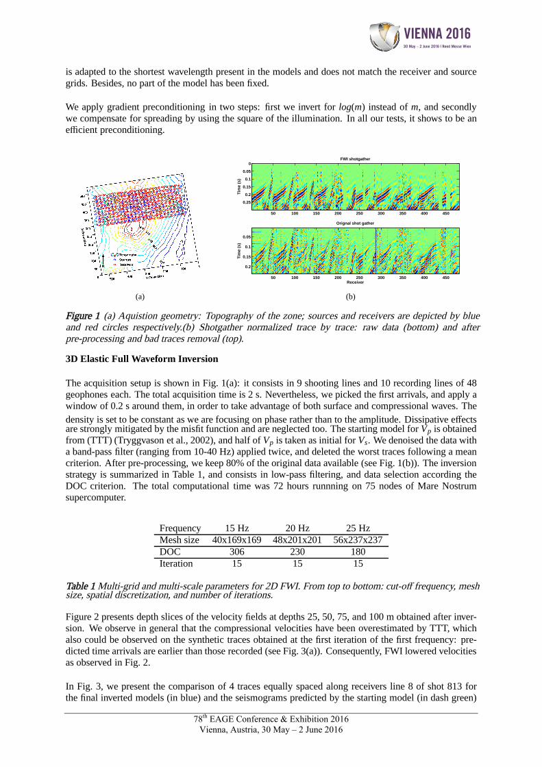
Figure 1 (a) Aquistion geometry: Topography of the zone; sources and receivers are depicted by blue and red circles respectively.(b) Shotgather normalized trace by trace: raw data (bottom) and after pre-processing and bad traces removal (top).
3D Elastic Full Waveform Inversion
The acquisition setup is shown in Fig. 1(a): it consists in 9 shooting lines and 10 recording lines of 48 geophones each. The total acquisition time is 2 s. Nevertheless, we picked the first arrivals, and apply a window of 0.2 s around them, in order to take advantage of both surface and compressional waves. The density is set to be constant as we are focusing on phase rather than to the amplitude. Dissipative effects are strongly mitigated by the misfit function and are neglected too. The starting model for Vp is obtained from (TTT) (Tryggvason et al., 2002), and half of Vp is taken as initial for Vs. We denoised the data with a band-pass filter (ranging from 10-40 Hz) applied twice, and deleted the worst traces following a mean criterion. After pre-processing, we keep 80% of the original data available (see Fig. 1(b)). The inversion strategy is summarized in Table 1, and consists in low-pass filtering, and data selection according the DOC criterion. The total computational time was 72 hours runnning on 75 nodes of Mare Nostrum supercomputer.
Frequency 15 Hz 20 Hz 25 HzMesh size 40x169x169 48x201x201 56x237x237DOC 306 230 180Iteration 15 15 15
Table 1 Multi-grid and multi-scale parameters for 2D FWI. From top to bottom: cut-off frequency, mesh size, spatial discretization, and number of iterations.
Figure 2 presents depth slices of the velocity fields at depths 25, 50, 75, and 100 m obtained after inver-sion. We observe in general that the compressional velocities have been overestimated by TTT, which also could be observed on the synthetic traces obtained at the first iteration of the first frequency: pre-dicted time arrivals are earlier than those recorded (see Fig. 3(a)). Consequently, FWI lowered velocities as observed in Fig. 2.
In Fig. 3, we present the comparison of 4 traces equally spaced along receivers line 8 of shot 813 for the final inverted models (in blue) and the seismograms predicted by the starting model (in dash green)

30 May – 2 June 2016 | Reed Messe Wien
78th EAGE Conference & Exhibition 2016 Vienna, Austria, 30 May – 2 June 2016
at frequency 25 Hz. We observe that the velocity models allow topredict much better the travel timesof the recorded data. Finally, fittings of the borehole SVC6 with velocity depth profiles (located nearthe borehole but not at the exact position) have also been improved respect to those from the startingmodels: we observed a good agreement of the low-frequency content for bothVs andVp (see Fig. 3).
X−d
irect
ion
0 200 400
0
200
4001000
2000
3000
4000
X−d
irect
ion
0 200 400
0
200
4002000
3000
4000
X−d
irect
ion
0 200 400
0
200
4002000
2500
3000
3500
4000
Y−Direction
X−d
irect
ion
0 200 400
0
200
400
2500
3000
3500
4000
4500
0 200 400
0
200
4001000
2000
3000
4000
0 200 400
0
200
4002000
3000
4000
0 200 400
0
200
4002000
2500
3000
3500
4000
Y−Direction0 200 400
0
200
400
2500
3000
3500
4000
4500
0 200 400
0
200
400500
1000
1500
2000
0 200 400
0
200
4001000
1500
2000
0 200 400
0
200
4001000
1500
2000
Y−Direction0 200 400
0
200
400
1200140016001800200022002400
Figure 2 Four detph slices for Vp and Vs velocities. From left to right: Vp starting model, inverted Vp, and inverted Vs. From top to bottom: depth 25, 50, 75, and 100 m.
Conclusions
We have presented a 3D Elastic FWI successfully working on land real data including topography, using only near-source offsets. For this purpose, we have introduced an offset selection method called Dynamic Offset Control. This technique allows us to reduce the maximum aperture of each shot in FWI, hence reducing the computational cost when moving into higher frequencies, a key point for elastic inverison. E-FWI clearly improves our knowledge of the shallow subsurface structures, as observed when comparing inverted models with the borehole measurements.
Acknowledgements
The authors thank Repsol for the permission to publish the present research and for funding through the Aurora project. J. Kormann also thankfully acknowledges the Spanish Supercomputing Network (RES) through grant FI-2014-2-0009. Funding support for the data acquisition and access to the available geophysical data was provided by ENRESA. The GFZ Instrument Pool provided the instrumentation for the data acquisition. This project was partially funded by the European Union’s Horizon 2020 research and innovation programme under the Marie Sklodowska-Curie grant agreement No 644602.

30 May – 2 June 2016 | Reed Messe Wien
78th EAGE Conference & Exhibition 2016 Vienna, Austria, 30 May – 2 June 2016
0 0.05 0.1 0.15 0.2 0.25 0.3 0.35 0.4
−1
0
1
Nor
mal
ized
A
mpl
itude
0 0.05 0.1 0.15 0.2 0.25 0.3 0.35 0.4
−1
0
1
Nor
mal
ized
A
mpl
itude
0 0.05 0.1 0.15 0.2 0.25 0.3 0.35 0.4
−1
0
1
Nor
mal
ized
A
mpl
itude
0 0.05 0.1 0.15 0.2 0.25 0.3 0.35 0.4
−1
0
1
Nor
mal
ized
A
mpl
itude
Time (s)(a)
0 50 100
500
1000
1500
2000
2500
Vs
Vs (
m/s
)
0 50 1001000
1500
2000
2500
3000
3500
4000
4500
Vp (
m/s
)
Depth (m)(b)
Vp
SCV6
FWI
Starting
SCV6
FWI
Starting
Data
Starting
FWI
Figure 3 (a) Shot 813 (line8, position 13): Comparison between traces from the target, starting and inverted models(red, green and blue lines respectively) for 4 receivers equally spaced along recording line. (b) Comparison with measurement from SVC6: Vs (top) and Vp (bottom).
References
Pratt, R.G. [1999] Seismic waveform inversion in the frequency domain, Part 1: Theory and verification in a physical scale model. Geophysics, 64, 888-901.
de la Puente, J., Ferrer, M., Hanzich, M., Castillo, J.E. and Cela, J.M. [2014] Mimetic seismic wave modeling including topography on deformed staggered grids. Geophysics, 79(3), T125-T141.
Raknes, E.B., Arntsen, B. and Weibull, W. [2015] Three-dimensional elastic full waveform inversionusing seismic data from the Sleipner area. Geophysical Journal International, 202, 1877-1894.
Tryggvason, A., Rögnvaldsson, S. and Flovenz, Ó.G.. [2002] Three-dimensional imaging of P- and S-wave velocity structure and earthquake locations beneath southwest Iceland. Geophysical Journal International, 171(5), 848-866.
Vigh, D., Jiao, K., Watts, D. and Sun, D. [2014] Elastic full-waveform inversion application using multicomponent measurements of seismic data collection. Geophysics, 79(2), R63-R77.
Virieux, J. and Operto, S. [2009] An overview of full-waveform inversion in explorat ion geophysics. Geophysics, 74, WCC127-WCC152.