
3D Computer Vision - - TU Kaiserslautern · Triangulation Drift reduction ... Code, videos, papers,...
53
1 Structure from motion II Prof. Didier Stricker Dr. Gabriele Bleser Kaiserlautern University http://ags.cs.uni-kl.de/ DFKI – Deutsches Forschungszentrum für Künstliche Intelligenz http://av.dfki.de 3D Computer Vision
Transcript of 3D Computer Vision - - TU Kaiserslautern · Triangulation Drift reduction ... Code, videos, papers,...

1
Structure from motion II
Prof. Didier Stricker
Dr. Gabriele Bleser
Kaiserlautern University
http://ags.cs.uni-kl.de/
DFKI – Deutsches Forschungszentrum für Künstliche Intelligenz
http://av.dfki.de
3D Computer Vision
2
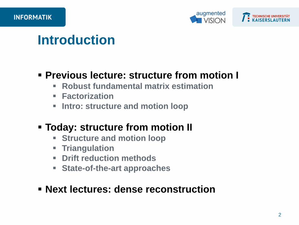
Previous lecture: structure from motion I Robust fundamental matrix estimation
Factorization
Intro: structure and motion loop
Today: structure from motion II Structure and motion loop
Triangulation
Drift reduction methods
State-of-the-art approaches
Next lectures: dense reconstruction
Introduction

3
Recall: structure and motion (SAM)
Reconstruct
Sparse scene geometry
Camera motion
Unknown
camera
viewpoints

4
Reminder: coordinate systems
[W]orld
mw
Rcw
Homogenization =
division through zc
mc
𝑤𝑐
5
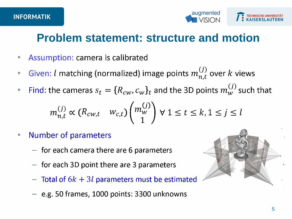
Problem statement: structure and motion

6
Offline:
E.g. as basis for dense 3D model
reconstruction
No real-time requirements, all
images are available at once
Offline vs. online structure and motion Online:
• E.g. for mobile Augmented Reality
in unknown environments
• Real-time requirements, images
become available one by one,
output required at each time-step

7
Offline:
Use MANY features and
computationally intense image
processing methods
Forward and backward feature
matching
Batch processing, e.g. bundle
adjustment
Offline vs. online structure and motion
Online:
• Reduced number of features
and lightweight image
processing methods
• Sequential/recursive
processing scheme
• Possibly local bundle
adjustment (keyframe/window
based)
harder problem

8
Online structure and motion (basic pipeline)
Image processing Camera
image
Scene model
Pose estimation Point
correspondences
Structure estimation
Additional sensor information?
Camera
pose

9
Alternating estimation of camera poses and 3D
feature locations (triangulation) from a (continuous)
image sequence.
Online structure and motion (calibrated case)
Camera pose
2D feature location
(from image processing)
How do we initialize the first camera poses?
𝑡 = 1
𝑡 = 2

10
Compute the fundamental matrix, 𝐹, from point
correspondences
Compute the camera poses from the fundamental matrix by
factorization:
Recall: 𝐹 = 𝐾′−𝑇 𝑡 ×𝑅𝐾−1
Obtain: 𝑃 = 𝐾 𝐼 0 , 𝑃′ = 𝐾′ 𝑅 𝑡
Note: 𝐾 and 𝐾′ are the intrinsic camera parameters
𝑃 and 𝑃′ are the projection matrices of both cameras
𝑅 and 𝑡 are the relative rotation and translation between both
cameras
Reminder: F-matrix estimation
𝑥 𝑥′
𝑋
𝑃 𝑃′
𝐹

0)]([ xRtx RtExExT ][with0
X
x x’
The vectors x, t, and Rx’ are coplanar
Essential Matrix
(Longuet-Higgins, 1981)
Epipolar constraint: calibrated case
11

Given: n corresponding points
compute the fundamental matrix F
such that
Solution
Problem statement
12

The “8-point” algorithm – Least squares solution
See lecture on parameter estimation! 13

Decomposing the fundamental matrix
Form the Essential matrix
See previous lecture
14

The 3D point is only in front of both cameras in one case
The four camera solutions
15

Alternating estimation of camera poses and 3D
feature locations (triangulation) from a (continuous)
image sequence.
Online structure and motion (calibrated case)
Camera pose
2D feature location
(from image
processing)
Now we have the two first camera poses.
How do we go on?
𝑡 = 1
𝑡 = 2
16

17
Alternating estimation of camera poses and 3D
feature locations (triangulation) from a (continuous)
image sequence.
Online structure and motion (calibrated case)
Camera pose
2D feature location
(from image
processing)
3D feature
location
Triangulate 3D points
𝑡 = 1
𝑡 = 2

18
Alternating estimation of camera poses and 3D
feature locations (triangulation) from a (continuous)
image sequence.
Online structure and motion (calibrated case)
Camera pose
2D feature location
(from image
processing)
3D feature
location
Estimate next camera
pose (now from 2D/3D
correspondences)
𝑡 = 1
𝑡 = 2 𝑡 = 3

19
Alternating estimation of camera poses and 3D feature
locations (triangulation) from a (continuous) image
sequence.
Online structure and motion (calibrated case)
Camera pose
2D feature location
(from image
processing)
3D feature
location
Triangulate additional
3D points
𝑡 = 1
𝑡 = 2 𝑡 = 3

20
Alternating estimation of camera poses and 3D
feature locations (triangulation) from a (continuous)
image sequence.
Online structure and motion (calibrated case)
Camera pose
2D feature location
(from image
processing)
3D feature
location
Refine known 3D points
with new camera poses
𝑡 = 1
𝑡 = 2 𝑡 = 3

21
Alternating estimation of camera poses and 3D feature
locations (triangulation) from a (continuous) image
sequence.
Online structure and motion (calibrated case)
Camera pose
2D feature location
(from image
processing)
3D feature
location
Refine known cameras
with new 3D points
E.g. for some selected
keyframes or more
extensively in offline SAM
𝑡 = 1
𝑡 = 2 𝑡 = 3

22
Drift: accumulating error
Structure and motion: the big problem
23
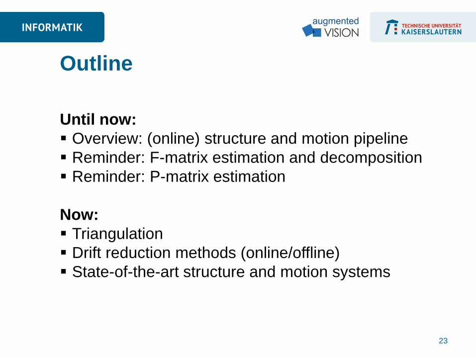
Until now:
Overview: (online) structure and motion pipeline
Reminder: F-matrix estimation and decomposition
Reminder: P-matrix estimation
Now:
Triangulation
Drift reduction methods (online/offline)
State-of-the-art structure and motion systems
Outline
Triangulation
24

25
Estimate the 3D point, 𝑋, given at least 2 known cameras, 𝐶
and 𝐶′, and 2 corresponding feature points, 𝑥 and 𝑥′, (i.e. 2
camera views).
• Hartley R. and Sturm P.: Triangulation, International Conference
on Computer Analysis of Images and Patterns, 1995.
Triangulation
𝑥 x’
𝑋
C C’

Then, 𝑦 = 𝑦′ and depth 𝑍 can be
computed from disparity:
Derivation via equal triangles
Note: feature displacement (disparity) is inversely
proportional to depth
26
Parallel cameras (simple case)
x
x’ d
Z
as 𝑑 → 0, 𝑍 → ∞

27
Arbitrary camera poses 3D triangulation required
General configuration
x1j
x2j
x3j
Xj
C1
C2
C3

Given: corresponding measured (i.e. noisy) feature points., and and
camera poses, and
Problem: in the presence of noise, back projected rays do not intersect
and measured points do not lie on corresponding epipolar lines
Triangulation
Rays are skew in space
How could this be solved?
28

29
Compute the mid-point of the shortest line between the
two rays
Triangulation: vector solution
How could this be
solved otherwise?
30
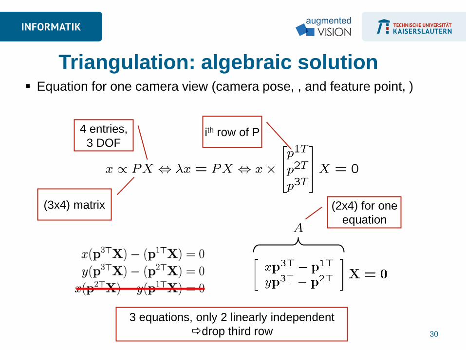
Equation for one camera view (camera pose, , and feature point, )
Triangulation: algebraic solution
ith row of P 4 entries,
3 DOF
(3x4) matrix
3 equations, only 2 linearly independent
drop third row
(2x4) for one
equation
31
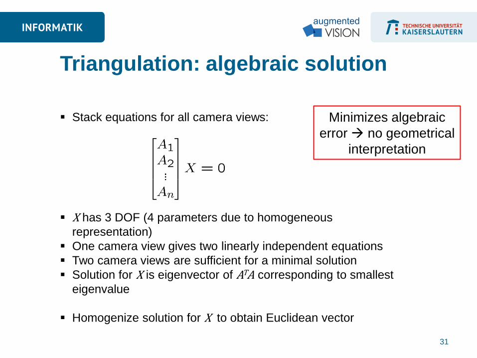
Stack equations for all camera views:
X has 3 DOF (4 parameters due to homogeneous
representation)
One camera view gives two linearly independent equations
Two camera views are sufficient for a minimal solution
Solution for X is eigenvector of ATA corresponding to smallest
eigenvalue
Homogenize solution for X to obtain Euclidean vector
Triangulation: algebraic solution
Minimizes algebraic
error no geometrical
interpretation

P´X
P´ P
32
Estimate 3D point , which exactly satisfies the supplied camera
geometry and , , so it projects as
𝑥 ∝ 𝐶 𝑥 ′ ∝
where 𝑥 and 𝑥 ′ are closest to the actual image measurements.
Triangulation: minimize geometric error
Assumes perfect camera
poses!
d(x,x̂)2 + d(x',x̂')2
subject to x̂ = PX̂ and x̂' = P'X̂
Nonlinear problem: can be
solved with e.g. Levenberg-
Marquard parameter
estimation lecture
PX
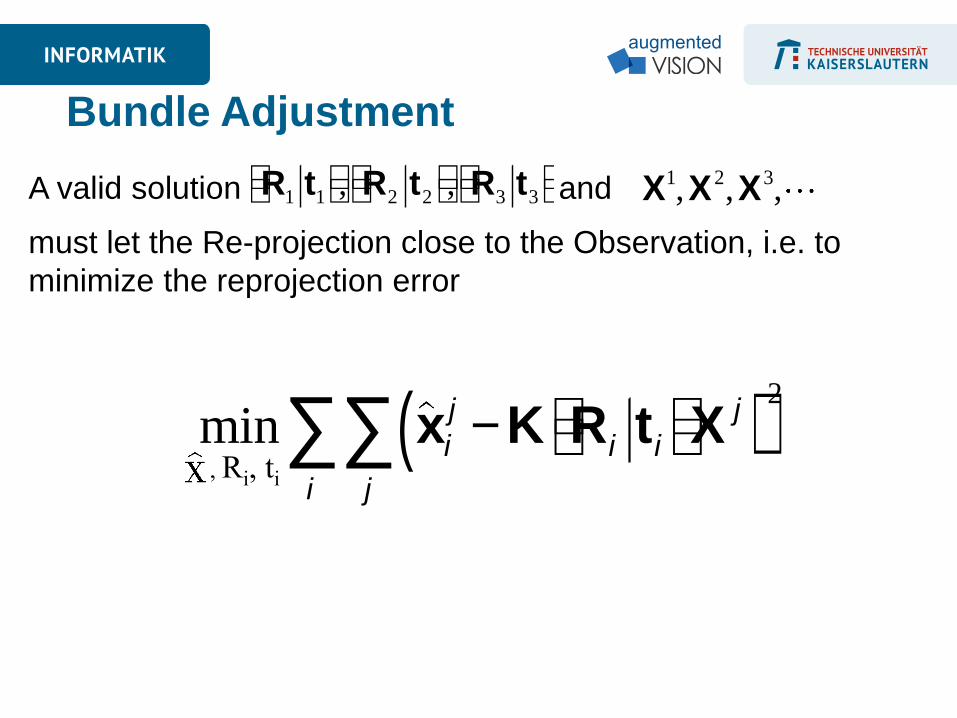
Bundle Adjustment
A valid solution and
must let the Re-projection close to the Observation, i.e. to
minimize the reprojection error
R1 t1éë ùû, R2 t2
éë ùû, R3 t3éë ùû X1,X2,X3,
min xi
j - K Ri tiéë ùûX j( )
2
j
åi
å, Ri, ti

34
Global bundle adjustment:
jointly optimize over all camera poses and
3D points (previous lecture)
Offline drift reduction
Estimate Residual/reprojection error Minimize over
parameter vector containing all camera poses and 3D points
6 parameters for each camera + 3 for each 3D point
parameters must be estimated
matrices are sparse!
Nonlinear estimation problem: use e.g. Levenberg-Marquard
Open source libraries available, e.g. Sparse Bundle Adjustment (SBA)
Over all frames and 3D points

35
+ Minimal parametrization, nice geometric interpretation
- Periodicity, difficult to interpolate
Euler angle representation Sequence not
standardized!

36
A rotation can be represented as a 3D vector direction rotation axis
length rotation angle
Conversion to rotation matrix by Rodrigues’ formula:
+ Minimal parametrization
- Singularity at θ=0
Axis-angle representation r

37
Compromise between rotation matrix and minimal representation
A quaternion is a 4D vector:
Conversion to rotation matrix:
+ Easier conversion to rotation matrix
+ Singularity-free, can be interpolated
- Not minimal, 4 parameters, unit magnitude constraint
Quaternion representation
axis-angle representation

38
The smaller the angle (small baseline, big distance), the bigger
the reconstruction uncertainty!
Triangulation: properties
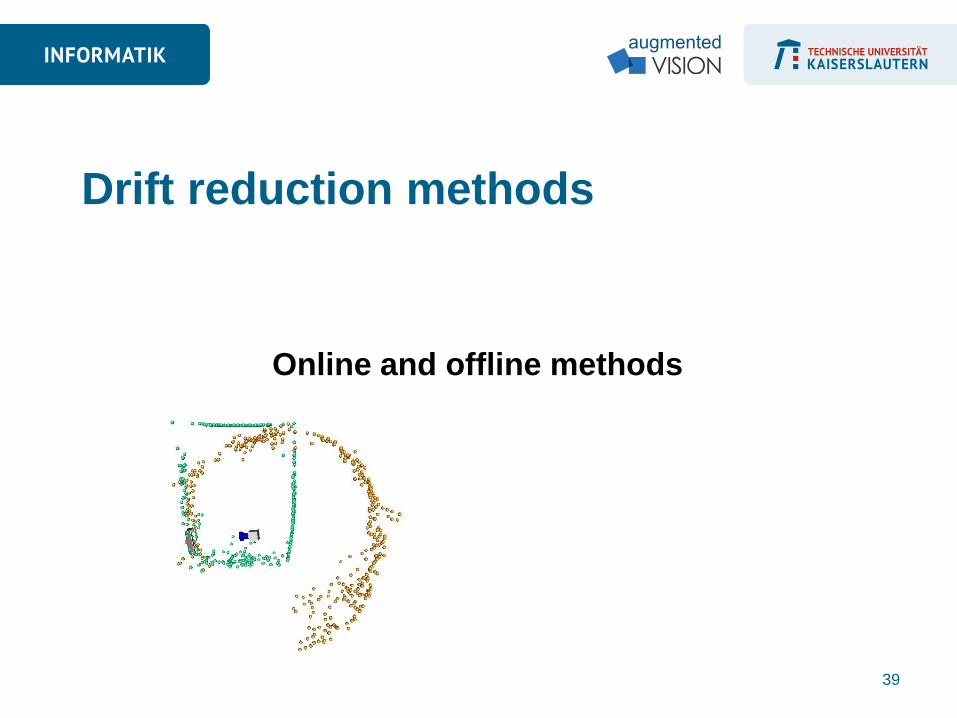
Drift reduction methods
Online and offline methods
39

40
Reduce drift in feature tracking/matching
Extend feature tracks
Reacquire lost features
See topics: image processing, recursive filtering,
advanced visual detection and tracking algorithms
Drift reduction (feature level)

41
Careful (precise, robust) 3D point initialization
How? Triangulate over a whole set of camera views (>> 2)
Enforce a minimal angle θ between view rays
Use RANSAC to eliminate outliers
Use only well reconstructed points for further estimation
Incorporate uncertainties, e.g. simple stochastic model and
WLS estimation lecture on parameter estimation:
All entities modelled as Gaussian random variables
Drift reduction (geometry level)
42
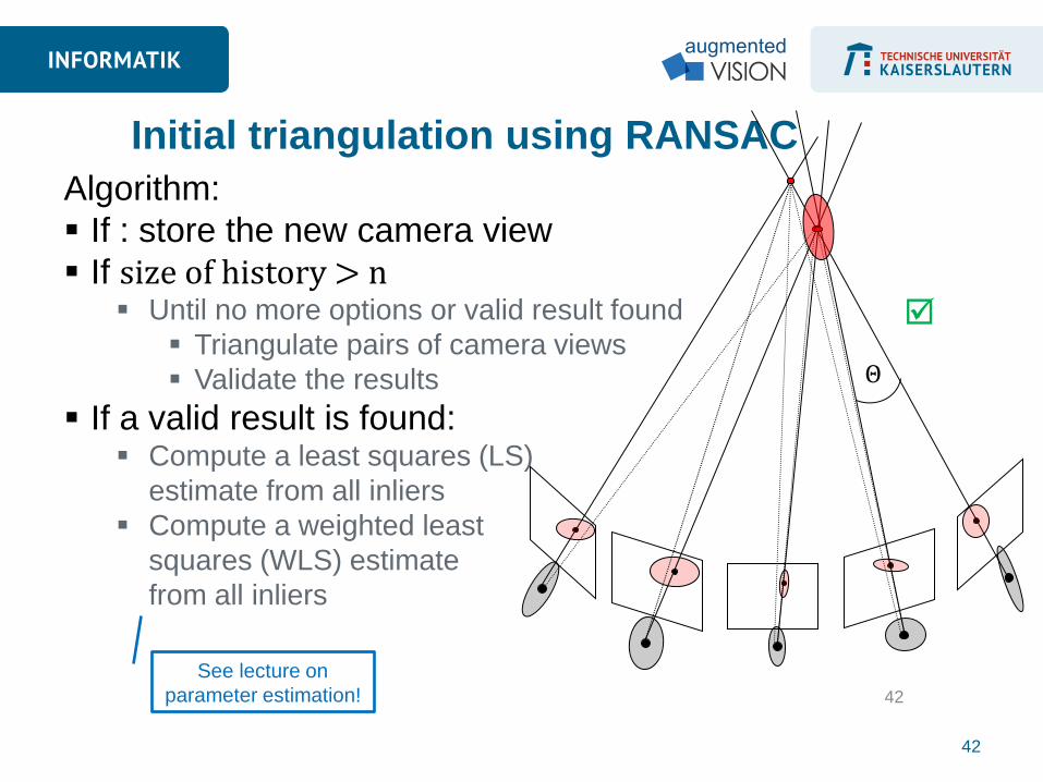
Algorithm:
If : store the new camera view
If size of history > n Until no more options or valid result found
Triangulate pairs of camera views
Validate the results
If a valid result is found: Compute a least squares (LS)
estimate from all inliers
Compute a weighted least
squares (WLS) estimate
from all inliers
Initial triangulation using RANSAC
42
See lecture on
parameter estimation!
Θ

43
Incorporate new camera view, each time the feature is
observed in an image
Methods: Repeated triangulation
Recursive filtering
(e.g. extended Kalman filter)
3D point refinement

44
Results: online SAM (360° rotation)
With drift reduction Without drift
reduction

State-of-the-art approaches
Published at International Symposium on Mixed and
Augmented Reality (ISMAR)
45

46
Title: Online camera pose estimation in
partially known and dynamic scenes
Real-time structure and motion for Augmented
Reality applications
Topics: feature tracking with optical flow,
weighted least squares estimation, recursive
filtering for structure estimation, feature quality
tracking, map management
Bleser et al., ISMAR 2006

47
Bleser et al., ISMAR 2006
2D feature
tracking
(Lost, Valid)
3D
augmentation
•Line model
•Projected 3D
covariances
•Feature
quality (colour
gradient)
External view
on
3D uncertainty
ellipsoids
48
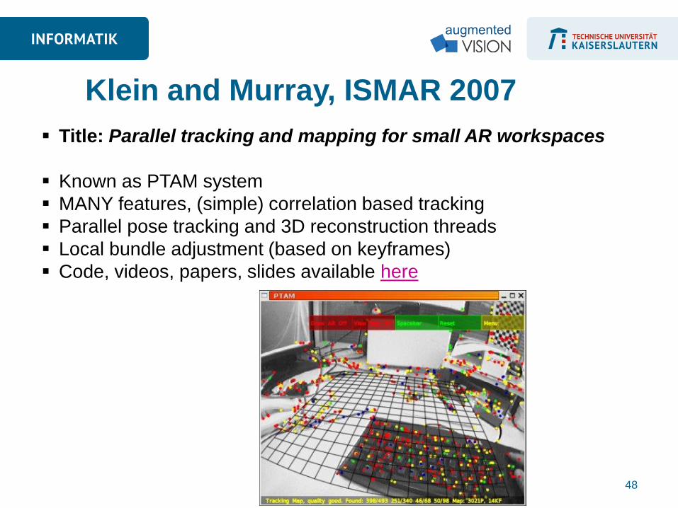
Title: Parallel tracking and mapping for small AR workspaces
Known as PTAM system
MANY features, (simple) correlation based tracking
Parallel pose tracking and 3D reconstruction threads
Local bundle adjustment (based on keyframes)
Code, videos, papers, slides available here
Klein and Murray, ISMAR 2007

49
Title: Wide-Area Scene Mapping for Mobile Visual Tracking
Offline structure and motion tracking model (sparse point cloud)
Online tracking and model extension using mobile devices
Gyroscopes as additional sensors for capturing quick rotations
Server-side localization, jitter reduction
Paper
Video
Code
Ventura and Höllerer, ISMAR 2012

50
Ventura and Höllerer, ISMAR 2012

51
Title: Robust monocular SLAM in Dynamic
Environments
Based on PTAM
Uses invariant features (Scale Invariant
Feature Transform)
Explicitly handles occlusions and moving
scene parts keyframe updating
Variation of RANSAC called PARSAC (prior-
based sampling + enforcing even distribution
of inliers, not just high inlier ratio)
Tan et al., ISMAR 2013

52
Tan et al., ISMAR 2013

Thank you!
Next lecture: dense reconstruction
53