3D Component Method Based on the Rakes - TUT · Henri Perttola 3D Component Method Based on the...

Tampere University of Technology

3D Component Method Based on the Rakes

CitationPerttola, H. (2017). 3D Component Method Based on the Rakes. (Tampere University of Technology.Publication; Vol. 1517). Tampere University of Technology.

Year2017

VersionPublisher's PDF (version of record)

Link to publicationTUTCRIS Portal (http://www.tut.fi/tutcris)

Take down policyIf you believe that this document breaches copyright, please contact [email protected], and we will remove accessto the work immediately and investigate your claim.

Download date:15.04.2020

https://tutcris.tut.fi/portal/en/publications/3d-component-method-based-on-the-rakes(d35dac84-3f5a-4c0c-9a0f-e2f4e26cb60a).html

https://tutcris.tut.fi/portal/en/publications/3d-component-method-based-on-the-rakes(d35dac84-3f5a-4c0c-9a0f-e2f4e26cb60a).html

Henri Perttola3D Component Method Based on the Rakes

Julkaisu 1517 • Publication 1517

Tampere 2017

Tampereen teknillinen yliopisto. Julkaisu 1517 Tampere University of Technology. Publication 1517 Henri Perttola 3D Component Method Based on the Rakes Thesis for the degree of Doctor of Science in Technology to be presented with due permission for public examination and criticism in Auditorium F110 at Frami, Seinäjoki, on the 1st of December 2017, at 12 noon. Tampereen teknillinen yliopisto - Tampere University of Technology Tampere 2017

Doctoral candidate: Researcher Henri Perttola

Research Centre of Metal Structures, Seinäjoki Faculty of Business and Built Environment Tampere University of Technology Finland

Supervisor: Professor Markku Heinisuo Research Centre of Metal Structures, Seinäjoki Faculty of Business and Built Environment Tampere University of Technology Finland

Pre-examiners: Professor Buick Davison Department of Civil and Structural Engineering University of Sheffield UK Professor Jani Romanoff Department of Mechanical Engineering Aalto University Finland

Opponent: Professor Ian Burgess Department of Civil and Structural Engineering University of Sheffield UK

ISBN 978-952-15-4054-7 (printed) ISBN 978-952-15-4068-4 (PDF) ISSN 1459-2045

ABSTRACT

There are not practical design tools adequately available for the three-dimensional (3D) modelling and

analysis of the structural steel joints. Especially, the missing guidance given in the standard has negative

influence on the engineering practice. A motive for this research is to develop the analysis technique for the

3D design of the steel joints. The basic idea is to decompose the analysed joint into the key components,

which play the essential role in the joint response to the given loads, and to replace it with a mechanical

system, which comprises these components. A component ideology of this kind is in accordance with the

component method introduced in EC3 (Section 6 of EN1993-1-8), which includes no instructions for 3D

design of joints. However, there are no obstacles to employ the component ideology in the joint analysis

whether the mechanical model describes the one-, two- or three-dimensional response. In this thesis, the

component method of EC3 is the starting point for the development of the analysis tools for the 3D design of

joints. The main objective is to show that the suggested 3D model defined in compliance with the component

ideology can be used to the resistance prediction. A mechanical model of the suggested type also offer a

method for determining of the interaction curves based on structural analysis rather that fitting procedures.

The stiffness and ductility aspects are considered as secondary or complementary issues in this work. This is

due to the weaknesses inherited from the prevailing component method of EC3 related to formulations on the

component stiffness and ductility.

In the 3D modeling and analysis, the focus of the research is in the response of the bolted end plates in the

tension zone of a joint. The end plates are typically flanges, which transfer the tension over the joint between

the connected members. The bolt acts as tension bolt whilst the end plate has a character of the plate in

bending. The bolted end plate connection can be used in many types of joints like beam-to-column joints,

beam and column splices and column bases. Because the bolted end plate is meant to transfer tension in the

perpendicular direction of the end plate, the shear in the connected member is restricted outside the scope of

this thesis. The splices of a rectangular tube, equipped with the rectangular end plates, are considered as

driving examples in all parts of the thesis. The four-bolt layouts such that the bolts are either symmetrically

placed corner bolts or mid-side bolts in the flanges were studied. The main attention is paid to the end plated

connections with corner bolts whilst the end plate with mid-side bolts can be seen as a reference case. The

resistances of the bolted end plates are derived by the yield line theory in accordance with the upper bound

theorem of the plasticity theory such that this procedure is embedded in the determination of the resistance of

the bolted end plate based on EC3.

The 3D component method was investigated by analyzing the end-plated splices of the rectangular tube

under biaxial bending, which stand for a genuine three-dimensional problem not reducible in the lower

dimensions. The related task was to assemble a mechanical system of components replacing with the

considered splice and solve the problem. The compression components are much stiffer in comparison with

the tension components such that only the location of the resultant force in the compression zone is decisive.

Thus, the properties of the tension components are in the main role in the splice behaviour. In order to study

the validity of the computed results, the test series was arranged on the tube splices under weak axis and

biaxial bending. The experimental validation data was enlarged to the case of the arbitrary biaxial bending

through the numerical analyses supported by the tests. The splices used as the specimens in the tests

corresponds the driving examples. In addition to the main objective, which was the resistance prediction by

the 3D component method, the physical character of the response of the considered end-plated rectangular

tube splice is investigated experimentally and numerically. The arranged tests on tube splices have an

inventive character and no biaxial joint tests like them have not been done before. In the numerical analysis

on the considered splices, the described nonlinear features were the plastic material behavior including strain

hardening, contacts between the end plates and geometrically nonlinear description of the deformations in

the strongly bent end plate and in the bolt when necking. Some of the complementary results based on

numerical simulation are described only in the appendices of the thesis.

Keywords: component method, design of structural steel joints, three-dimensional modelling and analysis,

joints with bolted end-plates, end plate connections, rectangular tubes, bending tests, three-dimensional finite

element analysis,

PREFACE

This study was carried out in the Research Centre of Metal Structures at the Tampere University of

Technology (TUT). The research centre is located in Seinäjoki and it is a part of the University Consortium

of Seinäjoki (UCS), which represents a multidisciplinary scientific community related to five Finnish

universities. The associated projects of this centre were funded by the Regional Council of South

Ostrobothnia, and the European Regional Development Fund (EFDR) during 2009-2013. In addition,

companies (Rauta) Ruukki and Mäkelä Alu (from Alajärvi) are participants in the financing of the research

center. The tests described in the empirical part of the dissertation have been arranged in the testing

laboratory of the Seinäjoki University of Applied Sciences (SEAMK). The usage of the numerical analysis

program ABAQUS was available for academic research by CSC (IT Centre for Science) administered by the

Finnish Ministry of Education and Culture. The arranged tests were financially supported by the Seinäjoki

Region Business Service Center (SEEK). I am thankful for the personal grant from The Confederation of

Finnish Construction Industries RT (CFCI).

I would like to thank my supervisor, professor Markku Heinisuo, for directing me to this interesting field of

joint research. I express my gratitude to Mr Jorma Tuomisto and Mr Veli Autio (SEAMK), who helped me

with the tests and to Mr Jukka Pajunen (SEEK) affected to the positive decision on the financing of the tests.

Very special thanks go to Mr Veli Pajula, who gave invaluable help when the problems turned out with the

computers were solved successfully. I would like to present my gratitude to Dr. Olli Kerokoski, whose

approving attitude and personal choice helped the financing of this study. I give my appreciation to Mrs

Hilkka Ronni and Mr Keijo Fränti as colleagues in research and very fine companionship, especially then we

shared the same room in the research Centre. Unfortunately, I had no colleagues here in Seinäjoki in last two

years during this work. I had possibility to participate an interesting journey to the international conference

of connections in steel structures arranged in Timisoara, Romania and it was delightful to see the enthusiasm

of the colleagues specialized in the research of structural steel connections. In addition, an evening in the

vineyard in Romania was the most enjoyable experience. Finally, I would like to send special greetings to

Mr. Kari Virtanen because of the refreshing talks during the coffee breaks in Frami.

During this work, I have lived together with my loveable wife and our two children in Seinäjoki, the centre

of South Ostrobothnia. Seinäjoki offers, first of all, a clean and safe living environment for families with

children. It is, in additions, a nice town with joyful events, particularly, in the summer time. The flexible

practice in cycling in the streets of this town speaks for the tolerant spirit in the traffic culture.

Frami, Seinäjoki 2017

Henri Perttola

3D-COMPONENT METHOD BASED ON THE RAKES

ABSTRACT

PREFACE

CONTENTS

1 SCOPE AND OBJECTIVES OF THE STUDY ............................................................................... 1

1.1 Introduction .................................................................................................................................... 1

1.2 Approach through the component method ...................................................................................... 2

1.3 Research questions .......................................................................................................................... 4

1.4 Methods and tasks ........................................................................................................................... 6

1.5 Outlines of the thesis ....................................................................................................................... 7

2 RESEARCH ISSUES, DEFINITIONS AND LITERATURE ......................................................... 10

2.1 Introduction to component method ............................................................................................... 10

2.1.1 Classification of the component method of EC3 ........................................................................ 11

2.1.2 Mechanical models ..................................................................................................................... 12

2.1.3 Tension in the end-plated connection ......................................................................................... 14

2.1.4 Compression in the end-plated connection ................................................................................. 16

2.2 Basic concepts related to the research tasks .................................................................................. 16

2.2.1 Starting point .............................................................................................................................. 16

2.2.2 Rakes 16

2.2.3 End plated splices of rectangular tubes ...................................................................................... 20

2.2.4 Four-bolt layouts and T-stubs ..................................................................................................... 21

2.2.5 Biaxial bending, genuine 3D problem, interaction curve ........................................................... 22

2.2.6 Local and global approach ......................................................................................................... 23

2.2.7 Splice problems .......................................................................................................................... 25

2.3 Experimental and numerical methods, literature review ............................................................... 26

2.3.1 Introduction ................................................................................................................................ 26

2.3.2 Experimental research ................................................................................................................ 27

2.3.3 Numerical methods, verification and validation......................................................................... 29

3 EXPERIMENTAL RESEARCH ..................................................................................................... 32

3.1 Introduction to the arranged tests .................................................................................................. 32

3.1.1 Dimensions of the specimens and main factors ......................................................................... 34

3.1.2 Material properties ..................................................................................................................... 37

3.2 Testing arrangements and procedure ............................................................................................. 39

3.2.1 Biaxial bending tests .................................................................................................................. 40

3.2.2 Weak axis bending tests ............................................................................................................. 43

3.2.3 Procedure .................................................................................................................................... 43

3.2.4 Testing programme ..................................................................................................................... 44

3.3 Test results ..................................................................................................................................... 45

3.3.1 Measured and computed quantities ............................................................................................ 45

3.3.2 P-v curves and observations ....................................................................................................... 46

3.3.2 Rotational behaviour of the splices in the tests .......................................................................... 50

3.3.3 Failure modes ............................................................................................................................. 54

3.4 Comparison and remarks ............................................................................................................... 59

3.4.1 Comparison with Wheeler’s tests ............................................................................................... 59

3.4.2 Remarks ...................................................................................................................................... 60

4 NUMERICAL ANALYSIS OF THE TUBE SPLICES ................................................................... 62

4.1 Introduction ................................................................................................................................... 62

4.1.1 Special features of the considered splice problems .................................................................... 62

4.1.2 Elastic-plastic model .................................................................................................................. 64

4.1.3 FE analyses by ABAQUS .......................................................................................................... 65

4.2 Structural models ........................................................................................................................... 66

4.2.1 Modelling of contacts according to their roles in the splice ....................................................... 66

4.2.2 Simplified bolt geometry ............................................................................................................ 68

4.2.3 Structural symmetry ................................................................................................................... 69

4.2.4 Structural model for splice in axial tension ................................................................................ 70

4.2.5 Structural model for splice under biaxial bending ..................................................................... 73

4.3 Discrete model ............................................................................................................................... 78

4.3.1 Discretization, chosen elements ................................................................................................. 78

4.3.2 Elementary problems for verification ......................................................................................... 80

4.3.3 Convergence tests on elementary bolt problems ........................................................................ 82

4.3.4 Convergence tests on splice in axial tension .............................................................................. 89

4.3.5 Remarks ...................................................................................................................................... 95

4.4 Validation and exploitation of the FE model ............................................................................... 96

4.4.1 Introduction ................................................................................................................................ 96

4.4.2 Simplifications and checks ......................................................................................................... 97

4.4.3 Bolt model ................................................................................................................................ 100

4.4.4 Splice model: P-v curves .......................................................................................................... 103

4.4.5 Splice model: M-θ curves ......................................................................................................... 112

4.4.6 Remark on the computed M-θ curves ....................................................................................... 120

4.5 Failure curves for arbitrary biaxial bending ................................................................................ 121

4.5.1 Definitions and procedure ........................................................................................................ 122

4.5.2 Failure curves for splices S1 to S4 ........................................................................................... 124

4.6 Remarks ..................................................................................................................................... 128

5 3D COMPONENT METHOD ...................................................................................................... 129

5.1 Aims and definitions, approach with the rakes ............................................................................ 129

5.2 Components in strong axis bending of a tube splice ................................................................... 131

5.2.1 Basic components in the tension zone ...................................................................................... 132

5.2.2 Basic components in the compression zone ............................................................................. 134

5.2.3 Bending of the splice ................................................................................................................ 134

5.2.4 2D rake ..................................................................................................................................... 136

5.3 T-stub analogy ............................................................................................................................. 137

5.3.1 Yield line analysis .................................................................................................................... 137

5.3.2 Procedure and examples ........................................................................................................... 138

5.3.3 Modified EC3 yield patterns .................................................................................................... 141

5.3.4 Particular mechanisms for the tension flange with the corner bolts ......................................... 145

5.3.5 Decisive mechanisms ............................................................................................................... 150

5.4 Tension components of splices S1 to S4 ..................................................................................... 150

5.4.1 Effective lengths ....................................................................................................................... 151

5.4.2 Resistances and determining mechanisms ................................................................................ 153

5.4.3 Component stiffnesses .............................................................................................................. 155

5.5 3D component model of the tube splices .................................................................................... 156

5.5.1 Decomposition.......................................................................................................................... 156

5.5.2 Potential and active components .............................................................................................. 158

5.5.3 Failure of the rake ..................................................................................................................... 160

5.6 Results and validity of the 3D component method ..................................................................... 161

5.6.1 Resistances and reserves of the splices .................................................................................... 161

5.6.2 Moment-moment interaction curves......................................................................................... 165

5.6.3 Validity of the resistance prediction by the rake model ........................................................... 168

5.6.4 Remarks on ductility and FE simulations ................................................................................. 169

6 CONCLUSIONS ............................................................................................................................ 171

6.1 Empirical study............................................................................................................................ 171

6.2 Numerical study .......................................................................................................................... 172

6.3 3D component method ................................................................................................................ 173

6.4 Final remark ............................................................................................................................... 174

REFERENCES

APPENDICES

A1 3D PLASTICITY MODELS

A1.1 Classical metal plasticity .............................................................................................................. 1

A1.2 Stable material based on work hardening ..................................................................................... 1

A1.3 Construction of the 3D constitutive models ................................................................................. 3

A2 STRESS-STRAIN CURVES

A2.1 Tensile test .................................................................................................................................... 1

A2.2 Curves with continuous yielding .................................................................................................. 3

A2.3 Curves with discontinuous yielding ............................................................................................. 7

A2.4 Stress-strain curves of the splice parts ........................................................................................ 10

A3 CONTACT MODELS AND ANALYSIS METHODS

A3.2 Contact constraints ....................................................................................................................... 1

A3.3 Approaches to contact description ................................................................................................ 3

A3. 4 Contact constraint enforcement methods .................................................................................... 4

A4 FE SIMULATIONS, CONTACTS AND PRYING ACTION

A4.1 Splice model ................................................................................................................................. 1

A4.2 Comparisons between contact analysis methods .......................................................................... 3

A4.3 Contacts caused by pre-tensioning and prying ............................................................................. 4

A4.3 Splice response during necking .................................................................................................... 6

A5 FE SIMULATIONS, TENSION COMPONENTS

A5.1 Quarters Q1 to Q4 ........................................................................................................................ 1

A5.2 Computed P-u curves ................................................................................................................... 3

A5.3 Resistances ................................................................................................................................... 4

A5.4 Stiffnesses, fitting procedure ........................................................................................................ 5

A5.6 Bolt forces ................................................................................................................................... 8

A5.7 Effect of the weld dimensions ...................................................................................................... 9

A5.8 Effect of the pre-tensioning ........................................................................................................ 10

A6 FEM SIMULATIONS, BIAXIAL BENDING

A6.1 Splice S1 in axial tension ............................................................................................................. 1

A6.2 Splice S1 under biaxial bending ................................................................................................... 2



A7 SOLUTION PROCEDURE

A7.1 Nonlinear formulations ................................................................................................................. 1

A7.2 Discretized problem ...................................................................................................................... 2

A7.3 Solution procedure .................................................................................................................. …..3

A8 ELEMENTS

A8.1 Element selection .......................................................................................................................... 1

A8.2 Avoiding volumetric locking ........................................................................................................ 2

A8.3 20-node quadratic serendipity element… ................................................................................. …2

A9 CONVERGENCE TESTS

A9.1 V&V ......................................................................................................................................... 1

A9.2 Errors ......................................................................................................................................... 1

A9.3 Convergence tests. ........................................................................................................................ 3

1

1 SCOPE AND OBJECTIVES OF THE STUDY

1.1 Introduction

In the analysis of a structural problem, all the features including the geometry, kinematics,

loading and material behaviour should be described as three-dimensional (3D) as they really

are. In engineering practice, however, the reduction into lower dimensions is usually required

in order to obtain tractable problems, which also concerns the structural steel joints. The

analysis model, which is able to describe the actual 3D behaviour, is needed when the

problem is not reducible in two- (or one-) dimensional one. A non-reducible problem is called

a genuine 3D problem in this study. The 3D finite element analysis is a typically used

approach in those cases. In addition to the use of heavy FE analysis, practical methods are

requited in the design process of structural steel joints. In the design standards including EC3,

however, the instructions for the analysis of the bolted joints, which are in focus in this thesis,

are directed mainly for the 2D design whilst the proper guidance for the 3D cases is missing.

The 3D problems of the joint design are inevitably present with the space frames. For the 2D

analysis of the plane frames, the behaviour and loading of the members and joints are

described in the in-plane conditions. A deviation from the in-plane conditions due to the

loading or to the intrinsic, asymmetric response of the member (or joint), leads to the 3D

problem with the out-of-plane conditions. For example, the transverse forces in respect to the

plane of the frame together with the in-plane forces cause biaxial bending in the joints. In any

case, an engineer must be ready to design not only the “in-plane joints” of a plane frame but

also the joints in 3D because of their out-of-plane responses. A typical example on a joint

with 3D loading combination is the splice or base of the corner column, which is common to

the two orthogonal frames of the skeleton. A joint can be designed for pure biaxial bending or

for combined biaxial bending and normal force when the shear force is negligibly small. In

addition, a connection can be designed for the pure bending also when the shear force is

transferred over the joint through other parts of the joint (than those transferring tensile or

compression forces), which are intended particularly for that purpose. Particular parts for

shear of this kind are typically used in beam-to-column joints and in column bases.

A conceptual design approach for the 3D joint behaviour under generalised loading has been

suggested by Sim es da Silva (2008). Sim es da Silva proposed the adoption of the principles

of the component method introduced in Eurocode 3 (EC3) as suitable for the 3D joint design.

Generalised forces are simplified representations of the stress state in the structural members

such as beams or columns. The generalised forces in a massive type of a prismatic member

possibly present in 3D frame analysis are the axial normal force, two rectangular components

of the biaxial bending moment, two associated shear components and torsional moment. In

the case of thin-walled members, other generalized forces like bimoment should be taken into

account. The amount of potential 3D joint problems is naturally very large because of the

endless variety of possible joint geometries and loading histories. In this thesis, the choice of

the developed method for 3D joint analyses also falls upon the component method of EC3

partly because of its systematic and generic character and partly because of its position as a

standardised method. The component method is based on the approach that the same (basic)

components can be identified in different joint problems provided that these components have

similar roles in the joints they belong to. The properties of the actual component in the

considered joint can then be determined in compliance with the procedures introduced to the

basic components in the standard. Thus, the same (basic) component can be utilised with

https://en.wikipedia.org/wiki/Cauchy_stress_tensor

https://en.wikipedia.org/wiki/Structural_element

https://en.wikipedia.org/wiki/Beam_theory

2

different types of joints and their variations under different loading cases based on the

analogy between the responses of the actual joint parts and the corresponding components. In

principle, a relatively small number of different basic components allows the analyses of a

vast amount of joint problems with varying layout and loading. It is emphasized that the

components introduced in the prevailing EC3 have the ability to carry uniaxially acting

forces. Consequently, these components can be used in a joint resisting axial force, pure

bending or combined biaxial bending and normal force in compliance with the component

ideology, such that they are compression or tension only components. The plastic deformation

makes the joint problem as nonlinear such that the principle of superposition cannot be used.

The interaction curves defining the allowed combination of (proportional) loading of the joint,

for example, in the case of the rectangular components defining biaxial bending resistance can

be determined through the models based on the component ideology. A mechanical model

defined in compliance with the component method offers a physical approach such that there

is a correspondence between the model and the actual structure instead of the pure fitting

procedure of a mathematical formulation to the test results.

This dissertation is intended to be a part of the larger research through which the three-

dimensional analysis methods for design of structural steel joints are developed. Hopefully

this work can offer support for the development of the component method of EC3. The idea

of this study originally came from the component based modelling of the base plate joints of

tubular columns (Laine, 2007). The main objective was then in the flexible modelling

technique not in analyses of genuine 3D problems. In 2010, the research project of 3D

modelling was launched based on Professor Markku Heinisuo’s initiative in the Tampere

University of Technology. In this study, the driving examples are the rectangular tube to the

end-plated splices of a rectangular tube. Thus, the steel-concrete connections are replaced by

the pure steel-steel connections in which case the tests are much simpler to arrange. The

modelling of the concrete in compression and bent base plate in the compression zone could

then be eliminated. The splice tests were arranged as three-point bending tests corresponding

the (genuine) three-dimensional problem of the tube splices under biaxial bending. It is

emphasized that these biaxial bending tests has a character of pilot tests because no separate

joint tests of this kind have been arranged before. In the 3D research project, the end-plated

splices of rectangular tubes under biaxial bending have also been investigated in fire

conditions. The fire tests have been described by Ronni et al (2012). It should be mentioned

that also the tube splices made of aluminium have been tested during the project.

1.2 Approach through the component method

The analyses and detailing of the (steel) joints are often laborious and time-consuming. An

ideal engineering toolbox for the design of structural steel joints should be suitable for all

types of joints and their variations in arbitrary loading cases. The toolbox should include also

the joints, whose behaviour is dominated by the three-dimensional (3D) phenomena.

Provided that the computational costs are not limited, advanced numerical 3D stress analyses

can be employed in the case of almost every imaginable structure or joint. However, the

practical tools needed in practical 3D design of steel joints are inadequate or sometimes

entirely missing. An ideal 3D analysis method should give sufficiently accurate results, which

are obtained through reasonable computation effort. A rational and uniform approach to joint

design, independently on the required dimensions, would greatly improve this part of the

design practice. It would also be desirable if the physics behind the analysis was seen as the

response of the physical model of the joint. According to thinking of this kind, for example,

3

the assumed interaction curves between the associated forces defining, the resistance of the

joint for the certain loading combination (like normal force and bending moment) should be

described by the physical model instead of the procedure, where the interaction curve is just

assumed in advance. The compatibility of the 3D method with the instructions of the

prevailing design standards written for the two-dimensional joint design would be most

desirable. The enlargement of the standard then is straightforward, and moreover, the large

research behind the in-plane formulations of the standard could then be exploited when the

enlargement to the 3D design is developed. In any case, the systematic and general method

for the 3D analysis of joints is missing in engineering practice yet.

The 3D component model for the joint analysis can be associated with a mechanical system

comprising components representing the deformable parts of the considered joint. The

suggested 3D model is called a rake in this thesis and the basic concepts related to the rakes

are explained in Section 2.2.2. The identification of the components must be followed by the

determination of their properties described by the deformability curves, which define the one-

dimensional force-displacement relations of these components. The deformability curves are

assumed to be independent on the responses of the other components. The components of the

rake resist the loading of the joint in compliance with the requirements of compatibility and

equilibrium set for the mechanical model standing for the considered joint. Thus, the response

of the whole joint is presented as a combination of the responses of the individual

components. The one dimensional components do not know if they are parts of the 1D, 2D or

3D rake, which can be utilized when the 3D component method is developed. If the actual

deformability curves of the components of the rake were known, the full response of the joint

could be solved, in theory, such that the (initial) stiffness, resistance and ductility would be

also known. In the component method of EC3, the stiffness in the initial state and resistance

of the components and joints are evaluated based on the elasticity and plasticity theory,

respectively, without the knowledge of the full deformability curves of the components. The

ductilities of the components, defining their ability to deform plastically, are neither known.

Then the full response and the ductility of the joint (rotation capacity) cannot be determined

by the rake model. Whilst the resistance of the components can expectedly be predicted

simply and reliably by the plasticity theory methods, the stiffness of the components should

be derived according to the rules of the elasticity theory, which results in complicated

analyses in the most of the practical cases. In this thesis, the resistances of the components

and joints are in the principal interest, whilst (initial) stiffness and ductility are left to the

minor role. At the limit sate of the joint, the elastic deformations are usually much smaller

than the plastic ones. The resistances can be approximated based on the yield mechanism such

that the internal work done by the elastic deformations is neglected. The theoretically limiting

case is the rigid-ideally plastic behaviour, where any movement is not possible before the

appearance of the yielding mechanism. Then the resistances of the components (and joins) are

treated as independent of their stiffnesses. On the other hand, the resistances, defined through

elastic-plastic type of analyses, change usually only slightly when the component stiffnesses

are varied. In the most practical cases, the stiffness values can be replaced by the tentative

values based, for example, on a civilised guess, the resistance can still be defined

approximately right.

The simplified mechanical model itself is assumed to be geometrically linear. The materially

nonlinear behaviour of the joint can be described by the nonlinear deformability curves. In

theory, also the nonlinearity associated with the mutual dependence between the deformable

curves, which is neglected here, could be taken into account through the deformability curves.

The fundamental precondition set for the model is that the model should be capable of

4

resisting the applied loads (Section 2.2.2). In this study, the procedures and formulations of

the component method introduced in Part 1-8 of EC3 (EN1993-1-8, 2005) are taken as the

starting point when the simplified model is developed for the 3D analysis. The resistance

predicted by the component method is based usually on the limit loads of the components,

which can be evaluated reliably through plasticity theory. Of course, instability or material

fracture can be the possible reasons for the loss of load carrying capacity of an individual

component, which should be taken into account. Moreover, the determination of the ductility

of the component is not included in the EC3 formulations. In the standard, ductility of certain

types of joints (rotation capacity) is seen to be as sufficient when the conditions related to the

component, the resistance of which governs the (bending) resistance of the whole joint, are

satisfied (Section 6.4 of EN1993-1-8). The ductility aspect in the component model of EC3 is

not fully explained and it must be further investigated (Feldman et al 1996). In the

component method of EC3, the stiffnesses of the components are usually based on the

strongly idealised elastic models, which may give, expectedly, coarse predictions. An

important example is a bent end plate, which is a typical deformable part in the tension

component indentified in a bolted end plate connection. The stiffness formulations suggested

for a bent end plate in EC3 are based on the beam model instead of the proper analysis of the

associated two-dimensional plate problem. In addition, the effect of the deviations from the

nominal initial state is not taken into account by the stiffness formulas of EC3 for the flanged

end plate connection in the tension zone. As a result, the initial stiffness of the whole joint can

be evaluated unreliably when flanged end plate in tension has as a significant role in the joint

behaviour. If the stiffness model is not reliable, in general, neither the analysis of a frame

based on the actual stiffness of its joints is reliable. It should be mentioned that the semi-

continuous elastic design based on the stiffness model of EC3 (BS EN 1993-1-8) is not

allowed according to the UK national Application Document just because of the unreliability

of the EC3 stiffness predictions. In any case, the component method seems to be nowadays

the only candidate for the unified design method of the structural steel joints. The

development of the ductility and stiffness formulations in question would require a research

effort including large and expensive empirical programs. Programs like these would probably

provide cooperation between many researchers in order to be accomplished properly. The

resistance prediction based on the component method seems to be more fruitful or promising

research area including issues proper for a single dissertation. The resistance formulations are

based on the plasticity theory, which offers a simple and reliable way to evaluate the

resistances.

1.3 Research questions

The first selection is to take the component method of EC3 as a starting point for the study.

This was done despite the obvious deficiencies of this method when predicting the stiffness

and ductility as explained above. However, the component ideology is very attempting due to

its general character as suitable for the modelling of joints of almost any kind with varying

layouts and loads. The objective of this thesis is to take a step toward to the three-dimensional

component method intended for the design of structural steel joints; consequently, the

research tasks will be harnessed to this purpose. In order to conceive the required tasks, a

general question is presented first as follows:

(i) Is it possible to predict the behaviour of a structural steel joint under arbitrary static

loading in 3D by the simplified mechanical model defined consistently with the component

method?

5

The set comprising of all the cases, which can be covered by question (i), is too large to be

tractable. Without restrictions, there is a very large amount of different joints and loading

cases to be involved in the study. Thus, the scope of the research must be limited in order to

replace question (i) with a practical one. In this thesis, end-plated splices of rectangular tubes

under biaxial bending are considered (Figures 2-8 and 2-9). This selection is related to the

arranged tests by which the validity of the model can be investigated. The idea is to define a

specimen and testing arrangement such that the (pure) tension and compression components

analogical with those introduced in EC3 can be used in the analysis of the corresponding

problem of the tube splice under bending. In biaxial bending, the initially double symmetric,

bolted tube splice loses its symmetry already at the onset of loading because of the non-

symmetric behavior of the bolted fastener in tension and compression. In any case, the

superposition principle cannot be utilized through dividing the problem as two orthogonal

bending problems due to the nonlinearity: thus, no reduction into the two-dimensional

bending model is possible. As a result, the capability of the three-dimensional model to

describe the response of the end-plated splice to biaxial bending in the arbitrary direction

should be studied as a genuine three-dimensional problem. Because of the tubular shape of

the considered beams, the components of the component method introduced in EC3 are

formally outside the application area of the method. However, the general principles of the

component method prevail despite the formal limitations of the standard. The principal focus

will be in the resistances of the tube splices whilst the stiffness and ductility are in the

secondary role in this study. In compliance with the above restrictions, the considered subset

of all possible cases is reduced such that it stands for a tractable question:

(ii) Is it possible to predict the moment resistance of an end-plated splice under

(monotonically increased) biaxial bending in an arbitrary direction by the simplified

mechanical model defined consistently with the component method?

In order to answer this question, the primary task is to define the 3D component model (rake)

such that the guidelines of the predominant standard are followed as far as possible. The new

components required in the analysis of the considered joints are suggested exploiting the

procedures of the standard. The main interest will be in the resistances of the individual

components and, moreover, on the resistances of the studied splices, whilst the stiffness (and

ductility) of the components and splices are considered only as complementary issues. The

aim is to show that the simple rake model can predict the resistance of the splice under

arbitrary biaxial bending in compliance with the component method. In order to study the

validity of the suggested model, the test series on the tube splices under biaxial bending was

arranged. In principle, the numerical analysis methods can be utilized in order to enlarge the

pure experimental validation data. The complete and general evidence on the validity of the

3D component method is not tried to reach by this study, which is the first of its kind. If the

positive answer to question (ii) were attained, it would stand for a small subset of those cases

required for the answer of question (i). In spite of this, any positive answer to question (ii),

suggest the suitability of the component method for 3D joint analysis, whereas a negative one

would cause, at least, a reason for a comprehensive explanation. The complete answer of

question (i) further requires the research on the stiffness and ductility aspects, which are only

coarsely touched on in this work. It is emphasized that the deficiencies of the stiffness and

ductility model are inherited from the component method of the prevailing standard taken as

the starting point of this study. Before the 3D component method could be added to the EC3,

the more comprehensive evidence about its validity is needed. This is not possible through an

individual thesis like this but requires many more studies.

6

A 3D model, which is capable of predicting the resistances, can be exploited, in principle,

also to determine the interaction curves of the joints. This property, which is related to the 3D

models, can be seen as a complementary motive to this study on the 3D component method.

The splices used as the specimens in the tests have been considered in all parts of the thesis.

In addition to the main intentions to study the validity of the 3D component method, the

physical character of the response of the considered end-plated rectangular tube splice is

investigated experimentally and numerically.

It must be acknowledged that, in compliance with the modern conception of the character of

scientific research, the aims and tasks were gradually developed and focused during the

research to those described above. The progression related to the steps in the different stages

of this study is not described in detail. However, the set questions basically correspond to

those asked at the beginning of the study, when Prof. Markku Heinisuo suggested the themes

for the research.

1.4 Methods and tasks

The methodology employed in this thesis consisted of the analytical part including modelling

and analysis by the component method, experimental investigation and numerical analysis

part. In this study, the direct plan was to form a simplified mechanical model for the end-

plated rectangular tube splices under arbitrary biaxial bending, in compliance with the

principles of the component method. Then the validity of the model was investigated against

the experimental data, which was enlarged numerically. The related tasks in the experimental

and numerical parts of the thesis and those associated with the modelling and analysis of the

tube splices by the component method, serve the main objective set by the question (ii). The

observations on the behaviour of the investigated splices in the tests and the additional FE

simulations can be understood as complementary results to those serving directly to the

principal aim.

Analytical part. The modelling and analyses of the studied tubes splices under biaxial

bending comprise a task in which the component ideology is utilized. The components of the

model have to be identified, the new components defined and their properties evaluated

consistently with the procedures of the standard as far as possible. The new tension

components were defined for end-plated splices with four-bolt layout assembled with

symmetrically placed corner bolts (Figure 2-9) or mid-side bolts. The resistances of the

components are obtained as the plastic limit loads. For steel plates in bending in the tension

zone of the splice, the yield line theory is employed. The tension components are described

analogically with the basic T-stubs. This approach is similar whenever the corresponding

tension component is modelled as an end-plated connection whether it is in the tube splice or

other type of the joint. There are no instructions in the standard regarding how the

compressive components should be described in the case of biaxial bending. Then, the task is

to define the components consistently with those components readily available in the

standard. Altogether, the idea is to utilise the formulations and procedures introduced in the

prevailing standard insofar as is possible in this task.

Experimental study. In this study, the comparison between the results predicted by the 3D

component method for tube splices under biaxial bending (structural entity) and tests results

was preferred, whilst no tests for the separate components were arranged. Because no biaxial

7

bending tests on tube splices were found in the literature, the new tests had to be carried out.

A relatively small number of tests, which are inventive in their character, with the modest

instrumentation were arranged because of the limited resources. The tests were arranged as

three-point bending tests on a simple beam with a splice at mid span. Then the biaxial tests

can be conducted such that the free transverse movement of the jack acting at mid span is

allowed. The premise for a simple interpretation of the test results is that the transverse

displacement and torsional deformations remain so modest that the testing arrangement does

not change essentially during the tests. By choosing the specimen such that the permanent

deformations concentrate on the splice whereas the tube remains in elastic range, the tube

deformation predicted by the beam theory can be excluded from deformations (rotation) of the

splice itself. The tests were arranged under load control. Therefore, the initial stiffness and

resistance of the specimen could be determined by these tests, whereas the post-critical

response was out of their reach. Another motive for the tests is to gain a better understanding

about the behaviour of the tube splices under biaxial bending. The influence of the end plate

thickness (or stiffness in respect to the bolt stiffness) on the splice behaviour, and especially

on the failure modes, is the question of main importance. The end plate thicknesses varied

while the bolts (size and grade) are kept the same. The aim is to observe the failure modes of

the specimens and compare them with those of the (equivalent) T-stub in order to clarify

whether the T-stub analogy can also be exploited in the case of the corner components.

Numerical methods. The response of the structures can be investigated, in general, by

numerical simulations when the tests are difficult to arrange or too expensive, or when the

quantities are cumbersome to measure. In principle, the analysis model should be validated

against the test results. In this study, the considered tube splices were modelled and analysed

as three-dimensional structures by the three-dimensional finite element method (3D FEM).

The arranged tests were simulated and the validity of the model was investigated against these

tests. The experimental data was enlarged numerically as supported by the tests results. The

numerical simulations of the studied splices can be also utilised when the special features in

splice behaviour are investigated. In any case, the enlargement of the test data by numerical

means for the splices under arbitrary biaxial bending is the principle objective of the

numerical analyses in this thesis.

The geometrically nonlinear description of the kinematics must be included in the analysis of

the tube splices. This concerns, especially, the strongly bending end plates and necking of the

bolts. The elastic-plastic 3D FE analysis with the description of the strain hardening

phenomena is embedded in the von Mises type of metal plasticity model. The chosen material

model based on the plasticity theory represents the well-known techniques that have been

employed largely in the numerical analyses. The used contact analysis model, which is based

on the frictionless normal contact, also represents the classical approach. These methods are

usually available in the tool palette of the advanced FE programs including ABAQUS v. 10.6

used in this study. Verification of the numerical model has been investigated through

convergence tests, by which the required mesh densities were determined. In the considered

splice problems, both the locally and globally instable behaviours are expected to appear.

Particularly, necking of the bolts may occur also when globally unstable behaviour in not yet

present. Then, the selection of the solution procedure for successful analysis is not self-

evident. To avoid difficulties with the convergence in the (equilibrium) iterations and the

complexity of the solution procedure, displacement control is preferred. The equilibrium

configuration can then be found through the Newton-Rhapson type of iteration in every taken

increment. The structural models in question are suitable for the displacement controlled

solution procedure, because the external load can be easily extracted from the analysis results

8

based on equilibrium equations. It should be mentioned that elastic-ideally plastic analysis

fails to describe the strain hardening behaviour of the strongly bent end plates and necking of

the bolts both of which play the important role in the studied splices.

1.5 Outlines of the thesis

Overview. In the thesis, the suitability of the component method for the three-dimensional

analysis of the tube splices was studied. Both experimental and numerical methods were used

in this study. The biaxial and weak axis bending tests were arranged, and their results were

further enlarged in the case of arbitrary biaxial bending by means of the numerical analysis in

order to investigate the validity of the suggested models based on the rakes. In the used

approach, the answer to the research question(s) on the suitability of the component method

into 3D analysis is investigated through these individual examples called driving examples. A

positive answer would be deemed as the evidence of the need for further development of the

studied method based on the rakes. Hopefully, this study will be pioneering in the area of 3D

joint research by the component method.

Sections. The objectives and scope of the thesis are given in Section 1. The basic concepts

and research issues, including the idea of the simplified mechanical model (rake), have been

introduced in Section 2. The detailed presentation of the 3D component model for a tube

splice itself is not discussed until Section 5, where the main results of the study are also

presented. Section 3 presents the experimental part of the thesis, where the arrangements of

the three-point bending tests and their results are described. Six conducted tests correspond to

four different splices, which are used as the driving examples throughout the thesis. The

numerical models of the tube splices and the analyses results are presented in Section 4,

where the used structural models are presented. For the verification of the FE model,

elementary convergence tests have been conducted with the chosen elements; as their

outcome, sufficiently dense element meshes are found. The validity of the numerical analysis

results is investigated by comparing them with the test results. The moment-moment

interaction curves for biaxial bending are determined based on the numerical model and

supported by the tests. In Section 5, the rakes are defined in compliance with the component

method for the considered splices under arbitrary biaxial bending. The tension and

compression components and the associated formulations not included in the standard are

described. The special attention is paid to the resistance of the tension component in the case

of symmetrically placed corner bolts such that particular yield line mechanisms are suggested

The used approach is based on the analogy between the actual corner component and the T-

stub. The resistances and failure modes of the components are determined. Finally, the

resistances of the splices were estimated by the rake model. The validity of the 3D component

method is investigated against test results and “numerically expanded validation data” for

arbitrary biaxial bending. In Section 6, the conclusions and remarks on the study are given

Appendices. The used material and contact models were introduced in Appendices A1 to A3.

The stress-strain curves are presented in A2. The finite element simulations of splices under

tension or under biaxial bending are discussed in Appendices A4 to A6. Based on the FE

simulations, the response of the considered splice has been followed over the maximum limit

point up to the descending stage of the load. The contact behaviour and prying phenomenon

in the splice under axial tension are considered in Appendix A4. Appendix A5 is devoted to a

study on the response of the separate tension components when compared with the results of

the elastic-plastic analysis of the splice in axial tension. The effects of the size of the weld

9

(between the tube and end plate) and the bolt pretension on the behaviour of the tension

component were also examined. In Appendix A6, the splices under biaxial bending are

considered. In Appendix A7, the used solution procedure is described. The selection of the

element type and the principles behind the convergence tests on the FE models are discussed

in Appendices A8 and A9, respectively. Although the aspects gathered in the appendices can

be seen as the necessary to be understood by the numerical analyst, they play only a

secondary role in respect to the main objectives and scope of the thesis. Consequently, they

are set in the appendices not to disturb the main objectives of this study.

10

2 RESEARCH ISSUES, DEFINITIONS AND LITERATURE

2.1 Introduction to component method

The component method introduced in the EC3 represents a practical engineering approach to

predicting the response of structural steel joints. The component method is introduced in the

part 1-8 of EN 1993-1-8. It should be noted that the “revised annex J” of European pre-

standard (ENV 1993-1-1 1994) essentially included the prevailing version of the component

method with some differences in the stiffness model (Feldman et al 1996). In any case, there

is not a general and comprehensive presentation on the theoretical bases of this method. The

author has become acquainted with the component method first by reading the descriptions

about the component method applied to the base plate joints of columns. The associated

papers are published in a special issue of HERON (Wald et al 2008a; Wald et al 2008b;

Steenhuis et al 2008; Jaspart et al 2008; Gresnigt et al, 2008). These articles can be read as a

general introduction to the component method when the base plate joints have the roles of the

“driving examples”. The described procedures analogical with that, which is required in the

analysis of end plate connections whether they are parts of the column base, column-to-beams

joint or the splices of beams and columns. This is in accordance with the component ideology,

which can be associated with the principle that the similar components can be identified in

different joint types on the certain conditions set for the considered joints. The principal

formulation used in EC3 for the tension components of the end plate connection, which have

a special role also in this thesis can be found in Zoetemeijer’s researches (1974, 1990). It

should be noted that the above mentioned researches (e.g. Zoetemeijer, Jaspart, Weynand and

Wald) had an important impact on the standardisation of the component method in EC3. The

component method and its ideology have been explained by Jaspart (1991, 2000). Compact

descriptions of the safety consideration and stiffness model of the EC3 joints are presented,

respectively, by Feldman et al (1996) and Weynand et al (1996). In the thesis written by

o Coelho (2004), the component method is described in addition to the characterization

of the ductility of bolted end plate beam-to-column connections.

In EN 1993-1-8, the component method is presented under the heading “Structural joints

connecting H and I sections”, which excludes other profiles outside the formal application

area of the standard. In Figure 1.2 of EN 1993-1-8 (see Figure 2-1), a plane frame is shown in

order to point the “joint configurations” belonging to the application area of the standard. In a

frame like this (constructed of I or H profiles), the beams act typically as members under

strong axis bending and columns under combined normal force and strong axis bending.

Consistently, the guidance given in Section 6 of the standard concerns mainly beam-to-

column joints (number 1 in the figure), beam splices (3), column splices (4) and column bases

(5). Double-sided beam-to-column and beam–to-beam “minor-axis joint configurations” are

also included in the case of balanced moments (shown in the figure at bottom). However,

there is no reason why the component ideology should be restricted in these cases. It should

be also remembered that engineers have always been utilized the “idea of decomposition” of

the structures into separately analysed parts in their computations independently of the

component method of EC3. The general aspects of the joint design are discussed as related to

the design of structural moment resistant joints by Jaspart (2000). He suggests that the design

concepts, in general, should provide “the unified design approach for the structural joints

whatever their loading, their configurations and the nature of their constitutive materials

11

are”. The systematic approach based on the component method, where any joint can be seen

as a set of individual basic components, is in line with thinking of that kind.

Figure 2-1. Joint configurations of the application area according to EN1993 1-8.

2.1.1 Classification of the component method of EC3

The research on structural steel joints and the related development of the design methods have

been active in the last few decades. The rotational behaviour of a beam-to-column connection,

i.e., its response against pure strong axis bending, represents a problem type studied most.

The different methods, intended for the modelling of the rotational behaviour, are categorized

by Nethercot and Zandonini (1989). They described an approach based on the simplified

analytical model. This approach comprises the stages:

identification of major sources of deformations in the connection

elastic analysis of the initial loading phase, concentrating on the key components to

predict initial connection flexibility

plastic mechanisms analysis for the key components to predict ultimate moment capacity

of the connection

verification of the resulting equations against test data (NOTE: the used term should be

“validation” instead of according to the V&V terminology, ASME V&V 10-2006)

12

Description of the moment-rotation behaviour of the connection by curve fitting using the

calculated initial stiffness and ultimate moment capacity in suitable expressions.

Jaspart (2000) completed the classification of Nethercot and Zandonini by adding the

component method in its place as a method representing a simplified analytical model. When

the rotational response of a joint, that is, its moment-rotation curve, is determined through the

component method of EC3, the above described procedure is followed. The stiffness and

resistance of the joint are evaluated independently of each other. The initial stiffness of the

joint is as dependent on the geometry (lay-out) of the joint and on the elastic modulus and

independent of the strength properties (or safety factors). On the other hand, the (moment)

resistance of the joint is determined according to the appropriate plastic limit state assumed to

the joint. Finally, the moment-rotation behaviour is described such that the transition from the

initial (elastic) state to the ultimate (plastic) limit state is interpolated without actual analysis

of the corresponding mechanical model. Consistently, the mechanical model comprised of the

components of the splice is utilized separately when the stiffness and resistance is calculated

by the component method.

2.1.2 Mechanical models

In order to form a mechanical model for a joint, its deformable (or key) components must be

identified in the decomposition process. The components are the deformable parts of the joint

model whilst rigid links are connecting these components. Thus, the mechanical system

replacing the joint is defined by the locations and properties adopted for the components.

When the deformability curves, which describe the force-displacement relations of the

components, are introduced, the response of the joint could be followed through the structural

analysis of the system. The response of the model is determined by the equilibrium and

compatibility conditions the latter of which are defined in compliance with the movements of

the rigid links. In the case of steel joints, the actual components have nonlinear character with

increasing plasticity. In principle, the elastic-plastic analysis of the decomposed model could

give the “full response” of a joint including its resistance as the plastic limit load. An

incremental and iterative solution procedure is required then due to the material nonlinearity

in spite of the geometric linearity assumed for the model itself. Of course, the resistance of the

component may be caused by the other reason than yielding. Then the additional conditions

for failure must be defined. The spring systems replacing a joint can be divided into two

categories according to the character of the deformability curves, such that:

In the mechanical model, the deformability curves describe the actual behaviour of

the components. A model like this can be constructed, in principle, when the

deformability curves are based on tests or numerical analyses supported by tests.

In the simplified mechanical model, the idealised deformability curves are used

instead of the actual ones.

The motives of the analysis significantly affect the choice of the deformability curves: the

simplified model can be utilised in the design or it can be selected purely from the theoretical

point of view. The actual deformability curves are not usually known and their determination

by tests may be a laborious process. In this study, the simplified mechanical models are

utilised when the 3D component method is formulated. The component method as it is

introduced in EC3 can be used then as a starting point. The analogical formulas and

procedures as in the standard are employed when it is possible. In order to demonstrate the

spring systems used as joint models, two examples are considered. In these, the deformable

13

components are replaced by springs, whose properties determine the behaviour of the joint.

Both of the models have been exploited in the structural steel research, which is motivated by

the aims of developing the component method of EC3.

The first example is a spring system used for the prediction of the moment-rotation response

of a base plate joint illustrated by Figure 2-2 (Jaspart & Vandegans 1998). In the model, the

springs represent the key components whose deformations (extensions, rotations) are

constrained through the movements of one or more rigid parts or links connecting them. The

essential phenomena should be taken into account in the behaviour of the column base. These

include the interaction between the base plate and concrete, the anchor bolt in tension and its

anchorage in concrete, the formation of the plastic hinge in the column, the base plate in

bending and the related development of the yield line in the extended part of the plate. In the

joint model, the deformable components are the extensional springs for the deformation of the

column in tension and compression (number 1 in Figure 2-2), for the deformation of the

anchor bolts and base plate subjected to the anchorage force in tension (2), for contact

between the base plate and concrete in compression (3) and, finally, the rotational springs for

the bending deformation of the extended base plate in the compression zone (4).

Figure 2-2. The column base (joint nr. 5 of Figure 2-1) and the associated spring system are shown

side by side. This schematic drawing reproduces the original one shown in (Jaspart et al 1998).

The loading case with combined bending and axial force can be analysed by this model. The

incremental and iterative solution procedure must be exploited because of the nonlinear

constitutive laws of the components. Due to the complicated behaviour of a column base, the

creation of a simple model by which an analyst can obtain accurate results is a contradictory

task. Better accuracy can be attained by increasing the density of the associated contact

components between the base plate (steel) and concrete. On the other hand, a relatively small

number of springs is allowed so that the model does not lose its simplicity. If the focus is in

the development of the scientific tool for predicting the nonlinear (rotational) response of the

column base, the complexity will not matter. The validity of the model was investigated by

comparing the full moment-rotation curves obtained by the model with the experimental ones

by Jaspart and Vandegans (1998). The comparisons interceded on behalf of the mechanical

model as a reasonable tool for research purposes although it may be too complicated to be

utilized in practical engineering work. This model is likely to be, anyway, computationally

more efficient than those models based on advanced numerical procedures.

Another example of a spring system, which is intended to the analysis of the beam-to-column

joints, is shown in Figure 2-3 (Sim es da Silva et al 2000, 2001a). In this model, the bilinear,

elastic-plastic type of deformability curves ( - , shown on the right side of the figure) are

used for the key components. For components in the tension zone, the first subscript of the

stiffness coefficients refers to the component and another one to its position in the joint.

14

In compliance with the numbering used in Table 6.1 of EN 1993-1-8, the identified tension

components (defined per bolt row) are the column web in transverse tension (i = 3), column

flange in bending (4), end-plate in bending (5) and bolts in tension (10). In the compression

zone, correspondingly, the relevant components are the column web panel in shear (1) and

column web in transverse compression (2). The components related to the beam are omitted

here (beam flange in compression (7) and beam web in tension or compression (8)). In

bilinear formulation, the initial stiffness ( ) of a component determine the response in the

elastic range after which the post-limit stiffness ( ) prevails. This can be modelled

by two springs in series, where the first represents initial stiffness and the second (spring

constant ) becomes active once the yield strength ( corresponding the knee point) has

been obtained. The collapse displacement ( ) defines the end of the post-limit step. The

moment-rotation curve of the joint ( - ) can be followed by the incremental analysis of the

spring system. Even the analytical solutions can be obtained, in principle, including the

equivalent post-buckling behaviour.

Figure 2-3. A beam-to-column joint and the associated spring system are shown abreast on the left

side and the deformability curve of a component is shown on the right (Sim es da Silva 2001a).

The spring system of Figure 2-3 represents a model, where the idealised deformability curves

are employed. Through this model, the post-limit stiffness and ductility of the end-plate

beam-to-column steel joints under pure bending can be studied. Based on the materially

nonlinear analysis of the spring system, the maximum available rotation ( ) of a joint can be

solved by the incremental and iterative procedure (or even analytically). Sim es da Silva et al

(2002) suggested a concept of a joint ductility index defined as a ratio / between the

joint rotation in failure ( ) and rotation ( ) obtained when the first component reached its

elastic limit associated with the knee point of the bilinear model. The joint ductility index can

be used as a decisive parameter when the sufficiency of the rotation (deformation) capacity is

judged in respect to the chosen analysis type (elastic, plastic) of the considered frame. This

must be done, in principle, if the post-limit responses of the joints are utilized.

2.1.3 Tension in the end-plated connection

The T-stub analogy can be employed in the analysis of the joints containing the deformable

parts, such that equivalent T-stub replaces the actual tension component in the end plate

connection. The requirement of the equivalence is set regarding both for the (initial) stiffness

and failure mode. The failure modes of the “elementary T-stub” are described below. In

principle, it is immaterial whether a tension component like T-stub (with local character) is

used in 2D or 3D model. The associated basic component can be idealised in the same way in

both of these cases.

15

mode 2

PP

mode 1 mode 3

P

T-stub. The tension component replaced by the T-stub is represented by the basic

components “end plate in bending” (number 5 in Table 6.1 of EN 1993-1-8) and “bolts in

tension” (10) in series. It is noted that, the basic components “column flange in bending”,

“flange cleat in bending” and “base plate in bending” act in the same way as the “end plate in

bending” in the tension zone. It is required that the equivalent T-stub must have the same

failure mode and resistance as the actual component. The failure modes of the T-stub in

tension (against force ) are illustrated in Figure 2-4 (Table 6.2 of EN1993-1-8). These are

Mode 1: Complete yielding of the flange,

Mode 2: Bolt failure with yielding of the flange and

Mode 3: Bolt failure.

Figure 2-4. Failure modes of the T-stub. Modes 1 and 2 occur with prying.

Mode 1 takes place in a T-stub, which has flexible flanges in respect to the bolts. The plastic

hinges (= yield lines) in the flange only define the plastic mechanism. In mode 3, which

usually occurs in the case of stiff flanges (in respect to the bolts), yielding of the bolts solely

determines the limit load. Mode 2 represents the intermediate behaviour between modes 1 and

3 including yielding, which occurs in both the bolts and flanges. In modes 1 and 2, the prying

phenomenon takes place such that the contact force between the flange and foundation is

equilibrated by the additional bolt forces. Here, “additional bolt force” refers to a bolt force

that is larger than one can expect by the equilibrium assumed without prying. In the mode 1

mechanism, the prying action occurs such that the prying force reaches its theoretical

maximum value restricted by the complete yielding of the plate. The prying action appears in

mode 2, but the yielding of the bolts prevents the prying force from reaching its theoretical

maximum value. In addition to modes 1 and 2, a mode without prying (not drawn in Figure 2-

4) can take place based on the mechanism, where plastic hinges are formed only in the flange

near the web of the T-stub. The bolt flexibility (elongation length) must be then larger than

that required for the bolts able to force the prying action to occur. This mode is typical for the

base plate joints with the anchor bolts. When the resistances of an actual component and T-

stub are equated, the effective length of the equivalent T-stub can be, in principle,

resolved. The equivalent T-stub replaces the actual T-stub in the joint. The equivalent T-stub

gives the resistance of the component associated with the smallest value attained with modes

1 and 2. If mode 3 is decisive, the resistance value of the tension component depends on the

bolt resistance(s) rather than the equivalent length.

When a flanged connection is subjected to tension, an internally indeterminate prying force

may develop as described above. The physical nature of the prying phenomenon is described,

inter alia, by Henning Agerskov (1976, 1988). Agerskov presented diagrams by which the

character of the prying effect can be studied quickly without lengthy calculations or advanced

numerical analyses. The role of prying action in HSS (=Hollow Steel Section) flange-plated

16

connections in axial tension is studied by Willibald et al (2002). According to it, the normal

force resistance of the connection, which is less than or equal to the total resistance of the

bolts due to the prying action, can be evaluated by the presented thumb formula. It is noted

that the occurrence of prying is taken into account in modes 1 and 2 in the stiffness

coefficients introduced in EC3.

The failure modes of a T-stub are classified in the prevailing EC3 in essentially the same way

as suggested by Zoetemeijer (1974) when he presented “a design method for the tension side

of the statically loaded, bolted beam-to-column connections”. Zoetemeijer derived his

formulas for the effective lengths of the equivalent T-stubs so that the resistance and stiffness

of the unstiffened column flange could be evaluated. No such design tool had been developed

before to be used in the case of a relatively flexible flange used as a tension connection

(without the additional support provided by the stiffening plates).

2.1.4 Compression in the end-plated connection

When the bending response of an end plated connection is investigated, the compressive

forces are transferred by contacts between the plated parts. The distribution of the contact

forces in the compression zone determines, in theory, the magnitude and position of the

compressive resultant force, which equals the tensile resultant force. In Table 6.15 of

EN1993-1-8, the locations of the centre of compression for deriving the design moment

resistances are defined for the typical beam-to-column joints. For the extended end plate joint,

for example, the centre of compression is in line with the mid-thickness of the beam flange in

the compression zone.

2.2 Basic concepts related to the research tasks

2.2.1 Starting point

An enlargement of the component method into three-dimensional joint analysis was suggested

by Heinisuo et al at (2009) Nordic steel construction conference in Malmö in 2009. This can

be seen as a starting point to a research project on the 3D modelling of the end plated steel

and aluminium joints in ambient and steel joints in fire conditions. The researchers of this

project were led by Professor Markku Heinisuo from the Tampere University of Technology.

In addition to many conference papers, which enlightened the intermediate results of this

project, the related themes are presented in the journal papers (Heinisuo et al 2012a, 2012b,

2014). The suggested 3D analyses are based on simplified mechanical models called rakes the

physical basics of which are enlightened next.

2.2.2 Rakes

Spring systems, or rakes, shown in Figure 2-5 are considered. The springs of these rakes are

composed of translational springs at a rigid foundation. The other ends of these springs (when

more than one) are constrained by the rigid links connecting them. The springs are pinned in

their both ends such that they can carry only axial loads. A rake can be used as a model of the

connection when the influence of the transverse forces on the components of the rake can be

neglected, i.e., there is no disturbance due to the transverse forces. The basic joint

components numbers 5 and 10 of EC3 (Table 6.1 of EN1993-1-8) called the “end plate in

17

bending” and “bolt(s) in tension”, respectively, resist only the axial forces in the tension

flange neglecting the transverse loads. A rake comprised of the mentioned tension

components together with those, defined to carry compression, can resist pure bending or

combined bending moment and normal force consistently with the component method of

EC3. In an ideal case, the external loads cause only tension or compression to the components

of the modelled joint such that this joint can directly be replaced by the rake alone. However,

the absence of the shear forces is unusual in the practical joint problem. The transverse forces

can also be neglected when the shear force is carried by the other parts (components) of the

joint than those modelled by a rake. The joint parts, which are intentionally designed to carry

the shear force, are typically used with column bases and beam-to-column connections. Those

components of the joint, which carry the normal forces and bending moment, can then be

modelled as a rake. Altogether, the basic rules of the engineering practice of design must

hold also in this case.

The sequential steps from the uniaxial model to the three-dimensional one can be

demonstrated through three spring systems shown in Figure 2-5. For the present, the springs

can be assumed to be elastic. These rakes represent the simplest models capable to carry loads

in one, two and three dimensions, such that they are statically determinate for the

corresponding loads: normal force, strong axis bending, biaxial bending shown in the figure.

In the one-dimensional model (highest in the figure), there is only one spring, which can resist

a force parallel to the spring itself. This spring force can be understood to be an axial normal

force coming from the connected member. The elongation of the spring defines the

deformation of the model. In the 2D model (middle in the figure), there are two springs

connected by a rigid bar (through hinges). The two end points of the springs must define a

straight line such that , in which case the model can resist combined normal force

and (strong axis) bending moment (M ). The deformation of the 2D model can be

described by the axial displacement and the rotation associated with the bending moment.

Thus, there are the two degrees of freedom in this rake. In the three-dimensional case shown

as the lowest in Figure 2-5, three springs are connected by a rigid plane through the ball joints

such that the endpoints of the springs are not allowed to be in the same straight line (

and so that the model can resist biaxial bending and ), in addition to

the normal force . Biaxial bending is defined by two nonzero components and

, such that the -axis of the rectangular -coordinate system coincides with the axial

direction of the connected member (and springs). Two rectangular rotation components

( and ) and the axial displacement ( ) are required to define the deformed state of the

rake. If any of the springs in the models of Figure 2-5 loses its ability to carry loads, the

associated model turns into a mechanism. In contrast, if extra springs are added, these models

turn into statically indeterminate ones. In the latter case, both equilibrium equations and

compatibility conditions are required in order to solve the spring forces and deformations of

the model. As explained above, the change in the length of each spring is related to the

assessed constraint such that the spring ends follow the movement of the rigid bar or plane

(compatibility demand). It is emphasised that none of the models in Figure 2-5 can resist the

shear forces ( , ) and the torsional moment .

For a rake, the tension-only and compression-only springs can be defined such that they are

active only in tension or compression, respectively. Consistently, a spring is active only if it

carries a force ( ). Those forces present in the active springs must be able to equilibrate

the external loads. It should be noted that the requirement of the minimum amount of springs

in the statically determinate rakes concerns only the active springs. A simplified mechanical

18

h > 0

N

N

M

M

z

x

y

N

x

My

s > 0

s > 0

1D

2D

3D

model can be obtained by adopting elastic–ideally plastic response for the active springs. The

associated rheological models for tension and compression only springs are shown in Figure

2-6. The friction elements determine the plastic resistances of the tension-only and

compression-only springs as ( 0), and ( 0), respectively. Plastic flow happens

only when these values are reached: before that, the components are assumed to behave

elastically. For a compression-only component, it holds that:

,

, (2-1)

, ,

where is the spring coefficient in compression. Correspondingly, for a tension-only

component:

, ,

, (2-2)

,

where is the spring coefficient in tension. Instead of elastic–ideally plastic formulations

of Eqs. (2-1) and (2-2), the deformability curves of other idealised types can be adopted by

which, for example, the ductility of the joint can be investigated according to the principles

suggested by Sim es da Silva et al (2002) discussed above. In theory, the actual deformability

curves could be used for the identified components in order to simulate the joint behaviour for

increasing loads in an accurate way. However, a procedure of this kind would be too difficult

to use in the practice.

Figure 2-5. 1D, 2D and 3D models and the loads they can carry.

A 3D spring system shown in Figure 2-7 is considered as an example of a rake. Let the

properties and placing of the springs to be symmetric in respect to the plane such that the

19

z

x

xM

combined T1 and T2

combined C1, C2 and C3

M = xM

3D model (rake) 2D model (EC3)

C3

C1

C2

T2

T1

O

y

response to nonzero component ( ) is correspondingly symmetric. The active

components only in the rake under bending moment are presented. The movement of the

rigid plane connecting the springs defines the deformation of the rake. This plane can be

replaced by the rigid bars or links drawn from the origin O to the ends of the springs (C1, C2,

C3, T1 and T2) laying all in this plane. The active springs are flagged such that the first letters

C and T refer to compression and tension components, respectively. In principle, the springs

in the compression and tension zone can be projected onto -plane when the response

against is modelled, because the distances to -axis then are the relevant ones. Then the

rigid plane can be replaced by a vertical, rigid bar connecting the tension and compression

components. In Figure 2-7 (on the right), the active components are described by one

compression and one tension spring, respectively, in the tension and compression zone (called

a simplified model in EC3). In the case of biaxial bending and ), the

projected model defined only in -plane is not sufficient to describe the response of the rake

alone because of the structural asymmetry. Due to the compression or tension only properties

of the springs, the activity of each spring must always be checked for the resultant force.

Actually, the possibility of the change in activity (compression or tension) or the onset of the

yielding of the spring must always be taken into account such that the used solution procedure

has to be incremental. The considered rake under bilinear bending (with the springs shown in

Figure 2.6) can be characterised as a genuine three-dimensional problem.

Figure 2-6. Rheological models and the corresponding - curves for a) a component capable of

taking tension only and b) a compression only component.

Figure 2-7. Symmetric rake in respect with -plane (left) and the reduction into 2D model (right).

The 2D and 3D models of Figure 2-7 represent one-layer rakes with the springs only in one

layer between the rigid foundation and the rigid links or plate. In principle, a complex joint

structure could require a spring system, which is modelled as a multi-layer rake with more

20

than one layer of springs (Figure 2-2). In this work, the main attention is focused on joints,

which can be modelled through the one-layer rakes capable to resist biaxial bending. The

normal force is assumed to disappear ( and the shear stresses are omitted. The used

model must be able to describe the behaviour of the considered joint model under arbitrary

biaxial bending and ). The objective is to determine the moment-moment

interaction curve ( – diagram) of the considered joint, such that the answer to question

(ii) set in Section 1.3 can be found. The natural requirement in the development of the 3D

component method is to demand that the 3D model, when reducible into 2D model, should

give the same response to ( as can be attained according to the prevailing

standard. This requirement has been employed when the analysis based on the suggested 3D

rake is formulated. The missing definitions needed for the question (ii) are presented in detail

next.

A rake represents a discrete simplification of reality based on the assumed roles of the

components in a decomposed joint. Each component corresponds a certain entity of the joint

and the assembly of the components represents the whole splice. The accuracy of the analysis

based on a rake depends decisively on that how realistically the properties of the individual

components can be described. A mechanical model with actual deformability curves is, in

principle, a theoretical limit, which is approximated by the solution obtained by the discrete

model with simplified deformability curves. There is no general procedure to create a

successive series with the “denser meshes” in the component method opposite to the finite

element method (FEM). It is emphasized that the correctness of a FE solution can be

investigated through the convergence tests, which are, in general, not reasonable with the

component method. A basic component of the component method has a general character

such that it can be utilized in different joints and layouts to replace the actual components. A

method with versatile basic components of this kind can be described as generic (Heinisuo et

al 2009). The basic components introduced in EN1993-1-8 can be used to characterize one-

dimensional springs needed for the rake model. In principle, these can be used independently

whether the 1D, 2D or 3D model (rake) is considered. If new components are required, these

can be employed provided that their validity can be shown against tests. One must keep in

mind that the component method introduced EC3 is primarily intended as a design tool for

structural steel joints, not as a scientific method for their analysis.

2.2.3 End plated splices of rectangular tubes

In this thesis, the approach to 3D analysis is based on the “driving examples” taken as the

practical objects of the research. These are the end plated splices of rectangular tubes, a

typical one of which is illustrated in Figure 2-8. The flanges without stiffeners may

sometimes be too flexible in practise. On the other hand, due to its simplicity of the

fabrication and assembly, a splice of this kind may be an attempting choice. Their resistance

to biaxial bending is the main objective in this study. In the compression zone of the tube

splice under bending, the forces seek the route through contacts between the end plates. In the

tension zone, the bolts act as tension bolts such that the bolt force (tension) is transferred

through contacts from the bolt head and nut to the end plates. The additional tension in the

bolts caused by the prying action may appear with the associated contacts between the end

plates in the tension zone. The prying action itself is self-equilibrating phenomena: the

additional tension force causes the equal contact force between the end plates. In the tension

zone, the end plate will transfer the tension force to the tube mainly as a plate under bending,

21

whilst the shear and membrane stresses of the end plate are usually in the secondary role

when compared with the bending stresses. The flexible end plate (in respect to the bolts) may

bend significantly, which can usually be associated with a ductile behaviour of the entire

joint, whereas the stiffer end plates indicate, on the contrary, a less ductile response due to the

more decisive role of the bolts. By studying the behaviour of the flanged tube splices, the

essential features typical for the other types of extended end plate connections can be also

revealed.

Figure 2-8. End plated splice with corner bolts for a rectangular tube.

In the experimental part of the thesis, “isolated joint tests” will be arranged on the splices

representing to the driving examples. The three-point biaxial bending tests on rectangular tube

splices were relatively easy to arrange. The dimensions of the studied tubes and their splices

were chosen such that the plastic (permanent) deformations were concentrated mainly on the

splice, whilst the tube remains in elastic range. The response of the splice itself could then be

brought forward through the tests. The transverse horizontal displacements due to the

asymmetric bending related to the primary (vertical) loading remained small enough in these

tests so that the simple interpretation of the test results was possible. Furthermore, these tests

will be simulated computationally through the numerical analysis means by which the

suitability of the tests was confirmed in addition to the observations on the tests. Numerical

analyses for splices under axial tension will also be done as complementary when the physical

character of the considered splices is enlightened.

2.2.4 Four-bolt layouts and T-stubs

To gain familiarity with the special features of the studied end plate connections, the four-bolt

layouts are discussed next. In Figure 2-9, four different double-symmetric layouts of the end

plated connections representing beam-to-beam joints (beam splices), are shown and marked

by the letters A to D. On the left in the figure, the splice of the I-beam is shown (case A),

whilst other cases (B to D) represent the splices of rectangular tubes. It is assumed that the

strong axis bending moment acts on the splices such that the tension zone is lower. The

tensile resultant force in splice A under bending is associated with the forces transferred by

the bolt pair together with the lower flange of the end plate. This can be described by the T-

stub analogy through the component method in accordance with EN1993 1-8 such that the

formal prerequisites are fulfilled: 1) the member type is the right one (I or H section) and the

2) requirement for bolt placing holds ( ). The latter one means that the bolt pair is placed

inside the limits defined by the width of the beam flange. Layouts from B to D represent the

splices of rectangular tubes: therefore, none of them fulfil the formal prerequisites of the

prevailing standard. In the case of layout B, however, an essentially similar tension

component can be identified as in the splice with layout A. In principle, the resistances of the

22

tension flange in layout B can be evaluated by the plasticity theory based on the similar yield

line patterns given in Table 6.6 of EN1993-1-8. The associated stiffness coefficient can be

determined for the tension flanges in splices A or B, in turn, according to Table 6.11 of

EN1993-1-8. The (initial) stiffness of the splice is predicted then through the elastic model,

such that the bent tension flange is described by the kinematics of a beam instead of the two-

dimensional plate model. In the case of splice C with the corner bolts, the analogy with the

layouts A is obviously lost. Most likely, the decisive plastic mechanism giving the minimum

value of the limit load for the tension component (flange with bolts) in splice C is not

included in those available in the prevailing standard and suitable for splice A (or B).

Furthermore, in the layout with the corner bolts, the stiffness of the tension flange is

obviously smaller than in case A with . Thus, poor estimates for both the resistance and

stiffness are expected in the case of the corner bolts by the formulas of the standard meant to

be used in the case of splice A. In layout D, with bolts in the mid-lines of the splice cross-

section, the three lowest “mid-side bolts” are the tension bolts, whilst a single bolt in the

upper flange plays a secondary role in the splice response. In addition, the tension flange with

a bolt does not obviously behave like a tension flange with a bolt pair. A single mid-side bolt

in layout D presumably resists tension more efficiently than a separate bolt in a two-bolt row

placed as in layout A or B. The analogy between the tension flange of splice D and the

tension flange of splice A (or B) is questionable and, thus, the formulations of the standard

cannot directly be used in the case of layout D.

Figure 2-9. Layouts of the extended end plate joints.

The end plate connection with a four-bolt layout of type C or D (indicated by the dashed line

in Figure 2-9) represents a simple construction with an especially easy assembly. These

splices will be considered the driving examples in the thesis. The main interest is in the

behaviour of the tube splices with the corner bolts (layout C), which are outside the

application area of the component method introduced in the prevailing standard as explained

above. It is also arguable if a connection with the mid-side bolts (layout D) can be analysed

by the standard. Thus, the new tension components must be defined in the case of layout C

and, possibly, with layout D. Despite the fact that the thesis focuses on the 3D modelling of

joints, the study of the considered connection types can be seen as an additional objective of

the research.

2.2.5 Biaxial bending, genuine 3D problem, interaction curve

In a generalised 3D loading typically present in the beam analysis, three rectangular

translational and three rotational (generalised) force components can be introduced: the axial

normal force , shear forces ( and ), bending moments ( and ) and torsional

moment ( ). In the case of thin-walled beams with open cross-sections, the bimoment ( ) or

23

some other generalised force may also occur. When the bolted connection of Figure 2-10 is

double-symmetric, the bending moment about the strong axis causes only a rotational

deformation about the strong axis, and, correspondingly, a rotational deformation about the

weak axis is due the weak axis bending only.

Figure 2-10. Resultant bending moment in the arbitrary direction.

In this study, the considered splice model (rake in Figure 2.6) can carry the rectangular

components and of the resultant bending moment . The (pure)

biaxial bending is illustrated by Figure 2-10 such that and represent strong and weak

axis bending, respectively. The angle between the y-axis and the direction of the resultant

moment is . It holds that and , respectively, in strong and

weak axis bending. In the case of biaxial bending ( and ), the connection loses

its symmetry due to the yielding of the components. As a result, a genuine 3D problem is

obtained. The superposition based on the separate solutions for weak and strong axis bending

does not hold.

In the design of the tube splice under biaxial bending, it must be shown that any bending

moment caused by the loading remains on the safe side in respect to the moment-moment

interaction curve - curve) defining the resistance against bending in the arbitrary

direction. On the other hand, through the analyses of the 3D joint model, it is possible to

determine this failure curve of the biaxial bending. Consequently, based on models with this

“in-built ability” to predict the resistance in any direction, the sufficient resistance can be

checked directly. It should be noted that the resistance in question is defined against

monotonically increasing biaxial bending moment.

2.2.6 Local and global approach

The plastic limit analysis based on the yield line theory can be utilised in two alternative ways

when the moment resistance of a joint including end plate connection(s) is predicted. One can

introduce the plastic mechanism for the whole joint at once in a global approach or

decompose the joint into (key) components in compliance with a local approach. In the latter

case, the plastic mechanisms are defined separately for the identified components,

corresponding the component ideology. In the local approach, the idea of the equivalent T-

stub determined for the end plate flange in the tension zone is exploited. Next, both

approaches are described using examples found in the literature. The basics of the practical

yield line analysis are presented, for example, by Chen & Han (1988) and by Szilard (1974).

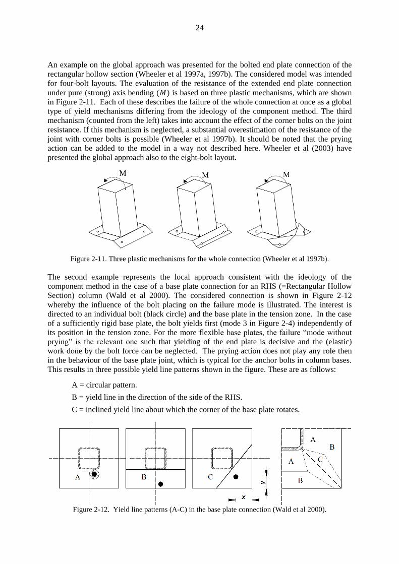
24

An example on the global approach was presented for the bolted end plate connection of the

rectangular hollow section (Wheeler et al 1997a, 1997b). The considered model was intended

for four-bolt layouts. The evaluation of the resistance of the extended end plate connection

under pure (strong) axis bending is based on three plastic mechanisms, which are shown

in Figure 2-11. Each of these describes the failure of the whole connection at once as a global

type of yield mechanisms differing from the ideology of the component method. The third

mechanism (counted from the left) takes into account the effect of the corner bolts on the joint

resistance. If this mechanism is neglected, a substantial overestimation of the resistance of the

joint with corner bolts is possible (Wheeler et al 1997b). It should be noted that the prying

action can be added to the model in a way not described here. Wheeler et al (2003) have

presented the global approach also to the eight-bolt layout.

Figure 2-11. Three plastic mechanisms for the whole connection (Wheeler et al 1997b).

The second example represents the local approach consistent with the ideology of the

component method in the case of a base plate connection for an RHS (=Rectangular Hollow

Section) column (Wald et al 2000). The considered connection is shown in Figure 2-12

whereby the influence of the bolt placing on the failure mode is illustrated. The interest is

directed to an individual bolt (black circle) and the base plate in the tension zone. In the case

of a sufficiently rigid base plate, the bolt yields first (mode 3 in Figure 2-4) independently of

its position in the tension zone. For the more flexible base plates, the failure “mode without

prying” is the relevant one such that yielding of the end plate is decisive and the (elastic)

work done by the bolt force can be neglected. The prying action does not play any role then

in the behaviour of the base plate joint, which is typical for the anchor bolts in column bases.

This results in three possible yield line patterns shown in the figure. These are as follows:

A = circular pattern.

B = yield line in the direction of the side of the RHS.

C = inclined yield line about which the corner of the base plate rotates.

Figure 2-12. Yield line patterns (A-C) in the base plate connection (Wald et al 2000).

25

In Figure 2-12 on the right, the bolt locations are related to areas marked by the capital letters

A to C according to the decisive yield line pattern. The decisive pattern gives the lowest

plastic limit load for the bolt placed at that area. It also corresponds to the shortest effective

length for the equivalent T-stub (defined also in the case of a corner bolt). Mechanism A, with

the circular pattern, dominates the areas near the profile, excluding the “corner area”.

Mechanism B is determining in the area further from the profile next to area A. In the corner

area, mechanism C is decisive. It is obvious that smaller limit loads are obtained with the

bolts in corner area C than in areas A and B when the placing of the bolts are compared in the

same line parallel to the straight side of the rectangular tube. In a parallel line, moreover, the

minimum limit load or minimum effective length for the equivalent T-stub is obtained,

when the bolt is placed in the line halving the end plate corner (dashed line in the figure). In

the case of a bolt in the corner area (C), the effective length is given in the form:

(2-3)

where is a coefficient depending on the dimensions of the base plate and rectangular

components and determine the bolt location measured from the tip of the end plate corner.

According to Eq. (2-3), the bolt in the line provides the weakest resistance for the

associated tension component. The equivalent T-stubs defined in the tension zone can be

exploited when the resistance of the whole joint is evaluated through the component method.

The compression components in the compression zone of the column base are not discussed

here. In this thesis, the local approach is exploited in order to form 3D models for the

considered tube splices.

The above reasoning brings out the character of a corner bolt in the end plate connection as a

disadvantageous structural solution when judged in respect with the resistance of the joint. It

should be noted that also the stiffness of the base plate (in bending) with the corner bolt is

lower than without the corner bolt. In spite of this, the benefit obtained from the easy

assembly due to the corner bolts is sometimes more important. Then, the method for the

analysis of the end plate connection with corner bolts are required although the associated

design rules are missing in EC3. It is emphasized that the special interest is paid to the

resistances of the tension components of the end plate connections in the case of the

symmetrically placed corner bolts (= bolt in the dashed line in Figure 2-12) in Section 5 of the

thesis.

2.2.7 Splice problems

In this thesis, the focus on the static, three-dimensional modelling and analysis of the end

plated rectangular tube splices under monotonically increasing (proportional) loading at room

temperature. The considered problems are divided in the following types:

I) End-plated tube splice under biaxial bending in the arbitrary direction and

II) End-plated tube splice under axial tension.

Problems of types I and II are defined for tube splices, whose properties are the same as those

used in the tests. The associated problems represent the driving examples of the study. It is

emphasized that both of these problems can be modelled through EC3 components, which

carry either tension or compression when active. It is emphasized that no shear is involved in

26

the analyses of these problems of type I and II. The tests consistent with these problems are

described in Section 3 and the structural models for the numerical analyses are defined in

Section 4.

2.3 Experimental and numerical methods, literature review

2.3.1 Introduction

The main objective of this thesis was to develop the 3D component method for the modelling

of steel joints based on the rakes. However, most of the work was included in the empirical

and numerical parts, which only support the principal aim. Tasks presented in these parts were

accomplished in order to determine the resistances of the splices empirically and to enlarge

the purely empirical data by the numerical means. These intermediate results can be utilised

later when the performance of the 3D component method is investigated. However, the

observations on the tests and reasoning based on the numerical models can be seen as the

complementary results of their own shedding light on the physical character of the splice

response.

The conducted joint tests on tube splices under biaxial or weak axis bending , Figure

2-10) represent a new type of tests, whereas the traditional bending tests have usually been

arranged as strong axis tests ( ). In the tests on double symmetric splices, the specimen

is set in the inclined position such that bending in the vertical plane deviates from strong axis

bending. In the biaxial bending tests ( ), the interaction between weak and strong axis

bending cannot be avoided due to the nonlinear and asymmetric character of the splice

response. The weak axis bending test ( ) represents a special case, where interaction

does not appear. The tests are usually expensive and laborious to arrange, which also holds

true in this study. Consequently, it was not possible to investigate biaxial bending in arbitrary

directions through an extensive series of many tests related to the gradually varying value of

the angle . By the numerical simulations, it is possible to replace the testing and, at the same

time, extend the reach of the purely experimental approach. The numerical analysis model

must be verified and validated before it can be used to produce “enlarged experimental data”.

In order to simulate the static response of a tube splice under biaxial bending (type I problem,

Section 2.2.7) or in axial tension (type II problem) in a realistic way through the numerical

analysis, the essential features of the splice behaviour must be identified and embedded in the

used model. The model should be able to describe of 1) the end plate in bending including its

strain hardening stage, 2) the bolts in tension including necking and 3) contacts through which

the contact stresses are transferred over the associated areas in contact. In the splice response

to the monotonically increasing bending moment, the gradually spreading plastic

deformations in the end plates and in the bolts play the main role, such that these two actions

determine the failure mode in an analogical way with the T-stub in tension (Figure 2-4). The

strain hardening of the end plate may have a significant influence when the flexible end plates

bend largely, whereas necking of the bolts(s) typically is decisive in the case of the stiff end

plates. It is emphasises that the simple ideally-plastic models fail to describe realistically both

necking of the bolt and strain hardening of the end plate. In addition to the material

nonlinearity, the geometrically nonlinear behaviour might have a noticeable influence on the

response of the tube splice. The end plate may bend so excessively that the membrane effect

related to the membrane forces in the end plate must be taken into account. Kinematics of the

bolt must be described as nonlinear so that necking can be analysed reliably. In addition,

27

changing contacts represent a cause of nonlinearity, which complicates the analysis. The

contact forces between the end plates in the compression zone are needed when the bending

moment is transferred over the tube splice. In the tension zone, the contact forces between the

end plates equilibrate the additional prying force in the bolts. Thus, both of these interactions

must be described in a reasonable way including the varying contact areas and contact

stresses. It should be noted that the computational efficiency of the obtained numerical

solution may depend decisively on the contact modelling.

Altogether, the three-dimensional, elastic-plastic finite element model able to describe the

geometric non-linearity and contact behaviour is employed for the analysis of the end-plates

tube splices. All features of the modelled structure involving the geometry, boundary

conditions, material behaviour and loading should be presented as discretized for the

numerical model. In practice, the description of the complicated features may lead to

unpractical and heavy models or/and computational problems. The strict modelling of the

structural details is not meaningful provided that the essential behaviour of the investigated

structure can be studied by the lighter models. For example, it is usually reasonable to

describe the bolts without threads in static analysis. The equilibrium path of the splice can be

followed as displacement controlled over the limit load. The actual resistance of the model

must be predicted in the arbitrary direction. The target is then in the moment-moment

interaction curve of biaxial bending for the considered splice. The stiffness predictions

obtained by the model are paid only a secondary attention.

Next, the literature related to experimental and numerical study accomplished in this thesis is

reviewed. The separate 3D joint tests are rarely reported in the area of structural steel

research. Instead, many examples on the 3D FE analyses based on the elastic-plastic models

can be found in the literature. The verification of the discrete model is neglected or they are

passed briefly in some articles, where the elastic-plastic model is exploited in the analysis. For

example, the convergence tests are presented rarely. Of course, the descent presentations can

also be found in this respect. The fluctuating terminology related to the verification and

validation (= V&V) of the computational models can be seen as disturbing. The literature

including the basic concepts required in the verification and validation process is mentioned

at the end of Section 2.

2.3.2 Experimental research

A reason for the missing descriptions of the biaxial bending tests on joints, in general, may be

found in their complexity associated with the inevitable interaction between the strong and

weak axis components of the biaxial bending moment. In spite of this, the flexural behaviour

of joints under biaxial bending can be seen to exemplify an important special case of 3D

loading. In this context only monotonically increasing, proportional loading cases, where the

ratio between the components of biaxial bending is unchanged during the loading, are

concerned. In spite of this, there is an unlimited number of different combinations of biaxial

bending in an arbitrary direction. In any case, the author did not find any test report on end-

plated splices for rectangular tubes under biaxial bending in literature. Thus, particularly

arranged tests were needed for this thesis.

A strong axis bending tests are by far the most usually described static test in the literature

amongst those arranged in order to study the flexural response of structural steel joints. It

represents the in-plane loading conditions exploitable in the analyses of plane frames. In turn,

28

isolated joint tests arranged on joints under loads representing the out-of-plane loading

conditions are quite rare. This holds also with the end plate connections, including the end-

plated splices for rectangular tubes. Celikag and Kirby presented an idea of the out-of-plane

bending and torsional static tests of beam-to-column joints used in the steel frames (Celikag

& Kirby 1987, 1989). They said that “two similar specimens should be loaded up to failure in

different directions to find out the load carrying capacity of the joint in each direction”. They

suggested, furthermore, that guidance (standard) for out-of-plane tests on beam-to column

joints should be developed based on their pilot tests, such that the beam is loaded as a

cantilever instead of the cruciform tests, which rely on the structural symmetry (like minor

axis configurations shown in Figure 1-1) . When the flexural response of a connection is

studied by tests, however, the associated rotation must be extracted, which is not simple in

their testing arrangement, especially, when biaxial bending is concerned. Thus, an out-of-

plane test of this type is not suitable for a biaxial bending test needed now. In the seismic

loading of a steel framework, the loads may arise in almost any possible direction. Reports

describing the damages caused by earthquakes tell the story about the influence of the 3D

loading. The information related, for example, to biaxial bending (in the arbitrary direction)

is, in general, impossible to identify and separate from the data of this kind. The dynamic 3D

loading tests simulating the seismic performance of the structures including structural steel

joints can found in literature. To mention one, an experimental study on column base plate

joints under “cyclic bending about the weak axis” is described in (Lee et al 2008).

A substantial amount of experimental data on the behaviour of the T-.stubs (in tension) is

available in the literature. These tests are more often arranged on T-stubs with roll-formed

profiles than on those put together by welded plates. A test series on T-stub connections made

up of welded plates is described by Gir o Coelho et al (2004). In those tests, most of the

specimens failed by tension rupture of the bolts after the bending deformations of the flange,

such that the gradually increasing plastic deformations of the flange depended in the expected

way on the geometric and material characteristics of the connections. Gir o Coelho et al

(2004) also reported on the “too early” collapses of some specimen, which were due to the

cracking of the plate in the heat affected zone (HAZ). Thus, these tests demonstrate amongst

other things that it is important to do the welding procedure in the right way in order to

achieve a ductile behaviour of the connection. For example, cracking in the HAZ may be due

to the wrong choice of the welding consumable. In any case, Gir o Coelho et al stated that

through proper welds, the designer can ensure that the welded connections do not essentially

reduce the resistance and the deformation capacity of a joint.

Tests on tube splices. Wheeler et al (1997a) have reported on the “bending tests of bolted

end plate connections in cold formed rectangular hollow sections” subjected to pure bending.

These tests were arranged as four-point bending tests on tube splices under strong axis

bending. It is noteworthy that in the case of double-symmetric splices for square tubes, the

difference between weak and strong axis bending disappears. In splices with a four-bolt

layout (type B), the bolts were located outside the edge lines of the tube (i.e., in the corner

area). The associated connections were predominantly semi-rigid, whereas those with an

eight-bolt layout without corner bolts (type A) were, in turn, predominantly rigid according to

the classification scheme suggested by Bjordhovde et al (1990). Tests arranged by Wheeler et

al showed that the rigidity (thickness) of the end plate has an obvious effect on the rotational

behaviour of the splice. The thicker the end plate was, the more rigidly the tested splice

behaved while other factors were held constant. The tests also brought out the larger

flexibility due to the corner bolts. The three failure modes were observed: bolts reached their

ultimate tensile load, the end plate sheared around the tube section and excessive plastic

29

deformation of the end plate occurred in bending. In punching shear, the bottom flange

sheared near the toe of the weld in the tension zone. In the tests of connections with corner

bolts, bolt failure (or failure of threads) was decisive except for in those cases with the

thinnest end plate, whereby the excessive deformation of the end plate took place such that

those tests were stopped before any actual breakage. In the tests of splices with an eight-bolt

layout, either bolt failure or punching shear dominated independent of the plate thickness.

These tests on tube splices were conducted under displacement control. The post-critical

response of the specimen could then be followed in order to investigate the “final failure

modes”. Wheeler et al also analysed the splices numerically by FEM discussed below.

The article titled “Experimental study about bolted HSS flange-plate connections in axial

tension” describes the results of a total of 16 tests on end plated splices for square tubes

(Willibald et al, 2002). In the tested splices, the bolts were symmetrically placed on all four

sides using two different eight-bolt layouts both with and without corner bolts and a four-bolt

layout with a bolt in the middle of each side of the square-shaped end plate. The prying

phenomena, which appear in the splices under axial tension, are of major interest in that

study, where, next conclusions based on the arranged tests are presented. The thickness of the

end plate is the main variable affecting the prying action, which decreases with the increasing

plate thickness. Prying can be minimised by placing the bolts as close to the tube wall as

possible. The longer outreach of a fillet weld in the direction of the flange-plate reduces the

prying somewhat. In the eight-bolt layout with corner bolts, a corner bolt acts less efficiently

than one inside the extended perimeter lines of the tube walls. It should be noted that unequal

bolt loading of this kind is, in general, not desirable. The same themes are considered in more

detail in Silke Willibald’s dissertation (Willibald 2003). She also analysed tube splices by

numerical means as explained below. It is emphasised that the prying in an end-plated splice

under axial tension resembles the prying that can be observed in the tension zone of the same

splice under pure bending.

Ongoing project. Four biaxial ( ) and two weak axis ( ) bending tests with four

different joint layouts on tube splices were conducted for this thesis, where they are described

in Section 3. These tests are also included in the separate test report (Perttola & Heinisuo

2011) with six additional tests arranged with long bolts. The assembly with long bolts was

used to simulate the behaviour of base bolt joints. Two biaxial bending tests for tube splices at

elevated temperature (in fire conditions) were executed (Ronni & Heinisuo 2012). All

mentioned tests are part of the ongoing research project on the 3D modelling of bolted steel

joints. In addition, the preceding test series on tube splices under strong axis bending were

arranged earlier (Ronni & Heinisuo 2010). Tests on aluminium tube splices were also

conducted (Mäkinen et al 2016).

2.3.3 Numerical methods, verification and validation

Former studies involving the 3D FE analysis of structural steel joints are reviewed next. The

cited papers offer examples for the modelling of end plate connections, such that they could

be utilized more or less readily when the end-plated tube splices are modelled. Differences

between the strategies used in FE modelling can be found, for example, in respect to element

meshes, boundary conditions and contact modelling. In this work, special attention is paid to

the verification of the model accomplished through convergence tests (see below). The biaxial

bending conditions are not present in the analyses described in the cited articles.

30

A systematic approach to the 3D FE analysis of extended end plate connections can be found

in the articles written by Bursi and Jaspart (1997a; 1997b; 1998), in which T-stubs in tension

and end plate connections resisting the bending moment are modelled. Their analyses include

the geometrically nonlinear kinematic description, modelling of interactions (contacts) and

elastic-plastic constitutive behaviour representing the actual stress-strain curves including

strain hardening behaviour. The phenomena associated with the imperfections and residual

stresses had not been taken into account in their model. The computationally efficient “spin

model” was introduced and calibrated against the behaviour of the 3D FE bolt model in order

to replace the heavier 3D bolt model with the lighter one (Bursi & Jaspart 1997b). For the

validation of the finite element procedure through benchmarking, the “elementary T-stubs”

with different plastic failure mechanisms were presented (Bursi & Jaspart 1997a). The

required density of the element mesh (spatial discretization) was investigated separately by

the convergence tests on two simple bending-dominated problems represented by the clamped

and simply supported beam. In the latter one, the boundary conditions were described by

modelling them as contacts between the beam and the supports. In that way, the contact

analysis procedure was embedded in the convergence tests when the performance of the

model is judged.

General guidelines for the 3D FE modelling of the structural connections at ambient and

elevated temperature through commercial finite element software, such as ABAQUS, are

given, for example, by Selamet and Garlock (2010). Their focus is on the (quasi) static

analysis of the bolted connection including the modelling of contacts, finite element meshing

and solving techniques. The implicit solution scheme is recommended instead of the explicit

one, in spite of the higher computational expense and more complicated contact analyses, due

to the fact that the explicit method may fail by predicting unrealistically large deformations.

In contrast, the explicit solution is chosen for the simulations at elevated temperature by the

authors of the article (Yu et al 2008). In the presented examples, they use the “simplest

possible hexahedral solid element” (i.e., linear eight-node brick with reduced integration)

available in the explicit version of ABAQUS. The explicit analysis is reliable, in principle,

when accompanied by proper control of the acceptable deformation rate. Elements more

sophisticated than the linear ones can be chosen in the implicit analysis, especially, when the

modelled structure has the curved geometry. The elements with higher order interpolation for

unknown quantities allow the use of the larger element size (i.e., coarser mesh) in order to

obtain sufficiently accurate results. In principle, the most economic element, which is still

capable of describing the geometry and deformations of the analysed structure sufficiently

well, should be employed. It is emphasised that the implicit solution of ABAQUS will be

utilised in all FE analyses done for this thesis.

Analysis on tube splices. An example on the 3D FE model for the square and rectangular

tube splices with the extended end plates can be found in the literature (Wheeler et al 2000).

A more detailed description for the model is given in Wheeler’s dissertation (Wheeler 1998).

A splice type considered represents the four-bolt layout with and without the corner bolts,

which is also in focus here. In any case, the analysis of the tube splices described by Wheeler

is, in principle, similar to that which is required now, with the exception that he did not

consider biaxial bending. The geometric nonlinear kinematics and an elastic-plastic type of

analysis were included. Contacts of the two end plates in the splice were replaced by restraints

defined in the rigid plane standing for the plane of the structural symmetry between the end

plates. The strong axis flexural response of the splice was followed up to the point at which

the numerical analysis was deemed to have “failed”. Actually, Wheeler added an auxiliary

condition for bolt fracture by introducing the 3% average strain in the threaded region as a

31

limit value and he defined the maximum tolerable rotation of 35 for the splice in the

case of an excessively deformed (bent) end plate. Wheeler also emphasised that in order to

model the behaviour of the bolts accurately, the bolt necking must be described correctly. His

elastic-plastic FE simulations (and tests) on the tube splices showed that the onset of the

necking phenomenon may occur even when the response of the whole connection is still

increasing. This can be seen clearly from the curves in which the bolt loads are drawn as a

function of bending moment acting on the splice. Wheeler also studied the effect of the initial

end-plate deformations on the overall response of the splice by supposing an initially bent

shape for the extended end plate.

3D FE analysis was utilized in Willibald’s study on axially loaded end plated splices of

rectangular and square hollow sections (Willibald 2003). The prying forces were in focus on

her dissertation, where four-, eight- and ten-bolt layouts of the tube splices are modelled and

analysed. In the four-bolt layout, the bolts were placed in the mid-lines of the cross section of

the extended end plate (corresponding layout D of Figure 1-9). The corner bolts were present

only in one of two investigated eight-bolt layouts. There was no case, where a single corner

bolt could be considered without the influence of the other bolts in the flange. In her analysis

of the tube splices under axial tension, Willibald prefers the quadratic element over the linear

one. She employed an incremental and iterative solution procedure available in ANSYS with

the “full Newton-Raphson method” such that the tangent stiffness was updated after every

iterative step. Optionally, the weighted combination of the secant and tangent stiffness matrix

could be employed in ANSYS after the divergent iteration. Due to this, the descending part of

the tensile load-elongation curve of a splice in axial tension could also be followed, which is

not possible using the plain Newton-Raphson method.

Verification and validation. Verification and validation represent a research area of its own

(Babuska & Oden 2003, ASME V&V 10-2006) with the concepts and methods required when

the reliability of the numerical analysis solutions is judged. A verified numerical model

should give results that are sufficiently close to the solution obtained by the mathematical

model. In short, a verified model gives results, which are solved right! On the other hand, the

basic idea of validation is to show that the mathematical model of a physical event really

represents this actual event with sufficient accuracy. The successful process of validation can

be seen as evidence of solving the right problem! According to Babuska and Oden (2003) it

holds that “if the computational model describes the mathematical model well and the

mathematical model relates to the theory well, then the computational model also relates well

to the theory. Verification should always precede validation. In “code verification”, the

correctness of the code is ensured. Errors can reside in, for example, numerical algorithms.

Usually, the codes of the large commercial FE packages (ABAQUS, ANSYS) are not open

for the users, including the academic ones. These programs are like black boxes for the user:

only the data and results are really known. However, these programs have been tested and

used quite extensively, such that one can rely on them when the “usual types of analyses” are

accomplished. A considerable number of benchmarking examples are available in the

program manuals based on which the suitable element type can be selected. In “calculation

verification”, possible numerical errors, including those related to spatial discretization are

under-considered. Because of the usual lack of exact solutions for the practical structural

problems, the required density of the FE mesh (spatial discretization) can be investigated only

through convergence tests (Cook et al, 2002), (Sinclair et al, 2006). The convergence tests are

sometimes ignored by the FE analysts. In principle, these tests cannot be omitted in research.

32

3 EXPERIMENTAL RESEARCH

3.1 Introduction to the arranged tests

For the experimental part of the research, bending tests on the rectangular tube splices were

conducted. The main objective of the tests was to determine the resistances of the splices with

which the resistances predicted by the 3D component method can be compared. In addition, the test

results were exploited when the validity of the three-dimensional finite element analysis of tube

splices was investigated. The test arrangements, procedure and obtained results are described in this

section. The tests on splices under biaxial and weak axis bending were executed, representing four

different tube splices employed as driving examples in the thesis. These tests belonged to a larger

series of 12 tests conducted at room temperature (Perttola & Heiniosuo 2011). The six included

tests were equipped with normally assembled bolts, whereas the six excluded tests were carried out

with long bolts accompanied by bush rings simulating the behaviour of the base plate joints. The

included tests and their results have also been described briefly in a conference paper (Perttola &

Heinisuo 2012). In addition, two tests under biaxial loading were arranged at an elevated

temperature as fire tests (Ronni & Heinisuo 2012). An idea to conduct the biaxial bending tests was

suggested by professor Markku Heinisuo, the supervisor of the thesis.

In this study, the resistance of the rectangular tube splices under bending is in the focus. The six

considered tests were conducted with varied factors, which were the splice layout and end plate

thickness. The loading of the specimen was arranged as force controlled so that the monotonically

increased biaxial or weak axis bending moment applied to the splice. The response of the splice

included the same phenomena related to the elastic behaviour and yielding of the splice parts. The

varied factors did not change the character of the bending tests essentially such that all the

conducted bending tests on the considered tube splices belonged to the same group. The suggestion

for the same test group concerns especially the plastic resistance determined in the tests. The similar

loading tests on steel structures should give almost the same plastic resistance with a relatively

small standard deviation when the specimens are made of steels with the same properties (yield

strength) and manufactured carefully. This is basically due the high quality of the modern steels

with the sufficient ductility of the specimens. In this context, the repetition of the same structural

tests is usually pointless and waste of the limited resources. It is reasonable only if the objective is

just to prove the relatively small deviation of the test results. It is possible to get broader

understanding about the response of the studied structure by arranging the tests such that the

influence of the different factors can be investigated at the same time. It is emphasized that the

arranged tests are pilot tests in their character the additional intention of which is open the doors for

the further studies provided with larger experimental support for the investigated issues. The

relatively small statistical evidence attained by these tests can be supported, in principle, by the

physical reasoning on the studies structures. Of course, if the tests results were controversial,

supplementary evidence of this kind could not be used.

The three-point bending tests on the rectangular tube splice with bolted end plates at mid span were

arranged. In these tests, the specimen was like a simple beam with a point load supported at its ends

and loaded at mid span. In Figure 3-1, a test specimen is illustrated as drawn without the extra

construction shown in Figure 3-2. The biaxial bending conditions are obtained, when the specimen

is rotated around its longitudinal axis as deviated from the position associated with strong axis

bending. The simplicity inherited from the strong axis bending tests preserves in biaxial tests

provided that the inevitably occurring transverse movement remains as small in comparison with

the vertical. In the biaxial test, the jack load was transferred to the specimen through a special

33

loading shelf welded to the end plates as illustrated by Figure 3-2. The purpose of the shelf was

only to assure the stability of the loading. Its influence on the behaviour of the specimen was

assumed to be almost negligible as shown later by the numerical simulations (Section 4.4.2). At the

ends of the specimen, the support plates transferred the reaction forces to the underlying bed. The

set-up, which is used in the biaxial bending tests, is shown in Figure 3-5. This set-up is described in

detail below (Section 3.2.1).

Figure 3-1. Test specimen including flanged splice of the rectangular tube (Abaqus/CAE).

Figure 3-2. Loading shelf for the biaxial bending test (Abaqus/CAE).

The conducted tests can bring out the properties of the splice itself because of the larger stiffness

and resistance of the tube compared with the splice. The tube remains in the elastic range such that

its deformations can be removed easily from the test results. The (rectangular) tube used in the tests

works well against bending (and shear) in all directions when the tube is rotated about its

longitudinal axis. In theory, a square tube can carry bending moment and shear equally well in all

directions. In addition, the ability of the tube to resist axial forces and, especially, torsion is

excellent. A tube can serve either as a beam or as a column and it is suitable for being used in space

frames. In this thesis, the fundamental idea was to accomplish the tests through which the end-

plated connection can be studied without the disturbance due to shear and torsion. On the other

words, torsion and shear in the splice should play the secondary role such that they remain small

enough not to disturb the tension or compression components. The intention is that the associated

parts of the splice, which correspond the (key) uniaxial components of the rake, are analogous with

the tension and compression components of EC3 (Section 6 of EN1993-1-8). It is emphasized that

the related EC3 components are defined to carry only tension or compression. The torsional

34

moment and the shear force potentially present at mid span (in splice) can be carried by the friction

between the end plates (Section 3.2.1). Thus, the tests are consistent with the problems of type I

(Section 2.2.7) and can be modelled through uniaxial tension or compression components in

compliance with the component method. In EN1993-1-8, the proposed field of application for the

“purely rotational analysis” through the component method is restricted to the joints in which the

normal force remains lower that the limit of 5% of the axial design resistance of the connected

beam. Of course, this limit is formal and it does not prevent the use of the component method when

the combined normal force and bending moment is taken into account properly according to the

component ideology. It should be noted that normal force influences on the rotational behaviour of

the splice. In the arranged, the axial normal force is absent because the supports of the specimen are

allowed to move freely in the axial direction (Section 3.2.1). The tests represent genuine 3D

problems, which will be modelled through three-dimensional one layer rakes (Section 5).

3.1.1 Dimensions of the specimens and main factors

The geometry of the specimens is described in Figures 3-3 and 3-4, in the latter of which the layouts

of the splices are shown. In a specimen, two prefabricated parts were bolted together, such that they

formed a flanged splice for a tube. In the prefabricated part, one end of the rectangular cold-formed

tube CFRHS 250x150x10 was welded to the end plate of the splice, and another end was welded to

the support plate. The span between the support plates was 1 m in every specimen, such that it was

measured from the centre planes. The lower edges of the nominally 20 mm thick support plates

were chamfered, as shown by detail A of Figure 3-3. The specimens were assembled (bolted) by the

testers in the laboratory. The manufacturer of the prefabricated parts was MR-Steel Oy from

Peräseinäjoki/Finland. The dimensions of the loading shelf can be found in Appendix A of the test

report (Perttola & Heinisuo 2012). The material data of the steel parts are given in Section 3.2.2. In

Table 3-1, the considered six splice tests are grouped by the main factors varied in the tests. Four

tests (TE1, TE2, TE3 and TE11) were carried out, such that the tube and its splice were subjected to

biaxial bending. In the biaxial tests, the angle between the direction of the load (vertical) and the

strong axis of the tube section was 35° (Figure 3-3). In two tests (TE7 and TE8), weak axis bending

was arranged to apply on the tube and splice. The end plates were varied between the thinnest (TE1,

TE7, TE11) and thickest ones (TE3, TE8), with 10 mm and 20 mm plates, respectively. Also, a

splice with intermediate thickness made of 15 mm plate was tested (TE2). The measured

thicknesses of the end plates are given in Table 3-3. The bolts were placed at the corners of the end

plates (corner bolts) in all splices except for in test TE11, which was arranged with the “mid-side

bolts”, as shown in Figure 3-4.

The bolts M20-70 (DIN 933, hexagon head full thread bolt) grade 10.9 were used in all splices. The

grade of the nuts (DIN 934/10 M20 PLAIN) and the washers (DIN 125 ZN HV300 M20) was also

10.9, which is in accordance with good practise. The heights of the screw head and the nut were

12.5 mm and 16 mm, respectively. The inner and outer radii of the 3 mm thick washers were 21 mm

and 36 mm, respectively. Those bolts supposed to act as tension bolts in the splice under bending

were pre-tensioned with the tightening moment of 400 Nm, whilst the bolts assumed to locate in the

compression zone were tightened only to 70 Nm. Therefore, the three lowest bolts were pre-

tensioned using the larger moment in biaxial tests TE2 and TE3. Moreover, the two lowest bolts

were the more tightened bolts in the weak axis tests TE7 and TE8. An exception was test TE1 in

which the tightening moment was 70 Nm for all bolts. In biaxial test TE11 with mid-side bolts, only

the bolt in the middle of the longer higher side of the end plate was assumed not to be the tension

bolt (compare with the FE analysis results shown in Figure 5-56). The gaps are related to the

insufficient flatness of the end plates caused, mainly, by the welding of the tubes to the end plates.

The bolts were pre-tightened in order to minimise the gaps between the end plates, especially on the

35

tension side where the prying effect may occur. This is, presumably, more difficult in the case of

thicker end plates. In practise, it is not possible to eliminate the gaps associated with the initial

imperfection completely by pretension. On the other words, an ideal initial interface without gaps

between the end plates cannot be achieved by the used means.

The edge of the tube wall was chamfered for the butt weld connecting the tube to the end plate. The

leg lengths of the “extra fillet weld” in addition to the butt weld were measured to be 2-4 mm in the

direction of the end plate and 8-12 mm in the direction of the tube wall. The welds were made by

hand and perhaps more carefully than usual by the fabricator. It is noted that no fracture in the

welds was observed in the tests due to poor quality. The tubes were welded to supports plates by 8

mm fillet welds.

The arranged tests stand for the splices analysed as the driving examples of the thesis as presented

in Table 3-2. Tests TE1 and TE7 with 10 mm end plates differ only with the orientation of the tube

and the specimen of these tests represent the same splice marked as S1 but in different loading

conditions (i.e., under weak and biaxial bending). Correspondingly, tests TE3 and TE8 with the 20

mm end plate represent splice S3 under weak and biaxial bending. Splice S2 with the 15 mm end

plate is represented, in turn, by test TE2 only. Splices S1, S2 and S3 with the corner bolts form a

series with varying end plate thickness (stiffness) when the bolt size (M20) is fixed. The

“comparative test” TE11 without the corner bolts is marked here as S4.

Table 3-1. Tests grouped by main factors.

Loading condition End plates Bolt placing Test

Biaxial bending

10 mm plate corner bolts TE1



10 mm plate mid-side bolts TE11

Weak axis bending 10 mm plate corner bolts TE7

20mm plate corner bolts TE8

Table 3-2. Correspondence between the studied splices S1 to S4 and the arranged tests.

Splice

Nominal end plate thickness

[mm] Bolt placing Tests

S1 10 corner bolts TE1 (biaxial), TE7 (weak axis)

S2 15 corner bolts TE2 (biaxial)

S3 20 corner bolts TE3 (biaxial), TE8 (weak axis)

S4 10 mid-side bolts TE11 (biaxial)

36

Figure 3-3. Specimen in the biaxial and weak axis bending test. Layouts of the end plates are

given in Figure 3-4.

37

Figure 3-4. End plates x 290 x 390. The diameter of the holes is 22 mm for the M20 bolts.

3.1.2 Material properties

Next the material properties are described part by part. The FE analyses conducted later are based

on these values. The elastic module 210 000 N/mm2 was assumed for all steel parts of the

splice. This value might the too low in the case of the high strength bolts, as revealed by tests for

bolts of grades 8.8 and 10.9 (Gir o Coelho et al. 2004).

End plates. The end plates belonged to three delivery lots of hot rolled plates associated with the

nominal thicknesses of 10, 25 and 20 mm, respectively. The mechanical properties of these plates

were given in the inspection certificates of type 3.1 (EN 10204, 2004). All plates were designated as

S355K2+N, where +N refers to the normalised steel plates (EN 10025-2, 2004) classified as non-

alloy structural steel. According to the certificates, their carbon content was between 0.14% and

0.17%. The sharp yielding behaviour related to the occurrence of the plastic plateau in the stress-

strain curve (in the tension test) is typical for hot rolled normalised steels of this kind (Section 4). In

addition to the average measured thickness of the plate , the upper yield stress , ultimate

strength and the ultimate strain values at fracture determined for the delivery lots are shown

in Table 3-3. The strengths and ultimate strain given in the certificates represent the mean values of

the tension tests. It is noteworthy that the thickness of the nominally 10 mm plate was 11.0 mm.

Table 3-3. Thicknesses and material properties of the end plates 290x390x .

Tests (splice) t

[mm]

[mm]

ReH

[MN/m2

]

Rm

[MN/m2]

ReH/ Rm

%

TE1, TE7, TE11 (S1, S4) 10 11.0 429 582 0.74 24

TE2 (S2) 15 15.0 378* 532* 0.73* 28

TE3, TE8 (S3) 20 20.3 380 564 0.67 26

* = These values were incorrect in the test report (Perttola & Heinisuo 2011).

Bolts, nuts and washers. Because no detailed information on mechanical (or chemical) properties

of the used bolts was available from their deliverer, three of them were pulled up to fracture (as a

whole). The ultimate strength kN of the bolts was determined as the average

maximum force obtained in those tests. Correspondingly, the (engineering) tensile stress

given in Table 3-4 was defined as the ultimate load divided by the stress area

38

mm2 (M20). No elongation (strain) was recorded during these tests; therefore, the yield stress

was obtained by assuming = 0.93 (instead of the nominal value of 0.9). This approximation

is needed for the construction of the stress-strain curve discussed in Section 4. In addition to the

bolts, the accompanying nuts and washers were also made of grade 10.9 steel. It is noted that the

mechanical requirements assessed generally for the grade 10.9 bolts can be obtained, in principle,

by different combinations of chemical compositions and manufacturing processes, including heat

treatments.

Table 3-4. Material data used for the bolts.

Part Grade

[N/mm2]

[N/mm2]

Bolts 10.9 1054 1133

Tube. The same cold-formed rectangular tube designated as “CFRHS 250x150x10 S355J2H” was

used in all specimens. It belonged to the delivery lot to which the inspection document of type 3.1

(EN 10204, 2004) was given by the manufacturer (Rautaruukki Oyj). The tube (material) can be

classified as a non-alloy structural steel product (EN 10219-1, 2006). According to the certificate,

the cast analysis gave 0.07%-0.08% carbon content. Hot rolled steel coils of S355J2 were used as a

base material in the fabrication process. First, a tube with a circular cross-section was produced by

the milling process and welding. Then, the final rectangular shape is given to this tube in the

sequential phases of cold forming. Due to work hardening especially in the corners of the

rectangular tubes, the sharp yield point phenomenon typical for the base material tends to disappear;

consequently, the yield stress must be defined by the strain offset method. The yield stress (

with 0.2% offset) and ultimate strength ) are higher than in the base material. For the tensile

tests, two longitudinal specimens were taken from the flat part opposite to the welded seam. The

average values of and given in the inspection certificate are shown in Table 3-5.

Table 3-5. Material data based on inspection certificate of the tubes.

*=These values were incorrect in the test report (Perttola & Heinisuo 2011).

Weld. Carbon steel wire “OK AristoRod 12.50” was used when the rectangular tubes were welded

to the end plates. Although the result of the chemical analysis was given in the inspection document

of type 3.1 (EN 10204, 2004), the mechanical properties of the wire shown in Table 3-6 were

known only through the general product information found on the manufacturer website (ESAB).

The weld material is “approximately matching” with that of the tube and, on the other hand, the

weld is overmatching with respect to the end plate. The changes in the heat-affected zones (HAZs)

are neglected. It is noted that the same stress-strain curve defined for the tube was also used for the

weld in the numerical analyses of the splices as explained in Section 4.

Table 3-6. Typical mechanical properties for weld metal when using MAG.

AristoRod 12.50 R02

[MN/m2

]

Rm

[MN/m2]

%

Shielding gas: 90%Ar /10%CO2 455 565 27

S355J2H CF (SFS-EN 10204-3.1)

[MN/m2]

[MN/m2]

[%]

Mean values based on two tests 485* 549 25.5*

39

The above given material properties of the splice parts are based on the tensile tests arranged by the

manufacturer. The only exception is the strength of the bolts, which was determined through the

specially arranged tension tests. The presented material properties of the end plate and tube for the

accomplished analyses were adopted from the data given in the inspection certificates for the

associated delivery lots. The modern manufacturing processes of steel products are accurate,

including the declared properties of the materials, such that an analyst can rely on data given in the

inspection documents (of type 3.1). The reliability of product information (weld) provided by the

manufacturers can be also seen usually as good. The concepts and procedures through which the

used stress-strain curves are derived for the accomplished elastic-plastic numerical analyses are

presented in appendices A1 and A2.

3.2 Testing arrangements and procedure

The tests were carried out in the testing hall of Seinäjoki University of Applied Sciences (SeAMK)

in 2010. The capacity of the used hydraulic jack was 450 kN. Based on the calibration of the testing

machine (according to SFS 4474 by VTT), a force of up to 400 kN could be reasonably measured

(Perttola & Heinisuo 2011). The loading frame is not drawn in Figure 3-5 whereby the jack,

specimen and the underlying bed are illustrated.

Figure 3-5. Tests arrangement for biaxial bending of the splice.

40

3.2.1 Biaxial bending tests

In Figure 3-5, the set-up used in the biaxial bending tests (TE1, TE2, TE3 and TE11) is shown. The

load was applied to the joint at the mid span of the specimen, which acts like a simple beam. The

jack force was transferred to the specimen through a special shelf construction welded to the end

plates (Figure 3-2). The shelf was in the compression zone of the joint in the bending tests whereby

its influence on the response of a splice was not significant, which was confirmed by the numerical

analysis checks (Section 4.4.2). The hydraulic jack acted as a pendulum (in the transverse plane at

mid plane) between the hinge and the ball joint, enabling the splice to move horizontally in the

transverse but not in the longitudinal direction of the specimen. The longitudinal degree of freedom

was restrained by friction between the jack and the specimen at mid-span. The transverse degree of

freedom ( in Figure 3-5), had to be allowed because it occurs inevitably with the downward

deflection ( ) in biaxial bending. The support plate was lying on a pack of steel plates underneath

which are the roller bearings, which allow a free movement in the longitudinal direction of the

specimen. The lower edges of the support plates were chamfered (Figure 3-3: DET A) in order to

avoid restraining the rotations about the support lines. In addition, the rotation about the vertical

axis at the supports should be freely allowed so as not to disturb the biaxial bending in the simple

beam. However, there was no proper hinge at the support for the associated rotation, which was

somewhat prohibited by friction. Despite this rotation about the vertical axis appeared in the biaxial

tests partly because of the associated movement of the roller bearings. During the tests, the support

plates stood steadily on their foundation without any gaps.

At the beginning of the test, the (hydraulic) jack is in the vertical position ( with the initial

length measured from the centre of the hinge to the tip of the jack. The deformed configuration

with nonzero jack force is shown in Figure 3-6. The current length of the jack is ,

where is the extension of the jack. The tip of the jack moves with the splice such that, in addition

to the vertical displacement component , the lateral displacement component appears at mid-

span because of the bending of the specimen (splice) as illustrated in Figure 3-7. The unwanted

inclination of the load depends on the deformations of the specimen and it increases with the

loading. As a result of the loading, the pendulum between the hinge and ball joint is lengthening

and rotating when the hinge keeps its position and the ball joint moves with the specimen

According Figure 3-6, it holds that and .

Moreover, the (resulting) jack force can be divided into vertical and horizontal components (i.e.,

into and , respectively) by writing

and . (3-1)

The approximations and holds on the condition that the inclination angle of the jack

γ is small enough. For example, it holds and both of which

are close to the value of 1 and, moreover, and , which represent

the 1.7% and 3% of the vertical value, respectively. In any case, the reaching of reasonable results

through the biaxial bending tests demands that the specimen does not move too much in the lateral

direction. This can be influenced by using the relative long pendulum between the hinge and the

ball joint (Figure 3-5). In the testing arrangement, the length of the pendulum ( ) was 1100 mm at

the beginning of the tests. Then the lateral displacement should remain smaller than about 38.4

mm such that that the inclination measured from vertical would be correspondingly smaller than

2° (it is then assumed that . In biaxial tests (TE1, TE2, TE3 and TE11), the inclination

remained relatively small apart from the ends of these tests associated with the rapidly increasing

plastic deformations. In tests TE1, TE3 and TE11, more than 97% of the maximum load was

obtained before the angle has reached the value of . In tests TE2, where the largest inclination

41

was measured, 90% of the maximum load was obtained, when , and remained less than

when the test ended. In the other two biaxial tests TE3 and TE11, the inclination angle was less than

about 1° at the end of the test. It is noted that the measured inclination angle was less than 0.2 in

the weak axis bending tests (TE7 and TE8). Using the approximations and , the

interpretation of the results of the biaxial tests is essentially simpler than in the case of a

considerable inclination. In spite of the minor change in the direction of the hydraulic jack during

the biaxial test, the resistance of the splice could be determined by these tests, which was set as the

main objective of them. The influence of the inclination angle on the determined stiffness and

resistance are discussed in Section 4.2.5, where the idealised structural model for the analysis of the

plice under biaxial bending is introduced. The resultant force at mid-pan can be divided into

the components

and (3-2)

causing, respectively, weak and strong axis bending in the specimen (splice). The resultant bending

moment is at mid span, and furthermore, the weak and strong axis moments are

and , respectively.

Shear. There is, theoretically, a jump in the value of the shear force equal to the point load at mid

span in a three-point bending test. A possible appearance of the unwanted shear force at mid span

(in the splice) is discussed. In an ideal testing arrangement, the shear force disappears between the

end plates of the splice. This happens when the vertical force applies to the specimen such that it

is distributed symmetrically in respect with the transverse plane at mid span. In practise, there is a

non-zero shear force at mid span the absolute value of which is likely to be

clearly smaller than the limiting value . This is due to the ball joint near the loading shelf

(Figure 3-5), which can distribute the force coming from the hydraulic jack to the both sides of

the splice. In the compressive zone of the splice, the resultant compressive force is approximately

, where is the internal lever arm in the splice. Furthermore, the frictional force in the

compression zone is , where is the frictional coefficient in dry static friction between

the steel plates (end plates). If it holds , then the frictional force between the end

plates is larger than maximum possible shear force . In that case, the friction alone

would be sufficient to keep the end plates of the splice together without no relative sliding between

them.

To make the above consideration concrete, biaxial bending test TE3 ( , Figure 3-7) is

considered. In this test, the largest maximum load was attained amongst all six

arranged test. In the assembly of the specimen, the pre-tensioning force used with the tension bolts

was , which causes, furthermore, the static frictional force

at minimum when . Thus, the friction due to the pretension can keep

the end plates of the splice together without sliding at the beginning of the test. When the

compressive resultant force increases, the associated static frictional force

increases. At the maximum load, it holds that 607 kN. Moreover, the internal

lever arm is approximated by = 163 mm, where is evaluated

through Eq. (5-7) in the case of strong axis bending. The minimum static frictional force between

the end plates then is . The largest possible shear force is

now about 65% of the smallest possible frictional force. Thus, the static friction can take the shear

force wholly at mid span in test TE3 “in the most disadvantageous thinkable situation”. This was in

compliance with the observation that the edges of the end plate on the upper side of the splice

stayed tightly together without relative (vertical) movements during the test so that there was no

42

detectable sliding between the end plates. This held during and afterwards in all conducted tests.

Thus, these observations confirmed the successful performances of the tests.

Based on the above reasoning, the bearing of the bolts against the end plate and shear of the bolts

are not needed to carry shear force in the splice, because friction was able to take all shear possibly

present at the splice. It should be noted that the shear resistance of a bolt is

for a M20-10.9 bolt used in the test (EN1993-1-8).

Figure 3-6. Inclined position of the jack during the biaxial bending test. In the free body diagram of

the specimen on the right, only the resultant forces are drawn.

Torsion. The kinematics in the biaxial bending tests on the tube splices is illustrated in Figure 3-7.

To achieve the intended loading conditions, the rectangular tube with its splice is rotated about the

longitudinal axis by an angle of β = 35º anticlockwise from the position of weak axis bending. This

is also the angle between the vertical and the strong axis direction of the splice. Initially, the line of

action of the vertical load P (at mid span) intersect the (geometric) centre of the double symmetric

cross-section. In the conducted test, the load follows the movement of the splice including

deflection and lateral displacement , such that the inclination remains small as discussed

above. Then the centre of torque of the splice is not, strictly, in its geometrical centre point.

Obviously, these deviations do not cause notable torsional moment about the longitudinal axis, such

that the related rotation of the splice remains small enough to be ignored during the tests. The FE

simulations presented in Appendix A6 confine the assumption to the almost constant angle .

Altogether, neither torsion nor shear disturb the bending response of the splice, which is the focus

of interest in this study. It should be noted that the stiffness of a rectangular tube against torsion is

remarkably high and, consequently, the related torsional rotation of the tube is negligible.

43

Figure 3-7. Assumed kinematics of the biaxial bending test at mid span.

It should be emphasized that these biaxial tests were pilot tests in their character and no preceding

examples were found in the literature. The three-point bending tests were preferred to the four-point

tests when biaxial bending of the tube splices was investigated. The benefit of the four-point test

can be found in the constant bending moment without shear in the middle part of the beam.

However, the four-point tests should have been arranged with two active (controlled) loading

points, which brings complexity to the arrangements and it requires more instrumentation than is

needed in the three-point tests.

3.2.2 Weak axis bending tests

There was no nonzero transverse displacement present in the weak axis bending tests (TE7 and

TE8), and no loading shelf welded to the end plates of the splice was not used. The set-up and

kinematics shown in Figures 3-6 and 3-7 can be reduced into the weak axis bending test simply by

choosing .

3.2.3 Procedure

The main task was to measure the force ( ) and axial elongation ( ) of the jack through

instrumentation incorporated in the hydraulic jack. Separate displacement transducers and strain

gauges were used in the additional measurements, mainly to confirm that the testing arrangement

was correct (Perttola & Heinisuo 2012). Economic resources the usable testing equipments set the

practical limits for the number and instrumentation of the arranged tests.

The load was applied to the specimen under the force control of the hydraulic jack. In the first part

of the loading process arranged in the elastic range, the load was increased at a constant rate of 0.1

kN/s to the given value of tabulated in Table 3-7. The load was then brought down (at 0.1 kN/s)

44

approximately to the level of 1 kN, after which the “actual test” was begun by increasing the load

again at a constant rate of 0.1 kN/s until failure of the specimen. The regular procedure was stopped

due to interruptions to the tests (in the elastic range) because the dial gauges placed at the supports

were read in order to control the test. This was done simply to verify that the testing arrangement

worked as expected. The preceding loading cycle was arranged in order to avoid the unwanted early

stage movements caused by the gaps in the second cycle. The described procedure was followed in

all conducted tests except for test TE1, where the load was removed completely (by mistake) at the

end of the preceding cycle, which obviously influenced the (initial) stiffness of the specimen at the

beginning of the test.

Table 3-7. Maximum load during first cycle of tests

Biaxial tests Weak axis tests

Specimen TE1 TE2 TE3 TE11 TE7 TE8

[kN] 50 50 50 50 30 30

[kNm]** 12.5 12.5 12.5 12.5 7.5 7.5

** = calculated by Eq. (3-3)

In the actual loading step, the load was increased monotonically up to failure. The response remains

stable until the maximum load has been obtained. Under load control, it is not possible to follow the

post-critical response. Instead, failure takes place instantly. Optimally, the interruption of the test

should occur just before the (probably violent) failure. The resistance is defined as the maximum

obtained load in the test. In any case, the initial stiffness and resistance of the specimen could be

obtained by the arranged tests under force control the latter of which was the main objective set for

these tests. It would have been possible to continue the tests and even follow the post-critical

responses with the displacement control. The displacement controlled tests could shed light on, in

particular, the ductility of the specimen.

3.2.4 Testing programme

Although the main objective was to provide the resistances of the splices, the tests were chosen in

order to shed light on the influence of some essential factors on the behaviour of the tube splices.

The factors varied in the tests are listed below. These factors are also gathered in Table 3-1. The

tests corresponded the splices S1 to S4 as shown in Table 3-2.

Loading condition. The four biaxial bending tests (TE1, TE2, TE3 and TE11 with β = 35º) and two

weak axis bending tests (TE7 and TE8 with β = 0º) were arranged.

Bolt placement. There is a special interest in studying the layout with the “corner bolts”, which are

not included in the design formulas in EC3. In the layout used, the corner bolts were symmetrically

placed in respect to the edges and the tube. Test TE11 was arranged as the only one without corner

bolts such that the bolts were placed in the middle of the end plate sides (= mid-side bolts). Test

TE11 formed a pair with test TE1, because the only difference between them was in the bolt

placement.

End plate thickness. The influence of the stiffness of the end plate on the splice behaviour was

studied using 10, 15 and 20 mm end plates in the tested splices. Tests TE1, TE2 and TE3 represent

a series where only the end plate is changed while the other factors remain the same. Two weak axis

tests (TE7, TE8) were arranged with 10 and 20 mm plates, respectively. In test TE11 on splice with

45

mid-side bolts, the 10 mm end plate was used. All end plates had the same nominal grade

(S355K2+N).

The M20-10.9 bolts (and associated nuts and washers) were used in all tests. In fact, the properties

of the bolts with respect to those of the end plates are decisive when the splice behaviour is

investigated rather than their absolute properties. By changing the end plate thickness only, the

effect of this relation can be studied..

The rectangular cold-formed tube CFRHS250x150x10 was used in all tests. The role of the tube

was expected to remain secondary when compared with those of the end plates (in bending) and

bolts (in tension) in the tested splices. The welds between the tube and end plate were supposed to

remain passive in the splice behaviour. The quality of the weld had to be good enough in order to

avoid premature fracture.

3.3 Test results

3.3.1 Measured and computed quantities

As intended, the deformation of the splice under bending governed the behaviour of the specimen in

the test. The permanent deformations were concentrated on the joint while the tube remained in the

elastic range. By investigating the behaviour of the specimen, the relationship between the bending

moment and the corresponding rotation of the splice can be revealed. The main characteristics of

the rotational response of the tube splices, which are the initial stiffnesses and resistances, can be

determined by the conducted tests. Two measured quantities in the test were the jack force and its

elongation , which are interpreted, respectively, as the vertical force and the deflection

at mid span of the specimen based on the small value of the inclination during the tests.

The rotational quantities of the splice are determined by the formulas presented below.

The (resultant) bending moment of biaxial (or weak axis) bending can be obtained by

, (3-3)

where L is the length of the associated simple beam in the three-point test. The “gross rotation” in

biaxial bending about the horizontal axis, in compliance with Figure 3-8, is

, (3-4)

where and are the deflections due to the deformations of the splice and tube, respectively.

Thus, the gross rotation includes except for the rotation of the splice, a portion caused by the

bending and shear deformations of the tube. The rotation, which is cleared from the tube

deformation, is then

. (3-5)

By assuming that the tube remains in the elastic range, the portions of caused by the bending and

shear deformations can be approximated, respectively, based on the formula

, (3-6)

46

which gives the deflection at mid-span of the simple beam without a splice, such that subscript

refers to weak ( ) and strong ( ) axis directions. The elastic and shear modules ( and ),

the moment of inertia , cross-sectional area A and the form factor for the shear deflection must

be known in order to determine the bending and shear deflections included in Eq. (3-6). The

(resulting) tube deflection is obtained by taking into account the components in the weak and

strong axis directions according to

. (3-7)

The length of the beam divided by its height defines the ratio, which, for the considered

tube, is equal to 4 and 6.7 in strong and weak axis directions, respectively. The shear deformations

must then be taken into account in the deflection of the beam. In strong axis loading, for example,

the deflection caused by shear is about 29.4% of that due to the shear and bending together. In any

case, although the deflection of the tube caused by bending and shear is relatively small in

comparison with that caused by the deformations of the splice, it has to been taken into account.

Finally, the moment-rotation curve of the splice (i.e., the M - curve), can be computed as based on

Eqs. (3-3) and (3-5). It should be noted that rotation is defined here as half of the total rotation of

the splice (Figure 3-8). Consistently, corresponds to deformations in one half of the splice

including one end plate and one half of the connector (bolt, nut and washer).

Figure 3-8. Schematic beam kinematics for the splice rotation.

3.3.2 P-v curves and observations

Biaxial tests. The load-deflection curves (called here as - curves) based directly on the measured

quantities are shown in Figure 3-9 for the biaxial bending tests (TE1, TE2, TE3 and TE11 with

). In addition to the maximum values of P and the corresponding values of v, observations

on the tests are presented in Table 3-8, where the reasons for failure or, more precisely, termination

of each biaxial test are briefly described. The results of tests TE1, TE2 and TE3 – conducted with

otherwise similar tube splices except for the end plate thicknesses, which were 10 mm, 15 mm and

20 mm, respectively – are compared with each other. This comparison reveals that the resistance

increases remarkably with increasing plate thickness. The dependence of the initial stiffness on the

endplate thickness will be discussed later when their rotational behaviour of the splices is

considered. The comparison between the biaxial bending tests TE1 and TE11 with the same end

47

plate thickness but different placing of the bolts showed that the resistance and initial stiffness are

much larger in test TE11 with the mid-side bolts than in test TE1 with the corner bolts. Thus, the

placing of the bolts has a decisive influence on the splice response. Although these conclusions

were expected, a remark must be given: the end plates were relatively flexible in all tests, i.e., the

permanent deformations of the end plates were seen in all tests. In the case of the “rigid end plates”

excluded with the now arranged tests, the character of the splice response changes such that the

bolts alone determine the splice behaviour and the plate thickness has no more relevance as a

parameter. In the conducted tests, the end plate thickness makes the difference between the

observed responses.

Table 3-8. Biaxial bending tests (compare with Figures 3-16 and 3-18).

Baiaxial tests

[kN]

[mm] Observations

TE1,

10 mm plate,

corner bolts

183 64.4

Yielding of the strongly bent end plates. The test was

terminated when the specimen collapsed at the stage of

approximately horizontal response. At the end of the test,

the crack formed in both end plates near the weld toe of the

lowest corner of the tube when the end plate was strongly

bent (Figures 3-14 and 3-15). The lowest bolt was clearly

bent but no onset of necking was observed.

TE2,

15 mm plate,

corner bolts

250 52.6

Yielding of the bent end plates (less than in test TE1). The

test was interrupted when the specimen fell down after an

almost horizontal response. No cracks in the end plates

were observed. In the lowest bolt, which was bent only

slightly, the onset of necking was measured after the test.

TE3,

20 mm plate,

corner bolts

396 28.4

Yielding of the bent end plates (less than in test TE2). The

test was terminated with an almost horizontal response

Necking of the lowest bolt was obvious to the naked eye.

No cracks in the end plates were observed.

TE11,

10 mm plate,

mid-side bolts

302 38.5

Yielding of the strongly bent end plates around the tension

bolts (Figure 3-18). At the end of the test, when the stage

of almost horizontal response was reached already, the

severe crack formed at the end of the test in both end plates

near the weld toe of the lower side of the tube. No necking

was observed (afterwards).

48

0

50

100

150

200

250

300

350

400

0 10 20 30 40 50 60 70 80

P[k

N]

v [mm]

Biaxial bending tests

TE1, 10 mm plate

TE2, 15 mm plate

TE3, 20 mm plate

TE11, 10 mm plate (bolts in mid sides)

Figure 3-9. P-v curves of biaxial bending tests TE1,TE2,TE3 and TE11.

Weak axis tests. In the weak axis bending tests (TE7 and TE8), the angle between the strong axis

and the vertical direction disappears in Figure 3-6). The tube and splice behave

symmetrically in respect with the longitudinal vertical plane and the transverse deflection w did not

play any role in neither of these tests. The load-deflection curves based on the measured quantities

P and v are shown in Figure 3-10 and in Table 3-9, the observations and the maximum values

obtained for P and v are given. The only difference between tests TE7 and TE8 was in the end plate

thickness: the 10 mm and 20 mm end plates were used in those tests, respectively. The larger

resistance ( ) was obtained in test TE8 than in test TE7, which is in line with that observed in

the biaxial bending tests: the thicker the end plate is, the larger is the resistance of the splice. In test

TE8, the maximum displacement was much smaller than in tests TE7. Consistently, the more

flexible end plate in test TE7 indicated higher ductility. In test TE8, the role of the bolts arose in

respect to the role of the end plates: necking of both lower bolts was evident (photographs in Figure

3-17). This was also in line with the comparison between the maximum deflection in the case of

biaxial tests (Table 3-8). It is noted that the pair comprised of tests TE1 and TE7 represent splice S1

and, correspondingly, the pair of TE3 and TE8 represent splice S3.

The weak axis tests were arranged without a special loading shelf. When test TE7 with the

relatively thin 10 mm end plate was stopped, the rotation of the ball joint was alarmingly large (see

photograph taken just before the termination of the test, Figure 3-11). At the moment of

interruption, the response of the specimen was still slowly increasing in spite of the largest

deflection measured in the tests ( ). After the removal of the load, test TE7 was

continued with displacement control in order to check whether the larger load could be reached.

However, the new maximum load was not attained. Instead, the deflection continued to grow

remarkably at an almost constant and relatively high load level. Finally, the test was terminated

when . This revealed the large ductility reserve of the joint with the flexible end plate.

Test TE7 was the only one in which displacement control was used. Both the force and the

displacement-controlled parts of the load-displacement curves of test TE7 are shown in Figure 3-12.

49

0

50

100

150

200

250

300

350

400

0 10 20 30 40 50 60 70 80

P[k

N]

v [mm]

Weak axis bending testst

TE7, 10 mm plate

TE8, 20 mm plate

Figure 3-10. P-v curves of weak axis bending tests TE7 and TE8.

Table 3-9. Weak axis bending tests (compare with Figures 3-17).

Weak axis

tests

[kN]

[mm] Observations

TE7,

10 mm plate,

corner bolts 173 78.4

The test was terminated after large plastic deformations in

the strongly bent end plate and partly because of the

rapidly growing inclination related to the unwanted

rotation of the ball joint (Figure 3-11). The first crack also

appeared at the end of the load controlled part. The test was

continued under displacement control in order to check if

the specimen could carry more load (Figure 3-12). During

the displacement control, three more cracks formed (near

the weld toe of the two lowest corners of the tube similarly

as the first one). No necking of the bolts was observed

afterwards.

TE8,

20 mm plate,

corner bolts

361 38.4

Yielding of the end plate (essentially less than in tests

TE2). The test was terminated with an almost horizontal

response. Necking of two lowest bolts could be seen by

bare eyes after the test.

50

Figure 3-11. Specimen TE7 just before the interruption of the force controlled part of the test

Figure 3-12. - curve for test TE7 under force control followed by unloading and reloading under

displacement control.

In any weak axis and biaxial tests, no gaps were seen either between the parts of the fastener (bolt,

nut and washers) or between the washer and the end plates. In tests arranged with the flexible end

plates, the washers ( 3 mm) were deformed with the end plate, but they seemed to remain

tightly in contact. Of course, these observations were only ocular and no measurements were made

to confirm them. All bolts were observed to be still in tension (i.e., they were not loosened) after the

tests when the specimens were disassembled. In some test, the washers of the tension bolts left

visible traces on the surface of the end plate.

3.3.2 Rotational behaviour of the splices in the tests

Biaxial or weak axis bending in the splice was investigated through three-point tests described

above. The values of the flexural resistances of the splices were the main objective obtained in these

tests. The M- curves can be determined such that the bending moment M acting on the splice is

evaluated by Eq. (3-3) and the splice rotation extracted from the tube deformations by Eq. (3-5).

It should be noted that the bending moment M and the gross rotation represent, respectively,

Test TE7, displacement controlled part

added to force-displacement curve

0

50

100

150

200

0 20 40 60 80 100 120 140 160

v [mm]

P

[k

N]

displacement controlled part

51

and , which are multiplied by the related constant. In the other words, the M- curves are the

scaled P-v curves. Thus, if the tube deformations were negligible, the M- curve could directly

replace the M- curve. It should be noted that the elastic correction due to the tube deformations is

the relatively largest at the beginning of the test but the larger the plastic deformations of the splice

grow, the smaller is the role of this correction. In any case, these corrections were done when the

M- curves were determined.

M- curves. The M- curves for all tests are shown in Figure 3-13. These represent splices S1 to

S4 according to Table 3-2, which is also marked in the figure. It is remembered that similar bolts

(M20-10.9) were used in all splices and that all the end plates had the same strength grade (S355).

The bending resistance of the splice is defined as the largest obtained moment ( ) in the test.

The corresponding values of the rotations max[θ] and max[ ] are tabulated in Tables 3-10 and 3-

11 for biaxial bending and weak axis bending tests, respectively. In the case of biaxial bending

tests, the components and of in the strong and weak axis directions, respectively, are

shown in Table 3-10.

Resistances. The largest two resistances were registered as 99.0 kNm and 90.2 kN for splice S3

with the thickest, 20 mm end plates, in biaxial tests TE3 and weak axis test TE8, respectively. The

smallest two resistances were registered as 45.7 kNm and 43.2 kNm for splice S1 with the thinnest,

10 mm end plates, in biaxial tests TE1 and weak axis test TE7, respectively. In test TE2 on the

splice S2 with the intermediate end-plate thickness of 15 mm, the value of was between those

obtained for splices S1 and S3. Thus, a clear dependence of the rotational resistance on the

thickness of the end plate was observed to be such as expected: an increase in end plate thickness

results in the increased rotational strength of the joint. Both tests, the biaxial and weak axis bending

test, were arranged for splices S1 and S3. The larger resistances were obtained in the biaxial than in

the weak axis bending tests. This was mainly due to the three tension bolts in the splice under

biaxial bending whilst there are only two active tension bolts in weak axis bending. Thus, in

addition to the lowest bolt there are the other two tension bolts with gradually increasing bolt force

in the splice under biaxial bending, which makes the resistance of the splice higher in biaxial

bending. In Appendix A6, the role of the tension bolts is discussed more detailed based on the

results of the numerical simulations. In test TE11 on splice S4 with mid-side bolts, the higher

resistance was obtained than in test TE1 with the end plates of the same thickness but equipped with

corner bolts. The measured resistance in test TE11 was even higher than in test TE2 with the thicker

end plate and corner bolts. The bolts placed in the middle of the sides of the end plates make the

splice more effective than the splice with corner bolts in respect to the resistance.

Maximum rotations. The smallest maximum rotation max[θ] 50 mrad was registered in tests

TE3 with the corner bolts and the thickest, 20 mm end plate used in the tests. Thus, a splice rotation

of 50 mrad or larger was attained in every test up to that moment at which it was terminated. The

largest maximum rotation max[θ] was reached in test TE7 with 10 mm end plates and

corner bolts due to large yielding of the end plates (in its force-controlled part). Also the values of

max[θg] “not cleared from the tube deflection” are given to all conducted bending tests in Tables 3-

10 and 3-11. They were about 1 to 5% larger than the corresponding values of max[θ], with the

difference being the smallest when determined just before the termination of the tests. Thus, the

elastic corrections caused by the tube deformations are not negligible. The maximum splice

rotation max[θ] can be understood as a coarse measure of the rotation capacity, which does not take

into account the character of the post-critical response of the splice. Based on the series of tests

representing splices S1, S3 and S3 with the corner bolts, the rotation capacity can be concluded to

be dependent on the plate thickness: specifically, the thinner the plate is, the larger is the rotational

52

capacity. The relatively small value of max[θ] obtained for splice S4 with the flexible end plates but

mid-side bolts reveals that the deformation capacity also depends on the placing of the bolts.

Stiffnesses. Based on the M- curves obtained by the tests, the initial stiffnesses of the splices were

determined with

(3-8)

where and (> ) should belong to the elastic portion at the beginning of the M-θ curve

between the rotations and , respectively. In principle, the lower and higher points must be

selected such that the disturbances at the beginning of the tests are excluded and no permanent

deformations have already taken place. For the graphic determination of the initial stiffness, the -

curves can be plotted as scaled large in order to identify the associated portion. In Tables 3-12

and 3-13, the initial stiffnesses of the splices are given to both biaxial and weak axis bending tests,

respectively. The lower and higher limits used in the determination of these stiffnesses through Eq.

(3-8), are also shown in these tables.

Splice S3 with 20 mm end plates (tests TE3 and TE8) was stiffer than splice S1 with 10 mm end

plates (tests TE1 and TE7), respectively. This was just as expected: the thicker the end plates the

stiffer the splice is. However, splice S2 with 15 mm end plates is somewhat stiffer in test TE2 than

splice S3 with the thicker, 20 mm end plates in test TE3. The explanation for the relatively small

stiffness of splice S3 (compared with splice S2) most likely resides in the initial imperfections,

whose role is obviously more important the thicker the end plate is. These imperfections are caused

by the welding when the end plate was attached to the tube. According to the inspection in which

the specimen had been checked just before test TE3, a gap (about 1 mm) between the end plates in

the middle of the lower longer edges was observed. Imperfection like this may decrease the initial

stiffness of the splice, as obviously happened in this case. The presence of the initial gaps affects

contacts between the end plates, which makes the situation very complicated to estimate

quantitatively. The influence of the initial imperfections on the end plate behaviour deserves a

proper investigation, which is beyond the scope of the present work.

Splice S4 (test TE11) had the highest initial stiffness among all of the conducted tests. The initial

stiffness of splice S4 with the mid-side bolts in biaxial test TE11 was much greater (5.5 times) than

the stiffness of the splice TE1 with the corner bolts although the only essential difference between

these splices was just in the placement of the bolts. Thus, the bolt placement had the decisive

influence on the initial stiffness: the flexibility of the splice with corner bolts is obvious in

comparison with the splice assembled with mid-side bolts. Moreover, based on the comparison of

the stiffness values given in Tables 3-12 and 3-13, it can be seen that the splices S1 and S3 both had

larger stiffnesses in the weak axis tests (TE7 and TE8) than in the biaxial tests (TE1 and TE3).

Obviously, the splices with the two active tension bolts work together more efficiently at the

beginning of the loading in weak axis bending than the lowest bolt in biaxial bending. Although

there are three tension bolts in the splice under biaxial bending, only one of them (the lowest one)

resists bending efficiently.

53

Figure 3-13. Moment-rotation curves for all tests (TE1–TE3, TE7, TE8 and TE11).

Table 3-10. Resistances and rotations in biaxial tests

Test t

[mm] Bolt placing

[kNm]

[kNm]

[kNm]

max[ ]

[mrad]

max[ ]*

[mrad]

TE1 10 corner 45.7 38.2 25.2 117 118

TE2 15 corner 62.5 52.4 34.1 96 98

TE3 20 corner 99.0 81.9 55.8 50 53

TE11 10 mid-side 75.4 62.5 42.2 73 76

* = Values corrected from those given in test report.

Table 3-11. Resistances and rotations in weak axis tests

Test t

[mm]

Bolt

placing

[kNm]

max[ ]

[mrad]

max[ ]

[mrad]

TE7 10 corner 43.2 152 154

TE8 20 corner 90.2 67 70

54

Table 3-12. Intial stiffnesses Sin in biaxial tests.

Test t

[mm] Bolt placing →

[kNm]

Sini

[kNm/mrad]

TE1 10 corner 5 → 10 2.2

TE2 15 corner 1.5 → 5 4.7

TE3 20 corner 1.5 → 5 4.2

TE11 10 mid-side 5 → 10 12.0

Table 3-13. Initial Stiffnesses Sin in weak tests.

Test t

[mm] Bolt placing →

[kNm]

Sini

[kNm/mrad]

TE7 10 corner 3.5 → 5 3.0

TE8 15 corner 15 → 20 4.7

3.3.3 Failure modes

First, we will focus on three biaxial joint tests, TE1, TE2 and TE3, corresponding to the splices S1,

S2 and S3, respectively (Table 3-2). These splices with corner bolts comprise a series in which the

main factor varying is the end plate thickness (Table 3-1). The observed failure modes are discussed

in the light of the failure modes introduced in Table 6-2 of EN 1993-1-8 for the equivalent T-stub

(Section 2.1.3). The photographs of the considered splices taken after tests are shown in Figures 3-

14 to 3-16.

TE1/splice S1. Test TE1 ( was interrupted when the specimen collapsed onto the

underlying table. At that moment, the load of the jack was 183 kN (M = 45.7 kNm). Yielding of the

strongly bent end plates in the areas, which can be interpreted to represents yield lines, was the

primary reason for the gradually decreasing stiffness that led up to the failure. A crack in both end

plates was observed in the most strongly bent part of the end plate near the lowest corner of the

tube, just at the edges of the weld toe. Cracks formed in a very late stage of the test; therefore, they

can be considered only as a secondary reason for the gradually decreasing stiffness caused by the

plastic deformations. The lowest bolt was substantially bent, but no necking was observed in it after

the test. The appearance of the prying action was obvious; that is, the end plates were forced into

contact at the corners in the tension zone whilst the bolts took correspondingly more tension (prying

action is a self-equilibrating phenomenon). The failure mode here is analogous with mode 1 of the

equivalent T-stub, characterised as complete yielding of the flange. The yielding in the end plate

can be seen as comprising the “corner patterns” such that they have no common yield lines with the

other patterns formed in the other corners. Furthermore, there are clearly two yield lines in the

corner: one related to yielding near the tube and another in which the yielding happens near the

bolts. The photographs taken after failure are shown in Figures 3-14 and 3-15.

TE2/splice S2. In test TE2 ( 15 mm), the specimen collapsed when the load of the jack was 250

kN (M= 62.5 kNm). Yielding of the end plates was substantial but not quite as strong as seen in test

TE1 (see comparison between tests presented in Figure 3-16), and no cracks were observed. In

addition to necking, the lowest bolt was bent substantially. Necking could not be seen by the naked

eye, but it could be observed with confidence by a slide gauge, even though the measuring was

difficult because of the threads and bent shape of the bolt. Consequently, mode 2 of the T-stub

(flange and bolt yield at the same time) related to bolt failure with yielding of the flange would be

55

an obvious selection as the analogous failure mode in test TE2. However, one can also observe

yielding in the end plates (Figure 3-16) with corner mechanisms similar to those observed in test

TE1. Based on the latter observation, mode 1 of the T-stub could also be judged as the analogous

failure mode in the case of test TE2. Yielding of the end plate is then seen as the primary cause for

the propagating plastic deformations in the specimen.

TE3/splice S3. Test TE3 ( 20 mm) was stopped when the slope of the force-displacement curve

became almost horizontal. At that moment, the load of the jack was 396 kN ( 99.0 kNm). The

gradual decrease of the tangential stiffness, resulting in an almost horizontal response, was partly

due to yielding of the end plates and partly caused by the deformations of the tension bolts. Necking

of the lowest bolt was obvious to the naked eye. Comparisons among the three described tests

(photographs of Figures 3-16 on tests TE1 to TE3 after failure) show that the permanent

deformation of the end plates were smaller in test TE3 than observed in tests TE1 and TE2 with the

thinner end plates. In test TE3, only the yield line near the tube corner took place while yielding

near the bolts was lacking, opposite to tests TE1 and TE2 with apparent yield lines both near the

tube corner and bolt. Here we have, evidently, analogy with failure mode 2 of T-stub (flange and

bolt yield at the same time). The separate yielding patterns “without common yield lines” are

formed in the end plates as in the tests with splices S1 and S2.

Figure 3-14. Splice S1 after test TE1. The splice is seen from two directions: the shorter edge of the

end plate on the left and the longer one on the right.

By comparing the deformed shapes of the end plates in tests TE1, T2 and TE3 (shown as a series in

Figure 3-16), an observer can try to judge whether the distribution area of the bolt force under the

washer had any influence on the deformations of the end plate. In test TE1, with the relatively

flexible end plate in respect to the bolt, the washer under the bolt head or nut affected the deformed

shape of the end plate, whereas in test TE3 with 20 mm end plates, the end plate wrenched the bolt

more efficiently without deforming itself in the corner area. Consistently, contacts related to prying

actions were concentrated very near the tip of each corner in test TE3. Thus, the distribution area

under the washer had a negligible or almost negligible influence on the deformed shape of the end

plate such that the bolt forces could be interpreted as point loads in an approximate analysis. In test

Lowest

bolt

Crack

Crack

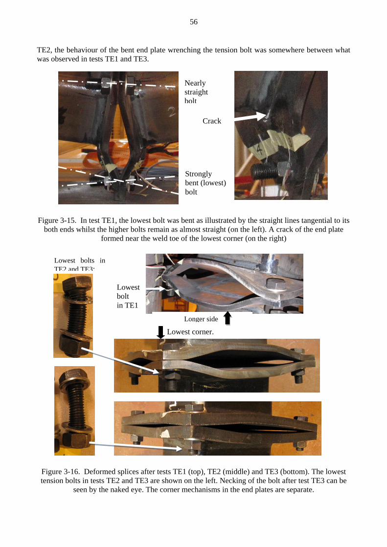
56

TE2, the behaviour of the bent end plate wrenching the tension bolt was somewhere between what

was observed in tests TE1 and TE3.

Figure 3-15. In test TE1, the lowest bolt was bent as illustrated by the straight lines tangential to its

both ends whilst the higher bolts remain as almost straight (on the left). A crack of the end plate

formed near the weld toe of the lowest corner (on the right)

Figure 3-16. Deformed splices after tests TE1 (top), TE2 (middle) and TE3 (bottom). The lowest

tension bolts in tests TE2 and TE3 are shown on the left. Necking of the bolt after test TE3 can be

seen by the naked eye. The corner mechanisms in the end plates are separate.

Crack

Strongly

bent (lowest)

bolt

Nearly

straight

bolt

Lowest corner.

Lowest

bolt

in TE1

Longer side

Lowest bolts in

TE2 and TE3:

57

Next, the weak axis tests TE7 and TE8 representing, respectively, splices S1 (10 mm end plate) and

S3 (20 mm end plate) are compared with each other. The higher initial stiffness and resistance was

observed in test TE8 with the thicker end plate. Oppositely, splice S1 had clearly better ductility

than splice S3, when judged by the maximum rotation in failure.

TE7/splice S1. In test TE7, the yielding of the strongly bent end plates was the obvious reason for

the gradual decrease of the stiffness leading to the collapse. No necking was observed after the test.

Analogy with the failure mode 1 of the T-stub, representing the complete yielding of the flange, was

evident. Separate yield line patterns were indentified in the end plates at the corners (related to the

tension bolts), similarly as observed in test TE1 representing also splice S1. In this mind, the failure

modes were similar whether the weak axis or biaxial test for splice S1 was considered.

At the end of test TE7 (load-controlled part), a loud bang was heard. The sound was obviously

caused by the cracking of the end plate near the weld toe at the corner of the tube. Three more

bangs were heard during the displacement controlled part of the loading. When the entire test was

over, including the additional part, four similar cracks could be seen in the end plates near the lower

corners of the tube. Two of these cracks are shown in Figure 3-17 on the left. In spite of the cracks

in the end plates near the lowest corners of the tube at the edges of the weld toe, the splice could

carry a substantially large load during the displacement-controlled loading (see Figure 3-12).

Obviously, the cracks in the end plate overturned the influence of the strain hardening in the

response of the yielding end plate in bending (and shear) such that a larger load than that obtained at

the end of the load-controlled test TE7 was not seen in the displacement-controlled loading. It is

remarked that the cracks in the end plates of splice S1 i in tests TE7 resemble those appeared in the

lowest corner in test TE1 (Figures 3-14 and 3-15).

TE8/splice S3. In test TE8, the yielding bolt(s) came up in addition to that of the yielding end

plates. Necking of both tension bolts was evident, as shown in Figure 3-17 above on the right. It is

noted that the propagating necking can be related to the instable bolt response. However, test TE8

was terminated when the response of the whole specimen was still increasing even though very

slowly. This can be explained by the decreasing prying action discussed in Appendix A4 based on

FE simulations. In the photograph of Figure 3-17 (on the right), the permanent deformations at the

moment of interruption of the test were seen. They show the plastic deformation in the end plate

and the evidence for the locally instable bolts present in the globally stable specimen. It shoud be

noted that the similar reasoning holds also in the case of biaxial tests TE3 on splice S3.

In addition to the permanent deformations of the end plates, necking in the tension bolts were

accomplice for the decreasing stiffness of splice S3. Thus, failure mode 2 of EC3 was relevant in

test TE8, as it was in test TE3 representing the same splice. The deformed shape of the end plate in

test TE8 can be seen in Figure 3-17 below on the right. Separate yield patterns could be identified

for each corner of the end plate related to the tension bolt, similarly to the biaxial test TE3 on the

same splice: yield line in the end plate near the tube corner took place, while yielding near the bolts

was lacking. It is likely the case that the tension bolts would have broken if test TE8 had been

continued any longer. Bolt fracture would then have been understood as the final reason for failure

of the splice. This would have been most probable also in the case of test TE3.

58

Figure 3-17. The different failure modes in tests TE7 (mode 1) and TE8 (mode 2) can be identified

clearly in the photos representing the tension side of the splice.

TE11/splice S4. Test TE11 was arranged for splice S4 with mid-side bolts, whereas the other tests

on tube splices were arranged with the corner bolts. The same 10 mm plate was used in splice S4 as

in splice S1. Thus, the only difference between them is the bolt placement. Based on the

comparison between the - curves of Figure 3-14, the better efficiency of mid-side bolts in

respect to both the initial stiffness and resistance can be seen immediately as discussed above. In

any case, we next attempt to identify the failure modes present in tests TE11.

Test TE11 was interrupted when the force-displacement curve became almost horizontal. At that

moment, the load of the jack was 302 kN ( = 75.5 kNm). The butterfly shape of the deformed end

plate and cracks in the end plate are shown in the photographs of Figure 3-18 taken after failure.

The plastic deformations of the bent end plates were the primary reason for the gradually decreasing

stiffness followed by the cracks, which appeared at the stage of the almost horizontal response when

plastic deformations grew rapidly. The cracks formed in the lower longer sides of both end plates

near the weld toes and they were directed perpendicularly inside to the end plate (lower photograph

of Figure 3-18). Except for bending of the end plate, the shear likely participated in the forming of

these cracks in the relatively thin end plate used in the splice. Thus, the actual failure mode

resembles (shear) punching of the tube through the end plate but it is related to the tensile parts of

the tube. Whilst yielding and cracks in the end plate were apparent, necking of the lowest bolt was

not that. However, the bolt force must have been quite high in the lowest bolt, which kept the end

plates together during the whole test. Anyway, the failure mode corresponded the mode 1 of T-stub,

characterised as complete yielding of the flange. The yielding of the end plate occurred through the

separate yield line patterns related to the associated tension bolts.

cracks

End plates deformed largely in tests TE7.

This photograph and more when the test

was continued under displacement

control. The separate corner mechanisms

can be identified in the end plates. The

cracks formed in the strongly bent end

plate near the tube corners in the tension

zone.

Lowest bolts with visible necking (above) and

moderately deformed end plates (below) after

test TE8. The separate corner mechanisms

can be identified in the end plates.

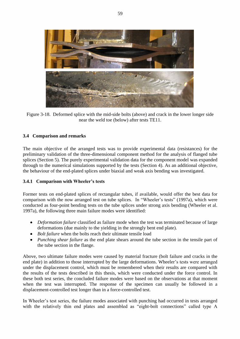
59

Figure 3-18. Deformed splice with the mid-side bolts (above) and crack in the lower longer side

near the weld toe (below) after tests TE11.

3.4 Comparison and remarks

The main objective of the arranged tests was to provide experimental data (resistances) for the

preliminary validation of the three-dimensional component method for the analysis of flanged tube

splices (Section 5). The purely experimental validation data for the component model was expanded

through to the numerical simulations supported by the tests (Section 4). As an additional objective,

the behaviour of the end-plated splices under biaxial and weak axis bending was investigated.

3.4.1 Comparison with Wheeler’s tests

Former tests on end-plated splices of rectangular tubes, if available, would offer the best data for

comparison with the now arranged test on tube splices. In “Wheeler’s tests” (1997a), which were

conducted as four-point bending tests on the tube splices under strong axis bending (Wheeler et al.

1997a), the following three main failure modes were identified:

Deformation failure classified as failure mode when the test was terminated because of large

deformations (due mainly to the yielding in the strongly bent end plate).

Bolt failure when the bolts reach their ultimate tensile load

Punching shear failure as the end plate shears around the tube section in the tensile part of

the tube section in the flange.

Above, two ultimate failure modes were caused by material fracture (bolt failure and cracks in the

end plate) in addition to those interrupted by the large deformations. Wheeler’s tests were arranged

under the displacement control, which must be remembered when their results are compared with

the results of the tests described in this thesis, which were conducted under the force control. In

these both test series, the concluded failure modes were based on the observations at that moment

when the test was interrupted. The response of the specimen can usually be followed in a

displacement-controlled test longer than in a force-controlled test.

In Wheeler’s test series, the failure modes associated with punching had occurred in tests arranged

with the relatively thin end plates and assembled as “eight-bolt connections” called type A

60

connections. In those tests, the connection was quite stiff, and the role of shear in respect to bending

of the end plate was larger than in the other test of the series. Another group of Wheeler’s tests was

carried out with “four-bolt connections” (type B), where either the corner bolts or bolts placed just

at the border of the corner area were used. The character of the type B connection was more

flexible, and the failure mode was either the deformation mode (with excessive yielding of the

strongly bent end plate) or bolt failure. No punching failures occurred for type B connections in the

behaviour of which the role of shear in respect to bending of the end plate was smaller. In tests of

type B connections, either the ultimate failure mode associated with bolts or the excessive

deformation of the end plates took place. It should be noted that failure of the bolts threads occurred

in some Wheeler’s tests on type B connections. The tests on type B connections comprise a series of

strong axis bending tests for the tube splices, which resembles most the tests with corner bolts

(splices S1 to S3) described in this thesis in the case of weak axis and biaxial bending.

In tests TE1 and TE7 with the thinnest end plate (10 mm) and corner bolts, the large deformations

caused by the yielding of the end plate resembled those in which the deformation failure was

observed by Wheeler. The difference is that the cracking of the end plates was observed at the end

of the loading in tests TE1 and TE7 (when the stage of almost horizontal response was obtained),

whereas in Wheeler’s tests, fracture of the bolt was the common reason for failure. It should be

noted that Wheeler did not report on cracks of the strongly bent end plates in type B connections.

Moreover, no bolts broke in the now-arranged six tests, even though the onset of necking was

occurred already in tests TE2 with intermediate end plate thickness (15 mm) and the advanced

necking was observed in tests TE3 and TE8 with the thickest end plate (20 mm). If the force-

controlled loading procedure had been replaced by the displacement-controlled one, bolt fracture

(or other decisive failure mode) of the splice could have been appeared very probably in these tests.

Test TE11 with thinnest end plate (10 mm) and mid-side bolts was the closest to Wheeler’s tests of

type A connections with (relatively) stiffer end plates. The mid-side bolt worked more efficiently in

test TE11, such that the role of shear in the end plate was increased. In tests TE11 with thinnest end

plate (10 mm) and mid-side bolts, the punching shear failure was possibly the primary reason for

the material fracture in the end plate instead of bending. The role of shear in the formation of

cracking in tests TE7 and TE8 is difficult to estimate.

The results obtained in the Wheeler’s test can be seen to be well in compliance with those given by

biaxial and weak axis tests described in this thesis in spite of the different controlling methods used.

Especially, the influence of the end plate thickness could be observed similarly in both series: the

thinner is the end plate, the larger role it has in the splice response.

3.4.2 Remarks

It is emphasised that in all the arranged tests, the gradually decreasing stiffness of the specimen was

caused mainly by the propagating plastic deformations (in the end plate or in the bolts) resulting in

the almost horizontal response before the first cracks appeared in the specimen. Based on this

common character, the arranged tests can be seen as a unified group.

The analogy, which can be identified between the failure modes of the splice flange and the plastic

failure modes of the elementary T-stub (Figure 2-4), must be understood as a prerequisite for the

utilization of the plasticity theory in the modelling of the end-plated tube. For example, the yield

line patterns suggested for the end plate corner with symmetrically placed bolt in Section 5, are

defined such that their failure modes and resistances correspond those of the equivalent T-stub,

which replaces the actual component.

61

The separate yield line patterns were observed in all splice tests with four-bolt layout whether the

tests were biaxial or weak axis bending tests or whether the corner or mid-side bolts were used.

These patterns have no common yield lines with the other patterns in the splice such that no

grouped bolt mechanism occurred in the tested splices. It can be suggested that these patterns

appear independently of the direction of the (resultant) bending moment. This assumption is

convenient, especially, when the component models are formed for the splices under arbitrary

biaxial bending and, in addition, it is in compliance with the philosophy of the component method.

Simple yield line patterns, which will be assumed for the component analysis of the considered end-

plated splices, are suggested in Section 5.

It is reminded yet that the separate splice tests on biaxial bending cannot be found in the literature.

The three-point bending tests were used instead of the four-point tests in order to avoid constrains

against the transverse movements of the specimen under biaxial bending. A successful biaxial test

provides that the inclination of the hydraulic jack remains as sufficiently small during the test. The

possible shear forces at the splice can be shown to be carried by friction between the end plates,

such that the bending response of the splice is in the main role. A simple manipulation of the

directly measured results is required in order to determine the flexural behaviour of a considered

splice.

62

4 NUMERICAL ANALYSIS OF THE TUBE SPLICES

4.1 Introduction

In the numerical part of this study, the responses of the tube splices are simulated through the three-

dimensional finite element analysis (3D FEA). The numerical model is needed to produce the

enlarged validation data supported by the tests for the 3D component method. Accordingly, the

principal objective is to determine the resistances of the splices against biaxial bending in the

arbitrary direction. The validity of the numerical model itself is investigated through the

comparisons between the predicted responses and those measured in the tests. The complementary

FE simulations on tube splices under axial tension or (pure) biaxial bending are presented in

Appendices A4 to A6.

4.1.1 Special features of the considered splice problems

For the 3D FE analysis of the end-plated splices under biaxial bending, the essential structural

features of the problem must be introduced to the model. In all tests, the end plates deformed

permanently in the tension zone whilst advanced necking of the bolts was seen in the tests with the

thickest end plates (Section 3). No buckling phenomena in the compression zone of the splice were

observed in any of the arranged tests. Accordingly, the elastic-plastic behaviour played the

determinate role in the splice response. In the case of flexible end plates (in respect to the bolts), the

end plates bend strongly in the tension zone such that large rotations were present. The minimum

requirement is that the geometrically nonlinear behaviour related to the “finite rotations” must be

taken into account in the computational model. The strains of 3% to 10% were measured in the

arranged tests on the outer surface of the end plates in the strongly bent areas (Perttola & Heinisuo

2011). Thus, the model must take into account both the finite strains and finite rotations in order to

properly simulate the behaviour of the end plate. In addition, the possible membrane action and

influence of shear on the response of the bent end plate can then be described. The large strain

values in the end plate indicate not just the geometrically nonlinear aspect of the problem, but also

the need for the constitutive modelling, where the relation between the finite strains and the related

stresses is defined. It should be noted that in the tensile tests, these stress and strain quantities are

called “true” in order to make a difference between the nominal (engineering) and actual values.

The necking phenomenon of the tension bolts was observed in some tests (TE3, TE8) such that the

very large strains had been present in the associated bolts. The maximum tensile force in a bolt is

reached with the onset of necking when the decrease of the cross-sectional area cannot be

compensated by the strain hardening. The large strain values due to the advanced necking require

the modelling of the stress-strain curve far beyond the limit related to the onset of necking in the

tension test. It is emphasized that necking cannot be simulated realistically without the full

nonlinear formulation of the kinematics and actual description of the stress strain curves. Necking is

influenced by bending of the bolt, which is investigated through the simulations of the splices under

bending in Appendix A6. If the other parts of the splice are able to substitute the decreasing bolt

force due to necking, the splice is able to carry more load as a whole. This phenomenon is related to

the decreasing prying of the bolts, which has been discussed in Appendices A4 and A6 in the case

of the splice in axial tension and splice under bending, respectively. The used stress-strain models

for the end plates and bolts are discussed in Appendix A2 as defined consistently with the known

material parameters. These uniaxial curves were generalized into 3D FE analysis through the

principles presented in Appendix A1. In Appendix A1, also the basics of the von Mises type of

classical plasticity model accompanied with the strain hardening description was discussed.

63

For the analyses of the bolted joints, contacts have to be modelled. The used model must be able to

describe the essential changes in the contact stresses and contact areas. Contacts between the end

plates will be in the key role in the analyses of the end plated tube splices under bending (or in

tension). In the compression zone, the compression resultant must be transferred through these

contacts. In the tension zone, contacts between the end plates may appear because of prying of the

bolt. In the prying action, the end plates push against each other in order to equilibrate the

additional tension force in the bolt due to prying. The contact stresses and contact area between the

end plates may change because of the external loading or because of bolt pre-tensioning, which is

demonstrated in Appendix A4. In any case, the contact force, the separation of the contacted

surfaces (opening) and the occurrences of the new contacts (closing) should be described when the

interaction between the end plates is simulated numerically. The tight contacts without any relative

movements between the washers and end plates were observed in the arranged tests. Obviously, the

contacts between the end plates and washers as well as the internal contacts in the fasteners do not

change essentially due to the external loading after the pretension of the bolts in the splice under

bending. The interaction between the end plates was modelled as normal contact between the two

deformable and impenetrable bodies (Appendix A3) whilst contacts related to the fastenings are

assumed to stay closed during the external loading (Section 4.4.2).

In principle, the actual initial state involving loading, geometry, boundary conditions, contacts,

stresses and strains in a structural problem should be introduced to the computational model at the

beginning of the analysis. In practise, the initial state has to be presented as idealised (or as

nominal) for numerical simulations, because the small deviations from the “nominal state” called

initial imperfections are usually not known. If the studied feature in the response of a structure has

no special tendency to be affected by the initial imperfections, these imperfection can be neglected

in the model. It should be noted that the initial imperfections are very probably distributed in a way,

which deviates from the prevailing structural symmetry. On the other hand, if the initial

imperfections have no essential influence on the studied feature in the structural behaviour, it is

immaterial whether these imperfections are distributed in a symmetrical or asymmetrical way.

When the studied splices under bending are concerned, the buckling phenomena are not relevant

and the resistance is essentially obtained as the plastic limit load in which case the initial

imperfections only play the secondary role. In the case of the end plated splices, welding between

the beam (tube) and end plate may cause changes in the straightness of the end plates, which affect

contacts between the end plates in the initial state and the developing prying action. This may have

an essential influence, for example, on the overall response of the splice but not on the ultimate

plastic resistance. It has been observed (Wheeler 1998; Wheeler et al, 2000, Willibald 2003) that the

initial stiffness (or overall response) of a tube splice can be simulated quite nicely by the idealised

model in the case of the thin end plates (flexible in respect to the bolts) whilst, the stiffness

predictions are poor for splices with thick end plates (stiff in respect to the bolts). The latter one was

explained as a consequence of the deficient description of the initial imperfections (strains) related

especially to welding. Wheeler et al (2000) studied the influence of the initial strains on the

response of the end plated splice by introducing a typical deviated shape to the end plate caused by

welding. This demonstration showed that although the overall response of the splice was dependent

on the given deviation, the resistance was not. When the strict description of the initial state has

only a secondary influence on the splice response at the large load level, i.e., on the splice

resistance, the simplified modelling of the initial state can be seen as reasonable in the context of

the main objectives of this thesis. Based on reasoning of this kind, the “idealised initial state” is

introduced to those models used in the FE simulations in this study. For the more accurate

modelling, a preceding analysis of successive events simulating the fabrication of the splice would

be desirable. This is, however, outside the scope of this thesis.

64

In the 3D FE simulations, the equilibrium path is followed in the case of the splice under bending

moment or in axial tension. In the solved path, the equilibrium should prevail, the deformations

have to be kinematically admissible and the constitutive laws must be fulfilled. The geometrically

and materially nonlinear features are inevitably present in the solution of the splice problem

including contact behaviour. Bursi & Jaspart (1997a, 1997b, 1998) have profoundly discussed the

physical character of the analysis of the end plated connections. They claim the importance of the

description of the actual material behaviour including strain hardening. They also pay a special

attention to the bolt models such that the response of a (tension) bolt can be described through a

computationally efficient way calibrated against the advanced numerical analysis results. According

to the examples in the literature (Bursi & Jaspart 1997a, 1997b, 1998; Wheeler 1998; Wheeler et al,

2000, Willibald 2003), the structural symmetry can be exploited in the FE analyses of the end plated

connections, which is computationally efficient. It should be emphasized that although the elastic-

ideally plastic model could reveal the right level of the knee point between the elastic and plastic

stages of the response, it would be insufficient when the actual response of the considered splices is

traced after the knee point. The elastic-ideally plastic model ignores the strain hardening, which is

in the decisive role when the behaviour of the strongly bent end plates is simulated. In addition, the

ideally plastic model fails to describe necking of the bolts, which play the determinate role in the

splices with thick end plates. The response described after knee-point of the splice without proper

description of strain hardening and necking of the bolts is nonsense. In this context, it is not

reasonable to use elastic-ideally plastic model in the nonlinear numerical analysis of steel structures.

4.1.2 Elastic-plastic model

In this work, the splice behaviour is described through the elastic-plastic model, such that the main

objective is to simulate the splice response to the increased loading and, furthermore, determine the

resistance of the considered splices supported by the tests. A decisive difference between the actual

material response and the used elastic-plastic model is in the missing ability of the latter to describe

the material fracture. However, the propagating plasticity in the end plates and in the bolts can be

seen as the main cause for the gradually decreasing stiffness of the splice. The cracks appeared in

the end plates and possibly affected the response of the splice only in tests with the thinnest end

plates just before the end of the tests (test TE1, TE7 and TE11). No bolt failure was seen in any

arranged test though it was expected to appear in the tests with the thickest end plates (TE3, TE8).

In elastic-plastic type of structural response, the elastic properties prevail at the beginning, whilst

the plastic flow takes place gradually and finally has the decisive role. In principle, a knee point can

be identified between the stage of the elastic response and the stage, where the propagating

plasticity prevails the structural response (typically in the strain hardening stage). Finally, the

plastic limit load defines the load-carrying capacity of the structure. After the limit point, the

descending stage follows in the response. A prerequisite for the unambiguous solution of the

nonlinear elastic-plastic problem is the strain hardening material with the associative flow rule

sometimes called “standard material with hardening property” (Lubliner 1990). As long as no

unloading occurs, there is no distinction between solutions for nonlinear elastic and work hardening

plastic material, because the incremental uniqueness implies the total uniqueness of the stress and

strain fields. Without unloading, any state of the corresponding loading can be solved by successive

(quasi) elastic steps. Formally, the positive definiteness of the elastic modulus in the tangential type

of relation (Eq. (A1-1) in Appendix A1) between the infinitesimal stress and strain components is

required. The uniqueness of the solution for the elastic-plastic problem is discussed in Appendix

A1. It should be noted that all used material models in the analyses of the splices are positive

definite.

65

The elastic-plastic material behaviour of the splice parts is described such that the plastic part was

modelled according to the -plasticity (von Mises). The plastic models are equipped with the strain

hardening property. The knowledge of the material behaviour is based on the one-dimensional

information (tensile tests). Consequently, the three-dimensional material model must be obtained

through the generalisation of the one-dimensional data obtained by the tensile tests. The constitutive

properties of the parts of the splice were known through the material certificates. The material tests

arranged for the delivery lot by the manufacturer are reliable, but they only offer discrete type of

information about the material response instead of the whole stress-strain curves. This data usually

includes the yield strength ( or ), ultimate strength ( ) and ultimate stain value at fracture

( ). The aim is to utilise this discrete type of data and to first construct the one-dimensional stress-

strain curves. The missing data are completed in accordance with the results of the SINTAP project

(Structural INTegrity Assessment Procedures for European industry described in the papers

(Bannister and Trail 1996; Bannister 1998; Bannister et al. 2000). For stress-strain curves without

the sharp yield stress, the formulas of the classical Ramberg-Osgood model are exploited. The R-O

model represents a power law type of formulation. In the case of discontinuous yielding, the three

segments including elastic part, plateau and hardening stage of the stress-strain curve are described

separately. The uniqueness of the elastic-plastic solutions, the concepts behind the plastic material

model and generalization of the one-dimensional model into 3D are discussed in Appendix A1. In

Appendix A2, the one-dimensional stress-strain curves of the splice parts used in the accomplished

FE analyses are presented.

It should be noted that the data of steel certificates is normally given for the base material. The

fabrication of the tested structure may change these properties, for example, due to the cold forming

and welding. In principle, the tensile test specimen should be taken from the material exposed to the

cold forming and welding simulating the fabrication. In the case of the considered splices, the

welding between the tube end plate might change the properties of the end plate such that it is

relevant in respect to the accomplished analyses increasing the resistance of the splice. Oppositely,

the welding can decrease the ductility of the end plate (in HAZ), which is taken neither into

account. The influence of these factors on the splice resistance is difficult to judge.

4.1.3 FE analyses by ABAQUS

The finite element method was used in the elastic-plastic analyses of the considered splice

problems. The FE program must be capable of the descriptions of the nonlinear kinematics and

elastic-plastic material behaviour. In addition, the program has to include in methods for the contact

analyses embedded in the problem. These requirements are provided by a well-known FE program,

ABAQUS, which was adopted for the accomplished analyses. The specific version used is

“ABAQUS 10.6”, documented in the corresponding manual (ABAQUS 2010). The nearest versions

of the program, before and after the used version, offer essentially the same tools for the analyses.

Other commercial software packages with sufficient properties are, for example, FE programs

ANSYS and LUSAS. In any case, an advanced finite element program like ABAQUS can offer full

nonlinear analysis and involves many ready options, for example, for the bolt pretension. For the

computing, the researcher used a personal computer equipped with a 64-bit Intel processor with a

clock speed of 2.53GHz (Intel (R) Xeon (R) E5630 CPU @2.53GHz). In the accomplished

analyses, the maximum elapsed (wall clock) time for a single run was a little more than two days

when the bending tests were simulated. Longer duration times were not tolerated, and the associated

model was developed within this limit. It is noted that most of the analyses took much shorter times,

and those parts of the analyses related to the post-critical stages of the response took relatively

longer times. No optimization in its real sense was arranged in order to obtain numerical solutions

66

efficiently; in this regard, the numerical modelling was made more intuitively rather than based on

strict comparisons. The verification of the used model is described in Sections 4.3.2 and 4.3.3

An incremental and iterative solution procedure is required when the considered, geometrically and

materially nonlinear splice problems are solved. The contact constrains must be enforced also

through an iterative procedure added to the equilibrium iterations. The converged solutions in the

equilibrium path should be found in spite of the occurrences of the global or local instabilities. A

local instability typical for bolted connections is caused by necking of the tension bolts, which can

be described by combining the nonlinear kinematics and plastic behaviour. The aim is to follow the

equilibrium path of the splice under bending (or in axial tension) over the limit load and continue

this analysis to the stage of the descending response. The model and the used solution procedure

must be chosen such that this objective can be obtained. The solution procedures of the FE

formulations for the nonlinear static problems are discussed in Appendix A7. In this appendix, some

references about the nonlinear FE method and continuum mechanics are given, which may help to

understand the character of the models and solution procedure required in the nonlinear analyses.

Especially, the given literature is needed as support when the ABAQUS manual is interpreted. The

role of the ABAQUS manual is important because the source code of ABAQUS is not public,

which naturally concerns most of the commercial FE programs. In principle, the analyst can define

the model and the related data but the solution itself is determined by a black box, which hopefully

works as explained in the manual. Of course, the benchmarks (e.g., ABAQUS benchmark manual)

can dispel the doubts about the correctness of the FE analyses accomplished.

The modelling errors are always present, because the computational models are more or less

idealised. The judgement of the modelling error belongs to the tasks of validation. Through the

verification, an analyst can convince himself that the approximate solution by the FE model is

obtained correctly. In the case of the complicated, nonlinear problems, the exact solution is not

known. Then the rightness of the solution can be investigated based on the convergence tests. In the

Appendix A9, the convergence tests intended for the stress analyses are described. The similar

procedures are utilised in this study when the mesh density is determined for the used FE models.

4.2 Structural models

Next, the structural models used in analyses of considered splice problems are introduced. These

models include the splice under biaxial bending (type I, Section 2.2.7) and the splice in axial

tension (type II), respectively. The models for splice under biaxial bending represent the three-point

bending tests whilst the model of splice in axial tension is used as an elementary case in the

verification of the FE model for the splice in biaxial bending. The arranged bending tests comprise

the experimental data for the (direct) validation of the numerical model for the type I problem. FE

simulations based both on these types are discussed in Appendices A4 to A6.

4.2.1 Modelling of contacts according to their roles in the splice

Contacts are present and play an essential role in the response of a bolted joint the structural

response of which is not possible without them. The response of the deformed bodies affects their

contacts and vice versa such that the contact areas and the contact forces may vary during the

loading. In the joints under pure bending and tension, the bolts are mainly in tension caused by pre-

tensioning and the external loading of the joint. When the shear and torsional forces are absent,

contacts between the bolt and the edges of the holes in the end plates are missing or have only a

67

minor role. A connection like this is classified as a tension connection, whereas shear connections

and their behaviour are excluded in this context. In tension connection, contacts are inside the

fastener and between the fastener and the end plates such that the forces are transferred through the

bolt force from one end plate to another. In Figure 4-1, possible contacts in the tension connections

are demonstrated by considering a separate fastening comprising a screw (bolt), nut and washers

attaching two end plates together. In this case, contacts may arise:

between the end plates (A),

between the parts of the fastener including a bolt, nut and washers (B and C), or

between the fasteners and end plates (D and E).

In the initial state of the splice, the surfaces potentially in contact may be connected without a gap

or separated with a nonzero gap. Typically in pre-tensioning, the gaps between the parts of the

fastener are closed, and the associated contacts between the connected parts (end plates) are formed.

During the loading, the surfaces may meet in new contacts, or the formerly contacted surfaces may

separate from each other. The external loading changes the contacts in the joint such that in the

current configuration, contacts represent those required to carry external loads deviating from those

formed initially because of pre-tensioning. In any case, the tension bolt is in axial tension ( )

or almost in axial tension, with bending ( ) playing a secondary role. In the figure, possible

contacts (from A to E), are illustrated by four figures for clarity though all of them may appear in a

single fastening at the same time. In the assembly, the connected plates are clamped together by the

preloading of the bolt. The pretension force must be equilibrated by the clamping force going

through contact A (figure on the left above). If the clamp force has not overcome by the external

loading, the pretension force can keep the connected plates clamped together. If the external loading

causes tension larger than the clamping force, contact A is lost. It should be noted that the prying

action discussed in Appendix A4 makes the situation more complicated. The forces inside the

connector go through “internal contacts” B and C (on the right above). Contact B appears between

the bolt head and washer whilst contact C occurs between the mating treads of the screw and the

nut. The bolt force must be equilibrated by the force going through contact D between the washer

and the end plate (on the left below). Contact E between the bolt and edges of the holes (on the right

below) arises only when the bolt is sufficiently bent. Contact E is more probable in joints with

relatively flexible end plates, such that the bolt is enforced to bend with the strongly bent end plates.

In this thesis, the considered fastenings act in an end-plated tube splice under bending in the tension

zone (or in splice in axial tension). Contacts are modelled for the finite element analysis of the

splices according to next assumptions. In the assembly, the bolts are tightened to the intended pre-

tensions. Accordingly, the pretension forces cause contacts (A to D of Figure 4-1) at the first stage,

which is understood as the initial state for the splice problem under external, monotonically

increasing loading. In a splice under bending, the compressive resultant force is transferred through

contacts between the end plates (A) the changes of which must be described when the response of

the splice is simulated numerically in an essentially right way. A bolt in the compression zone keeps

that bolt force, which it has obtained through pre-tensioning and no essential changes in contacts B

to D are expected in respect to both contact areas and forces. In the tension zone of the splice under

bending or in the splice in axial tension, the bolt force may change significantly due to the external

loading although contacts (contact areas) inside the fastener (B and C) and, moreover, between the

fastener and end plates (D) remain as without separations. This presumption was confirmed by the

arranged tests in which no gaps were observed in these contacts during the tests (Section 3). Thus,

only the forces transferred through internal contacts B to C and contact D between the washer and

end plate are expected to change such that the fastener can be modelled as monolithic and the

contacts between the washers and end plates correspondingly without relative movements between

the contacted surfaces. In the tension zone, the additional bolt forces caused by the prying actions

68

are equilibrated by the contact forces between the end plates. Obviously, contact (A), which is due

to the bent end plates of the splice pushing each other in the tension zone, requires description of

the varying contact area and force. Altogether, the plausible modelling of contacts between the end

plates must be able to take into account the changes in both contact area and force, whereas those

contacts in the pre-tensioned fasteners can assumingly be analysed through the simplified

modelling. Finally, it should be noted that in the FE simulations on the considered splices under

bending (or in tension), no contacts of type E occurred.

At some stage in the splice response against axial tension, the prying force (in the bolt) attains its

maximum value and starts to decrease when contacts between the end plates disappear. The role of

the prying effect changes as opposite such that the decreasing prying effect compensates to some

extent the weakening of the bolt after the onset of necking. An occurrence of this kind is described

in Appendix A4 through FE simulations for splice S1 in axial tension. This phenomenon, which can

be characterised as the reverse prying action (or relaxing prying), happens also in the tension zone

of the splice under bending as explained in Appendix A6.

Figure 4-1. Contacts A to E in a tension connection: between the clamped plates (A), internal

contacts of the fastener (B and C), between the washer and end plate (D) and between the bolt

shank and hole (E).

Contact analysis is usually computationally expensive, whereas savings obtained by the simplified

contact analysis methods can be considerable. This is particularly relevant in three-dimensional

analyses, which need plenty of computer capacity and thus make it reasonable to avoid the

complicated contact models. Of course, the aims of the analyses have an effect on the needed

particularity of the contact modelling. For example, there may be no need to model the local

phenomena, including contacts, accurately if they do not have a particular influence on the global

response in interest. In the analysis of the splices, the interaction between the end plates (A of

Figure 4-1) represents contacts with such an “essential influence”. This concerns both contacts in

the compression zone and those transmitting the prying forces in the tension zone. Contacts of types

B, C and D obviously play the secondary role in the global response. If contacts of type E were to

appear, they should be taken into account in the analysis.

69

4.2.2 Simplified bolt geometry

The fastening (bolt, nut and washers) is modelled as symmetric such that the symmetric boundary

conditions can be defined on the internal surface of the bolts, which coincides with the transverse

symmetry plane in the considered splice problem (Figures 4-4 and 4-8). Moreover, the pretension

forces of the bolts satisfy the requirements for the structurally symmetric loading. In the

computational model, the intended (pre)tension force can be introduced by cutting off the related

length from the bolt. A procedure for pretension like this was readily available in the used version

of Abaqus (v. 10.6). The slight pretension can also be utilised as a preceding step in order to

establish the contacts for the subsequent analysis of the splice. Then the next loading step is

required for the regular preloading of the bolts. A simplified bolt model is introduced below.

The simplified bolt model is defined such that the bolt, nut and washers are presented as a

monolithic connector. This is based on the assumption that, in the pre-tensioned fastening, the parts

of the fastener (bolt, nut and washers) are in tight contact during the loading. The threaded part of

the bolt is replaced by a round bar, which is reasonable in the static analysis. The necking

phenomenon can still be described through the elastic-plastic analysis in a reliable way (Section

4.4.3). The suggested geometries are shown in Figure 4-2 as two versions, B1 and B2. The latter

was used in the analyses of the splice problems. Version B1 was used only in the separate analyses

of bolts (in which case there is no difference between these versions). The tensile stress area of the

full threaded grade M20 bolt ( = 245 mm2) replaces the cross-sectional area of the shank.

The corresponding radius rs then has a value of 8.33 mm. The total free length ( ) of

the shank consists of the thicknesses of the connected end plates ( ) and the washers ( = 6

mm). In order to obtain symmetry, a similar idealised head is used at both ends of the simplified

bolt model with the height of 17.25 mm, which is based on the average of the heights of

the bolt head and nut . The inner diameter of the washer was denoted by mm in the

figure. In version B1 of the bolt geometry, the washer and bolt head have the same outer diameter

as the washer (D = 36 mm) up to the end of the head. In version B2, a different diameter is used for

the bolt head or nut (Dh = 30 mm corresponding to the minimum diameter of the hexagonal M20

head). It should be noted that, because of the shaping of the bolt head (or nut), the possible contact

area between the bolt head (or nut) and the washer is round (not hexagonal).

Figure 4-2. Simplified models B1 and B2 for the bolt assembly.

70

4.2.3 Structural symmetry

Structural symmetry prevails when the shape, material properties, supports and loading of the

structure are symmetric with respect to a plane. Then, the response of the whole structure can be

obtained by reflecting the partial solution through the associate plane to the symmetric part of the

structure. The symmetric boundary conditions can be defined on the internal surface, which

coincide in the symmetry plane. The interaction between the surfaces, which initially are symmetric

in respect to the symmetry plane, should be defined consistently with the symmetry requirement.

The achievable benefit from structural symmetry depends, essentially, on the number of the

reflective planes. The structural symmetry can also be utilised with the nonlinear problems although

the superposition is no longer available for the solution. The fundamental requirement is that the

symmetry must prevail not only in the initial state of the structure but also during the loading.

Moreover, the points, which can be reflected to each other, should face the similar stress-strain

histories.

In the FE analyses of the considered splice problems, structural symmetry can be exploited. The

size of the computational models can be reduced significantly despite the asymmetric behaviour

typical of the connections by bolts. The three-point bending tests, which are used as the driving

examples of the thesis, are modelled as symmetric in respect to the transverse vertical plane at mid

span (Figure 4-8). The bolts must then be described also as symmetric, which had been taken into

account when the simplified bolt model was introduced in Section 4.2.2. As a consequence of the

one (transverse) symmetry plane, the analysis of other half of the structure is sufficient (1/2-model).

In the case of the splice under axial tension, the structural symmetry prevails in respect with three

orthogonal planes the two of which are longitudinal. Then the solution for the 1/8-model suffices,

which requires the double symmetry of the splice. The axial normal force (on the left in Figure 4-

3) and the response caused by it can be seen as symmetric in respect with two longitudinal

symmetry planes, which divide the splice into four identically behaving parts. In the figure on the

right, three loading cases for the splice under (pure) bending are shown. In strong axis bending

( ) and weak axis bending ( ), there is one longitudinal plane of structural

symmetry in both (the 1/4 model would be the sufficient). In the case of biaxial bending (

shown on the far right of the figure, there are no longitudinal reflecting planes. Thus, only

the transverse symmetry plane can be utilised as the reflecting one in the analysis of the splice

problem under arbitrary biaxial bending.

Figure 4-3. Longitudinal symmetry planes in problems of type I and II.

In practical situations, there cannot be structural symmetry in a strict sense because of the initial

imperfections. The imperfections and the related deviations from the symmetry are usually not

known. However, the influence of the initial imperfections on the studied feature of the structural

71

response might remain as small provided that this feature in question has no special sensitivity to

these imperfections. For example, the sensitivity of the plastic resistance to the initial imperfections

is typically low, when the resistance can be determined as the plastic limit load, but high when the

buckling is concerned. The considered splices have no deformable parts (key components) the

resistance of which are critical due to the buckling. The deformations in the tension zone play the

decisive role in the considered splices whilst the parts in the compression zone remain less active.

Many comparisons between the numerical results exploiting the structural symmetry and the tests

results (Bursi and Jaspart 1997a, 1997b, 1998; Wheeler 1998; Wheeler et al, 2000, Willibald 2003)

show that the resistance of the end plated connections is not sensitive to initial imperfections. Of

course, the buckling have no role in any of these cases.

4.2.4 Structural model for splice in axial tension

In the problem of type II, a tube splice in axial tension shown in Figure 4-4 is considered. Three

symmetry planes can be utilised: the transverse plane, which divides the structure into two

partitions at mid span, and two longitudinal symmetry planes of the tube and its splice cross-

sections, as shown in Figure 4-4 (below). Thus, it is sufficient to analyse only one eighth of the

structure (1/8-model) presented in Figure 4-5. The loading scheme of the computational procedure

will be conducted under displacement control in order to follow the equilibrium path over the limit

point. Then the tube including the splice is pulled from its ends such that the total elongation of the

structure equals (Figure 4-4), which replaces loading arranged by evenly distributed normal

stress . The axial normal force can be obtained from the results of the displacement

controlled analysis by the integral defined over the tube cross-section such that

represents a solution for the certain value of the controlled displacement , which is

increased incrementally (i.e., step by step) in the computational procedure.

Figure 4-4. Structural model for splice und axial tension (Abaqus/CAE).

The symmetric boundary conditions on the internal surfaces of the structure, coinciding with ,

and coordinate planes in compliance with Figures 4-5 and 4-6, are

BCxy: (4-1a)

BCyz: (4-1b)

72

BCzx: (4-1c)

where the subscripts x, y and z refer, respectively, to the rectangular coordinate axes, with whose

direction the displacements coincide, or about which the rotations are

defined. The internal surfaces on which the symmetrical boundary conditions marked BCxy are set

in the splice problems are the bolt cross-sections at the mid span. Consistently, the bolts must be

described as symmetric in respect to the plane. At the transverse symmetry plane, the internal

surface is constrained against perpendicular movement and the rotations about any line

coinciding with the associated plane are not allowed ( ) according to the Eq. (4-1a). In

short, the plane where the symmetric boundary conditions are given remains a plane whilst the

transverse displacements in the direction of the plane of symmetry and the rotations about its

normal vector are permitted. The boundary conditions (4-1b) and (4-1c) are defined in the internal

surfaces of the end plates and tube, which coincide in the longitudinal symmetry planes. The

internal surfaces, where the boundary conditions are defined, are shown in Figure 4-6.

Figure 4-5. One eighth of the structure (Abaqus/CAE).

Figure 4-6 Internal surfaces for the symmetric boundary conditions (Abaqus/CAE)

Contacts arising between the end plates of the splice were replaced by frictionless normal contact

(see Appendix A3) between the end plate of the reduced model and the rigid surface associated with

the transverse symmetry plane of the model. The end plate of the splice is allowed to separate from

the rigid surface during the loading opposite to the symmetric boundary conditions determined in

the intersection of the monolithic structure. The rigid surface coinciding in the transverse symmetry

plane must be restrained against any rigid body motion. In the contact analysis, the rigid surface

73

must be selected as the master surface in the contact pair with the deformable end plate The role of

contacts in the response of the bolted splice under axial tension, including prying action, was

investigated by the numerical simulations in Appendix A4.

Because of the assumed frictionless contact between the end plate and the rigid surface, only the

normal tractions can arise. Therefore, the direction of the resultant contact force C must coincide in

the axial direction of the tube. On the other hand, the symmetric boundary conditions for the bolts at

mid span are defined independently; therefore, only the contact force must be equilibrated by the

axial component (reaction force) at the point support used to prevent the rigid body motion of the

rigid plane. This holds wherever the (point) support is placed. Instead of integrating tractions over

the contact area to obtain the resulting contact force, it is simple to determine the value of axial

reaction force . The axial forces and the associated stress distributions acting on the tube

and its splice are demonstrated by the free body diagram of Figure 4-7 on the left. It is emphasised

that the stress distributions shown are only illustrative. Based on the requirement for the equilibrium

of the axial forces, the tensile force per quarter of the tube cross-section must be equal to the bolt

force minus the resulting contact force , or

. (4-2)

Thus, the axial tensile force of the whole tube can be obtained simply for each enforced

displacement when the associated bolt and contact forces are known. Of course, the axial force

could also be integrated over the tube cross-section, which usually is more laborious.

Figure 4-7. Schematic force balance between the resultant forces (Abaqus/CAE).

Averaged axial displacement. The displacement (Figure 4-5) can be divided into the part that is

caused by the elongation of the tube and the part that is related to the deformation of the splice. The

tube deformation can be excluded by computing the splice deformation as the average value of

axial displacement over that tube cross-section in which the tube and the end plate meet each

other. Then it represents an averaged axial displacement of the splice, written formally as

, (4-3)

which is defined analogically with the generalised axial displacement of the tube. Then, the

deformation of the splice is described consistently with the generalised beam theory (Vlasov, 1962;

Schardt, 1989). The latter equality in Eq. (4-3) is justified in the case of the constant wall thickness

when the coordinate s is running along the centre line of the tube wall in the cross-section with the

circumference . In the splice problems considered, the tube remains in the elastic range

whilst the splice yields. The stiffness of the tube in axial tension is, moreover, much larger in

comparison with the stiffness of its splice such that the approximation

74

(4-4)

is acceptable. Then the displacement at the tip of the tube directly represents the axial

displacement of the splice.

4.2.5 Structural model for splice under biaxial bending

The biaxial bending tests arranged on the tube splices were numerically simulated based on the

structural model illustrated by Figure 4-8 on the right. The unwanted inclination angle shown in

the figure on the left was neglected in this consideration. This simplification is reasonable, when the

inclination remains as sufficiently small as happened in all the arranged tests. If this would not be

the case, the hydraulic jack (being supported to the loading frame) should be modelled together with

the specimen, such that the direction of the external load on the deformations of the structure

could be taken into account. Besides the inclination of the load, the unwanted shear force may

appear in the tests at mid pan. However, this shear is taken by the friction between the end plates as

explained above in Section 3.3.1, where the arrangements of the biaxial bending test are described.

It is emphasized that the shear force disappears at the mid span in the idealised model. The normal

force is missing, in turn, because of the freely allowed axial movements at the supports. Thus, the

flexural response of the splice alone is described by the used model (type I).

Figure 4-8. Inclination of the jack is neglected in the used model (drawn in Abaqus/CAE).

The significance of the deviations of the idealised model from the actual test is discussed in respect

with the initial stiffness. At the beginning of the biaxial test, the jack is in the vertical position such

that inclination angle disappears ( ). In principle, the initial stiffness v equals the

derivative at the beginning of the test, when the load , the vertical displacement

and inclination at the same time. From this theoretical point of view, it does not

matter if the small inclination angle is neglected by using the computational model shown in

Figure 4-8 on the right. In practise, the initial stiffness is replaced by the relation

determined for a finite step. Because

, it holds that provided that inclination angle ( is small

enough. It should be noted that the used upper limit for the associated step was between 10 and 40

kN (Table 3-12) such that the corresponding inclination was less than in every arranged biaxial

test (Perttola & Heinisuo 2012).

75

Biaxial bending appears in a specimen under vertical load V when the rotated position of the

specimen about the longitudinal axis is deviated from that causing strong (or weak) axis bending.

Then, both the weak axis component and the strong axis component appear correspondingly

such that they cause, respectively, the associated bending deformations (must be solved

incrementally at the same time). In practise, asymmetric bending prevails causing the nonzero

horizontal movement ( ). It should be noted that the inclination angle, which was the largest at

the end of the test, was always smaller than in every arranged test (Section 3). Small inclination

like this has no essential influence on the bending resistance of the splice, which can be justified by

the next theoretical reasoning based on plasticity theory. The (plastic) resistance for resultant

bending moment is defined as distance from the origin to the failure curve around the origin in the

- plane such that the direction of the resultant moment is tangential to this continuous and

convex-shaped interaction curve. Then the small change in the direction of the resultant moment

does not change the value of the resistance much because the distance from the origin remains

approximately as the same. Altogether, both the stiffness and resistance of the splice can be

determined through the computational model with the vertical load provided that the inclination

angle remains small enough in the actual test.

The specimen in the biaxial tests was equipped with the loading shelf as an additional part of the

splice. The loading shelf is, however, in the compressive zone of the splice under bending and,

therefore, their influence on the splice behaviour is assumed to be negligible. This was verified by

comparing the numerical analysis results on the splice response with and without the loading shelf

(Section 4.4.2). Therefore, these extra parts of the end plate are unnecessary features and thus could

be removed from the structural model.

1/2-model. Reflecting symmetry is employed in respect to the transverse plane at mid span. The

coordinate axes are defined as shown below on the far right of Figure 4-9. The -axis coincides with

the longitudinal direction, whilst the - and -axes represent, respectively lateral and vertical

directions in the transverse plane. In order to construct a reduced model, the transverse symmetry

plane is replaced by a rigid surface, which is restrained against rigid body motion. In the 1/2-model,

contacts between the end plate and the rigid surface are described by the frictionless normal contact

(Appendix A3) analogically with the splice in tension. The symmetric boundary conditions are

given to the bolts in the internal surface coinciding in the symmetry plane at mid span in

compliance with Eq. (4-1a). The bolts can move in the symmetry plane.

No gaps or forces were introduced between the end plate and the rigid surface in the initial state,

which corresponds to an assumption of the idealised (nominal) geometry. After the onset of the

external loading, the end plates may be either in contact or separated from each other. The 1/2-

model (or 1/8-model) forms a mechanism unless contacts between the end plate and the rigid

surface can offer the necessary support for the model. Therefore, a preceding step preceding the

onset of the external loading or the pretension of the bolts is needed in order to ensure the

successful start to the analysis. In the preceding step, thus, a small movement is introduced to the

splice to establish contacts in order to avoid a mechanism. The first actual step can be taken also as

the small pretension of the bolts during which contacts are formed. After pretension, the “regular

steps” follows.

In Figure 4-9 (far left), the demonstrative degrees of freedom of the structural model are shown. At

the support(s), these are the axial displacement , the rotations and about the (lateral)

support line and the vertical, respectively. As a result, no axial normal force can develop (in the

tube and splice), and the bending moments related to the rotations in vertical and horizontal

76

longitudinal planes must disappear corresponding to the behaviour of a simple beam. On the other

hand, the vertical and lateral displacements are constrained at the support, in which case the related

reaction forces and , respectively, can, in principle, appear (Figure 4-8) . However, if there is

no horizontal component of the external load at mid span ( , the non-zero

reaction force disappears.

In Figure 4-9 below on the far right, the displacement components (vertical) and (lateral) in the

transverse plane at mid span are shown. There is no constraint against them and either against the

torsional rotation about the longitudinal axis at mid span consistently with the frictionless contact

between the end plate and the rigid plane at mid span. Oppositely, the torsional rotation about the

longitudinal axis at support should be constrained, which is required because of the torsional

moment due to the possible eccentricity of the external load in the splice. The FE simulations

through the used model showed that the torsional rotation of the tube and splice remained as small

(Appendix 6). It is noted that in the tests, the specimens laid tightly on the supports such that no

rotation about the longitudinal axis was observed.

Figure 4-9. 1/2-model and its “demonstrative degrees of freedom” including the enforced

displacement ( ). Averaged displacements of the splice are shown below in the middle.

It is emphasized that from the numerical analysis point of view, the global displacement quantities

of the structural model shown in Figure 4-9 are demonstrative and the boundary conditions have to

be defined through the actual nodal degrees of freedom. However, the physical character of the

structural model can be described by these global quantities. The actual boundary conditions given

at the nodal points of the discrete model (FE model) should be defined consistently with the

demonstrative ones.

Averaged displacements. In order to demonstrate the splice deformation at mid span, the averaged

rotations noted as and about the vertical ( ) and lateral axis ( ), respectively, can be defined

(see Figure 4-9 below in the middle) according to

and (4-5)

77

, (4-6)

where is the axial displacement component as a function of the cross-sectional coordinate

going along the centre line of the wall profile. The length of the circumference of the

cross-section and the wall thickness are denoted, respectively, by the symbols and . The

distances and are measured from the origin, which was set in the centre of

gravity of the cross-section. and refer to the associated moments of inertia. The definitions of

the averaged values of Eqs. (4-5) and (4-6) are adopted from the generalised beam theory of thin-

walled beams in similar mind as in the axial displacement defined through of Eq. (4-3). The

generalised deformations for thin-walled beams have originally presented by Vlasov (1963) in his

famous textbook.

Based on the orthogonality of the averaged deformation in the beam theory, the generalised

deformations extracted from the same (warping) distribution of the axial displacement

according to Eqs. (4-3), (4-5) and (4-6) can be seen independent quantities (Schardt 1989). Thus,

the averaged axial displacements , and describe the (elastic) deformation of the tube in the

cross-section nearest the endplate in a way, which is defined consistently with the generalised beam

theory. The averaged quantities can be evaluated in the post-processing of the FE analysis results.

Then, the nodal values of and the related and values in the centre line of the considered

cross-section of the tube must be known. The associated cross-sectional area and moments of inertia

must be also calculated. Of course, this procedure demands some extra effort by the FE analyst. It

should be emphasized that the dicretized model can be defined in such a way that the values of

in the nodal points in the considered cross-section can be utilized directly in the used integrations

schema (e.g., trapezoid rule).

Flexural response. The rotation corresponding the resultant moment at mid span can be

obtained as

. (4-7)

The rotation , which is defined through Eq. (4-6) in the tube cross-section between the tube and

splice, describes the “pure splice rotation” independent of the bending and shear deformations of

the tube (compare Section 3.3.1). In principle, the changes in the cross-section caused by the weld

should be taken into account. It is emphasised that the average axial displacement of the splice,

which is defined consistently with Eq. (4-3), can be nonzero, whilst the rigid plane at mid span does

not move.

The simulations based on the 1/2-model were performed as controlled by the vertical component

of the splice, which was introduced as the enforced displacement. This displacement is increased

step by step in order to follow the response of the tube splice under biaxial bending. The lateral

displacement and torsional rotation can occur, in principle, freely without restraints set against

them at mid span as discussed above (= free sliding in the symmetry plane). It should be added that

the symmetric boundary conditions set for the bolts on the transverse plane do not restrict either free

movement in the transverse symmetry plane (bolts are moving following the displacements of the

splice in the transverse symmetry plane). The global (displacements, forces) and local (strains,

stresses) quantities can be computed, in principle, for each value of the enforced displacement .

Based on the equilibrium of the model, the vertical force is obtained as

78

, (4-8)

where the vertical reaction force is usually easy to determine from the numerical analysis results

by summing up the vertical nodal forces at the support. In the FE simulations, the horizontal force

remained as negligible, which was confirmed by the numerical analysis results (Section 4.4.2).

The resulting bending moment can then be obtained at mid span through

, (4-9)

which corresponds to Eq. (3-3). The components of the resultant moment in weak and strong axis

bending, respectively, are and , where the angle is defined in

accordance with Figure 4-3. The resulting bending moment defined through Eq. (4-9) and the splice

rotation defined by Eqs. (4-7) form a pair with which the rotational response of the considered

splice can be characterised as - curve.

4.3 Discrete model

4.3.1 Discretization, chosen elements

The structural models of the splices were introduced in Section 4.2 above. The (continuous) parts of

the model must be discretized by finite elements such that a certain displacement interpolation is set

based on this division. The boundary conditions presented above as demonstrative for the structural

model are now replaced by the actual ones, which are given in the associated nodal points of the

elements. In principle, the accuracy of the displacement based FE formulation depends decisively

on its ability to describe the deformations, which would appear in the right solution. In the case of

nonlinear problems, the sufficient accuracy of the model can usually be verified only by

convergence tests. As a result of convergence tests, a sufficiently dense element mesh can be found.

Such considerations should be an inseparable part of finite element analysis. The verification of the

used FE model of the tube splices is based on the convergence tests arranged for the elementary

problems representing partial problems included in the studied splice problem. The elementary

problems for verification are introduced below in this section.

Because of the limited computational resources (i.e., the computer used by the researcher), the

models should not be too heavy. Particularly, this concerns the elementary problems with the finest

meshes, which have to be computed in the convergence tests. It is noted that the largest elementary

problem was the analysis of the tube splice in tension described by the 1/8-model of the whole

splice. It should be noted that the heaviest model amongst all computed problems was built up for

the tube splices under biaxial bending represented by the 1/2-model of the structure. The related

duration time (wall clock time) of its FE analysis was about two days. Longer times would have

been almost unbearable for the analyst based on subjective judgment. It should be noted that the

longest time was taken by the iterations near the limit point in the analysis of the splice response. If

the stage of the descending response had not been followed in the equilibrium path, the elapsed

times would have been much shorter. Computers with better computational performance than

offered by those used by the researcher are generally available today, such that they can be used

even in low-budget research (e.g., projects of this kind).

The 3D FE modelling of bolted connections is described in many articles (Bursi & Jaspart 1997a,

1997b, 1998; Selamet & Garlock 2010; Diaz et al. 2011). Simulations of the bolted steel

79

connections in fire through explicit dynamic analyses have been done in recent years (Yu et al.

2008; Van der Vegte & Makino 2004), the arguments in the solution strategy are somewhat

different as in the case of static problems in room temperature. Examples directly concerning the FE

modelling of the end plated tube splices can also be found in the literature (Wheeler et al. 2000;

Willibald 2003). In the mentioned references, the FE analyses are based on the elastic-plastic

material behaviour as in this thesis. In this thesis, a special attention is paid to the verification of the

FE model through the convergence tests.

As explained above, an essential part of the numerical analysis comprises the verification and

validation (=V&V) of the numerical model. Once the discrete model has been created and verified

for the analysis of the tube splices, the arranged tests can be simulated and the numerical results can

be compared with the test results (for validation). In this work, the verification of the model is

based on convergence tests through which the used element meshes are determined. The practical

convergence tests is stress analysis are discussed in Appendix A9.

Chosen elements. In this section, the main objective is to build up a discrete model for the elastic-

plastic (static) 3D FE analyses of tube splices. Thus, the deformable, continuous parts of the

structural models introduced above must be discretized. In all the accomplished analyses of the tube

splices, the displacement formulation of the 3D FE method is employed. The displacement

interpolation is based on hexahedral solid elements. The displacements (three rectangular

components) were interpolated according to the shape functions related to the three translational

degrees of freedom (= dof.) at the nodes of each element. A quadratic element of serendipity type is

employed in the most active parts of the splice, which are the bolts, end plates and tubes near the

end plates. The elements belonging to the “family of linear bricks” including the improved one with

incompatible modes are used in the less passive parts. There is no single right answer to the

question of what the FE model should be like. The choice of FE model depends on, in addition to

the reasonable balance between the required accuracy and computational resources, the character of

the particular problem and the purposes of the analysis (e.g., practical or scientific). The arguments

for the selection of the used elements are discussed more detailed in the Appendix A8. In this work,

the aim was not to define the “most efficient FE mesh” but to obtain a model that was reasonable in

respect to the available computational resources. In this section, the accuracy of the chosen FE

model was verified by the convergence tests of the elementary problems. Later, the FE analysis

results are compared with the results of the tests on tube splices (Section 4.4).

The quadratic element with reduced integration (C3D20R: end plate, bolt, tube near the end plate)

and the incompatible mode element from the family of eight-node bricks (C3D8I: tube part not near

the end plate) were used in the 3D FE analyses of the splice modelled by Abaqus. Both the first

mentioned elements are suitable for the nonlinear elastic plastic analysis of structures. The basic

linear bricks (C3D8 or C3D8R: support plates) was employed in the “least active parts”. Next, the

brief description of elements C3D20R and C3D8I is given. It should be noted that the unofficial

terms used in this section like “most active parts” characterise the areas, where the deformation

gradient is the largest in the analysed structure.

C3D20R. In the “most active parts” of the splice (bolts, end plates, tube near the end plates), the

finite element mesh involving the 20-noded quadratic, serendipity type of elements called C3D20R

are used (Figure A8-1 of Appendix A8). The fully and reduced integrated versions of this element

can be found in the Abaqus element library, where they are called C3D20 and C3D20R,

respectively. For a fully integrated element C3D20, 3x3x3 = 27 Gaussian integration points are

defined in the quadrature rule. The placing of Gaussian points for normalised intervals (in the unit

80

cube) is tabulated in many FE method textbooks (Cook et al, 2002). The fully integrated element is

not recommended, in general, in elastic-plastic analysis when incompressibility is related to the

plastic flow because of the possibility of volumetric locking. In the reduced integrated element

C3D20R, 2x2x2 = 8 Gaussian points are used, and, consequently, fewer volumetric constraints can

arise. C3D20R is computationally cheaper than the fully integrated one. Although C3D20R is more

suitable for the analysis including plastic behaviour, reduced integration makes these elements more

vulnerable to the influence of the distorted shapes. In order to obtain the best results by C3D20R

(i.e., to utilise the second order interpolation in the regular element efficiently), the regular meshes

should be set with elements that have as little distortion as possible from the rectangularly shaped

FE mesh. It should be noted that the ideal shape of an element is a cube. No “hour glass control”

type of computational technique is used in ABAQUS with the quadratic 3D elements provided with

reduced integration (in contrast to the low-order elements), because the hour-glass modes rarely

cause any trouble with them. In the case of bolts with the cylindrical geometry, a relatively dense

mesh with C3D20R is required in order to set a mesh with sufficiently rectangular geometry.

C3D8I was used in the “next active parts” of the tube splice (in tube not near the end plate). This

hexahedral brick C3D8I available in the Abaqus library has 13 internal degrees of freedom and 8

Gaussian points of integration. It can be characterised as an “enhanced linear brick” with

incompatible modes for the interpolated displacements in the element borders. In benchmark tests

presented in Abaqus manual, C3D8I performed almost as well as second-order elements like

C3D20(R) in many situations provided that the elements have approximately rectangular geometry.

Actually, enhanced linear bricks could be employed quite well instead of the quadratic elements in

the end plates but with somewhat denser mesh. However, a mesh with C3D8I is not necessarily

suitable for the analysis of the curved bodies (bolts), because the geometry of an element is defined

according to the eight-node linear brick. In the bolt (in tension), the proper description of the

cylindrical shape of the bolt would require very fine division into elements, which would not be

practical.

4.3.2 Elementary problems for verification

Three elementary problems to which the convergence tests were arranged were introduced such that

each of them represents an essential feature in the behaviour of the tube splice under bending

(problem of type I). The loading, dimensions and material properties of the elementary problems

were chosen, such that they stand for those used in the considered tube splices. The separate M20

bolt is analysed first in tension and then under pure bending. The tube splice under axial tension

(problem of type II) was selected as the third elementary problem. The basic idea was first to

determine the required density of the FE meshes by the convergence tests for the elementary

problems and then to use this data in order to define a usable FE for the entire splice. The

considered models were as follows:

The model of M20 bolt (loaded separately) with the free length = 46.6 mm between the

nut and bolt head ( . It corresponds to the bolt of splice S3 with the thickest

end plate ( mm, mm). Thus, the longest bolt used in the considered splices

(S1 to S4) was modelled. The stress-strain curve determined for the bolts is employed in the

analysis (Appendix A2). The geometry of the bolt is defined in accordance with the

symmetric bolt model B1 shown in Figure 4-2. There is no difference in the results of the

convergence tests regardless of whether model B1 or model B2 is used (free length is the

same in both cases). Model B2 was utilised in the analyses of the entire splices.

81

The 1/8-model of the tube splice with the same dimension as splice S1. The splice with the

thinnest end plate ( mm), which bends most strongly, is then chosen as the

considered case. The M20-10.9 bolt with the associated free length = 26.0 mm was then

used. The stress-strain curve for the end plate was replaced by the Ramberg-Osgood model

without the plateau ( . Thus, it differed slightly from that used in the analyses of the

splice S1 ( . The reason for this was that the convergence test had been

arranged before the “final stress-strain curves” were determined. Presumably, this has no

essential influence on the results of the convergence test. The used bolt model was defined

according to the results on the convergence tests arranged separately on the bolts.

The convergence tests, when based on the (relatively small) elementary problems, are usually easier

to accomplish than the test for the entire structure at once. In the three-dimensional analysis,

particularly, the size of the finest FE models (F) may grow too large in respect with the

computational capacity available. In the case of a tube splice in axial tension, one eighth of the

entire structure needs to be modelled due to the symmetry. Consequently, sufficiently dense mesh,

which is required in the fine mesh (F) of the convergence tests, can be computed quite easily.

Described phenomena. As explained above, three elementary problems were 1) a bolt under axial

tension, 2) a bolt under pure bending and 3) a splice under axial tension. These problems include

the most essential features needed in the full analysis of the end-plated tube splice, which are:

Tension of the bolt resulting in necking

Bending of the bolt

Bending of the end plate

Contact behaviour (between the end plates)

Prying effect (also the decreasing one)

The first four phenomena in the list are included when the fifth one (prying effect) is described.

Presumably, the behaviour of the splice under axial tension corresponds significantly with the

behaviour in the tension zone of the splice under pure bending. However, there is no compression

side in the tube splice under axial tension opposite to the case of pure (biaxial) bending. The nature

of contact analysis in the tension zone (related to prying) is, obviously, more complicated than

required in the compression zone, which can be seen as sufficient in this respect. The elastic-plastic

behaviour including hardening plasticity is present in all elementary problems.

Judgement. In the thesis, the main focus is on the global behaviour of the joints. Correspondingly,

in the convergence checks for the elementary problems introduced next, the quantities considered

are global in their character. Then the convergence is easier to obtain, in principle, because the

quantities of interest are global as well as are the interpolated displacements including no

derivatives. The accuracy of the FE solution of the elementary problems was investigated by

comparing the force-displacement type of curves ( - curves) obtained by the coarse (C), medium

(M) and fine (F) meshes with each other. It is natural to require, that force should be related in a

reasonable way to the corresponding displacement . For the converged analysis, the requirement

introduced in Eq. (A9-2) above is now replaced by the formulas

, ( is supposed to be nonzero) (4-10a)

, ( is supposed to be nonzero) (4-10b)

where and and are the allowed tolerances, respectively. If the conditions given by Eqs. (4-

10a) and (4-10b) hold in a specific interval , then the curves - and - should

82

17,25

36

17

,66

46,6

fixed surface

bolt under tension (resultant force P)

fixed surface

bolt under bending (resultant moment M)

21

14,25 14,25

3

be close enough to each other and the solution can be judged to be converged in that interval. Then

the medium meshes (M) can be seen as the acceptable ones. Moreover, if conditions of type Eqs. (4-

10a) and (4-10b) hold in a certain interval for all elementary problems, one can suggest that the

composed mesh for the entire problem should be built up based on them. What should be the

assessed values for the maximum allowable errors and depends on the objectives of the

analyses. Next, the - curves computed for the successively refined meshes will be compared

directly with each other in order to reveal the possible convergence. The interpretation of the results

obtained by the convergence tests will be done partly through visual inspection.

It is emphasized that the character of the described tests is practical rather than rigorous. For

example, all tests presented next were performed with more or less “irregular refinements”. In spite

of this, the convergence tests offer useful information, when the analyst is trying to take into

account the influence of the discretization on the analysis results. These tests should be considered

an inseparable part of the FE modelling.

4.3.3 Convergence tests on elementary bolt problems

Both the bolt under tension and the bolt under bending are chosen as elementary problems in order

to verify the discretized bolt model (B1 in Figure 4-2) used in the 3D FE analysis of the tube

splices. The elementary bolt problems are shown in Figure 4-10. The external forces are applied on

the bolt through the surface, replacing contact between the washer and end plate. The axial force

( ) and moment ( ) correspond, respectively, to the uniformly and linearly distributed contact

tractions as illustrated by Figure 4-10. At the other end of the bolt, the fixed boundary conditions

are defined, in turn, instead of the tractions. The (free) length of the shank (L) and its diameter

( ) stand for those shown in Figure 4-11 and, correspondingly, the circumference is

. Next, the discretization of the cylindrical shank only is described, because it is the most

active part in the bolt, whereas the bolt heads simply transfer the forces without significant

deformations.

Figure 4-10 Elementary problems for the verification of the bolt model.

Figure 4-11. Cylindrical partitions (shank) of the bolt in interest (Abaqus).

83

Meshing. The finite element mesh for the bolt is created in agreement with the “structured meshing

technique” available in Abaqus/CAE (modelling program of Abaqus). The division into sufficiently

regular regions (i.e., partitions), which allows the automatic mesh generation to be utilised, must be

created first. An example of the partitioned geometry of the bolt is shown in Figure 4-12. All shown

partitions are accepted for the automatic meshing; that is, they can be divided into elements by the

program. This process can be guided “by seeding”, for example, the number of elements (or their

size lengths) along the edges of these regions. The seeds are followed exactly only if they are

accepted by the conditions of the automatically structured meshing. Otherwise, the automatic

meshing may result in deviations from the intended mesh, which are or are not acceptable to the

analyst, who should always check the final mesh suggested by the program. Through processes of

this kind, the regularity and density of the meshes were controlled in the FE analyses presented in

the thesis.

Figure 4-12 Partitioned bolt and its shank in Abaqus/CAE.

Meshes. In the axial direction of the bolt, the element size was guided “by seeding it” in the axial

edges of the partitions. If divided evenly along the length L of the shank, the associated side length

of an element is , where denotes the number of elements in the axial direction. The

transverse mesh can be built up by giving the number of elements along the diameter ( ) and

along the circumference of the shank ( ). The side length in the circumference ( ) is

nearly equal to the element length in diameter ( ) when the ratio is about . In

any case, the mesh in the shank can be defined by three parameters , and . Four meshes,

corresponding to four different combinations of - - , are given in Table 4-1. One of them

(16-6-16) is demonstrated by Figure 4-13. Its elements deviate in a tolerable way from the ideal

shape of a cube representing almost regular mesh. In these meshes, the maximum aspect ratio is

approximately 1.6 (≈ 6.94/4.42) in the coarsest one (10-4-8) when determined through the nominal

lengths ( , and ). Of course, there is also angular distortion and curved-edge distortion

because of the description of the cylindrical shape of the shank. In any case, the strategy used for

creating “relatively regular meshes” works better the denser the mesh is. For the densest mesh, the

aspect ratio of elements in the central area of the shank is close to the value of one, and the almost

ideal cubical geometry prevails. In fact, all meshes of Table 4-1 are relatively regular, and there is

no doubt that their quality is good enough to be used in the next considerations. The influence of

necking on the chosen mesh is discussed later.

84

Table 4-1. “Relatively regular” meshes for the shank.

Axial division Transverse division

NL-ND-NC

[mm]

[mm]

[mm]

10-4-8 (coarse) 8 4.66 4 4.42 8 6.94

16-6-16* 16 2.91 6 2.94 16 3.47

20-8-24 (medium) 20 2.33 8 2.21 24 2.31

40-16-48 (fine) 40 1.33 16 1.10 48 1.16

* = Mesh used as starting point in convergence test with the denser mesh in the necking area.

Figure 4-13. Almost regular mesh 16-6-16 in the bolt shank

The meshes 10-4-8, 20-8-24 and 40-16-48 of Table 4-1 were used, respectively, as a coarse,

medium and fine mesh of the preliminary convergence test for the bolt in tension performed first. In

the test, the mesh was refined twice by doubling the number of elements in the axial and radial

directions. As an exception to the doubling, the number of elements was trebled (8 → 24) in the

circumferential direction in the first refinement because of difficulties that appeared in the mesh

generation process in the case of coarse meshes in Abaqus/CAE. Thus, the model was made denser

with scaling factor in the refinements in the three directions, with an exception occurring in

the first refinement in the radial direction ( ). Anyway, the associated scaling was large

enough to ensure that the convergence test was sufficiently severe. As discussed above, refinement

in 3D through the scaling factor =2 may develop models that are too heavy. Actually, the fine

mesh 40-16-48 was not reasonable; that is, it was too large in respect to the computational resources

to be utilised in the analyses of the whole splices (separate analysis for a bolt alone took tens of

minutes). It should be noted that the mesh 16-6-16 will be used later when the enhanced

convergence test is performed for the necking bolt.

Preliminary test. The preliminary convergence test for the elementary problem of the bolt in axial

tension is discussed first. The geometry of the bolt, boundary conditions and loading were

illustrated by Figure 4-10 (on the left), and the coarse (10-4-8), medium (20-8-24) and fine (40-16-

85

0

50

100

150

200

250

300

0 % 10 % 20 % 30 %

P

[kN

]

Δu/L

Tension bolt, convergence study

C3D20R: 10-4-8

C3D20R: 20-8-24

C3D20R: 40-16-48

48) FE meshes were defined in accordance with Table 4-1. Quadratic elements C3D20R with

reduced integration schemes were used in the analysis, which was accomplished according to the

arch-length-method available in Abaqus. As a result of each analysis, the axial force ( ) is plotted

as a function of the ratio , where and are, respectively, the extension of the bolt shank

and (initial) length of the undeformed shank as illustrated by Figure 4-14. Thus, three -

curves associated with the coarse, medium and dense mesh are shown in Figure 4-15. They are

bundled tightly together up to the point at which the ratio has a value of about 18%, as can be

seen in the figure. Obviously, the requirement that the tolerance values and of Eqs. (4-10a)

and (4-10b) should be, for example, less than 1% can be easily satisfied up to limit of

. Accordingly, the FE solution was already accurate enough with the coarsest mesh, under the

condition that this limit value is not exceeded. The necking begins when the value of the ratio

is about 3.4% and the maximum axial load is reached. Thus, necking can be described reliably

in respect to the quantity through the analysis with the coarse mesh in the interval

18%]. However, this is true only if the convergence of the - curve has been accepted

as a reasonable measure for the quality of the FE solution. The stress and strain values in the

necking area could give slightly different results if selected as “quantities of question” in the

convergence test.

Figure 4-14 Deformed shape of the bolt in axial tension.

Figure 4-15 Convergence with almost regular meshes.

86

In Figure 4-15, the - curve obtained by the medium mesh separates from the curve related to

the fine mesh when is about 22%. Thus, the medium mesh (20-8-24) is required in the

analysis accomplished in the interval 22%] because of the gradually growing

localised deformations (necking). An alternative approach is to define a denser mesh in the centre

area of the shank only, as illustrated by Figure 4-16. Before the description of the “enhanced

convergence test” based on the local refinement of the mesh, it should be recalled here that a typical

high strength bolt behaves in a brittle rather than a ductile way. The ultimate value of

associated with fracture is usually less than the above-mentioned limit of 18%. In any case, the

description of the “unrealistically large elongation” of the bolt was used in the theoretical

considerations, where the elastic-plastic response of the splice is followed up to the limit point and

somewhat beyond it.

Enhanced test. A starting point for the enhanced mesh of Figure 4-16 for the convergence test is

mesh A shown in Figure 4-17 with h = 2.91mm. It corresponds with the 16-6-16 mesh defined in

compliance with Table 4-1 and shown in Figure 4-13. In the enhanced test, the refined meshes are

kept “relatively coarse” outside the area where the influence of necking on the bolt deformation is

small. Thus the element division is made denser mainly in the middle of the bolt, where the largest

deformations appear because of necking. The refined meshes are characterised with the minimum

value of the element length min[h] in the axial direction defined in accordance with Figure 4-16.

For the densest mesh (marked E in Figure 4-17) of the test, the transverse mesh was refined such

that the value of the maximum aspect ratio remained less than 10, which condition was fulfilled in

all other meshes of the enhanced test.

Figure 4-16 Mesh made as denser in the necking area for the enhanced test NOTE: The meshes

with min[h] = 0.7 mm will be the used in the analysis of tube splices.

87

Figure 4-17 Convergence when the mesh is refined locally for necking.

In Figure 4-17 (below on the right), the five - curves computed for the meshes A to E are

shown. The - curve of the coarsest mesh A (16-6-16 in Table 4-1) separates first from the

tight bundle of all curves A to E when the relative extension of the shank is about 21%. One after

another, the curves associated with the successively refined meshes separate from the common

bundle with the increasing . Finally, only the curves of meshes D and E are together following

almost the same track up to 30 %. Thus, for each mesh A to D, the converged solution can

be achieved up to certain value of the elongation . Obviously, the description of necking in the

middle of the shank is in the crucial role. In Figure 4-17 (above in the right upper edge), the contour

plot of the deformed bolt is shown when = 30%, which stand for, naturally, an unrealistically

88

high value for the high strength bolts with the brittle character. It should be noted that the elements

are then strongly distorted because of necking and the maximum Lagrange strain has a value of

240%. However, if the aim is to follow the elastic-plastic response of the splices beyond the limit

point, the physically reasonable restrictions in respect to the bolt elongation must sometimes be

neglected in the analysis.

The successive refinements in the enhanced convergence test do not fulfil the requirements of

“regular mesh refinements”. However, together with the preliminary convergence test presented

first, the results of the enhanced test will be utilised later when computationally efficient FE mesh

for the bolts as a part of the splice model is defined.

Bolt under bending. The convergence test on the elementary problem of the bolt under pure

bending is considered next. The structural model, including boundary conditions and loading, is

illustrated in Figure 4-10 (on the right). The analyses were conducted for three different meshes

representing the coarse (10-4-8), medium (20-8-24) and fine mesh (40-16-48) defined in accordance

with Table 4-1. As a result of the FE analyses, the resultant bending moment M is plotted as a

function of the ratio , where is the deflection of the bolt defined as shown in Figure 4-18,

and L is the initial length of the (free) shank. Again, the quadratic element C3D20R with reduced

integration scheme was employed.

Figure 4-18. Deformed and undeformed shapes of the bolt under pure bending (Abaqus).

All - curves computed with coarse, medium and dense mesh follow almost the same trace as

shown in Figure 4-19 (on the right). Only the curve obtained by the coarsest mesh 8-4-8 differs

slightly from the other curves after the value of the ratio has been obtained. The

analyses were continued until , which is larger than what occurred in any of the

analysed splice. In the conducted splice tests, the bolts were not bent either so strongly. It should be

noted that the maximum axial Lagrange strain component (L33) was approximately 14%, when

, as can be seen from Figure 4-20 on the left. It is obviously possible to describe the

behaviour of the bolt under pure bending accurately enough from the practical point of view

through the coarse mesh (10-4-8). This was expected, because no local phenomenon like necking is

present in the bolt under pure bending, and, consequently, there is no need to refine the mesh locally

because of the large strain gradient.

The bolts in the end plate joints under (pure) bending are, usually, under combined tension and

bending such that tension plays the main role. The answer to the question of whether bending of the

bolt changes the required mesh density in any way is obviously no. The bolts in tension require,

anyway, the denser mesh in order to describe the necking accurately. If the necking is not present,

89

0

0,2

0,4

0,6

0,8

1

1,2

0 % 10 % 20 % 30 %

M[k

Nm

]

Δv/L

Pure bending, convergence study

mesh 10-4-8

mesh 20-8-24

mesh 40-16-48

then the coarse mesh of quadratic elements would be adequate in the analysis of combined tension

and bending.

Figure 4-19. Results of the convergence tests on bending problem (right) and deformed shape of

the bolt when (left) (Abaqus).

4.3.4 Convergence tests on splice in axial tension

The third elementary problem for the verification of the 3D splice model is a splice under axial

tension. Its structural model is described in Section 4.2.4 and illustrated by Figures 4-5 to 4-5

above. Three planes of structural symmetry can be found: one dividing the structure into two

different pieces between the end plates at mid span, and the other two longitudinal ones associated

with the symmetry planes of tube and splice cross-sections. Then it is sufficient to analyse only one

eighth of the problem as explained above. Finite element meshes were created by exploiting the

“meshing technique” available in Abaqus CAE. Before the element meshes were set up, the division

of the structural model into the partitions has to be conducted. Partitions should be regularly shaped

sub-regions allowing the meshing into the elements in the intended way. The partitioned geometry

of the splice model is shown in Figure 4-20. The mesh layout was guided by “seeding the elements”

(size or number) at the edges of those partitions. In that way, the regularity and density of the mesh

of the model was controlled. The seeds were followed only when they were consistent with the

conditions assessed by the automatic meshing procedure. Success is more likely with the finer

meshes than with the coarser ones. A hexahedral, serendipity type quadratic element (C3D20R) was

used in the end plates, in the bolts (as described above) and in the most active parts of the tube

including the weld noted as finer mesh area in the figure. In those areas of the tube that were

marked with the note “coarser mesh” in the figure, the hexahedral, “incompatible mode element”

(C3D8I) was employed.

End plate. The mesh in the end plate plays a key role, especially when the end plate is flexible in

respect to the bolts. This happens when the relatively thin end plate bends strongly. The dimensions

of the splice defined for the elementary problem represent those of splice S1 with 10 mm end plate

( ). The material behaviour is described using the stress-strain curve determined for 10

mm end plate without a sharp yield point ( ). The division of the end plate into the partitions

90

is shown in Figure 4-20 on the top right. The larger areas (volumes) with the form of a right-angled

prism (A, B and C) were divided into hexahedral elements with side lengths of 10 mm (coarse), 5

mm (medium) and 2.5 mm (fine) in two rectangular directions in the plane of the plate and with

one, two or four layers in the perpendicular direction of the plate. In the thickness direction, the

corresponding side lengths of the elements were, in turn, 11 mm (coarse), 5.5 mm (medium) and

2.75 mm (fine). In those right-angled prisms, the elements have almost rectangular geometry

deviating only slightly from the ideal shape of a cube. In the other partitions of the end plate, the

coarse, medium and fine meshes are created following the seeding of the prismatic areas A to C.

Because of the more complicated shape of these other partitions, the geometry of the elements

deviates more or less from the rectangular prism (or cube). Those parts that are related to the bolt

hole and the corner of the tube must include the description of the curved boundaries. In the

partitions around the bolt hole, there are the two cylindrical boundaries with circular edges, where

the same number of elements was seeded both in the outer and in the inner boundaries. Then the

denser division is obtained in the boundary of the hole. The coarse, medium and fine meshes of the

end plate based on the given seeds are shown in Figure 4-21.

Figure 4-20 Partitioned splice ready for seeding of the elements (Abaqus).

91

Figure 4-21 Coarse, medium and fine meshes defined for the 10 mm end plate (Abaqus).

Correspondingly, one, two and four element layers are used per thickness of the plate.

General information about the considered meshes in the end plate is given in Table 4-2. In the

second column, the values of “seeded side length” characterising the objective size of the

hexahedral elements are shown. In the refinements of the mesh in the end plate, the scaling factor of

the element size associated with side length has a value of about 2. Correspondingly, the number of

elements ( ) should be about 23

= 8 times larger after every refinement in the three-dimensional

mesh. Of course, this holds only approximately now, such that the number of elements in the

medium mesh is about 6.9 times larger than in the coarse mesh, and the number of elements in the

fine mesh is, in turn, about 7.6 times larger than in the medium mesh. By these refinements,

however, a sufficiently severe test can be conducted to investigate the convergence of the FE

solutions computed for the third elementary problem. The “regularity of the elements” is

acceptable, which can be seen from the average values of the aspect ratio and maximum and

minimum corner angles given in Table 4-2. It is reminded that ideal values of the aspect ratio and

corner angle are 1 and , respectively, for the cube. The elements of the fine mesh are more

regular when compared with those of the medium mesh; moreover, the elements of the medium

mesh are more regular, in turn, than those of the coarse mesh. A maximum value of 4.4 for the

aspect ratio was observed in the coarse mesh. The same values for the maximum and minimum

corner angles (135° and 45°, respectively) can be found in all meshes following the shapes of the

partitioned areas. However, the appearances of these worst values were very restricted (i.e., they

were local in character), whereas the vast majority of the elements had significantly better

geometry, being much closer to the ideal cubic shape.

Table 4-2 Key figures of the meshes in the end plate.

Mesh

[mm]

Number of

elements

Number

of nodes

(C3D20R)

Average

aspect

ratio

Average

maximum

corner angle

Average

minimum

corner angle

Coarse 10 399 3033 1.8 97.3° 81.6°

Medium 5 2736 15784 1.55 96.3° 83.1°

Fine 2.5 20928 101964 1.42 95.8° 83.6°

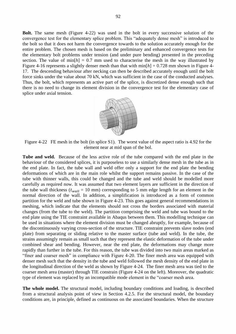
92

Bolt. The same mesh (Figure 4-22) was used in the bolt in every successive solution of the

convergence test for the elementary splice problem. This “adequately dense mesh” is introduced to

the bolt so that it does not harm the convergence towards to the solution accurately enough for the

entire problem. The chosen mesh is based on the preliminary and enhanced convergence tests for

the elementary bolt problems under tension (and under pure bending) presented in the preceding

section. The value of min[h] = 0.7 mm used to characterise the mesh in the way illustrated by

Figure 4-16 represents a slightly denser mesh than that with min[h] = 0.728 mm shown in Figure 4-

17. The descending behaviour after necking can then be described accurately enough until the bolt

force sinks under the value about 70 kN, which was sufficient in the case of the conducted analyses.

Thus, the bolt, which represents an active part of the splice, is discretized dense enough such that

there is no need to change its element division in the convergence test for the elementary case of

splice under axial tension.

Figure 4-22 FE mesh in the bolt (in splice S1). The worst value of the aspect ratio is 4.92 for the

element near at mid span of the bol.

Tube and weld. Because of the less active role of the tube compared with the end plate in the

behaviour of the considered splices, it is purposeless to use a similarly dense mesh in the tube as in

the end plate. In fact, the tube wall and weld offer only a support for the end plate the bending

deformations of which are in the main role whilst the support remains passive. In the case of the

tube with thinner walls, this could be changed and the tube and weld should be modelled more

carefully as required now. It was assumed that two element layers are sufficient in the direction of

the tube wall thickness ( = 10 mm) corresponding to 5 mm edge length for an element in the

normal direction of the wall. In addition, a simplification is introduced as a form of common

partition for the weld and tube shown in Figure 4-23. This goes against general recommendations in

meshing, which indicate that the elements should not cross the borders associated with material

changes (from the tube to the weld). The partition comprising the weld and tube was bound to the

end plate using the TIE constraint available in Abaqus between them. This modelling technique can

be used in situations where the element division must be changed abruptly, for example, because of

the discontinuously varying cross-section of the structure. TIE constraint prevents slave nodes (end

plate) from separating or sliding relative to the master surface (tube and weld). In the tube, the

strains assumingly remain as small such that they represent the elastic deformation of the tube under

combined shear and bending. However, near the end plate, the deformations may change more

rapidly than further in the tube. For this reason, the tube was divided into two main areas marked as

“finer and coarser mesh” in compliance with Figure 4-20. The finer mesh area was equipped with

denser mesh such that the density in the tube and weld followed the mesh density of the end plate in

the longitudinal direction of the weld as shown by Figure 4-24. The finer mesh area was tied to the

coarser mesh area (master) through TIE constrain (Figure 4-24 on the left). Moreover, the quadratic

type of element was replaced by an incompatible mode element in the “coarser mesh area.

The whole model. The structural model, including boundary conditions and loading, is described

from a structural analysis point of view in Section 4.2.5. For the structural model, the boundary

conditions are, in principle, defined as continuous on the associated boundaries. When the structure

93

is discretized by finite elements, the boundary conditions should be given at the nodes in a

consistent way. In the used element types, only the translational nodal degrees of freedom

representing three rectangular displacement components are used. Eqs. (4-1a) to (4-1c) are satisfied

on the internal boundaries cut through the symmetry planes, when the nodal displacements in the

direction of the normal vector of the associated plane are restrained in which case also the

associated rotations about the lines coinciding in the symmetry planes are prevented. The loading is

controlled through the prescribed axial displacement (Figure 4-5), which is increased step by

step in the computational procedure. This was done in Abaqus by enforcing the tip cross-section of

the tube to displace as a plane in the axial direction of the tube. The associated load can be

determined, for example, based on the requirement on axial equilibrium as explained in Section

4.2.4. Contacts between the end plate and the rigid surface at the transverse symmetry plane are

defined consistently with the frictionless normal contact discussed in Section 4.4. Then the

displacements, which coincide in the rigid plane and rotations are not constrained. The normal

(hard) contact itself is enforced in the procedure based on the surface-surface type of approach

available in Abaqus.

Figure 4-23. Parts and partitions near the weld on the left. Two element layers are used in the wall

of the tube independently of the mesh density in the end plate.

Figure 4-24. Medium meshes in the “active area” of the end plate and tube (on the left). The denser

and coarser meshes in the tube are connected with the TIE constraint available in ABAQUS.

94

Verification. The numbers of elements in the coarse, medium and fine meshes defined for the

convergence test for the elementary splice problem are given in Table 4-3. The medium mesh of the

end plate and the tube is shown in Figure 4-24. The refinements took place only in the end plate

representing the most active part in the response of the splice (S1), and in the “finer mesh area of

the tube” following the element division in the end plate as explained above. The FE mesh in the

bolt is sufficiently accurate such that it does not influence the results of the test. Moreover, the tube

in the “coarser mesh area” was assumed to play so passive a role in the splice response that its mesh

was kept as the same in all steps of the conducted convergence test.

Table 4-3 Number of elements in the 1/8-model of the tube splice in convergence test.

The results of the elementary convergence tests for the 1/8-model of the tube splice in tension are

illustrated in Figure 4-25, where the - , - and - curves are presented in the case of coarse,

medium and fine meshes. Thus, there are altogether nine curves in this figure: three curves for each

relation. In those curves, the axial load P, the bolt force B and the contact force C between the end

plate and rigid surface (see Figure 4-7) are all drawn as the functions of the tip displacement ,

which approximately equals according to Eq. (4-4) the generalised displacement defined by Eq.

(4-3). The curves obtained by the coarse mesh deviate somewhat from those achieved by the

medium and fine meshes, whereas the curves related medium and fine meshes follow almost the

same tracks apart from the large values of outside the area of main interest. For example, the

value of P obtained by the coarse mesh is about 7% larger than the one achieved by the medium

mesh when mm, whilst the latter one differs, in turn, less than 0.7% from that computed with

the fine mesh for the same . Moreover, the curve pairs (for - , - or - ) based on the medium

and fine meshes satisfy the condition expressed by Eq. (4-10a) and (4-10b) within a relatively small

tolerance value ( 1%) up to large values of ( 40 ... 50 mm). In the descending parts of the

curves in comparison, the difference between solutions by medium and fine mesh differs slightly. In

any case, the most interesting part of the response can be described almost similarly by the medium

and fine meshes based on the comparison of the associated curve pairs in Figure 4-25. Thus, the

solution obtained with the medium mesh can be judged to be converged, at least, in the interval of

the most interest. In other words, one can rely on the solution obtained with the medium mesh,

whereas the reliability of the solution with the coarse mesh is more questionable. In the other words,

the error caused by the discretization with the medium mesh can be seen as tolerable. It should be

noted that the ultimate (maximum) value of P of the axial force (limit point) could be equally

evaluated by the three meshes.

The contacts between the end plate and rigid plane the latter of which coincide in the transverse

symmetric plane at mid span are included in the elementary problem of the tube splice under axial

tension (type II). Every refinement of the convergence tests makes the description of contacts more

accurate, in addition to the description of the deformations (in the splice) through the denser mesh

of the finite elements. Thus, because the “converged mesh” as a result of the convergence tests was

found, it also involved acceptance of the discrete contact model used.

Mesh

Number of elements (N)

End plate

(Table 5-2)

Weld and active

area in tube

Bolt

Tube in the area of the

“coarser mesh”

(C3D20R or C3D8I)

Entire

model

Coarse 399 420 640 828 2287

Medium 2736 1680 640 828 5884

Fine 20928 6400 640 828 28796

95

Figure 4-25 Convergence test for the tube splice under axial tension (Abaqus).

4.3.5 Remarks

There are plenty of analysis examples in the program manual (Abaqus 2010), whose purpose is to

demonstrate to the analyst the capabilities of the program and, especially, the used elements.

However, the source code of the used Abaqus is not available to the public, which is common for

most commercial programs. Thus, code verification is not possible and, moreover, only

verifications through the benchmarks, or other numerical tests can be done. The models should be

built up in compliance with the recommendations given in the manual, which also concern the

regularity of the used finite element meshes. In this study, the used meshes fulfil the regularity

requirements quite nicely. The converged solutions found speak themselves for the acceptable

quality of the chosen meshes. All three elementary problems introduced above were modelled as

materially and geometrically nonlinear. The same elastic-plastic, strain hardening type of behaviour

(without plateau) was adopted in every analysis. Necking of the bolt, which was present in the

elementary problem of bolt in tension, is a strongly nonlinear phenomenon including high strain

values, which is definitely impossible to treat without geometrically nonlinear formulation. The

large rotations in the end plates required a nonlinear description of kinematics. Although it was not

possible to use exact solutions in the converged meshes were found in all cases. The FE models

used later in the analysis of splices problems are defined according to the convergence tests. Then

the medium meshes will be directly employed, although they are, very probably, not the most

efficient ones computationally. In any case, the assessed demands could be satisfied by them.

96

4.4 Validation and exploitation of the FE model

4.4.1 Introduction

The aim of the above verification procedure was to show that the solution of the splice

problem can be obtained by the discrete model in a reasonable way. How well the

mathematical model corresponds the actual physical event is another question, the answer of

which can only be obtained by comparing the computational results with the experimental

ones. In this study, the numerical models are employed in order to determine the bending

resistances of the tube splices. The principal aim was to enlarge the experimentally attained

(restricted) data computationally for splices under arbitrary biaxial bending. In order to create

a plausible model for this purpose, the validity of the used model must be proved first. The

validity of the model can be shown, in principle, through the sub-problems embedded in the

investigated problem correspondingly as it was done with the verification procedure in

Section 4.3. For example, the validation of the computational model could be based on the

same elementary problems used in the verification. However, we did not have the proper

experimental data on the elementary problems and, what is more important, the original idea

of this thesis was to study structural entities, which stand for a genuine 3D problem (not

reducible into 2D). These structural entities are the tube splices under biaxial bending, which

are the driving examples. Thus, the comparisons between the predicted bending responses of

these splices and the experimentally measured ones serve as the validation of the

computational model. In Section 4.5, the resistances based on the numerical analyses and

supported by the tests are furthermore derived for the splices under bending in the arbitrary

direction.

In the equilibrium path of a structure solved by the computational model, the equilibrium and

compatibility should prevail in every equilibrium configuration and the material behaviour

must obey the constitutive laws. In principle, the predicted response of the structure closely

imitates that of the related physical event when the computational model strictly corresponds

the actual structure. The differences between the model and actual structure may cause the

modelling errors, which can reside, for example, in the idealised boundary conditions and

geometry descriptions of the model, in the differences between the given and actual loading

or in the deficient ability of the constitutive laws to imitate the material response. The

influence of these factors may be difficult to study but the comparison between the different

models can help to understand some features of the obtained solution. Thus, although the used

computational model can finally be validated against the experimental data, the computational

comparisons can reveal the suitability of the used model to the intended purposes. In this

Section, the - curves and - curves are determined for the monotonically increased

vertical displacement. The - curves are defined using quantities, which were directly

measured in the tests, whilst - curves describe the flexural response of the splice between

the quantities, which were extracted from the tests by the described manipulation. It should be

noted that the loading scheme in the computation analysis was arranged under displacement

control instead of the load control. Thus the external load or forces like and has to be

determined by the post-processing of the FE analysis results. Although the main objective of

this thesis is to determine the resistances of the tube splices, the comparisons between

computed and measured quantities are made with the above mentioned full-range curves.

Then, in addition, the ability of the FE model to predict initial stiffness will be discussed.

Before the validity of the entire splice model is investigated by the comparison between the

97

computational and experimental - and - curves, the special features of the model

related to the simplified loading scheme, loading shelf (used in the biaxial bending tests) and

pretension of the bolts are discussed. Moreover, the response of the bolt in axial tension is

compared with the results of the separate bolt tests, which can be understood to represent a

complementary (or an elementary) case for the validation process of the splice model. The

simulations of the necking bolt can also be used to enlighten the role of the bolts in the splice

response. A simple definition through which the bolt failure caused by material fracture can

be predicted is discussed.

4.4.2 Simplifications and checks

After the verification of the model, the difference between the solutions of the mathematical

(continuous) problem and its numerical counterpart should be close to each other. Then an

essential error between the computational results and physical event may reside in the

erroneous modelling. In the pursuit of an “easily tractable model”, simplifications are usually

required. However, these simplifications may be also the sources of differences between the

physical event and the computational model. In an ideal case, an analyst can utilize the

simplified model such that the corresponding error is tolerable. If the simplifications are

overly rough, the model will lose its ability to describe the actual behaviour any more. Next,

the influence of the used simplifications on the predicted splice response is discussed.

The splice model is defined according to the idealised initial state the deviations from which

are not strictly known. The deviations from the actual initial state include the initial strains

and stresses, which mainly are a consequence from welding connecting the tube and end

plate. The gaps between the end plates of the splice related to contacts cannot be described

either in the initial state. However, the initial imperfections like these affect most on the

response of the splice at the beginning of the loading whilst the attained resistances are less

dependent on them. Particularly, this concerns the structural resistances, which are determined

by the plastic flow of the yielding mechanisms. According to the plasticity theory, for

example, the rigid-ideally plastic resistance is independent on the initial imperfections. In the

elastic-plastic models with large plastic deformations compared with the elastic ones, the

resistance of the structure can be approximated by the yield mechanism such that the role of

the initial imperfection remains as small.

The pretension forces of the bolts are approximated by the practical engineering formulas.

However, the influence of the possible erroneously evaluated pretension force on the splice

response, which also represents a deviation from the actual initial state, is very likely to be

restricted at the beginning of the loading. Moreover, the eccentrically placed bolts in the

model will probably cause only a small error. The possible contacts between the bolt and the

hole of the end plate are not decisive because the relatively short bolts are mainly in tension

and the role of the shear is negligible. Through the simplified bolt model (Section 4.2.2), the

necking of the bolts can be described as explained in Section 4.4.3, which is decisive when

the resistance of the splice under bending and in axial tension is predicted. The influence of

the bending moment on the maximum bolt force remains as small according to the FE

simulations presented in Appendices A5 and A6. It should be added that in the static analysis,

the cylindrical bolt model without threads can be seen reliable.

In addition, contacts between the end plates were modelled as classical contact model

including frictionless normal contact (Appendix A3), which probably deviates more or less

98

from the actual interaction. The contacts related directly the fasteners are also modelled in a

simplified way as explained in Section 4.2.2. It is probable that the deficiently defined

contacts in the initial state affect most the response of the splice at the beginning of the

loading. What is the influence of the used contact model on the resistance of the splice is not

studied in this thesis. However, the normal contacts can transfer the compressive forces over

the splice in the compression zone of the splice and, in addition, to describe the contact forces

related to the self-equilibrating prying action present in the tension zone. Thus, it is plausible

that the global response of the splice under bending and in axial tension can be predicted by

the employed contact model.

The material model, including strain hardening behaviour, was described according to the

approximate stress-strain curves based on the “discrete type of knowledge” of material

properties. Moreover, the assumed 3D elastic-plastic material model represents an idealisation

from the uniaxial model and, therefore, is a possible source for the modelling error between

the computed and physical behaviour. The essential structural phenomena are the strain

hardening response of the (strongly bent) end plate and necking of the bolts which cannot be

described by the stress-strain curves without the strain hardening behaviour for large (finite)

strain. The tensile tests arranged for the delivery lots by the manufacturer can be seen as

reliable such that the yield and ultimate strengths of the base material are known as discussed

before. This is the available material data in this research and it is used in compliance with

physical reasoning presented in Appendices A1 and A2. In any case, this data affect the

response of the splice when its stiffness is decreasing because of the gradually increasing

plastic deformation in the end plate and in the bolts. Thus, this data may possibly have a

decisive influence on the resistance value obtained by the numerical analysis by the 3D FE

method. The missing modelling of material fracture in the elastic-plastic analysis makes the

situation even more complicated to interpret.

Altogether, all the above mentioned deviations of the model from the actual splice constitute

the modelling error. To separately investigate their influence on the splice response would

require extra effort that was beyond the scope of this study. In this thesis, the success of the

model is investigated through the comparison between the predicted response and the

response measured by the tests on the considered tube splice. Finally, there is no other means

to judge the validity of the model than compare the computed values with the measured one.

In this study, the comparison is based fall up to the response of the structural entity

represented by the tube splice under biaxial and weak axis bending. The main objective is to

find out how the numerical model can be employed in order to extract the resistance values

for the splice under arbitrary biaxial bending. The associated failure curves for the moment-

moment interaction are determined at the end of Section 4. It is reminded that the principal

aim is to determine the resistances in the case of the arbitrary bending and other objectives are

only complementary although they can shed the light on some question related to the

responses of the end-plated splices.

Checks. Next, the rightness of some special features of the computational model or solution

procedure is studied by the checks related to the loading schema, loading shelf and pre-

tension forces. These checks are required to ensure that there is no discrepancy between the

splice models and the arranged tests.

The difference between the acting loads in the computational model and in the arranged test is

illustrated by Figure 4-8. In the model, the direction of the load remains constant, that it, the

99

load is strictly vertical, whilst the direction of the load deviates slightly from the vertical in

the test. The influence of this simplification on the resistance and stiffness of the splice was

discussed in Section 4.2.5. In order to avoid problems with the convergence in the iterations

of the solution algorithm, however, the analysis was arranged as displacement controlled. In

the related loading scheme, the vertical displacement of the splice is increased step by step

( . The corresponding vertical component can then be

determined in accordance with Eq. (4-8) based on the post-processing of the FE analysis

results. In addition, the horizontal component due to the enforced displacement can be

obtained as , which must remain as negligible in comparison with in order to

obtain acceptable results. In the simulation of biaxial bending test TE1 with the thinnest end

plate (splice S1 with the 10 mm end plate), the horizontal component increased with the

increasing such that the value was attained when the maximum vertical force

was reached ( ). Correspondingly, the value of was 0.54% of the

value of . In the case of tests TE3 with the thickest end plate (splice S3 with 20 mm end

plate), the value of the horizontal force was 0.25% of the value of the vertical force

. Thus, the horizontal force remained small in respect to vertical

force whether the end plate thickness of the splice was the thinnest or the thickest.

Obviously, the displacement controlled loading scheme was acceptable.

The intention is to analyse the considered tube splices under arbitrary biaxial bending through

the numerical model. The geometry of the employed splice model is shown in Figure 4-26 on

the left. In biaxial bending tests, however, the specimen has been modified by adding an extra

construction called a loading shelf, which is welded to the end plate as illustrated by Figure 4-

26 on the right. The shelf has been used in order to arrange stable loading as explained in

Section 3. In this case, the reasons for a possible difference between the model and the tests

originate already in the inconsistent testing arrangements made deliberately. In principle, the

comparisons between the tests that are otherwise similar but defined with and without the

loading shelf would reveal the possible differences caused by this “intentional modification”.

However, this was not done; whereas the influence of the loading shelf was evaluated purely

by the means of the numerical analysis. In Figure 4-27, the - curves of the accomplished

FE simulations for tests TE1 and TE3 (with shelf) and the - curves for splices S1 and S3

(without shelf) are shown in the same chart. There is no essential distinction between the

associated curves modelled with or without the loading shelf. Accordingly, the extra part

welded to the end plate in the compression zone has a negligible influence on the response of

the splice under bending.

Figure 4-26. Splice of interest (left) and as modified in the biaxial test (right).

100

Figure 4-27. Responses computed with and without the loading shelf.

The tightening moments of the bolts (torque) used in the arranged tests were given in Section

3. In the tests, the highest bolt(s) was (were) tightened with the tightening moment of

corresponding the pretension force of (Airila et al 2003). The bolts expected to be

tension bolts were pretensioned using the higher tightening moment of

corresponding bolt force . The exception was test TE1, in which all bolts had the

same tightening moment of . When the objective is to build an FE model for the

analysis of a tube splice under (biaxial) bending in an arbitrary direction, it would be practical

to define a computational model with the same pretension force in all bolts of the considered

splice. The splice can then be rotated about the longitudinal axis without any need to change

it. A numerical experiment was arranged in order to check if the splice can be analysed

without difference in the global response of the splice when the same pretension is used in all

bolts including the highest bolt(s) locating in the compressive zone of the splice. As a result

of this test, the analysis of splices with all bolts in the same pretension could be chosen as a

starting point when the splices under arbitrary biaxial bending were simulated.

4.4.3 Bolt model

Bolts with sizes and grades of M20-10.9 were used in the splice tests and were present in all

numerical analyses accomplished for the thesis. The ultimate load of kN was

determined as a mean value through three tensile tests. Unfortunately, no elongations were

measured during these tests conducted using entire M20 bolts. The broken bolts are shown in

Figure 4-28 below. The necking phenomenon precedes fracture in all cases. Anyway, the

limited ductility of the high strength bolts was seen by these tests. Next, the validation of the

bolt model is based simply on the value of the maximum bolt load obtained in the onset of

necking. A clue about the ultimate fracture of the bolt can be sought, in principle, by means of

101

the numerical simulations supported by the product information. A simple reasoning of this

kind helps to interpret the limitations of the elastic-plastic analyses.

Figure 4-28. Bolts M20-10.9 after tension tests, where only the ultimate load was measured

The geometry of the M20-10.9 bolts for the FE simulations is defined in compliance with

model B1 of Figure 4-2 using dimensions given in Figure 4-10 (according to splice S3). In the

employed model, the round cross-section with the tensile stress area As = 245 mm2 is related

to the diameter D = 2(As/π)0.5

= 17,662 mm. The stress-strain curve of the Ramberg-Osgood

type was built up for the bolts as explained in Appendix A2. In the discretised model, the

serendipity type of quadratic elements were employed according to the “enhanced mesh” with

min[h] = 0.7 mm illustrated by Figure 4-16.

Validity. Because of the restricted data about the bolt deformation, the validation of the FE

bolt model was based on the ultimate load value 278 kN as mentioned above. The

elastic-plastic simulation by the FE bolt model reproduced this value required for the onset of

necking quite accurately. The error was less than 0.1% when the computed value was

compared with the measured one. It should be emphasize that necking is partly a geometrical

phenomenon in its character (Roylance, 1996; Chakrabarty, 2006). Reversely, the material

response should be distinguished from the related kinematics when the (true) stress-strain

curve is determined. Thus, based on the nonlinear description of the kinematics introduced by

the FE model independently of the tests, the used model was able to predict the onset of

necking successfully. Although there were no data to validate the entire - curve, the

ultimate load value could be evaluated strictly by the FE simulation.

Discussion about fracture. According to the general deliverer’s information (Ferrometal

Inc.), the permanent extension in the case of the 10.9 bolt is about 9% in the tensile test in

compliance with the engineering interpretation. In the corresponding tensile test, the

associated initial gauge length is , where and are, respectively, the

diameter and cross-sectional area of the “round specimen” milled from the bolt. The

permanent elongation is measured when the broken parts of the bolt are fitted together.

Next, the bolt load causing the fracture is approximated coarsely based on this 9% limit such

that the force breaking the bolt is predicted from the results of the elastic-plastic analyses,

which do not include material fracture as an embedded feature. These simulations do no serve

directly as part of the validation process but shed light on the typical behaviour of the 10.9

bolts.

For the FE simulation, the free length of shank is defined first, such that

corresponding the initial gauge length of the related tensile test. Then, the bolt in tension

should “break” when the ratio reaches a value of 9%, understood as the permanent

elongation of the shank obtained by elastic-plastic FE analysis. The elastic part of the

elongation (elastic recovery according to the initial stiffness) must be taken off from the total

value reached in the - curve in order to obtain the correspondence with the 9%

elongation in the horizontal axis. In Figure 4-29 on the left, the breaking point is marked by

the circle in the simulated - curve, and, furthermore, the corresponding load (P = 233

102

kN) was determined from the vertical axis. Based on the localised nature of the necking

phenomenon, it is assumed that the fracture of the bolt is independent of the length of the

shank, which obviously holds unless the bolt is not too short. Then the second simulation of

the bolt model with the same cross-section of the shank ( ) but with a different length

( ) should produce the same load value P = 233 kN related to the “breaking

point” in the descending part of the - curve. As demonstrated on the right side of

Figure 4-29, the deduction in the opposite direction gives a permanent extension of 13.8%

when the length of the shank is L = 2.525D. The deformed shapes in the descending stages

produced by the FE simulations, when 233 kN, are shown in Figure 4-30, where the

contours of the maximum principal strains and the related values are also plotted. The largest

maximum principal strain in the bolt is approximately 49% in both cases. This implies the

local character of the necking in the bolts with different lengths. The largest principal strain is

obviously caused by the plastic deformations, such that its elastic part is then almost

negligible in respect to the plastic one. It should be noted that the computed maximum value

of von Mises stresses was approximately 1300 MN/m2 because of hardening of the steel

material at the “breaking point”.

The FE simulations of the bolts in tension were based on the stress-strain behaviour, which

should be distinguished from the geometrical phenomena as mentioned above. If the actual

stress and strain curve is not entirely known, the predicted dependence between the tensile

force and the elongation is more or less erroneous even if the kinematics have been described

correctly. The (pure) material response is not known after the onset of necking from the data

obtained by the tensile test. The related “post critical material behaviour” is usually described

through assumptions. The classical Ramberg-Osgood model includes the description of the

(endless) hardening behaviour (up to infinity). It should be noted that the stress-strain curve

including the “post-critical parts” of a tensile test can be determined (Ling, 1996) through the

method, which is too complicated for use in engineering practise if not properly automatised.

Figure 4-29. - curves for the bolts L= 5D and L= 2.525D = 44.6 mm.

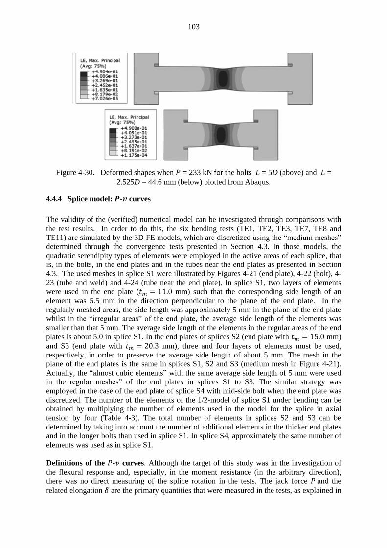
103

Figure 4-30. Deformed shapes when = 233 kN for the bolts L = 5D (above) and L =

2.525D = 44.6 mm (below) plotted from Abaqus.

4.4.4 Splice model: - curves

The validity of the (verified) numerical model can be investigated through comparisons with

the test results. In order to do this, the six bending tests (TE1, TE2, TE3, TE7, TE8 and

TE11) are simulated by the 3D FE models, which are discretized using the “medium meshes”

determined through the convergence tests presented in Section 4.3. In those models, the

quadratic serendipity types of elements were employed in the active areas of each splice, that

is, in the bolts, in the end plates and in the tubes near the end plates as presented in Section

4.3. The used meshes in splice S1 were illustrated by Figures 4-21 (end plate), 4-22 (bolt), 4-

23 (tube and weld) and 4-24 (tube near the end plate). In splice S1, two layers of elements

were used in the end plate ( mm) such that the corresponding side length of an

element was 5.5 mm in the direction perpendicular to the plane of the end plate. In the

regularly meshed areas, the side length was approximately 5 mm in the plane of the end plate

whilst in the “irregular areas” of the end plate, the average side length of the elements was

smaller than that 5 mm. The average side length of the elements in the regular areas of the end

plates is about 5.0 in splice S1. In the end plates of splices S2 (end plate with mm)

and S3 (end plate with mm), three and four layers of elements must be used,

respectively, in order to preserve the average side length of about 5 mm. The mesh in the

plane of the end plates is the same in splices S1, S2 and S3 (medium mesh in Figure 4-21).

Actually, the “almost cubic elements” with the same average side length of 5 mm were used

in the regular meshes” of the end plates in splices S1 to S3. The similar strategy was

employed in the case of the end plate of splice S4 with mid-side bolt when the end plate was

discretized. The number of the elements of the 1/2-model of splice S1 under bending can be

obtained by multiplying the number of elements used in the model for the splice in axial

tension by four (Table 4-3). The total number of elements in splices S2 and S3 can be

determined by taking into account the number of additional elements in the thicker end plates

and in the longer bolts than used in splice S1. In splice S4, approximately the same number of

elements was used as in splice S1.

Definitions of the - curves. Although the target of this study was in the investigation of

the flexural response and, especially, in the moment resistance (in the arbitrary direction),

there was no direct measuring of the splice rotation in the tests. The jack force and the

related elongation are the primary quantities that were measured in the tests, as explained in

104

Section 3. Due to the small inclination angle observed in all tests, and represents

approximately the vertical force and deflection (Section 3). On the other hand, the

computational curves are the - curves defined between the vertical force and the

deflection , which is the controlled quantity in the used computational loading scheme. Now,

- curves are simulated by the 3D FE model producing the - curves. For simplicity, both

the experimental and computational curves are called - curves here. Next, the experimental

and simulated - curves are compared with those obtained by tests TE1, TE7, TE11, TE2,

TE3, and TE8, which represent splices S1 to S4 according to Table 3-2. The slope of the -

curve at the beginning of the loading determines the initial stiffness whilst the maximum

value of the curve represents the resistance of the specimen. The latter one is either the load

value at the end of the test (when terminated) or the limit point given by the elastic-plastic

analysis. To interpret the differences between the test and computational results, it is useful

to remember that the roles of the tension bolt and end plate are decisive in the splice response.

The stiffer is the end plate, the larger role is left to the bolt and vice versa.

Test TE1/splice S1. The computed and experimental - curves of Figure 4-31 for biaxial

bending test TE1 corresponding to splice S1 ( 11.0 mm) are considered first. The

computed response was predicted quite well by the FE analysis up to the end of the test

although the model gave the somewhat stiffer response at the beginning of the loading. This

was possibly influenced by the negligence in the loading arrangements of test TE1 (see

Section 3). With the increasing load, the difference between the curves grows larger at first;

later, the computed and experimental curves meet each other and follow almost the same track

up to the point where the test was ended. Thus, the same slope in the strain hardening stage of

both curves was observed. The test curve ended because the load carrying capacity of the

specimen was reached and the test was terminated (Section 3). The computed curve continues

up to the limit point after significant deflection, which, finally, is followed by the descending

stage of the global response. This part of the computational curve is based mainly on the

“limitless hardening” of the elastic-plastic material response in the strongly bent end plate. In

the test TE1, the role of the bolts remains as secondary (no necking), which is confirmed by

the FE analysis (Section 4.4.5). In any case, the load obtained at the limit point was

clearly larger than the actual resistance observed in the tests (Table 3-8). Thus, the pure

elastic-plastic analysis cannot predict the resistance of splice S1 with 10 mm end plates in a

realistic way.

Test TE7/splice S1. The computed and experimental - curves of Figure 4-32 for weak axis

bending test TE7 (splice S1, with 11.0 mm) are in focus next. The computed response

predicts the initial stiffness well such that the analysis and test curve are closer to each other

at the beginning of the tests than in the case of test TE1. Altogerher, the initial stiffnesses of

the specimen with thin end plates can be predicted quite accurately by the FE model. With the

increasing load, the difference between the analysis and test curve becomes larger first, but

then they cross each other, and the test curve goes in the upper side up to the point at which

the test was ended. A deeper knee point starting the strain hardening stage was seen in the

computed than in the test curve (similarly as in the case of test TE1). The same slope in the

strain hardening stage of the computed and experimental curves can be seen in the figure. The

computed curve continues up to the limit point, after which the descending stage of the global

response follows. Again, the value of at the limit point was clearly larger than the actual

resistance observed in the test. The role of the strongly bent end plate was decisive in test TE7

whilst the bolts were in the secondary role as in test TE1. The significantly large deflection

was also predicted by the model as in the case of test TE1. It is noted that after termination of

105

the load controlled part of test TE7, it was continued as the displacement controlled one,

which revealed the outstanding ductility (deformation capacity) of the specimen at the

relatively high load level registered during the test up to its termination (Figure 3-12). From

this respect, the large deflection related to the limit point predicted by the elastic-plastic

analyses is not only theoretical speculation. However, the influence of the cracks in the end

plate observed at the end of the test TE7 (and in the displacement controlled part) is out of

reach of the elastic-plastic theory.


bending test TE11 (splice S4 with 11.0 mm) are considered. Splice S4 deviates from

splice S1 only because of the placing of the bolts, which are in the middle of the end plate

sides in splice S4 (not in the corners). The computed and experimental curves are quite close

to each other up to the end of the test although the model was slightly stiffer. The initial

stiffness of the specimen was predicted accurately by the FE model in the case of the flexible

end plate used also in splice S1. One can suggest that this accuracy is due to the relatively

small influence of the initial imperfections on the response of the thin end plate. With the

increasing load, the difference between the computed and test curve becomes somewhat larger

first, but then these curves meet each other and follow the same track briefly, after which the

test curve remains below the computed curve up to the point at which the test was ended. The

knee point of the computed curve is not so deep and the strain hardening stage is shorter than

in the case of splice S1. The maximum load value determined according to the limit point of

the computed curve is closer to the actual resistance obtained by the test than in the case of

splice S1. The mid-side bolts in splice S4 act more efficient than the corner bolts in splice S1

if judged according to the increased stiffness and resistances of the splice. Moreover, the

strain hardening stage seen very conspicuously in the “elastic-plastic - curves” for splice

S1 is no longer so obvious with splice S4; rather, the curve is more like an arch, which is,

probably, a result of the increased role of the bolts. Altogether, the computed and

experimental - curves in the splice S4 greatly resemble each other, and the difference

between them at the end of the tests obviously comes from the occurrence of the cracks in the

end plate not taken into account by the elastic-plastic model. The possibility of material

failure of the bolt (not seen in the test) also increases with the larger role of the bolts in the

splice response. This cannot be predicted by the elastic-plastic model although necking of the

bolt could be described in a plausible way (4.4.3). It must be noted that necking is likely to

happen before the material fracture of the bolt.


bending test TE2 corresponding to splice S2 ( 15.0 mm) are considered. The computed

curve implies a stiffer overall response, such that the curves do not cross each other. Again,

the slopes of the computed and experimental curves are equal in the strain hardening stage up

to the termination of the test. In any case, the computed initial stiffness (slope in origin) seems

to deviate from the observed one more than in the case of splices S1 and S4 with the thinner

(11.0 mm) end plates. An explanation for this can possibly be found in the increased influence

of the initial imperfections on the splice caused by the thicker end plate. The computed curve

continues further than the experimental one until it attains the limit point, after which the

descending stage of the global response follows. The value of at the limit point is

somewhat larger than the actual resistance observed in the tests but not so much as in the case

of splice S1 with the thinner end plate. The probable explanation is that with the thicker end

plate, the influence of the tension bolts on the splice resistance grows, such that the ultimate

106

0

50

100

150

200

250

0 50 100 150 200

P[k

N]

v [mm]

TE1, 10 mm plate

TE1, FEA

load can be predicted more closely, because necking can be simulated accurately by the FE

model (Section 4.4.3).

Tests T33 and TE8/splice S3. The experimental and computed - curves are shown for

splice S3 with a 20 mm end plate ( ) representing tests TE3 and TE8 in Figures

5-35 and 5-36, respectively. The end plates of splice S3 are the thickest ones amongst the

considered splices; therefore, the role of the bolts is expected to stand most out in the

response of splice S3, whereas the permanent deformations of the end plates remain smaller

than in the other tests. The computed response seems to be clearly stiffer than that observed in

the test. The initial imperfections, including residual stresses and deviation from the initial

geometry are not taken into account in the model, which probably explains the clearly smaller

initial stiffness of the actual splice at the beginning of the loading. Consistently, the influence

of the initial imperfections is more significant for splices with the thicker end plates than for

splices with the thinner end plates (in respect with bolts). With the increasing load, the

distance between the two curves grows first as larger but later, the computed and

experimental curves cross each other. The knee point preceding the strain hardening stage

almost disappears. The point at which the test was ended gives a slightly larger ultimate load

than the maximum load obtained in the elastic-plastic analysis. The reason for the larger

resistance in the test might reside in a longer plateau adopted to the stress-strain curve of the

end plate material in the model. However, the elastic-plastic 3D FE analysis of the splice can

predict the resistance of the splice satisfactorily because of the good predictability of necking,

which makes the response of the splice also as more predictable. The role of the bolts in

tension stands really out with the thicker end plates, such that the bolt behaviour decisively

affects the splice response. In tests, the failure of the specimen occurred with the somewhat

smaller value of deflection than according to the limit points of the computational curves.

However, the computed and experimental curves imply the less rotation capacity than in the

case of splices with the thinner end plates (A1 and S2). It is emphasized finally that both tests

TE3 and TE8 for splice S3 gave consistent results in the comparisons between the computed

and experimental curves.

Figure 4-31. Computational and experimental - curves of biaxial test TE1 (S1).

107

0

50

100

150

200

250

0 50 100 150 200

P[k

N]

v [mm]

TE7, 10 mm plate

TE7, FEA

0

50

100

150

200

250

300

350

400

0 50 100

P[k

N]

v [mm]

TE11, 10 mm plate

TE11, FEA

Figure 4-32. Computational and experimental - curves of weak axis test TE7 (S1)


108

0

50

100

150

200

250

300

350

400

0 50 100 150

P[k

N]

v [mm]

TE2, 15 mm plate

TE2, FEA

0

50

100

150

200

250

300

350

400

0 50 100

P[k

N]

v [mm]

TE3, 20 mm plate

TE3, FEA



109

0

50

100

150

200

250

300

350

400

0 50 100

P[k

N]

v [mm]

TE8, 20 mm plate

TE8, FEA

Figure 4-36. Computational and experimental - curves of weak axis test TE8 (S3).

Resistances. It is first reminded that the maximum load reached at the limit point by the

elastic-plastic FE analysis is defined as the computational resistance of the splice, whilst in

the conducted tests, the resistance was attained when the specimen fall down accidentally or

the test was terminated because of the almost horizontal response (Section 3).

The weakest estimates for the resistances were obtained in tests TE1 and TE7 for splice S1,

with the thinnest end plate and the corner bolts. Thus, this is obviously caused by the large

plastic deformations in the end plate, which make the specimen prone to fall down

accidentally, especially, when the related cracks appear. Then the computational model

cannot describe the behaviour, which may cause the actual specimen to lose its load carrying

capacity. In any case, the propagating permanent deformations in the largely bent end plates

are the main reason for the decreasing stiffness in splices like these. It should be noted that in

the Wheeler’s strong axis bending tests on tube splices under displacement control (Wheeler

et al. 1997a), a failure mode classified as “excessive deformations forcing the termination of

the tests” represented a failure typical for splices with flexible end plates. For those cases,

Wheeler suggested that the computational resistance could be defined according to the

constant deformation limit ( ) allowed to the splice. This nature of limit will be

discussed later and the suggestion for the resistance definition in the case of the considered

spices is given in Section 4.5 of this thesis.

It should be recalled first that the only difference between splices S1, S2 and S3 is in the

thickness of the end plate. The resistance could be predicted as a limit load by the FE

simulation best in the case of the thickest end plate; that is, in the case of tests TE3 and TE8

both representing splice S3. In test TE2 standing for splice S2 with the end plates of

intermediate thickness between splices S1 and S3, the resistance was obtained with the

110

0

10

20

30

40

50

0 0,5 1 1,5 2

P[k

N]

v [mm]

TE7, 10 mm plate

TE7, FEA

accuracy, which is somewhere between those obtained for splices S1 and S3. The role of the

bolts is increasing due to the increasing thickness of the end plate. Then the necking bolt must

be described accurately in order to obtain realistic FE simulation on the splice response

including the resistance prediction as a limit point. The resistance determined by test TE11 for

splice S4 was predicted much better than in the case of splice S1, which is otherwise similar

to splice S1 but assembled with mid-side bolts. The explanation for this can be found in the

greater stiffness and resistance of the bend end plate because of the more efficiently acting

mid-side bolts compared with the corner bolts.

Stiffnesses. The ability of 3D FE model to predict the initial stiffness can be investigated by

comparing the responses of splices S1 (TE7), S2 (TE2) and S3 (TE3) as a series with the

increasing end plane thickness through Figures 4-37 to 4-39, where the computational and

experimental - curves are drawn as focused on the beginning of the loading due to the

scaled axis. Clearly, the initial stiffness (i.e., the slope of the - curve) can be estimated best

with the thinnest end plate (S1), worst with the thickest (S3) and between those in the case of

splice S2 with the intermediate thickness of the end plate. Thus, the thicker the end plate is,

the less accurately the FE model predicts the initial stiffness. This can be interpreted such that

the influence of the deficiently described initial by the FE model has larger influence on the

splice stiffness when the end plate is thicker. To remove the possible modelling error through

the better description of the initial state, a proper investigation of the imperfections would be

required, which is not included in this thesis. It should be noted that also Wheeler et al (1998)

reported poor ability of the idealised splice model to predict the initial stiffness in the case of

stiff end plates.

Figure 4-37. Computational and experimental - curves as scaled at the beginning of the

loading for test TE7 ( . The stiffness of the splice can be predicted nicely. The

preliminary loading cycle is shown in the figure.

111

0

10

20

30

40

50

0 0,5 1 1,5 2

P[k

N]

v [mm]

TE3, 20 mm plate

TE3, FEA

Figure 4-38. Computational and experimental - curves at the beginning of the loading in

for test TE2 ( .

Figure 4-39. Computational and experimental - curves at the beginning of the loading can

for test TE3 ( . The stiffness of the splice can be predicted poorly.

Ductility. From the plasticity theory point of view, ductility of a structure can be defined as

its ability to deform without collapsing in the required load level. A definition of this kind is

112

usable in structural steel design. The deflection of the specimen attained with the

maximum load can be used as an approximate measure for ductility, which can be

determined whether the - curve is attained by the test or by the elastic-plastic 3D FE

analysis. In the tests, however, the loss of ductility may happen as prematurely in respect with

that predicted by the FE analysis. In the case of splice S1 with the flexible end plates, the

reached deflection was clearly smaller than that predicted numerically. In the related

tests TE1 and TE7, cracking was observed at the end of the tests after large plastic

deformations of the end plate. However, the specimens showed large ductility such that the

deformation capacity of splice S1 would be sufficient for structural purposes, in compliance

with EC3 (Section 6.4.2 of EN1993-1-8). Thus, the observed cracking would not restrict the

usability of the splice S1 in the plastic design (in global plastic analysis). It should be noted

that in Appendix A6, the large deformations causing finally cracking were demonstrated in

the case of splice S1. Splices S2 and S3 with the thicker end plates were less ductile according

to the reached value of although no cracks were observed in the related tests. The FE

model was able to predict of splice S3 quite accurately because of the ability of the

model to describe necking of the bolts in a satisfactory way. Moreover, of splice S4 with

the same end plate thickness as used with splice S1 was predicted coarsely, but more

accurately than in the case of splice S1 because of the larger stiffness of the tension flange

with mid-side bolts despite severe cracking of the end plates in related test TE11. It is denoted

that all the tested splices showed significant rotation capacity, which was larger than 50

in the arranged tests (Section 3).

Validity of the model. Based on the comparisons between the test and computed curves

presented above, a simple answer to the validity of the elastic-plastic 3D FE model cannot be

obtained. The ultimate resistance of the splice was predicted in a satisfactory way in the case

of the thick end plates when necking bolt had a determinate role in the gradual decreasing of

the stiffness. Reversely, the elastic-plastic model fails to predict the resistance of the splice as

a limit load in the case of thick end plates. On the other hand, the initial stiffness of the splice

can be predicted well in the case of flexible end plates whilst the increasing stiffness of the

end plates in respect to the used bolts seems to results in the poorer prediction of the initial

stiffness. In any case, this physical reasoning presented above helps when the numerical

results are interpreted.

4.4.5 Splice model: - curves

The performance of the numerical, elastic-plastic 3D FE model was considered through -

curves although the main interest is in the flexural response of the splices. Next, both the

computational and experimental moment-rotation curves ( - curves) of the considered

splices are compared with each other. This discussion about the flexural response completes

the primary validation presented above.

Definitions of the - curves. Test curves were determined as explained in Section 3. The

value of the bending moment at mid span was calculated through Eq. (3-3). The rotation of

the splice was evaluated, in turn, in accordance with Eq. (3-5) such that the deformations

caused by bending and shear in the beam were excluded. It should be noted that possible

shear force in the splice was taken by friction between the end plates. The computed curves

were determines as described in Section 4.2.5. The resultant moment was calculated by Eq.

(4-9) provided that the reaction force was determined first through the post-

processing of the FE results because of the displacement controlled loading. The splice

113

rotation was determined analogically with the generalised beam theory according to Eqs. (4-

6) and (4-7). Then, the value of the rotation is integrated over the (welded) beam cross-section

between the tube and the end plate without the need to acquire information about the tube

deformations outside the splice. It is emphasized that the used splice rotation represents an

orthogonal mode which is independent on the other generalized deformations defined for the

tube. When the analysis of joints is embedded in the analysis of frames with thin walled (open

or closed) beams, this definition would be the desired one. It must be noted yet that the -

curves represent directly the scaled - curves determined through Eq. (3-3) and Eq. (3-4)

the latter of which defines the connection between and the gross rotation . As a

consequence, the experimental - curves would behave in relation with the computed -

curves similarly as in the above presented comparison of the - curves. The difference

between the gross rotation and the splice rotation is relatively small (Tables 3-10 and 3-

11) such that the - curves coarsely represent the - curves.

The experimental and computational - curves are presented for all splices in Figures 4-40

to 4-45. In these figures, the “reference limit” of is marked by the vertical dotted

line. The value of for the splice rotation represents a large rotation, which is reached

in the practical joints only exceptionally. Wheeler has exploited the rotation limit of

as a value with which the resistance of the joint is obtained in the case of the excessive

deformations (Wheeler et al, 1997b, Wheeler 1998). In order to keep track of the bolt

behaviour in the splice during loading, those points of the computed - curves, where the

most strained tension bolt(s) obtain their maximum bolt force are marked by triangles and

those points related to possible bolt break ( 233 kN, Section 4.4.3) are marked, in turn, by

circles. The development of the bolt forces is discussed also in Appendices A5 and A6, where

the complementary results of the numerical simulations on the splice responses are presented.

In addition, the resistance determined by the 3D component method (Section 5) is marked by

the horizontal dashed line in each figure.

Tests TE1/S1. The experimental and computational - curves for splice S1 based on

biaxial bending test TE1 ( ) and its FE simulation, respectively, are shown in Figure

4-40. The considered splice belongs to the series S1, S2 and S3 with similar layout and the 10,

15 and 20 mm end plates, respectively. Splice S1 has the thinnest ( ) end plate

in this series. The computed - curve has the linear portion, knee area and strain hardening

portion the latter one of which is almost straight. Finally, a limit point with is

attained, followed by the descending response called the post-ultimate portion of the -

curve. These stages cannot be distinguished in the experimental - curve of test TE1 as

clearly as in the computational - curve, or they are totally missing. Firstly, the more

gradual decrease of the stiffness can be seen in the experimental - curve between linear

and strain hardening portions. This is related to the earlier onset of the plastic deformation in

the specimen not taken in the account by the idealised model. Secondly, the premature failure

has been ended the experimental - curve much before the limit point is attained in the

computational curve. In any case, the experimental curve meets the computational one, after

which it turns almost horizontal just before the termination of the test. The largest rotation

(117 mrad) attained in the tests implies the remarkable deformation capacity being much

larger than the reference limit value of used by Wheeler et al (1998). The FE

solution shows an extremely long strain hardening portion with the rotation of 246 mrad

reached at the limit point. In addition, the bending resistance predicted by the elastic-plastic

model is much larger than the experimental value due to this long strain hardening portion.

114

The onset of necking in the most strained tension bolt (marked by the black triangle in Figure

(4-40) appears in the computational curve at the load level not even reached in the test. Thus,

the tension bolts must have a passive role in test TE1 and, on the other hand, failure must be

related to the strongly bent end plates with large plastic deformations. It should be recalled

here that, in a load-controlled test, failure is usually a violent occurrence, which is typical for

overloaded structures in the real world.

Test TE7/S1. Another pair of the experimental and computational - curves for splice S1

is presented in Figure 4-41 in the case of weak axis bending test TE7 ( ). The strain

hardening portion now can be identified more clearly from the test curve than in the case of

test TE1. During this stage, the test curve is somewhat higher but approximately has the same

slope as the computed curve until the premature failure occurs in the test. The maximum

rotation reached in the test was large ( ), which still is much smaller than that the

rotation related to the limit point of the computed curve ( ). The bending resistance

predicted by the elastic-plastic model is significantly larger than the experimentally

determined one due to the long strain hardening portion. It should be noted that the large

gross rotation of about was obtained for the splice under displacement controlled

load arranged after test TE7. During this extra part of the test, however, an almost constant

load level prevailed (Figure 3-12), which implies the remarkable ductility of the specimen. It

should be noted that the onset of necking of the most strained tension bolt (marked by the

black triangle in Figure 4-41) occurs at quite a late stage in the hardening portion of the

computational curve at a higher load level than reached in the test. Obviously, the response of

the end plates as the “excessively deforming” part of the splice has the main role in test TE7.

Test TE2/S2. The experimental and computed - curves for splice S2 based on biaxial

bending test TE2 ( ) and its FE simulation are shown in Figure 4-42. Splice S2 has

been equipped with 15 mm end plates representing the intermediate thickness in the series of

three splices S1 to S3 with corner bolts. The strain hardening portion in the computed -

curve is shorter than the corresponding one in the simulation on splice S1 with the more

flexible end plate. The computed curve goes somewhat above the experimental one in the

strain hardening portion. The onset of necking in the two most strained tension bolts (marked

by triangles in Figure 4-42) happens already at the beginning of the strain hardening portion

of the computational curve, which implies the larger role of the bolts in the splice response

than in the case of splice S1. Following the onset of necking, the bolt behaves in an unstable

way, such that the bolt load is decreasing. In spite of the two necking bolts, splice S2 can still

carry the increasing bending moment probably because of deceasing prying (analogy with

splice in axial tension, see Appendix A4). Finally, with the decreasing ability of the bolts to

carry load turns also the global response to the descending stage through the limit point.

Necking of the lowest tension bolt is predicted to start approximately at the load level, which

was obtained also in the test. This is in compliance with the observation of necking of the

lowest bolt in the inspection of the specimen after the test.

Tests TE3 and TE8/S3. The experimental and computed - curves are shown for splice S3

based on tests TE3 ( ) and TE8 ( ) in Figures 4-43 and 4-44, respectively. Splice

S3 has been equipped with 20 mm end plates, representing the thickest ones used in the series

of three splices S1 to S3 with corner bolts. In both computational curves for splice S3, the

response after the knee area is present without an essential increase in the value of the

bending moment . The relatively stiff end plate, in respect to the stiffnesses of the (tension)

bolts, causes the increased role of the bolts compared with splice S2 and, especially, with

115

0

10

20

30

40

50

60

0 50 100 150 200 250 300 350 400

M[k

Nm

]

θ [mrad]

TE1, 10 mm plate TE1, FEA

B1 (max) B1 (ultimate)

B2 (max) 35 mrad

M 55 ,COM = 33.5 kNm

splice S1. This is in compliance with the observation that the advanced necking in the lowest

bolts could be seen in the visual inspection after tests TE3 and TE8 (Section 3). In the

simulations, the onset of necking in the most strained bolt (B1 and B2, see Appendix A6)

marked by triangles in the curves was predicted to occur at the load level, where the

experimental curves are still increasing. As a result of the significant role of the bolts, necking

of which could be predicted accurately, the maximum moment values obtained by the

computational model were close those reached in the tests.

Test TE11/Splice S4. The experimental and computational - curves for splice S4 based on

biaxial bending test TE11 ( ) and its FE simulation are shown in Figure 4-45. Splice

S4 ( 11.0 mm) is otherwise similar to splice S1, but the bolts are placed on the mid-sides

of the end plates in it. The knee area between the elastic and strain hardening portion, which

can be clearly identified in the computed curve, is deeper in the computational than in the test

curve. The computed and experimental curves are quite near to each other such the difference

between them is largest in the knee area. In the strain hardening stage, the test curve is

slightly below the computed one almost touching it until the experimental curve turns

horizontal before the termination of the test. The maximum point of the computed - curve

was obtained at a load level somewhat higher than that reached in the test. Necking of the

most strained bolt, which is marked by the triangle in the computed curve, was predicted to

occur roughly at the same load level, where the ultimate resistance was attained in the tests. In

addition, the onset of necking in the second most strained bolt followed quite rapidly after the

maximum bolt force has been reached in the most strained bolt in the computational model.

Nevertheless, the responses of both the bolts and the end plate were obviously utilised more

evenly in splice S4 with mid-side bolt than is splice S1 with corner bolts. The numerical

simulation of splice S4 is discussed more in Appendix A6.

Figure 4-40. Computational and experimental - curve for test TE1 (S1).

116

0

10

20

30

40

50

60

0 50 100 150 200 250 300 350 400

M[k

Nm

]

θ [mrad]


B1, B2(max) B1, B2 (ultimate)

35 mrad

M 90 ,COM = 28.8 kNm

0

10

20

30

40

50

60

70

80

90

100

0 50 100 150 200 250 300 350 400

M[k

Nm

]

θ [mrad]


35 mrad B1 (max)

B1 (ulimate) B2 (max)

B2 (ultimate)

M 55 ,COM = 47.0 kNm



117

0

10

20

30

40

50

60

70

80

90

100

0 20 40 60 80 100 120

M[k

Nm

]

θ [mrad]


35 mrad B1 (max)

B1 (ultimate) B2 (max)

B3 (max)

M 55 ,COM = 77.4 kNm

0

10

20

30

40

50

60

70

80

90

100

0 20 40 60 80 100 120

M[k

Nm

]

θ [mrad]


35 mrad B1,B2 (max)

B1, B2 (ultimate)

M 90 ,COM = 66.3 kNm



118

0

10

20

30

40

50

60

70

80

90

100

0 20 40 60 80 100 120

M[k

Nm

]

θ [mrad]


35 mrad B2 (max)

B1 (max) B1 (ultimate)

M 55 ,COM = 50.5 kN

Figure 4-45. Computational and experimental - curve for test TE11 (S4)

Resistances and initial stiffnesses. To complete the previously presented observations on the

- curves, the values of the computed and experimentally determined resistances (moments)

and initial stiffnesses are gathered in Tables 4-4 and 4-5. The computational bending

resistance is defined according to the limit point of the - curve, whilst the

resistance is defined as the maximum moment reached in the (load controlled)

test (Tables 3-10 and 3-11). The predicted resistances are closest to the experimental

ones ) in the case of tests TE3 and TE8, representing splice S3 with the thickest end

plate ( ) in the series of splices S1 to S3 with corner bolts. The absolute value of

relative error is less than 5% in both cases, which is quite a satisfactory result. The resistances

obtained in tests TE3 and TE8 are higher than those predicted by the FE analysis, which is

possibly caused by the missing plateau of the actual stress-strain behaviour in the end plate

near the weld. The 3D FE model fails most when predicting the resistances of tests TE1 and

TE7, representing splice S1 with the thinnest end plate ( ). The increasing

response during the long strain hardening portion in the elastic-plastic model results in

moment resistances that are 23% and 15.5% larger than those observed in tests TE2 and TE7,

implying the premature failure of the specimen before the computational plastic limit points

was reached. In test TE2 representing splice S2 with the intermediate thickness of the end

plate ( ), the relative error of the predicted resistance was 12.5 %, which is

between those attained for splices S1 and S3. In the case test TE11, representing splice S4

with 10 mm end plate but the efficiently located bolts in its flanges, the relative error is ,

which also is between those attained for splices S1 and S3. The suggestion is:

The resistance predicted by the elastic-plastic model as the plastic limit point is most

accurate when necking of the bolts appears in the splice response. With an increasing

role of the deforming end plate in the splice response, the ability of the elastic-plastic

model to predict the resistance seems to weaken.

119

Additionally, it is discussed about the (initial) stiffnesses. The predicted stiffnesses ( )

are determined in compliance with Eq. (3-8) based on the - curves of Figures 4-40 to 4-45

such that kNm and kNm. The experimental values ( ) can be found in

Tables 3-12 and 3-13 based on intervals given in those tables. If the difference

would be shortened, then somewhat but not essentially larger values for the stiffnesses would

have been obtained. Finally, all stiffnesses are shown in Table 4-5. The computational model

of the splice is stiffer than the actual splice in every considered case. The values of the ratio

range from 1.2 to 5.1. Because the elastic modulus is approximately the same

for all steel grades used in the splices, the difference in the stiffness values must result mainly

from the other differences from the computational model and test. The FE model was based

on the idealised boundary conditions and geometry and no other initial imperfection (initial

strains and stresses) are described either. Obviously, these imperfections of the actual splice

made it more flexible than the idealised one. In the series of tests S1 to S3 with the corner

bolts, the best prediction for the initial stiffness was obtained for the splices with the thinnest

end plates (S1). The largest values 5.1 and 3.0 of the ratio were obtained,

respectively, in the case of the thickest end plate (S3). The stiffness of splice S2 with the

intermediate end plate thickness was predicted somewhat less accurately than the stiffness of

splice S1 against biaxial bending moment. Altogether, the thicker the end plate of the splice

is, the less accurately the initial stiffness can be predicted. In addition, the FE model gives a

satisfactory estimate to the initial stiffness of the biaxial bending test TE11 with 10 mm end

plate and without the corner bolts. The “additional suggestion” is:

The description of the imperfections is more significant for the splice with thicker end

plates than for the splice with thin end plates when the initial stiffness is evaluated.

Table 4-4. Comparison between the computed and experimental resistances.

Splices with four-bolt layouts Tests

[kNm]

[kNm] [%]

S1, Corner bolts, 11.0mm TE1, 55.6 45.8 23

TE7, 50.0 43.3 15.5

S2, Corner bolts, 15.0mm TE2, 70.3 62.5 12.5

S3, Corner bolts, 20.3mm TE3, 96.9 99.0 -2.1

TE8, 85.9 90.3 -4.9

S4,Mid.-side bolts, 11.0mm TE11, 80.6 75.5 6.7

Table 4-5. Comparison between the computed and experimental initial stiffnesses.

Splices with four-bolt layouts Tests

[kNm/nrad]

[kNm/nrad]

S1: Corner bolts, 11.0 mm TE1, 4.8 2.2 2.2

TE7, 3.6 3.0 1.2

S2: Corner bolts, 15.0 mm TE2, 11,0 4.7 2.3

S3: Corner bolts, 20.3 mm TE3, 21,3 4.2 5.1

TE8, 13,9 4.7 3.0

S4: Mid.-side bolts, 11.0 mm TE11, 15,4 12.0 1.3

NOTE = Angle as measured ftom the weak axis is .

120

0

20

40

60

80

100

0 50 100 150 200 250 300

M[k

Nm

]

θ [mrad]

TE1 (10mm plate)

TE2 (15mm plate)

TE3 (20mm plate)

TE11 (10mm plate, mid-side bolts)

4.4.6 Remark on the computed - curves

The computed - curves of four biaxial bending tests (TE1, TE2, TE3, TE11) on tube

splices are gathered in Figure 5-47. In Figure 5-48, these curves are scaled to show the

beginning of the loading, such that the initial stiffnesses can be easily seen. The resistance of

the splice is natural to define according to the limit point (corresponding the maximum

bending moment) obtained in the analysis. The initial stiffness is defined as slope of the curve

in the origin.

The comparisons of the curves reveal in one glance the efficiency of the four-bolt layout in

respect to the mid-side bolts in comparison with those assembled with the corner bolts. This

efficiency concerns both the resistances and stiffnesses of the splices. In both cases, splice S4

with 10 mm end plate behaves as “the second strongest and stiffest” splice, falling between

splices S2 and S3 provided with the 15 and 20 mm end plates, respectively. The group of the

computational curves of Figure 5-46 is analogous with the group of the experimental curves

drawn for the biaxial bending tests in Figure 3-13.

The simulations on the splices S1, S3 and S4 under biaxial bending are presented and

discussed with more detail in Appendix A6. In Appendix A5, all splices (S1 to S4) under

axial tension are considered based on FE analysis results. It should also be noted that contacts

between the end plates are discussed in Appendix A4 related to the analysis results of splice

S1 in axial tension.

Figure 4-46. Computed - curves for the tests with biaxial bending only. The limit points

are marked by circles.

121

Figure 4-47. Computed - curves scaled for comparison of the initial stiffnesses.

4.5 Failure curves for arbitrary biaxial bending

The accomplished computational analyses of the considered tube splices are based on the

elastic-plastic behaviour of its steel parts, which represents the traditional and prevailing

approach through the FE analyses of structural steel joints in the literature. For example, the

FE analyses in all referred articles in this study are based on the elastic-plastic material

response. In this context, the decreasing of the splice is seen as a result from the gradually

increasing plastic deformation in the splice is the primary reason for the failure. Then, for

example, the accidentally opened cracks may be the secondary reason for the failure of the

specimen. The weakness of the elastic-plastic solution is related to its missing ability to take

into account the material fracture or other possible reasons causing the premature failure of

the specimen with the low stiffness in the simulated tests. If the resistance is determined

according to plastic collapse load by the elastic-plastic analysis, there might be a discrepancy

between the predicted and measured resistances. However, the elastic-plastic response

predicted by the FE analysis can describe the strain hardening stage in the splice response in a

plausible way after the knee point up to the failure occurred in the test as shown by the

comparison between the computed and experimental curves in Section 4.3. In principle, this

property can be utilised when the resistance values are predicted based on the results of the

elastic-plastic FE analyses.

The tests on tube splices under strong axis bending (Wheeler et al 1997a) and the associate

elastic-plastic FE simulations (Wheeler 1998, Wheeler et al 2000) represent close forerunners

to this study. The procedures suggested in ”Wheeler’s researches” for the determination of

122

failure of the tube splices based on the FE analysis results can be used as reference for the

corresponding procedures presented now. The Wheeler’s suggestion on the constant limit of

for the maximum allowed rotation for the excessively flexible splices is abandoned

hare and the resistances determined through the load controlled tests are preferred (the limit of

is drawn in Figures 4-40 to 4-45 for comparison). In addition, the definition of the

failure mode, which is based on the same constant value (limit rotation) independently of the

splice itself, do not represent a solid engineering reasoning. The use of a constant limit

rotation does not take into account, for example, that the resistance of the splice is decisively

dependent on the end plate thickness in respect to the used bolts. Wheeler also suggested a

threshold condition according to which ”the bolts are deemed to have failed when the average

strain in the threaded region on the bolts exceeds 3%”. A condition like this comes into use

when the end plate is thick (stiff) enough in respect to bolts. However, a definition of this

kind is quite problematic because of the local nature of the necking phenomenon illustrated by

Figure 4-30. According to simple reasoning based on the associated FE analyses, the varying

length of the threaded region does not change the tension resistance in the case of the used

full threaded bolts. It should be noted that the speculation about bolt fracture presented in

Section 4.4.3 might offer another simplified approach to the bolt failure. However, a

speculation of this kind can be seen only as secondary when the experimental data on the

resistance of the whole splice is available. The advanced definition of the threshold condition

for the bolt deformation would require the modelling based on the fracture mechanics, which

are outside the scope of this thesis.

In this study, the aim is to investigate the suitability of the component method of EC3 for the

three-dimensional analysis method of the tube splice under arbitrary biaxial bending. The

associated task is to show that the reserve against failure over the bending resistance

in the arbitrary direction predicted by the component method is sufficient. In the subscript of

, the angle refers to the direction of the resultant bending moment in compliance

with Figure 4-3. The empirical resistance was obtained directly in the six tests

arranged on tube splices under biaxial ( and weak axis ( bending. These

tests belonged to the same group of tests, which was arranged in order to determine the

resistances of four different splices S1 to S4 representing the driving examples of this study.

A special criterion for failure of each considered splice is derived in Section 4.5. These

criteria are intended for the purposes of this study only such that the resistances of these

splices in the arbitrary direction can be extracted through the post-processing of the results of

the elastic-plastic FE analyses. In the required analyses, the tube and its splice have to been

rotated around the tube axis. Then the direction of the resulting biaxial bending moment is

correspondingly changed whilst the other features of the model are kept constant. Finally, the

failure curves representing the numerically expanded validation data were fitted to the test

points according to the suggested criteria.

4.5.1 Definitions and procedure

Next, the intention is to formulate the bending resistances in arbitrary directions as a moment-

moment interaction curve - between the rectangular components and of

the resultant bending resistance . The resistance and its components in the weak and

strong axis directions are marked, respectively, as , and for simplicity. The

rectangular components and are related to the resistance through

123

. (4-11)

and to the angle , which gives the direction of , as

, (4-12

where is defined in compliance with Figure 4-3 (far right), such that its values and

correspond with strong and weak axis bending, respectively. It is noted that the angle

, which defines the rotated position of the test specimen (Figure 3-7), is complementary to

. The resistance must be known in sufficiently many directions in order to draw the

interaction curve of biaxial bending going through the failure points in the moment-moment

plane. It is emphasised that the resistance represents the distance from the origin to the

failure point in the moment-moment plane.

The computational - curves shown in Figures 4-40 to 4-45 were obtained as a result of the

FE analysis, and they describe the rotational response of the tube splice based on the elastic-

plastic material behaviour. The maximum moment written as a function of

the angle defines an interaction curve called here elastic-plastic failure curve, or

, (4-13)

which can be written also in parametric form

and , (4-14)

which is suitable for being used in the moment-moment plane. The comparisons between the

computed resistances and those obtained by the testing (Table 4-4) indicate that the elastic-

plastic failure curve might be realistic only for splices S3 with the stiffest end plate, whereas

it fails in the case of other splices with thinner end plates as discussed above. Thus, a failure

curve of this kind is expected to be located too far from the origin when determined for splice

S1, S2 and S4. Then, Eq. (4-14) must be rejected and replaced with the one based on better

criteria for the failure of the splice, which will be judged through the post-processing of the

elastic-plastic analysis results, according to a simple fitting procedure suggested next.

By assuming that the considered splice loses its load carrying capacity at the constant value of

the rotation , independently of the direction of the bending moment, the associated

moment in each computational - curve defines failure of the splice.

The fitted elastic-plastic failure curve can then be presented in the - plane as

and . (4-15a)

By introducing a coefficient , which takes into account the correction in the

resistance value due to the dependence of the rotation on the changing direction

of the bending resultant, Eq. (4-14a) gets an improved form

and , (4-15b)

124

where the dependences of and on angle and is not shown particularly. Of course,

Eq. (4-15b) would be unnecessary if the dependence were embedded through

directly in (4-15a). Unfortunately, the “correction coefficient” is

not known in which case Eq. (4-15a) replaces Eq. (4-15b) consistent with the simplification

that value of is constant.

In the used procedure, the failure curve represented by Eq. (4-15a) is fitted to a test point such

that

and , (4-16)

where and define a test point with the smallest distance from origin.

Consequently, the corresponding value of in the computed - curve is used in all

directions . The associated failure curve is entirely “on the safe side” only if the test that

gives the absolute minimum value for is included, which cannot be guaranteed in general.

However, a reasonable approximation on the resistance is obtained through (4-16), because

the resistance grows slowly with the increasing deformations in the large values of the

rotation angle. It should be noted that all equations from (4-12) to (4-16) can be expressed as

a function of the complementary angle instead of . For example, Eq. (4-12)

then has the form ). In the - plane angles and β are defined as

shown in Figure 4-48.

4.5.2 Failure curves for splices S1 to S4

Next, the failure curves will determined for all splices S1 to S4 in order to describe the

bending resistance for arbitrary . These failure curves are drawn by connecting

the computed points ( , ) with straight lines. They are based on solutions obtained in

the directions and such that and

correspond, respectively, with weak and strong axis bending in the first quarter of the

coordinate plane. Because of the symmetry, the failure curves can be expanded to three other

quarters of the associated coordinate plane. Although the used division of the failure points is

sparse, denser segmentation would not provide essentially more information.

Splice S1. The “large yielding of the end plate” was observed in biaxial and weak axis

bending tests TE1 and TE7 (with 11.0 mm), representing the same splice S1 but with

different inclinations from vertical. The clearly larger deformation of the end

plates was obtained at the limit point of the elastic-plastic simulation than in the test. The

rotation reached was 117 mrad in test TE1 (Table 3-10), whereas the computed rotation at the

limit point was about 250 mrad. The dashed line in the - plane in Figure 4-48 stands for

the (pure) elastic-plastic failure curve of the splice under arbitrary biaxial bending in

compliance with Eq. (4-14). Both failure points related to tests TE1 and TE7 are clearly inside

this theoretical curve. The premature failure of splice S1 can be predicted more reliably by the

curve, which is determined through the procedure based on Eq. (4-16), such that it is fitted to

the test point with the smaller distance from origin obtained by the two tests. As seen from the

figure, the failure point related to test TE1 gives the “inner curve”, which is closer to the

origin in the - plane than that fitted to test TE7. Only the former is shown in the figure.

The associated value of the rotation is about 100 mrad, which is employed when the

125

resistance value in each direction is determined according to the related - curve

determined by the elastic-plastic analysis. For comparison, the failure curve with the rotation

limit is also drawn in Figure 4-48 as a dotted line. This limit of ,

which has been suggested in the literature (Wheeler 1998) as a criterion to be used when the

“numerical ultimate moment” is defined in the case of the failure mode associated with the

deformation failure (Section 3.4.1). The resistances based on Eq. (4-15a) with

is about 80% to 90% of those predicted with .

Splice S2. The thickness of the end plates of splice S2 ( 15.0 mm) represented the

“intermediate thickness” between those used in splices S1 and S3. As observed in the series

TE1, TE2 and TE3, the end plate deformed less than in test TE1 and more than in test TE3.

For splice S2, the failure curve Eq. (4-14) based on the limit points of the - curves is

shown in Figure 4-49, overestimating somewhat the occurrence of failure when compared

with the failure point represented by test TE2 ). By fitting the curve in compliance

with Eq. (4-15a) such that it goes through the test point, the condition for the

failure in bending can be determined. The pure elastic-plastic curve based and the fitted curve

Eq. (4-15a) were expectedly closer to each other than the corresponding curves in the case of

splice S1. The limit rotation would give a failure curve (not drawn), which is

quite near the one defined for . However, the limit is, basically,

randomly selected value and it has value only as a reference solution.

Splice S3. The moment resistances of splice S3 with the relatively stiff end plate (

) in respect to the bolts, and, consequently, the resistance of the splice, depend

decisively on the necking of the bolts. Then the - curve based on the pure elastic-plastic

model satisfactorily predicts the resistance obtained in tests TE3 ( ) and TE8 ( ).

Thus, it is not surprising that the corresponding failure curve defined by Eq. (4-14) is close to

the points obtained by the tests as shown in Figure 4-50, and no fitting procedure is required.

The rotation limit suggested to be used, when the failure mode for excessively

deformed joints is defined, can be seen as irrelevant in the case of splice S3.

Splice S4. In the fourth considered splice (splice S4), the mid-side bolts were used instead of

the corner bolts in the four-bolt layout. Although the role of the bolts is now larger than in

splice S1 with the same end plate thickness, the cracking of the end plate was observed in test

TE11 (with ) representing splice S4. In Figure 4-51, three failure curves and the test

point are shown: the first, outermost one counted from the origin is the elastic-plastic failure

curve determined in accordance with Eq. (4-14), the second one is fitted to the test point with

according to Eq. (4-15a) and the third one, which is drawn for the limit

rotation also according to Eq. (4-15a), has a character of a reference curve.

These three curves are relatively close to each other. Most probably, the fitted curve with

best represents the actual failure curve, at least, near the arranged biaxial

bending test i.e., in the case of the position, which is not too far from .

126

-120

-100

-80

-60

-40

-20

0

20

40

60

80

100

120

-120 -100 -80 -60 -40 -20 0 20 40 60 80 100 120

MS

[kN

m]

MW [kNm]

Eq. (5-17) Eq. (5-18a), 100 mrad

Eq. (5-18a), 35 mrad Test, TE1

Simulated TE1 Test, TE7

α = 55˚

β = 35˚

-120

-100

-80

-60

-40

-20

0

20

40

60

80

100

120

-120 -100 -80 -60 -40 -20 0 20 40 60 80 100 120

MS

[k

Nm

]

MW [kNm]

Eq. (5-17)

Eq. (5-18), 40 mrad

Test, T2

Figure 4-48. Interaction curve of biaxial bending for splice S1.


127

-120

-80

-40

0

40

80

120

-120 -80 -40 0 40 80 120

MS

[kN

m]

MW [kNm]

Eq. (5-17)

Test, T3

Test, T8

-120

-80

-40

0

40

80

120

-120 -80 -40 0 40 80 120

MS

[kN

m]

Mx [kNm]

Eq. (5-17)

Eq. (5-18a), 35 mrad

Eq. (5-18a), 50 mrad

Test, TE11

Figure 4-50. Interaction curve of biaxial


128

4.6 Remarks

In the numerical analysis part of the thesis, the test specimens and the associated splices were

modelled and analysed as three-dimensional structures by the FE method. The structural

models used were introduced and the elastic-plastic material model with the strain hardening

behaviour in compliance with the classical von Mises plasticity was exploited (Appendices

A1 and A2). The contact analysis was based on the frictionless normal contact explained in

Appendices A3 and A4. The tests arranged for splices S1, S2 and S3 with the corner bolts and

splice S4 with the mid-side bolts were simulated and the computed results were compared

with the test results. These comparisons showed that the agreement between the simulations

and experiments was decisively dependent on the end plate thickness (stiffness). The initial

stiffness of the splice could be predicted satisfactorily when the end plate was thin, whereas

poor descriptions of the initial stiffness were obtained in the case of thick end plates. This is

in line with the former simulations of the tests on tube splices under strong axis bending

(Wheeler et al 2000). On the other hand, the splice resistance was predicted satisfactorily

based on the limit point of the elastic-plastic solution in the case of thick end plates but poorly

in the case of the thin end plates. It should be noted that the resistance defined according to

the limit point has not been systematically utilized in the area of the joint research although

the elastic-plastic analysis is the most popular analysis type employed for steel joints. Reasons

for this can be found in the deficiently described necking in the used models and in the

employed solution procedures not able to cope with the unified local and global instabilities,

which typically are present in the response of the end plated connections. In this thesis, the

used FE analysis technique is based on the displacement control, which is robust against the

convergence problems due to the instabilities in question.

The pure elastic-plastic failure curves defined according to Eq. (4-14) failed more or less with

the other splices than with splice S3 with relatively stiff end plate. In the case of rest splices,

the fitted failure curves defined according to Eq. (4-16) based on Eq. (4-15a) were used.

These require the additional condition such that the rotation limit is set separately for each

splice. This rotation limit is defined such that the predicted resistance of the splice equals the

resistance obtained in the corresponding test. The dependence on the failure curve of the end

plate thickness is taken into account then.

The main focus was in the resistances in this thesis. Consistently, the initial imperfections

were not measured in the arranged tests and they were not taken into account when the splices

were modelled by the 3D FE method. However, the influence of the imperfections on the

splice behaviour deserves further study in which special intention should be paid to the initial

state of the test specimen, such that the imperfections could be measured. An alternative

approach might be the removal of the initial imperfections from the specimen, especially

those related to geometry. The experimental study should be supported by the numerical

models with more detailed modelling in respect to the initial state. The analysis including the

fabrication of the specimen might offer a fruitful approach.

129

5 3D COMPONENT METHOD

5.1 Aims and definitions, approach with the rakes

The motive for this study is to develop the three-dimensional component method (3D COM) for the

analysis of the bolted joints. The practical objectives for the research are based on the question (ii)

assessed in Section 2. In order to do the required tasks, one should 1) perform 3D component

models for the considered tube splices under (biaxial) bending in the arbitrary direction and 2) study

the validity of the 3D model against the test results. The validation data was expanded by numerical

analysis results supported by the tests.

Four splices, S1 to S4, are the driving examples employed throughout the research, including the

experimental and numerical parts. These splices with double symmetric, four-bolt layouts connect

the rectangular tubes by bolted end plates. The symmetrically placed corner bolts were used in

splices S1 to S3 (Figure 5-1), whilst splice S4 (Figure 5-2) was accompanied by the mid-side bolts.

The main factor varying in splices S1 to S3, which had otherwise similar geometry, was the

thickness of the end plate. Consequently, they formed a comparable series in respect to the end plate

thickness. The dimensions and material properties of splices S1 to S4 are defined in compliance

with the specimens used in the arranged tests described in Section 3. The geometries and material

data of the structural models (Sections 4 and 5) defined for the numerical analyses of the splices

were adopted from these tests.

Figure 5-1. Splices S1 to S3 under strong axis (on the left), biaxial (middle) and weak axis (right)

bending. The symmetric corner is shown below.

In Figures 5-1 and 5-2, the symbols representing the dimensions of the splice are defined

consistently with the direction of the external bending moment in weak and strong axis bending.

Then, the width and height of a rectangular tube, which are, respectively, and , are defined

according to the vertical and horizontal directions instead of the directions of the longer and shorter

sides of the tube. Due to this and the symmetry of the considered splices, the presented formulations

will be simpler. Of course, these formulas do not hold in situations where the simplifying

conventions are not used.

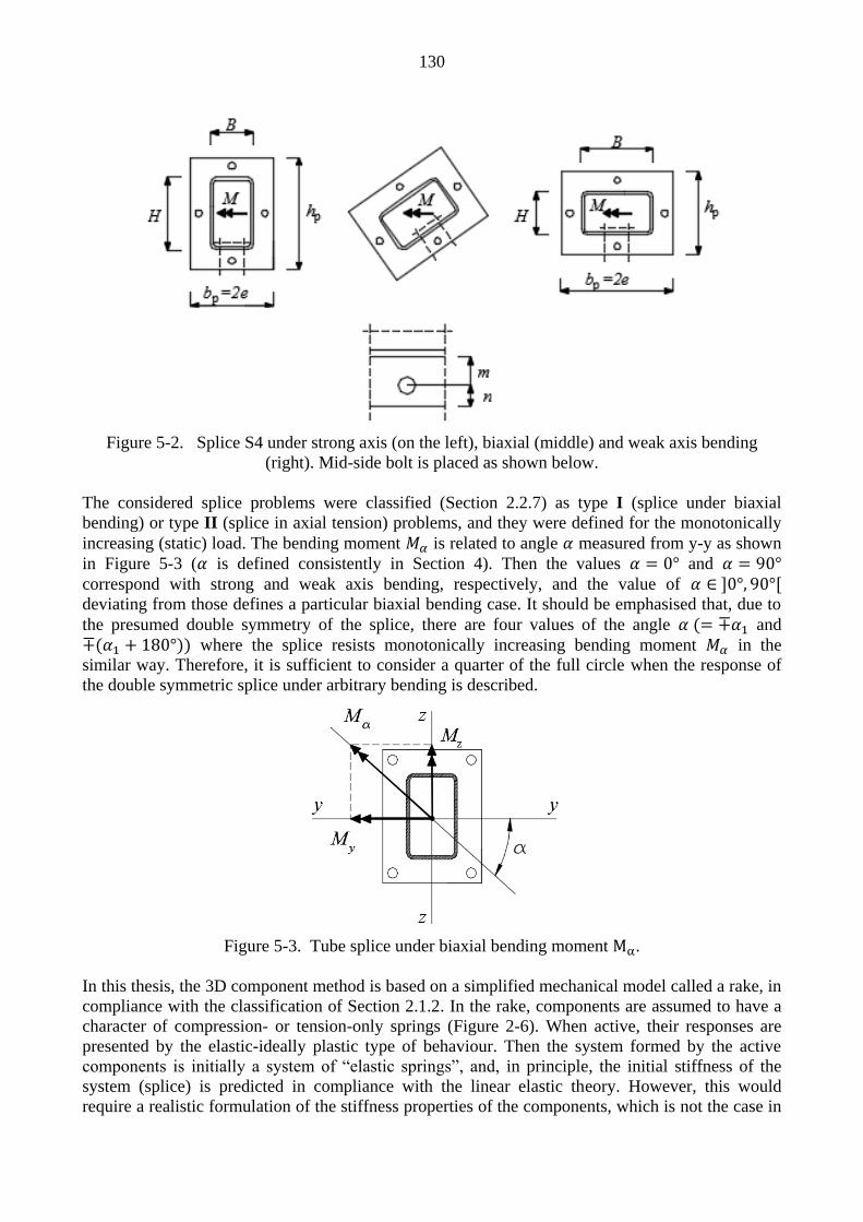
130

Figure 5-2. Splice S4 under strong axis (on the left), biaxial (middle) and weak axis bending

(right). Mid-side bolt is placed as shown below.

The considered splice problems were classified (Section 2.2.7) as type I (splice under biaxial

bending) or type II (splice in axial tension) problems, and they were defined for the monotonically

increasing (static) load. The bending moment is related to angle measured from y-y as shown

in Figure 5-3 ( is defined consistently in Section 4). Then the values and

correspond with strong and weak axis bending, respectively, and the value of

deviating from those defines a particular biaxial bending case. It should be emphasised that, due to

the presumed double symmetry of the splice, there are four values of the angle and

where the splice resists monotonically increasing bending moment in the

similar way. Therefore, it is sufficient to consider a quarter of the full circle when the response of

the double symmetric splice under arbitrary bending is described.

Figure 5-3. Tube splice under biaxial bending moment .

In this thesis, the 3D component method is based on a simplified mechanical model called a rake, in

compliance with the classification of Section 2.1.2. In the rake, components are assumed to have a

character of compression- or tension-only springs (Figure 2-6). When active, their responses are

presented by the elastic-ideally plastic type of behaviour. Then the system formed by the active

components is initially a system of “elastic springs”, and, in principle, the initial stiffness of the

system (splice) is predicted in compliance with the linear elastic theory. However, this would

require a realistic formulation of the stiffness properties of the components, which is not the case in

131

the prevailing component method in EC3 used as the starting point in this study. On the other hand,

the resistance of a single basic component is determined according to its ideally plastic response.

Every new component that has reached the plastic limit is the reason for the decreasing stiffness and

possibly to failure of the whole system. The latter can happen, when all components yield, or

through the loss of stability of the spring system because of the insufficient support by those

components in the elastic range that could still carry a larger load themselves. In any case, the

resistance of the joint can be attained by the simple rake. The principal objective is to study if the

bending resistance of the considered splices under biaxial bending can be predicted in the

satisfactory way by the rake defined consistently with the component method of EC3. Next, tension

and compression components are suggested for the 3D rake representing the tube splice, such that

they are defined in compliance with the ideas of the component method introduced in the prevailing

EC3; that is, this standard has been taken as the starting point for the component modelling. The

main interest is in the resistances of the tension components, which are based on the T-stub analogy

and the plasticity theory principles. In the rakes, the approximate stiffness values, called here

tentative stiffnesses were used for the components. In order to shed light on the used stiffness

model, these tentative stiffnesses are compared with the FE analysis results on splices in axial

tension as presented in appendix A5. It is that the responses of the individual tension components

then are considered directly (not in the joint level).

In order to replace a joint with a mechanical model equipped with components, in general, the

components must first be identified, and, moreover, their deformability curves must be determined.

The response of the joint can then be described more or less realistically depending on the

correctness of the deformability curves. The measured response of a component would allow the

fitting of the deformation curve directly to the test results, which is, unfortunately, difficult in

practise. If the deformability curve is constructed by theoretical means, it should be validated

against the tests. In this study, no experimental validation data were known at the “component

level”. Instead, available data was obtained by the bending test on the modelled splices or were

related to the material properties of the splice parts. The latter ones had been used in the estimation

of the properties of the suggested components. The validity of the 3D model was investigated at the

“joint level” based on the arranged tests on the tubes splices. Moreover, the experimental data was

enlarged through the numerical analyses supported by the tests. The splice tests and their results are

described in Section 3 while the numerical models are introduced in Section 4. The moment-

moment interaction curves (for the splices under bending in the arbitrary direction) were obtained

numerically supported by the tests as presented in Section 4.5.2. Finally, the failure curves of the

3D component method are compared with those numerically enlarged ones in Section 5.6.

5.2 Components in strong axis bending of a tube splice

In this thesis, the development of the three-dimensional component method is seen as an expansion

of the (in-plane) component method introduced in EC3 (EN1993-1-8, 2005). In order to model and

analyse the splices representing the driving examples of the thesis (S1 to S4) by the component

method, the steps over the application area of the standard must be taken. The structural features of

the considered splices not included in the standard are explained in Section 2.2.4.

For the analysis of a joint by the component method, the potentially relevant components must be

identified first. The response of the joint is described through the components activated by the

loading. The other potential components, which remain passive during the loading, are neglected in

the analysis. Next, the rectangular tube splice under strong axis bending illustrated by Figure 5-4a is

kept as a starting point with which the concepts and formulations of the standard are utilised when

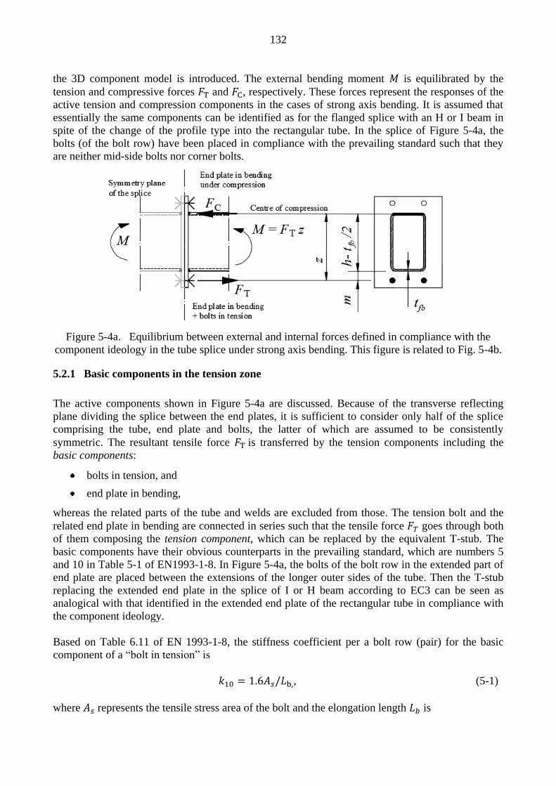
132

the 3D component model is introduced. The external bending moment is equilibrated by the

tension and compressive forces and , respectively. These forces represent the responses of the

active tension and compression components in the cases of strong axis bending. It is assumed that

essentially the same components can be identified as for the flanged splice with an H or I beam in

spite of the change of the profile type into the rectangular tube. In the splice of Figure 5-4a, the

bolts (of the bolt row) have been placed in compliance with the prevailing standard such that they

are neither mid-side bolts nor corner bolts.

Figure 5-4a. Equilibrium between external and internal forces defined in compliance with the

component ideology in the tube splice under strong axis bending. This figure is related to Fig. 5-4b.

5.2.1 Basic components in the tension zone

The active components shown in Figure 5-4a are discussed. Because of the transverse reflecting

plane dividing the splice between the end plates, it is sufficient to consider only half of the splice

comprising the tube, end plate and bolts, the latter of which are assumed to be consistently

symmetric. The resultant tensile force is transferred by the tension components including the

basic components:

bolts in tension, and

end plate in bending,

whereas the related parts of the tube and welds are excluded from those. The tension bolt and the

related end plate in bending are connected in series such that the tensile force goes through both

of them composing the tension component, which can be replaced by the equivalent T-stub. The

basic components have their obvious counterparts in the prevailing standard, which are numbers 5

and 10 in Table 5-1 of EN1993-1-8. In Figure 5-4a, the bolts of the bolt row in the extended part of

end plate are placed between the extensions of the longer outer sides of the tube. Then the T-stub

replacing the extended end plate in the splice of I or H beam according to EC3 can be seen as

analogical with that identified in the extended end plate of the rectangular tube in compliance with

the component ideology.

Based on Table 6.11 of EN 1993-1-8, the stiffness coefficient per a bolt row (pair) for the basic

component of a “bolt in tension” is

, (5-1)

where represents the tensile stress area of the bolt and the elongation length is

133

(5-2)

where and are the end plate thickness and height of the washer, respectively. Half of the

average height of the bolt head ( and nut ( ) is included in . It is noted that the average value

was consistently used as the height of the bolt head in the symmetric bolt models

(Section 4.2.2). If only another half of the splice is analysed, when the splice is understand as

divided by the rigid plane at mid span, should be replaced by = in order to obtain

physically right stiffness coefficient. The value of 1.6 for the coefficient of Eq. (5-1) is relevant in

the case of the bolted flange under prying. If the prying action is not present, the value of 2.0 should

be used. The tension resistance of an individual bolt is (Table 3.4 of EN 1993-1-8)

, (5-3)

where is the tensile stress area of the bolt and is the ultimate strength obtained in the tensile

test. The coefficient is taken as 0.9 for normal bolts, and the partial safety factor is replaced

by the value of 1.0 in order to obtain direct comparability with the test results.

The resistance of the end plate in tension is embedded in the procedure in which the resistance of

the equivalent T-stub comprising the end plate(s) and the associated connectors is determined. Then

the limit mechanism includes the yielding end plate and/or the yielding bolts. If the bolts are placed

as in Figure 5-4a, the stiffness coefficient for an “end plate in bending” defined per a bolt-row can

be estimated as (Table 6.11 of EN1993-1-8)

(5-4)

where is the effective length of the equivalent T-stub and and are, respectively, the

thickness of the end plate and the distance between the lower tube edge and the centre of the bolt in

the flange. By connecting the basic components in series, the tension component is formed. Its

position is defined according to the level of the bolt row in the two-dimensional splice model. The

stiffness coefficient of the component is obtained by the formula

. (5-5)

The physical stiffnesses are obtained by multiplying the stiffness coefficients ( , ) by the

associated values of Young’s modulus ( N/mm2). The resistance of the tension

component is determined through the procedure known as the “T-stub analogy”. The equivalent T-

stub is defined in EC3 such that “the design resistance and failure mode of an end-plate in bending,

together with the associated bolts in tension, should be taken as similar to those of an equivalent T-

stub flange”. The resistance of the equivalent T-stub is obtained according to Table 6.2 of

EN 1993-1-8 such that it is associated with the failure mode ( 1,2,3) giving the smallest value.

The failure modes of the T-stub are also described in Section 2.1.3. The value of the effective length

can be found as the minimum value related to the given yield line patterns suggested for the

extended end plates. The yield mechanisms, which are taken into account with splices S1 to S4, are

discussed in Sections 5.3 and 5.4. Although these mechanisms or their use are formally outside the

direct guidance given in the standard, they can be adopted to the 3D component analysis in

compliance with the ideology of the component method.

134

5.2.2 Basic components in the compression zone

The compression component must transfer the compressive resultant force due to

bending over the splice. The compressive force must go through the contact between the end plates

pushing each other in the compressive zone. In the spliced beam, the relevant basic component is

beam flange and web in compression (number 7 in Table 6.1 of EN1993-1-8).

This component is a part of the beam rather than belonging to the splice itself. According to the

standard (note 4 of Table 6.11 of EN1993-1-8), its stiffness coefficient ( ) should be taken as

equal to infinity and does not need to be taken into account when the rotational stiffness of the

splice is calculated. If the resistance of the beam in the compression zone is sufficiently large such

that failure in the tension zone determines the bending resistance of the splice, then the position of

the centre of compression is adequate data such that the bending resistance can be calculated as

, where and are, respectively, the resistances of the tension component and

lever arm in bending. A solution is obtained when the compressive resultant force is assumed to act

at the level of the mid-thickness of the compression flange (Figure 5-4a). In any case, the

compressive force must be transferred over the splice by contact between the end plates. The

associated basic component could be called the “end plate in contact in the compression zone”,

which is not presented in the standard. The physically nearest counterparts to it would be

represented by the combination of the two basic components, which are the “base plate in bending

under compression” (number 14 in Table 6-1 of EN1993-1-8) and “concrete in compression”

(number 13 in Table 6.1 of EN1993-1-8). The compressive component then is transferred through

contacts between the steel plate and concrete in the base plate joint, whereas in the considered

splice, contacts are formed between two steel plates.

5.2.3 Bending of the splice

In the standard, the component model of an end plated H and I beam splice under strong axis

bending is described, as in the case of beam-to-column joint when those parts of the component

model that are related to the column are neglected. It is assumed that the splice of a rectangular tube

can be treated in an analogical way with the splices of the H and I beams according to the

component ideology. Then the design resistance for the “beam flange and web in compression” can

be approximated by

, (5-6)

corresponding to Eq. (6.21) of the standard. In Eq. (5-6), is the design resistance of the

cross-section, is the height of the tube and is the thickness of the tube wall, which is usually

the same for the web and flange opposite to those in the H and I beams. If the plastic capacity of the

beam can be fully utilised (class 1), represents the plastic resistance of the tube ,

where is the plastic section modulus and is the yield strength. All considered splices had

smaller bending resistances than the tubes, such that the beam had no role in failure. The factors

affecting the rotational stiffness of the tube splices are the stiffnesses of the tension components and

the internal lever arm in bending, the latter of which can be approximated by

, (5-7)

in compliance with Figure 6-4a. The design moment resistance of the splice is

135

, (5-8)

where is the resistance of the equivalent T-stub. According to the standard, moreover, the

(secant) rotational stiffness of the splice depends on the stiffness of the T-stub obtained by Eq.

(5-5), such that

. (5-9)

The coefficient , being the divisor on the right side of the equation, is defined such that the change

in the stiffness from its initial value to the onset of the yield plateau occurs continuously in the

interval ] (Section 6.3 of EN1993-1-8).

In all bending tests on splices S1 to S4, it was used the same rectangular tube CFRHS 250x150x10

belonging to class 1 according to the cross-section classification of EC3. The yield moment of the

tube is , where is the elastic section modulus and is the

yield strength (Section 3). In strong and weak axis bending, it holds that m and

, respectively. For (biaxial) bending in the arbitrary direction

belonging to the first coordinate quarter, the yield moment is between those obtained in the weak

and strong axis bending, or . In the arranged tests, the largest registered

value of the bending moment was in biaxial test TE3 ( ), which is about 58% of the

yield moment in weak axis bending ( ). Thus, the tube remained in the elastic range in all

tests. In fact, the yield moment of the tube would very probably not be exceeded in any given

direction in which a similar bending test would be arranged. The plastic resistances

of the tube are about and in strong and weak axis bending, respectively. The

resistance of the “beam flange in compression” ( ) is definitely large enough not to be

reached in any considered tube splice.

The permanent deformations were concentrated on the splices, whereas the tube, and consequently

the welds, remains in the elastic range. The used welds, with matching or over matching filler metal

to the tube, satisfy the requirement of EC3 (6.2.3 (4) of EN1993-1-8), according to which the design

moment resistance of the joint ( ) should be “always limited by the design resistances of its

other basic components, and not by the design resistance of the welds”. This is supported by the

observations that any failure of the weld was observed in the tests. It should be noted that although

the welds themselves remained unbroken, the cracks were formed in the end plates near the weld

toes in the tests with flexible end plates. These cracks were perpendicular to the plate, and they

appeared clearly after the knee point (in the splice response) only in the strongly bent end plate,

such that the radius of bending clearly had the smallest values in the related “critical places”.

Perhaps the welding had weakened the end plate material near the weld (in HAZ) so that the

appearances of the associated cracks were more probable and occurred earlier than expected in the

plate without the weld. In any case, the influence of the welding was not taken into account in

component analysis because of its character as a secondary phenomenon obeying the usual

procedure suggested in the standard. In general, the proper welds guarantee the response of the T-

stubs such that the failure modes of EC3 can be used ( o Coelho et al 2004).

136

5.2.4 2D rake

A simplified mechanical model of the (half) splice of Figure 5-4a is shown in Figure 5-4b. The

considered splice under strong axis bending is presented as a 2D rake, where a rigid bar connects

the tension and compression components. The almost compressible compression component is

replaced by a support and the tension component is described as a spring with the elastic-ideally

plastic deformability curve. The stiffness and resistance of the tension component

are the decisive properties, which determine the response of the model in addition to the internal

lever arm obtained through Eq. (5-7). Let the be the extension of the tension component due

to the tensile force of the couple equilibrating the external bending moment

. The rotation of the (half) splice is , which depends on the stiffness of the tension

component . The stiffness coefficient is obtained through Eq. (5-5) based on the assumption

that the end plate (in bending) and the bolts (in tension) are connected as series.

According to the 2D model in the figure, the moment depends linearly on the rotation such

that as far as the tension component remains in the elastic range. The

plastic resistance of the splice is , where and are the resistance of the

tension component and the internal lever arm, respectively. The plastic resistance is

independent of the (initial) stiffness of the splice as demonstrated by Figure 5-4b on the

right. Consequently, the stiffness of the tension component ( ) can be replaced by an arbitrary

stiffness in the case of this simple model when the resistance is evaluated. In theory, the stiffness

values of a rake can be chosen freely on condition that the model can reach the full plastic

resistance such that all the components yield. Then the sufficient ability of the first yielding

components to tolerate plastic deformations without failure is required. Despite the sufficient

ductility of the components, the rake can lose its load carrying capacity before every component of

the rake has been reached its plastic resistance (Section 2.2.2). Provided that the determinate

(plastic) mechanism, which comprises the yielding components and those yet in the elastic range,

do not change because of the varying stiffnesses, these stiffnesses can be chosen freely and,

theoretically, even put these infinite at the limit when the resistance is evaluated. It is assumed then

that the elastic work done in the not yet yielding components can be neglected in respect to the

plastic work done in the (unrestrictedly) yielding ones.

Figure 5-4b. Two-dimensional rake for a splice shown in Figure 6-4a and its - curves. The

resistance is constant independent of the stiffness ( , when .

137

5.3 T-stub analogy

In the component method, the resistances of the extended end plate connections in the tension zone

are modelled by the T-stub analogy. Next, the procedure, where a bolted end plate is replaced by an

equivalent T-stub in tension, is discussed. This replacement is based on the analogy between the

plastic mechanisms in the actual component and in the T-stub such that the resistances of the bent

end plate and the flanges of the T-stub can be described by the yield line theory. The resistance is a

monotonically increasing function on the effective length in the associated failure mode. Then the

effective length related to a certain mode can be minimised instead of the collapse load itself. The

plastic mechanism that gives the smallest effective length is the determinate one. In this mind, the

procedure based on the effective lengths can be done in compliance with the upper bound theorem

of the plasticity theory. It is reminded that the determining mechanism and mode are eventually

known only after the resistances of all modes have been compared with each other.

5.3.1 Yield line analysis

The resistances of the tension components are approximated by the procedure based on the upper

bound theorem of the plasticity theory (Chen et al. 1988; Bower, 2012). For any chosen

kinematically admissible velocity field related to the certain yield mechanism, the collapse load can

be solved and compared with the others in order to find for the smallest one. The latter represents

only an approximate resistance unless the actual mechanism is guessed (i.e., if it belongs to the “set

of the chosen mechanisms”). This method is evidently “inherently unsafe” since it usually

overestimates the resistance. However, it is possible to describe the reasonable plastic mechanisms

for many problems and, consequently, obtain tolerable or even a good estimates from the practical

point of view. On the other hand, when the resistances are based on the knee point (plastic) strength

of the structure before the strain hardening stage, the upper bound theorems can offer resistances

clearly on the safe side, which has been exploited in the component method (Feldmann et al, 1996).

It should be noted that although the upper bound theorem of plastic collapse can be strictly proved

in the case of the rigid-ideally plastic response, it is generally utilised with the elastic-ideally plastic

structures, such that the elastic deformations and the associated elastic energy are neglected. This is

plausible when the elastic deformations remain small in comparison with the plastic ones, in which

case the internal dissipation related to the plastic work is approximately equal to the work done by

the external forces.

Plastic mechanisms, which comprise yield line patterns for the “end plate in bending” and/or

yielding of the “bolt(s) in tension” are considered in the tension zone of the tube splice under strong

axis bending. The associated tension components are defined per a bolt row (bolt pair) in a tension

flange as in the standard. It is assumed that the tensile force is perpendicular to the end plate and

moves in the direction of the force with the displacement in the virtual mechanism . Then the

external virtual work is

, (5-10)

whilst the internal virtual work can be expressed as

. (5-11)

where the first terms represent the work done by the plastic moment resistance of the plate

defined per unit length in the yield line with length , and where is the relative rotation

138

between the adjacent plate parts. In the second terms, the plastic resistance of the bolt (if

reached) is multiplied by the related elongation . For homogenous steel plates with symmetric

stress-strain behaviour in respect to tension and compression, it holds that

. (5-12)

where and are, respectively, the yield stress and thickness of the plate. It does not matter

then whether the upper or lower side of the plate is in tension in the yield line. By solving from

the virtual work equation

, (5-13)

an upper limit of the plastic collapse load for the associated mechanism is achieved. In line with

the ideology of the component method, a yield mechanism must be of local type such that it can be

defined as independently of the global behaviour of the joint. If a mechanism cannot be defined for

a bolt, it must be described as a “unified mechanism” for the associated group of bolts.

5.3.2 Procedure and examples

In order to determine the resistance of the tension component in the case of tube splice shown in

Figure 5-4a (or 5-4b), it is required that the resistance of the actual tension component

must equal the resistance of the equivalent T-stub, or

(5-14)

in modes and . The effective length of the equivalent T-stub can be solved through

Eq. (5-14) to which should be introduced a set of “reasonable mechanisms” in the associated mode.

The effective length is relevant only in modes 1 and 2, where the yiedl lines are formed. When the

minumum values of ( ) are known, the corresponding minimum values for the

resistances and are simply the resistances of the equivalent T-stub in modes 1

and 2 (Table 6.2 of EN1993-1-8). In mode 3, the tension reistance is attaned as the sum

of the resistances of the bolts. The tension resistance of the component is obtained finally as

(5-15)

in the case of the end plated splice. The failure mode giving the smallests resistance value is the

decisive failure mode. The similar procedure will be used also with the new components introduced

in this thesis. The essential requirement is that the effective lenght has been evaluated in a

reasonable way.

First, a plastic mechanisms of EC3, later labelled as number 1 in modes 1 and 2 (Table 5-1), are

considered as an example. In addition to these two modes, the one representing mode 3 and,

moreover, the mode without prying are shown in Figure 5-5. Based on the principle of the virtual

work presented by Eq. (5-13), the resistance of the actual component in mode 1 defined for the

tension flange (bolt row) can be solved as

, (5-16)

139

whilst the corresponding resistance of the equivalent T-stub is (Table 6.2 of EN1993-1-8)

. (5-17)

Figure 5-5. The plastic mechanisms in the bolted end plate are shown in the tension zone of the

tube splice under strong axis bending with the related T-stub.

By demanding that in compliance with Eq. (5-14), the effective length can be solved in

mode 1, which gives the result . For mode 2, correspondingly, it can be written as

(5-18)

where the terms including the bolt force (in yielding) will overturn each other. As a result, the

effective length is . Thus, it holds now that , the result of which

cannot be generalised. For the mode without prying (lowest in Figure 5-5), it is required that

, (5-19)

which leads, again, to the same effective length ( as in modes 1 and 2. Then only one

effective length is required for these three modes. It should be noted that the tension resistance

in the mode without prying (Table 6.2 of EN1993-1-8) usually is irrelevant with the beam

splices. However, the difference between the plastic mechanism in mode 2 and in the mode without

140

prying is only in the contribution of the yielding bolts. This similarity between the two different

modes can be utilised when the effective lengths are derived for mode 2. In general, the inequality

of the effective lengths determined for the equivalent T-stub in modes 1 and 2 will be taken into

account. In mode 3, there are no prying action and no yield lines in the end plate such that the

resistance of the bolted end plate equals the resistance of the bolts. Finally, the tension resistance of

the component is obtained through (5-15).

In Figure 5-6, another example on T-stub analogy is shown such that three possible plastic

mechanisms in the tension zone of the splice under strong axis bending are on the left side, and the

associated mechanisms of the equivalent T-stubs are beside them on the right side. In the considerd

example, there are corner bolts in the end plate, which will be discussed more comprehensive in

Section 5.3.4 below. It is noted here that the plastic mechanisms in modes 1 and 2, which are drawn

in Figure 5-6, represent the case number 10 in Figure 5-10. By the figure, the connection between

the actual component and the equivalent T-stub is demonstrated in failure modes 1 to 3. An inclined

yield line touching the tube corner appears in both failure modes 1 and 2 with prying action. In

mode 1, which corresponds to “complete yielding of the flange” with fully developed prying with

prying force , another yield line goes through the bolt hole, and no yielding of the bolts is

required for the mechanism. In mode 2, the bolt yields at the same time as the flange in the plastic

mechanism such that the prying force formally belongs to open interval [. The bolt

failure dictates the behaviour of the splice in mode 3 in which case, there are no prying effect

( ) and the yield lines of the end plate do not play any role.

Figure 5-6. Plastic mechanisms relevant for strong axis bending in the bolted end plate in the

equivalent T-stub are shown in failure modes 1 to 3. The dashed yield lines refer to the upper side in

tension whereas continuous lines refer to the lower side in tension.

141

5.3.3 Modified EC3 yield patterns

The plastic collapse mechanisms of the T-stub are classified (Zoetemeijer 1974) as those, where

bolt failure is decisive and those, where the collapse is due to the spreading plastic deformations

(yield lines) in the flange. The first involve cases with yielding bolts ( ) and without the fully

developed prying force belonging to a semi-open interval, or . In addition to the

yielding bolts ( ), the additional yield line going through the bolt holes are formed in the

limiting case when . In the second type of collapse, flexible flange yields alone with

mechanism comprising yield lines both in the bolt line and near the tension bar ( ) whilst

the bolt remains in the elastic range ). Although the division into failure modes used by

Zoetemeijer is slightly different than the classification introduced in EC3, the described behaviour

of the T-stub in tension is the same independently of the used formalism. Zoetemeijer investigated

the column flanges through the tests with specimens illustrated by Figure 5-7. The specimen is

pulled by the force such that the force must go through each flange connected by two bolts.

Because of the larger stiffness of the outer flanges in the specimen, they remain in the passive role

in the connections, and, consequently, the possible plastic collapse mechanism is formed by the

column flange and/or the related bolts. Zoetemeijer presented a formulation, where the column

flanges can be replaced by the equivalent T-stubs based on the concept of the effective length. This

formulation presented in 1974 is fundamentally similar to the that used in procedure based on the

equivalent T-stub in the component method of EC3.

Figure 5-7. Illustration of the plastic mechanisms introduced by Zoetemeijer for the column flange

in order to determine its effective length of the T-stub replacing the column flange.

The plastic mechanisms, which Zoetemeijer originally studied, are shown in Figure 5-7 as cases

with and without yielding bolts. In the mechanism on the left side, the contribution of the plastic

work done in the yield lines in the flange is added to the internal dissipation of energy done by the

142

bolt forces ( ). In the mechanism on the right side, in turn, the internal dissipation of the

energy is wholly due to the plastic work done in the yield lines. In this latter case, the yield line

pattern includes yield lines, which can be intuitively associated with the plastic hinge in T-stub in

mode 1 of EC3 coinciding with the bolt line (Figure 2-4 or 5-6). Based on the equality of the

internal dissipation of energy with the work done by the external load, Zoetemeijer derived the

equilibrium equations for the minimum collapse loads. Furthermore, he modified these formulations

by replacing them with approximate but simpler (or more practical) ones. By requiring that the

failure modes and resistances of the column flange and the “equivalent T-stub” are the same, the

effective lengths of the T-stubs can be determined. In general, the mechanisms representing the

different failure modes have the different effective lengths. As said above, Zoetemeijer modified

these equations, which intended for the design purposes, by introducing the same effective length to

both cases (with and without yielding bolts). It should be noted that, when collapse of the

mechanism is based solely on the spreading plastic deformations in the column flange, the influence

of the prying effect was taken into account through the equilibrium analysis through the mechanism

shown at the bottom of Figure 5-7.

The tension components needed in the analysis of the considered splices with the corner and mid-

side bolts, are formally outside the application area of the component method of EC3. However,

some yield line patterns of the standard can be utilised as modified when the smallest effective

length is sought for the equivalent T-stub. The modified formulas are shown in Table 5-1 based on

“effective lengths for an end plate” introduced in Table 6.6 of EN1993-1-8. These formulas are

presented separately for splices with corner bolts (S1 to S3) and mid-side bolts (S4) and they are

numbered from 1 to 7 such that numbers 1 to 4 correspond to the non-circular yield line patterns

(with prying) and 5 to 7 correspond to the circular ones. It should be noted that the additional yield

line patterns suggested later are numbered from 8 to 10. All formulas are written in the form that is

in compliance with the geometry shown in Figure 5-8 for the symmetrically placed corner bolts and

for the mid-side bolts using the dimensions , and of the figure. In general, the interpretation of

(edge) distances and depends on the loading case, but because of the symmetry ( ), it has

no significance for the associated corner in the tension zone. In the case of a bolt row, the mutual

distance between the centre lines of the bolts is marked by In addition, the width of the end plate

is defined in compliance with Figures 5-1 and 5-2 depending on the directions of the applied

resultant bending moment such that the bolts of the bolt row in question should be part of the same

plastic mechanism in the tension flange. When the tension component related to the mid-side bolt is

considered, number 3 can be interpreted as “one-sided pattern” with (Figure 5-9 on the

left), and those formulas including are omitted. In Table 5-1, the index of the effective length

refers to the failure mode, which is either 1 (yielding flange) or 2 (bolt and end plate yield at

the same time). There are no yield lines in the plastic mechanism if failure mode 3 of the equivalent

T-stub prevails, and, consequently, no yield patterns are required. This happens only when the end

plate is thick enough in respect to the end plate.

Corner bolts. The patterns of Table 5-1 are discussed when employed in the case of the corner

bolts. As explained above, the formulas suggested here for the bolts placed in the corner areas are

modified from those suggested in the standard (Table 6.6 of EN1993-1-8). The yield line patterns

numbered 1 are illustrated by Figure 5-9 in modes 1 and 2. In failure mode 1, a yield line goes

near the tube and another yield line coincide with the line of the bolts whilst the bolts themselves do

not yield. In mode 2, only the yield line near the tube appears, while the bolts also yield. These

modes have their direct counterparts in the yielding T-stub (as demonstrated by Figure 5-6) and,

thus, the analogy between the extended end plate flange and the T-stub is obvious. In mode 1, the

plastic dissipation comes only from the deformations (rotations) in the yield lines whilst the (elastic)

143

work done by the bolt force and prying force is neglected in the energy equation. It should be noted

that the effective lengths in both modes are equal ( ), which holds with all cases

included in Table 5-1.

Figure 5-8. End plate flanges with the symmetrically placed corner bolts on the left (S1 to S3) and

mid-side bolts on the right (S4) in regard to the associated symmetry lines L-L.

Figure 5-9. A simple collapse mechanisms (number 1 in modes 1 and 2, Table 6-1) for the flange

of the end plated connection corresponding the modes of T-stub according to classification of EC 3.

The formula numbered with 4 is based directly on those derived by Zoetemeijer and the associated

yield line patterns are illustrated by Figure 5-5. As explained above, though the effective lengths

originally are unequal in modes 1 and 2, they are set to be equal in the design formulas. Number 4 is

obviously rare when the bolts are relatively far apart. The formulas numbered 2 and 3 can be

obtained from formula number 4 by intuitive reasoning. The effective length of for pattern

number 3 is obtained when the distance of between the bolts is replaced by , where is

interpreted as the length of the yield line measured from the bolt centre to the side of the end plate.

There are two separate plastic mechanisms with unconnected yield patterns in the end plate in

pattern number 3. It might be decisive in the case of large distance ( ) between the bolts and the

small side distance ( ). In formula number 3, the effective length depends on the

distances defined in a corner rather than in a flange. Consequently, it can be understand as a “corner

mechanism” in its character. The effective lengths for pattern number 2 correspond to the

case in which the distance between the bolts ( ) is set to disappear such that the pattern is reduced

around a bolt. When defined for a flange, two separate patterns are formed around both corner bolts.

Because the formulas of Table 5-1 are defined per a tension flange, the remaining terms in the

formula for pattern 4 had to be multiplied by two so that they would stand for two separate “full

mechanisms”. Pattern 2 is, in principle, reasonable in the case of the relatively large mutual distance

between the bolts and the small distance to the edge of the end plate (when is small).

144

It should be emphasised that the smallest of the effective lengths related to the non-circular patterns

1 to 4 must be selected as the determinate one, unless one of the circular patterns gives a lower

value. The circular patterns can be related only to mode 1 (complete yielding of the flange) or to the

mode without prying (omitted here). The circular patterns are numbered from 5 to 7 in Table 5-1. In

principle, they are assumed to arise only in mode 1 without prying, such that the patterns cannot

extend to the edges of the tension flange. Mechanisms 5 and 6 could be defined separately per a

single bolt, such that number 5 stands for a circle in the end plate about the bolt, whilst number 6

extends from the bolt, which is the centre of the semi-circular pattern, to the side of the end plate

with the straight yield lines of length . Moreover, “unified pattern” number 7, where two semi-

circular patterns are connected with the straight yield lines of length , is unlikely when the bolts

are relatively wide apart in the tension flange.

Mid-side bolts. The reasonable yield line pattern(s) are also required for the T-stub analogy used to

replace the actual components in the splice with the mid-side bolts, one in each end plate flange.

The potential patterns given on the right side in Table 5-1 are again modified from those given in

the Table 6.6 of the standard. Because there is one bolt instead of a pair of a bolts (bolt row) in the

flange in the case of four-bolt layout with the mid-side bolts, the effective lengths must be divided

by two although they are still defined per tension flange, whereas the formula dependent on

(distance between the bolts in pattern 4) can be dropped from the potential ones. The formulas for

patterns 1 and 3, including (width of the end plate) and , respectively, are not plausible

unless the end plate is quite narrow. In the case of the wider end plate flange with the mid-side bolt,

pattern 2 is the only modified EC3 mechanism, which is reasonable for the single mid-side bolt in a

(tension) flange. No particular yield line patterns will be suggested as related to the mid-side bolts.

Table 5-1. Effective lengths of the equivalent T-stubs based on EC3 formulations. They are related

to the symmetrically placed corner bolt and mid-side bolt shown in Figure 6-8 and they are defined

per a tension flange (including one or two bolts).

Remarks. As mentioned above, the patterns available in the standard are not originally intended for

the end plates with corner or mid-side bolts. As in the standard, these formulas are defined for a bolt

row (considered individually or as part of a group of bolt rows). In principle, there are no obstacles

to adopt them for end plates with the corner or mid-side bolts under the condition that the related

mechanisms are used when the minimum value for the limit load is sought through comparisons

between all admissible yield mechanisms. Moreover, they can be defined, formally, “per a single

EC3

modifications

Tension flange with the corner bolt

(defined for two bolts)

Tension flange with the mid-side

bolt (defined for one bolt)

Pattern Non-circular patterns

1

2

3

4

Pattern Circular patterns

5

6

7

145

nro. 8/Wald for mode 1 nro. 9/Laine for mode 1 nro. 10/Wheeler for mode 1

30°

30° xs

nro. 8/Wald for mode 2 nro. 9/Laine for mode 2 nro. 10/Wheeler for mode 2

30°

30° xs

bolt” as long as this does not cause a physically incorrect situation. This can occur, for example, if

the pattern connects two bolts to the same mechanism while one is in the compression zone. Of

course, these mechanisms may be less reasonable than those particularly intended for the corner

bolts or mid-side bolts. In any case, the aim is to determined the smallest value for the effective

length defining the equivalent T-stub. At least, this procedure stands for a well-organized approach

for the determination of the component resistance.

5.3.4 Particular mechanisms for the tension flange with the corner bolts

A yield line patterns intended for the analysis of the end plate connection with the corner bolts have

been discussed little in the literature on structural steel design. Examples on those articles, where

the “corner mechanisms” are discussed, has been mentioned already in Section 2 (Wheeler 1997b;

Wald et al. 2000; Laine 2007; Heinisuo et al. 2012). The particular yield line patterns used in this

thesis were named according to the researchers (Wald, Laine and Wheeler), who had utilised them

or very similar ones earlier in their studies. All these patterns are based on engineering intuition and

represent simple forms that can be used in hand calculations. The use of next suggested mechanisms

shown in Figure 5-10 is restricted in the case of the symmetrically placed corner bolt, i.e., the

symmetry is required in regard to line L-L, as shown in Figure 5-8. Although none of these

mechanisms would give the absolute minimum for the limit load, the smallest obtained one given

by these reasonable mechanisms is likely to be accurate enough for the practical design.

Figure 5-10. Corner mechanisms with prying in modes 1 and 2 in the tension zone of the tube

splice under strong axis bending. A dashed yield line is related to bending of the plate with tension

side up. Bolts are blackened when yielding.

The plastic yield line patterns of Figure 5-10 are numbered from 8 to 10, such that the preceding 7

patterns refer to those introduced in Table 5-1 above. It should be emphasized that a pair of

mechanisms is devoted to each number: one for mode 1 (complete yielding of the end plate) and

another for mode 2 (yielding of the bolt and end plate at the same time). The formulas of the

effective lengths of the equivalent T-stubs ( and ) are given to these six cases in Table

5-2. These formulas were derived earlier in a slightly different way in respect to the failure modes,

146

where the yield line mechanisms were divided into cases “with prying” (mode 1 with fully

developed prying) and “without prying” (Heinisuo et al 2012). When the end plate splices are

considered, the mode without prying is usually irrelevant. Instead, the plastic mechanisms represent

failure modes 1 and 2, both of which are formed under the influence of prying. Here, the effective

lengths are derived directly in modes 1 and 2 and confusion related to these modes is corrected.

Mechanism number 8 (Wald) is presented as a more detailed example, because it produces a simple

formulation by which the role of the yield line analysis as part of the derivation can easily be

elucidated. When the extended end plate flange belongs to the tension zone entirely, as in the figure,

it does not matter whether the corner components are defined for a bolt row (as in the standard) or

for an individual bolt. Mechanisms 8 and 9 of Figure 5-10 can be defined separately in the case of a

single corner in the tension zone, whereas mechanism 10 is relevant only when both corners are in

the tension zone. The yield line going “near the tube corner” is assumed to meet point O, where the

extensions of the straight parts of the outer edges of the tube profile intersect (Figure 5-8).

Furthermore, the diameter of the hole will not be reduced from the length of the associated yield

line “going through the bolt” following the procedure of EC3.

Number 8 (Wald). The two mechanisms representing modes 1 and 2, both of which are numbered

as 8, are obviously the simplest reasonable ones for the end plate with corner bolts. This mechanism

is referred to by the name of the professor František Wald from Prague. In mode 1, with fully

developed prying, the yield lines form the mechanism solely (the bolts do yield only in the limiting

case). In a corner, two parallel yield lines are perpendicular to the symmetry line L-L (Figure 5-9):

one of them goes through point O and another through the bolt. In mode 2, only the yield line going

through point O is formed in addition that the bolt yields (blackened in Figure 5-10). The condition

for the distance between the yield lines at the lower edge of the end plate must be fulfilled so

that the adjacent corner mechanisms will be acceptable in the tension flange. It should be noted that

the yield line going through a certain point in line L-L is shortest when it is perpendicular to this

line. This also minimises the plastic work in the yield line in respect to its direction. In this mind,

the minimisation of the limit load is included in the yield pattern in advance.

The mechanisms numbered as 8 in modes 1 and 2 is shown also in Figure 5-11, where the lengths

of the yield lines are given and displaced states are illustrated in a vertical section through line L-L,

such that another half of the splice is coloured grey in order to denote that only the half of the splice

is considered. For the plastic mechanism in mode 2, the external and internal virtual work are,

respectively, and . In the latter, the virtual rotation

in the yield line is expressed by the aid of the virtual displacement

representing the half of the distance between the end plates under the tubes. The principle of virtual

work gives the component resistance as

. (5-20)

On the other hand, the resistance of the equivalent T-stub in mode 2 is (Table 6.2 of EN1993-1-8)

= (2 . (5-21)

By assessing according to Eq. (5-14), the effective length can be solved as

. (5-22)

147

It is notable that the terms representing the work done by the bolts in Eq. (5-20) and (5-21) were

overturned in Eq. (5-22) such that this simple form for effective length could be obtained. Formally,

the same effective length can be derived by neglecting the (plastic) work done in the bolts in mode

2, which results in the analogue with the “mode without prying” when the yield lines are the same.

In mode 1, with complete yielding of the flange, the component resistance is

(5-23)

and the corresponding resistance of the T-stub can be written as

. (5-24)

It follows from requirement that

(5-25)

It should be emphasised that the effective lengths of the T-stubs and related to

modes 1 and 2, respectively, are unequal. It should be noted that the effective lengths for the

noncircular yield line patterns, which are given for the individual bolt row in the extended end plate

in Table 6.6 of EN1993-1-8, have the same value in modes 1 and 2. This approximation is based on

the simplified design formulas presented originally by Zoetemeijer (1974). The different effective

lengths in modes 1 and 2 must be taken into account when the corner components are embedded in

the procedure of the prevailing standard through T-stub analogy.

Figure 5-11. Mechanisms no. 8 in modes 1 and 2 for the corner component.

148

Number 9 (Laine). The next considered pair of plastic mechanisms is named after Mr. Ville Laine.

Based on the FE simulations, Laine (2008) has suggested that the angle between the yield lines and

the normal (vector) of the edge of the end plate should be (Figure 5-10). The yield lines from

point O (Figure 6-9) to the edges in modes 1 and 2, as well as two more yield lines from the bolt

hole to the edges in mode 1, have this attribute. In addition, one yield line coincides with the

symmetry line L-L in both modes. In mode 2, it extends from point O to the outermost corner of the

end plate, and in mode 1 from point O to the bolt. It is required that the yield lines of the patterns in

the adjacent corners do not intersect. The effective lengths of the equivalent T-stubs for mechanism

9 in modes 1 and 2 are

and , (5-26)

which can be obtained in a procedure similar to the one outlined in the case of mechanisms 8 in

modes 1 and 2. The exact formulas for the effective lengths are given in Table 5-2 below. Again,

unequal values for and arose. If mechanisms 8 and 9 are compared with each other in

mode 2, mechanism 8 always determines the collapse load, because of the inequality

. Depending on the values of and , the dominant mechanism in mode 1 is the

one with the smaller effective length. It is number 8 only if . The effective lengths for

plastic mechanisms, both of which are numbered by 9 in modes 1 and 2, are determined without

minimisation in respect to any variable defining the plastic behaviour.

Number 10 (Wheeler). The third pair in the considered set of plastic mechanisms for the extended

end plate flange in tension with symmetrically placed corner bolts was named after professor

Andrew Wheeler from Australia. The assumed yield line patterns can be seen as modified from

“yield line mechanism 3” suggested originally by Wheeler et al (1997b). The original mechanism is

shown on the left whereas the modified one (in mode 1) is shown on the right in Figure 5-12. The

original mechanism describes the behaviour of the whole splice under strong axis bending,

including a yield line in the compressive zone, whereas the modified mechanism (on the right) is

defined only in the tension zone. The latter is used in order to describe the resistance of the tension

component to which the equivalent T-stub analogy can be applied. In Wheeler’s mechanism, the

lines parallel to the yield lines in the tension zone and the third line, which coincide with the yield

line in the compressive zone, will intersect at the same point (P) in accordance with yield line

theory (Figure 5-12 on the left). Then a global mechanism of this kind is kinematically admissible.

In the modified mechanism, which is of the local type, point P is assumed to transfer very far such

that the yield line in the compression zone can no longer be in the end plate and yield lines in the

tension zone (at the same corner) are eventually parallel to each other, as shown in the figure on the

right. Moreover, angle correspondingly goes to zero at the limit, which represents an assumption

on the local mechanism in the tension zone. Such reasoning sheds light on the difference between

the global and local strategy in modelling, the latter of which represents the ideology of the

component method.

In the two mechanisms numbered 10 in Figure 5-10 for modes 1 and 2, the yield lines that go near

the lower tube corners intersect at a certain point, the distance of which from the lower edge of the

end plate is marked . This distance determines the yield line pattern unambiguously, and it can be

used as a variable in regard to which the collapse load of the mechanisms can be minimised. The

minimisation problem is defined in the semi-open interval , where and are as

shown in Figure 5-9. The mechanism in the lower limit of the interval resembles the one that

was called number 8, with , with the exception that the yield lines are not necessarily

perpendicular to the symmetry line of the corner (L-L). In that case, mechanism 8 ) would be

149

decisive. In the upper limit of the semi-open interval , the mechanism in mode 1

changes from admissible to non-admissible (because of the extra, vertical yield line in the middle of

the flange). It should also be noted that, by neglecting the vertical yield line and by setting the

inclined lines as horizontal, the “modified EC3 mechanism” numbered 1 is obtained. Intuitively,

mechanism 10 can be seen to represent the possible plastic behaviour between mechanisms 1 and 8.

The effective lengths of the equivalent T-stubs and in modes 1 and 2, respectively,

were obtained using a procedure outlined in the case of mechanism 8. The case without prying can

utilized alternatively. The effective lengths for all cases 8 to 10 are given in Table 5-2. For

mechanism 10, is written as a function of and , in turn, is presented as the

function of angle . Their smallest values are attained when or

. It is emphasized that there is an unambiguous relation between variables and . In Table 5-2,

the associated value of (mode 2) is expressed as dependent on the dimensions of the tension

flange defined in compliance with Figure 5-1. The minimum value of can be determined

numerically, based, for example, on the method of trial and error, as has been done in the case of

the considered splices in this work.

Figure 5-12. Wheeler’s original yield line pattern (global) and mechanism number 10 in mode 1

(local) defined in compliance with the “T-stub ideology” in the tension zone.

Table 5-2. Effective lengths for the corner mechanisms of Figure 5-10 in modes 1 and 2 for the

symmetrically placed corner bolts in compliance with Figures 5-1 and 5-9.

Pattern

Effective length of the equivalent T-stub

defined for a bottom flange and two bolts [mm]

Mode 2 (prying)

and mode without prying Mode 1 (fully developed prying)

Number 8

(Wald)

Number 9

(Laine)

Table 5-2 continues in the next page.

150

Remark. Three mechanisms (8 to 10 of Figure 5-10) were intended for the analysis of the tension

flanges with symmetrically placed corner bolts. Conversely to mechanism 10, which is reasonable

only when the whole flange is in tension, mechanisms 8 and 9 can be used for the “one corner only

in tension” independent of the adjacent corners. Thus, they can be used easily as tension

components in 3D analysis of the splices under arbitrary biaxial bending. If the bolts (bolt row) are

connected by the unified yield line pattern in the tension flange, as assumed with mechanism 10, the

analyst must check whether this really can happen in the considered case.

5.3.5 Decisive mechanisms

The effective length of the T-stub can be minimised in modes 1 and 2 instead of the limit load of the

decisive mechanism in compliance with the upper bound theorem. Thus, the decisive mechanism

stands for the effective lengths and in modes 1 and 2, respectively, such that

and , (5-27)

where and represent the effective lengths related to yield patterns and . In mode 1

both the non-circular and circular patterns should be included in the comparisons between the

modified mechanisms of EC3, whilst in mode 2, the circular patterns are not relevant. The particular

(corner) mechanisms in modes 1 and 2, should be included in the comparisons. The component

resistance can finally be obtained as the smallest collapse load through Eq. (5-15) in the comparison

between all modes (1, 2 and 3). Then the resistance of the component and the associated mode and

mechanism are solved at the same time.

5.4 Tension components of splices S1 to S4

The resistances (and stiffnesses) of the considered splices S1 to S4 depend decisively on the

properties of their tension components. These resistances can be determined through the T-stub

Number 10

(Wheeler)

The minimum is obtained when

Angle α should be defined such that the

minimum value for effective length is

obtained.

151

analogy based on the modified EC3 mechanisms and particular mechanism in the case of splices S1

to S3 with corner bolts. The modified EC3 mechanisms are only used for splice S4 with the mid-

side bolts. For convenience, the geometrical dimensions of the considered splices were gathered

from Sections 3 in Table 5-3. These dimensions are needed when the component properties are

determined for the 3D component analysis. For clarity, they are given separately in the case of

strong axis bending (= SAB) and weak axis bending (= WAB). In addition, the material properties

of the splice parts for the component analysis are shown later (Table 5-6).

Table 5-3. Dimensions of splices S1 to S4 are shown in compliance with Figures 5-1, 5-2 and 5-

9. In addition, is the diameter of the washer. The dimensions all are given in millimetres.

Splice

S1-S3, SAB 150 250 290 390 230 40 30 30 36

S1-S3, WAB 250 150 390 290 330 40 30 30 36

S4, SAB 150 250 290 390 -- 40 30 145 36

S4, WAB 250 150 390 290 -- 40 30 195 36

5.4.1 Effective lengths

The effective lengths of the equivalent T-stubs for the tension components of splices S1 to S4 were

determined according to the formulas of Tables 5-1 and 5-2. Their values are given to splices S1 to

S3 and for splice S4, respectively, in Tables 5-4 and 5-5, where they are presented separately in the

strong and weak axis bending cases (SAB and WAB, respectively). The only difference in geometry

between splices S1, S2 and S3 with the corner bolts is the thickness of the end plate. Consequently,

the effective length, which does not depend on the plate thickness, is determined in a similar way

for those three splices and has the same value for each of them. It should be noted that splice S4

with the mid-side bolts is the only one of its kind in the considered splices.

Those cells in Tables 5-4 and 5-5 that show the minimum effective length in modes 1 and 2 for the

tension component of splices S1 to S4 are surrounded by doubled borders in the case of strong and

weak axis bending. There are a total of eight minimum values for effective lengths in modes 1 and 2

for strong and weak axis bending. For splices with the corner bolts (S1 to S3), the smallest effective

length is obtained by the particular corner mechanisms numbered 9 (Laine) in mode 1 in weak and

strong axis bending. In mode 2, the modified EC3 mechanism numbered 3 is decisive in weak and

strong axis bending. This non-circular “standard mechanism” in question could also be classified as

a corner mechanism. Accordingly, the effective length of this mechanism depends only on the

distances from the centre of the bolt to the edges of the end plate ( and . For splice S4 under

strong and weak axis bending, the minimum values of the effective lengths in both modes 1 and 2

are obtained with the noncircular pattern numbered 2 as expected.

The values of the effective lengths, which are related to the circular yield line patterns (mode 1 with

complete yielding of the splice), were given in above tables, because any limits has not been

assessed for the associated formulas in the standard whether they are physically relevant or not. In

those, the radius of the circular part ( ) in the end plate should extend from the centre of the bolt

line to the bracing, which is represented by the outer edge of the tube profile (specifically, to the toe

of the weld). However, there is no room for the circular patterns to be wholly inside the flange

( ) either in the splices with corner bolts (S1 to S3) or in the case of the splice with the mid-

side bolts (S4).

152

The determining mechanisms for splices with the corner bolts (numbers 2 and 9) can be defined

separately for each bolt independently of neighbouring bolt. In the case of the mid-side bolts, on the

other hand, there was no difference regardless of whether the component is seen to represent a

single bolt or a tension flange. Thus, each possible mechanism with minimum effective length can

be defined for a separate bolt independently of neighbouring bolt. This is convenient for the 3D

model.

Table 5-4. Effective lengths for tension flanges of splices S1 to S3 under strong and weak axis

bending abbreviated as SAB and WAB, respectively.

Effective lengths for the flange

in millimetres [mm]

SAB WAB

Mode 1 Mode 2 Mode 1 Mode 2

Noncircular patterns (Table 6-1)

145.0 145.0 195.0 195.0

2: * 197.5 197.5 197.5 197.5

3: * 128.8 128.8 128.8 128.8

4: * + ** 213.8 213.8 263.8 263.8

Circular patterns (Table 6-1)

5: 251.3 ─ 251.3 ─

6: * 185.7 ─ 185.7 ─

7: ** 355.7 ─ 455.7 ─

Patterns for corner bolts (Table 6-2)

8 (Wald) 100.0 140.0 100.0 140.0

9 (Laine) 95.2 155.9 95.2 155.9

10 (Wheeler) ** 98.9 131.5 --- ---

* = For symmetric corners: .

** = Shared mechanisms with patterns including a bolt row.

Table 5-5. Effective lengths for the tension flange of S4 under strong and weak axis bending.

Effective lengths for the flange

in millimetres [mm]

SAB WAB

Mode 1 Mode 2 Mode 1 Mode 2

Noncircular patterns (Table 6-1)

1: 145.0 145.0 195.0 195.0

2: ( * 98.8 98.8 98.8 98.8

3: * + ** 121.9 121,9 146.9 146.9

Circular patterns (Table 6-1)

5: 125.7 ─ 125.7 ─

6: +2e)/2 ** 207.8 257.8

* = For mid-side bolts:

** = One-sided mechanism

153

5.4.2 Resistances and determining mechanisms

First, the strength properties of the end plates and bolts of the considered splices are presented and

discussed. Then the resistances and failure modes of tension components are determined.

.

End plates. For the end plates, the value of the yield strength ( ) is defined such that in

the analyses by the component method. The (plastic) resistance of the end plate in bending has an

important role in the behaviour of the tension components in modes 1 and 2. The plastic moment

defined per unit length for a plate can be evaluated through Eq. (5-12) based on the actual yield

strength and the measured end plate thickness . The associated values are shown in Table 5-6

in addition to the values of ultimate strength and the ratio for the end plates of

splices S1 to S4. The thickness of the end plate stands for the primary factor, which affects the

plastic moment of the end plate. The ratio describes the utilisation rate of the specimen in a

tension test at the moment when the (higher) yield stress is reached and the preceding yield plateau

and the strain hardening portion are still to come. In this case, the tensile test represents behaviour

typical for a specimen made of ductile, non alloyed steel. Although determines the ultimate

material strength only in the nominal mind, the quantity can be used as a

reference value when other types of structural behaviours are characterised. Then the value of

can be compared with the “relative reserve” of the structure, which is

determined according to and corresponding to the computational plastic limit load and actual

resistance, respectively. A relative reserve expected after the predicted resistance may be smaller or

larger than the tensile test specimen has. It is emphasized that a simple comparison like this

includes no direct data on the ductility of the structure, which would require a more comprehensive

procedure, where the ability of the structure to undergo large plastic deformations is taken into

account.

Table 5-6. Plastic moment resistances and the strength ratio for the end plates.

Splice

[mm]

[MN/m2

]

[kNm/m ]

[MN/m2

]

S1, S4 11.0 429 12.8 582 0.74

S2 15.0 378 21.3 532 0.71

S3 20.3 380 39.1 564 0.67

Bolts. The resistance of the “yielding bolt” is predicted in EC3 through Eq. (5-3), which, in the case

of the used M20 bolt, gives the value

250 kN

when is replaced by the measured average maximum tensile force of the

individual bolt (see Section 3.2.2); that is, it is replaced by the actual strength of the bolt. As

explained above, = 0.9 and the partial safety factor = 1. Here, the utilisation rate is

understood as the relation between the resistances predicted by the component method and the

actual resistance. The utilisation rate of the bolt is now defined formally by the ratio

154

which is clearly larger than the values of for the end plates given in Table 5-6. This is related to

the brittle character of the bolts (high-alloy-steel) when compared with the end plates with the

significant plateau and the related strain hardening phase (non-alloyed carbon steel). It is

emphasized that the bolt properties are described in accordance with the direct tests of the entire

bolts and the assumptions based on in the standard.

It is expected that in a mode 1 mechanism (yielding of the flange), the ductile character of the end

plate has an essential role in the splice behaviour, whilst in the case of mode 2 (yielding of the

flange and bolt failure), the less ductile behaviour is expected due to the increasing role of the bolts.

In the analyses by the component method, the partial safety factors are neglected (i.e., they are

assumed to be one), in order to make the results obtained by the component method directly

comparable to the measured (actual) behaviour.

Resistances and modes. When the minimum effective lengths have been determined in modes 1

and 2, the related resistances and of the equivalent T-stubs can be calculated (Table

6.2 of EN1993-1-7). If the dimension of the washer is taken into the account, the resistance in mode

1 according to the alternative method can be evaluated as

, (5-28)

where stand for a quarter of the diameter of the washer. Other symbols of Eq. (5-28)

have been explained above (Figures 5-1, 5-2 and 5-9) and their values can be found in Table 5-3. In

method 2, “the force applied to the T-stub flange by a bolt is assumed to be uniformly distributed

under the washer” (Note 2 in Table 6.2 of EN1993-1-8). As a consequence, a higher resistance is

obtained in mode 1 (yielding of the flange). The alternative method is relevant only with the end

plates flexible enough (splices S1 and S4) whilst in the case of stiffer end plates (splices S2 and S3),

this method should been abandoned. The resistance in mode 3 (bolt failure) must be

evaluated as the sum of the resistances of the associated bolts, or

. (5-29)

For the individual tension bolts, the resistance of was given above in this section. It should be

reminded that all considered splices had the bolts with the same size and grade.

The resistance of the tension component can be obtained, finally, as a part of seeking for the

smallest limit load, through the comparison in accordance

with Eq. (5-15). In Table 5-7, the values of the resistances of the tension components ,

and in modes 1, 2 and 3, respectively, are shown for splices S1 to S4. In addition, the

determining mode and mechanism are shown. The mode 3 (bolt failure) is not decisive in any case.

For splices S1 and S2, the particular corner mechanism numbered 9 (Laine) in mode 1 was

determinate, whilst for splice S3, with the thickest end plate ( ), the standard

mechanism numbered 3 in mode 2 gave the smallest resistance. The modified EC3 pattern

numbered 2 was the determining one for splice S4 with the thin end plate due to the higher

stiffness of the splice related to the mid-side bolts.

155

Table 5-7. Resistances calculated based on the equivalent T-stub. The values are defined per

tension flange (i.e., per two corner bolts (S1 to S3) or per a mid-side bolt (S4)).

Splice

[kN]

[kN]

[kN]

=

[kN]

Determining

mechanism

S1, method 1* 124 262 500 124 No. 9 mode 1

S1, method 2 155 262 500 155 No. 9 mode 1

S2 202 292 500 202 No. 9 mode 1

S3 373 358 500 358 No. 3 mode 2

S4, method 1* 128 144 250 128 No. 2 mode 1

S4, method 2 161 144 250 144 No. 2 mode 2

* = Neglected in the case of 10 mm end plates.

Although the alternative method (method 2) was employed in the case of splices S1 and S4

equipped with the flexible end plates, the resistances calculated by the regular method (method 1)

were shown for comparison in the table. For the tension component of splice S1, a 25% larger

resistance value was obtained by method 2 than method 1, while the determining mechanism

remained the same. In the case of splice S4, in addition to the larger resistance value obtained, the

determining mechanism was changed from number 2 in mode 1 to number 2 in mode 2 when the

alternative method was used. In Table 5-7, the resistances of the tension components were given

per flange corresponds the convention in the prevailing standard. However, all determining

mechanisms can be defined for a tension bolt without any dependence on the neighbouring tension

component based on separate yield line patterns (Section 5.4.1). Thus, the associated components

can be directly used in the rakes of splices S1 to S4 under arbitrary biaxial bending without

checking their admissibility afterwards.

5.4.3 Component stiffnesses

In this thesis, the main task is to investigate the suitability of the 3D component method for

predicting the resistances of the considered tube splices against biaxial bending. The used rake

model defined with elastic-ideally plastic components allows the use of the coarse stiffness

prediction for the components of the rakes instead of the realistic one. Because the accurate

formulas for the components stiffnesses are not required in order to predict the resistances in the

satisfactory way, simple stiffness formulas introduced in EC3 have been employed although these

formulas are used against their formal purposes. The stiffness of the “bolt in tension” is

evaluated through Eq. (5-1), whilst the stiffness of the “end plate in bending” is calculated

according to Eq. (5-4) representing a simple formula based on the beam theory. The stiffness value

for the tension component are obtained by connecting the associated components in series in

compliance with Eq. (5-5), where subscript ”T” in refers to a tension component. In Table 5-8,

the stiffness values of the tension components and those related to the basic components are shown

for considered splices S1 to S4. The used values of the effective length of the equivalent T-stub

( and the elongation length of the bolts ( ) are given both in the table. The stress area of the

bolts and the average height of the bolt head and nut are = 245 mm2 and 14.25

mm, respectively. It should be noted yet that the stiffness coefficients ( , or ) have to be

multiplied by Young’s modulus N/mm2 to obtain the stiffnesses of the components.

156

Table 5-8. Tentative stiffnesses of the basic and tension components defined per tension flange,

Splice

[mm]

[mm]

[kN/mm]

[kN/mm]

[kN/mm]

S1: corner bolts, 11.0 mm 95.2 21.1 374 3900 341

S2 : corner bolts, 15.0 mm 95.2 25.1 949 3280 736

S3: corner bolts, 20.3 mm 128.8 30.4 3180 2710 1463

S4: mid-side bolts, 11.0 mm 98.8 21.1 388* 1950* 324*

* = For the component in S4 with the mid-side bolts, the stiffnesses are defined per a bolt.

The stiffness of the “end plate in bending” increases rapidly with the thickness of the end

plates because it depends on the end plate thickness ( ) powered by three whilst the stiffness

of the “bolt in tension” decreases inversely proportional to with the thickening end plate

because of the longer bolt. For splice S1 with the 10 mm end plate, the end plate stiffness is

less than 10% of the bolt stiffness , whereas for splice S3 with the 20 mm end plate, is,

conversely, somewhat larger than . It is obvious that the stiffnesses of the end plates with

corner bolts are overestimated, whereas those with mid-side bolts are underestimated, by the simple

formulas of the standard employed as tentative in the rakes. The use of the tentative stiffnesses is

based on an idea, which is demonstrated by Figure 5-4b in the case of the 2D model and discussed

in Section 5.5.3 in the case of 3D model. The character of the tentative stiffnesses has been

investigated in Appendix A5 by comparing the values of Table 5-8 with those estimated by the FE

simulations.

5.5 3D component model of the tube splices

The suggested 3D component method is based on the simplified mechanical model (Section 2.1.2)

called a rake (Figure 2-7). The behaviour of the springs is described by the elastic-ideally plastic

type of deformability curves defined in compliance with the component method. In order to define

the rake for a joint, the potential tension and compression components must be identified first in the

decomposition of the joint. When the locations and properties of the components have been

determined, the rake can be assembled. A practical task of the study was to create rakes for splices

S1 to S4. The identified components must then be embedded in the rake, which is able to resist

biaxial bending. The new tension components were suggested for the end plate flange with the

corner and mid-side bolts in the tension zone. The resistances and tentative stiffnesses of the tension

components used in the rakes were calculated above in Sections 5.4.2 and 5.4.3. The compression

components are proposed below. Next, the stages of the required procedure is described for the

analyses of the considered tubes splices under biaxial bending by the rake

5.5.1 Decomposition

The 3D loading is introduced to the splice through the biaxial moment defined in compliance

with Figure 5-3. The splice is divided into components, which resist the deformation caused by the

compressive or tensile forces and equilibrating the external bending moment as

illustrated by Figure 5-13. In the figure, those areas of the cross section, where the potential tensile

and compression components may be located, are sketched on the left for the splice under strong

axis bending and on the right for the splice under biaxial bending. The relevant components in the

case of a tube splice under strong axis bending ( ) was discussed in Section 5.2. Similarly to

157

that special case, it is sufficient to consider only half of the splice under arbitrary biaxial bending

because of the transverse reflecting plane dividing the splice between the end plates. The bolts with

nuts and washers must be assumed to be symmetric consistently.

Tension components. The tube and the weld are excluded from those parts of the splice where the

relevant basic components can reside. Then the basic components in the tension zone are

bolt(s) in tension, which can be adopted directly from Table 6.1 of EN 1993-1-8 as the

“basic component number 10”, and

the end plate in bending, which must be defined according to the layout of the splice, being

different in the case of the corner bolts (S1 to S3) or the mid-side bolts (S4).

The tension component comprises these basic components as connected in series. Together, they

stand for a T-stub in the mind of T-stub analogy. The areas related to the (active) tension

components are sketched in Figure 5-13 as bordered by the dashed line. It is also demonstrated that

an area of this kind may act as the separate tension component at the corner or as a tension flange

with a group of bolts (two corner bolts) belonging to the same component. Of course, the

mechanism that gives the lowest value for the limit load is the right one from the plasticity theory

point of view. From that set of plastic mechanisms, which was introduced to splices S1 to S4 in this

study, separate mechanisms defined for a single bolt with the surrounding end plate in bending were

decisive as explained earlier.

Compression components. The compression (in the beam) is transferred through the splice such

that the (basic) component in the compression zone must be

the beam flange and web in compression (irrelevant now), and

the end plate(s) in contact in the compression zone (not included in the standard).

The associated areas are shown as bordered by continuous lines and shaded by inclined lines in

Figure 5-13. In the case of the considered splices, the beam can be excluded from those parts in

which the relevant components are defined because of its passive role in the splice deformation in

the considered splices under biaxial bending. In this case, the connection parts themselves (end

plates and bolts) are in the decisive role whilst the tube remains in the elastic range. However, the

contact areas are located more or less according to the shape of the compressed part of the tube.

This holds the better the more flexible is the end plate. Because the compression components are

much stiffer in respect to the tension components, the latter ones play the main role in splice

deformation. Consequently, the presumptions through which the locations of the compression

components can be determined for the splice under bending are the essential ones instead of those

on the stiffness. In Section 5.2.2, the centre of compression was located “in line with the centre of

the compression flange in the case of the tube splice under strong axis bending. Now, it is proposed

that the potential compression components are located in the centre line of the tube wall in the

compression zone. If the potential compression components of the rake are infinitely stiff, only one

component of these can be active (= compressed) in biaxial bending, unless more than one

compression components are located in the same straight line. The latter possibility appears, for

example, in the strong axis bending such that all compression components are active in the

compression flange. Thus, the compression component is then defined consistently with the 2D

component model.

Shear. In this study, the components for shear (and torsion) are neglected, which are outside the

scope. The focus was in the end-plated connections modelled through rakes with the uniaxial

components described in Section 1.3.1. This is in line with the basic components and their intended

158

use introduce in Section 6 of EN1993-1-8, which is selected as the starting point for the suggested

enlargement into the 3D analysis. Consistently, the tests for validation were such that the shear and

torsion played a negligible role.

Figure 5-13. Locations (areas) of the potential components in the strong and biaxial bending.

In principle, the active components of the rake, including their locations, are obtained when a

solution that fulfils the requirements of the equilibrium and compatibility is found for the

monotonically increased biaxial moment . When the rake model is introduced, its compression

components should be defined such that the location of the active components can be described as

dependent on the direction of . Thus, the potential compression components must be situated in

both the webs and flanges around the tube, such that the active compression components can

describe the compression in the splice for arbitrary biaxial bending. Moreover, the compression

components should be placed symmetrically in the rake so that the symmetry of the splice can be

preserved. When the compression components are defined in the centre lines of the tube walls,

reducibility to a 2D solution in the case of strong axis bending can be attained. The suggested

division of the compression components used in this study for splices S1 to S4 is described in

Section 5.5.3. A spring system (i.e., a rake) may be susceptible to the ill-conditioning the major

course of which resides in a large difference in stiffnesses between the springs (components). The

fundamental reason for it can be found in the insufficient accuracy of the numerical information

used in the computations (Cook, 2002). To avoid ill-conditioning, in principle, the comparatively

stiff spring can be modelled as (perfectly) rigid or, conversely, can be made more flexible. In fact,

their stiffnesses must be large enough (in respect with those of the tension components) that the

compression remains negligible in the splice, but not too large that the numerical stability of the

problem is preserved. The author has used the “lowered stiffnesses” for the compression springs

instead of the rigid response in order to elude the problem due to ill-conditioning. By changing the

ratio between the stiffnesses of the compression and tension springs, the analyst can investigate

whether the trouble in question has been eliminated properly.

5.5.2 Potential and active components

When the potential components have been identified and their locations and mechanical properties

(deformability curves) have been determined, the rake can be assembled. Then it is possible to

accomplish the required 3D analysis. In Figure 5-14, the potential components for the analysis of

159

splices S1 to S4 are shown. The rigid links of the one layer rake, which coincide in the same rigid

plane, also are drawn in the figure. The locations of the tension components are defined according

the centres of the bolts as in the 2D model. The compression components are placed symmetrically

around the splice in the centre line of the rectangular tube profile, such that there are three of them

on all straight sides at even distances. Then there is a somewhat denser division in the flanges,

which are shorter than the webs (parts are named according to the strong axis bending case). The

same division of the potential compression components are defined for all splices S1 to S4. It

should be emphasised yet that the same components can be used in both the 3D and the 2D

component models, the latter of which is just a special case of the 3D model. In splices S1 to S3 all

four potential tension components, which are defined independently of the other tension

components in the end plate corners, have the same resistances and stiffnesses (Sections 5.4.2 and

5.4.2) such that the related rakes also are double symmetric. Correspondingly, each of for potential

tension components in splice S4 with mid-side bots are similar such the related rake is double

symmetric.

Figure 5-14. Potential tension and compressive components in splices S1 to S3 and S4.

The active components of the splice under strong axis, biaxial and weak axis bending are illustrated

by Figure 5-15. The forces in the active components must equilibrate the external bending moment

. The tension components in the compression zone and the compression components in the

tension zone are neglected because of their tension or compression only character (Figure 2-6). The

rigid links move with the plane with which they coincide according to the requirement of

compatibility. In the case of strong axis bending, the three components in the compression flange

are compressed, which is in compliance with the 2D model defined through Figures 5-14a and 5-

14b. Moreover, the three components in the compression flange are active at the same time in the

weak axis bending case. In the case of axial tension, all tension components would be active

whereas all compression components would be neglected. Correspondingly, the compression

components would be the activated ones by the compressive axial normal force. According to the

component ideology, there are no obstacles to consider loading with combined bending moment and

axial normal force acting to the splice. It should be mentioned that in EN1993-1-8 the guidance

given for the joints under bending is restricted in the cases where the normal force is smaller than

5% of the plastic resistance of the connected member.

160

Figure 5-15. Active components in different loading cases ( ).

5.5.3 Failure of the rake

The monotonically increasing loading is defined through the value of the resulting bending moment

with constant direction (fixed ). The used deformability curves represent the elastic-ideally

plastic behaviour (Figure 2-6). The rigidly linked components in this discrete model must provide

sufficient support to the rigid plane of the rake to keep it stable. As long as the rake can take more

loads, the resistance is not obtained. The resistance of the rake under monotonically increasing

biaxial bending moment is determined by the formation of a plastic mechanism, which is possibly

related to the loss of sufficient support due to the discrete character of the rake. The next three

stages of an individual component (active) are possible in the onset of splice yielding, that is, a

component can be at the moment of failure as:

a yielding component (in plateau). Sufficient ductility is demanded from those components

that have obtained their plastic limits before the rake reaches its resistance.

a component still in the elastic range. This happens when the component could carry a

larger load itself, but the rake is insufficiently supported as a whole.

a component just achieved its plastic limit. Yielding of this decisive component is related to

the formations of the mechanism. It is either involved in “pure yielding”, where all

components yield in the rake, or in the loss of sufficient support of the rake with at least one

component still in the elastic range.

In general, the rake should be sufficiently supported to be stable against arbitrary biaxial bending

moment such that there are at least three single-point supports (i.e., components in the elastic range)

which are not in the same line (Section 2.2, Figure 2-5). It should be noted that a rake is stable

against biaxial bending in constant direction on condition that two supports in the corresponding

line with nonzero lever arm are able to take more load like 2D rake of Figure 4-4b in its elastic

161

range. If one (or more) of the three last elastic springs keeping the rake stable against the biaxial

bending moment achieve the plastic limit, then the rake descends into a mechanism, provided that

there is a nonzero component of biaxial bending moment the direction of which is parallel to the

line between the remaining two supports in the elastic range. The influence of the discrete supports

on the estimated resistance is conservative in the mind that the resistance is underestimated because

of the components, which are yet in the elastic range, whereas in the continuous model, the full

plastic capacity could be achieved provided that the ductility of the yielding parts is sufficient. In

the other words, the plastic capacity of the components cannot usually be fully exploited in discrete

spring system. If the considered splice is applied by biaxial bending, the full plastic capacity of all

tension components cannot be fully exploited. Consequently, the character of obtained resistances

predicted through the rakes illustrated by Figure 5-15 against the arbitrary biaxial bending can be

seen as conservative.

In the 2D system shown in Figure 5-4b, the yield strength of the elastic-ideally plastic component in

the tension zone is decisive for the resistance of the whole splice independently of the stiffness of

the components. As discussed in Section 5.2.4, the stiffness value of the component can be selected

freely when the resistance of the 2D rake is predicted. The similar situation prevails with the 3D

systems (rakes) of the considered splices (S1 to S4) in the cases of strong and weak axis bending,

which are reducible into 2D. In the solution for the biaxial bending, the last two tension components

in the elastic range with the compression component are required to keep the rake stable. When the

last but one tension component yields, or the last two componets yield at the same time, the plastic

mechanism is formed. The same plastic mechanism will be the decisive for the monotonically

increased bending moment (for constant ) independently of the stiffness values of the

components, which is the same for all four components. As in the strong and weak axis bending

cases, the stiffness value of the tension components can be selected freely, that is, the use of

“tentative” stiffness values given in 5.4.3 then is allowed in the case of biaxial bending. It should be

noted that in the solution obtained through the incremental procedure, the elastic work done is

included in addition to the plastic work. However, in the unlimited yielding of the associated limit

mechanisms, the share of the elastic work is negligible in respect with the plastic work. The

solutions based on mechanisms of this kind, have a character of the upper limit solution.

Remarks. In this work, the principal attention was paid to the resistance prediction of the

component method the suitability for the 3D analysis was investigated whilst the stiffness and

ductility models were outside the main scope. Although the resistances can be predicted in a reliable

way based on the plasticity theory in the component method of the prevailing standard, any

guidance is not given about ductility at the component level. On the other hand, the initial

stiffnesses of the components are described through coarse simplifications replacing the usually

complicated elastic problems needed if the initial stiffnesses of the actual components would be

estimated accurately. The further research for the development of the stiffness and ductility models

of EC3 is obviously required whatever the dimension of the considered model is.

5.6 Results and validity of the 3D component method

5.6.1 Resistances and reserves of the splices

The resistances of splices S1 to S4 against biaxial bending can be estimated by the rake model as

described above in compliance with the 3D component method. The components of the rake yield

successively until the resistance of the entire rake is obtained. The piecewise linear response

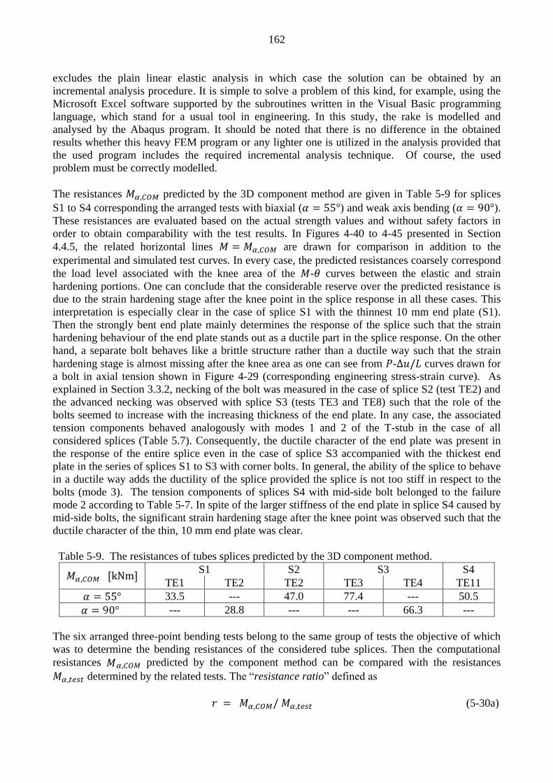
162

excludes the plain linear elastic analysis in which case the solution can be obtained by an

incremental analysis procedure. It is simple to solve a problem of this kind, for example, using the

Microsoft Excel software supported by the subroutines written in the Visual Basic programming

language, which stand for a usual tool in engineering. In this study, the rake is modelled and

analysed by the Abaqus program. It should be noted that there is no difference in the obtained

results whether this heavy FEM program or any lighter one is utilized in the analysis provided that

the used program includes the required incremental analysis technique. Of course, the used

problem must be correctly modelled.

The resistances predicted by the 3D component method are given in Table 5-9 for splices

S1 to S4 corresponding the arranged tests with biaxial ( ) and weak axis bending ( ).

These resistances are evaluated based on the actual strength values and without safety factors in

order to obtain comparability with the test results. In Figures 4-40 to 4-45 presented in Section

4.4.5, the related horizontal lines are drawn for comparison in addition to the

experimental and simulated test curves. In every case, the predicted resistances coarsely correspond

the load level associated with the knee area of the - curves between the elastic and strain

hardening portions. One can conclude that the considerable reserve over the predicted resistance is

due to the strain hardening stage after the knee point in the splice response in all these cases. This

interpretation is especially clear in the case of splice S1 with the thinnest 10 mm end plate (S1).

Then the strongly bent end plate mainly determines the response of the splice such that the strain

hardening behaviour of the end plate stands out as a ductile part in the splice response. On the other

hand, a separate bolt behaves like a brittle structure rather than a ductile way such that the strain

hardening stage is almost missing after the knee area as one can see from - curves drawn for

a bolt in axial tension shown in Figure 4-29 (corresponding engineering stress-strain curve). As

explained in Section 3.3.2, necking of the bolt was measured in the case of splice S2 (test TE2) and

the advanced necking was observed with splice S3 (tests TE3 and TE8) such that the role of the

bolts seemed to increase with the increasing thickness of the end plate. In any case, the associated

tension components behaved analogously with modes 1 and 2 of the T-stub in the case of all

considered splices (Table 5.7). Consequently, the ductile character of the end plate was present in

the response of the entire splice even in the case of splice S3 accompanied with the thickest end

plate in the series of splices S1 to S3 with corner bolts. In general, the ability of the splice to behave

in a ductile way adds the ductility of the splice provided the splice is not too stiff in respect to the

bolts (mode 3). The tension components of splices S4 with mid-side bolt belonged to the failure

mode 2 according to Table 5-7. In spite of the larger stiffness of the end plate in splice S4 caused by

mid-side bolts, the significant strain hardening stage after the knee point was observed such that the

ductile character of the thin, 10 mm end plate was clear.

Table 5-9. The resistances of tubes splices predicted by the 3D component method.

S1 S2 S3 S4

TE1 TE2 TE2 TE3 TE4 TE11

33.5 --- 47.0 77.4 --- 50.5

--- 28.8 --- --- 66.3 ---

The six arranged three-point bending tests belong to the same group of tests the objective of which

was to determine the bending resistances of the considered tube splices. Then the computational

resistances predicted by the component method can be compared with the resistances

determined by the related tests. The “resistance ratio” defined as

(5-30a)

163

describes the degrees of utilization of the splice only if the associated test is conducted. The splice

can have additional resistance in reserve after reaching the predicted resistance only if

. The largest value of the ratio was 0.78 whilst the smallest one was

0.67 as one can conclude by Tables (5-10) and (5-12). The average and standard deviation of are

0.74 and 0.037, respectively. It should be mentioned that the value of was obtained for the

average when it is calculated for the four conducted biaxial tests only, i.e., when the weak axis tests

are excluded. In any case, evidence based on the relative small number of the arranged tests show

that the enlargement of the 3D component method based on the simple rake is able to predict the

resistance of the splice with considerable reserve over the predicted value. This corresponds fully

the T-stubs ideology employed in design of the end plated splices in EC3: the end plate works in the

flanged connection as a part, which guarantees both the reserve in resistance and the sufficient

ductility of the connection including bolts as brittle part of the connection. The end plates fabricated

of unalloyed steel, is a largely used and successful example on a well functioning structural

solution. The above comparisons imply that the character of the ductile end plates is taken in the

account also in the solution by the 3D component method. Thus, there is no reason yet why the 3D

component method cannot be used for the design of tube splices. Next, the study on the 3D

component method is completed by enlarging the restricted validation data into to the case of

arbitrary biaxial bending through numerical analyses supported by the test results. The suggestion

then is: together with the physical reasoning and numerically expanded results, the validity of the

rake model defined in compliance with the component method can be shown to be reasonable at

least in the case of the resistance predictions.

Above, the flexural resistance was compared with the resistance obtained in the test.

If the test result is not available, Eq. (5-30a) can be replaced by

, (5-30b)

where represents the numerically enlarged data based on the FE analysis supported by the

test results. In Table 5-10, the ratio is presented for splices S1 to S3 in the cases of strong axis

( ), biaxial ( ) and weak axis ( ) bending such that those values, which are

based on the direct comparison with the tests, are shown as bold. The absolute reserve in resistance

can be expressed as

, (5-31)

when the is is the relative reserve. Because of the important role of the bent end plate as

part of the tension components – and, furthermore, in the response of the whole splice under

bending – the tension tests for the specimen made of the end plate material is used here as a

reference case. In order to do this, the relative reserve of the splice under bending is

compared with the relative reserve of the tension specimen through the ratio defined as

, (5-32)

where is given in Table (5-6) for splices S1 to S4. If the ratio disappears, the same relative

reserve in resistance would be expected from the splice under bending as from the tensile test

conducted for the end plate material. If it is negative, the relative reserve of the splice is smaller

than in the reference tension test; conversely, if it is positive, the relative reserve of the splice is

larger than observed in the tension case. The relative reserve ratios calculated according to Eq. (5-

32) are shown for splices S1 to S3 in Table 5-11, where the differences are given as

164

percentages of relative resistance observed in the tensile tests for the end plate material.

According to Table 5-11, the thickening end plate and decreasing weaken the relative

reserve ratio of the splice under bending. Only splice S1 under weak axis and biaxial bending has

larger relative reserve than measured for the related tensile test specimen, which is due to the

flexible behaviour of the thin end plate in bending. In all other cases, the relative reserve is smaller

than the related tensile test specimen has. As smallest, the relative reserve of the splice was

smaller than the relative reserve in the corresponding tensile test in the case of splice

S3 under strong axis bending. Then the role of the bolts is obviously larger than in any other case.

The relative reserve ratio of splice S2 with the medium end plates thickness seems to be somewhere

between the splices S1 and S3 with the thinnest and thickest end plates, respectively.

Table 5-10. Resistance ratios for splices S1 to S3.

* = Reference values for comparison.

Table 5-11. Relative resistance ratios for splices S1 to S3 in respect to the reference case.

In Table 5-12, the values of the resistance ratio are given for splice S4. The largest value of was

0.77 in the case of strong axis bending ( ), and all three values of were quite near each

other, such that the relative reserve in all directions deviated only slightly from the strength ratio

obtained in the tensile test for the related end plate. This is in line with the relatively small

values of ratio given to splice S4 in Table 5-13 (ranging between -3.5% and -12%), which imply

that this splice has coarsely the same relative reserve as the tensile test specimen. Splice S4 with

mid-side bolts behaves in somewhat less ductile way than splice S1 equipped with corner bolts

although their end plates have the same thickness ( ). The less ductile behaviour of S4

is in accordance with the failure mode 2 determined for its tension components (Table 5-7) whilst

tension components of splice S1 belong to mode 1.

Table 5-12. Resistance ratios for strong axis, biaxial and weak axis bending of S4.

or

S1

(method 2) S2 S3

Strong axis bending ( ) 0.76 0.81 0.88

Biaxial bending ( ) 0.73 (test) 0.75 (test) 0.78 (test)

Weak axis bending ( ) 0.67 (test) 0.76 0.74 (test)

0.74* 0.71* 0.67*

[%] S1

(method 2) S2 S3

Strong axis bending ( ) -7.7 -34 -63

Biaxial bending ( ) 3.8 -14 -33

Weak axis bending ( ) 27 -17 -21

or S4 (method 2)

Strong axis bending ( ) 0.77

Biaxial bending ( ) 0.75 (test)

Weak axis bending ( ) 0.76

(for comparison) 0.74

165

Table 5-13. Relative resistance ratios for splice S4 in respect to the reference case.

5.6.2 Moment-moment interaction curves

The bending resistances and are measured from the origin of the moment-moment

plane along the same line crossing the associated interaction curves in the failure points. The

distance between them represents the reserve over the resistance predicted by

the 3D component method. The character of the numerically enlarged failure curves was explained

in Section 4.5.2, where the - curves are shown in Figures 4-48 and 4-51 for splices S1 to S4

(continuous lines). For each splice S1 to S4, the failure curve (marked as - instead of - )

determined by the rake is presented and compared with the related, numerically enlarged failure

curve drawn in the same figure.

Since the rakes are defined for splices S1 to S4, their responses can be determined, in principle, for

the monotonically increased bending moment in the arbitrary direction after which the moment-

moment interaction curves called - curves can be drawn. These curves are defined in

compliance with Figure 5-3 such that and stand for, respectively, the strong and weak axis

bending components and of the resultant bending moment in the

direction of the angle . For simplicity, the subscripts referring to the resistance values are omitted

( and ). It should be noted that in the interaction curves drawn in the -

plane, the weak axis component and the strong axis component correspond to the

horizontal and vertical axis, respectively. In the moment-moment plane, the angle must be

measured clockwise from the vertical axis in order to be defined consistently with Figure 5-3.

Correspondingly, it holds that in strong axis bending ( ) and in weak

axis bending ( ). In the - plane, moreover, the resistance in the direction

, measured clockwise from the axis (vertical), represents the distance from the

origin to the failure point of the interaction curve. The - curves of Figures 5-16 and 5-19 are

drawn based on the discrete set of the calculated resistance values, which are solved for

monotonically increasing bending moment in cases , , , ,

, , , , , and . By connecting the failure

points with straight lines, the polygonal chain approximating the - curve in the first quarter of

the coordinate plane can be constructed. In addition, the interaction curve can be enlarged to the

other three quarters of the moment-moment plane such that the failure curve can be drawn for

. The “full circuit curves” are presented instead of the “first quarter curves” only for

obtaining a more illustrative appearance.

The failure curves predicted through the 3D component model (continuous lines) for splices S1 to

S3 are shown in Figures 5-16 to 5-19, respectively. For splices S1 and S4, the neglected curves

based on the method 1 (dotted line) are inside the relevant ones based on method 2. In addition to

the tests points, the numerically enlarged failure curves (dashed line) are shown in all figures. It

[%] S4 (method 2)

Strong axis bending ( ) -12

Biaxial bending ( ) -3.8

Weak axis bending ( ) -7.7

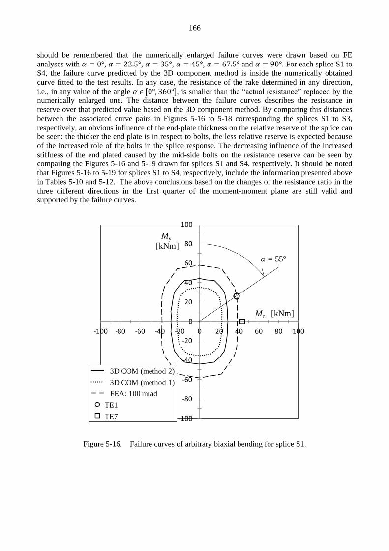
166

-100

-80

-60

-40

-20

0

20

40

60

80

100

-100 -80 -60 -40 -20 0 20 40 60 80 100

My

[kNm]

Mz [kNm]

3D COM (method 2)

3D COM (method 1)

FEA: 100 mrad

TE1

TE7

α = 55

should be remembered that the numerically enlarged failure curves were drawn based on FE

analyses with , , , , and . For each splice S1 to

S4, the failure curve predicted by the 3D component method is inside the numerically obtained

curve fitted to the test results. In any case, the resistance of the rake determined in any direction,

i.e., in any value of the angle , is smaller than the “actual resistance” replaced by the

numerically enlarged one. The distance between the failure curves describes the resistance in

reserve over that predicted value based on the 3D component method. By comparing this distances

between the associated curve pairs in Figures 5-16 to 5-18 corresponding the splices S1 to S3,

respectively, an obvious influence of the end-plate thickness on the relative reserve of the splice can

be seen: the thicker the end plate is in respect to bolts, the less relative reserve is expected because

of the increased role of the bolts in the splice response. The decreasing influence of the increased

stiffness of the end plated caused by the mid-side bolts on the resistance reserve can be seen by

comparing the Figures 5-16 and 5-19 drawn for splices S1 and S4, respectively. It should be noted

that Figures 5-16 to 5-19 for splices S1 to S4, respectively, include the information presented above

in Tables 5-10 and 5-12. The above conclusions based on the changes of the resistance ratio in the

three different directions in the first quarter of the moment-moment plane are still valid and

supported by the failure curves.

Figure 5-16. Failure curves of arbitrary biaxial bending for splice S1.

167

-100

-80

-60

-40

-20

0

20

40

60

80

100

-100 -80 -60 -40 -20 0 20 40 60 80 100

My

[kNm]

Mz [kNm]

3D COM

FEA: 40 mrad

T2

α = 55

-120

-100

-80

-60

-40

-20

0

20

40

60

80

100

120

-120 -100 -80 -60 -40 -20 0 20 40 60 80 100 120

Mx

[kN

m]

Mz [kNm]

3D COM

FEA: max

T3

T8

Figure 5-17. Failure curves of arbitrary biaxial bending for splice S2.

Figure 5-18. Failure curves of biaxial bending for splice S3.

168

-120

-100

-80

-60

-40

-20

0

20

40

60

80

100

120

-120 -100 -80 -60 -40 -20 0 20 40 60 80 100 120

My

[kNm]

Mz [kNm]

3D COM (method 1)

3D COM (method 2)

FEA: 50 mrad

TE11

Figure 5-19. Failure curve of biaxial bending for splice S4.

5.6.3 Validity of the resistance prediction by the rake model

The validity of the 3D component method of predicting the resistance of the tube splice is

investigated. The response of the considered splices depends decisively on the tension components

each of which is comprised of the end plate in bending and bolt(s) in tension. The active

compression components do not essentially deform because of their large stiffness in comparison

with the stiffness of the tension components. The tension components are modelled through the T-

stub analogy, which can be used generally whether the tube splice or any other type of joint with the

bolted end plate in tension is considered. In the failure modes of the tension component, which are

analogical with the failure modes 1 and 2 of the T-stub, the end plate deforms permanently such that

the ductile role of the end plate can be exploited. The predicted resistance of the tension

components can then be associated with the load level reached in the knee area between the elastic

and the strain hardening stages of the response. Then the reserve in resistance is directly due to the

strain hardening stage after the knee area such that this reserve depends decisively on the ductility

of the bent end plate. When the validity of the 3D component method is studied, the key question is:

does the reserve in resistance predicted for the separate tension component guarantee the validity of

the 3D component model, i.e., the validity of the rake.

In Section 5.6.1 and 5.6.2, the (biaxial) bending resistances of the considered tube splice, which

were predicted by the 3D component method, were compared with the test results and with the

numerically enlarged resistances. Based on the comparison with the resistances attained in the six

169

arranged tests, the average value of the resistance ratio was 0.74 indicating clear reserve over the

predicted resistances. In addition, the comparisons with the numerically enlarged resistances

showed that:

1. The resistance predicted by the rake was in the knee area of the experimental (and

simulated) moment-rotation curve of the splice in all cases (Figures 4-40 to 4-45).

2. The resistance ratio satisfies the requirement for tube splices S1 to S4 under biaxial

bending in the arbitrary direction (Figures 5-16 to 5-19).

3. The relative reserve depends as expectedly on the mutual relation between the roles of

the end plate (ductile) and bolt (less ductile) in the splice response.

The latter was revealed by comparing the splice resistance obtained by the 3D component method

with the experimental and numerically enlarged resistances in the cases of weak axis, biaxial and

strong axis bending (Tables 5-10 to 5-13). The three items presented above describe the physical

character of the splices such that these support the validation of the 3D component method based

directly on the comparison with the quite restricted number of tests. In the prevailing standard, the

component method is intended mainly for the problems with joints under strong axis bending. For

considered splices, the largest resistance ratio, i.e., the lowest relative reserve, was obtained in the

strong axis bending according to Tables 5-10 to 5-13. Then one can suggest that the 3D component

method for the arbitrary biaxial bending should be approved in the condition that it is acceptable in

the strong axis bending case (as it is).

Altogether, the 3D component method embedded in a simple rake model can be judged as

validated when predicting the resistances of the tube splices. It should be emphasized that in all

considered splices, the end plates had sufficient flexibility in respect to the bolts, such that either

mode 1 or mode 2 failure was determinate. No splices obeying failure mode 3 (bolt failure) were

considered. This would also be unnecessary because it is immaterial whether failure mode 3 is

related to the 2D or the 3D solution because the brittle character of the bolts prevails in both cases.

The use of bolted end plates, the failure of which represents mode 3, is not advisable in the tension

zone because of the decisive role of the bolts.

5.6.4 Remarks on ductility and FE simulations

In the rake model, the elastic-ideally plastic deformability curves were adopted to the components.

The initial stiffness is obtained as a function of the initial stiffnesses of the active components in the

rake. However, the stiffness of the rake can be accurate only when it is based on the accurate

component stiffnesses, which were missing and replaced by the approximate values. With the

increasing load, the components reach their plastic strengths one at a time. An abrupt decrease in

the slope always occurs when the next component starts to yield and the global response can be

prescribed as the sequence of the straight lines. For those components, which have reached their

resistances, the sufficient ability to yield is assumed, i.e., these components must be ductile such

that the resistance of the rake can be obtained. When the rake yields, its global response is

horizontal. The adequacy of rotation capacity (ductility) of a joint with a bolted end plate can be

evaluated according to EC3 (Section 6.4.2) for the purposes of plastic global analysis (of frames).

The ductility of the individual components is not discussed in the standard.

170

The adequate rotation capacity is obtained according to the standard when the thickness of the end

plate (in the splice) is less than a given limit value, or , where is the diameter

of the bolt and and are, respectively, the bolt strength and yield strength of the end plate

(6.4.2 (2) in EN 1993-1-8). When evaluated by the nominal values of the splices, the limit thickness

of . Thus, only those of the considered splices that are

equipped with the thinnest, 10 mm end plates satisfy this condition. The series of bending tests

representing the splices with the four-bolt layout and the corner bolts (S1 to S3) is considered,

based on the observed maximum rotations given in Table 3-10 and 3-11. As expected, the

maximum rotations of the splices with 10 end plates were large (117 mrad and 152 mrad in tests

TE1 and TE7, respectively). However, the maximum rotation of the splice with the 15 mm end

plate was also large (96 mrad in test TE2), and even the smallest obtained maximum rotations for

the splice with the thickest, 20 mm end plate implied significant ability to undergo rotations (50

mrad and 67 mrad in tests TE3 and TE8, respectively). In fact, the limit thickness for the plastic

frame analysis given in the standard may be too severe in the case of the corner bolts due to the

flexible response of the extended end plates with the corner bolts. Consequently, to fully utilise the

resistances intended for the associated corner components, the limit thickness of the end plate for

the plastic design of frames may need to be increased. For the tension components in the splice with

the four-bolt layout and the mid-side bolts, the limit thickness given in the prevailing standard may

be, conversely, too large due to its larger stiffness. Before the suggested tension components can be

employed in the design, questions related to the ductility and rotation capacity should be

investigated properly.

FE analyses of the tension components. The structural model for the elastic-plastic, 3D FE

simulations of the splice is axial tension was introduced in Section 4.2.4. The behaviour of splice S1

in axial tension was simulated as an example in Appendix A4, such that the main interest was in the

roles of prying action and contacts between the end plates. Splice S1 in axial tension was also

introduced as a “third elementary problem” for the convergence tests in Section 4.3. In Appendix

A5, the properties of the tension components were compared with the responses predicted by the FE

analysis of the splices S1 to S4 in axial tension. There was no direct validation data for the

numerical model of the splices under axial tension. However, the same tension components that are

active in the splice in axial tension are active and play the decisive role in the rotational behaviour

in the splice under bending. In this mind, the validity of the FE models of splices in axial tension

was indirectly studied when the simulations of the bending tests were compared with the test

results. The use of numerical models as a tool in the development of the components is

demonstrated by the examples and, in addition, the influence of the selected factors, including the

effect of weld size, on the splice behaviour was investigated through the numerical simulations. In

Appendix A5, the roughly approximated (tentative) stiffness values are compared with those

estimated by 3D FE simulations on splices in axial tension. A procedure by which the stiffnesses

are fitted to the numerically computed values is described. It is emphasized that without the

properly validated model, the suggested procedure has only demonstrative significance. These

considerations are placed in the appendix because they can be seen as complementary in relation to

the main objectives of the thesis.

171

6 CONCLUSIONS

The motivation of this study is to develop the design method suitable for the three-

dimensional modelling and analysis of structural steel joints. The practical research tasks

were defined through the end-plated splices of the rectangular tube. The main objective was to

show that the 3D component model can predict the resistance of the tube splice under biaxial

bending. Four different splices (S1 to S4) were introduced as the driving examples of the

study. These splices were selected such that the focus will be in the behaviour of the tension

components, which were modelled exploiting the T-stub analogy. The responses of these

splices were experimentally investigated through six tests including biaxial and weak axis

bending tests, which were simulated by the 3D FE method. The validity of the numerical

models was studied against the test results such that these models could be further utilized as

the research tool. The suggested 3D design model of the splice was based on a simple

mechanical system called a rake, which was defined in compliance with the principles of the

component method. The validity of the rake model was judged through the comparisons

between the predicted resistances and the validation data, which was based on resistances

directly obtained by the tests and the numerically enlarged data supported by the tests. The

conclusion based on the small amount of the tests was completed by the physical reasoning.

The results and conclusions of the thesis have already been discussed in the associated

sections in detail. Next, these conclusions are presented like a summary account.

6.1 Empirical study

The bending tests were arranged in order to cast experimental foundation for the used

computational models whether they were based on the component method or the advanced

numerical analysis. Any reports on the separate joint tests for biaxial bending were not found

in the literature. The inventive testing arrangements and the test results were described. The

force of the jack was controlled in the loading procedure the main objective of which was to

determine the resistance of the specimen. In the biaxial tests, the inclination of the initially

vertical jack was inevitable due to the transverse displacement because of asymmetric

bending. However, the inclination remained small enough in each test arranged such that the

approximation on vertical loading was still valid. Then the test results were simple to interpret

in spite of the small inclination of the jack. It is emphasized that this test type, which was

successful with the considered tube splices, may fail with the other type of the specimens,

especially, when the ratio between weak and strong axis bending stiffness of the tube or its

splice is small or because of weak torsional stiffness (open profiles). In any case, the focus of

the thesis was in the flexural resistance dependent decisively on the deformations in the

tension zone of the splice.

The main factors varied in the tests were the direction of the resultant bending moment, end

plate thickness and layout of the splices. The bolts with the same size and grade were used in

all tests. The test series for three splices with the same layout but the varied thickness showed

that the end plate thickness is the decisive factor affecting the stiffness, the failure mode and

the resistance of the splice. The layout with the corner bolts represented the weakest possible

placing of the bolts in that mind explained in Section 2.2.6. The splice equipped with the mid-

side bolt showed the essentially larger stiffness and resistance than the corresponding splice

with the corner bolts. All tests arranged under the control of the jack force were terminated

when the (global) response was (almost) horizontal mainly because of the plastic

deformations. No bolt failure occurred in any tests in spite of the advanced necking of the bolt

172

shank in some tests. The opened cracks were observed in those tests arranged with the

thinnest end plate but not until the end of the tests. It is emphasized that the analogy between

the observed failure modes and those related to the plastic failure modes of the T-stub

introduced in EC3 could be identified in the tests (in the tension zone of the splices). Thus,

the exploitation of the plasticity theory including yield line mechanism seems to be

reasonable in the analysis of the end plates as embedded in the component method.

6.2 Numerical study

The numerical analyses of the considered splices were accomplished as the elastic-plastic

simulations by the three-dimensional finite element (3D FE) method. The structural models

used in the analyses of the splices were introduced and the correspondence between the model

and the loading arrangement was discussed. The small inclination angle of the jack load in the

tests is the prerequisite for the justified use of the simplified model with the vertical load. The

description of the plastic behaviour including the strain hardening stage was based on the

classical plasticity theory (von Mises). The uniaxial stress-strain curves were constructed

according to that data given in the steel certificates and then it was generalised into a 3D

constitutive law supported by the results of the SINTAP project. The yielding without the

sharply defined yield point was described by the formulas adopted from the Ramberg-Osgood

model (for bolts and tubes). The sharp yield point was presented through the model including

the elastic phase, yield plateau and strain hardening stage the latter of which was defined as a

power law type of formula (for end plates). The significant hardening behaviour typical for

the non-alloyed steels used in the end plates can then be taken into account in a reasonable

way. Material fracture and its consequences cannot be described by the elastic-plastic model.

Contacts present at the splice were modelled as a simplified way such that (normal) contacts

between the end plates can change, i.e., the contact force and area can vary during the loading,

whilst other contacts in the connections are assumed to remain as constant.

The bending tests on tube splices were numerically simulated and the computed results were

compared with the test results. The elastic-plastic response of a splice to monotonically

increasing bending moment (in the fixed direction) was followed beyond the limit point,

which stands for the theoretical maximum load before the softening stage. The converged

solutions were obtained through the incremental and iterative procedure under the

displacement control employed through enforced vertical displacement. The premature failure

due to cracking cannot be predicted by the elastic-plastic simulation. Thus, the elastic-plastic

model predicts the resistance accurately only when plastic behaviour is decisive up to the

(theoretical) limit point. This occurred in the tests with the thickest end plate (splice S3) when

necking occurring in the tension bolt(s) determines the resistance of the splice. Oppositely,

the large bending deformations in the strongly bent, thin end plates (splices S1, S4) caused

cracking in the tests, which is not taken into account by the computational model. On the

other hand, the initial stiffness of the splice was predicted quite well for splices with the

thinnest end plates and less accurately with the thicker end plates. The poorest stiffness

prediction was obtained in the case of the splice (S3) with the thickest end plate. The

consistent results on the comparison between the computed response and tests have been

reported in the literature when the corresponding elastic-plastic models have been utilised in

the analysis of the end plated connections as explained in Section 4. Obviously, poor

predictions of the initial stiffness were caused by the deficient description of the initial

imperfections, which affects the splice response more significantly in the case of thick end

plates. The initial imperfections are mainly due to the fabrication of the splice. The most usual

reason for them is the welding between the tube and end plate. In any case, despite its obvious

173

limitations related to the description of the initial imperfections and material fracture, the

elastic-plastic 3D FE analysis could be exploited as a useful research tool in this study.

Based on the elastic-plastic analyses, the theoretical bending resistance of the splice in the

arbitrary direction can be presented, for example, through the - interaction curve

expressed by the weak and strong axis components related to each plastic limit point. The

elastic-plastic failure curve does not take into account the premature failure of the splice

observed in some tests. Thus, a simple post-processing procedure was suggested through

which the FE analysis results were calibrated against to the resistances obtained in the

arranged tests. As a result, the resistances of each splice under arbitrary biaxial bending were

attained as a failure curve supported by the tests. A failure curve of this kind represents the

numerically enlarged validation data for the 3D component method. In spite of the obvious

limitations of the used elastic-plastic model, which allows limitless yielding, was employed as

the research tool when the resistances of the splices under arbitrary (biaxial) bending were

determined.

Theoretically interesting FE elastic-plastic simulation on the response of splice S1 in axial

tension is presented in Appendices A4. It should be emphasized that initial imperfections had

a minor influence on the splice response of splice S1 with flexible end plate (in respect to

bolts). The simulated response to axial normal force demonstrate the development of contacts

between the end plates during the loading and revealed, for example, that decreasing prying

action may sustain the stable response of the splice against the increasing axial load despite

the onset of necking in the tension bolt. This “decreasing prying” may occur also in the

tension zone of the splice under bending. In Appendix A5, the behaviour of the individual

tension component was simulated and the influences of the weld thickness and pre-tensioning

of the bolts on the response of the tension components are studied. Simulations on the splice

under biaxial bending are presented in Appendix A6.

6.3 3D component method

The study on the 3D component method was accomplished through the driving examples

chosen in order to find an answer to the research question (ii) set in Section 1.3. The objective

then was to formulate the 3D component method in compliance with the principles of the

(2D) component method introduced in the prevailing standard EN1993-1-8. The responses of

the considered splices under biaxial bending were analysed through the 3D model called a

rake. The resistances obtained by the 3D component method were compared with the

resistances determined by the tests and by the numerical analyses supported by the tests. It

should be emphasized that the stiffnesses used in the 3D component model, i.e., in the rake

model, were the approximate ones utilized only in order to determine the resistances by the

rake model.

The enlargement of the component method into 3D analysis is based on a simplified three-

dimensional mechanical model (one-layer rake) by which the analyses of the splices under

arbitrary biaxial bending could be performed. The relevant components of the splices were

identified first in the decomposition. The compression components are described as almost

incompressible and their strength is assumed to be sufficient. Then the main attention was in

the tension components. In the case of the symmetrically placed corner bolts in the end plates

(splices S1 to S3), the associated components were called corner components. The yield

mechanisms analogous with the T-stub were introduced to the corner components in order to

determine their resistances and failure modes. The tension component for the splice with the

174

mid-side bolts (splice S4) also was suggested based on the modified formulations of EC3

given to the extended end plate flange in the tension zone. The rake was assembled in order to

perform the 3D component analysis for splice under biaxial bending. Because of the tentative

character of the used stiffnesses of the tension components, the initial stiffness of the splice

represents a rough approximation. However, no attempt to derive the new stiffness formulas

was made in this thesis. Instead, an approach to the associated fitting problem was

demonstrated in Appendix A5, where the starting point for the stiffness formulation was taken

from prevailing standard. Anyway, there was no intention to investigate and develop the

stiffness formulations of EC3 in this thesis. The stiffness modelling and analysis will be an

obvious issue of further research. In addition, the ductility model for individual components

requires an attention when the component method is further developed.

In this thesis, the principal research task was to investigate the suitability of the rake model in

the resistance prediction of the splice under biaxial bending in the arbitrary direction. In order

to show the validity of the 3D component method, the bending resistances predicted by the

rake model was compared with the resistances obtained by the tests and by the numerical

means supported by the tests. Every considered splice had a substantial reserve in resistance

in respect to that predicted by the 3D component method, i.e., by the rake model. This reserve

was mainly due to the strain hardening of the end plate (in bending) being active in the

deformation of the end plated connection such that either the failure mode 1 or 2 of EC3 was

decisive. The relative reserve decreased because of the thickening (stiffening) of the end

plates, which was related to the increasing role of the bolts (in tension) as a deformable part of

the joint. Consistently, the resistance of the splice depended expectedly on the mutual roles of

the end plate and bolt(s) in the studied end plated connection. Altogether, the comparisons

between the predicted resistances and the validation data gave understandable results on the

light of physical reasoning, which substantiate the evidence for the validity of the 3D

component method. Thus, the 3D component method embedded in a simple rake model can

be judged to be as validated in respect to the resistance prediction in the case of the studied

tube splices under biaxial bending. Moreover, the smallest relative reserves were obtained in

the case of strong axis bending in each splice. Based on this observation, one can suggest that

the resistance predicted by the 3D component method for the arbitrary biaxial bending can be

approved provided that the predicted resistance in strong axis bending is acceptable. It is

emphasized that the strong axis bending case represents the solution by the prevailing

component method introduced in 2D.

6.4 Final remark

Because of the generic character of the component method, this method is suitable not only

for the analysis of the tube splices under biaxial bending but also for the analysis of many

other types of joints under the different 3D loading conditions. If the component method will

be enlarged, the validity of the method should always be based on sufficient experimental

evidence. Without the tests, the (2D or 3D) component method is based only on the

engineering intuition. Thus, the enlargement of the component method into 3D analysis tool

for the structural design will probably be a possible but very laborious procedure requiring

large experimental program. The numerical methods as supported by the tests would also play

an important role then. The modelling of the initial imperfections and material fracture are the

issues, which deserve attention when the numerical models of the end plated connections are

studied in future.

REFERENCES

NOTE: Standards are placed at the bottom

Abaqus manual (2010), Abaqus 10.6 documentation, Available also as on-line manual loaded with

the associated program version. Parts especially referred to are

Abaqus Analysis User’s Manual

Abaqus Theory Manual

Agerskov H. (1976), High-strength bolted connections subject to prying, Journal of the structural

division, ASCE, vol. 102, No. ST2, pp. 161-175.

Agerskov H. (1988), Bolted end-plate connections in steel structures, Connections in steel

structures, Proceedings of a state of art workshop on connections and the behaviour, strength and

design in steel structures (held in May 25-27 1987 in France), pp. 52-59.

Airila M, Ekman K., Hautala P (2003), Koneenosien suunnittelu (in Finnish), WSOY, Suomi.

Atlas of stress-strain curves (2002), 2nd

edition, ed. by Y. Tamarin, ASM International.

Babuska I., Oden T. (2003), V&V in computational engineering and Science, Part I: Basic

concepts. Institute for Computational Engineering and Sciences (ICES), University of Texas at

Austin, USA.

Bathe K.-J., Bouzinov, P. A. (1997), On the constraint function method for contact problems,

Computers and Structures, vol. 64, pp. 1069-1085.

Bathe K.-J., Ramm E., Wilson E. L. (1975), Finite element formulations for large deformation

dynamic analysis, International Journal for Numerical Methods in Engineering, vol. 9, pp. 353-

386.

Bjorhovde R., Brozetti J., Colson A. (1990), Classification system for beam-to-column connections,

Journal of Structural Engineering, ASCE, vol. 116, pp. 3059-3076.

Bannister A. C, Trail .S. J.. (1996), Structural integrity assessment procedures for European

industry, SINTAP, Contribution to sub-task 2.1: The significance of yield stress/tensile stress ratio

to structural integrity. British Steel plc, Swinden technology Centre, UK.

Bannister A. C. (1998), Structural integrity assessment procedures for European industry, SINTAP,

Contribution to sub-task 2.3: Assessment of the occurrence and significance of yield plateaus in

structural steels. British Steel plc, Swinden technology Centre, UK.

Bannister A. C., Ruiz Ocejo J., Guttierrez-Solana F. (2000), Implications of yield stress/tensile

stress ratio to the SINTAP failure diagrams for homogeneous materials, Engineering Fracture

Mechanics, vol. 67, pp.547-562.

Bower A. F. (2012), “Applied mechanics of solids” in the internet page named solimechanics.org.

Published also as printed copy by CRC press (2010), USA.

Bursi O. S., Jaspart J.-P. (1997a), Benchmarks for finite element modelling of bolted steel

connections, Journal of Constructional Steel Research, vol. 43, nos 1-3, pp. 17-42.

Bursi O. S., Jaspart J..-P. (1997b), Calibration of finite element model for isolated bolted end-plate

steel connections, Journal of Constructional Steel Research, vol. 44, No. 3, pp. 225-262.

Bursi O. S., Jaspart J. -P. (1998), Basic issues in the finite element simulation of extended end plate

connections, Computers & Structures, vol. 69, pp. 361-362.

Celikag M., Kirby P. A. (1989), Out-of-plane moment rotation response for common joints. in

International Colloquium, Bolted and special structural connectors, held in May 15-20, 1989 in

USSR, Moscow, pp. 136-142.

Celikag M., Kirby P. A. (1987), Standardised method for measuring 3-dimensional response of

semi-rigid joints, in Connections in steel structures, in Proceedings of a state of art workshop on

connections and the behaviour, strength and design in steel structures, held in May 25-27 1987 in

France, pp. 203-210.

Chakrabarty J. (2006), Theory of Plasticity (3rd

edition), Elsevier Butterworth-Heinemann.

Chen W. F., Han D. J. (1988), Plasticity for Structural Engineers, Springer-Verlag, Printed in USA.

Cook R. D., Malkus D. S., Plesha M. E. (1989), Concepts and applications of finite element

analysis, Third edition, John Wiley & Sons, Inc, Printed in Singapore.

Cook R. D., Malkus D. S., Plesha M. E., Witt R. J. (2002), Concepts and applications of finite

element analysis, Forth edition, John Wiley & Sons, Inc, USA.

Crisfield M. A. (1991), Non-linear finite element analysis of solids and structures, Volume 1, John

Wiley & Sons Ltd., England.

Diaz C., Victoria M., Mart P., Querein O. M. (2011), FE model of beam-to-column extended end-

plate joints, Journal of Constructional Steel Research, vol. 67, pp. 1578-1590.

Feldmann M., Sedlacek G., Weynand K. (1996), Safety considerations of Annex J of Eurocode 3, in

Connections in steel structures III, behaviour, strength & design (edited by Reidar Bjorhovde),

Elsevier Science, U.K.

Fung Y. C. (1994), A first course in continuum mechanics, Third edition, Prentice-Hall, USA.

Gir o Coelho A. (2004), Characterization of the ductility of bolted end plate beam-to-column steel

connections, PhD dissertation, University of Coimbra, Portugal.

Gir o Coelho A. M., Biljaard F.S.K., Gresnigt N., Sim es da Silva L. (2004), Experimental

assessment of the behaviour of bolted T-stub connections made up welded plates, Journal of

Constructional Steel Research, vol. 60, pp. 269-311.

Gresnigt A.M., Romeijn A., Wald F., Steenhuis C.M. (2008), Column bases in shear and normal

force, Heron, vol. 54, issue 1/2 (Special issue: Steel column bases), pp. 87-108.

Heinisuo M., Laine V., Lehtimäki E. (2009), Enlargement of the component method into 3D,

Proceedings: Nordic Steel Constructional Conference 2009, Malmö, Sweden, pp. 430-437.

Heinisuo M., Ronni H., Perttola H., Aalto A., Tiainen T. (2012a), End and base plate joints with

corner bolts for rectangular tubular member, Journal of Constructional Steel Research, vol. 75, pp.

85-92.

Heinisuo M., Perttola H., Ronni H. (2012b), Component method for end plate joints, modeling of

3D frames: literature review, Steel Construction, Design and Research, Vol. 5, No. 2, pp. 101-107.

Heinisuo M., Perttola H., Ronni H. (2014), A step towards the 3D component method for modelling

beam-to-column joints, Steel Construction, Vol. 7, No. 1, pp. 8-13.

Jaspart J.-P. (1991), Etude de la semi-rigidit des noeuds poutre-colonne et son influence sur la

r sistance et la stabilite des ossatures en acier, PhD dissertation, University of Li ge, Belgium

Jaspart J.-P. & Vandegans D. (1998), Application of the component method to column bases,

Journal of Constructional Steel Research, vol. 48, pp. 89-106.

Jaspart J.-P. (2000), General report: session on connections, Journal of Constructional Steel

Research, vol. 55, pp. 69-89.

Jaspart J.-P. Wald F., Weynand K., Gresnigt A.M. (2008), Steel column base classification, Heron,

Vol. 54, issue 1/2 (Special issue: Steel column bases), pp. 69-86.

Kikuchi N., Oden T. J. (1988), Contact problems in elasticity: A study of variational Inequalities

and finite element methods, Siam, Philadelphia, USA.

Kloosterman G. (2002), Contact methods in finite element simulations, Ponsen&Looijen,

Wageningen, Nederland.

Konter A. (2000), How to – undertake a contact and friction analysis, NAFEMS Ltd, Glasgow,

Scotland.

Laine V. (2007), Development of semi-rigid behaviour of structural connections in an integrated

design system, Master of Science Thesis (written in finnish), Tampere University of Technology,

Mechanical Engineering, Finland, 104 p + app. 20 p.

Lee D-Y., Goel S., Stojadinovich B. (2008), Exposed Column-Base Plate Connections Bending

About Weak Axis: II. Experimental Study, Steel Structures, vol. 8, pp. 29-42.

Ling Y. (1996), Uniaxial true stress–strain after necking. AMP Journal of Technology, vol. 5, June,

pp.37-48.

Lubliner J. (1990), Plasticity theory, Macmillan publishing company, New York.

Malvern L. E. (1969), Introduction to the mechanics of a continuous medium, Prentice-Hall, USA.

Mattiasson K. (1981), Continuum mechanics principles for large deformation problems in solid and

structural analysis, Publication 81:6, Chalmers University of Technology, Göteburg, Sweden.

Mirambell E., Real E. (2011), On the calculation of deflections in structural stainless steel beams:

an experimental and numerical investigation, Journal of Constructional Steel Research, vol. 54,

pp.109-133.

Mäkinen J., Fränti K., Korhonen M., Fillion J., Heinisuo M. (2016), End-plate Connections in

Biaxial Bending – Measurements, 13th International Aluminium Conference, Sustainability,

Durability and Structural Advances, INALCO 2016, Naples, Italy, pp. 21-23.

Nethercot D., Zandonini R. (1989), Methods of prediction of joint behaviour: beam-to-column

connections. In Structural Connections -- Stability and Strength, ed. Narayanan R., Elsevier

Applied Science, England, pp. 23-62.

Perttola H., Heinisuo M. (2011), Test report, end plate joints of steel tubes, biaxial and weak axis

bending, Research Report 155, Tampere University of technology, Department of civil engineering,

Finland.

Perttola H., Heinisuo M. (2012), Experimental study of flanged joints of tubular members under

axial bending, in CONNECTIONS VII, 7th international workshop on connections in steel

structures, Timisoara.

Rasmussen K. J. R. (2001), Full-range stress-strain curves for stainless steel alloys, Research

Report No. R811, November 2001, The University of Sidney, Department of Civil Engineering,

Australia.

Rasmussen K. J. R. (2003,b), Full-range stress-strain curves for stainless steel alloys, Journal of

Constructional Steel Research, vol. 59, pp.47-61.

Rasmussen K. J. R. (2003,b), Reply to: Discussion of full-range stress-strain curves for stainless

steel alloys, Journal of Constructional Steel Research, vol. 59, pp.1325-1326.

Real E., Mirambel E., (2003), Discussion of full-range stress-strain curves for stainless steel alloys,

Journal of Constructional Steel Research, vol. 59, pp.1321-1323.

Ronni H., Heinisuo M. (2008), Test report, end plate joints of steel tubes, strong axis bending,

Research Report 149, Tampere University of technology, Department of civil engineering, Finland.

Ronni H., Heinisuo M. (2012), Test report, end plate joints of steel tubes, biaxial bending in fire,

Research Report 156, Tampere University of technology, Department of civil engineering, Finland.

Roylance D. (1996), Mechanic of Materials, John Wiley&Sons, New York.

Ruiz Ocejo J., Gutierrez-Solana F. (1998), On the strain hardening exponent definition and its

influence within SINTAP, Report/SINTAP/UC/07, University of Cantabria, Spain.

Schardt R. (1989), Verallgemeinerte technische Biegetheoty, Springer Verlag, Berlin.

Selamet S., Garlock M. (2010), Guidelines for modeling three dimensional structural connection

models using finite element methods, in Proceedings of the steel structures, Culture and

Sustainability (ECCS) Conference, Istanbul, Turkey.

Sim es da Silva L., Gir o Coelho A., Lucena Neto E. (2000), Equivalent post-buckling models for

the flexurala behaviour of steel connections, Computers and Structures, vol. 77, pp. 615-624.

Sim es da Silva L., Gir o Coelho A. (2001a), A ductility model for steel connections, Journal of

constructional steel research, vol. 57, pp. 45-70.

Sim es da Silva L., Gir o Coelho A. (2001b), An analytical evaluation of the response of steel

joints under bending and axial force, Computers and Structures, vol. 79, pp. 873-881.

Sim es da Silva L., Santiago A., Vila Real P. (2002), Post-limit stiffness and ductility of end-plate

beam-to-column steel joints, Computers and Structures, vol. 80, pp. 515-531.

Sim es da Silva L. (2008), Towards a consistent design approach for steel joints under generalized

loading, Journal of constructional steel research, vol. 64, pp. 1059-1075.

Sinclair G. B., Beisheim J. R., Sezer S. (2006), Practical convergence-divergence checks for

stresses from FEA, in Proceedings 2006 ANSYS users conference and exposition, 2-4 May 2006,

Pittsburgh, PA, USA.

Steenhuis C.M., Wald F., Sokol Z., Stark J.W.B. (2008), Concrete in compression and base plate in

bending, Heron, vol. 54, issue 1/2 (Special issue: Steel column bases), pp. 51-68

Steurer A. (1996), Trag- und Verformungsverhalten von auf Zug Beanspruchten Schrauben, Institut

für Baustatik und Konstruction, Eidgenössische Technische Hochshule (ETH) Zürich.

Szilard R. (1974), Theories and applications of plate analysis, classical, numerical and engineering

methods, Englewood Cliffs, NJ, Prentice-Hall.

Van der Vegte G. J., Makino Y. (2004), Numerical simulations of bolted connections: the implicit

versus the explicit approach, in Connections in steel structures V - June 3-4, 2004, Amsterdam,

Netherlands.

Wald F., Bouguin V., Sokol Z., Muzeau J-P. (2000), Effective length of T-stub of RHS column

base plates, in Proceedings of the Conference Connections in Steel Structures IV, Roanoke, pp. 393-

402.

Wald F., Sokol Z., Jaspart J.-P. (2008), Base plate in bending and anchor bolts in tension, Heron,

vol. 54, issue 1/2 (Special issue: Steel column bases), pp. 21-50.

Wald F., Sokol Z., Steenhuis C.M., Jaspart J. P. (2008), Component method for steel column bases,

Heron, vol. 54, issue 1/2 (Special issue: Steel column bases), pp. 3-20.

Wang W., Zhang, K. D. (1987), Elastic plastic behaviour investigation of externally, axially cracked

cylinder, International Journal of Fracture 34: R49-R52.

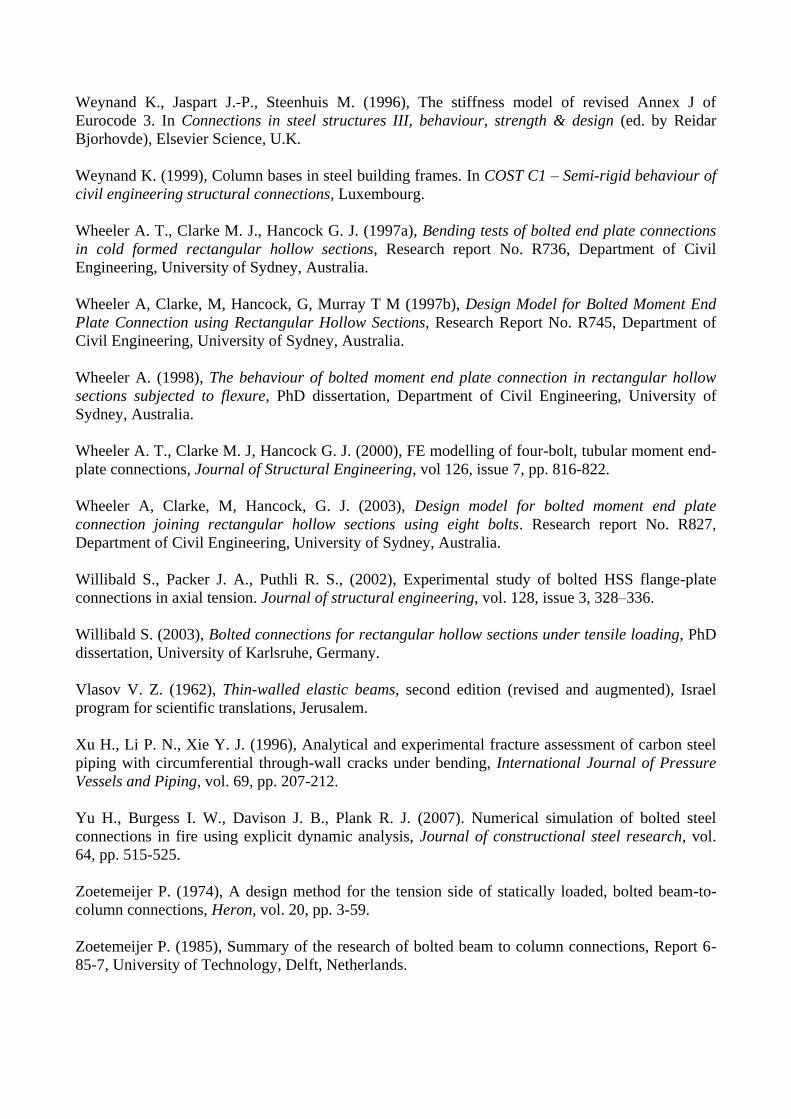
Weynand K., Jaspart J.-P., Steenhuis M. (1996), The stiffness model of revised Annex J of

Eurocode 3. In Connections in steel structures III, behaviour, strength & design (ed. by Reidar

Bjorhovde), Elsevier Science, U.K.

Weynand K. (1999), Column bases in steel building frames. In COST C1 – Semi-rigid behaviour of

civil engineering structural connections, Luxembourg.

Wheeler A. T., Clarke M. J., Hancock G. J. (1997a), Bending tests of bolted end plate connections

in cold formed rectangular hollow sections, Research report No. R736, Department of Civil

Engineering, University of Sydney, Australia.

Wheeler A, Clarke, M, Hancock, G, Murray T M (1997b), Design Model for Bolted Moment End

Plate Connection using Rectangular Hollow Sections, Research Report No. R745, Department of

Civil Engineering, University of Sydney, Australia.

Wheeler A. (1998), The behaviour of bolted moment end plate connection in rectangular hollow

sections subjected to flexure, PhD dissertation, Department of Civil Engineering, University of

Sydney, Australia.

Wheeler A. T., Clarke M. J, Hancock G. J. (2000), FE modelling of four-bolt, tubular moment end-

plate connections, Journal of Structural Engineering, vol 126, issue 7, pp. 816-822.

Wheeler A, Clarke, M, Hancock, G. J. (2003), Design model for bolted moment end plate

connection joining rectangular hollow sections using eight bolts. Research report No. R827,

Department of Civil Engineering, University of Sydney, Australia.

Willibald S., Packer J. A., Puthli R. S., (2002), Experimental study of bolted HSS flange-plate

connections in axial tension. Journal of structural engineering, vol. 128, issue 3, 328–336.

Willibald S. (2003), Bolted connections for rectangular hollow sections under tensile loading, PhD

dissertation, University of Karlsruhe, Germany.

Vlasov V. Z. (1962), Thin-walled elastic beams, second edition (revised and augmented), Israel

program for scientific translations, Jerusalem.

Xu H., Li P. N., Xie Y. J. (1996), Analytical and experimental fracture assessment of carbon steel

piping with circumferential through-wall cracks under bending, International Journal of Pressure

Vessels and Piping, vol. 69, pp. 207-212.

Yu H., Burgess I. W., Davison J. B., Plank R. J. (2007). Numerical simulation of bolted steel

connections in fire using explicit dynamic analysis, Journal of constructional steel research, vol.

64, pp. 515-525.

Zoetemeijer P. (1974), A design method for the tension side of statically loaded, bolted beam-to-

column connections, Heron, vol. 20, pp. 3-59.

Zoetemeijer P. (1985), Summary of the research of bolted beam to column connections, Report 6-

85-7, University of Technology, Delft, Netherlands.

Standards:

ASME V&V 10-2006 (2006), Guide for verification and validation in computational solid

mechanics, American Society of Mechanical Engineers, New York.

EN 10025-2 (2004), Hot rolled products of structural steels, Part 2: Technical delivery conditions

for non-allow structural steels, CEN, Brussels.

EN 10204 (2004), Metallic products: Types of inspection documents, CEN, Brussels.

EN 10219-1 (2006), Cold formed structural hollow sections of non-alloy and fine grain steels, Part

1: Technical delivery conditions, CEN, Brussels.

EN 1993-1-8 (2005), Eurocode 3: Design of steel structures, Part 1-8: Deign of joints, CEN,

Brussels.

ENV 1993-1-1 (1994), Eurocode 3: Revised Annex J, Design of steel structures, CEN, Brussels.

1

APPENDIX A1

3D PLASTICITY MODEL

A1.1 Classical metal plasticity ............................................................................................. 1

A1.2 Stable material based on work hardening .................................................................... 1

A1.3 Construction of the 3D constitutive models ................................................................ 3

The material models used in the elastic-plastic three-dimensional finite element analysis (3D

FEA) of the rectangular tube splices are discussed in this appendix. In order to obtain the 3D

model, the one-dimensional stress-strain relations must be determined first. The one-

dimensional stress-strain curves were constructed based on data given in the steel certificates

as described in Appendix A2. These curves were adopted in the accomplished 3D FE

simulations through the principles explained in Appendix A1.

A1.1 Classical metal plasticity

In the accomplished 3D FE analyses, the material behavior was described according to the

pressure-independent -plasticity model, which is provided with the isotropic strain

hardening property. -plasticity is also known as “von Mises plasticity” or “classical metal

plasticity”. The model is well established and has been used in numerous FE analyses in

recent years. Descriptions of the constitutive behaviour are required in the three-dimensional

form. However, the material data are usually attained through a tensile test, where only the

one-dimensional force-elongation dependence is monitored. In order to realistically describe

the plastic behaviour, including the hardening phenomenon, for the simulations of the splice

tests, the analyst must be able to transfer material data obtained by the uniaxial tensile tests to

a form that is suitable for 3D analysis. The concepts of the scalar quantities called effective

stress and effective plastic strain can be utilised as a link between the one- and three-

dimensional material behaviour (Chen et al. 1988). The effective stress-strain curve defined

between them should follow the experimental uniaxial stress-strain curve. This is based on the

requirement that the reduced 3D dependences between stress and strain obtained by different

loading programs should correlate with each other. Then the 3D constitutive model can be

“calibrated” with the uniaxial tensile test. A procedure of this kind is suitable for materials

with von Mises yield criteria and isotropic strain hardening.

A1.2 Stable material based on work hardening

According to Hooke’s law in three dimensions (e.g., (Fung 1994), (Malvern 1969)). the

components ( of the stress tensor are linear combinations of the components of the

strain tensor or

(A1-1)

where represents a component of the rank 4 tensor including the elastic constants.

Einstein’s summation convention is obeyed in respect to indices i, j, k and l = 1,2,3. In linear

2

isotropic elasticity, the properties are identical in all directions and only two independent

constants are needed, based on which the other ones can be calculated. Those typically used

are Young’s modulus E and Poisson’s ratio ν by which the shear modulus can be expressed as

G = ½ E/(1 + ν). According to the EC3 (EN 1993-1-1, 2005), it holds that E = 210000

MN/m2, ν = 0.3 and G 81000 MN/m

2 for structural steel. These values are adopted for all

steel parts of the splice.

Next, we discuss the uniqueness of a solution of the elastic-plastic boundary value problem

following the reasoning presented in plasticity theory textbooks (Lubliner 1990). In the linear

elasticity problem, the positive-definiteness of the elasticity tensor is a prerequisite for

uniqueness. With nonlinear elasticity, the same holds for incrementally defined problems

related to loading steps. Then the total form of constitutive relation is replaced by an

incremental one:

(A1-2)

where the tangent elastic modulus with tensor components is introduced. Incremental

uniqueness implies global uniqueness, since any state of loading can be attained by successive

incremental steps. For the positively definite tangent modulus, the inequality > 0

holds whenever . This is the same as the first inequality of Eq. (A1-3) below required

for a work hardening material. Drucker’s postulate “defines a work-hardening (or “stable”)

plastic material as one in which the work done during incremental loading is positive and the

work done in the loading-unloading cycle is nonnegative” (Lubliner 1990). For three-

dimensional states of stress and strain, this postulate takes the form

and (A1-3)

where is the plastic strain increment. In the second part of Eq. (A1-3), equality is allowed

only if . No distinction can be made between plastic and nonlinear elastic material as

long as no unloading occurs. Moreover, the incremental uniqueness of stress and strain can be

established for work-hardening standard materials even when unloading has taken place. For

the standard material, the associated flow rule is defined such that the incremental plastic

strain vector is normal to the yield surface related to the yield criterion (see. Eqs. (A1-4a)

and (A1-4b) below). If the normality of the plastic deformations is excluded, the work

hardening alone is not a sufficient prerequisite for uniqueness without additional conditions

(not discussed here).

It is emphasised that the above principles hold directly, provided that the small deformation

theory prevails. If it does not (i.e., if the strains or rotations increase so that the geometric

nonlinearity cannot be neglected), the kinematical apparatus capable of describing the

nonlinear phenomena must naturally be exploited. In any case, the ideas holding in the

geometrically linear case make it easier to understand the physical character of the more

complicated (i.e., nonlinear) problems deviating from the linear elastic ones. In structural

mechanics, geometrical nonlinearity appears typically as problems with finite strains and

problems with small strains but large rotations caused by rigid body movements. In the latter

case, the distinction between increments at a fixed material point and those at a fixed point in

space becomes decisive, such that the rigid body movement can be distinguished from the

actual strain. The strain itself can then be seen yet as divided into elastic and plastic parts as in

3

the linear problem and, intuitively, the uniqueness comes from the analogical reasoning based

on the stable material, as in the linear case. A presentation of the principles of “large-

deformation plasticity” can be found in Chapter 8 of Lubliner’s book (Lubliner 1990) on

plasticity theory. Geometrically nonlinear formulations are discussed in depth in the bibles of

the continuum mechanics (see e.g., (Malvern 1969)) and the required apparatus for the

analysis is available in advanced FE programs.

A1.3 Construction of the 3D constitutive models

Next, the concepts of effective stress and effective strain are discussed in order to shed light

on the principles utilised when the 3D constitutive model is calibrated through the uniaxial

stress-strain curves. Thus, the link between the one- and three-dimensional models and the

character of (uniaxial) tension tests are both discussed in this section.

For isotropic hardening, a yield surface can be given in a general form as (Chen et al. 2007)

, (A1-4a)

which determines whether or not plastic flow takes place in the current state (i.e., it gives the

criterion for yielding at a considered point). The shape of the loading function is

specified by the initial yield surface, such that it is expanding without distortion according to

the value of , which is a parameter depending on the amount of plastic strain .

Related to the function , depending the components of the stress tensor, the

effective stress can be defined such that

(A1-5)

where the scalar quantity is powered to n and multiplied by C on the right side of Eq. (A1-

5). When the von Mises yield surface is adopted, the function takes the form

, (A1-6)

where is the second invariant of the deviatoric stress tensor ( ). is

expressed here as a function of the principal stresses , and , by which the 3D stress

state of a point is defined. In uniaxial tension with and , it holds that n = 2

and C = 1/3. Correspondingly, the effective stress can be expressed as

(A1-7)

by which the “reduction to a one-dimensional stress state” is obtained. Finally, the yield

criterion (A1-4a) has the simple form

, (A1-4b)

where parameter increases with (assumed isotropic) hardening of the considered material.

Effective plastic strain increment ( should be defined as a combination of the plastic

4

strain increments (i and j = 1,2,3), such that it is always positive and increases with

propagating yielding. Thus, it can be a quantity like

. (A1-8)

Corresponding to the independence of the hydrostatic pressure, which is related to von Mises

yield criteria, incompressibility of the plastic increments is required, or

, (A1-9)

which is expressed using the principal components of the plastic strain increment. In uniaxial

tension, the nonzero strain components are and , while

all the other components disappear. Thus, it must be the case that

, which leads to

. (A1-10)

Although the definition of (A1-10) for the effective plastic increment is intended to be used

with materials representing -plasticity , it is still reasonably correct with many

other pressure-independent materials, with function expressed through both invariants

and of deviatoric stress (Chen et al. 2007).

Calibration. The dependence between the effective stress and the effective plastic strain

can be written in the general form as

, (A1-11)

which is a relation between two scalars although they represent the three-dimensional stress

and strain states at the same time, for example, in the way described above. By differentiating

Eq. (A1-11), one obtains an incremental relation

, (A1-12)

where is a plastic modulus, which is related to the rate of expansion of the yield surface

(hardening) and to the slope of the uniaxial stress-plastic strain curve. Thus, the 3D model

including the hardening behaviour can be embedded in Eq. (A1-11) by calibrating it with a

uniaxial stress–plastic strain curve through connection with Eq. (A1-12). This curve is

sometimes called the flow curve, and it can be determined by removing the purely elastic

portion of the strain ( from the measured stress-strain curve.

When defining the strain hardening model in Abaqus, the flow curve is given as a discrete

series of data points. The more data points are used, in principle, the closer will be the

piecewise linear approximation that is obtained. The measures used for the stress and strain

are the Cauchy stress and logarithmic strain. In the FE simulations of the splice tests, the

values of data points associated with the used materials are calculated from the stress-strain

curves presented in Appendix A2.

1

APPENDIX A2

STRESS-STRAIN CURVES

A2.1 Tensile test ................................................................................................................... 1

A2.2 Curves with continuous yielding ................................................................................. 3

A2.3 Curves with discontinuous yielding ............................................................................. 7

A2.4 Stress-strain curves of the splice parts ....................................................................... 10

It is desirable that the empirical stress-strain curves obtained by tensile tests would be fully

known but, in this study, the available data was based mainly on information of the discrete

kind given in the material inspection certificates (Section 3). In Appendix A2, a procedure for

determining the stress-strain curves based on this restricted data is presented. In the suggested

procedure, the power law types of functions are exploited. The formulas used in the Ramberg-

Osgood model (R-O model) could be used directly in the case of continuous yielding. The R-

O model also helps to understand the plastic behaviour from the theoretical point of view. In

the case of discontinuous behavior with yield plateau, power law formulations were employed

to describe strain hardening. It should be noted that the elastic properties associated with the

isotropic linearity were assumed according to the EC3. First, the character of the tensile tests

is discussed in order to bring out basic definitions necessary to understand the used procedure

of determining the “true stress-strain curves”. At the end of the appendix, the stress-strain

curves for steel parts of the considered splices are presented.

A2.1 Tensile test

The used constitutive models are based on uniaxial tensile tests the character of which is

described for example, by Roylance and Chakrabarty (Roylance 1996; Chakrabarty 2006). It

should also be remembered that the response of the bolt in tension can be understood directly

through occurrences in a tensile test (Section 4.4).

By a tensile test, the uniaxial stress-strain curve is defined conventionally as the dependence

between the engineering (nominal) strain and stress or, respectively,

= ∆L/L0 and (A2-1)

= P/A0, (A2-2)

where the change in gauge length is divided by the initial length , and the tensile force

is divided by the initial cross sectional area . When small relative changes in the

elongation are referred to the current gauge length and summed, the total value of

logarithmic strain is obtained as

, (A2-3)

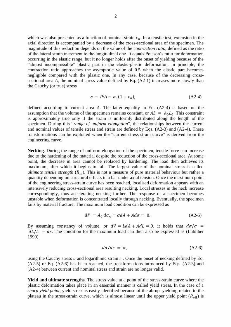
2

which was also presented as a function of nominal strain . In a tensile test, extension in the

axial direction is accompanied by a decrease of the cross-sectional area of the specimen. The

magnitude of this reduction depends on the value of the contraction ratio, defined as the ratio

of the lateral strain increment to the longitudinal one. It equals Poisson’s ratio for deformation

occurring in the elastic range, but it no longer holds after the onset of yielding because of the

“almost incompressible” plastic part in the elastic-plastic deformation. In principle, the

contraction ratio approaches the asymptotic value of 0.5 when the elastic part becomes

negligible compared with the plastic one. In any case, because of the decreasing cross-

sectional area A, the nominal stress value defined by Eq. (A2-1) increases more slowly than

the Cauchy (or true) stress

σ = P/A = (A2-4)

defined according to current area . The latter equality in Eq. (A2-4) is based on the

assumption that the volume of the specimen remains constant, or . This constraint

is approximately true only if the strain is uniformly distributed along the length of the

specimen. During this “range of uniform elongation”, the relationships between the current

and nominal values of tensile stress and strain are defined by Eqs. (A2-3) and (A2-4). These

transformations can be exploited when the “current stress-strain curve” is derived from the

engineering curve.

Necking. During the range of uniform elongation of the specimen, tensile force can increase

due to the hardening of the material despite the reduction of the cross-sectional area. At some

point, the decrease in area cannot be replaced by hardening. The load then achieves its

maximum, after which it begins to fall. The largest value of the nominal stress is called

ultimate tensile strength ( ). This is not a measure of pure material behaviour but rather a

quantity depending on structural effects in a bar under axial tension. Once the maximum point

of the engineering stress-strain curve has been reached, localised deformation appears with an

intensively reducing cross-sectional area resulting necking. Local stresses in the neck increase

correspondingly, thus accelerating necking further. The response of a specimen becomes

unstable when deformation is concentrated locally through necking. Eventually, the specimen

fails by material fracture. The maximum load condition can be expressed as

. (A2-5)

By assuming constancy of volume, or , it holds that

. The condition for the maximum load can then also be expressed as (Lubliber

1990)

, (A2-6)

using the Cauchy stress σ and logarithmic strain ε . Once the onset of necking defined by Eq.

(A2-5) or Eq. (A2-6) has been reached, the transformations introduced by Eqs. (A2-3) and

(A2-4) between current and nominal stress and strain are no longer valid.

Yield and ultimate strengths. The stress value at a point of the stress-strain curve where the

plastic deformation takes place in an essential manner is called yield stress. In the case of a

sharp yield point, yield stress is easily identified because of the abrupt yielding related to the

plateau in the stress-strain curve, which is almost linear until the upper yield point ( ) is

3

reached. Immediately after this, a rapid drop to the lower yield point ( ) is usually

observed. In this discontinuous type of yielding, significant elongation of the tensile specimen

occurs at essentially constant stress until the length of the yield plateau is reached. The

hardening stage follows the plateau with the propagating plastic deformations (cold working).

In the case of continuous yielding, hardening happens gradually, without a sharply defined

yield point. The yield stress is identified, for example, as the stress value associated with

the 0.2% permanent offset strain.

Strength data given in steel certificates are expressed in terms of the nominal stress and strain.

However, these data are directly suitable only to analysis that is restricted to sufficiently small

deformations. The yield stresses ( , and ) given as nominal values are ordinarily

quite close to those expressed in the current stresses, and they can be used with a tolerable

error in practise. In strict analysis with larger strain, the distinction between nominal and

current values must be taken into account; that is, the logarithmic strain and Cauchy stress

should replace their nominal counterparts (in structural analysis formulation). The distinction

should be made with the ultimate tensile strength ( ) commonly given in a tensile test

report, because it is usually obtained with quite a large strain value. If the associated point

( , ) of the engineering curve were known, the corresponding point of the “true stress-

strain curve” could be found through Eqs. (A2-3) and (A2-4). The value of is not usually

given in a steel certificate, and those transformations cannot be utilised without additional

conditions. The auxiliary requirement for them may be obtained through Eq. (A2-5) or (A2-

6), in the way discussed above. It is emphasized that the maximum point of the nominal

stress-strain curve is related to the onset of necking, which is the last point capable of

describing the pure material behaviour based on the used transformations. In addition, the

value for the ultimate strain ( ) and the impact toughness are usually given in the test

certificate. However, these are useless when the elastic-plastic type of hardening model is

determined.

A2.2 Curves with continuous yielding

Ramberg-Osgood model. Using the well known Ramber-Osgood formula, the virgin curve

describing hardening behaviour without a sharply appearing yield stress (and without the

following plateau) can be described as

, (A2-7)

which can be interpreted as a relationship between the logarithmic strain and the Cauchy

stress In Eq. (A2-7), E is an elastic modulus, is a reference stress, and α and n are

dimensionless constants. The (total) strain is a monotonically increasing function of stress ( )

that is divided into elastic ( ) and plastic parts ( ). The plastic

part is described by a power law type of expression with exponent n, whose inverse m = 1/n

can be identified as a work (or strain) hardening exponent as presented in Eq. (A2-8) below.

When the stress-strain curves for structural steel (with continuous yielding) are constructed

next, the starting point in this task is that the hardening exponent n is not known in advance. If

the elastic part in Eq. (A2-7) is small enough to be neglected when compared with the

plastic part , the rest of the terms represents “pure plastic flow” as

4

, (A2-8)

where C = and 1/n = m ∊ [0,1] is called a strain hardening exponent. The value

of 0 for m (n is infinite) describes the “perfectly plastic behaviour”, whereas the value of 1 (m

=1) gives, in turn, the linear dependence between the stress and strain. The value of the

dimensionless parameter n determines the steepness of the knee of the - curve as illustrated

by Figure A2-1. Typically, the plastic part remains small until and increases rapidly

when . Although there is always a nonzero plastic part in Eq. (A2-7), it is negligible up

to some stress value such that R-O model can be replaced by the linear elastic approximation.

If a curve defined by Eq. (A2-7) passes through point = ( , there is a

strain offset , which represents a permanent strain after the complete removal

of the stress. As a consequence, only one remaining parameter is needed to define the R-O

model completely, which is the exponent n. It can be solved as

(A2-9)

by requiring that the curve of Eq. (A2-7) pass through another point = . One must

keep in mind that both points and used to define the R-O model should be expressed in

terms of the Cauchy stress and Lagrange strain, unless the strain values are small enough that

the distinction between nominal and current values is insignificant.

Figure A2-1. An example of the Ramberg-Osgood model with the reference stress

with 0.2% offset. The effect on the model of increasing exponent is illustrated.

5

Determining the stress-strain curves. The objective now is to construct the stress-strain

curve with continuous yielding based on general knowledge of the elastic properties of

structural steel and data available in the test certificates. Usable data is listed below:

Elastic modulus .

0.2% proof stress obtained by a tensile test and defined as nominal values. The

associated Cauchy stress and logarithmic strain can be obtained through formulas (A2-

3) and (A2-4) deviates from slightly. It should be noted that nominal values are

sometimes used directly instead of strict values of the reference stress and the

related strain .

Ultimate tensile stress , which is determined as the maximum nominal stress value

obtained in a test. The distinction between the nominal and current stresses must be

taken into account because of the large strain related to Rm. However, the Cauchy

stress and logarithmic strain cannot be obtained through (A2-3) and (A2-4), because

the associated nominal strain value is not given in the test certificates.

The values of and are usually given in the inspection document for steel. Then, two of

the three parameters required to define the stress-strain curve, which has the same shape as

the associated R-O model, are already known or can be calculated easily (E, ), whereas the

value of the exponent n is unknown. It cannot be obtained directly through Eq. (A2-9),

because no point P2 in the (current) stress-strain curve is known. As an additional condition

related to ultimate tensile stress, the maximum load condition of Eq. (A2-5) can be employed

when the right curve is sought. This condition can be replaced by Eq. (A2-6), which is

sometimes easier to use in practice because of the shallowness of the engineering curve near

the ultimate point. Obviously, there exists an unambiguous - curve defined through Eq.

(A2-7) for every value of n. Thus, by changing the value of n, it is possible to find the right

curve satisfying Eq. (A2-5), or Eq. (A2-6) when = Rm. The problem can be given in the

form

Find parameter n such that max[ = Rm., (A2-10)

which can be solved, for example, by trial and error. The subscript of the nominal stress

does not refer to the parameter n. It is emphasized that the maximum nominal stress (or

maximum point) dictates the shape of the curve defined by Eq. (A2-7) through Eqs. (A2-5) or

(A2-6). For example, it is possible to utilize the “goal seek operation” under “what if

analysis” available in well-known Microsoft Excel-program to check whether the condition

max[ is true for the specific value of the parameter n. The strain value at the

maximum point of the stress-strain curve is achieved as a “secondary result” by the

procedure. The associated point P2 = in the “fitted R-O curve” of type Eq. (A2-7) can

be calculated subsequently. This situation is illustrated by Figure A2-2, in which both the

nominal (engineering) and the constructed curve are drawn using the same scale for the

nominal and current values (Cauchy and logarithmic) of the stresses and strains. Point P2 is a

normal point in the monotonically increasing (fitted) R-O curve, although it corresponds to

the maximum point in the engineering (nominal) curve. Transformation of Equations (A2-3)

and (A2-4) is not valid after the onset of necking.

6

Figure A2-2. Constructed stress-strain curves in the illustrative figure.

In Abaqus (Standard), the Cauchy stress and logarithmic strain were employed when the

stress-strain curves were defined. The *ELASTIC and *PLASTIC* options (Abaqus 2010)

were used, and, consequently, the material is assumed to be linear elastic up to the stress

level, where the plastic part of the strain was still negligible. The error caused by this

assumption can be restricted to be smaller than the selected tolerance value. Consequently,

without considerable error, the values of Young’s modulus E and Poisson’s ratio ν describes

the material behaviour up to the certain limit in a considered material point.

Discussion. In the R-O model, the total strain is decomposed into elastic and plastic parts: the

latter one is negligible at the beginning of the curve and prevails in the large strain values.

This decomposition applies strictly to the logarithmic strain but only approximately to the

engineering one. This difference must be taken into account when the strain is greater than

about one percent after which the model should be constructed between the logarithmic strain

and Cauchy stress to obtain a formally correct constitutive description from the plasticity

theory point of view. In the range beyond the onset of necking the pure material behaviour

can be predicted by the R-O model, which represents the monotonically increasing stress-

strain curve. It is emphasized that Cauchy stress increases monotonically according to the R-

O model, whilst the engineering stress-strain curve is descending. If the “second point” (P2),

were known in advance, the determination of the (current) stress-strain curve would be

straightforward based on Eq. (A2-9). If the value of the strain-hardening parameter is missing,

an option then is to determine this paremeter iteratively based on the conditions (A2-5) or

(A2-6) such that the maximum value of engineering stress ( ) is the strength . In spite of

the fact that the above-described iterative procedure is based on the general reasoning on the

role of the onset of necking in the tensile test specimen, it has not been widely used in

7

engineering, perhaps because of the required iteration for the value of . However, this

method is attractive when the material model must be built up through knowledge given in

inspection documents; that is, when the stress-strain curve is lacking.

The R-O formulation has been employed more commonly in the constitutive descriptions of

other metals rather than structural steel. For example, an enhanced full-range stress-strain

curve based on the R-O model for stainless steel alloys is suggested by Rasmussen

(Rasmussen, 2001; 2003a; 2003b). The value of the strain hardening exponent in is obtained

by the method of trial and error. Rasmussen’s idea was propose the stress-strain curves

based on data given in the material certificates, which is also the intention in this study.

Similar ideas as Rasmussen were also published (Mirambell et al. 2000) and discussion about

the theme appears also in the papers (Real 2003; Rasmussen 2003b). Due to the good

reliability of the test certificates nowadays, the procedures of this kind are an attractive option

in the advanced engineering analysis.

A2.3 Curves with discontinuous yielding

The segmental form of the curve is required in the description of the discontinuous yielding

behaviour with a yield plateau. This kind of presentation was exploited, for example, in an

analysis of hot and cold rolled carbon steel pipes (Xu et al. 1996). The missing data can be

completed in accordance with the results of the SINTAP (Structural INTegrity Assessment

Procedures for European industry) project ((Bannister 1998), (Bannister et al. 2000)).

The yield point phenomenon observed in a tensile test is related to a sudden and significant

amount of stretching in a plateau, which occurs at essentially constant stress once the initial

yield point ( = higher yield stress) has been obtained. However, the specimen yield stress

is usually somewhat lower ( = lower yield stress) than the initial yield stress.

Discontinuous yielding is typical for low-carbon steels (0.16–0.3% carbon). In the SINTAP

report and the related article (Bannister 1998; Bannister et al. 2000), guidance is given

regarding whether the continuous or discontinuous yielding behaviour is relevant for a certain

steel material. The likelihood of a sharp yield point decreases when the yield strength

increases. However, many other factors, including metallurgical ones, have an influence on its

occurrence and on the length of the plateau. For example, the steel composition, the

processing route in the fabrication of a steel product and heat treatments are important for this

assessment. Any process involving plastic deformations, such as temper rolling or cold

forming, may remove the yield point otherwise present in the behaviour of the used steel. In

any case, the occurrence of the yield plateau (and its length) affects the structural behaviour

substantially.

Based on the SINTAP report, the lower yield stress can be estimated by

, (A2-11)

where the coefficient corresponds to the 50th

percentile with a collation of the tensile test data

for 219 steels with yield points. Moreover, a simple formula

0.0375(1- ReL /1000) or for ReL > 1000 MPa (A2-12)

8

can be used in the prediction of the length of the yield plateau. Eq. (A2-12) gives the best-fit

estimate based on the data used in the “SINTAP project”. According to Eq. (A2-12), the

larger the yield stress is, the smaller will be the strain (Lüder’s strain). After the phase

associated with the yield plateau in a tensile test, a ductile material goes through the strain

hardening phase, where it is strengthened by the propagating plastic deformation; that is, it is

hardened by cold working. In principle, this phenomenon can be approximated by a power

law type of expression exploited in the R-O formula. It is noted that estimation schemes to

evaluate the strain hardening exponent are also suggested by the SINTAP project (but not

used in this work). Values of the strain hardening exponent for the specific steel materials

(grades) can be found in the related report (Ruiz Ocejo et al. 1998), where the stress-strain

curves are also presented.

Segmented model. In the case of discontinuous yielding, the behaviour of the ductile material

can be presented in three phases (Xu et al. 1996):

(A2-13)

written directly for the logarithmic strains and the Cauchy stresses . Their relation is

described as 1) the linear elastic phase ( , 2) the phase associated with the yield

plateau ) and 3) the strain hardening phase . The segmented

model is illustrated in Figure A2-3. When the elastic part has ended with a sharply defined

yield stress at point A , the stage associated with the yield

plateau starts. Depending on the value of exponent , the stress grows monotonically, more

or less slowly in this region up to point B . The exponent would grow very large

when almost perfectly plastic yielding is approached. The horizontal response

( , representing perfect plasticity, is not desirable due to the problems related

to the elastic-plastic solution. Finally, in the third phase, substantial strain hardening is

introduced depending on the value of the exponent . Naturally, this value should be fitted to

the actual material response. Whenever discontinuous yielding may have a role in the

structural response, it should be taken into account in the shape of the stress-strain curve. The

segmented type of model defined by Eq. (A2-13) can be exploited in the analyses including

fracture assessment (Xu et al. 1996; Wang et al. 1987). In this study, the curves with

discontinuous yielding are utilized in the elastic-plastic analysis.

Determining the stress-strain curves. The process of constructing a stress-strain curve as a

segmented model, based mainly on data available in an inspection certificate in addition to the

data obtained in the SINTAP project, is described next:

The elastic phase (defined by E and ν) is assumed to extend to stress value σ = ReL,

when ReL can be obtained by (A2-11). Point A of the current stress-strain curve

shown in Figure A2-3 represents the end of the elastic phase. Point A is very near the

corresponding point in engineering curve, such that the former of them can be

replaced approximately by the latter.

9

It is assumed at first stage that the current stress-strain curve is monotonically

increasing, such that the nominal (engineering) stress remains constant in the second

phase associated with the yield plateau. Then, the strain at the end point of the plateau

can be determined after the length of the plateau is first approximated through (A2-

12). The stress value in point B of the current stress-strain curve can be calculated by

transformation between nominal and current values. For simplicity, this relatively

short phase (second segment) can be replaced by the straight line with positive slope

connecting points A and B without considerable error. The value of the slope can be

calculated, if wanted, as the associated quotient between points A and B. The value of

the exponent is no longer needed. It is possible, in theory, to vary the length of the

plateau in order to find its proper value by comparing the FE analysis results with the

experimental data on the structural response. However, no parametric studies of this

kind were accomplished in this thesis.

The starting point of the strain hardening phase is known as the end point of the

preceding phase. The value of parameter , needed to define the third segment

, can be determined by the method of trial and error based on the task

presented by Eq. (A2-10). The prerequisite for this is, naturally, that the value of

ultimate strength , which is given normally in the test certificate, is known and

understood as the maximum point of the engineering stress-strain curve. It is

emphasized that point is “a usual point” in the monotonically growing

hardening phase of the (current) stress-strain curve (Figure A2-3).

Figure A2-3. Typical segmented stress-strain curve with three phases.

Remarks. The formulation based on R-O model or segmented model were employed by

fitting them to this discrete type of data. In the case of the segmented model, the

discontinuous yielding behaviour was taken into account, but uncertainty about the right

shape of the curve is greater here than in the case of continuous yielding. The length of the

yield plateau, and even its occurrence in the real structure, may be doubtful. The yield plateau

10

is dependent on many factors, including heat treatment and cold working of the steel and even

the manufacturing process. In tensile tests, even the testing conditions can affect the presence

and character of the yield plateau; the high stiffness of the testing machine, the high loading

rate or the possible stress concentrations in a specimen favour the formation of continuous

yielding or, at least, shorten the length of the plateau. Also, the heating cycles, such as those

caused by welding in the HAZ (heat affected zone), may lead to a continuous stress-strain

curve, although the stress-strain curve of the parent material would have been originally

discontinuous. Thus, if the yield plateau is observed in a tensile test originally, it is not

inevitably present in an actual structural component of that material, and the length of the

yield plateau may vary considerably

A2.4 Stress-strain curves of the splice parts

In the elastic-plastic simulation of an end-plated tube splice under monotonically increased

bending, the propagating plastic deformations of the bolts and end plates decrease the

stiffness of the splice gradually, such that the load-deflection curve finally turns horizontal.

For the description of the development of this kind, the elastic-plastic model of the specimen

is sufficient. Realistic stress-strain curves for the end plates and bolts are obviously required

in order to properly simulate the elastic-plastic behaviour of the arranged tests. Discontinuous

yielding with sharply defined yield stress was related only to the end plates, which were cut

from the hot rolled, normalised grade S355K2+N plates (in three delivery lot). Continuous

yielding was more likely to appear in the other splice parts than the end plate. Although a

discontinuous stress-strain curve is also typical for the base material of grade S355J2 used in

the fabrication of the tubes CFRHS250x150x10, the final stress-strain curve of the tube

presumably does not display the sharp yield point because of cold forming. The bolts made of

high-strength steel undoubtedly stand for the continuous type of material response. The

behaviour of the tubes and welds could be modelled, in principle, more roughly because of

their passive role in the specimen. The weld material is described like the material in the tube

for the FE analysis of splices. It should be noted that the changes in the (HAZ) areas, where

the material properties may have been affected by heat due to welding, were omitted in the

end plate. The stress-strain curves were determined for all splice parts according to the

procedures introduced above. It should be noted that typical stress strain curves for many steel

grades can be found in the literature (Ruiz Ocejo et al. 1998; Atlas of stress-strain curves

2002). Tensile tests results on grade 10.9 bolts at room temperature T=20 °C has presented by

Steurer (Steurer 1996).

A) Parts with continuous yielding. First, the stress-strain curves for the splice parts with

continuous yielding behaviour are constructed employing the formulation of the R-O model

presented in Eq. (A2-7). The elastic modulus = 210 000 MN/m2

was adopted (EC3).

Bolts, nuts and washers. For the bolts (M20-10.9-L70), the ultimate tensile strength (Rm)

was obtained as a mean value based on three tests. Because no measurement of strain was

arranged in these tests, the value of remained unknown. It was evaluated as

, where the nominal value of 0.9 for the ratio between yield stress and ultimate tensile

strength was replaced by the value of . It is noted that the value of ratio

typically varies in the range of 0.8 to 0.95 for high-strength steels with yield strength

up to 1000 N/mm2 (Bannister & Trail 1996). On the other hand, the higher values of the

ultimate elongation are also measured for in the tensile tests rather than for the “first-

11

generation” high-strength steels (Bannister et al. 2000). Parameter n (inverse of strain

hardening exponent) was determined for the bolts by the method of trial and error according

to Eq. (A1-10). Its value, Cauchy stress and logarithmic strain in points P1 and P2 are given in

Table A2-1. The constructed (current) stress-strain curve, which is based on the R-O model, is

shown in Figure A2-4. It is emphasised that the nominal (or engineering) curve, also shown in

the figure, is obtained by transformations that are the reverse of the constructed one. They

deviate from each other with increasing strain. The nominal curve has been drawn only up to

its maximum point, after which the transformations of Eqs. (A2-3) and (A2-4) cease to be

valid. Nuts and washers are also made of 10.9 steel, and the same stress-strain curve was used

for them as for the bolts.

Tube and weld. Based on the inspection certificate of the associated delivery lot of the tubes,

the yield stress and the ultimate tensile strength Rm were obtained for the tube material.

The reference stress is directly , and the n was determined, again, through the

method of trial and error in the task defined by Eq. (A2-10). The points P1 and P2, as well as

the value of the exponent , are given in Table A2-1. The associated stress-strain curves for

the tube are shown in Figure A2-4. The tube and weld material were assumed to have the

same stress-strain curve constructed for the tube. As noted above, the influence of welding on

steel properties was omitted.

Table A2-1. Points P1 and P2 in the R-O curve and the value of the hardening exponent.

Part Grade

%

[N/mm2]

%

[N/mm2]

n

Bolts 10.9 0.705 1061 4.25 1182 27.0

Tube (+ weld) S355J2H CF 0.432 487 5.61 581 18.7

Figure A2-4. Constructed and nominal stress-strain curves for the bolts and tube.

12

B) Parts with discontinuous yielding. Segmented model is relevant for the end plates made

of non-alloyed structural steel without cold-working.

End plates. In Table A2-2, the values of and estimated with Eqs. (A2-11) and (A2-

12), in addition to data available from the inspection certificate of type 3.1, are given to the

end plates (Table 3-3). Based on these values, the segmented curve of the type shown in

Figure A2-3 can be constructed as presented above. The elastic region ends when the nominal

stress and strain are, respectively, and . Point A of the segmented model

can be determined through the transformations (A2-3) and (A2-4), which give and

in this case because of the small strain values (the calculations are still made

correctly). In the nominal stress-strain curve, the plateau is assumed, to be horizontal with a

length of estimated by Eq. (A2-12). The end point of the second phase (B) of the

segmented curve can then be calculated through transformations of Eqs. (A2-3) and (A2-4).

Then, the plateau of the constructed curve is simply replaced by the straight line connecting

points A and B. In order to define the strain hardening segment of Eq. (A2-13), the hardening

parameter can be obtained by solving the associated problem of Eq. (A2-10). The required

data include the value of in the point at which the derivative of the nominal stress-strain

curve disappears (i.e., the onset of necking in the tensile specimen). Point C is “a regular

point” in the monotonically increasing stress-strain curve between the Cauchy stress and

logarithmic strain. The stress-strain curves are shown in Figure A2-5 for the end plates

belonging to the delivery lots with 10 mm, 15 mm and 20 mm plate thicknesses. The assumed

engineering curves defined for nominal stresses and strains are not shown in this figure,

because they do not give any additional information besides that which has already been

explained above.

Because of the lack of the actual stress-strain curve, the value of Lüder’s strain was

estimated coarsely. To shed light on the situation, three alternative stress-strain curves were

constructed for the 10 mm plate when = 1%, 2% and 3 as shown in Figure A2-6. The stress

values obtained are approximately equal for all curves when the strain is about 23%. On the

other hand, the absorbed energy (the area between the curves) related to the same strain value

might be quite different depending on the curve that is followed. However, only the selected

stress-strain curves (with Lüder’s strains given in Table A2-2) are exploited in the analyses of

the considered splices, and no parametric studies in which the related solutions for different

values of Lüder’s strain were performed.

Table A2-2. Data for the segmented models for the end plates (in nominal values)

= originally given in Table 3-3

End plates of grade S355K2+N, three delivery lots

Plate

(Inspection certificate of type 3.1) Eq. (A2-11) Eq. (A2-12)

ReH*

[MN/m2]

Rm*

[MN/m2]

ReL

[MN/m2]

[%]

10 mm 429 582 408 1.63

15 mm 378 532 359 1.76

20 mm 380 564 361 1.76

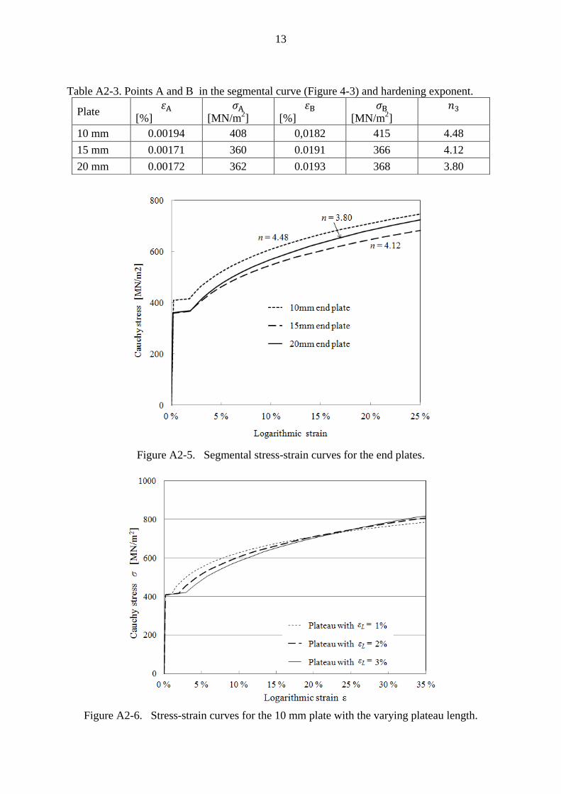
13

Table A2-3. Points A and B in the segmental curve (Figure 4-3) and hardening exponent.

Figure A2-5. Segmental stress-strain curves for the end plates.

Figure A2-6. Stress-strain curves for the 10 mm plate with the varying plateau length.

Plate

[%]

[MN/m2]

[%]

[MN/m2]

10 mm 0.00194 408 0,0182 415 4.48

15 mm 0.00171 360 0.0191 366 4.12

20 mm 0.00172 362 0.0193 368 3.80

1

APPNEDIX A3

CONTACT MODELS AND ANLYSIS METHODS

A3.2 Contact constraints ....................................................................................................... 1

A3.3 Approaches to contact description ............................................................................... 3

A3. 4 Contact constraint enforcement methods .................................................................... 4

In this appendix, the basic concepts used in contact modelling and analysis of tube splices are

discussed. The classical contact model with frictionless normal contact and non-penetration

requirement was embedded in the FE model for contacts between the end plates. The shear

tractions in the contacted surface are neglected, whilst only normal ones are transferred from

one deformable body to another. Contact analysis models and methods intended especially for

FE simulations are described by Kloosterman (2002). A compact presentation about the

procedure through which the contact problem is embedded in the virtual work equation,

defined as the basis for the discretized model in FE method, is given by Bathe & Bouzinov

(1997). It should be noted that mentioned article can be read in the context of the general FE

formulations presented by Bathe et al. (1975). Contact analysis methods available in Abaqus

are described in Abaqus manual (Abaqus 2010). However, this manual is more readable, for

example, on the light shed by the dissertation written by Kloosterman (2002). Practical advice

on how to undertake a contact and friction analysis is given in a guide published by the

International Association for the Engineering Modelling, Analysis and Simulation

Community, known briefly as NAFEMS (Konter 2000). The definitions and concepts

commonly used in contact mechanics can be found in the textbook (Kikuchi et al. 1988).

A3.2 Contact constraints

Let be the traction at a point on the surface of body I caused by the contact between bodies

I and J in the associated contact surface. The vector is defined per unit area and can be

divided by decomposition

(A3-1)

into normal and tangential components and , respectively, as demonstrated in Figure A3-1.

The directions are defined through the unit outward normal and unit tangential vector on

surface I. According to Newton’s third law, there should be an equal and opposite traction on

surface J such that . If there is no friction between the surfaces in contact, the

tangential component disappears and the “frictionless normal contact” prevails. Two material

points of a continuum cannot occupy the same location at the same time, which concerns both

interior and boundary points of continuous bodies. In contact analysis, in addition, it is

sufficient to ensure that no boundary point of a body can penetrate to another body through its

boundary. The impenetrability constraint can be defined through an inequality condition g ≥

0, where g is the normal distance from the considered point on surface I to the boundary on

the body J (Figure A3-1). The normal component of the traction must be compressive

(i.e., negative) when the positive direction is defined according to the associated outward

2

normal (vector) of the surface. The normal contact represents the classical type of interaction

given through the constraint (Kikuchi & Oden 1988; Kloosterman 2002),

, , (A3-2)

where the first two conditions were explained above and the third condition states a

complementary condition: if there is no contact ( ), then it must be the case that ; if

there is a contact ( ), then . The potential points in the - plane are shown by the

thick lines in Figure A3-2. The complementary condition is known as the Karush-Kuhn-

Tucker inequality type of constraint in the optimization problems. It should be noted that the

compressive normal component (i.e., contact pressure ) is sometimes defined as positive,

deviating from the agreement here. The constraint of Eq. (A3-2) represents the physically

“strong formulation” of the contact as such, and it should be fulfilled at every point in the

possible contact area. The “weak formulation” can be obtained when the principle of virtual

work is applied to the structural problem, including contacts, in a discrete way, for example,

in the context of the FE formulation. In a, FE model, the requirements of the contact

constraint are adopted through the nodal points (nodes) in the boundaries. The “hard contact”

characterised by Eq. (A3-2) is sometimes sought through a model where the traction is

presented as a function of the distance g, such that the latter one is then interpreted as a

fundamental unknowns describing the contact.

When the state of a normal contact is detected, the distance g between a considered point on

the slave surface and its nearest point on the master surface can be determined first. It is

advantageous to provide a smooth distance function defined everywhere on the slave

boundary when the convergent solution for a contact problem is sought. Usually, the harder or

larger counterpart of the contacted boundaries is defined as a master. The selection of the

slave and master surfaces may have a crucial influence, for example, on the convergence

(rate) obtained by the numerical solution procedure (Abaqus 2010).

Figure A3-1. a) Distance g > 0 between two bodies and b) contact traction vector when

contact is active (g=0).

3

Figure A3-2. Constraint/interface condition for normal contact ( ) without penetration

called hard contact in Abaqus Standard.

Frictional effects can be included in the contact analysis by presuming an isotopic Coulomb

model. The associated frictional constraints based on Coulomb’s friction are presented, for

example, in Kloosterman’s dissertation (2002). According to Coulomb’s law, no slip occurs if

the value of the tangential component of the contact traction is less than the critical value

, which is proportional to the normal component . The coefficient μ is known as the

friction coefficient. The related auxiliary conditions state that there is no slip if the tangential

traction has not reached its maximum. The tangential traction is constrained to work opposite

to the direction of slip. In theory, extended laws for tangential contact can be introduced when

the friction coefficient is assumed to be a function of velocity and/or pressure. For example,

Abaqus provides the Coulomb friction model in both its classical and extended forms.

A3.3 Approaches to contact description

The specialised contact elements were not used in the FE models in the analyses performed.

Instead, the “contact description” was related directly to the discretization of the deformed

bodies, including the boundaries potentially in contact (surfaces). Movements of the nodes in

the slave surface relative to the master surface were followed. The contact status of each node

was determined in accordance with the impenetrability constraint. In traditional node-to-

surface formulation, it is required only that the slave nodes do not penetrate into the master

surface, whereas the nodes of the master surface may penetrate into the slave surface. In this

context, the slave surface is seen as a set of nodal points without more detailed information

about geometry of this surface. In surface-to-surface formulation, the shapes of both the slave

and master surfaces are taken into account (Abaqus 2010). Then, the contact constraints are

enforced in an average sense over the region defined nearby considered (slave) node rather

than only at individual node. Surface-to-surface discretization usually provides better results

on the contact pressure compared to node-to-surface discretization. This is mainly due to the

fact that, in the node-to-surface formulation, forces tend to concentrate on slave nodes

because their penetration into the master surface is simply prevented (without considering the

geometry of the slave surface). In fact, the formulation based on the surface-to-surface

approach causes a smoothing effect on the nodal force distribution. With the node-to-surface

formulation, more refined meshes are usually needed to obtain equally accurate contact

pressure distribution compared to the case of surface-to-surface formulation by FE solution.

Of course, as the mesh in the contact area is refined, more accurate results can be achieved

regardless of whether the node-to-surface or surface-to-surface formulation is used. The

4

checking of the convergence in the case of the numerical model including contacts was

embedded into the convergence tests in the model of the tube splice in tension described in

Section 5. Traditionally, linear elements are used and quadratic elements are avoided when

the contact problem has been embedded in the analysis. It is true that some second-order

elements are not suitable for contact analysis when it is based on the node-to-surface

formulation. In this case, physically ambiguous distributions of nodal forces related to

quadratic elements may appear. For example, constant pressure on the contact surface

produce equivalent nodal forces, interpreted as tensile, in corner nodes (of an element) despite

these nodes should locate inside the compressed area. In contrast, the exploitation of quadratic

elements provides, in addition to higher accuracy and better ability to interpolate variables,

the possibility for stricter geometry definition with curved geometries. When quadratic

elements are used, the surface-to-surface approach must be chosen, whereby the above

complication can be avoided.

The “tracking approach” is needed when arbitrary relative displacements between two

surfaces potentially in contact may occur. The interactive surfaces may make contact and

separate, or they may rotate and slide in regard to each other. In those cases, the so-called

finite-sliding tracking approach can be exploited (Abaqus 2010). On the other hand, the finite

sliding approach is unnecessary if only the small sliding happens between the contacted

surfaces. Contact constraints can then be the fixed as a small sliding contact during the

analysis, although the status of the constraints – either separated or in contact – may vary. In

principle, the small sliding approach can be used as a part of the otherwise geometrically non-

linear analysis provided that the slave node interacts with the same local area of the master

surface throughout the analysis. In the geometrically linear analysis, the infinitesimal relative

motion between the interacting surfaces is originally presumed. In the geometrically and

materially nonlinear analysis of tube splices carried out in this work, the finite sliding tracking

analysis is exploited when the contact between end plates is replaced by a contact between the

end plate and rigid plane defined in the transverse symmetry plane as explained later. The end

plate is then allowed to slide significantly in respect to the rigid plane (constrained against

rigid body movements).

A3. 4 Contact constraint enforcement methods

The formulations of contact analysis embedded in numerical models are usually based on the

principle of virtual work, through which the weak formulation can be obtained. When

applying this principle, the virtual work done by the contact tractions is simply added to the

virtual work equation describing the balance between the internal and external virtual work

done in the entire system (Bathe et al. 1997). Bathe suggest how the contact constraints can be

imposed using the contact constraint function method. This method is not used in the analyses

done for this study by Abaqus, but it is briefly explained in order to shed light on the

character of the contact analysis. In the used numerical solution procedure, the contact

constraints embedded in the structural analysis problem are enforced through the contact

constraint enforcement method. The used procedure is explained in Abaqus manual but

perhaps in more understandable way in Kloosterman’s dissertation (2002).

In the contact constraint function method, the inequality type of constraints presented through

Eq. (A3-2) is replaced by an equality type of constraint (Bathe et al. 1997):

, (A3-3)

5

where is a continuous and differentiable function of clearance g and contact traction

(see Figure A3-1). Moreover, the contact constraint function is defined such that

this otherwise nonzero function has a zero value only when the constraint of Eq. (A3-2),

illustrated by Figure 4-9, is satisfied. It must be adequately regular in order to avoid numerical

complications in the solution procedure, which consists of solving the associated virtual work

equation when the equality type of constraint given in Eq. (A3-3) is imposed. This can be

done using, for example, the Lagrange multiplier method, which provides a traditional way to

solve a problem including constraints. In any case, the solution is sought for the discretised

model accompanied by a finite number of variables, including those related to the nodal

points in the contacted areas. By the Lagrange multiplier method, the contact constraints are

enforced strictly at the related nodes of an FE model. If the contact traction is introduced as

a Lagrange multiplier, the mixed type of formulation with both spatial variables (which are

defined in the displacement-based FE formulation used) and force variables is used. The

Lagrange multiplier method has a disadvantage in that the number of degrees of freedom is

increased by it.

In the penalty method is classified under the framework of regularisation methods

(Kloosterman 2002). Contact traction is presented as a function of the related normal distance

(clearance or penetration, if negative) with which it forms a conjugate pair in the work

equation. The solution is sought by allowing violations of the contact constraints in order to

estimate the direction and magnitude of the tractions. The penetration is defined as a measure

of the violation of the impenetrability constraint. The idea is to penalise this violation of the

original constraint such that, the larger the penetration is, the larger the resistance to it will be.

The violations of the originally assessed constraints can be fully eliminated, in theory, only if

the penalty parameter (which physically represents the stiffness) goes to infinity. On the other

hand, the large penalties may unfortunately cause numerical instability. The accuracy depends

decisively on the value of the penalty parameter, which also determines the severity of the

violation. Usually, it is possible to achieve a tolerable approximate solution of a contact

problem through a sufficiently large penalty parameter by the penalty method. The

discontinuity character of the original contact problem is avoided due to the penalty method;

therefore, it is more suitable (regular) for use with continuum formulations. In principle, the

penalty method can be included in the iterative scheme through which the violations of the

constraints (i.e., penetrations) are driven down. The iterative method of this kind, called the

augmented Lagrange method, is usually more preferable to use than the plain penalty method.

The contact tractions achieved in the current step can be interpreted as estimates of the

Lagrange multipliers. A repeated step gives a more accurate solution to the contact problem

and improves the estimates of the Lagrange multipliers compared to the preceding step.

Contact constraint methods in Abaqus Standard. There are three contact constraint

methods available in the used version of Abaqus Standard: the direct, penalty and augmented

Lagrange methods. Next, some aspects from these are discussed. The direct method is

associated with the Lagrange multiplier method strictly enforcing the contact constraint of Eq.

(A3-2), illustrated by Figure A3-2. Thus, the traction (in frictionless contact) is transferred

over the surface in contact without the penetration, whilst it disappears entirely if the

clearance between the surfaces is nonzero. If the clearance reduces to zero, the separated

surfaces come into contact. The direct method can also be used to enforce “softened contact

behaviour” based on the softened relationship between pressure and the associated

overclosure (penetration). It is emphasised that the softened contact behaviour is not exploited

1

APPENDIX A4

FE SIMULATIONS: CONTACTS AND PRYING ACTION

A4.1 Splice model ................................................................................................................ 1

A4.2 Comparisons between contact analysis methods ......................................................... 3

A4.3 Contacts caused by pre-tensioning and prying ............................................................ 5

A4.3 Splice response during necking ................................................................................... 6

The role of contacts in the response of tube splices is clarified by describing the results of the

elastic-plastic FE analysis of a tube splice under axial tension, which represents a problem of

type II classified in Section 2.2.7. The contact analysis is embedded in the analysis of the 3D

FE model on the considered tube splice. The structural model and its discretization are

described in greater detail in Section 4.2.3. In this appendix, the focus is on the results of the

analysis. Contact between the end plates, which is replaced by the contact between the end

plate and the rigid plate coinciding with the transverse symmetry plane. It will be described

how contacts are changing from those caused by pre-tensioning of the bolts to those caused

by external loading (enforced displacement). The response of the splice is followed beyond

the point at which maximum axial force is obtained to the descending stage of the load. The

character of the prying action throughout the loading can be demonstrated by this example.

A4.1 Splice model

The considered splice in axial tension is assumed to have structural symmetry in respect to

three planes, as demonstrated in Figure A4-1. Thus, it is sufficient to consider only one eighth

of the tube and its splice, which are shown in an oblique view in Figure A4-3. The specific

geometry of the splice and its material properties are defined as those of splice S1, studied

through tests TE1 and TE8 (Table 3-3). The dimensions can be found in Figures 3-3 and 3-4,

and the material definitions are presented in Section 3.2.2. The stress-strain curves for the

steel parts of the splice are constructed in Appendix A2, where the associated parameters are

given in Tables A2-1 and A2-3. The incrementally increased axial elongation 2 is

introduced to the tube and its splice in order to define the problem of the splice in axial

tension. Because of the displacement controlled solution procedure, also the stage of the

descending axial load can be followed. The axial force can be assumed to be distributed

evenly over the tube cross-section at the ends of the tube. It is emphasised that the reduced

1/8-model can be identified as a tension component of the component method (Appendix A5)

for a quarter cross-section of the splice with a single bolt in the end plate corner.

Contact between the end plates (A), which plays the key role in the splice behaviour, was

introduced as frictionless normal contact between the end plate and the rigid surface at the

transverse symmetry plane, in compliance with the constraint condition of Eq. (A3-2) of

Appendix A3. The transverse symmetry plane is defined as the master surface, whilst the end

plate acts as the slave surface. A fastener comprising a bolt, a nut and washers is introduced

as a monolithic part (model B2 in Figure 4-9), which is symmetric in respect to the transverse

plane at mid-span. Accordingly, internal contacts (B and C in Figure 4-2) have been omitted

based on the assumption that they have no essential influence on the global response of the

considered splice under either axial tension or pure bending. Contacts between the washer

2

and end plate (D) are replaced by the constraint, which allows for no relative movement

between the surfaces in contact. This can be done through the “surface based TIE constraint”

available in Abaqus. In TIE constraint, the slave nodes that initially are in contact with the

master surface will be tied to it throughout the analysis, whilst those nodes in the slave

surface, which are not constrained, can move independently of the master surface (i.e., these

nodes never see the master). The pre-loading force of the bolt was either assumed to be B0 =

99.4 kN, which is the same as in test TE7 but not in test TE1 with lower pre-tension (Section

3), or it was neglected (no pre-tension). In the latter case, a small bolt force with no essential

influence on the splice behavior was used because of easy treatability of the results.

The (discrete) model of the splice in axial tension is introduced in Section 4, where the

boundary conditions and the loading caused by the enforced displacement are explained. The

contact problem was embedded in the verification procedure in the elementary problem of the

splice in axial tension in the convergence tests with the coarse, medium and fine mesh. The

convergence was obtained in respect to the solved global quantities (i.e., in the resultant

level). In the next analyses, the end plate was discretised by the fine mesh. Next, the analysis

results concerning, particularly, the role of the resultant contact force between the end plate

and rigid surface at mid span are described in the splice response. Contact analysis methods

available in Abaqus are also compared with each other.

As a preparatory step of the computational procedure, contacts must first be initiated. This

can be done, in theory, with small enforced displacement that is 1) sufficient to ensure the

stability of the model through the contacts but 2) small enough not to cause plastic

deformations in the bodies it affects. In the next loading step of the analysis, the condition

used in initiation should be removed so that none of its influence remains in the final analysis

results. After initialising contacts, the bolts can be pre-tensioned (whilst the artificial

conditions are removed). Finally, the stable and preloaded splice is ready to take external

loads. For the initiation of contacts, in principle, the bolts can be shortened a little, in which

case the end plate and rigid plate are clamped together. Pre-tensioning of the bolts is also

based on a procedure of this kind; therefore, it is sometimes more practical to include the

initiation of the contacts in the step taken for pre-tensioning of the bolts. In any case, the first

step of the iteration must be small enough to obtain convergence. It should be noted that bolt

pre-tensioning is a readily available option, for example, in Abaqus.

Figure A4-1. The splice in axial tension and planes of structural symmetry (Abaqus).

3

Figure A4-2. The resultant forces defined per a quarter of the tube and its splice (this

axonometric figure is printed from Abaqus).

A4.2 Comparisons between contact analysis methods

Axial load , which is integrated over a quarter of the tube cross-section, can be obtained

easily from the results of the elastic-plastic 3D FE analysis for the incrementally increased

elongation ( ). The (symmetric) boundary conditions for the bolts are described

independently of those given for the rigid surface at mid-span. Then, the resulting contact

force (defined consistently with ) between the end plate and rigid surface is obtained

directly as the axial reaction force at the arbitrarily placed support preventing the rigid body

motion of the rigid surface. There is a bolt at every symmetric quarter of the splice, and the

force per bolt must be multiplied by four to obtain the total force taken by all bolts of the

splice together. It is noted that in Abaqus, the current bolt force can be readily followed in the

pre-tensioned bolts. The external force is obtained as

(A4-1)

when the equilibrium in the axial direction is required. If there is no contacts between the end

plates (or end plate and rigid surface), then the external force would be equal to the bolt

force . Contact force is due to pre-tensioning or/and the prying action: in the former, the

end plates are clamped together, while in the latter the bent end plates push each other such

that the additional bolt force develops. It should be noted that both pre-tensioning and prying

action are self-equilibrated phenomena. The results of the FE analysis are presented in Figure

A4-3, where all three resultant forces P, B and C are plotted as the function of the enforced

axial displacement , which equals approximately the average displacement of the splice

because of the large axial stiffness of the tube in respect to splice. The ultimate tensile

strength of the splice is obtained as

, (A4-2)

which is the maximum value of the difference instead of the strength of the bolt

. In other words, the contacts between the end plates weaken the splice from

that predicted by the strength of the bolt only. These contacts are mainly caused by the prying

effect as shown below.

4

0

50

100

150

200

250

300

0 10 20 30 40 50 60

B, C

or

P[k

N]

u [mm]

Direct method (Lagrangian multipliers)

Penalty method with augmented iterations

Penalty method

B

C

P = B - CC D

Pmax

B F

A

Cmax

Bmax

ES

In Figure 4-12, a total of nine curves obtained by three different FE analyses are drawn.

Every analysis is based on one of the three methods to enforce contact constraints (Eq. A4-2)

presented in Appendix A3. These method are also available in Abaqus. The only difference

between these analyses and, consequently, between the corresponding curves is in the

selection of the contact constraint enforcing method. Thus, there are three curves for each of

the relationships B-u, C-u and P-u in the figure. By the direct method, the weak form of the

(hard) contact is enforced strictly at the nodes, whilst the penalty and augmented Lagrange

method (i.e., penalty method with augmented iterations) give approximate results. The

solution obtained by the direct method can then be seen as a reference solution for the latter

two, although it is also an approximation for the continuous problem replaced by the discrete

one. The results of the convergence tests for the tube splice under axial tension are considered

elsewhere in the thesis (in Section 5). In any case, the corresponding curves attained by the

direct, penalty and augmented Lagrange methods are very close to each other, such that they

form a tight bundle. In this example, there was no use of augmented iterations by which the

solution obtained by the penalty method could be improved. The contact problem included in

the analysis of the splice can be characterised as smooth in nature; therefore, it was

comparatively easy to obtain an approximate solution. Moreover, no essential differences

were found between the methods used. Thus, the direct method was primarily used in the

contact analyses embedded in the numerical solution procedure in the thesis. If the converged

solutions had not been obtained through it, the augmented Lagrange method would have been

the next best alternative.

Figure A4-3. Resultant forces , and predicted by the FE model (Abaqus).

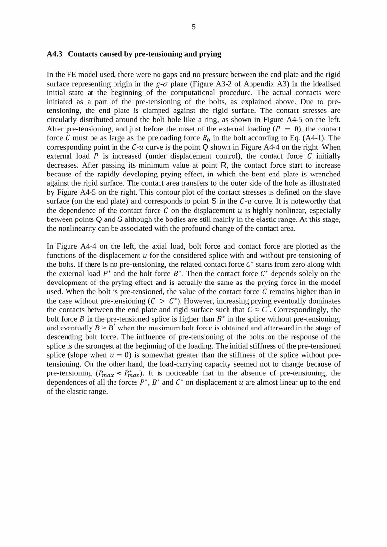
5

A4.3 Contacts caused by pre-tensioning and prying

In the FE model used, there were no gaps and no pressure between the end plate and the rigid

surface representing origin in the - plane (Figure A3-2 of Appendix A3) in the idealised

initial state at the beginning of the computational procedure. The actual contacts were

initiated as a part of the pre-tensioning of the bolts, as explained above. Due to pre-

tensioning, the end plate is clamped against the rigid surface. The contact stresses are

circularly distributed around the bolt hole like a ring, as shown in Figure A4-5 on the left.

After pre-tensioning, and just before the onset of the external loading ( ), the contact

force must be as large as the preloading force in the bolt according to Eq. (A4-1). The

corresponding point in the - curve is the point Q shown in Figure A4-4 on the right. When

external load is increased (under displacement control), the contact force initially

decreases. After passing its minimum value at point R, the contact force start to increase

because of the rapidly developing prying effect, in which the bent end plate is wrenched

against the rigid surface. The contact area transfers to the outer side of the hole as illustrated

by Figure A4-5 on the right. This contour plot of the contact stresses is defined on the slave

surface (on the end plate) and corresponds to point S in the - curve. It is noteworthy that

the dependence of the contact force on the displacement is highly nonlinear, especially

between points Q and S although the bodies are still mainly in the elastic range. At this stage,

the nonlinearity can be associated with the profound change of the contact area.

In Figure A4-4 on the left, the axial load, bolt force and contact force are plotted as the

functions of the displacement u for the considered splice with and without pre-tensioning of

the bolts. If there is no pre-tensioning, the related contact force

starts from zero along with

the external load and the bolt force . Then the contact force

depends solely on the

development of the prying effect and is actually the same as the prying force in the model

used. When the bolt is pre-tensioned, the value of the contact force remains higher than in

the case without pre-tensioning ( ). However, increasing prying eventually dominates

the contacts between the end plate and rigid surface such that C ≈ C*. Correspondingly, the

bolt force in the pre-tensioned splice is higher than in the splice without pre-tensioning,

and eventually B ≈ B* when the maximum bolt force is obtained and afterward in the stage of

descending bolt force. The influence of pre-tensioning of the bolts on the response of the

splice is the strongest at the beginning of the loading. The initial stiffness of the pre-tensioned

splice (slope when ) is somewhat greater than the stiffness of the splice without pre-

tensioning. On the other hand, the load-carrying capacity seemed not to change because of

pre-tensioning ( ). It is noticeable that in the absence of pre-tensioning, the

dependences of all the forces , and on displacement are almost linear up to the end

of the elastic range.

6

Figure A4-4 Axial forces , and predicted by Abaqus in the splice with and without pre-

tensioning. The beginnings of the curves are drawn to a larger scale on the right.

Figure A4-5. Contact stresses on the end plate (slave surface) after pre-tensioning in point Q

and point S of the C- curve in Figure A4-4 on the right (Abaqus).

A4.3 Splice response during necking

When the end plate deforms during loading, some contacts may remain whilst others cease to

exist because of the separating surfaces, and those areas in contact can slide without friction

along the rigid surface. Both the extent and the location of the contacts may change. The

changes in the contacts were described above at the beginning of the loading history. To

better understand the development of contacts between the end plate and rigid surface during

7

the rest of the loading, a series of contour plots presenting the contact stresses on the end

plate (slave surface) is shown in Figure A4-6. These correspond the configurations of the

splice at points A to F in the - curve of Figure A4-3. Point A refers to the same

configuration as point S in the - curve in Figure A4-4 on the right. Point A is still in the

elastic range, whereas point B belongs to the plastic stage of the splice response. Point B can

be seen as a starting point of the almost linear “hardening phase” of the - curve continuing

up to point E, where the maximum load is attained. Points C and D are associated

with the occurrences of the maximum value of the contact force C and the bolt force B,

respectively. In the hardening phase (from B to E), the contact area seems to move gradually

towards the outermost corner and to the end plate edges joining in the corner. At point F in

the descending phase of the - curve, contacts between the end plate and rigid surface

disappear entirely. Then, the value of the axial load P equals the value of the bolt force B.

Because of prying, the current bolt force cannot be utilised wholly in the response of the

splice, as concluded above. The prying force is increasing up to the point at which the contact

force attains its maximum value , corresponding to point C in the - curve of

Figure A4-3. The contact force decreases after this and finally disappears when the

configuration related to point F is reached. The influence of the decreasing prying on the

splice response is explained next. After point D, which corresponds the maximum bolt

force , the onset of necking weakens the splice. Surprisingly, the axial load taken

by the splice can still grow (from D to E). Then, the prying force decreases more rapidly

than the bolt force B, such that the load represented by the difference is

increasing. Eventually, the propagating necking cannot be compensated for any further by

relaxing prying, and the global response of the splice becomes unstable. It is noteworthy that,

regardless of the strongly nonlinear behaviour of the bolts and changing contacts, the

difference is almost linear in respect to the displacement u between points B and

E. Of course, the hardening has its own role in the global response of the splice.

Discussion. In the performed elastic-plastic simulation of a flanged tube splice S1 under axial

tension, the contact analyses were included, and the role of contacts in the splice response

was elucidated. The simulation revealed that, while contacts caused by pre-tensioning

initially prevailed, those produced by the prying effect developed gradually with increasing

external loading. Eventually, there were no differences between the axial forces resulting in

the splice with pre-tensioning and without it, as shown in Figure A4-4 on the left. Contacts

caused by the prying then dominated the splice response entirely. According to the elastic-

plastic simulation, the influence of decreasing (ore relaxing) prying on the splice response

could compensate for the local instability caused by necking of the bolts, such that the global

response of the splice was still increasing. This phenomenon appeared in a very late stage of

the loading and was not seen in tests TE1 and TE7 arranged for splice S1 due to the

premature termination of those tests. The importance of the phenomenon called relaxing

prying is obviously more theoretical than practical in engineering. However, the simulation

shows how the splice could behave if the ductility of the material (in the bolts and end plates)

were fully utilized. It should be noted that, in tests TE3 and TE8, where necking was obvious,

relaxing prying might have been affected the responses of the splice before their terminations.

However, the utilization of phenomena of this kind would not be reasonable in engineering

due to the brittle character of the bolts.

8

Figure A4-6. Contact stresses on the end plate (slave surface) based on the results of Abaqus

analysis in points A to F defined in Figure A4-3.

1

APPENDIX A5

FE SIMULATIONS: TENSION COMPONENTS

A5.1 Quarters Q1 to Q4 ........................................................................................................ 1

A5.2 Computed - curves .................................................................................................. 3

A5.3 Resistances ................................................................................................................... 4

A5.4 Stiffnesses, fitting procedure ....................................................................................... 5

A5.6 Bolt forces ................................................................................................................... 8

A5.7 Effect of the weld dimensions ..................................................................................... 9

A5.8 Effect of the pre-tensioning ....................................................................................... 10

In Appendix A5, the responses of the splices in axial tension are simulated. Due to the

structural symmetry of splices S1 to S3 with the corner bolts, the response of the individual

corner components can be extracted from the results (splice S4 with mid-side bolts was

somewhat complicated in this respect). The resistances, stiffnesses and bolt forces are solved

through the elastic-plastic model, which do not take into account the material fracture. From

this point of view, the obtained results are theoretical in their character. In any case, the

resistance in reserve over that predicted by the component method in respect with that

predicted by the elastic-plastic model can be determined. Thus, this reserve, which is mainly

due to the strain hardening stage in the simulated response, is demonstrated by the

comparison between the computational resistances. The stiffness formulations of the EC3 can

also be investigated on the light shed by the stiffnesses obtained by the FE simulations.

Actually, the reduction factors are determined for the (tentative) stiffness formulas of the

tension components. Of course, also this procedure has only a demonstrative value, because it

is based on the comparison between the results obtained by two computational methods

without the solid experimental basis. The influence of the varying end plate thickness on the

bolt forces is studied through the FE simulations. Finally, the effects of the weld dimension

and bolt pretension on the response of the component are considered.

A5.1 Quarters Q1 to Q4

In this appendix, the responses of splices S1 to S3 with corner bolts and splice S4 with mid-

side bolts to axial tension are considered. The models of these splices in interest have each

three reflecting planes of structural symmetry, such that the transverse symmetry plane

divides the splice into two halves, and both of these halves can be further divided into four

symmetric parts through two longitudinal symmetry planes. The formed 1/8-models are called

Q1 to Q4, which correspond, respectively, to splices S1 to S4. These “quarters” Q1 to Q4

transfer a fourth of the total axial force ( applied to the whole splice. The material

properties and geometry of the quarters are adopted from the corresponding splices, i.e., from

the specimens of the arranged tests (Section 3). As an exception, the used models may be

defined with or without pretension of the bolts. The FE meshes were defined as medium

meshes (Section 4). The quadratic element C3D20R was employed in the active (= most

deformed) parts of the FE model.

2

The FE analyses of the quarters were performed under displacement control such that the

axial displacement of the tip of the tube marked as is increased step by step for the

incremental and iterative solution procedure. The axial deformation of the tube remains

negligible in respect to that of the splice because of the large axial stiffness of the tube

compared with the stiffness of the splice. Thus, the displacement represents with sufficient

accuracy also the axial deformation of the splice. The axial force , contact force and bolt

force in the quarter can be defined as functions of displacement through post-processing

from the analysis results as explained in Section 4. By the solution strategy used, the

response could be followed without convergence problems over the maximum axial load

to (globally) unstable phase until the contact between the end plates is lost

( ). The corresponding configurations of quarters Q1 to Q3 with the corner bolts are

shown as a series in Figure A5-1. At that moment, when , the prying actions cease to

wrench the end plate and the axial load is transferred over the splice purely through the

bolts ( as explained through the simulations presented in Appendix A4. In Figure A5-

1, the associated values of are also given. It is seen immediately that the thicker the end

plate is, the stiffer is the quarter.

Figure A5-1. Deformed shapes of quarters Q1, Q2 and Q3 with 10, 15 and 20 mm end

plates, respectively, when the contact force disappears ( ).

Quarter Q4 represents splice S4 in axial tension. In the model of quarter Q4, both mid-side

bolts (marked 1 and 2) are halved along the symmetry planes, where the symmetric boundary

conditions were given at the associated intersections of the end plate, tube and bolts. The FE

analysis of quarter Q4 was performed by controlling the tip displacement in the tube end. In

Figure A5-2, the configuration of Q4 is shown at the moment when the contact force

disappears ( ). The analysis revealed that the bolt on the shorter side of the end plate (no.

3

1) and the one in the longer side (no. 2) had almost equal bolt forces up to the maximum axial

load , after which the bolt in the shorter side took a somewhat larger load. The value of ,

when , is only little larger than that calculated for model Q3 when contact between the

end plate and rigid surface is lost. Thus, splice S4 (Q4) with the flexible end plate seems to

behave approximately as stiffly as splice S3 (Q3) with twice as thick an end plate. This

implies that the mid-side bolts have greater efficiency than the corner bolts.

Figure A5-2. Deformed shape of model Q4 with the 10 mm end plate is drawn when the

contact force disappears ( ).

The stiffness and resistance of quarters Q1 to Q3 must be multiplied by two when compared

with the components defined per tension flange of splices S1 to S3 including two corner bolts

(or a bolt row). The response of quarter Q4 with the mid-side bolts represent on average value

computed for two adjacent tension flanges related to the same corner of the rectangular end

plate. If the components related to the mid-side bolts behaved independently of the side length

of the end plate, quarter Q4 could be interpreted directly as a “mid-side component”. Actually,

this simplification is consistent with the ideology of the component method and it is used as

approximate one when the results of the FE simulations of quarter Q4 are considered.

A5.2 Computed - curves

The computed - curves of quarters Q1 to Q4 are given as in Figure A5-3. It should be

noted that the force must be multiplied by four, but the related displacement is

the same when defined for the whole splice under axial tension. All curves are drawn up to

the point at which contact between the end plates (or between the end plate and rigid surface)

is lost ). Because of the missing pretension, the contact forces are caused solely by the

prying action. In model Q4, the force is divided into two bolts halved by the longitudinal

symmetry planes. Then the bolt force per corner represents a sum of two bolt forces, or

, where subscripts 1 and 2 refer, respectively, to the bolts of the shorter and

longer sides of the end plate, as shown in Figure A5-2. Furthermore, the contact force is

due only to prying related to both bolts. Next, the ultimate resistances and initial stiffnesses of

the quarters are determined from the - curves based on the elastic-plastic analysis without

the description of the material fracture. No failure caused by the material fracture in the welds

and bolts occurred in the arranged test on splices S1 to S4. Instead, the cracks that appeared in

4

0

20

40

60

80

100

120

140

160

180

200

0 10 20 30 40 50 60 70

P[k

N]

u [mm]

Q4 (11.0 mm end plate)




the strongly bent end plate may have been influenced by shear at the toe of the weld between

the tube and end plate. The “premature failure” that occurred before the maximum load of

the elastic-plastic analysis was reached was striking in the case of splices with the thinnest

end plates in the tests. Despite its restrictions, the accomplished analysis may aid in

understanding the behaviours of the splices. The focus is on the tension components, the

resistance and stiffnesses of which can be directly compared with the results obtained for the

quarters Q1 to Q4 by FE analysis. To obtain a better correspondence between the tension

components and quarters, the weld is omitted ( , see Figure A5-8) and the bolts are

assumed to be assembled without pre-tensioning.

Figure A5-3. - curves based on models Q1 to Q3 with the corner bolts

and on model Q4 with mid-side bolts in the end plate (solved without pretension).

A5.3 Resistances

The tension resistances of quarters Q1 to Q4 without pre-tensioning were determined

as the maximum loads obtained in the - curves. They are shown in addition to the related

displacement in Table A5-1, where the corresponding component resistances

defined “per quarter” (compare Table A5-7 in Section 5) and, moreover, the ratio

are given. For the series of quarters Q1 to Q3 with the corner bolts, it holds that the

larger resistance is obtained with the thicker end plate, whereas displacement

increases with the decreasing thickness of the end plate. Quarter Q4 with the mid-side bolt

took a larger load than quarter Q3, which has (nominally) twice as thick an end plate. It

should be remembered that splice S3 with the corner bolts carries, in turn, a larger load than

5

S4 with the mid-side bolts by the elastic-plastic analysis. This follows mainly from the larger

lever arm on average in the splice equipped with corner versus mid-side bolts. Premature

failure in test TE11 on splice S4 affected the resistance more than in test TE3 on splice TE8

as described in Section 4.

First the series of quarters with the corner bolts is considered. An extremely long hardening

stage can be found in the - curve of quarter Q1 (Figure A5-3) obtained by the elastic-

plastic analyses FE model after the knee point occurring at the level that roughly represents

the resistance predicted by the component method. Consequently, the smallest value of 0.61

for the ratio was then found. Of course, the large reserve in resistance predicted

by it comes through only if premature failure does not occur. The value of the ratio

is 1.02 for quarter Q3 with the thickest end plate . Thus, the resistance

predicted by the component method is about 2% larger than the predicted by

the FEA, and there is no reserve in resistance at all (or “negative reserve”). In the case of

quarter Q2 with the intermediate end plate thickness ( , the predicted behaviour

of the elastic-plastic FEA is somewhere between that observed with quarters Q1 and Q3, as

shown in Figure A5-3. The knee point in its - curve is not as sharp as in the case of Q1; on

the other hand, the hardening stage is longer than in the case of Q3, where it almost

disappears. It should be remembered that the component resistances for splices S1 and S2

belong to mode 1 whilst S3 represents mode 2. The correspondence can be seen between the

failure modes of the equivalent T-stub and behaviour predicted by elastic-plastic FEA for

quarters Q1 to Q3. As explained before in the validation of the elastic-plastic model against

the resistances observed in the bending tests on the considered splices, the premature failure

not taken into account in the FE analyses makes the main difference in the case of the flexible

end plates, whilst the resistance of the splices could be estimated better in the case of stiffer

end plates. This feature is inherited, obviously, in the analysis of the splices under axial

tension.

The assumed elastic-plastic behaviour of the flexible end plate in quarter Q4 explains the

relatively large reserve in resistance caused by the hardening after the clear knee point seen in

Figure A5-3. Comparison between quarter Q4 and splice S4 reveals, in turn, that the value of

ratio determined for quarter Q4 in tension was quite close to the ratio

(or ) of splice S4 under bending.

Table A5-1. The resistances of the quarters and the corresponding component values.

Splice/quarter

[kN]

[mm]

[kN]

Q1, mm end plate 127 54.5 77.5 0.61

Q2, 15 mm end plate 137 34.0 101 0.74

Q3, 20 mm end plate 175 10.5 179 1.02

Q4, 10 mm end plate 186 15.7 144 0,77

A5.4 Stiffnesses, fitting procedure

The initial stiffness against tension was evaluated here as a ratio based on the

first incremental step taken in the FE solution procedure. The values of for quarters

Q1 to Q4 are given in Table A5-2 and illustrated by Figure A5-4, which has been scaled near

6

the origin such that the differences in the initial stiffnesses can be distinguished. The stiffness

increases with the thickness of the end plate in the series Q1 to Q3 with the corner bolts. The

stiffness of Q4 with the mid-side bolts and the thinnest end plate, however, gave the largest

value of . The same order of stiffnesses was observed in the bending tests for splices

S1 to S4, described in Section 3 (see Figures 3-8 and 3-13). Obviously, the FE simulations for

the quarters standing for splices under axial tension can describe the essential features

affecting their stiffness apart from the initial state of the splices, including deviations from

ideal geometry, initial strains and stresses. The initial stiffnesses of Table 5-8 were

utilised as tentative values in the models formed for the analyses of the tube splices by the 3D

component method and were determined according to the formulations of the standard, as

explained above. They represent the resistance of the components against extension. In Table

A5-2, the stiffnesses marked as are defined for a corner such that they can be compared

directly to the values of of the quarters Q1 to Q4.

Table A5-2. Initial stiffness of the 1/8-models and the corresponding component.

Model

[kN/mm]

[kN/mm]

Q1, 10 mm end plate 54.1 171 3.16

Q2, 15 mm end plate 71.2 368 5.17

Q3, 20 mm end plate 102 732 7.18

Q4, 10 mm end plate 122.7* 324 3.18

= Average value of two sides.

Figure A5-4. Scaled - curves.

In the case of quarters Q1 to Q3 with the corner bolts, the ratio is larger when

the end plate is thicker, such that it is 3.15 for Q1 with the thinnest end plate and 7.18 for Q3

with the thickest end plate. Thus, the tentative stiffnesses were many times larger than the one

predicted by the FE analysis of the associated quarters. This was expected because the used

formulas of were not meant for the flanges with the corner bolts, which represent a

more flexible response than the intended case of a “flange with a bolt row” (without corner

7

bolts). The formulas are based on the simplified assumption that the bent end plate flange can

be modelled as a beam whilst the actual behaviour of the end plate flange should be analysed

as a plate problem. This difference stands out when the end plate flange with the corner bolts

is considered. To clarify the situation in the case of splices with corner bolts, the tentative

stiffness is presented in Figure A5-6 as a function of the end plate thickness in modes

1 and 2. It is shown by the figure that, in spite of the discontinuity between the parts related to

modes 1 and 2, depends roughly linearly on , which will be exploited later. In addition,

three points taken from the FE solutions for quarters Q1 to Q3 are shown and connected by

the dotted line in Figure A5-6. It can be seen that the stiffness depends almost

linearly on the thickness of the end plate. As a result, one can also suggest that the difference

- increases coarsely as a linear function of in the case of the corner bolt.

In the case of splice S4 with the mid-side bolts, the stiffness defined for a corner was

about 3.18 times greater than estimated through the FE solution of model Q4. The

used “tentative stiffness formula” predicts the initial stiffness of the flange with the mid-side

bolts in the same relative accuracy (Table A5-2) than in the case of a flange with corner bolts

in splice S1 with the same end plate thickness. Based on the comparison between the initial

stiffnesses predicted by the two computational methods, the tentative stiffness is more

reasonable for the flange with thin than thick end plates.

Figure A5-6. Tentative stiffness of the corner component as a function of and

stiffnesses of quarters Q1 to Q3 based on the FEA solutions.

The stiffness formulas for the extended part of the end plate equipped with the corner bolts

definitely need to be improved. Because of the unavoidable character of this two-dimensional

problem of the bent end plate, the related equations are cumbersome to derive. An attractive

alternative is to exploit the existing formulas of EC3 for the stiffness coefficients (Table 6.11

of EN1993-1-8) utilised above. When the correction is made directly for the resultant stiffness

, neither of the formulas required in the evaluation of the

tension component (i.e., the coefficients and , intended, respectively, for a

“bolt in tension” and an “end plate in bending”) need any reformulation. In Figure A5-7, the

ratio is expressed as a function of the ratio instead of the end plate

thickness , as follows

8

0

2

4

6

8

10

12

0 0,5 1 1,5

c 1=

Kc,

ini/K

FE

A,i

ni

t : t1

= calculated values

(A5-1)

where is defined as equal the end plate thickness when . Thus, must be

multiplied by in order to obtain the stiffness predicted by the FEA. Eq. (A5-1) is drawn by

two points associated with the end plate thicknesses of 11 mm and 20.3 mm, both of which

are combined with bolt size mm. The relation described by Eq. (A5-1) binds the

corner bolt (diameter and end plate (thickness ) together in a dimensionless way such that

it is also valid, in theory, with other (reasonable) combinations of and . Of course, the

quarter layout and material properties used were adopted from the splices associated with

tests TE1, TE2 and TE3 accompanied by the symmetrically placed corner geometry with

and (Figure 5-8, table 5-3). The distance of the bolt from the tube wall

is, obviously, an important parameter, such that also depends on it in a decisive

way. The larger is the role of the shear on the stiffness of the end plate, the closer the bolt has

been placed to the wall of the tube. Then the slope of the line describing the reduction factor

for the stiffness formula may change. The modifications and applicability of the formulas for

the coefficient would be laborious to develop, and this is not attempted here. Finally, it

should be noted that the influence of the different material properties on the initial stiffness is

limited in the elastic modulus , which is almost constant for all steel qualities typically

used in the end plates.

Figure A5-7. Stiffness ratio approximated as a linear function of the

relative thickness of the end plate.

A5.6 Bolt forces

The resistances and stiffnesses presented above were based on the FE analyses of quarters Q1

to Q4 without pre-tensioning of the bolts. Now, the maximum bolt forces

, which are obtained in the same FE simulations of the quarters, are compared with

the theoretical maximum force 278 kN, which the bolt could carry in axial tension

according to the strength based on the tensile tests (Section 3.2.2), and adopted for the FE

analyses. The maximum bolt force is shown in Table A5-3 in addition to the ratios

, the latter of which can be seen as the degree of utilisation in respect to the

axial tension. Because of the influence of the bending, or, more specifically, of the combined

tension and bending, the bolt is presumably not able to carry as large an axial force as under

pure axial tension. For quarter Q3 with the thickest and stiffest end plate = 20.3 mm), the

9

w 10

end plate

tube

end plate bends only modestly; consequently, bending of the bolt remains negligible, and the

degree of utilisation is therefore close to 100% (99.5%). In quarter Q1 with the thinnest end

plate, the end plate bends strongly, also causing bending of the bolt, as expected. However,

the maximum bolt force was about 97.7% of the tensile strength. Also, the degrees of

utilisation for quarters Q2 and Q4 with the 4 mm thicker end plate are high. It should be noted

that, for Q4, was calculated as a sum of the maximum bolt forces of the two halved

bolts, which are attained almost at the same time, such that they differ from each other by less

than 1%. In any case, the conclusion is that the bending of the bolts played a secondary role in

all considered quarters. Moreover, it seems justifiable to assume that only the axial response

of the bolts is relevant to the tensions component.

Table A5-3. Maximum bolt forces obtained by FEA of the splices under axial tension

Model and end plate

thickness

Q1,

= 11.0 mm

Q2,

= 15.0 mm

Q3,

= 20.3 mm

Q4,

= 11.0 mm

[kN] 271.7 271.9 277.1 271.5*

[%] 97.7 97.8 99.5 97.7

* = a sum for the two “halved bolts”.

A5.7 Effect of the weld dimensions

The weld type used between the tube and the end plate in the specimens of the arranged tests

is described by Figure A5-8. The influence of the weld size on the response of quarters Q1

= 11.0 mm) and Q3 = 20.3 mm) is investigated through FE analyses in three cases,

mm, mm and mm. The leg length in the direction of the end plate

disappears when mm, and it is half of the assumed leg length in the direction of the

tube wall when mm. It should be noted that the same pretension was used in all bolts

( 99.4 kN) in compliance with the analysis results on quarters Q1 and Q3, presented in

Section A5-8.

Figure A5-8. Weld dimensions.

The results of the six FE analyses are shown as the - curves on the left, and are scaled

larger in order to compare initial stiffnesses on the right, in Figure A5-12. The resistance was

influenced somewhat further by varying in the case of quarter Q3 with the thicker end

plate, whilst the weld size had hardly any influence on the resistance in the case of Q1 with

the thinner end plate. The scaled curves revealed that the differences between the initial

stiffnesses were small in both cases. Moreover, some decrease in the deformation capacity can

also be observed with the increasing weld size, mainly in the case of the thinner end plate,

provided that the displacement related to the ultimate load is understood as a measure of it.

It must be recalled here that the above conclusions are based on the elastic-plastic analyses;

10

consequently, they have only speculative relevance, especially when quarter Q1 with the

flexible end plate is concerned.

In the case of Q1 with the flexible end plate (mode 1), the clear “knee point” preceding the

almost straight hardening portion can be identified in the - curves. The yielding of the end

plate is almost excessive, and the associated deformations of the splice may restrict its

usability. Then it is reasonable to define the design resistance according to the knee point

instead of the maximum value . As a consequence, higher resistance is obtained by

increasing the weld dimension , because the knee point moves correspondingly somewhat

upward, as illustrated by Figure A5-9. In the case of Q3 with the thicker end plate (mode 2),

the knee point cannot be found in the - curve. The splice is stiffer rather than flexible and

its deformations remain relatively small. Therefore, it is more reasonable to define the design

resistance as based on the maximum value rather than on the knee point. The

maximum load of Q3 increases, in turn, when the weld dimension is added. Thus, in

principle, the weld size must be taken into account when the formulations of the design

resistance determine whether failure mode 1 or 2 is the determining one. This discussion

concerns the tube splices, but the conclusion are quite similar to those expected in the case of

(basic) T-stubs. However, a direct comparison with the test results on tube splices in axial

tension would be very desirable when solid validation data for the associated components are

sought.

Figure A5-9. Responses of the pre-tensioned quarters Q1 and Q3 for varying weld. The

scaled figure on the right shows the initial slopes more clearely.

A5.8 Effect of the pre-tensioning

To study the influence of the pretension on the splice in axial tension, quarters Q1 with a 10

mm end plate and Q3 with a 20 mm end plate were analysed, both with and without pre-

tensioning, using elastic-plastic FE analyses. In the former case, the pretension force

11

99.4 kN was used, corresponding to about 45% of the design resistance of the

bolt based on the nominal strength and bolt tensile area . The bolts of quarters Q1

and Q3 are the same size and grade such that the main difference between these quarters is in

the thickness of the end plate. The dimension of the weld was ignored ( mm in Figure

A5-8) in the model used. The determining failure modes of the possible tension components

in quarters Q1 and Q3 are modes 1 and 2, respectively (Section 5). Thus, the effects of the

pretension are considered in the case of these two failure modes with excessive and

moderately bent end plates with plastic deformations. As a result of the elastic-plastic FE

analyses, the - , - and - curves of quarters Q1 and Q3 with and without pre-tensioning

are shown, respectively, in Figures A5-10 to A5-12. It should be recalled that , and are,

respectively, the axial load, bolt and contact forces, whilst stands for the axial extension of

the splice.

The clear difference between the - curves of quarter Q1 with the flexible end plate due to

the pretension appears after the knee point, whilst the maximum load is almost the

same both with and without pretension. At the hardening stage, the curve with pretension

goes, at maximum, about 15% higher than the one without pretension, until the curve without

pretension crosses the one with pretension. In the case of quarter Q3 with the stiffer end plate,

the maximum load increases by the pretension such that it is about 8% larger than in

the case without pretension. On the other hand, pretension decreases the deformation capacity

in both cases when characterised as the value of related to the maximum load. By the scaled

curves shown in Figure A5-10 on the right, the effect of the bolt pretension on the initial

stiffness is illustrated. It can thus be seen that the initial stiffness increases somewhat because

of pretension. It should be noted, however, that in the formulations of the component method

of EC, the influence of pretension is not taken into account in the behaviour of the tension

component replaced by the equivalent T-stub.

In figures A5-11 and A5-12, the forces and , respectively, are plotted as the functions of

the displacement for quarters Q1 and Q3 with and without the pre-tensioning. The scaled

figures representing the beginning of the external loading were added on the right sides of

those presenting the entire response. Before the external loading, the contact force is caused

by the pretension of the bolt. With the increasing load , the contact force first decreases

and then starts to grow. After the maximum point (global), decreases and finally disappears

when contact between the end plates is completely lost. If pretension is not employed, the

contact force is purely due to prying, and it grows (without local extreme points) up to the

maximum point after which the contact force disappears gradually. The bolt force equals

the pre-tensioning force used at the beginning and then changes because of the external

loading. Contact forces are entirely caused by the prying in the case of the quarters without

pretension. In any case, the maximum bolt force seems to almost reach its full strength in

axial tension regardless of whether or not the pre-tensioning has been used. Actually, the pre-

tensioned bolts had slightly larger maximum bolt forces than those without pretension (the

latter are shown in Table A5-3). In quarter Q3, the contact force starts to decrease when the

bolt force is still growing whether or not the bolts are pre-tensioned. Moreover, the

differences attain their maximum points when both and are decreasing. As

stated above, larger resistance of was observed in quarter Q3 with than

without pretension (Figure A5-10). Also, the maximum contact force was larger in quarter Q3

with the pre-tensioning. The behaviour of splice S1 in axial tension has been discussed in

more detail in Appendix A4, including a discussion on increasing and decreasing prying. It

should be remembered that splice S1 in axial tension corresponds directly to quarter Q1.

12

Figure A5-10. - curves of quarters Q1 and Q3 with and without pre-tensioning.

Figure A5-11. - curves for quarters Q1 and Q3 with and without pre-tensioning.

13

Figure A5-12. - curves for quarters Q1 and Q3 with and without pre-tensioning.

Remarks. The elastic-plastic 3D FE method was employed as a numerical analysis tool in the

considerations of Appendix A5. The material response of “endlessly yielding material” is

described by combining the elastic behaviour and the classical plasticity model (J2-plasticity)

accompanied with the strain hardening behaviour. The consequences of the material fracture

are not taken into account by the model. The comparisons between the response predicted by

FE model on splice under bending and the results of the bending tests on the tube splices,

showed this expected limitation. This same difficulty turns out, naturally, with the simulations

of the splices in axial tension. In any case, by the approach through elastic-plastic analysis,

which can be seen as an important tool in engineering practise, many features of the steel

joints can be revealed and investigated. This can be seen as a traditional continuum mechanics

foundation for the more advanced methods when the computational model is enlarged into the

area of fracture mechanics.

Tests on tube splices in axial tension were not arranged in this study. However, they will most

likely play an important role when the tension components for the component analysis of the

end plated rectangular hollow sections are investigated and developed. Through these tests,

direct comparisons between the tests and the tension components can be obtained. It should

be emphasised that they can be utilised in the validation of the components in a role

resembling that of the “conventional” T-stub tests. The 3D FE simulations of the splices in

axial tension supported by the tests offer a tool to enlarge the validation data.

1

0

50

100

150

200

250

300

0 10 20 30 40 50 60

P, C

or

B

[kN

]

u [mm]

P

C

B

Pmax

Bu

Bmax

Cmax

APPENDIX A6

FE SIMULATIONS: SPLICE UNDER BIAXIAL BENDING

A6.1 Splice S1 in axial tension ............................................................................................ 1

A6.2 Splice S1 under biaxial bending ................................................................................. 2



In Appendix A6, the FE simulations of tube splices S1 and S3 with corner bolt and S4 with

mid-side bolts under biaxial bending are presented. Before considering these simulations, the

response of splice S1 in axial tension is discussed and the restrictions of the used elastic-

plastic model are reminded. Otherwise, the simulations of splices in axial tension are

presented in Appendices A4 and A5.

A6.1 Splice S1 in axial tension

The bolt force , the contact force , and the axial force are shown as the

functions of the axial displacement in Figure A6-1 for splice S1 in axial tension (Figure 4-

3). In this simulation, the used pretension force of tension bolts was 99.4 kN (corresponding

pretension force used in bending test TE7). The model of the splice was discretised according

to the medium mesh based on the convergence tests (Section 4.3.2).

Figure A6-1. Forces of the splice (1/8-model) defined per a bolt in axial tension.

2

Contacts between the end plates are caused by the pretension of the bolt only before the onset

of the external loading. Because of the rapidly fading influence of the pretension with

increasing loading, the contact force is mainly due to the prying effects soon (Appendix

A4). The resistance of the splice against axial tension is reduced by the prying action from

that the bolt alone could carry without prying. On the other hand, the decreasing

(disappearing) prying increase the splice response when the contact force is decreasing

more rapidly than the bolt force as explained in Appendinx A4. Actually, the splice is stable

with increasing P as far as the difference is increasing even with the decreasing bolt

force . Finally, the force attains its maximum value at limit point ) and the

global response of the tube splice turns instable. However, the possible material fracture may

cause the splice lose its ability to carry loads, which is not taken into account by the elastic-

plastic models (= materials are assumed to yield endlessly without fracture). For example,

rupture of the bolt may happen before or after the limit point of the splice has been reached.

The black square in the - curve at the horizontal line illustrates a possible breaking

point of a bolt (Section 4.5.1). Moreover, the cracks of the end plate may weaken the response

of the splice, which happened in biaxial bending tests TE1 and TE7. It is emphasized that all

presented elastic-plastic simulations have a theoretical character because they fail to predict

the material fracture. As a consequence, the strain hardening stage in the splice response

(related mainly by the end plates in bending) can be expectedly described through the used

elastic-plastic model until the onset of possible cracking of the end plates or bolt failure in the

actual structure.

A6.2 Splice S1 under biaxial bending

Next, the results of the elastic-plastic analysis of splice S1 under biaxial bending are

considered. The loading was introduced as the monotonically increased, downwards

displacement. In the model, the pretension force for all bolts was 17.4 kN (as in test TE1).

It should be recalled here that, in splice S1, the end plates are flexible ( 11.0 mm) in

respect to the bolts (M20) and the placing of the bolts in the corner area adds the flexibility of

the splice when compared with the splice without the corner bolts (S4). The model was

discretised in compliance with the medium mesh (Section 4.3.2).

The flexural response of splice S1 is presented as the simulated - curve (TE1, FEA) in

Figure 4-40 (Section 4). The response is followed beyond the maximum moment to the

descending stage. The deformed shape of the splice under maximum bending moment

is shown in Figure A6-2 seen a) from the axial direction and b)

sideways. The response of the splice turns from stable to unstable when 250 mrad. The

end plate deforms strongly, especially, in the lowest corner, which is typical with the flexible

end plates (in respect to the bolts). During the deformation, splice S1 moves mainly

downwards according to the enforced (controlled) displacement but also in the laterally due to

the biaxial bending. The (torsional) rotation about the longitudinal axis is negligible, which

can be checked by comparing the direction of the longer edge of the displaced end plate with

its initial direction coinciding with the line formed by the element edges in the undeformed

end plate (Figure A6-2).

The bolt forces ( , numbered according to Fígure A6-2 on the left) are plotted as

functions of the splice rotation in Figure A6-3, which complete the description of the

flexural behaviour. The maximum bolt force in the two most strained bolts and possible

3

breaking point of the lowest bolt are marked also in the - curve (TE1, FEA) of Figure 4-

40. As seen from Figure A6-4, the bolt force in the highest bolt changes only a little from

the value it had in the pre-tensioning ( = 17.4 kN). Thus, the passive role of the highest

bolt in the response of the splice is obvious. The lowest bolt ( ) is, in turn, the most

strained one; consequently, its bolt force reaches the maximum value as the first. This

occurrence is associated with the onset of necking, after which the ability of the bolt to carry a

load is weakening. The maximum bolt force, 272 kN, is about 98% of that force

causing necking in the axially pulled bolt. Obviously, is affected only slightly by the

combined tension and bending in the bolt. The latter originates from the strongly bent end

plate wrenching the bolt head (or nut). In the bolt number placed in another corner of the

lower long edge, the bolt force obtains its maximum value ( 272 kN) somewhat after it

happened in the lowest bolt. After necking, bolts 1 and 2 both behave as unstable, although

the splice itself takes still more bending. This means that the decreasing bolt forces are

compensated by the decreasing prying of the tension bolts similarly as in the case of the splice

in axial tension (Section A6-1 above). Although bolt 3 is at approximately the same height as

bolt 2, its role is smaller in the response against resultant moment (about horizontal axis). The

bolt force grows monotonically but it remains at a lower level than and during the

increasing bending moment.

Figure A6-2. Deformed splice seen a) from the symmetry plane at mid span and b) sideways

when ] (Abaqus). The initial configuration is shown on the left.

Simulated deformations of splice S1 is shown in Figure A6-2 and again in Figure A6-4 when

. In Figure A6-4 on the right, the most strained areas in the end plate

and in the bolt are marked by C1 and C2, respectively. These areas locate in the lowest bolt

and in the end plate just below the lowest corner of the tube. In the corresponding test (TE1),

the premature failure of the specimen was obviously due to cracking in the end plate in area

C2 whilst no bolt failure was observed. The minimum bending radius defined for the centre

fibre (against the fracture of the tensile outer fibre) of the bent plate is typically less than or

equal to the thickness of the plate for low carbon steel sheets, which are bent from the “soft

state”. According to the numerical simulation, the maximum radius of curvature was roughly

in area C2 when . However, if the plate material has already been

hardened by cold forming or it belongs to the heat affected zone (HAZ), which concerns area

4

4

0

50

100

150

200

250

300

0 50 100 150 200 250 300 350 400

B[k

N]

θ [mrad]

Bolt Forces based on FEA of TE1

B1

B2

B3

B4

B1 (max)

B1 (ultimate)

B2 (max)

35mrad

M=max[M]

C2, the value of the maximum radius associated with cracking of the end plate might be

essentially larger (e.g., four or five times the plate thickness ). Thus, it is very plausible

that the premature cracks in the end plates appear much before the maximum value of

predicted by the elastic-plastic model has been reached. It should be noted that the

end plate is under combined shear and bending in area C2, which may affect the onset of

cracking. Then, even the shear type of failure, which is typical for the thin end plates, is

possible. In any case, many factors influence the behaviour of the end plate in the most

strained area of the end plate, resulting in the above discussed complexity, which cause

“premature fracture” instead of the “limitless yielding” assumed by the elastic-plastic model.

It should be recalled that in every test on tube splices arranged with the 10 mm end plate

(TE1, TE7 and TE11), cracks appeared in the most strained area in the end plate (Section 3).

Figure A6-3. Bolt forces in accordance with the numbering of Figure A6-2.

Figure A6-4. Most strained bolt and strongest bent part of the end plate are marked by C1 and

C2, respectively, when (Abaqus).

5


Next, the elastic-plastic 3D FE simulation of biaxial bending test TE3 is replaced by

considering the otherwise similar splice S3, with the minor exception that all bolts of splice

S3 have the same pretension force of 99.4 kN (in test TE3, the highest bolt was tightened

using the lower pretension force). Because of the passive role of the highest bolt (see below),

essentially the same results as in the simulation of test TE3 were obtained. Thus, the -

curve of the splice S3 can be replaced by the one determined for splice TE3 and shown in

Figure 4-43. In splice S3, the end plates are relatively stiff ( 20.3 mm) in respect to the

M20 bolts, such that the failure mode 2 of the T-stub is relevant (Sections 2 and 5). The

equilibrium path of splice S3 under biaxial bending was followed over the limit point to the

post-critical stage. The deformed shape of the splice under maximum bending moment

is shown in Figure A6-5 as seen in the axial direction (a) and

sideways (b). The relatively thick end plate bends less than in the simulation of splice S1

when . Splice S3 moves mainly downwards, following the prescribed

displacement but also in the lateral direction due to biaxial bending. Rotation about the

longitudinal axis is negligible.

Figure A6-5. Deformed splice seen from a) the symmetry plane at mid span and b) sideways

when ]. The initial configuration is drawn as visible on the left (Abaqus).

The bolt forces ( according to the numbering used in Figure A6-7 on the left) are

shown as the functions of the splice rotation in Figure A6-7. The bolt force in the highest

bolt remains almost constant ( = 99.4 kN) during the loading. Obviously, the highest bolt

has a passive role in the splice response; consequently, the discrepancy between the values of

the pretension force in the highest bolt of splice S3 and the splice used in test TE3 (17.4 kN)

is not significant. The lowest bolt ( ) is, in turn, the most strained; consequently, the bolt

force reaches its maximum value as the first. The maximum bolt force 278 kN

is very close to that causing necking in (pure) axial tension. Thus, it is not affected by the

combined tension and bending in the bolt. In bolt , placed in another corner of the lower

long edge, the bolt force obtains its maximum value ( 278 kN) somewhat after it has

occurred in the lowest bolt. After the onset of necking, the bolts 1 and 2 both behave in an

unstable way, although the splice itself can take still more bending moment (i.e., the splice

a) b)

6

0

50

100

150

200

250

300

0 20 40 60 80 100 120

B[k

N]

θ [mrad]

Bolt forces based on FE solution for TE3

B1

B2

B3

B4

B1 (max)

B1 (ultimate)

B2 (max)

B3 (max)

M = max[M]

has not yet obtained its resistance). This means that the decreasing bolt forces are

compensated by the decreasing prying of the tension bolts similarly as in the case of the splice

in axial tension (Section A6-1 above). Moreover, the bolt force in the third tension bolt

( ) grows somewhat slowly up to its maximum value, which is at the same level as in the

two most strained bolts. Finally, developing necking in bolts 1 and 2 finally turns the global

response of the splice from the stable to the unstable (Figure 4-43).

In Figure A6-6, the points with and the points, where in the

descending stage of the - curves, are marked. These latter ones stand for the simplified

“breaking point” of the bolt (Section 4.4.3). The deformed shapes of the bolt are shown in

Figure A6-7 on the right when (= onset of necking) and (=

standing bolt failure in the descending stage). The corresponding occurrences are also marked

in the computed - curve of splice S3 (Figure 4-43). The maximum moment of the

computed - curves was obtained when 47 mrad, and test TE3 was ended slightly after

that, when 50 mrad. It can be concluded that the test was ended when both of the most

strained bolts were already unstable; that is, they had passed their “necking loads”. This is in

line with the observations made after test TE3, according to which the necking in the lowest

bolt was apparent although it had not yet broken (Photographs in Figure 3-16). If test TE3 had

been continued any further, the risk of the abrupt failure of the bolts would had been obvious.

In test TE3, on the other hand, no cracks were either observed in the moderately bent end

plate, the behaviour of which could have been predicted well by the elastic-plastic analysis.

The elastic-plastic behaviour of the splice, including necking of the bolts, could have been

followed up to the point at which its - curve turns “almost horizontal”. Thus, it is not

surprising that the resistance of the splice can be estimated quite accurately by the used model

in the case of test TE3 (Table 4-4).

Figure A6-6. Bolt forces in splice S3 corresponding to test TE3 solved by FEA.

7

Figure A6-7 a) Numbering of the bolts in the Abaqus model; b) The lowest bolt ( is

shown at the onset of necking ( 278 kN) and when 233 kN.


The response of the splice S4 ( ) with the mid-side bolts instead of the corner

bolts is investigated. The performed analysis differs from the previous simulation of test TE11

only because of the pretension force used in the highest bolt. In the splice mode considered

now, all bolts including the highest one has the same pretension force 99.4 kN, which is

practical when biaxial bending in the arbitrary direction is considered (Section 5.7).

However, due to the passive role of the highest bolt (see below), essentially the same results

as in the simulation of test TE11 were obtained. Thus, the simulated - curve of the splice

S4 can be replaced by the one determined in the simulation of test TE11 (Figure 4-45).

The bolt forces ( ) of splice S4 are plotted as the functions of the splice rotation

in Figure A6-8. Numbers 1 and 2 refer, respectively, to the lower longer and shorter sides,

whereas number 3 and 4 refer to the higher longer and shorter sides of the end plate,

respectively. The bolt force in the highest bolt (4) remains almost constant after the

pretension ( = 99.4 kN) during the loading. Before reaching the maximum moment

, the two most strained bolts (numbers 1 and 2) have obtained their

maximum values, which are 269 kN and 274 kN. These values are,

respectively, about 96% and 98.5% of the bolt resistance in axial tension (related to necking).

Obviously, this reduction is due to the presence of the bending in the bolts caused by the bent

end plates wrenching the bolt head (or nut). It is noted that 265 kN is approximately at

the same level as the bolt forces and when . Actually, all three tension

bolts are strained quite evenly already at the beginning of loading in splice S4 whilst in splice

S1, one of these three bolts ( was clearly strained less than the others. As a conclusion,

the three efficiently acting tension bolts increases the resistance of splice S4 significantly

when compared with the splice S1 (Table 4-4). It should be noted that the also stiffness of

splice S4 with mid-side bolts is much larger than the stiffness of splice S1 with corner bolts

(Table 4-5).

8

0

50

100

150

200

250

300

0 50 100 150

B[k

N]

θ [mrad]

Bolt Forces based on FEA of TE11

B1

B2

B3

B4

B1 (max)

B1 (ultimate)

B2 (max)

B3 (max)

35mrad

M=max[M]

Figure A6-8. Bolt forces in splice S4 corresponding test TE11.

1

APPENDIX A7

FE SOLUTION PROCEDURE

A7.1 Nonlinear formulations ................................................................................................ 1

A7.2 Discretized problem .................................................................................................... 2

A7.3 Solution procedure ...................................................................................................... 3

In this Appendix, the solution procedure for nonlinear FE analysis is described through the

generalised structural problem.

A7.1 Nonlinear formulations

Starting from the principle of virtual displacement, the “incremental and iterative

formulation” suitable for the dynamic or static structural problems with large deformations is

described as compact presentation by Bathe (Bathe et al. 1975). The suggested formulation is

derived by linearisation and discretization based on the displacement interpolation by finite

elements. This general presentation of the nonlinear analysis includes the essential theory

needed for the analysis on the tube splices. Because this formulation is derived from the

principle of virtual displacements, it is valid in the cases of both finite strains and non-linear

material behaviour. The contact problem including contact between two deformed bodies can

be embedded into the structural problem by introducing it as additional constraint based on

the principle of virtual work. A procedure of this kind is presented by Bathe & Bouzinov

(1997) in a way, which can be seen as complementary for the first mentioned article. Then

the extra term added to the conventional formulation describes the virtual work done by the

contact tractions related to the virtual displacement field related to the contact surface pair.

The equilibrium must be satisfied at the same time when the contact constraints are imposed.

In any case, the Lagrange multiplier method can be used to enforce these constraints to hold

as additional to the equilibrium equations. In principle, the finite element discretisation of the

deformable bodies can be utilised also with contact formulations in order to define a solvable

system with a finite number of unknown variables for the structural problem. Obviously, the

essentially similar incremental and iterative solution procedures can be used to solve the

nonlinear structural problems whether they involve contact constraints or not.

The nonlinear structural responses of the considered splices were investigated through three-

dimensional FE analysis. The accomplished FE analyses on the splices by Abaqus, nonlinear

kinematics is presented through the total Lagrangian description. The required concepts of

the continuum mechanics including nonlinear kinematics are introduced comprehensively, for

example, in the textbook written by Malvern (Malvern 1969). Because of the nonlinearity

including path dependent deformations, an incremental and iterative solution procedure had

to be employed. In each iteration step based on the linearization of the problem, the

computational costs are approximately the same as those in purely linear analysis. The more

incremental and iteration steps are taken, the larger is the computational effort that is needed.

Thus, much larger computational resources may be required in non-linear analyses than in

linear ones. In addition, the 3D models are computationally heavy because of the large

amount of nodes and degrees of freedom they include. For these reasons, the usability of the

3D analysis may be restricted significantly. For example, although an advanced 3D analysis

2

of a separate joint of a frame could be arranged, the corresponding analysis of a whole frame

including many members and joints may not be feasible. Situations of this kind are typical in

the engineering practice yet in the 2010’s. Through simplifications of the (3D) model itself,

savings on computational expenses can be achieved in the FE analysis. Sometimes the

structural symmetry can be exploited to reduce the size of the model. In an incremental and

iterative solution through the 3D model, the role of savings may be decisive whether the

numerical analysis can be accomplished reasonably or not. Briefly, the success of the solution

procedure depends on the character of the arising nonlinearity, on the size of the model and,

on the other hand, on the available computational resources. In the FE analyses on the splices

accomplished for the thesis, the simulations of the bending tests on tube splices required the

largest computational effort. The longest elapsed times of the analyses took approximately

two days with the available resources. Numerical analyses of bolted joints are usually more

or less idealised because of the limited resources available, or simply due to the missing or

incomplete data, for example, on the initial state and material behaviour.

A7.2 Discretized problem

The general FE formulations for the nonlinear static problems have been presented, for

example, by Bathe et al (1975) and Mattiasson (1981). The equilibrium equation for a

geometrically and materially nonlinear structural problem can generally be formed by the

principle of virtual work. In the finite element method, the nodal equilibrium equations are

obtained by discretising the continuous system. In the displacement formulation, which is

based on the displacement interpolation defined in each element, the nodal equilibrium can be

presented symbolically as

(A7-1)

where p and r are, respectively, the external and internal nodal forces. The unknown nodal

displacement vector includes the degrees of freedom of the problem. For the proportional

loading, the load vector can be defined through the load factor and the

reference load vector . If the prescribed displacements are given, the parameter is

understood, in turn, as the one through which the values of the prescribed displacements can

be introduced to the problem. In principle, the prescribed degrees of freedom must be

excluded from the displacement vector . Both the external loads and prescribed

displacements can appear, in general, in the same problem, although they cannot be related to

the same degree of freedom. In the case of nonlinear response, an equilibrium path

determined in the force-displacement space can be followed through incremental and iterative

algorithms by solving equilibrium equations of the type Eq. (A7-10). These procedures for

tracing the equilibrium paths are called continuation algorithms (Chrisfield 1994). The

incremental steps can be taken, either load or displacement controlled. The increment can be

defined also for a parameter, which represents the length measured along the equilibrium

path. The latter method is called arch-length or Riks’s method. These procedures are

available in the FE analysis programs including Abaqus.

The proportional loading is first assumed ( ) with no prescribed displacement in the

problem ( = 0).The equilibrium path is then followed as load controlled, such that the

parameter is increased monotonically step by step. Within the incremental step taken, the

equilibrium configuration is found by iteration based on the Newton-Rhapson method (N-R

method) for each constant value of load factor reached in this procedure. In the elastic-

3

plastic simulations, however, the equilibrium path typically reaches the limit point because of

the gradually declining stiffness of the splice. The limit point is followed by the stage of

decreasing load/response, which cannot be traced by the monotonically increasing . The

iteration diverges when the load at the end of the taken step is larger than that at the limit

point. A large number of iterations is typically needed already when the limit point is

approached. Thus, the load control is not a proper analysis tool when the objective is to pass

over the limit point, for example, in order to study the failure modes of the analysed structure.

If the loading of the structure is presented by the “prescribed displacements” ( ) instead

of the proportional load ( ), the equilibrium path can be traced over the limit point

through the incrementally increased parameter . The pure incremental solution can be

improved again by the Newton-Rhapson type of iteration in every step. However, a more

stable procedure with fewer iteration steps is typically obtained near the limit point than

under load control. The setback is that the applied loading replaced by the prescribed

displacement must be calculated through the post-processing, which typically requires

integrations over the internals surfaces of the continuum or the determination of the reaction

forces. This is not always simple, which can make the analysis based on the displacement

control cumbersome. For example, the arch-length method with more general character could

be utilised instead of the basic methods (load or displacement control) when the limit point

type of response is analysed. However, the computational experience regarding the analysis

of the splices problems considered in the thesis showed that there were severe problems in

the convergence with the arch-length method, whereas the displacement controlled procedure

gave the solution without exceptions. The problems in the convergence observed with the

arch-length method, were, obviously, due to the local instabilities of the splice related to the

necking of the bolts and to the changes in the contacts (between end plates). In this thesis, the

arch-length method was utilised only in the analyses of the separate bolts under axial tension

and bending. Then no problems with the convergence were seen.

The contact problems were included in the nonlinear solution procedure through an approach

in which contacts are introduced as constraint conditions for the analysed structure (Appendix

A2). Then the contact constraints must be enforced through the contact constraint

enforcement method whenever the linearised solution step is taken. The status of contact is

either absent (open) or present (closed) at the beginning of the step. However, this status may

change during the step, which causes discontinuity in the otherwise smooth (continuous)

behaviour. In principle, the achieved solution is acceptable only if discontinuities of this kind

do not occur or if their influence on the solution is sufficiently small. Of course, the

requirements assessed for the continuous behaviour must be also satisfied in the “converged

solutions”.

A7.3 Solution procedure

In a point of the equilibrium path, the consistently described kinematics (compatibility

conditions), the constitutive equations and the equilibrium must prevail in addition to the

requirements assessed for contacts. In the case of the nonlinear problem, an incremental and

iterative procedure must be employed. An equilibrium iteration in the N-R method in a taken

increment ( and/or ) is based on the repeated linearised steps. The deformed

state must be updated according to the stare attained by the preceding iteration step, such that

the tangential stiffness can be calculated. The changes in contacts (i.e., their status) must be

checked. Only the approximate solution of a nonlinear problem through the linearised steps

can be obtained. Therefore, the analyst must decide whether the solution after the last taken

4

iteration step is accurate enough (i.e., if the iteration has converged). In Figure A7-1, the

incremental and iterative solution procedure based on the Newton (Newton-Rhapson) method

for the proportionally increased loading ( ) is illustrated. The basic variables of the

discretized problem are the nodal displacements and load factor , the latter of which

defines the external loading through . The displacement vector is marked as ,

whose subscripts will refer to certain iteration step inside the incremental step . The

displacement correction vector for the previously determined nodal displacements is

obtained in the linearised step based on the tangential stiffness at the end

of the preceding step. The cumulated increment and total displacement vector can be

updated according to (A5) and (A6) shown in the figure. The internal nodal forces are also

updated and gathered into the vector, which is denoted by . The unbalanced nodal

force vector, or force residual, represents the remaining unbalance after the

iteration step in the incremental step . In theory, every component of the residual vector

should disappear provided that the right solution has been found. This will not happen in the

linearised step of a nonlinear problem. The nonzero residuals can be directly compared with

tolerance value for the acceptable solution. In addition, the tolerance for the displacement

formulation is defined through the requirement that the nodal displacement correction

obtained in the last-taken iteration step is small in respect to the value of the accumulated

nodal increment in the step . The iteration can be judged as converged, for example,

when for the chosen value of . The second norm denoted by

represents a magnitude of a vector of the displacement space.

In the non-linear analyses of the splices carried out for the thesis, the default tolerances of the

Abaqus/Standard (version .10.6) program were used in the accuracy control. These tolerances

were based on the large variety of examples such that the reasonable accuracy of FE solutions

can be obtained. For the convergence, it is required that the largest absolute value of the

residual force – that is, the maximum norm of the residual vector , ...

, }, is smaller than the given tolerance value, which is set by default to 0.5% (

) of the average force in the structure, also averaged over time (load factor). This

reference force must always be calculated after the last-taken iteration step. In addition to the

tolerances assessed to the force residuals, the largest component of the displacement

correction vector must be less than a given fraction of the largest component of the

incremental displacement vector . The program default for this tolerance is 1% (or ).

It should be noted that the ending condition for the iteration based on the maximum norm of a

vector ) represents a more severe criterion for convergence than that based on the

second norm ) when compared with the same tolerance value. The mentioned

requirements must be approved acceptably before the iteration is judged as converged – that

is, before the solution is accepted to represent the equilibrium configuration of structure at the

end of the time increment. If the convergence criteria are not approved, an additional iteration

step ( ) is taken, unless the conditions for divergence are fulfilled. In the latter case, the

incremental step is abandoned and replaced by another (usually shorter) incremental step. An

automatic procedure for adjusting the increment size was used in the conducted analyses of

splices. When the convergence was weakening (i.e., divergence occurred or more iterations

were required for the converged step), the step size was shortened; conversely, in the case of

quick convergence, the step could be lengthened. When the procedure is automatized, it is

sufficient to give only the minimum and maximum allowable lengths for the increment in

addition to the suggested initial step.

5

Incremental step N - 1

Incremental step N

Iteration step i = (1,2,3 … )

● Incremental load for the first step: R N ,1 = p N - p N -1 (A1)

Residual for the subsequent steps: R i = p N - r i - 1 (A2)

● Tangential stiffness: K i-1 = K T (q i-1) (A3)

● Correction: ci = K i-1-1

R i (A4)

Assumed contact constraints are enforced according to the their prevailing

status based on the preceding step i-1.

Updates:

Incremental displacements: Δq i = Δq i -1 + c i (A5)

Total displacements: q i = q i -1 + Δq i (A6)

Internal nodal forces: r i = r i (q i) (A7)

Residual: R i +1 = p N - r i (A8)

Contacts: Status (open or closed)

Iteration step is called Severe Discontinuous Iteration (= SDI),

if new comtacs appear or contacts are opened

Checks for the convergence:

Requirement for the largest allowable

1) force residual 2) displacement correction

For SDI, the sufficiently small severe discontinuities are required

(or iterations are repated until no severe discontinuities occur)

NOT APPROVED: a) new iterational step (i +1)

b) new attempt with a reduced step

CONVERGED c) termination of the analysis

Incremental step N + 1

(in "regular iteration")

Figure A7-1. Flow chart for an incremental and iterative solution procedure in a problem

including the contact analysis when arranged under load control in Abaqus.

If the considered structure is assumed to behave such that there is no abrupt change in the

stiffness ( ) caused by the discontinuous behaviour during the iteration step, the

equilibrium iterations discussed are called regular in Abaqus. Obviously, in that case, the

tolerance checks for force residuals and corrections discussed above are sufficient. On the

other hand, if abrupt changes appear during the iteration step, extra checks for the correctness

of the solution are required. The iterations during which discontinuities occur are called

Severe Discontinuity Iterations (=SDI). The iteration is continued until the tolerances

assessed for the quantities measuring the errors caused by the related discontinuities are small

enough (default) or until no severe discontinuities occur. In addition, the requirements

6

assessed for the residuals ( ) and corrections ( ) must prevail. Changes in the (open-

close) status of contacts represent severe discontinuities in the analysed splice problems. For

a contact opening, the associated contact force should disappear, which results in unbalanced

residual. For a contact “closure”, a penetration error is represented by the difference between

the actual overlap and the ideal overlap according to the chosen contact model. In the case of

hard contact (contact between hard bodies without closure), it is also required that estimated

contact force error is smaller than the average force times the associated tolerance. The

traditional method (alternative in Abaqus v. 10.6) is to continue the iteration until no severe

discontinuities appear. However, this can lead to convergence problems, particularly in the

case of large problems involving contacts. The computational experiences regarding the

analysed splices revealed that the converged solution was usually attained when only a few

open-close changes in contacts occurred.

It is emphasised that an essentially similar nonlinear solution procedure can be used in the

analyses regardless of whether the equilibrium path was followed as a force or displacement

controlled equilibrium path. In displacement control, the loads depend in an implicit way on

the parameter controlling the described displacements (increased incrementally). In Abaqus, a

Newton-Rhapson type of the iteration approach is usually employed when the nonlinear

problems are solved. Ideally, the quadratic convergence can be obtained towards to the

solution during the iteration when the estimate of the solution is within the radius of the

convergence of the algorithm. The discontinuous behaviour may significantly reduce the rate

of convergence.

1

APPENDIX A8

ELEMENTS

A8.1 Element selection ........................................................................................................ 1

A8.2 Avoiding volumetric locking ....................................................................................... 2

A8.3 20-node quadratic serendipity element ........................................................................ 2

First, the selection of the element type and the volumetric locking are discussed. Finally, the

20-node serendipity type of quadratic element (with reduced integration), which was used in

the most active parts of the modelled splice, is described. Some notes concerning linear brick

and incompatible mode element are given.

A8.1 Element selection

Hexahedral solid elements are generally used in the three-dimensional analysis, since they

“give the best result for the minimum cost” (Abaqus 2010). An ideal shape of a hexahedral

element is cubical but the “almost rectangular geometry without too large aspect ratios” is

usually good enough. A regular or “an almost regular” mesh of (good) hexahedral elements

provides a solution of the same accuracy but more efficiency than an analyst can achieve by

tetrahedral elements, which are, in turn, geometrically more versatile to use. With the

automatic mesh generation tools, tetrahedral meshes can be set easily over many regions,

which may cause trouble with the hexahedral ones. Consequently, it requires more effort to

build up a good mesh with hexahedral elements when the meshed area has a complex shape.

To achieve a mesh of hexahedral elements that is sufficiently regular, the meshed area should

be partitioned into the more applicable subareas. In those areas, where the substantial

distortions may be practically inevitable in the coarse mesh, the refined mesh can be used to

improve the interpolation, because it is easier to obtain a regular mesh by smaller elements.

The occurrence of the distorted elements can then be restricted into a smaller area. Typically,

the better quality of the mesh can be obtained by the finer meshes.

More accurate interpolation can be obtained by quadratic than by linear elements of the same

size. Thus, a more dense division into elements is required with linear than with the quadratic

for the same accuracy. The quadratic elements are, in general, more suitable for stress

analysis, especially in the case of problems with rapidly but smoothly changing

strains/stresses. The convergence rate obtained with the linear elements can be so slow such

that an unreasonably dense mesh would be required for the solution to be accurate enough.

Then there is no use of computational lightness of the model based on linear elements. The

shear locking, present typically in problems of slender members in bending like an end plate

of the splice, can completely deteriorate the solution obtained by the linear elements. Even

the reduced integration schema used as an antidote against it may cause difficulties in the

form of so-called hourglass modes (Cook, 2002). These disadvantages of the linear elements

can be avoided by the use of quadratic elements. Moreover, the quadratic elements are useful

when the description of the curved geometry is in the decisive role. The straight chords

associated with the edges of linear elements along the curved arches should be avoided

2

because of the associated underestimation (or overestimation) of the volume. It should be

emphasised that the “almost strictly” computed volumes of the elements are a basic

requirement for the correctness of the FE model. In spite of the curved-edge type of distortion

of the quadratic elements, they are usually better than the linear ones in the case of the curved

geometry. The influence of distortion disappears when the size of the (quadratic) element

grows smaller and the better-shaped elements can be obtained in the curved surface. For

example, the analyses of bolts (with round shanks) are more reasonable to perform with

quadratic than with linear elements. The deformations of the necking bolt can be described

reasonably by a much smaller number of quadratic than linear elements.

A8.2 Avoiding volumetric locking

Volumetric locking of elements might occur when the material is (almost) incompressible.

This concerns elastic-plastic materials when the plastic strains are incompressible. For

example, quadratic, fully integrated elements may develop volumetric locking in the case of

-plasticity when the plastic strains are in the order of the elastic strains or larger (Abaqus

manual 2010). This is due to the naturally arising penalty formulation, which may enforce the

constraints of compressibility related to the number of sampling points (Cook et al. 2002).

The locking phenomenon can deteriorate the results of the elastic-plastic analysis by the FE

method. It is remembered that the integration scheme is called full if the used integration

(sampling) points provide the strict integration of the stiffness coefficients (of an undistorted

element). In order to avoid volumetric locking, a computational strategy is to employ the

reduced integration schema with less integration points than in the full integration. A setback

is that the distorted meshes with the reduced integration schema do not reproduce the volume

of the element exactly. This problem is usually treatable when the more regularly shaped

elements are obtained through the mesh refinements. In some commercial finite element

programs (like in Abaqus), the choice of the reduced integration is already included in the

selection of the used element (type), such that the element with the “reduced integration” is

differentiated from the one defined as “fully integrated”. Another strategy for avoiding

volumetric locking is to use a strain-hardening model instead of the ideal plasticity associated

with incompressible type of material response. In this thesis, the description of the 3D

material behaviour is based on the one-dimensional stress-strain curves with assumed strain

hardening and classical metal plasticity ( -plasticity, Appendix A1). Although the material

responses in the end plates of the considered splices include a stage called a plateau, this

stage is described by the slowly hardening behaviour preceding the essential hardening stage.

For the other parts of the splice, the stress-strain curves were described without the plateau. If

the reduced integration schema is chosen instead of the full integration for the elements, the

ideal plastic behaviour or hardening response can be both analysed by the same FE model.

A8.3 20-node quadratic serendipity element

A 20-node quadratic, serendipity type of element is illustrated in Figure A8-1. This

hexahedral element has 20 nodes situated at the corners and at the midpoints of the element

edges. No internal nodes are needed, which makes this element simple to use when compared

with the Lagrangian type of element. A quadratic Lagrange element includes 3x3x3 = 27

nodes – that is, seven more nodes, in the faces of the element and the internal one in the

middle (of the volume). The field quantities of a serendipity element in question are the three

rectangular displacement components, which are interpolated by quadratic shape functions

3

from the values of three translational degrees of freedom defined at each nodal point

comprising 20x3 = 60 degrees of freedom per element, whilst the Largangian element has

27x3 = 81 degrees of freedom. In both element types, interpolation of a field quantity

contains a complete polynomial of degree 2 on the condition that the element has a standard

shape (i.e., rectangle or parallelogram). The serendipity types of elements are more

susceptible to the influence of element distortion than Lagrangian ones losing the

completeness property when deviating from a standard shape. The quadratic Lagrange

element could be used more freely without the loss of the completeness, provided that the

edges of the element remain straight and the nodes are symmetrically placed. The general

objective in meshing, especially when the serendipity type of elements is exploited, is to

create elements that are as regular as possible: the elements should not deviate much from the

rectangular geometry. In any case, an interpolation based on the mesh with slightly distorted

serendipity types of quadratic elements is better than what the analyst can obtain with linear

bricks. An obstacle to the application of the quadratic elements has been the restrictions

related to quadratic elements in the contact analysis required for the solution. The unrealistic

changes in contacts are predicted by the traditional node-to-node contact analysis with

quadratic elements. However, when contacts are described by the surface-to-surface type of

model (available in Abaqus), the included contact problems can also be successfully treated

with quadratic elements.

Figure A7-1. 20-node serendipity type of quadratic element known as C3D20(R) in Abaqus.

The shape functions can be found, for example, in the Abaqus manual.

Notes. The tri-linear eight-node standard brick element (C3D8), which includes three

translational degrees of freedom in every node, can be utilised in passive areas of the

deformable body with small deformation gradients and without threat of locking phenomena.

The incompatible deformation modes can be increased to the linear brick in order to obtain

the more accurate interpolation (Cook et al, 1989). The added modes are associated with the

internal degrees of freedom that are condensed out so that they do not enter explicitly into the

final equilibrium equations. The primary purpose of the incompatible modes is to eliminate

the parasitic shear stresses (artificial stiffening) that are observed in regular elements under

bending. The incompatible modes prevent also locking in the case of (almost) incompressible

material behaviour. Incompatible mode element is (as considered separately) more expensive

in its computational cost than the linear brick but cheaper than the quadratic one. The curved

geometry cannot be described efficiently by the incompatible mode element.

1

APPENDIX A9

CONVERGENCE TESTS

A9.1 V&V ............................................................................................................................ 1

A9.2 Errors ........................................................................................................................... 1

A9.3 Convergence tests. ....................................................................................................... 3

In appendix A9, the aim is to shed light on the convergence tests used in the verification of

the FE models employed in the analyses of the tube splices in the thesis. The results of the

convergence tests and the chosen element meshes are presented in Section 4. The concepts of

the V&V process and different error types, especially, discretisation error in FE analysis are

discussed in this appendix first.

A9.1 V&V

If modelling errors measured between an actual physical event and its mathematical model

are excluded, the error in question comes from the differences between the mathematical

model and the computational one. The latter error should be proved to be sufficiently small

through the verification included in the V&V (= validation and verification) procedure of the

model. Ivo Babuska and Tinsley Oden (2003) suggest a working view of V&V: “so long as a

mathematical model, a computational model of a physical event and the code implementing

the computational model withstand detailed and severe tests, the mathematical model is

validated, the computational model is verified, and the code is verified with respect to a

specific series of tests and tolerances. If the computational model fits into the mathematical

model well and the mathematical model describes the theory well, then the computational

model also relates well to the theory. In any case, useful predictions may be produced for

physical events by computational simulations even though they are (always) based on more

or less erroneous or simplified models (i.e., imperfect theory) describing the event. The V&V

process relative to the specific series of tests and accepted tolerances may lay a legitimate

foundation for decision making in engineering science when based on computational

simulations of a physical event.

A9.2 Errors

Errors may originate from the computational process from different reasons (Cook et al.

2002). They can reside, for example, in the bugs in the implementation of the otherwise

computationally correct procedure. Round-off errors can occur when the numbers are fitted

into a too short computer world length. A manipulation error refers to a round-off error

induced by an algorithm. Numerical errors may also be related to the ill-conditioning of the

problem. For example, small numerical changes (caused by round-offs) in the values of the

matrix coefficients may produce significant errors in the computed results. Discretisation

errors may occur, in turn, when a continuous model (representing the mathematical model)

including an infinite number of unknowns is replaced by a computational model with a finite

number of degrees of freedom. It should be proved through verification of numerical solution

2

that the discretised model can offer a reliable approximation for the solution of the original

problem. Then, the essential question is how dense a discretisation is required to produce a

tolerable error. Sometimes the error is due to numerical integration (i.e., to the chosen

quadrature formula). Such an error should decrease as the mesh is refined. In the case of a

large commercial FE analysis program like Abaqus, the correctness of the code cannot be

investigated, because the source code is not usually available. From that point of view, the

analyst can only rely on this “well known and widely used program” and, in addition,

possibly perform customised tests in compliance with the objectives of the analyses. The

Abaqus verification manual offers examples as evidence of the trustworthiness of the

program.

Discretisation error and convergence. When the convergence of the FE solution in respect

to the mesh refinement is studied, “the coarsest reasonable division into elements” could be

used as the starting point for the test. Then, the same problem with systematically refined

meshes must be resolved, such that the results can be considered as a successive series (i.e.,

the FE analysis is repeated in order to find out whether a satisfactory convergence rate is

obtained). If the FE solution of the linear elasticity problem converges to an exact one, the

following argumentation is relevant. For a sufficiently refined mesh, the error between the FE

solution and the exact one should be small, such that it finally disappears when , where

is a characteristic length of an element. In this context, can be understood to represents

the average size of the elements in the refined mesh. For solid elements, the various

definitions of the characteristic length can be defined, for example, as the length of the

longest line segment that fits within a solid element, or as the longest side length of an

element. The general convergence requirements include (Cook et al. 2002), in addition to the

demand for the completeness of the interpolating polynomials, the requirement of sufficient

continuity in the interelement boundaries and the ability of an element to display the constant

strain field when refined without limit ( ). These conditions must be, in principle,

satisfied in order to obtain convergence towards the exact solution. However, when the exact

solution of the problem defined by the mathematical model is not available, direct evidence

on the convergence to the right solution is lacking. In addition, the analyst should remember

that the observed convergence per se does not necessarily tell anything about how well the

mathematical model represents the reality.

In theory, the discretisation error can be characterised by the difference between the exact

and the interpolated solution in the area of an element, based on the assumption that the exact

solution is obtained at the nodes. By the shape functions, which represent the complete

polynomial of degree , one cannot interpolate accurately displacements containing the

polynomial terms of degree or greater. The order of the associated error then is

), where is the characteristic length of an element. In the case of quadratic

displacement interpolation (shape function), order of error is for the interpolated

displacements themselves. With linear interpolation (through eight node bricks), the order of

error would be . The order of error for the r-th derivative of the interpolated (field)

quantity is , simply because every derivation reduces the degree of interpolation

by one. Thus, the displacements as the primary variables are described more accurate than

their derivatives (stresses and strains). It should be noted, however, that the order of error in

strain energy is because of the squared strain (or stress) and derivatives of

degree m present in the formula of strain energy (for solid bodies ). In principle, the

rate of convergence of the FE solution is higher when the order of interpolation is higher, or,

actually, when the order of the associated discretisation error is higher. For example, in a

mesh refinement where h is halved, the error is reduced approximately into one fourth with

3

linear elements, whereas it is only about one eighth of the preceding value in the case of the

quadratic elements. Thus, the convergence rate is doubled when the linear elements are

replaced by quadratic ones. A thump rule of this kind helps to understand the factors affecting

the convergence in the case of nonlinear problems, though they are the most directly

applicable to linear elasticity problems with smooth character.

In the analysis of tube splices, or bolted end plate joints in general, the nonlinearity arising

from the geometrically nonlinear behaviour, steel plasticity and changing contacts may affect

the convergence rate, probably, by retarding it. However, the better ability of the higher order

(quadratic) elements to describe deformed geometry still remains. Regardless of the changes

in the contact statuses and possible recoveries from the plastic to elastic state, the character of

the sought solution (in an iteration step) is predominantly smooth rather than abrupt. An

aspect influencing the convergence rate is related to the reduced ability of the distorted

elements to represent the interpolated fields. For example, the hexahedral elements are “at

their best” as cubes, while they are “at their second best” as rectangularly shaped elements

with a still-reasonable aspect ratio. It should be noted that aspect ratio of hexahedral elements

for cubes is 1, while for rectangularly shaped elements it is larger than 1. A 20-node

hexahedral quadratic serendipity type of element known in Abaqus as C3D20(R) (discussed

in Appendix A8), used in the analyses of tube splices with distorted shape (deviating from

rectangular geometry), can no longer produce the complete second order polynomial for

interpolation in the area of the element. Thus, the distortion of the elements should be kept, in

principle, as small as possible in order to preserve the advantage obtained by the quadratic

interpolation. In spite of the geometric distortion, the ability of this serendipity element to

describe a complete linear polynomial remains. Thus, the convergence to (exact) solution is

still possible, but with the retarded rate being yet higher than with the purely linear element.

If the clear convergence of the FE solution is observed in respect with the refined mesh, the

analyst can believe that a reasonable approximation can be obtained in the case of the used

element type. A certain amount of uncertainty is present, typically, with the numerical

simulation of complicated models arising from practical engineering problems.

A9.3 Convergence tests.

A convergence test should be executed to investigate whether the mesh selected for the FE

analysis is fine enough. If the solution of the mathematical problem is known in advance, the

analyst can simply compare the approximate solution with the exact one. Then it is easy to

check whether the numerical solution has been converged to the right solution within

assessed tolerance, or, in other words, whether the mesh of the discrete model is sufficiently

refined. In the practical case, the exact solution of the problem is not usually known;

consequently, there is nothing to compare with the FE analysis results except for the other

computed approximations. At least two successive solutions, including one sufficient

refinement, are required in order to check whether the results have changed significantly due

to the refined mesh. Furthermore, if the rate of convergence is not known in advance, it can

be established graphically (Cook et al. 1989), because the sought rate depends linearly on the

quantity , where h is a measure of element size in the refined mesh whereas determines

the order of the error. When p is known, then an analyst can, in theory, extrapolate the value

of the sought solution in the limit (h → 0) based on two successive solutions. This value

represents the Richardson extrapolation for the solution. At least three different FE solutions,

including two mesh refinements, are usually solved in a practical convergence test. Then the

possible problems in convergence can be identified, or an analyst can distinguish a straight

4

line, associated with the already established convergence rate, from a curve, which indicates

the use of too coarse meshes in the convergence test. Moreover, the included solutions should

be based on “completely regular mesh refinements”. Then, nodes and inter-element

boundaries of the coarser mesh are preserved while adding new nodes and new boundaries.

Corner and side nodes should stay, respectively, corner and side nodes. The element types

and quadrature rules for (energy) integrals over the elements should be kept consistent. It is

emphasized that in a refinement of the three-dimensional mesh, the value of the scaling factor

should be the same in all directions. Naturally, the solved quantity in question must be

calculated exactly at the same point in the case of the coarsest mesh and in the case of the

refined meshes. It is usual that the strict requirements of the completely regular mesh

refinement are violated in problems of the practical kind. However, without strictly obeyed

regularity in refinements, the “almost rigorous” convergence tests can still produce useful

information about the accuracy of the solution.

The three FE meshes are usually defined for the convergence test such that they represent

coarse (C), medium (M) and fine (F) divisions into elements. Then, an analyst can try to

investigate the convergence in respect to the selected quantity and judge what is the sufficient

mesh density. For displacements as the primarily interpolated variables, the refinement is

more severe than for the stresses (or strains) representing derivatives of the displacements.

Sometimes more meshes than these three are required to clarify the situation. An analyst can

suggest, for example, that the meshes should be refined (throughout) by the scaling factor =

2, which halves the element sizes and doubles their number in one direction. In a three-

dimensional model, the number of elements then becomes 23

= 8 times larger by every

refinement. The procedure with can be performed most easily in compliance with the

demand on the regular mesh refinement. It is noted that the coarse mesh (C) of the test should

be arranged using a sufficient mesh density such that the convergence rate is already

established. On the other hand, the fine mesh (F) should not be so heavy that the computer

capacity in use is not adequate for the required analysis. This is especially important in 3D

tests, where the number of elements in the fine mesh is 64 times the number of elements in

coarse mesh. Thus, it may sometimes be more reasonable to use a value less than two for the

scaling factor ( when the convergence of the three-dimensional problem is detected.

In principle, the “quantity of interest” may directly be the interpolated field quantity itself

(displacement) or a combination of its derivatives (strains). The procedure of the

“convergence-divergence check for stresses” for the practical FE analyses is next discussed

according to Sinclair et al. (Sinclair et al. 2006). The result of the analysis is judged to be

converging with respect to the stress of interest (σ) if the absolute value of its change in two

successive refinements (from C to M and from M to F) is decreasing, such that

.

(A9-1)

Furthermore, the analysis result is judged to be converged if

, (where is assumed to be nonzero)

(A9-2)

where e represents the relative error level set as requirement. It is inevitable for the analyst to

meet with reasoning of this kind, when the FE analysis results are verified. The error e can be

assessed, for example, as 1%, which is quite severe demand in practical analysis.

5

Alternatively, divergence checks can be also suggested, by which the divergence of stresses

is investigated. Sinclair et al. emphasise that one cannot rigorously predict convergence (or

divergence) through checks like these, but these tests provide a simple error measurement

that can be used with standard FE programs without any adjunct coding or programs.

Actually, convergence tests based on the associated checks are usually the only reasonable

method to control the accuracy of the discrete solution in practical situations. The

convergence tests can be employed when the computational results are verified in the case of

commercial programs without a published source code.

In the convergence tests for the considered elementary problems, which are identified as

essential parts of the considered splice problems. the global type of “force quantities of

interest” replaces the stress components in Eqs. (A9-1) and (A9-2). These elementary

problems and the convergence tests on them are described in detail in Section 4.3.

ISBN 978-952-15-4054-7

ISSN 1459-2045

Tampereen teknillinen yliopisto PL 52733101 Tampere

Tampere University of TechnologyP.O.B. 527FI-33101 Tampere, Finland

3D Component Method Based on the Rakes - TUT · Henri Perttola 3D Component Method Based on the...

Documents

Transcript of 3D Component Method Based on the Rakes - TUT · Henri Perttola 3D Component Method Based on the...