3D BLOB BASED BRAIN TUMOR DETECTION AND SEGMENTATION IN MR IMAGES

Chen-Ping Yu1, Guilherme Ruppert4, Robert Collins2, Dan Nguyen3, Alexandre Falcao4, Yanxi Liu2

1Dept. of Computer Science, Stony Brook University, Stony Brook, NY, USA2Dept. of Computer Science and Engineering and Dept. of Electrical Engineering,

Pennsylvania State University, University Park, PA, USA3Dept. of Radiology and Neurosurgery, The Milton S. Hershey Medical Center, Hershey, PA, USA

4Institute of Computing, University of Campinas, Brazil

ABSTRACTAutomatic detection and segmentation of brain tumors in 3DMR neuroimages can significantly aid early diagnosis, sur-gical planning, and follow-up assessment. However, due todiverse location and varying size, primary and metastatic tu-mors present substantial challenges for detection. We presenta fully automatic, unsupervised algorithm that can detect sin-gle and multiple tumors from 3 to 28,079 mm3 in volume. Us-ing 20 clinical 3D MR scans containing from 1 to 15 tumorsper scan, the proposed approach achieves between 87.84%and 95.30% detection rate and an average end-to-end runningtime of under 3 minutes. In addition, 5 normal clinical 3DMR scans are evaluated quantitatively to demonstrate that theapproach has the potential to discriminate between abnormaland normal brains.

Index Terms— brain tumor detection, MRI brain asym-metry, 3D separable Laplacian of Gaussian, 3D blob detection

1. INTRODUCTION

Accurate and fast brain tumor detection and segmentationfrom 3D MR images has become one of the necessary stepsfor computer aided diagnosis (CAD) in neuroradiology. De-tection of multiple, small-sized tumors is of particular impor-tance since this may lead to diagnosis of early stage tumorsor may be indicative of potential metastasis.

The majority of the recent work in this area focuses onsupervised learning methods for single tumor segmentation[3][4][5][6][7]. Supervised methods require excessive com-putation time for training on fully registered 3D brain scans,and a detailed comparison of prior work shows that auto-matic tumor segmentation can take up to hours per 3D scan[3]. Moreover, detection rates for various tumor sizes arenot reported categorically. Some newer works address thedetection of small (early stage) and multiple tumors (metas-tasis), and take advantage of the bilateral symmetry of thebrain [8][9][10][11][12]. However, [12] processes the MRimages slice by slice in 2D, [8] only uses simulated tumors (7cases) for evaluation, [11] only deals with 2D slices where a

Fig. 1. Our detection results for case #11 (8 tumors, Table 1).Row 1 and 2: the 8 detected tumors (circled in green); row 3:subsequent 3D segmentation result using IFT-Watershed [1],best viewed in color (visualized using ITK-SNAP [2]).

tumor already presents, and the smallest tumor sizes reportedin [9][10] are 9 and 14 mm3 respectively, while ours is 3 mm3

(Table 1). The true positive over false positive ratio Tp : Fp in[10] is approximately 1:10 versus 1:2.7 per brain in our case.Fig. 1 shows a sample result of our detection and segmenta-tion process (#11, Table 1) where all 8 tumors are found.

There are three technical contributions in this work: (1)an automated brain tumor detection algorithm for clinical3D MR images; (2) a novel unsupervised sequential-pruningframework based on brain asymmetry and compactness of3D blobs, and that bypasses full-brain registration, leading tothe fastest reported running times (under 3 minutes per brainimage) and best tumor detection rates (87.84% ∼ 95.30%)

on the most challenging brain tumor image set reported thusfar; and, (3) a fully automatic 3D tumor segmentation methodusing detected 3D blobs as initial seeds.

2. PROPOSED METHOD

Given a 3D MR brain scan, our algorithm extracts 3D blobs aspotential regions-of-interest for tumor detection. To constructa computational basis for brain asymmetry analysis, we firstapply a fully automatic midsagittal plane (MSP) extractionalgorithm [13] and reorient the brain scan in alignment to theMSP. This is followed by automatic skull-stripping using theFMRIB Software Library (FSL) [14] to discard 3D blobs thatare detected outside of the brain.

We compute a blob saliency response (B), blob 3D shapecompactness score (S), and a quantified measure for bilateralbrain asymmetry (A) of each blob. These three feature scoresare also combined to determine a tumor confidence C:

C(B,S,A) =B +A

S(1)

which is indicative of the likelihood of a given 3D blob beinga tumor. This score is based on the observation that most braintumors appear to be compact, blob-like objects that are bilat-erally asymmetrical (located in only one hemisphere of thebrain) [15][11]. Starting with a large initial set of extractedblobs, a sequential cascade of pruning steps based on shape,symmetry and tumor likelihood are performed (Figure 2) toremove false positives and isolate a small set of high-qualitytumor hypotheses.

2.1. 3D Laplacian of Gaussian (LoG) filtering

Given that tumors are usually “blob-like” entities, we proposeto use blob detection to automatically generate a pool of tu-mor candidates from 3D MR images. We use the Laplacian ofGaussian (LoG) filter as a general purpose 3D blob detector,leveraging its 1D separable form for fast computation:

h(x, y, z|σ) =

[ (f ⊗∆gx)⊗ gy ]⊗ gz +

[ (f ⊗∆gy)⊗ gx ]⊗ gz +

[ (f ⊗∆gz)⊗ gx ]⊗ gy(2)

where h is the LoG-filtered volumetric image, and ∆g and gare 1D LoG and Gaussian filters, respectively. This formu-lation significantly reduces the multiplications per voxel ofcomputing 3D LoG from n3 to just 9n (where n is the num-ber of voxels in the filter support region) and makes general-purpose 3D blob detection in volumetric data feasible.

To find the radius of a 3D blob that corresponds to a givenscale expressed by a scale parameter σ, we calculate the zero-crossing of the 3D isotropic LoG in polar coordinates:

∆gxyz =1

σ52π√

2π(r2

σ2− 3) e

−r2

2σ2 (3)

Fig. 2. The pruning sequence of the proposed method.

Using Eq. 3, the radius r of each detected blob can be calcu-lated as r =

√3 σ.

We apply 3D blob detection at 10 different scales, andnormalize the detection responses at each scale to be compa-rable across scales. Since the LoG function sums to 0 and itscenter region sums to -1, the normalizing factor c(σ) for scaleσ can be found by integrating over the center region. Solvingthis integration using spherical polar coordinates:

c(σ)∗∫ R

r=0

∫ 2π

θ=0

∫ π

φ=0

∆gxyz r2 sin(φ) dφ dθ dr = −1 (4)

the normalizing factor is derived to be c(σ) = e32σ2/3

√6π ,

which is proportional to σ2. The strength (saliency) ofblobs detected at different scales can therefore be com-pared fairly using the normalized blob detection responseB = σ2 ∗ h(x, y, z|σ). A 5×5×5 non-maximum suppressionoperator across scales is applied to the normalized 3D LoGdetection responses B to eliminate weak interest points.

2.2. Affine Adaptation and Shape Pruning

Besides tumors, the 3D LoG detector may pick up structuressuch as blood vessels, ventricles, and skull plates. Since thesetend to be more elongated in shape, we prune the detected 3Dblobs by applying 3D affine adaptation and discarding oneswith highly elliptical shapes.

For every detected 3D blob, we find the overall gradi-ent direction from the blob’s enclosed boundary using its 3Dstructure tensor (second moment matrix) M, where M = I′Iwith I = [Ix, Iy, Iz] being a column vector containing thegradient information along the dimensions x, y, and z:

M =

I2x IxIy IxIz

IxIy I2y IyIz

IxIz IyIz I2z

(5)

Eigenvalue decomposition is applied to the structure ten-sor matrixM to obtain eigenvalues (λ1, λ2, λ3) and eigenvec-tors (

→u1,

→u2,

→u3). The eigenvalues represent the 3D elliptical

shape of each 3D blob, and the eigenvectors give the ellipsoidaxis orientations in 3D. The affine adapted shape score S for

Fig. 3. Intermediate and final results for case #17 in Table 1. A) representative 2D slides of the original 3D scan, five tumorsare circled in red. B) initially detected 3D blobs, 27,561 total. C) after shape compactness pruning: 3,631 blobs remaining.D) after bilateral symmetry-based pruning: 1,452 blobs remaining. E) final tumor detection results, when the tumor likelihoodscore C(B,S,A) is set at threshold γ5 (Fig. 4B, Table 1): 11 blobs remaining. Best viewed in color.

use in Eq. 1 is calculated as the length ratio of the longest andshortest axes:

S =max(λ1, λ2, λ3)

min(λ1, λ2, λ3)(6)

2.3. Bilateral Symmetry-based Pruning

Normal human brains exhibit an approximate bilateral sym-metry, while non-brain-stem tumors often break this sym-metry. Therefore, blobs that have a bilateral match can be

Fig. 4. (A): The cascade pruning results on twenty 3D MR brain scans (Table 1) in terms of their individual (curves) and averagenumber (mean± std) of 3D blobs at each processing stage (1: initially generated 3D blobs; 2: shape compactness S pruning; 3:bilateral symmetry A pruning; and 4: likelihood C thresholding). (B): The algorithm performance shown as a precision-recallcurve while varying the likelihood threshold (γ1,...,6) applied to C. The three thresholds that achieve the highest recall rates(γ4,5,6) are labeled in the plot and their detailed outcomes are shown in Table 1.

discarded as they are likely to be normal blob-like structuresof the brain. To determine the level of asymmetry producedby a 3D blob, we compare the blob to its bilaterally sym-metrical location with respect to the MSP. We use EarthMover’s Distance (EMD) as a metric to compare how similarthe enclosed cumulative intensity distribution, I(b), of a 3Dblob is to that of its reflected location, I(ref(b)). Note thatboth I(b) and I(ref(b)) are 1D (intensity) distributions, andthat EMD and Mallow’s distance in 1D are equivalent [16],where Mallow’s distance between CDFs x and y is definedas M(x, y) = 1/n

∑ni=1 |xi − yi|. This is simply the L1-

norm of two sorted vectors, which is computable in lineartime. We define the asymmetry score A of a given 3D blob asA = M(I(b), I(ref(b))).

3. EXPERIMENTS AND RESULTS

We evaluate our method on 20 clinical 3D brain MR imageswith tumors and 5 normal brain scans provided by our medi-cal collaborator. All tumors from the 20 pathological 3D MRimages are identified by the same radiologist, and serve asthe human-labeled ground truth for our validation. The 25scans are of single T1 modality with gadolinium enhance-ment, acquired in the axial plane with 1 mm slice thicknessinto 256×256×256 spatial resolution using a Philips Intera1.5 Tesla Magnet scanner. Among the 20 pathological brains,there is a total of 85 tumors that are 2 - 38 mm in diameter, and

3 - 28079 mm3 in volume with both homogeneous and hetero-geneous necrotic cores. We perform the 3D LoG filtering ateight scales σ = {1, 2, 3, 4, 5, 7, 10, 14}, which allows detec-tion of tumors with radius approximately 1.7 mm to 24.2 mm(∼ 20.6 to 59366 mm3 in volume). Table 1 presents quantita-tive results of our detection algorithm on the 20 pathologicalbrain images. Interestingly, the method is able to detect actualtumors with smaller dimensions than the pre-set scales (cases7, 10, 11, 17, 18 have tumors with volume < 20 mm3). Fig.3 illustrates the intermediate results of our sequential pruningmethod on sample case #17, where all 5 metastatic brain tu-mors are detected including a tumor with a volume of 5 mm3.

Precision and recall rates are used as our performancemeasures. The precision rate is the ratio of detected blobsthat are tumors over all detected blobs, while the recall rateis the ratio of detected tumors to all true tumors. We qualita-tively consider a True Positive (Tp) to be an extracted regionthat overlaps the vast majority (≥70%) of a tumor volume,a False Positive (Fp) to be an extracted region that overlapslittle to none of any part of the tumor volume, and a FalseNegative (Fn) as a tumor region that is not part of any ex-tracted blob. Precision is thus defined as Tp/(Tp + Fp) andrecall is defined as Tp/(Tp + Fn).

Fig. 4A shows the performance of our sequential false-positives pruning process per stage (i.e. pruning by S, thenA,then C), and Fig. 4B shows a ROC curve for 6 different em-pirically chosen thresholds (denoted as γ1,...,6 ) applied to C.

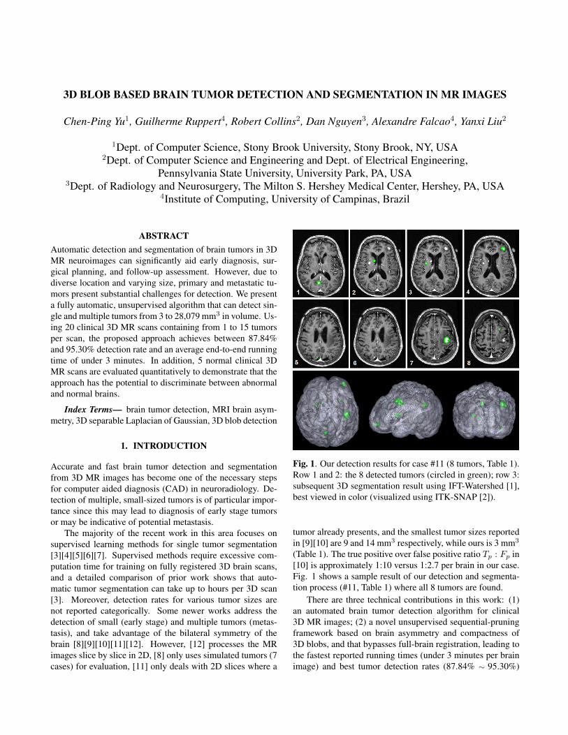
Case Information Tumor Volume (mm3) Results at Three Threshold Levels of C (Tp / Total | Fp)Case# Type # Tumors Mean Min Max γ4 = 0.25 γ5 = 0.20 γ6 = 0.15

1 M 1 12107 12107 12107 1 / 1 2 1 / 1 2 1 / 1 62 P 1 1448 1448 1448 1 / 1 3 1 / 1 9 1 / 1 163 M 2 10809 3532 18086 1 / 2 2 2 / 2 6 2 / 2 84 M 4 355.25 140 732 4 / 5 2 4 / 5 2 4 / 5 35 M 11 135.91 4 625 9 / 11 6 9 / 11 8 10 / 11 116 P 1 11913 11913 11913 1 / 1 2 1 / 1 5 1 / 1 67 M 15 82.31 3 422 12 / 15 10 14 / 15 15 15 / 15 208 P 1 2262 2262 2262 1 / 1 2 1 / 1 5 1 / 1 89 M 1 3723 3723 3723 1 / 1 6 1 / 1 10 1 / 1 1210 M 5 5879 5 28079 4 / 5 2 5 / 5 7 5 / 5 811 M 8 464.63 18 2226 8 / 8 6 8 / 8 6 8 / 8 812 P 1 12639 12639 12639 1 / 1 4 1 / 1 5 1 / 1 1013 M 1 22033 22033 22033 1 / 1 2 1 / 1 6 1 / 1 1114 M 1 150 150 150 1 / 1 9 1 / 1 15 1 / 1 1815 M 2 10829 3617 18041 2 / 2 3 2 / 2 8 2 / 2 1416 M 8 602.25 25 2145 4 / 8 1 6 / 8 5 6 / 8 617 M 5 192.40 12 533 5 / 5 3 5 / 5 6 5 / 5 1218 M 10 572.90 9 3553 6 / 10 3 6 / 10 5 6 / 10 919 M 2 179.50 56 303 2 / 2 0 2 / 2 0 2 / 2 320 M 4 487.50 30 1426 3 / 4 6 4 / 4 12 4 / 4 20

Total - - - - - 68 / 85 74 75 / 85 137 77 / 85 209Recall - - - - - 87.84±17.47% 94.51±11.23% 95.30±10.92%

Precision - - - - - 46.17±23.44% 35.71±24.18% 26.03±17.78%Tp : Fp - - - - - 1 : 1.09 1 : 1.83 1 : 2.71

Final Blob # - - - - - 7.10±5.05 10.60±6.02 14.30±6.99

Table 1. Automatic brain tumor detection results are shown at three threshold levels for C with the highest recall rates (γ4,5,6,Fig. 4B). Case-Type P and M stand for Primary and Metastatic tumors respectively. The smallest volume of the detectedtumor is 3 mm3 (case 5), and the largest is 28,079 mm3 (case 10).

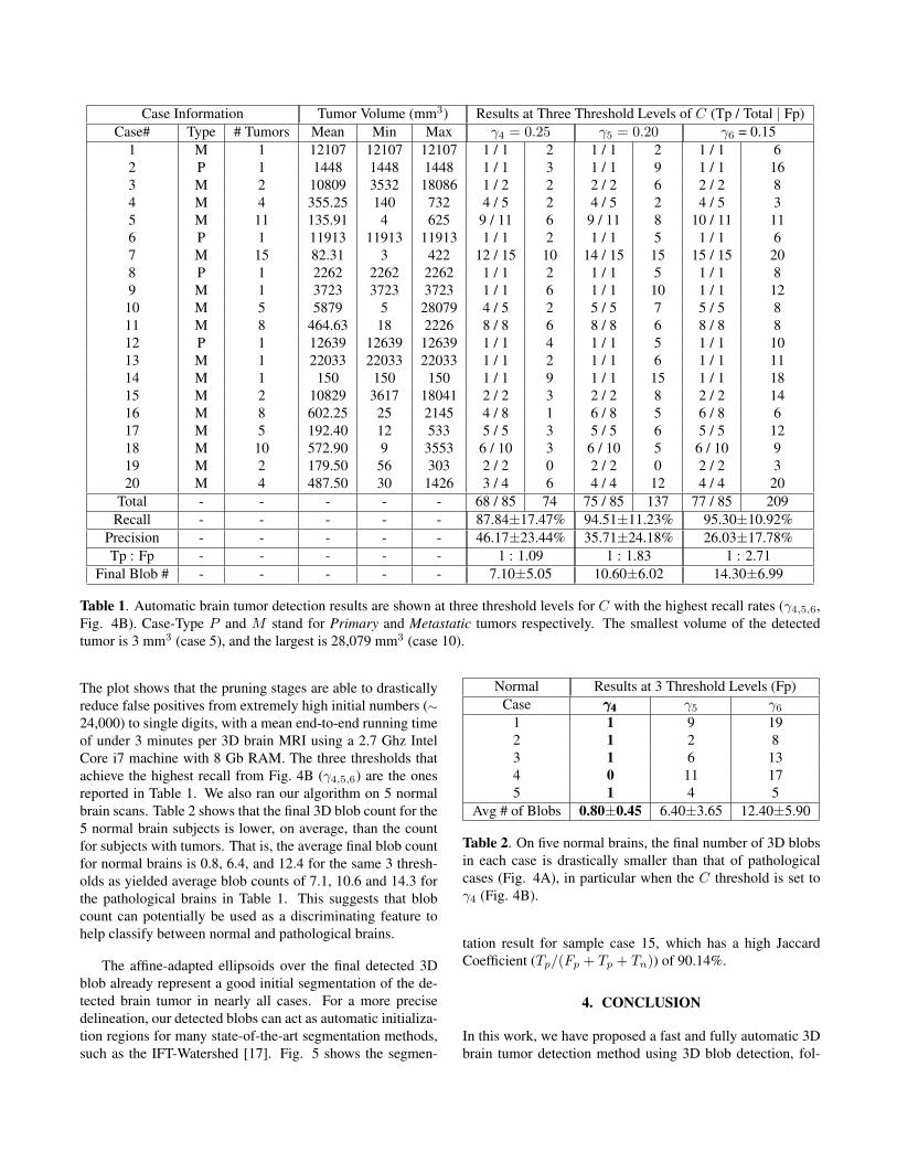
The plot shows that the pruning stages are able to drasticallyreduce false positives from extremely high initial numbers (∼24,000) to single digits, with a mean end-to-end running timeof under 3 minutes per 3D brain MRI using a 2.7 Ghz IntelCore i7 machine with 8 Gb RAM. The three thresholds thatachieve the highest recall from Fig. 4B (γ4,5,6) are the onesreported in Table 1. We also ran our algorithm on 5 normalbrain scans. Table 2 shows that the final 3D blob count for the5 normal brain subjects is lower, on average, than the countfor subjects with tumors. That is, the average final blob countfor normal brains is 0.8, 6.4, and 12.4 for the same 3 thresh-olds as yielded average blob counts of 7.1, 10.6 and 14.3 forthe pathological brains in Table 1. This suggests that blobcount can potentially be used as a discriminating feature tohelp classify between normal and pathological brains.

The affine-adapted ellipsoids over the final detected 3Dblob already represent a good initial segmentation of the de-tected brain tumor in nearly all cases. For a more precisedelineation, our detected blobs can act as automatic initializa-tion regions for many state-of-the-art segmentation methods,such as the IFT-Watershed [17]. Fig. 5 shows the segmen-

Normal Results at 3 Threshold Levels (Fp)Case γ4γ4γ4 γ5 γ6

1 1 9 192 1 2 83 1 6 134 0 11 175 1 4 5

Avg # of Blobs 0.80±0.45 6.40±3.65 12.40±5.90

Table 2. On five normal brains, the final number of 3D blobsin each case is drastically smaller than that of pathologicalcases (Fig. 4A), in particular when the C threshold is set toγ4 (Fig. 4B).

tation result for sample case 15, which has a high JaccardCoefficient (Tp/(Fp + Tp + Tn)) of 90.14%.

4. CONCLUSION

In this work, we have proposed a fast and fully automatic 3Dbrain tumor detection method using 3D blob detection, fol-

Fig. 5. A: case #15 original image, showing 2 tumors in arepresentative slice; B: the detection result of our proposedmethod; C: the binary mask from the detected 3D blobs forautomatic segmentation seeding; D: the 3D segmentation re-sult, which has a Jaccard Coefficient of 90.14%. See our sup-plemental movie for additional examples.

lowed by principles of shape compactness and asymmetry.Our use of the Laplacian of Gaussian to find 3D blobs is scale-invariant and highly sensitive to small abnormalities (as smallas 3 mm3). Subsequent affine adaptation and asymmetry-based pruning stages result in low false positive Fp tumor de-tections. Our average 95.3% detection rate, average 3-10 falsepositives Fp per brain (Table 1), and under 3 minute run-time(on a standard PC running Intel Core i7) are an improvementover state-of-the-art algorithms (average detection rate 90%,average Fp per brain 34.8 by [9][10], and 30 minutes usingtemplate matching in [10]). The detection results can also beapplied to other brain abnormality detection tasks using the fi-nal 3D blobs as features. Finally, our detection results can beused as foreground seeds for automatic tumor delineation us-ing any state-of-the-art segmentation method, and the numberand salience of tumor hypotheses found may serve as poten-tial discriminative measures between normal and pathologicalbrains.

5. ACKNOWLEDGEMENT

This work is supported in part by a Grace Woodward grantfor collaborative research in engineering and medicine at PSU(PI: Liu/Nguyen) and by the CNPq agency. We are gratefulto Dr. R. Kikinis’s lab for providing some of the brain scans.

6. REFERENCES

[1] R. Audigier and R. A. Lotufo, “Watershed by image forest-ing transform, tie-zone, and theoretical relationships with other

watershed definitions,” in International Symposium on Mathe-matical Morphology, 2007.

[2] P.A. Yushkevich, J. Piven, H.C. Hazlett, R.G. Smith, S. Ho,J.C. Gee, and G. Gerig, “User-guided 3D active contour seg-mentation of anatomical structures: Significantly improved ef-ficiency and reliability,” Neuroimage, 2006.

[3] J.J. Corso, E. Sharon, S. Dube, S. El-Saden, U. Sinha, andA. Yuille, “Efficient multilevel brain tumor segmentation withintegrated bayesian model classification,” TMI, 2008.

[4] D. Cobzas, N. Birkbeck, M. Schmidt, M. Jagersand, andA. Murtha, “3D variational brain tumor segmentation usinga high dimensional feature set,” in ICCV, 2007.

[5] C.H. Lee, S. Wang, A. Murtha, M.R.G. Brown, and R. Greiner,“Segmenting brain tumors using pseudo-conditional randomfields,” in MICCAI, 2008.

[6] C. Lee, R. Greiner, and M. Schmidt, “Support vector randomfields for spatial classification,” in PKDD, 2005.

[7] D. Koshy, C. Yu, D. T.D. Nguyen, S. Kashyap, R. T. Collins,and Y. Liu, “Supervised machine learning for brain tumordetection in structural MRI,” Radiological Society of NorthAmerica (RSNA), 2011.

[8] Sahar Ghanavati, Junning Li, Ting Liu, Paul S Babyn, WendyDoda, and G Lampropoulos, “Automatic brain tumor detectionin magnetic resonance images,” in ISBI, 2012.

[9] T. Sugimoto, S. Katsuragawa, T. Hirai, R. Murakami, andY. Yamashita, “Computerized detection of metastatic brain tu-mors on contrast-enhanced 3D MR images by using a selectiveenhancement filter,” in World Congress on Medical Physicsand Biomedical Engineering, 2010.

[10] R. Ambrosini and P. Wang, “Computer-aided detection ofmetastatic brain tumors using automated three-dimensionaltemplate matching,” Journal of MRI, 2010.

[11] N. Ray, B. N. Saha, and M. Brown, “Locating brain tumorsfrom MR imagery using symmetry,” in Asilomar SSC, 2007.

[12] C. Yu, G. C.S. Ruppert, D. TD Nguyen, A. X. Falcao, andY. Liu, “Statistical asymmetry-based brain tumor segmentationfrom 3D MR images.,” in BIOSIGNALS, 2012.

[13] G. C. S. Ruppert, L. Teverovskiy, C. Yu, A. X. Falcao, andY. Liu, “A new symmetry-based method for mid-sagittal planeextraction in neuroimages,” in ISBI, 2011.

[14] S.M. Smith, “Fast robust automated brain extraction,” HumanBrain Mapping, 2002.

[15] Y. Liu, R. T. Collins, and W. E. Rothfus, Automatic extractionof the central symmetry (mid-sagittal) plane from neuroradiol-ogy images, Carnegie Mellon University, the Robotics InstituteTR-96-40, 1996.

[16] E. Levina and P. Bickel, “The earth mover’s distance is themallows distance: Some insights from statistics,” in ICCV,2001.

[17] R. Lotufo and A. Falcao, “The ordered queue and the optimal-ity of the watershed approaches,” in Mathematical Morphologyand its Applications to Image and Signal Processing, 2002.